Embed Size (px)
Citation preview
Database Management Systems 3ed, R. Ramakrishnan and J. Gehrke 1
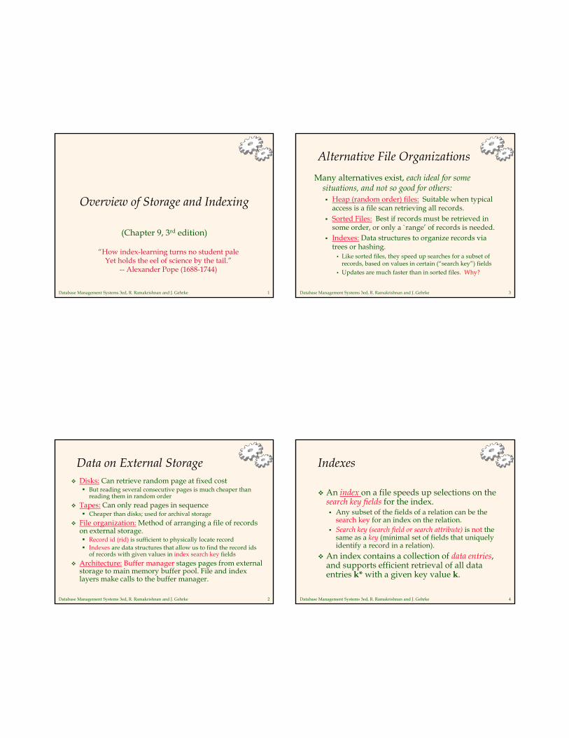
Overview of Storage and Indexing
(Chapter 9, 3rd edition)
“How index-learning turns no student paleYet holds the eel of science by the tail.”
-- Alexander Pope (1688-1744)
Database Management Systems 3ed, R. Ramakrishnan and J. Gehrke 2
Data on External Storage Disks: Can retrieve random page at fixed cost
But reading several consecutive pages is much cheaper than reading them in random order
Tapes: Can only read pages in sequence Cheaper than disks; used for archival storage
File organization: Method of arranging a file of records on external storage. Record id (rid) is sufficient to physically locate record Indexes are data structures that allow us to find the record ids
of records with given values in index search key fields
Architecture: Buffer manager stages pages from external storage to main memory buffer pool. File and index layers make calls to the buffer manager.
Database Management Systems 3ed, R. Ramakrishnan and J. Gehrke 3
Alternative File Organizations
Many alternatives exist, each ideal for some situations, and not so good for others: Heap (random order) files: Suitable when typical
access is a file scan retrieving all records. Sorted Files: Best if records must be retrieved in
some order, or only a `range’ of records is needed. Indexes: Data structures to organize records via
trees or hashing. • Like sorted files, they speed up searches for a subset of
records, based on values in certain (“search key”) fields• Updates are much faster than in sorted files. Why?
Database Management Systems 3ed, R. Ramakrishnan and J. Gehrke 4
Indexes
An index on a file speeds up selections on the search key fields for the index. Any subset of the fields of a relation can be the
search key for an index on the relation. Search key (search field or search attribute) is not the
same as a key (minimal set of fields that uniquely identify a record in a relation).
An index contains a collection of data entries, and supports efficient retrieval of all data entries k* with a given key value k.

Database Management Systems 3ed, R. Ramakrishnan and J. Gehrke 5
Alternatives for Data Entry k* in Index
Three alternatives: Data record with key value k <k, rid of data record with search key value k> <k, list of rids of data records with search key k>
Choice of alternative for data entries is orthogonal to the indexing technique used to locate data entries with a given key value k. Examples of indexing techniques: B+ trees, hash-
based structures Typically, index contains auxiliary information that
directs searches to the desired data entries
Database Management Systems 3ed, R. Ramakrishnan and J. Gehrke 6
Alternatives for Data Entries (Contd.) Alternative 1:
If this is used, index structure is a file organization for data records (instead of a Heap file or sorted file).
At most one index on a given collection of data records can use Alternative 1. (Otherwise, data records are duplicated, leading to redundant storage and potential inconsistency.)
If data records are very large, # of pages containing data entries is high. Implies size of auxiliary information in the index is also large, typically.
Database Management Systems 3ed, R. Ramakrishnan and J. Gehrke 7
Alternatives for Data Entries (Contd.)
Alternatives 2 and 3: Data entries typically much smaller than data
records. So, better than Alternative 1 with large data records, especially if search keys are small. (Portion of index structure used to direct search, which depends on size of data entries, is much smaller than with Alternative 1.)
Alternative 3 more compact than Alternative 2, but leads to variable sized data entries even if search keys are of fixed length.
Database Management Systems 3ed, R. Ramakrishnan and J. Gehrke 8
Index Classification
Primary vs. secondary: If search key contains primary key, then called primary index. Unique index: Search key contains a candidate key.
Clustered vs. unclustered: If order of data records is the same as, or `close to’, order of data entries, then called clustered index. Alternative 1 implies clustered; in practice, clustered also
implies Alternative 1 (since sorted files are rare). A file can be clustered (or sorted) on at most one search key. Cost of retrieving data records through index varies greatly
based on whether index is clustered or not! If there are multiple indexes, only one can be clustered! Need to
be chosen judiciously.

Database Management Systems 3ed, R. Ramakrishnan and J. Gehrke 9
Clustered vs. Unclustered Index Suppose that Alternative (2) is used for data entries,
and that the data records are stored in a Heap file. To build clustered index, first sort the Heap file (with
some free space on each page for future inserts). Overflow pages may be needed for inserts. (Thus, order of
data recs is `close to’, but not identical to, the sort order.)
Index entries
Data entries
direct search for
(Index File)
(Data file)
Data Records
data entries
Data entries
Data Records
CLUSTERED UNCLUSTERED
Database Management Systems 3ed, R. Ramakrishnan and J. Gehrke 10
Index Classification (Contd.) Dense vs. Sparse: Dense: an index record
appears for every search key in the file!
Sparse: index records are created only for some of the records Alternative 1 always leads
to dense index. Why? Every sparse index is
clustered! Why? Sparse indexes are smaller.
why? However, some useful
optimizations are based on dense indexes (e.g., count)
Ashby, 25, 3000
Smith, 44, 3000
Ashby
Cass
Smith
22
25
30
40
44
44
50
Sparse Indexon
Name Data File
Dense Indexon
Age
33
Bristow, 30, 2007
Basu, 33, 4003
Cass, 50, 5004
Tracy, 44, 5004
Daniels, 22, 6003
Jones, 40, 6003
Database Management Systems 3ed, R. Ramakrishnan and J. Gehrke 11
Hash-Based Indexes
Good for equality selections. Why?• Index is a collection of buckets. Bucket = primary
page plus zero or more overflow pages.• Hashing function h: h(r) = bucket in which
record r belongs. h looks at the search key fields of r.
If Alternative (1) is used, the buckets contain the data records; otherwise, they contain <key, rid> or <key, rid-list> pairs.
Database Management Systems 3ed, R. Ramakrishnan and J. Gehrke 12
B+ Tree Indexes (B stands for ?)
Leaf pages contain data (search key) entries, and are chained (prev & next). Non-leaf pages contain index entriesand direct searches:Data pages are separate from Leaf index pages (not shown)!!
P0 K 1 P 1 K 2 P 2 K m P m
index entry
Non-leaf
Pages
Pages
Leaf
Database Management Systems 3ed, R. Ramakrishnan and J. Gehrke 13
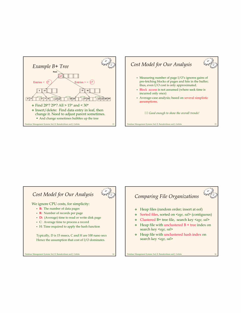
Example B+ Tree
Find 28*? 29*? All > 15* and < 30* Insert/delete: Find data entry in leaf, then
change it. Need to adjust parent sometimes. And change sometimes bubbles up the tree
2* 3*
Root
17
30
14* 16* 33* 34* 38* 39*
135
7*5* 8* 22* 24*
27
27* 29*
Entries < 17 Entries > = 17
Database Management Systems 3ed, R. Ramakrishnan and J. Gehrke 14
Cost Model for Our Analysis
We ignore CPU costs, for simplicity: B: The number of data pages R: Number of records per page D: (Average) time to read or write disk page C: Average time to process a record H: Time required to apply the hash function
Typically, D is 15 msecs, C and H are 100 nano secsHence the assumption that cost of I/O dominates.
Database Management Systems 3ed, R. Ramakrishnan and J. Gehrke 15
Cost Model for Our Analysis
Measuring number of page I/O’s ignores gains of pre-fetching blocks of pages and hits in the buffer; thus, even I/O cost is only approximated.
Block access is not assumed (where seek time is incurred only once)
Average-case analysis; based on several simplistic assumptions.
Good enough to show the overall trends!
Database Management Systems 3ed, R. Ramakrishnan and J. Gehrke 16
Comparing File Organizations
Heap files (random order; insert at eof) Sorted files, sorted on <age, sal> (contiguous) Clustered B+ tree file, search key <age, sal> Heap file with unclustered B + tree index on
search key <age, sal> Heap file with unclustered hash index on
search key <age, sal>
Database Management Systems 3ed, R. Ramakrishnan and J. Gehrke 17
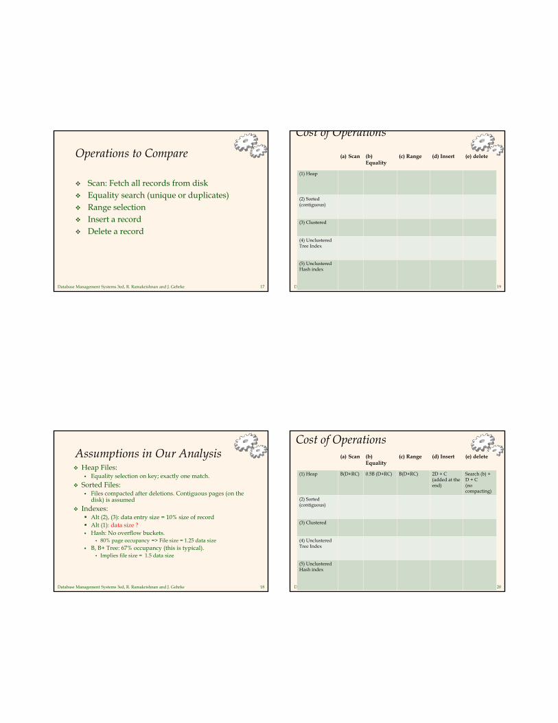
Operations to Compare
Scan: Fetch all records from disk Equality search (unique or duplicates) Range selection Insert a record Delete a record
Database Management Systems 3ed, R. Ramakrishnan and J. Gehrke 18
Assumptions in Our Analysis Heap Files:
Equality selection on key; exactly one match.
Sorted Files: Files compacted after deletions. Contiguous pages (on the
disk) is assumed
Indexes: Alt (2), (3): data entry size = 10% size of record Alt (1): data size ? Hash: No overflow buckets.
• 80% page occupancy => File size = 1.25 data size B, B+ Tree: 67% occupancy (this is typical).
• Implies file size = 1.5 data size
Database Management Systems 3ed, R. Ramakrishnan and J. Gehrke 19
Cost of Operations
Several assumptions underlie these (rough) estimates!
(a) Scan (b) Equality
(c) Range (d) Insert (e) delete
(1) Heap
(2) Sorted(contiguous)
(3) Clustered
(4) UnclusteredTree Index
(5) UnclusteredHash index
Database Management Systems 3ed, R. Ramakrishnan and J. Gehrke 20
Cost of Operations
Several assumptions underlie these (rough) estimates!
(a) Scan (b) Equality
(c) Range (d) Insert (e) delete
(1) Heap B(D+RC) 0.5B (D+RC) B(D+RC) 2D + C (added at the end)
Search (b) + D + C(no compacting)
(2) Sorted(contiguous)
(3) Clustered
(4) UnclusteredTree Index
(5) UnclusteredHash index

Database Management Systems 3ed, R. Ramakrishnan and J. Gehrke 21
Cost of Operations
Several assumptions underlie these (rough) estimates!
(a) Scan (b) Equality
(c) Range (d) Insert (e) delete
(1) Heap B(D+RC)
Cannot do better!
0.5B (D+RC)
Not good
B(D+RC)
Not good
2D + C (at the end)
Good
Search (b) + C+ D
Not good
(2) Sorted(contiguous)
(3) Clustered
(4) UnclusteredTree Index
(5) UnclusteredHash index
Database Management Systems 3ed, R. Ramakrishnan and J. Gehrke 22
Cost of Operations
Several assumptions underlie these (rough) estimates!
(a) Scan (b) Equality
(c) Range (d) Insert (e) delete
(1) Heap B(D+RC)
Cannot do better!
0.5B (D+RC)
Not good
B(D+RC)
Not good
2D + C (at the end)
Good
Search (b) + C+ D
Not good
(2) Sorted(contiguous)
B(D+RC) Dlog 2 B + 2 comparisons for each page + Clog2 R
Dlog 2 B + + matching pages(mp)*D + mp*RC
Search(b) + 2*0.5B (D+RC) (need to move records)
Search(b) + 2*0.5B (D+RC) (needs moving records)
(3) Clustered
(4) UnclusteredTree Index
(5) UnclusteredHash index
Database Management Systems 3ed, R. Ramakrishnan and J. Gehrke 23
Cost of Operations
Several assumptions underlie these (rough) estimates!
(a) Scan (b) Equality
(c) Range (d) Insert (e) delete
(1) Heap B(D+RC)Cannot do better
0.5B (D+RC)Not good
B(D+RC)
Not good
2D + C (at the end)Good
Search (b) + C+ DNot good
(2) Sorted(contiguous)
B(D+RC)Cannot do better
Dlog 2 B +
Clog2 R Good
Dlog 2 B + + matching pages*D + mp*RCGood
Search(b) + 2*0.5B (D+RC) Not good
Search(b) + 2*0.5B (D+RC) Not good
(3) Clustered B+ tree
(4) UnclusteredB+ Tree Index (Alt 2)
(5) UnclusteredHash index
Database Management Systems 3ed, R. Ramakrishnan and J. Gehrke 24
Cost of Operations
Several assumptions underlie these (rough) estimates!
(a) Scan (b) Equality
(c) Range (d) Insert (e) delete
(1) Heap B(D+RC)Cannot do better
0.5B (D+RC)Not good
B(D+RC)
Not good
2D + C (at the end)Good
Search (b) + C+ DNot good
(2) Sorted(contiguous)
B(D+RC)Cannot do better
Dlog 2 B +
Clog2 R Good
Dlog 2 B + + matching pages*D + mp*RCGood
Search(b) + 2*0.5B (D+RC) Not good
Search(b) + 2*0.5B (D+RC) Not good
(3) Clustered B+ tree
1.5B(D+RC)
DlogF 1.5B + Clog2 R
Dlog F 1.5B + + mp*D + mp*RC
Search + D + Clog2 R (assumes free space)
Search + D + Clog2 R
(4) UnclusteredB+ Tree Index (Alt 2)
(5) UnclusteredHash index
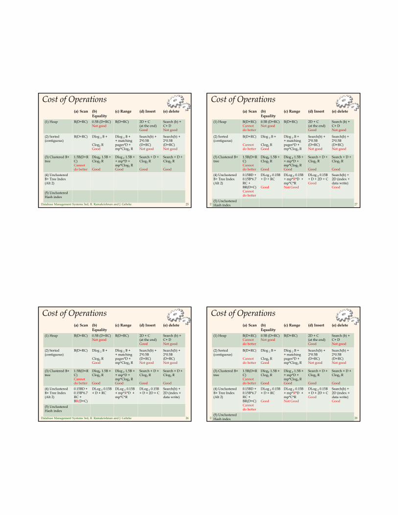
Database Management Systems 3ed, R. Ramakrishnan and J. Gehrke 25
Cost of Operations
Several assumptions underlie these (rough) estimates!
(a) Scan (b) Equality
(c) Range (d) Insert (e) delete
(1) Heap B(D+RC) 0.5B (D+RC)Not good
B(D+RC) 2D + C (at the end)Good
Search (b) + C+ DNot good
(2) Sorted(contiguous)
B(D+RC) Dlog 2 B +
Clog2 R Good
Dlog 2 B + + matching pages*D + mp*Clog2 R
Search(b) + 2*0.5B (D+RC) Not good
Search(b) + 2*0.5B (D+RC) Not good
(3) Clustered B+ tree
1.5B(D+RC)Cannot do better
DlogF 1.5B + Clog2 R
Good
Dlog F 1.5B + + mp*D + mp*Clog2 R Good
Search + D + Clog2 R
Good
Search + D + Clog2 R
Good
(4) UnclusteredB+ Tree Index (Alt 2)
(5) UnclusteredHash index
Database Management Systems 3ed, R. Ramakrishnan and J. Gehrke 26
Cost of Operations
Several assumptions underlie these (rough) estimates!
(a) Scan (b) Equality
(c) Range (d) Insert (e) delete
(1) Heap B(D+RC) 0.5B (D+RC)Not good
B(D+RC) 2D + C (at the end)Good
Search (b) + C+ DNot good
(2) Sorted(contiguous)
B(D+RC) Dlog 2 B +
Clog2 R Good
Dlog 2 B + + matching pages*D + mp*Clog2 R
Search(b) + 2*0.5B (D+RC) Not good
Search(b) + 2*0.5B (D+RC) Not good
(3) Clustered B+ tree
1.5B(D+RC)Cannot do better
DlogF 1.5B + Clog2 R
Good
Dlog F 1.5B + + mp*D + mp*Clog2 R Good
Search + D + Clog2 R
Good
Search + D + Clog2 R
Good
(4) UnclusteredB+ Tree Index (Alt 2)
0.15BD + 0.15B*6.7RC + BR(D+C)
DLog F 0.15B + D + RC
DLog F 0.15B + mp*R*D + mp*C*R
DLog F 0.15B + D + 2D + C
Search(b) + 2D (index + data write)
(5) UnclusteredHash index
Database Management Systems 3ed, R. Ramakrishnan and J. Gehrke 27
Cost of Operations
Several assumptions underlie these (rough) estimates!
(a) Scan (b) Equality
(c) Range (d) Insert (e) delete
(1) Heap B(D+RC)Cannot do better
0.5B (D+RC)Not good
B(D+RC) 2D + C (at the end)Good
Search (b) + C+ DNot good
(2) Sorted(contiguous)
B(D+RC)
Cannot do better
Dlog 2 B +
Clog2 R Good
Dlog 2 B + + matching pages*D + mp*Clog2 R
Search(b) + 2*0.5B (D+RC) Not good
Search(b) + 2*0.5B (D+RC) Not good
(3) Clustered B+ tree
1.5B(D+RC)Cannot do better
DlogF 1.5B + Clog2 R
Good
Dlog F 1.5B + + mp*D + mp*Clog2 R Good
Search + D + Clog2 R
Good
Search + D + Clog2 R
Good
(4) UnclusteredB+ Tree Index (Alt 2)
0.15BD + 0.15B*6.7RC + BR(D+C)Cannot do better
DLog F 0.15B + D + RC
Good
DLog F 0.15B + mp*R*D + mp*C*RNot Good
DLog F 0.15B + D + 2D + CGood
Search(b) + 2D (index + data write)Good
(5) UnclusteredHash index
Database Management Systems 3ed, R. Ramakrishnan and J. Gehrke 28
Cost of Operations
Several assumptions underlie these (rough) estimates!
(a) Scan (b) Equality
(c) Range (d) Insert (e) delete
(1) Heap B(D+RC)Cannot do better
0.5B (D+RC)Not good
B(D+RC) 2D + C (at the end)Good
Search (b) + C+ DNot good
(2) Sorted(contiguous)
B(D+RC)
Cannot do better
Dlog 2 B +
Clog2 R Good
Dlog 2 B + + matching pages*D + mp*Clog2 R
Search(b) + 2*0.5B (D+RC) Not good
Search(b) + 2*0.5B (D+RC) Not good
(3) Clustered B+ tree
1.5B(D+RC)Cannot do better
DlogF 1.5B + Clog2 R
Good
Dlog F 1.5B + + mp*D + mp*Clog2 R Good
Search + D + Clog2 R
Good
Search + D + Clog2 R
Good
(4) UnclusteredB+ Tree Index (Alt 2)
0.15BD + 0.15B*6.7RC + BR(D+C)Cannot do better
DLog F 0.15B + D + RC
Good
DLog F 0.15B + mp*R*D + mp*C*RNot Good
DLog F 0.15B + D + 2D + CGood
Search(b) + 2D (index + data write)Good
(5) UnclusteredHash index
Database Management Systems 3ed, R. Ramakrishnan and J. Gehrke 29
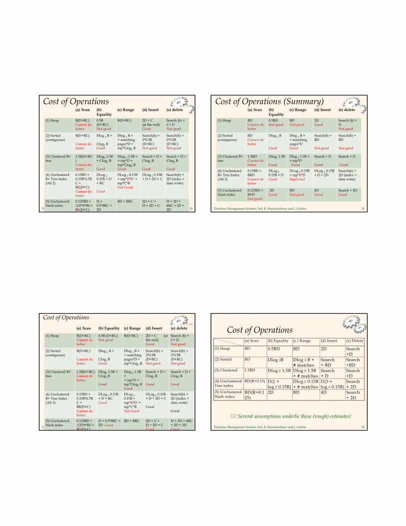
Cost of Operations
Several assumptions underlie these (rough) estimates!
(a) Scan (b) Equality
(c) Range (d) Insert (e) delete
(1) Heap B(D+RC)Cannot do better
0.5B (D+RC)Not good
B(D+RC) 2D + C (at the end)Good
Search (b) + C+ DNot good
(2) Sorted(contiguous)
B(D+RC)
Cannot do better
Dlog 2 B +
Clog2 R Good
Dlog 2 B + + matching pages*D + mp*Clog2 R
Search(b) + 2*0.5B (D+RC) Not good
Search(b) + 2*0.5B (D+RC) Not good
(3) Clustered B+ tree
1.5B(D+RC)Cannot do better
DlogF 1.5B + Clog2 R
Good
Dlog F 1.5B + + mp*D + mp*Clog2 R Good
Search + D + Clog2 R
Good
Search + D + Clog2 R
Good
(4) UnclusteredB+ Tree Index (Alt 2)
0.15BD + 0.15B*6.7RC + BR(D+C)Cannot do better
DLog F0.15B + D + RC
Good
DLog F 0.15B + mp*R*D + mp*C*RNot Good
DLog F 0.15B + D + 2D + C
Search(b) + 2D (index + data write)
(5) UnclusteredHash index
0.125BD + .125*8*RC+BR(D+C)
H + 0.5*8RC +2D
BD + BRC 2D + C +H + 2D + C
H + 2D + 4RC + 2D + 2D
Database Management Systems 3ed, R. Ramakrishnan and J. Gehrke 30
Cost of Operations
Several assumptions underlie these (rough) estimates!
(a) Scan (b) Equality (c) Range (d) Insert (e) delete
(1) Heap B(D+RC)Cannot do better
0.5B (D+RC)Not good
B(D+RC) 2D + C (at the end)Good
Search (b) + C+ DNot good
(2) Sorted(contiguous)
B(D+RC)
Cannot do better
Dlog 2 B +
Clog2 R Good
Dlog 2 B + + matching pages*D + mp*Clog2 R
Search(b) + 2*0.5B (D+RC) Not good
Search(b) + 2*0.5B (D+RC) Not good
(3) Clustered B+ tree
1.5B(D+RC)Cannot do better
DlogF 1.5B + Clog2 R
Good
Dlog F 1.5B + + mp*D + mp*Clog2 R Good
Search + D + Clog2 R
Good
Search + D + Clog2 R
Good
(4) UnclusteredB+ Tree Index (Alt 2)
0.15BD + 0.15B*6.7RC + BR(D+C)Cannot do better
DLog F 0.15B + D + RCGood
DLog F0.15B + mp*R*D + mp*C*RNot Good
DLog F 0.15B + D + 2D + C
Good
Search(b) + 2D (index + data write)
Good
(5) UnclusteredHash index
0.125BD + .125*8*RC+BR(D+C)
H + 0.5*8RC +2D Good
BD + BRC 2D + C +H + 2D + C Good
H + 2D + 4RC + 2D + 2D Good
Database Management Systems 3ed, R. Ramakrishnan and J. Gehrke 31
Cost of Operations (Summary)
Several assumptions underlie these (rough) estimates!
(a) Scan (b) Equality
(c) Range (d) Insert (e) delete
(1) Heap BDCannot do better
0.5BDNot good
BDNot good
2D Good
Search (b) + DNot good
(2) Sorted(contiguous)
BDCannot do better
Dlog 2 B
Good
Dlog 2 B + + matching pages*D Good
Search(b) + BD
Not good
Search(b) + BD
Not good
(3) Clustered B+ tree
1.5BDCannot do better
DlogF 1.5B
Good
Dlog F 1.5B + + mp*D
Good
Search + D
Good
Search + D
Good
(4) UnclusteredB+ Tree Index (Alt 2)
0.15BD + BRDCannot do better
DLog F0.15B + D Good
DLog F 0.15B + mp*R*D Not Good
DLog F 0.15B + D + 2D
Search(b) + 2D (index + data write)
(5) UnclusteredHash index
0.125BD + BRDNot good
2D Good
BDNot good
4DGood
Search + 4D Good
Database Management Systems 3ed, R. Ramakrishnan and J. Gehrke 32
Cost of Operations (a) Scan (b) Equality (c ) Range (d) Insert (e) Delete
(1) Heap BD 0.5BD BD 2D Search +D
(2) Sorted BD Dlog 2B Dlog 2 B + # matches
Search + BD
Search +BD
(3) Clustered 1.5BD Dlog F 1.5B Dlog F 1.5B + # matches
Search + D
Search +D
(4) Unclustered Tree index
BD(R+0.15) D(1 + log F 0.15B)
Dlog F 0.15B + # matches
D(3 + log F 0.15B)
Search + 2D
(5) Unclustered Hash index
BD(R+0.125)
2D BD 4D Search + 2D
Several assumptions underlie these (rough) estimates!
Database Management Systems 3ed, R. Ramakrishnan and J. Gehrke 33
Understanding the Workload
For each query in the workload: Which relations does it access? Which attributes are retrieved? Which attributes are involved in selection/join conditions?
How selective are these conditions likely to be?
For each update in the workload: Which attributes are involved in selection/join conditions?
How selective are these conditions likely to be? The type of update (INSERT/DELETE/UPDATE), and the
attributes that are affected.
Database Management Systems 3ed, R. Ramakrishnan and J. Gehrke 34
Choice of Indexes
What indexes should we create? Which relations should have indexes? What field(s)
should be the search key? Should we build several indexes?
For each index, what kind of an index should it be? Clustered? Hash/tree?
Database Management Systems 3ed, R. Ramakrishnan and J. Gehrke 35
Choice of Indexes (Contd.)
One approach: Consider the most important queries in turn. Consider the best plan using the current indexes, and see if a better plan is possible with an additional index. If so, create it. Obviously, this implies that we must understand how a
DBMS evaluates queries and creates query evaluation plans! For now, we discuss simple 1-table queries.
Before creating an index, must also consider the impact of updates in the workload! Trade-off: Indexes can make queries go faster, updates
slower. Require disk space, too.
Database Management Systems 3ed, R. Ramakrishnan and J. Gehrke 36
Index Selection Guidelines Attributes in WHERE clause are candidates for index keys.
Exact match condition suggests hash index. Range query suggests tree index.
• Clustering is especially useful for range queries; can also help on equality queries if there are many duplicates.
Multi-attribute search keys should be considered when a WHERE clause contains several conditions. Order of attributes is important for range queries. Such indexes can sometimes enable index-only strategies for
important queries.• For index-only strategies, clustering is not important!
Try to choose indexes that benefit as many queries as possible. Since only one index can be clustered per relation, choose it wisely based on important queries that would benefit the most from clustering.

Database Management Systems 3ed, R. Ramakrishnan and J. Gehrke 37
Examples of Clustered Indexes
B+ tree index on E.age can be used to get qualifying tuples. How selective is the condition? Is the index clustered?
Consider the GROUP BY query. If many tuples have E.age > 10, using
E.age index and sorting the retrieved tuples may be costly.
Clustered E.dno index may be better!
Equality queries and duplicates: Clustering on E.hobby helps!
SELECT E.dnoFROM Emp EWHERE E.age>40
SELECT E.dno, COUNT (*)FROM Emp EWHERE E.age>10GROUP BY E.dno
SELECT E.dnoFROM Emp EWHERE E.hobby=‘Stamps’
Database Management Systems 3ed, R. Ramakrishnan and J. Gehrke 38
Indexes with Composite Search Keys
Composite Search Keys: Search on a combination of fields. Equality query: Every field
value is equal to a constant value. E.g. wrt <sal,age> index:
• age=20 and sal =75
Range query: Some field value is not a constant. E.g.:
• age =20; or age=20 and sal > 10
Data entries in index sorted by search key to support range queries. Lexicographic order, or Spatial order.
sue 13 75
bob
cal
joe 12
10
20
8011
12
name age sal
<sal, age>
<age, sal> <age>
<sal>
12,20
12,10
11,80
13,75
20,12
10,12
75,13
80,11
11
12
12
13
10
20
75
80
Data recordssorted by name
Data entries in indexsorted by <sal,age>
Data entriessorted by <sal>
Examples of composite keyindexes using lexicographic order.
Database Management Systems 3ed, R. Ramakrishnan and J. Gehrke 39
Composite Search Keys
To retrieve Emp records with age=30 AND sal=4000, an index on <age,sal> would be better than an index on age or an index on sal. Choice of index key orthogonal to clustering etc.
If condition is: 20<age<30 AND 3000<sal<5000: Clustered tree index on <age,sal> or <sal,age> is best.
If condition is: age=30 AND 3000<sal<5000: Clustered <age,sal> index much better than <sal,age>
index!
Composite indexes are larger, updated more often.
Database Management Systems 3ed, R. Ramakrishnan and J. Gehrke 40
Index-Only Plans
A number of queries can be answered without retrieving any tuples from one or more of the relations involved if a suitable index is available.
SELECT D.dnoFROM Dept D, Emp EWHERE D.dno=E.dno
SELECT D.dno, E.eidFROM Dept D, Emp EWHERE D.dno=E.dno
SELECT E.dno, COUNT(*)FROM Emp EGROUP BY E.dno
SELECT E.dno, MIN(E.sal)FROM Emp EGROUP BY E.dno
SELECT AVG(E.sal)FROM Emp EWHERE E.age=25 ANDE.sal BETWEEN 3000 AND 5000
<E.dno>
<E.dno,E.eid>Tree index!
<E.dno>
<E.dno,E.sal>Tree index!
<E. age,E.sal>or
<E.sal, E.age>Tree!

Database Management Systems 3ed, R. Ramakrishnan and J. Gehrke 41
Index-Only Plans (Contd.)
Index-only plans are possible if the key is <dno,age> or we have a tree index with key <age,dno> Which is better? What if we
consider the second query?
SELECT E.dno, COUNT (*)FROM Emp EWHERE E.age=30GROUP BY E.dno
SELECT E.dno, COUNT (*)FROM Emp EWHERE E.age>30GROUP BY E.dno
Database Management Systems 3ed, R. Ramakrishnan and J. Gehrke 42
Summary
Many alternative file organizations exist, each appropriate in some situation.
If selection queries are frequent, sorting the file or building an index is important. Hash-based indexes only good for equality search. Sorted files and tree-based indexes best for range
search; also good for equality search. (Files rarely kept sorted in practice; B+ tree index is better.)
Index is a collection of data entries plus a way to quickly find entries with given key values.
Database Management Systems 3ed, R. Ramakrishnan and J. Gehrke 43
Summary (Contd.)
Data entries can be actual data records, <key, rid> pairs, or <key, rid-list> pairs. Choice orthogonal to indexing technique used to
locate data entries with a given key value. Can have several indexes on a given file of
data records, each with a different search key. Indexes can be classified as clustered vs.
unclustered, primary vs. secondary, and dense vs. sparse. Differences have important consequences for utility/performance.
Database Management Systems 3ed, R. Ramakrishnan and J. Gehrke 44
Summary (Contd.) Understanding the nature of the workload for the
application, and the performance goals, is essential to developing a good design. What are the important queries and updates? What
attributes/relations are involved? Indexes must be chosen to speed up important
queries (and perhaps some updates!). Index maintenance overhead on updates to key fields. Choose indexes that can help many queries, if possible. Build indexes to support index-only strategies. Clustering is an important decision; only one index on a
given relation can be clustered! Order of fields in composite index key can be important.