JOHNS HOPKINS APL TECHNICAL DIGEST VOLUME 29 NUMBER 1 (2010) 9shyshyshyshy

Tthe guidance system The types of steering commands vary depending on the phase of flight and the type of interceptor For example in the boost phase the flight control system may be designed to force the missile to track a desired flight-path angle or attitude In the midcourse and terminal phases the system may be designed to track acceleration commands to effect an intercept of the target This article explores several aspects of the missile flight control system including its role in the overall missile system its subsystems types of flight control systems design objectives and design challenges Also discussed are some of APLrsquos contributions to the field which have come primarily through our role as Technical Direction Agent on a variety of Navy missile programs

he flight control system is a key element that allows the missile to meet its system performance requirements The objective of the flight control system

is to force the missile to achieve the steering commands developed by

INTRODUCTIONThe missile flight control system is one element of

the overall homing loop Figure 1 is a simplified block diagram of the missile homing loop configured for the terminal phase of flight when the missile is approaching intercept with the target The missile and target motion relative to inertial space can be combined mathemati-cally to obtain the relative motion between the missile and the target The terminal sensor typically an RF or IR seeker measures the angle between an inertial refer-ence and the missile-to-target line-of-sight (LOS) vector

which is called the LOS angle The state estimator eg a Kalman filter uses LOS angle measurements to estimate LOS angle rate and perhaps other quantities such as target acceleration The state estimates feed a guidance law that develops the flight control commands required to intercept the target The flight control system forces the missile to track the guidance commands resulting in the achieved missile motion The achieved missile motion alters the relative geometry which then is sensed and used to determine the next set of flight control

Overview of Missile Flight Control Systems

Paul B Jackson

P B JACKSON

JOHNS HOPKINS APL TECHNICAL DIGEST VOLUME 29 NUMBER 1 (2010)10

commands and so on This loop continues to operate until the missile intercepts the target

In the parlance of feedback control the homing loop is a feedback control system that regulates the LOS angle rate to zero As such the overall stability and performance of this control system are determined by the dynamics of each element in the loop Conse-quently the flight control system cannot be designed in a vacuum Instead it must be designed in concert with the other elements to meet overall homing-loop perfor-mance requirements in the presence of target maneu-vers and other disturbances in the system eg terminal sensor noise (not shown in Fig 1) which can negatively impact missile performance

The remainder of this article is divided into six sec-tions The first section discusses the specific elements of the flight control system Particular emphasis is placed on understanding the dynamics of the missile and how they affect the flight control system designer The next three sections describe different types of flight control systems objectives to be considered in their design and a brief design example The last two sections discuss some of the challenges that need to be addressed in the future and APLrsquos contributions to Navy systems and the field in general

FLIGHT CONTROL SYSTEM ELEMENTSAs noted above the flight control system is one ele-

ment of the overall homing loop Figure 2 shows the basic elements of the flight control system which itself is another feedback control loop within the overall homing loop depicted in Fig 1 An inertial measurement unit (IMU) measures the missile translational accelera-tion and angular velocity The outputs of the IMU are

combined with the guidance commands in the autopi-lot to compute the commanded control input such as a desired tail-surface deflection or thrust-vector angle An actuator usually an electromechanical system forces the physical control input to follow the commanded control input The airframe dynamics respond to the control input The basic objective of the flight control system is to force the achieved missile dynamics to track the guidance commands in a well-controlled manner The figures of merit (FOMs) used to assess how well the flight control system works are discussed in Flight Control System Design Objectives This section provides an overview of each element of the flight control loop

Guidance InputsThe inputs to the flight control system are outputs

from the guidance law that need to be followed to ulti-mately effect a target intercept The specific form of the flight control system inputs (acceleration commands attitude commands etc) depends on the specific appli-cation (discussed later) In general the flight control system must be designed based on the expected charac-teristics of the commands which are determined by the other elements of the homing loop and overall system requirements Characteristics of concern can be static dynamic or both An example of a static characteris-tic is the maximum input that the flight control system is expected to be able to track For instance a typical rule of thumb for intercepting a target that has constant acceleration perpendicular to the LOS is for the missile to have a 31 acceleration advantage over the target If the missile system is expected to intercept a 10-g accel-erating threat then the flight control system should be able to force the missile to maintain a 30-g acceleration An example of a dynamic characteristic is the expected frequency content of the command For instance rapid changes in the command are expected as the missile approaches intercept against a maneuvering threat but the input commands may change more slowly during

Targetdynamics

Relativegeometry

Stateestimator

Terminalsensor

Guidancelaw

Flight controlsystem

Figure 1 The flight control system is one element in the missile homing loop The inertial missile motion controlled by the flight control system combines with the target motion to form the rela-tive geometry between the missile and target The terminal sensor measures the missile-to-target LOS angle The state estimator forms an estimate of the LOS angle rate which in turn is input to the guidance law The output of the guidance law is the steering command typically a translational acceleration The flight control system uses the missile control effectors such as aerodynamic tail surfaces to force the missile to track steering commands to achieve a target intercept

Guidancelaw Autopilot Actuator

IMU

Airframedynamics

Figure 2 The four basic elements of the flight control system are shown in the gray box The IMU senses the inertial motion of the missile Its outputs and the inputs from the guidance law are com-bined in the autopilot to form a command input to the control effector such as the commanded deflection angle to an aerody-namic control surface The actuator turns the autopilot command into the physical motion of the control effector which in turn influences the airframe dynamics to track the guidance command

MISSILE FLIGHT CONTROL SYSTEMS

JOHNS HOPKINS APL TECHNICAL DIGEST VOLUME 29 NUMBER 1 (2010) 11shyshyshyshy

the midcourse phase of flight where the objective is to keep the missile on an approximate collision path or to minimize energy loss Other dynamic characteristics of concern include the guidance command update rate and the amount of terminal sensor noise flowing into the flight control system and causing unnecessary con-trol actuator activity

Airframe DynamicsRecall that the objective of the flight control system

is to force the missile dynamics to track the input com-mand The dynamics of the airframe are governed by fundamental equations of motion with their specific characteristics determined by the missile aerodynamic response propulsion and mass properties Assuming that missile motion is restricted to the vertical plane (typical for early concept development) the equations of motion that govern the missile dynamics can be devel-oped in straightforward fashion

Consider the diagram in Fig 3 which shows the mis-sile flying in space constrained to the vertical plane The angle between the inertial reference axis and the mis-sile velocity vector is called the flight-path angle g The angle from the velocity vector to the missile centerline is called the angle of attack (AOA) a The angle from the inertial reference to the missile centerline is called the pitch angle Acceleration in the direction normal to the missile Az derives from two sources The non-zero AOA generates aerodynamic lift Normal acceleration

V

Inertial reference

Az

Figure 3 In the pitch plane the missile dynamics and kinemat-ics can be described by four variables Az is the component of the translational acceleration normal to the missile longitudinal axis The AOA a is a measure of how the missile is oriented rela-tive to the airflow and is the angle between the missile velocity vector and the missile longitudinal axis The flight-path angle g is a measure of the direction of travel relative to inertial space ie the angle between the missile velocity vector and an inertial refer-ence The pitch angle defines the missile orientation relative to inertial space and is the angle between the inertial reference and the missile longitudinal axis

also can be developed by a control input d such as tail-fin deflection or thrust-deflection angle In general the missile acceleration also has a component along the centerline due to thrust and drag For the simple model being developed here we assume that this acceleration is negligible

Based on the diagram in Fig 3 the fundamental rela-tionship among the three angles above is

amp amp = ndash rarr = ndash amp (1)

The angular acceleration is the moment applied to the airframe divided by the moment of inertia

ampamp = M( )J

(2)

The applied moment is a function of the control input d and the aerodynamic force induced by the AOA The rate of change of the flight-path angle is the component of missile acceleration perpendicular to the velocity vector divided by the magnitude of the velocity vector Assuming that the AOA is small the flight-path angle rate is

amp = asympA

V

A

Vz zcos( )

(3)

The normal acceleration is determined by the forces applied to the missile divided by its mass

Amz

z= F( )

(4)

The applied force is a function of the control input d and the aerodynamic force induced by the AOA Substi-tuting Eqs 3 and 4 into Eq 1 and combining the result with Eq 2 yields a coupled set of nonlinear differential equations where the state variables are the AOA and the pitch rate

mVzF( )

amp amp = ndash

ampamp = M( )J

(5)

Although these differential equations can be solved numerically an analytical approach often is desirable to fully understand the missile dynamics Therefore the equations of motion are linearized around an operating condition so that linear systems theory can be applied Assuming constant missile speed linearization of Eq 5 yields a second-order state-space description of the mis-sile dynamics

P B JACKSON

JOHNS HOPKINS APL TECHNICAL DIGEST VOLUME 29 NUMBER 1 (2010)12

1 24 3

amp

amp

ampamp

1 24 34

= minus

Z

VM

A

1

0 + minus

=

Z

VM

A Z

B

z

123

0 10

+

C D

Z4

amp

0

amp

(6)

where the numerical coefficients are defined by

Zm

Zm

MJ

=part

=part

=part

1

MJ

=part

partF( )z

1 partF( )z

1 partM( )

1 partM( )

(7)

and are evaluated at the particular operating condition of interest Because these differential equations result from linearization around an operating point the state input and output variables actually represent small signal perturbations around that operating point

These linear differential equations apply for any mis-sile under the stated assumptions However specific dynamics governed by these equations differ depending on the application For example for a tail-controlled endoatmospheric interceptor the dynamics are a weak function of Zd For a thrust-vector-controlled exoatmo-spheric interceptor the aerodynamic forces are negligi-ble and the terms Za and Ma can be set to zero

The linear differential equations determine the dynamic behavior of the missile for small perturbations around the specified operating conditions For example suppose the missile is given an initial condition at an AOA a few degrees away from the nominal AOA around which the dynamics have been linearized One impor-tant question is whether the missile will rotate back to the nominal AOA or diverge in the absence of any corrective control input The answer to this question of stability is determined by the roots of the characteristic polynomial of the state matrix in Eq 6

s M+ + minus =( )sV

2 0 Z

(8)

A necessary and sufficient condition for both roots of this equation to have negative real parts and thus ensure stability is that all of the coefficients be positive Using the conventions in Fig 3 Za is always positive Therefore the stability of the missile in the absence of a control input is determined by the sign of Ma If Ma is

positive the aerodynamic pitching moment forces the missile to diverge from the nominal AOA and the mis-sile is said to be statically unstable If Ma is negative the missile tends to be restored back to the nominal AOA and the missile is said to be statically stable The static stability of the missile is a crucial property that under the stated assumptions is determined solely by the sign of Ma which is in turn determined by the aerodynamic configuration and the location of the missile center of mass

Figure 4 illustrates in the complex s-plane how the roots of the characteristic equation migrate as a function of Ma Again for large positive values of Ma the missile is statically unstable and the dynamics are governed by one unstable real root in the right half of the plane and one stable real root in the left half of the plane As Ma decreases the roots migrate toward the origin When Ma is zero the system has one real stable root in the left half plane and one root at the origin This condition is called neutral stability As Ma becomes more negative the roots migrate toward each other and eventually split apart as a complex pair

The state-space representation in Eq 6 describes the missile dynamics in the time domain A representation in the complex frequency domain can be obtained that relates the input to the system eg tail-deflection angle to the system outputs eg pitch rate and normal accel-eration This type of representation is called the trans-

1086420ndash2ndash4ndash6ndash8ndash10

10

8

6

4

2

0

ndash2

ndash4

ndash6

ndash8

ndash10

M ltlt 0

M ltlt 0

M gtgt 0

M gtgt 0

M = 0

Figure 4 Static stability of the airframe is determined by the slope of the pitching moment curve with respect to the AOA Ma If the slope is positive the missile is statically unstable because one of the roots of the characteristic polynomial of the governing differential equation is in the right half of the complex plane If the slope is negative both roots are in the left half of the plane and the missile is statically stable The case where the slope is zero is called neutral stability with one of the roots at the origin of the complex plane

MISSILE FLIGHT CONTROL SYSTEMS

JOHNS HOPKINS APL TECHNICAL DIGEST VOLUME 29 NUMBER 1 (2010) 13shyshyshyshy

fer function and can be determined from the state-space model using the formula

H s C sI A B D( ) ( ) = minus +minus1 (9)

where s = s + jv is complex fre-quency and A B C and D are defined in Eq 6

In reality missiles are not con-strained to motion in a single plane Figure 5 shows the relevant vari-ables that describe the missile kine-matics in three dimensions The angle of sideslip (AOS) b is the yaw equivalent to the AOA Together they completely specify how the missile body is oriented relative to its velocity vector The three com-ponents of the missile body angular velocity vector resolved in body-fixed coordinates are denoted p q and r denoting the roll pitch and yaw rate respectively The pitch rate q was denoted as in the dis-cussion above where the motion was constrained to the pitch plane

The equations that govern the dynamics of the missile can be developed by applying the NewtonndashEuler equations of motion The

translational motion can be described in terms of the derivatives of the AOA and the AOS The rotational motion can be described in terms of the angu-lar accelerations and takes a simple form assuming that products of inertia are zero

= minus2 2s t

= minus + minusr p

+ minusc tp qamp minusco an se an tanF

mu

F

murzb xb

cos sec tan t

amp 2 2F

mu

F

muyb xb aan tan tan+

q

tan

(10)

amp

amp

amp

pM

IxIz Iy

Ixqr

qM

IyIx Iz

Iypr

rM

I

xb

yb

zb

= minusminus

= minusminus

=zz

Iy IxIz

pqminusminus

(11)

The lateral components of missile inertial translational acceleration resolved in body-fixed coordinates are

A

F

m

AF

m

zzb

yyb

=

=

(12)

In these equations the forces and moments are resolved in body coordinates with components indicated by the subscripts Though not shown explicitly all of the six components of the force and moment vectors are functions of the state variables and three control inputs eg

Figure 5 This diagram defines quantities used to describe the three-dimensional missile kinematics Two angles are used to orient the missile relative to the velocity vector either AOA and AOS or total AOA and aerodynamic roll angle The components of the missile inertial velocity vector resolved in body-fixed axes are u v and w (not shown) The components of the inertial angular velocity vector resolved in body-fixed coordinates are p q and r The missile orientation in inertial space usually is described via three Euler angles typically in yawndashpitchndashroll sequence (not shown)

q

ryB

zBVM

xB

T

A

= AOA = AOST = Total AOAA = Aerodynamic roll angleVM = Missile velocity vector p = Roll angular body rateq = Pitch angular body rater = Yaw angular body ratexB yB zB = Missile body coordinate axes

p

P B JACKSON

JOHNS HOPKINS APL TECHNICAL DIGEST VOLUME 29 NUMBER 1 (2010)14

F f( p q r )zb p y r= (13)

The dynamic equations together are a coupled fifth-order nonlinear differential equation In situations where the mass properties vary with time such as when a rocket motor is burning propellant the differential equation is time-varying as well

Equations 10ndash12 can be linearized around some operat-ing condition of interest by expanding them in a Taylor series and retaining only the first-order terms The result is a linear time-invariant state-space model with three inputs and five outputs

ampx Ax Buy Cx Du

x

u

y A A

T

T

y z

= += +

=

=

=[ pp q r T]

[ p q r]

[ ]p y r

(14)

As in the planar case the state variables control input variables and output variables represent perturbations around the nominal operating condition

Expanding the model to account for yaw and roll in addition to pitch brings a new set of challenges to the flight control designer Foremost among these in many applications is aerodynamic cross-coupling as the total AOA increases in which case aerodynamic surfaces on the leeward side of the missile become shaded by the fuselage resulting in aerodynamic imbalances The net effect typically results in undesirable motion such as roll moment induced by a change in AOA or pitch moment induced by roll control input The flight control system must compensate for these effects An alternative is to simplify the airframe design to minimize cross-coupling but the airframe must be designed with other factors in mind as well such as maximizing the effective range of the missile Compensating for aerodynamic cross- coupling for some missiles is challenging and often limits the maximum total AOA and hence the maxi-mum lateral acceleration that can be achieved by the flight control system

ActuatorThe missile actuator converts the desired control

command developed by the autopilot into physical motion such as rotation of a tail fin that will effect the desired missile motion Actuators for endoatmospheric missiles typically need to be high-bandwidth devices (significantly higher than the desired bandwidth of the flight control loop itself) that can overcome sig-nificant loads Most actuators are electromechanical with hydraulic actuators being an option in certain applications For early design and analysis the actuator

dynamics are modeled with a second-order transfer func-tion (which does not do justice to the actual complexity of the underlying hardware)

s s+ +

(s)

c

a

a a a

=2

2 22

(s) (15)

Although the actuator often is modeled as a linear system for preliminary design and development it is actually a nonlinear device and care must be taken by the flight control designer not to exceed the hardware capabilities Two critical FOMs for the actuator for many endoatmospheric missiles are its rate and position limits The position limit is an effective limit on the moment that the control input can impart on the airframe which in turn limits the maximum AOA and accelera-tion The rate limit essentially limits how fast the actua-tor can cause the missile to rotate which effectively limits how fast the flight control system can respond to changes in the guidance command The performance of a flight control system that commands the actua-tor to exceed its limits can be degraded particularly if the missile is flying at a condition where it is statically unstable

Inertial Measurement UnitThe IMU measures the missile dynamics for feedback

to the autopilot In most flight control applications the IMU is composed of accelerometers and gyroscopes to measure three components of the missile translational acceleration and three components of missile angular velocity For early design and analysis the IMU dynam-ics often are represented by a second-order transfer function

m m+ +

y s

y s s sm m

m

( )

( )=

2

2 22

(16)

for each rate and acceleration channel Like the actuator the IMU needs to be a high-bandwidth device relative to the desired bandwidth of the flight control loop In some applications other quantities also need to be measured such as the pitch angle for an attitude control system In this case other sensors can be used (eg an inertially stabilized platform) or IMU outputs can feed strapdown navigation equations that are implemented in a digital computer to determine the missile attitude which then is sent to the autopilot as a feedback measurement

The flight control system must be designed such that the missile dynamics do not exceed the dynamic range of the IMU If the IMU saturates the missile will lose its inertial reference and the flight control feedback is corrupted The former may be crucial depending on the specific missile application and the phase of flight The

MISSILE FLIGHT CONTROL SYSTEMS

JOHNS HOPKINS APL TECHNICAL DIGEST VOLUME 29 NUMBER 1 (2010) 15shyshyshyshy

latter may be more problematic if the dynamic range is exceeded for too long particularly if the missile is stati-cally unstable

AutopilotThe autopilot is a set of equations that takes as inputs

the guidance commands and the feedback measure-ments from the IMU and computes the control com-mand as the output As mentioned previously the autopilot must be designed so that the control command does not cause oversaturation of the actuator or the IMU Because the autopilot usually is a set of differen-tial equations computing its output involves integrat-ing signals with respect to time Most modern autopilots are implemented in discrete time on digital computers although analog autopilots are still used The following section describes several types of autopilots that apply in different flight control applications

TYPES OF FLIGHT CONTROL SYSTEMSThe specific type of flight control system that is imple-

mented on a particular missile depends on several factors including the overall system mission and requirements packaging constraints and cost In many applications the type of flight control system changes with different phases of flight For example the system used during the boost phase for a ground- or ship-launched missile could very well differ from the system used during the intercept phase This section provides a brief overview of different types of flight control systems and when they might be used

Acceleration Control SystemOne type of flight control system common in many

endoatmospheric applications is designed to track com-manded acceleration perpendicular to the missile longi-tudinal axis In this system deflection of an aerodynamic

control surface such as a tail fin is the control input and pitch angular rate (q) and acceleration (Az) are measured by the IMU for feedback to the autopilot The control deflection produces a small aerodynamic force on the tail fin but a large moment on the airframe because of its lever arm from the center of mass The induced moment rotates the missile to produce the AOA which in turn produces aerodynamic lift to accelerate the airframe

Figure 6 represents equations that can be imple-mented in the autopilot to develop the commanded con-trol surface deflection angle d based on the commanded acceleration and feedback measurements of achieved acceleration Az and pitch rate q This particular struc-ture can be found in many missile applications but is by no means exclusive As indicated in Fig 6 the error between the commanded and achieved acceleration is used as an input to the inner control loops that control missile pitch rate The pitch rate control loops include integration with respect to time that is implemented in circuitry for an analog autopilot or with numerical difference equations in a computer in a digital auto-pilot The three control gains are selected so that the closed-loop flight control system has the desired speed of response and robustness consistent with other design constraints such as actuator limits The autopilot in Fig 6 is a reasonable starting point for a preliminary design The final implementation would need to include other features such as additional filters to attenuate IMU noise and missile vibrations so that the system would actually work in flight and not just on paper

Attitude Control SystemFigure 7 shows another type of autopilot that can

be used to control the attitude of the missile In this case the control effector is the thrust-deflection angle that is actuated by either a nozzle or jet tabs The feed-back loops have a structure similar to that used in the acceleration control system of Fig 6 except that the outer loop is pitch-angle feedback instead of accelera-

Figure 6 This block diagram illustrates a classical approach to the design of an acceleration control autopilot The difference between the scaled input acceleration command and the measured acceleration is multiplied by a gain to effectively form a pitch rate command The difference between the effective pitch rate command and the measured pitch rate is multiplied by a gain and integrated with respect to time The resulting integral is dif-ferenced with the measured pitch rate and multiplied by a third gain to form the control effector command such as desired tail-deflection angle The gain on the input acceleration command ensures zero steady-state error to constant acceleration command inputs The final autopilot design would build on this basic structure with the addition of noise filters and other features such as actuator command limits This basic structure is called the three-loop autopilot

Ki(bull)dtKaKdcAzc

Az

Kr

cActuator

IMU

Airframe dynamics

q

ndash ndash ndash

P B JACKSON

JOHNS HOPKINS APL TECHNICAL DIGEST VOLUME 29 NUMBER 1 (2010)16

tion The numerical values of the gains in the control loops may differ for controlling attitude compared to controlling translational acceleration The inte-gration of pitch rate measured by the IMU to pitch attitude would typically be done via discrete integra-tion in the missile navigation processing in the flight computer

Flight-Path Angle Control SystemFigure 8 shows an autopilot that can be used to track

flight-path angle commands using thrust-vector control This type of system assumes that aerodynamic forces are small and hence applies for exoatmospheric flight or for endoatmospheric flight when the missile speed is low In this design the feedback loops reflect the underly-ing physical relationships among the flight-path angle AOA flight-path angle rate and pitch rate The design explicitly uses estimates of the missile thrust and mass properties to compensate for how the missile dynam-ics change as propellant is expended The commanded input into the autopilot is the desired flight-path angle The output is the thrust-vector deflection angle The feedback signals are the pitch rate q flight-path angle rate g AOA a and flight-path angle g The pitch rate is measured by the IMU The other feedback quantities are estimated in the missile navigation processing in the flight computer This design is an example of the dynamic inversion design approach which will be dis-cussed in Technology Development

FLIGHT CONTROL SYSTEM DESIGN OBJECTIVESThe particular FOMs used to evaluate the flight con-

trol system are application dependent In this section we explore typical FOMs that would generally apply A specific application may include others as well

Time-Domain Design ObjectivesFlight control system FOMs can be expressed in the

time and frequency domains Figure 9 illustrates typi-cal FOMs in the time domain The plot shows the time response of the missile dynamics in response to a step change in commanded input For example this response could represent the achieved missile acceleration in response to a step change in commanded missile accel-eration The time constant and rise time characterize how quickly the system responds to the change in the command The percentage overshoot and peak ampli-tude characterize the degree to which the response is well controlled The steady-state error and settling time are indicators of how well the system tracks the desired command As might be expected designing the flight control system can require trade-offs between these FOMs For example a system that requires a small time constant may have to suffer larger overshoot

In addition to time-domain requirements that mea-sure how well the missile tracks the command in the desired plane of motion the flight control system must be designed to minimize undesirable motion in response to that same command For example the missile should minimize motion in the horizontal plane in response to a guidance command in the vertical plane In other words the flight control system should ldquodecouple the airframerdquo ie compensate for the natural aerodynamic coupling specific to the particular airframe in question Decoupling is important insofar as the derivation of ter-minal guidance laws assumes a perfectly decoupled flight control system

Frequency-Domain Design ObjectivesFrequency-domain requirements are based on the

classical control theory of Nyquist and Bode and are

Figure 7 This attitude control system also has a three-loop struc-ture like the acceleration control system The difference lies in the selection of the numerical values of the gains to reflect a different design criterion ie controlling attitude instead of acceleration

Figure 8 This diagram of a flight-path control system shows the dynamic inversion design approach The design explicitly uses the fundamental relationships among the missile kinematic and dynamic variables as well as real-time estimates of the missile thrust and mass properties to naturally compensate for the changing missile dynamics as propellant is expended

c Ki(bull)dtKa Kr

c

ndash ndash ndash

q(bull)dt

KqKaK

c

c

q

J(TL)ndash ndashndash

mVT

MISSILE FLIGHT CONTROL SYSTEMS

JOHNS HOPKINS APL TECHNICAL DIGEST VOLUME 29 NUMBER 1 (2010) 17shyshyshyshy

Figure 10 The open-loop transfer function at some point of inter-est is computed by ldquobreaking the looprdquo at that point and comput-ing the negative of the transfer function from the resulting input to the output This open-loop transfer function is the bedrock of classical stability analysis in the frequency domain

Output InputK (s) G (s)

ndash

Figure 9 Some basic FOMs of a flight control system that are measured in the time domain are illustrated These FOMs define how quickly the missile will respond to a change in guidance com-mand and also the deviation of the achieved missile motion rela-tive to the command (t is time constant Mp is peak magnitude tp is time to first peak tr is rise time and ts is settling time)

primarily concerned with quantifying the robustness of the flight control system Robustness is important because the flight control system is designed based on models of the missile dynamics actuator and IMU which are inherently approximations (ie no model is perfect) Qualitatively robustness is the degree to which the flight control system can tolerate the error between the assumed models and the real system Robustness can be addressed in several ways two of which are discussed below Classical stability margins quan-tify how much error can be toler-ated at a single point in the system More advanced techniques can be used to quantify robustness to simultaneous variations to mul-tiple parameters in the model

Classical Stability MarginsTwo common measures of

robustness are gain and phase margins as determined by an open-loop frequency response computed at a specific point of interest in the system The open-loop frequency response is computed by break-ing the loop at the point of inter-est and computing the frequency response of the negative of the transfer function from the result-ing input to the resulting output (Fig 10) The gain and phase as a function of frequency often

are plotted separately on what is called a Bode plot Figure 11 is a Bode plot of an example open-loop fre-quency response for an acceleration control system with the loop broken at the input to the actuator The gain margin is determined from the gain curve at the fre-quency where the phase crosses 180deg The gain margin tells how much the gain can be increased or decreased at the loop breakpoint before the closed-loop system becomes unstable The phase margin is determined from the phase curve at the frequency where the gain curve crosses 0 dB The phase margin tells how much extra phase lag ie delay can be tolerated at the loop break-point before the closed-loop system becomes unstable Common requirements for gain and phase margins are 6 dB and 30deg respectively

Mathematically gain and phase margins only apply at the specific point for which they were computed From an engineering standpoint gain and phase varia-tions need to be tolerated at many different points in the system Qualitatively the engineer needs to under-

1Mp

tp

ts

t r

100090

063

050

010

Time

Out

put

0

Figure 11 This Bode plot shows the open-loop frequency response of an acceleration auto-pilot with the loop broken at the input to the actuator In this example the missile is statically unstable which results in the phase curve crossing the 180deg line twice The low-frequency crossover yields a decreasing gain margin (GM) and the high-frequency crossover yields an increasing GM The gain curve crosses the 0-dB line between the phase crossover frequencies resulting in a positive phase margin (PM) At high frequencies the monotonically decreasing gain provides robustness to high-frequency modeling errors uncertainty and other effects

100

50

10310210110010ndash1

0

ndash50

ndash100200

100

0

ndash100

ndash200

Pha

se (

deg)

Mag

nitu

de (

dB)

(rads)

K(s)G(s)

GM1 lt 0

GM2 gt 0

PM gt 0

P B JACKSON

JOHNS HOPKINS APL TECHNICAL DIGEST VOLUME 29 NUMBER 1 (2010)18

stand how all of these variations can be translated to and combined at a single point Consequently designing for good gain and phase margins at a single point is an attempt to cover the net effect of all of the variability in the missile that the flight control system must tolerate Typically gain and phase margins are computed at the input to the actuator and also should be computed at the outputs of the IMU In addition gain and phase margins can be computed at other points in the system that may be of particular interest For example it may be useful to know how much Ma can be increased from its modeled value before the system becomes unstable

The open-loop frequency response at the actuator shown in Fig 11 exhibits characteristics common to a good design At low frequencies the gain is high which is required for good command tracking robustness to low-frequency variations from the modeled system dynamics and rejection of low-frequency disturbances (eg a wind gust or a transient induced by a staging event) At high frequency the gain is small and decreasing which pro-vides attenuation of high-frequency disturbances such as sensor noise and robustness to high-frequency variations to the modeled system dynamics as discussed next

At higher frequencies the concept of gain and phase margins applies mathematically but is not as useful real-istically because the models used for the design and analysis typically become increasingly inaccurate with increasing frequency because of the fundamental non-linear nature of the system Actuators in particular do not behave as linear systems at high frequency because of nonlinearities such as friction and backlash Another issue is that missiles are not perfectly rigid High- frequency flexible body vibrations in response to actua-tor motion can be sensed by the IMU and become a destabilizing effect The net result is that predicted gain and phase values at high frequency can differ consider-ably from their actual values A common approach to address this problem is to ensure that the open-loop gain is below some desired value at all frequencies above some certain lower bound This approach desensitizes the system to high-frequency phase variations The gain requirement is set based on assumptions about the high-frequency modeling errors sometimes based on test data and often comes from hard-learned experi-ence In general the less the designer knows about the actual response of the system (relative to the modeled response) the more conservatism must be built into the design

Not surprisingly such conservatism comes at a cost Gain and phase of a linear system across all frequen-cies must satisfy certain mathematical relationships and cannot be controlled independently Therefore the designer cannot decrease the gain at high frequency without also reducing the phase at lower frequencies which then reduces the phase margin Phase margin can be recovered by modifying the gain to move the 0-dB

Figure 12 This block diagram illustrates a general way to rep-resent the effect of modeling errors or uncertainty in a control system Here w represents the system input (eg an acceleration command) z is the system output (eg achieved acceleration) M(s) is the transfer function model of the nominal system and D represents perturbations to the nominal parameters (eg moment of inertia or aerodynamic coefficients) The model uncertainty can be represented as the gain in a feedback loop around the nominal system Because it is a feedback loop stability of this system can be analyzed using feedback control theory

M(s)

w z

crossover point to lower frequencies but this in turn will likely slow down the step response and increase the time constant Conflicts between high-frequency attenuation requirements and low-frequency bandwidth requirements are not uncommon for a high-performance system particularly with an unstable airframe and can only be solved by giving up one for the other or re-addressing overall system requirements and the system configuration through systems engineering

Robustness to Parameter VariationsSo far the concept of robustness has been addressed

through gain and phase margins which apply at a single point or can be loosely thought of as ldquocoveringrdquo simul-taneous variations and high-frequency attenuation which covers high-frequency modeling errors and uncer-tainty Another type of robustness that can be useful to quantify is tolerance to specific simultaneous parameter variations in the missile dynamics model which is a more accurate error model than assuming that only one parameter can vary while holding the others fixed For example we might wish to know how much variability can be tolerated in Ma and Md simultaneously before the system becomes unstable

This type of problem can be addressed by realizing that it can be viewed within the framework of Fig 12 In Fig 12 the transfer function matrix M(s) represents the nominal closed-loop flight control system where w represents the guidance command (eg commanded acceleration) and z represents the achieved missile dynamics (eg achieved missile acceleration) The feed-back matrix D represents the perturbation to the nomi-nal system In this example D is a 2 3 2 diagonal matrix with the diagonal elements representing the perturba-tions to the nominal values of Ma and Md From the dia-gram it is apparent that perturbations to the nominal system essentially act as an extra feedback loop Hence the question How big can D be before the feedback loop becomes unstable

MISSILE FLIGHT CONTROL SYSTEMS

JOHNS HOPKINS APL TECHNICAL DIGEST VOLUME 29 NUMBER 1 (2010) 19shyshyshyshy

One approach to answering this question is illus-trated in Fig 13 Conceptually a stability boundary is defined by a locus of points in the DMandashDMd plane The goal is to find the minimum distance from the origin to the stability boundary This constrained minimum distance problem can be solved numerically via a gradi-ent projection search1 As with any gradient search the problem of finding local minima must be addressed This approach extends to problems of higher order where the problem is to find the minimum distance from the origin of the perturbation space to an n-dimensional surface that defines the stability boundary

Because the perturbations are really a feedback loop around the nominal system another approach to addressing the simultaneous perturbation problem fol-lows directly from stability theory for multi-input multi-output feedback control systems Using the maximum singular value s for the measure of the magnitude of a matrix the stability problem then is

min( ( )| system is unstable)

s t (17)

ie find the smallest perturbation matrix that destabi-lizes the system The solution to this problem follows from the multivariable Nyquist stability theorem and actually is easily solved assuming that the perturbation matrix D is a fully populated complex matrix when in reality it is a real diagonal matrix Hence this approach tends to be conservative In practice much of the con-servatism can be reduced by specifying in the minimiza-

tion problem that the perturbation matrix has a specific structure

min( ( )| system is unstable

s t

diagonal matrices) (18)

The additional constraint on the structure of the pertur-bation matrix makes this a much more difficult problem to solve

Although the simultaneous perturbation problem can be solved mathematically the flight control engi-neer still needs to formulate the problem in a meaning-ful way particularly when dealing with perturbations to parameters that can have very different dynamic ranges or even different physical units Hence determining the appropriate scaling on the perturbed parameters is an important first step in these types of problems

PITCH ACCELERATION AUTOPILOT EXAMPLEThis section presents an example of a pitch accel-

eration autopilot design for a tail-controlled missile and illustrates some of the FOMs discussed above

The missile dynamics have been linearized around a nominal operating condition of a 10deg AOA and a missile speed of Mach 3 Evaluating the slopes in Eq 7 insert-ing them into the state-space model and computing the transfer functions in the frequency domain yields

A s ss j

q s

z( ) ( )

( )

=minus

+ plusmn0 2038 34 3

0 56 9 32

2 2

( )

s

s j=

minus ++ plusmn

131 10 56 9 32

(s)

(s)

(19)

The denominator of these transfer functions is the same as the left-hand side of the characteristic equation in Eq 8 At this condition the missile has a stable airframe with a pair of lightly damped complex poles

This example assumes that the tail-fin actuator dynamics can be represented by a second-order transfer function (eg Eq 15) with va = 150 rads and a = 07 The IMU is assumed to be ideal ie the feedback mea-surements are equal to their corresponding true values

The autopilot for this example is the basic three-loop autopilot shown in Fig 6 The autopilot gains are selected to provide a time constant of less than 02 s with minimal overshoot The resulting autopilot gains are Kdc = 11 Ka = 45 Ki = 143 and Kr = ndash037

The achieved missile acceleration in response to a unit-step acceleration command input is shown in Fig 14 The time constant is approximately 018 s and the overshoot is only a few percent The response in Fig 14 shows that the initial acceleration develops in the negative direction before reversing and eventually

Figure 13 The stability of the perturbed system can be repre-sented by regions in the perturbation plane The analysis problem then is to define the stability boundary and the shortest distance from it to the origin This problem can be solved with a projected gradient search This solution approach extends to more than two perturbations and can even be used with complex perturbations that represent changes in both gain and phase at critical points in the system

M

M

Stable region

Unstable region

P B JACKSON

JOHNS HOPKINS APL TECHNICAL DIGEST VOLUME 29 NUMBER 1 (2010)20

tracking the command This feature is common to tail- controlled missiles The tail must develop a negative force at the aft end of the missile in order to pitch the nose up and develop a positive AOA The initial nega-tive kick by the tail moves the center of gravity in the negative direction before the AOA increases and devel-ops positive lift to accelerate the missile in the desired direction

Figure 15 shows the Bode plot of the open-loop fre-quency response with the loop broken at the actuator The gain and phase margins are indicated on the plot and at first glance appear to meet the classical criteria of 6 dB and 30deg respectively However the true gain and phase margins might be considerably lower once other effects are included in the model such as IMU dynamics and measurement latencies as well as time delays associated with the digital im-plementation of this autopilot in the flight computer The Bode plot also shows another desirable aspect of a good design the gain curve is mono-tonically decreasing at high fre-quencies which provides some robustness against unmodeled high-frequency dynamics such as the aforementioned flexible body vibrations

TECHNOLOGY CHALLENGESIn this section we review the classical approach to

designing missile flight control systems and discuss where improvements are needed as the requirements on the flight control system become more stringent to pace the threat

The classical approach to designing the missile flight control system can be summarized as follows

1 Develop linear models of the actuator and sensor

2 Define the functional form of the autopilot equations

3 Develop a linear model of the missile dynamics at a flight condition of interest

4 Design autopilot gains in the pitch yaw and roll channels assuming an aerodynamically decoupled airframe to meet basic time-domain requirements

5 Design additional compensation for aerodynamic cross-coupling

6 Design additional filters to attenuate sensor noise and flexible body vibrations

7 Assess linear robustness and performance of the fully coupled system

8 Return to 4 if necessary

9 Repeat 3ndash8 for all flight conditions of interest

10 Develop a methodology to smoothly transition from one set of gains to the next as the missile flies through different flight conditions

11 Add nonlinear features such as actuator command limits if necessary

Figure 14 The response to a unit-step input acceleration com-mand for the pitch acceleration control system example is shown This response illustrates the characteristics of a good design such as a small time constant small overshoot and zero steady-state error The initial acceleration in the negative direction is common to tail-controlled missiles

10080604020

10

12

08

06

04

02

ndash02

0

Time (s)

Acc

eler

atio

n (f

ts2 )

Figure 15 The Bode plot with the loop broken at the actuator input for the example pitch accel-eration control system shows the characteristics of a good design The gain is high at low fre-quency and low at high frequency The stability margins are high These margins will be reduced as other effects are included in the analysis such as IMU dynamics and flight computer process-ing computational delay

GM = 123 dB

Decreasinggain

PM = 44deg

10310210110010ndash1

(rads)

100

0

ndash100200

0

ndash200

Pha

se (

deg)

Mag

nitu

de (

dB)

MISSILE FLIGHT CONTROL SYSTEMS

JOHNS HOPKINS APL TECHNICAL DIGEST VOLUME 29 NUMBER 1 (2010) 21shyshyshyshy

12 Evaluate in a high-fidelity simulation using nonlin-ear aerodynamic actuator and sensor models

13 Return to 3 if necessary

This approach has worked well in the past and will continue to work well in the future for many applica-tions However for high-performance interceptors that need to achieve a high AOA with a small time constant this approach can suffer One potential problem is the separate steps in 4 and 5 for dealing with the aerody-namic coupling Intuitively it might be expected that designing the in-channel and cross-coupling compensa-tion in a unified design approach would yield superior performance Another area for improvement is the way in which the high-fidelity models are used only for assess-ment after the basic design is complete As required time constants decrease the autopilot will likely saturate the actuator for longer periods of time suggesting that non-linear simulation may need to be integral to the design process Further complicating the design is that steps 3ndash8 might need to be carried out for thousands of oper-ating conditions

As the classical design approach evolves the follow-ing challenges need to be addressed

bull The design approach should account for hardware nonlinearities as a fundamental element of the design process

bull The design approach needs to be easily auto-mated so that computer programs can be writ-ten to design the autopilot gains over the entire flight envelope to minimize the need for ldquodesign by handrdquo

bull The design approach should work directly on the fully coupled model of the missile dynamics

bull A good design approach should yield a design that is easily adaptable to changes in the missile configu-ration specifically the mass properties that tend to change over the course of a missile development and production program

Though not explicitly stated any desirable design method should yield a robust control system when prop-erly applied

The first challenge can be addressed by designing the autopilot using numerical optimization programs The cost function that is optimized can include many if not all of the FOMs previously discussed including those from the time-domain response as determined from high-fidelity simulations that include models of the system hardware with their nonlinear dynamics In this way the trade-off between robustness and nonlinear time response is brought directly into the process The challenge then becomes developing a cost function that will meet engineering design goals when it is optimized The last three challenges can be addressed through the

selection of the specific design method to apply to any particular system Many control system design tech-niques are available but finding one method that meets all three of these criteria is difficult APLrsquos contributions in this area are addressed in the next section

APL CONTRIBUTIONSAPL has been involved in the development of flight

control systems for the Navy since the earliest missiles were being developed For many of these programs APL serves as the Technical Direction Agent and as such provides support over the life cycle of a missile program APL also evaluates new theoretical developments in control theory for their applicability to the missile flight control design problem

Life Cycle SupportDuring the concept development phase of a pro-

gram APL is involved in developing the requirements for the flight control system These requirements then flow down to subsystem requirements on the airframe actuator and IMU Typically this subsystem flow-down requires some level of an autopilot design to demonstrate the feasibility of the entire system meeting the flight control requirements

As the missile program proceeds to the development phase APL works closely with the design contractor to ensure a robust design that meets requirements APL develops models independent of the contractor that can be used for model verification and performs an indepen-dent assessment of the design This assessment includes linear analyses as well as predictions from high-fidelity time-domain simulations Parts of the analyses may rep-licate those performed by the contractor to verify results The results of these analyses are communicated back to the contractor with emphasis on areas of concern and potential solutions that may need to be addressed in a subsequent design iteration

As the program progresses to the test-flight phase APL works with the contractor and other organizations to develop test objectives and scenarios The scenarios are designed to maximize coverage over the design space and demonstrate flight control performance with par-ticular emphasis on the time constant and maximum acceleration Along with scenario development are pre-flight predictions based on high-fidelity simulations After the flight APL again conducts an independent postflight analysis and also uses the flight test data for model validation

Technology DevelopmentIn addition to supporting missile development pro-

grams APL has taken an active role in applying new

P B JACKSON

JOHNS HOPKINS APL TECHNICAL DIGEST VOLUME 29 NUMBER 1 (2010)22

theoretical developments in the field of control systems design and assessing their applicability to the missile flight control design problem Our particular emphasis has been on addressing the last three challenges listed previously ie developing design methods that can be automated apply to the fully coupled pitchndashyawndashroll dynamic model and are adaptable to changes in the missile configuration This activity has been ongoing since the earliest Navy missile programs This article covers only the relatively recent activities over the last 20 years or so

In the late 1980s APL demonstrated that the linear quadratic regulator (LQR) theory can be applied to the missile autopilot design problem The LQR design problem is to find the control input that minimizes a quadratic function of the state and control

C x u Ru dtT T= +( ) Qx0

(20)

where x is the vector of state variablesmdasheg AOA AOS etcmdashand u is the vector of control inputsmdasheg pitch yaw and roll tail deflections The constant sym-metric weighting matrices Q and R must be selected to reflect the desired time-domain design criteria such as time constant and overshoot The primary benefit of the LQR approach is that the control solution typi-cally has very good stability margins The difficulty had always been in the appropriate selection of Q and R to represent engineering design criteria APL used the theoretical work of Harvey and Stein2 where Q and R can be constructed to specify a desired eigenstructure of the closed-loop control system The closed-loop eigen-values can be specified based on time-domain require-ments and the eigenvectors can be specified to reflect the desired degree of decoupling between the control channels This approach has been demonstrated to yield robust designs based on the fully coupled dynamic model and can be automated to work on all flight conditions across the battle space It does not however easily adapt to changes in the missile configuration Such changes typically require another iteration of the design over the entire design space

The late 1980s and early 1990s saw an explosion in the use of so-called H design techniques primarily as a result of the groundbreaking solution of the control problem indicated in Fig 163 In the frequency domain the mathematical objective is to find the controller K(s) to compute the control u based on measurements y from the plant P(s) that minimizes the infinity norm of the transfer function matrix that relates the inputs w to the outputs z The infinity norm of a transfer function matrix is defined as

sup (H(j)) = 0rarr

H s( ) = (21)

Loosely speaking the infinity norm is a measure of the maximum gain from input to output over all frequencies

For the flight control application the plant repre-sents the missile dynamics actuator and IMU The controller is the autopilot The control u is the actuator command and the measurements y are the IMU out-puts The inputs w would include for example pitch and yaw acceleration commands and the outputs z would include the pitch and yaw acceleration errors and the missile roll rate The key is that the outputs are not the actual signals themselves but frequency-weighted ver-sions of those signals The frequency-dependent weights map time and frequency-domain design goals to the peak gain over all frequencies of the transfer function from w to z

This approach works well for designing missile auto-pilots at specific operating conditions based on a fully coupled model of the missile dynamics However it results in high-order controllers that may be difficult to implement and it is not easy to automate over the design space APL pioneered the use of this method for the autopilot design problem Some of this work is con-tained in Refs 4ndash9

In the early-to-mid-1990s APL took the lead on the Highly Responsive Missile Control System Advanced Technology Demonstration program This program had several objectives one of which was to demonstrate the efficacy of modern design techniques for the flight con-trol problem and show that the resulting design could be implemented in real time on an embedded processor

P(s)

K(s)

z(s)w(s)

w

yu

z

minK(s)

Figure 16 The H design problem is to find the controller K(s) that minimizes the infinity norm of the transfer function from the inputs in vector w to the outputs in vector z For the flight control design problem the plant P(s) models the actuator airframe and IMU dynamics The controller K(s) is the frequency-domain rep-resentation of the autopilot The inputs w are the guidance com-mands and the outputs z are frequency-weighted signals such as the achieved acceleration The frequency-dependent weights can be chosen to represent typical time-domain and frequency-domain design objectives An approximate solution to this prob-lem can be reached through an iterative approach and involves the solution of two algebraic Riccati equations for each iteration

MISSILE FLIGHT CONTROL SYSTEMS

JOHNS HOPKINS APL TECHNICAL DIGEST VOLUME 29 NUMBER 1 (2010) 23shyshyshyshy

The design method used in this program was based on the normalized co-prime factorization (NCF) approach

In the NCF approach the plant in the frequency domain is viewed in terms of a transfer function numera-tor and denominator (N(s) D(s)) where each has some associated uncertainty as in Fig 17 The control prob-lem is to find the controller K(s) to achieve the desired open-loop frequency response specified by the weight-ing functions W1(s) and W2(s) and simultaneously maxi-mize the size of the uncertainty that would result in an unstable system The weighting functions are specified by the designer as part of the plant model in the design step and then combined with K(s) for implementation Examples using this approach can be found in Ref 10

The NCF approach was shown to yield solid robust designs and could be automated across the design space However a completed design does not readily adapt to changes in the missile configuration Also it does yield high-order controllers that can be difficult to implement Unfortunately the effort was halted before it could be shown that the resulting design could be implemented in real time

In the mid-1990s APL was involved in the analysis of various missile system concepts being proposed for the tactical ballistic missile defense mission To assess these concepts APL developed weapon system simula-tions to evaluate predicted performance Although none of the conceptual systems had actually been designed at this point the Navy nevertheless desired that the simu-lations be of relatively high fidelity To this end APL had to design prototype flight control systems that could be used in high-fidelity nonlinear launch-to-intercept simulations that used fully coupled aerodynamic models These prototype designs had to be developed reasonably quickly be easily modified to adapt to weight and center- of-mass changes to each concept and represent the expected tactical performance of each of these concepts

To this end APL used a technique called nonlinear dynamic inversion to quickly design prototype flight control systems At its core this technique is very simple yet it is a powerful design approach Consider the nonlinear system that is affine in the control input

ampx f x g x u= +( ) ( ) (22)

The control u is to be designed such that the system dynamics follow some desired trajectory that is a func-tion of the state and commanded state

ampx h x xd c= ( ) (23)

A typical form for the desired dynamics is a first- order lag

h x xx x

cc( ) =minus

(24)

with t being the desired time constant These desired dynamics can be achieved through a feedback control law of the form

u g x h x x f xc= minusminus1( )( ( ) ( )) (25)

assuming that the state vector can be measuredFor the acceleration autopilot design problem for

example the dynamic inversion actually is used twice First it is applied to develop control of the missile pitch rate given a desired pitch rate command Once the pitch rate control loop is designed it becomes part of the effec-tive plant for which the outer acceleration control loop is defined using the guidance acceleration command as the reference input

The dynamic inversion design approach is appealing It is a simple concept to understand and apply Because the missile dynamics are explicitly part of the control law it is easily automated and works directly on the non-linear fully coupled pitchndashyawndashroll dynamic model A direct consequence is that the autopilot design naturally adapts to modifications in the missile configuration For example a change to the missile mass properties can be naturally accommodated by updating values in the computations of f(x) and g(x) in Eq 25 whereas for the autopilot shown in Fig 6 the relationship between the values of each gain and the mass properties will not be readily apparent

The primary drawback of the dynamic inversion approach is that is does not provide any theoretical guar-antees of robustness Instead it relies on an experienced designer to specify desired dynamics that can be reason-ably achieved by the airframe and within the bandwidth constraints of the system hardware As with any design

W2(s)W1(s)ndash

PlantDesign plant

K(s)

N(s)+1

D(s)+2

Implemented controller

Figure 17 The normalized co-prime factorization approach uses frequency-dependent weights to shape the open-loop frequency response The design problem is to solve for the controller K(s) to achieve the desired open-loop response and simultaneously max-imize robustness to uncertainty in the numerator and denomina-tor of the transfer function that models the plant dynamics The weights W1(s) and W2(s) are treated as part of the plant for design-ing K(s) and then appended to K(s) for the controller that is imple-mented in the missile software

P B JACKSON

JOHNS HOPKINS APL TECHNICAL DIGEST VOLUME 29 NUMBER 1 (2010)24

approach the final design must be thoroughly assessed in a high-fidelity simulation and through linear analysis techniques

Despite this one drawback the advantages of the dynamic inversion approach make it very appealing In addition the desired dynamics could potentially be made a function of time as well for example to make the missile more responsive as it approaches intercept at short time-to-go The implications of a time-varying design on flight control system performance and on mis-sile performance as a whole are as yet unexplored

CONCLUSIONThis article has covered a variety of topics related

to the missile flight control system The design of this important missile subsystem will continue to evolve to realize the maximum capability of the missile airframe to engage the stressing threats expected in the future

ACKNOWLEDGMENTS G A Harrison and A P Iwaskiw of the APL Guidance Navigation and Control Group pro-vided several helpful inputs for this article

Paul B Jackson is a member of APLrsquos Principal Professional Staff and the supervisor of the Aerodynamic Vehicles Section of the Guidance Navigation and Control Group in the Air and Missile Defense Department He graduated

from Washington University in St Louis in 1988 with a BS degree in systems science and engi-neering and received an MS degree in electrical engineering from The Johns Hopkins Univer-sity in 1992 Since joining APL in 1988 as an engineer in the Guidance Navigation and Control Group Mr Jackson has worked on many aspects of missile guidance and control including autopilot design guidance laws guidance filtering seeker control hardware modeling and simulation devel-opment These activities have spanned a wide variety of programs including Standard Missile-2 Block IIIB Block IV and Block IVA Tomahawk and Standard Missile-6 His e-mail address is pauljacksonjhuapleduPaul B Jackson

The Author

REFERENCES

1Jackson P B ldquoA Gradient Projection Algorithm for Missile Auto-pilot Stability Analysisrdquo in Proc AIAA Guidance Navigation and Control Conf (1992)

2Harvey C and Stein G ldquoQuadratic Weights for Asymptotic Regu-lator Propertiesrdquo IEEE Trans Autom Control AC-23(3) 378ndash387 (June 1978)

3Glover K and Doyle J ldquoState-Space Formulae for All Stabilizing Controllers that Satisfy and H-Infinity Norm Bound and Relations to Risk Sensitivityrdquo Systems Control Lett 11 167ndash172 (1988)

4Reichert R T ldquoApplication of H-Infinity Control to Missile Auto-pilot Designsrdquo in Proc AIAA Guidance Navigation and Control Conf (1989)

5Ruth M J ldquoA Classical Perspective on Application of H-Infinity Control Theory to a Flexible Missile Airframerdquo in Proc AIAA Guid-ance Navigation and Control Conf (1989)

6Jackson P B ldquoApplying m-Synthesis to Missile Autopilot Designrdquo in Proc 29th IEEE Conf on Decision and Control pp 2993ndash2998 (1990)

7Reichert R T ldquoRobust Autopilot Design Using m-Synthesisrdquo in Proc American Control Conf pp 2368ndash2373 (1990)

8Reichert R T ldquoDynamic Scheduling of Modern-Robust-Control Autopilot Designs for Missilesrdquo IEEE Control Systems Magazine 12(5) 35ndash42 (1992)

9Nichols R A Reichert R T and Rugh W J ldquoGain Scheduling for H-Infinity Controllers A Flight Control Examplerdquo IEEE Trans Control Sys Technol 1(2) 69ndash79 (1993)

10 Iglesias P A and Urban T J ldquoLoop Shaping Design of a Missile AutopilotmdashController Configurations and Weighting Filter Selec-tionrdquo in Proc AIAA Guidance Navigation and Control Conf (1999)

The Johns Hopkins APL Technical Digest can be accessed electronically at wwwjhuapledutechdigest

P B JACKSON

JOHNS HOPKINS APL TECHNICAL DIGEST VOLUME 29 NUMBER 1 (2010)10

commands and so on This loop continues to operate until the missile intercepts the target

In the parlance of feedback control the homing loop is a feedback control system that regulates the LOS angle rate to zero As such the overall stability and performance of this control system are determined by the dynamics of each element in the loop Conse-quently the flight control system cannot be designed in a vacuum Instead it must be designed in concert with the other elements to meet overall homing-loop perfor-mance requirements in the presence of target maneu-vers and other disturbances in the system eg terminal sensor noise (not shown in Fig 1) which can negatively impact missile performance

The remainder of this article is divided into six sec-tions The first section discusses the specific elements of the flight control system Particular emphasis is placed on understanding the dynamics of the missile and how they affect the flight control system designer The next three sections describe different types of flight control systems objectives to be considered in their design and a brief design example The last two sections discuss some of the challenges that need to be addressed in the future and APLrsquos contributions to Navy systems and the field in general

FLIGHT CONTROL SYSTEM ELEMENTSAs noted above the flight control system is one ele-

ment of the overall homing loop Figure 2 shows the basic elements of the flight control system which itself is another feedback control loop within the overall homing loop depicted in Fig 1 An inertial measurement unit (IMU) measures the missile translational accelera-tion and angular velocity The outputs of the IMU are

combined with the guidance commands in the autopi-lot to compute the commanded control input such as a desired tail-surface deflection or thrust-vector angle An actuator usually an electromechanical system forces the physical control input to follow the commanded control input The airframe dynamics respond to the control input The basic objective of the flight control system is to force the achieved missile dynamics to track the guidance commands in a well-controlled manner The figures of merit (FOMs) used to assess how well the flight control system works are discussed in Flight Control System Design Objectives This section provides an overview of each element of the flight control loop

Guidance InputsThe inputs to the flight control system are outputs

from the guidance law that need to be followed to ulti-mately effect a target intercept The specific form of the flight control system inputs (acceleration commands attitude commands etc) depends on the specific appli-cation (discussed later) In general the flight control system must be designed based on the expected charac-teristics of the commands which are determined by the other elements of the homing loop and overall system requirements Characteristics of concern can be static dynamic or both An example of a static characteris-tic is the maximum input that the flight control system is expected to be able to track For instance a typical rule of thumb for intercepting a target that has constant acceleration perpendicular to the LOS is for the missile to have a 31 acceleration advantage over the target If the missile system is expected to intercept a 10-g accel-erating threat then the flight control system should be able to force the missile to maintain a 30-g acceleration An example of a dynamic characteristic is the expected frequency content of the command For instance rapid changes in the command are expected as the missile approaches intercept against a maneuvering threat but the input commands may change more slowly during

Targetdynamics

Relativegeometry

Stateestimator

Terminalsensor

Guidancelaw

Flight controlsystem

Figure 1 The flight control system is one element in the missile homing loop The inertial missile motion controlled by the flight control system combines with the target motion to form the rela-tive geometry between the missile and target The terminal sensor measures the missile-to-target LOS angle The state estimator forms an estimate of the LOS angle rate which in turn is input to the guidance law The output of the guidance law is the steering command typically a translational acceleration The flight control system uses the missile control effectors such as aerodynamic tail surfaces to force the missile to track steering commands to achieve a target intercept

Guidancelaw Autopilot Actuator

IMU

Airframedynamics

Figure 2 The four basic elements of the flight control system are shown in the gray box The IMU senses the inertial motion of the missile Its outputs and the inputs from the guidance law are com-bined in the autopilot to form a command input to the control effector such as the commanded deflection angle to an aerody-namic control surface The actuator turns the autopilot command into the physical motion of the control effector which in turn influences the airframe dynamics to track the guidance command

MISSILE FLIGHT CONTROL SYSTEMS

JOHNS HOPKINS APL TECHNICAL DIGEST VOLUME 29 NUMBER 1 (2010) 11shyshyshyshy

the midcourse phase of flight where the objective is to keep the missile on an approximate collision path or to minimize energy loss Other dynamic characteristics of concern include the guidance command update rate and the amount of terminal sensor noise flowing into the flight control system and causing unnecessary con-trol actuator activity

Airframe DynamicsRecall that the objective of the flight control system

is to force the missile dynamics to track the input com-mand The dynamics of the airframe are governed by fundamental equations of motion with their specific characteristics determined by the missile aerodynamic response propulsion and mass properties Assuming that missile motion is restricted to the vertical plane (typical for early concept development) the equations of motion that govern the missile dynamics can be devel-oped in straightforward fashion

Consider the diagram in Fig 3 which shows the mis-sile flying in space constrained to the vertical plane The angle between the inertial reference axis and the mis-sile velocity vector is called the flight-path angle g The angle from the velocity vector to the missile centerline is called the angle of attack (AOA) a The angle from the inertial reference to the missile centerline is called the pitch angle Acceleration in the direction normal to the missile Az derives from two sources The non-zero AOA generates aerodynamic lift Normal acceleration

V

Inertial reference

Az

Figure 3 In the pitch plane the missile dynamics and kinemat-ics can be described by four variables Az is the component of the translational acceleration normal to the missile longitudinal axis The AOA a is a measure of how the missile is oriented rela-tive to the airflow and is the angle between the missile velocity vector and the missile longitudinal axis The flight-path angle g is a measure of the direction of travel relative to inertial space ie the angle between the missile velocity vector and an inertial refer-ence The pitch angle defines the missile orientation relative to inertial space and is the angle between the inertial reference and the missile longitudinal axis

also can be developed by a control input d such as tail-fin deflection or thrust-deflection angle In general the missile acceleration also has a component along the centerline due to thrust and drag For the simple model being developed here we assume that this acceleration is negligible

Based on the diagram in Fig 3 the fundamental rela-tionship among the three angles above is

amp amp = ndash rarr = ndash amp (1)

The angular acceleration is the moment applied to the airframe divided by the moment of inertia

ampamp = M( )J

(2)

The applied moment is a function of the control input d and the aerodynamic force induced by the AOA The rate of change of the flight-path angle is the component of missile acceleration perpendicular to the velocity vector divided by the magnitude of the velocity vector Assuming that the AOA is small the flight-path angle rate is

amp = asympA

V

A

Vz zcos( )

(3)

The normal acceleration is determined by the forces applied to the missile divided by its mass

Amz

z= F( )

(4)

The applied force is a function of the control input d and the aerodynamic force induced by the AOA Substi-tuting Eqs 3 and 4 into Eq 1 and combining the result with Eq 2 yields a coupled set of nonlinear differential equations where the state variables are the AOA and the pitch rate

mVzF( )

amp amp = ndash

ampamp = M( )J

(5)

Although these differential equations can be solved numerically an analytical approach often is desirable to fully understand the missile dynamics Therefore the equations of motion are linearized around an operating condition so that linear systems theory can be applied Assuming constant missile speed linearization of Eq 5 yields a second-order state-space description of the mis-sile dynamics

P B JACKSON

JOHNS HOPKINS APL TECHNICAL DIGEST VOLUME 29 NUMBER 1 (2010)12

1 24 3

amp

amp

ampamp

1 24 34

= minus

Z

VM

A

1

0 + minus

=

Z

VM

A Z

B

z

123

0 10

+

C D

Z4

amp

0

amp

(6)

where the numerical coefficients are defined by

Zm

Zm

MJ

=part

=part

=part

1

MJ

=part

partF( )z

1 partF( )z

1 partM( )

1 partM( )

(7)

and are evaluated at the particular operating condition of interest Because these differential equations result from linearization around an operating point the state input and output variables actually represent small signal perturbations around that operating point

These linear differential equations apply for any mis-sile under the stated assumptions However specific dynamics governed by these equations differ depending on the application For example for a tail-controlled endoatmospheric interceptor the dynamics are a weak function of Zd For a thrust-vector-controlled exoatmo-spheric interceptor the aerodynamic forces are negligi-ble and the terms Za and Ma can be set to zero

The linear differential equations determine the dynamic behavior of the missile for small perturbations around the specified operating conditions For example suppose the missile is given an initial condition at an AOA a few degrees away from the nominal AOA around which the dynamics have been linearized One impor-tant question is whether the missile will rotate back to the nominal AOA or diverge in the absence of any corrective control input The answer to this question of stability is determined by the roots of the characteristic polynomial of the state matrix in Eq 6

s M+ + minus =( )sV

2 0 Z

(8)

A necessary and sufficient condition for both roots of this equation to have negative real parts and thus ensure stability is that all of the coefficients be positive Using the conventions in Fig 3 Za is always positive Therefore the stability of the missile in the absence of a control input is determined by the sign of Ma If Ma is

positive the aerodynamic pitching moment forces the missile to diverge from the nominal AOA and the mis-sile is said to be statically unstable If Ma is negative the missile tends to be restored back to the nominal AOA and the missile is said to be statically stable The static stability of the missile is a crucial property that under the stated assumptions is determined solely by the sign of Ma which is in turn determined by the aerodynamic configuration and the location of the missile center of mass

Figure 4 illustrates in the complex s-plane how the roots of the characteristic equation migrate as a function of Ma Again for large positive values of Ma the missile is statically unstable and the dynamics are governed by one unstable real root in the right half of the plane and one stable real root in the left half of the plane As Ma decreases the roots migrate toward the origin When Ma is zero the system has one real stable root in the left half plane and one root at the origin This condition is called neutral stability As Ma becomes more negative the roots migrate toward each other and eventually split apart as a complex pair

The state-space representation in Eq 6 describes the missile dynamics in the time domain A representation in the complex frequency domain can be obtained that relates the input to the system eg tail-deflection angle to the system outputs eg pitch rate and normal accel-eration This type of representation is called the trans-

1086420ndash2ndash4ndash6ndash8ndash10

10

8

6

4

2

0

ndash2

ndash4

ndash6

ndash8

ndash10

M ltlt 0

M ltlt 0

M gtgt 0

M gtgt 0

M = 0

Figure 4 Static stability of the airframe is determined by the slope of the pitching moment curve with respect to the AOA Ma If the slope is positive the missile is statically unstable because one of the roots of the characteristic polynomial of the governing differential equation is in the right half of the complex plane If the slope is negative both roots are in the left half of the plane and the missile is statically stable The case where the slope is zero is called neutral stability with one of the roots at the origin of the complex plane

MISSILE FLIGHT CONTROL SYSTEMS

JOHNS HOPKINS APL TECHNICAL DIGEST VOLUME 29 NUMBER 1 (2010) 13shyshyshyshy

fer function and can be determined from the state-space model using the formula

H s C sI A B D( ) ( ) = minus +minus1 (9)

where s = s + jv is complex fre-quency and A B C and D are defined in Eq 6

In reality missiles are not con-strained to motion in a single plane Figure 5 shows the relevant vari-ables that describe the missile kine-matics in three dimensions The angle of sideslip (AOS) b is the yaw equivalent to the AOA Together they completely specify how the missile body is oriented relative to its velocity vector The three com-ponents of the missile body angular velocity vector resolved in body-fixed coordinates are denoted p q and r denoting the roll pitch and yaw rate respectively The pitch rate q was denoted as in the dis-cussion above where the motion was constrained to the pitch plane

The equations that govern the dynamics of the missile can be developed by applying the NewtonndashEuler equations of motion The

translational motion can be described in terms of the derivatives of the AOA and the AOS The rotational motion can be described in terms of the angu-lar accelerations and takes a simple form assuming that products of inertia are zero

= minus2 2s t

= minus + minusr p

+ minusc tp qamp minusco an se an tanF

mu

F

murzb xb

cos sec tan t

amp 2 2F

mu

F

muyb xb aan tan tan+

q

tan

(10)

amp

amp

amp

pM

IxIz Iy

Ixqr

qM

IyIx Iz

Iypr

rM

I

xb

yb

zb

= minusminus

= minusminus

=zz

Iy IxIz

pqminusminus

(11)

The lateral components of missile inertial translational acceleration resolved in body-fixed coordinates are

A

F

m

AF

m

zzb

yyb

=

=

(12)

In these equations the forces and moments are resolved in body coordinates with components indicated by the subscripts Though not shown explicitly all of the six components of the force and moment vectors are functions of the state variables and three control inputs eg

Figure 5 This diagram defines quantities used to describe the three-dimensional missile kinematics Two angles are used to orient the missile relative to the velocity vector either AOA and AOS or total AOA and aerodynamic roll angle The components of the missile inertial velocity vector resolved in body-fixed axes are u v and w (not shown) The components of the inertial angular velocity vector resolved in body-fixed coordinates are p q and r The missile orientation in inertial space usually is described via three Euler angles typically in yawndashpitchndashroll sequence (not shown)

q

ryB

zBVM

xB

T

A

= AOA = AOST = Total AOAA = Aerodynamic roll angleVM = Missile velocity vector p = Roll angular body rateq = Pitch angular body rater = Yaw angular body ratexB yB zB = Missile body coordinate axes

p

P B JACKSON

JOHNS HOPKINS APL TECHNICAL DIGEST VOLUME 29 NUMBER 1 (2010)14

F f( p q r )zb p y r= (13)

The dynamic equations together are a coupled fifth-order nonlinear differential equation In situations where the mass properties vary with time such as when a rocket motor is burning propellant the differential equation is time-varying as well

Equations 10ndash12 can be linearized around some operat-ing condition of interest by expanding them in a Taylor series and retaining only the first-order terms The result is a linear time-invariant state-space model with three inputs and five outputs

ampx Ax Buy Cx Du

x

u

y A A

T

T

y z

= += +

=

=

=[ pp q r T]

[ p q r]

[ ]p y r

(14)

As in the planar case the state variables control input variables and output variables represent perturbations around the nominal operating condition

Expanding the model to account for yaw and roll in addition to pitch brings a new set of challenges to the flight control designer Foremost among these in many applications is aerodynamic cross-coupling as the total AOA increases in which case aerodynamic surfaces on the leeward side of the missile become shaded by the fuselage resulting in aerodynamic imbalances The net effect typically results in undesirable motion such as roll moment induced by a change in AOA or pitch moment induced by roll control input The flight control system must compensate for these effects An alternative is to simplify the airframe design to minimize cross-coupling but the airframe must be designed with other factors in mind as well such as maximizing the effective range of the missile Compensating for aerodynamic cross- coupling for some missiles is challenging and often limits the maximum total AOA and hence the maxi-mum lateral acceleration that can be achieved by the flight control system

ActuatorThe missile actuator converts the desired control

command developed by the autopilot into physical motion such as rotation of a tail fin that will effect the desired missile motion Actuators for endoatmospheric missiles typically need to be high-bandwidth devices (significantly higher than the desired bandwidth of the flight control loop itself) that can overcome sig-nificant loads Most actuators are electromechanical with hydraulic actuators being an option in certain applications For early design and analysis the actuator

dynamics are modeled with a second-order transfer func-tion (which does not do justice to the actual complexity of the underlying hardware)

s s+ +

(s)

c

a

a a a

=2

2 22

(s) (15)

Although the actuator often is modeled as a linear system for preliminary design and development it is actually a nonlinear device and care must be taken by the flight control designer not to exceed the hardware capabilities Two critical FOMs for the actuator for many endoatmospheric missiles are its rate and position limits The position limit is an effective limit on the moment that the control input can impart on the airframe which in turn limits the maximum AOA and accelera-tion The rate limit essentially limits how fast the actua-tor can cause the missile to rotate which effectively limits how fast the flight control system can respond to changes in the guidance command The performance of a flight control system that commands the actua-tor to exceed its limits can be degraded particularly if the missile is flying at a condition where it is statically unstable

Inertial Measurement UnitThe IMU measures the missile dynamics for feedback

to the autopilot In most flight control applications the IMU is composed of accelerometers and gyroscopes to measure three components of the missile translational acceleration and three components of missile angular velocity For early design and analysis the IMU dynam-ics often are represented by a second-order transfer function

m m+ +

y s

y s s sm m

m

( )

( )=

2

2 22

(16)

for each rate and acceleration channel Like the actuator the IMU needs to be a high-bandwidth device relative to the desired bandwidth of the flight control loop In some applications other quantities also need to be measured such as the pitch angle for an attitude control system In this case other sensors can be used (eg an inertially stabilized platform) or IMU outputs can feed strapdown navigation equations that are implemented in a digital computer to determine the missile attitude which then is sent to the autopilot as a feedback measurement

The flight control system must be designed such that the missile dynamics do not exceed the dynamic range of the IMU If the IMU saturates the missile will lose its inertial reference and the flight control feedback is corrupted The former may be crucial depending on the specific missile application and the phase of flight The

MISSILE FLIGHT CONTROL SYSTEMS

JOHNS HOPKINS APL TECHNICAL DIGEST VOLUME 29 NUMBER 1 (2010) 15shyshyshyshy

latter may be more problematic if the dynamic range is exceeded for too long particularly if the missile is stati-cally unstable

AutopilotThe autopilot is a set of equations that takes as inputs

the guidance commands and the feedback measure-ments from the IMU and computes the control com-mand as the output As mentioned previously the autopilot must be designed so that the control command does not cause oversaturation of the actuator or the IMU Because the autopilot usually is a set of differen-tial equations computing its output involves integrat-ing signals with respect to time Most modern autopilots are implemented in discrete time on digital computers although analog autopilots are still used The following section describes several types of autopilots that apply in different flight control applications

TYPES OF FLIGHT CONTROL SYSTEMSThe specific type of flight control system that is imple-

mented on a particular missile depends on several factors including the overall system mission and requirements packaging constraints and cost In many applications the type of flight control system changes with different phases of flight For example the system used during the boost phase for a ground- or ship-launched missile could very well differ from the system used during the intercept phase This section provides a brief overview of different types of flight control systems and when they might be used

Acceleration Control SystemOne type of flight control system common in many

endoatmospheric applications is designed to track com-manded acceleration perpendicular to the missile longi-tudinal axis In this system deflection of an aerodynamic

control surface such as a tail fin is the control input and pitch angular rate (q) and acceleration (Az) are measured by the IMU for feedback to the autopilot The control deflection produces a small aerodynamic force on the tail fin but a large moment on the airframe because of its lever arm from the center of mass The induced moment rotates the missile to produce the AOA which in turn produces aerodynamic lift to accelerate the airframe

Figure 6 represents equations that can be imple-mented in the autopilot to develop the commanded con-trol surface deflection angle d based on the commanded acceleration and feedback measurements of achieved acceleration Az and pitch rate q This particular struc-ture can be found in many missile applications but is by no means exclusive As indicated in Fig 6 the error between the commanded and achieved acceleration is used as an input to the inner control loops that control missile pitch rate The pitch rate control loops include integration with respect to time that is implemented in circuitry for an analog autopilot or with numerical difference equations in a computer in a digital auto-pilot The three control gains are selected so that the closed-loop flight control system has the desired speed of response and robustness consistent with other design constraints such as actuator limits The autopilot in Fig 6 is a reasonable starting point for a preliminary design The final implementation would need to include other features such as additional filters to attenuate IMU noise and missile vibrations so that the system would actually work in flight and not just on paper

Attitude Control SystemFigure 7 shows another type of autopilot that can

be used to control the attitude of the missile In this case the control effector is the thrust-deflection angle that is actuated by either a nozzle or jet tabs The feed-back loops have a structure similar to that used in the acceleration control system of Fig 6 except that the outer loop is pitch-angle feedback instead of accelera-

Figure 6 This block diagram illustrates a classical approach to the design of an acceleration control autopilot The difference between the scaled input acceleration command and the measured acceleration is multiplied by a gain to effectively form a pitch rate command The difference between the effective pitch rate command and the measured pitch rate is multiplied by a gain and integrated with respect to time The resulting integral is dif-ferenced with the measured pitch rate and multiplied by a third gain to form the control effector command such as desired tail-deflection angle The gain on the input acceleration command ensures zero steady-state error to constant acceleration command inputs The final autopilot design would build on this basic structure with the addition of noise filters and other features such as actuator command limits This basic structure is called the three-loop autopilot

Ki(bull)dtKaKdcAzc

Az

Kr

cActuator

IMU

Airframe dynamics

q

ndash ndash ndash

P B JACKSON

JOHNS HOPKINS APL TECHNICAL DIGEST VOLUME 29 NUMBER 1 (2010)16

tion The numerical values of the gains in the control loops may differ for controlling attitude compared to controlling translational acceleration The inte-gration of pitch rate measured by the IMU to pitch attitude would typically be done via discrete integra-tion in the missile navigation processing in the flight computer

Flight-Path Angle Control SystemFigure 8 shows an autopilot that can be used to track

flight-path angle commands using thrust-vector control This type of system assumes that aerodynamic forces are small and hence applies for exoatmospheric flight or for endoatmospheric flight when the missile speed is low In this design the feedback loops reflect the underly-ing physical relationships among the flight-path angle AOA flight-path angle rate and pitch rate The design explicitly uses estimates of the missile thrust and mass properties to compensate for how the missile dynam-ics change as propellant is expended The commanded input into the autopilot is the desired flight-path angle The output is the thrust-vector deflection angle The feedback signals are the pitch rate q flight-path angle rate g AOA a and flight-path angle g The pitch rate is measured by the IMU The other feedback quantities are estimated in the missile navigation processing in the flight computer This design is an example of the dynamic inversion design approach which will be dis-cussed in Technology Development

FLIGHT CONTROL SYSTEM DESIGN OBJECTIVESThe particular FOMs used to evaluate the flight con-

trol system are application dependent In this section we explore typical FOMs that would generally apply A specific application may include others as well

Time-Domain Design ObjectivesFlight control system FOMs can be expressed in the

time and frequency domains Figure 9 illustrates typi-cal FOMs in the time domain The plot shows the time response of the missile dynamics in response to a step change in commanded input For example this response could represent the achieved missile acceleration in response to a step change in commanded missile accel-eration The time constant and rise time characterize how quickly the system responds to the change in the command The percentage overshoot and peak ampli-tude characterize the degree to which the response is well controlled The steady-state error and settling time are indicators of how well the system tracks the desired command As might be expected designing the flight control system can require trade-offs between these FOMs For example a system that requires a small time constant may have to suffer larger overshoot

In addition to time-domain requirements that mea-sure how well the missile tracks the command in the desired plane of motion the flight control system must be designed to minimize undesirable motion in response to that same command For example the missile should minimize motion in the horizontal plane in response to a guidance command in the vertical plane In other words the flight control system should ldquodecouple the airframerdquo ie compensate for the natural aerodynamic coupling specific to the particular airframe in question Decoupling is important insofar as the derivation of ter-minal guidance laws assumes a perfectly decoupled flight control system

Frequency-Domain Design ObjectivesFrequency-domain requirements are based on the

classical control theory of Nyquist and Bode and are

Figure 7 This attitude control system also has a three-loop struc-ture like the acceleration control system The difference lies in the selection of the numerical values of the gains to reflect a different design criterion ie controlling attitude instead of acceleration

Figure 8 This diagram of a flight-path control system shows the dynamic inversion design approach The design explicitly uses the fundamental relationships among the missile kinematic and dynamic variables as well as real-time estimates of the missile thrust and mass properties to naturally compensate for the changing missile dynamics as propellant is expended

c Ki(bull)dtKa Kr

c

ndash ndash ndash

q(bull)dt

KqKaK

c

c

q

J(TL)ndash ndashndash

mVT

MISSILE FLIGHT CONTROL SYSTEMS

JOHNS HOPKINS APL TECHNICAL DIGEST VOLUME 29 NUMBER 1 (2010) 17shyshyshyshy

Figure 10 The open-loop transfer function at some point of inter-est is computed by ldquobreaking the looprdquo at that point and comput-ing the negative of the transfer function from the resulting input to the output This open-loop transfer function is the bedrock of classical stability analysis in the frequency domain

Output InputK (s) G (s)

ndash

Figure 9 Some basic FOMs of a flight control system that are measured in the time domain are illustrated These FOMs define how quickly the missile will respond to a change in guidance com-mand and also the deviation of the achieved missile motion rela-tive to the command (t is time constant Mp is peak magnitude tp is time to first peak tr is rise time and ts is settling time)

primarily concerned with quantifying the robustness of the flight control system Robustness is important because the flight control system is designed based on models of the missile dynamics actuator and IMU which are inherently approximations (ie no model is perfect) Qualitatively robustness is the degree to which the flight control system can tolerate the error between the assumed models and the real system Robustness can be addressed in several ways two of which are discussed below Classical stability margins quan-tify how much error can be toler-ated at a single point in the system More advanced techniques can be used to quantify robustness to simultaneous variations to mul-tiple parameters in the model

Classical Stability MarginsTwo common measures of

robustness are gain and phase margins as determined by an open-loop frequency response computed at a specific point of interest in the system The open-loop frequency response is computed by break-ing the loop at the point of inter-est and computing the frequency response of the negative of the transfer function from the result-ing input to the resulting output (Fig 10) The gain and phase as a function of frequency often

are plotted separately on what is called a Bode plot Figure 11 is a Bode plot of an example open-loop fre-quency response for an acceleration control system with the loop broken at the input to the actuator The gain margin is determined from the gain curve at the fre-quency where the phase crosses 180deg The gain margin tells how much the gain can be increased or decreased at the loop breakpoint before the closed-loop system becomes unstable The phase margin is determined from the phase curve at the frequency where the gain curve crosses 0 dB The phase margin tells how much extra phase lag ie delay can be tolerated at the loop break-point before the closed-loop system becomes unstable Common requirements for gain and phase margins are 6 dB and 30deg respectively

Mathematically gain and phase margins only apply at the specific point for which they were computed From an engineering standpoint gain and phase varia-tions need to be tolerated at many different points in the system Qualitatively the engineer needs to under-

1Mp

tp

ts

t r

100090

063

050

010

Time

Out

put

0

Figure 11 This Bode plot shows the open-loop frequency response of an acceleration auto-pilot with the loop broken at the input to the actuator In this example the missile is statically unstable which results in the phase curve crossing the 180deg line twice The low-frequency crossover yields a decreasing gain margin (GM) and the high-frequency crossover yields an increasing GM The gain curve crosses the 0-dB line between the phase crossover frequencies resulting in a positive phase margin (PM) At high frequencies the monotonically decreasing gain provides robustness to high-frequency modeling errors uncertainty and other effects

100

50

10310210110010ndash1

0

ndash50

ndash100200

100

0

ndash100

ndash200

Pha

se (

deg)

Mag

nitu

de (

dB)

(rads)

K(s)G(s)

GM1 lt 0

GM2 gt 0

PM gt 0

P B JACKSON

JOHNS HOPKINS APL TECHNICAL DIGEST VOLUME 29 NUMBER 1 (2010)18

stand how all of these variations can be translated to and combined at a single point Consequently designing for good gain and phase margins at a single point is an attempt to cover the net effect of all of the variability in the missile that the flight control system must tolerate Typically gain and phase margins are computed at the input to the actuator and also should be computed at the outputs of the IMU In addition gain and phase margins can be computed at other points in the system that may be of particular interest For example it may be useful to know how much Ma can be increased from its modeled value before the system becomes unstable

The open-loop frequency response at the actuator shown in Fig 11 exhibits characteristics common to a good design At low frequencies the gain is high which is required for good command tracking robustness to low-frequency variations from the modeled system dynamics and rejection of low-frequency disturbances (eg a wind gust or a transient induced by a staging event) At high frequency the gain is small and decreasing which pro-vides attenuation of high-frequency disturbances such as sensor noise and robustness to high-frequency variations to the modeled system dynamics as discussed next

At higher frequencies the concept of gain and phase margins applies mathematically but is not as useful real-istically because the models used for the design and analysis typically become increasingly inaccurate with increasing frequency because of the fundamental non-linear nature of the system Actuators in particular do not behave as linear systems at high frequency because of nonlinearities such as friction and backlash Another issue is that missiles are not perfectly rigid High- frequency flexible body vibrations in response to actua-tor motion can be sensed by the IMU and become a destabilizing effect The net result is that predicted gain and phase values at high frequency can differ consider-ably from their actual values A common approach to address this problem is to ensure that the open-loop gain is below some desired value at all frequencies above some certain lower bound This approach desensitizes the system to high-frequency phase variations The gain requirement is set based on assumptions about the high-frequency modeling errors sometimes based on test data and often comes from hard-learned experi-ence In general the less the designer knows about the actual response of the system (relative to the modeled response) the more conservatism must be built into the design

Not surprisingly such conservatism comes at a cost Gain and phase of a linear system across all frequen-cies must satisfy certain mathematical relationships and cannot be controlled independently Therefore the designer cannot decrease the gain at high frequency without also reducing the phase at lower frequencies which then reduces the phase margin Phase margin can be recovered by modifying the gain to move the 0-dB

Figure 12 This block diagram illustrates a general way to rep-resent the effect of modeling errors or uncertainty in a control system Here w represents the system input (eg an acceleration command) z is the system output (eg achieved acceleration) M(s) is the transfer function model of the nominal system and D represents perturbations to the nominal parameters (eg moment of inertia or aerodynamic coefficients) The model uncertainty can be represented as the gain in a feedback loop around the nominal system Because it is a feedback loop stability of this system can be analyzed using feedback control theory

M(s)

w z

crossover point to lower frequencies but this in turn will likely slow down the step response and increase the time constant Conflicts between high-frequency attenuation requirements and low-frequency bandwidth requirements are not uncommon for a high-performance system particularly with an unstable airframe and can only be solved by giving up one for the other or re-addressing overall system requirements and the system configuration through systems engineering

Robustness to Parameter VariationsSo far the concept of robustness has been addressed

through gain and phase margins which apply at a single point or can be loosely thought of as ldquocoveringrdquo simul-taneous variations and high-frequency attenuation which covers high-frequency modeling errors and uncer-tainty Another type of robustness that can be useful to quantify is tolerance to specific simultaneous parameter variations in the missile dynamics model which is a more accurate error model than assuming that only one parameter can vary while holding the others fixed For example we might wish to know how much variability can be tolerated in Ma and Md simultaneously before the system becomes unstable

This type of problem can be addressed by realizing that it can be viewed within the framework of Fig 12 In Fig 12 the transfer function matrix M(s) represents the nominal closed-loop flight control system where w represents the guidance command (eg commanded acceleration) and z represents the achieved missile dynamics (eg achieved missile acceleration) The feed-back matrix D represents the perturbation to the nomi-nal system In this example D is a 2 3 2 diagonal matrix with the diagonal elements representing the perturba-tions to the nominal values of Ma and Md From the dia-gram it is apparent that perturbations to the nominal system essentially act as an extra feedback loop Hence the question How big can D be before the feedback loop becomes unstable

MISSILE FLIGHT CONTROL SYSTEMS

JOHNS HOPKINS APL TECHNICAL DIGEST VOLUME 29 NUMBER 1 (2010) 19shyshyshyshy

One approach to answering this question is illus-trated in Fig 13 Conceptually a stability boundary is defined by a locus of points in the DMandashDMd plane The goal is to find the minimum distance from the origin to the stability boundary This constrained minimum distance problem can be solved numerically via a gradi-ent projection search1 As with any gradient search the problem of finding local minima must be addressed This approach extends to problems of higher order where the problem is to find the minimum distance from the origin of the perturbation space to an n-dimensional surface that defines the stability boundary

Because the perturbations are really a feedback loop around the nominal system another approach to addressing the simultaneous perturbation problem fol-lows directly from stability theory for multi-input multi-output feedback control systems Using the maximum singular value s for the measure of the magnitude of a matrix the stability problem then is

min( ( )| system is unstable)

s t (17)

ie find the smallest perturbation matrix that destabi-lizes the system The solution to this problem follows from the multivariable Nyquist stability theorem and actually is easily solved assuming that the perturbation matrix D is a fully populated complex matrix when in reality it is a real diagonal matrix Hence this approach tends to be conservative In practice much of the con-servatism can be reduced by specifying in the minimiza-

tion problem that the perturbation matrix has a specific structure

min( ( )| system is unstable

s t

diagonal matrices) (18)

The additional constraint on the structure of the pertur-bation matrix makes this a much more difficult problem to solve

Although the simultaneous perturbation problem can be solved mathematically the flight control engi-neer still needs to formulate the problem in a meaning-ful way particularly when dealing with perturbations to parameters that can have very different dynamic ranges or even different physical units Hence determining the appropriate scaling on the perturbed parameters is an important first step in these types of problems

PITCH ACCELERATION AUTOPILOT EXAMPLEThis section presents an example of a pitch accel-

eration autopilot design for a tail-controlled missile and illustrates some of the FOMs discussed above

The missile dynamics have been linearized around a nominal operating condition of a 10deg AOA and a missile speed of Mach 3 Evaluating the slopes in Eq 7 insert-ing them into the state-space model and computing the transfer functions in the frequency domain yields

A s ss j

q s

z( ) ( )

( )

=minus

+ plusmn0 2038 34 3

0 56 9 32

2 2

( )

s

s j=

minus ++ plusmn

131 10 56 9 32

(s)

(s)

(19)

The denominator of these transfer functions is the same as the left-hand side of the characteristic equation in Eq 8 At this condition the missile has a stable airframe with a pair of lightly damped complex poles

This example assumes that the tail-fin actuator dynamics can be represented by a second-order transfer function (eg Eq 15) with va = 150 rads and a = 07 The IMU is assumed to be ideal ie the feedback mea-surements are equal to their corresponding true values

The autopilot for this example is the basic three-loop autopilot shown in Fig 6 The autopilot gains are selected to provide a time constant of less than 02 s with minimal overshoot The resulting autopilot gains are Kdc = 11 Ka = 45 Ki = 143 and Kr = ndash037

The achieved missile acceleration in response to a unit-step acceleration command input is shown in Fig 14 The time constant is approximately 018 s and the overshoot is only a few percent The response in Fig 14 shows that the initial acceleration develops in the negative direction before reversing and eventually

Figure 13 The stability of the perturbed system can be repre-sented by regions in the perturbation plane The analysis problem then is to define the stability boundary and the shortest distance from it to the origin This problem can be solved with a projected gradient search This solution approach extends to more than two perturbations and can even be used with complex perturbations that represent changes in both gain and phase at critical points in the system

M

M

Stable region

Unstable region

P B JACKSON

JOHNS HOPKINS APL TECHNICAL DIGEST VOLUME 29 NUMBER 1 (2010)20

tracking the command This feature is common to tail- controlled missiles The tail must develop a negative force at the aft end of the missile in order to pitch the nose up and develop a positive AOA The initial nega-tive kick by the tail moves the center of gravity in the negative direction before the AOA increases and devel-ops positive lift to accelerate the missile in the desired direction

Figure 15 shows the Bode plot of the open-loop fre-quency response with the loop broken at the actuator The gain and phase margins are indicated on the plot and at first glance appear to meet the classical criteria of 6 dB and 30deg respectively However the true gain and phase margins might be considerably lower once other effects are included in the model such as IMU dynamics and measurement latencies as well as time delays associated with the digital im-plementation of this autopilot in the flight computer The Bode plot also shows another desirable aspect of a good design the gain curve is mono-tonically decreasing at high fre-quencies which provides some robustness against unmodeled high-frequency dynamics such as the aforementioned flexible body vibrations

TECHNOLOGY CHALLENGESIn this section we review the classical approach to

designing missile flight control systems and discuss where improvements are needed as the requirements on the flight control system become more stringent to pace the threat

The classical approach to designing the missile flight control system can be summarized as follows

1 Develop linear models of the actuator and sensor

2 Define the functional form of the autopilot equations

3 Develop a linear model of the missile dynamics at a flight condition of interest

4 Design autopilot gains in the pitch yaw and roll channels assuming an aerodynamically decoupled airframe to meet basic time-domain requirements

5 Design additional compensation for aerodynamic cross-coupling

6 Design additional filters to attenuate sensor noise and flexible body vibrations

7 Assess linear robustness and performance of the fully coupled system

8 Return to 4 if necessary

9 Repeat 3ndash8 for all flight conditions of interest

10 Develop a methodology to smoothly transition from one set of gains to the next as the missile flies through different flight conditions

11 Add nonlinear features such as actuator command limits if necessary

Figure 14 The response to a unit-step input acceleration com-mand for the pitch acceleration control system example is shown This response illustrates the characteristics of a good design such as a small time constant small overshoot and zero steady-state error The initial acceleration in the negative direction is common to tail-controlled missiles

10080604020

10

12

08

06

04

02

ndash02

0

Time (s)

Acc

eler

atio

n (f

ts2 )

Figure 15 The Bode plot with the loop broken at the actuator input for the example pitch accel-eration control system shows the characteristics of a good design The gain is high at low fre-quency and low at high frequency The stability margins are high These margins will be reduced as other effects are included in the analysis such as IMU dynamics and flight computer process-ing computational delay

GM = 123 dB

Decreasinggain

PM = 44deg

10310210110010ndash1

(rads)

100

0

ndash100200

0

ndash200

Pha

se (

deg)

Mag

nitu

de (

dB)

MISSILE FLIGHT CONTROL SYSTEMS

JOHNS HOPKINS APL TECHNICAL DIGEST VOLUME 29 NUMBER 1 (2010) 21shyshyshyshy

12 Evaluate in a high-fidelity simulation using nonlin-ear aerodynamic actuator and sensor models

13 Return to 3 if necessary

This approach has worked well in the past and will continue to work well in the future for many applica-tions However for high-performance interceptors that need to achieve a high AOA with a small time constant this approach can suffer One potential problem is the separate steps in 4 and 5 for dealing with the aerody-namic coupling Intuitively it might be expected that designing the in-channel and cross-coupling compensa-tion in a unified design approach would yield superior performance Another area for improvement is the way in which the high-fidelity models are used only for assess-ment after the basic design is complete As required time constants decrease the autopilot will likely saturate the actuator for longer periods of time suggesting that non-linear simulation may need to be integral to the design process Further complicating the design is that steps 3ndash8 might need to be carried out for thousands of oper-ating conditions

As the classical design approach evolves the follow-ing challenges need to be addressed

bull The design approach should account for hardware nonlinearities as a fundamental element of the design process

bull The design approach needs to be easily auto-mated so that computer programs can be writ-ten to design the autopilot gains over the entire flight envelope to minimize the need for ldquodesign by handrdquo

bull The design approach should work directly on the fully coupled model of the missile dynamics

bull A good design approach should yield a design that is easily adaptable to changes in the missile configu-ration specifically the mass properties that tend to change over the course of a missile development and production program

Though not explicitly stated any desirable design method should yield a robust control system when prop-erly applied

The first challenge can be addressed by designing the autopilot using numerical optimization programs The cost function that is optimized can include many if not all of the FOMs previously discussed including those from the time-domain response as determined from high-fidelity simulations that include models of the system hardware with their nonlinear dynamics In this way the trade-off between robustness and nonlinear time response is brought directly into the process The challenge then becomes developing a cost function that will meet engineering design goals when it is optimized The last three challenges can be addressed through the

selection of the specific design method to apply to any particular system Many control system design tech-niques are available but finding one method that meets all three of these criteria is difficult APLrsquos contributions in this area are addressed in the next section

APL CONTRIBUTIONSAPL has been involved in the development of flight

control systems for the Navy since the earliest missiles were being developed For many of these programs APL serves as the Technical Direction Agent and as such provides support over the life cycle of a missile program APL also evaluates new theoretical developments in control theory for their applicability to the missile flight control design problem

Life Cycle SupportDuring the concept development phase of a pro-

gram APL is involved in developing the requirements for the flight control system These requirements then flow down to subsystem requirements on the airframe actuator and IMU Typically this subsystem flow-down requires some level of an autopilot design to demonstrate the feasibility of the entire system meeting the flight control requirements

As the missile program proceeds to the development phase APL works closely with the design contractor to ensure a robust design that meets requirements APL develops models independent of the contractor that can be used for model verification and performs an indepen-dent assessment of the design This assessment includes linear analyses as well as predictions from high-fidelity time-domain simulations Parts of the analyses may rep-licate those performed by the contractor to verify results The results of these analyses are communicated back to the contractor with emphasis on areas of concern and potential solutions that may need to be addressed in a subsequent design iteration

As the program progresses to the test-flight phase APL works with the contractor and other organizations to develop test objectives and scenarios The scenarios are designed to maximize coverage over the design space and demonstrate flight control performance with par-ticular emphasis on the time constant and maximum acceleration Along with scenario development are pre-flight predictions based on high-fidelity simulations After the flight APL again conducts an independent postflight analysis and also uses the flight test data for model validation

Technology DevelopmentIn addition to supporting missile development pro-

grams APL has taken an active role in applying new

P B JACKSON

JOHNS HOPKINS APL TECHNICAL DIGEST VOLUME 29 NUMBER 1 (2010)22

theoretical developments in the field of control systems design and assessing their applicability to the missile flight control design problem Our particular emphasis has been on addressing the last three challenges listed previously ie developing design methods that can be automated apply to the fully coupled pitchndashyawndashroll dynamic model and are adaptable to changes in the missile configuration This activity has been ongoing since the earliest Navy missile programs This article covers only the relatively recent activities over the last 20 years or so

In the late 1980s APL demonstrated that the linear quadratic regulator (LQR) theory can be applied to the missile autopilot design problem The LQR design problem is to find the control input that minimizes a quadratic function of the state and control

C x u Ru dtT T= +( ) Qx0

(20)

where x is the vector of state variablesmdasheg AOA AOS etcmdashand u is the vector of control inputsmdasheg pitch yaw and roll tail deflections The constant sym-metric weighting matrices Q and R must be selected to reflect the desired time-domain design criteria such as time constant and overshoot The primary benefit of the LQR approach is that the control solution typi-cally has very good stability margins The difficulty had always been in the appropriate selection of Q and R to represent engineering design criteria APL used the theoretical work of Harvey and Stein2 where Q and R can be constructed to specify a desired eigenstructure of the closed-loop control system The closed-loop eigen-values can be specified based on time-domain require-ments and the eigenvectors can be specified to reflect the desired degree of decoupling between the control channels This approach has been demonstrated to yield robust designs based on the fully coupled dynamic model and can be automated to work on all flight conditions across the battle space It does not however easily adapt to changes in the missile configuration Such changes typically require another iteration of the design over the entire design space

The late 1980s and early 1990s saw an explosion in the use of so-called H design techniques primarily as a result of the groundbreaking solution of the control problem indicated in Fig 163 In the frequency domain the mathematical objective is to find the controller K(s) to compute the control u based on measurements y from the plant P(s) that minimizes the infinity norm of the transfer function matrix that relates the inputs w to the outputs z The infinity norm of a transfer function matrix is defined as

sup (H(j)) = 0rarr

H s( ) = (21)

Loosely speaking the infinity norm is a measure of the maximum gain from input to output over all frequencies

For the flight control application the plant repre-sents the missile dynamics actuator and IMU The controller is the autopilot The control u is the actuator command and the measurements y are the IMU out-puts The inputs w would include for example pitch and yaw acceleration commands and the outputs z would include the pitch and yaw acceleration errors and the missile roll rate The key is that the outputs are not the actual signals themselves but frequency-weighted ver-sions of those signals The frequency-dependent weights map time and frequency-domain design goals to the peak gain over all frequencies of the transfer function from w to z

This approach works well for designing missile auto-pilots at specific operating conditions based on a fully coupled model of the missile dynamics However it results in high-order controllers that may be difficult to implement and it is not easy to automate over the design space APL pioneered the use of this method for the autopilot design problem Some of this work is con-tained in Refs 4ndash9

In the early-to-mid-1990s APL took the lead on the Highly Responsive Missile Control System Advanced Technology Demonstration program This program had several objectives one of which was to demonstrate the efficacy of modern design techniques for the flight con-trol problem and show that the resulting design could be implemented in real time on an embedded processor

P(s)

K(s)

z(s)w(s)

w

yu

z

minK(s)

Figure 16 The H design problem is to find the controller K(s) that minimizes the infinity norm of the transfer function from the inputs in vector w to the outputs in vector z For the flight control design problem the plant P(s) models the actuator airframe and IMU dynamics The controller K(s) is the frequency-domain rep-resentation of the autopilot The inputs w are the guidance com-mands and the outputs z are frequency-weighted signals such as the achieved acceleration The frequency-dependent weights can be chosen to represent typical time-domain and frequency-domain design objectives An approximate solution to this prob-lem can be reached through an iterative approach and involves the solution of two algebraic Riccati equations for each iteration

MISSILE FLIGHT CONTROL SYSTEMS

JOHNS HOPKINS APL TECHNICAL DIGEST VOLUME 29 NUMBER 1 (2010) 23shyshyshyshy

The design method used in this program was based on the normalized co-prime factorization (NCF) approach

In the NCF approach the plant in the frequency domain is viewed in terms of a transfer function numera-tor and denominator (N(s) D(s)) where each has some associated uncertainty as in Fig 17 The control prob-lem is to find the controller K(s) to achieve the desired open-loop frequency response specified by the weight-ing functions W1(s) and W2(s) and simultaneously maxi-mize the size of the uncertainty that would result in an unstable system The weighting functions are specified by the designer as part of the plant model in the design step and then combined with K(s) for implementation Examples using this approach can be found in Ref 10

The NCF approach was shown to yield solid robust designs and could be automated across the design space However a completed design does not readily adapt to changes in the missile configuration Also it does yield high-order controllers that can be difficult to implement Unfortunately the effort was halted before it could be shown that the resulting design could be implemented in real time

In the mid-1990s APL was involved in the analysis of various missile system concepts being proposed for the tactical ballistic missile defense mission To assess these concepts APL developed weapon system simula-tions to evaluate predicted performance Although none of the conceptual systems had actually been designed at this point the Navy nevertheless desired that the simu-lations be of relatively high fidelity To this end APL had to design prototype flight control systems that could be used in high-fidelity nonlinear launch-to-intercept simulations that used fully coupled aerodynamic models These prototype designs had to be developed reasonably quickly be easily modified to adapt to weight and center- of-mass changes to each concept and represent the expected tactical performance of each of these concepts

To this end APL used a technique called nonlinear dynamic inversion to quickly design prototype flight control systems At its core this technique is very simple yet it is a powerful design approach Consider the nonlinear system that is affine in the control input

ampx f x g x u= +( ) ( ) (22)

The control u is to be designed such that the system dynamics follow some desired trajectory that is a func-tion of the state and commanded state

ampx h x xd c= ( ) (23)

A typical form for the desired dynamics is a first- order lag

h x xx x

cc( ) =minus

(24)

with t being the desired time constant These desired dynamics can be achieved through a feedback control law of the form

u g x h x x f xc= minusminus1( )( ( ) ( )) (25)

assuming that the state vector can be measuredFor the acceleration autopilot design problem for

example the dynamic inversion actually is used twice First it is applied to develop control of the missile pitch rate given a desired pitch rate command Once the pitch rate control loop is designed it becomes part of the effec-tive plant for which the outer acceleration control loop is defined using the guidance acceleration command as the reference input

The dynamic inversion design approach is appealing It is a simple concept to understand and apply Because the missile dynamics are explicitly part of the control law it is easily automated and works directly on the non-linear fully coupled pitchndashyawndashroll dynamic model A direct consequence is that the autopilot design naturally adapts to modifications in the missile configuration For example a change to the missile mass properties can be naturally accommodated by updating values in the computations of f(x) and g(x) in Eq 25 whereas for the autopilot shown in Fig 6 the relationship between the values of each gain and the mass properties will not be readily apparent

The primary drawback of the dynamic inversion approach is that is does not provide any theoretical guar-antees of robustness Instead it relies on an experienced designer to specify desired dynamics that can be reason-ably achieved by the airframe and within the bandwidth constraints of the system hardware As with any design

W2(s)W1(s)ndash

PlantDesign plant

K(s)

N(s)+1

D(s)+2

Implemented controller

Figure 17 The normalized co-prime factorization approach uses frequency-dependent weights to shape the open-loop frequency response The design problem is to solve for the controller K(s) to achieve the desired open-loop response and simultaneously max-imize robustness to uncertainty in the numerator and denomina-tor of the transfer function that models the plant dynamics The weights W1(s) and W2(s) are treated as part of the plant for design-ing K(s) and then appended to K(s) for the controller that is imple-mented in the missile software

P B JACKSON

JOHNS HOPKINS APL TECHNICAL DIGEST VOLUME 29 NUMBER 1 (2010)24

approach the final design must be thoroughly assessed in a high-fidelity simulation and through linear analysis techniques

Despite this one drawback the advantages of the dynamic inversion approach make it very appealing In addition the desired dynamics could potentially be made a function of time as well for example to make the missile more responsive as it approaches intercept at short time-to-go The implications of a time-varying design on flight control system performance and on mis-sile performance as a whole are as yet unexplored

CONCLUSIONThis article has covered a variety of topics related

to the missile flight control system The design of this important missile subsystem will continue to evolve to realize the maximum capability of the missile airframe to engage the stressing threats expected in the future

ACKNOWLEDGMENTS G A Harrison and A P Iwaskiw of the APL Guidance Navigation and Control Group pro-vided several helpful inputs for this article

Paul B Jackson is a member of APLrsquos Principal Professional Staff and the supervisor of the Aerodynamic Vehicles Section of the Guidance Navigation and Control Group in the Air and Missile Defense Department He graduated

from Washington University in St Louis in 1988 with a BS degree in systems science and engi-neering and received an MS degree in electrical engineering from The Johns Hopkins Univer-sity in 1992 Since joining APL in 1988 as an engineer in the Guidance Navigation and Control Group Mr Jackson has worked on many aspects of missile guidance and control including autopilot design guidance laws guidance filtering seeker control hardware modeling and simulation devel-opment These activities have spanned a wide variety of programs including Standard Missile-2 Block IIIB Block IV and Block IVA Tomahawk and Standard Missile-6 His e-mail address is pauljacksonjhuapleduPaul B Jackson

The Author

REFERENCES

1Jackson P B ldquoA Gradient Projection Algorithm for Missile Auto-pilot Stability Analysisrdquo in Proc AIAA Guidance Navigation and Control Conf (1992)

2Harvey C and Stein G ldquoQuadratic Weights for Asymptotic Regu-lator Propertiesrdquo IEEE Trans Autom Control AC-23(3) 378ndash387 (June 1978)

3Glover K and Doyle J ldquoState-Space Formulae for All Stabilizing Controllers that Satisfy and H-Infinity Norm Bound and Relations to Risk Sensitivityrdquo Systems Control Lett 11 167ndash172 (1988)

4Reichert R T ldquoApplication of H-Infinity Control to Missile Auto-pilot Designsrdquo in Proc AIAA Guidance Navigation and Control Conf (1989)

5Ruth M J ldquoA Classical Perspective on Application of H-Infinity Control Theory to a Flexible Missile Airframerdquo in Proc AIAA Guid-ance Navigation and Control Conf (1989)

6Jackson P B ldquoApplying m-Synthesis to Missile Autopilot Designrdquo in Proc 29th IEEE Conf on Decision and Control pp 2993ndash2998 (1990)

7Reichert R T ldquoRobust Autopilot Design Using m-Synthesisrdquo in Proc American Control Conf pp 2368ndash2373 (1990)

8Reichert R T ldquoDynamic Scheduling of Modern-Robust-Control Autopilot Designs for Missilesrdquo IEEE Control Systems Magazine 12(5) 35ndash42 (1992)

9Nichols R A Reichert R T and Rugh W J ldquoGain Scheduling for H-Infinity Controllers A Flight Control Examplerdquo IEEE Trans Control Sys Technol 1(2) 69ndash79 (1993)

10 Iglesias P A and Urban T J ldquoLoop Shaping Design of a Missile AutopilotmdashController Configurations and Weighting Filter Selec-tionrdquo in Proc AIAA Guidance Navigation and Control Conf (1999)

The Johns Hopkins APL Technical Digest can be accessed electronically at wwwjhuapledutechdigest

MISSILE FLIGHT CONTROL SYSTEMS

JOHNS HOPKINS APL TECHNICAL DIGEST VOLUME 29 NUMBER 1 (2010) 11shyshyshyshy

the midcourse phase of flight where the objective is to keep the missile on an approximate collision path or to minimize energy loss Other dynamic characteristics of concern include the guidance command update rate and the amount of terminal sensor noise flowing into the flight control system and causing unnecessary con-trol actuator activity

Airframe DynamicsRecall that the objective of the flight control system

is to force the missile dynamics to track the input com-mand The dynamics of the airframe are governed by fundamental equations of motion with their specific characteristics determined by the missile aerodynamic response propulsion and mass properties Assuming that missile motion is restricted to the vertical plane (typical for early concept development) the equations of motion that govern the missile dynamics can be devel-oped in straightforward fashion

Consider the diagram in Fig 3 which shows the mis-sile flying in space constrained to the vertical plane The angle between the inertial reference axis and the mis-sile velocity vector is called the flight-path angle g The angle from the velocity vector to the missile centerline is called the angle of attack (AOA) a The angle from the inertial reference to the missile centerline is called the pitch angle Acceleration in the direction normal to the missile Az derives from two sources The non-zero AOA generates aerodynamic lift Normal acceleration

V

Inertial reference

Az

Figure 3 In the pitch plane the missile dynamics and kinemat-ics can be described by four variables Az is the component of the translational acceleration normal to the missile longitudinal axis The AOA a is a measure of how the missile is oriented rela-tive to the airflow and is the angle between the missile velocity vector and the missile longitudinal axis The flight-path angle g is a measure of the direction of travel relative to inertial space ie the angle between the missile velocity vector and an inertial refer-ence The pitch angle defines the missile orientation relative to inertial space and is the angle between the inertial reference and the missile longitudinal axis

also can be developed by a control input d such as tail-fin deflection or thrust-deflection angle In general the missile acceleration also has a component along the centerline due to thrust and drag For the simple model being developed here we assume that this acceleration is negligible

Based on the diagram in Fig 3 the fundamental rela-tionship among the three angles above is

amp amp = ndash rarr = ndash amp (1)

The angular acceleration is the moment applied to the airframe divided by the moment of inertia

ampamp = M( )J

(2)

The applied moment is a function of the control input d and the aerodynamic force induced by the AOA The rate of change of the flight-path angle is the component of missile acceleration perpendicular to the velocity vector divided by the magnitude of the velocity vector Assuming that the AOA is small the flight-path angle rate is

amp = asympA

V

A

Vz zcos( )

(3)

The normal acceleration is determined by the forces applied to the missile divided by its mass

Amz

z= F( )

(4)

The applied force is a function of the control input d and the aerodynamic force induced by the AOA Substi-tuting Eqs 3 and 4 into Eq 1 and combining the result with Eq 2 yields a coupled set of nonlinear differential equations where the state variables are the AOA and the pitch rate

mVzF( )

amp amp = ndash

ampamp = M( )J

(5)

Although these differential equations can be solved numerically an analytical approach often is desirable to fully understand the missile dynamics Therefore the equations of motion are linearized around an operating condition so that linear systems theory can be applied Assuming constant missile speed linearization of Eq 5 yields a second-order state-space description of the mis-sile dynamics

P B JACKSON

JOHNS HOPKINS APL TECHNICAL DIGEST VOLUME 29 NUMBER 1 (2010)12

1 24 3

amp

amp

ampamp

1 24 34

= minus

Z

VM

A

1

0 + minus

=

Z

VM

A Z

B

z

123

0 10

+

C D

Z4

amp

0

amp

(6)

where the numerical coefficients are defined by

Zm

Zm

MJ

=part

=part

=part

1

MJ

=part

partF( )z

1 partF( )z

1 partM( )

1 partM( )

(7)

and are evaluated at the particular operating condition of interest Because these differential equations result from linearization around an operating point the state input and output variables actually represent small signal perturbations around that operating point

These linear differential equations apply for any mis-sile under the stated assumptions However specific dynamics governed by these equations differ depending on the application For example for a tail-controlled endoatmospheric interceptor the dynamics are a weak function of Zd For a thrust-vector-controlled exoatmo-spheric interceptor the aerodynamic forces are negligi-ble and the terms Za and Ma can be set to zero

The linear differential equations determine the dynamic behavior of the missile for small perturbations around the specified operating conditions For example suppose the missile is given an initial condition at an AOA a few degrees away from the nominal AOA around which the dynamics have been linearized One impor-tant question is whether the missile will rotate back to the nominal AOA or diverge in the absence of any corrective control input The answer to this question of stability is determined by the roots of the characteristic polynomial of the state matrix in Eq 6

s M+ + minus =( )sV

2 0 Z

(8)

A necessary and sufficient condition for both roots of this equation to have negative real parts and thus ensure stability is that all of the coefficients be positive Using the conventions in Fig 3 Za is always positive Therefore the stability of the missile in the absence of a control input is determined by the sign of Ma If Ma is

positive the aerodynamic pitching moment forces the missile to diverge from the nominal AOA and the mis-sile is said to be statically unstable If Ma is negative the missile tends to be restored back to the nominal AOA and the missile is said to be statically stable The static stability of the missile is a crucial property that under the stated assumptions is determined solely by the sign of Ma which is in turn determined by the aerodynamic configuration and the location of the missile center of mass

Figure 4 illustrates in the complex s-plane how the roots of the characteristic equation migrate as a function of Ma Again for large positive values of Ma the missile is statically unstable and the dynamics are governed by one unstable real root in the right half of the plane and one stable real root in the left half of the plane As Ma decreases the roots migrate toward the origin When Ma is zero the system has one real stable root in the left half plane and one root at the origin This condition is called neutral stability As Ma becomes more negative the roots migrate toward each other and eventually split apart as a complex pair

The state-space representation in Eq 6 describes the missile dynamics in the time domain A representation in the complex frequency domain can be obtained that relates the input to the system eg tail-deflection angle to the system outputs eg pitch rate and normal accel-eration This type of representation is called the trans-

1086420ndash2ndash4ndash6ndash8ndash10

10

8

6

4

2

0

ndash2

ndash4

ndash6

ndash8

ndash10

M ltlt 0

M ltlt 0

M gtgt 0

M gtgt 0

M = 0

Figure 4 Static stability of the airframe is determined by the slope of the pitching moment curve with respect to the AOA Ma If the slope is positive the missile is statically unstable because one of the roots of the characteristic polynomial of the governing differential equation is in the right half of the complex plane If the slope is negative both roots are in the left half of the plane and the missile is statically stable The case where the slope is zero is called neutral stability with one of the roots at the origin of the complex plane

MISSILE FLIGHT CONTROL SYSTEMS

JOHNS HOPKINS APL TECHNICAL DIGEST VOLUME 29 NUMBER 1 (2010) 13shyshyshyshy

fer function and can be determined from the state-space model using the formula

H s C sI A B D( ) ( ) = minus +minus1 (9)

where s = s + jv is complex fre-quency and A B C and D are defined in Eq 6

In reality missiles are not con-strained to motion in a single plane Figure 5 shows the relevant vari-ables that describe the missile kine-matics in three dimensions The angle of sideslip (AOS) b is the yaw equivalent to the AOA Together they completely specify how the missile body is oriented relative to its velocity vector The three com-ponents of the missile body angular velocity vector resolved in body-fixed coordinates are denoted p q and r denoting the roll pitch and yaw rate respectively The pitch rate q was denoted as in the dis-cussion above where the motion was constrained to the pitch plane

The equations that govern the dynamics of the missile can be developed by applying the NewtonndashEuler equations of motion The

translational motion can be described in terms of the derivatives of the AOA and the AOS The rotational motion can be described in terms of the angu-lar accelerations and takes a simple form assuming that products of inertia are zero

= minus2 2s t

= minus + minusr p

+ minusc tp qamp minusco an se an tanF

mu

F

murzb xb

cos sec tan t

amp 2 2F

mu

F

muyb xb aan tan tan+

q

tan

(10)

amp

amp

amp

pM

IxIz Iy

Ixqr

qM

IyIx Iz

Iypr

rM

I

xb

yb

zb

= minusminus

= minusminus

=zz

Iy IxIz

pqminusminus

(11)

The lateral components of missile inertial translational acceleration resolved in body-fixed coordinates are

A

F

m

AF

m

zzb

yyb

=

=

(12)

In these equations the forces and moments are resolved in body coordinates with components indicated by the subscripts Though not shown explicitly all of the six components of the force and moment vectors are functions of the state variables and three control inputs eg

Figure 5 This diagram defines quantities used to describe the three-dimensional missile kinematics Two angles are used to orient the missile relative to the velocity vector either AOA and AOS or total AOA and aerodynamic roll angle The components of the missile inertial velocity vector resolved in body-fixed axes are u v and w (not shown) The components of the inertial angular velocity vector resolved in body-fixed coordinates are p q and r The missile orientation in inertial space usually is described via three Euler angles typically in yawndashpitchndashroll sequence (not shown)

q

ryB

zBVM

xB

T

A

= AOA = AOST = Total AOAA = Aerodynamic roll angleVM = Missile velocity vector p = Roll angular body rateq = Pitch angular body rater = Yaw angular body ratexB yB zB = Missile body coordinate axes

p

P B JACKSON

JOHNS HOPKINS APL TECHNICAL DIGEST VOLUME 29 NUMBER 1 (2010)14

F f( p q r )zb p y r= (13)

The dynamic equations together are a coupled fifth-order nonlinear differential equation In situations where the mass properties vary with time such as when a rocket motor is burning propellant the differential equation is time-varying as well

Equations 10ndash12 can be linearized around some operat-ing condition of interest by expanding them in a Taylor series and retaining only the first-order terms The result is a linear time-invariant state-space model with three inputs and five outputs

ampx Ax Buy Cx Du

x

u

y A A

T

T

y z

= += +

=

=

=[ pp q r T]

[ p q r]

[ ]p y r

(14)

As in the planar case the state variables control input variables and output variables represent perturbations around the nominal operating condition

Expanding the model to account for yaw and roll in addition to pitch brings a new set of challenges to the flight control designer Foremost among these in many applications is aerodynamic cross-coupling as the total AOA increases in which case aerodynamic surfaces on the leeward side of the missile become shaded by the fuselage resulting in aerodynamic imbalances The net effect typically results in undesirable motion such as roll moment induced by a change in AOA or pitch moment induced by roll control input The flight control system must compensate for these effects An alternative is to simplify the airframe design to minimize cross-coupling but the airframe must be designed with other factors in mind as well such as maximizing the effective range of the missile Compensating for aerodynamic cross- coupling for some missiles is challenging and often limits the maximum total AOA and hence the maxi-mum lateral acceleration that can be achieved by the flight control system

ActuatorThe missile actuator converts the desired control

command developed by the autopilot into physical motion such as rotation of a tail fin that will effect the desired missile motion Actuators for endoatmospheric missiles typically need to be high-bandwidth devices (significantly higher than the desired bandwidth of the flight control loop itself) that can overcome sig-nificant loads Most actuators are electromechanical with hydraulic actuators being an option in certain applications For early design and analysis the actuator

dynamics are modeled with a second-order transfer func-tion (which does not do justice to the actual complexity of the underlying hardware)

s s+ +

(s)

c

a

a a a

=2

2 22

(s) (15)

Although the actuator often is modeled as a linear system for preliminary design and development it is actually a nonlinear device and care must be taken by the flight control designer not to exceed the hardware capabilities Two critical FOMs for the actuator for many endoatmospheric missiles are its rate and position limits The position limit is an effective limit on the moment that the control input can impart on the airframe which in turn limits the maximum AOA and accelera-tion The rate limit essentially limits how fast the actua-tor can cause the missile to rotate which effectively limits how fast the flight control system can respond to changes in the guidance command The performance of a flight control system that commands the actua-tor to exceed its limits can be degraded particularly if the missile is flying at a condition where it is statically unstable

Inertial Measurement UnitThe IMU measures the missile dynamics for feedback

to the autopilot In most flight control applications the IMU is composed of accelerometers and gyroscopes to measure three components of the missile translational acceleration and three components of missile angular velocity For early design and analysis the IMU dynam-ics often are represented by a second-order transfer function

m m+ +

y s

y s s sm m

m

( )

( )=

2

2 22

(16)

for each rate and acceleration channel Like the actuator the IMU needs to be a high-bandwidth device relative to the desired bandwidth of the flight control loop In some applications other quantities also need to be measured such as the pitch angle for an attitude control system In this case other sensors can be used (eg an inertially stabilized platform) or IMU outputs can feed strapdown navigation equations that are implemented in a digital computer to determine the missile attitude which then is sent to the autopilot as a feedback measurement

The flight control system must be designed such that the missile dynamics do not exceed the dynamic range of the IMU If the IMU saturates the missile will lose its inertial reference and the flight control feedback is corrupted The former may be crucial depending on the specific missile application and the phase of flight The

MISSILE FLIGHT CONTROL SYSTEMS

JOHNS HOPKINS APL TECHNICAL DIGEST VOLUME 29 NUMBER 1 (2010) 15shyshyshyshy

latter may be more problematic if the dynamic range is exceeded for too long particularly if the missile is stati-cally unstable

AutopilotThe autopilot is a set of equations that takes as inputs

the guidance commands and the feedback measure-ments from the IMU and computes the control com-mand as the output As mentioned previously the autopilot must be designed so that the control command does not cause oversaturation of the actuator or the IMU Because the autopilot usually is a set of differen-tial equations computing its output involves integrat-ing signals with respect to time Most modern autopilots are implemented in discrete time on digital computers although analog autopilots are still used The following section describes several types of autopilots that apply in different flight control applications

TYPES OF FLIGHT CONTROL SYSTEMSThe specific type of flight control system that is imple-

mented on a particular missile depends on several factors including the overall system mission and requirements packaging constraints and cost In many applications the type of flight control system changes with different phases of flight For example the system used during the boost phase for a ground- or ship-launched missile could very well differ from the system used during the intercept phase This section provides a brief overview of different types of flight control systems and when they might be used

Acceleration Control SystemOne type of flight control system common in many

endoatmospheric applications is designed to track com-manded acceleration perpendicular to the missile longi-tudinal axis In this system deflection of an aerodynamic

control surface such as a tail fin is the control input and pitch angular rate (q) and acceleration (Az) are measured by the IMU for feedback to the autopilot The control deflection produces a small aerodynamic force on the tail fin but a large moment on the airframe because of its lever arm from the center of mass The induced moment rotates the missile to produce the AOA which in turn produces aerodynamic lift to accelerate the airframe

Figure 6 represents equations that can be imple-mented in the autopilot to develop the commanded con-trol surface deflection angle d based on the commanded acceleration and feedback measurements of achieved acceleration Az and pitch rate q This particular struc-ture can be found in many missile applications but is by no means exclusive As indicated in Fig 6 the error between the commanded and achieved acceleration is used as an input to the inner control loops that control missile pitch rate The pitch rate control loops include integration with respect to time that is implemented in circuitry for an analog autopilot or with numerical difference equations in a computer in a digital auto-pilot The three control gains are selected so that the closed-loop flight control system has the desired speed of response and robustness consistent with other design constraints such as actuator limits The autopilot in Fig 6 is a reasonable starting point for a preliminary design The final implementation would need to include other features such as additional filters to attenuate IMU noise and missile vibrations so that the system would actually work in flight and not just on paper

Attitude Control SystemFigure 7 shows another type of autopilot that can

be used to control the attitude of the missile In this case the control effector is the thrust-deflection angle that is actuated by either a nozzle or jet tabs The feed-back loops have a structure similar to that used in the acceleration control system of Fig 6 except that the outer loop is pitch-angle feedback instead of accelera-

Figure 6 This block diagram illustrates a classical approach to the design of an acceleration control autopilot The difference between the scaled input acceleration command and the measured acceleration is multiplied by a gain to effectively form a pitch rate command The difference between the effective pitch rate command and the measured pitch rate is multiplied by a gain and integrated with respect to time The resulting integral is dif-ferenced with the measured pitch rate and multiplied by a third gain to form the control effector command such as desired tail-deflection angle The gain on the input acceleration command ensures zero steady-state error to constant acceleration command inputs The final autopilot design would build on this basic structure with the addition of noise filters and other features such as actuator command limits This basic structure is called the three-loop autopilot

Ki(bull)dtKaKdcAzc

Az

Kr

cActuator

IMU

Airframe dynamics

q

ndash ndash ndash

P B JACKSON

JOHNS HOPKINS APL TECHNICAL DIGEST VOLUME 29 NUMBER 1 (2010)16

tion The numerical values of the gains in the control loops may differ for controlling attitude compared to controlling translational acceleration The inte-gration of pitch rate measured by the IMU to pitch attitude would typically be done via discrete integra-tion in the missile navigation processing in the flight computer

Flight-Path Angle Control SystemFigure 8 shows an autopilot that can be used to track

flight-path angle commands using thrust-vector control This type of system assumes that aerodynamic forces are small and hence applies for exoatmospheric flight or for endoatmospheric flight when the missile speed is low In this design the feedback loops reflect the underly-ing physical relationships among the flight-path angle AOA flight-path angle rate and pitch rate The design explicitly uses estimates of the missile thrust and mass properties to compensate for how the missile dynam-ics change as propellant is expended The commanded input into the autopilot is the desired flight-path angle The output is the thrust-vector deflection angle The feedback signals are the pitch rate q flight-path angle rate g AOA a and flight-path angle g The pitch rate is measured by the IMU The other feedback quantities are estimated in the missile navigation processing in the flight computer This design is an example of the dynamic inversion design approach which will be dis-cussed in Technology Development

FLIGHT CONTROL SYSTEM DESIGN OBJECTIVESThe particular FOMs used to evaluate the flight con-

trol system are application dependent In this section we explore typical FOMs that would generally apply A specific application may include others as well

Time-Domain Design ObjectivesFlight control system FOMs can be expressed in the

time and frequency domains Figure 9 illustrates typi-cal FOMs in the time domain The plot shows the time response of the missile dynamics in response to a step change in commanded input For example this response could represent the achieved missile acceleration in response to a step change in commanded missile accel-eration The time constant and rise time characterize how quickly the system responds to the change in the command The percentage overshoot and peak ampli-tude characterize the degree to which the response is well controlled The steady-state error and settling time are indicators of how well the system tracks the desired command As might be expected designing the flight control system can require trade-offs between these FOMs For example a system that requires a small time constant may have to suffer larger overshoot

In addition to time-domain requirements that mea-sure how well the missile tracks the command in the desired plane of motion the flight control system must be designed to minimize undesirable motion in response to that same command For example the missile should minimize motion in the horizontal plane in response to a guidance command in the vertical plane In other words the flight control system should ldquodecouple the airframerdquo ie compensate for the natural aerodynamic coupling specific to the particular airframe in question Decoupling is important insofar as the derivation of ter-minal guidance laws assumes a perfectly decoupled flight control system

Frequency-Domain Design ObjectivesFrequency-domain requirements are based on the

classical control theory of Nyquist and Bode and are

Figure 7 This attitude control system also has a three-loop struc-ture like the acceleration control system The difference lies in the selection of the numerical values of the gains to reflect a different design criterion ie controlling attitude instead of acceleration

Figure 8 This diagram of a flight-path control system shows the dynamic inversion design approach The design explicitly uses the fundamental relationships among the missile kinematic and dynamic variables as well as real-time estimates of the missile thrust and mass properties to naturally compensate for the changing missile dynamics as propellant is expended

c Ki(bull)dtKa Kr

c

ndash ndash ndash

q(bull)dt

KqKaK

c

c

q

J(TL)ndash ndashndash

mVT

MISSILE FLIGHT CONTROL SYSTEMS

JOHNS HOPKINS APL TECHNICAL DIGEST VOLUME 29 NUMBER 1 (2010) 17shyshyshyshy

Figure 10 The open-loop transfer function at some point of inter-est is computed by ldquobreaking the looprdquo at that point and comput-ing the negative of the transfer function from the resulting input to the output This open-loop transfer function is the bedrock of classical stability analysis in the frequency domain

Output InputK (s) G (s)

ndash

Figure 9 Some basic FOMs of a flight control system that are measured in the time domain are illustrated These FOMs define how quickly the missile will respond to a change in guidance com-mand and also the deviation of the achieved missile motion rela-tive to the command (t is time constant Mp is peak magnitude tp is time to first peak tr is rise time and ts is settling time)

primarily concerned with quantifying the robustness of the flight control system Robustness is important because the flight control system is designed based on models of the missile dynamics actuator and IMU which are inherently approximations (ie no model is perfect) Qualitatively robustness is the degree to which the flight control system can tolerate the error between the assumed models and the real system Robustness can be addressed in several ways two of which are discussed below Classical stability margins quan-tify how much error can be toler-ated at a single point in the system More advanced techniques can be used to quantify robustness to simultaneous variations to mul-tiple parameters in the model

Classical Stability MarginsTwo common measures of

robustness are gain and phase margins as determined by an open-loop frequency response computed at a specific point of interest in the system The open-loop frequency response is computed by break-ing the loop at the point of inter-est and computing the frequency response of the negative of the transfer function from the result-ing input to the resulting output (Fig 10) The gain and phase as a function of frequency often

are plotted separately on what is called a Bode plot Figure 11 is a Bode plot of an example open-loop fre-quency response for an acceleration control system with the loop broken at the input to the actuator The gain margin is determined from the gain curve at the fre-quency where the phase crosses 180deg The gain margin tells how much the gain can be increased or decreased at the loop breakpoint before the closed-loop system becomes unstable The phase margin is determined from the phase curve at the frequency where the gain curve crosses 0 dB The phase margin tells how much extra phase lag ie delay can be tolerated at the loop break-point before the closed-loop system becomes unstable Common requirements for gain and phase margins are 6 dB and 30deg respectively

Mathematically gain and phase margins only apply at the specific point for which they were computed From an engineering standpoint gain and phase varia-tions need to be tolerated at many different points in the system Qualitatively the engineer needs to under-

1Mp

tp

ts

t r

100090

063

050

010

Time

Out

put

0

Figure 11 This Bode plot shows the open-loop frequency response of an acceleration auto-pilot with the loop broken at the input to the actuator In this example the missile is statically unstable which results in the phase curve crossing the 180deg line twice The low-frequency crossover yields a decreasing gain margin (GM) and the high-frequency crossover yields an increasing GM The gain curve crosses the 0-dB line between the phase crossover frequencies resulting in a positive phase margin (PM) At high frequencies the monotonically decreasing gain provides robustness to high-frequency modeling errors uncertainty and other effects

100

50

10310210110010ndash1

0

ndash50

ndash100200

100

0

ndash100

ndash200

Pha

se (

deg)

Mag

nitu

de (

dB)

(rads)

K(s)G(s)

GM1 lt 0

GM2 gt 0

PM gt 0

P B JACKSON

JOHNS HOPKINS APL TECHNICAL DIGEST VOLUME 29 NUMBER 1 (2010)18

stand how all of these variations can be translated to and combined at a single point Consequently designing for good gain and phase margins at a single point is an attempt to cover the net effect of all of the variability in the missile that the flight control system must tolerate Typically gain and phase margins are computed at the input to the actuator and also should be computed at the outputs of the IMU In addition gain and phase margins can be computed at other points in the system that may be of particular interest For example it may be useful to know how much Ma can be increased from its modeled value before the system becomes unstable

The open-loop frequency response at the actuator shown in Fig 11 exhibits characteristics common to a good design At low frequencies the gain is high which is required for good command tracking robustness to low-frequency variations from the modeled system dynamics and rejection of low-frequency disturbances (eg a wind gust or a transient induced by a staging event) At high frequency the gain is small and decreasing which pro-vides attenuation of high-frequency disturbances such as sensor noise and robustness to high-frequency variations to the modeled system dynamics as discussed next

At higher frequencies the concept of gain and phase margins applies mathematically but is not as useful real-istically because the models used for the design and analysis typically become increasingly inaccurate with increasing frequency because of the fundamental non-linear nature of the system Actuators in particular do not behave as linear systems at high frequency because of nonlinearities such as friction and backlash Another issue is that missiles are not perfectly rigid High- frequency flexible body vibrations in response to actua-tor motion can be sensed by the IMU and become a destabilizing effect The net result is that predicted gain and phase values at high frequency can differ consider-ably from their actual values A common approach to address this problem is to ensure that the open-loop gain is below some desired value at all frequencies above some certain lower bound This approach desensitizes the system to high-frequency phase variations The gain requirement is set based on assumptions about the high-frequency modeling errors sometimes based on test data and often comes from hard-learned experi-ence In general the less the designer knows about the actual response of the system (relative to the modeled response) the more conservatism must be built into the design

Not surprisingly such conservatism comes at a cost Gain and phase of a linear system across all frequen-cies must satisfy certain mathematical relationships and cannot be controlled independently Therefore the designer cannot decrease the gain at high frequency without also reducing the phase at lower frequencies which then reduces the phase margin Phase margin can be recovered by modifying the gain to move the 0-dB

Figure 12 This block diagram illustrates a general way to rep-resent the effect of modeling errors or uncertainty in a control system Here w represents the system input (eg an acceleration command) z is the system output (eg achieved acceleration) M(s) is the transfer function model of the nominal system and D represents perturbations to the nominal parameters (eg moment of inertia or aerodynamic coefficients) The model uncertainty can be represented as the gain in a feedback loop around the nominal system Because it is a feedback loop stability of this system can be analyzed using feedback control theory

M(s)

w z

crossover point to lower frequencies but this in turn will likely slow down the step response and increase the time constant Conflicts between high-frequency attenuation requirements and low-frequency bandwidth requirements are not uncommon for a high-performance system particularly with an unstable airframe and can only be solved by giving up one for the other or re-addressing overall system requirements and the system configuration through systems engineering

Robustness to Parameter VariationsSo far the concept of robustness has been addressed

through gain and phase margins which apply at a single point or can be loosely thought of as ldquocoveringrdquo simul-taneous variations and high-frequency attenuation which covers high-frequency modeling errors and uncer-tainty Another type of robustness that can be useful to quantify is tolerance to specific simultaneous parameter variations in the missile dynamics model which is a more accurate error model than assuming that only one parameter can vary while holding the others fixed For example we might wish to know how much variability can be tolerated in Ma and Md simultaneously before the system becomes unstable

This type of problem can be addressed by realizing that it can be viewed within the framework of Fig 12 In Fig 12 the transfer function matrix M(s) represents the nominal closed-loop flight control system where w represents the guidance command (eg commanded acceleration) and z represents the achieved missile dynamics (eg achieved missile acceleration) The feed-back matrix D represents the perturbation to the nomi-nal system In this example D is a 2 3 2 diagonal matrix with the diagonal elements representing the perturba-tions to the nominal values of Ma and Md From the dia-gram it is apparent that perturbations to the nominal system essentially act as an extra feedback loop Hence the question How big can D be before the feedback loop becomes unstable

MISSILE FLIGHT CONTROL SYSTEMS

JOHNS HOPKINS APL TECHNICAL DIGEST VOLUME 29 NUMBER 1 (2010) 19shyshyshyshy

One approach to answering this question is illus-trated in Fig 13 Conceptually a stability boundary is defined by a locus of points in the DMandashDMd plane The goal is to find the minimum distance from the origin to the stability boundary This constrained minimum distance problem can be solved numerically via a gradi-ent projection search1 As with any gradient search the problem of finding local minima must be addressed This approach extends to problems of higher order where the problem is to find the minimum distance from the origin of the perturbation space to an n-dimensional surface that defines the stability boundary

Because the perturbations are really a feedback loop around the nominal system another approach to addressing the simultaneous perturbation problem fol-lows directly from stability theory for multi-input multi-output feedback control systems Using the maximum singular value s for the measure of the magnitude of a matrix the stability problem then is

min( ( )| system is unstable)

s t (17)

ie find the smallest perturbation matrix that destabi-lizes the system The solution to this problem follows from the multivariable Nyquist stability theorem and actually is easily solved assuming that the perturbation matrix D is a fully populated complex matrix when in reality it is a real diagonal matrix Hence this approach tends to be conservative In practice much of the con-servatism can be reduced by specifying in the minimiza-

tion problem that the perturbation matrix has a specific structure

min( ( )| system is unstable

s t

diagonal matrices) (18)

The additional constraint on the structure of the pertur-bation matrix makes this a much more difficult problem to solve

Although the simultaneous perturbation problem can be solved mathematically the flight control engi-neer still needs to formulate the problem in a meaning-ful way particularly when dealing with perturbations to parameters that can have very different dynamic ranges or even different physical units Hence determining the appropriate scaling on the perturbed parameters is an important first step in these types of problems

PITCH ACCELERATION AUTOPILOT EXAMPLEThis section presents an example of a pitch accel-

eration autopilot design for a tail-controlled missile and illustrates some of the FOMs discussed above

The missile dynamics have been linearized around a nominal operating condition of a 10deg AOA and a missile speed of Mach 3 Evaluating the slopes in Eq 7 insert-ing them into the state-space model and computing the transfer functions in the frequency domain yields

A s ss j

q s

z( ) ( )

( )

=minus

+ plusmn0 2038 34 3

0 56 9 32

2 2

( )

s

s j=

minus ++ plusmn

131 10 56 9 32

(s)

(s)

(19)

The denominator of these transfer functions is the same as the left-hand side of the characteristic equation in Eq 8 At this condition the missile has a stable airframe with a pair of lightly damped complex poles

This example assumes that the tail-fin actuator dynamics can be represented by a second-order transfer function (eg Eq 15) with va = 150 rads and a = 07 The IMU is assumed to be ideal ie the feedback mea-surements are equal to their corresponding true values

The autopilot for this example is the basic three-loop autopilot shown in Fig 6 The autopilot gains are selected to provide a time constant of less than 02 s with minimal overshoot The resulting autopilot gains are Kdc = 11 Ka = 45 Ki = 143 and Kr = ndash037

The achieved missile acceleration in response to a unit-step acceleration command input is shown in Fig 14 The time constant is approximately 018 s and the overshoot is only a few percent The response in Fig 14 shows that the initial acceleration develops in the negative direction before reversing and eventually

Figure 13 The stability of the perturbed system can be repre-sented by regions in the perturbation plane The analysis problem then is to define the stability boundary and the shortest distance from it to the origin This problem can be solved with a projected gradient search This solution approach extends to more than two perturbations and can even be used with complex perturbations that represent changes in both gain and phase at critical points in the system

M

M

Stable region

Unstable region

P B JACKSON

JOHNS HOPKINS APL TECHNICAL DIGEST VOLUME 29 NUMBER 1 (2010)20

tracking the command This feature is common to tail- controlled missiles The tail must develop a negative force at the aft end of the missile in order to pitch the nose up and develop a positive AOA The initial nega-tive kick by the tail moves the center of gravity in the negative direction before the AOA increases and devel-ops positive lift to accelerate the missile in the desired direction

Figure 15 shows the Bode plot of the open-loop fre-quency response with the loop broken at the actuator The gain and phase margins are indicated on the plot and at first glance appear to meet the classical criteria of 6 dB and 30deg respectively However the true gain and phase margins might be considerably lower once other effects are included in the model such as IMU dynamics and measurement latencies as well as time delays associated with the digital im-plementation of this autopilot in the flight computer The Bode plot also shows another desirable aspect of a good design the gain curve is mono-tonically decreasing at high fre-quencies which provides some robustness against unmodeled high-frequency dynamics such as the aforementioned flexible body vibrations

TECHNOLOGY CHALLENGESIn this section we review the classical approach to

designing missile flight control systems and discuss where improvements are needed as the requirements on the flight control system become more stringent to pace the threat

The classical approach to designing the missile flight control system can be summarized as follows

1 Develop linear models of the actuator and sensor

2 Define the functional form of the autopilot equations

3 Develop a linear model of the missile dynamics at a flight condition of interest

4 Design autopilot gains in the pitch yaw and roll channels assuming an aerodynamically decoupled airframe to meet basic time-domain requirements

5 Design additional compensation for aerodynamic cross-coupling

6 Design additional filters to attenuate sensor noise and flexible body vibrations

7 Assess linear robustness and performance of the fully coupled system

8 Return to 4 if necessary

9 Repeat 3ndash8 for all flight conditions of interest

10 Develop a methodology to smoothly transition from one set of gains to the next as the missile flies through different flight conditions

11 Add nonlinear features such as actuator command limits if necessary

Figure 14 The response to a unit-step input acceleration com-mand for the pitch acceleration control system example is shown This response illustrates the characteristics of a good design such as a small time constant small overshoot and zero steady-state error The initial acceleration in the negative direction is common to tail-controlled missiles

10080604020

10

12

08

06

04

02

ndash02

0

Time (s)

Acc

eler

atio

n (f

ts2 )

Figure 15 The Bode plot with the loop broken at the actuator input for the example pitch accel-eration control system shows the characteristics of a good design The gain is high at low fre-quency and low at high frequency The stability margins are high These margins will be reduced as other effects are included in the analysis such as IMU dynamics and flight computer process-ing computational delay

GM = 123 dB

Decreasinggain

PM = 44deg

10310210110010ndash1

(rads)

100

0

ndash100200

0

ndash200

Pha

se (

deg)

Mag

nitu

de (

dB)

MISSILE FLIGHT CONTROL SYSTEMS

JOHNS HOPKINS APL TECHNICAL DIGEST VOLUME 29 NUMBER 1 (2010) 21shyshyshyshy

12 Evaluate in a high-fidelity simulation using nonlin-ear aerodynamic actuator and sensor models

13 Return to 3 if necessary

This approach has worked well in the past and will continue to work well in the future for many applica-tions However for high-performance interceptors that need to achieve a high AOA with a small time constant this approach can suffer One potential problem is the separate steps in 4 and 5 for dealing with the aerody-namic coupling Intuitively it might be expected that designing the in-channel and cross-coupling compensa-tion in a unified design approach would yield superior performance Another area for improvement is the way in which the high-fidelity models are used only for assess-ment after the basic design is complete As required time constants decrease the autopilot will likely saturate the actuator for longer periods of time suggesting that non-linear simulation may need to be integral to the design process Further complicating the design is that steps 3ndash8 might need to be carried out for thousands of oper-ating conditions

As the classical design approach evolves the follow-ing challenges need to be addressed

bull The design approach should account for hardware nonlinearities as a fundamental element of the design process

bull The design approach needs to be easily auto-mated so that computer programs can be writ-ten to design the autopilot gains over the entire flight envelope to minimize the need for ldquodesign by handrdquo

bull The design approach should work directly on the fully coupled model of the missile dynamics

bull A good design approach should yield a design that is easily adaptable to changes in the missile configu-ration specifically the mass properties that tend to change over the course of a missile development and production program

Though not explicitly stated any desirable design method should yield a robust control system when prop-erly applied

The first challenge can be addressed by designing the autopilot using numerical optimization programs The cost function that is optimized can include many if not all of the FOMs previously discussed including those from the time-domain response as determined from high-fidelity simulations that include models of the system hardware with their nonlinear dynamics In this way the trade-off between robustness and nonlinear time response is brought directly into the process The challenge then becomes developing a cost function that will meet engineering design goals when it is optimized The last three challenges can be addressed through the

selection of the specific design method to apply to any particular system Many control system design tech-niques are available but finding one method that meets all three of these criteria is difficult APLrsquos contributions in this area are addressed in the next section

APL CONTRIBUTIONSAPL has been involved in the development of flight

control systems for the Navy since the earliest missiles were being developed For many of these programs APL serves as the Technical Direction Agent and as such provides support over the life cycle of a missile program APL also evaluates new theoretical developments in control theory for their applicability to the missile flight control design problem

Life Cycle SupportDuring the concept development phase of a pro-

gram APL is involved in developing the requirements for the flight control system These requirements then flow down to subsystem requirements on the airframe actuator and IMU Typically this subsystem flow-down requires some level of an autopilot design to demonstrate the feasibility of the entire system meeting the flight control requirements

As the missile program proceeds to the development phase APL works closely with the design contractor to ensure a robust design that meets requirements APL develops models independent of the contractor that can be used for model verification and performs an indepen-dent assessment of the design This assessment includes linear analyses as well as predictions from high-fidelity time-domain simulations Parts of the analyses may rep-licate those performed by the contractor to verify results The results of these analyses are communicated back to the contractor with emphasis on areas of concern and potential solutions that may need to be addressed in a subsequent design iteration

As the program progresses to the test-flight phase APL works with the contractor and other organizations to develop test objectives and scenarios The scenarios are designed to maximize coverage over the design space and demonstrate flight control performance with par-ticular emphasis on the time constant and maximum acceleration Along with scenario development are pre-flight predictions based on high-fidelity simulations After the flight APL again conducts an independent postflight analysis and also uses the flight test data for model validation

Technology DevelopmentIn addition to supporting missile development pro-

grams APL has taken an active role in applying new

P B JACKSON

JOHNS HOPKINS APL TECHNICAL DIGEST VOLUME 29 NUMBER 1 (2010)22

theoretical developments in the field of control systems design and assessing their applicability to the missile flight control design problem Our particular emphasis has been on addressing the last three challenges listed previously ie developing design methods that can be automated apply to the fully coupled pitchndashyawndashroll dynamic model and are adaptable to changes in the missile configuration This activity has been ongoing since the earliest Navy missile programs This article covers only the relatively recent activities over the last 20 years or so

In the late 1980s APL demonstrated that the linear quadratic regulator (LQR) theory can be applied to the missile autopilot design problem The LQR design problem is to find the control input that minimizes a quadratic function of the state and control

C x u Ru dtT T= +( ) Qx0

(20)

where x is the vector of state variablesmdasheg AOA AOS etcmdashand u is the vector of control inputsmdasheg pitch yaw and roll tail deflections The constant sym-metric weighting matrices Q and R must be selected to reflect the desired time-domain design criteria such as time constant and overshoot The primary benefit of the LQR approach is that the control solution typi-cally has very good stability margins The difficulty had always been in the appropriate selection of Q and R to represent engineering design criteria APL used the theoretical work of Harvey and Stein2 where Q and R can be constructed to specify a desired eigenstructure of the closed-loop control system The closed-loop eigen-values can be specified based on time-domain require-ments and the eigenvectors can be specified to reflect the desired degree of decoupling between the control channels This approach has been demonstrated to yield robust designs based on the fully coupled dynamic model and can be automated to work on all flight conditions across the battle space It does not however easily adapt to changes in the missile configuration Such changes typically require another iteration of the design over the entire design space

The late 1980s and early 1990s saw an explosion in the use of so-called H design techniques primarily as a result of the groundbreaking solution of the control problem indicated in Fig 163 In the frequency domain the mathematical objective is to find the controller K(s) to compute the control u based on measurements y from the plant P(s) that minimizes the infinity norm of the transfer function matrix that relates the inputs w to the outputs z The infinity norm of a transfer function matrix is defined as

sup (H(j)) = 0rarr

H s( ) = (21)

Loosely speaking the infinity norm is a measure of the maximum gain from input to output over all frequencies

For the flight control application the plant repre-sents the missile dynamics actuator and IMU The controller is the autopilot The control u is the actuator command and the measurements y are the IMU out-puts The inputs w would include for example pitch and yaw acceleration commands and the outputs z would include the pitch and yaw acceleration errors and the missile roll rate The key is that the outputs are not the actual signals themselves but frequency-weighted ver-sions of those signals The frequency-dependent weights map time and frequency-domain design goals to the peak gain over all frequencies of the transfer function from w to z

This approach works well for designing missile auto-pilots at specific operating conditions based on a fully coupled model of the missile dynamics However it results in high-order controllers that may be difficult to implement and it is not easy to automate over the design space APL pioneered the use of this method for the autopilot design problem Some of this work is con-tained in Refs 4ndash9

In the early-to-mid-1990s APL took the lead on the Highly Responsive Missile Control System Advanced Technology Demonstration program This program had several objectives one of which was to demonstrate the efficacy of modern design techniques for the flight con-trol problem and show that the resulting design could be implemented in real time on an embedded processor

P(s)

K(s)

z(s)w(s)

w

yu

z

minK(s)

Figure 16 The H design problem is to find the controller K(s) that minimizes the infinity norm of the transfer function from the inputs in vector w to the outputs in vector z For the flight control design problem the plant P(s) models the actuator airframe and IMU dynamics The controller K(s) is the frequency-domain rep-resentation of the autopilot The inputs w are the guidance com-mands and the outputs z are frequency-weighted signals such as the achieved acceleration The frequency-dependent weights can be chosen to represent typical time-domain and frequency-domain design objectives An approximate solution to this prob-lem can be reached through an iterative approach and involves the solution of two algebraic Riccati equations for each iteration

MISSILE FLIGHT CONTROL SYSTEMS

JOHNS HOPKINS APL TECHNICAL DIGEST VOLUME 29 NUMBER 1 (2010) 23shyshyshyshy

The design method used in this program was based on the normalized co-prime factorization (NCF) approach

In the NCF approach the plant in the frequency domain is viewed in terms of a transfer function numera-tor and denominator (N(s) D(s)) where each has some associated uncertainty as in Fig 17 The control prob-lem is to find the controller K(s) to achieve the desired open-loop frequency response specified by the weight-ing functions W1(s) and W2(s) and simultaneously maxi-mize the size of the uncertainty that would result in an unstable system The weighting functions are specified by the designer as part of the plant model in the design step and then combined with K(s) for implementation Examples using this approach can be found in Ref 10

The NCF approach was shown to yield solid robust designs and could be automated across the design space However a completed design does not readily adapt to changes in the missile configuration Also it does yield high-order controllers that can be difficult to implement Unfortunately the effort was halted before it could be shown that the resulting design could be implemented in real time

In the mid-1990s APL was involved in the analysis of various missile system concepts being proposed for the tactical ballistic missile defense mission To assess these concepts APL developed weapon system simula-tions to evaluate predicted performance Although none of the conceptual systems had actually been designed at this point the Navy nevertheless desired that the simu-lations be of relatively high fidelity To this end APL had to design prototype flight control systems that could be used in high-fidelity nonlinear launch-to-intercept simulations that used fully coupled aerodynamic models These prototype designs had to be developed reasonably quickly be easily modified to adapt to weight and center- of-mass changes to each concept and represent the expected tactical performance of each of these concepts

To this end APL used a technique called nonlinear dynamic inversion to quickly design prototype flight control systems At its core this technique is very simple yet it is a powerful design approach Consider the nonlinear system that is affine in the control input

ampx f x g x u= +( ) ( ) (22)

The control u is to be designed such that the system dynamics follow some desired trajectory that is a func-tion of the state and commanded state

ampx h x xd c= ( ) (23)

A typical form for the desired dynamics is a first- order lag

h x xx x

cc( ) =minus

(24)

with t being the desired time constant These desired dynamics can be achieved through a feedback control law of the form

u g x h x x f xc= minusminus1( )( ( ) ( )) (25)

assuming that the state vector can be measuredFor the acceleration autopilot design problem for

example the dynamic inversion actually is used twice First it is applied to develop control of the missile pitch rate given a desired pitch rate command Once the pitch rate control loop is designed it becomes part of the effec-tive plant for which the outer acceleration control loop is defined using the guidance acceleration command as the reference input

The dynamic inversion design approach is appealing It is a simple concept to understand and apply Because the missile dynamics are explicitly part of the control law it is easily automated and works directly on the non-linear fully coupled pitchndashyawndashroll dynamic model A direct consequence is that the autopilot design naturally adapts to modifications in the missile configuration For example a change to the missile mass properties can be naturally accommodated by updating values in the computations of f(x) and g(x) in Eq 25 whereas for the autopilot shown in Fig 6 the relationship between the values of each gain and the mass properties will not be readily apparent

The primary drawback of the dynamic inversion approach is that is does not provide any theoretical guar-antees of robustness Instead it relies on an experienced designer to specify desired dynamics that can be reason-ably achieved by the airframe and within the bandwidth constraints of the system hardware As with any design

W2(s)W1(s)ndash

PlantDesign plant

K(s)

N(s)+1

D(s)+2

Implemented controller

Figure 17 The normalized co-prime factorization approach uses frequency-dependent weights to shape the open-loop frequency response The design problem is to solve for the controller K(s) to achieve the desired open-loop response and simultaneously max-imize robustness to uncertainty in the numerator and denomina-tor of the transfer function that models the plant dynamics The weights W1(s) and W2(s) are treated as part of the plant for design-ing K(s) and then appended to K(s) for the controller that is imple-mented in the missile software

P B JACKSON

JOHNS HOPKINS APL TECHNICAL DIGEST VOLUME 29 NUMBER 1 (2010)24

approach the final design must be thoroughly assessed in a high-fidelity simulation and through linear analysis techniques

Despite this one drawback the advantages of the dynamic inversion approach make it very appealing In addition the desired dynamics could potentially be made a function of time as well for example to make the missile more responsive as it approaches intercept at short time-to-go The implications of a time-varying design on flight control system performance and on mis-sile performance as a whole are as yet unexplored

CONCLUSIONThis article has covered a variety of topics related

to the missile flight control system The design of this important missile subsystem will continue to evolve to realize the maximum capability of the missile airframe to engage the stressing threats expected in the future

ACKNOWLEDGMENTS G A Harrison and A P Iwaskiw of the APL Guidance Navigation and Control Group pro-vided several helpful inputs for this article

Paul B Jackson is a member of APLrsquos Principal Professional Staff and the supervisor of the Aerodynamic Vehicles Section of the Guidance Navigation and Control Group in the Air and Missile Defense Department He graduated

from Washington University in St Louis in 1988 with a BS degree in systems science and engi-neering and received an MS degree in electrical engineering from The Johns Hopkins Univer-sity in 1992 Since joining APL in 1988 as an engineer in the Guidance Navigation and Control Group Mr Jackson has worked on many aspects of missile guidance and control including autopilot design guidance laws guidance filtering seeker control hardware modeling and simulation devel-opment These activities have spanned a wide variety of programs including Standard Missile-2 Block IIIB Block IV and Block IVA Tomahawk and Standard Missile-6 His e-mail address is pauljacksonjhuapleduPaul B Jackson

The Author

REFERENCES

1Jackson P B ldquoA Gradient Projection Algorithm for Missile Auto-pilot Stability Analysisrdquo in Proc AIAA Guidance Navigation and Control Conf (1992)

2Harvey C and Stein G ldquoQuadratic Weights for Asymptotic Regu-lator Propertiesrdquo IEEE Trans Autom Control AC-23(3) 378ndash387 (June 1978)

3Glover K and Doyle J ldquoState-Space Formulae for All Stabilizing Controllers that Satisfy and H-Infinity Norm Bound and Relations to Risk Sensitivityrdquo Systems Control Lett 11 167ndash172 (1988)

4Reichert R T ldquoApplication of H-Infinity Control to Missile Auto-pilot Designsrdquo in Proc AIAA Guidance Navigation and Control Conf (1989)

5Ruth M J ldquoA Classical Perspective on Application of H-Infinity Control Theory to a Flexible Missile Airframerdquo in Proc AIAA Guid-ance Navigation and Control Conf (1989)

6Jackson P B ldquoApplying m-Synthesis to Missile Autopilot Designrdquo in Proc 29th IEEE Conf on Decision and Control pp 2993ndash2998 (1990)

7Reichert R T ldquoRobust Autopilot Design Using m-Synthesisrdquo in Proc American Control Conf pp 2368ndash2373 (1990)

8Reichert R T ldquoDynamic Scheduling of Modern-Robust-Control Autopilot Designs for Missilesrdquo IEEE Control Systems Magazine 12(5) 35ndash42 (1992)

9Nichols R A Reichert R T and Rugh W J ldquoGain Scheduling for H-Infinity Controllers A Flight Control Examplerdquo IEEE Trans Control Sys Technol 1(2) 69ndash79 (1993)

10 Iglesias P A and Urban T J ldquoLoop Shaping Design of a Missile AutopilotmdashController Configurations and Weighting Filter Selec-tionrdquo in Proc AIAA Guidance Navigation and Control Conf (1999)

The Johns Hopkins APL Technical Digest can be accessed electronically at wwwjhuapledutechdigest

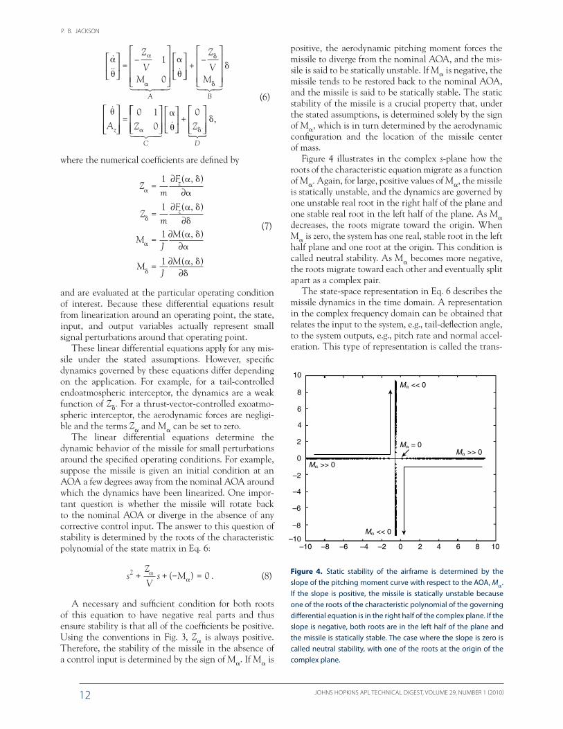
P B JACKSON

JOHNS HOPKINS APL TECHNICAL DIGEST VOLUME 29 NUMBER 1 (2010)12

1 24 3

amp

amp

ampamp

1 24 34

= minus

Z

VM

A

1

0 + minus

=

Z

VM

A Z

B

z

123

0 10

+

C D

Z4

amp

0

amp

(6)

where the numerical coefficients are defined by

Zm

Zm

MJ

=part

=part

=part

1

MJ

=part

partF( )z

1 partF( )z

1 partM( )

1 partM( )

(7)

and are evaluated at the particular operating condition of interest Because these differential equations result from linearization around an operating point the state input and output variables actually represent small signal perturbations around that operating point

These linear differential equations apply for any mis-sile under the stated assumptions However specific dynamics governed by these equations differ depending on the application For example for a tail-controlled endoatmospheric interceptor the dynamics are a weak function of Zd For a thrust-vector-controlled exoatmo-spheric interceptor the aerodynamic forces are negligi-ble and the terms Za and Ma can be set to zero

The linear differential equations determine the dynamic behavior of the missile for small perturbations around the specified operating conditions For example suppose the missile is given an initial condition at an AOA a few degrees away from the nominal AOA around which the dynamics have been linearized One impor-tant question is whether the missile will rotate back to the nominal AOA or diverge in the absence of any corrective control input The answer to this question of stability is determined by the roots of the characteristic polynomial of the state matrix in Eq 6

s M+ + minus =( )sV

2 0 Z

(8)

A necessary and sufficient condition for both roots of this equation to have negative real parts and thus ensure stability is that all of the coefficients be positive Using the conventions in Fig 3 Za is always positive Therefore the stability of the missile in the absence of a control input is determined by the sign of Ma If Ma is

positive the aerodynamic pitching moment forces the missile to diverge from the nominal AOA and the mis-sile is said to be statically unstable If Ma is negative the missile tends to be restored back to the nominal AOA and the missile is said to be statically stable The static stability of the missile is a crucial property that under the stated assumptions is determined solely by the sign of Ma which is in turn determined by the aerodynamic configuration and the location of the missile center of mass

Figure 4 illustrates in the complex s-plane how the roots of the characteristic equation migrate as a function of Ma Again for large positive values of Ma the missile is statically unstable and the dynamics are governed by one unstable real root in the right half of the plane and one stable real root in the left half of the plane As Ma decreases the roots migrate toward the origin When Ma is zero the system has one real stable root in the left half plane and one root at the origin This condition is called neutral stability As Ma becomes more negative the roots migrate toward each other and eventually split apart as a complex pair

The state-space representation in Eq 6 describes the missile dynamics in the time domain A representation in the complex frequency domain can be obtained that relates the input to the system eg tail-deflection angle to the system outputs eg pitch rate and normal accel-eration This type of representation is called the trans-

1086420ndash2ndash4ndash6ndash8ndash10

10

8

6

4

2

0

ndash2

ndash4

ndash6

ndash8

ndash10

M ltlt 0

M ltlt 0

M gtgt 0

M gtgt 0

M = 0

Figure 4 Static stability of the airframe is determined by the slope of the pitching moment curve with respect to the AOA Ma If the slope is positive the missile is statically unstable because one of the roots of the characteristic polynomial of the governing differential equation is in the right half of the complex plane If the slope is negative both roots are in the left half of the plane and the missile is statically stable The case where the slope is zero is called neutral stability with one of the roots at the origin of the complex plane

MISSILE FLIGHT CONTROL SYSTEMS

JOHNS HOPKINS APL TECHNICAL DIGEST VOLUME 29 NUMBER 1 (2010) 13shyshyshyshy

fer function and can be determined from the state-space model using the formula

H s C sI A B D( ) ( ) = minus +minus1 (9)

where s = s + jv is complex fre-quency and A B C and D are defined in Eq 6

In reality missiles are not con-strained to motion in a single plane Figure 5 shows the relevant vari-ables that describe the missile kine-matics in three dimensions The angle of sideslip (AOS) b is the yaw equivalent to the AOA Together they completely specify how the missile body is oriented relative to its velocity vector The three com-ponents of the missile body angular velocity vector resolved in body-fixed coordinates are denoted p q and r denoting the roll pitch and yaw rate respectively The pitch rate q was denoted as in the dis-cussion above where the motion was constrained to the pitch plane

The equations that govern the dynamics of the missile can be developed by applying the NewtonndashEuler equations of motion The

translational motion can be described in terms of the derivatives of the AOA and the AOS The rotational motion can be described in terms of the angu-lar accelerations and takes a simple form assuming that products of inertia are zero

= minus2 2s t

= minus + minusr p

+ minusc tp qamp minusco an se an tanF

mu

F

murzb xb

cos sec tan t

amp 2 2F

mu

F

muyb xb aan tan tan+

q

tan

(10)

amp

amp

amp

pM

IxIz Iy

Ixqr

qM

IyIx Iz

Iypr

rM

I

xb

yb

zb

= minusminus

= minusminus

=zz

Iy IxIz

pqminusminus

(11)

The lateral components of missile inertial translational acceleration resolved in body-fixed coordinates are

A

F

m

AF

m

zzb

yyb

=

=

(12)

In these equations the forces and moments are resolved in body coordinates with components indicated by the subscripts Though not shown explicitly all of the six components of the force and moment vectors are functions of the state variables and three control inputs eg

Figure 5 This diagram defines quantities used to describe the three-dimensional missile kinematics Two angles are used to orient the missile relative to the velocity vector either AOA and AOS or total AOA and aerodynamic roll angle The components of the missile inertial velocity vector resolved in body-fixed axes are u v and w (not shown) The components of the inertial angular velocity vector resolved in body-fixed coordinates are p q and r The missile orientation in inertial space usually is described via three Euler angles typically in yawndashpitchndashroll sequence (not shown)

q

ryB

zBVM

xB

T

A

= AOA = AOST = Total AOAA = Aerodynamic roll angleVM = Missile velocity vector p = Roll angular body rateq = Pitch angular body rater = Yaw angular body ratexB yB zB = Missile body coordinate axes

p

P B JACKSON

JOHNS HOPKINS APL TECHNICAL DIGEST VOLUME 29 NUMBER 1 (2010)14

F f( p q r )zb p y r= (13)

The dynamic equations together are a coupled fifth-order nonlinear differential equation In situations where the mass properties vary with time such as when a rocket motor is burning propellant the differential equation is time-varying as well

Equations 10ndash12 can be linearized around some operat-ing condition of interest by expanding them in a Taylor series and retaining only the first-order terms The result is a linear time-invariant state-space model with three inputs and five outputs

ampx Ax Buy Cx Du

x

u

y A A

T

T

y z

= += +

=

=

=[ pp q r T]

[ p q r]

[ ]p y r

(14)

As in the planar case the state variables control input variables and output variables represent perturbations around the nominal operating condition

Expanding the model to account for yaw and roll in addition to pitch brings a new set of challenges to the flight control designer Foremost among these in many applications is aerodynamic cross-coupling as the total AOA increases in which case aerodynamic surfaces on the leeward side of the missile become shaded by the fuselage resulting in aerodynamic imbalances The net effect typically results in undesirable motion such as roll moment induced by a change in AOA or pitch moment induced by roll control input The flight control system must compensate for these effects An alternative is to simplify the airframe design to minimize cross-coupling but the airframe must be designed with other factors in mind as well such as maximizing the effective range of the missile Compensating for aerodynamic cross- coupling for some missiles is challenging and often limits the maximum total AOA and hence the maxi-mum lateral acceleration that can be achieved by the flight control system

ActuatorThe missile actuator converts the desired control

command developed by the autopilot into physical motion such as rotation of a tail fin that will effect the desired missile motion Actuators for endoatmospheric missiles typically need to be high-bandwidth devices (significantly higher than the desired bandwidth of the flight control loop itself) that can overcome sig-nificant loads Most actuators are electromechanical with hydraulic actuators being an option in certain applications For early design and analysis the actuator

dynamics are modeled with a second-order transfer func-tion (which does not do justice to the actual complexity of the underlying hardware)

s s+ +

(s)

c

a

a a a

=2

2 22

(s) (15)

Although the actuator often is modeled as a linear system for preliminary design and development it is actually a nonlinear device and care must be taken by the flight control designer not to exceed the hardware capabilities Two critical FOMs for the actuator for many endoatmospheric missiles are its rate and position limits The position limit is an effective limit on the moment that the control input can impart on the airframe which in turn limits the maximum AOA and accelera-tion The rate limit essentially limits how fast the actua-tor can cause the missile to rotate which effectively limits how fast the flight control system can respond to changes in the guidance command The performance of a flight control system that commands the actua-tor to exceed its limits can be degraded particularly if the missile is flying at a condition where it is statically unstable

Inertial Measurement UnitThe IMU measures the missile dynamics for feedback

to the autopilot In most flight control applications the IMU is composed of accelerometers and gyroscopes to measure three components of the missile translational acceleration and three components of missile angular velocity For early design and analysis the IMU dynam-ics often are represented by a second-order transfer function

m m+ +

y s

y s s sm m

m

( )

( )=

2

2 22

(16)

for each rate and acceleration channel Like the actuator the IMU needs to be a high-bandwidth device relative to the desired bandwidth of the flight control loop In some applications other quantities also need to be measured such as the pitch angle for an attitude control system In this case other sensors can be used (eg an inertially stabilized platform) or IMU outputs can feed strapdown navigation equations that are implemented in a digital computer to determine the missile attitude which then is sent to the autopilot as a feedback measurement

The flight control system must be designed such that the missile dynamics do not exceed the dynamic range of the IMU If the IMU saturates the missile will lose its inertial reference and the flight control feedback is corrupted The former may be crucial depending on the specific missile application and the phase of flight The

MISSILE FLIGHT CONTROL SYSTEMS

JOHNS HOPKINS APL TECHNICAL DIGEST VOLUME 29 NUMBER 1 (2010) 15shyshyshyshy

latter may be more problematic if the dynamic range is exceeded for too long particularly if the missile is stati-cally unstable

AutopilotThe autopilot is a set of equations that takes as inputs

the guidance commands and the feedback measure-ments from the IMU and computes the control com-mand as the output As mentioned previously the autopilot must be designed so that the control command does not cause oversaturation of the actuator or the IMU Because the autopilot usually is a set of differen-tial equations computing its output involves integrat-ing signals with respect to time Most modern autopilots are implemented in discrete time on digital computers although analog autopilots are still used The following section describes several types of autopilots that apply in different flight control applications

TYPES OF FLIGHT CONTROL SYSTEMSThe specific type of flight control system that is imple-

mented on a particular missile depends on several factors including the overall system mission and requirements packaging constraints and cost In many applications the type of flight control system changes with different phases of flight For example the system used during the boost phase for a ground- or ship-launched missile could very well differ from the system used during the intercept phase This section provides a brief overview of different types of flight control systems and when they might be used

Acceleration Control SystemOne type of flight control system common in many

endoatmospheric applications is designed to track com-manded acceleration perpendicular to the missile longi-tudinal axis In this system deflection of an aerodynamic

control surface such as a tail fin is the control input and pitch angular rate (q) and acceleration (Az) are measured by the IMU for feedback to the autopilot The control deflection produces a small aerodynamic force on the tail fin but a large moment on the airframe because of its lever arm from the center of mass The induced moment rotates the missile to produce the AOA which in turn produces aerodynamic lift to accelerate the airframe

Figure 6 represents equations that can be imple-mented in the autopilot to develop the commanded con-trol surface deflection angle d based on the commanded acceleration and feedback measurements of achieved acceleration Az and pitch rate q This particular struc-ture can be found in many missile applications but is by no means exclusive As indicated in Fig 6 the error between the commanded and achieved acceleration is used as an input to the inner control loops that control missile pitch rate The pitch rate control loops include integration with respect to time that is implemented in circuitry for an analog autopilot or with numerical difference equations in a computer in a digital auto-pilot The three control gains are selected so that the closed-loop flight control system has the desired speed of response and robustness consistent with other design constraints such as actuator limits The autopilot in Fig 6 is a reasonable starting point for a preliminary design The final implementation would need to include other features such as additional filters to attenuate IMU noise and missile vibrations so that the system would actually work in flight and not just on paper

Attitude Control SystemFigure 7 shows another type of autopilot that can

be used to control the attitude of the missile In this case the control effector is the thrust-deflection angle that is actuated by either a nozzle or jet tabs The feed-back loops have a structure similar to that used in the acceleration control system of Fig 6 except that the outer loop is pitch-angle feedback instead of accelera-

Figure 6 This block diagram illustrates a classical approach to the design of an acceleration control autopilot The difference between the scaled input acceleration command and the measured acceleration is multiplied by a gain to effectively form a pitch rate command The difference between the effective pitch rate command and the measured pitch rate is multiplied by a gain and integrated with respect to time The resulting integral is dif-ferenced with the measured pitch rate and multiplied by a third gain to form the control effector command such as desired tail-deflection angle The gain on the input acceleration command ensures zero steady-state error to constant acceleration command inputs The final autopilot design would build on this basic structure with the addition of noise filters and other features such as actuator command limits This basic structure is called the three-loop autopilot

Ki(bull)dtKaKdcAzc

Az

Kr

cActuator

IMU

Airframe dynamics

q

ndash ndash ndash

P B JACKSON

JOHNS HOPKINS APL TECHNICAL DIGEST VOLUME 29 NUMBER 1 (2010)16

tion The numerical values of the gains in the control loops may differ for controlling attitude compared to controlling translational acceleration The inte-gration of pitch rate measured by the IMU to pitch attitude would typically be done via discrete integra-tion in the missile navigation processing in the flight computer

Flight-Path Angle Control SystemFigure 8 shows an autopilot that can be used to track

flight-path angle commands using thrust-vector control This type of system assumes that aerodynamic forces are small and hence applies for exoatmospheric flight or for endoatmospheric flight when the missile speed is low In this design the feedback loops reflect the underly-ing physical relationships among the flight-path angle AOA flight-path angle rate and pitch rate The design explicitly uses estimates of the missile thrust and mass properties to compensate for how the missile dynam-ics change as propellant is expended The commanded input into the autopilot is the desired flight-path angle The output is the thrust-vector deflection angle The feedback signals are the pitch rate q flight-path angle rate g AOA a and flight-path angle g The pitch rate is measured by the IMU The other feedback quantities are estimated in the missile navigation processing in the flight computer This design is an example of the dynamic inversion design approach which will be dis-cussed in Technology Development

FLIGHT CONTROL SYSTEM DESIGN OBJECTIVESThe particular FOMs used to evaluate the flight con-

trol system are application dependent In this section we explore typical FOMs that would generally apply A specific application may include others as well

Time-Domain Design ObjectivesFlight control system FOMs can be expressed in the

time and frequency domains Figure 9 illustrates typi-cal FOMs in the time domain The plot shows the time response of the missile dynamics in response to a step change in commanded input For example this response could represent the achieved missile acceleration in response to a step change in commanded missile accel-eration The time constant and rise time characterize how quickly the system responds to the change in the command The percentage overshoot and peak ampli-tude characterize the degree to which the response is well controlled The steady-state error and settling time are indicators of how well the system tracks the desired command As might be expected designing the flight control system can require trade-offs between these FOMs For example a system that requires a small time constant may have to suffer larger overshoot

In addition to time-domain requirements that mea-sure how well the missile tracks the command in the desired plane of motion the flight control system must be designed to minimize undesirable motion in response to that same command For example the missile should minimize motion in the horizontal plane in response to a guidance command in the vertical plane In other words the flight control system should ldquodecouple the airframerdquo ie compensate for the natural aerodynamic coupling specific to the particular airframe in question Decoupling is important insofar as the derivation of ter-minal guidance laws assumes a perfectly decoupled flight control system

Frequency-Domain Design ObjectivesFrequency-domain requirements are based on the

classical control theory of Nyquist and Bode and are

Figure 7 This attitude control system also has a three-loop struc-ture like the acceleration control system The difference lies in the selection of the numerical values of the gains to reflect a different design criterion ie controlling attitude instead of acceleration

Figure 8 This diagram of a flight-path control system shows the dynamic inversion design approach The design explicitly uses the fundamental relationships among the missile kinematic and dynamic variables as well as real-time estimates of the missile thrust and mass properties to naturally compensate for the changing missile dynamics as propellant is expended

c Ki(bull)dtKa Kr

c

ndash ndash ndash

q(bull)dt

KqKaK

c

c

q

J(TL)ndash ndashndash

mVT

MISSILE FLIGHT CONTROL SYSTEMS

JOHNS HOPKINS APL TECHNICAL DIGEST VOLUME 29 NUMBER 1 (2010) 17shyshyshyshy

Figure 10 The open-loop transfer function at some point of inter-est is computed by ldquobreaking the looprdquo at that point and comput-ing the negative of the transfer function from the resulting input to the output This open-loop transfer function is the bedrock of classical stability analysis in the frequency domain

Output InputK (s) G (s)

ndash

Figure 9 Some basic FOMs of a flight control system that are measured in the time domain are illustrated These FOMs define how quickly the missile will respond to a change in guidance com-mand and also the deviation of the achieved missile motion rela-tive to the command (t is time constant Mp is peak magnitude tp is time to first peak tr is rise time and ts is settling time)

primarily concerned with quantifying the robustness of the flight control system Robustness is important because the flight control system is designed based on models of the missile dynamics actuator and IMU which are inherently approximations (ie no model is perfect) Qualitatively robustness is the degree to which the flight control system can tolerate the error between the assumed models and the real system Robustness can be addressed in several ways two of which are discussed below Classical stability margins quan-tify how much error can be toler-ated at a single point in the system More advanced techniques can be used to quantify robustness to simultaneous variations to mul-tiple parameters in the model

Classical Stability MarginsTwo common measures of

robustness are gain and phase margins as determined by an open-loop frequency response computed at a specific point of interest in the system The open-loop frequency response is computed by break-ing the loop at the point of inter-est and computing the frequency response of the negative of the transfer function from the result-ing input to the resulting output (Fig 10) The gain and phase as a function of frequency often

are plotted separately on what is called a Bode plot Figure 11 is a Bode plot of an example open-loop fre-quency response for an acceleration control system with the loop broken at the input to the actuator The gain margin is determined from the gain curve at the fre-quency where the phase crosses 180deg The gain margin tells how much the gain can be increased or decreased at the loop breakpoint before the closed-loop system becomes unstable The phase margin is determined from the phase curve at the frequency where the gain curve crosses 0 dB The phase margin tells how much extra phase lag ie delay can be tolerated at the loop break-point before the closed-loop system becomes unstable Common requirements for gain and phase margins are 6 dB and 30deg respectively

Mathematically gain and phase margins only apply at the specific point for which they were computed From an engineering standpoint gain and phase varia-tions need to be tolerated at many different points in the system Qualitatively the engineer needs to under-

1Mp

tp

ts

t r

100090

063

050

010

Time

Out

put

0

Figure 11 This Bode plot shows the open-loop frequency response of an acceleration auto-pilot with the loop broken at the input to the actuator In this example the missile is statically unstable which results in the phase curve crossing the 180deg line twice The low-frequency crossover yields a decreasing gain margin (GM) and the high-frequency crossover yields an increasing GM The gain curve crosses the 0-dB line between the phase crossover frequencies resulting in a positive phase margin (PM) At high frequencies the monotonically decreasing gain provides robustness to high-frequency modeling errors uncertainty and other effects

100

50

10310210110010ndash1

0

ndash50

ndash100200

100

0

ndash100

ndash200

Pha

se (

deg)

Mag

nitu

de (

dB)

(rads)

K(s)G(s)

GM1 lt 0

GM2 gt 0

PM gt 0

P B JACKSON

JOHNS HOPKINS APL TECHNICAL DIGEST VOLUME 29 NUMBER 1 (2010)18

stand how all of these variations can be translated to and combined at a single point Consequently designing for good gain and phase margins at a single point is an attempt to cover the net effect of all of the variability in the missile that the flight control system must tolerate Typically gain and phase margins are computed at the input to the actuator and also should be computed at the outputs of the IMU In addition gain and phase margins can be computed at other points in the system that may be of particular interest For example it may be useful to know how much Ma can be increased from its modeled value before the system becomes unstable

The open-loop frequency response at the actuator shown in Fig 11 exhibits characteristics common to a good design At low frequencies the gain is high which is required for good command tracking robustness to low-frequency variations from the modeled system dynamics and rejection of low-frequency disturbances (eg a wind gust or a transient induced by a staging event) At high frequency the gain is small and decreasing which pro-vides attenuation of high-frequency disturbances such as sensor noise and robustness to high-frequency variations to the modeled system dynamics as discussed next

At higher frequencies the concept of gain and phase margins applies mathematically but is not as useful real-istically because the models used for the design and analysis typically become increasingly inaccurate with increasing frequency because of the fundamental non-linear nature of the system Actuators in particular do not behave as linear systems at high frequency because of nonlinearities such as friction and backlash Another issue is that missiles are not perfectly rigid High- frequency flexible body vibrations in response to actua-tor motion can be sensed by the IMU and become a destabilizing effect The net result is that predicted gain and phase values at high frequency can differ consider-ably from their actual values A common approach to address this problem is to ensure that the open-loop gain is below some desired value at all frequencies above some certain lower bound This approach desensitizes the system to high-frequency phase variations The gain requirement is set based on assumptions about the high-frequency modeling errors sometimes based on test data and often comes from hard-learned experi-ence In general the less the designer knows about the actual response of the system (relative to the modeled response) the more conservatism must be built into the design

Not surprisingly such conservatism comes at a cost Gain and phase of a linear system across all frequen-cies must satisfy certain mathematical relationships and cannot be controlled independently Therefore the designer cannot decrease the gain at high frequency without also reducing the phase at lower frequencies which then reduces the phase margin Phase margin can be recovered by modifying the gain to move the 0-dB

Figure 12 This block diagram illustrates a general way to rep-resent the effect of modeling errors or uncertainty in a control system Here w represents the system input (eg an acceleration command) z is the system output (eg achieved acceleration) M(s) is the transfer function model of the nominal system and D represents perturbations to the nominal parameters (eg moment of inertia or aerodynamic coefficients) The model uncertainty can be represented as the gain in a feedback loop around the nominal system Because it is a feedback loop stability of this system can be analyzed using feedback control theory

M(s)

w z

crossover point to lower frequencies but this in turn will likely slow down the step response and increase the time constant Conflicts between high-frequency attenuation requirements and low-frequency bandwidth requirements are not uncommon for a high-performance system particularly with an unstable airframe and can only be solved by giving up one for the other or re-addressing overall system requirements and the system configuration through systems engineering

Robustness to Parameter VariationsSo far the concept of robustness has been addressed

through gain and phase margins which apply at a single point or can be loosely thought of as ldquocoveringrdquo simul-taneous variations and high-frequency attenuation which covers high-frequency modeling errors and uncer-tainty Another type of robustness that can be useful to quantify is tolerance to specific simultaneous parameter variations in the missile dynamics model which is a more accurate error model than assuming that only one parameter can vary while holding the others fixed For example we might wish to know how much variability can be tolerated in Ma and Md simultaneously before the system becomes unstable

This type of problem can be addressed by realizing that it can be viewed within the framework of Fig 12 In Fig 12 the transfer function matrix M(s) represents the nominal closed-loop flight control system where w represents the guidance command (eg commanded acceleration) and z represents the achieved missile dynamics (eg achieved missile acceleration) The feed-back matrix D represents the perturbation to the nomi-nal system In this example D is a 2 3 2 diagonal matrix with the diagonal elements representing the perturba-tions to the nominal values of Ma and Md From the dia-gram it is apparent that perturbations to the nominal system essentially act as an extra feedback loop Hence the question How big can D be before the feedback loop becomes unstable

MISSILE FLIGHT CONTROL SYSTEMS

JOHNS HOPKINS APL TECHNICAL DIGEST VOLUME 29 NUMBER 1 (2010) 19shyshyshyshy

One approach to answering this question is illus-trated in Fig 13 Conceptually a stability boundary is defined by a locus of points in the DMandashDMd plane The goal is to find the minimum distance from the origin to the stability boundary This constrained minimum distance problem can be solved numerically via a gradi-ent projection search1 As with any gradient search the problem of finding local minima must be addressed This approach extends to problems of higher order where the problem is to find the minimum distance from the origin of the perturbation space to an n-dimensional surface that defines the stability boundary

Because the perturbations are really a feedback loop around the nominal system another approach to addressing the simultaneous perturbation problem fol-lows directly from stability theory for multi-input multi-output feedback control systems Using the maximum singular value s for the measure of the magnitude of a matrix the stability problem then is

min( ( )| system is unstable)

s t (17)

ie find the smallest perturbation matrix that destabi-lizes the system The solution to this problem follows from the multivariable Nyquist stability theorem and actually is easily solved assuming that the perturbation matrix D is a fully populated complex matrix when in reality it is a real diagonal matrix Hence this approach tends to be conservative In practice much of the con-servatism can be reduced by specifying in the minimiza-

tion problem that the perturbation matrix has a specific structure

min( ( )| system is unstable

s t

diagonal matrices) (18)

The additional constraint on the structure of the pertur-bation matrix makes this a much more difficult problem to solve

Although the simultaneous perturbation problem can be solved mathematically the flight control engi-neer still needs to formulate the problem in a meaning-ful way particularly when dealing with perturbations to parameters that can have very different dynamic ranges or even different physical units Hence determining the appropriate scaling on the perturbed parameters is an important first step in these types of problems

PITCH ACCELERATION AUTOPILOT EXAMPLEThis section presents an example of a pitch accel-

eration autopilot design for a tail-controlled missile and illustrates some of the FOMs discussed above

The missile dynamics have been linearized around a nominal operating condition of a 10deg AOA and a missile speed of Mach 3 Evaluating the slopes in Eq 7 insert-ing them into the state-space model and computing the transfer functions in the frequency domain yields

A s ss j

q s

z( ) ( )

( )

=minus

+ plusmn0 2038 34 3

0 56 9 32

2 2

( )

s

s j=

minus ++ plusmn

131 10 56 9 32

(s)

(s)

(19)

The denominator of these transfer functions is the same as the left-hand side of the characteristic equation in Eq 8 At this condition the missile has a stable airframe with a pair of lightly damped complex poles

This example assumes that the tail-fin actuator dynamics can be represented by a second-order transfer function (eg Eq 15) with va = 150 rads and a = 07 The IMU is assumed to be ideal ie the feedback mea-surements are equal to their corresponding true values

The autopilot for this example is the basic three-loop autopilot shown in Fig 6 The autopilot gains are selected to provide a time constant of less than 02 s with minimal overshoot The resulting autopilot gains are Kdc = 11 Ka = 45 Ki = 143 and Kr = ndash037

The achieved missile acceleration in response to a unit-step acceleration command input is shown in Fig 14 The time constant is approximately 018 s and the overshoot is only a few percent The response in Fig 14 shows that the initial acceleration develops in the negative direction before reversing and eventually

Figure 13 The stability of the perturbed system can be repre-sented by regions in the perturbation plane The analysis problem then is to define the stability boundary and the shortest distance from it to the origin This problem can be solved with a projected gradient search This solution approach extends to more than two perturbations and can even be used with complex perturbations that represent changes in both gain and phase at critical points in the system

M

M

Stable region

Unstable region

P B JACKSON

JOHNS HOPKINS APL TECHNICAL DIGEST VOLUME 29 NUMBER 1 (2010)20

tracking the command This feature is common to tail- controlled missiles The tail must develop a negative force at the aft end of the missile in order to pitch the nose up and develop a positive AOA The initial nega-tive kick by the tail moves the center of gravity in the negative direction before the AOA increases and devel-ops positive lift to accelerate the missile in the desired direction

Figure 15 shows the Bode plot of the open-loop fre-quency response with the loop broken at the actuator The gain and phase margins are indicated on the plot and at first glance appear to meet the classical criteria of 6 dB and 30deg respectively However the true gain and phase margins might be considerably lower once other effects are included in the model such as IMU dynamics and measurement latencies as well as time delays associated with the digital im-plementation of this autopilot in the flight computer The Bode plot also shows another desirable aspect of a good design the gain curve is mono-tonically decreasing at high fre-quencies which provides some robustness against unmodeled high-frequency dynamics such as the aforementioned flexible body vibrations

TECHNOLOGY CHALLENGESIn this section we review the classical approach to

designing missile flight control systems and discuss where improvements are needed as the requirements on the flight control system become more stringent to pace the threat

The classical approach to designing the missile flight control system can be summarized as follows

1 Develop linear models of the actuator and sensor

2 Define the functional form of the autopilot equations

3 Develop a linear model of the missile dynamics at a flight condition of interest

4 Design autopilot gains in the pitch yaw and roll channels assuming an aerodynamically decoupled airframe to meet basic time-domain requirements

5 Design additional compensation for aerodynamic cross-coupling

6 Design additional filters to attenuate sensor noise and flexible body vibrations

7 Assess linear robustness and performance of the fully coupled system

8 Return to 4 if necessary

9 Repeat 3ndash8 for all flight conditions of interest

10 Develop a methodology to smoothly transition from one set of gains to the next as the missile flies through different flight conditions

11 Add nonlinear features such as actuator command limits if necessary

Figure 14 The response to a unit-step input acceleration com-mand for the pitch acceleration control system example is shown This response illustrates the characteristics of a good design such as a small time constant small overshoot and zero steady-state error The initial acceleration in the negative direction is common to tail-controlled missiles

10080604020

10

12

08

06

04

02

ndash02

0

Time (s)

Acc

eler

atio

n (f

ts2 )

Figure 15 The Bode plot with the loop broken at the actuator input for the example pitch accel-eration control system shows the characteristics of a good design The gain is high at low fre-quency and low at high frequency The stability margins are high These margins will be reduced as other effects are included in the analysis such as IMU dynamics and flight computer process-ing computational delay

GM = 123 dB

Decreasinggain

PM = 44deg

10310210110010ndash1

(rads)

100

0

ndash100200

0

ndash200

Pha

se (

deg)

Mag

nitu

de (

dB)

MISSILE FLIGHT CONTROL SYSTEMS

JOHNS HOPKINS APL TECHNICAL DIGEST VOLUME 29 NUMBER 1 (2010) 21shyshyshyshy

12 Evaluate in a high-fidelity simulation using nonlin-ear aerodynamic actuator and sensor models

13 Return to 3 if necessary

This approach has worked well in the past and will continue to work well in the future for many applica-tions However for high-performance interceptors that need to achieve a high AOA with a small time constant this approach can suffer One potential problem is the separate steps in 4 and 5 for dealing with the aerody-namic coupling Intuitively it might be expected that designing the in-channel and cross-coupling compensa-tion in a unified design approach would yield superior performance Another area for improvement is the way in which the high-fidelity models are used only for assess-ment after the basic design is complete As required time constants decrease the autopilot will likely saturate the actuator for longer periods of time suggesting that non-linear simulation may need to be integral to the design process Further complicating the design is that steps 3ndash8 might need to be carried out for thousands of oper-ating conditions

As the classical design approach evolves the follow-ing challenges need to be addressed

bull The design approach should account for hardware nonlinearities as a fundamental element of the design process

bull The design approach needs to be easily auto-mated so that computer programs can be writ-ten to design the autopilot gains over the entire flight envelope to minimize the need for ldquodesign by handrdquo

bull The design approach should work directly on the fully coupled model of the missile dynamics

bull A good design approach should yield a design that is easily adaptable to changes in the missile configu-ration specifically the mass properties that tend to change over the course of a missile development and production program

Though not explicitly stated any desirable design method should yield a robust control system when prop-erly applied

The first challenge can be addressed by designing the autopilot using numerical optimization programs The cost function that is optimized can include many if not all of the FOMs previously discussed including those from the time-domain response as determined from high-fidelity simulations that include models of the system hardware with their nonlinear dynamics In this way the trade-off between robustness and nonlinear time response is brought directly into the process The challenge then becomes developing a cost function that will meet engineering design goals when it is optimized The last three challenges can be addressed through the

selection of the specific design method to apply to any particular system Many control system design tech-niques are available but finding one method that meets all three of these criteria is difficult APLrsquos contributions in this area are addressed in the next section

APL CONTRIBUTIONSAPL has been involved in the development of flight

control systems for the Navy since the earliest missiles were being developed For many of these programs APL serves as the Technical Direction Agent and as such provides support over the life cycle of a missile program APL also evaluates new theoretical developments in control theory for their applicability to the missile flight control design problem

Life Cycle SupportDuring the concept development phase of a pro-

gram APL is involved in developing the requirements for the flight control system These requirements then flow down to subsystem requirements on the airframe actuator and IMU Typically this subsystem flow-down requires some level of an autopilot design to demonstrate the feasibility of the entire system meeting the flight control requirements

As the missile program proceeds to the development phase APL works closely with the design contractor to ensure a robust design that meets requirements APL develops models independent of the contractor that can be used for model verification and performs an indepen-dent assessment of the design This assessment includes linear analyses as well as predictions from high-fidelity time-domain simulations Parts of the analyses may rep-licate those performed by the contractor to verify results The results of these analyses are communicated back to the contractor with emphasis on areas of concern and potential solutions that may need to be addressed in a subsequent design iteration

As the program progresses to the test-flight phase APL works with the contractor and other organizations to develop test objectives and scenarios The scenarios are designed to maximize coverage over the design space and demonstrate flight control performance with par-ticular emphasis on the time constant and maximum acceleration Along with scenario development are pre-flight predictions based on high-fidelity simulations After the flight APL again conducts an independent postflight analysis and also uses the flight test data for model validation

Technology DevelopmentIn addition to supporting missile development pro-

grams APL has taken an active role in applying new

P B JACKSON

JOHNS HOPKINS APL TECHNICAL DIGEST VOLUME 29 NUMBER 1 (2010)22

theoretical developments in the field of control systems design and assessing their applicability to the missile flight control design problem Our particular emphasis has been on addressing the last three challenges listed previously ie developing design methods that can be automated apply to the fully coupled pitchndashyawndashroll dynamic model and are adaptable to changes in the missile configuration This activity has been ongoing since the earliest Navy missile programs This article covers only the relatively recent activities over the last 20 years or so

In the late 1980s APL demonstrated that the linear quadratic regulator (LQR) theory can be applied to the missile autopilot design problem The LQR design problem is to find the control input that minimizes a quadratic function of the state and control

C x u Ru dtT T= +( ) Qx0

(20)

where x is the vector of state variablesmdasheg AOA AOS etcmdashand u is the vector of control inputsmdasheg pitch yaw and roll tail deflections The constant sym-metric weighting matrices Q and R must be selected to reflect the desired time-domain design criteria such as time constant and overshoot The primary benefit of the LQR approach is that the control solution typi-cally has very good stability margins The difficulty had always been in the appropriate selection of Q and R to represent engineering design criteria APL used the theoretical work of Harvey and Stein2 where Q and R can be constructed to specify a desired eigenstructure of the closed-loop control system The closed-loop eigen-values can be specified based on time-domain require-ments and the eigenvectors can be specified to reflect the desired degree of decoupling between the control channels This approach has been demonstrated to yield robust designs based on the fully coupled dynamic model and can be automated to work on all flight conditions across the battle space It does not however easily adapt to changes in the missile configuration Such changes typically require another iteration of the design over the entire design space

The late 1980s and early 1990s saw an explosion in the use of so-called H design techniques primarily as a result of the groundbreaking solution of the control problem indicated in Fig 163 In the frequency domain the mathematical objective is to find the controller K(s) to compute the control u based on measurements y from the plant P(s) that minimizes the infinity norm of the transfer function matrix that relates the inputs w to the outputs z The infinity norm of a transfer function matrix is defined as

sup (H(j)) = 0rarr

H s( ) = (21)

Loosely speaking the infinity norm is a measure of the maximum gain from input to output over all frequencies

For the flight control application the plant repre-sents the missile dynamics actuator and IMU The controller is the autopilot The control u is the actuator command and the measurements y are the IMU out-puts The inputs w would include for example pitch and yaw acceleration commands and the outputs z would include the pitch and yaw acceleration errors and the missile roll rate The key is that the outputs are not the actual signals themselves but frequency-weighted ver-sions of those signals The frequency-dependent weights map time and frequency-domain design goals to the peak gain over all frequencies of the transfer function from w to z

This approach works well for designing missile auto-pilots at specific operating conditions based on a fully coupled model of the missile dynamics However it results in high-order controllers that may be difficult to implement and it is not easy to automate over the design space APL pioneered the use of this method for the autopilot design problem Some of this work is con-tained in Refs 4ndash9

In the early-to-mid-1990s APL took the lead on the Highly Responsive Missile Control System Advanced Technology Demonstration program This program had several objectives one of which was to demonstrate the efficacy of modern design techniques for the flight con-trol problem and show that the resulting design could be implemented in real time on an embedded processor

P(s)

K(s)

z(s)w(s)

w

yu

z

minK(s)

Figure 16 The H design problem is to find the controller K(s) that minimizes the infinity norm of the transfer function from the inputs in vector w to the outputs in vector z For the flight control design problem the plant P(s) models the actuator airframe and IMU dynamics The controller K(s) is the frequency-domain rep-resentation of the autopilot The inputs w are the guidance com-mands and the outputs z are frequency-weighted signals such as the achieved acceleration The frequency-dependent weights can be chosen to represent typical time-domain and frequency-domain design objectives An approximate solution to this prob-lem can be reached through an iterative approach and involves the solution of two algebraic Riccati equations for each iteration

MISSILE FLIGHT CONTROL SYSTEMS

JOHNS HOPKINS APL TECHNICAL DIGEST VOLUME 29 NUMBER 1 (2010) 23shyshyshyshy

The design method used in this program was based on the normalized co-prime factorization (NCF) approach

In the NCF approach the plant in the frequency domain is viewed in terms of a transfer function numera-tor and denominator (N(s) D(s)) where each has some associated uncertainty as in Fig 17 The control prob-lem is to find the controller K(s) to achieve the desired open-loop frequency response specified by the weight-ing functions W1(s) and W2(s) and simultaneously maxi-mize the size of the uncertainty that would result in an unstable system The weighting functions are specified by the designer as part of the plant model in the design step and then combined with K(s) for implementation Examples using this approach can be found in Ref 10

The NCF approach was shown to yield solid robust designs and could be automated across the design space However a completed design does not readily adapt to changes in the missile configuration Also it does yield high-order controllers that can be difficult to implement Unfortunately the effort was halted before it could be shown that the resulting design could be implemented in real time

In the mid-1990s APL was involved in the analysis of various missile system concepts being proposed for the tactical ballistic missile defense mission To assess these concepts APL developed weapon system simula-tions to evaluate predicted performance Although none of the conceptual systems had actually been designed at this point the Navy nevertheless desired that the simu-lations be of relatively high fidelity To this end APL had to design prototype flight control systems that could be used in high-fidelity nonlinear launch-to-intercept simulations that used fully coupled aerodynamic models These prototype designs had to be developed reasonably quickly be easily modified to adapt to weight and center- of-mass changes to each concept and represent the expected tactical performance of each of these concepts

To this end APL used a technique called nonlinear dynamic inversion to quickly design prototype flight control systems At its core this technique is very simple yet it is a powerful design approach Consider the nonlinear system that is affine in the control input

ampx f x g x u= +( ) ( ) (22)

The control u is to be designed such that the system dynamics follow some desired trajectory that is a func-tion of the state and commanded state

ampx h x xd c= ( ) (23)

A typical form for the desired dynamics is a first- order lag

h x xx x

cc( ) =minus

(24)

with t being the desired time constant These desired dynamics can be achieved through a feedback control law of the form

u g x h x x f xc= minusminus1( )( ( ) ( )) (25)

assuming that the state vector can be measuredFor the acceleration autopilot design problem for

example the dynamic inversion actually is used twice First it is applied to develop control of the missile pitch rate given a desired pitch rate command Once the pitch rate control loop is designed it becomes part of the effec-tive plant for which the outer acceleration control loop is defined using the guidance acceleration command as the reference input

The dynamic inversion design approach is appealing It is a simple concept to understand and apply Because the missile dynamics are explicitly part of the control law it is easily automated and works directly on the non-linear fully coupled pitchndashyawndashroll dynamic model A direct consequence is that the autopilot design naturally adapts to modifications in the missile configuration For example a change to the missile mass properties can be naturally accommodated by updating values in the computations of f(x) and g(x) in Eq 25 whereas for the autopilot shown in Fig 6 the relationship between the values of each gain and the mass properties will not be readily apparent

The primary drawback of the dynamic inversion approach is that is does not provide any theoretical guar-antees of robustness Instead it relies on an experienced designer to specify desired dynamics that can be reason-ably achieved by the airframe and within the bandwidth constraints of the system hardware As with any design

W2(s)W1(s)ndash

PlantDesign plant

K(s)

N(s)+1

D(s)+2

Implemented controller

Figure 17 The normalized co-prime factorization approach uses frequency-dependent weights to shape the open-loop frequency response The design problem is to solve for the controller K(s) to achieve the desired open-loop response and simultaneously max-imize robustness to uncertainty in the numerator and denomina-tor of the transfer function that models the plant dynamics The weights W1(s) and W2(s) are treated as part of the plant for design-ing K(s) and then appended to K(s) for the controller that is imple-mented in the missile software

P B JACKSON

JOHNS HOPKINS APL TECHNICAL DIGEST VOLUME 29 NUMBER 1 (2010)24

approach the final design must be thoroughly assessed in a high-fidelity simulation and through linear analysis techniques

Despite this one drawback the advantages of the dynamic inversion approach make it very appealing In addition the desired dynamics could potentially be made a function of time as well for example to make the missile more responsive as it approaches intercept at short time-to-go The implications of a time-varying design on flight control system performance and on mis-sile performance as a whole are as yet unexplored

CONCLUSIONThis article has covered a variety of topics related

to the missile flight control system The design of this important missile subsystem will continue to evolve to realize the maximum capability of the missile airframe to engage the stressing threats expected in the future

ACKNOWLEDGMENTS G A Harrison and A P Iwaskiw of the APL Guidance Navigation and Control Group pro-vided several helpful inputs for this article

Paul B Jackson is a member of APLrsquos Principal Professional Staff and the supervisor of the Aerodynamic Vehicles Section of the Guidance Navigation and Control Group in the Air and Missile Defense Department He graduated

from Washington University in St Louis in 1988 with a BS degree in systems science and engi-neering and received an MS degree in electrical engineering from The Johns Hopkins Univer-sity in 1992 Since joining APL in 1988 as an engineer in the Guidance Navigation and Control Group Mr Jackson has worked on many aspects of missile guidance and control including autopilot design guidance laws guidance filtering seeker control hardware modeling and simulation devel-opment These activities have spanned a wide variety of programs including Standard Missile-2 Block IIIB Block IV and Block IVA Tomahawk and Standard Missile-6 His e-mail address is pauljacksonjhuapleduPaul B Jackson

The Author

REFERENCES

1Jackson P B ldquoA Gradient Projection Algorithm for Missile Auto-pilot Stability Analysisrdquo in Proc AIAA Guidance Navigation and Control Conf (1992)

2Harvey C and Stein G ldquoQuadratic Weights for Asymptotic Regu-lator Propertiesrdquo IEEE Trans Autom Control AC-23(3) 378ndash387 (June 1978)

3Glover K and Doyle J ldquoState-Space Formulae for All Stabilizing Controllers that Satisfy and H-Infinity Norm Bound and Relations to Risk Sensitivityrdquo Systems Control Lett 11 167ndash172 (1988)

4Reichert R T ldquoApplication of H-Infinity Control to Missile Auto-pilot Designsrdquo in Proc AIAA Guidance Navigation and Control Conf (1989)

5Ruth M J ldquoA Classical Perspective on Application of H-Infinity Control Theory to a Flexible Missile Airframerdquo in Proc AIAA Guid-ance Navigation and Control Conf (1989)

6Jackson P B ldquoApplying m-Synthesis to Missile Autopilot Designrdquo in Proc 29th IEEE Conf on Decision and Control pp 2993ndash2998 (1990)

7Reichert R T ldquoRobust Autopilot Design Using m-Synthesisrdquo in Proc American Control Conf pp 2368ndash2373 (1990)

8Reichert R T ldquoDynamic Scheduling of Modern-Robust-Control Autopilot Designs for Missilesrdquo IEEE Control Systems Magazine 12(5) 35ndash42 (1992)

9Nichols R A Reichert R T and Rugh W J ldquoGain Scheduling for H-Infinity Controllers A Flight Control Examplerdquo IEEE Trans Control Sys Technol 1(2) 69ndash79 (1993)

10 Iglesias P A and Urban T J ldquoLoop Shaping Design of a Missile AutopilotmdashController Configurations and Weighting Filter Selec-tionrdquo in Proc AIAA Guidance Navigation and Control Conf (1999)

The Johns Hopkins APL Technical Digest can be accessed electronically at wwwjhuapledutechdigest

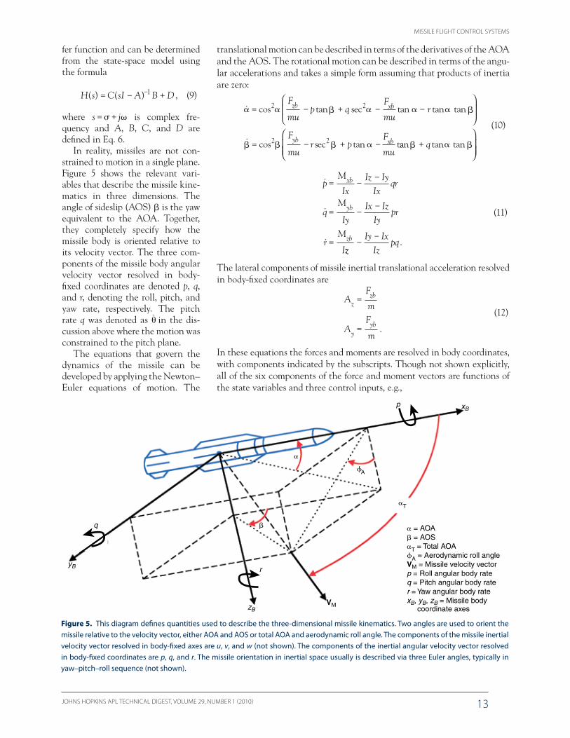
MISSILE FLIGHT CONTROL SYSTEMS

JOHNS HOPKINS APL TECHNICAL DIGEST VOLUME 29 NUMBER 1 (2010) 13shyshyshyshy

fer function and can be determined from the state-space model using the formula

H s C sI A B D( ) ( ) = minus +minus1 (9)

where s = s + jv is complex fre-quency and A B C and D are defined in Eq 6

In reality missiles are not con-strained to motion in a single plane Figure 5 shows the relevant vari-ables that describe the missile kine-matics in three dimensions The angle of sideslip (AOS) b is the yaw equivalent to the AOA Together they completely specify how the missile body is oriented relative to its velocity vector The three com-ponents of the missile body angular velocity vector resolved in body-fixed coordinates are denoted p q and r denoting the roll pitch and yaw rate respectively The pitch rate q was denoted as in the dis-cussion above where the motion was constrained to the pitch plane

The equations that govern the dynamics of the missile can be developed by applying the NewtonndashEuler equations of motion The

translational motion can be described in terms of the derivatives of the AOA and the AOS The rotational motion can be described in terms of the angu-lar accelerations and takes a simple form assuming that products of inertia are zero

= minus2 2s t

= minus + minusr p

+ minusc tp qamp minusco an se an tanF

mu

F

murzb xb

cos sec tan t

amp 2 2F

mu

F

muyb xb aan tan tan+

q

tan

(10)

amp

amp

amp

pM

IxIz Iy

Ixqr

qM

IyIx Iz

Iypr

rM

I

xb

yb

zb

= minusminus

= minusminus

=zz

Iy IxIz

pqminusminus

(11)

The lateral components of missile inertial translational acceleration resolved in body-fixed coordinates are

A

F

m

AF

m

zzb

yyb

=

=

(12)

In these equations the forces and moments are resolved in body coordinates with components indicated by the subscripts Though not shown explicitly all of the six components of the force and moment vectors are functions of the state variables and three control inputs eg

Figure 5 This diagram defines quantities used to describe the three-dimensional missile kinematics Two angles are used to orient the missile relative to the velocity vector either AOA and AOS or total AOA and aerodynamic roll angle The components of the missile inertial velocity vector resolved in body-fixed axes are u v and w (not shown) The components of the inertial angular velocity vector resolved in body-fixed coordinates are p q and r The missile orientation in inertial space usually is described via three Euler angles typically in yawndashpitchndashroll sequence (not shown)

q

ryB

zBVM

xB

T

A

= AOA = AOST = Total AOAA = Aerodynamic roll angleVM = Missile velocity vector p = Roll angular body rateq = Pitch angular body rater = Yaw angular body ratexB yB zB = Missile body coordinate axes

p

P B JACKSON

JOHNS HOPKINS APL TECHNICAL DIGEST VOLUME 29 NUMBER 1 (2010)14

F f( p q r )zb p y r= (13)

The dynamic equations together are a coupled fifth-order nonlinear differential equation In situations where the mass properties vary with time such as when a rocket motor is burning propellant the differential equation is time-varying as well

Equations 10ndash12 can be linearized around some operat-ing condition of interest by expanding them in a Taylor series and retaining only the first-order terms The result is a linear time-invariant state-space model with three inputs and five outputs

ampx Ax Buy Cx Du

x

u

y A A

T

T

y z

= += +

=

=

=[ pp q r T]

[ p q r]

[ ]p y r

(14)

As in the planar case the state variables control input variables and output variables represent perturbations around the nominal operating condition

Expanding the model to account for yaw and roll in addition to pitch brings a new set of challenges to the flight control designer Foremost among these in many applications is aerodynamic cross-coupling as the total AOA increases in which case aerodynamic surfaces on the leeward side of the missile become shaded by the fuselage resulting in aerodynamic imbalances The net effect typically results in undesirable motion such as roll moment induced by a change in AOA or pitch moment induced by roll control input The flight control system must compensate for these effects An alternative is to simplify the airframe design to minimize cross-coupling but the airframe must be designed with other factors in mind as well such as maximizing the effective range of the missile Compensating for aerodynamic cross- coupling for some missiles is challenging and often limits the maximum total AOA and hence the maxi-mum lateral acceleration that can be achieved by the flight control system

ActuatorThe missile actuator converts the desired control

command developed by the autopilot into physical motion such as rotation of a tail fin that will effect the desired missile motion Actuators for endoatmospheric missiles typically need to be high-bandwidth devices (significantly higher than the desired bandwidth of the flight control loop itself) that can overcome sig-nificant loads Most actuators are electromechanical with hydraulic actuators being an option in certain applications For early design and analysis the actuator

dynamics are modeled with a second-order transfer func-tion (which does not do justice to the actual complexity of the underlying hardware)

s s+ +

(s)

c

a

a a a

=2

2 22

(s) (15)

Although the actuator often is modeled as a linear system for preliminary design and development it is actually a nonlinear device and care must be taken by the flight control designer not to exceed the hardware capabilities Two critical FOMs for the actuator for many endoatmospheric missiles are its rate and position limits The position limit is an effective limit on the moment that the control input can impart on the airframe which in turn limits the maximum AOA and accelera-tion The rate limit essentially limits how fast the actua-tor can cause the missile to rotate which effectively limits how fast the flight control system can respond to changes in the guidance command The performance of a flight control system that commands the actua-tor to exceed its limits can be degraded particularly if the missile is flying at a condition where it is statically unstable

Inertial Measurement UnitThe IMU measures the missile dynamics for feedback

to the autopilot In most flight control applications the IMU is composed of accelerometers and gyroscopes to measure three components of the missile translational acceleration and three components of missile angular velocity For early design and analysis the IMU dynam-ics often are represented by a second-order transfer function

m m+ +

y s

y s s sm m

m

( )

( )=

2

2 22

(16)

for each rate and acceleration channel Like the actuator the IMU needs to be a high-bandwidth device relative to the desired bandwidth of the flight control loop In some applications other quantities also need to be measured such as the pitch angle for an attitude control system In this case other sensors can be used (eg an inertially stabilized platform) or IMU outputs can feed strapdown navigation equations that are implemented in a digital computer to determine the missile attitude which then is sent to the autopilot as a feedback measurement

The flight control system must be designed such that the missile dynamics do not exceed the dynamic range of the IMU If the IMU saturates the missile will lose its inertial reference and the flight control feedback is corrupted The former may be crucial depending on the specific missile application and the phase of flight The

MISSILE FLIGHT CONTROL SYSTEMS

JOHNS HOPKINS APL TECHNICAL DIGEST VOLUME 29 NUMBER 1 (2010) 15shyshyshyshy

latter may be more problematic if the dynamic range is exceeded for too long particularly if the missile is stati-cally unstable

AutopilotThe autopilot is a set of equations that takes as inputs

the guidance commands and the feedback measure-ments from the IMU and computes the control com-mand as the output As mentioned previously the autopilot must be designed so that the control command does not cause oversaturation of the actuator or the IMU Because the autopilot usually is a set of differen-tial equations computing its output involves integrat-ing signals with respect to time Most modern autopilots are implemented in discrete time on digital computers although analog autopilots are still used The following section describes several types of autopilots that apply in different flight control applications

TYPES OF FLIGHT CONTROL SYSTEMSThe specific type of flight control system that is imple-

mented on a particular missile depends on several factors including the overall system mission and requirements packaging constraints and cost In many applications the type of flight control system changes with different phases of flight For example the system used during the boost phase for a ground- or ship-launched missile could very well differ from the system used during the intercept phase This section provides a brief overview of different types of flight control systems and when they might be used

Acceleration Control SystemOne type of flight control system common in many

endoatmospheric applications is designed to track com-manded acceleration perpendicular to the missile longi-tudinal axis In this system deflection of an aerodynamic

control surface such as a tail fin is the control input and pitch angular rate (q) and acceleration (Az) are measured by the IMU for feedback to the autopilot The control deflection produces a small aerodynamic force on the tail fin but a large moment on the airframe because of its lever arm from the center of mass The induced moment rotates the missile to produce the AOA which in turn produces aerodynamic lift to accelerate the airframe

Figure 6 represents equations that can be imple-mented in the autopilot to develop the commanded con-trol surface deflection angle d based on the commanded acceleration and feedback measurements of achieved acceleration Az and pitch rate q This particular struc-ture can be found in many missile applications but is by no means exclusive As indicated in Fig 6 the error between the commanded and achieved acceleration is used as an input to the inner control loops that control missile pitch rate The pitch rate control loops include integration with respect to time that is implemented in circuitry for an analog autopilot or with numerical difference equations in a computer in a digital auto-pilot The three control gains are selected so that the closed-loop flight control system has the desired speed of response and robustness consistent with other design constraints such as actuator limits The autopilot in Fig 6 is a reasonable starting point for a preliminary design The final implementation would need to include other features such as additional filters to attenuate IMU noise and missile vibrations so that the system would actually work in flight and not just on paper

Attitude Control SystemFigure 7 shows another type of autopilot that can

be used to control the attitude of the missile In this case the control effector is the thrust-deflection angle that is actuated by either a nozzle or jet tabs The feed-back loops have a structure similar to that used in the acceleration control system of Fig 6 except that the outer loop is pitch-angle feedback instead of accelera-

Figure 6 This block diagram illustrates a classical approach to the design of an acceleration control autopilot The difference between the scaled input acceleration command and the measured acceleration is multiplied by a gain to effectively form a pitch rate command The difference between the effective pitch rate command and the measured pitch rate is multiplied by a gain and integrated with respect to time The resulting integral is dif-ferenced with the measured pitch rate and multiplied by a third gain to form the control effector command such as desired tail-deflection angle The gain on the input acceleration command ensures zero steady-state error to constant acceleration command inputs The final autopilot design would build on this basic structure with the addition of noise filters and other features such as actuator command limits This basic structure is called the three-loop autopilot

Ki(bull)dtKaKdcAzc

Az

Kr

cActuator

IMU

Airframe dynamics

q

ndash ndash ndash

P B JACKSON

JOHNS HOPKINS APL TECHNICAL DIGEST VOLUME 29 NUMBER 1 (2010)16

tion The numerical values of the gains in the control loops may differ for controlling attitude compared to controlling translational acceleration The inte-gration of pitch rate measured by the IMU to pitch attitude would typically be done via discrete integra-tion in the missile navigation processing in the flight computer

Flight-Path Angle Control SystemFigure 8 shows an autopilot that can be used to track

flight-path angle commands using thrust-vector control This type of system assumes that aerodynamic forces are small and hence applies for exoatmospheric flight or for endoatmospheric flight when the missile speed is low In this design the feedback loops reflect the underly-ing physical relationships among the flight-path angle AOA flight-path angle rate and pitch rate The design explicitly uses estimates of the missile thrust and mass properties to compensate for how the missile dynam-ics change as propellant is expended The commanded input into the autopilot is the desired flight-path angle The output is the thrust-vector deflection angle The feedback signals are the pitch rate q flight-path angle rate g AOA a and flight-path angle g The pitch rate is measured by the IMU The other feedback quantities are estimated in the missile navigation processing in the flight computer This design is an example of the dynamic inversion design approach which will be dis-cussed in Technology Development

FLIGHT CONTROL SYSTEM DESIGN OBJECTIVESThe particular FOMs used to evaluate the flight con-

trol system are application dependent In this section we explore typical FOMs that would generally apply A specific application may include others as well

Time-Domain Design ObjectivesFlight control system FOMs can be expressed in the

time and frequency domains Figure 9 illustrates typi-cal FOMs in the time domain The plot shows the time response of the missile dynamics in response to a step change in commanded input For example this response could represent the achieved missile acceleration in response to a step change in commanded missile accel-eration The time constant and rise time characterize how quickly the system responds to the change in the command The percentage overshoot and peak ampli-tude characterize the degree to which the response is well controlled The steady-state error and settling time are indicators of how well the system tracks the desired command As might be expected designing the flight control system can require trade-offs between these FOMs For example a system that requires a small time constant may have to suffer larger overshoot

In addition to time-domain requirements that mea-sure how well the missile tracks the command in the desired plane of motion the flight control system must be designed to minimize undesirable motion in response to that same command For example the missile should minimize motion in the horizontal plane in response to a guidance command in the vertical plane In other words the flight control system should ldquodecouple the airframerdquo ie compensate for the natural aerodynamic coupling specific to the particular airframe in question Decoupling is important insofar as the derivation of ter-minal guidance laws assumes a perfectly decoupled flight control system

Frequency-Domain Design ObjectivesFrequency-domain requirements are based on the

classical control theory of Nyquist and Bode and are

Figure 7 This attitude control system also has a three-loop struc-ture like the acceleration control system The difference lies in the selection of the numerical values of the gains to reflect a different design criterion ie controlling attitude instead of acceleration

Figure 8 This diagram of a flight-path control system shows the dynamic inversion design approach The design explicitly uses the fundamental relationships among the missile kinematic and dynamic variables as well as real-time estimates of the missile thrust and mass properties to naturally compensate for the changing missile dynamics as propellant is expended

c Ki(bull)dtKa Kr

c

ndash ndash ndash

q(bull)dt

KqKaK

c

c

q

J(TL)ndash ndashndash

mVT

MISSILE FLIGHT CONTROL SYSTEMS

JOHNS HOPKINS APL TECHNICAL DIGEST VOLUME 29 NUMBER 1 (2010) 17shyshyshyshy

Figure 10 The open-loop transfer function at some point of inter-est is computed by ldquobreaking the looprdquo at that point and comput-ing the negative of the transfer function from the resulting input to the output This open-loop transfer function is the bedrock of classical stability analysis in the frequency domain

Output InputK (s) G (s)

ndash

Figure 9 Some basic FOMs of a flight control system that are measured in the time domain are illustrated These FOMs define how quickly the missile will respond to a change in guidance com-mand and also the deviation of the achieved missile motion rela-tive to the command (t is time constant Mp is peak magnitude tp is time to first peak tr is rise time and ts is settling time)

primarily concerned with quantifying the robustness of the flight control system Robustness is important because the flight control system is designed based on models of the missile dynamics actuator and IMU which are inherently approximations (ie no model is perfect) Qualitatively robustness is the degree to which the flight control system can tolerate the error between the assumed models and the real system Robustness can be addressed in several ways two of which are discussed below Classical stability margins quan-tify how much error can be toler-ated at a single point in the system More advanced techniques can be used to quantify robustness to simultaneous variations to mul-tiple parameters in the model

Classical Stability MarginsTwo common measures of

robustness are gain and phase margins as determined by an open-loop frequency response computed at a specific point of interest in the system The open-loop frequency response is computed by break-ing the loop at the point of inter-est and computing the frequency response of the negative of the transfer function from the result-ing input to the resulting output (Fig 10) The gain and phase as a function of frequency often

are plotted separately on what is called a Bode plot Figure 11 is a Bode plot of an example open-loop fre-quency response for an acceleration control system with the loop broken at the input to the actuator The gain margin is determined from the gain curve at the fre-quency where the phase crosses 180deg The gain margin tells how much the gain can be increased or decreased at the loop breakpoint before the closed-loop system becomes unstable The phase margin is determined from the phase curve at the frequency where the gain curve crosses 0 dB The phase margin tells how much extra phase lag ie delay can be tolerated at the loop break-point before the closed-loop system becomes unstable Common requirements for gain and phase margins are 6 dB and 30deg respectively

Mathematically gain and phase margins only apply at the specific point for which they were computed From an engineering standpoint gain and phase varia-tions need to be tolerated at many different points in the system Qualitatively the engineer needs to under-

1Mp

tp

ts

t r

100090

063

050

010

Time

Out

put

0

Figure 11 This Bode plot shows the open-loop frequency response of an acceleration auto-pilot with the loop broken at the input to the actuator In this example the missile is statically unstable which results in the phase curve crossing the 180deg line twice The low-frequency crossover yields a decreasing gain margin (GM) and the high-frequency crossover yields an increasing GM The gain curve crosses the 0-dB line between the phase crossover frequencies resulting in a positive phase margin (PM) At high frequencies the monotonically decreasing gain provides robustness to high-frequency modeling errors uncertainty and other effects

100

50

10310210110010ndash1

0

ndash50

ndash100200

100

0

ndash100

ndash200

Pha

se (

deg)

Mag

nitu

de (

dB)

(rads)

K(s)G(s)

GM1 lt 0

GM2 gt 0

PM gt 0

P B JACKSON

JOHNS HOPKINS APL TECHNICAL DIGEST VOLUME 29 NUMBER 1 (2010)18

stand how all of these variations can be translated to and combined at a single point Consequently designing for good gain and phase margins at a single point is an attempt to cover the net effect of all of the variability in the missile that the flight control system must tolerate Typically gain and phase margins are computed at the input to the actuator and also should be computed at the outputs of the IMU In addition gain and phase margins can be computed at other points in the system that may be of particular interest For example it may be useful to know how much Ma can be increased from its modeled value before the system becomes unstable

The open-loop frequency response at the actuator shown in Fig 11 exhibits characteristics common to a good design At low frequencies the gain is high which is required for good command tracking robustness to low-frequency variations from the modeled system dynamics and rejection of low-frequency disturbances (eg a wind gust or a transient induced by a staging event) At high frequency the gain is small and decreasing which pro-vides attenuation of high-frequency disturbances such as sensor noise and robustness to high-frequency variations to the modeled system dynamics as discussed next

At higher frequencies the concept of gain and phase margins applies mathematically but is not as useful real-istically because the models used for the design and analysis typically become increasingly inaccurate with increasing frequency because of the fundamental non-linear nature of the system Actuators in particular do not behave as linear systems at high frequency because of nonlinearities such as friction and backlash Another issue is that missiles are not perfectly rigid High- frequency flexible body vibrations in response to actua-tor motion can be sensed by the IMU and become a destabilizing effect The net result is that predicted gain and phase values at high frequency can differ consider-ably from their actual values A common approach to address this problem is to ensure that the open-loop gain is below some desired value at all frequencies above some certain lower bound This approach desensitizes the system to high-frequency phase variations The gain requirement is set based on assumptions about the high-frequency modeling errors sometimes based on test data and often comes from hard-learned experi-ence In general the less the designer knows about the actual response of the system (relative to the modeled response) the more conservatism must be built into the design

Not surprisingly such conservatism comes at a cost Gain and phase of a linear system across all frequen-cies must satisfy certain mathematical relationships and cannot be controlled independently Therefore the designer cannot decrease the gain at high frequency without also reducing the phase at lower frequencies which then reduces the phase margin Phase margin can be recovered by modifying the gain to move the 0-dB

Figure 12 This block diagram illustrates a general way to rep-resent the effect of modeling errors or uncertainty in a control system Here w represents the system input (eg an acceleration command) z is the system output (eg achieved acceleration) M(s) is the transfer function model of the nominal system and D represents perturbations to the nominal parameters (eg moment of inertia or aerodynamic coefficients) The model uncertainty can be represented as the gain in a feedback loop around the nominal system Because it is a feedback loop stability of this system can be analyzed using feedback control theory

M(s)

w z

crossover point to lower frequencies but this in turn will likely slow down the step response and increase the time constant Conflicts between high-frequency attenuation requirements and low-frequency bandwidth requirements are not uncommon for a high-performance system particularly with an unstable airframe and can only be solved by giving up one for the other or re-addressing overall system requirements and the system configuration through systems engineering

Robustness to Parameter VariationsSo far the concept of robustness has been addressed

through gain and phase margins which apply at a single point or can be loosely thought of as ldquocoveringrdquo simul-taneous variations and high-frequency attenuation which covers high-frequency modeling errors and uncer-tainty Another type of robustness that can be useful to quantify is tolerance to specific simultaneous parameter variations in the missile dynamics model which is a more accurate error model than assuming that only one parameter can vary while holding the others fixed For example we might wish to know how much variability can be tolerated in Ma and Md simultaneously before the system becomes unstable

This type of problem can be addressed by realizing that it can be viewed within the framework of Fig 12 In Fig 12 the transfer function matrix M(s) represents the nominal closed-loop flight control system where w represents the guidance command (eg commanded acceleration) and z represents the achieved missile dynamics (eg achieved missile acceleration) The feed-back matrix D represents the perturbation to the nomi-nal system In this example D is a 2 3 2 diagonal matrix with the diagonal elements representing the perturba-tions to the nominal values of Ma and Md From the dia-gram it is apparent that perturbations to the nominal system essentially act as an extra feedback loop Hence the question How big can D be before the feedback loop becomes unstable

MISSILE FLIGHT CONTROL SYSTEMS

JOHNS HOPKINS APL TECHNICAL DIGEST VOLUME 29 NUMBER 1 (2010) 19shyshyshyshy

One approach to answering this question is illus-trated in Fig 13 Conceptually a stability boundary is defined by a locus of points in the DMandashDMd plane The goal is to find the minimum distance from the origin to the stability boundary This constrained minimum distance problem can be solved numerically via a gradi-ent projection search1 As with any gradient search the problem of finding local minima must be addressed This approach extends to problems of higher order where the problem is to find the minimum distance from the origin of the perturbation space to an n-dimensional surface that defines the stability boundary

Because the perturbations are really a feedback loop around the nominal system another approach to addressing the simultaneous perturbation problem fol-lows directly from stability theory for multi-input multi-output feedback control systems Using the maximum singular value s for the measure of the magnitude of a matrix the stability problem then is

min( ( )| system is unstable)

s t (17)

ie find the smallest perturbation matrix that destabi-lizes the system The solution to this problem follows from the multivariable Nyquist stability theorem and actually is easily solved assuming that the perturbation matrix D is a fully populated complex matrix when in reality it is a real diagonal matrix Hence this approach tends to be conservative In practice much of the con-servatism can be reduced by specifying in the minimiza-

tion problem that the perturbation matrix has a specific structure

min( ( )| system is unstable

s t

diagonal matrices) (18)

The additional constraint on the structure of the pertur-bation matrix makes this a much more difficult problem to solve

Although the simultaneous perturbation problem can be solved mathematically the flight control engi-neer still needs to formulate the problem in a meaning-ful way particularly when dealing with perturbations to parameters that can have very different dynamic ranges or even different physical units Hence determining the appropriate scaling on the perturbed parameters is an important first step in these types of problems

PITCH ACCELERATION AUTOPILOT EXAMPLEThis section presents an example of a pitch accel-

eration autopilot design for a tail-controlled missile and illustrates some of the FOMs discussed above

The missile dynamics have been linearized around a nominal operating condition of a 10deg AOA and a missile speed of Mach 3 Evaluating the slopes in Eq 7 insert-ing them into the state-space model and computing the transfer functions in the frequency domain yields

A s ss j

q s

z( ) ( )

( )

=minus

+ plusmn0 2038 34 3

0 56 9 32

2 2

( )

s

s j=

minus ++ plusmn

131 10 56 9 32

(s)

(s)

(19)

The denominator of these transfer functions is the same as the left-hand side of the characteristic equation in Eq 8 At this condition the missile has a stable airframe with a pair of lightly damped complex poles

This example assumes that the tail-fin actuator dynamics can be represented by a second-order transfer function (eg Eq 15) with va = 150 rads and a = 07 The IMU is assumed to be ideal ie the feedback mea-surements are equal to their corresponding true values

The autopilot for this example is the basic three-loop autopilot shown in Fig 6 The autopilot gains are selected to provide a time constant of less than 02 s with minimal overshoot The resulting autopilot gains are Kdc = 11 Ka = 45 Ki = 143 and Kr = ndash037

The achieved missile acceleration in response to a unit-step acceleration command input is shown in Fig 14 The time constant is approximately 018 s and the overshoot is only a few percent The response in Fig 14 shows that the initial acceleration develops in the negative direction before reversing and eventually

Figure 13 The stability of the perturbed system can be repre-sented by regions in the perturbation plane The analysis problem then is to define the stability boundary and the shortest distance from it to the origin This problem can be solved with a projected gradient search This solution approach extends to more than two perturbations and can even be used with complex perturbations that represent changes in both gain and phase at critical points in the system

M

M

Stable region

Unstable region

P B JACKSON

JOHNS HOPKINS APL TECHNICAL DIGEST VOLUME 29 NUMBER 1 (2010)20

tracking the command This feature is common to tail- controlled missiles The tail must develop a negative force at the aft end of the missile in order to pitch the nose up and develop a positive AOA The initial nega-tive kick by the tail moves the center of gravity in the negative direction before the AOA increases and devel-ops positive lift to accelerate the missile in the desired direction

Figure 15 shows the Bode plot of the open-loop fre-quency response with the loop broken at the actuator The gain and phase margins are indicated on the plot and at first glance appear to meet the classical criteria of 6 dB and 30deg respectively However the true gain and phase margins might be considerably lower once other effects are included in the model such as IMU dynamics and measurement latencies as well as time delays associated with the digital im-plementation of this autopilot in the flight computer The Bode plot also shows another desirable aspect of a good design the gain curve is mono-tonically decreasing at high fre-quencies which provides some robustness against unmodeled high-frequency dynamics such as the aforementioned flexible body vibrations

TECHNOLOGY CHALLENGESIn this section we review the classical approach to

designing missile flight control systems and discuss where improvements are needed as the requirements on the flight control system become more stringent to pace the threat

The classical approach to designing the missile flight control system can be summarized as follows

1 Develop linear models of the actuator and sensor

2 Define the functional form of the autopilot equations

3 Develop a linear model of the missile dynamics at a flight condition of interest

4 Design autopilot gains in the pitch yaw and roll channels assuming an aerodynamically decoupled airframe to meet basic time-domain requirements

5 Design additional compensation for aerodynamic cross-coupling

6 Design additional filters to attenuate sensor noise and flexible body vibrations

7 Assess linear robustness and performance of the fully coupled system

8 Return to 4 if necessary

9 Repeat 3ndash8 for all flight conditions of interest

10 Develop a methodology to smoothly transition from one set of gains to the next as the missile flies through different flight conditions

11 Add nonlinear features such as actuator command limits if necessary

Figure 14 The response to a unit-step input acceleration com-mand for the pitch acceleration control system example is shown This response illustrates the characteristics of a good design such as a small time constant small overshoot and zero steady-state error The initial acceleration in the negative direction is common to tail-controlled missiles

10080604020

10

12

08

06

04

02

ndash02

0

Time (s)

Acc

eler

atio

n (f

ts2 )

Figure 15 The Bode plot with the loop broken at the actuator input for the example pitch accel-eration control system shows the characteristics of a good design The gain is high at low fre-quency and low at high frequency The stability margins are high These margins will be reduced as other effects are included in the analysis such as IMU dynamics and flight computer process-ing computational delay

GM = 123 dB

Decreasinggain

PM = 44deg

10310210110010ndash1

(rads)

100

0

ndash100200

0

ndash200

Pha

se (

deg)

Mag

nitu

de (

dB)

MISSILE FLIGHT CONTROL SYSTEMS

JOHNS HOPKINS APL TECHNICAL DIGEST VOLUME 29 NUMBER 1 (2010) 21shyshyshyshy

12 Evaluate in a high-fidelity simulation using nonlin-ear aerodynamic actuator and sensor models

13 Return to 3 if necessary

This approach has worked well in the past and will continue to work well in the future for many applica-tions However for high-performance interceptors that need to achieve a high AOA with a small time constant this approach can suffer One potential problem is the separate steps in 4 and 5 for dealing with the aerody-namic coupling Intuitively it might be expected that designing the in-channel and cross-coupling compensa-tion in a unified design approach would yield superior performance Another area for improvement is the way in which the high-fidelity models are used only for assess-ment after the basic design is complete As required time constants decrease the autopilot will likely saturate the actuator for longer periods of time suggesting that non-linear simulation may need to be integral to the design process Further complicating the design is that steps 3ndash8 might need to be carried out for thousands of oper-ating conditions

As the classical design approach evolves the follow-ing challenges need to be addressed

bull The design approach should account for hardware nonlinearities as a fundamental element of the design process

bull The design approach needs to be easily auto-mated so that computer programs can be writ-ten to design the autopilot gains over the entire flight envelope to minimize the need for ldquodesign by handrdquo

bull The design approach should work directly on the fully coupled model of the missile dynamics

bull A good design approach should yield a design that is easily adaptable to changes in the missile configu-ration specifically the mass properties that tend to change over the course of a missile development and production program

Though not explicitly stated any desirable design method should yield a robust control system when prop-erly applied

The first challenge can be addressed by designing the autopilot using numerical optimization programs The cost function that is optimized can include many if not all of the FOMs previously discussed including those from the time-domain response as determined from high-fidelity simulations that include models of the system hardware with their nonlinear dynamics In this way the trade-off between robustness and nonlinear time response is brought directly into the process The challenge then becomes developing a cost function that will meet engineering design goals when it is optimized The last three challenges can be addressed through the

selection of the specific design method to apply to any particular system Many control system design tech-niques are available but finding one method that meets all three of these criteria is difficult APLrsquos contributions in this area are addressed in the next section

APL CONTRIBUTIONSAPL has been involved in the development of flight

control systems for the Navy since the earliest missiles were being developed For many of these programs APL serves as the Technical Direction Agent and as such provides support over the life cycle of a missile program APL also evaluates new theoretical developments in control theory for their applicability to the missile flight control design problem

Life Cycle SupportDuring the concept development phase of a pro-

gram APL is involved in developing the requirements for the flight control system These requirements then flow down to subsystem requirements on the airframe actuator and IMU Typically this subsystem flow-down requires some level of an autopilot design to demonstrate the feasibility of the entire system meeting the flight control requirements

As the missile program proceeds to the development phase APL works closely with the design contractor to ensure a robust design that meets requirements APL develops models independent of the contractor that can be used for model verification and performs an indepen-dent assessment of the design This assessment includes linear analyses as well as predictions from high-fidelity time-domain simulations Parts of the analyses may rep-licate those performed by the contractor to verify results The results of these analyses are communicated back to the contractor with emphasis on areas of concern and potential solutions that may need to be addressed in a subsequent design iteration

As the program progresses to the test-flight phase APL works with the contractor and other organizations to develop test objectives and scenarios The scenarios are designed to maximize coverage over the design space and demonstrate flight control performance with par-ticular emphasis on the time constant and maximum acceleration Along with scenario development are pre-flight predictions based on high-fidelity simulations After the flight APL again conducts an independent postflight analysis and also uses the flight test data for model validation

Technology DevelopmentIn addition to supporting missile development pro-

grams APL has taken an active role in applying new

P B JACKSON

JOHNS HOPKINS APL TECHNICAL DIGEST VOLUME 29 NUMBER 1 (2010)22

theoretical developments in the field of control systems design and assessing their applicability to the missile flight control design problem Our particular emphasis has been on addressing the last three challenges listed previously ie developing design methods that can be automated apply to the fully coupled pitchndashyawndashroll dynamic model and are adaptable to changes in the missile configuration This activity has been ongoing since the earliest Navy missile programs This article covers only the relatively recent activities over the last 20 years or so

In the late 1980s APL demonstrated that the linear quadratic regulator (LQR) theory can be applied to the missile autopilot design problem The LQR design problem is to find the control input that minimizes a quadratic function of the state and control

C x u Ru dtT T= +( ) Qx0

(20)

where x is the vector of state variablesmdasheg AOA AOS etcmdashand u is the vector of control inputsmdasheg pitch yaw and roll tail deflections The constant sym-metric weighting matrices Q and R must be selected to reflect the desired time-domain design criteria such as time constant and overshoot The primary benefit of the LQR approach is that the control solution typi-cally has very good stability margins The difficulty had always been in the appropriate selection of Q and R to represent engineering design criteria APL used the theoretical work of Harvey and Stein2 where Q and R can be constructed to specify a desired eigenstructure of the closed-loop control system The closed-loop eigen-values can be specified based on time-domain require-ments and the eigenvectors can be specified to reflect the desired degree of decoupling between the control channels This approach has been demonstrated to yield robust designs based on the fully coupled dynamic model and can be automated to work on all flight conditions across the battle space It does not however easily adapt to changes in the missile configuration Such changes typically require another iteration of the design over the entire design space

The late 1980s and early 1990s saw an explosion in the use of so-called H design techniques primarily as a result of the groundbreaking solution of the control problem indicated in Fig 163 In the frequency domain the mathematical objective is to find the controller K(s) to compute the control u based on measurements y from the plant P(s) that minimizes the infinity norm of the transfer function matrix that relates the inputs w to the outputs z The infinity norm of a transfer function matrix is defined as

sup (H(j)) = 0rarr

H s( ) = (21)

Loosely speaking the infinity norm is a measure of the maximum gain from input to output over all frequencies

For the flight control application the plant repre-sents the missile dynamics actuator and IMU The controller is the autopilot The control u is the actuator command and the measurements y are the IMU out-puts The inputs w would include for example pitch and yaw acceleration commands and the outputs z would include the pitch and yaw acceleration errors and the missile roll rate The key is that the outputs are not the actual signals themselves but frequency-weighted ver-sions of those signals The frequency-dependent weights map time and frequency-domain design goals to the peak gain over all frequencies of the transfer function from w to z

This approach works well for designing missile auto-pilots at specific operating conditions based on a fully coupled model of the missile dynamics However it results in high-order controllers that may be difficult to implement and it is not easy to automate over the design space APL pioneered the use of this method for the autopilot design problem Some of this work is con-tained in Refs 4ndash9

In the early-to-mid-1990s APL took the lead on the Highly Responsive Missile Control System Advanced Technology Demonstration program This program had several objectives one of which was to demonstrate the efficacy of modern design techniques for the flight con-trol problem and show that the resulting design could be implemented in real time on an embedded processor

P(s)

K(s)

z(s)w(s)

w

yu

z

minK(s)

Figure 16 The H design problem is to find the controller K(s) that minimizes the infinity norm of the transfer function from the inputs in vector w to the outputs in vector z For the flight control design problem the plant P(s) models the actuator airframe and IMU dynamics The controller K(s) is the frequency-domain rep-resentation of the autopilot The inputs w are the guidance com-mands and the outputs z are frequency-weighted signals such as the achieved acceleration The frequency-dependent weights can be chosen to represent typical time-domain and frequency-domain design objectives An approximate solution to this prob-lem can be reached through an iterative approach and involves the solution of two algebraic Riccati equations for each iteration

MISSILE FLIGHT CONTROL SYSTEMS

JOHNS HOPKINS APL TECHNICAL DIGEST VOLUME 29 NUMBER 1 (2010) 23shyshyshyshy

The design method used in this program was based on the normalized co-prime factorization (NCF) approach

In the NCF approach the plant in the frequency domain is viewed in terms of a transfer function numera-tor and denominator (N(s) D(s)) where each has some associated uncertainty as in Fig 17 The control prob-lem is to find the controller K(s) to achieve the desired open-loop frequency response specified by the weight-ing functions W1(s) and W2(s) and simultaneously maxi-mize the size of the uncertainty that would result in an unstable system The weighting functions are specified by the designer as part of the plant model in the design step and then combined with K(s) for implementation Examples using this approach can be found in Ref 10

The NCF approach was shown to yield solid robust designs and could be automated across the design space However a completed design does not readily adapt to changes in the missile configuration Also it does yield high-order controllers that can be difficult to implement Unfortunately the effort was halted before it could be shown that the resulting design could be implemented in real time

In the mid-1990s APL was involved in the analysis of various missile system concepts being proposed for the tactical ballistic missile defense mission To assess these concepts APL developed weapon system simula-tions to evaluate predicted performance Although none of the conceptual systems had actually been designed at this point the Navy nevertheless desired that the simu-lations be of relatively high fidelity To this end APL had to design prototype flight control systems that could be used in high-fidelity nonlinear launch-to-intercept simulations that used fully coupled aerodynamic models These prototype designs had to be developed reasonably quickly be easily modified to adapt to weight and center- of-mass changes to each concept and represent the expected tactical performance of each of these concepts

To this end APL used a technique called nonlinear dynamic inversion to quickly design prototype flight control systems At its core this technique is very simple yet it is a powerful design approach Consider the nonlinear system that is affine in the control input

ampx f x g x u= +( ) ( ) (22)

The control u is to be designed such that the system dynamics follow some desired trajectory that is a func-tion of the state and commanded state

ampx h x xd c= ( ) (23)

A typical form for the desired dynamics is a first- order lag

h x xx x

cc( ) =minus

(24)

with t being the desired time constant These desired dynamics can be achieved through a feedback control law of the form

u g x h x x f xc= minusminus1( )( ( ) ( )) (25)

assuming that the state vector can be measuredFor the acceleration autopilot design problem for

example the dynamic inversion actually is used twice First it is applied to develop control of the missile pitch rate given a desired pitch rate command Once the pitch rate control loop is designed it becomes part of the effec-tive plant for which the outer acceleration control loop is defined using the guidance acceleration command as the reference input

The dynamic inversion design approach is appealing It is a simple concept to understand and apply Because the missile dynamics are explicitly part of the control law it is easily automated and works directly on the non-linear fully coupled pitchndashyawndashroll dynamic model A direct consequence is that the autopilot design naturally adapts to modifications in the missile configuration For example a change to the missile mass properties can be naturally accommodated by updating values in the computations of f(x) and g(x) in Eq 25 whereas for the autopilot shown in Fig 6 the relationship between the values of each gain and the mass properties will not be readily apparent

The primary drawback of the dynamic inversion approach is that is does not provide any theoretical guar-antees of robustness Instead it relies on an experienced designer to specify desired dynamics that can be reason-ably achieved by the airframe and within the bandwidth constraints of the system hardware As with any design

W2(s)W1(s)ndash

PlantDesign plant

K(s)

N(s)+1

D(s)+2

Implemented controller

Figure 17 The normalized co-prime factorization approach uses frequency-dependent weights to shape the open-loop frequency response The design problem is to solve for the controller K(s) to achieve the desired open-loop response and simultaneously max-imize robustness to uncertainty in the numerator and denomina-tor of the transfer function that models the plant dynamics The weights W1(s) and W2(s) are treated as part of the plant for design-ing K(s) and then appended to K(s) for the controller that is imple-mented in the missile software

P B JACKSON

JOHNS HOPKINS APL TECHNICAL DIGEST VOLUME 29 NUMBER 1 (2010)24

approach the final design must be thoroughly assessed in a high-fidelity simulation and through linear analysis techniques

Despite this one drawback the advantages of the dynamic inversion approach make it very appealing In addition the desired dynamics could potentially be made a function of time as well for example to make the missile more responsive as it approaches intercept at short time-to-go The implications of a time-varying design on flight control system performance and on mis-sile performance as a whole are as yet unexplored

CONCLUSIONThis article has covered a variety of topics related

to the missile flight control system The design of this important missile subsystem will continue to evolve to realize the maximum capability of the missile airframe to engage the stressing threats expected in the future

ACKNOWLEDGMENTS G A Harrison and A P Iwaskiw of the APL Guidance Navigation and Control Group pro-vided several helpful inputs for this article

Paul B Jackson is a member of APLrsquos Principal Professional Staff and the supervisor of the Aerodynamic Vehicles Section of the Guidance Navigation and Control Group in the Air and Missile Defense Department He graduated

from Washington University in St Louis in 1988 with a BS degree in systems science and engi-neering and received an MS degree in electrical engineering from The Johns Hopkins Univer-sity in 1992 Since joining APL in 1988 as an engineer in the Guidance Navigation and Control Group Mr Jackson has worked on many aspects of missile guidance and control including autopilot design guidance laws guidance filtering seeker control hardware modeling and simulation devel-opment These activities have spanned a wide variety of programs including Standard Missile-2 Block IIIB Block IV and Block IVA Tomahawk and Standard Missile-6 His e-mail address is pauljacksonjhuapleduPaul B Jackson

The Author

REFERENCES

1Jackson P B ldquoA Gradient Projection Algorithm for Missile Auto-pilot Stability Analysisrdquo in Proc AIAA Guidance Navigation and Control Conf (1992)

2Harvey C and Stein G ldquoQuadratic Weights for Asymptotic Regu-lator Propertiesrdquo IEEE Trans Autom Control AC-23(3) 378ndash387 (June 1978)

3Glover K and Doyle J ldquoState-Space Formulae for All Stabilizing Controllers that Satisfy and H-Infinity Norm Bound and Relations to Risk Sensitivityrdquo Systems Control Lett 11 167ndash172 (1988)

4Reichert R T ldquoApplication of H-Infinity Control to Missile Auto-pilot Designsrdquo in Proc AIAA Guidance Navigation and Control Conf (1989)

5Ruth M J ldquoA Classical Perspective on Application of H-Infinity Control Theory to a Flexible Missile Airframerdquo in Proc AIAA Guid-ance Navigation and Control Conf (1989)

6Jackson P B ldquoApplying m-Synthesis to Missile Autopilot Designrdquo in Proc 29th IEEE Conf on Decision and Control pp 2993ndash2998 (1990)

7Reichert R T ldquoRobust Autopilot Design Using m-Synthesisrdquo in Proc American Control Conf pp 2368ndash2373 (1990)

8Reichert R T ldquoDynamic Scheduling of Modern-Robust-Control Autopilot Designs for Missilesrdquo IEEE Control Systems Magazine 12(5) 35ndash42 (1992)

9Nichols R A Reichert R T and Rugh W J ldquoGain Scheduling for H-Infinity Controllers A Flight Control Examplerdquo IEEE Trans Control Sys Technol 1(2) 69ndash79 (1993)

10 Iglesias P A and Urban T J ldquoLoop Shaping Design of a Missile AutopilotmdashController Configurations and Weighting Filter Selec-tionrdquo in Proc AIAA Guidance Navigation and Control Conf (1999)

The Johns Hopkins APL Technical Digest can be accessed electronically at wwwjhuapledutechdigest

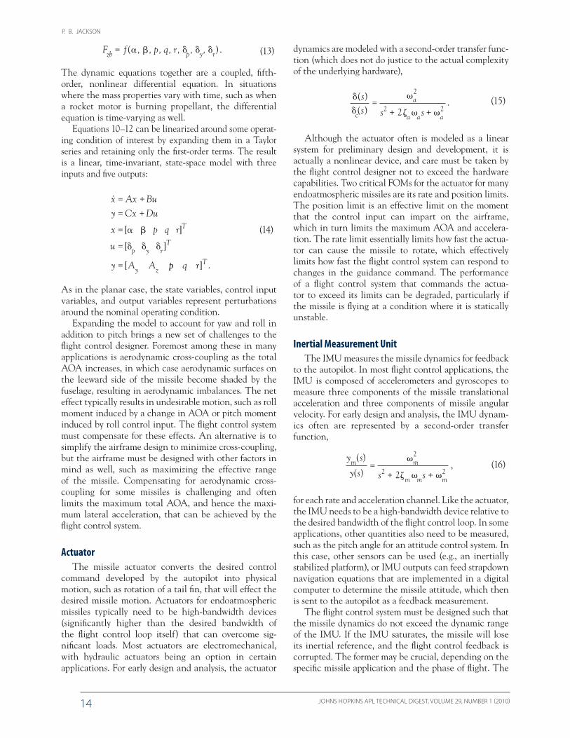
P B JACKSON

JOHNS HOPKINS APL TECHNICAL DIGEST VOLUME 29 NUMBER 1 (2010)14

F f( p q r )zb p y r= (13)

The dynamic equations together are a coupled fifth-order nonlinear differential equation In situations where the mass properties vary with time such as when a rocket motor is burning propellant the differential equation is time-varying as well

Equations 10ndash12 can be linearized around some operat-ing condition of interest by expanding them in a Taylor series and retaining only the first-order terms The result is a linear time-invariant state-space model with three inputs and five outputs

ampx Ax Buy Cx Du

x

u

y A A

T

T

y z

= += +

=

=

=[ pp q r T]

[ p q r]

[ ]p y r

(14)

As in the planar case the state variables control input variables and output variables represent perturbations around the nominal operating condition

Expanding the model to account for yaw and roll in addition to pitch brings a new set of challenges to the flight control designer Foremost among these in many applications is aerodynamic cross-coupling as the total AOA increases in which case aerodynamic surfaces on the leeward side of the missile become shaded by the fuselage resulting in aerodynamic imbalances The net effect typically results in undesirable motion such as roll moment induced by a change in AOA or pitch moment induced by roll control input The flight control system must compensate for these effects An alternative is to simplify the airframe design to minimize cross-coupling but the airframe must be designed with other factors in mind as well such as maximizing the effective range of the missile Compensating for aerodynamic cross- coupling for some missiles is challenging and often limits the maximum total AOA and hence the maxi-mum lateral acceleration that can be achieved by the flight control system

ActuatorThe missile actuator converts the desired control

command developed by the autopilot into physical motion such as rotation of a tail fin that will effect the desired missile motion Actuators for endoatmospheric missiles typically need to be high-bandwidth devices (significantly higher than the desired bandwidth of the flight control loop itself) that can overcome sig-nificant loads Most actuators are electromechanical with hydraulic actuators being an option in certain applications For early design and analysis the actuator

dynamics are modeled with a second-order transfer func-tion (which does not do justice to the actual complexity of the underlying hardware)

s s+ +

(s)

c

a

a a a

=2

2 22

(s) (15)

Although the actuator often is modeled as a linear system for preliminary design and development it is actually a nonlinear device and care must be taken by the flight control designer not to exceed the hardware capabilities Two critical FOMs for the actuator for many endoatmospheric missiles are its rate and position limits The position limit is an effective limit on the moment that the control input can impart on the airframe which in turn limits the maximum AOA and accelera-tion The rate limit essentially limits how fast the actua-tor can cause the missile to rotate which effectively limits how fast the flight control system can respond to changes in the guidance command The performance of a flight control system that commands the actua-tor to exceed its limits can be degraded particularly if the missile is flying at a condition where it is statically unstable

Inertial Measurement UnitThe IMU measures the missile dynamics for feedback

to the autopilot In most flight control applications the IMU is composed of accelerometers and gyroscopes to measure three components of the missile translational acceleration and three components of missile angular velocity For early design and analysis the IMU dynam-ics often are represented by a second-order transfer function

m m+ +

y s

y s s sm m

m

( )

( )=

2

2 22

(16)

for each rate and acceleration channel Like the actuator the IMU needs to be a high-bandwidth device relative to the desired bandwidth of the flight control loop In some applications other quantities also need to be measured such as the pitch angle for an attitude control system In this case other sensors can be used (eg an inertially stabilized platform) or IMU outputs can feed strapdown navigation equations that are implemented in a digital computer to determine the missile attitude which then is sent to the autopilot as a feedback measurement

The flight control system must be designed such that the missile dynamics do not exceed the dynamic range of the IMU If the IMU saturates the missile will lose its inertial reference and the flight control feedback is corrupted The former may be crucial depending on the specific missile application and the phase of flight The

MISSILE FLIGHT CONTROL SYSTEMS

JOHNS HOPKINS APL TECHNICAL DIGEST VOLUME 29 NUMBER 1 (2010) 15shyshyshyshy

latter may be more problematic if the dynamic range is exceeded for too long particularly if the missile is stati-cally unstable

AutopilotThe autopilot is a set of equations that takes as inputs

the guidance commands and the feedback measure-ments from the IMU and computes the control com-mand as the output As mentioned previously the autopilot must be designed so that the control command does not cause oversaturation of the actuator or the IMU Because the autopilot usually is a set of differen-tial equations computing its output involves integrat-ing signals with respect to time Most modern autopilots are implemented in discrete time on digital computers although analog autopilots are still used The following section describes several types of autopilots that apply in different flight control applications

TYPES OF FLIGHT CONTROL SYSTEMSThe specific type of flight control system that is imple-

mented on a particular missile depends on several factors including the overall system mission and requirements packaging constraints and cost In many applications the type of flight control system changes with different phases of flight For example the system used during the boost phase for a ground- or ship-launched missile could very well differ from the system used during the intercept phase This section provides a brief overview of different types of flight control systems and when they might be used

Acceleration Control SystemOne type of flight control system common in many

endoatmospheric applications is designed to track com-manded acceleration perpendicular to the missile longi-tudinal axis In this system deflection of an aerodynamic

control surface such as a tail fin is the control input and pitch angular rate (q) and acceleration (Az) are measured by the IMU for feedback to the autopilot The control deflection produces a small aerodynamic force on the tail fin but a large moment on the airframe because of its lever arm from the center of mass The induced moment rotates the missile to produce the AOA which in turn produces aerodynamic lift to accelerate the airframe

Figure 6 represents equations that can be imple-mented in the autopilot to develop the commanded con-trol surface deflection angle d based on the commanded acceleration and feedback measurements of achieved acceleration Az and pitch rate q This particular struc-ture can be found in many missile applications but is by no means exclusive As indicated in Fig 6 the error between the commanded and achieved acceleration is used as an input to the inner control loops that control missile pitch rate The pitch rate control loops include integration with respect to time that is implemented in circuitry for an analog autopilot or with numerical difference equations in a computer in a digital auto-pilot The three control gains are selected so that the closed-loop flight control system has the desired speed of response and robustness consistent with other design constraints such as actuator limits The autopilot in Fig 6 is a reasonable starting point for a preliminary design The final implementation would need to include other features such as additional filters to attenuate IMU noise and missile vibrations so that the system would actually work in flight and not just on paper

Attitude Control SystemFigure 7 shows another type of autopilot that can

be used to control the attitude of the missile In this case the control effector is the thrust-deflection angle that is actuated by either a nozzle or jet tabs The feed-back loops have a structure similar to that used in the acceleration control system of Fig 6 except that the outer loop is pitch-angle feedback instead of accelera-

Figure 6 This block diagram illustrates a classical approach to the design of an acceleration control autopilot The difference between the scaled input acceleration command and the measured acceleration is multiplied by a gain to effectively form a pitch rate command The difference between the effective pitch rate command and the measured pitch rate is multiplied by a gain and integrated with respect to time The resulting integral is dif-ferenced with the measured pitch rate and multiplied by a third gain to form the control effector command such as desired tail-deflection angle The gain on the input acceleration command ensures zero steady-state error to constant acceleration command inputs The final autopilot design would build on this basic structure with the addition of noise filters and other features such as actuator command limits This basic structure is called the three-loop autopilot

Ki(bull)dtKaKdcAzc

Az

Kr

cActuator

IMU

Airframe dynamics

q

ndash ndash ndash

P B JACKSON

JOHNS HOPKINS APL TECHNICAL DIGEST VOLUME 29 NUMBER 1 (2010)16

tion The numerical values of the gains in the control loops may differ for controlling attitude compared to controlling translational acceleration The inte-gration of pitch rate measured by the IMU to pitch attitude would typically be done via discrete integra-tion in the missile navigation processing in the flight computer

Flight-Path Angle Control SystemFigure 8 shows an autopilot that can be used to track

flight-path angle commands using thrust-vector control This type of system assumes that aerodynamic forces are small and hence applies for exoatmospheric flight or for endoatmospheric flight when the missile speed is low In this design the feedback loops reflect the underly-ing physical relationships among the flight-path angle AOA flight-path angle rate and pitch rate The design explicitly uses estimates of the missile thrust and mass properties to compensate for how the missile dynam-ics change as propellant is expended The commanded input into the autopilot is the desired flight-path angle The output is the thrust-vector deflection angle The feedback signals are the pitch rate q flight-path angle rate g AOA a and flight-path angle g The pitch rate is measured by the IMU The other feedback quantities are estimated in the missile navigation processing in the flight computer This design is an example of the dynamic inversion design approach which will be dis-cussed in Technology Development

FLIGHT CONTROL SYSTEM DESIGN OBJECTIVESThe particular FOMs used to evaluate the flight con-

trol system are application dependent In this section we explore typical FOMs that would generally apply A specific application may include others as well

Time-Domain Design ObjectivesFlight control system FOMs can be expressed in the

time and frequency domains Figure 9 illustrates typi-cal FOMs in the time domain The plot shows the time response of the missile dynamics in response to a step change in commanded input For example this response could represent the achieved missile acceleration in response to a step change in commanded missile accel-eration The time constant and rise time characterize how quickly the system responds to the change in the command The percentage overshoot and peak ampli-tude characterize the degree to which the response is well controlled The steady-state error and settling time are indicators of how well the system tracks the desired command As might be expected designing the flight control system can require trade-offs between these FOMs For example a system that requires a small time constant may have to suffer larger overshoot

In addition to time-domain requirements that mea-sure how well the missile tracks the command in the desired plane of motion the flight control system must be designed to minimize undesirable motion in response to that same command For example the missile should minimize motion in the horizontal plane in response to a guidance command in the vertical plane In other words the flight control system should ldquodecouple the airframerdquo ie compensate for the natural aerodynamic coupling specific to the particular airframe in question Decoupling is important insofar as the derivation of ter-minal guidance laws assumes a perfectly decoupled flight control system

Frequency-Domain Design ObjectivesFrequency-domain requirements are based on the

classical control theory of Nyquist and Bode and are

Figure 7 This attitude control system also has a three-loop struc-ture like the acceleration control system The difference lies in the selection of the numerical values of the gains to reflect a different design criterion ie controlling attitude instead of acceleration

Figure 8 This diagram of a flight-path control system shows the dynamic inversion design approach The design explicitly uses the fundamental relationships among the missile kinematic and dynamic variables as well as real-time estimates of the missile thrust and mass properties to naturally compensate for the changing missile dynamics as propellant is expended

c Ki(bull)dtKa Kr

c

ndash ndash ndash

q(bull)dt

KqKaK

c

c

q

J(TL)ndash ndashndash

mVT

MISSILE FLIGHT CONTROL SYSTEMS

JOHNS HOPKINS APL TECHNICAL DIGEST VOLUME 29 NUMBER 1 (2010) 17shyshyshyshy

Figure 10 The open-loop transfer function at some point of inter-est is computed by ldquobreaking the looprdquo at that point and comput-ing the negative of the transfer function from the resulting input to the output This open-loop transfer function is the bedrock of classical stability analysis in the frequency domain

Output InputK (s) G (s)

ndash

Figure 9 Some basic FOMs of a flight control system that are measured in the time domain are illustrated These FOMs define how quickly the missile will respond to a change in guidance com-mand and also the deviation of the achieved missile motion rela-tive to the command (t is time constant Mp is peak magnitude tp is time to first peak tr is rise time and ts is settling time)

primarily concerned with quantifying the robustness of the flight control system Robustness is important because the flight control system is designed based on models of the missile dynamics actuator and IMU which are inherently approximations (ie no model is perfect) Qualitatively robustness is the degree to which the flight control system can tolerate the error between the assumed models and the real system Robustness can be addressed in several ways two of which are discussed below Classical stability margins quan-tify how much error can be toler-ated at a single point in the system More advanced techniques can be used to quantify robustness to simultaneous variations to mul-tiple parameters in the model

Classical Stability MarginsTwo common measures of

robustness are gain and phase margins as determined by an open-loop frequency response computed at a specific point of interest in the system The open-loop frequency response is computed by break-ing the loop at the point of inter-est and computing the frequency response of the negative of the transfer function from the result-ing input to the resulting output (Fig 10) The gain and phase as a function of frequency often

are plotted separately on what is called a Bode plot Figure 11 is a Bode plot of an example open-loop fre-quency response for an acceleration control system with the loop broken at the input to the actuator The gain margin is determined from the gain curve at the fre-quency where the phase crosses 180deg The gain margin tells how much the gain can be increased or decreased at the loop breakpoint before the closed-loop system becomes unstable The phase margin is determined from the phase curve at the frequency where the gain curve crosses 0 dB The phase margin tells how much extra phase lag ie delay can be tolerated at the loop break-point before the closed-loop system becomes unstable Common requirements for gain and phase margins are 6 dB and 30deg respectively

Mathematically gain and phase margins only apply at the specific point for which they were computed From an engineering standpoint gain and phase varia-tions need to be tolerated at many different points in the system Qualitatively the engineer needs to under-

1Mp

tp

ts

t r

100090

063

050

010

Time

Out

put

0

Figure 11 This Bode plot shows the open-loop frequency response of an acceleration auto-pilot with the loop broken at the input to the actuator In this example the missile is statically unstable which results in the phase curve crossing the 180deg line twice The low-frequency crossover yields a decreasing gain margin (GM) and the high-frequency crossover yields an increasing GM The gain curve crosses the 0-dB line between the phase crossover frequencies resulting in a positive phase margin (PM) At high frequencies the monotonically decreasing gain provides robustness to high-frequency modeling errors uncertainty and other effects

100

50

10310210110010ndash1

0

ndash50

ndash100200

100

0

ndash100

ndash200

Pha

se (

deg)

Mag

nitu

de (

dB)

(rads)

K(s)G(s)

GM1 lt 0

GM2 gt 0

PM gt 0

P B JACKSON

JOHNS HOPKINS APL TECHNICAL DIGEST VOLUME 29 NUMBER 1 (2010)18

stand how all of these variations can be translated to and combined at a single point Consequently designing for good gain and phase margins at a single point is an attempt to cover the net effect of all of the variability in the missile that the flight control system must tolerate Typically gain and phase margins are computed at the input to the actuator and also should be computed at the outputs of the IMU In addition gain and phase margins can be computed at other points in the system that may be of particular interest For example it may be useful to know how much Ma can be increased from its modeled value before the system becomes unstable

The open-loop frequency response at the actuator shown in Fig 11 exhibits characteristics common to a good design At low frequencies the gain is high which is required for good command tracking robustness to low-frequency variations from the modeled system dynamics and rejection of low-frequency disturbances (eg a wind gust or a transient induced by a staging event) At high frequency the gain is small and decreasing which pro-vides attenuation of high-frequency disturbances such as sensor noise and robustness to high-frequency variations to the modeled system dynamics as discussed next

At higher frequencies the concept of gain and phase margins applies mathematically but is not as useful real-istically because the models used for the design and analysis typically become increasingly inaccurate with increasing frequency because of the fundamental non-linear nature of the system Actuators in particular do not behave as linear systems at high frequency because of nonlinearities such as friction and backlash Another issue is that missiles are not perfectly rigid High- frequency flexible body vibrations in response to actua-tor motion can be sensed by the IMU and become a destabilizing effect The net result is that predicted gain and phase values at high frequency can differ consider-ably from their actual values A common approach to address this problem is to ensure that the open-loop gain is below some desired value at all frequencies above some certain lower bound This approach desensitizes the system to high-frequency phase variations The gain requirement is set based on assumptions about the high-frequency modeling errors sometimes based on test data and often comes from hard-learned experi-ence In general the less the designer knows about the actual response of the system (relative to the modeled response) the more conservatism must be built into the design

Not surprisingly such conservatism comes at a cost Gain and phase of a linear system across all frequen-cies must satisfy certain mathematical relationships and cannot be controlled independently Therefore the designer cannot decrease the gain at high frequency without also reducing the phase at lower frequencies which then reduces the phase margin Phase margin can be recovered by modifying the gain to move the 0-dB

Figure 12 This block diagram illustrates a general way to rep-resent the effect of modeling errors or uncertainty in a control system Here w represents the system input (eg an acceleration command) z is the system output (eg achieved acceleration) M(s) is the transfer function model of the nominal system and D represents perturbations to the nominal parameters (eg moment of inertia or aerodynamic coefficients) The model uncertainty can be represented as the gain in a feedback loop around the nominal system Because it is a feedback loop stability of this system can be analyzed using feedback control theory

M(s)

w z

crossover point to lower frequencies but this in turn will likely slow down the step response and increase the time constant Conflicts between high-frequency attenuation requirements and low-frequency bandwidth requirements are not uncommon for a high-performance system particularly with an unstable airframe and can only be solved by giving up one for the other or re-addressing overall system requirements and the system configuration through systems engineering

Robustness to Parameter VariationsSo far the concept of robustness has been addressed

through gain and phase margins which apply at a single point or can be loosely thought of as ldquocoveringrdquo simul-taneous variations and high-frequency attenuation which covers high-frequency modeling errors and uncer-tainty Another type of robustness that can be useful to quantify is tolerance to specific simultaneous parameter variations in the missile dynamics model which is a more accurate error model than assuming that only one parameter can vary while holding the others fixed For example we might wish to know how much variability can be tolerated in Ma and Md simultaneously before the system becomes unstable

This type of problem can be addressed by realizing that it can be viewed within the framework of Fig 12 In Fig 12 the transfer function matrix M(s) represents the nominal closed-loop flight control system where w represents the guidance command (eg commanded acceleration) and z represents the achieved missile dynamics (eg achieved missile acceleration) The feed-back matrix D represents the perturbation to the nomi-nal system In this example D is a 2 3 2 diagonal matrix with the diagonal elements representing the perturba-tions to the nominal values of Ma and Md From the dia-gram it is apparent that perturbations to the nominal system essentially act as an extra feedback loop Hence the question How big can D be before the feedback loop becomes unstable

MISSILE FLIGHT CONTROL SYSTEMS

JOHNS HOPKINS APL TECHNICAL DIGEST VOLUME 29 NUMBER 1 (2010) 19shyshyshyshy

One approach to answering this question is illus-trated in Fig 13 Conceptually a stability boundary is defined by a locus of points in the DMandashDMd plane The goal is to find the minimum distance from the origin to the stability boundary This constrained minimum distance problem can be solved numerically via a gradi-ent projection search1 As with any gradient search the problem of finding local minima must be addressed This approach extends to problems of higher order where the problem is to find the minimum distance from the origin of the perturbation space to an n-dimensional surface that defines the stability boundary

Because the perturbations are really a feedback loop around the nominal system another approach to addressing the simultaneous perturbation problem fol-lows directly from stability theory for multi-input multi-output feedback control systems Using the maximum singular value s for the measure of the magnitude of a matrix the stability problem then is

min( ( )| system is unstable)

s t (17)

ie find the smallest perturbation matrix that destabi-lizes the system The solution to this problem follows from the multivariable Nyquist stability theorem and actually is easily solved assuming that the perturbation matrix D is a fully populated complex matrix when in reality it is a real diagonal matrix Hence this approach tends to be conservative In practice much of the con-servatism can be reduced by specifying in the minimiza-

tion problem that the perturbation matrix has a specific structure

min( ( )| system is unstable

s t

diagonal matrices) (18)

The additional constraint on the structure of the pertur-bation matrix makes this a much more difficult problem to solve

Although the simultaneous perturbation problem can be solved mathematically the flight control engi-neer still needs to formulate the problem in a meaning-ful way particularly when dealing with perturbations to parameters that can have very different dynamic ranges or even different physical units Hence determining the appropriate scaling on the perturbed parameters is an important first step in these types of problems

PITCH ACCELERATION AUTOPILOT EXAMPLEThis section presents an example of a pitch accel-

eration autopilot design for a tail-controlled missile and illustrates some of the FOMs discussed above

The missile dynamics have been linearized around a nominal operating condition of a 10deg AOA and a missile speed of Mach 3 Evaluating the slopes in Eq 7 insert-ing them into the state-space model and computing the transfer functions in the frequency domain yields

A s ss j

q s

z( ) ( )

( )

=minus

+ plusmn0 2038 34 3

0 56 9 32

2 2

( )

s

s j=

minus ++ plusmn

131 10 56 9 32

(s)

(s)

(19)

The denominator of these transfer functions is the same as the left-hand side of the characteristic equation in Eq 8 At this condition the missile has a stable airframe with a pair of lightly damped complex poles

This example assumes that the tail-fin actuator dynamics can be represented by a second-order transfer function (eg Eq 15) with va = 150 rads and a = 07 The IMU is assumed to be ideal ie the feedback mea-surements are equal to their corresponding true values

The autopilot for this example is the basic three-loop autopilot shown in Fig 6 The autopilot gains are selected to provide a time constant of less than 02 s with minimal overshoot The resulting autopilot gains are Kdc = 11 Ka = 45 Ki = 143 and Kr = ndash037

The achieved missile acceleration in response to a unit-step acceleration command input is shown in Fig 14 The time constant is approximately 018 s and the overshoot is only a few percent The response in Fig 14 shows that the initial acceleration develops in the negative direction before reversing and eventually

Figure 13 The stability of the perturbed system can be repre-sented by regions in the perturbation plane The analysis problem then is to define the stability boundary and the shortest distance from it to the origin This problem can be solved with a projected gradient search This solution approach extends to more than two perturbations and can even be used with complex perturbations that represent changes in both gain and phase at critical points in the system

M

M

Stable region

Unstable region

P B JACKSON

JOHNS HOPKINS APL TECHNICAL DIGEST VOLUME 29 NUMBER 1 (2010)20

tracking the command This feature is common to tail- controlled missiles The tail must develop a negative force at the aft end of the missile in order to pitch the nose up and develop a positive AOA The initial nega-tive kick by the tail moves the center of gravity in the negative direction before the AOA increases and devel-ops positive lift to accelerate the missile in the desired direction

Figure 15 shows the Bode plot of the open-loop fre-quency response with the loop broken at the actuator The gain and phase margins are indicated on the plot and at first glance appear to meet the classical criteria of 6 dB and 30deg respectively However the true gain and phase margins might be considerably lower once other effects are included in the model such as IMU dynamics and measurement latencies as well as time delays associated with the digital im-plementation of this autopilot in the flight computer The Bode plot also shows another desirable aspect of a good design the gain curve is mono-tonically decreasing at high fre-quencies which provides some robustness against unmodeled high-frequency dynamics such as the aforementioned flexible body vibrations

TECHNOLOGY CHALLENGESIn this section we review the classical approach to

designing missile flight control systems and discuss where improvements are needed as the requirements on the flight control system become more stringent to pace the threat

The classical approach to designing the missile flight control system can be summarized as follows

1 Develop linear models of the actuator and sensor

2 Define the functional form of the autopilot equations

3 Develop a linear model of the missile dynamics at a flight condition of interest

4 Design autopilot gains in the pitch yaw and roll channels assuming an aerodynamically decoupled airframe to meet basic time-domain requirements

5 Design additional compensation for aerodynamic cross-coupling

6 Design additional filters to attenuate sensor noise and flexible body vibrations

7 Assess linear robustness and performance of the fully coupled system

8 Return to 4 if necessary

9 Repeat 3ndash8 for all flight conditions of interest

10 Develop a methodology to smoothly transition from one set of gains to the next as the missile flies through different flight conditions

11 Add nonlinear features such as actuator command limits if necessary

Figure 14 The response to a unit-step input acceleration com-mand for the pitch acceleration control system example is shown This response illustrates the characteristics of a good design such as a small time constant small overshoot and zero steady-state error The initial acceleration in the negative direction is common to tail-controlled missiles

10080604020

10

12

08

06

04

02

ndash02

0

Time (s)

Acc

eler

atio

n (f

ts2 )

Figure 15 The Bode plot with the loop broken at the actuator input for the example pitch accel-eration control system shows the characteristics of a good design The gain is high at low fre-quency and low at high frequency The stability margins are high These margins will be reduced as other effects are included in the analysis such as IMU dynamics and flight computer process-ing computational delay

GM = 123 dB

Decreasinggain

PM = 44deg

10310210110010ndash1

(rads)

100

0

ndash100200

0

ndash200

Pha

se (

deg)

Mag

nitu

de (

dB)

MISSILE FLIGHT CONTROL SYSTEMS

JOHNS HOPKINS APL TECHNICAL DIGEST VOLUME 29 NUMBER 1 (2010) 21shyshyshyshy

12 Evaluate in a high-fidelity simulation using nonlin-ear aerodynamic actuator and sensor models

13 Return to 3 if necessary

This approach has worked well in the past and will continue to work well in the future for many applica-tions However for high-performance interceptors that need to achieve a high AOA with a small time constant this approach can suffer One potential problem is the separate steps in 4 and 5 for dealing with the aerody-namic coupling Intuitively it might be expected that designing the in-channel and cross-coupling compensa-tion in a unified design approach would yield superior performance Another area for improvement is the way in which the high-fidelity models are used only for assess-ment after the basic design is complete As required time constants decrease the autopilot will likely saturate the actuator for longer periods of time suggesting that non-linear simulation may need to be integral to the design process Further complicating the design is that steps 3ndash8 might need to be carried out for thousands of oper-ating conditions

As the classical design approach evolves the follow-ing challenges need to be addressed

bull The design approach should account for hardware nonlinearities as a fundamental element of the design process

bull The design approach needs to be easily auto-mated so that computer programs can be writ-ten to design the autopilot gains over the entire flight envelope to minimize the need for ldquodesign by handrdquo

bull The design approach should work directly on the fully coupled model of the missile dynamics

bull A good design approach should yield a design that is easily adaptable to changes in the missile configu-ration specifically the mass properties that tend to change over the course of a missile development and production program

Though not explicitly stated any desirable design method should yield a robust control system when prop-erly applied

The first challenge can be addressed by designing the autopilot using numerical optimization programs The cost function that is optimized can include many if not all of the FOMs previously discussed including those from the time-domain response as determined from high-fidelity simulations that include models of the system hardware with their nonlinear dynamics In this way the trade-off between robustness and nonlinear time response is brought directly into the process The challenge then becomes developing a cost function that will meet engineering design goals when it is optimized The last three challenges can be addressed through the

selection of the specific design method to apply to any particular system Many control system design tech-niques are available but finding one method that meets all three of these criteria is difficult APLrsquos contributions in this area are addressed in the next section

APL CONTRIBUTIONSAPL has been involved in the development of flight

control systems for the Navy since the earliest missiles were being developed For many of these programs APL serves as the Technical Direction Agent and as such provides support over the life cycle of a missile program APL also evaluates new theoretical developments in control theory for their applicability to the missile flight control design problem

Life Cycle SupportDuring the concept development phase of a pro-

gram APL is involved in developing the requirements for the flight control system These requirements then flow down to subsystem requirements on the airframe actuator and IMU Typically this subsystem flow-down requires some level of an autopilot design to demonstrate the feasibility of the entire system meeting the flight control requirements

As the missile program proceeds to the development phase APL works closely with the design contractor to ensure a robust design that meets requirements APL develops models independent of the contractor that can be used for model verification and performs an indepen-dent assessment of the design This assessment includes linear analyses as well as predictions from high-fidelity time-domain simulations Parts of the analyses may rep-licate those performed by the contractor to verify results The results of these analyses are communicated back to the contractor with emphasis on areas of concern and potential solutions that may need to be addressed in a subsequent design iteration

As the program progresses to the test-flight phase APL works with the contractor and other organizations to develop test objectives and scenarios The scenarios are designed to maximize coverage over the design space and demonstrate flight control performance with par-ticular emphasis on the time constant and maximum acceleration Along with scenario development are pre-flight predictions based on high-fidelity simulations After the flight APL again conducts an independent postflight analysis and also uses the flight test data for model validation

Technology DevelopmentIn addition to supporting missile development pro-

grams APL has taken an active role in applying new

P B JACKSON

JOHNS HOPKINS APL TECHNICAL DIGEST VOLUME 29 NUMBER 1 (2010)22

theoretical developments in the field of control systems design and assessing their applicability to the missile flight control design problem Our particular emphasis has been on addressing the last three challenges listed previously ie developing design methods that can be automated apply to the fully coupled pitchndashyawndashroll dynamic model and are adaptable to changes in the missile configuration This activity has been ongoing since the earliest Navy missile programs This article covers only the relatively recent activities over the last 20 years or so

In the late 1980s APL demonstrated that the linear quadratic regulator (LQR) theory can be applied to the missile autopilot design problem The LQR design problem is to find the control input that minimizes a quadratic function of the state and control

C x u Ru dtT T= +( ) Qx0

(20)

where x is the vector of state variablesmdasheg AOA AOS etcmdashand u is the vector of control inputsmdasheg pitch yaw and roll tail deflections The constant sym-metric weighting matrices Q and R must be selected to reflect the desired time-domain design criteria such as time constant and overshoot The primary benefit of the LQR approach is that the control solution typi-cally has very good stability margins The difficulty had always been in the appropriate selection of Q and R to represent engineering design criteria APL used the theoretical work of Harvey and Stein2 where Q and R can be constructed to specify a desired eigenstructure of the closed-loop control system The closed-loop eigen-values can be specified based on time-domain require-ments and the eigenvectors can be specified to reflect the desired degree of decoupling between the control channels This approach has been demonstrated to yield robust designs based on the fully coupled dynamic model and can be automated to work on all flight conditions across the battle space It does not however easily adapt to changes in the missile configuration Such changes typically require another iteration of the design over the entire design space

The late 1980s and early 1990s saw an explosion in the use of so-called H design techniques primarily as a result of the groundbreaking solution of the control problem indicated in Fig 163 In the frequency domain the mathematical objective is to find the controller K(s) to compute the control u based on measurements y from the plant P(s) that minimizes the infinity norm of the transfer function matrix that relates the inputs w to the outputs z The infinity norm of a transfer function matrix is defined as

sup (H(j)) = 0rarr

H s( ) = (21)

Loosely speaking the infinity norm is a measure of the maximum gain from input to output over all frequencies

For the flight control application the plant repre-sents the missile dynamics actuator and IMU The controller is the autopilot The control u is the actuator command and the measurements y are the IMU out-puts The inputs w would include for example pitch and yaw acceleration commands and the outputs z would include the pitch and yaw acceleration errors and the missile roll rate The key is that the outputs are not the actual signals themselves but frequency-weighted ver-sions of those signals The frequency-dependent weights map time and frequency-domain design goals to the peak gain over all frequencies of the transfer function from w to z

This approach works well for designing missile auto-pilots at specific operating conditions based on a fully coupled model of the missile dynamics However it results in high-order controllers that may be difficult to implement and it is not easy to automate over the design space APL pioneered the use of this method for the autopilot design problem Some of this work is con-tained in Refs 4ndash9

In the early-to-mid-1990s APL took the lead on the Highly Responsive Missile Control System Advanced Technology Demonstration program This program had several objectives one of which was to demonstrate the efficacy of modern design techniques for the flight con-trol problem and show that the resulting design could be implemented in real time on an embedded processor

P(s)

K(s)

z(s)w(s)

w

yu

z

minK(s)

Figure 16 The H design problem is to find the controller K(s) that minimizes the infinity norm of the transfer function from the inputs in vector w to the outputs in vector z For the flight control design problem the plant P(s) models the actuator airframe and IMU dynamics The controller K(s) is the frequency-domain rep-resentation of the autopilot The inputs w are the guidance com-mands and the outputs z are frequency-weighted signals such as the achieved acceleration The frequency-dependent weights can be chosen to represent typical time-domain and frequency-domain design objectives An approximate solution to this prob-lem can be reached through an iterative approach and involves the solution of two algebraic Riccati equations for each iteration

MISSILE FLIGHT CONTROL SYSTEMS

JOHNS HOPKINS APL TECHNICAL DIGEST VOLUME 29 NUMBER 1 (2010) 23shyshyshyshy

The design method used in this program was based on the normalized co-prime factorization (NCF) approach

In the NCF approach the plant in the frequency domain is viewed in terms of a transfer function numera-tor and denominator (N(s) D(s)) where each has some associated uncertainty as in Fig 17 The control prob-lem is to find the controller K(s) to achieve the desired open-loop frequency response specified by the weight-ing functions W1(s) and W2(s) and simultaneously maxi-mize the size of the uncertainty that would result in an unstable system The weighting functions are specified by the designer as part of the plant model in the design step and then combined with K(s) for implementation Examples using this approach can be found in Ref 10

The NCF approach was shown to yield solid robust designs and could be automated across the design space However a completed design does not readily adapt to changes in the missile configuration Also it does yield high-order controllers that can be difficult to implement Unfortunately the effort was halted before it could be shown that the resulting design could be implemented in real time

In the mid-1990s APL was involved in the analysis of various missile system concepts being proposed for the tactical ballistic missile defense mission To assess these concepts APL developed weapon system simula-tions to evaluate predicted performance Although none of the conceptual systems had actually been designed at this point the Navy nevertheless desired that the simu-lations be of relatively high fidelity To this end APL had to design prototype flight control systems that could be used in high-fidelity nonlinear launch-to-intercept simulations that used fully coupled aerodynamic models These prototype designs had to be developed reasonably quickly be easily modified to adapt to weight and center- of-mass changes to each concept and represent the expected tactical performance of each of these concepts

To this end APL used a technique called nonlinear dynamic inversion to quickly design prototype flight control systems At its core this technique is very simple yet it is a powerful design approach Consider the nonlinear system that is affine in the control input

ampx f x g x u= +( ) ( ) (22)

The control u is to be designed such that the system dynamics follow some desired trajectory that is a func-tion of the state and commanded state

ampx h x xd c= ( ) (23)

A typical form for the desired dynamics is a first- order lag

h x xx x

cc( ) =minus

(24)

with t being the desired time constant These desired dynamics can be achieved through a feedback control law of the form

u g x h x x f xc= minusminus1( )( ( ) ( )) (25)

assuming that the state vector can be measuredFor the acceleration autopilot design problem for

example the dynamic inversion actually is used twice First it is applied to develop control of the missile pitch rate given a desired pitch rate command Once the pitch rate control loop is designed it becomes part of the effec-tive plant for which the outer acceleration control loop is defined using the guidance acceleration command as the reference input

The dynamic inversion design approach is appealing It is a simple concept to understand and apply Because the missile dynamics are explicitly part of the control law it is easily automated and works directly on the non-linear fully coupled pitchndashyawndashroll dynamic model A direct consequence is that the autopilot design naturally adapts to modifications in the missile configuration For example a change to the missile mass properties can be naturally accommodated by updating values in the computations of f(x) and g(x) in Eq 25 whereas for the autopilot shown in Fig 6 the relationship between the values of each gain and the mass properties will not be readily apparent

The primary drawback of the dynamic inversion approach is that is does not provide any theoretical guar-antees of robustness Instead it relies on an experienced designer to specify desired dynamics that can be reason-ably achieved by the airframe and within the bandwidth constraints of the system hardware As with any design

W2(s)W1(s)ndash

PlantDesign plant

K(s)

N(s)+1

D(s)+2

Implemented controller

Figure 17 The normalized co-prime factorization approach uses frequency-dependent weights to shape the open-loop frequency response The design problem is to solve for the controller K(s) to achieve the desired open-loop response and simultaneously max-imize robustness to uncertainty in the numerator and denomina-tor of the transfer function that models the plant dynamics The weights W1(s) and W2(s) are treated as part of the plant for design-ing K(s) and then appended to K(s) for the controller that is imple-mented in the missile software

P B JACKSON

JOHNS HOPKINS APL TECHNICAL DIGEST VOLUME 29 NUMBER 1 (2010)24

approach the final design must be thoroughly assessed in a high-fidelity simulation and through linear analysis techniques

Despite this one drawback the advantages of the dynamic inversion approach make it very appealing In addition the desired dynamics could potentially be made a function of time as well for example to make the missile more responsive as it approaches intercept at short time-to-go The implications of a time-varying design on flight control system performance and on mis-sile performance as a whole are as yet unexplored

CONCLUSIONThis article has covered a variety of topics related

to the missile flight control system The design of this important missile subsystem will continue to evolve to realize the maximum capability of the missile airframe to engage the stressing threats expected in the future

ACKNOWLEDGMENTS G A Harrison and A P Iwaskiw of the APL Guidance Navigation and Control Group pro-vided several helpful inputs for this article

Paul B Jackson is a member of APLrsquos Principal Professional Staff and the supervisor of the Aerodynamic Vehicles Section of the Guidance Navigation and Control Group in the Air and Missile Defense Department He graduated

from Washington University in St Louis in 1988 with a BS degree in systems science and engi-neering and received an MS degree in electrical engineering from The Johns Hopkins Univer-sity in 1992 Since joining APL in 1988 as an engineer in the Guidance Navigation and Control Group Mr Jackson has worked on many aspects of missile guidance and control including autopilot design guidance laws guidance filtering seeker control hardware modeling and simulation devel-opment These activities have spanned a wide variety of programs including Standard Missile-2 Block IIIB Block IV and Block IVA Tomahawk and Standard Missile-6 His e-mail address is pauljacksonjhuapleduPaul B Jackson

The Author

REFERENCES

1Jackson P B ldquoA Gradient Projection Algorithm for Missile Auto-pilot Stability Analysisrdquo in Proc AIAA Guidance Navigation and Control Conf (1992)

2Harvey C and Stein G ldquoQuadratic Weights for Asymptotic Regu-lator Propertiesrdquo IEEE Trans Autom Control AC-23(3) 378ndash387 (June 1978)

3Glover K and Doyle J ldquoState-Space Formulae for All Stabilizing Controllers that Satisfy and H-Infinity Norm Bound and Relations to Risk Sensitivityrdquo Systems Control Lett 11 167ndash172 (1988)

4Reichert R T ldquoApplication of H-Infinity Control to Missile Auto-pilot Designsrdquo in Proc AIAA Guidance Navigation and Control Conf (1989)

5Ruth M J ldquoA Classical Perspective on Application of H-Infinity Control Theory to a Flexible Missile Airframerdquo in Proc AIAA Guid-ance Navigation and Control Conf (1989)

6Jackson P B ldquoApplying m-Synthesis to Missile Autopilot Designrdquo in Proc 29th IEEE Conf on Decision and Control pp 2993ndash2998 (1990)

7Reichert R T ldquoRobust Autopilot Design Using m-Synthesisrdquo in Proc American Control Conf pp 2368ndash2373 (1990)

8Reichert R T ldquoDynamic Scheduling of Modern-Robust-Control Autopilot Designs for Missilesrdquo IEEE Control Systems Magazine 12(5) 35ndash42 (1992)

9Nichols R A Reichert R T and Rugh W J ldquoGain Scheduling for H-Infinity Controllers A Flight Control Examplerdquo IEEE Trans Control Sys Technol 1(2) 69ndash79 (1993)

10 Iglesias P A and Urban T J ldquoLoop Shaping Design of a Missile AutopilotmdashController Configurations and Weighting Filter Selec-tionrdquo in Proc AIAA Guidance Navigation and Control Conf (1999)

The Johns Hopkins APL Technical Digest can be accessed electronically at wwwjhuapledutechdigest

MISSILE FLIGHT CONTROL SYSTEMS

JOHNS HOPKINS APL TECHNICAL DIGEST VOLUME 29 NUMBER 1 (2010) 15shyshyshyshy

latter may be more problematic if the dynamic range is exceeded for too long particularly if the missile is stati-cally unstable

AutopilotThe autopilot is a set of equations that takes as inputs

the guidance commands and the feedback measure-ments from the IMU and computes the control com-mand as the output As mentioned previously the autopilot must be designed so that the control command does not cause oversaturation of the actuator or the IMU Because the autopilot usually is a set of differen-tial equations computing its output involves integrat-ing signals with respect to time Most modern autopilots are implemented in discrete time on digital computers although analog autopilots are still used The following section describes several types of autopilots that apply in different flight control applications

TYPES OF FLIGHT CONTROL SYSTEMSThe specific type of flight control system that is imple-

mented on a particular missile depends on several factors including the overall system mission and requirements packaging constraints and cost In many applications the type of flight control system changes with different phases of flight For example the system used during the boost phase for a ground- or ship-launched missile could very well differ from the system used during the intercept phase This section provides a brief overview of different types of flight control systems and when they might be used

Acceleration Control SystemOne type of flight control system common in many

endoatmospheric applications is designed to track com-manded acceleration perpendicular to the missile longi-tudinal axis In this system deflection of an aerodynamic

control surface such as a tail fin is the control input and pitch angular rate (q) and acceleration (Az) are measured by the IMU for feedback to the autopilot The control deflection produces a small aerodynamic force on the tail fin but a large moment on the airframe because of its lever arm from the center of mass The induced moment rotates the missile to produce the AOA which in turn produces aerodynamic lift to accelerate the airframe

Figure 6 represents equations that can be imple-mented in the autopilot to develop the commanded con-trol surface deflection angle d based on the commanded acceleration and feedback measurements of achieved acceleration Az and pitch rate q This particular struc-ture can be found in many missile applications but is by no means exclusive As indicated in Fig 6 the error between the commanded and achieved acceleration is used as an input to the inner control loops that control missile pitch rate The pitch rate control loops include integration with respect to time that is implemented in circuitry for an analog autopilot or with numerical difference equations in a computer in a digital auto-pilot The three control gains are selected so that the closed-loop flight control system has the desired speed of response and robustness consistent with other design constraints such as actuator limits The autopilot in Fig 6 is a reasonable starting point for a preliminary design The final implementation would need to include other features such as additional filters to attenuate IMU noise and missile vibrations so that the system would actually work in flight and not just on paper

Attitude Control SystemFigure 7 shows another type of autopilot that can

be used to control the attitude of the missile In this case the control effector is the thrust-deflection angle that is actuated by either a nozzle or jet tabs The feed-back loops have a structure similar to that used in the acceleration control system of Fig 6 except that the outer loop is pitch-angle feedback instead of accelera-

Figure 6 This block diagram illustrates a classical approach to the design of an acceleration control autopilot The difference between the scaled input acceleration command and the measured acceleration is multiplied by a gain to effectively form a pitch rate command The difference between the effective pitch rate command and the measured pitch rate is multiplied by a gain and integrated with respect to time The resulting integral is dif-ferenced with the measured pitch rate and multiplied by a third gain to form the control effector command such as desired tail-deflection angle The gain on the input acceleration command ensures zero steady-state error to constant acceleration command inputs The final autopilot design would build on this basic structure with the addition of noise filters and other features such as actuator command limits This basic structure is called the three-loop autopilot

Ki(bull)dtKaKdcAzc

Az

Kr

cActuator

IMU

Airframe dynamics

q

ndash ndash ndash

P B JACKSON

JOHNS HOPKINS APL TECHNICAL DIGEST VOLUME 29 NUMBER 1 (2010)16

tion The numerical values of the gains in the control loops may differ for controlling attitude compared to controlling translational acceleration The inte-gration of pitch rate measured by the IMU to pitch attitude would typically be done via discrete integra-tion in the missile navigation processing in the flight computer

Flight-Path Angle Control SystemFigure 8 shows an autopilot that can be used to track

flight-path angle commands using thrust-vector control This type of system assumes that aerodynamic forces are small and hence applies for exoatmospheric flight or for endoatmospheric flight when the missile speed is low In this design the feedback loops reflect the underly-ing physical relationships among the flight-path angle AOA flight-path angle rate and pitch rate The design explicitly uses estimates of the missile thrust and mass properties to compensate for how the missile dynam-ics change as propellant is expended The commanded input into the autopilot is the desired flight-path angle The output is the thrust-vector deflection angle The feedback signals are the pitch rate q flight-path angle rate g AOA a and flight-path angle g The pitch rate is measured by the IMU The other feedback quantities are estimated in the missile navigation processing in the flight computer This design is an example of the dynamic inversion design approach which will be dis-cussed in Technology Development

FLIGHT CONTROL SYSTEM DESIGN OBJECTIVESThe particular FOMs used to evaluate the flight con-

trol system are application dependent In this section we explore typical FOMs that would generally apply A specific application may include others as well

Time-Domain Design ObjectivesFlight control system FOMs can be expressed in the

time and frequency domains Figure 9 illustrates typi-cal FOMs in the time domain The plot shows the time response of the missile dynamics in response to a step change in commanded input For example this response could represent the achieved missile acceleration in response to a step change in commanded missile accel-eration The time constant and rise time characterize how quickly the system responds to the change in the command The percentage overshoot and peak ampli-tude characterize the degree to which the response is well controlled The steady-state error and settling time are indicators of how well the system tracks the desired command As might be expected designing the flight control system can require trade-offs between these FOMs For example a system that requires a small time constant may have to suffer larger overshoot

In addition to time-domain requirements that mea-sure how well the missile tracks the command in the desired plane of motion the flight control system must be designed to minimize undesirable motion in response to that same command For example the missile should minimize motion in the horizontal plane in response to a guidance command in the vertical plane In other words the flight control system should ldquodecouple the airframerdquo ie compensate for the natural aerodynamic coupling specific to the particular airframe in question Decoupling is important insofar as the derivation of ter-minal guidance laws assumes a perfectly decoupled flight control system

Frequency-Domain Design ObjectivesFrequency-domain requirements are based on the

classical control theory of Nyquist and Bode and are

Figure 7 This attitude control system also has a three-loop struc-ture like the acceleration control system The difference lies in the selection of the numerical values of the gains to reflect a different design criterion ie controlling attitude instead of acceleration

Figure 8 This diagram of a flight-path control system shows the dynamic inversion design approach The design explicitly uses the fundamental relationships among the missile kinematic and dynamic variables as well as real-time estimates of the missile thrust and mass properties to naturally compensate for the changing missile dynamics as propellant is expended

c Ki(bull)dtKa Kr

c

ndash ndash ndash

q(bull)dt

KqKaK

c

c

q

J(TL)ndash ndashndash

mVT

MISSILE FLIGHT CONTROL SYSTEMS

JOHNS HOPKINS APL TECHNICAL DIGEST VOLUME 29 NUMBER 1 (2010) 17shyshyshyshy

Figure 10 The open-loop transfer function at some point of inter-est is computed by ldquobreaking the looprdquo at that point and comput-ing the negative of the transfer function from the resulting input to the output This open-loop transfer function is the bedrock of classical stability analysis in the frequency domain

Output InputK (s) G (s)

ndash

Figure 9 Some basic FOMs of a flight control system that are measured in the time domain are illustrated These FOMs define how quickly the missile will respond to a change in guidance com-mand and also the deviation of the achieved missile motion rela-tive to the command (t is time constant Mp is peak magnitude tp is time to first peak tr is rise time and ts is settling time)

primarily concerned with quantifying the robustness of the flight control system Robustness is important because the flight control system is designed based on models of the missile dynamics actuator and IMU which are inherently approximations (ie no model is perfect) Qualitatively robustness is the degree to which the flight control system can tolerate the error between the assumed models and the real system Robustness can be addressed in several ways two of which are discussed below Classical stability margins quan-tify how much error can be toler-ated at a single point in the system More advanced techniques can be used to quantify robustness to simultaneous variations to mul-tiple parameters in the model

Classical Stability MarginsTwo common measures of

robustness are gain and phase margins as determined by an open-loop frequency response computed at a specific point of interest in the system The open-loop frequency response is computed by break-ing the loop at the point of inter-est and computing the frequency response of the negative of the transfer function from the result-ing input to the resulting output (Fig 10) The gain and phase as a function of frequency often

are plotted separately on what is called a Bode plot Figure 11 is a Bode plot of an example open-loop fre-quency response for an acceleration control system with the loop broken at the input to the actuator The gain margin is determined from the gain curve at the fre-quency where the phase crosses 180deg The gain margin tells how much the gain can be increased or decreased at the loop breakpoint before the closed-loop system becomes unstable The phase margin is determined from the phase curve at the frequency where the gain curve crosses 0 dB The phase margin tells how much extra phase lag ie delay can be tolerated at the loop break-point before the closed-loop system becomes unstable Common requirements for gain and phase margins are 6 dB and 30deg respectively

Mathematically gain and phase margins only apply at the specific point for which they were computed From an engineering standpoint gain and phase varia-tions need to be tolerated at many different points in the system Qualitatively the engineer needs to under-

1Mp

tp

ts

t r

100090

063

050

010

Time

Out

put

0

Figure 11 This Bode plot shows the open-loop frequency response of an acceleration auto-pilot with the loop broken at the input to the actuator In this example the missile is statically unstable which results in the phase curve crossing the 180deg line twice The low-frequency crossover yields a decreasing gain margin (GM) and the high-frequency crossover yields an increasing GM The gain curve crosses the 0-dB line between the phase crossover frequencies resulting in a positive phase margin (PM) At high frequencies the monotonically decreasing gain provides robustness to high-frequency modeling errors uncertainty and other effects

100

50

10310210110010ndash1

0

ndash50

ndash100200

100

0

ndash100

ndash200

Pha

se (

deg)

Mag

nitu

de (

dB)

(rads)

K(s)G(s)

GM1 lt 0

GM2 gt 0

PM gt 0

P B JACKSON

JOHNS HOPKINS APL TECHNICAL DIGEST VOLUME 29 NUMBER 1 (2010)18

stand how all of these variations can be translated to and combined at a single point Consequently designing for good gain and phase margins at a single point is an attempt to cover the net effect of all of the variability in the missile that the flight control system must tolerate Typically gain and phase margins are computed at the input to the actuator and also should be computed at the outputs of the IMU In addition gain and phase margins can be computed at other points in the system that may be of particular interest For example it may be useful to know how much Ma can be increased from its modeled value before the system becomes unstable

The open-loop frequency response at the actuator shown in Fig 11 exhibits characteristics common to a good design At low frequencies the gain is high which is required for good command tracking robustness to low-frequency variations from the modeled system dynamics and rejection of low-frequency disturbances (eg a wind gust or a transient induced by a staging event) At high frequency the gain is small and decreasing which pro-vides attenuation of high-frequency disturbances such as sensor noise and robustness to high-frequency variations to the modeled system dynamics as discussed next

At higher frequencies the concept of gain and phase margins applies mathematically but is not as useful real-istically because the models used for the design and analysis typically become increasingly inaccurate with increasing frequency because of the fundamental non-linear nature of the system Actuators in particular do not behave as linear systems at high frequency because of nonlinearities such as friction and backlash Another issue is that missiles are not perfectly rigid High- frequency flexible body vibrations in response to actua-tor motion can be sensed by the IMU and become a destabilizing effect The net result is that predicted gain and phase values at high frequency can differ consider-ably from their actual values A common approach to address this problem is to ensure that the open-loop gain is below some desired value at all frequencies above some certain lower bound This approach desensitizes the system to high-frequency phase variations The gain requirement is set based on assumptions about the high-frequency modeling errors sometimes based on test data and often comes from hard-learned experi-ence In general the less the designer knows about the actual response of the system (relative to the modeled response) the more conservatism must be built into the design

Not surprisingly such conservatism comes at a cost Gain and phase of a linear system across all frequen-cies must satisfy certain mathematical relationships and cannot be controlled independently Therefore the designer cannot decrease the gain at high frequency without also reducing the phase at lower frequencies which then reduces the phase margin Phase margin can be recovered by modifying the gain to move the 0-dB

Figure 12 This block diagram illustrates a general way to rep-resent the effect of modeling errors or uncertainty in a control system Here w represents the system input (eg an acceleration command) z is the system output (eg achieved acceleration) M(s) is the transfer function model of the nominal system and D represents perturbations to the nominal parameters (eg moment of inertia or aerodynamic coefficients) The model uncertainty can be represented as the gain in a feedback loop around the nominal system Because it is a feedback loop stability of this system can be analyzed using feedback control theory

M(s)

w z

crossover point to lower frequencies but this in turn will likely slow down the step response and increase the time constant Conflicts between high-frequency attenuation requirements and low-frequency bandwidth requirements are not uncommon for a high-performance system particularly with an unstable airframe and can only be solved by giving up one for the other or re-addressing overall system requirements and the system configuration through systems engineering

Robustness to Parameter VariationsSo far the concept of robustness has been addressed

through gain and phase margins which apply at a single point or can be loosely thought of as ldquocoveringrdquo simul-taneous variations and high-frequency attenuation which covers high-frequency modeling errors and uncer-tainty Another type of robustness that can be useful to quantify is tolerance to specific simultaneous parameter variations in the missile dynamics model which is a more accurate error model than assuming that only one parameter can vary while holding the others fixed For example we might wish to know how much variability can be tolerated in Ma and Md simultaneously before the system becomes unstable

This type of problem can be addressed by realizing that it can be viewed within the framework of Fig 12 In Fig 12 the transfer function matrix M(s) represents the nominal closed-loop flight control system where w represents the guidance command (eg commanded acceleration) and z represents the achieved missile dynamics (eg achieved missile acceleration) The feed-back matrix D represents the perturbation to the nomi-nal system In this example D is a 2 3 2 diagonal matrix with the diagonal elements representing the perturba-tions to the nominal values of Ma and Md From the dia-gram it is apparent that perturbations to the nominal system essentially act as an extra feedback loop Hence the question How big can D be before the feedback loop becomes unstable

MISSILE FLIGHT CONTROL SYSTEMS

JOHNS HOPKINS APL TECHNICAL DIGEST VOLUME 29 NUMBER 1 (2010) 19shyshyshyshy

One approach to answering this question is illus-trated in Fig 13 Conceptually a stability boundary is defined by a locus of points in the DMandashDMd plane The goal is to find the minimum distance from the origin to the stability boundary This constrained minimum distance problem can be solved numerically via a gradi-ent projection search1 As with any gradient search the problem of finding local minima must be addressed This approach extends to problems of higher order where the problem is to find the minimum distance from the origin of the perturbation space to an n-dimensional surface that defines the stability boundary

Because the perturbations are really a feedback loop around the nominal system another approach to addressing the simultaneous perturbation problem fol-lows directly from stability theory for multi-input multi-output feedback control systems Using the maximum singular value s for the measure of the magnitude of a matrix the stability problem then is

min( ( )| system is unstable)

s t (17)

ie find the smallest perturbation matrix that destabi-lizes the system The solution to this problem follows from the multivariable Nyquist stability theorem and actually is easily solved assuming that the perturbation matrix D is a fully populated complex matrix when in reality it is a real diagonal matrix Hence this approach tends to be conservative In practice much of the con-servatism can be reduced by specifying in the minimiza-

tion problem that the perturbation matrix has a specific structure

min( ( )| system is unstable

s t

diagonal matrices) (18)

The additional constraint on the structure of the pertur-bation matrix makes this a much more difficult problem to solve

Although the simultaneous perturbation problem can be solved mathematically the flight control engi-neer still needs to formulate the problem in a meaning-ful way particularly when dealing with perturbations to parameters that can have very different dynamic ranges or even different physical units Hence determining the appropriate scaling on the perturbed parameters is an important first step in these types of problems

PITCH ACCELERATION AUTOPILOT EXAMPLEThis section presents an example of a pitch accel-

eration autopilot design for a tail-controlled missile and illustrates some of the FOMs discussed above

The missile dynamics have been linearized around a nominal operating condition of a 10deg AOA and a missile speed of Mach 3 Evaluating the slopes in Eq 7 insert-ing them into the state-space model and computing the transfer functions in the frequency domain yields

A s ss j

q s

z( ) ( )

( )

=minus

+ plusmn0 2038 34 3

0 56 9 32

2 2

( )

s

s j=

minus ++ plusmn

131 10 56 9 32

(s)

(s)

(19)

The denominator of these transfer functions is the same as the left-hand side of the characteristic equation in Eq 8 At this condition the missile has a stable airframe with a pair of lightly damped complex poles

This example assumes that the tail-fin actuator dynamics can be represented by a second-order transfer function (eg Eq 15) with va = 150 rads and a = 07 The IMU is assumed to be ideal ie the feedback mea-surements are equal to their corresponding true values

The autopilot for this example is the basic three-loop autopilot shown in Fig 6 The autopilot gains are selected to provide a time constant of less than 02 s with minimal overshoot The resulting autopilot gains are Kdc = 11 Ka = 45 Ki = 143 and Kr = ndash037

The achieved missile acceleration in response to a unit-step acceleration command input is shown in Fig 14 The time constant is approximately 018 s and the overshoot is only a few percent The response in Fig 14 shows that the initial acceleration develops in the negative direction before reversing and eventually

Figure 13 The stability of the perturbed system can be repre-sented by regions in the perturbation plane The analysis problem then is to define the stability boundary and the shortest distance from it to the origin This problem can be solved with a projected gradient search This solution approach extends to more than two perturbations and can even be used with complex perturbations that represent changes in both gain and phase at critical points in the system

M

M

Stable region

Unstable region

P B JACKSON

JOHNS HOPKINS APL TECHNICAL DIGEST VOLUME 29 NUMBER 1 (2010)20

tracking the command This feature is common to tail- controlled missiles The tail must develop a negative force at the aft end of the missile in order to pitch the nose up and develop a positive AOA The initial nega-tive kick by the tail moves the center of gravity in the negative direction before the AOA increases and devel-ops positive lift to accelerate the missile in the desired direction

Figure 15 shows the Bode plot of the open-loop fre-quency response with the loop broken at the actuator The gain and phase margins are indicated on the plot and at first glance appear to meet the classical criteria of 6 dB and 30deg respectively However the true gain and phase margins might be considerably lower once other effects are included in the model such as IMU dynamics and measurement latencies as well as time delays associated with the digital im-plementation of this autopilot in the flight computer The Bode plot also shows another desirable aspect of a good design the gain curve is mono-tonically decreasing at high fre-quencies which provides some robustness against unmodeled high-frequency dynamics such as the aforementioned flexible body vibrations

TECHNOLOGY CHALLENGESIn this section we review the classical approach to

designing missile flight control systems and discuss where improvements are needed as the requirements on the flight control system become more stringent to pace the threat

The classical approach to designing the missile flight control system can be summarized as follows

1 Develop linear models of the actuator and sensor

2 Define the functional form of the autopilot equations

3 Develop a linear model of the missile dynamics at a flight condition of interest

4 Design autopilot gains in the pitch yaw and roll channels assuming an aerodynamically decoupled airframe to meet basic time-domain requirements

5 Design additional compensation for aerodynamic cross-coupling

6 Design additional filters to attenuate sensor noise and flexible body vibrations

7 Assess linear robustness and performance of the fully coupled system

8 Return to 4 if necessary

9 Repeat 3ndash8 for all flight conditions of interest

10 Develop a methodology to smoothly transition from one set of gains to the next as the missile flies through different flight conditions

11 Add nonlinear features such as actuator command limits if necessary

Figure 14 The response to a unit-step input acceleration com-mand for the pitch acceleration control system example is shown This response illustrates the characteristics of a good design such as a small time constant small overshoot and zero steady-state error The initial acceleration in the negative direction is common to tail-controlled missiles

10080604020

10

12

08

06

04

02

ndash02

0

Time (s)

Acc

eler

atio

n (f

ts2 )

Figure 15 The Bode plot with the loop broken at the actuator input for the example pitch accel-eration control system shows the characteristics of a good design The gain is high at low fre-quency and low at high frequency The stability margins are high These margins will be reduced as other effects are included in the analysis such as IMU dynamics and flight computer process-ing computational delay

GM = 123 dB

Decreasinggain

PM = 44deg

10310210110010ndash1

(rads)

100

0

ndash100200

0

ndash200

Pha

se (

deg)

Mag

nitu

de (

dB)

MISSILE FLIGHT CONTROL SYSTEMS

JOHNS HOPKINS APL TECHNICAL DIGEST VOLUME 29 NUMBER 1 (2010) 21shyshyshyshy

12 Evaluate in a high-fidelity simulation using nonlin-ear aerodynamic actuator and sensor models

13 Return to 3 if necessary

This approach has worked well in the past and will continue to work well in the future for many applica-tions However for high-performance interceptors that need to achieve a high AOA with a small time constant this approach can suffer One potential problem is the separate steps in 4 and 5 for dealing with the aerody-namic coupling Intuitively it might be expected that designing the in-channel and cross-coupling compensa-tion in a unified design approach would yield superior performance Another area for improvement is the way in which the high-fidelity models are used only for assess-ment after the basic design is complete As required time constants decrease the autopilot will likely saturate the actuator for longer periods of time suggesting that non-linear simulation may need to be integral to the design process Further complicating the design is that steps 3ndash8 might need to be carried out for thousands of oper-ating conditions

As the classical design approach evolves the follow-ing challenges need to be addressed

bull The design approach should account for hardware nonlinearities as a fundamental element of the design process

bull The design approach needs to be easily auto-mated so that computer programs can be writ-ten to design the autopilot gains over the entire flight envelope to minimize the need for ldquodesign by handrdquo

bull The design approach should work directly on the fully coupled model of the missile dynamics

bull A good design approach should yield a design that is easily adaptable to changes in the missile configu-ration specifically the mass properties that tend to change over the course of a missile development and production program

Though not explicitly stated any desirable design method should yield a robust control system when prop-erly applied

The first challenge can be addressed by designing the autopilot using numerical optimization programs The cost function that is optimized can include many if not all of the FOMs previously discussed including those from the time-domain response as determined from high-fidelity simulations that include models of the system hardware with their nonlinear dynamics In this way the trade-off between robustness and nonlinear time response is brought directly into the process The challenge then becomes developing a cost function that will meet engineering design goals when it is optimized The last three challenges can be addressed through the

selection of the specific design method to apply to any particular system Many control system design tech-niques are available but finding one method that meets all three of these criteria is difficult APLrsquos contributions in this area are addressed in the next section

APL CONTRIBUTIONSAPL has been involved in the development of flight

control systems for the Navy since the earliest missiles were being developed For many of these programs APL serves as the Technical Direction Agent and as such provides support over the life cycle of a missile program APL also evaluates new theoretical developments in control theory for their applicability to the missile flight control design problem

Life Cycle SupportDuring the concept development phase of a pro-

gram APL is involved in developing the requirements for the flight control system These requirements then flow down to subsystem requirements on the airframe actuator and IMU Typically this subsystem flow-down requires some level of an autopilot design to demonstrate the feasibility of the entire system meeting the flight control requirements

As the missile program proceeds to the development phase APL works closely with the design contractor to ensure a robust design that meets requirements APL develops models independent of the contractor that can be used for model verification and performs an indepen-dent assessment of the design This assessment includes linear analyses as well as predictions from high-fidelity time-domain simulations Parts of the analyses may rep-licate those performed by the contractor to verify results The results of these analyses are communicated back to the contractor with emphasis on areas of concern and potential solutions that may need to be addressed in a subsequent design iteration

As the program progresses to the test-flight phase APL works with the contractor and other organizations to develop test objectives and scenarios The scenarios are designed to maximize coverage over the design space and demonstrate flight control performance with par-ticular emphasis on the time constant and maximum acceleration Along with scenario development are pre-flight predictions based on high-fidelity simulations After the flight APL again conducts an independent postflight analysis and also uses the flight test data for model validation

Technology DevelopmentIn addition to supporting missile development pro-

grams APL has taken an active role in applying new

P B JACKSON

JOHNS HOPKINS APL TECHNICAL DIGEST VOLUME 29 NUMBER 1 (2010)22

theoretical developments in the field of control systems design and assessing their applicability to the missile flight control design problem Our particular emphasis has been on addressing the last three challenges listed previously ie developing design methods that can be automated apply to the fully coupled pitchndashyawndashroll dynamic model and are adaptable to changes in the missile configuration This activity has been ongoing since the earliest Navy missile programs This article covers only the relatively recent activities over the last 20 years or so

In the late 1980s APL demonstrated that the linear quadratic regulator (LQR) theory can be applied to the missile autopilot design problem The LQR design problem is to find the control input that minimizes a quadratic function of the state and control

C x u Ru dtT T= +( ) Qx0

(20)

where x is the vector of state variablesmdasheg AOA AOS etcmdashand u is the vector of control inputsmdasheg pitch yaw and roll tail deflections The constant sym-metric weighting matrices Q and R must be selected to reflect the desired time-domain design criteria such as time constant and overshoot The primary benefit of the LQR approach is that the control solution typi-cally has very good stability margins The difficulty had always been in the appropriate selection of Q and R to represent engineering design criteria APL used the theoretical work of Harvey and Stein2 where Q and R can be constructed to specify a desired eigenstructure of the closed-loop control system The closed-loop eigen-values can be specified based on time-domain require-ments and the eigenvectors can be specified to reflect the desired degree of decoupling between the control channels This approach has been demonstrated to yield robust designs based on the fully coupled dynamic model and can be automated to work on all flight conditions across the battle space It does not however easily adapt to changes in the missile configuration Such changes typically require another iteration of the design over the entire design space

The late 1980s and early 1990s saw an explosion in the use of so-called H design techniques primarily as a result of the groundbreaking solution of the control problem indicated in Fig 163 In the frequency domain the mathematical objective is to find the controller K(s) to compute the control u based on measurements y from the plant P(s) that minimizes the infinity norm of the transfer function matrix that relates the inputs w to the outputs z The infinity norm of a transfer function matrix is defined as

sup (H(j)) = 0rarr

H s( ) = (21)

Loosely speaking the infinity norm is a measure of the maximum gain from input to output over all frequencies

For the flight control application the plant repre-sents the missile dynamics actuator and IMU The controller is the autopilot The control u is the actuator command and the measurements y are the IMU out-puts The inputs w would include for example pitch and yaw acceleration commands and the outputs z would include the pitch and yaw acceleration errors and the missile roll rate The key is that the outputs are not the actual signals themselves but frequency-weighted ver-sions of those signals The frequency-dependent weights map time and frequency-domain design goals to the peak gain over all frequencies of the transfer function from w to z

This approach works well for designing missile auto-pilots at specific operating conditions based on a fully coupled model of the missile dynamics However it results in high-order controllers that may be difficult to implement and it is not easy to automate over the design space APL pioneered the use of this method for the autopilot design problem Some of this work is con-tained in Refs 4ndash9

In the early-to-mid-1990s APL took the lead on the Highly Responsive Missile Control System Advanced Technology Demonstration program This program had several objectives one of which was to demonstrate the efficacy of modern design techniques for the flight con-trol problem and show that the resulting design could be implemented in real time on an embedded processor

P(s)

K(s)

z(s)w(s)

w

yu

z

minK(s)

Figure 16 The H design problem is to find the controller K(s) that minimizes the infinity norm of the transfer function from the inputs in vector w to the outputs in vector z For the flight control design problem the plant P(s) models the actuator airframe and IMU dynamics The controller K(s) is the frequency-domain rep-resentation of the autopilot The inputs w are the guidance com-mands and the outputs z are frequency-weighted signals such as the achieved acceleration The frequency-dependent weights can be chosen to represent typical time-domain and frequency-domain design objectives An approximate solution to this prob-lem can be reached through an iterative approach and involves the solution of two algebraic Riccati equations for each iteration

MISSILE FLIGHT CONTROL SYSTEMS

JOHNS HOPKINS APL TECHNICAL DIGEST VOLUME 29 NUMBER 1 (2010) 23shyshyshyshy

The design method used in this program was based on the normalized co-prime factorization (NCF) approach

In the NCF approach the plant in the frequency domain is viewed in terms of a transfer function numera-tor and denominator (N(s) D(s)) where each has some associated uncertainty as in Fig 17 The control prob-lem is to find the controller K(s) to achieve the desired open-loop frequency response specified by the weight-ing functions W1(s) and W2(s) and simultaneously maxi-mize the size of the uncertainty that would result in an unstable system The weighting functions are specified by the designer as part of the plant model in the design step and then combined with K(s) for implementation Examples using this approach can be found in Ref 10

The NCF approach was shown to yield solid robust designs and could be automated across the design space However a completed design does not readily adapt to changes in the missile configuration Also it does yield high-order controllers that can be difficult to implement Unfortunately the effort was halted before it could be shown that the resulting design could be implemented in real time

In the mid-1990s APL was involved in the analysis of various missile system concepts being proposed for the tactical ballistic missile defense mission To assess these concepts APL developed weapon system simula-tions to evaluate predicted performance Although none of the conceptual systems had actually been designed at this point the Navy nevertheless desired that the simu-lations be of relatively high fidelity To this end APL had to design prototype flight control systems that could be used in high-fidelity nonlinear launch-to-intercept simulations that used fully coupled aerodynamic models These prototype designs had to be developed reasonably quickly be easily modified to adapt to weight and center- of-mass changes to each concept and represent the expected tactical performance of each of these concepts

To this end APL used a technique called nonlinear dynamic inversion to quickly design prototype flight control systems At its core this technique is very simple yet it is a powerful design approach Consider the nonlinear system that is affine in the control input

ampx f x g x u= +( ) ( ) (22)

The control u is to be designed such that the system dynamics follow some desired trajectory that is a func-tion of the state and commanded state

ampx h x xd c= ( ) (23)

A typical form for the desired dynamics is a first- order lag

h x xx x

cc( ) =minus

(24)

with t being the desired time constant These desired dynamics can be achieved through a feedback control law of the form

u g x h x x f xc= minusminus1( )( ( ) ( )) (25)

assuming that the state vector can be measuredFor the acceleration autopilot design problem for

example the dynamic inversion actually is used twice First it is applied to develop control of the missile pitch rate given a desired pitch rate command Once the pitch rate control loop is designed it becomes part of the effec-tive plant for which the outer acceleration control loop is defined using the guidance acceleration command as the reference input

The dynamic inversion design approach is appealing It is a simple concept to understand and apply Because the missile dynamics are explicitly part of the control law it is easily automated and works directly on the non-linear fully coupled pitchndashyawndashroll dynamic model A direct consequence is that the autopilot design naturally adapts to modifications in the missile configuration For example a change to the missile mass properties can be naturally accommodated by updating values in the computations of f(x) and g(x) in Eq 25 whereas for the autopilot shown in Fig 6 the relationship between the values of each gain and the mass properties will not be readily apparent

The primary drawback of the dynamic inversion approach is that is does not provide any theoretical guar-antees of robustness Instead it relies on an experienced designer to specify desired dynamics that can be reason-ably achieved by the airframe and within the bandwidth constraints of the system hardware As with any design

W2(s)W1(s)ndash

PlantDesign plant

K(s)

N(s)+1

D(s)+2

Implemented controller

Figure 17 The normalized co-prime factorization approach uses frequency-dependent weights to shape the open-loop frequency response The design problem is to solve for the controller K(s) to achieve the desired open-loop response and simultaneously max-imize robustness to uncertainty in the numerator and denomina-tor of the transfer function that models the plant dynamics The weights W1(s) and W2(s) are treated as part of the plant for design-ing K(s) and then appended to K(s) for the controller that is imple-mented in the missile software

P B JACKSON

JOHNS HOPKINS APL TECHNICAL DIGEST VOLUME 29 NUMBER 1 (2010)24

approach the final design must be thoroughly assessed in a high-fidelity simulation and through linear analysis techniques

Despite this one drawback the advantages of the dynamic inversion approach make it very appealing In addition the desired dynamics could potentially be made a function of time as well for example to make the missile more responsive as it approaches intercept at short time-to-go The implications of a time-varying design on flight control system performance and on mis-sile performance as a whole are as yet unexplored

CONCLUSIONThis article has covered a variety of topics related

to the missile flight control system The design of this important missile subsystem will continue to evolve to realize the maximum capability of the missile airframe to engage the stressing threats expected in the future

ACKNOWLEDGMENTS G A Harrison and A P Iwaskiw of the APL Guidance Navigation and Control Group pro-vided several helpful inputs for this article

Paul B Jackson is a member of APLrsquos Principal Professional Staff and the supervisor of the Aerodynamic Vehicles Section of the Guidance Navigation and Control Group in the Air and Missile Defense Department He graduated

from Washington University in St Louis in 1988 with a BS degree in systems science and engi-neering and received an MS degree in electrical engineering from The Johns Hopkins Univer-sity in 1992 Since joining APL in 1988 as an engineer in the Guidance Navigation and Control Group Mr Jackson has worked on many aspects of missile guidance and control including autopilot design guidance laws guidance filtering seeker control hardware modeling and simulation devel-opment These activities have spanned a wide variety of programs including Standard Missile-2 Block IIIB Block IV and Block IVA Tomahawk and Standard Missile-6 His e-mail address is pauljacksonjhuapleduPaul B Jackson

The Author

REFERENCES

1Jackson P B ldquoA Gradient Projection Algorithm for Missile Auto-pilot Stability Analysisrdquo in Proc AIAA Guidance Navigation and Control Conf (1992)

2Harvey C and Stein G ldquoQuadratic Weights for Asymptotic Regu-lator Propertiesrdquo IEEE Trans Autom Control AC-23(3) 378ndash387 (June 1978)

3Glover K and Doyle J ldquoState-Space Formulae for All Stabilizing Controllers that Satisfy and H-Infinity Norm Bound and Relations to Risk Sensitivityrdquo Systems Control Lett 11 167ndash172 (1988)

4Reichert R T ldquoApplication of H-Infinity Control to Missile Auto-pilot Designsrdquo in Proc AIAA Guidance Navigation and Control Conf (1989)

5Ruth M J ldquoA Classical Perspective on Application of H-Infinity Control Theory to a Flexible Missile Airframerdquo in Proc AIAA Guid-ance Navigation and Control Conf (1989)

6Jackson P B ldquoApplying m-Synthesis to Missile Autopilot Designrdquo in Proc 29th IEEE Conf on Decision and Control pp 2993ndash2998 (1990)

7Reichert R T ldquoRobust Autopilot Design Using m-Synthesisrdquo in Proc American Control Conf pp 2368ndash2373 (1990)

8Reichert R T ldquoDynamic Scheduling of Modern-Robust-Control Autopilot Designs for Missilesrdquo IEEE Control Systems Magazine 12(5) 35ndash42 (1992)

9Nichols R A Reichert R T and Rugh W J ldquoGain Scheduling for H-Infinity Controllers A Flight Control Examplerdquo IEEE Trans Control Sys Technol 1(2) 69ndash79 (1993)

10 Iglesias P A and Urban T J ldquoLoop Shaping Design of a Missile AutopilotmdashController Configurations and Weighting Filter Selec-tionrdquo in Proc AIAA Guidance Navigation and Control Conf (1999)

The Johns Hopkins APL Technical Digest can be accessed electronically at wwwjhuapledutechdigest

P B JACKSON

JOHNS HOPKINS APL TECHNICAL DIGEST VOLUME 29 NUMBER 1 (2010)16

tion The numerical values of the gains in the control loops may differ for controlling attitude compared to controlling translational acceleration The inte-gration of pitch rate measured by the IMU to pitch attitude would typically be done via discrete integra-tion in the missile navigation processing in the flight computer

Flight-Path Angle Control SystemFigure 8 shows an autopilot that can be used to track

flight-path angle commands using thrust-vector control This type of system assumes that aerodynamic forces are small and hence applies for exoatmospheric flight or for endoatmospheric flight when the missile speed is low In this design the feedback loops reflect the underly-ing physical relationships among the flight-path angle AOA flight-path angle rate and pitch rate The design explicitly uses estimates of the missile thrust and mass properties to compensate for how the missile dynam-ics change as propellant is expended The commanded input into the autopilot is the desired flight-path angle The output is the thrust-vector deflection angle The feedback signals are the pitch rate q flight-path angle rate g AOA a and flight-path angle g The pitch rate is measured by the IMU The other feedback quantities are estimated in the missile navigation processing in the flight computer This design is an example of the dynamic inversion design approach which will be dis-cussed in Technology Development

FLIGHT CONTROL SYSTEM DESIGN OBJECTIVESThe particular FOMs used to evaluate the flight con-

trol system are application dependent In this section we explore typical FOMs that would generally apply A specific application may include others as well

Time-Domain Design ObjectivesFlight control system FOMs can be expressed in the

time and frequency domains Figure 9 illustrates typi-cal FOMs in the time domain The plot shows the time response of the missile dynamics in response to a step change in commanded input For example this response could represent the achieved missile acceleration in response to a step change in commanded missile accel-eration The time constant and rise time characterize how quickly the system responds to the change in the command The percentage overshoot and peak ampli-tude characterize the degree to which the response is well controlled The steady-state error and settling time are indicators of how well the system tracks the desired command As might be expected designing the flight control system can require trade-offs between these FOMs For example a system that requires a small time constant may have to suffer larger overshoot

In addition to time-domain requirements that mea-sure how well the missile tracks the command in the desired plane of motion the flight control system must be designed to minimize undesirable motion in response to that same command For example the missile should minimize motion in the horizontal plane in response to a guidance command in the vertical plane In other words the flight control system should ldquodecouple the airframerdquo ie compensate for the natural aerodynamic coupling specific to the particular airframe in question Decoupling is important insofar as the derivation of ter-minal guidance laws assumes a perfectly decoupled flight control system

Frequency-Domain Design ObjectivesFrequency-domain requirements are based on the

classical control theory of Nyquist and Bode and are

Figure 7 This attitude control system also has a three-loop struc-ture like the acceleration control system The difference lies in the selection of the numerical values of the gains to reflect a different design criterion ie controlling attitude instead of acceleration

Figure 8 This diagram of a flight-path control system shows the dynamic inversion design approach The design explicitly uses the fundamental relationships among the missile kinematic and dynamic variables as well as real-time estimates of the missile thrust and mass properties to naturally compensate for the changing missile dynamics as propellant is expended

c Ki(bull)dtKa Kr

c

ndash ndash ndash

q(bull)dt

KqKaK

c

c

q

J(TL)ndash ndashndash

mVT

MISSILE FLIGHT CONTROL SYSTEMS

JOHNS HOPKINS APL TECHNICAL DIGEST VOLUME 29 NUMBER 1 (2010) 17shyshyshyshy

Figure 10 The open-loop transfer function at some point of inter-est is computed by ldquobreaking the looprdquo at that point and comput-ing the negative of the transfer function from the resulting input to the output This open-loop transfer function is the bedrock of classical stability analysis in the frequency domain

Output InputK (s) G (s)

ndash

Figure 9 Some basic FOMs of a flight control system that are measured in the time domain are illustrated These FOMs define how quickly the missile will respond to a change in guidance com-mand and also the deviation of the achieved missile motion rela-tive to the command (t is time constant Mp is peak magnitude tp is time to first peak tr is rise time and ts is settling time)

primarily concerned with quantifying the robustness of the flight control system Robustness is important because the flight control system is designed based on models of the missile dynamics actuator and IMU which are inherently approximations (ie no model is perfect) Qualitatively robustness is the degree to which the flight control system can tolerate the error between the assumed models and the real system Robustness can be addressed in several ways two of which are discussed below Classical stability margins quan-tify how much error can be toler-ated at a single point in the system More advanced techniques can be used to quantify robustness to simultaneous variations to mul-tiple parameters in the model

Classical Stability MarginsTwo common measures of

robustness are gain and phase margins as determined by an open-loop frequency response computed at a specific point of interest in the system The open-loop frequency response is computed by break-ing the loop at the point of inter-est and computing the frequency response of the negative of the transfer function from the result-ing input to the resulting output (Fig 10) The gain and phase as a function of frequency often

are plotted separately on what is called a Bode plot Figure 11 is a Bode plot of an example open-loop fre-quency response for an acceleration control system with the loop broken at the input to the actuator The gain margin is determined from the gain curve at the fre-quency where the phase crosses 180deg The gain margin tells how much the gain can be increased or decreased at the loop breakpoint before the closed-loop system becomes unstable The phase margin is determined from the phase curve at the frequency where the gain curve crosses 0 dB The phase margin tells how much extra phase lag ie delay can be tolerated at the loop break-point before the closed-loop system becomes unstable Common requirements for gain and phase margins are 6 dB and 30deg respectively

Mathematically gain and phase margins only apply at the specific point for which they were computed From an engineering standpoint gain and phase varia-tions need to be tolerated at many different points in the system Qualitatively the engineer needs to under-

1Mp

tp

ts

t r

100090

063

050

010

Time

Out

put

0

Figure 11 This Bode plot shows the open-loop frequency response of an acceleration auto-pilot with the loop broken at the input to the actuator In this example the missile is statically unstable which results in the phase curve crossing the 180deg line twice The low-frequency crossover yields a decreasing gain margin (GM) and the high-frequency crossover yields an increasing GM The gain curve crosses the 0-dB line between the phase crossover frequencies resulting in a positive phase margin (PM) At high frequencies the monotonically decreasing gain provides robustness to high-frequency modeling errors uncertainty and other effects

100

50

10310210110010ndash1

0

ndash50

ndash100200

100

0

ndash100

ndash200

Pha

se (

deg)

Mag

nitu

de (

dB)

(rads)

K(s)G(s)

GM1 lt 0

GM2 gt 0

PM gt 0

P B JACKSON

JOHNS HOPKINS APL TECHNICAL DIGEST VOLUME 29 NUMBER 1 (2010)18

stand how all of these variations can be translated to and combined at a single point Consequently designing for good gain and phase margins at a single point is an attempt to cover the net effect of all of the variability in the missile that the flight control system must tolerate Typically gain and phase margins are computed at the input to the actuator and also should be computed at the outputs of the IMU In addition gain and phase margins can be computed at other points in the system that may be of particular interest For example it may be useful to know how much Ma can be increased from its modeled value before the system becomes unstable

The open-loop frequency response at the actuator shown in Fig 11 exhibits characteristics common to a good design At low frequencies the gain is high which is required for good command tracking robustness to low-frequency variations from the modeled system dynamics and rejection of low-frequency disturbances (eg a wind gust or a transient induced by a staging event) At high frequency the gain is small and decreasing which pro-vides attenuation of high-frequency disturbances such as sensor noise and robustness to high-frequency variations to the modeled system dynamics as discussed next

At higher frequencies the concept of gain and phase margins applies mathematically but is not as useful real-istically because the models used for the design and analysis typically become increasingly inaccurate with increasing frequency because of the fundamental non-linear nature of the system Actuators in particular do not behave as linear systems at high frequency because of nonlinearities such as friction and backlash Another issue is that missiles are not perfectly rigid High- frequency flexible body vibrations in response to actua-tor motion can be sensed by the IMU and become a destabilizing effect The net result is that predicted gain and phase values at high frequency can differ consider-ably from their actual values A common approach to address this problem is to ensure that the open-loop gain is below some desired value at all frequencies above some certain lower bound This approach desensitizes the system to high-frequency phase variations The gain requirement is set based on assumptions about the high-frequency modeling errors sometimes based on test data and often comes from hard-learned experi-ence In general the less the designer knows about the actual response of the system (relative to the modeled response) the more conservatism must be built into the design

Not surprisingly such conservatism comes at a cost Gain and phase of a linear system across all frequen-cies must satisfy certain mathematical relationships and cannot be controlled independently Therefore the designer cannot decrease the gain at high frequency without also reducing the phase at lower frequencies which then reduces the phase margin Phase margin can be recovered by modifying the gain to move the 0-dB

Figure 12 This block diagram illustrates a general way to rep-resent the effect of modeling errors or uncertainty in a control system Here w represents the system input (eg an acceleration command) z is the system output (eg achieved acceleration) M(s) is the transfer function model of the nominal system and D represents perturbations to the nominal parameters (eg moment of inertia or aerodynamic coefficients) The model uncertainty can be represented as the gain in a feedback loop around the nominal system Because it is a feedback loop stability of this system can be analyzed using feedback control theory

M(s)

w z

crossover point to lower frequencies but this in turn will likely slow down the step response and increase the time constant Conflicts between high-frequency attenuation requirements and low-frequency bandwidth requirements are not uncommon for a high-performance system particularly with an unstable airframe and can only be solved by giving up one for the other or re-addressing overall system requirements and the system configuration through systems engineering

Robustness to Parameter VariationsSo far the concept of robustness has been addressed

through gain and phase margins which apply at a single point or can be loosely thought of as ldquocoveringrdquo simul-taneous variations and high-frequency attenuation which covers high-frequency modeling errors and uncer-tainty Another type of robustness that can be useful to quantify is tolerance to specific simultaneous parameter variations in the missile dynamics model which is a more accurate error model than assuming that only one parameter can vary while holding the others fixed For example we might wish to know how much variability can be tolerated in Ma and Md simultaneously before the system becomes unstable

This type of problem can be addressed by realizing that it can be viewed within the framework of Fig 12 In Fig 12 the transfer function matrix M(s) represents the nominal closed-loop flight control system where w represents the guidance command (eg commanded acceleration) and z represents the achieved missile dynamics (eg achieved missile acceleration) The feed-back matrix D represents the perturbation to the nomi-nal system In this example D is a 2 3 2 diagonal matrix with the diagonal elements representing the perturba-tions to the nominal values of Ma and Md From the dia-gram it is apparent that perturbations to the nominal system essentially act as an extra feedback loop Hence the question How big can D be before the feedback loop becomes unstable

MISSILE FLIGHT CONTROL SYSTEMS

JOHNS HOPKINS APL TECHNICAL DIGEST VOLUME 29 NUMBER 1 (2010) 19shyshyshyshy

One approach to answering this question is illus-trated in Fig 13 Conceptually a stability boundary is defined by a locus of points in the DMandashDMd plane The goal is to find the minimum distance from the origin to the stability boundary This constrained minimum distance problem can be solved numerically via a gradi-ent projection search1 As with any gradient search the problem of finding local minima must be addressed This approach extends to problems of higher order where the problem is to find the minimum distance from the origin of the perturbation space to an n-dimensional surface that defines the stability boundary

Because the perturbations are really a feedback loop around the nominal system another approach to addressing the simultaneous perturbation problem fol-lows directly from stability theory for multi-input multi-output feedback control systems Using the maximum singular value s for the measure of the magnitude of a matrix the stability problem then is

min( ( )| system is unstable)

s t (17)

ie find the smallest perturbation matrix that destabi-lizes the system The solution to this problem follows from the multivariable Nyquist stability theorem and actually is easily solved assuming that the perturbation matrix D is a fully populated complex matrix when in reality it is a real diagonal matrix Hence this approach tends to be conservative In practice much of the con-servatism can be reduced by specifying in the minimiza-

tion problem that the perturbation matrix has a specific structure

min( ( )| system is unstable

s t

diagonal matrices) (18)

The additional constraint on the structure of the pertur-bation matrix makes this a much more difficult problem to solve

Although the simultaneous perturbation problem can be solved mathematically the flight control engi-neer still needs to formulate the problem in a meaning-ful way particularly when dealing with perturbations to parameters that can have very different dynamic ranges or even different physical units Hence determining the appropriate scaling on the perturbed parameters is an important first step in these types of problems

PITCH ACCELERATION AUTOPILOT EXAMPLEThis section presents an example of a pitch accel-

eration autopilot design for a tail-controlled missile and illustrates some of the FOMs discussed above

The missile dynamics have been linearized around a nominal operating condition of a 10deg AOA and a missile speed of Mach 3 Evaluating the slopes in Eq 7 insert-ing them into the state-space model and computing the transfer functions in the frequency domain yields

A s ss j

q s

z( ) ( )

( )

=minus

+ plusmn0 2038 34 3

0 56 9 32

2 2

( )

s

s j=

minus ++ plusmn

131 10 56 9 32

(s)

(s)

(19)

The denominator of these transfer functions is the same as the left-hand side of the characteristic equation in Eq 8 At this condition the missile has a stable airframe with a pair of lightly damped complex poles

This example assumes that the tail-fin actuator dynamics can be represented by a second-order transfer function (eg Eq 15) with va = 150 rads and a = 07 The IMU is assumed to be ideal ie the feedback mea-surements are equal to their corresponding true values

The autopilot for this example is the basic three-loop autopilot shown in Fig 6 The autopilot gains are selected to provide a time constant of less than 02 s with minimal overshoot The resulting autopilot gains are Kdc = 11 Ka = 45 Ki = 143 and Kr = ndash037

The achieved missile acceleration in response to a unit-step acceleration command input is shown in Fig 14 The time constant is approximately 018 s and the overshoot is only a few percent The response in Fig 14 shows that the initial acceleration develops in the negative direction before reversing and eventually

Figure 13 The stability of the perturbed system can be repre-sented by regions in the perturbation plane The analysis problem then is to define the stability boundary and the shortest distance from it to the origin This problem can be solved with a projected gradient search This solution approach extends to more than two perturbations and can even be used with complex perturbations that represent changes in both gain and phase at critical points in the system

M

M

Stable region

Unstable region

P B JACKSON

JOHNS HOPKINS APL TECHNICAL DIGEST VOLUME 29 NUMBER 1 (2010)20

tracking the command This feature is common to tail- controlled missiles The tail must develop a negative force at the aft end of the missile in order to pitch the nose up and develop a positive AOA The initial nega-tive kick by the tail moves the center of gravity in the negative direction before the AOA increases and devel-ops positive lift to accelerate the missile in the desired direction

Figure 15 shows the Bode plot of the open-loop fre-quency response with the loop broken at the actuator The gain and phase margins are indicated on the plot and at first glance appear to meet the classical criteria of 6 dB and 30deg respectively However the true gain and phase margins might be considerably lower once other effects are included in the model such as IMU dynamics and measurement latencies as well as time delays associated with the digital im-plementation of this autopilot in the flight computer The Bode plot also shows another desirable aspect of a good design the gain curve is mono-tonically decreasing at high fre-quencies which provides some robustness against unmodeled high-frequency dynamics such as the aforementioned flexible body vibrations

TECHNOLOGY CHALLENGESIn this section we review the classical approach to

designing missile flight control systems and discuss where improvements are needed as the requirements on the flight control system become more stringent to pace the threat

The classical approach to designing the missile flight control system can be summarized as follows

1 Develop linear models of the actuator and sensor

2 Define the functional form of the autopilot equations

3 Develop a linear model of the missile dynamics at a flight condition of interest

4 Design autopilot gains in the pitch yaw and roll channels assuming an aerodynamically decoupled airframe to meet basic time-domain requirements

5 Design additional compensation for aerodynamic cross-coupling

6 Design additional filters to attenuate sensor noise and flexible body vibrations

7 Assess linear robustness and performance of the fully coupled system

8 Return to 4 if necessary

9 Repeat 3ndash8 for all flight conditions of interest

10 Develop a methodology to smoothly transition from one set of gains to the next as the missile flies through different flight conditions

11 Add nonlinear features such as actuator command limits if necessary

Figure 14 The response to a unit-step input acceleration com-mand for the pitch acceleration control system example is shown This response illustrates the characteristics of a good design such as a small time constant small overshoot and zero steady-state error The initial acceleration in the negative direction is common to tail-controlled missiles

10080604020

10

12

08

06

04

02

ndash02

0

Time (s)

Acc

eler

atio

n (f

ts2 )

Figure 15 The Bode plot with the loop broken at the actuator input for the example pitch accel-eration control system shows the characteristics of a good design The gain is high at low fre-quency and low at high frequency The stability margins are high These margins will be reduced as other effects are included in the analysis such as IMU dynamics and flight computer process-ing computational delay

GM = 123 dB

Decreasinggain

PM = 44deg

10310210110010ndash1

(rads)

100

0

ndash100200

0

ndash200

Pha

se (

deg)

Mag

nitu

de (

dB)

MISSILE FLIGHT CONTROL SYSTEMS

JOHNS HOPKINS APL TECHNICAL DIGEST VOLUME 29 NUMBER 1 (2010) 21shyshyshyshy

12 Evaluate in a high-fidelity simulation using nonlin-ear aerodynamic actuator and sensor models

13 Return to 3 if necessary

This approach has worked well in the past and will continue to work well in the future for many applica-tions However for high-performance interceptors that need to achieve a high AOA with a small time constant this approach can suffer One potential problem is the separate steps in 4 and 5 for dealing with the aerody-namic coupling Intuitively it might be expected that designing the in-channel and cross-coupling compensa-tion in a unified design approach would yield superior performance Another area for improvement is the way in which the high-fidelity models are used only for assess-ment after the basic design is complete As required time constants decrease the autopilot will likely saturate the actuator for longer periods of time suggesting that non-linear simulation may need to be integral to the design process Further complicating the design is that steps 3ndash8 might need to be carried out for thousands of oper-ating conditions

As the classical design approach evolves the follow-ing challenges need to be addressed

bull The design approach should account for hardware nonlinearities as a fundamental element of the design process

bull The design approach needs to be easily auto-mated so that computer programs can be writ-ten to design the autopilot gains over the entire flight envelope to minimize the need for ldquodesign by handrdquo

bull The design approach should work directly on the fully coupled model of the missile dynamics

bull A good design approach should yield a design that is easily adaptable to changes in the missile configu-ration specifically the mass properties that tend to change over the course of a missile development and production program

Though not explicitly stated any desirable design method should yield a robust control system when prop-erly applied

The first challenge can be addressed by designing the autopilot using numerical optimization programs The cost function that is optimized can include many if not all of the FOMs previously discussed including those from the time-domain response as determined from high-fidelity simulations that include models of the system hardware with their nonlinear dynamics In this way the trade-off between robustness and nonlinear time response is brought directly into the process The challenge then becomes developing a cost function that will meet engineering design goals when it is optimized The last three challenges can be addressed through the

selection of the specific design method to apply to any particular system Many control system design tech-niques are available but finding one method that meets all three of these criteria is difficult APLrsquos contributions in this area are addressed in the next section

APL CONTRIBUTIONSAPL has been involved in the development of flight

control systems for the Navy since the earliest missiles were being developed For many of these programs APL serves as the Technical Direction Agent and as such provides support over the life cycle of a missile program APL also evaluates new theoretical developments in control theory for their applicability to the missile flight control design problem

Life Cycle SupportDuring the concept development phase of a pro-

gram APL is involved in developing the requirements for the flight control system These requirements then flow down to subsystem requirements on the airframe actuator and IMU Typically this subsystem flow-down requires some level of an autopilot design to demonstrate the feasibility of the entire system meeting the flight control requirements

As the missile program proceeds to the development phase APL works closely with the design contractor to ensure a robust design that meets requirements APL develops models independent of the contractor that can be used for model verification and performs an indepen-dent assessment of the design This assessment includes linear analyses as well as predictions from high-fidelity time-domain simulations Parts of the analyses may rep-licate those performed by the contractor to verify results The results of these analyses are communicated back to the contractor with emphasis on areas of concern and potential solutions that may need to be addressed in a subsequent design iteration

As the program progresses to the test-flight phase APL works with the contractor and other organizations to develop test objectives and scenarios The scenarios are designed to maximize coverage over the design space and demonstrate flight control performance with par-ticular emphasis on the time constant and maximum acceleration Along with scenario development are pre-flight predictions based on high-fidelity simulations After the flight APL again conducts an independent postflight analysis and also uses the flight test data for model validation

Technology DevelopmentIn addition to supporting missile development pro-

grams APL has taken an active role in applying new

P B JACKSON

JOHNS HOPKINS APL TECHNICAL DIGEST VOLUME 29 NUMBER 1 (2010)22

theoretical developments in the field of control systems design and assessing their applicability to the missile flight control design problem Our particular emphasis has been on addressing the last three challenges listed previously ie developing design methods that can be automated apply to the fully coupled pitchndashyawndashroll dynamic model and are adaptable to changes in the missile configuration This activity has been ongoing since the earliest Navy missile programs This article covers only the relatively recent activities over the last 20 years or so

In the late 1980s APL demonstrated that the linear quadratic regulator (LQR) theory can be applied to the missile autopilot design problem The LQR design problem is to find the control input that minimizes a quadratic function of the state and control

C x u Ru dtT T= +( ) Qx0

(20)

where x is the vector of state variablesmdasheg AOA AOS etcmdashand u is the vector of control inputsmdasheg pitch yaw and roll tail deflections The constant sym-metric weighting matrices Q and R must be selected to reflect the desired time-domain design criteria such as time constant and overshoot The primary benefit of the LQR approach is that the control solution typi-cally has very good stability margins The difficulty had always been in the appropriate selection of Q and R to represent engineering design criteria APL used the theoretical work of Harvey and Stein2 where Q and R can be constructed to specify a desired eigenstructure of the closed-loop control system The closed-loop eigen-values can be specified based on time-domain require-ments and the eigenvectors can be specified to reflect the desired degree of decoupling between the control channels This approach has been demonstrated to yield robust designs based on the fully coupled dynamic model and can be automated to work on all flight conditions across the battle space It does not however easily adapt to changes in the missile configuration Such changes typically require another iteration of the design over the entire design space

The late 1980s and early 1990s saw an explosion in the use of so-called H design techniques primarily as a result of the groundbreaking solution of the control problem indicated in Fig 163 In the frequency domain the mathematical objective is to find the controller K(s) to compute the control u based on measurements y from the plant P(s) that minimizes the infinity norm of the transfer function matrix that relates the inputs w to the outputs z The infinity norm of a transfer function matrix is defined as

sup (H(j)) = 0rarr

H s( ) = (21)

Loosely speaking the infinity norm is a measure of the maximum gain from input to output over all frequencies

For the flight control application the plant repre-sents the missile dynamics actuator and IMU The controller is the autopilot The control u is the actuator command and the measurements y are the IMU out-puts The inputs w would include for example pitch and yaw acceleration commands and the outputs z would include the pitch and yaw acceleration errors and the missile roll rate The key is that the outputs are not the actual signals themselves but frequency-weighted ver-sions of those signals The frequency-dependent weights map time and frequency-domain design goals to the peak gain over all frequencies of the transfer function from w to z

This approach works well for designing missile auto-pilots at specific operating conditions based on a fully coupled model of the missile dynamics However it results in high-order controllers that may be difficult to implement and it is not easy to automate over the design space APL pioneered the use of this method for the autopilot design problem Some of this work is con-tained in Refs 4ndash9

In the early-to-mid-1990s APL took the lead on the Highly Responsive Missile Control System Advanced Technology Demonstration program This program had several objectives one of which was to demonstrate the efficacy of modern design techniques for the flight con-trol problem and show that the resulting design could be implemented in real time on an embedded processor

P(s)

K(s)

z(s)w(s)

w

yu

z

minK(s)

Figure 16 The H design problem is to find the controller K(s) that minimizes the infinity norm of the transfer function from the inputs in vector w to the outputs in vector z For the flight control design problem the plant P(s) models the actuator airframe and IMU dynamics The controller K(s) is the frequency-domain rep-resentation of the autopilot The inputs w are the guidance com-mands and the outputs z are frequency-weighted signals such as the achieved acceleration The frequency-dependent weights can be chosen to represent typical time-domain and frequency-domain design objectives An approximate solution to this prob-lem can be reached through an iterative approach and involves the solution of two algebraic Riccati equations for each iteration

MISSILE FLIGHT CONTROL SYSTEMS

JOHNS HOPKINS APL TECHNICAL DIGEST VOLUME 29 NUMBER 1 (2010) 23shyshyshyshy

The design method used in this program was based on the normalized co-prime factorization (NCF) approach

In the NCF approach the plant in the frequency domain is viewed in terms of a transfer function numera-tor and denominator (N(s) D(s)) where each has some associated uncertainty as in Fig 17 The control prob-lem is to find the controller K(s) to achieve the desired open-loop frequency response specified by the weight-ing functions W1(s) and W2(s) and simultaneously maxi-mize the size of the uncertainty that would result in an unstable system The weighting functions are specified by the designer as part of the plant model in the design step and then combined with K(s) for implementation Examples using this approach can be found in Ref 10

The NCF approach was shown to yield solid robust designs and could be automated across the design space However a completed design does not readily adapt to changes in the missile configuration Also it does yield high-order controllers that can be difficult to implement Unfortunately the effort was halted before it could be shown that the resulting design could be implemented in real time

In the mid-1990s APL was involved in the analysis of various missile system concepts being proposed for the tactical ballistic missile defense mission To assess these concepts APL developed weapon system simula-tions to evaluate predicted performance Although none of the conceptual systems had actually been designed at this point the Navy nevertheless desired that the simu-lations be of relatively high fidelity To this end APL had to design prototype flight control systems that could be used in high-fidelity nonlinear launch-to-intercept simulations that used fully coupled aerodynamic models These prototype designs had to be developed reasonably quickly be easily modified to adapt to weight and center- of-mass changes to each concept and represent the expected tactical performance of each of these concepts

To this end APL used a technique called nonlinear dynamic inversion to quickly design prototype flight control systems At its core this technique is very simple yet it is a powerful design approach Consider the nonlinear system that is affine in the control input

ampx f x g x u= +( ) ( ) (22)

The control u is to be designed such that the system dynamics follow some desired trajectory that is a func-tion of the state and commanded state

ampx h x xd c= ( ) (23)

A typical form for the desired dynamics is a first- order lag

h x xx x

cc( ) =minus

(24)

with t being the desired time constant These desired dynamics can be achieved through a feedback control law of the form

u g x h x x f xc= minusminus1( )( ( ) ( )) (25)

assuming that the state vector can be measuredFor the acceleration autopilot design problem for

example the dynamic inversion actually is used twice First it is applied to develop control of the missile pitch rate given a desired pitch rate command Once the pitch rate control loop is designed it becomes part of the effec-tive plant for which the outer acceleration control loop is defined using the guidance acceleration command as the reference input

The dynamic inversion design approach is appealing It is a simple concept to understand and apply Because the missile dynamics are explicitly part of the control law it is easily automated and works directly on the non-linear fully coupled pitchndashyawndashroll dynamic model A direct consequence is that the autopilot design naturally adapts to modifications in the missile configuration For example a change to the missile mass properties can be naturally accommodated by updating values in the computations of f(x) and g(x) in Eq 25 whereas for the autopilot shown in Fig 6 the relationship between the values of each gain and the mass properties will not be readily apparent

The primary drawback of the dynamic inversion approach is that is does not provide any theoretical guar-antees of robustness Instead it relies on an experienced designer to specify desired dynamics that can be reason-ably achieved by the airframe and within the bandwidth constraints of the system hardware As with any design

W2(s)W1(s)ndash

PlantDesign plant

K(s)

N(s)+1

D(s)+2

Implemented controller

Figure 17 The normalized co-prime factorization approach uses frequency-dependent weights to shape the open-loop frequency response The design problem is to solve for the controller K(s) to achieve the desired open-loop response and simultaneously max-imize robustness to uncertainty in the numerator and denomina-tor of the transfer function that models the plant dynamics The weights W1(s) and W2(s) are treated as part of the plant for design-ing K(s) and then appended to K(s) for the controller that is imple-mented in the missile software

P B JACKSON

JOHNS HOPKINS APL TECHNICAL DIGEST VOLUME 29 NUMBER 1 (2010)24

approach the final design must be thoroughly assessed in a high-fidelity simulation and through linear analysis techniques

Despite this one drawback the advantages of the dynamic inversion approach make it very appealing In addition the desired dynamics could potentially be made a function of time as well for example to make the missile more responsive as it approaches intercept at short time-to-go The implications of a time-varying design on flight control system performance and on mis-sile performance as a whole are as yet unexplored

CONCLUSIONThis article has covered a variety of topics related

to the missile flight control system The design of this important missile subsystem will continue to evolve to realize the maximum capability of the missile airframe to engage the stressing threats expected in the future

ACKNOWLEDGMENTS G A Harrison and A P Iwaskiw of the APL Guidance Navigation and Control Group pro-vided several helpful inputs for this article

Paul B Jackson is a member of APLrsquos Principal Professional Staff and the supervisor of the Aerodynamic Vehicles Section of the Guidance Navigation and Control Group in the Air and Missile Defense Department He graduated

from Washington University in St Louis in 1988 with a BS degree in systems science and engi-neering and received an MS degree in electrical engineering from The Johns Hopkins Univer-sity in 1992 Since joining APL in 1988 as an engineer in the Guidance Navigation and Control Group Mr Jackson has worked on many aspects of missile guidance and control including autopilot design guidance laws guidance filtering seeker control hardware modeling and simulation devel-opment These activities have spanned a wide variety of programs including Standard Missile-2 Block IIIB Block IV and Block IVA Tomahawk and Standard Missile-6 His e-mail address is pauljacksonjhuapleduPaul B Jackson

The Author

REFERENCES

1Jackson P B ldquoA Gradient Projection Algorithm for Missile Auto-pilot Stability Analysisrdquo in Proc AIAA Guidance Navigation and Control Conf (1992)

2Harvey C and Stein G ldquoQuadratic Weights for Asymptotic Regu-lator Propertiesrdquo IEEE Trans Autom Control AC-23(3) 378ndash387 (June 1978)

3Glover K and Doyle J ldquoState-Space Formulae for All Stabilizing Controllers that Satisfy and H-Infinity Norm Bound and Relations to Risk Sensitivityrdquo Systems Control Lett 11 167ndash172 (1988)

4Reichert R T ldquoApplication of H-Infinity Control to Missile Auto-pilot Designsrdquo in Proc AIAA Guidance Navigation and Control Conf (1989)

5Ruth M J ldquoA Classical Perspective on Application of H-Infinity Control Theory to a Flexible Missile Airframerdquo in Proc AIAA Guid-ance Navigation and Control Conf (1989)

6Jackson P B ldquoApplying m-Synthesis to Missile Autopilot Designrdquo in Proc 29th IEEE Conf on Decision and Control pp 2993ndash2998 (1990)

7Reichert R T ldquoRobust Autopilot Design Using m-Synthesisrdquo in Proc American Control Conf pp 2368ndash2373 (1990)

8Reichert R T ldquoDynamic Scheduling of Modern-Robust-Control Autopilot Designs for Missilesrdquo IEEE Control Systems Magazine 12(5) 35ndash42 (1992)

9Nichols R A Reichert R T and Rugh W J ldquoGain Scheduling for H-Infinity Controllers A Flight Control Examplerdquo IEEE Trans Control Sys Technol 1(2) 69ndash79 (1993)

10 Iglesias P A and Urban T J ldquoLoop Shaping Design of a Missile AutopilotmdashController Configurations and Weighting Filter Selec-tionrdquo in Proc AIAA Guidance Navigation and Control Conf (1999)

The Johns Hopkins APL Technical Digest can be accessed electronically at wwwjhuapledutechdigest

MISSILE FLIGHT CONTROL SYSTEMS

JOHNS HOPKINS APL TECHNICAL DIGEST VOLUME 29 NUMBER 1 (2010) 17shyshyshyshy

Figure 10 The open-loop transfer function at some point of inter-est is computed by ldquobreaking the looprdquo at that point and comput-ing the negative of the transfer function from the resulting input to the output This open-loop transfer function is the bedrock of classical stability analysis in the frequency domain

Output InputK (s) G (s)

ndash

Figure 9 Some basic FOMs of a flight control system that are measured in the time domain are illustrated These FOMs define how quickly the missile will respond to a change in guidance com-mand and also the deviation of the achieved missile motion rela-tive to the command (t is time constant Mp is peak magnitude tp is time to first peak tr is rise time and ts is settling time)

primarily concerned with quantifying the robustness of the flight control system Robustness is important because the flight control system is designed based on models of the missile dynamics actuator and IMU which are inherently approximations (ie no model is perfect) Qualitatively robustness is the degree to which the flight control system can tolerate the error between the assumed models and the real system Robustness can be addressed in several ways two of which are discussed below Classical stability margins quan-tify how much error can be toler-ated at a single point in the system More advanced techniques can be used to quantify robustness to simultaneous variations to mul-tiple parameters in the model

Classical Stability MarginsTwo common measures of

robustness are gain and phase margins as determined by an open-loop frequency response computed at a specific point of interest in the system The open-loop frequency response is computed by break-ing the loop at the point of inter-est and computing the frequency response of the negative of the transfer function from the result-ing input to the resulting output (Fig 10) The gain and phase as a function of frequency often

are plotted separately on what is called a Bode plot Figure 11 is a Bode plot of an example open-loop fre-quency response for an acceleration control system with the loop broken at the input to the actuator The gain margin is determined from the gain curve at the fre-quency where the phase crosses 180deg The gain margin tells how much the gain can be increased or decreased at the loop breakpoint before the closed-loop system becomes unstable The phase margin is determined from the phase curve at the frequency where the gain curve crosses 0 dB The phase margin tells how much extra phase lag ie delay can be tolerated at the loop break-point before the closed-loop system becomes unstable Common requirements for gain and phase margins are 6 dB and 30deg respectively

Mathematically gain and phase margins only apply at the specific point for which they were computed From an engineering standpoint gain and phase varia-tions need to be tolerated at many different points in the system Qualitatively the engineer needs to under-

1Mp

tp

ts

t r

100090

063

050

010

Time

Out

put

0

Figure 11 This Bode plot shows the open-loop frequency response of an acceleration auto-pilot with the loop broken at the input to the actuator In this example the missile is statically unstable which results in the phase curve crossing the 180deg line twice The low-frequency crossover yields a decreasing gain margin (GM) and the high-frequency crossover yields an increasing GM The gain curve crosses the 0-dB line between the phase crossover frequencies resulting in a positive phase margin (PM) At high frequencies the monotonically decreasing gain provides robustness to high-frequency modeling errors uncertainty and other effects

100

50

10310210110010ndash1

0

ndash50

ndash100200

100

0

ndash100

ndash200

Pha

se (

deg)

Mag

nitu

de (

dB)

(rads)

K(s)G(s)

GM1 lt 0

GM2 gt 0

PM gt 0

P B JACKSON

JOHNS HOPKINS APL TECHNICAL DIGEST VOLUME 29 NUMBER 1 (2010)18

stand how all of these variations can be translated to and combined at a single point Consequently designing for good gain and phase margins at a single point is an attempt to cover the net effect of all of the variability in the missile that the flight control system must tolerate Typically gain and phase margins are computed at the input to the actuator and also should be computed at the outputs of the IMU In addition gain and phase margins can be computed at other points in the system that may be of particular interest For example it may be useful to know how much Ma can be increased from its modeled value before the system becomes unstable

The open-loop frequency response at the actuator shown in Fig 11 exhibits characteristics common to a good design At low frequencies the gain is high which is required for good command tracking robustness to low-frequency variations from the modeled system dynamics and rejection of low-frequency disturbances (eg a wind gust or a transient induced by a staging event) At high frequency the gain is small and decreasing which pro-vides attenuation of high-frequency disturbances such as sensor noise and robustness to high-frequency variations to the modeled system dynamics as discussed next

At higher frequencies the concept of gain and phase margins applies mathematically but is not as useful real-istically because the models used for the design and analysis typically become increasingly inaccurate with increasing frequency because of the fundamental non-linear nature of the system Actuators in particular do not behave as linear systems at high frequency because of nonlinearities such as friction and backlash Another issue is that missiles are not perfectly rigid High- frequency flexible body vibrations in response to actua-tor motion can be sensed by the IMU and become a destabilizing effect The net result is that predicted gain and phase values at high frequency can differ consider-ably from their actual values A common approach to address this problem is to ensure that the open-loop gain is below some desired value at all frequencies above some certain lower bound This approach desensitizes the system to high-frequency phase variations The gain requirement is set based on assumptions about the high-frequency modeling errors sometimes based on test data and often comes from hard-learned experi-ence In general the less the designer knows about the actual response of the system (relative to the modeled response) the more conservatism must be built into the design

Not surprisingly such conservatism comes at a cost Gain and phase of a linear system across all frequen-cies must satisfy certain mathematical relationships and cannot be controlled independently Therefore the designer cannot decrease the gain at high frequency without also reducing the phase at lower frequencies which then reduces the phase margin Phase margin can be recovered by modifying the gain to move the 0-dB

Figure 12 This block diagram illustrates a general way to rep-resent the effect of modeling errors or uncertainty in a control system Here w represents the system input (eg an acceleration command) z is the system output (eg achieved acceleration) M(s) is the transfer function model of the nominal system and D represents perturbations to the nominal parameters (eg moment of inertia or aerodynamic coefficients) The model uncertainty can be represented as the gain in a feedback loop around the nominal system Because it is a feedback loop stability of this system can be analyzed using feedback control theory

M(s)

w z

crossover point to lower frequencies but this in turn will likely slow down the step response and increase the time constant Conflicts between high-frequency attenuation requirements and low-frequency bandwidth requirements are not uncommon for a high-performance system particularly with an unstable airframe and can only be solved by giving up one for the other or re-addressing overall system requirements and the system configuration through systems engineering

Robustness to Parameter VariationsSo far the concept of robustness has been addressed

through gain and phase margins which apply at a single point or can be loosely thought of as ldquocoveringrdquo simul-taneous variations and high-frequency attenuation which covers high-frequency modeling errors and uncer-tainty Another type of robustness that can be useful to quantify is tolerance to specific simultaneous parameter variations in the missile dynamics model which is a more accurate error model than assuming that only one parameter can vary while holding the others fixed For example we might wish to know how much variability can be tolerated in Ma and Md simultaneously before the system becomes unstable

This type of problem can be addressed by realizing that it can be viewed within the framework of Fig 12 In Fig 12 the transfer function matrix M(s) represents the nominal closed-loop flight control system where w represents the guidance command (eg commanded acceleration) and z represents the achieved missile dynamics (eg achieved missile acceleration) The feed-back matrix D represents the perturbation to the nomi-nal system In this example D is a 2 3 2 diagonal matrix with the diagonal elements representing the perturba-tions to the nominal values of Ma and Md From the dia-gram it is apparent that perturbations to the nominal system essentially act as an extra feedback loop Hence the question How big can D be before the feedback loop becomes unstable

MISSILE FLIGHT CONTROL SYSTEMS

JOHNS HOPKINS APL TECHNICAL DIGEST VOLUME 29 NUMBER 1 (2010) 19shyshyshyshy

One approach to answering this question is illus-trated in Fig 13 Conceptually a stability boundary is defined by a locus of points in the DMandashDMd plane The goal is to find the minimum distance from the origin to the stability boundary This constrained minimum distance problem can be solved numerically via a gradi-ent projection search1 As with any gradient search the problem of finding local minima must be addressed This approach extends to problems of higher order where the problem is to find the minimum distance from the origin of the perturbation space to an n-dimensional surface that defines the stability boundary

Because the perturbations are really a feedback loop around the nominal system another approach to addressing the simultaneous perturbation problem fol-lows directly from stability theory for multi-input multi-output feedback control systems Using the maximum singular value s for the measure of the magnitude of a matrix the stability problem then is

min( ( )| system is unstable)

s t (17)

ie find the smallest perturbation matrix that destabi-lizes the system The solution to this problem follows from the multivariable Nyquist stability theorem and actually is easily solved assuming that the perturbation matrix D is a fully populated complex matrix when in reality it is a real diagonal matrix Hence this approach tends to be conservative In practice much of the con-servatism can be reduced by specifying in the minimiza-

tion problem that the perturbation matrix has a specific structure

min( ( )| system is unstable

s t

diagonal matrices) (18)

The additional constraint on the structure of the pertur-bation matrix makes this a much more difficult problem to solve

Although the simultaneous perturbation problem can be solved mathematically the flight control engi-neer still needs to formulate the problem in a meaning-ful way particularly when dealing with perturbations to parameters that can have very different dynamic ranges or even different physical units Hence determining the appropriate scaling on the perturbed parameters is an important first step in these types of problems

PITCH ACCELERATION AUTOPILOT EXAMPLEThis section presents an example of a pitch accel-

eration autopilot design for a tail-controlled missile and illustrates some of the FOMs discussed above

The missile dynamics have been linearized around a nominal operating condition of a 10deg AOA and a missile speed of Mach 3 Evaluating the slopes in Eq 7 insert-ing them into the state-space model and computing the transfer functions in the frequency domain yields

A s ss j

q s

z( ) ( )

( )

=minus

+ plusmn0 2038 34 3

0 56 9 32

2 2

( )

s

s j=

minus ++ plusmn

131 10 56 9 32

(s)

(s)

(19)

The denominator of these transfer functions is the same as the left-hand side of the characteristic equation in Eq 8 At this condition the missile has a stable airframe with a pair of lightly damped complex poles

This example assumes that the tail-fin actuator dynamics can be represented by a second-order transfer function (eg Eq 15) with va = 150 rads and a = 07 The IMU is assumed to be ideal ie the feedback mea-surements are equal to their corresponding true values

The autopilot for this example is the basic three-loop autopilot shown in Fig 6 The autopilot gains are selected to provide a time constant of less than 02 s with minimal overshoot The resulting autopilot gains are Kdc = 11 Ka = 45 Ki = 143 and Kr = ndash037

The achieved missile acceleration in response to a unit-step acceleration command input is shown in Fig 14 The time constant is approximately 018 s and the overshoot is only a few percent The response in Fig 14 shows that the initial acceleration develops in the negative direction before reversing and eventually

Figure 13 The stability of the perturbed system can be repre-sented by regions in the perturbation plane The analysis problem then is to define the stability boundary and the shortest distance from it to the origin This problem can be solved with a projected gradient search This solution approach extends to more than two perturbations and can even be used with complex perturbations that represent changes in both gain and phase at critical points in the system

M

M

Stable region

Unstable region

P B JACKSON

JOHNS HOPKINS APL TECHNICAL DIGEST VOLUME 29 NUMBER 1 (2010)20

tracking the command This feature is common to tail- controlled missiles The tail must develop a negative force at the aft end of the missile in order to pitch the nose up and develop a positive AOA The initial nega-tive kick by the tail moves the center of gravity in the negative direction before the AOA increases and devel-ops positive lift to accelerate the missile in the desired direction

Figure 15 shows the Bode plot of the open-loop fre-quency response with the loop broken at the actuator The gain and phase margins are indicated on the plot and at first glance appear to meet the classical criteria of 6 dB and 30deg respectively However the true gain and phase margins might be considerably lower once other effects are included in the model such as IMU dynamics and measurement latencies as well as time delays associated with the digital im-plementation of this autopilot in the flight computer The Bode plot also shows another desirable aspect of a good design the gain curve is mono-tonically decreasing at high fre-quencies which provides some robustness against unmodeled high-frequency dynamics such as the aforementioned flexible body vibrations

TECHNOLOGY CHALLENGESIn this section we review the classical approach to

designing missile flight control systems and discuss where improvements are needed as the requirements on the flight control system become more stringent to pace the threat

The classical approach to designing the missile flight control system can be summarized as follows

1 Develop linear models of the actuator and sensor

2 Define the functional form of the autopilot equations

3 Develop a linear model of the missile dynamics at a flight condition of interest

4 Design autopilot gains in the pitch yaw and roll channels assuming an aerodynamically decoupled airframe to meet basic time-domain requirements

5 Design additional compensation for aerodynamic cross-coupling

6 Design additional filters to attenuate sensor noise and flexible body vibrations

7 Assess linear robustness and performance of the fully coupled system

8 Return to 4 if necessary

9 Repeat 3ndash8 for all flight conditions of interest

10 Develop a methodology to smoothly transition from one set of gains to the next as the missile flies through different flight conditions

11 Add nonlinear features such as actuator command limits if necessary

Figure 14 The response to a unit-step input acceleration com-mand for the pitch acceleration control system example is shown This response illustrates the characteristics of a good design such as a small time constant small overshoot and zero steady-state error The initial acceleration in the negative direction is common to tail-controlled missiles

10080604020

10

12

08

06

04

02

ndash02

0

Time (s)

Acc

eler

atio

n (f

ts2 )

Figure 15 The Bode plot with the loop broken at the actuator input for the example pitch accel-eration control system shows the characteristics of a good design The gain is high at low fre-quency and low at high frequency The stability margins are high These margins will be reduced as other effects are included in the analysis such as IMU dynamics and flight computer process-ing computational delay

GM = 123 dB

Decreasinggain

PM = 44deg

10310210110010ndash1

(rads)

100

0

ndash100200

0

ndash200

Pha

se (

deg)

Mag

nitu

de (

dB)

MISSILE FLIGHT CONTROL SYSTEMS

JOHNS HOPKINS APL TECHNICAL DIGEST VOLUME 29 NUMBER 1 (2010) 21shyshyshyshy

12 Evaluate in a high-fidelity simulation using nonlin-ear aerodynamic actuator and sensor models

13 Return to 3 if necessary

This approach has worked well in the past and will continue to work well in the future for many applica-tions However for high-performance interceptors that need to achieve a high AOA with a small time constant this approach can suffer One potential problem is the separate steps in 4 and 5 for dealing with the aerody-namic coupling Intuitively it might be expected that designing the in-channel and cross-coupling compensa-tion in a unified design approach would yield superior performance Another area for improvement is the way in which the high-fidelity models are used only for assess-ment after the basic design is complete As required time constants decrease the autopilot will likely saturate the actuator for longer periods of time suggesting that non-linear simulation may need to be integral to the design process Further complicating the design is that steps 3ndash8 might need to be carried out for thousands of oper-ating conditions

As the classical design approach evolves the follow-ing challenges need to be addressed

bull The design approach should account for hardware nonlinearities as a fundamental element of the design process

bull The design approach needs to be easily auto-mated so that computer programs can be writ-ten to design the autopilot gains over the entire flight envelope to minimize the need for ldquodesign by handrdquo

bull The design approach should work directly on the fully coupled model of the missile dynamics

bull A good design approach should yield a design that is easily adaptable to changes in the missile configu-ration specifically the mass properties that tend to change over the course of a missile development and production program

Though not explicitly stated any desirable design method should yield a robust control system when prop-erly applied

The first challenge can be addressed by designing the autopilot using numerical optimization programs The cost function that is optimized can include many if not all of the FOMs previously discussed including those from the time-domain response as determined from high-fidelity simulations that include models of the system hardware with their nonlinear dynamics In this way the trade-off between robustness and nonlinear time response is brought directly into the process The challenge then becomes developing a cost function that will meet engineering design goals when it is optimized The last three challenges can be addressed through the

selection of the specific design method to apply to any particular system Many control system design tech-niques are available but finding one method that meets all three of these criteria is difficult APLrsquos contributions in this area are addressed in the next section

APL CONTRIBUTIONSAPL has been involved in the development of flight

control systems for the Navy since the earliest missiles were being developed For many of these programs APL serves as the Technical Direction Agent and as such provides support over the life cycle of a missile program APL also evaluates new theoretical developments in control theory for their applicability to the missile flight control design problem

Life Cycle SupportDuring the concept development phase of a pro-

gram APL is involved in developing the requirements for the flight control system These requirements then flow down to subsystem requirements on the airframe actuator and IMU Typically this subsystem flow-down requires some level of an autopilot design to demonstrate the feasibility of the entire system meeting the flight control requirements

As the missile program proceeds to the development phase APL works closely with the design contractor to ensure a robust design that meets requirements APL develops models independent of the contractor that can be used for model verification and performs an indepen-dent assessment of the design This assessment includes linear analyses as well as predictions from high-fidelity time-domain simulations Parts of the analyses may rep-licate those performed by the contractor to verify results The results of these analyses are communicated back to the contractor with emphasis on areas of concern and potential solutions that may need to be addressed in a subsequent design iteration

As the program progresses to the test-flight phase APL works with the contractor and other organizations to develop test objectives and scenarios The scenarios are designed to maximize coverage over the design space and demonstrate flight control performance with par-ticular emphasis on the time constant and maximum acceleration Along with scenario development are pre-flight predictions based on high-fidelity simulations After the flight APL again conducts an independent postflight analysis and also uses the flight test data for model validation

Technology DevelopmentIn addition to supporting missile development pro-

grams APL has taken an active role in applying new

P B JACKSON

JOHNS HOPKINS APL TECHNICAL DIGEST VOLUME 29 NUMBER 1 (2010)22

theoretical developments in the field of control systems design and assessing their applicability to the missile flight control design problem Our particular emphasis has been on addressing the last three challenges listed previously ie developing design methods that can be automated apply to the fully coupled pitchndashyawndashroll dynamic model and are adaptable to changes in the missile configuration This activity has been ongoing since the earliest Navy missile programs This article covers only the relatively recent activities over the last 20 years or so

In the late 1980s APL demonstrated that the linear quadratic regulator (LQR) theory can be applied to the missile autopilot design problem The LQR design problem is to find the control input that minimizes a quadratic function of the state and control

C x u Ru dtT T= +( ) Qx0

(20)

where x is the vector of state variablesmdasheg AOA AOS etcmdashand u is the vector of control inputsmdasheg pitch yaw and roll tail deflections The constant sym-metric weighting matrices Q and R must be selected to reflect the desired time-domain design criteria such as time constant and overshoot The primary benefit of the LQR approach is that the control solution typi-cally has very good stability margins The difficulty had always been in the appropriate selection of Q and R to represent engineering design criteria APL used the theoretical work of Harvey and Stein2 where Q and R can be constructed to specify a desired eigenstructure of the closed-loop control system The closed-loop eigen-values can be specified based on time-domain require-ments and the eigenvectors can be specified to reflect the desired degree of decoupling between the control channels This approach has been demonstrated to yield robust designs based on the fully coupled dynamic model and can be automated to work on all flight conditions across the battle space It does not however easily adapt to changes in the missile configuration Such changes typically require another iteration of the design over the entire design space

The late 1980s and early 1990s saw an explosion in the use of so-called H design techniques primarily as a result of the groundbreaking solution of the control problem indicated in Fig 163 In the frequency domain the mathematical objective is to find the controller K(s) to compute the control u based on measurements y from the plant P(s) that minimizes the infinity norm of the transfer function matrix that relates the inputs w to the outputs z The infinity norm of a transfer function matrix is defined as

sup (H(j)) = 0rarr

H s( ) = (21)

Loosely speaking the infinity norm is a measure of the maximum gain from input to output over all frequencies

For the flight control application the plant repre-sents the missile dynamics actuator and IMU The controller is the autopilot The control u is the actuator command and the measurements y are the IMU out-puts The inputs w would include for example pitch and yaw acceleration commands and the outputs z would include the pitch and yaw acceleration errors and the missile roll rate The key is that the outputs are not the actual signals themselves but frequency-weighted ver-sions of those signals The frequency-dependent weights map time and frequency-domain design goals to the peak gain over all frequencies of the transfer function from w to z

This approach works well for designing missile auto-pilots at specific operating conditions based on a fully coupled model of the missile dynamics However it results in high-order controllers that may be difficult to implement and it is not easy to automate over the design space APL pioneered the use of this method for the autopilot design problem Some of this work is con-tained in Refs 4ndash9

In the early-to-mid-1990s APL took the lead on the Highly Responsive Missile Control System Advanced Technology Demonstration program This program had several objectives one of which was to demonstrate the efficacy of modern design techniques for the flight con-trol problem and show that the resulting design could be implemented in real time on an embedded processor

P(s)

K(s)

z(s)w(s)

w

yu

z

minK(s)

Figure 16 The H design problem is to find the controller K(s) that minimizes the infinity norm of the transfer function from the inputs in vector w to the outputs in vector z For the flight control design problem the plant P(s) models the actuator airframe and IMU dynamics The controller K(s) is the frequency-domain rep-resentation of the autopilot The inputs w are the guidance com-mands and the outputs z are frequency-weighted signals such as the achieved acceleration The frequency-dependent weights can be chosen to represent typical time-domain and frequency-domain design objectives An approximate solution to this prob-lem can be reached through an iterative approach and involves the solution of two algebraic Riccati equations for each iteration

MISSILE FLIGHT CONTROL SYSTEMS

JOHNS HOPKINS APL TECHNICAL DIGEST VOLUME 29 NUMBER 1 (2010) 23shyshyshyshy

The design method used in this program was based on the normalized co-prime factorization (NCF) approach

In the NCF approach the plant in the frequency domain is viewed in terms of a transfer function numera-tor and denominator (N(s) D(s)) where each has some associated uncertainty as in Fig 17 The control prob-lem is to find the controller K(s) to achieve the desired open-loop frequency response specified by the weight-ing functions W1(s) and W2(s) and simultaneously maxi-mize the size of the uncertainty that would result in an unstable system The weighting functions are specified by the designer as part of the plant model in the design step and then combined with K(s) for implementation Examples using this approach can be found in Ref 10

The NCF approach was shown to yield solid robust designs and could be automated across the design space However a completed design does not readily adapt to changes in the missile configuration Also it does yield high-order controllers that can be difficult to implement Unfortunately the effort was halted before it could be shown that the resulting design could be implemented in real time

In the mid-1990s APL was involved in the analysis of various missile system concepts being proposed for the tactical ballistic missile defense mission To assess these concepts APL developed weapon system simula-tions to evaluate predicted performance Although none of the conceptual systems had actually been designed at this point the Navy nevertheless desired that the simu-lations be of relatively high fidelity To this end APL had to design prototype flight control systems that could be used in high-fidelity nonlinear launch-to-intercept simulations that used fully coupled aerodynamic models These prototype designs had to be developed reasonably quickly be easily modified to adapt to weight and center- of-mass changes to each concept and represent the expected tactical performance of each of these concepts

To this end APL used a technique called nonlinear dynamic inversion to quickly design prototype flight control systems At its core this technique is very simple yet it is a powerful design approach Consider the nonlinear system that is affine in the control input

ampx f x g x u= +( ) ( ) (22)

The control u is to be designed such that the system dynamics follow some desired trajectory that is a func-tion of the state and commanded state

ampx h x xd c= ( ) (23)

A typical form for the desired dynamics is a first- order lag

h x xx x

cc( ) =minus

(24)

with t being the desired time constant These desired dynamics can be achieved through a feedback control law of the form

u g x h x x f xc= minusminus1( )( ( ) ( )) (25)

assuming that the state vector can be measuredFor the acceleration autopilot design problem for

example the dynamic inversion actually is used twice First it is applied to develop control of the missile pitch rate given a desired pitch rate command Once the pitch rate control loop is designed it becomes part of the effec-tive plant for which the outer acceleration control loop is defined using the guidance acceleration command as the reference input

The dynamic inversion design approach is appealing It is a simple concept to understand and apply Because the missile dynamics are explicitly part of the control law it is easily automated and works directly on the non-linear fully coupled pitchndashyawndashroll dynamic model A direct consequence is that the autopilot design naturally adapts to modifications in the missile configuration For example a change to the missile mass properties can be naturally accommodated by updating values in the computations of f(x) and g(x) in Eq 25 whereas for the autopilot shown in Fig 6 the relationship between the values of each gain and the mass properties will not be readily apparent

The primary drawback of the dynamic inversion approach is that is does not provide any theoretical guar-antees of robustness Instead it relies on an experienced designer to specify desired dynamics that can be reason-ably achieved by the airframe and within the bandwidth constraints of the system hardware As with any design

W2(s)W1(s)ndash

PlantDesign plant

K(s)

N(s)+1

D(s)+2

Implemented controller

Figure 17 The normalized co-prime factorization approach uses frequency-dependent weights to shape the open-loop frequency response The design problem is to solve for the controller K(s) to achieve the desired open-loop response and simultaneously max-imize robustness to uncertainty in the numerator and denomina-tor of the transfer function that models the plant dynamics The weights W1(s) and W2(s) are treated as part of the plant for design-ing K(s) and then appended to K(s) for the controller that is imple-mented in the missile software

P B JACKSON

JOHNS HOPKINS APL TECHNICAL DIGEST VOLUME 29 NUMBER 1 (2010)24

approach the final design must be thoroughly assessed in a high-fidelity simulation and through linear analysis techniques

Despite this one drawback the advantages of the dynamic inversion approach make it very appealing In addition the desired dynamics could potentially be made a function of time as well for example to make the missile more responsive as it approaches intercept at short time-to-go The implications of a time-varying design on flight control system performance and on mis-sile performance as a whole are as yet unexplored

CONCLUSIONThis article has covered a variety of topics related

to the missile flight control system The design of this important missile subsystem will continue to evolve to realize the maximum capability of the missile airframe to engage the stressing threats expected in the future

ACKNOWLEDGMENTS G A Harrison and A P Iwaskiw of the APL Guidance Navigation and Control Group pro-vided several helpful inputs for this article

Paul B Jackson is a member of APLrsquos Principal Professional Staff and the supervisor of the Aerodynamic Vehicles Section of the Guidance Navigation and Control Group in the Air and Missile Defense Department He graduated

from Washington University in St Louis in 1988 with a BS degree in systems science and engi-neering and received an MS degree in electrical engineering from The Johns Hopkins Univer-sity in 1992 Since joining APL in 1988 as an engineer in the Guidance Navigation and Control Group Mr Jackson has worked on many aspects of missile guidance and control including autopilot design guidance laws guidance filtering seeker control hardware modeling and simulation devel-opment These activities have spanned a wide variety of programs including Standard Missile-2 Block IIIB Block IV and Block IVA Tomahawk and Standard Missile-6 His e-mail address is pauljacksonjhuapleduPaul B Jackson

The Author

REFERENCES

1Jackson P B ldquoA Gradient Projection Algorithm for Missile Auto-pilot Stability Analysisrdquo in Proc AIAA Guidance Navigation and Control Conf (1992)

2Harvey C and Stein G ldquoQuadratic Weights for Asymptotic Regu-lator Propertiesrdquo IEEE Trans Autom Control AC-23(3) 378ndash387 (June 1978)

3Glover K and Doyle J ldquoState-Space Formulae for All Stabilizing Controllers that Satisfy and H-Infinity Norm Bound and Relations to Risk Sensitivityrdquo Systems Control Lett 11 167ndash172 (1988)

4Reichert R T ldquoApplication of H-Infinity Control to Missile Auto-pilot Designsrdquo in Proc AIAA Guidance Navigation and Control Conf (1989)

5Ruth M J ldquoA Classical Perspective on Application of H-Infinity Control Theory to a Flexible Missile Airframerdquo in Proc AIAA Guid-ance Navigation and Control Conf (1989)

6Jackson P B ldquoApplying m-Synthesis to Missile Autopilot Designrdquo in Proc 29th IEEE Conf on Decision and Control pp 2993ndash2998 (1990)

7Reichert R T ldquoRobust Autopilot Design Using m-Synthesisrdquo in Proc American Control Conf pp 2368ndash2373 (1990)

8Reichert R T ldquoDynamic Scheduling of Modern-Robust-Control Autopilot Designs for Missilesrdquo IEEE Control Systems Magazine 12(5) 35ndash42 (1992)

9Nichols R A Reichert R T and Rugh W J ldquoGain Scheduling for H-Infinity Controllers A Flight Control Examplerdquo IEEE Trans Control Sys Technol 1(2) 69ndash79 (1993)

10 Iglesias P A and Urban T J ldquoLoop Shaping Design of a Missile AutopilotmdashController Configurations and Weighting Filter Selec-tionrdquo in Proc AIAA Guidance Navigation and Control Conf (1999)

The Johns Hopkins APL Technical Digest can be accessed electronically at wwwjhuapledutechdigest

P B JACKSON

JOHNS HOPKINS APL TECHNICAL DIGEST VOLUME 29 NUMBER 1 (2010)18

stand how all of these variations can be translated to and combined at a single point Consequently designing for good gain and phase margins at a single point is an attempt to cover the net effect of all of the variability in the missile that the flight control system must tolerate Typically gain and phase margins are computed at the input to the actuator and also should be computed at the outputs of the IMU In addition gain and phase margins can be computed at other points in the system that may be of particular interest For example it may be useful to know how much Ma can be increased from its modeled value before the system becomes unstable

The open-loop frequency response at the actuator shown in Fig 11 exhibits characteristics common to a good design At low frequencies the gain is high which is required for good command tracking robustness to low-frequency variations from the modeled system dynamics and rejection of low-frequency disturbances (eg a wind gust or a transient induced by a staging event) At high frequency the gain is small and decreasing which pro-vides attenuation of high-frequency disturbances such as sensor noise and robustness to high-frequency variations to the modeled system dynamics as discussed next

At higher frequencies the concept of gain and phase margins applies mathematically but is not as useful real-istically because the models used for the design and analysis typically become increasingly inaccurate with increasing frequency because of the fundamental non-linear nature of the system Actuators in particular do not behave as linear systems at high frequency because of nonlinearities such as friction and backlash Another issue is that missiles are not perfectly rigid High- frequency flexible body vibrations in response to actua-tor motion can be sensed by the IMU and become a destabilizing effect The net result is that predicted gain and phase values at high frequency can differ consider-ably from their actual values A common approach to address this problem is to ensure that the open-loop gain is below some desired value at all frequencies above some certain lower bound This approach desensitizes the system to high-frequency phase variations The gain requirement is set based on assumptions about the high-frequency modeling errors sometimes based on test data and often comes from hard-learned experi-ence In general the less the designer knows about the actual response of the system (relative to the modeled response) the more conservatism must be built into the design

Not surprisingly such conservatism comes at a cost Gain and phase of a linear system across all frequen-cies must satisfy certain mathematical relationships and cannot be controlled independently Therefore the designer cannot decrease the gain at high frequency without also reducing the phase at lower frequencies which then reduces the phase margin Phase margin can be recovered by modifying the gain to move the 0-dB

Figure 12 This block diagram illustrates a general way to rep-resent the effect of modeling errors or uncertainty in a control system Here w represents the system input (eg an acceleration command) z is the system output (eg achieved acceleration) M(s) is the transfer function model of the nominal system and D represents perturbations to the nominal parameters (eg moment of inertia or aerodynamic coefficients) The model uncertainty can be represented as the gain in a feedback loop around the nominal system Because it is a feedback loop stability of this system can be analyzed using feedback control theory

M(s)

w z

crossover point to lower frequencies but this in turn will likely slow down the step response and increase the time constant Conflicts between high-frequency attenuation requirements and low-frequency bandwidth requirements are not uncommon for a high-performance system particularly with an unstable airframe and can only be solved by giving up one for the other or re-addressing overall system requirements and the system configuration through systems engineering

Robustness to Parameter VariationsSo far the concept of robustness has been addressed

through gain and phase margins which apply at a single point or can be loosely thought of as ldquocoveringrdquo simul-taneous variations and high-frequency attenuation which covers high-frequency modeling errors and uncer-tainty Another type of robustness that can be useful to quantify is tolerance to specific simultaneous parameter variations in the missile dynamics model which is a more accurate error model than assuming that only one parameter can vary while holding the others fixed For example we might wish to know how much variability can be tolerated in Ma and Md simultaneously before the system becomes unstable

This type of problem can be addressed by realizing that it can be viewed within the framework of Fig 12 In Fig 12 the transfer function matrix M(s) represents the nominal closed-loop flight control system where w represents the guidance command (eg commanded acceleration) and z represents the achieved missile dynamics (eg achieved missile acceleration) The feed-back matrix D represents the perturbation to the nomi-nal system In this example D is a 2 3 2 diagonal matrix with the diagonal elements representing the perturba-tions to the nominal values of Ma and Md From the dia-gram it is apparent that perturbations to the nominal system essentially act as an extra feedback loop Hence the question How big can D be before the feedback loop becomes unstable

MISSILE FLIGHT CONTROL SYSTEMS

JOHNS HOPKINS APL TECHNICAL DIGEST VOLUME 29 NUMBER 1 (2010) 19shyshyshyshy

One approach to answering this question is illus-trated in Fig 13 Conceptually a stability boundary is defined by a locus of points in the DMandashDMd plane The goal is to find the minimum distance from the origin to the stability boundary This constrained minimum distance problem can be solved numerically via a gradi-ent projection search1 As with any gradient search the problem of finding local minima must be addressed This approach extends to problems of higher order where the problem is to find the minimum distance from the origin of the perturbation space to an n-dimensional surface that defines the stability boundary

Because the perturbations are really a feedback loop around the nominal system another approach to addressing the simultaneous perturbation problem fol-lows directly from stability theory for multi-input multi-output feedback control systems Using the maximum singular value s for the measure of the magnitude of a matrix the stability problem then is

min( ( )| system is unstable)

s t (17)

ie find the smallest perturbation matrix that destabi-lizes the system The solution to this problem follows from the multivariable Nyquist stability theorem and actually is easily solved assuming that the perturbation matrix D is a fully populated complex matrix when in reality it is a real diagonal matrix Hence this approach tends to be conservative In practice much of the con-servatism can be reduced by specifying in the minimiza-

tion problem that the perturbation matrix has a specific structure

min( ( )| system is unstable

s t

diagonal matrices) (18)

The additional constraint on the structure of the pertur-bation matrix makes this a much more difficult problem to solve

Although the simultaneous perturbation problem can be solved mathematically the flight control engi-neer still needs to formulate the problem in a meaning-ful way particularly when dealing with perturbations to parameters that can have very different dynamic ranges or even different physical units Hence determining the appropriate scaling on the perturbed parameters is an important first step in these types of problems

PITCH ACCELERATION AUTOPILOT EXAMPLEThis section presents an example of a pitch accel-

eration autopilot design for a tail-controlled missile and illustrates some of the FOMs discussed above

The missile dynamics have been linearized around a nominal operating condition of a 10deg AOA and a missile speed of Mach 3 Evaluating the slopes in Eq 7 insert-ing them into the state-space model and computing the transfer functions in the frequency domain yields

A s ss j

q s

z( ) ( )

( )

=minus

+ plusmn0 2038 34 3

0 56 9 32

2 2

( )

s

s j=

minus ++ plusmn

131 10 56 9 32

(s)

(s)

(19)

The denominator of these transfer functions is the same as the left-hand side of the characteristic equation in Eq 8 At this condition the missile has a stable airframe with a pair of lightly damped complex poles

This example assumes that the tail-fin actuator dynamics can be represented by a second-order transfer function (eg Eq 15) with va = 150 rads and a = 07 The IMU is assumed to be ideal ie the feedback mea-surements are equal to their corresponding true values

The autopilot for this example is the basic three-loop autopilot shown in Fig 6 The autopilot gains are selected to provide a time constant of less than 02 s with minimal overshoot The resulting autopilot gains are Kdc = 11 Ka = 45 Ki = 143 and Kr = ndash037

The achieved missile acceleration in response to a unit-step acceleration command input is shown in Fig 14 The time constant is approximately 018 s and the overshoot is only a few percent The response in Fig 14 shows that the initial acceleration develops in the negative direction before reversing and eventually

Figure 13 The stability of the perturbed system can be repre-sented by regions in the perturbation plane The analysis problem then is to define the stability boundary and the shortest distance from it to the origin This problem can be solved with a projected gradient search This solution approach extends to more than two perturbations and can even be used with complex perturbations that represent changes in both gain and phase at critical points in the system

M

M

Stable region

Unstable region

P B JACKSON

JOHNS HOPKINS APL TECHNICAL DIGEST VOLUME 29 NUMBER 1 (2010)20

tracking the command This feature is common to tail- controlled missiles The tail must develop a negative force at the aft end of the missile in order to pitch the nose up and develop a positive AOA The initial nega-tive kick by the tail moves the center of gravity in the negative direction before the AOA increases and devel-ops positive lift to accelerate the missile in the desired direction

Figure 15 shows the Bode plot of the open-loop fre-quency response with the loop broken at the actuator The gain and phase margins are indicated on the plot and at first glance appear to meet the classical criteria of 6 dB and 30deg respectively However the true gain and phase margins might be considerably lower once other effects are included in the model such as IMU dynamics and measurement latencies as well as time delays associated with the digital im-plementation of this autopilot in the flight computer The Bode plot also shows another desirable aspect of a good design the gain curve is mono-tonically decreasing at high fre-quencies which provides some robustness against unmodeled high-frequency dynamics such as the aforementioned flexible body vibrations

TECHNOLOGY CHALLENGESIn this section we review the classical approach to

designing missile flight control systems and discuss where improvements are needed as the requirements on the flight control system become more stringent to pace the threat

The classical approach to designing the missile flight control system can be summarized as follows

1 Develop linear models of the actuator and sensor

2 Define the functional form of the autopilot equations

3 Develop a linear model of the missile dynamics at a flight condition of interest

4 Design autopilot gains in the pitch yaw and roll channels assuming an aerodynamically decoupled airframe to meet basic time-domain requirements

5 Design additional compensation for aerodynamic cross-coupling

6 Design additional filters to attenuate sensor noise and flexible body vibrations

7 Assess linear robustness and performance of the fully coupled system

8 Return to 4 if necessary

9 Repeat 3ndash8 for all flight conditions of interest

10 Develop a methodology to smoothly transition from one set of gains to the next as the missile flies through different flight conditions

11 Add nonlinear features such as actuator command limits if necessary

Figure 14 The response to a unit-step input acceleration com-mand for the pitch acceleration control system example is shown This response illustrates the characteristics of a good design such as a small time constant small overshoot and zero steady-state error The initial acceleration in the negative direction is common to tail-controlled missiles

10080604020

10

12

08

06

04

02

ndash02

0

Time (s)

Acc

eler

atio

n (f

ts2 )

Figure 15 The Bode plot with the loop broken at the actuator input for the example pitch accel-eration control system shows the characteristics of a good design The gain is high at low fre-quency and low at high frequency The stability margins are high These margins will be reduced as other effects are included in the analysis such as IMU dynamics and flight computer process-ing computational delay

GM = 123 dB

Decreasinggain

PM = 44deg

10310210110010ndash1

(rads)

100

0

ndash100200

0

ndash200

Pha

se (

deg)

Mag

nitu

de (

dB)

MISSILE FLIGHT CONTROL SYSTEMS

JOHNS HOPKINS APL TECHNICAL DIGEST VOLUME 29 NUMBER 1 (2010) 21shyshyshyshy

12 Evaluate in a high-fidelity simulation using nonlin-ear aerodynamic actuator and sensor models

13 Return to 3 if necessary

This approach has worked well in the past and will continue to work well in the future for many applica-tions However for high-performance interceptors that need to achieve a high AOA with a small time constant this approach can suffer One potential problem is the separate steps in 4 and 5 for dealing with the aerody-namic coupling Intuitively it might be expected that designing the in-channel and cross-coupling compensa-tion in a unified design approach would yield superior performance Another area for improvement is the way in which the high-fidelity models are used only for assess-ment after the basic design is complete As required time constants decrease the autopilot will likely saturate the actuator for longer periods of time suggesting that non-linear simulation may need to be integral to the design process Further complicating the design is that steps 3ndash8 might need to be carried out for thousands of oper-ating conditions

As the classical design approach evolves the follow-ing challenges need to be addressed

bull The design approach should account for hardware nonlinearities as a fundamental element of the design process

bull The design approach needs to be easily auto-mated so that computer programs can be writ-ten to design the autopilot gains over the entire flight envelope to minimize the need for ldquodesign by handrdquo

bull The design approach should work directly on the fully coupled model of the missile dynamics

bull A good design approach should yield a design that is easily adaptable to changes in the missile configu-ration specifically the mass properties that tend to change over the course of a missile development and production program

Though not explicitly stated any desirable design method should yield a robust control system when prop-erly applied

The first challenge can be addressed by designing the autopilot using numerical optimization programs The cost function that is optimized can include many if not all of the FOMs previously discussed including those from the time-domain response as determined from high-fidelity simulations that include models of the system hardware with their nonlinear dynamics In this way the trade-off between robustness and nonlinear time response is brought directly into the process The challenge then becomes developing a cost function that will meet engineering design goals when it is optimized The last three challenges can be addressed through the

selection of the specific design method to apply to any particular system Many control system design tech-niques are available but finding one method that meets all three of these criteria is difficult APLrsquos contributions in this area are addressed in the next section

APL CONTRIBUTIONSAPL has been involved in the development of flight

control systems for the Navy since the earliest missiles were being developed For many of these programs APL serves as the Technical Direction Agent and as such provides support over the life cycle of a missile program APL also evaluates new theoretical developments in control theory for their applicability to the missile flight control design problem

Life Cycle SupportDuring the concept development phase of a pro-

gram APL is involved in developing the requirements for the flight control system These requirements then flow down to subsystem requirements on the airframe actuator and IMU Typically this subsystem flow-down requires some level of an autopilot design to demonstrate the feasibility of the entire system meeting the flight control requirements

As the missile program proceeds to the development phase APL works closely with the design contractor to ensure a robust design that meets requirements APL develops models independent of the contractor that can be used for model verification and performs an indepen-dent assessment of the design This assessment includes linear analyses as well as predictions from high-fidelity time-domain simulations Parts of the analyses may rep-licate those performed by the contractor to verify results The results of these analyses are communicated back to the contractor with emphasis on areas of concern and potential solutions that may need to be addressed in a subsequent design iteration

As the program progresses to the test-flight phase APL works with the contractor and other organizations to develop test objectives and scenarios The scenarios are designed to maximize coverage over the design space and demonstrate flight control performance with par-ticular emphasis on the time constant and maximum acceleration Along with scenario development are pre-flight predictions based on high-fidelity simulations After the flight APL again conducts an independent postflight analysis and also uses the flight test data for model validation

Technology DevelopmentIn addition to supporting missile development pro-

grams APL has taken an active role in applying new

P B JACKSON

JOHNS HOPKINS APL TECHNICAL DIGEST VOLUME 29 NUMBER 1 (2010)22

theoretical developments in the field of control systems design and assessing their applicability to the missile flight control design problem Our particular emphasis has been on addressing the last three challenges listed previously ie developing design methods that can be automated apply to the fully coupled pitchndashyawndashroll dynamic model and are adaptable to changes in the missile configuration This activity has been ongoing since the earliest Navy missile programs This article covers only the relatively recent activities over the last 20 years or so

In the late 1980s APL demonstrated that the linear quadratic regulator (LQR) theory can be applied to the missile autopilot design problem The LQR design problem is to find the control input that minimizes a quadratic function of the state and control

C x u Ru dtT T= +( ) Qx0

(20)

where x is the vector of state variablesmdasheg AOA AOS etcmdashand u is the vector of control inputsmdasheg pitch yaw and roll tail deflections The constant sym-metric weighting matrices Q and R must be selected to reflect the desired time-domain design criteria such as time constant and overshoot The primary benefit of the LQR approach is that the control solution typi-cally has very good stability margins The difficulty had always been in the appropriate selection of Q and R to represent engineering design criteria APL used the theoretical work of Harvey and Stein2 where Q and R can be constructed to specify a desired eigenstructure of the closed-loop control system The closed-loop eigen-values can be specified based on time-domain require-ments and the eigenvectors can be specified to reflect the desired degree of decoupling between the control channels This approach has been demonstrated to yield robust designs based on the fully coupled dynamic model and can be automated to work on all flight conditions across the battle space It does not however easily adapt to changes in the missile configuration Such changes typically require another iteration of the design over the entire design space

The late 1980s and early 1990s saw an explosion in the use of so-called H design techniques primarily as a result of the groundbreaking solution of the control problem indicated in Fig 163 In the frequency domain the mathematical objective is to find the controller K(s) to compute the control u based on measurements y from the plant P(s) that minimizes the infinity norm of the transfer function matrix that relates the inputs w to the outputs z The infinity norm of a transfer function matrix is defined as

sup (H(j)) = 0rarr

H s( ) = (21)

Loosely speaking the infinity norm is a measure of the maximum gain from input to output over all frequencies

For the flight control application the plant repre-sents the missile dynamics actuator and IMU The controller is the autopilot The control u is the actuator command and the measurements y are the IMU out-puts The inputs w would include for example pitch and yaw acceleration commands and the outputs z would include the pitch and yaw acceleration errors and the missile roll rate The key is that the outputs are not the actual signals themselves but frequency-weighted ver-sions of those signals The frequency-dependent weights map time and frequency-domain design goals to the peak gain over all frequencies of the transfer function from w to z

This approach works well for designing missile auto-pilots at specific operating conditions based on a fully coupled model of the missile dynamics However it results in high-order controllers that may be difficult to implement and it is not easy to automate over the design space APL pioneered the use of this method for the autopilot design problem Some of this work is con-tained in Refs 4ndash9

In the early-to-mid-1990s APL took the lead on the Highly Responsive Missile Control System Advanced Technology Demonstration program This program had several objectives one of which was to demonstrate the efficacy of modern design techniques for the flight con-trol problem and show that the resulting design could be implemented in real time on an embedded processor

P(s)

K(s)

z(s)w(s)

w

yu

z

minK(s)

Figure 16 The H design problem is to find the controller K(s) that minimizes the infinity norm of the transfer function from the inputs in vector w to the outputs in vector z For the flight control design problem the plant P(s) models the actuator airframe and IMU dynamics The controller K(s) is the frequency-domain rep-resentation of the autopilot The inputs w are the guidance com-mands and the outputs z are frequency-weighted signals such as the achieved acceleration The frequency-dependent weights can be chosen to represent typical time-domain and frequency-domain design objectives An approximate solution to this prob-lem can be reached through an iterative approach and involves the solution of two algebraic Riccati equations for each iteration

MISSILE FLIGHT CONTROL SYSTEMS

JOHNS HOPKINS APL TECHNICAL DIGEST VOLUME 29 NUMBER 1 (2010) 23shyshyshyshy

The design method used in this program was based on the normalized co-prime factorization (NCF) approach

In the NCF approach the plant in the frequency domain is viewed in terms of a transfer function numera-tor and denominator (N(s) D(s)) where each has some associated uncertainty as in Fig 17 The control prob-lem is to find the controller K(s) to achieve the desired open-loop frequency response specified by the weight-ing functions W1(s) and W2(s) and simultaneously maxi-mize the size of the uncertainty that would result in an unstable system The weighting functions are specified by the designer as part of the plant model in the design step and then combined with K(s) for implementation Examples using this approach can be found in Ref 10

The NCF approach was shown to yield solid robust designs and could be automated across the design space However a completed design does not readily adapt to changes in the missile configuration Also it does yield high-order controllers that can be difficult to implement Unfortunately the effort was halted before it could be shown that the resulting design could be implemented in real time

In the mid-1990s APL was involved in the analysis of various missile system concepts being proposed for the tactical ballistic missile defense mission To assess these concepts APL developed weapon system simula-tions to evaluate predicted performance Although none of the conceptual systems had actually been designed at this point the Navy nevertheless desired that the simu-lations be of relatively high fidelity To this end APL had to design prototype flight control systems that could be used in high-fidelity nonlinear launch-to-intercept simulations that used fully coupled aerodynamic models These prototype designs had to be developed reasonably quickly be easily modified to adapt to weight and center- of-mass changes to each concept and represent the expected tactical performance of each of these concepts

To this end APL used a technique called nonlinear dynamic inversion to quickly design prototype flight control systems At its core this technique is very simple yet it is a powerful design approach Consider the nonlinear system that is affine in the control input

ampx f x g x u= +( ) ( ) (22)

The control u is to be designed such that the system dynamics follow some desired trajectory that is a func-tion of the state and commanded state

ampx h x xd c= ( ) (23)

A typical form for the desired dynamics is a first- order lag

h x xx x

cc( ) =minus

(24)

with t being the desired time constant These desired dynamics can be achieved through a feedback control law of the form

u g x h x x f xc= minusminus1( )( ( ) ( )) (25)

assuming that the state vector can be measuredFor the acceleration autopilot design problem for

example the dynamic inversion actually is used twice First it is applied to develop control of the missile pitch rate given a desired pitch rate command Once the pitch rate control loop is designed it becomes part of the effec-tive plant for which the outer acceleration control loop is defined using the guidance acceleration command as the reference input

The dynamic inversion design approach is appealing It is a simple concept to understand and apply Because the missile dynamics are explicitly part of the control law it is easily automated and works directly on the non-linear fully coupled pitchndashyawndashroll dynamic model A direct consequence is that the autopilot design naturally adapts to modifications in the missile configuration For example a change to the missile mass properties can be naturally accommodated by updating values in the computations of f(x) and g(x) in Eq 25 whereas for the autopilot shown in Fig 6 the relationship between the values of each gain and the mass properties will not be readily apparent

The primary drawback of the dynamic inversion approach is that is does not provide any theoretical guar-antees of robustness Instead it relies on an experienced designer to specify desired dynamics that can be reason-ably achieved by the airframe and within the bandwidth constraints of the system hardware As with any design

W2(s)W1(s)ndash

PlantDesign plant

K(s)

N(s)+1

D(s)+2

Implemented controller

Figure 17 The normalized co-prime factorization approach uses frequency-dependent weights to shape the open-loop frequency response The design problem is to solve for the controller K(s) to achieve the desired open-loop response and simultaneously max-imize robustness to uncertainty in the numerator and denomina-tor of the transfer function that models the plant dynamics The weights W1(s) and W2(s) are treated as part of the plant for design-ing K(s) and then appended to K(s) for the controller that is imple-mented in the missile software

P B JACKSON

JOHNS HOPKINS APL TECHNICAL DIGEST VOLUME 29 NUMBER 1 (2010)24

approach the final design must be thoroughly assessed in a high-fidelity simulation and through linear analysis techniques

Despite this one drawback the advantages of the dynamic inversion approach make it very appealing In addition the desired dynamics could potentially be made a function of time as well for example to make the missile more responsive as it approaches intercept at short time-to-go The implications of a time-varying design on flight control system performance and on mis-sile performance as a whole are as yet unexplored

CONCLUSIONThis article has covered a variety of topics related

to the missile flight control system The design of this important missile subsystem will continue to evolve to realize the maximum capability of the missile airframe to engage the stressing threats expected in the future

ACKNOWLEDGMENTS G A Harrison and A P Iwaskiw of the APL Guidance Navigation and Control Group pro-vided several helpful inputs for this article

Paul B Jackson is a member of APLrsquos Principal Professional Staff and the supervisor of the Aerodynamic Vehicles Section of the Guidance Navigation and Control Group in the Air and Missile Defense Department He graduated

from Washington University in St Louis in 1988 with a BS degree in systems science and engi-neering and received an MS degree in electrical engineering from The Johns Hopkins Univer-sity in 1992 Since joining APL in 1988 as an engineer in the Guidance Navigation and Control Group Mr Jackson has worked on many aspects of missile guidance and control including autopilot design guidance laws guidance filtering seeker control hardware modeling and simulation devel-opment These activities have spanned a wide variety of programs including Standard Missile-2 Block IIIB Block IV and Block IVA Tomahawk and Standard Missile-6 His e-mail address is pauljacksonjhuapleduPaul B Jackson

The Author

REFERENCES

1Jackson P B ldquoA Gradient Projection Algorithm for Missile Auto-pilot Stability Analysisrdquo in Proc AIAA Guidance Navigation and Control Conf (1992)

2Harvey C and Stein G ldquoQuadratic Weights for Asymptotic Regu-lator Propertiesrdquo IEEE Trans Autom Control AC-23(3) 378ndash387 (June 1978)

3Glover K and Doyle J ldquoState-Space Formulae for All Stabilizing Controllers that Satisfy and H-Infinity Norm Bound and Relations to Risk Sensitivityrdquo Systems Control Lett 11 167ndash172 (1988)

4Reichert R T ldquoApplication of H-Infinity Control to Missile Auto-pilot Designsrdquo in Proc AIAA Guidance Navigation and Control Conf (1989)

5Ruth M J ldquoA Classical Perspective on Application of H-Infinity Control Theory to a Flexible Missile Airframerdquo in Proc AIAA Guid-ance Navigation and Control Conf (1989)

6Jackson P B ldquoApplying m-Synthesis to Missile Autopilot Designrdquo in Proc 29th IEEE Conf on Decision and Control pp 2993ndash2998 (1990)

7Reichert R T ldquoRobust Autopilot Design Using m-Synthesisrdquo in Proc American Control Conf pp 2368ndash2373 (1990)

8Reichert R T ldquoDynamic Scheduling of Modern-Robust-Control Autopilot Designs for Missilesrdquo IEEE Control Systems Magazine 12(5) 35ndash42 (1992)

9Nichols R A Reichert R T and Rugh W J ldquoGain Scheduling for H-Infinity Controllers A Flight Control Examplerdquo IEEE Trans Control Sys Technol 1(2) 69ndash79 (1993)

10 Iglesias P A and Urban T J ldquoLoop Shaping Design of a Missile AutopilotmdashController Configurations and Weighting Filter Selec-tionrdquo in Proc AIAA Guidance Navigation and Control Conf (1999)

The Johns Hopkins APL Technical Digest can be accessed electronically at wwwjhuapledutechdigest

MISSILE FLIGHT CONTROL SYSTEMS

JOHNS HOPKINS APL TECHNICAL DIGEST VOLUME 29 NUMBER 1 (2010) 19shyshyshyshy

One approach to answering this question is illus-trated in Fig 13 Conceptually a stability boundary is defined by a locus of points in the DMandashDMd plane The goal is to find the minimum distance from the origin to the stability boundary This constrained minimum distance problem can be solved numerically via a gradi-ent projection search1 As with any gradient search the problem of finding local minima must be addressed This approach extends to problems of higher order where the problem is to find the minimum distance from the origin of the perturbation space to an n-dimensional surface that defines the stability boundary

Because the perturbations are really a feedback loop around the nominal system another approach to addressing the simultaneous perturbation problem fol-lows directly from stability theory for multi-input multi-output feedback control systems Using the maximum singular value s for the measure of the magnitude of a matrix the stability problem then is

min( ( )| system is unstable)

s t (17)

ie find the smallest perturbation matrix that destabi-lizes the system The solution to this problem follows from the multivariable Nyquist stability theorem and actually is easily solved assuming that the perturbation matrix D is a fully populated complex matrix when in reality it is a real diagonal matrix Hence this approach tends to be conservative In practice much of the con-servatism can be reduced by specifying in the minimiza-

tion problem that the perturbation matrix has a specific structure

min( ( )| system is unstable

s t

diagonal matrices) (18)

The additional constraint on the structure of the pertur-bation matrix makes this a much more difficult problem to solve

Although the simultaneous perturbation problem can be solved mathematically the flight control engi-neer still needs to formulate the problem in a meaning-ful way particularly when dealing with perturbations to parameters that can have very different dynamic ranges or even different physical units Hence determining the appropriate scaling on the perturbed parameters is an important first step in these types of problems

PITCH ACCELERATION AUTOPILOT EXAMPLEThis section presents an example of a pitch accel-

eration autopilot design for a tail-controlled missile and illustrates some of the FOMs discussed above

The missile dynamics have been linearized around a nominal operating condition of a 10deg AOA and a missile speed of Mach 3 Evaluating the slopes in Eq 7 insert-ing them into the state-space model and computing the transfer functions in the frequency domain yields

A s ss j

q s

z( ) ( )

( )

=minus

+ plusmn0 2038 34 3

0 56 9 32

2 2

( )

s

s j=

minus ++ plusmn

131 10 56 9 32

(s)

(s)

(19)

The denominator of these transfer functions is the same as the left-hand side of the characteristic equation in Eq 8 At this condition the missile has a stable airframe with a pair of lightly damped complex poles

This example assumes that the tail-fin actuator dynamics can be represented by a second-order transfer function (eg Eq 15) with va = 150 rads and a = 07 The IMU is assumed to be ideal ie the feedback mea-surements are equal to their corresponding true values

The autopilot for this example is the basic three-loop autopilot shown in Fig 6 The autopilot gains are selected to provide a time constant of less than 02 s with minimal overshoot The resulting autopilot gains are Kdc = 11 Ka = 45 Ki = 143 and Kr = ndash037

The achieved missile acceleration in response to a unit-step acceleration command input is shown in Fig 14 The time constant is approximately 018 s and the overshoot is only a few percent The response in Fig 14 shows that the initial acceleration develops in the negative direction before reversing and eventually

Figure 13 The stability of the perturbed system can be repre-sented by regions in the perturbation plane The analysis problem then is to define the stability boundary and the shortest distance from it to the origin This problem can be solved with a projected gradient search This solution approach extends to more than two perturbations and can even be used with complex perturbations that represent changes in both gain and phase at critical points in the system

M

M

Stable region

Unstable region

P B JACKSON

JOHNS HOPKINS APL TECHNICAL DIGEST VOLUME 29 NUMBER 1 (2010)20

tracking the command This feature is common to tail- controlled missiles The tail must develop a negative force at the aft end of the missile in order to pitch the nose up and develop a positive AOA The initial nega-tive kick by the tail moves the center of gravity in the negative direction before the AOA increases and devel-ops positive lift to accelerate the missile in the desired direction

Figure 15 shows the Bode plot of the open-loop fre-quency response with the loop broken at the actuator The gain and phase margins are indicated on the plot and at first glance appear to meet the classical criteria of 6 dB and 30deg respectively However the true gain and phase margins might be considerably lower once other effects are included in the model such as IMU dynamics and measurement latencies as well as time delays associated with the digital im-plementation of this autopilot in the flight computer The Bode plot also shows another desirable aspect of a good design the gain curve is mono-tonically decreasing at high fre-quencies which provides some robustness against unmodeled high-frequency dynamics such as the aforementioned flexible body vibrations

TECHNOLOGY CHALLENGESIn this section we review the classical approach to

designing missile flight control systems and discuss where improvements are needed as the requirements on the flight control system become more stringent to pace the threat

The classical approach to designing the missile flight control system can be summarized as follows

1 Develop linear models of the actuator and sensor

2 Define the functional form of the autopilot equations

3 Develop a linear model of the missile dynamics at a flight condition of interest

4 Design autopilot gains in the pitch yaw and roll channels assuming an aerodynamically decoupled airframe to meet basic time-domain requirements

5 Design additional compensation for aerodynamic cross-coupling

6 Design additional filters to attenuate sensor noise and flexible body vibrations

7 Assess linear robustness and performance of the fully coupled system

8 Return to 4 if necessary

9 Repeat 3ndash8 for all flight conditions of interest

10 Develop a methodology to smoothly transition from one set of gains to the next as the missile flies through different flight conditions

11 Add nonlinear features such as actuator command limits if necessary

Figure 14 The response to a unit-step input acceleration com-mand for the pitch acceleration control system example is shown This response illustrates the characteristics of a good design such as a small time constant small overshoot and zero steady-state error The initial acceleration in the negative direction is common to tail-controlled missiles

10080604020

10

12

08

06

04

02

ndash02

0

Time (s)

Acc

eler

atio

n (f

ts2 )

Figure 15 The Bode plot with the loop broken at the actuator input for the example pitch accel-eration control system shows the characteristics of a good design The gain is high at low fre-quency and low at high frequency The stability margins are high These margins will be reduced as other effects are included in the analysis such as IMU dynamics and flight computer process-ing computational delay

GM = 123 dB

Decreasinggain

PM = 44deg

10310210110010ndash1

(rads)

100

0

ndash100200

0

ndash200

Pha

se (

deg)

Mag

nitu

de (

dB)

MISSILE FLIGHT CONTROL SYSTEMS

JOHNS HOPKINS APL TECHNICAL DIGEST VOLUME 29 NUMBER 1 (2010) 21shyshyshyshy

12 Evaluate in a high-fidelity simulation using nonlin-ear aerodynamic actuator and sensor models

13 Return to 3 if necessary

This approach has worked well in the past and will continue to work well in the future for many applica-tions However for high-performance interceptors that need to achieve a high AOA with a small time constant this approach can suffer One potential problem is the separate steps in 4 and 5 for dealing with the aerody-namic coupling Intuitively it might be expected that designing the in-channel and cross-coupling compensa-tion in a unified design approach would yield superior performance Another area for improvement is the way in which the high-fidelity models are used only for assess-ment after the basic design is complete As required time constants decrease the autopilot will likely saturate the actuator for longer periods of time suggesting that non-linear simulation may need to be integral to the design process Further complicating the design is that steps 3ndash8 might need to be carried out for thousands of oper-ating conditions

As the classical design approach evolves the follow-ing challenges need to be addressed

bull The design approach should account for hardware nonlinearities as a fundamental element of the design process

bull The design approach needs to be easily auto-mated so that computer programs can be writ-ten to design the autopilot gains over the entire flight envelope to minimize the need for ldquodesign by handrdquo

bull The design approach should work directly on the fully coupled model of the missile dynamics

bull A good design approach should yield a design that is easily adaptable to changes in the missile configu-ration specifically the mass properties that tend to change over the course of a missile development and production program

Though not explicitly stated any desirable design method should yield a robust control system when prop-erly applied

The first challenge can be addressed by designing the autopilot using numerical optimization programs The cost function that is optimized can include many if not all of the FOMs previously discussed including those from the time-domain response as determined from high-fidelity simulations that include models of the system hardware with their nonlinear dynamics In this way the trade-off between robustness and nonlinear time response is brought directly into the process The challenge then becomes developing a cost function that will meet engineering design goals when it is optimized The last three challenges can be addressed through the

selection of the specific design method to apply to any particular system Many control system design tech-niques are available but finding one method that meets all three of these criteria is difficult APLrsquos contributions in this area are addressed in the next section

APL CONTRIBUTIONSAPL has been involved in the development of flight

control systems for the Navy since the earliest missiles were being developed For many of these programs APL serves as the Technical Direction Agent and as such provides support over the life cycle of a missile program APL also evaluates new theoretical developments in control theory for their applicability to the missile flight control design problem

Life Cycle SupportDuring the concept development phase of a pro-

gram APL is involved in developing the requirements for the flight control system These requirements then flow down to subsystem requirements on the airframe actuator and IMU Typically this subsystem flow-down requires some level of an autopilot design to demonstrate the feasibility of the entire system meeting the flight control requirements

As the missile program proceeds to the development phase APL works closely with the design contractor to ensure a robust design that meets requirements APL develops models independent of the contractor that can be used for model verification and performs an indepen-dent assessment of the design This assessment includes linear analyses as well as predictions from high-fidelity time-domain simulations Parts of the analyses may rep-licate those performed by the contractor to verify results The results of these analyses are communicated back to the contractor with emphasis on areas of concern and potential solutions that may need to be addressed in a subsequent design iteration

As the program progresses to the test-flight phase APL works with the contractor and other organizations to develop test objectives and scenarios The scenarios are designed to maximize coverage over the design space and demonstrate flight control performance with par-ticular emphasis on the time constant and maximum acceleration Along with scenario development are pre-flight predictions based on high-fidelity simulations After the flight APL again conducts an independent postflight analysis and also uses the flight test data for model validation

Technology DevelopmentIn addition to supporting missile development pro-

grams APL has taken an active role in applying new

P B JACKSON

JOHNS HOPKINS APL TECHNICAL DIGEST VOLUME 29 NUMBER 1 (2010)22

theoretical developments in the field of control systems design and assessing their applicability to the missile flight control design problem Our particular emphasis has been on addressing the last three challenges listed previously ie developing design methods that can be automated apply to the fully coupled pitchndashyawndashroll dynamic model and are adaptable to changes in the missile configuration This activity has been ongoing since the earliest Navy missile programs This article covers only the relatively recent activities over the last 20 years or so

In the late 1980s APL demonstrated that the linear quadratic regulator (LQR) theory can be applied to the missile autopilot design problem The LQR design problem is to find the control input that minimizes a quadratic function of the state and control

C x u Ru dtT T= +( ) Qx0

(20)

where x is the vector of state variablesmdasheg AOA AOS etcmdashand u is the vector of control inputsmdasheg pitch yaw and roll tail deflections The constant sym-metric weighting matrices Q and R must be selected to reflect the desired time-domain design criteria such as time constant and overshoot The primary benefit of the LQR approach is that the control solution typi-cally has very good stability margins The difficulty had always been in the appropriate selection of Q and R to represent engineering design criteria APL used the theoretical work of Harvey and Stein2 where Q and R can be constructed to specify a desired eigenstructure of the closed-loop control system The closed-loop eigen-values can be specified based on time-domain require-ments and the eigenvectors can be specified to reflect the desired degree of decoupling between the control channels This approach has been demonstrated to yield robust designs based on the fully coupled dynamic model and can be automated to work on all flight conditions across the battle space It does not however easily adapt to changes in the missile configuration Such changes typically require another iteration of the design over the entire design space

The late 1980s and early 1990s saw an explosion in the use of so-called H design techniques primarily as a result of the groundbreaking solution of the control problem indicated in Fig 163 In the frequency domain the mathematical objective is to find the controller K(s) to compute the control u based on measurements y from the plant P(s) that minimizes the infinity norm of the transfer function matrix that relates the inputs w to the outputs z The infinity norm of a transfer function matrix is defined as

sup (H(j)) = 0rarr

H s( ) = (21)

Loosely speaking the infinity norm is a measure of the maximum gain from input to output over all frequencies

For the flight control application the plant repre-sents the missile dynamics actuator and IMU The controller is the autopilot The control u is the actuator command and the measurements y are the IMU out-puts The inputs w would include for example pitch and yaw acceleration commands and the outputs z would include the pitch and yaw acceleration errors and the missile roll rate The key is that the outputs are not the actual signals themselves but frequency-weighted ver-sions of those signals The frequency-dependent weights map time and frequency-domain design goals to the peak gain over all frequencies of the transfer function from w to z

This approach works well for designing missile auto-pilots at specific operating conditions based on a fully coupled model of the missile dynamics However it results in high-order controllers that may be difficult to implement and it is not easy to automate over the design space APL pioneered the use of this method for the autopilot design problem Some of this work is con-tained in Refs 4ndash9

In the early-to-mid-1990s APL took the lead on the Highly Responsive Missile Control System Advanced Technology Demonstration program This program had several objectives one of which was to demonstrate the efficacy of modern design techniques for the flight con-trol problem and show that the resulting design could be implemented in real time on an embedded processor

P(s)

K(s)

z(s)w(s)

w

yu

z

minK(s)

Figure 16 The H design problem is to find the controller K(s) that minimizes the infinity norm of the transfer function from the inputs in vector w to the outputs in vector z For the flight control design problem the plant P(s) models the actuator airframe and IMU dynamics The controller K(s) is the frequency-domain rep-resentation of the autopilot The inputs w are the guidance com-mands and the outputs z are frequency-weighted signals such as the achieved acceleration The frequency-dependent weights can be chosen to represent typical time-domain and frequency-domain design objectives An approximate solution to this prob-lem can be reached through an iterative approach and involves the solution of two algebraic Riccati equations for each iteration

MISSILE FLIGHT CONTROL SYSTEMS

JOHNS HOPKINS APL TECHNICAL DIGEST VOLUME 29 NUMBER 1 (2010) 23shyshyshyshy

The design method used in this program was based on the normalized co-prime factorization (NCF) approach

In the NCF approach the plant in the frequency domain is viewed in terms of a transfer function numera-tor and denominator (N(s) D(s)) where each has some associated uncertainty as in Fig 17 The control prob-lem is to find the controller K(s) to achieve the desired open-loop frequency response specified by the weight-ing functions W1(s) and W2(s) and simultaneously maxi-mize the size of the uncertainty that would result in an unstable system The weighting functions are specified by the designer as part of the plant model in the design step and then combined with K(s) for implementation Examples using this approach can be found in Ref 10

The NCF approach was shown to yield solid robust designs and could be automated across the design space However a completed design does not readily adapt to changes in the missile configuration Also it does yield high-order controllers that can be difficult to implement Unfortunately the effort was halted before it could be shown that the resulting design could be implemented in real time

In the mid-1990s APL was involved in the analysis of various missile system concepts being proposed for the tactical ballistic missile defense mission To assess these concepts APL developed weapon system simula-tions to evaluate predicted performance Although none of the conceptual systems had actually been designed at this point the Navy nevertheless desired that the simu-lations be of relatively high fidelity To this end APL had to design prototype flight control systems that could be used in high-fidelity nonlinear launch-to-intercept simulations that used fully coupled aerodynamic models These prototype designs had to be developed reasonably quickly be easily modified to adapt to weight and center- of-mass changes to each concept and represent the expected tactical performance of each of these concepts

To this end APL used a technique called nonlinear dynamic inversion to quickly design prototype flight control systems At its core this technique is very simple yet it is a powerful design approach Consider the nonlinear system that is affine in the control input

ampx f x g x u= +( ) ( ) (22)

The control u is to be designed such that the system dynamics follow some desired trajectory that is a func-tion of the state and commanded state

ampx h x xd c= ( ) (23)

A typical form for the desired dynamics is a first- order lag

h x xx x

cc( ) =minus

(24)

with t being the desired time constant These desired dynamics can be achieved through a feedback control law of the form

u g x h x x f xc= minusminus1( )( ( ) ( )) (25)

assuming that the state vector can be measuredFor the acceleration autopilot design problem for

example the dynamic inversion actually is used twice First it is applied to develop control of the missile pitch rate given a desired pitch rate command Once the pitch rate control loop is designed it becomes part of the effec-tive plant for which the outer acceleration control loop is defined using the guidance acceleration command as the reference input

The dynamic inversion design approach is appealing It is a simple concept to understand and apply Because the missile dynamics are explicitly part of the control law it is easily automated and works directly on the non-linear fully coupled pitchndashyawndashroll dynamic model A direct consequence is that the autopilot design naturally adapts to modifications in the missile configuration For example a change to the missile mass properties can be naturally accommodated by updating values in the computations of f(x) and g(x) in Eq 25 whereas for the autopilot shown in Fig 6 the relationship between the values of each gain and the mass properties will not be readily apparent

The primary drawback of the dynamic inversion approach is that is does not provide any theoretical guar-antees of robustness Instead it relies on an experienced designer to specify desired dynamics that can be reason-ably achieved by the airframe and within the bandwidth constraints of the system hardware As with any design

W2(s)W1(s)ndash

PlantDesign plant

K(s)

N(s)+1

D(s)+2

Implemented controller

Figure 17 The normalized co-prime factorization approach uses frequency-dependent weights to shape the open-loop frequency response The design problem is to solve for the controller K(s) to achieve the desired open-loop response and simultaneously max-imize robustness to uncertainty in the numerator and denomina-tor of the transfer function that models the plant dynamics The weights W1(s) and W2(s) are treated as part of the plant for design-ing K(s) and then appended to K(s) for the controller that is imple-mented in the missile software

P B JACKSON

JOHNS HOPKINS APL TECHNICAL DIGEST VOLUME 29 NUMBER 1 (2010)24

approach the final design must be thoroughly assessed in a high-fidelity simulation and through linear analysis techniques

Despite this one drawback the advantages of the dynamic inversion approach make it very appealing In addition the desired dynamics could potentially be made a function of time as well for example to make the missile more responsive as it approaches intercept at short time-to-go The implications of a time-varying design on flight control system performance and on mis-sile performance as a whole are as yet unexplored

CONCLUSIONThis article has covered a variety of topics related

to the missile flight control system The design of this important missile subsystem will continue to evolve to realize the maximum capability of the missile airframe to engage the stressing threats expected in the future

ACKNOWLEDGMENTS G A Harrison and A P Iwaskiw of the APL Guidance Navigation and Control Group pro-vided several helpful inputs for this article

Paul B Jackson is a member of APLrsquos Principal Professional Staff and the supervisor of the Aerodynamic Vehicles Section of the Guidance Navigation and Control Group in the Air and Missile Defense Department He graduated

from Washington University in St Louis in 1988 with a BS degree in systems science and engi-neering and received an MS degree in electrical engineering from The Johns Hopkins Univer-sity in 1992 Since joining APL in 1988 as an engineer in the Guidance Navigation and Control Group Mr Jackson has worked on many aspects of missile guidance and control including autopilot design guidance laws guidance filtering seeker control hardware modeling and simulation devel-opment These activities have spanned a wide variety of programs including Standard Missile-2 Block IIIB Block IV and Block IVA Tomahawk and Standard Missile-6 His e-mail address is pauljacksonjhuapleduPaul B Jackson

The Author

REFERENCES

1Jackson P B ldquoA Gradient Projection Algorithm for Missile Auto-pilot Stability Analysisrdquo in Proc AIAA Guidance Navigation and Control Conf (1992)

2Harvey C and Stein G ldquoQuadratic Weights for Asymptotic Regu-lator Propertiesrdquo IEEE Trans Autom Control AC-23(3) 378ndash387 (June 1978)

3Glover K and Doyle J ldquoState-Space Formulae for All Stabilizing Controllers that Satisfy and H-Infinity Norm Bound and Relations to Risk Sensitivityrdquo Systems Control Lett 11 167ndash172 (1988)

4Reichert R T ldquoApplication of H-Infinity Control to Missile Auto-pilot Designsrdquo in Proc AIAA Guidance Navigation and Control Conf (1989)

5Ruth M J ldquoA Classical Perspective on Application of H-Infinity Control Theory to a Flexible Missile Airframerdquo in Proc AIAA Guid-ance Navigation and Control Conf (1989)

6Jackson P B ldquoApplying m-Synthesis to Missile Autopilot Designrdquo in Proc 29th IEEE Conf on Decision and Control pp 2993ndash2998 (1990)

7Reichert R T ldquoRobust Autopilot Design Using m-Synthesisrdquo in Proc American Control Conf pp 2368ndash2373 (1990)

8Reichert R T ldquoDynamic Scheduling of Modern-Robust-Control Autopilot Designs for Missilesrdquo IEEE Control Systems Magazine 12(5) 35ndash42 (1992)

9Nichols R A Reichert R T and Rugh W J ldquoGain Scheduling for H-Infinity Controllers A Flight Control Examplerdquo IEEE Trans Control Sys Technol 1(2) 69ndash79 (1993)

10 Iglesias P A and Urban T J ldquoLoop Shaping Design of a Missile AutopilotmdashController Configurations and Weighting Filter Selec-tionrdquo in Proc AIAA Guidance Navigation and Control Conf (1999)

The Johns Hopkins APL Technical Digest can be accessed electronically at wwwjhuapledutechdigest

P B JACKSON

JOHNS HOPKINS APL TECHNICAL DIGEST VOLUME 29 NUMBER 1 (2010)20

tracking the command This feature is common to tail- controlled missiles The tail must develop a negative force at the aft end of the missile in order to pitch the nose up and develop a positive AOA The initial nega-tive kick by the tail moves the center of gravity in the negative direction before the AOA increases and devel-ops positive lift to accelerate the missile in the desired direction

Figure 15 shows the Bode plot of the open-loop fre-quency response with the loop broken at the actuator The gain and phase margins are indicated on the plot and at first glance appear to meet the classical criteria of 6 dB and 30deg respectively However the true gain and phase margins might be considerably lower once other effects are included in the model such as IMU dynamics and measurement latencies as well as time delays associated with the digital im-plementation of this autopilot in the flight computer The Bode plot also shows another desirable aspect of a good design the gain curve is mono-tonically decreasing at high fre-quencies which provides some robustness against unmodeled high-frequency dynamics such as the aforementioned flexible body vibrations

TECHNOLOGY CHALLENGESIn this section we review the classical approach to

designing missile flight control systems and discuss where improvements are needed as the requirements on the flight control system become more stringent to pace the threat

The classical approach to designing the missile flight control system can be summarized as follows

1 Develop linear models of the actuator and sensor

2 Define the functional form of the autopilot equations

3 Develop a linear model of the missile dynamics at a flight condition of interest

4 Design autopilot gains in the pitch yaw and roll channels assuming an aerodynamically decoupled airframe to meet basic time-domain requirements

5 Design additional compensation for aerodynamic cross-coupling

6 Design additional filters to attenuate sensor noise and flexible body vibrations

7 Assess linear robustness and performance of the fully coupled system

8 Return to 4 if necessary

9 Repeat 3ndash8 for all flight conditions of interest

10 Develop a methodology to smoothly transition from one set of gains to the next as the missile flies through different flight conditions

11 Add nonlinear features such as actuator command limits if necessary

Figure 14 The response to a unit-step input acceleration com-mand for the pitch acceleration control system example is shown This response illustrates the characteristics of a good design such as a small time constant small overshoot and zero steady-state error The initial acceleration in the negative direction is common to tail-controlled missiles

10080604020

10

12

08

06

04

02

ndash02

0

Time (s)

Acc

eler

atio

n (f

ts2 )

Figure 15 The Bode plot with the loop broken at the actuator input for the example pitch accel-eration control system shows the characteristics of a good design The gain is high at low fre-quency and low at high frequency The stability margins are high These margins will be reduced as other effects are included in the analysis such as IMU dynamics and flight computer process-ing computational delay

GM = 123 dB

Decreasinggain

PM = 44deg

10310210110010ndash1

(rads)

100

0

ndash100200

0

ndash200

Pha

se (

deg)

Mag

nitu

de (

dB)

MISSILE FLIGHT CONTROL SYSTEMS

JOHNS HOPKINS APL TECHNICAL DIGEST VOLUME 29 NUMBER 1 (2010) 21shyshyshyshy

12 Evaluate in a high-fidelity simulation using nonlin-ear aerodynamic actuator and sensor models

13 Return to 3 if necessary

This approach has worked well in the past and will continue to work well in the future for many applica-tions However for high-performance interceptors that need to achieve a high AOA with a small time constant this approach can suffer One potential problem is the separate steps in 4 and 5 for dealing with the aerody-namic coupling Intuitively it might be expected that designing the in-channel and cross-coupling compensa-tion in a unified design approach would yield superior performance Another area for improvement is the way in which the high-fidelity models are used only for assess-ment after the basic design is complete As required time constants decrease the autopilot will likely saturate the actuator for longer periods of time suggesting that non-linear simulation may need to be integral to the design process Further complicating the design is that steps 3ndash8 might need to be carried out for thousands of oper-ating conditions

As the classical design approach evolves the follow-ing challenges need to be addressed

bull The design approach should account for hardware nonlinearities as a fundamental element of the design process

bull The design approach needs to be easily auto-mated so that computer programs can be writ-ten to design the autopilot gains over the entire flight envelope to minimize the need for ldquodesign by handrdquo

bull The design approach should work directly on the fully coupled model of the missile dynamics

bull A good design approach should yield a design that is easily adaptable to changes in the missile configu-ration specifically the mass properties that tend to change over the course of a missile development and production program

Though not explicitly stated any desirable design method should yield a robust control system when prop-erly applied

The first challenge can be addressed by designing the autopilot using numerical optimization programs The cost function that is optimized can include many if not all of the FOMs previously discussed including those from the time-domain response as determined from high-fidelity simulations that include models of the system hardware with their nonlinear dynamics In this way the trade-off between robustness and nonlinear time response is brought directly into the process The challenge then becomes developing a cost function that will meet engineering design goals when it is optimized The last three challenges can be addressed through the

selection of the specific design method to apply to any particular system Many control system design tech-niques are available but finding one method that meets all three of these criteria is difficult APLrsquos contributions in this area are addressed in the next section

APL CONTRIBUTIONSAPL has been involved in the development of flight

control systems for the Navy since the earliest missiles were being developed For many of these programs APL serves as the Technical Direction Agent and as such provides support over the life cycle of a missile program APL also evaluates new theoretical developments in control theory for their applicability to the missile flight control design problem

Life Cycle SupportDuring the concept development phase of a pro-

gram APL is involved in developing the requirements for the flight control system These requirements then flow down to subsystem requirements on the airframe actuator and IMU Typically this subsystem flow-down requires some level of an autopilot design to demonstrate the feasibility of the entire system meeting the flight control requirements

As the missile program proceeds to the development phase APL works closely with the design contractor to ensure a robust design that meets requirements APL develops models independent of the contractor that can be used for model verification and performs an indepen-dent assessment of the design This assessment includes linear analyses as well as predictions from high-fidelity time-domain simulations Parts of the analyses may rep-licate those performed by the contractor to verify results The results of these analyses are communicated back to the contractor with emphasis on areas of concern and potential solutions that may need to be addressed in a subsequent design iteration

As the program progresses to the test-flight phase APL works with the contractor and other organizations to develop test objectives and scenarios The scenarios are designed to maximize coverage over the design space and demonstrate flight control performance with par-ticular emphasis on the time constant and maximum acceleration Along with scenario development are pre-flight predictions based on high-fidelity simulations After the flight APL again conducts an independent postflight analysis and also uses the flight test data for model validation

Technology DevelopmentIn addition to supporting missile development pro-

grams APL has taken an active role in applying new

P B JACKSON

JOHNS HOPKINS APL TECHNICAL DIGEST VOLUME 29 NUMBER 1 (2010)22

theoretical developments in the field of control systems design and assessing their applicability to the missile flight control design problem Our particular emphasis has been on addressing the last three challenges listed previously ie developing design methods that can be automated apply to the fully coupled pitchndashyawndashroll dynamic model and are adaptable to changes in the missile configuration This activity has been ongoing since the earliest Navy missile programs This article covers only the relatively recent activities over the last 20 years or so

In the late 1980s APL demonstrated that the linear quadratic regulator (LQR) theory can be applied to the missile autopilot design problem The LQR design problem is to find the control input that minimizes a quadratic function of the state and control

C x u Ru dtT T= +( ) Qx0

(20)

where x is the vector of state variablesmdasheg AOA AOS etcmdashand u is the vector of control inputsmdasheg pitch yaw and roll tail deflections The constant sym-metric weighting matrices Q and R must be selected to reflect the desired time-domain design criteria such as time constant and overshoot The primary benefit of the LQR approach is that the control solution typi-cally has very good stability margins The difficulty had always been in the appropriate selection of Q and R to represent engineering design criteria APL used the theoretical work of Harvey and Stein2 where Q and R can be constructed to specify a desired eigenstructure of the closed-loop control system The closed-loop eigen-values can be specified based on time-domain require-ments and the eigenvectors can be specified to reflect the desired degree of decoupling between the control channels This approach has been demonstrated to yield robust designs based on the fully coupled dynamic model and can be automated to work on all flight conditions across the battle space It does not however easily adapt to changes in the missile configuration Such changes typically require another iteration of the design over the entire design space

The late 1980s and early 1990s saw an explosion in the use of so-called H design techniques primarily as a result of the groundbreaking solution of the control problem indicated in Fig 163 In the frequency domain the mathematical objective is to find the controller K(s) to compute the control u based on measurements y from the plant P(s) that minimizes the infinity norm of the transfer function matrix that relates the inputs w to the outputs z The infinity norm of a transfer function matrix is defined as

sup (H(j)) = 0rarr

H s( ) = (21)

Loosely speaking the infinity norm is a measure of the maximum gain from input to output over all frequencies

For the flight control application the plant repre-sents the missile dynamics actuator and IMU The controller is the autopilot The control u is the actuator command and the measurements y are the IMU out-puts The inputs w would include for example pitch and yaw acceleration commands and the outputs z would include the pitch and yaw acceleration errors and the missile roll rate The key is that the outputs are not the actual signals themselves but frequency-weighted ver-sions of those signals The frequency-dependent weights map time and frequency-domain design goals to the peak gain over all frequencies of the transfer function from w to z

This approach works well for designing missile auto-pilots at specific operating conditions based on a fully coupled model of the missile dynamics However it results in high-order controllers that may be difficult to implement and it is not easy to automate over the design space APL pioneered the use of this method for the autopilot design problem Some of this work is con-tained in Refs 4ndash9

In the early-to-mid-1990s APL took the lead on the Highly Responsive Missile Control System Advanced Technology Demonstration program This program had several objectives one of which was to demonstrate the efficacy of modern design techniques for the flight con-trol problem and show that the resulting design could be implemented in real time on an embedded processor

P(s)

K(s)

z(s)w(s)

w

yu

z

minK(s)

Figure 16 The H design problem is to find the controller K(s) that minimizes the infinity norm of the transfer function from the inputs in vector w to the outputs in vector z For the flight control design problem the plant P(s) models the actuator airframe and IMU dynamics The controller K(s) is the frequency-domain rep-resentation of the autopilot The inputs w are the guidance com-mands and the outputs z are frequency-weighted signals such as the achieved acceleration The frequency-dependent weights can be chosen to represent typical time-domain and frequency-domain design objectives An approximate solution to this prob-lem can be reached through an iterative approach and involves the solution of two algebraic Riccati equations for each iteration

MISSILE FLIGHT CONTROL SYSTEMS

JOHNS HOPKINS APL TECHNICAL DIGEST VOLUME 29 NUMBER 1 (2010) 23shyshyshyshy

The design method used in this program was based on the normalized co-prime factorization (NCF) approach

In the NCF approach the plant in the frequency domain is viewed in terms of a transfer function numera-tor and denominator (N(s) D(s)) where each has some associated uncertainty as in Fig 17 The control prob-lem is to find the controller K(s) to achieve the desired open-loop frequency response specified by the weight-ing functions W1(s) and W2(s) and simultaneously maxi-mize the size of the uncertainty that would result in an unstable system The weighting functions are specified by the designer as part of the plant model in the design step and then combined with K(s) for implementation Examples using this approach can be found in Ref 10

The NCF approach was shown to yield solid robust designs and could be automated across the design space However a completed design does not readily adapt to changes in the missile configuration Also it does yield high-order controllers that can be difficult to implement Unfortunately the effort was halted before it could be shown that the resulting design could be implemented in real time

In the mid-1990s APL was involved in the analysis of various missile system concepts being proposed for the tactical ballistic missile defense mission To assess these concepts APL developed weapon system simula-tions to evaluate predicted performance Although none of the conceptual systems had actually been designed at this point the Navy nevertheless desired that the simu-lations be of relatively high fidelity To this end APL had to design prototype flight control systems that could be used in high-fidelity nonlinear launch-to-intercept simulations that used fully coupled aerodynamic models These prototype designs had to be developed reasonably quickly be easily modified to adapt to weight and center- of-mass changes to each concept and represent the expected tactical performance of each of these concepts

To this end APL used a technique called nonlinear dynamic inversion to quickly design prototype flight control systems At its core this technique is very simple yet it is a powerful design approach Consider the nonlinear system that is affine in the control input

ampx f x g x u= +( ) ( ) (22)

The control u is to be designed such that the system dynamics follow some desired trajectory that is a func-tion of the state and commanded state

ampx h x xd c= ( ) (23)

A typical form for the desired dynamics is a first- order lag

h x xx x

cc( ) =minus

(24)

with t being the desired time constant These desired dynamics can be achieved through a feedback control law of the form

u g x h x x f xc= minusminus1( )( ( ) ( )) (25)

assuming that the state vector can be measuredFor the acceleration autopilot design problem for

example the dynamic inversion actually is used twice First it is applied to develop control of the missile pitch rate given a desired pitch rate command Once the pitch rate control loop is designed it becomes part of the effec-tive plant for which the outer acceleration control loop is defined using the guidance acceleration command as the reference input

The dynamic inversion design approach is appealing It is a simple concept to understand and apply Because the missile dynamics are explicitly part of the control law it is easily automated and works directly on the non-linear fully coupled pitchndashyawndashroll dynamic model A direct consequence is that the autopilot design naturally adapts to modifications in the missile configuration For example a change to the missile mass properties can be naturally accommodated by updating values in the computations of f(x) and g(x) in Eq 25 whereas for the autopilot shown in Fig 6 the relationship between the values of each gain and the mass properties will not be readily apparent

The primary drawback of the dynamic inversion approach is that is does not provide any theoretical guar-antees of robustness Instead it relies on an experienced designer to specify desired dynamics that can be reason-ably achieved by the airframe and within the bandwidth constraints of the system hardware As with any design

W2(s)W1(s)ndash

PlantDesign plant

K(s)

N(s)+1

D(s)+2

Implemented controller

Figure 17 The normalized co-prime factorization approach uses frequency-dependent weights to shape the open-loop frequency response The design problem is to solve for the controller K(s) to achieve the desired open-loop response and simultaneously max-imize robustness to uncertainty in the numerator and denomina-tor of the transfer function that models the plant dynamics The weights W1(s) and W2(s) are treated as part of the plant for design-ing K(s) and then appended to K(s) for the controller that is imple-mented in the missile software

P B JACKSON

JOHNS HOPKINS APL TECHNICAL DIGEST VOLUME 29 NUMBER 1 (2010)24

approach the final design must be thoroughly assessed in a high-fidelity simulation and through linear analysis techniques

Despite this one drawback the advantages of the dynamic inversion approach make it very appealing In addition the desired dynamics could potentially be made a function of time as well for example to make the missile more responsive as it approaches intercept at short time-to-go The implications of a time-varying design on flight control system performance and on mis-sile performance as a whole are as yet unexplored

CONCLUSIONThis article has covered a variety of topics related

to the missile flight control system The design of this important missile subsystem will continue to evolve to realize the maximum capability of the missile airframe to engage the stressing threats expected in the future

ACKNOWLEDGMENTS G A Harrison and A P Iwaskiw of the APL Guidance Navigation and Control Group pro-vided several helpful inputs for this article

Paul B Jackson is a member of APLrsquos Principal Professional Staff and the supervisor of the Aerodynamic Vehicles Section of the Guidance Navigation and Control Group in the Air and Missile Defense Department He graduated

from Washington University in St Louis in 1988 with a BS degree in systems science and engi-neering and received an MS degree in electrical engineering from The Johns Hopkins Univer-sity in 1992 Since joining APL in 1988 as an engineer in the Guidance Navigation and Control Group Mr Jackson has worked on many aspects of missile guidance and control including autopilot design guidance laws guidance filtering seeker control hardware modeling and simulation devel-opment These activities have spanned a wide variety of programs including Standard Missile-2 Block IIIB Block IV and Block IVA Tomahawk and Standard Missile-6 His e-mail address is pauljacksonjhuapleduPaul B Jackson

The Author

REFERENCES

1Jackson P B ldquoA Gradient Projection Algorithm for Missile Auto-pilot Stability Analysisrdquo in Proc AIAA Guidance Navigation and Control Conf (1992)

2Harvey C and Stein G ldquoQuadratic Weights for Asymptotic Regu-lator Propertiesrdquo IEEE Trans Autom Control AC-23(3) 378ndash387 (June 1978)

3Glover K and Doyle J ldquoState-Space Formulae for All Stabilizing Controllers that Satisfy and H-Infinity Norm Bound and Relations to Risk Sensitivityrdquo Systems Control Lett 11 167ndash172 (1988)

4Reichert R T ldquoApplication of H-Infinity Control to Missile Auto-pilot Designsrdquo in Proc AIAA Guidance Navigation and Control Conf (1989)

5Ruth M J ldquoA Classical Perspective on Application of H-Infinity Control Theory to a Flexible Missile Airframerdquo in Proc AIAA Guid-ance Navigation and Control Conf (1989)

6Jackson P B ldquoApplying m-Synthesis to Missile Autopilot Designrdquo in Proc 29th IEEE Conf on Decision and Control pp 2993ndash2998 (1990)

7Reichert R T ldquoRobust Autopilot Design Using m-Synthesisrdquo in Proc American Control Conf pp 2368ndash2373 (1990)

8Reichert R T ldquoDynamic Scheduling of Modern-Robust-Control Autopilot Designs for Missilesrdquo IEEE Control Systems Magazine 12(5) 35ndash42 (1992)

9Nichols R A Reichert R T and Rugh W J ldquoGain Scheduling for H-Infinity Controllers A Flight Control Examplerdquo IEEE Trans Control Sys Technol 1(2) 69ndash79 (1993)

10 Iglesias P A and Urban T J ldquoLoop Shaping Design of a Missile AutopilotmdashController Configurations and Weighting Filter Selec-tionrdquo in Proc AIAA Guidance Navigation and Control Conf (1999)

The Johns Hopkins APL Technical Digest can be accessed electronically at wwwjhuapledutechdigest

MISSILE FLIGHT CONTROL SYSTEMS

JOHNS HOPKINS APL TECHNICAL DIGEST VOLUME 29 NUMBER 1 (2010) 21shyshyshyshy

12 Evaluate in a high-fidelity simulation using nonlin-ear aerodynamic actuator and sensor models

13 Return to 3 if necessary

This approach has worked well in the past and will continue to work well in the future for many applica-tions However for high-performance interceptors that need to achieve a high AOA with a small time constant this approach can suffer One potential problem is the separate steps in 4 and 5 for dealing with the aerody-namic coupling Intuitively it might be expected that designing the in-channel and cross-coupling compensa-tion in a unified design approach would yield superior performance Another area for improvement is the way in which the high-fidelity models are used only for assess-ment after the basic design is complete As required time constants decrease the autopilot will likely saturate the actuator for longer periods of time suggesting that non-linear simulation may need to be integral to the design process Further complicating the design is that steps 3ndash8 might need to be carried out for thousands of oper-ating conditions

As the classical design approach evolves the follow-ing challenges need to be addressed

bull The design approach should account for hardware nonlinearities as a fundamental element of the design process

bull The design approach needs to be easily auto-mated so that computer programs can be writ-ten to design the autopilot gains over the entire flight envelope to minimize the need for ldquodesign by handrdquo

bull The design approach should work directly on the fully coupled model of the missile dynamics

bull A good design approach should yield a design that is easily adaptable to changes in the missile configu-ration specifically the mass properties that tend to change over the course of a missile development and production program

Though not explicitly stated any desirable design method should yield a robust control system when prop-erly applied

The first challenge can be addressed by designing the autopilot using numerical optimization programs The cost function that is optimized can include many if not all of the FOMs previously discussed including those from the time-domain response as determined from high-fidelity simulations that include models of the system hardware with their nonlinear dynamics In this way the trade-off between robustness and nonlinear time response is brought directly into the process The challenge then becomes developing a cost function that will meet engineering design goals when it is optimized The last three challenges can be addressed through the

selection of the specific design method to apply to any particular system Many control system design tech-niques are available but finding one method that meets all three of these criteria is difficult APLrsquos contributions in this area are addressed in the next section

APL CONTRIBUTIONSAPL has been involved in the development of flight

control systems for the Navy since the earliest missiles were being developed For many of these programs APL serves as the Technical Direction Agent and as such provides support over the life cycle of a missile program APL also evaluates new theoretical developments in control theory for their applicability to the missile flight control design problem

Life Cycle SupportDuring the concept development phase of a pro-

gram APL is involved in developing the requirements for the flight control system These requirements then flow down to subsystem requirements on the airframe actuator and IMU Typically this subsystem flow-down requires some level of an autopilot design to demonstrate the feasibility of the entire system meeting the flight control requirements

As the missile program proceeds to the development phase APL works closely with the design contractor to ensure a robust design that meets requirements APL develops models independent of the contractor that can be used for model verification and performs an indepen-dent assessment of the design This assessment includes linear analyses as well as predictions from high-fidelity time-domain simulations Parts of the analyses may rep-licate those performed by the contractor to verify results The results of these analyses are communicated back to the contractor with emphasis on areas of concern and potential solutions that may need to be addressed in a subsequent design iteration

As the program progresses to the test-flight phase APL works with the contractor and other organizations to develop test objectives and scenarios The scenarios are designed to maximize coverage over the design space and demonstrate flight control performance with par-ticular emphasis on the time constant and maximum acceleration Along with scenario development are pre-flight predictions based on high-fidelity simulations After the flight APL again conducts an independent postflight analysis and also uses the flight test data for model validation

Technology DevelopmentIn addition to supporting missile development pro-

grams APL has taken an active role in applying new

P B JACKSON

JOHNS HOPKINS APL TECHNICAL DIGEST VOLUME 29 NUMBER 1 (2010)22

theoretical developments in the field of control systems design and assessing their applicability to the missile flight control design problem Our particular emphasis has been on addressing the last three challenges listed previously ie developing design methods that can be automated apply to the fully coupled pitchndashyawndashroll dynamic model and are adaptable to changes in the missile configuration This activity has been ongoing since the earliest Navy missile programs This article covers only the relatively recent activities over the last 20 years or so

In the late 1980s APL demonstrated that the linear quadratic regulator (LQR) theory can be applied to the missile autopilot design problem The LQR design problem is to find the control input that minimizes a quadratic function of the state and control

C x u Ru dtT T= +( ) Qx0

(20)

where x is the vector of state variablesmdasheg AOA AOS etcmdashand u is the vector of control inputsmdasheg pitch yaw and roll tail deflections The constant sym-metric weighting matrices Q and R must be selected to reflect the desired time-domain design criteria such as time constant and overshoot The primary benefit of the LQR approach is that the control solution typi-cally has very good stability margins The difficulty had always been in the appropriate selection of Q and R to represent engineering design criteria APL used the theoretical work of Harvey and Stein2 where Q and R can be constructed to specify a desired eigenstructure of the closed-loop control system The closed-loop eigen-values can be specified based on time-domain require-ments and the eigenvectors can be specified to reflect the desired degree of decoupling between the control channels This approach has been demonstrated to yield robust designs based on the fully coupled dynamic model and can be automated to work on all flight conditions across the battle space It does not however easily adapt to changes in the missile configuration Such changes typically require another iteration of the design over the entire design space

The late 1980s and early 1990s saw an explosion in the use of so-called H design techniques primarily as a result of the groundbreaking solution of the control problem indicated in Fig 163 In the frequency domain the mathematical objective is to find the controller K(s) to compute the control u based on measurements y from the plant P(s) that minimizes the infinity norm of the transfer function matrix that relates the inputs w to the outputs z The infinity norm of a transfer function matrix is defined as

sup (H(j)) = 0rarr

H s( ) = (21)

Loosely speaking the infinity norm is a measure of the maximum gain from input to output over all frequencies

For the flight control application the plant repre-sents the missile dynamics actuator and IMU The controller is the autopilot The control u is the actuator command and the measurements y are the IMU out-puts The inputs w would include for example pitch and yaw acceleration commands and the outputs z would include the pitch and yaw acceleration errors and the missile roll rate The key is that the outputs are not the actual signals themselves but frequency-weighted ver-sions of those signals The frequency-dependent weights map time and frequency-domain design goals to the peak gain over all frequencies of the transfer function from w to z

This approach works well for designing missile auto-pilots at specific operating conditions based on a fully coupled model of the missile dynamics However it results in high-order controllers that may be difficult to implement and it is not easy to automate over the design space APL pioneered the use of this method for the autopilot design problem Some of this work is con-tained in Refs 4ndash9

In the early-to-mid-1990s APL took the lead on the Highly Responsive Missile Control System Advanced Technology Demonstration program This program had several objectives one of which was to demonstrate the efficacy of modern design techniques for the flight con-trol problem and show that the resulting design could be implemented in real time on an embedded processor

P(s)

K(s)

z(s)w(s)

w

yu

z

minK(s)

Figure 16 The H design problem is to find the controller K(s) that minimizes the infinity norm of the transfer function from the inputs in vector w to the outputs in vector z For the flight control design problem the plant P(s) models the actuator airframe and IMU dynamics The controller K(s) is the frequency-domain rep-resentation of the autopilot The inputs w are the guidance com-mands and the outputs z are frequency-weighted signals such as the achieved acceleration The frequency-dependent weights can be chosen to represent typical time-domain and frequency-domain design objectives An approximate solution to this prob-lem can be reached through an iterative approach and involves the solution of two algebraic Riccati equations for each iteration

MISSILE FLIGHT CONTROL SYSTEMS

JOHNS HOPKINS APL TECHNICAL DIGEST VOLUME 29 NUMBER 1 (2010) 23shyshyshyshy

The design method used in this program was based on the normalized co-prime factorization (NCF) approach

In the NCF approach the plant in the frequency domain is viewed in terms of a transfer function numera-tor and denominator (N(s) D(s)) where each has some associated uncertainty as in Fig 17 The control prob-lem is to find the controller K(s) to achieve the desired open-loop frequency response specified by the weight-ing functions W1(s) and W2(s) and simultaneously maxi-mize the size of the uncertainty that would result in an unstable system The weighting functions are specified by the designer as part of the plant model in the design step and then combined with K(s) for implementation Examples using this approach can be found in Ref 10

The NCF approach was shown to yield solid robust designs and could be automated across the design space However a completed design does not readily adapt to changes in the missile configuration Also it does yield high-order controllers that can be difficult to implement Unfortunately the effort was halted before it could be shown that the resulting design could be implemented in real time

In the mid-1990s APL was involved in the analysis of various missile system concepts being proposed for the tactical ballistic missile defense mission To assess these concepts APL developed weapon system simula-tions to evaluate predicted performance Although none of the conceptual systems had actually been designed at this point the Navy nevertheless desired that the simu-lations be of relatively high fidelity To this end APL had to design prototype flight control systems that could be used in high-fidelity nonlinear launch-to-intercept simulations that used fully coupled aerodynamic models These prototype designs had to be developed reasonably quickly be easily modified to adapt to weight and center- of-mass changes to each concept and represent the expected tactical performance of each of these concepts

To this end APL used a technique called nonlinear dynamic inversion to quickly design prototype flight control systems At its core this technique is very simple yet it is a powerful design approach Consider the nonlinear system that is affine in the control input

ampx f x g x u= +( ) ( ) (22)

The control u is to be designed such that the system dynamics follow some desired trajectory that is a func-tion of the state and commanded state

ampx h x xd c= ( ) (23)

A typical form for the desired dynamics is a first- order lag

h x xx x

cc( ) =minus

(24)

with t being the desired time constant These desired dynamics can be achieved through a feedback control law of the form

u g x h x x f xc= minusminus1( )( ( ) ( )) (25)

assuming that the state vector can be measuredFor the acceleration autopilot design problem for

example the dynamic inversion actually is used twice First it is applied to develop control of the missile pitch rate given a desired pitch rate command Once the pitch rate control loop is designed it becomes part of the effec-tive plant for which the outer acceleration control loop is defined using the guidance acceleration command as the reference input

The dynamic inversion design approach is appealing It is a simple concept to understand and apply Because the missile dynamics are explicitly part of the control law it is easily automated and works directly on the non-linear fully coupled pitchndashyawndashroll dynamic model A direct consequence is that the autopilot design naturally adapts to modifications in the missile configuration For example a change to the missile mass properties can be naturally accommodated by updating values in the computations of f(x) and g(x) in Eq 25 whereas for the autopilot shown in Fig 6 the relationship between the values of each gain and the mass properties will not be readily apparent

The primary drawback of the dynamic inversion approach is that is does not provide any theoretical guar-antees of robustness Instead it relies on an experienced designer to specify desired dynamics that can be reason-ably achieved by the airframe and within the bandwidth constraints of the system hardware As with any design

W2(s)W1(s)ndash

PlantDesign plant

K(s)

N(s)+1

D(s)+2

Implemented controller

Figure 17 The normalized co-prime factorization approach uses frequency-dependent weights to shape the open-loop frequency response The design problem is to solve for the controller K(s) to achieve the desired open-loop response and simultaneously max-imize robustness to uncertainty in the numerator and denomina-tor of the transfer function that models the plant dynamics The weights W1(s) and W2(s) are treated as part of the plant for design-ing K(s) and then appended to K(s) for the controller that is imple-mented in the missile software

P B JACKSON

JOHNS HOPKINS APL TECHNICAL DIGEST VOLUME 29 NUMBER 1 (2010)24

approach the final design must be thoroughly assessed in a high-fidelity simulation and through linear analysis techniques

Despite this one drawback the advantages of the dynamic inversion approach make it very appealing In addition the desired dynamics could potentially be made a function of time as well for example to make the missile more responsive as it approaches intercept at short time-to-go The implications of a time-varying design on flight control system performance and on mis-sile performance as a whole are as yet unexplored

CONCLUSIONThis article has covered a variety of topics related

to the missile flight control system The design of this important missile subsystem will continue to evolve to realize the maximum capability of the missile airframe to engage the stressing threats expected in the future

ACKNOWLEDGMENTS G A Harrison and A P Iwaskiw of the APL Guidance Navigation and Control Group pro-vided several helpful inputs for this article

Paul B Jackson is a member of APLrsquos Principal Professional Staff and the supervisor of the Aerodynamic Vehicles Section of the Guidance Navigation and Control Group in the Air and Missile Defense Department He graduated

from Washington University in St Louis in 1988 with a BS degree in systems science and engi-neering and received an MS degree in electrical engineering from The Johns Hopkins Univer-sity in 1992 Since joining APL in 1988 as an engineer in the Guidance Navigation and Control Group Mr Jackson has worked on many aspects of missile guidance and control including autopilot design guidance laws guidance filtering seeker control hardware modeling and simulation devel-opment These activities have spanned a wide variety of programs including Standard Missile-2 Block IIIB Block IV and Block IVA Tomahawk and Standard Missile-6 His e-mail address is pauljacksonjhuapleduPaul B Jackson

The Author

REFERENCES

1Jackson P B ldquoA Gradient Projection Algorithm for Missile Auto-pilot Stability Analysisrdquo in Proc AIAA Guidance Navigation and Control Conf (1992)

2Harvey C and Stein G ldquoQuadratic Weights for Asymptotic Regu-lator Propertiesrdquo IEEE Trans Autom Control AC-23(3) 378ndash387 (June 1978)

3Glover K and Doyle J ldquoState-Space Formulae for All Stabilizing Controllers that Satisfy and H-Infinity Norm Bound and Relations to Risk Sensitivityrdquo Systems Control Lett 11 167ndash172 (1988)

4Reichert R T ldquoApplication of H-Infinity Control to Missile Auto-pilot Designsrdquo in Proc AIAA Guidance Navigation and Control Conf (1989)

5Ruth M J ldquoA Classical Perspective on Application of H-Infinity Control Theory to a Flexible Missile Airframerdquo in Proc AIAA Guid-ance Navigation and Control Conf (1989)

6Jackson P B ldquoApplying m-Synthesis to Missile Autopilot Designrdquo in Proc 29th IEEE Conf on Decision and Control pp 2993ndash2998 (1990)

7Reichert R T ldquoRobust Autopilot Design Using m-Synthesisrdquo in Proc American Control Conf pp 2368ndash2373 (1990)

8Reichert R T ldquoDynamic Scheduling of Modern-Robust-Control Autopilot Designs for Missilesrdquo IEEE Control Systems Magazine 12(5) 35ndash42 (1992)

9Nichols R A Reichert R T and Rugh W J ldquoGain Scheduling for H-Infinity Controllers A Flight Control Examplerdquo IEEE Trans Control Sys Technol 1(2) 69ndash79 (1993)

10 Iglesias P A and Urban T J ldquoLoop Shaping Design of a Missile AutopilotmdashController Configurations and Weighting Filter Selec-tionrdquo in Proc AIAA Guidance Navigation and Control Conf (1999)

The Johns Hopkins APL Technical Digest can be accessed electronically at wwwjhuapledutechdigest

P B JACKSON

JOHNS HOPKINS APL TECHNICAL DIGEST VOLUME 29 NUMBER 1 (2010)22

theoretical developments in the field of control systems design and assessing their applicability to the missile flight control design problem Our particular emphasis has been on addressing the last three challenges listed previously ie developing design methods that can be automated apply to the fully coupled pitchndashyawndashroll dynamic model and are adaptable to changes in the missile configuration This activity has been ongoing since the earliest Navy missile programs This article covers only the relatively recent activities over the last 20 years or so

In the late 1980s APL demonstrated that the linear quadratic regulator (LQR) theory can be applied to the missile autopilot design problem The LQR design problem is to find the control input that minimizes a quadratic function of the state and control

C x u Ru dtT T= +( ) Qx0

(20)

where x is the vector of state variablesmdasheg AOA AOS etcmdashand u is the vector of control inputsmdasheg pitch yaw and roll tail deflections The constant sym-metric weighting matrices Q and R must be selected to reflect the desired time-domain design criteria such as time constant and overshoot The primary benefit of the LQR approach is that the control solution typi-cally has very good stability margins The difficulty had always been in the appropriate selection of Q and R to represent engineering design criteria APL used the theoretical work of Harvey and Stein2 where Q and R can be constructed to specify a desired eigenstructure of the closed-loop control system The closed-loop eigen-values can be specified based on time-domain require-ments and the eigenvectors can be specified to reflect the desired degree of decoupling between the control channels This approach has been demonstrated to yield robust designs based on the fully coupled dynamic model and can be automated to work on all flight conditions across the battle space It does not however easily adapt to changes in the missile configuration Such changes typically require another iteration of the design over the entire design space

The late 1980s and early 1990s saw an explosion in the use of so-called H design techniques primarily as a result of the groundbreaking solution of the control problem indicated in Fig 163 In the frequency domain the mathematical objective is to find the controller K(s) to compute the control u based on measurements y from the plant P(s) that minimizes the infinity norm of the transfer function matrix that relates the inputs w to the outputs z The infinity norm of a transfer function matrix is defined as

sup (H(j)) = 0rarr

H s( ) = (21)

Loosely speaking the infinity norm is a measure of the maximum gain from input to output over all frequencies

For the flight control application the plant repre-sents the missile dynamics actuator and IMU The controller is the autopilot The control u is the actuator command and the measurements y are the IMU out-puts The inputs w would include for example pitch and yaw acceleration commands and the outputs z would include the pitch and yaw acceleration errors and the missile roll rate The key is that the outputs are not the actual signals themselves but frequency-weighted ver-sions of those signals The frequency-dependent weights map time and frequency-domain design goals to the peak gain over all frequencies of the transfer function from w to z

This approach works well for designing missile auto-pilots at specific operating conditions based on a fully coupled model of the missile dynamics However it results in high-order controllers that may be difficult to implement and it is not easy to automate over the design space APL pioneered the use of this method for the autopilot design problem Some of this work is con-tained in Refs 4ndash9

In the early-to-mid-1990s APL took the lead on the Highly Responsive Missile Control System Advanced Technology Demonstration program This program had several objectives one of which was to demonstrate the efficacy of modern design techniques for the flight con-trol problem and show that the resulting design could be implemented in real time on an embedded processor

P(s)

K(s)

z(s)w(s)

w

yu

z

minK(s)

Figure 16 The H design problem is to find the controller K(s) that minimizes the infinity norm of the transfer function from the inputs in vector w to the outputs in vector z For the flight control design problem the plant P(s) models the actuator airframe and IMU dynamics The controller K(s) is the frequency-domain rep-resentation of the autopilot The inputs w are the guidance com-mands and the outputs z are frequency-weighted signals such as the achieved acceleration The frequency-dependent weights can be chosen to represent typical time-domain and frequency-domain design objectives An approximate solution to this prob-lem can be reached through an iterative approach and involves the solution of two algebraic Riccati equations for each iteration

MISSILE FLIGHT CONTROL SYSTEMS

JOHNS HOPKINS APL TECHNICAL DIGEST VOLUME 29 NUMBER 1 (2010) 23shyshyshyshy

The design method used in this program was based on the normalized co-prime factorization (NCF) approach

In the NCF approach the plant in the frequency domain is viewed in terms of a transfer function numera-tor and denominator (N(s) D(s)) where each has some associated uncertainty as in Fig 17 The control prob-lem is to find the controller K(s) to achieve the desired open-loop frequency response specified by the weight-ing functions W1(s) and W2(s) and simultaneously maxi-mize the size of the uncertainty that would result in an unstable system The weighting functions are specified by the designer as part of the plant model in the design step and then combined with K(s) for implementation Examples using this approach can be found in Ref 10

The NCF approach was shown to yield solid robust designs and could be automated across the design space However a completed design does not readily adapt to changes in the missile configuration Also it does yield high-order controllers that can be difficult to implement Unfortunately the effort was halted before it could be shown that the resulting design could be implemented in real time

In the mid-1990s APL was involved in the analysis of various missile system concepts being proposed for the tactical ballistic missile defense mission To assess these concepts APL developed weapon system simula-tions to evaluate predicted performance Although none of the conceptual systems had actually been designed at this point the Navy nevertheless desired that the simu-lations be of relatively high fidelity To this end APL had to design prototype flight control systems that could be used in high-fidelity nonlinear launch-to-intercept simulations that used fully coupled aerodynamic models These prototype designs had to be developed reasonably quickly be easily modified to adapt to weight and center- of-mass changes to each concept and represent the expected tactical performance of each of these concepts

To this end APL used a technique called nonlinear dynamic inversion to quickly design prototype flight control systems At its core this technique is very simple yet it is a powerful design approach Consider the nonlinear system that is affine in the control input

ampx f x g x u= +( ) ( ) (22)

The control u is to be designed such that the system dynamics follow some desired trajectory that is a func-tion of the state and commanded state

ampx h x xd c= ( ) (23)

A typical form for the desired dynamics is a first- order lag

h x xx x

cc( ) =minus

(24)

with t being the desired time constant These desired dynamics can be achieved through a feedback control law of the form

u g x h x x f xc= minusminus1( )( ( ) ( )) (25)

assuming that the state vector can be measuredFor the acceleration autopilot design problem for

example the dynamic inversion actually is used twice First it is applied to develop control of the missile pitch rate given a desired pitch rate command Once the pitch rate control loop is designed it becomes part of the effec-tive plant for which the outer acceleration control loop is defined using the guidance acceleration command as the reference input

The dynamic inversion design approach is appealing It is a simple concept to understand and apply Because the missile dynamics are explicitly part of the control law it is easily automated and works directly on the non-linear fully coupled pitchndashyawndashroll dynamic model A direct consequence is that the autopilot design naturally adapts to modifications in the missile configuration For example a change to the missile mass properties can be naturally accommodated by updating values in the computations of f(x) and g(x) in Eq 25 whereas for the autopilot shown in Fig 6 the relationship between the values of each gain and the mass properties will not be readily apparent

The primary drawback of the dynamic inversion approach is that is does not provide any theoretical guar-antees of robustness Instead it relies on an experienced designer to specify desired dynamics that can be reason-ably achieved by the airframe and within the bandwidth constraints of the system hardware As with any design

W2(s)W1(s)ndash

PlantDesign plant

K(s)

N(s)+1

D(s)+2

Implemented controller

Figure 17 The normalized co-prime factorization approach uses frequency-dependent weights to shape the open-loop frequency response The design problem is to solve for the controller K(s) to achieve the desired open-loop response and simultaneously max-imize robustness to uncertainty in the numerator and denomina-tor of the transfer function that models the plant dynamics The weights W1(s) and W2(s) are treated as part of the plant for design-ing K(s) and then appended to K(s) for the controller that is imple-mented in the missile software

P B JACKSON

JOHNS HOPKINS APL TECHNICAL DIGEST VOLUME 29 NUMBER 1 (2010)24

approach the final design must be thoroughly assessed in a high-fidelity simulation and through linear analysis techniques

Despite this one drawback the advantages of the dynamic inversion approach make it very appealing In addition the desired dynamics could potentially be made a function of time as well for example to make the missile more responsive as it approaches intercept at short time-to-go The implications of a time-varying design on flight control system performance and on mis-sile performance as a whole are as yet unexplored

CONCLUSIONThis article has covered a variety of topics related

to the missile flight control system The design of this important missile subsystem will continue to evolve to realize the maximum capability of the missile airframe to engage the stressing threats expected in the future

ACKNOWLEDGMENTS G A Harrison and A P Iwaskiw of the APL Guidance Navigation and Control Group pro-vided several helpful inputs for this article

Paul B Jackson is a member of APLrsquos Principal Professional Staff and the supervisor of the Aerodynamic Vehicles Section of the Guidance Navigation and Control Group in the Air and Missile Defense Department He graduated

from Washington University in St Louis in 1988 with a BS degree in systems science and engi-neering and received an MS degree in electrical engineering from The Johns Hopkins Univer-sity in 1992 Since joining APL in 1988 as an engineer in the Guidance Navigation and Control Group Mr Jackson has worked on many aspects of missile guidance and control including autopilot design guidance laws guidance filtering seeker control hardware modeling and simulation devel-opment These activities have spanned a wide variety of programs including Standard Missile-2 Block IIIB Block IV and Block IVA Tomahawk and Standard Missile-6 His e-mail address is pauljacksonjhuapleduPaul B Jackson

The Author

REFERENCES

1Jackson P B ldquoA Gradient Projection Algorithm for Missile Auto-pilot Stability Analysisrdquo in Proc AIAA Guidance Navigation and Control Conf (1992)

2Harvey C and Stein G ldquoQuadratic Weights for Asymptotic Regu-lator Propertiesrdquo IEEE Trans Autom Control AC-23(3) 378ndash387 (June 1978)

3Glover K and Doyle J ldquoState-Space Formulae for All Stabilizing Controllers that Satisfy and H-Infinity Norm Bound and Relations to Risk Sensitivityrdquo Systems Control Lett 11 167ndash172 (1988)

4Reichert R T ldquoApplication of H-Infinity Control to Missile Auto-pilot Designsrdquo in Proc AIAA Guidance Navigation and Control Conf (1989)

5Ruth M J ldquoA Classical Perspective on Application of H-Infinity Control Theory to a Flexible Missile Airframerdquo in Proc AIAA Guid-ance Navigation and Control Conf (1989)

6Jackson P B ldquoApplying m-Synthesis to Missile Autopilot Designrdquo in Proc 29th IEEE Conf on Decision and Control pp 2993ndash2998 (1990)

7Reichert R T ldquoRobust Autopilot Design Using m-Synthesisrdquo in Proc American Control Conf pp 2368ndash2373 (1990)

8Reichert R T ldquoDynamic Scheduling of Modern-Robust-Control Autopilot Designs for Missilesrdquo IEEE Control Systems Magazine 12(5) 35ndash42 (1992)

9Nichols R A Reichert R T and Rugh W J ldquoGain Scheduling for H-Infinity Controllers A Flight Control Examplerdquo IEEE Trans Control Sys Technol 1(2) 69ndash79 (1993)

10 Iglesias P A and Urban T J ldquoLoop Shaping Design of a Missile AutopilotmdashController Configurations and Weighting Filter Selec-tionrdquo in Proc AIAA Guidance Navigation and Control Conf (1999)

The Johns Hopkins APL Technical Digest can be accessed electronically at wwwjhuapledutechdigest

MISSILE FLIGHT CONTROL SYSTEMS

JOHNS HOPKINS APL TECHNICAL DIGEST VOLUME 29 NUMBER 1 (2010) 23shyshyshyshy

The design method used in this program was based on the normalized co-prime factorization (NCF) approach

In the NCF approach the plant in the frequency domain is viewed in terms of a transfer function numera-tor and denominator (N(s) D(s)) where each has some associated uncertainty as in Fig 17 The control prob-lem is to find the controller K(s) to achieve the desired open-loop frequency response specified by the weight-ing functions W1(s) and W2(s) and simultaneously maxi-mize the size of the uncertainty that would result in an unstable system The weighting functions are specified by the designer as part of the plant model in the design step and then combined with K(s) for implementation Examples using this approach can be found in Ref 10

The NCF approach was shown to yield solid robust designs and could be automated across the design space However a completed design does not readily adapt to changes in the missile configuration Also it does yield high-order controllers that can be difficult to implement Unfortunately the effort was halted before it could be shown that the resulting design could be implemented in real time

In the mid-1990s APL was involved in the analysis of various missile system concepts being proposed for the tactical ballistic missile defense mission To assess these concepts APL developed weapon system simula-tions to evaluate predicted performance Although none of the conceptual systems had actually been designed at this point the Navy nevertheless desired that the simu-lations be of relatively high fidelity To this end APL had to design prototype flight control systems that could be used in high-fidelity nonlinear launch-to-intercept simulations that used fully coupled aerodynamic models These prototype designs had to be developed reasonably quickly be easily modified to adapt to weight and center- of-mass changes to each concept and represent the expected tactical performance of each of these concepts

To this end APL used a technique called nonlinear dynamic inversion to quickly design prototype flight control systems At its core this technique is very simple yet it is a powerful design approach Consider the nonlinear system that is affine in the control input

ampx f x g x u= +( ) ( ) (22)

The control u is to be designed such that the system dynamics follow some desired trajectory that is a func-tion of the state and commanded state

ampx h x xd c= ( ) (23)

A typical form for the desired dynamics is a first- order lag

h x xx x

cc( ) =minus

(24)

with t being the desired time constant These desired dynamics can be achieved through a feedback control law of the form

u g x h x x f xc= minusminus1( )( ( ) ( )) (25)

assuming that the state vector can be measuredFor the acceleration autopilot design problem for

example the dynamic inversion actually is used twice First it is applied to develop control of the missile pitch rate given a desired pitch rate command Once the pitch rate control loop is designed it becomes part of the effec-tive plant for which the outer acceleration control loop is defined using the guidance acceleration command as the reference input

The dynamic inversion design approach is appealing It is a simple concept to understand and apply Because the missile dynamics are explicitly part of the control law it is easily automated and works directly on the non-linear fully coupled pitchndashyawndashroll dynamic model A direct consequence is that the autopilot design naturally adapts to modifications in the missile configuration For example a change to the missile mass properties can be naturally accommodated by updating values in the computations of f(x) and g(x) in Eq 25 whereas for the autopilot shown in Fig 6 the relationship between the values of each gain and the mass properties will not be readily apparent

The primary drawback of the dynamic inversion approach is that is does not provide any theoretical guar-antees of robustness Instead it relies on an experienced designer to specify desired dynamics that can be reason-ably achieved by the airframe and within the bandwidth constraints of the system hardware As with any design

W2(s)W1(s)ndash

PlantDesign plant

K(s)

N(s)+1

D(s)+2

Implemented controller

Figure 17 The normalized co-prime factorization approach uses frequency-dependent weights to shape the open-loop frequency response The design problem is to solve for the controller K(s) to achieve the desired open-loop response and simultaneously max-imize robustness to uncertainty in the numerator and denomina-tor of the transfer function that models the plant dynamics The weights W1(s) and W2(s) are treated as part of the plant for design-ing K(s) and then appended to K(s) for the controller that is imple-mented in the missile software

P B JACKSON

JOHNS HOPKINS APL TECHNICAL DIGEST VOLUME 29 NUMBER 1 (2010)24

approach the final design must be thoroughly assessed in a high-fidelity simulation and through linear analysis techniques

Despite this one drawback the advantages of the dynamic inversion approach make it very appealing In addition the desired dynamics could potentially be made a function of time as well for example to make the missile more responsive as it approaches intercept at short time-to-go The implications of a time-varying design on flight control system performance and on mis-sile performance as a whole are as yet unexplored

CONCLUSIONThis article has covered a variety of topics related

to the missile flight control system The design of this important missile subsystem will continue to evolve to realize the maximum capability of the missile airframe to engage the stressing threats expected in the future

ACKNOWLEDGMENTS G A Harrison and A P Iwaskiw of the APL Guidance Navigation and Control Group pro-vided several helpful inputs for this article

Paul B Jackson is a member of APLrsquos Principal Professional Staff and the supervisor of the Aerodynamic Vehicles Section of the Guidance Navigation and Control Group in the Air and Missile Defense Department He graduated

from Washington University in St Louis in 1988 with a BS degree in systems science and engi-neering and received an MS degree in electrical engineering from The Johns Hopkins Univer-sity in 1992 Since joining APL in 1988 as an engineer in the Guidance Navigation and Control Group Mr Jackson has worked on many aspects of missile guidance and control including autopilot design guidance laws guidance filtering seeker control hardware modeling and simulation devel-opment These activities have spanned a wide variety of programs including Standard Missile-2 Block IIIB Block IV and Block IVA Tomahawk and Standard Missile-6 His e-mail address is pauljacksonjhuapleduPaul B Jackson

The Author

REFERENCES

1Jackson P B ldquoA Gradient Projection Algorithm for Missile Auto-pilot Stability Analysisrdquo in Proc AIAA Guidance Navigation and Control Conf (1992)

2Harvey C and Stein G ldquoQuadratic Weights for Asymptotic Regu-lator Propertiesrdquo IEEE Trans Autom Control AC-23(3) 378ndash387 (June 1978)

3Glover K and Doyle J ldquoState-Space Formulae for All Stabilizing Controllers that Satisfy and H-Infinity Norm Bound and Relations to Risk Sensitivityrdquo Systems Control Lett 11 167ndash172 (1988)

4Reichert R T ldquoApplication of H-Infinity Control to Missile Auto-pilot Designsrdquo in Proc AIAA Guidance Navigation and Control Conf (1989)

5Ruth M J ldquoA Classical Perspective on Application of H-Infinity Control Theory to a Flexible Missile Airframerdquo in Proc AIAA Guid-ance Navigation and Control Conf (1989)

6Jackson P B ldquoApplying m-Synthesis to Missile Autopilot Designrdquo in Proc 29th IEEE Conf on Decision and Control pp 2993ndash2998 (1990)

7Reichert R T ldquoRobust Autopilot Design Using m-Synthesisrdquo in Proc American Control Conf pp 2368ndash2373 (1990)

8Reichert R T ldquoDynamic Scheduling of Modern-Robust-Control Autopilot Designs for Missilesrdquo IEEE Control Systems Magazine 12(5) 35ndash42 (1992)

9Nichols R A Reichert R T and Rugh W J ldquoGain Scheduling for H-Infinity Controllers A Flight Control Examplerdquo IEEE Trans Control Sys Technol 1(2) 69ndash79 (1993)

10 Iglesias P A and Urban T J ldquoLoop Shaping Design of a Missile AutopilotmdashController Configurations and Weighting Filter Selec-tionrdquo in Proc AIAA Guidance Navigation and Control Conf (1999)

The Johns Hopkins APL Technical Digest can be accessed electronically at wwwjhuapledutechdigest

P B JACKSON

JOHNS HOPKINS APL TECHNICAL DIGEST VOLUME 29 NUMBER 1 (2010)24

approach the final design must be thoroughly assessed in a high-fidelity simulation and through linear analysis techniques

Despite this one drawback the advantages of the dynamic inversion approach make it very appealing In addition the desired dynamics could potentially be made a function of time as well for example to make the missile more responsive as it approaches intercept at short time-to-go The implications of a time-varying design on flight control system performance and on mis-sile performance as a whole are as yet unexplored

CONCLUSIONThis article has covered a variety of topics related

to the missile flight control system The design of this important missile subsystem will continue to evolve to realize the maximum capability of the missile airframe to engage the stressing threats expected in the future

ACKNOWLEDGMENTS G A Harrison and A P Iwaskiw of the APL Guidance Navigation and Control Group pro-vided several helpful inputs for this article

Paul B Jackson is a member of APLrsquos Principal Professional Staff and the supervisor of the Aerodynamic Vehicles Section of the Guidance Navigation and Control Group in the Air and Missile Defense Department He graduated

from Washington University in St Louis in 1988 with a BS degree in systems science and engi-neering and received an MS degree in electrical engineering from The Johns Hopkins Univer-sity in 1992 Since joining APL in 1988 as an engineer in the Guidance Navigation and Control Group Mr Jackson has worked on many aspects of missile guidance and control including autopilot design guidance laws guidance filtering seeker control hardware modeling and simulation devel-opment These activities have spanned a wide variety of programs including Standard Missile-2 Block IIIB Block IV and Block IVA Tomahawk and Standard Missile-6 His e-mail address is pauljacksonjhuapleduPaul B Jackson

The Author

REFERENCES

1Jackson P B ldquoA Gradient Projection Algorithm for Missile Auto-pilot Stability Analysisrdquo in Proc AIAA Guidance Navigation and Control Conf (1992)

2Harvey C and Stein G ldquoQuadratic Weights for Asymptotic Regu-lator Propertiesrdquo IEEE Trans Autom Control AC-23(3) 378ndash387 (June 1978)

3Glover K and Doyle J ldquoState-Space Formulae for All Stabilizing Controllers that Satisfy and H-Infinity Norm Bound and Relations to Risk Sensitivityrdquo Systems Control Lett 11 167ndash172 (1988)

4Reichert R T ldquoApplication of H-Infinity Control to Missile Auto-pilot Designsrdquo in Proc AIAA Guidance Navigation and Control Conf (1989)

5Ruth M J ldquoA Classical Perspective on Application of H-Infinity Control Theory to a Flexible Missile Airframerdquo in Proc AIAA Guid-ance Navigation and Control Conf (1989)

6Jackson P B ldquoApplying m-Synthesis to Missile Autopilot Designrdquo in Proc 29th IEEE Conf on Decision and Control pp 2993ndash2998 (1990)

7Reichert R T ldquoRobust Autopilot Design Using m-Synthesisrdquo in Proc American Control Conf pp 2368ndash2373 (1990)

8Reichert R T ldquoDynamic Scheduling of Modern-Robust-Control Autopilot Designs for Missilesrdquo IEEE Control Systems Magazine 12(5) 35ndash42 (1992)

9Nichols R A Reichert R T and Rugh W J ldquoGain Scheduling for H-Infinity Controllers A Flight Control Examplerdquo IEEE Trans Control Sys Technol 1(2) 69ndash79 (1993)

10 Iglesias P A and Urban T J ldquoLoop Shaping Design of a Missile AutopilotmdashController Configurations and Weighting Filter Selec-tionrdquo in Proc AIAA Guidance Navigation and Control Conf (1999)

The Johns Hopkins APL Technical Digest can be accessed electronically at wwwjhuapledutechdigest