Introduction to Transportation Demand Analysisand

Overview of Consumer Theory

Moshe Ben-Akiva

1.201 / 11.545 / ESD.210Transportation Systems Analysis: Demand & Economics

Fall 2008

Part One: Introduction to Transportation Demand Analysis

Outline

I. Introduction to Transportation Demand Analysis

• Choices

• Complexity

• Sample statistics

• Roles of demand models

II. Overview of Consumer Theory

2

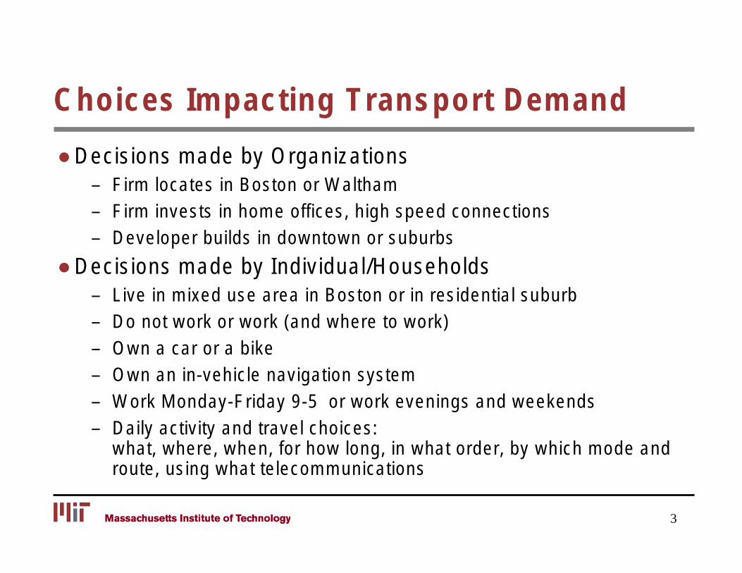
Choices Impacting Transport Demand

● Decisions made by Organizations – Firm locates in Boston or Waltham – Firm invests in home offices, high speed connections – Developer builds in downtown or suburbs

● Decisions made by Individual/Households – Live in mixed use area in Boston or in residential suburb – Do not work or work (and where to work) – Own a car or a bike – Own an in-vehicle navigation system – Work Monday-Friday 9-5 or work evenings and weekends – Daily activity and travel choices:

what, where, when, for how long, in what order, by which mode and route, using what telecommunications

3

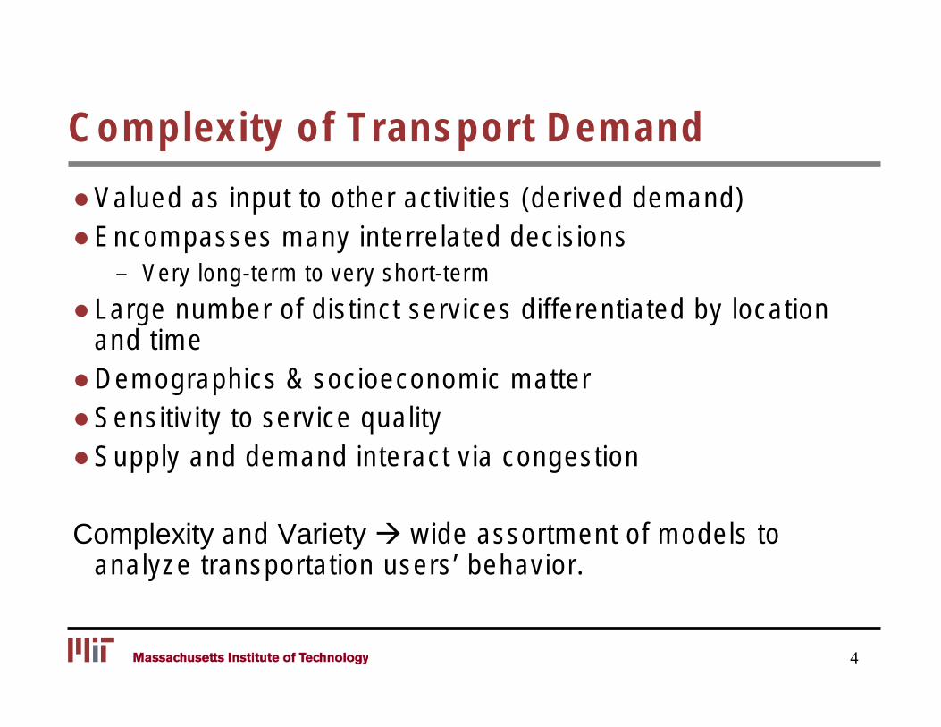
Complexity of Transport Demand

● Valued as input to other activities (derived demand) ● Encompasses many interrelated decisions

– Very long-term to very short-term

● Large number of distinct services differentiated by location and time

● Demographics & socioeconomic matter ● Sensitivity to service quality ● Supply and demand interact via congestion

Complexity and Variety � wide assortment of models to analyze transportation users’ behavior.

4

Mode Share Statistics Transit Shares for Work Trips in Selected U.S. Cities

City Year Transit Mode Share (%)

Boston, MA 1990 10.64 2000 9.03

Chicago, IL 1990 13.66 2000 11.49

New York, NY 1990 26.57 2000 24.90

Houston, TX 1990 3.78 2000 3.28

Phoenix, AZ 1990 2.13 2000 2.02

5

Source: US Census, 1990, 2000

Travel Expenditures ● The average generalized cost (money and time) per person in developed

countries is very stable. %

of

Inco

me

Spen

t on

Tra

vel

5%

10%

15%

20%

100 200 300 400 500 600

Tim

e Sp

ent o

n T

rave

l

14%

~1.1 hrs

Motorization Rate (Cars/1000 Capita)

6

Source: Schäfer A., 1998, “The Global Demand for Motorized Mobility”, Transportation Research A, 32(6): 455-477.

Transport Demand Elasticities

● Elasticity: % change in demand resulting from 1% change in an attribute

● Derived from demand models:

Price In-vehicle time

Work Trips (San Francisco) Auto Bus Rail -0.47 -0.58 -0.86 -0.22 -0.60 -0.60

Price Travel time

Vacation Trips (U.S.) Auto Bus Rail Air -0.45 -0.69 -1.20 -0.38 -0.39 -2.11 -1.58 -0.43

Source: Schäfer A., 1998, “The Global Demand for Motorized Mobility”, Transportation Research A, 32(6): 455-477.

7

Value of Time

● The monetary value of a unit of time for a user.

Work Trips (San Francisco) Auto Bus In-vehicle time 140 76 Percentage of Walk access time 273 after tax wage Transfer wait time 195

Vacation Trips (U.S.) Auto Bus Rail Air Percentage of Total travel time 6 79-87 54-69 149 pretax wage

Freight Rail Truck Percentage of shipment Total transit time 6-21 8-18 value per day

Source: Jose Gómez-Ibañez, William B. Tye, and Clifford Winston, editors, Essays in Transportation Economics and Policy,

8

page 42. Brookings Institution Press, Washington D.C., 1999.

Role of Demand Models

● Forecasts, parameter estimates, elasticities, values of time, and consumer surplus measures obtained from demand models are used to improve understanding of the ramifications of alternative investment and policy decisions.

● Many uncertainties affect transport demand and the models are about to do the impossible

9

Role of Demand Models: Examples

● From Previous Lecture:

– High Speed Rail: Works in Japan/Europe, how about in US?

– Traffic Jams: Build more, manage better, or encourage transit use?

– Truck Traffic: evaluate tradeoffs of environmental protection.

10

Part Two: Overview of Consumer Theory

Outline

● Basic concepts

– Preferences

– Utility

– Choice

● Additional details important to transportation

● Relaxation of assumptions

● Appendix: Dual concepts in demand analysis

11

Preferences

● The consumer is faced with a set of possible consumption bundles

– Consumption bundle: a vector of quantities of different products and services X = {x1,…,xi,…,xm}

– A bundle is an array of consumption amounts of different goods

● Preferences: ordering of the bundles – X fY: Bundle X is preferred to Y

– Behavior: choose the most preferred consumption bundle

– Transitivity, Completeness, and Continuity

12

The Utility Function

● A function that represents the consumer’s preferences ordering X fY ⇔ U(X)>U(Y)

– Utility function is not unique

• U(x1, x2) = ax1 + bx2

• U(x1, x2) = x1ax2

b

– Unaffected by order-preserving transformation

• 10× U(x1, x2) +10 ?

• exp(U(x1, x2)) ?

• (U(x1, x2))2 ?

13

Indifference Curves

● Constant utility curve

● The consumer is indifferent among different bundles on the same curve

x2

u1

u2

u3

Indifference curves

x1

14

Marginal Utility and Trade-offs

● Marginal utility ( ) i

i

U X MU x ∂= ∂

U (x1, x2 ) = 4x1 + 2x2 U (x1, x2 ) = x10.5 x2

0.5

MU 1 = 4 MU 1 = 0.5 x1 −0.5 x2

0.5

● Marginal rate of substitution (MRS)

15

11

2

2

( )

( )

U X MU x

MRS U X MU

x

∂ ∂ = = ∂ ∂

4 2MRS = 2

1

xMRS x =

Consumer Behavior

● Utility (preference) maximization

● Bounded by the available income

max U ( X ) m

s t . . PX ≤ I ( p x ≤ I )∑ i i i=1

X feasible (e.g. non − negativity)

– P - vector of prices P = {p1, …, pi, …, pm}

– I – income

● When considering two goods, the constraint would be:

p1x1 + p2x2 ≤ I

16

Geometry of the Consumer’s Problem

I / p2

Income constraint

x1

x2

u1

u2

u3

Indifference curves

x1 *

x2 *

Slope I / p1

= -p1 / p2

17

Revealed Preferences

● A chosen bundle is revealed preferred to all other feasible bundles:

X (P0 , I 0 ) - the demanded bundle at Point 0

X (P0 , I 0 ) f X (P1, I 1) if P0 X (P0 , I 0 ) ≥ P0 X (P1, I 1)

x2

X(P0, I0)

X(P1, I1) Income

line

x1

18

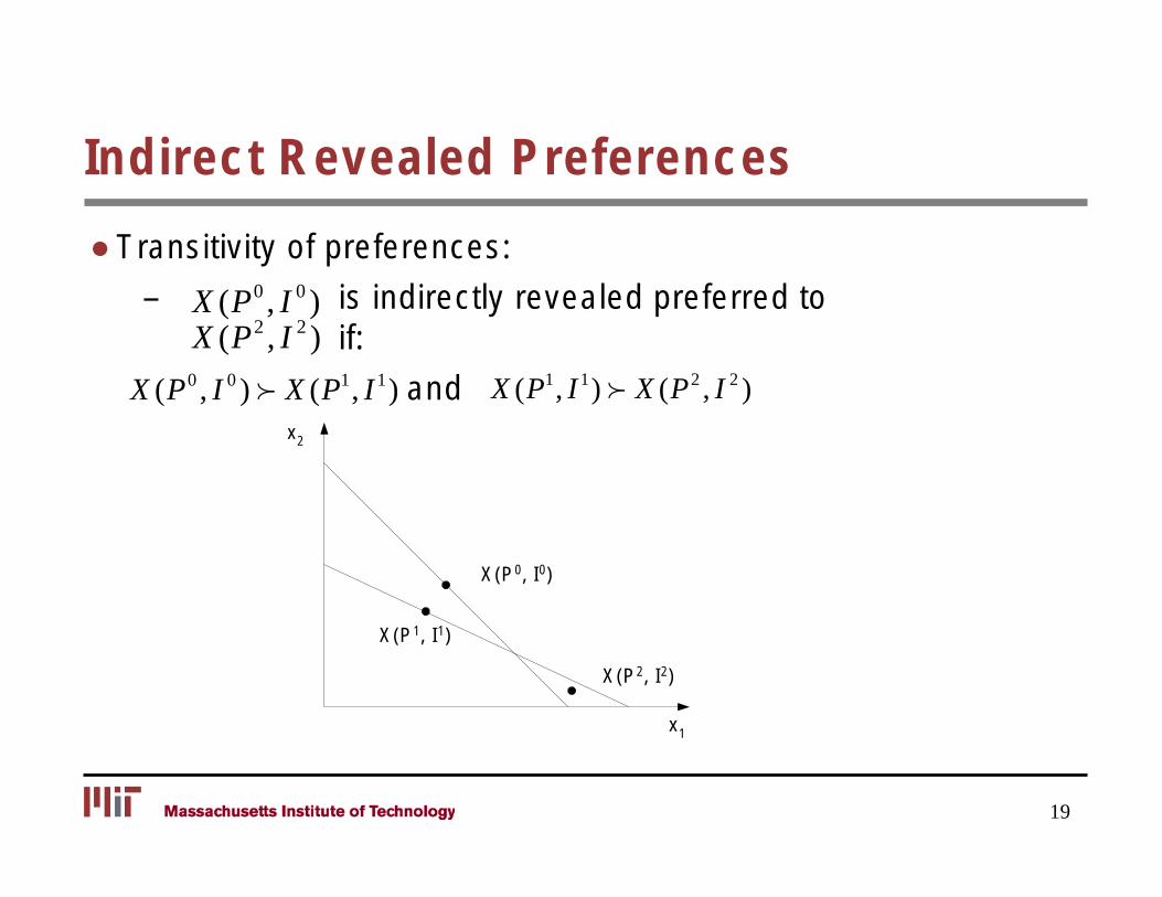
Indirect Revealed Preferences

● Transitivity of preferences:

– X (P0 , I 0 ) is indirectly revealed preferred to X (P2 , I 2 ) if:

X (P0 , I 0 ) f X (P1, I 1) and X (P1, I 1) f X (P2 , I 2 ) x2

X(P0, I0)

X(P1, I1)

X(P2, I2)

x1

19

Optimal Consumption

● The consumer’s problem max U (X ) s.t. PX ≤ I

● Assuming U(X) increases with XPX = I

● The Lagrangean

L(X ,λ) = U (X ) + λ(I − PX )λ: Lagrange multiplier of budget constraint

20

Optimal Consumption

● Optimality conditions:

∂L = ∂U (X *) − λp = 0 ∀i = 1,..., m ∂xi ∂xi

i

*∂U (X )⇒ = λp ∀i

∂xi i

)

* ● Dividing conditions: ∂U (X )

∂U (X

∂xi = p

pi ∀i ≠ j*

∂x j j42431

MRS

21

Example: Cobb-Douglas Utility

● The consumer’s problem: a bmax U ( X ) = x x1 2

s t . . p x + p x ≤ I1 1 2 2

● The Lagrangean: L(X ,λ) = x1 a x2

b + λ(I − p1x1 − p2 x2 )

● Optimal solution: *

2∂L a−1 bx1 = a p

*= ax 1* x2

* − λp1 = 0 x b p∂x1 2 1

∂L * * x * = a I = bx 1

ax2

b−1 − λp2 = 0 1 a + b p∂x2

1

∂L * * x * = b I

∂λ= I − p1x1 − p2 x2 = 0 2 a + b p2

22

Review

Basic concepts – Preferences – Utility functions U(X) – Optimal consumption max U(X) s.t. PX ≤ I – Demand functions X* = X(P,I)

Next… ● Indirect utility ● Complements and Substitutes ● Elasticity ● Consumer surplus

23

Indirect Utility Function

● Recall

X* - the demanded bundle

X(P, I) - the consumer’s demand function

● Indirect utility function – The maximum utility achievable at given prices and budget:

( , ) = max U ( X )V P I

s t . . PX = I

– Substitute the solution X(P, I) back into the utility function to obtain:

maximum utility = V(P, I) = U(X(P, I))

24

Example: Cobb-Douglas Utilitya b

● Recall our earlier problem: max U ( X ) = x1 x2

s t . . p x + p x ≤ I1 1 2 2

* a I * b I x2 =

a + b p1 a + b p2

● We found: x1 =

b aI a + b b

a● So V(p,I) = … =

a b b a b+ +p p a1 2

● What is ∂V ( p, I ) ? ∂I

25

Complements and Substitutes

● Gross substitutes

● Gross complements

∂x j (P, I ) > 0

∂pi

∂x j (P, I ) < 0

∂pi

26

Demand Elasticity

● Percent change in demand resulting from 1% change in an attribute.

% change in X * ΔX * / X *

e.g. price-elasticity = % change in P ΔP / P

– Own elasticity ε px

i

i = xi (

p

Pi

, I )

∂xi

∂ (

p

P

i

, I )

– Cross elasticity ε px j = pi

∂x j (P, I ) i x j (P, I ) ∂pi

27

Consumer Surplus (or Welfare)

● Consumer surplus – difference between the total value consumers receive

from the consumption of a good and the amount paid Price of good 1

Consumer surplus at p11

p11

p10 (p1,I)

Quantity

x1

Loss of surplus when price

28

increases from p1 0 to p1

1

Consumer Surplus

● Consumer surplus is key for evaluating public policy decisions:

– Building transportation infrastructure

– Changing regulations (e.g., emissions)

– Determining fare and service structures

29

Review

● Basic concepts – Preference, Utility, Rationality

● Other useful details – Indirect utility

– Complements and Substitutes

– Elasticity

– Consumer Surplus

Next… Discussion of assumptions

30

Assumptions

● Impact of consumption of one good on utility of another good? ● Income is the only constraint ● Utility is a function of quantities

(a good is a good) ● Demand curves are for an individual ● Behavior is deterministic ● Goods are infinitely divisible (continuous)

31

Separable Utility

● The consumption of one good does not affect the utility received from some other good

m

( ) U (Xi )U X = ∑ i i=1

● Separability into groups of goods

( U U 1 kU X ) = ( (X g1),..., U (X gk )) X gk

- group k of goods

● Allows allocating budget in 2 stages: – Between groups – Within a group

32

Attributes of Goods

Classic: Only quantities matter.

Quantities � Attributes ● The consumer receives utility from attributes of goods

rather then the goods themselves ● Example: (dis)utility of an auto trip depends on travel

time, cost, comfort etc. U = ( ) U AA = A X ( )

– X – Goods – A – Attributes – U – Utility

33

“Household Production” Model

● Consumers purchase goods in order to “produce” utility from them, depending on their attributes

● Classic example: Households purchase food in order to obtain calories and vitamins (could also include enjoyment of taste), which then produce “utility”

34

Utility of a Transportation Mode

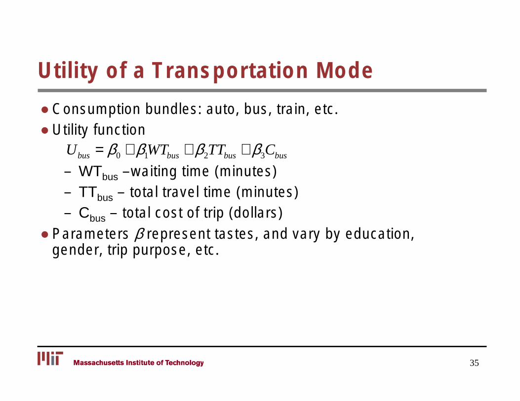
● Consumption bundles: auto, bus, train, etc. ● Utility function

Ubus = β0 + β1WT bus + β2TT bus + β3Cbus

– WTbus –waiting time (minutes) – TTbus – total travel time (minutes) – Cbus – total cost of trip (dollars)

● Parameters β represent tastes, and vary by education, gender, trip purpose, etc.

35

Time Budgets and Value of Time

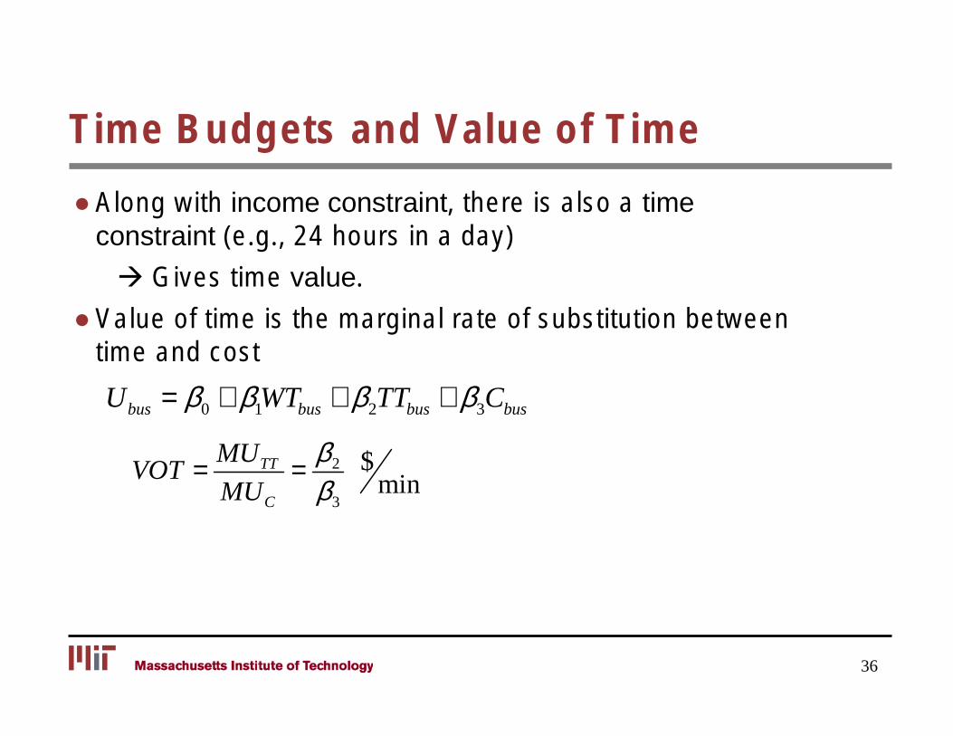
● Along with income constraint, there is also a time constraint (e.g., 24 hours in a day)

� Gives time value.

● Value of time is the marginal rate of substitution between time and cost

Ubus = β0 + β1WT bus + β2TT bus + β3Cbus

VOT = MU TT = β2 $ MU C β3

min

36

Aggregate Consumer Demand

● Aggregate demand is the sum of demands of all consumers

N

X (P, I1,..., IN ) = ∑ X n (P, In ) n=1

– n – An individual consumer – N - # of consumers

● Is this viable? Are individuals sufficiently similar to simply “add up”?

37

Heterogeneity

● Mobility rates, São Paulo, 1987:

Family income Share in population

Mobility rate (all trips)

Mobility rate (motorized trips)

<240 20.8% 1.51 0.59

240-480 28.1% 1.85 0.87

480-900 26.0% 2.22 1.24

900-1800 17.2% 2.53 1.65

>1800 7.9% 3.02 2.28

38

Source: Vasconcellos, 1997, “The demand for cars in developing countries”, Transportation Research A, 31(A): 245-258.

Introducing Uncertainty

● Random utility model

Ui = V(attributes of i; parameters) + epsiloni

● Decision maker deterministic, but analyst imperfect due to:

– Unobserved attributes

– Unobserved taste variations

– Measurement errors

– Use of proxy variables

39

Continuous vs. Discrete Goods

Indifference curves u3

u2 u1

x1

● Continuous goods

● Discrete goods

x2

a u to

b us

40

Summary

● Basic concepts – Preference, Utility, Rationality

● Other useful details – Indirect utility – Complements and Substitutes – Elasticity, Consumer Surplus

● Relaxing the assumptions and working towards practical, empirical models

Next Lecture… Discrete Choice Analysis

41

Appendix

Dual concepts in demand analysis

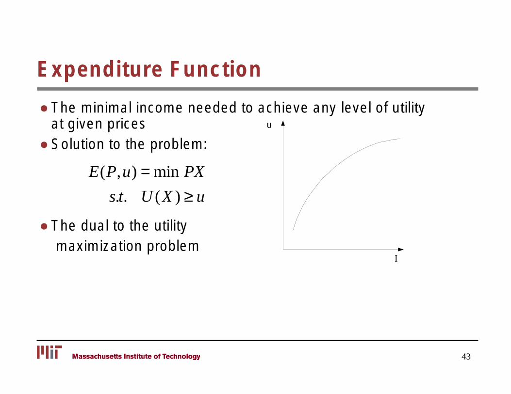
Expenditure Function

● at given prices u

● Solution to the problem:

( , ) = min E P u PX

s t . . ( ) ≥ uU X

● The dual to the utility maximization problem

I

The minimal income needed to achieve any level of utility

43

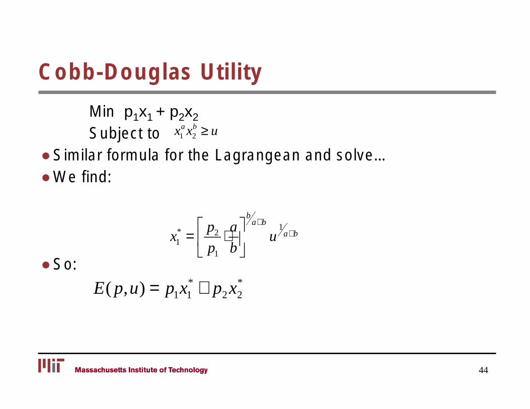
Cobb-Douglas Utility

Min p1x1 + p2x2 x x ≥ u1 2Subject to

a b

● Similar formula for the Lagrangean and solve… ● We find:

b

p a a+b 1

a+bx1* = 2 ⋅ u

p1 b ● So:

E( p,u) = p1x1* + p2 x2

*

44

Consumer Surplus

● Directly related to the expenditure function ● Let E1 = ( 1

1, p2 ,..., pm , 0E p u )and E0 = ( 1

0 , p2 ,..., pm , 0E p u )

● Change in consumer surplus = E0 – E1

45

*

Compensated Demand Function

● The expenditure problem solution:

( , ) = min E P u PX ⇒ X (P u , ) = ( , )H P u

s t . . ( ) ≥ uU X

● H(P,u) is the compensated demand function

● Shows the demand for a good as a function of prices assuming utility is held constant.

● Substituting back into the objective function:

E(P,u) = ∑ pi xi (P,u) = PX (P,u) i

46

Relations Among Demand Concepts

Primal Dual

Max. U(X) s.t. PX =I

Indirect utility function

U*=V(P,I)

Min. E(X) s.t. U(X)=u

Expenditure function

E*=E(P,u)

Demand function

X*=X(P,I)

Demand function

X*=H(P,u)

Inverse

47

MIT OpenCourseWare http://ocw.mit.edu

1.201J / 11.545J / ESD.210J Transportation Systems Analysis: Demand and Economics Fall 2008

For information about citing these materials or our Terms of Use, visit: http://ocw.mit.edu/terms.