Overview of Bohmian Mechanics

Xavier Oriolsa and Jordi Mompartb∗aDepartament d’Enginyeria Electronica, Universitat Autonoma de Barcelona, 08193, Bellaterra, SPAIN

bDepartament de Fısica, Universitat Autonoma de Barcelona, 08193 Bellaterra, SPAIN

This chapter provides a fully comprehensive overview of the Bohmian formulation of quantumphenomena. It starts with a historical review of the difficulties found by Louis de Broglie, DavidBohm and John Bell to convince the scientific community about the validity and utility of Bohmianmechanics. Then, a formal explanation of Bohmian mechanics for non-relativistic single-particlequantum systems is presented. The generalization to many-particle systems, where correlations playan important role, is also explained. After that, the measurement process in Bohmian mechanicsis discussed. It is emphasized that Bohmian mechanics exactly reproduces the mean value andtemporal and spatial correlations obtained from the standard, i.e., ‘orthodox’, formulation. Theontological characteristics of the Bohmian theory provide a description of measurements in a naturalway, without the need of introducing stochastic operators for the wavefunction collapse. Severalsolved problems are presented at the end of the chapter giving additional mathematical supportto some particular issues. A detailed description of computational algorithms to obtain Bohmiantrajectories from the numerical solution of the Schrodinger or the Hamilton–Jacobi equations arepresented in an appendix. The motivation of this chapter is twofold. First, as a didactic introductionof the Bohmian formalism which is used in the subsequent chapters. Second, as a self-containedsummary for any newcomer interested in using Bohmian mechanics in their daily research activity.

∗ E-mail: xavier.oriols@uab.cat; jordi.mompart@uab.cat

arX

iv:1

206.

1084

v3 [

quan

t-ph

] 3

May

201

9

2

This paper entitled “Overview of Bohmian Mechanics” includes the two

prefaces, the introduction and the first chapter of the second edition of

the book “Applied Bohmian Mechanics: From Nanoscale Systems to

Cosmology”. The whole book, with nine additional chapters, has been

published by Pan Stanford editorial and it can be ordered as indicated

below.

This paper has to be cited as:

X. Oriols and J. Mompart “Overview of Bohmian Mechanics”; Chapter 1 of the

book “Applied Bohmian Mechanics: From Nanoscale Systems to Cosmology”.

Editorial Pan Stanford Publishing Pte. Ltd (Second edition, 2019).

Print ISBN: 9789814800105

How to Order: You can place an order from any good bookstores or email us at sales@panstanford.com for more information.

http://www.panstanford.com/

3

CONTENTS

I. Preface first edition 4New cutting edge ideas come from outside of the main stream 4

II. Preface second edition: 6Quantum engineering: a giant with feet of clay 6

III. Introduction 7III.1. What is a quantum theory 8III.2. How Bohmian mechanics helps 9III.3. On the name Bohmian mechanics 10III.4. On the book contents 11

IV. Historical Development of Bohmian Mechanics 13IV.1. Particles and waves 13IV.2. Origins of the quantum theory 14IV.3. “Wave or particle?” vs. “wave and particle” 15IV.4. Louis de Broglie and the fifth Solvay Conference 17IV.5. Albert Einstein and locality 17IV.6. David Bohm and why the “impossibility proofs” were wrong? 18IV.7. John Bell and nonlocality 20IV.8. Quantum hydrodynamics 21IV.9. Is Bohmian mechanics a useful theory? 21

V. Bohmian Mechanics for a Single Particle 22V.1. Preliminary discussions 22V.2. Creating a wave equation for classical mechanics 22

V.2.1. Newton’s second law 22V.2.2. Hamilton’s principle 23V.2.3. Lagrange’s equation 24V.2.4. Equation for an (infinite) ensemble of trajectories 24V.2.5. Classical Hamilton–Jacobi equation 26V.2.6. Local continuity equation for an (infinite) ensemble of classical particles 26V.2.7. Classical wave equation 26

V.3. Trajectories for quantum systems 27V.3.1. Schrodinger equation 27V.3.2. Local conservation law for an (infinite) ensemble of quantum trajectories 27V.3.3. Velocity of Bohmian particles 28V.3.4. Quantum Hamilton–Jacobi equation 28V.3.5. A quantum Newton-like equation 29

V.4. Similarities and differences between classical and quantum mechanics 30V.5. Feynman paths 32V.6. Basic postulates for a single-particle 33

VI. Bohmian Mechanics for Many-Particle Systems 34VI.1. Preliminary discussions: The many body problem 34VI.2. Many-particle quantum trajectories 35

VI.2.1. Many-particle continuity equation 36VI.2.2. Many-particle quantum Hamilton–Jacobi equation 36

VI.3. Factorizability, entanglement, and correlations 37VI.4. Spin and identical particles 38

VI.4.1. Single-particle with s = 1/2 38VI.4.2. Many-particle system with s = 1/2 particles 40

VI.5. Basic postulates for many-particle systems 41VI.6. The conditional wave function: many-particle Bohmian trajectories without the many-particle wave

function 42VI.6.1. Single-particle pseudo-Schrodinger equation for many-particle systems 43

4

VI.6.2. Example: Application in factorizable many-particle systems 45VI.6.3. Example: Application in interacting many-particle systems without exchange interaction 45VI.6.4. Example: Application in interacting many-particle systems with exchange interaction 47

VII. Bohmian Explanation of the Measurement Process 49VII.1. The measurement problem 49

VII.1.1. The orthodox measurement process 51VII.1.2. The Bohmian measurement process 52

VII.2. Theory of the Bohmian measurement process 53VII.2.1. Example: Bohmian measurement of the momentum 56VII.2.2. Example: Sequential Bohmian measurement of the transmitted and reflected particles 56

VII.3. The evaluation of a mean value in terms of Hermitian operators 60VII.3.1. Why Hermitian operators in Bohmian mechanics? 60VII.3.2. Mean value from the list of outcomes and their probabilities 60VII.3.3. Mean value from the wave function and the operators 61VII.3.4. Mean value from Bohmian mechanics in the position representation 61VII.3.5. Mean value from Bohmian trajectories 61VII.3.6. On the meaning of local Bohmian operators AB(x ) 63

VIII. Concluding Remarks 63

Acknowledgments 64

IX. Problems and solutions 64

X. Appendix: Numerical Algorithms for the Computation of Bohmian Mechanics 72X.1. Analytical computation of Bohmian trajectories 73

X.1.1. Time-dependent Schrodinger equation for a 1D space (TDSE1D-BT) with an explicitmethod 74

X.1.2. Time-independent Schrodinger equation for a 1D space (TISE1D) with an implicit (matrixinversion) method 75

X.1.3. Time-independent Schrodinger equation for a 1D space (TISE1D) with an explicit method 77X.2. Synthetic computation of Bohmian trajectories 79

X.2.1. Time-dependent quantum Hamilton–Jacobi equations (TDQHJE1D) with an implicit(Newton-like fixed Eulerian mesh) method 80

X.2.2. Time-dependent quantum Hamilton–Jacobi equations (TDQHJE1D) with an explicit(Lagrangian mesh) method 81

X.3. More elaborated algorithms 83

References 83

I. PREFACE FIRST EDITION

New cutting edge ideas come from outside of the main stream

Most of our collective activities are regulated by other people who decide whether they are well done or not. Onehas to learn some arbitrary symbols to write understandable messages, or to read those from others. Human rulesover collective activities govern the evolution of our culture. On the contrary, natural systems, from atoms to galaxies,evolve independently of the human rules. Men cannot modify physical laws. We can only try to understand them.Nature itself judges, through experiments, whether a plausible explanation for some natural phenomena is correct ornot. Nevertheless, in forefront research where the unknowns start to become understandable, the new knowledge isstill unstable, somehow immature. It is supported by few experimental evidences or the evidences are still subjectedto different interpretations. Certainly, novel research grows up closely tied to the economical, sociological or historicalcircumstances of the involved researchers. A period of time is needed in order to distil new knowledge, separatingpure scientific arguments from cultural influences.

The past and the present status of Bohmian mechanics cannot be understood without these cultural considerations.The Bohmian formalism was proposed by Louis de Broglie even before the standard, that is Copenhagen, explanationof quantum phenomena was established. Bohmian mechanics provides an explanation of quantum phenomena in terms

5

of particles guided by waves. One object cannot be a wave and a particle simultaneously, but two can. Specially, ifone of the objects is a wave and the other is a particle. Unfortunately, Louis de Broglie, himself, abandoned theseideas. Later, in the fifties, David Bohm clarified the meaning and applications of this original explanation of quantumphenomena. Bohmian mechanics agrees with all non-relativistic quantum experiments done up to now. However,it remains almost ignored by most of the scientific community. In our opinion, there are no scientific arguments tosupport its marginal status, but only cultural reasons. One of the motivations for writing this book is helping in thematuring process that Bohmian mechanics still needs.

Certainly, the distilling process of Bohmian mechanics is being quite slow. Anyone interested enough to walk thiscausal road of quantum mechanics can be easily confused by many misleading signposts that have been raised in thescientific literature, not only by its detractors, but unfortunately very often also by some of its advocates. Followingopinions from other reputed physicists (we are easily persuaded by those scientists with authority) is far from beinga proper scientific strategy.

In any case, since the mathematical structure of Bohmian mechanics is quite simple, it can be easily learned byanyone with only a basic knowledge of classical and quantum mechanics who makes the necessary effort to buildhis own scientific opinion based on logical deductions, free from cultural influences. The introductory chapter of thisbook, including a thorough list of exercises and easily programmable codes, provides a reasonable and objective sourceof information in order to achieve this later goal, even for undergraduate students.

Curiously, the fact that Bohmian mechanics is ignored and remains mainly unexplored is an attractive feature forsome adventurous scientists. They know that very often new cutting edge ideas come from outside of the main streamand find in Bohmian mechanics a useful tool in their research activity. On the one hand, it provides an explanationof quantum mechanics, in terms of trajectories, that results to be very useful in explaining the dynamics of quantumsystems, being thus also a source of inspiration to look for novel quantum phenomena. On the other hand, sinceit provides an alternative mathematical formulation, Bohmian mechanics offers new computational tools to explorephysical scenarios that presently are computationally inaccessible, such as many particle solutions of the Schrodingerequation. In addition, Bohmian mechanics sheds light on the limits and extensions of our present understanding ofquantum mechanics towards other paradigms such as relativity or cosmology, where the internal structure of Bohmianmechanics in terms of well-defined trajectories is very attractive. With all these previous motivations in mind, thisbook provides nine chapters (apart from the introduction in the first chapter) with practical examples showing howBohmian mechanics helps us in our daily research activity.

Obviously, there are other books focused on Bohmian mechanics. However, many of them are devoted to thefoundations of quantum mechanics emphasizing the difficulties or limitations of the Copenhagen interpretation forproviding an ontological description of our world. On the contrary, this book is not focus on the foundations ofquantum mechanics, but on the discussion about the practical application of the ideas of de Broglie and Bohm tounderstand and compute the quantum world. Several examples of such practical applications written by leadingexperts in different fields, with an extensive updated bibliography, are provided here. The book, in general, isaddressed to students in physics, chemistry, electrical engineering, applied mathematics, nanotechnology, as well as toboth theoretical and experimental researchers who seek new computational and interpretative tools for their everydayresearch activity. We hope that the newcomers to this causal explanation of quantum mechanics will use Bohmianmechanics in their research activity so that Bohmian mechanics will become more and more popular for the broadscientific community. If so, we expect that, in the near future, Bohmian mechanics will be taught regularly at theUniversities, not as the unique and revolutionary way of understanding quantum phenomena, but as an additionaland useful interpretation of all quantum phenomena in terms of quantum trajectories. In fact, Bohmian mechanicshas the ability of removing most of the mysteries of the Copenhagen interpretations and, somehow, simplifying (ordemystifying) quantum mechanics. We will be very glad if this book can contribute to shorten the time needed toachieve all these goals.

Finally, we want to acknowledge many different people that has allowed us to embark into and successfully finishthis book project. First of all, Alfonso Alarcon and Albert Benseny who became involved in the book project fromthe very beginning, as two additional editors. We also want to thank the rest of the authors of the book for acceptingour invitation to participate in this project and writing their chapters according to the general spirit of the book. Dueto page limitations, only nine examples of practical applications of Bohmian mechanics in forefront research activityare presented in this book. Therefore, we want to apologize to many other researchers who could have certainly beenalso included in the book. We also want to express our gratitude to Pan Stanford Publishing for accepting our bookproject and for their kind attention during the publishing process.

6

II. PREFACE SECOND EDITION:

Quantum engineering: a giant with feet of clay

More than five years after the first edition of our book on applied Bohmian mechanics, our original motivations forwriting it are still very present. Certainly, today, a lot of publicity about the abilities of the Bohmian theory is stillneeded among the scientific community. In fact, over these last few years, many research programs have been devotedto the so-called quantum engineering with the goal of developing new materials, new sensors, or new computingstrategies based on pure quantum phenomena. Thus, this book can be understood as a promotional presentationon how the Bohmian theory, among others, can help in the design and development of such applications. However,Bohmian mechanics is not a mere computational tool in terms of quantum trajectories, but a complete and ontologicaltheory that provides a consistent explanation on how Nature works. In this regard, this book can also be seen as auseful exercise to sincerely question our present understanding of the physical laws that govern the quantum world.After a bit of reflection on this point, many of us will probably conclude that our knowledge about the fundamentalsof the quantum world are much more immature and imprecise than what we previously thought. In this sense, wewant this book to be a warning on the the risks of constructing the new and exciting discipline of quantum engineeringas a giant with feet of clay.

The beginning of the 20th century saw the first quantum revolution where novel and original theories were developedto understand unexpected non-classical phenomena. What determines the structure of the periodic table? Why aresome materials metals and some dielectrics, while others behave like semiconductors? Nowadays, having establishedanswers to these basic questions, a second quantum revolution is starting to take place, focusing on actively capitalizingon our quantum knowledge to alter the face of the physical world, developing a myriad of new quantum technologies.The difference between these two quantum revolutions is just the difference between science and engineering. The firstrevolution tried to properly understand our physical surroundings, the natural objects around us, while the second oneintends to manipulate these surroundings to our own benefit. This is the typical evolution of most scientific disciplines.When scientific knowledge is mature enough, and the necessary technological means are available, engineers can usethis knowledge for practical applications.

It is a common belief in our society that quantum theory, after more than a century, is ready to take a leaptowards the engineering field. We have certainly outstanding technological means to manipulate quantum systems,even individual atoms, at the nanometer and femtosecond scales. Therefore, many national or international researchorganizations are focusing their programs towards the effective development of quantum technologies, trying to ensurethat money spent on science has a direct impact on our society and its challenges for a better life. This is indeed alegitimate and compelling goal. However, is the quantum theory mature enough to blindly jump from science towardsengineering? The pressure from society (in terms of research programs, grants, citing indices, etc.) is so effective thatit forces most of the scientists to forget about the maturity of the quantum theory and just focus on (what reallymatters) the fast development of practical applications in the new and exciting field of quantum engineering.

We argue that the development of quantum engineering cannot be done at the price of forgetting the need for adeeper understanding of the physical laws governing the quantum world. One of the forgotten discussions by the newgeneration of quantum engineers is the measurement problem, which remains inside the backbone of the quantumtheory. The measurement problem is manifested in the orthodox theory by its failure in explaining which physicalinteractions among particles constitute a measurement and which do not. In fact, there are many more examplesof the immaturity of our quantum knowledge. Our inability to properly describe many-body systems due to theirexponential complexity (the so-called many-body problem) makes that most of our understanding is based on apuerile single-particle description. We do not have a clear physical picture on the quantum-to-classical transition.What makes a quantum system to behave classically in some circumstances? The fact that there are several quantumtheories which are empirically equivalent but radically different at the ontological level is a clear evidence of our badunderstanding. The Copenhagen theory is the most extensively investigated and presently the one with more supportamong the scientific community. Others include spontaneous collapse theories or the many-worlds theory. The onestudied in this book, Bohmian mechanics, provides a description of quantum phenomena by particles choreographedby the wave function. In general, neither of these theories is more mature than the orthodox one, but they remove theneed of an observer, which relaxes some of the difficulties to understand the measurement at a quantum level. Some ofthese alternative theories are not free of problems, including the quantum-to-classical transition and the many-bodyproblem, while others still need to be dealt with. We do not mean to imply that these alternative theories are better(how does one quantify better here?), but that there is still a lot of work needed to certify that our comprehension ofthe quantum world is unproblematic.

Let us try to exemplify the risks of developing quantum engineering alone without worrying on its fundamentals.In the orthodox theory, every time we make a measurement a random process occurs. But, as we do not really knowwhat makes a physical interaction to be a measurement, we really do not know the origin of such randomness. In

7

the Bohmian theory, for example, this randomness comes from an uncertainty in the initial position of the particles.With further efforts to clarify the quantum theories, we can perhaps achieve a better understanding of the origin ofquantum randomness and then, the exciting new building of application developed along the new discipline of quantumcryptography, based on the unavoidable presence of such intrinsic quantum randomness, will simple melt as a giantwith feet of clay. The reader can argue that there are a lot of scientific works supporting the actual status of quantumcryptography. Perhaps this particular warning is completely unfounded and quantum cryptography will certainlyremain as robust as we know today. But, perhaps not. It is enlightening to remember here the theorem that Johnvon Neumann stated in 1932 about the impossibility of explaining quantum mechanics with hidden variables (suchas quantum trajectories). This theorem remained an unquestionable truth, and part of the essence of the quantumworld, until David Bohm (with an explanation of quantum phenomena in terms of waves and particles) showed thatthe theorem was wrong (as its own preliminary assumptions precludes the existence of Bohmian trajectories). Thecurious spectacle is not that John von Neumann (an outstanding scientist in many disciplines) made a mistake in atheorem, but that the community (with the exception of Grete Hermann in 1935 that was totally ignored) blindlyaccepted the theorem for almost half a century.

There are many more examples which certify that our understanding of the quantum world is still immature. Thewave function, the basic element in most theories, can be prepared for instance by forcing the quantum system into itsground state, but it cannot be directly measured in a single experiment. The wave function can be measured througha weak protocol, but also Bohmian velocities can be measured though such protocol. We do not even know what isreally the wave function at the most fundamental level: a law? a field? a probability transporter?

In summary, the quantum world is so complicated that one century has not been enough for the scientific communityto clearly elaborate an unproblematic description of the laws of quantum mechanics. We are not arguing here thatresearch on quantum engineering needs to stop. Just the contrary. The development of the quantum engineering andthe research on the foundations of the quantum theory have to evolve intimately connected to benefice from eachother in achieving better practical applications and a deeper understanding of the quantum world. Otherwise, wewill build a giant with feet of clay. We hope that the present book can be viewed as a modest contribution in bothdirections.

III. INTRODUCTION

The beginning of the twentieth century brought surprising non-classical phenomena. Max Planck’s explanation ofthe black body radiation [1], the work of Albert Einstein on the photoelectric effect [2] and the Niels Bohr’s model toaccount for the electron orbits around the nuclei [3–5] established what is now known as the old quantum theory. Todescribe and explain these effects, phenomenological models and theories were first developed, without rigorous justi-fication. In order to provide a complete explanation for the underlying physics of such new non-classical phenomena,physicists were forced to abandon classical mechanics to develop novel, abstract and imaginative formalisms.

In 1924, Louis de Broglie suggested in his doctoral thesis that matter, apart from its intrinsic particle-like behavior,could exhibit also a wave-like one [6]. Three years later he proposed an interpretation of quantum phenomena basedon non-classical trajectories guided by a wave field [7]. This was the origin of the pilot-wave formulation of quantummechanics that we will refer as Bohmian mechanics to account for the following work of David Bohm [8, 9]. In theBohm formulation, an individual quantum system is formed by a point particle and a guiding wave. Contemporanely,Max Born and Werner Heisenberg, in the course of their collaboration in Copenhagen with Niels Bohr, provided anoriginal formulation of quantum mechanics without the need of trajectories [10, 11]. This was the origin of the so-calledCopenhagen interpretation of quantum phenomena and, since it is the most accepted formulation, it is basically theonly one explained at most universities. Thus, it is also known as the orthodox formulation of quantum mechanics.In the Copenhagen interpretation, an individual quantum system exhibits its wave or its particle nature dependingon the experimental arrangement.

The present status of Bohmian mechanics among the scientific community is quite marginal (the quantum chemistrycommunity is an encouraging exception). Most researchers do not know about it or believe that is not fully-correct.There are others that know that quantum phenomena can be interpreted in terms of trajectories, but they think thatthis formalism cannot be useful in their daily research activity. Finally, there are few researchers, the authors of thisbook among them, who think that Bohmian mechanics is a useful tool to make progress in front-line research fieldsinvolving quantum phenomena.

The main (non-scientific) reason why still many researchers believe that there is something wrong with Bohmianmechanics can be illustrated with Hans Christian Andersen’s tale The Emperor’s new clothes. Two swindlers promisethe Emperor the finest clothes that, as they tell him, are invisible to anyone who is unfit for their position. TheEmperor cannot see the (non-existing) clothes, but pretends that he can for fear of appearing stupid. The rest of thepeople do the same. Advocates of the Copenhagen interpretation have attempted to produce impossibility proofs in

8

order to demonstrate that Bohmian mechanics is incompatible with quantum phenomena [12]. Most researchers, whoare not aware of the incorrectness of such proofs, might conclude that there is some controversy with the Bohmianformulation of quantum mechanics and they prefer not to support it, for fear of appearing discordant. At the end ofthe tale, during the course of a procession, a small child cries out “the Emperor is naked!”. In the tale of quantummechanics, David Bohm [8, 9] and John Bell [13] were the first to exclaim to the scientific community “Bohmianmechanics is a correct interpretation of quantum phenomena that exactly coincides with the predictions of the orthodoxinterpretation!”.

III.1. What is a quantum theory

Albert Einstein, in the paper entitled “Physics and reality” [14], pointed out the possibility of living in a bizarre worldwithout comprehensible explanations for natural phenomena. He wrote: “The fact that [the world] is comprehensibleis a miracle”. Similarly, Eugene Wigner wrote: “The unreasonable effectiveness of mathematics in the natural science....is a wonderful gift which we neither understand nor deserve” [15]. Both reflections were inspired by the previouswork of the German philosopher Immanuel Kant who wrote the very same idea almost two centuries before: “Theeternal mystery of the world is its comprehensibility.”. Fortunately, it seems that we live in a comprehensible world.

Kant divided scientific knowledge into three categories: appearance, reality and theory. Appearance is the contentof our sensory experience of natural phenomena, which is the empirical outcome of an experiment. Reality is whatlies behind all natural phenomena. A theory is a human model that tries to mirror both appearance and reality. Auseful theory might predict the outcome of an experiment in a laboratory or the observation of a phenomenon inNature. Empiricists believe on experimental outcomes (what Kant called appearance) and refuse to speculate abouta deeper reality. On the other hand, realists believe that good physical theories explain, or at least provide cluesabout, the reality of our comprehensible world. Most researchers are a combination of both stereotypes, with variableproportions.

As all human creations, there are successful and unsuccessful theories. When in 1864 James Clerk Maxwell conjec-tured that light was an electromagnetic vibration, it was believed that all waves had to vibrate in some medium. Themedium in which light presumably travels was named luminiferous ether. During almost a century eminent scientistsbelieved blindly on that concept. Nowadays, the luminiferous ether plays no role at all in modern physical theories[16].The atomicity of matter is an example of a very successful theory. It was introduced by the British chemist JohnDalton in 1808 to explain why some chemical substances need to combine in some fixed ratios. During one centuryit was thought that atoms were a crazy idea. Marcelin Berthelot said “who [has] ever seen a gas molecule or anatom?”, expressing the disdain that many chemists felt for the unseen atoms, which were inaccessible to experiments[16]. Even their defenders saw little hope of ever directly verifying the atomic hypothesis. Nowadays, the fact thateverything is made of atoms is one of the most precious knowledge that we get on how Nature works[17], and theirimages are even routinely seen in the screens of scanning tunneling microscopes [18].

A quantum theory is a human explanation of quantum phenomena. All quantum theories have associated theirown intangible reality. The so-called ontology of the theory. For example, the ontology of the Bohmian theory is verysimple: everything is build by point particles guided (“choreographed”) by waves. The different quantum theoriesavailable today (Copenhagen, Bohmian, many worlds, spontaneous collapse, etc.) are indeed inspired by radicallydifferent realities, but all of them provide the same empirical predictions on quantum phenomena. In Kant’s words,all of them provide the same explanation of the appearance of our world. As we repeatedly stressed, up to know,in spite of many attempts, there is no experimental evidence that can discern between Bohmian and Copenhagenrealities (ontologies).

In fact, for practical applications, even wrong theories can be very useful. Most natural phenomena that affect ourordinary life can be exclusively explained in terms of classical mechanics. However, today, we know that the realitybehind the classical theory is wrong because it does not provide accurate predictions for some natural phenomena,like relativistic (with particles with high velocities) or quantum (atomistic dimensions) experiments. Surprisingly, thefact that the classical theory is a wrong theory does not demerit its extraordinary utility and our confidence on itspredictions within its range of validity1. The same is true for most physical theories at a practical level. Even if wecould demonstrate in the future that either the Copenhagen or the Bohmian theories is wrong (or both), the practicalutility of these theories in their range of validity would not dismiss.

1 We take classical planes expecting that they will follow a deterministic trajectory, e.g., from Barcelona to Paris. However, we knowthat quantum uncertainty precludes us to affirm that there is only one possible trajectory for the fly departing from Barcelona. Evenafter doing our best to fix the initial conditions of the physical degrees of the plane, there is still an unavoidable quantum randomnessimplying that several trajectories are possible. Of course, the differences between trajectories are so small at a macroscopic level thatthe pilot can easily certify that we will arrive to Paris.

9

III.2. How Bohmian mechanics helps

Although there is no experimental evidence against Bohmian mechanics, many researchers believe that Bohmianmechanics is not a useful tool to do research. In the words of Steven Weinberg, in a private exchange of letters withSheldon Goldstein [19]: “In any case, the basic reason for not paying attention to the Bohm approach is not somesort of ideological rigidity, but much simpler — it is just that we are all too busy with our own work to spend time onsomething that doesn’t seem likely to help us make progress with our real problems.”.

The history of science seems to give credit to Weinberg‘s sentence. In spite of the controversies that have alwaysbeen associated with the Copenhagen interpretation since its birth a century ago, its mathematical and computationalmachinery has enabled physicists, chemists and (quantum) engineers to calculate and predict the outcome of a vastnumber of experiments, while the contribution of Bohmian mechanics during the same period is much less significative.The differences are due to the fact that Bohmian mechanics remains mainly unexplored.

Contrarily to Weinberg’s opinion, we believe that Bohmian mechanics can help us make progress with our realproblems. There are, at least, three clear reasons why one could be interested in studying quantum problems withBohmian mechanics:

1. Bohmian explaining : Even when the Copenhagen mathematical machinery is used to compute observableresults, the Bohmian interpretation ofently offers different interpretational tools. We can find descriptions ofelectron dynamics such as “an electron crosses a resonant tunneling barrier and interacts with another electroninside the well”. However, according to the orthodox theory, we can only talk about the properties of anelectron (for example, its position) when we measure it. If we do not measure it, the electron has no property.Thus, an electron crossing a tunneling region is not rigorously supported within orthodox quantum mechanics,but it is within the Bohmian picture. Thus, in contrast to the Copenhagen theory, Bohmian mechanics allowsfor an easy visualization of quantum phenomena in terms of trajectories that has important demystifying orclarifying consequences. In fact, Bohmian mechanics allows for an unambiguous2 description of measured andunmeasured properties of particles (an electron crossing a tunneling barrier is a description of unmeasured prop-erties). Bohmian mechanics provides a single-event description of the experiment, while Copenhagen quantummechanics accounts for its statistical or ensemble explanation. We will present several examples in chapters 2and 3 emphasizing all these points.

2. Bohmian computing : Although the predictions of the Bohmian interpretation reproduce the ones of theorthodox formulation of quantum mechanics, its mathematical formalism is different. In some systems, theBohmian equations might provide better computational tools than the ones obtained from the orthodox ma-chinery, resulting in a reduction of the computational time, an increase in the number of degrees of freedomdirectly simulated, etc. We will see examples of these computational issues in quantum chemistry in chapters 4and 5, as well as in quantum electron transport in Chap. 6.

3. Bohmian thinking : From a more fundamental point of view, alternative formulations of quantum mechanicscan provide alternative routes to look for the limits and possible extensions of the quantum theory. In particular,Chap. 7 presents the route to connect Bohmian mechanics with geometrical optics and beyond opening the wayto apply the powerful computational tools of quantum mechanics to classical optics, and even to electromag-netism. The natural extension of Bohmian mechanics to the relativistic regime and to quantum field theory arepresented in Chap. 8, while Chap. 9 and Chap. 10 discusses its application to cosmology.

The fact that all measurable results of the orthodox quantum mechanics can be exactly reproduced with Bohmianmechanics (and vice versa) is the relevant point that completely justifies why Bohmian mechanics can be used forexplaining or computing different quantum phenomena in physics, chemistry, electrical engineering, applied math-ematics, nanotechnology, etc. In the scientific literature, the Bohmian computing technique to find the trajectories(without directly computing the wavefunction) is also known as a syntectic technique, while the Bohmian explainingtechnique (where the wavefunction is directly computed first) is referred as the analytic technique [20]. Furthermore,the fact that Bohmian mechanics is a theory without observers is an attractive feature for those researchers interestedin thinking about the limits or extensions of the quantum theory.

2 About the ambiguity of the orthodox explanation of quantum mechanics and the unambiguity of Bohmian mechanics, J. Bell wrote[13](page 111): “I will try to interest you in the de Broglie - Bohm version of non-relativistic quantum mechanics. It is, in my opinion, veryinstructive. It is experimentally equivalent to the usual version insofar as the latter is unambiguous.”

10

In order to convince the reader about the practical utility of Bohmian mechanics for explaining , computingor thinking , we will not present elaborated mathematical developments or philosophical discussions, but providepractical examples. Apart from the first chapter, devoted to an overview of Bohmian mechanics, the book is dividedinto nine additional chapters with several examples on the practical application of Bohmian mechanics to differentresearch fields, ranging from atomic systems to cosmology. These examples will clearly show that the previousquotation by Weinberg does not have to be always true.

III.3. On the name Bohmian mechanics

Any possible newcomer to Bohmian mechanics can certainly be quite confused and disoriented by the large listof names and slightly different explanations of the original ideas of de Broglie and Bohm that are present in thescientific literature. Different researchers use different names. Certainly, this is an indication that the theory is stillnot correctly settled down among the scientific community.

In his original works [6, 7], de Broglie used the term pilot-wave theory [21], to emphasize the fact that wave-fieldsguided the motion of point particles. After de Broglie abandoned his theory, Bohm rediscovered it in the seminalpapers entitled “A suggested interpretation of the quantum theory in terms of hidden variables” [8, 9]. The term hiddenvariables3, refering to the positions of the particles, was perhaps pertinent in 1952, in the context of the impossibilityproofs [12]. Nowadays, these words might seem inappropriate because they suggest something metaphysical on thetrajectories4.

To give credit to both de Broglie and Bohm, some researchers refer to their works as the de Broglie–Bohm theory5[24].Some reputed researchers argue that de Broglie and Bohm did not provide the same exact presentation of the theory[21, 25]. While de Broglie presented a first order development of the quantum trajectories (integrated from thevelocity), Bohm himself did a second order (integrated from the acceleration) emphasizing the role of the quantumpotential. The differences between both approaches appear when one considers initial ensembles of trajectories whichare not in quantum equilibrium6. Except for this issue, which will not be addressed in this book, both approachesare identical.

Many researchers prefer to use the name Bohmian mechanics [26]. It is perhaps the most popular name. We knowdirectly from his alive collaborators, Basile Hiley and David Peat [27], that this name irritated David Bohm and he saidabout its own work “it’s Bohmian non-mechanics”. He argued that the ’quantum potential’ is a non-local potentialthat depends on the relative shape of the wavefunction and thus it is completely different from other mechanical (suchas the gravitational or the electrostatic) potentials which decrease with distance. See this particular discussion in thelast chapters of Bohm and Hiley’s book entitled The Undivided Universe: An Ontological Interpretation of QuantumTheory [28]. He preferred the names causal or ontological interpretation of quantum mechanics [24, 28]. The latternames emphasize the foundational aspects of its formulation of quantum mechanics.

Finally, another very common term is quantum hydrodynamics [20] that underlines the fact that Bohmian trajec-tories provide a mathematical relationship between the Schrodinger equation and fluid dynamics. In fact, this nameis more appropriate when one refers to the Madelung theory [29], which is considered as a precursor of Bohm’s work,see Sec. IV.8.

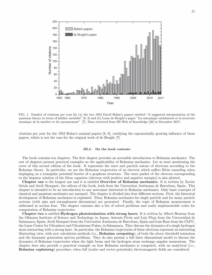
From all these different names, we choose Bohmian mechanics because it is short and clearly specifies what weare referring to. It has the inconvenience of not giving credit to the initial work of Louis de Broglie. Although itmight be argued that Bohm merely reinterpreted the prior work of de Broglie, we think that he was the first person togenuinely understand its significance and implications. As we mentioned, Bohm himself disliked this name. However,as any work of art, the explanation of the quantum phenomena done in the 1952 Bohm’s paper does not completelybelong to the author7, but has become part of our scientific heritage. It has happened many times during the historyof science that the mathematical equation developed by a scientist contains much more physical substance than whathe/she imagined at the beginning. In any case, we understand Bohmian mechanics as a generic name that includesall those works inspired from the original ideas of Bohm and de Broglie. In the figure below, we plot the numbers of

3 Note that the term hidden variables can also refer to other (local and non-local) formulations of quantum mechanics.4 Sometimes it is argued that the name hidden variables is because Bohmian trajectories cannot be measured directly. However, what

is not directly measured in experiments is the (complex) wavefunction amplitude, while the final positions of particles can be directlymeasured, for example, by the imprint they leave on a screen. John S. Bell wrote [13] (page 201): “Absurdly, such theories are knownas ’hidden variable’ theories. Absurdly, for there it is not in the wavefunction that one finds an image of the visible world, and theresults of experiments, but in the complementary ’hidden’(!) variables.”

5 In fact, even de Broglie and Bohm were not the original names of the scientists’ families. Louis de Broglie’s family, which includeddukes, princes, ambassadors and marshals of France, changed their original Italian name Broglia to de Broglie when they established inFrance in the seventeenth century [22]. David Bohm’s father, Shmuel Dum, was born in the Hungarian town of Munkacs and, was sentto America when he was young. Upon landing at Ellis Island, he was told by an immigration official that his name, Dum would mean“stupid” in English. The official himself decided to change the name to Bohm [23].

6 Quantum equilibrium assumes that the initial positions and velocities of Bohmian trajectories are defined compatible with the initialwavefunction. Then the trajectories computed from Bohm’s or de Broglie’s formulations will become identical. However, one can selectcompletely arbitrary initial positions from the (first order) de Broglie explanation and arbitrary initial velocities and positions from the(second order) Bohm work, see Sec. V.6.

7 For example, Erwin Schrodinger, talking about quantum theory, wrote: “I don’t like it, and I’m sorry I ever had anything to do withit”, but his opinion did not influence the great applicability of his famous equation in the orthodox theory.

11

1955 1960 1970 1980 1990 2000 2010

0

20

40

60

80

100

120

140

160

180

200

220

Bohm's papers

Num

ber

of citations

Year

2017

de Broglie's paper

FIG. 1. Number of citations per year for (a) the two 1952 David Bohm’s papers entitled “A suggested interpretation of thequantum theory in terms of hidden variables” [8, 9] and (b) Louis de Broglie’s paper “La mecanique ondulatorie et la structureatomique de la matiere et du rayonnement” [7]. Data retreived from ISI Web of Knowledge [30] in December 2017.

citations per year for the 1952 Bohm’s seminal papers [8, 9], certifying the exponentially growing influence of thesepapers, which is not the case for the original work of de Broglie [7].

III.4. On the book contents

The book contains ten chapters. The first chapter provides an accessible introduction to Bohmian mechanics. Therest of chapters present practical examples on the applicability of Bohmian mechanics. Let us start mentioning thecover of this second edition of the book. It represents the wave and particle nature of electrons according to theBohmian theory. In particular, we see the Bohmian trajectories of an electron which suffers Klein tunneling whenimpinging on a triangular potential barrier of a graphene structure. The wave packet of the electron correspondingto the bispinor solution of the Dirac equation (electron with positive and negative energies) is also plotted.

Chapter one is the longest one and it is entitled Overview of Bohmian mechanics. It is written by XavierOriols and Jordi Mompart, the editors of the book, both from the Universitat Autonoma de Barcelona, Spain. Thischapter is intended to be an introduction to any newcomer interested in Bohmian mechanics. Only basic concepts ofclassical and quantum mechanics are assumed. The chapter is divided into four different sections. First, the historicaldevelopment of Bohmian mechanics is explained. Then, Bohmian mechanics for single particle and for many particlesystems (with spin and entanglement discussions) are presented. Finally, the topic of Bohmian measurement isaddressed in section four. The chapter contains also a list of solved problems and easily implementable codes forcomputation of Bohmian trajectories.

Chapter two is entitled Hydrogen photoionization with strong lasers. It is written by Albert Benseny fromthe Okinawa Institute of Science and Technology in Japan; Antonio Picon and Luis Plaja from the Universidad deSalamanca, Spain; Jordi Mompart from the Universitat Autonoma de Barcelona, Spain and Luis Roso from the CLPU,the Laser Center for Ultrashort and Ultraintense Pulses, in Salamanca. They discuss the dynamics of a single hydrogenatom interacting with a strong laser. In particular, the Bohmian trajectories of these electrons represent an interestingillustrating view, with new calculation methods (i.e., Bohmian computing), of both the above threshold ionizationand the harmonic generation spectra problems. They do also present a full three dimensional model to discuss thedynamics of Bohmian trajectories when the light beam and the hydrogen atom exchange angular momentum. Thechapter does also provide a practical example on how Bohmian mechanics is computed, with an analytical (i.e.,Bohmian explaining) procedure, when full (scalar and vector potentials) electromagnetic fields are considered.

12

The title of chapter three is Atomtronics: Coherent control of atomic flow via adiabatic passage and itis written by Albert Benseny from the Okinawa Institute of Science and Technology in Japan; Joan Baguda, XavierOriols, and Jordi Mompart from the Universitat Autonoma de Barcelona, Spain; and Gerhard Birkl from the Institutfur Angewandte Physik, from the Technische Universitat Darmstadt in Germany. Here, it is discussed an efficientand robust technique to coherently transport a single neutral atom, a single hole, or even a Bose–Einstein condensatebetween the two extreme traps of the triple-well potential. The dynamical evolution of this system with the directintegration of the Schrodinger equation presents a very counterintuitive effect: by slowing down the total time durationof the transport process it is possible to achieve atomic transport between the two extrem traps with a very small(almost negligible) probability to populate the middle trap. The analytical (i.e., Bohmian explaining) solutionof this problem with Bohmian trajectories enlightens the role of the particle conservation law in quantum systemsshowing that the negligible particle presence is due to a sudden particle acceleration yielding, in fact, ultra-high atomicvelocities. The Bohmian contribution opens the discussion about the possible detection of these high velocities or theneed for a relativistic formulation to accurately describe such a simple quantum system.

Chapter four, entitled Bohmian pathways into Chemistry: A brief overview, is prepared by Angel S. Sanz,from the Universidad Complutense de Madrid, Spain, and deals with the issue of how the Bohmian computingabilities have been explored and exploited in Chemistry over decades. Interestingly, contrary to Physics, Bohmianmechanics has always found a better accommodation and acceptance within different areas of Chemistry, where thepedagogical advantages mentioned by John Bell have been widely recognized. Because providing an exhaustive accounton the applications (both as a problem solver and as a computational tool) where Bohmian mechanics has been ofrelevance within Chemistry would exceed the scope of the chapter, it has been prepared in a way that may serve thereader as a guide to acquire a general perspective (or impression) on how this trajectory-based quantum approachhas permeated the different traditional levels or pathways to approach the problems of interest in Chemistry.

Chapter five, whose title is Adaptive quantum Monte Carlo approach states for high-dimensionalsystems, is written by Eric R. Bittner, Donald J. Kouri, Sean Derrickson, from the University of Houston; andJeremy B. Maddox, from the Western Kentucky University, in USA. They provide one particular example on thesuccess of Bohmian mechanics in the chemistry community. In this chapter, the authors explain their Bohmiancomputing development for knowing the ab initio quantum mechanical structure, energetics and thermodynamicsof multi-atoms systems. They use a variational approach that finds the quantum ground sate (or even excited statesat finite temperature) using a statistical modeling approach for determining the best estimate of a quantum potentialfor a multi-dimensional system.

Chapter six is entitled Nanoelectronics: Quantum electron transport. It is written by Enrique Colomes,Devashish Pandey, Alfonso Alarcon and Xavier Oriols from the Universitat Autonoma de Barcelona, Spain; Zhen Zhanfrom the Wuhan University, in China; Guillem Albareda from Max Planck Institute for the Structure and Dynamics ofMatter in Germany and Fabio Lorenzo Traversa from University of California, in USA. The authors explain the abilityof their own many-particle Bohmian computing algorithm to understand and model nanoscale electron devices.In particular, it is shown that the adaptation of Bohmian mechanics to electron transport in open systems (withinterchange of particles and energies) leads to a quantum Monte Carlo algorithm, where randomness appears becauseof the uncertainties in the number of electrons, their energies and the initial positions of (Bohmian) trajectories. Ageneral, versatile and time-dependent 3D electron transport simulator for nanoelectronic devices, named BITLLES(Bohmian Interacting Transport in Electronic Structures), is presented showing its ability for a full prediction (DC,AC, fluctuations) of the electrical characteristics of any nanoelectronic device. The BITLLES simulator is also appliedto graphene structures (by solving the Dirac equation) as reflected in the cover of this book.

Chapter seven, entitled Beyond the eikonal approximation in classical optics and quantum physics, iswritten by Adriano Orefice, Raffaele Giovanelli and Domenico Ditto from the Universita degli Studi di Milano, Italy.It is devoted to discuss how Bohmian thinking can also help in optics, exploring the fact that the time-independentSchrodinger equation is strictly analogous to the Helmholtz equation appearing in classical wave theory. Startingfrom this equation they obtain indeed, without any omission or approximation, a Hamiltonian set of ray-tracingequations providing (in stationary media) the exact description in term of rays of a family of wave phenomena (suchas diffraction and interference) much wider than that allowed by standard geometrical optics, which is contained as asimple limiting case. They show in particular that classical ray trajectories are ruled by a wave potential presentingthe same mathematical structure and physical role of Bohm’s quantum potential, and that the same equations ofmotion obtained for classical rays hold, in suitable dimensionless form, for quantum particle dynamics, leading toanalogous trajectories and reducing to classical dynamics in the absence of such a potential.

Chapter eight, entitled Relativistic quantum mechanics and quantum field theory, is written by HrvojeNikolic from the Rudjer Boskovic Institute, Croatia. This chapter presents a clear example on how a Bohmian think-ing on superluminal velocities and nonlocal interactions helps in extending the quantum theory towards relativity andquantum field theory. A relativistic-covariant formulation of relativistic quantum mechanics of fixed number of parti-cles (with or without spin) is presented, based on many-time wavefunctions and on an interpretation of probabilities

13

in the spacetime. These results are used to formulate the Bohmian interpretation of relativistic quantum mechanics ina manifestly relativistic covariant form and are also generalized to quantum field theory. The corresponding Bohmianinterpretation of quantum field theory describes an infinite number of particle trajectories. Even though the particletrajectories are continuous, the appearance of creation and destruction of a finite number of particles results fromquantum theory of measurements describing entanglement with particle detectors.

Chapter nine, whose title is Sub-quantum accelerating universe, is written by Pedro F. Gonzalez-Dıazfrom the Instituto de Fısica Fundamental, Consejo Superior de Investigaciones Cientıficas, Spain and and AlbertoRozas-Fernandez from the Instituto de Astrofısica e Ciencias do Espaco, in Portugal. Contrarily to the general belief,quantum mechanics does not only govern microscopic systems, but it has influence also on the cosmological domain.However, the extension of the Copenhagen version of quantum mechanics to cosmology is not free from conceptualdifficulties: the probabilistic interpretation of the wavefunction of the whole universe is somehow misleading becausewe cannot make statistical “measurements” of different realizations of our universe. This chapter deals with twonew cosmological models describing the accelerating universe in the spatially flat case. Also in this chapter thereis a discussion on the quantum cosmic models that result from the existence of a nonzero entropy of entangle-ment. In such a realm, they obtain new cosmic solutions for any arbitrary number of spatial dimensions, studyingthe stability of these solutions, as well as the emergence of gravitational waves in the realm of the most general models.

Finally, chapter ten entitled Bohmian quantum gravity and cosmology, is written by Nelson Pinto-Neto fromthe Centro Brasileiro de Pesquisas Fısicas, in Brazil, and by Ward Struyve from the Ludwig-Maximilians-UniversitatMunchen, in Germany. This chapter is another enlightening example on the utility of Bohmian thinking concerningthe nature of space-time and mass in physical theories. The authors discuss how many conceptual problems thatappear in a description of gravity in quantum mechanical terms, such as the measurement problem and the problemof time, can be overcome by adopting a Bohmian perspective. In addition to solving conceptual problems, the authorsshow that Bohmian computing in quantum cosmology gives new types of semi-classical approximations to quantumgravity, and approximations for quantum perturbations moving in a quantum background.

IV. HISTORICAL DEVELOPMENT OF BOHMIAN MECHANICS

In general, the history of quantum mechanics is explained in textbooks as a chronicle where each step followsnaturally from the preceding one. However, it was exactly the opposite. The development of quantum mechanics wasa zigzagging route full of misunderstandings and personal disputes. It was a painful history, where scientists wereforced to abandon well-established classical concepts and to explore new and imaginative routes. Most of the newroutes went nowhere. Others were simply abandoned. Some of the explored routes were successful in providing newmathematical formalisms capable of predicting experiments at the atomic scale. Even such successful routes werepainful enough, so relevant scientists, such as Albert Einstein or Erwin Schrodinger, decided not to support them.In this section we will briefly explain the history of one of these routes: Bohmian mechanics. It was first proposedby Louis de Broglie [31], who abandoned it soon afterward, and rediscovered by David Bohm [8, 9] many years later,and it has been ignored by most of the scientific community since then. We will discuss the historical development ofBohmian mechanics to understand its present status. Also, we will introduce the basic mathematical aspects of thetheory, while the formal and rigorous structure will be presented in the subsequent sections.

IV.1. Particles and waves

The quantum theory revolves around the notions of particles and waves. In classical physics, the concept of aparticle is very useful for the description of many natural phenomena. A particle is directly related to a trajectory8

~ri[t] that defines its position as a continuous function of time, usually found as a solution of a set of differentialequations. For example, the planets can be considered particles orbiting around the sun, whose orbits are determinedby the classical Newton gravitational laws.

In classical mechanics, it is natural to think that the total number of particles (e.g., planets in the solar system)is conserved, and the particle trajectories must be continuous in time: if a particle goes from one place to another,

8 In order to avoid confusion, let us emphasize that in the orthodox formulation of quantum mechanics, the concept of a particle is notdirectly related to the concept of a trajectory. For example, the electron is a particle but there is not trajectory in the orthodox ontology, as we will discuss later.

14

then, it has to go through all the trajectory positions between these two places. This condition can be summarizedwith a local conservation law:

∂ρ(~r, t)

∂t+ ~∇~j(~r, t) = 0 (1)

where ρ(~r, t) is the density of particles and ~j(~r, t) is the particle current density. For an ensemble of point particles at

positions ~ri[t] with velocites ~vi[t], it follows that ρ(~r, t) =∑δ(~r−~ri[t]) and ~j(~r, t) =

∑~vi[t]δ(~r−~ri[t]), with δ(~r) being

the Dirac delta function, satisfying Eq. (1). We have used the property that ∂δ(~r − ~ri[t])/∂t = −~∇δ(~r−~ri[t])d~ri[t]/dt.However, the total number of planets in the solar system could be conserved in another (quite different) way. A

phenomenon where a planet disappearing (instantaneously) from its orbit and appearing (instantaneously) at anotherpoint far away from its original location would certainly conserve the number of planets but it would violate Eq. (1).We must then think of Eq. (1) as a law for the local conservation of particles.

Fields, and particularly waves, also appear in many explanations of physical phenomena. The concept of a fieldwas initially introduced to deal with the interaction of distant particles. For example, there is an interaction betweenthe electrons in an emitting radio antenna at the top of a mountain and those in the receiving antenna at home. Suchinteraction can be explained through the use of an electromagnetic field. Electrons in the transmitter generate anelectromagnetic field, a radio wave, that propagates through the atmosphere and arrives at our antenna, affecting itselectrons. Finally, a loudspeaker transforms the electron motion into music at home.

The simplest example of a wave is the so-called plane wave:

ψ(~r, t) = ei(ωt−~k·~r) (2)

where the angular frequency ω and the wave vector ~k refer respectively to its temporal and spatial behavior. Inparticular, the angular frequency ω specifies when the temporal behavior of such wave is repeated. The value ofψ(~r1, t1) at position ~r1 and time t1 is identical to ψ(~r1, t2) when t2 = t1 + 2πn/ω for n integer. The angular frequency

ω can be related to the linear frequency ν as ω = 2πν. Analogously, the wave vector ~k determines the spatial repetitionof the wave, that is, the wavelength λ. The value of ψ(~r1, t1) at position ~r1 and time t1 is identical to ψ(~r2, t1) when~k · ~r2 = ~k · ~r1 +2πn with n integer. Unlike a trajectory, a wave is defined at all possible positions and times. Waves canbe a scalar or a vectorial function and take real or complex values. For example, Eq. (2) is a scalar complex wave ofunit amplitude. The waves’ dynamical evolution is determined by a set of differential equations. In our broadcastingexample, Maxwell equations define the electromagnetic field of the emitted radio wave that is given by two vectorialfunctions, one for the electric field and one for the magnetic field.

Whenever the differential equations that govern the fields are linear, one can apply the superposition principle toexplain what happens when two or more fields (waves) traverse simultaneously the same region. The modulus ofthe total field at each position is related to the amplitudes of the individual waves. In some cases, the modulus ofthe sum of the amplitudes is much smaller than the sum of the modulus of the amplitudes; this is called destructiveinterference. In other cases, it is roughly equal to the sum of the modulus of the amplitudes; this is called constructiveinterference.

IV.2. Origins of the quantum theory

At the end of the nineteenth century, Sir Joseph John Thomson discovered the electron, and in 1911, ErnestRutherford, a New Zealander student working in Thomson’s laboratory, provided experimental evidence that insideatoms, electrons orbited around a nucleus in a similar manner as planets do around the sun. Rutherford’s model ofthe atom was clearly in contradiction with well-established theories, since classical electromagnetism predicted thatorbiting electrons should radiate, gradually lose energy, and spiral inward. Something was missing in the previousexplanations, since it seemed that the electron behavior inside an atom could not be explained in terms of classicaltrajectories. Therefore, alternative ideas needed to be explored to understand atom stability.

In addition, at that time, classical electromagnetism was unable to explain the radiated spectrum of a black body,which is an idealized object that emits a temperature-dependent spectrum of light (like a big fire with differentcolors, depending on the flame temperature). The predicted continuous intensity spectrum of this radiation becameunlimitedly large in the limit of large frequencies, resulting in an unrealistic emission of infinite power, which wascalled the ultraviolet catastrophe. However, the measured radiation of a black body did not behave in this way,indicating that a wave description of the electromagnetic field was also incomplete.

In summary, at the beginning of the twentieth century, it was clear that natural phenomena such as atom stabilityor black-body radiation, were not well explained in terms of a particle or a wave description alone. It seemed necessaryto merge both concepts.

15

In 1900, Max Planck suggested [1] that black bodies emit and absorb electromagnetic radiation in discrete energieshν, where ν is the frequency of the emitted radiation and h is the (now-called) Planck constant. Five years later,Einstein used this discovery in his explanation of the photoelectric effect [2], suggesting that light itself was composedof light quanta or photons9 of energy hν. Even though this theory solved the black-body radiation problem, the factthat the absorption and emission of light by atoms are discontinuous was still in conflict with the classical descriptionof the light-matter interaction.

In 1913, Niels Bohr [3–5] wrote a revolutionary paper on the hydrogen atom, where he solved the (erroneouslypredicted in classical terms) instability by postulating that electrons can only orbit around atoms in some particularnonradiating orbits. Thus, atom radiation occurs only when electrons jump from one orbit to another of lower energy.His imaginative postulates were in full agreement with the experiments on spectral lines. Later, in 1924, de Broglieproposed in his PhD dissertation that all particles (such as electrons) exhibit wave-like phenomena like interferenceor diffraction [31]. In particular, one way to arrive at Bohr’s hypothesis is to think that the electron orbiting aroundthe proton is a stationary wave. Since we know that the probability of finding the electron far from the proton is zero,we can impose such spatial boundary conditions on the shape of such a stationary wave. We will obtain that onlyvery particular shapes of the waves (associated to very particular energies) are allowed. Physics at the atomic scalestarted to be understandable by mixing the concepts of particles and waves. All these advances were later known asthe old quantum theory. The word quantum referred to the minimum unit of any physical entity (e.g., the energy)involved in the interactions at such atomistic scales.

IV.3. “Wave or particle?” vs. “wave and particle”

In the mid-1920s, theoreticians found themselves in a difficult situation when attempting to advance Bohr’s ideas.A group of atomic theoreticians centered on Bohr, Max Born, Wolfgang Pauli, and Werner Heisenberg suspected thatthe problem went back to trying to understand electron trajectories within atoms. In under two years, a series ofunexpected discoveries brought about a scientific revolution [33].

Heisenberg wrote his first paper on quantum mechanics in 1925 [11] and two years later stated his uncertaintyprinciple [34]. It was him, with the help of Born and Pascual Jordan, who developed the first version of quantummechanics based on a matrix formulation [10, 11, 35, 36].

In 1926, Schrodinger published An Undulatory Theory of the Mechanics of Atoms and Molecules [37], where, inspiredby de Broglie’s work [6, 7, 31], he described material points (such as electrons or protons) in terms of a wave solutionof the following (wave) equation:

ih∂ψ(~r, t)

∂t= − h2

2m∇2ψ(~r, t) + V (~r, t)ψ(~r, t) (3)

where V (~r, t) is the potential energy felt by the electron, and the wave (field) ψ(~r, t) was called the wave function.

Schrodinger, at first, interpreted his wave function as a description of the electron charge density q |ψ(~r, t)|2 with qthe electron charge. Later, Born refined the interpretation of Schrodinger and defined |ψ(~r, t)|2 as the probabilitydensity of finding the electron in a particular position ~r at time t [33].

Schrodinger’s wave version of quantum mechanics and Heisenberg’s matrix mechanics were apparently incompatible,but they were eventually shown to be equivalent by Wolfgang Ernst Pauli and Carl Eckart, independently [33, 38].

In order to explain the physics behind quantum systems, the concepts of waves and particles should be merged insome way. Two different routes appeared:

1. Wave or particle? The concept of a trajectory was, consciously or unconsciously, abandoned by most ofthe young scientists (Heisenberg, Pauli, Dirac, Jordan, . . .). They started a new route, the wave or particle?route, where depending on the experimental situation, one has to choose between a wave or a particle behavior.Electrons are associated basically to probability (amplitude) waves. The particle nature of the electron appearswhen we measure the position of the electron. In Bohr’s words, an object cannot be both a wave and a particleat the same time; it must be either one or the other, depending upon the situation. This approach, mainlysupported by Bohr, is one of the pillars of the Copenhagen, or orthodox, interpretation of quantum mechanics.

2. Wave and particle: Louis de Broglie, on the other hand, presented an explanation of quantum phenomenawhere the wave and particle concepts merge at the atomic scale, by assuming that a pilot-wave solution of Eq.(3) guides the electron trajectory. This is what we call the Bohmian route. One object cannot be a wave and aparticle at the same time, but two can.

9 In fact, the word photon was not coined until 1926, by Gilbert Lewis [32].

16

The differences between the two routes can be easily seen in the interpretation of the double-slit experiment. Abeam of electrons with low intensity (so that electrons are injected one by one) impinges upon an opaque surfacewith two slits removed on it. A detector screen, on the other side of the surface, detects the position of electrons.Even though the detector screen responds to particles, the pattern of detected particles shows the interference fringescharacteristic of waves. The system exhibits, thus, the behavior of both waves (interference patterns) and particles(dots on the screen).

According to the wave or particle? route, first the electron presents a wavelike nature alone when the wavefunction (whose squared modulus gives the probability density of finding a particle when a position measurement isdone) travels through both slits. Suddenly, the wave function collapses into a delta function at a (random) particularposition on the screen. The particle-like nature of the electron appears, while its wavelike nature disappears. Sincethe screen positions where collapses occur follow the probability distribution dictated by the squared modulus of thewave function, a wave interference pattern appears on the detector screen.

According to the wave and particle route, the wave function (whose squared modulus means the particle probabilitydensity of being at a certain position, regardless of the measurement process) travels through both slits. At the sametime, a well-defined trajectory is associated with the electron. Such a trajectory passes through only one of the slits.The final position of the particle on the detector screen and the slit through which the particle passes is determinedby the initial position of the particle. Such an initial position is not controllable by the experimentalist, so there is anappearance of randomness in the pattern of detection. The wave function guides the particles in such a way that theyavoid those regions in which the interference is destructive and are attracted to the regions in which the interferenceis constructive, giving rise to the interference pattern on the detector screen. Let us quote the enlightening summaryof Bell [13]:

Is it not clear from the smallness of the scintillation on the screen that we have to do with a particle? Andis it not clear, from the diffraction and interference patterns, that the motion of the particle is directed bya wave? De Broglie showed in detail how the motion of a particle, passing through just one of two holes inscreen, could be influenced by waves propagating through both holes. And so influenced that the particledoes not go where the waves cancel out, but is attracted to where they cooperate. This idea seems to meso natural and simple, to resolve the wave-particle dilemma in such a clear and ordinary way, that it is agreat mystery to me that it was so generally ignored.

Now, with almost a century of perspective and the knowledge that both routes give exactly the same experimentalpredictions, it seems that such great scientists took the strangest route. Let us imagine that a student asks his or herprofessor, “What is an electron?” The answer of a (Copenhagen) professor could be, “The electron is not a wave nora particle. But, do not worry! You do not have to know what an electron is to (compute observable results) pass theexam.”10 If the student insists, the professor might reply, “Shut up and calculate.”11

Another example of the vagueness of the orthodox formulation can be illustrated by the question that Einsteinposed to Abraham Pais: “Do you really think the moon is not there if you are not looking at it?” The answer of aCopenhagen professor, such as Bohr, would be, “I do not need to answer such a question, because you cannot askme such question experimentally”. This answer is technically correct because, from an orthodox point of view, theproperty of the position of an object is undefined unless we measure it. But, knowing now that an explanation ofquantum phenomena can be formulated with well defined positions of particles independently of being measured ornot, the previous answer seems a bit impertinent.

On the other hand, an alternative (Bohmian) professor would answer, “Electrons are particles whose trajectoriesare guided by a pilot field which is the wave function solution of the Schrodinger equation. There is some uncertaintyin the initial conditions of the trajectories, so that experiments have also some uncertainties.” With such a simpleexplanation, the student would understand perfectly the role of the wave and the particle in the description of quantumphenomena. Furthermore, in the Bohmian interpretation, the position of an electron (or the moon) while we are notlooking at it, is always defined, even though it is a hidden variable for experimentalists.

One of the reasons that led the proponents of quantum mechanics to choose the wave or particle? route is thatthe predictions about the positions of electrons are uncertain because the wave function is spread out over a volume.This effect is known as the uncertainty principle: it is not possible to measure, simultaneously, the exact positionand velocity (momentum) of a particle. Therefore, scientists preferred to look for an explanation of quantum effectswithout the concept of a trajectory that seemed unmeasurable. They constructed a theory to explain the quantum

10 For example, in the book Quantum Theory, [39] written by Bohm before he formulated Bohmian mechanics in 1952, he wrote, whentalking about the wave-particle duality: “We find a strong analogy here to the fable of the seven blind men who ran into an elephant:One man felt the trunk and said that ‘an elephant is a rope’; another felt the leg and said that ‘an elephant is obviously a tree,’ and soon.”

11 This quote is sometimes attributed to Dirac, Richard Feynman, or David Mermin [40, 41]. It recognizes that the important content ofthe orthodox formulation of quantum theory is the ability to apply mathematical models to real experiments.

17

world where the concept of trajectory was not present in the ontology. However, their argumentation to neglect theuse of trajectories is, somehow, unfair and unjustified, since it relies on the “principle” that the ontology of a physicaltheory should not contain entities that cannot be observed.12

In addition, everyone with experience on Fourier transforms of conjugate variables recognizes the quantum uncer-tainty principle as a trivial effect present in any wave theory where the momentum of a particle depends on the slopeof its associated wave function. Then, a very localized particle would have a very sharp wave function. In this casesuch a wave function would have a great slope that implies a large range of possible momenta. On the contrary, ifthe wave function is built from a quite small range of momenta, then it will have a large spatial dispersion.

IV.4. Louis de Broglie and the fifth Solvay Conference

Perhaps the most relevant event for the development of the quantum theory was the fifth Solvay Conference, whichtook place from October 24–29, 1927, in Brussels [22]. As on previous occasions, the participants stayed at HotelBritannique, invited by Ernest Solvay, a Belgian chemist and industrialist with philanthropic purposes due to theexploitation of his numerous patents. There, de Broglie presented his recently developed pilot wave theory and howit could account for quantum interference phenomena with electrons [22]. He did not receive an enthusiastic reactionfrom the illustrious audience gathered for the occasion. In the following months, it seems that he had some difficultiesin interpreting quantum measurement with his theory and decided to avoid his new pilot wave theory. In fact, one(nonscientific) reason that perhaps forced de Broglie to give up on his theory was that he worked isolated, havinglittle contact with the main research centers in Berlin, Copenhagen, Cambridge, or Munich. By contrast, most of theCopenhagen contributors worked with fluid and constant collaborations among them.

Finally, let us mention that the elements of the pilot wave theory (electrons guided by waves) were already in placein de Broglie’s thesis in 1924 [31], before either matrix or wave mechanics existed. In fact, Schrodinger used the deBroglie phases to develop his famous equation (see Eq. (3)). In addition, it is important to remark that de Brogliehimself developed a single-particle and a many-particle description of his pilot waves, visualizing also the nonlocalityof the latter [22]. Perhaps, his remarkable contribution and influence have not been fairly recognized by scientists andhistorians because he abandoned his own ideas rapidly without properly defending them [22, 42].

IV.5. Albert Einstein and locality

Not even Einstein gave explicit support to the pilot wave theory [33]. It remains almost unknown that in 1927,the same year that de Broglie published his pilot wave theory [7], Einstein worked out an alternative version of thepilot wave with trajectories determined by many-particle wave functions. However, before the paper appeared inprint, Einstein phoned the editor to withdraw it. The paper remains unpublished, but its contents are known from amanuscript [43, 44].

It seems that Einstein, who was unsatisfied with the Copenhagen approach, did not like the pilot wave approacheither because both interpretations have this notion of action at a distance: particles that are far away from eachother can profoundly and instantaneously affect each other. As the father of the theory of relativity, he believed thataction at a distance cannot travel faster than the speed of light. Let Bohm explain the difficulties of Einstein withboth the Bohmian and the orthodox interpretations [45]:

In the fifties, I sent [my Quantum Theory book] around to various quantum physicists - including NielsBohr, Albert Einstein, and Wolfgang Pauli. Bohr didn’t answer, but Pauli liked it. Albert Einstein sentme a message that he’d like to talk with me. When we met he said the book had done about as wellas you could do with quantum mechanics. But he was still not convinced it was a satisfactory theory.Einstein’s objection was not merely that it was statistical. He felt it was a kind of abstraction; quantummechanics got correct results but left out much that would have made it intelligible. I came up with thecausal interpretation (that the electron is a particle, but it also has a field around it. The particle is neverseparated from that field, and the field affects the movement of the particle in certain ways). Einsteindidn’t like it, though, because the interpretation had this notion of action at a distance: Things that are

12 From a philosophical point of view, this is known as “positivism” or “empiricism” discussed in the introduction and it can be understoodas a nonphysical limitation on the possible kinds of theories that we could choose to explain quantum phenomena. For example, thewave function cannot be measured directly in a single experiment but only from an ensemble of experiments. However, there is no doubtthat the (complex) wave function comes to be a very useful concept to understand quantum phenomena. Identically, in the de Broglieand Bohm interpretation, the trajectories cannot be directly measured, but they can also be a very interesting tool for understandingquantum phenomena.

18

far away from each other profoundly affect each other. He believed only in local action.

Einstein, together with Boris Podolsky and Nathan Rosen, presented objections to the orthodox quantum theory inthe famous EPR article in 1935, entitled “Can Quantum-Mechanical Description of Physical Reality Be ConsideredComplete?” [46]. There, they argued that on the basis of the absence of action at a distance, quantum theory mustbe incomplete. In other words, quantum theory is either nonlocal or incomplete. Einstein believed that locality wasa fundamental principle of physics, so he adhered to the view that quantum theory was incomplete. Einstein died in1955, convinced that a correct reformulation of quantum theory would preserve local causality. We will see later thathe was wrong in this particular point.

IV.6. David Bohm and why the “impossibility proofs” were wrong?

Perhaps the first utility of Bohm’s work was the demonstration that the mentioned von Neumann theorem about the“impossible proofs” had limited validity. In 1932, von Neumann put quantum theory on a firm theoretical basis [12].Some of the earlier works lacked mathematical rigor, and he put the entire theory into the setting of operator algebra.In particular, von Neumann studied the following question: “If the present mathematical formulation of the quantumtheory and its usual probability interpretation are assumed to lead to absolutely correct results for every experimentthat can ever be done, can quantum-mechanical probabilities be understood in terms of any conceivable distributionover hidden parameters?” von Neumann answered this question negatively. His conclusions, however, relied on thefact that he implicitly restricted his proof to an excessively narrow class of hidden variables, excluding Bohm’s hiddenvariables model. In other words, Bohmian mechanics is a counterexample that disproves von Neumann’s conclusions,in the sense that it is possible to obtain the very same predictions of orthodox quantum mechanics with a hiddenvariables theory [13, 24].

Bohm’s formulation of quantum mechanics13 appeared after the orthodox formalism was fully established. Bohmwas, perhaps, the first person to genuinely understand the significance and fundamental implications of the descriptionof quantum phenomena with trajectories guided by waves. Ironically, in 1951, Bohm wrote a book, Quantum Theory[39], where he provided “proof that quantum theory is inconsistent with hidden variables” (see page 622 in [21]). Infact, he wrote in a footnote in that section, “We do not wish to imply here that anyone has ever produced a concreteand successful example of such a [hidden variables] theory, but only state that such theory is, as far as we know,conceivable.” Furthermore, the book does also contain an unusually long chapter devoted to the quantum theoryof the process of measurement, where Bohm discusses how the measurement itself can be described from the timeevolution of a many-particle wave function, rather than invoking the wave function collapse. It seems that Bohmbecame dissatisfied with the orthodox approach that he had written in his book and began to develop his own causalformulation of quantum theory, which he published in 1952 [8, 9].

The original papers of Bohm in 1952 [8, 9] provide a formal justification of the guidance equation developed 25 yearsbefore by de Broglie. Instead of reproducing his exact mathematical development in terms of the quantum Hamilton–Jacobi equation, here, we discuss a very simple explanation of the guidance equation. By a simple mathematicalmanipulation of the (wave) equation, Eq. (3), we can find the local (particle) continuity equation, Eq. (1), discussed

at the beginning of this section.14 From the standard definition of the current density ~j(~r, t), as a product of theparticle density ρ(~r, t) = |ψ(~r, t)|2 and the velocity ~v(~r, t), we can exactly obtain the guidance equation that waspredicted by de Broglie and Bohm for the particle velocity:

d~r(t)

dt= ~v(~r, t) =

~j(~r, t)

ρ(~r, t)(4)

There was another important point explained by Bohm in 1952. If one considers an ensemble of trajectories whoseinitial positions at time t = 0 are distributed according to ρ(~r, 0) = |ψ(~r, 0)|2, such an ensemble of trajectories willreproduce ρ(~r, t) = |ψ(~r, t)|2 at any other time if the trajectories follow the guidance equation, Eq. (4). Therefore, weare able to exactly reproduce the time evolution of the wave function solution of Eq. (3) from an ensemble of trajec-tories guided by waves. Let Bohm himself explain this revolutionary point in the first page of his original reference [8]:

13 Apart from these works, the history of science has recognized many other relevant contributions by Bohm [23]. As a postgraduate atBerkeley, he developed a theory of plasmas, discovering the electron phenomenon now known as Bohm diffusion. In 1959, with hisstudent Yakir Aharonov, he discovered the Aharonov–Bohm effect, showing how a magnetic field could affect a region of space in whichthe field had been shielded, although its vector potential did not vanish there. This showed for the first time that the magnetic vectorpotential, hitherto a mathematical convenience, could have real physical (quantum) effects.

14 See the formal demonstration in Sec. V.3.2 or in Ref. [47].

19

The usual [Copenhagen] interpretation of the quantum theory is based on an assumption [. . . ] that thephysical state of an individual system is completely specified by a wave function that determines only theprobabilities of actual results that can be obtained in a statistical ensemble of similar experiments. [. . . ]In contrast, this alternative interpretation permits us to conceive of each individual system as being ina precisely definable state, whose changes with time are determined by definite laws, analogous to (butnot identical with) the classical equations of motion. Quantum mechanical probabilities are regarded (liketheir counterpart in classical mechanics) as only a practical necessity and not as a manifestation of aninherent lack of complete determination in the properties of matter at the quantum level.

Bohm’s original papers do also provide a different path to find the trajectories by introducing the polar form of thewave function ψ(~r, t) = R(~r, t)eiS(~r,t)/h into the (nonrelativistic) Schrodinger equation, Eq. (3). Let us emphasizethat R(~r, t) and S(~r, t) are real (not complex) functions. Then, after a quite simple manipulation, one obtains fromthe real part a quantum Hamilton–Jacobi equation:

∂S(~r, t)

∂t+

1

2m

(~∇S(~r, t)

)2

+ V (~r, t) +Q(~r, t) = 0 (5)

where we have defined the quantum potential Q(~r, t) as:

Q(~r, t) = − h2

2m

~∇2R(~r, t)

R(~r, t)(6)

which is the only difference with respect to the classical Hamilton–Jacobi equation if the velocity is defined as

~v = ~∇S/m.15 Such an alternative explanation provides an additional justification for the guidance equation, Eq. (4)(see problem 6). It allows a second-order interpretation of Bohmian trajectories in terms of acceleration, forces, andenergies. In particular, in this second-order point of view, the new quantum potential Q(~r, t) is responsible for thedeviations of the Bohmian trajectories from the classical behavior that can be expected from the classical potentialV (~r, t). As we will discuss later, the quantum potential of a system of N particles will be the responsible for the(nonclassical) nonlocal causality of Bohmian mechanics.

Bohm completed the work of de Broglie in two fundamental aspects. First, as explained before, he demonstratedthat Bohmian mechanics leads to exactly the same predictions as the ones obtained by orthodox quantum mechanics.Second, he provided a theory of measurement. He developed an explanation of the measurement problem withoutinvoking the wave function collapse. The theory of Bohmian measurement will be discussed in Sec. VII. Some authorsargue that if we could change history, allowing Bohm to help de Broglie defend his pilot wave theory in the SolvayConference, Bohmian mechanics would now be certainly taught at universities [48]. The enlightening work of Bohm,however, appeared 25 years too late, once the Copenhagen interpretation of quantum phenomena was already toowell established.

After the Solvay Conference, Bohr, Heisenberg, and their colleagues spread the new interpretation around the worldand convinced the vast majority of the physics community that the Copenhagen theory worked with extraordinaryprecision. A lot of young physicists were attracted to European institutes to study with the “fathers” of this newtheory, and during the second quarter of the twentieth century, as good disciples, they spread the Copenhageninterpretation over the entire globe. In his 1976 Nobel lecture, Murray Gell-Mann referred to this question: “NielsBohr brainwashed an entire generation of physicists into believing that the problem [of the interpretation of quantummechanics] had been solved fifty years ago” [49].

Finally, we summarize the importance of Bohm’s work with another magistral quote from Bell that appears in a1982 paper entitled “On the Impossible Pilot Wave” and collected in his famous book Speakable and Unspeakable inQuantum Mechanics [13]:

But in 1952 I saw the impossible done. It was in papers by David Bohm. Bohm showed explicitlyhow parameters could indeed be introduced, into nonrelativistic wave mechanics, with the help of whichthe indeterministic description could be transformed into a deterministic one. More importantly, in myopinion, the subjectivity of the “orthodox” version, the necessary reference to the “observer,” could beeliminated. Moreover, the essential idea was on that had been advanced already by de Broglie in 1927,in his “pilot wave” picture. But why then had Born not told me of this “pilot wave”? If only to pointout what was wrong with it? Why did von Neumann not consider it? More extraordinarily, why did

15 See Sec. V.3.4 for the detailed formal demonstration.

20

people go on producing “impossibility” proofs after 1952, and as recently as 1978? When even Pauli,Rosenfeld, and Heisenberg, could produce no more devastating criticism of Bohm’s version than to brandit as “metaphysical” and “ideological”? Why is the pilot wave picture ignored in textbooks? Should it notbe taught, not as the only way, but as an antidote to the prevailing complacency? To show that vagueness,subjectivity, and indeterminism, are not forced on us by experimental facts, but by deliberate theoreticalchoice?

IV.7. John Bell and nonlocality

Along this introduction, we have already mentioned Bell’s positive opinion on Bohmian mechanics. Furthermore, hisopinion about the Copenhagen interpretation was that the orthodox theory is “unprofessionally vague and ambiguous”[13, 50–52] in so far as its fundamental dynamics is expressed in terms of “words which, however, legitime and necessaryin application, have no place in a formulation with any pretension to physical precision” [52].

Bell spent most of his professional career at the European Organization for Nuclear Research (CERN), workingalmost exclusively on theoretical particle physics and on accelerator design, but found time to pursue a major avocationinvestigating the foundations of quantum theory 16. As seen in many of his quotes used in this introduction, hisdidactic ability to defend Bohmian mechanics against many unjustified attacks has been of extraordinary importancefor maintaining the work of de Broglie and Bohm alive among the scientific community. Fortunately, Bell himselfhad his own reward from this unbreakable support of Bohmian mechanics. His outstanding work on locality andcausality was directly inspired by his deep knowledge of Bohmian mechanics. Bell’s theorem has been called “themost profound discovery of science” [53].

Bell’s most relevant contribution to physics is probably the demonstration that quantum mechanics is nonlocal,contrarily to what Einstein expected. In 1964, inspired by the EPR paper [46] and Bohm’s work on nonlocal hiddenvariables, Bell elaborated a theorem establishing clear mathematical inequalities, now known as Bell inequalities, forexperimental results that would be fulfilled by local theories but would be violated by nonlocal ones [50]. Over the past30 years, a great number of Bell test experiments have been conducted. These experiments have confirmed that Bell’sinequalities are violated (see, for example, Ref. [54]). Therefore, we have to conclude that quantum experimentalresults cannot be explained with local hidden variable theories. According to Bell, we must accept the real existence,in nature, of faster-than-light causation.

The experimental violation of Bell’s inequalities gave direct support, not only to the Copenhagen interpretation,but also to Bohm’s formulation of quantum theory, since both are nonlocal theories.

In the Bohmian case, as we have discussed, the quantum potential of N entangled particles is defined in a 3Nconfiguration space so that an action on the first particle can have an instantaneous (i.e., faster-than-light) causaleffect on the last particle. In Bohmian mechanics, one can understand that the quantum potential is responsible forthe instantaneous nonlocal changes on the trajectories of quantum particles. Let Bell explain this point in his ownwords [13]:

That the guiding wave, in the general case, propagates not in ordinary three-dimensional (3D) space but ina multidimensional configuration space is the origin of the notorious “nonlocality” of quantum mechanics.It is a merit of the de Broglie–Bohm version [of quantum mechanics] to bring this out so explicitly that itcannot be ignored.

Unfortunately, as already happened with the von Neumann theorem [12], there is an historical misunderstandingabout the consequences of Bell’s theorems on Bohmian mechanics. Let us mention just one example that appearedin a prestigious journal in 2000 [55]:

In the mid-1960s John S. Bell showed that if hidden variables existed, experimentally observed probabili-ties would have to fall below certain limits, dubbed Bell’s inequalities. Experiments were carried out bya number of groups, which found that the inequalities were violated. Their collective data came downdecisively against the possibility of hidden variables.

The author of this sentence has omitted the adjective “local” when he mentions hidden variables. Therefore, aconfident reader, who has no time to read Bell’s and Bohm’s works, will understand that Bohmian mechanics is

16 J. Bell defined himself as “I am a quantum engineer, but on sundays I have principles.” Underground colloquium, March 1983.

21

refuted by Bell’s theorem. However, it is exactly the contrary. Bell’s inequalities give direct support to Bohmianmechanics. Unfortunately, this misunderstanding appeared, and continues to appear, in many scientific articles,propagating into textbooks, websites, etc., provoking further comments and replies in the scientific literature. Thisdiscussion can give the impression that there still exists some controversy about the validity of Bohmian mechanicsfor all non-relativistic quantum phenomena or that there is “something unclear” about it,17 which is clearly not thecase.

IV.8. Quantum hydrodynamics

It is sometimes claimed that ideas similar to those developed by de Broglie were put forward by Madelung in 1926[29]. What Madelung proposed, however, was to regard an electron with mass m and wave function ψ(~r, t) not as a

particle with a determined trajectory but as a continuous fluid with mass density m |ψ(~r, t)|2 [20, 56]. In Madelung’shydrodynamic interpretation of Eq. (3), the fluid velocity coincides mathematically with de Broglie’s guiding Eq. (4),but the ontological interpretation is quite different.

Let us return again to the double-slit experiment to understand Madelung’s point of view. Orthodox quantummechanics does not predict what happens to a single electron crossing a double slit, but it predicts what is thestatistical probability of detecting electrons when we consider an infinite ensemble of such experiments. In contrast,the proposal from de Broglie and Bohm intends to predict what happens, in principle, to a single electron. Atthe end of the day, however, because it is not possible to determine the initial position of such a single electronwith better uncertainty than that obtained from the initial wave packet spatial dispersion, Bohmian mechanics alsoprovides statistical results. In this regard, Madelung was not interested in dealing with a single-electron trajectorybut with the ensemble. When we deal with a very large (infinite) number of particles (trajectories), the particleand current densities that appear in Eq. (1) are no longer discrete functions (sum of deltas) anymore but theyhave to be interpreted as continuous functions. Aerodynamics and hydrodynamics are examples of such continuousmaterial systems. The concept of an individual trajectory becomes irrelevant in these disciplines but Eq. (1) is stillpresent. In summary, from an ontological point of view, Madelung’s proposal is completely orthodox. However, froma mathematical point of view, its formalism (and computational abilities) is very similar to de Broglie’s proposal.Therefore, a reader who does not feel comfortable with the ideas of Bohm and de Broglie can assume Madelung’spoint of view and use many of the concepts explained in this book as a mathematical computational tool.

IV.9. Is Bohmian mechanics a useful theory?

Our historical introduction to Bohmian mechanics ends here. The reader has certainly noticed that we have somepreference for the Bohmian interpretation over the Copenhagen, orthodox, explanation of quantum phenomena.Obviously, we have a profound and sincere respect for the Copenhagen interpretation of quantum phenomena and itsextraordinary computing capabilities. As discussed in in the section ”What Is a Quantum Theory” in the introduc-tion, a quantum theory connects the ontological and empirical planes. The scientific method is based on experiments.From an empirical point of view, what we have to expect from a physical theory that describes natural phenomenais quite pragmatic. As Bohr said (see page 228 in [60]):

In my opinion, there could be no other way to deem a logically consistent mathematical formalism thanby demonstrating the departure of its consequence from experience or by proving that its predictions didnot exhaust the possibilities of observations.

Curiously, similar empirical arguments were used by Bohm to defend his causal theory against its many detractors(see page 18 in [61]):

In conclusion, the author would like to state that we would admit only two valid reasons for discarding atheory that explains a wide range of phenomena. One is that the theory is not internally consistent, andthe second is that it disagrees with experiments.

17 See, for example, the experience of J. T. Cushing [57] or some recent works, “demonstrating” that Bohmian mechanics was wrong [58],and the comment to the work [59].

22

In summary, from all the discussions done up to here, the only statement that we will use in the rest of the bookis that one cannot discard an interpretation of quantum phenomena in terms of wave functions and trajectoriesbecause it is internally consistent and it agrees with experiments. Once such a statement is accepted, other practicalquestions about Bohmian mechanics appear naturally, for example, is Bohmian mechanics a useful computationaltool for predicting the results of quantum experiments? Although it provides identical predictions as the orthodoxformalism, are there advantages in understanding/visualizing/explaining quantum experiments in terms of quantumtrajectories? Or, even, is it a recommended formalism for thinking about limits and extensions of (nonrelativistic)quantum theory? This book, through several examples in the following chapters, will try to convince the reader thatthe answer to these three questions is affirmative.

V. BOHMIAN MECHANICS FOR A SINGLE PARTICLE

After the previous historical introduction, we start with the formal presentation of Bohmian mechanics for a singleparticle. Usually, new scientific knowledge is built from small variations of old ideas. This explains why the initialdevelopment of quantum theory (see Sec. IV.3) was so traumatic. Quantum explanations did not evolve from asmall variation of classical mechanics but from radically new ideas. The languages of both theories were completelydifferent. Classical theory provides an explanation of a physical experiment on particles in terms of a well-definedtrajectory, while the orthodox quantum theory needs a wave function. Here, we will see that both a wave descriptionof an ensemble of classical particles and a description of quantum systems with trajectories are possible. Starting bysetting a common language for both classical and quantum theories will certainly improve our understanding on thesimilarities and differences between them.18

V.1. Preliminary discussions

For a reader without any previous knowledge on quantum mechanics, the following sections would be not only apresentation on Bohmian mechanics, but also on quantum mechanics in general. The Copenhagen and the Bohmianwave functions have exactly the same time evolution (when the same configuration space is used in both cases). Inaddition, the Bohmian wave function is complemented by a Bohmian trajectory which appears in a natural way whendeveloping a trajectory-based explanation of quantum mechanics as we will discuss in section 1.2.3.

The initial formulation of quantum mechanics with Bohmian trajectories developed by de Broglie and Bohm wasperfomed for dynamical systems with associated velocities much slower than the speed of light. Although it is, inprinciple, possible to extend Bohmian mechanics to relativistic systems (see, for example, chapter 8 and Refs. [62–64]),we will only deal in this chapter with nonrelativistic systems.

In order to simplify as much as possible our mathematical notation, we will first study a single spinless particleliving in a one-dimensional (1D) space. The spatial degree of freedom of the particle will be represented by x. Thegeneralization of all the arguments mentioned in this section into a single particle in a 3D space is quite simple.However, the practical solution of a single-particle Schrodinger equation in a 3D space with x, y and z degrees offreedom has considerable computational difficulties, as we will discuss in Sec. VI and appendix A.1. In Sec. VI.4 wewill consider the role of the spin.

V.2. Creating a wave equation for classical mechanics

In this section we will derive a wave equation similar, although not identical, to the Schrodinger equation for anensemble of classical trajectories. Certainly, this approach allows us to compare the quantum and classical theoriesby using a very similar language.

V.2.1. Newton’s second law

Our starting point to derive such a classical wave equation will be Newton’s second law [65]. Let us consider aparticle with mass m in a classical system that moves under the action of a potential V (x), where x is the positioncoordinate. Here, we assume the potential to be time independent to simplify the mathematical treatment. We define

18 It is very rare to find such descriptions in the standard literature but, in our opinion, it is very important to be able to compare classicaland quantum mechanics on an equal footing.

23

t

x

to tf tf+δt

xf+ δx

xf

xo

xp - δx[t] ; Sp - δx

xp[t]=x[t]; Sp

xnp[t] ; Snp

xp - δt[t] ; Sp - δt

FIG. 2. Schematic representation of physical (solid lines) and nonphysical (dotted lines) trajectories in the (x, t) plane. Thetrajectory xp[t] has the initial time t0, the final time tf , the initial position xp[t0] = x0, and the final position xp[tf ] = xf . Thetrajectory xp−δx[t] is a physical trajectory with identical initial and final conditions as xp[t], except for a different final positionxf + δx. The trajectory xp−δt[t] is a physical trajectory with identical initial and final conditions as xp[t] but reaching the finalpoint at a larger time t+ δt.

the particle trajectory as x[t] and its velocity as v[t] = dx[t]/dt ≡ x[t]. Since we are considering a classical system, thetrajectory of the particle will be obtained from its acceleration, a[t] = d2x[t]/dt2 ≡ x[t], from Newton’s second law:

mx[t] =

[−∂V (x)

∂x

]x=x[t]

(7)

Since Eq. (7) is a second-order differential equation, we need to specify both the initial position x[t0] = x0 and theinitial velocity v[t0] = v0 of the particle.

V.2.2. Hamilton’s principle

Apart from Eq. (7), there are other alternative ways to describe a classical system. For example, according toHamilton’s principle [65], the trajectory xp[t]19 solution of Eq. (7) between two different times, t0 and tf , provides astationary value for the action function, S(x[t];x0, t0;xf , tf ), where x0 = x[t0] and xf = x[tf ]. Hereafter, wheneverpossible, we will omit the dependence of the action function on x0, t0, xf , and tf :[

δS(x[t])

δx[t]

]x[t]=xp[t]

= 0 (8)

where the action function is defined as:

S(x[t]) =

∫ tf

t0

L(x[t], x[t])dt (9)

The function L(x, v) is the Lagrangian function:

L(x, v) = K(v)− V (x) (10)

with K(v) = mv2/2 the kinetic energy of the particle. The Lagrangian equation can also be defined as L(x, v) =pv −H(x, v), where H(x, p) = K(v) + V (x) is the Hamiltonian function20 and p = mv is the (linear) momentum.

19 The suffix “p” means physical in order to distinguish from nonphysical trajectories, “np,” but it will be omitted, when unnecessary.20 These definitions of Lagrangian and Hamiltonian functions are valid for the simple system described here. In any case, a different

definition does not change the main results developed here.

24

Let us discuss the meaning of a stationary (or extremal) value of the integral in Eq. (9). We denote the physicaltrajectory solution of Eq. (7) as xp[t] and choose a slightly different trajectory xnp[t] = xp[t] + δx[t] with the sameinitial and final conditions, that is, the same x0, t0, xf , and tf . Therefore, we have δx[t0] = 0 and δx[tf ] = 0. SeeFig. 2 for a schematic representation of both trajectories. Equation (8) means that the value of the action functionSnp = S(x[t] + δx[t];x0, t0;xf , tf ) will always be greater21 than Sp; that is, Snp > Sp. Thus, the trajectory thatprovides a stationary value for the action function is the physical trajectory, xp[t], while xnp[t] = xp[t] + δx[t] is anonphysical solution incompatible with Eq. (7).

The numerical evaluation of Eq. (9) to find Sp requires the prior knowledge of the trajectory xp[t]. If we do notknow the trajectory, we would have to evaluate S(x[t];x0, t0;xf , tf ) for all possible trajectories (starting from x0 andt0 and ending at xf and tf ) and choose the one that provides a stationary value. Certainly, it seems that Eq. (8) haslittle practical utility. However, it provides an interesting starting point to develop our classical wave equation.

V.2.3. Lagrange’s equation

From Hamilton’s principle it is possible to derive the Lagrange’s equation [65] that gives us the differential equationthat the physical trajectory satisfies.

Let us define a trajectory xnp[t] = xp[t] + δx[t] by adding a small arbitrary displacement δx[t] to the physicaltrajectory. In particular we fix δx[t0] = 0 and δx[tf ] = 0, so both trajectories have the same initial and finalconditions. A Taylor expansion of the Lagrange function of Eq. (10) around the physical trajectory xp[t] reads:

L(xnp[t], xnp[t]) = L(xp[t], xp[t]) +

[∂L

∂xδx[t] +

∂L

∂x˙δx[t]

]x=xp[t]x=xp[t]

(11)

The action function of Eq. (9) with the Lagrangian of Eq. (11) gives two contributions. The first term of the right-hand side (r.h.s.) of Eq. (11) is Sp. After performing an integration by parts on the second part and using δx[t0] = 0and δx[tf ] = 0, we obtain:

S(xnp[t];x0, t0;xf , tf ) = Sp +

∫ tf

t0

δx[t]×

[∂L∂x

]x=xp[t]x=xp[t]

− d

dt

[∂L

∂x

]x=xp[t]x=xp[t]

dt

(12)

Hamilton’s principle tells us that the action function must take a stationary value for the physical trajectory. This isequivalent to impose that small variations around the physical trajectory do not modify the value of the action, thatis, for any (small) variation δx[t], Snp = Sp. Thus:[

∂L(x, x)

∂x

]x=xp[t]x=xp[t]

− d

dt

[∂L(x, x)

∂x

]x=xp[t]x=xp[t]

= 0 (13)

Equation (13) is the Lagrange equation and gives, for a classical system, a differential equation that classicaltrajectories must fulfill. In order to enlighten the meaning of the Lagrange equation, Eq. (13), we can see that bysubstituting ∂L/∂x = −∂V (x)/∂x and ∂L/∂x = mv in Eq. (10), we recover:[

∂V (x, t)

∂x

]x=xp[t]x=xp[t]

− d

dt

[mdx[t]

dt

]x=xp[t]x=xp[t]

= 0 (14)

which is the original Newton’s second law of Eq. (7). In fact, what we have done is to check that Newton’s secondlaw is included in the fundamental Hamilton’s principle.

V.2.4. Equation for an (infinite) ensemble of trajectories

The formalism based on the action function allows us to find not only a single physical trajectory but also theequation for an (infinite) ensemble of physical trajectories with slightly different initial or final conditions. For

21 Strictly speaking, the physical trajectory can also correspond to a maximum of the action function. Such a maximum value is also an(stationary) extremal value of Eq. (8).

25

example, let us define:

Sp−δt = S(xp−δt[t]) =

∫ tf+δt

t0

L(xp−δt[t], xp−δt[t])dt (15)

xp−δt[t] being a trajectory with identical initial and final positions as xp[t], but taking a longer time tf + δt (seetrajectory xp−δt[t] in Fig. 2). The new physical trajectory xp−δt[t] can be written as xp−δt[t] = xp[t] + δx[t] fort ∈ [t0, tf ]. For larger times, xp−δt[tf + δt] = xp[tf + δt] + δx[tf + δt] with xp[tf + δt] = xp[tf ] + xp[tf ]δt, where wehave done a first-order Taylor expansion of xp[t] around tf for a small δt. Since xp−δt[tf + δt] = xp[tf ], we obtain:

δx[tf + δt] = −xp[tf ]δt (16)

By following the same steps done after the Taylor expansion in Eq. (11), we obtain:

Sp−δt =

∫ tf+δt

t0

Ldt+

[∂L

∂xδx[t]

]tf+δt

t0

+

∫ tf+δt

t0

δx[t]

([∂L

∂x

]x=x[t]

x=x[t]

+d

dt

[∂L

∂x

]x=x[t]

x=x[t]

)dt (17)

For the first term of the r.h.s. of Eq. (17), we obtain:∫ tf+δt

t0

Ldt =

∫ tf

t0

Ldt+

∫ tf+δt

tf

Ldt = Sp + Lδt (18)

For the second term of the r.h.s. of Eq. (17):[∂L

∂xδx[t]

]tf+δt

t0

= −[∂L

∂x

]x=x[tf+δt]

x=x[tf+δt]

x(tf )δt = −p[tf + δt]x[tf ]δt (19)

where we use Eq. (16), δx[t0] = 0 and ∂L/∂x = mv = p, p = mv being the particle momentum.Finally, since x[t] is also a physical trajectory that fulfills Lagrange equation, from t0 to tf + δt, we obtain for the

third term: ∫ tf+δt

t0

δx[t]

[[∂L

∂x

]x=x[t]

x=x[t]

+d

dt

[∂L

∂x

]x=x[t]

x=x[t]

]dt = 0 (20)

Putting together Eqs. (18) (19), and (20), we obtain:

Sp−δt = Sp + Lδt− pxδt = Sp −Hδt (21)

So, with ∂S/∂tf = limδt→0(Sp−δt − Sp)/δt we can conclude that:

∂S(xp[t])

∂tf= −H(xp[t], xp[t]) (22)

In summary, if Sp is the stationary value of the action function for xp[t], then the variation of the new stationaryvalue of another physical trajectory xp−δt[t], which has identical initial and final conditions but a slightly modifiedfinal time, is equal to the Hamiltonian (with a negative sign) evaluated at the final time of the trajectory xp[t]. Seeproblem 1 to discuss a particular example.

Next, we will see that the evaluation of the value Sp−δx when we modify the final position xf+δx without modifyingthe initial and final times leads also to an interesting result (see Fig. 2). Notice that the final position of the newphysical trajectory xp−δx[t] = x[t] + δx[t] means:

δx[t0] = 0; δx[tf ] = δxf (23)

By following the same steps done after the Taylor expansion in Eq. (11), we obtain now:

Sp−δx =

∫ tf

t0

Ldt+

[∂L

∂xδx[t]

]tft0

+

∫ tf

t0

δx[t]

([∂L

∂x

]x=x[t]

x=x[t]

+d

dt

[∂L

∂x

]x=x[t]

x=x[t]

)dt (24)

The first term of the r.h.s. of Eq. (24) is again Sp. The second term is[∂L

∂xδx[t]

]tft0

=

[∂L

∂x

]x=x[tf ]

x=x[tf ]

δxf = p[tf ]δxf (25)

26

where we have used Eq. (23). The third term is zero. We can conclude that ∂S/∂x = limδx→0(Sp−δx − Sp)/δx isequal to:

∂S(xp[t];x0, t0;x, t)

∂x= mxp[t] = pp[t] (26)

In summary, the variation of the stationary value of the action function when we slightly modify the final position of aphysical trajectory is equal to the momentum of the trajectory at the final time.22 To check Eq. (26) for a particularcase, see problem 2.

V.2.5. Classical Hamilton–Jacobi equation

Now, using Eq. (22) and substituting the velocity (momentum) into the Hamiltonian by Eq. (26), we obtain thewell-known Hamilton–Jacobi equation:

H

(x,∂S(x, t)

∂x, t

)+∂S(x, t)

∂t= 0 (27)

We want to use the Hamilton–Jacobi equation, Eq. (27), to find all the physical trajectories. For this reason, wehave eliminated the dependence of S on the trajectory x[t]. In addition, we have also eliminated t0 and x0 becausewe consider that x and t are not parameters but variables. Notice that Eq. (27) is valid for physical trajectories sothat once we know S(x, t), we are able to directly compute all physical trajectories for all possible initial conditions.Therefore, Eq. (27) defines an (infinite) ensemble of trajectories rather than just a single trajectory. However, in mostpractical cases, the direct solution of the Hamilton–Jacobi equation is much more difficult than using the Newton orLagrange formulation of classical mechanics. It has limited practical interest. However, it provides a direct theoreticalconnection with a classical wave equation similar to the Schrodinger equation. See problem 3 for a particular solutionof Eq. (27).

V.2.6. Local continuity equation for an (infinite) ensemble of classical particles

Equation (27) can be interesting when dealing with an ensemble of trajectories. For example, it can be used whenwe have a classical (single-particle) experiment with some practical difficulty in specifying the initial position andvelocity of the particle, such that different experimental realizations can have slightly different initial conditions.The ensemble of trajectories solution of Eq. (27) will provide a statistical (probabilistic) description of the classical(single-particle) experiment that accounts for the variability in the initial conditions.

For such an experiment, we can reasonably assume that the variability of the initial position will be limited to aparticular spatial region. At the initial time t0 = 0, we can define some distribution of the initial position of theparticles R2(x, 0) ≥ 0.23 Such an ensemble of trajectories will evolve in time according to Eq. (27) so that we willobtain a function R2(x, t) that describes the particular distribution of particles at any time. The function R2(x, t)is constructed by “counting” the number of trajectories present inside the interval (x, x + dx) at time t. From Eq.(26), we define the particle velocity as x[t] = (1/m)∂S(x, t)/∂x. Finally, we know that all these classical particles willmove, in a continuous way, from one unit of volume to another. Therefore, as we have extensively discussed in Sec.IV.1, we can ensure that the ensemble of trajectories accomplishes the following local conservation law:

∂R2(x, t)

∂t+

∂

∂x

(1

m

∂S(x, t)

∂xR2(x, t)

)= 0 (28)

In summary, Eq. (28) just certifies that if a classical particle goes from one point to another, it has to go through allthe trajectory positions between these two places.

V.2.7. Classical wave equation

Now, we have all the ingredients to develop a wave equation for classical mechanics. In previous paragraphs wehave been dealing with two (real) functions, S(x, t) and R(x, t). The first, S(x, t), is the action function and appears

22 We have recovered the subindex “p” to emphasize that Eq. (26) is only valid for physical trajectories.23 Such a distribution is positive (or zero), but it is not necessary to impose that R2(x, 0) is normalized to unity.

27

in the Hamilton–Jacobi equation, Eq. (27). In particular, its spatial derivative determines the velocity of the particles(see Eq. (26)). The second, R(x, t), tells us how an ensemble of trajectories is distributed at each time t. It evolvesaccording to the conservation law, Eq. (28). In this sense, we can assume that they are some kind of “field” or “wave”that guide classical particles.

We can construct the following classical24 (complex) wave function ψcl(x, t) = R(x, t) exp(iS(x, t)/h). We dividethe action function inside the exponential by h (the reduced Planck’s constant) in order to provide a dimensionlessargument. Then, it can be shown that the two previous (real) equations, Eqs. (27) and (28), for S(x, t) and R(x, t)are equivalent to the following (complex) classical wave equation for ψcl(x, t):

ih∂ψcl(x, t)

∂t= − h2

2m

∂2ψcl(x, t)

∂x2+ V (x, t)ψcl(x, t) +

h2

2m

∂2|ψcl(x, t)|/∂x2

|ψcl(x, t)|ψcl(x, t)

(29)

The demonstration of this expression is left as an exercise to the reader (see problem 4). Additionally, see problem 5for a solution of the classical wave equation, Eq. (29), for a free particle.

In conclusion, an ensemble of classical trajectories can be described with a wave function solution of a wave equation.Thus, a common language for classical and quantum mechanics has been obtained by using an (infinite) ensemble ofclassical trajectories with different initial positions and velocities instead of just one single classical trajectory.

V.3. Trajectories for quantum systems

Before comparing the classical and quantum wave equations, let us first discuss in this section whether trajectoriescan be also used to describe quantum systems. We will introduce such trajectories in two different ways: first, as adirect consequence of the local conservation of particles extracted from the Schrodinger equation and, second, directlyfollowing the work presented by Bohm in his original paper [8].

V.3.1. Schrodinger equation

As discussed in Sec. IV.3, the single-particle Schrodinger equation in a 1D quantum system subjected to a scalartime-dependent potential, V (x, t), is:

ih∂ψ(x, t)

∂t= − h2

2m

∂2ψ(x, t)

∂x2+ V (x, t)ψ(x, t) (30)

It is important to emphasize that in the orthodox interpretation of ψ(x, t), Eq. (30) does not describe a singleexperiment but an ensemble of identical (single-particle) experiments. The orthodox meaning of the square modulusof the wave function |ψ(x, t)|2 is the probability density of finding a particle at position x at time t when a measurementis performed. Such probabilities assume an infinite number of identical experiments.

V.3.2. Local conservation law for an (infinite) ensemble of quantum trajectories

It is known that there is a local continuity equation associated with Eq. (30). Let us first mathematically derive itto later discuss its physical implications.

In order to find a local continuity equation, let us work with ψ(x, t) and its complex conjugate ψ∗(x, t). In particular,we can rewrite Eq. (30) as:

ψ∗(x, t)ih∂ψ(x, t)

∂t= −ψ∗(x, t) h

2

2m

∂2ψ(x, t)

∂x2+ ψ∗(x, t)V (x, t)ψ(x, t) (31)

and the complex conjugate of Eq. (31) as:

−ψ(x, t)ih∂ψ∗(x, t)

∂t= −ψ(x, t)

h2

2m

∂2ψ∗(x, t)

∂x2+ ψ(x, t)V (x, t)ψ∗(x, t) (32)

24 For simplicity, we assume that R(x, t) and S(x, t) are single valued. This condition is equivalent to assigning, at each time, a uniquevelocity to each position of physical space. If this is not the case, then we will need different wave functions, that is, a mixed state, todescribe the different velocity fields of the classical system.

28

From Eqs. (31) and (32), we obtain:

∂|ψ(x, t)|2

∂t= i

h

2m

∂

∂x

(ψ∗(x, t)

∂ψ(x, t)

∂x− ψ(x, t)

∂ψ∗(x, t)

∂x

)(33)

We can easily identify Eq. (33) as the local conservation of particles discussed in Eq. (1) where ρ(x, t) = |ψ(x, t)|2and the current density, J(x, t), is defined as:

J(x, t) = ih

2m

(ψ(x, t)

∂ψ∗(x, t)

∂x− ψ∗(x, t)∂ψ(x, t)

∂x

)(34)

Unlike other wave equations, the Schrodinger equation is compatible with a local conservation of particles due tothe fact that V (x, t) is a real function. We have noticed above that we can interpret ρ(x, t) = |ψ(x, t)|2 as a spatialdistribution of an ensemble of trajectories. Each trajectory correspond to a different experiment of the single particlesystem. Then, in spite of dealing with a single particle system, from a statistical point of view, such (very large)ensemble of trajectories can be interpreted as a (very large) ensemble of particles describing simultaneously all possibleexperiments. The presence of such local conservation of particles is very relevant for us because it justifies our aim tolook for an ensemble of continuous trajectories describing ρ(x, t) = |ψ(x, t)|2.

V.3.3. Velocity of Bohmian particles

In Bohmian mechanics, the particle velocity is defined as:

v(x, t) =J(x, t)

|ψ(x, t)|2(35)

where J(x, t) is given by Eq. (34). Taking into account that |ψ(x, t)|2 is the distribution of the ensemble of particles,it is easy to show that this velocity definition is compatible with the local continuity equation, Eq. (33), and that anensemble of well-defined trajectories whose initial positions are all selected according to the distribution |ψ(x, t0)|2will reproduce |ψ(x, t)|2 at all times (see problem 7).

Notice that one could add a divergence-free term to this velocity, and it would still fulfill Eq. (33). Even thoughthis would change the path followed by each individual trajectory, the trajectory distribution and, therefore, themeasurement outcomes would remain unchanged. However, if one develops the nonrelativistic limit of a relativistictreatment of Bohmian mechanics, one finds that the divergence-free term does not appear for spin-0-particles andthat the velocity is unambiguously defined by Eq. (35). In addition, it has also been demonstrated that possibleBohmian paths are naively observable from a large enough ensemble of weak values [66–68] giving full support to thedefinition in Eq. (35). For other values of spin, the situation is a bit more complex [69–71] and far from the scope ofthis book.

V.3.4. Quantum Hamilton–Jacobi equation

Following the path described by Bohm in his original paper [2], we will now start from the quantum wave equation,that is, the Schrodinger equation, to arrive at a “quantum” Hamilton–Jacobi equation that describes the motion ofquantum trajectories.

The first step is to write the quantum (complex) wave function, ψ(x, t) = ψr(x, t) + iψi(x, t), in polar form:

R2(x, t) = ψ2r(x, t) + ψ2

i (x, t) (36)

S(x, t) = h arctan

(ψi(x, t)

ψr(x, t)

)(37)

In principle, S(x, t), the so-called quantum action, is not well defined when ψr(x, t) = ψi(x, t) = 0, that is at thosepoints where R(x, t) = 0, meaning that no particles will reach them.25

25 We assume that the wave function is single valued so that R(x, t) is also single valued. However, the definition of S(x, t) has somepractical difficulties. In principle, S(x, t) is a multivalued function because the function arctan(x) itself is a multivalued function. Ifwe want to use Eqs. (36) and (37) to reconstruct the wave function, then the multivalued problem can be eliminated by imposing anadditional restriction on the definition of S [24, 28, 72–74].

29

The quantum Hamilton–Jacobi equation can be found by introducing ψ(x, t) = R(x, t) exp(iS(x, t)/h) into Eq.(30). On the one hand, the imaginary part of the resulting equation gives the local conservation law identical to theone shown in Eq. (28), which we rewrite here for convenience:

∂R2(x, t)

∂t+

∂

∂x

(1

m

∂S(x, t)

∂xR2(x, t)

)= 0 (38)

On the other hand, the real part gives a quantum Hamilton–Jacobi equation:

∂S(x, t)

∂t+

1

2m

(∂S(x, t)

∂x

)2

+ V (x, t) +Q(x, t) = 0 (39)

Since the last term in the r.h.s. of the classical wave equation, Eq. (29), is not present in the Schrodinger equation,Eq. (30), an additional term appears in the quantum Hamilton–Jacobi equation, the so-called quantum potential,defined as:

Q(x, t) = − h2

2m

∂2R(x, t)/∂x2

R(x, t)(40)

In conclusion, identical to the classical description of a system obtained from Eq. (39), we obtain an interpretationof the wave function solution of the Schrodinger equation as an ensemble of quantum trajectories with different initialpositions and velocities. The velocity of each trajectory x[t] is defined as:

v[t] =

[1

m

∂S(x, t)

∂x

]x=x[t]

(41)

Interestingly, it can be easily shown that this new expression for the quantum velocity is identical to that mentionedin Eq. (35). See problem 6 to show that both definitions of the velocity of Bohmian trajectories are identical:

v(x, t) =1

m

∂S(x, t)

∂x=

J(x, t)

|ψ(x, t)|2(42)

where J(x, t) is defined by Eq. (34).

V.3.5. A quantum Newton-like equation

If we compute the time derivative of the Bohmian velocity defined in Eq. (41), we find a quantum Newton-likeequation:

md

dtv(x[t], t)=m

d

dt

[1

m

∂S

∂x

]x=x[t]

=

[∂2S

∂x2

]x=x[t]

x[t] +

[∂

∂x

∂S

∂t

]x=x[t]

(43)

We can rewrite Eq. (43) as:

md

dtv(x[t], t) =

[∂

∂x

(1

2m

(∂S

∂x

)2

+∂S

∂t

)]x=x[t]

(44)

Finally, using Eq. (39) we get:

md

dtv(x[t], t) =

[− ∂

∂x(V (x, t) +Q(x, t))

]x=x[t]

(45)

We conclude here the second route for finding a common language for classical and quantum theories. The quantum(complex) single-particle wave function can be interpreted as an ensemble of trajectories that are all solutions of thesame single-particle experiment but with different initial conditions. The quantum trajectories are not solutions ofthe classical Newton second law with a classical potential but solutions of the quantum Newton second law, Eq. (45),where a quantum potential (that accounts for all nonclassical effects) is added to the classical potential.

30

V.4. Similarities and differences between classical and quantum mechanics

In previous sections, we have provided a common language for classical and quantum theories, in terms of eitherwave functions or trajectories, to fairly compare differences and similarities between both theories. Here we emphasizethat an attempt to establish similarities and differences between classical and quantum mechanics have to be doneby comparing either classical and quantum wave functions or by comparing classical and quantum ensembles oftrajectories (not by comparing a single classical trajectory with a quantum wave function). The main differencebetween the mathematical description of the two theories is that the term Q(x, t) that appears in the quantumHamilton–Jacobi equation, Eq. (39), is exactly the same term that appears in the classical wave equation, Eq. (29),but with a change of sign. The term Q(x, t) explains the exotic properties of quantum systems that are missing intheir classical counterparts:

1. Differences

(a) Quantum superpositionOne can apply the superposition principle to find solutions of the Schrodinger equation, Eq. (30), but itcannot be applied to the classical wave equation, Eq. (29), since its last term is nonlinear. In fact, if ψ1(x, t)and ψ2(x, t) are solutions of the Schrodinger equation, then aψ1(x, t) + bψ2(x, t) with arbitrary complex aand b is also a solution. Quantum mechanics will keep the (complex) amplitudes a and b constant at anytime because of its linearity, which is not the case for classical mechanics.

This is a fundamental difference between classical and quantum systems, which has deep consequences.Quantum mechanics can be developed in a linear vector space, while classical mechanics cannot.

(b) Quantum wholenessThe presence of Q(x, t) in the quantum Hamilton–Jacobi equation, Eq. (39), implies that Bohmian trajec-tories depend not only on the classical potential V (x, t) but also on the quantum potential Q(x, t), which isa function of the type of distribution of trajectories associated to different repetitions of the single-particleexperiment, R(x, t). In fact, it is the shape and not the absolute value of R(x, t) that acts on each in-dividual quantum trajectory. On the contrary, each classical trajectory can be computed independentlyof the shape of the ensemble. The fact that the dynamics of one quantum trajectory in one particularexperiment depends on the ensemble of other trajectories build from other identical experiments is highlycounter-intuitive for our classical mind.

This surprising result for quantum mechanics can be illustrated with the double-slit experiment [75]. Weassume that the initial wave functions for the classical and quantum ensembles are identical at t0 = 0. Their

FIG. 3. A particle is sent toward a thin plate with two slits cut in it. This single-particle experiment is repeated many timeswith some uncertainty on the initial conditions of the particle positions. The distribution of detected particles on the screenas a function of the position is different if we deal with a quantum (a) or a classical (b) system. In both cases, we use anidentical description of the initial ensemble of particles, that is, identical R(x, t0) and S(x, t0). However, the classical evolutionof the trajectories xcl[t] is described by Eq. (27), which is independent of R(x, t), while quantum (Bohmian) trajectories xB [t]are determined by Eq. (39), which depends explicitly on the other particles of the ensemble through Q(x, t) that depends onR(x, t). These differences can also be understood by observing that the evolution of a classical wave function is described by anonlinear equation, Eq. (29), while a quantum wave function evolves with a linear one, Eq. (30).

31

difference appears in the time evolution of the trajectories. For the quantum trajectories of the ensemble,the shape of the ensemble (whether particles are stopped or not by the double-slit screen) determines theshape of R(x, t), which will affect the dynamics of each trajectory, even those trajectories that are farfrom the slit (see Fig. 3a). On the contrary, the classical Hamilton–Jacobi equation, Eq. (27), is totallyindependent of R(x, t), so a single trajectory is completely independent from the rest of trajectories ofother experiments as seen in Fig. 3b.

2. Similarities

(a) UncertaintyAs far as we deal with an ensemble of (classical or quantum) trajectories, there is an uncertainty in theexact value of any magnitude that can be measured from the ensemble. For example, one can computethe mean value and the standard deviation of the position of the classical ensemble. The classical andquantum uncertainties can have different origins, but both ensembles have uncertainties. The classicaluncertainty is due to the technical difficulties in exactly repeating the initial conditions of a particularexperiments; the quantum uncertainty has a more intrinsic origin [76, 77]. See Ref. [78] for a discussion onhow Bohmian mechanics, although being a deterministic theory at the ontological level, provides a quitesimple explanation on the origin of the quantum uncertainty at the empirical level.

Even assuming their different physical origin, what we want to emphasize here is that it is not licit tocompare the uncertainty of a quantum wave function with the uncertainty of a single classical trajectory,saying that the classical trajectory has no uncertainty and the quantum wave function has. As we havepreviously discussed, we have to compare the uncertainty of classical and quantum wave functions (orclassical and quantum ensembles of trajectories).

(b) Initial conditions for the (classical or quantum) Hamilton–Jacobi equationThe classical Newton equation is a second-order differential equation, where both the initial position andthe velocity have to be fixed. In the classical or quantum Hamilton–Jacobi equation, it seems that only aninitial position is needed because the initial velocity is directly determined by the spatial derivative of theaction. However, one can argue that in the Hamilton–Jacobi equation, two initial conditions are fixed, theinitial position and the initial wave function (or initial action) that fixes the initial velocity. In other words,for one particular Hamiltonian, even if we fix one particular initial position, then it is possible to obtaindifferent initial velocities if we select different initial wave functions. In conclusion, the discussion thatclassical trajectories are solved from second-order equations, while Bohmian trajectories from first-orderequations, is somehow artificial if one recalls the quantum equilibrium hypothesis.26

(c) Single-valued wave function and multivalued action functionIn principle, the action function solution of the (classical or quantum) Hamilton–Jacobi equation can bemultivalued yielding different velocities in a particular x and t point. However, the classical wave or theSchrodinger equations deal with single-valued wave functions. If we want to model (classical or quantum)scenarios with multivalued velocities, then we have to consider several wave functions, one wave functionfor each possible velocity at x and t.27 On the contrary, if we only work with a single-valued (classical orquantum) wave function, then, the velocity itself is single-valued everywhere. Therefore, two (classical orquantum) trajectories that coincide in one configuration point will have identical velocities. This meansthat they will follow identical trajectories for any future time. This has the important consequence that allBohmian trajectories (or classical trajectories) associated with a single-valued wave function cannot crossin the configuration space.

In conclusion, the differences between quantum and classical ensembles of trajectories is not a difference betweenwaves and particles, because both waves and particles can be used to study classical or quantum systems. On thecontrary, the difference resides between a linear wave equation (for quantum mechanics), Eq. (30), and a nonlinearwave equation (for classical mechanics), Eq. (29). One of the most important consequences of such difference is thatquantum (Bohmian) trajectories depend on the shape of the ensemble (i.e., quantum wholeness), as seen in Fig. 3a,while classical trajectories are independent of the shape of the ensemble, as seen in Fig. 3b. This difference betweenclassical and quantum systems has important consequences at a computational level. One can compute a uniqueclassical trajectory. However, because of the quantum wholeness, somehow, one needs, in principle, to deal somehowwith the whole ensemble of quantum trajectories to know the dynamics of a unique quantum trajectory.

26 The quantum equilibrium hypothesis assumes that the initial positions and velocities of Bohmian trajectories are defined distributedaccording to the initial wave function [21, 76, 77, 79]. This topic will be further discussed at the end of Sec. VI.5.

27 In the quantum language, this means working with a density matrix, that is, with mixed states rather than with pure states.

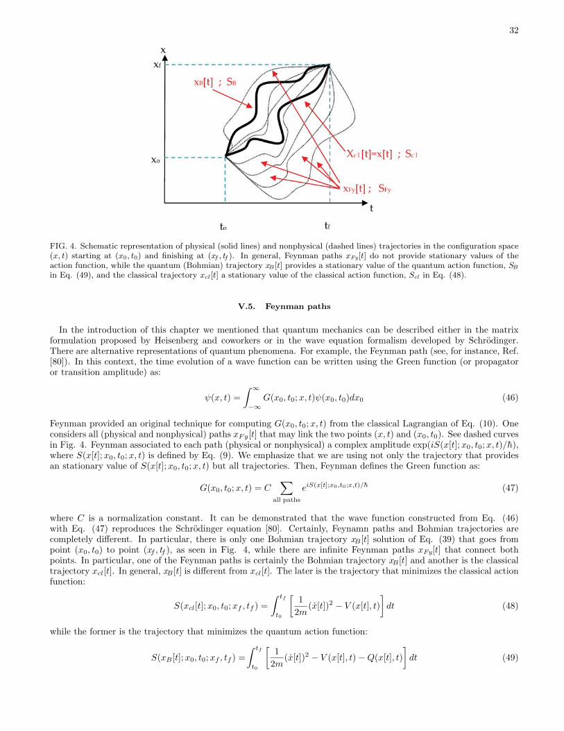
32

FIG. 4. Schematic representation of physical (solid lines) and nonphysical (dashed lines) trajectories in the configuration space(x, t) starting at (x0, t0) and finishing at (xf , tf ). In general, Feynman paths xFy[t] do not provide stationary values of theaction function, while the quantum (Bohmian) trajectory xB [t] provides a stationary value of the quantum action function, SBin Eq. (49), and the classical trajectory xcl[t] a stationary value of the classical action function, Scl in Eq. (48).

V.5. Feynman paths

In the introduction of this chapter we mentioned that quantum mechanics can be described either in the matrixformulation proposed by Heisenberg and coworkers or in the wave equation formalism developed by Schrodinger.There are alternative representations of quantum phenomena. For example, the Feynman path (see, for instance, Ref.[80]). In this context, the time evolution of a wave function can be written using the Green function (or propagatoror transition amplitude) as:

ψ(x, t) =

∫ ∞−∞

G(x0, t0;x, t)ψ(x0, t0)dx0 (46)

Feynman provided an original technique for computing G(x0, t0;x, t) from the classical Lagrangian of Eq. (10). Oneconsiders all (physical and nonphysical) paths xFy[t] that may link the two points (x, t) and (x0, t0). See dashed curvesin Fig. 4. Feynman associated to each path (physical or nonphysical) a complex amplitude exp(iS(x[t];x0, t0;x, t)/h),where S(x[t];x0, t0;x, t) is defined by Eq. (9). We emphasize that we are using not only the trajectory that providesan stationary value of S(x[t];x0, t0;x, t) but all trajectories. Then, Feynman defines the Green function as:

G(x0, t0;x, t) = C∑

all paths

eiS(x[t];x0,t0;x,t)/h (47)

where C is a normalization constant. It can be demonstrated that the wave function constructed from Eq. (46)with Eq. (47) reproduces the Schrodinger equation [80]. Certainly, Feynamn paths and Bohmian trajectories arecompletely different. In particular, there is only one Bohmian trajectory xB [t] solution of Eq. (39) that goes frompoint (x0, t0) to point (xf , tf ), as seen in Fig. 4, while there are infinite Feynman paths xFy[t] that connect bothpoints. In particular, one of the Feynman paths is certainly the Bohmian trajectory xB [t] and another is the classicaltrajectory xcl[t]. In general, xB [t] is different from xcl[t]. The later is the trajectory that minimizes the classical actionfunction:

S(xcl[t];x0, t0;xf , tf ) =

∫ tf

t0

[1

2m(x[t])2 − V (x[t], t)

]dt (48)

while the former is the trajectory that minimizes the quantum action function:

S(xB [t];x0, t0;xf , tf ) =

∫ tf

t0

[1

2m(x[t])2 − V (x[t], t)−Q(x[t], t)

]dt (49)

33

The derivation of the last expression can be straightforwardly obtained by repeating the steps done from the classicalaction function to the classical Hamilton–Jacobi equation but using now the quantum Hamilton–Jacobi equation. Weconclude that Bohmian trajectories are quite different from Feynman paths. The Bohmian trajectories are part of thebasic ontology of the theory, while the Feynman paths are basically a mathematical tool to compute the probabilities.

On the other hand, one could be interested in discussing whether the Feynman approach could be a more usefulcomputational tool than Bohmian mechanics for solving quantum systems. In principle, it seems that Feynman pathswould be less practical because we would have to compute an infinite number of trajectories from one particular initialposition and then repeat the procedure for all initial positions. On the contrary, in Bohmian mechanics we only needto compute one quantum trajectory for each initial position. See problems 15, 16 and 17.

V.6. Basic postulates for a single-particle

After introducing the reader to the language of trajectories for quantum mechanics (and wave functions for classicalmechanics), we can state the basic postulates of the Bohmian theory for a single particle. hey summarize in a fewsentences all the discussions held so far. In general, the postulates of any physical theory can be presented in differentcompatible ways. For example, classical mechanics can be postulated from Newton’s laws or Hamilton’s princi-ple. We follow here the standard presentation of Bohmian mechanics that involves a smaller number of ingredients[21, 24, 26, 72–74].

FIRST POSTULATE: The dynamics of a single particle in a single experiment in a quantum system is defined bya trajectory x[t] that moves continuously under the guidance of a wave function ψ(x, t). The wave function ψ(x, t) isa solution of the Schrodinger equation:

ih∂ψ(x, t)

∂t= − h2

2m

∂2ψ(x, t)

∂x2+ V (x, t) ψ(x, t)

The trajectory x[t] is obtained by time-integrating the particle velocity v[t] defined as:

v(x, t) =J(x, t)

|ψ(x, t)|2

where J(x, t) is the (ensemble) current density given by:

J(x, t) = ih

2m

(ψ(x, t)

∂ψ∗(x, t)

∂x− ψ∗(x, t)∂ψ(x, t)

∂x

)The initial position x[t0] and velocity v[t0] must be specified to completely determine the trajectory x[t].

SECOND POSTULATE (quantum equilibrium hypothesis): The initial position and velocity of a particular trajec-tory cannot be known with certainty. When the experiment is repeated many times ( j = 1, . . . , M ), the initial positionsxj [t0] of an ensemble of trajectories xj [t], associated to the same ψ(x, t), have to satisfy R2(x, t0) = |ψ(x, t0)|2,that is the number of trajectories of the ensemble between x and x + dx at the initial time t0 is proportional toR2(x, t0) = |ψ(x, t0)|2. The initial velocity of each trajectory is determined by vj [t0] = J(xj [t0], t0)/|ψ(xj [t0], t0)|2.

The condition on the distribution of the initial position in different experiments can be written mathematically as:

R2(x, t0) = limM→∞

1

M

M∑j=1

δ(x− xj [t0]) (50)

where j = 1, . . . ,M is the index of the different trajectories belonging to different experiments. If the set of M positionsof different experiments follows the distribution in Eq. (50) at the initial time t = 0, it is easy to demonstrate thatthe distribution of positions satisfies R(x, t)2 = |ψ(x, t)|2 at any time other time t:

R2(x, t) = limM→∞

1

M

M∑j=1

δ(x− xj [t]) (51)

provided that the many-particle wave function evolves according to the Schrodinger equation and that the particlesmove according to the corresponding Bohmian velocity, see problem 7. This property is known as equivariance [74, 77]

34

and it is key for the empirical equivalence between Bohmian mechanics and other quantum theories. Eq. (51) saysthat Born’s law is always satisfied by counting particles [24, 72–74]. Eq. (51) also explains why quantum results areunpredictable at the empirical arena [78].

The second postulate needs some additional remarks. It is argued by some authors that the second postulate, thequantum equilibrium hypothesis, is not a necessary postulate of the Bohmian theory. We will briefly explain thereasons in Sec. VI.5 when dealing with the postulates of a many particle system.

These postulates represent a minimalist explanation of the Bohmian interpretation of quantum mechanics withoutmentioning either the Hamilton–Jacobi equation, Eq. (39) or the quantum potential, Eq. (40). Certainly, we canformulate Bohmian mechanics without the use of the Hamilton–Jacobi formalism; however, in the authors’ opinion, thequantum Hamilton–Jacobi and the quantum potential allows us to improve our understanding of Bohmian mechanicsand provides clear arguments for discussing the similarities and differences between classical and quantum theories.Those who dislike the use of the quantum potential (and the quantum Hamilton–Jacobi equation) argue that itnaturally appears in the Schrodinger equation, but it is not present in other wave equations such as Dirac’s one. Onthe contrary, they state that the concept of Bohmian velocity, as defined in the first postulate, is much more generalbecause it is always present in any wave equation, as far as a local continuity equation for the probability density canbe established. This is true. However, in spite of this important limitation, we will show several times in this bookthat the quantum potential is a quite useful tool.

Finally, let us emphasize that no postulate about measurement is formulated here because, in Bohmian mechanics,no postulate about measurement is needed. For a more detailed explanation, please refer to Refs. [21, 24, 26, 72–74]and Sec. VII. In next section, we will explain how these postulates for single-particle systems are generalized tomany-particle systems.

VI. BOHMIAN MECHANICS FOR MANY-PARTICLE SYSTEMS

VI.1. Preliminary discussions: The many body problem

Up to now we have only studied a simple system composed of just one particle. However, a single-particle quantumsystem is some kind of crude idealization of any macroscopic or microscopic system found in nature, which is usuallyformed by a very large number of interacting particles. Strictly speaking, a single-particle system cannot be measured(one needs to consider the particles of the measuring apparatus that interact with the single-particle system). In thissection we will study nonrelativistic many-particle quantum systems with Bohmian trajectories. First of all, let usclarify the meaning of the term “many-particle” in Bohmian mechanics, as it can easily be misinterpreted. As we haveexplained in the previous section, we need an infinite ensemble of trajectories, M →∞, to describe the statistics of asingle-particle quantum system. These different trajectories should not be confused with different physical particlesof the system, since they all refer to different realizations (experiments) of the same single-particle quantum system.

Let us consider now a quantum system with N degrees of freedom, that is, an N body quantum system. We willuse a particular variable xk for each degree of freedom k = 1, . . . , N . The wave function will thus be a functionof all x1, . . . , xN variables. Now, a many-particle Bohmian trajectory will involve N interacting physical particlesx1[t], . . . , xN [t]. The relevant point that allows us to use the adjective “many-particle” is that the N particlesinteract between them, that is, the interacting potential depends on all possible particle positions, V (x1, . . . , xN ),in a non-trivial way. Along this section, in order to simplify our notation, we will use ~x[t] = (x1[t], . . . , xN [t]) or~x = (x1, . . . , xN ).

Now, an ensemble of identical experiments will be composed of M → ∞ Bohmian trajectories ~xj [t], with j =1, . . . ,M . The superscript j refers to the statistical index (counting experiments), while the subscript index will

refer to each of the N interacting particles present in each experiment, that is, ~xj [t] = (xj1[t], . . . , xjN [t]). In the restof chapter, we will use M to refer to the number of experiments and N to the number of physical particles of thequantum system in each experiment.

The first step to obtain the many-particle quantum trajectories is solving the following many-particle Schrodingerequation:

ih∂ψ(~x, t)

∂t=

(N∑k=1

− h2

2m

∂2

∂x2k

+ V (~x, t)

)ψ(~x, t) (52)

The solution ψ(~x, t) of this equation is the so-called many-particle wave function, that is defined in a N -dimensionalspace (plus time). The problem of N particles in a 1D space is formally equivalent to the one of a single particle in an

35

N -dimensional space. Here, we will use the term “many-particle” in a wide sense to include the single-particle N ≥ 2dimensional case.28

Equation (52) is analitically unsolvable most of the times, and its numerical integration is out of today’s presentcomputer capabilities, even for systems with N >∼ 5, since we need to compute the wave function ψ(~x, t) in the N -dimensional configuration space. Let us roughly estimate the hard disk space that we would require to store ψ(~x, t).Considering, for instance, a system with N = 10 particles confined in a 1D region of 10 nm, which we discretize with aspatial step of ∆x = 0.1 nm, we have a grid of 100 points for each dimension xk. Then, the total number of points inthe configuration space for the 10 particles is 10010 = 1020. Using 4 bytes (32 bits) to store the complex value of thewave function at each grid point, the information contained in a 10-particle wave function would require more than3 × 108 Terabytes (TB) (and more than 3 × 1028 TB for 20 particles). This practical limitation is the main reasonwhy our knowledge of many-particle quantum systems is so poor. This difficulty is the so-called many body problem.In 1929, Dirac wrote the following [81]:

The general theory of quantum mechanics is now almost complete. The underlying physical laws necessaryfor the mathematical theory of a large part of physics and the entire chemistry are thus completely known,and the difficulty is only that the exact application of these laws leads to equations much too complicatedto be soluble.

Three decades later, Born rephrased the issue [82]:

It would indeed be remarkable if Nature fortified herself against further advances in knowledge behind theanalytical difficulties of the many body problem.

The adjective “many-particle” can certainly be used with classical mechanics for N particles interacting throughV (~x, t). Now, it would be interesting to address the previous problem of storing the state of a 10-particle systembut now from the classical mechanics perspective. Solving the problem means finding the many-particle trajectory~xcl[t]. As discussed at the end of subsection 1.2.4, a classical many-particle trajectory can be computed alone, withoutknowing the rest of the trajectories of the ensemble (with different initial positions). At a computational level, thisfeature of classical mechanics implies a dramatic simplification. Basically, at each time step of the simulation, if theanalytical expression for the potential is known, we just need to save the position and velocity of each particle. Thismeans 20 real values for the 10-particle systems mentioned above. The classical trajectory of each particle, xcl

k [t], canbe obtained by solving a coupled system of Newton’s second laws:

mkd2xcl

k [t]

dt2=

[−∂V (~x, t)

∂xk

]~x=~xcl[t]

(53)

Fortunately, to compute a single classical trajectory ~xcl[t], we only need to evaluate the derivative of the many-particlepotential V (~x, t) along the trajectory. In the quantum case, even finding a single trajectory means solving for the entirewave function ψ(~x, t) that encapsulates the information of the entire ensemble of trajectories of all other experiments(the quantum wholeness).

In the scientific literature, there are many attempts to provide reasonable approximations to the many-body quan-tum problem. Density functional theory [83, 84] and the Hartree–Fock approximation [85–87] are some of the mostpopular techniques among the scientific community for dealing with the many body problem. In Sec. VI.1 we willdiscuss whether Bohmian trajectories can help in solving the many body problem. In what follows, we present thebasic theory of the many-particle Bohmian trajectories.

VI.2. Many-particle quantum trajectories

The efforts done in the single-particle section to compare classical and quantum mechanics are valid here. In par-ticular, we could write a classical (many-particle) wave equation or develop (many-particle) trajectories for quantumsystems. In this section, we will only explicitly develop the latter. We start by considering (nonrelativistic) spinlessparticles. In Sec. VI.4 we will introduce spin.

28 The variable N can be defined as the number of particles in a 1D space, or it can be related to the number of particles in a 3D space.In simple words, ψ(x1, x2, x3, t) can be interpreted as three particles in a 1D space or just one particle in a 3D space. From a physicalpoint of view, one particle in a 3D space is a “single-particle” system. However, from the computational point of view, it is equivalentto a three-particle system in 1D.

36

VI.2.1. Many-particle continuity equation

Following a similar development as we did for the single-particle case, see Sec. V.3, we can derive the followinglocal continuity equation associated to the many-particle Schrodinger equation, Eq. (52):

∂|ψ(~x, t)|2

∂t+

N∑k=1

∂

∂xkJk(~x, t) = 0 (54)

where we have defined

Jk(~x, t) = ih

2m

(ψ(~x, t)

∂ψ∗(~x, t)

∂xk− ψ∗(~x, t)∂ψ(~x, t)

∂xk

)(55)

as the k-th component of the current density, see problem 7.Since the many-particle Schrodinger equation is also compatible with a local conservation of particles, we can

interpret |ψ(~x, t)|2 as the spatial distribution of an ensemble of many-particle trajectories assigned to an ensemble ofdifferent experiments. The Bohmian velocity of the k-th trajectory is:

vk(~x, t) =Jk(~x, t)

|ψ(~x, t)|2(56)

In fact, the strategy followed here to develop Bohmian mechanics can be extended to any quantum equation of motionwhere a continuity equations holds: first, look for a continuity equation for the probability density and, then, define avelocity for the Bohmian trajectories as the current density divided by the probability density. A particular examplewill be developed for particles with spin in Sec. VI.4 and chapter 8.

VI.2.2. Many-particle quantum Hamilton–Jacobi equation

Alternatively, we can obtain Bohmian mechanics from a quantum Hamilton–Jacobi equation. We start by introduc-ing the polar form of the many-particle wave function ψ(~x, t) = R(~x, t)eiS(~x,t)/h into the many-particle Schrodingerequation, Eq. (52). Then, after a quite simple manipulation, one obtains from the imaginary part:

∂R2(~x, t)

∂t+

N∑k=1

∂

∂xk

(1

m

∂S(~x, t)

∂xkR2(~x, t)

)= 0 (57)

where we recognize the velocity of the k-th particle as:

vk(~x, t) =1

m

∂S(~x, t)

∂xk(58)

Equations (56) and (58) are identical. This is shown in problem 6 for a 1D system, but it can straightforwardlybe generalized to N dimensions. The real part of the Schrodinger equation leads to a many-particle version of thequantum Hamilton–Jacobi equation:

∂S(~x, t)

∂t+

N∑k=1

1

2m

(∂S(~x, t)

∂xk

)2

+ V (~x, t) +Q(~x, t) = 0 (59)

where we have defined the quantum potential as:

Q(~x, t) =

N∑k=1

Qk(~x, t) (60)

with:

Qk(~x, t) = − h2

2m

∂2R(~x, t)/∂x2k

R(~x, t)(61)

37

Again, we can obtain a system of coupled Newton-like equations (one for each component of ~x) for the many-particleBohmian trajectories by computing the time-derivative of the Bohmian velocity of Eq. (56):

md2xk[t]

dt2=

[− ∂

∂xk(V (~x, t) +Q(~x, t))

]~x=~x[t]

(62)

Both the potential V (~x, t) and the quantum potential Q(~x, t) introduce correlations between particles. All physicalinteractions are essentially expressed as correlations (relations) between the degrees of freedom. In the following, wewill discuss some important differences between classical and quantum correlations.

VI.3. Factorizability, entanglement, and correlations

There are important differences between the correlations introduced by the classical potential V (~x, t) and thequantum potential Q(~x, t):

1. In general, the term V (~x, t) decreases with the distance between particles. A simple example is the Coulombinteraction. However, Q(~x, t) depends only on the shape of the wave function, not on its value (see Eq. (61)).Thus, the quantum potential that we would obtain from Eq. (61) using either R(~x, t) or aR(~x, t) would beexactly the same, even when a → 0. Thus, the quantum potential can produce a significative interactionbetween two particles, even if they are very far apart.29

2. In general, the term V (~x, t) produces classical correlations between different particles. The particular depen-dence of V (~x, t) in all variables x1, . . . , xN imposes a restriction on the speed of the interaction. The variationsof xi can only affect xj after a time larger than |xi − xj |/c, c being the speed of light. For example, therelation between the particles positions in the electromagnetic interactions ensures that there is no superluminalinfluence between particles. However, such a restriction is not present in the quantum potential. Thus, very farparticles have an instantaneous (nonlocal) interaction between them.

The quantum potential is at the origin of all quantum correlations, that is, entanglement, that can imply (nonlocal)faster-than-light interactions when two distant particles are involved. As mentioned in Sec. IV.5, this “spooky actionat a distance” is what bothered Einstein about Bohmian mechanics (and quantum mechanics, in general). In 1964,Bell elaborated his famous theorem that established clear experimentally testable mathematical inequalities thatwould be fulfilled by local theories but would be violated by nonlocal ones [50]. All experimental results obtainedso far confirm that Bell’s inequalities are violated. Therefore, contrarily to Einstein’s belief, we have to acceptthe real existence, in nature, of faster-than-light causation.30 Entanglement is an intrinsic correlation in quantummechanics (whose complexity and potentialities eventually come from the fact that a N -particle wave function lives ina N -dimensional configuration space) and is at the core of quantum information science, which makes teleportation,quantum communication, quantum cryptography, and quantum computing possible.

To improve our understanding of correlations, let us discuss under which conditions we cannot expect correlationsbetween N particles. Let us focus our attention on a wave function ψ(~x, t) that can be written as a product ofsingle-particle wave functions associated with each of the particles:

ψ(~x, t) =

N∏k=1

ψk(xk, t) (63)

We call such a wave function “factorizable” or “separable”. Equation (63) expresses the physical independence of theNparticles (even though the wave functions ψk(xk, t) may overlap). According to Born’s statistical interpretation of wavefunctions, the squared modulus of a wave function is the probability density of the quantum particle; thus the quantumwave function, Eq. (63), corresponds to a system without (classical or quantum) correlations between particles. It iswell known that such a solution occurs when the potential in Eq. (52) can be written as V (~x) =

∑k Vk(xk). Next,

let us reformulate this result with Bohmian trajectories.We realize that the phase and modulus of Eq. (63) are given by:

S(~x, t) =

N∑k=1

Sk(xk, t) (64)

29 These highly nonclassical features of the quantum potential is what led Bohm to argue that the quantum potential interchangesinformation between systems [23, 28].

30 We insist that the experimental violation of Bell’s inequalities gives direct support not only to the Copenhagen interpretation but alsoto the Bohmian one, since the latter is also a nonlocal theory because of the presence of Q(~x, t).

38

and

R(~x, t) =

N∏k=1

Rk(xk, t) (65)

by defining

ψk(xk, t) = Rk(xk, t)eiSk(xk,t)/h (66)

In this case, the many-particle quantum potential can be written as:

Qk(~x, t) = − h2

2m

∂2Rk(xk, t)/∂x2k

Rk(xk, t)(67)

Then, we can easily deduce from Eq. (59) that each ψk(xk, t) is a solution of the following single-particle quantumHamilton–Jacobi equation:

∂Sk(xk, t)

∂t+

1

2m

(∂Sk(xk, t)

∂xk

)2

+ V (xk, t) +Qk(xk, t) = 0 (68)

In addition, each ψk(xk, t) satisfies a conservation law:

∂R2k(xk, t)

∂t+

∂

∂xk

(1

m

∂Sk(xk, t)

∂xkR2k(xk, t)

)= 0 (69)

From these equations we can easily deduce an independent guiding equation for each k-particle:

mdxk[t]

dt=

(∂Sk(xk, t)

∂xk

)xk=xk[t]

(70)

showing the absence of correlations between (the different components of the many-particle) Bohmian trajectory.

VI.4. Spin and identical particles

Elementary particles, such as electrons or quarks, have spin, an internal (discrete) degree of freedom that caninfluence their quantum dynamics in a nontrivial manner. In this section we will briefly explain how to extend(nonrelativistic) Bohmian mechanics to include spin.

VI.4.1. Single-particle with s = 1/2

In the orthodox formulation of quantum mechanics, the state of a single particle with spin s is described by a 2s+1component vector of wave functions with:

~Ψ(~r, t) =

Ψ1(~r, t)...

Ψ2s+1(~r, t)

(71)

where ~r = (x1, x2, x3) represents the 3D position of the particle. The time evolution of this state is no longer governedby the Schrodinger equation but by more involved wave equations such as the Pauli equation for s = 1/2 [62, 88, 89].

The strategy to find Bohmian trajectories for spin particles will be the following: we will look for a continuityequation of the probability density and define the Bohmian velocity as the current density divided by the probabilitydensity. The idea is quite simple, but the mathematical development can be much more complicated. Therefore, wewill focus on a particular example for a spin s = 1/2 charged particle, whose vectorial wave function,

~Ψ(~r, t) =

(Ψ↑(~r, t)Ψ↓(~r, t)

)(72)

39

has two components and it is called a spinor. In this particular case, the spin along a particular direction takes onlytwo possible values, referred to as spin-up (↑) and spin-down (↓) states. The time evolution is given by the Pauliequation [62]:

ih∂

∂t~Ψ(~r, t) =

[1

2m~σ ·(−ih~∇− q ~A(~r, t)

)2

+ V (~r, t)

]~Ψ(~r, t) (73)

where ~σ = (σ1, σ2, σ3) is a vector containing the Pauli matrices [88]:

σ1 =

(0 11 0

)(74)

σ2 =

(0 −ii 0

)(75)

σ3 =

(1 00 −1

)(76)

and V (~r, t)/q and ~A(~r, t) = (A1(~r, t), A2(~r, t), A3(~r, t)) are, respectively, the electromagnetic scalar and vector poten-tial.

From the Pauli equation we obtain a continuity equation:

∂ρ(~r, t)

∂t+ ~∇ ~J(~r, t) = 0 (77)

with the probability and current densities defined as:

ρ(~r, t) = ~Ψ†(~r, t) · ~Ψ(~r, t) (78)

~J(~r, t) = ih

2m

(~Ψ(~r, t) · ~∇~Ψ†(~r, t)− ~Ψ†(~r, t) · ~∇~Ψ(~x, t)

)−

~A(~r, t)

mcρ(~r, t), (79)

where ~Ψ† denotes the conjugate transpose of ~Ψ.Defining the Bohmian velocity as:

~v(~r, t) =~J(~r, t)

ρ(~r, t)(80)

one can develop Bohmian trajectories for spin particles. Notice that the spin is basically a property defined throughthe wave function of the particle, not through its position. In any case, since the Bohmian velocity of the particleis affected by the wave function, the spin can have a direct effect on the trajectory. 31 It is out of the scope of thisbook to further develop Bohmian mechanics for the Pauli equation. In any case, practical examples of the particletrajectories for spin-1/2 particles can be found in Refs. [71, 89].

The Pauli equation can be rewritten as:

ih∂

∂t~Ψ(~r, t) =

[1

2m

(−ih~∇− q ~A(~r, t)

)2

− hq

2m~σ · ~B(~r, t) + V (~r, t)

]~Ψ(~r, t) (81)

~B(~r, t) = ~∇ × ~A(~r, t) being the magnetic field. Note that the only term that can transfer population between spin

states is the one with ~B (the so-called Stern–Gerlach term). If this term can be neglected then each spin componentof Eq. (81) reduces to the familiar Schrodinger equation.

On the other hand we can also consider the case where the Hamiltonian is separable into a part depending only onthe particle position and a part depending only on the spin. Then if the initial state is:

~Ψ(~r, 0) = ψ(~r, 0)

(α↑(0)α↓(0)

)(82)

31 Alternatively, one could also consider the degree of freedom of spin as an additional three-angle variable α, β, γ of the wave function(such that R(~r, α, β, γ, t) and S(~r, α, β, γ, t)) and look for the equations of motion of the trajectories of the positions and also of thetrajectories of the angles (see chapter 10 in Ref. [24]).

40

at later times one can write the spinor evolution in a simpler form as:

~Ψ(~r, t) = ψ(~r, t)

(α↑(t)α↓(t)

)≡ ψ(~r, t)~χ(t) (83)

where ψ(~r, t) depends only on the coordinate of the particles and the function ~χ(t) depends only on its spin. We callthe former the coordinate or orbital wave function and the latter the spin wave function. In this case, the evolutionof ~χ(t) and ψ(~r, t) is independent. If we are not interested in the actual spin of the particles, we can just consider thedynamics of the coordinate function ψ(~r, t), which will be determined by the Schrodinger equation.

VI.4.2. Many-particle system with s = 1/2 particles

For a nonrelativistic system of many particles, where the orbital and spin contributions of the Hamiltonian areinitially separable,32 the many-particle wave function will be also separable at all times, that is:

Ψ(~r1, . . . ~rN , t) = ψ(~r1, . . . ~rN , t)~χ(t) (84)

where ψ(~r1, . . . ~rN , t) is the time evolution of the orbital state, the solution of the many-particle Schrodinger equation,and ~χ(t) is the time evolution of the spin part of the system state:

~χ(t) =

α↑1↑2...↑N (t)α↑1↑2...↓N (t)

...α↓1↓2...↓N (t)

=

α1(t)α2(t)

...αW (t)

(85)

W ≡ (2s+ 1)N is the number of possible combinations of spin projections in one direction for all the particles in thesystem.33

In many practical situations, we are only interested in the evolution of the orbital wave function through the many-particle Schrodinger equation. However, even in this case, there is a peculiar dependence of the dynamics of theparticles on the total spin. As explained in many textbooks, there is a pure quantum interaction between identicalparticles, named “exchange interaction” [88, 90]. This interaction is not classical, and we cannot find a term in thepotential energies of the many-particle Hamiltonian of the Schrodinger equation that accounts for it. Alternatively,this new interaction is introduced in the “shape” of the global wave function, through the requirement of a particularsymmetry. We say that a many-particle wave function is anti-symmetric when the interchange of the position andspin degrees of freedom associated to two identical fermions (e.g., electrons) results only in a change of the sign of

the global wave function, ~Ψ(~r1, ~r2, . . . , ~rN , t). Analogously, we say that the many-particle wave function is symmetricwhen it remains unchanged after the interchange of the degrees of freedom of two identical bosons.

The crucial point why we cannot forget about spin when dealing with many-particle Hamiltonians is that forseparable wave functions, for example, Eq. (84), the symmetry of the orbital part depends on the symmetry of thespin part. For example, since the total wave function must be antisymmetric, two electrons can have a symmetricorbital part if the spin part is antisymmetric, and vice versa. In general, note that the wave function is not separable,and it makes no sense to talk about the symmetry of the orbital and spin parts alone but only of the symmetry ofthe total wave function. We see that the exchange interaction induces correlations between particles by imposingsymmetries (or shapes) to their many-particle wave function.

A standard claim in many quantum mechanics textbooks is that identical particles, for example, two electrons withan antisymmetric wave function, are indistinguishable. It is affirmed that if the particles would have trajectories,they would automatically be distinguishable. In Bohmian mechanics, even with the symmetrization postulate, theadjective “indistinguishable” is inappropriate because one can label one particle’s trajectory ~r1[t] and the other ~r2[t]and thus distinguish them perfectly at the ontological staff.

Bohmian trajectories can actually help us improve our understanding of the symmetrization postulate. Let usassume a two-electron system with an antisymmetric orbital wave function ψ(~r1, ~r2, t). We assume that an electron

32 For example, in the absence of a magnetic field such that the initial wave function can be written as a product of an orbital part,ψ(~r1, ~r2, . . . ~rN , 0), and a spin part, ~χ(0).

33 Additionally, one can also look for the projection of the total spin of the system. Both procedures are connected by the Clebsch–Gordancoefficients [88].

41

labeled 1 with the initial position ~r1[0] evolves into ~r1[t] and an another electron labeled 2 evolves from ~r2[0] to~r2[t]. Then, it can be easily understood that ~r1

′[0] = ~r2[0] evolves into ~r1′[t] = ~r2[t] and ~r2

′[0] = ~r1[0] evolvesinto ~r2

′[t] = ~r1[t]. We use primes to notice that ~r1[t] and ~r1′[t] correspond to trajectories of the same particle with

different initial positions (~r1[0] or ~r2[0]). This result follows from the symmetry of the velocity, that is, the symmetryof the current density and modulus, when positions of the two electrons are interchanged. In summary, Bohmiantrajectories of identical particles are clearly distinguishable in our computation, but the observable (ensemble) resultsobtained from them are indistinguishable when we interchange their initial positions. Hence in Bohmian mechanicsa set of particles with exchange symmetry are perfectly distinguishable at the ontological plane, while they becomeindistinguishable at the empirical plane.

VI.5. Basic postulates for many-particle systems

The basic postulates of Bohmian mechanics for many-particle systems are exactly the same as those we havedeveloped for a single particle but adding the symmetrization postulate. As done in Sec. V.6, we also present aminimalist formulation of the postulates.

In order to simplify our description, we assume the simpler many-particle wave function written as:

~Ψ(~r1, . . . , ~rN , t) = ψ(~r1, . . . , ~rN , t)

↑1↑2 . . . ↑N (t)

0...0

(86)

The generalization of the present postulates to include the more general wave functions of Eq. (84) follows straight-forwardly.

FIRST POSTULATE: The dynamics of a many-particle quantum system comprises a wave function, Eq. (86),whose orbital part ψ(~r1, ~r2, . . . , ~rN , t) is defined in the configuration space ~r1, ~r2, . . . , ~rN plus time, and a many-particle trajectory ~r1[t], ~r2[t], . . . , ~rN [t] that moves continuously under the guidance of the wave function.

The orbital part of the wave function ψ(~r1, ~r2, . . . , ~rN , t) is a solution of the many-particle Schrodinger equation:

ih∂ψ(~r1, . . . , ~rN , t)

∂t=

(N∑k=1

− h2

2m∇2~rk

+ V (~r1, . . . , ~rN , t)

)ψ(~r1, . . . , ~rN , t)

Each component ~rk[t] of the many-particle trajectory ~r1[t], . . . , ~rN [t] is obtained by time-integrating the particlevelocity ~vk[t] = ~vk(~r1, . . . , ~rN , t) defined from:

~vk(~r1, . . . , ~rN , t) =~Jk(~r1, . . . , ~rN , t)

|ψ(~r1, . . . , ~rN , t)|2

where |ψ(~r1, . . . , ~rN , t)|2 = ψ(~r1, . . . , ~rN , t)ψ∗(~r1, . . . , ~rN , t) is the square modulus of the wave function and ~Jk =

~Jk(~r1, . . . , ~rN , t) is the k-particle current density :

~Jk = ih

2m

(ψ(~r1, .., ~rN , t)~∇~rkψ∗(~r1, .., ~rN , t)− ψ∗(~r1, .., ~rN , t)~∇~rkψ(~r1, .., ~rN , t)

)The initial positions ~r10, ~r20, . . . , ~rN0 and velocities ~v10, ~v20, . . ., ~vN0 have to be specified in order to completelydetermine the many-particle trajectory.

SECOND POSTULATE (quantum equilibrium hypothesis): The initial positions ~rj1[t0], ~rj2[t0], . . . , ~rjN [t0] and

velocities ~vj1[t0], ~vj2[t0], . . ., ~rjN [t0] of a particular many-particle j trajectory cannot be known with certainty. Whenthe experiment is repeated many times, these initial positions of an ensemble of trajectories associated with the sameψ(~r1, . . . , ~rN , t) satisfy that the number of trajectories of the ensemble between (~r1, . . . , ~rN ) and (~r1+d~r1, . . . , ~rN+d~rN )

at the initial time t0 is proportional to R2(~rj1[t0], . . . , ~rjN [t0]) = |ψ(~rj1[t0], . . . , ~rjN [t0], t0)|2. The initial velocity is deter-

mined by ~vjk[t0] = ~Jk(~rj1[t0], . . . , ~rjN [t0], t0)/|ψ(~rj1[t0], . . . , ~rjN [t0], t0)|2 .

42

The condition on the initial position can be written mathematically as:

R2(~r1, . . . , ~rN , t0) = limM→∞

1

M

M∑j=1

N∏k=1

δ(~r − ~rjk[t0]) for t = t0 (87)

Notice the presence of two indices, the j = 1, . . . ,M for the infinite ensemble of identical experiments and thek = 1, . . . , N for the N degrees of freedom.

THIRD POSTULATE (symmetrization postulate of quantum mechanics): If the variables ~ri, ↑i and ~rj , ↑j refer totwo identical particles of the ensemble, then the wave function, Eq. (86), is either symmetric:

ψ(., ~ri, ., ~rj , ., t)

↑i . . . ↑j . . .

0...0

= ψ(., ~rj , ., ~ri, ., t)

↑j . . . ↑i . . .

0...0

(88)

if the particles are bosons (every particle with an integer spin 0, 1, 2, . . . is a boson), or antisymmetric:

ψ(., ~ri, ., ~rj , ., t)

↑i . . . ↑j . . .

0...0

= −ψ(., ~rj , ., ~ri, ., t)

↑j . . . ↑i . . .

0...0

(89)

if the particles are fermions (every particle with a half-odd spin 1/2, 3/2, . . . is a fermion). In Eq. (88) and Eq. (89)it is understood that all other degrees of freedom of the other particles remain unchanged.34

As we already did in the development of the postulates for a single-particle system, we remind that the secondpostulate needs some additional remarks since it has been argued by some authors that this postulate, the quantumequilibrium hypothesis, is not a necessary postulate of the Bohmian theory.

First, it has been demonstrated that if one assumes that the many-particle wave function of the whole Universe,the so-called Universal wave function that includes all degrees of freedom of the Universe, satisfies some (typical)conditions then, it follows that each (conditional) wave function of each quantum (sub) system will satisfy its ownEq. (87). Thus, the justification about the quantum equilibrium postulate has to be done only for the Universal wavefunction, not for each individual (sub)system.

Probably, the most accepted view against taking the quantum equilibrium as a postulate comes from the seminalwork by Durr, Goldstein, and Zanghı [74, 77], where the equivariance in any system is discussed from the initialconfigurations of (Bohmian) particles in the Universe. Using Bohmian mechanics to describe the wave function of thewhole Universe, then the wave function associated to any (sub)system is an effective (conditional) wave function ofthe universal one. Using typicality arguments, they showed that the overwhelming majority of possible selections ofinitial positions of particles in the Universe will satisfy Eq. (87) in a subsystem (or Eq. (51) for a subsystem withone degree of freedom) [74, 77]. Other authors [91] have attempted to dismiss Eq. (87) as a postulate by showingthat any initial configuration of Bohmian particles will relax, after some time, to a distribution very close to Eq. (51)for a subsystem. Such discussions about quantum equilibrium are far from the scope of this book. Therefore, froma practical point of view, one can postulate Eq. (87) (at some initial time) in the Bohmian theory in the same waythat Born’s law is a postulate in the orthodox theory.

Again, no postulate about measurement is needed, since in Bohmian mechanics measurement is treated as aparticular case of interaction between particles (see Sec. VII).

VI.6. The conditional wave function: many-particle Bohmian trajectories without the many-particle wavefunction

In section 1.2.4, when discussing the similarities and differences between classical and quantum mechanics, wementioned quantum wholeness (the dependence of each individual Bohmian trajectory on the rest of trajectories

34 This simple spin vector wave function is clearly symmetric so that the orbital wave function has to be either symmetric or antisymmetric.For general wave functions, such as the one in Eq. (84), this postulate implies much more complicated restrictions on the possible orbitaland spin wave functions.

43

through the wave function) as a fundamental difference. This concept acquires an even more dramatic meaning when

dealing with many-body systems. A particular Bohmian trajectory of the k-particle ~rjk[t] depends on the rest of infinitej = 1, . . . ,M possible trajectories (with different initial position associated to different experiments) of all k = 1, . . . , Nparticles (corresponding to the N degrees of freedom of the quantum system). This property is mathematicallymanifested by the fact that the many-particle wave function is defined in an N -dimensional configuration space ratherthan in the usual real 3D real space. In a 3D real space one can easily define whether or not two particles are faraway. In general, the potential profile that determines the interaction between these two particles decreases with thedistance. However, two distant particles that share a common region of the N -dimensional configuration space wherethe wave function is different from zero have an interaction (entanglement) independently of their distance.

As discussed in section Sec. VI.1, the need of computing the many-particle wave function in the N -dimensionalconfiguration space is the origin of the quantum many-body problem. Among the large list of approximations presentin the literature to tackle this problem, Bohmian mechanics provides a natural, original and mainly unexplored solutionthrough the use of the conditional wave function [92]. Due to the Bohmian dual description of a quantum system asparticles and waves, one can reduce the complexity of a many-particle wave function through the substitution of someof the N degrees of freedom by its corresponding Bohmian trajectories. The new wave function with a reduced numberof degrees of freedom is named conditional wave function. For a discussion about the fundamental implications ofworking with conditional wave functions instead of full many-body wave functions, see Refs [92, 93]. We will presentnow some work on the computational abilities of such conditional wave functions.

Hereafter, for simplicity, we return to a definition of the degrees of freedom of the many-particle quantum sys-tem in terms of x1, x2, . . . , xN instead of ~r1, ~r2, . . . , ~rN. The direct solution of the many-particle Schrodingerequation, Eq. (52), is intractable numerically. On the contrary, differential classical equations of motion deal withsolutions in a much smaller configuration space, x1[t], . . . , xi−1[t], xa, xi1[t], . . . , xN [t], where all other trajectoriesare known parameters, except xa. In other words, the Newton solution of xa[t] just needs the spatial dependence ofV (x1[t], . . . , xa, . . . , xN [t]) on the variable xa. In this section, we summarize the formalism developed by Oriols [94] tocompute many-particle Bohmian trajectories without knowing the many-particle wave function. It is a clear exampleof how Bohmian mechanics can be a powerful computational tool.

The main idea behind the work developed in [94] is that any Bohmian trajectory xa[t] that is computed fromthe many-particle wave function Ψ(~x, t) solution of Eq. (52) can be alternatively computed from a much simplersingle-particle conditional wave function φa(xa, t) = Ψ(xa, ~xb[t], t). Here, we use the notation ~x = xa, ~xb with~xb = x1, . . . , xa−1, xa+1, . . . , xN for particle positions and ~xb[t] = x1[t], . . . , xa−1[t], xa+1[t], . . . , xN [t] for Bohmiantrajectories.

It is quite trivial to demonstrate the ability of φa(xa, t) in reproducing xa[t]. By construction, when we use apolar form φa(xa, t) = ra(xa, t) e

i sa(xa,t)/h, the angle sa(xa, t) is identical to the angle S(xa, ~xb, t) of Ψ(xa, ~xb, t)evaluated at xa, ~xb[t]. Therefore, since the velocity of the trajectory xa[t] is computed from the spatial dependenceof S(xa, ~xb, t) on xa when all other positions are fixed at ~xb = ~xb[t], the same velocity will be obtained from thespatial dependence of sa(xa, t). Interestingly, φa(xa, t) is solution of a single-particle (pseudo) Schrodinger equationbecause it depends only on time t and position xa. Next, our effort will be focused on determining such single-particleequations.

VI.6.1. Single-particle pseudo-Schrodinger equation for many-particle systems

First of all, we show that any (totally arbitrary) single-valued complex function φa(xa, t), which has a well-definedsecond-order spatial derivative and first-order temporal derivative, can be obtained from a Schrodinger-like equationwhen the following potential W (xa, t) is used:

W (xa, t) =ih∂φa(xa,t)

∂t + h2

2m∂2φa(xa,t)

∂2xa

φa(xa, t)(90)

For an arbitrary (complex) function, the potential energy W (xa, t) can be complex, too. In fact, we are interested inrewriting W (xa, t) in terms of the polar form of the wave function φa(xa, t) = ra(xa, t) e

i sa(xa,t)/h. We obtain for thereal part:

Real[W (xa, t)] = −

(1

2 m

(∂sa(xa, t)

∂xa

)2

− h2

2 m ra(xa, t)

∂2ra(xa, t)

∂2xa+∂sa(xa, t)

∂t

)(91)

44

From Eq. (90), we do also obtain for the imaginary part:

Imag[W (xa, t)] =h

2r2a(xa, t)

(∂r2a(xa, t)

∂t+

∂

∂xa

(r2a(xa, t)

m

∂sa(xa, t)

∂xa

))(92)

It can be easily verified that Imag[W (xa, t)] = 0 when the single-particle wave function preserves the norm.Finally, we are interested in using the above expressions when the single-particle wave function is the one mentioned

in the introduction of this subsection, φa(xa, t) = Ψ(xa, ~xb[t], t). In particular, we use ra(xa, t) = R(xa, ~xb[t], t) andsa(xa, t) = S(xa, ~xb[t], t). Then, we realize that Eq. (90) transforms into:

ih∂φa(xa, t)

∂t=

(− h2

2m

∂2

∂2xa+ Ua(xa, ~xb[t], t) +Ga(xa, ~xb[t], t) + iJa(xa, ~xb[t], t)

)φa(xa, t)

(93)

where we have defined:

Ga(~x, t) = Ub(~xb, t) +

N∑k=1;k 6=a

(1

2 m

(∂S(~x, t)

∂xk

)2

+Qk(~x, t)− ∂S(~x, t)

∂xkvk(~x[t], t)

)(94)

with Qk(~x, t) as the quantum potential energy defined in Eq. (61). The terms Ua(xa, ~xb[t], t) and Ub(~xb, t) are definedfrom the many-particle potential that appears in the original many-particle potential energy in Eq. (52) as:

V (~x, t) = Ua(xa, ~xb, t) + Ub(~xb, t) (95)

In addition, we have defined:

Ja(~x, t) =

N∑k=1;k 6=a

h

2R2(~x, t)

(∂R2(~x, t)

∂xkvk(~x[t], t)− ∂

∂xk

(R2(~x, t)

m

∂S(~x, t)

∂xk

))(96)

In order to obtain these expressions, one has to carefully evaluate:

∂S(xa, ~xb[t], t)

∂t=

(∂S(xa, ~xb, t)

∂t

)~xb=~xb[t]

+

N∑k=1;k 6=a

∂S(xa, ~xb[t], t)

∂xkvk(~x[t], t)

(97)

and use Eq. (59) evaluated at xa, ~xb[t]. Identically for ∂R2(xa, ~xb[t], t)/∂t with Eq. (57).The single-particle pseudo-Schrodinger equation, Eq. (93), is the main result of this algorithm. Let us discuss the

role of each potential term in Eq. (93):

1. The term Ua(xa, ~xb[t], t) is a real-valued potential whose explicit dependence on the positions is known. It hasto be evaluated from the particular Bohmian position of all particles except xa[t].

2. The term Ga(xa, ~xb[t], t) is a real-valued potential whose explicit dependence on the positions is unknown (unlesswe know the many-particle wave function) and needs some educated guess. It takes into account, for example,the exchange interaction between particles.

3. The term iJa(xa, ~xb[t], t) is an imaginary-valued potential whose explicit dependence on the positions is alsounknown and needs some educated guess. It takes into account that the norm of φa(xa, t) is not directlyconserved (the norm of the many-particle wave function Ψ(xa, ~xb, t) is conserved in the entire configurationspace, but this is not true for Ψ(xa, ~xb[t], t) in the xa space).

By using Eq. (93) for each particle, xa[t] for a = 1, . . . , N , we obtain a system of N coupled single-particle pseudo-Schrodinger equations that is able to compute many-particle Bohmian trajectories without knowing the many-particlewave function. The great merit of Eq. (93) is to demonstrate that such a single-particle solution of a many-particleproblem exists, although we do not know exactly the values of the terms Ga(xa, ~xb[t], t) and Ja(xa, ~xb[t], t). Ouralgorithms have similarities with the original work on density functional theory [83, 84]. The formidable computationalsimplification comes at the price that some terms of the potential of the corresponding single-particle Schrodingerequations are unknown, that is, the exchange-correlation functional in density functional theory [83, 84] and, here,the terms in Eqs. (94) and (96).

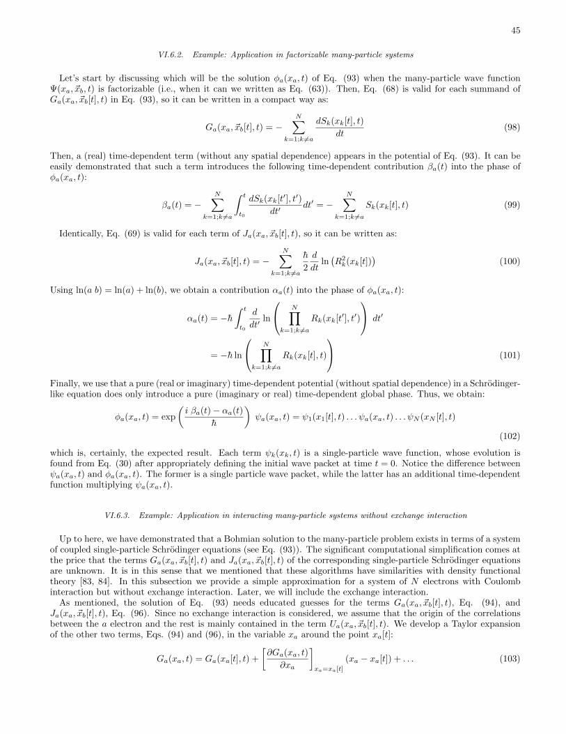
45

VI.6.2. Example: Application in factorizable many-particle systems

Let’s start by discussing which will be the solution φa(xa, t) of Eq. (93) when the many-particle wave functionΨ(xa, ~xb, t) is factorizable (i.e., when it can we written as Eq. (63)). Then, Eq. (68) is valid for each summand ofGa(xa, ~xb[t], t) in Eq. (93), so it can be written in a compact way as:

Ga(xa, ~xb[t], t) = −N∑

k=1;k 6=a

dSk(xk[t], t)

dt(98)

Then, a (real) time-dependent term (without any spatial dependence) appears in the potential of Eq. (93). It can beeasily demonstrated that such a term introduces the following time-dependent contribution βa(t) into the phase ofφa(xa, t):

βa(t) = −N∑

k=1;k 6=a

∫ t

t0

dSk(xk[t′], t′)

dt′dt′ = −

N∑k=1;k 6=a

Sk(xk[t], t) (99)

Identically, Eq. (69) is valid for each term of Ja(xa, ~xb[t], t), so it can be written as:

Ja(xa, ~xb[t], t) = −N∑

k=1;k 6=a

h

2

d

dtln(R2k(xk[t])

)(100)

Using ln(a b) = ln(a) + ln(b), we obtain a contribution αa(t) into the phase of φa(xa, t):

αa(t) = −h∫ t

t0

d

dt′ln

N∏k=1;k 6=a

Rk(xk[t′], t′)

dt′

= −h ln

N∏k=1;k 6=a

Rk(xk[t], t)

(101)

Finally, we use that a pure (real or imaginary) time-dependent potential (without spatial dependence) in a Schrodinger-like equation does only introduce a pure (imaginary or real) time-dependent global phase. Thus, we obtain:

φa(xa, t) = exp

(i βa(t)− αa(t)

h

)ψa(xa, t) = ψ1(x1[t], t) . . . ψa(xa, t) . . . ψN (xN [t], t)

(102)

which is, certainly, the expected result. Each term ψk(xk, t) is a single-particle wave function, whose evolution isfound from Eq. (30) after appropriately defining the initial wave packet at time t = 0. Notice the difference betweenψa(xa, t) and φa(xa, t). The former is a single particle wave packet, while the latter has an additional time-dependentfunction multiplying ψa(xa, t).

VI.6.3. Example: Application in interacting many-particle systems without exchange interaction

Up to here, we have demonstrated that a Bohmian solution to the many-particle problem exists in terms of a systemof coupled single-particle Schrodinger equations (see Eq. (93)). The significant computational simplification comes atthe price that the terms Ga(xa, ~xb[t], t) and Ja(xa, ~xb[t], t) of the corresponding single-particle Schrodinger equationsare unknown. It is in this sense that we mentioned that these algorithms have similarities with density functionaltheory [83, 84]. In this subsection we provide a simple approximation for a system of N electrons with Coulombinteraction but without exchange interaction. Later, we will include the exchange interaction.

As mentioned, the solution of Eq. (93) needs educated guesses for the terms Ga(xa, ~xb[t], t), Eq. (94), andJa(xa, ~xb[t], t), Eq. (96). Since no exchange interaction is considered, we assume that the origin of the correlationsbetween the a electron and the rest is mainly contained in the term Ua(xa, ~xb[t], t). We develop a Taylor expansionof the other two terms, Eqs. (94) and (96), in the variable xa around the point xa[t]:

Ga(xa, t) = Ga(xa[t], t) +

[∂Ga(xa, t)

∂xa

]xa=xa[t]

(xa − xa[t]) + . . . (103)

46

FIG. 5. For 4 interacting particles without exchange interaction, the present algorithm needs N = 4 single-particle wavefunctions, ψa(xa, t). The subindex a of the wave function is associated with the potential Ua(xa, ~xb[t], t) and the initial wavepacket. Each wave function ψa(xa, t) determines the a-Bohmian trajectories xa[t]. See also Color Insert.

and

Ja(xa, t) = Ja(xa[t], t) +

[∂Ja(xa, t)

∂xa

]xa=xa[t]

(xa − xa[t]) + . . . (104)

The simplest approximation is just a zero-order Taylor term Ga(xa, t) ≈ Ga(xa[t], t) and Ja(xa, t) ≈ Ja(xa[t], t).The conditional wave function φa(xa, t) solution of Eq. (93) can be constructed in two steps. First, by solving Eq.

(93) without considering the purely time-dependent potential terms, Ga(xa[t], t) and Ja(xa[t], t), to find ψa(xa, t):

ih∂ψa(xa, t)

∂t=

(− h2

2m

∂2

∂x2a

+ Ua(xa, ~xb[t], t)

)ψa(xa, t) (105)

where the term Ua(xa, ~xb[t], t) is defined in Eq. (95). Second, by multiplying the wave function ψa(xa, t) by time-dependent (real or imaginary) values (without any spatial dependence) for the final solution:

φa(xa, t) ≈ ψa(xa, t) exp(za(t)) (106)

with za(t) = iβa(t)/h − αa(t)h defined according to Eq. (102). Again, we have used the well-known result that apure (real or imaginary) time-dependent potential term (without spatial dependence) added into the Hamiltonian ofthe Schrodinger-like equation does only introduce a pure (imaginary or real) time-dependent global phase, that is,exp(za(t)). Since the velocity of Bohmian trajectories does not depend on these pure time-dependent terms exp(za(t)),we do not have to compute βa(t) and αa(t) explicitly.

For example, for a system of N = 4 interacting electrons, as depicted in the scheme of Fig. 5, we need to solveN = 4 Schrodinger-like equations defined by Eq. (105) to find N = 4 wave functions ψa(xa, t). Many-particle Bohmian

trajectories are computed from the Bohmian velocity Eq. (35) using ψa(xa, t) to compute the current and the squaremodulus. The term Ua(xa, ~xb[t], t) can be solved from a Poisson equation (if we deal with Coulomb interaction) and

it introduces correlations between particles. The initial wave function ψa(xa, t = 0) has to be specified. For example,if we assume that the initial wave function is defined in a region of the space where the many-particle wave functionis factorizable, we can use ψa(xa, 0) = ψa(xa, 0).

We will show now an example of the goodness of this simple approximation. We control the strength of the Coulombinteraction between two electrons by changing the lateral area of a 3D electron device, as described in [94]. Figure6 shows the excellent agreement between exact Bohmian trajectories and those computed with our algorithm. InFig. 6a, the lateral area is so large that it makes the Coulomb interaction quite negligible. The first electron istransmitted, while the second is reflected. However, as shown in Fig. 6c, the smaller lateral area provides strongCoulomb interaction between the electrons, and the second is finally transmitted because of the presence of the firstone in the barrier region.

Certainly, we have used the simplest approximation in Eqs. (103) and (104). Any possible improvement of thisapproximation will imply an even better agreement between this algorithm and the exact computation.

47

FIG. 6. Two-particle interacting Bohmian trajectories in a triple barrier tunneling scenario computed from our 1D approach(symbols) and from exact 2D results (solid line) for three different lateral areas that modify the Coulomb interaction. Reprintedwith permission from [94]. Copyright 2007 American Physical Society.

VI.6.4. Example: Application in interacting many-particle systems with exchange interaction

Now, we generalize the previous result to an arbitrary system with Coulomb and exchange interactions. Forsimplicity, we will consider only the wave function defined in Eq. (86), that is, only the symmetry of the orbital wavefunction is considered. A simple Taylor approximation for the terms Ga(xa, t) and Ja(xa, t), as we assume in Eq.(103) and Eq. (104), is not valid here. The reason can be easily understood, for example, for a system of (identical)electrons. Due to the Pauli exclusion principle, the modulus of the wave function tends to zero, R(xa, ~xb[t], t) → 0,at every position where xa → xk[t]. Thus, the term Ga(xa, ~xb[t], t) has asymptotes at xa → xk[t] that repel otherelectrons, that is, Ga(xa, ~xb[t], t) → ±∞ at the same particular positions xa, invalidating the approximation Eq.(103). For the same reason, Ja(xa, ~xb[t], t)→ ±∞.

Here, the strategy is assuming that an antisymmetric wave function, Ψ(~x, t), can be constructed from permutationsof a many-particle wave function without any symmetry Ψno-sym(~x, t):

Ψ(~x, t) = C

N !∑l=1

Ψno-sym(xp(l)1, xp(l)2

, . . . , xp(l)N , t) s (~p(l)) (107)

The subindex “no-sym” reminds that such wave functions have no spatial symmetric or antisymmetric property. Theconstant C is a normalization constant that will become irrelevant for the computation of the Bohmian velocity. Thesum is over all N ! permutations ~p(l) = p(l)1, p(l)2, . . . , p(l)N, and s (~p(l)) = ±1 is the sign of the permutations.Then, each wave function Ψno-sym(xp(l)1

, xp(l)2, . . . , xp(l)N , t) evaluated at ~x = xa, ~xb[t], can be computed following

the previous (no-exchange) algorithm, that is Eqs. (105) and (106). In particular:

Ψno-sym(xp(l)1[t], . . . , xp(l)j , . . . , xp(l)N [t], t) = ψa,p(l)j (xa, t) exp (za,~p(l)(t))

(108)

where the permutation ~p(l) gives xp(l)j = xa, that is, p(l)j = a. Now, we have to use two labels in the subindex

of ψa,h(xa, t) to specify the solution of Eq. (105). The first label a accounts for the degree of freedom, that is, theparticular trajectory, that we are computing and it also fixes the potential energy Ua(xa, ~xb[t], t) in Eq. (105). Thesecond label h fixes the initial wave function that we will consider. If the initial many-particle wave function can bedefined, in a region without interactions, as:

Ψno-sym(x1, . . . , xN , 0) = ψ1(x1, 0) . . . ψN (xN , 0) (109)

48

FIG. 7. When Coulomb plus exchange interactions are considered, a 4 ·4 matrix of the single-particle wave functions, ψa,h(xa, t)(with a = 1, . . . , 4 for the potential energies and j = 1, . . . , 4 for the initial wave packets) is needed to compute (through aSlater determinant) the wave function associated with each Bohmian trajectory. See also Color Insert.

then ψa,p(l)j (xa, 0) = ψp(l)j (xa, 0). In other words, identical initial wave functions Ψi,j(xi, t0) = Ψk,j(xk, t0) can evolvedifferently when using Ui(xi, ~xi[t], t) or Uk(xk, ~xk[t], t).

Finally, using Eq. (106), the many-particle wave function φ(xa, t) = Ψ(xa, ~xb[t], t) can be written as:

φ(xa, t) = Ψ(xa~xb[t], t) = C

N !∑l=1

ψa,p(l)j (xa, t) exp (za,~p(l)(t)) s (~p(l)) (110)

Here, the angles za,~p(l)(t) are relevant and cannot be ignored (only a global phase can be ignored). We emphasizethat j is selected according to the condition p(l)j = a, which depends on the index l of the permutations.

In fact, we can guarantee the expected symmetry of the quantum wave function by defining appropriately thephases. It is quite simple to realize that the following definition of the angles:

exp (za,~p(l)(t)) =

N∏k=1,k 6=a

Ψa,p(l)k(xk[t], t) (111)

accomplishes the symmetry requirements. Finally, putting Eq. (111) into Eq. (110), we obtain the final wave function:

φ(xa, t) = C

N !∑l=1

Ψ1,p(l)1(x1[t], t) . . . Ψa,p(l)a

(xa, t) . . . ΨN,p(l)N(xN [t], t)s(~p(l))

(112)

This Eq. (112) can be simply computed from a (Slater) determinant of the N ·N matrix, ψa,h(xa, t) with a = 1, . . . , 4and j = 1, . . . , 4 for the initial wave packets, which are defined in Fig. 7.

The reader can wonder why we need N2 different wave functions and not N !. The reason is because the termUa(xa, ~xb[t], t) in Eq. (105) does not change when we interchange the positions of two of the trajectories in ~xb[t] (only

49

FIG. 8. Two-particle Bohmian trajectories with Coulomb and exchange interactions computed from our 1D approach (symbols)and from 2D exact results (solid line) for three lateral areas. Reprinted with permission from [94]. Copyright 2007 AmericanPhysical Society.

the interchange between xa[t] and a trajectory of ~xb[t] becomes relevant). Figure 8 shows the excellent agreementbetween the exact Bohmian trajectories and those computed from this second algorithm. See details in [94].

In order to clarify the meaning of indistinguishable particles in the Bohmian language, in Fig. 9, we simulateBohmian trajectories with the initial positions and with interchanged initial positions. By our own construction ofthe wave function of Eq. (112), the velocity has symmetry when we interchange particles, as discussed in Sec. VI.4.Therefore, although we can distinguish each electron by its own trajectories, one cannot discern between them in thefinal observable results. For example, the number of events where the first trajectory is transmitted and the otherreflected is exactly identical to the events where the first is reflected, while the second is transmitted. On the contrary,as seen in Fig. 9, this symmetry is broken without the exchange interaction algorithm.

VII. BOHMIAN EXPLANATION OF THE MEASUREMENT PROCESS

The Bohmian explanation of a quantum measurement process is, perhaps, the most attractive (and also ignored)feature of the Bohmian explanation of the quantum nature [52, 72–74, 95–97]. Let us start by noting that Belldisliked the word “measurement” [52]. He preferred the word “experiment” because “when it is said that something ismeasured it is difficult not to think of the result as referring to some pre-existing property of the object in question.”On the contrary, in an experiment, it is natural to think that everything can change (time-evolve), because of theinteractions. Once we admit that the system itself can be modified during the measurement, we can easily understandthat the output of a measurement depends on the duration and strength of the measurement process, on the previousmeasurements, etc35.

VII.1. The measurement problem

We have previously talked about the so-called measurement problem[98–100] but, what is in fact this measurementproblem? It is a problem related to the application of the superposition law in quantum systems. Quantum states

35 Technically, it is stated that any quantum theory compatible with experiments has to be contextual. By construction, Bohmianmechanics is contextual since the measurement is just another type of interaction.

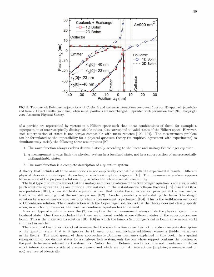
50

FIG. 9. Two-particle Bohmian trajectories with Coulomb and exchange interactions computed from our 1D approach (symbols)and from 2D exact results (solid line) when initial positions are interchanged. Reprinted with permission from [94]. Copyright2007 American Physical Society.

of a particle are represented by vectors in a Hilbert space such that linear combinations of them, for example asuperposition of macroscopically distinguishable states, also correspond to valid states of the Hilbert space. However,such superposition of states is not always compatible with measurements [100, 101]. The measurement problemcan be formulated as the impossibility for a physical quantum theory (in empirical agreement with experiments) tosimultaneously satisfy the following three assumptions [99].

1. The wave function always evolves deterministically according to the linear and unitary Schrodinger equation.

2. A measurement always finds the physical system in a localized state, not in a superposition of macroscopicallydistinguishable states.

3. The wave function is a complete description of a quantum system.

A theory that includes all three assumptions is not empirically compatible with the experimental results. Differentphysical theories are developed depending on which assumption is ignored [16]. The measurement problem appearsbecause none of the proposed solutions fully satisfies the whole scientific community.

The first type of solutions argues that the unitary and linear evolution of the Schrodinger equation is not always valid(such solutions ignore the (1) assumption). For instance, in the instantaneous collapse theories [102] (like the GRWinterpretation [103]), a new stochastic equation is used that breaks the superposition principle at the macroscopiclevel, while still keeping it at the microscopic one [102]. Another possibility is substituting the linear Schrodingerequation by a non-linear collapse law only when a measurement is performed [104]. This is the well-known orthodoxor Copenhagen solution. The dissatisfaction with the Copenhagen solution is that the theory does not clearly specifywhen, in which circumstances, the linear or non-linear equation has to be used.

A second type of solution ignores the (2) assumption that a measurement always finds the physical system in alocalized state. One then concludes that there are different worlds where different states of the superposition arefound. This is the many worlds solution [105, 106] in which the famous Schrodinger’s cat is found alive in one worldand dead in another.

There is a final kind of solutions that assumes that the wave function alone does not provide a complete descriptionof the quantum state, that is, it ignores the (3) assumption and includes additional elements (hidden variables)in the theory. The most spread of these approaches is Bohmian mechanics explained in this book. In a spatialsuperposition of two disjoint states for a single-particle system, only the one whose support contains the position ofthe particle becomes relevant for the dynamics. Notice that, in Bohmian mechanics, it is not mandatory to definewhich interactions are considered a measurement and which are not. All interactions (implying a measurement ornot) are treated identically.

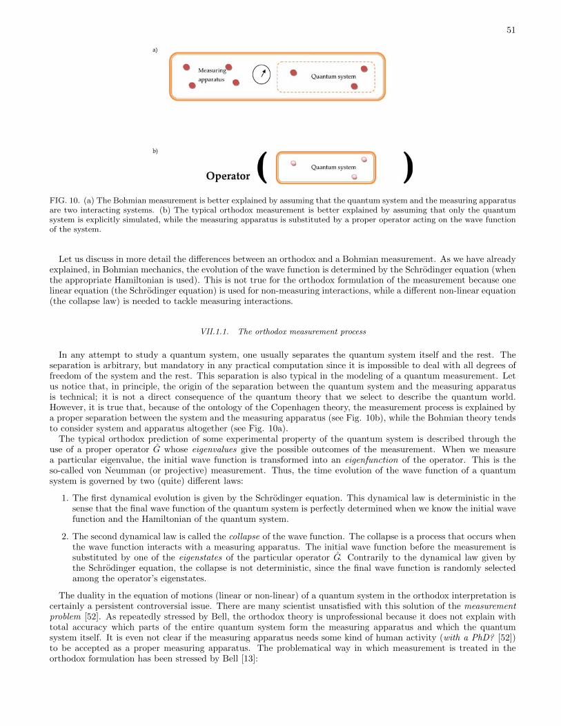
51

FIG. 10. (a) The Bohmian measurement is better explained by assuming that the quantum system and the measuring apparatusare two interacting systems. (b) The typical orthodox measurement is better explained by assuming that only the quantumsystem is explicitly simulated, while the measuring apparatus is substituted by a proper operator acting on the wave functionof the system.

Let us discuss in more detail the differences between an orthodox and a Bohmian measurement. As we have alreadyexplained, in Bohmian mechanics, the evolution of the wave function is determined by the Schrodinger equation (whenthe appropriate Hamiltonian is used). This is not true for the orthodox formulation of the measurement because onelinear equation (the Schrodinger equation) is used for non-measuring interactions, while a different non-linear equation(the collapse law) is needed to tackle measuring interactions.

VII.1.1. The orthodox measurement process

In any attempt to study a quantum system, one usually separates the quantum system itself and the rest. Theseparation is arbitrary, but mandatory in any practical computation since it is impossible to deal with all degrees offreedom of the system and the rest. This separation is also typical in the modeling of a quantum measurement. Letus notice that, in principle, the origin of the separation between the quantum system and the measuring apparatusis technical; it is not a direct consequence of the quantum theory that we select to describe the quantum world.However, it is true that, because of the ontology of the Copenhagen theory, the measurement process is explained bya proper separation between the system and the measuring apparatus (see Fig. 10b), while the Bohmian theory tendsto consider system and apparatus altogether (see Fig. 10a).

The typical orthodox prediction of some experimental property of the quantum system is described through theuse of a proper operator G whose eigenvalues give the possible outcomes of the measurement. When we measurea particular eigenvalue, the initial wave function is transformed into an eigenfunction of the operator. This is theso-called von Neumman (or projective) measurement. Thus, the time evolution of the wave function of a quantumsystem is governed by two (quite) different laws:

1. The first dynamical evolution is given by the Schrodinger equation. This dynamical law is deterministic in thesense that the final wave function of the quantum system is perfectly determined when we know the initial wavefunction and the Hamiltonian of the quantum system.

2. The second dynamical law is called the collapse of the wave function. The collapse is a process that occurs whenthe wave function interacts with a measuring apparatus. The initial wave function before the measurement issubstituted by one of the eigenstates of the particular operator G. Contrarily to the dynamical law given bythe Schrodinger equation, the collapse is not deterministic, since the final wave function is randomly selectedamong the operator’s eigenstates.

The duality in the equation of motions (linear or non-linear) of a quantum system in the orthodox interpretation iscertainly a persistent controversial issue. There are many scientist unsatisfied with this solution of the measurementproblem [52]. As repeatedly stressed by Bell, the orthodox theory is unprofessional because it does not explain withtotal accuracy which parts of the entire quantum system form the measuring apparatus and which the quantumsystem itself. It is even not clear if the measuring apparatus needs some kind of human activity (with a PhD? [52])to be accepted as a proper measuring apparatus. The problematical way in which measurement is treated in theorthodox formulation has been stressed by Bell [13]:

52

The concept of “measurement” becomes so fuzzy on reflection that it is quite surprising to have it appearingin physical theory at the most fundamental level. Less surprising perhaps is that mathematicians, whoneed only simple axioms about otherwise undefined objects, have been able to write extensive works onquantum measurement theory-which experimental physicists do not find it necessary to read. [. . . ] Doesnot any analysis of measurement require concepts more fundamental than measurement? And should notthe fundamental theory be about these more fundamental concepts?

In short, Bell argued that the separation between the quantum system and the measuring apparatus in Fig. 10b isarbitrary. For practical computations, the encapsulation of the rest of the world (except the quantum system) into

a mathematical entity called an operator, G, is a very clever trick that allows for straightforward calculations of theresults of quantum measurements [107, 108] without considering the rest of the world. However, conceptually, the

role played by the operator G as a fundamental part of the orthodox theory is at the origin of the criticism againstthe orthodox solution of the measurement problem.

The reader can argue that, since we have said that the separation between the system and the rest is alwaysarbitrary, one can always enlarge what we consider as a system (see Fig. 10a) also in the orthodox formulation of themeasurement. This would not solve the measurement problem in the orthodox formulation. Certainly, we can enlargethe system in the orthodox quantum formulation of the measurement process by including as a system part of whatwas defined previously as an apparatus. The degrees of freedom of the new system will interact with the degrees offreedom of the old system through a linear equation of motion (Schrodinger equation). Therefore, we will always need

something external to the enlarged system (some new operator G) to provide the collapse of the wave function of theenlarged system.

VII.1.2. The Bohmian measurement process

In Bohmian theory, the measurement process is treated just as any other quantum process of interacting particlesand the previous measurement difficulties of the orthodox interpretation simply disappear. At least, from a conceptualpoint of view. There is no need to introduce operators [72–74, 107, 108]. Here, the entire quantum system is describedby a many-particle trajectory plus a many-particle wave function (rather than a wave function alone). The wavefunction and the trajectory are both associated with the entire system, that is, the quantum system plus the measuringapparatus. Then, there is one dynamical law for the evolution of the wave function and another for the evolution ofthe trajectory:

1. The Schrodinger equation (with the appropriate Hamiltonian of the quantum system plus the measuring ap-paratus) determines the time evolution of the wave function independently of whether a measurement processtakes place or not.

2. The time evolution of the particle is determined by the time integration of the Bohmian velocity independentlyof whether a measurement process takes place or not.

For example, imagine that some kind of pointer indicates the measured quantity; then, the particles (degrees offreedom) that form the pointer must be present in the Hamiltonian.36 In this sense, in Bohmian mechanics, a physicalquantum system must be described by a many-particle Hamiltonian. Once the Bohmian trajectories associated withthe positions of the pointer are known, the value of the measurement is already predicted. We just need knowledgeof the positions of the pointer particles. Again, Bell provided us with one of his didactic sentences [13]:

In physics the only observations we must consider are position observations, if only the positions ofinstrument pointers. It is a great merit of the de Broglie–Bohm picture to force us to consider this fact. Ifyou make axioms, rather than definitions and theorems, about the “measurement” of anything else, thenyou commit redundancy and risk inconsistency.

Therefore, a proper modeling of a Bohmian measurement just needs the explicit consideration of the degrees offreedom of the pointer in the many-particle wave function and many-particle Bohmian trajectories that define theentire system. See Fig. 11. In particular, we have to introduce into the Hamiltonian the interaction of the particlesof the pointer with the rest of the particles of the system. The back reaction of the measurement process on thewave function is trivially considered. Certainly, a Hamiltonian with or without the measuring apparatus will providea different evolution of the quantum system wave function. For this reason, Bell preferred the word “experiment”instead of “measurement.”

36 In modern electronic measuring devices, the pointer could be represented by a seven-segment array of light-emitting diode (LED)displays, each one with two possible states, ON and OFF. When electrons are present inside the PN interface of one of the LEDs, aradiative transition of the electrons from the conduction to the valence band produces light corresponding to the ON state. The absenceof electrons is associated with an OFF state.

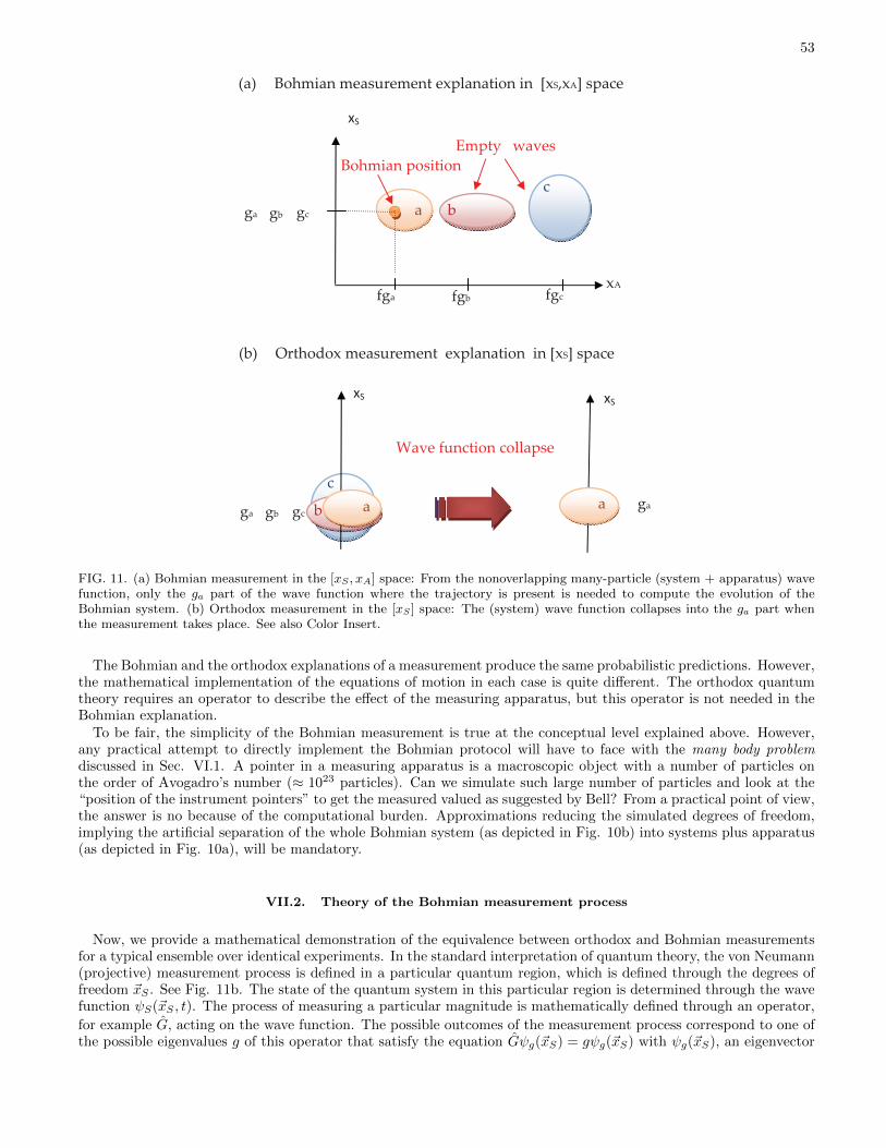
53

Empty waves

Wave function collapse

xA

(a) Bohmian measurement explanation in [xS,xA] space

fga fgb fgc

(b) Orthodox measurement explanation in [xS] space

ga gb gc ga

xS

ga gb gc a b c

a a b

c

xS

xS

Bohmian position

FIG. 11. (a) Bohmian measurement in the [xS , xA] space: From the nonoverlapping many-particle (system + apparatus) wavefunction, only the ga part of the wave function where the trajectory is present is needed to compute the evolution of theBohmian system. (b) Orthodox measurement in the [xS ] space: The (system) wave function collapses into the ga part whenthe measurement takes place. See also Color Insert.

The Bohmian and the orthodox explanations of a measurement produce the same probabilistic predictions. However,the mathematical implementation of the equations of motion in each case is quite different. The orthodox quantumtheory requires an operator to describe the effect of the measuring apparatus, but this operator is not needed in theBohmian explanation.

To be fair, the simplicity of the Bohmian measurement is true at the conceptual level explained above. However,any practical attempt to directly implement the Bohmian protocol will have to face with the many body problemdiscussed in Sec. VI.1. A pointer in a measuring apparatus is a macroscopic object with a number of particles onthe order of Avogadro’s number (≈ 1023 particles). Can we simulate such large number of particles and look at the“position of the instrument pointers” to get the measured valued as suggested by Bell? From a practical point of view,the answer is no because of the computational burden. Approximations reducing the simulated degrees of freedom,implying the artificial separation of the whole Bohmian system (as depicted in Fig. 10b) into systems plus apparatus(as depicted in Fig. 10a), will be mandatory.

VII.2. Theory of the Bohmian measurement process

Now, we provide a mathematical demonstration of the equivalence between orthodox and Bohmian measurementsfor a typical ensemble over identical experiments. In the standard interpretation of quantum theory, the von Neumann(projective) measurement process is defined in a particular quantum region, which is defined through the degrees offreedom ~xS . See Fig. 11b. The state of the quantum system in this particular region is determined through the wavefunction ψS(~xS , t). The process of measuring a particular magnitude is mathematically defined through an operator,

for example G, acting on the wave function. The possible outcomes of the measurement process correspond to one ofthe possible eigenvalues g of this operator that satisfy the equation Gψg(~xS) = gψg(~xS) with ψg(~xS), an eigenvector

54

of this operator. The set ψg(~xS) forms an orthonormal basis of the Hilbert space of the quantum system so that thearbitrary initial wave function can be written as:

ψS(~xS , t) =∑g

cg(t)ψg(~xS) (113)

with cg(t) =∫ψS(~xS , t)ψ

∗g(~xS) a complex value with the only restriction

∑g |cg(t)|2 = 1 in order to ensure that

ψS(~xS , t) is well normalized. When measuring the eigenvalue ga the total wave function ψS(~xS , t) collapses intoψga(~xS). Then, the probability of obtaining ga in the measuring apparatus is just Pga = |cga(t)|2. To avoid unnecessarycomplications, hereafter, we have assumed that the basis ψg(~xS) has no degeneracy.

In order to understand how this (von Neumann) measurement can be described by means of Bohmian mechanics,we use the Schrodinger equation plus a trajectory, defined both in the enlarged configuration space that includes thequantum system and the measuring apparatus. There is no privileged status for the observer, that is, the measuringapparatus, over the quantum system. This is the reason why some authors describe Bohmian theory under the titleof “quantum mechanics without observers” [96].

Surprisingly, this idea was, somehow, anticipated in the book Quantum Theory, published in 1951 [39], by Bohm.Although in this book Bohm followed an orthodox presentation of quantum mechanics, he also provided a detailed andconceptually intricate treatment of the measurement process in chapter 22. First, Bohm demanded in unequivocalterms a quantum theoretical treatment of the entire process of measurement within the Schrodinger equation. Inparticular, he argued that a good measuring apparatus will force the wave function to decouple into several nonover-lapping wave packets. Each one of these wave packets can be associated to one particular value of the measurementprocess. Second, he supplemented his measurement process by adding some obscure discussion about decoherencewhere only one of the several wave packets survives (as we mentioned at the end of Sec. VII.1.1, even after enlargingthe system, one has to invoke somehow the collapse of the wave function). After 1951, when Bohm presented his“hidden variables” theory [8, 9], he kept the first part of his previous explanation of the measurement process andthen provided a simple explanation about the final selection of the available wave packets: the selected wave packetis the one that contains the trajectory,37 see Fig. 1.10(a).

Our mathematical demonstration on how Bohmian mechanics explains the (von Neumann) measurement follows[24, 72, 74, 95, 107]. In order to be able to define the measurement process in the Bohmian formalism, apart from thedegrees of freedom ~xS , we need the degrees of freedom of the positions ~xA of the pointer belonging to a measuringapparatus.38 Thus, we define a total wave function ΦT (~xS , ~xA, t) in a larger configuration space that includes thequantum region plus the measuring region, ~xS , ~xA. According to the Bohmian postulates, we do also select atrajectory ~xS [t], ~xA[t] in this larger configuration space. The (Bohmian) time evolution of the total wave functionand the total trajectory is what we need to explain the (von Neumann) measurement process described earlier .

There are some necessary conditions that the time-evolution of the entire Bohmian system has to satisfy to saythat a measuring apparatus is able to correctly determine the eigenvalues g. First, the pointer positions ~xA[t] of suchan apparatus have to be restricted to a particular region, ~xA[t] ∈ Sg1 , every time that the quantum system is inthe eigenstate ψg1

(~xS). Let us define Φg1(~xS , ~xA, t) as the total wave function that fits with the property that any

experiment whose quantum system is described by ψg1(~xS) implies that the pointer points in the particular region,

~xA[t] ∈ Sg1. A second necessary condition for a good measuring apparatus of the eigenvalue g is that Sg1 ∩ Sg2 = 0

when we measure. We have defined the restricted region allowed by the pointer positions associated with a secondeigenstate, ψg2

(~xS), as ~xA[t] ∈ Sg2. This implies that the states Φg1

(~xS , ~xA, t) and Φg2(~xS , ~xA, t) do not overlap in

the larger configuration space during the measurement.Since the eigenstates ψg(~xS) form a complete basis, we can decomposed any function, and in particular each

Φg(~xS , ~xA, t), into the following sum:

Φg(~xS , ~xA, t) =∑g′

fg′(~xA, t) ψg′(~xS), (114)

with fg(~xA, t) =∫

Φg(~xS , ~xA, t)ψ∗g(~xS)d~xS . However, from our previous discussion about the properties of a “good”

von Neumann measurement apparatus, Φg(~xS , ~xA, t) cannot be a sum over different eigenstates ψg(~xS) in Eq. (114)because then the measuring apparatus would provide the same pointer position ~xA[t] ∈ Sg for different eigenstates.Thus, during the time of the measurement, the only good decomposition for Φg(~xS , ~xA, t) is:

Φg(~xS , ~xA, t) = fg(~xA, t) ψg(~xS) (115)

37 Very roughly speaking, Bohmian mechanics avoids the need to select randomly the final wave packet because the initial position of thetrajectory has already selected the final wave packet at the beginning.

38 In fact, we would have to include all others degrees of freedom of the “environment,” ~xE , needed to be able to assume that the consideredentire system is a closed one described by a pure (not mixed) state. In addition, as mentioned in Sec. VII.1.2, we emphasize that apointer in a measuring apparatus is a macroscopic object with a number of particles on the order of Avogadro’s number, not the singledegree of freedom ~xA[t] used here. A single degree of freedom cannot be considered a pointer because it is not a macroscopic object(we do not see ~xA[t]). In any case and without loss of generality, we perform here a conceptual demonstration with a single degree offreedom ~xA[t] for the pointer.

55

We emphasize that fg(~xA, t) is a normalized function because Φg(~xS , ~xA, t) and ψg(~xS) are also normalized functionsin their respective configurations spaces. By its own construction, fg1

(~xA, t) ∩ fg2(~xA, t) = 0 during the measuring

time. Thus, even if ψg1(~xS) and ψg2

(~xS) overlap, the states Φg1(~xS , ~xA, t) and Φg1

(~xS , ~xA, t) do not overlap in thelarger configuration space. See Fig. 11a. Thus, we can ensure that a general function in the quantum system, Eq.(113), can be rewritten in the whole, that is, quantum plus measuring, configuration space associated to a goodmeasuring apparatus as:

ΦT (~xS , ~xA, t) =∑g

cg(t) fg(~xA, t) ψg(~xS) (116)

In summary, during the time of measurement, the only total wave functions that can live in the entire quantum systemthat includes a good (in this case a projective or Von-Neumann type) measuring apparatus of the eigenvalues g are theones written in Eq. (116). An example of such wave functions is depicted in Fig. 11a. It is important to notice thatEq. (116) implies no restriction on the wave function ψS(~xS , t) but only on the total wave function ΦT (~xS , ~xA, t). Ifthese restrictions are not respected, we can find other types of total wave functions in the configuration space ~xS , ~xA,but they would be incompatible with stating that we have an apparatus that is able to measure the eigenavalue gwith certainty at time t.

After this discussion, we can show quite trivially how the von Neumann measurement is exactly reproduced withBohmian mechanics. As we have mentioned, apart from the wave function in Eq. (116), we have to select an initialtrajectory ~xS [0], ~xA[0]. Such a trajectory will evolve with the total wave function, and during the measurement,the particle trajectory ~xS [t], ~xA[t] will be situated in only one of the nonoverlapping wave packets of Eq. (116), forexample fga(~xA, t)ψga(~xS) as depicted in Fig. 11a. Thus, the pointer positions will be situated in ~xA[t] ∈ Sga and wewill conclude with certainty that the eigenvalue of the quantum system is ga. In addition, the subsequent evolutionof this trajectory can be computed from fga(~xA, t)ψga(~xS) alone. In other words, we do not need the entire wavefunction Eq. (116) because the particle velocity can be computed from fga(~xA, t)ψga(~xS). The rest of circles of Fig.11a are empty waves that do not overlap with fga(~xA, t)ψga(~xS) so that they have no effect on the velocity of theBohmian particle39. This is the simple explanation of how the complicated orthodox collapse is interpreted withinBohmian mechanics. This discussion is depicted in Fig. 11

We have mentioned before that the von Neumann measurement predicts that the probability of finding ga isPga = |cga(t)|2. We can easily recover this result from our Bohmian picture. This probability is obtained after therepetition of the same experiment, with the same ΦT (~xS , ~xA, t), many times. The second (quantum equilibrium)postulate of Bohmian mechanics (see Sec. VI.5) ensures that the modulus of the wave function will be reproduced bythe trajectories when we repeat the same experiment many times. Then, the probability of finding the eigenvalue ga,that is, the eigenstate ψga(~xS), is just:

Pga =

∫ ∫|cga(t)fga(~xA, t)ψga(~xS)|2d~xSd~xA∫ ∫ ∑g |cg(t)fg(~xA, t)ψg(~xS)|2d~xSd~xA

=|cga(t)|2∑g |cg(t)|2

= |cga(t)|2 (117)

where we have explicitly used the condition that the each Φg1(~xS , ~xA, t) does not overlap with the others for the

computation of the modulus of the total wave function, |ΦT (~xS , ~xA, t)|2, in the denominator. Additionally, we use∫|ψg(~xS)|2d~xS = 1,

∫|fg(~xA, t)|2d~xA = 1, and

∑g |cg(t)|2 = 1. Thus, the same probabilistic predictions are obtained

from Bohmian and orthodox quantum formulations when a von Neumann measurement is performed.We want to enlarge the explanation of the role played by the empty waves belonging to the wave packet of Eq.

(116), which do not contain the particle. In principle, one can argue that such empty waves can evolve and, inlater times, overlap with the original wave that contains the particle. If we are interested in doing subsequent (i.e.,two times) quantum measurements, a good measuring apparatus has to avoid these “spurious” overlaps. This can beunderstood as an additional condition for qualifying our measuring apparatus as a good apparatus. In the examples ofthe subsequent subsections VII.2.1 and VII.2.2, we will realize that the assumption of nonoverlapping between emptyand full waves can be very reasonable in many practical implementations of the measuring apparatus. In fact, in areal system with a very large number of particles associated to the apparatus (or the environment), the probabilitythat such overlap occurs in the configuration space of all the particles is almost null. See a discussion on page 79in Ref. [95]. If the empty wave packets later coincide (by putting some reflected mirrors for example), then, theapparatus described above would not be a good apparatus to measure eigenvalues. On the contrary, this apparatus(with the mirrors) would be a very interesting/enlightening design to test quantum interference effects with waves

39 Let us remind that, in a realistic measuring apparatus, the number of particles of the pointer is around the Avogadro’s number.Therefore, the wave functions fg(~xA, t)ψg(~xS) live in a N = 1023 configuration space where the possibility of a coincidence of twoempty waves is almost zero.

56

and particles. The double-slit experiment is the most famous example of interference effects between empty and fullwave packets.

Finally, let us mention that we have only considered von Neumann (i.e., projective) measurements. Other typesof measurements are also possible, which do not collapse into an eigenstate (for example, the generalized or weakmeasurements). Obviously, such generalized measurements can also be explained within Bohmian mechanics with anextension of the simple ideas for projective measurements discussed here [72, 95, 107].

VII.2.1. Example: Bohmian measurement of the momentum

Let us explain the momentum measurement of the stationary state of an electron initially in an energy eigenstateof a square well of size L. For example, ψn(x) = C sin(nπx/L) within the well and zero elsewhere, C being thenormalization constant and n an integer (denoting the vibrational state). Since the wave function is real, we obtainp = ∂S(x)/∂x = 0. Thus, the Bohmian particle is at rest, meaning that its velocity and kinetic energy are zero.However, we know that for a high enough value of n, the previous wave function ψ(x) can be roughly approximatedby a sum of two momentum eigenstates with eigenvalues ±nh/L. Therefore, when we do a (Copenhagen) momentummeasurement, we will obtain an outcome ±nh/L and the previous wave function will collapse into one of the twomomentum eigenstates.

We have shown that the Bohmian measurement has to provide the same eigenvalues and eigenstates. How? Theanswer is that according to the Bohmian measurement, we have to specify in detail how the measurement processdevelops; which is the Hamiltonian that provokes the measurement.

A measurement of the momentum, for example, can be undertaken by removing the walls that form the well anddetecting the electron somewhere in a screen far from the initial walls. The time interval between removing the wallsand detecting the particles will allow us a computation of the “electron velocity.” The time-dependent process ofremoving the walls will imply that the stationary wave function will evolve into two time-dependent wave packetsmoving on opposite directions, which will become completely separated in space. The particle will end in one wavepacket or the other with a momentum very close to±nh/L, the sign depending on which wave packet the initial positionof the particle enters [9]. Finally, the electron will be detected far from the walls after the appropriate interval of time.For this particular experiment, we are sure that the empty wave will not affect the wave that carries the particle.As mentioned earlier, the relevant point is that we have been able to measure the same eigenstates and eigenvaluespredicted by the orthodox interpretation without invoking the collapse of the wave function as a fundamental law.

In order to understand the Bohmian explanation of this experiment, it is important to discuss the roles played bythe kinetic and quantum potentials. The initial Bohmian kinetic energy is zero, while the initial quantum potentialis Q(x, t) = (nh/L)2/(2m) for the initial state ψ(x) = C sin(nπx/L). On the contrary, the final energy of the systemappears in the form of kinetic energy of electrons (nh/L)2/(2m), while the final quantum potential from Eq. (6) isnegligible Q(x, t) ∼ 0. See problem 10.

The reader will realize that we have not follow all the indications of the previous section. In principle, for a formalBohmian discussion of measurement, we would have to discuss the wave function and particles of the whole quantumplus measuring apparatus system. However, in this section we have avoided the wave function and trajectory relatedto the measuring apparatus. In this example, the screen is the measuring apparatus of the position of the system’sparticle. The part of the measuring process involving the screen has not been explicitly described in our example (wecould obviously explain why a proper coupling of the degrees of freedom of the system and the screen will imply thatafter impinging with the screen, the system wave function becomes a wave packet highly localized around the positionof the measurement, but we have not done it because it is quite obvious).

This example clearly shows that what we get from a measurement depends on the measurement itself. We haveexplained an experiment to measure the velocity of the particle. In fact, the Bohmian particle was at rest (with zerovelocity) before we start the measurement. However, because of the type of measurement that we have designed, theBohmian particle acquires a non-zero velocity. What we get from the measurement is exactly this non-zero value ofthe velocity, but this is not the pre-existing velocity of the particle before the measurement. Contrarily to a classicalmeasurement, in the quantum world, in general, we cannot get information of a quantum system from a measurementwithout providing some type of perturbation on it. This property of quantum phenomena is named contextuality.

VII.2.2. Example: Sequential Bohmian measurement of the transmitted and reflected particles

We provide another didactic example of how Bohmian mechanics explains sequential measurements. The wavepackets in Fig. 12 represent the solution of the (unitary) Schrodinger equation for a wave packet incident upona tunneling barrier, at three different times. The initial wave packet (with norm equal to one) is divided into atransmitted plus a reflected wave packet. According to the Copenhagen interpretation, when the system is measured

57

FIG. 12. Schematic explanation of the ability of Bohmian mechanics to discuss the unitary and nonunitary evolution of a wavepacket incident upon a tunneling barrier for three different times t0 < t1 < t2.

at time t1, a nonunitary evolution appears in the wave function. Thus, randomly, for example the reflected wavepacket disappears. Only the transmitted wave packet describes the electron at time t1. Then, when the system ismeasured again at t2, the electron is only represented by the transmitted wave packet.

Alternatively, the same evolution can be explained with Bohmian mechanics. The initial position of the Bohmiantrajectory is selected according to the quantum equilibrium hypothesis at the initial time t0. Let us assume thatwe select an initial position that corresponds to a trajectory that is finally transmitted. Then, at times t1 and t2,the evolution of the trajectory is only determined by the transmitted wave packet because the reflected wave packetis an “empty wave” that has no effect on the evolution of the trajectory. Here, we have implicitly assumed thatthe eigenstates of the measuring apparatus are transmitted wave packets for positive currents, and reflected ones fornegative currents.

As expected, the probability of measuring, first, the particle as being transmitted at time t1 and measuring, after,the same particle as being reflected at time t2 is zero either with orthodox or Bohmian mechanics.

Again, the reader can argue that we have not enlarged the system including the measuring apparatus. Next, weprovide a more formal description of the Bohmian measurement of the charge for a tunneling electron includingthe quantum system plus the measuring apparatus. The quantum system is defined by an electron labeled as x1[t]impinging on a tunneling barrier. Behind the barrier there is a measuring device named the “transmitted chargedetector” and modeled as a single degree of freedom x2[t], which can detect the successful transmission of an electron.The dynamic of the system plus apparatus includes, first, an interaction of the electron with the potential barrier and,subsequently, an interaction with the transmitted charge detector. It is important to stress that both interactions areregarded at the very same level within Bohmian mechanics. The measurement interaction introduces a channelizationof the wave function in the configuration space such that the desired property of the quantum system (here, whetherthe electron is reflected or transmitted) can be read off from the final position x2[t] of a particle, which plays the roleof the pointer of the apparatus. The interaction between the electron and the pointer can be modeled as:

Hint = λQ(x1)Px2 = −ihλQ(x1)∂

∂x2, (118)

where Px2= −ih∂/∂x2 is the momentum operator of the detector and λ = 50 nm/ps is the interaction constant.

Q(x1) is a function that is equal to zero when the electron is outside the detector, (x1 < 75 nm in Fig. 13), andis equal to one when the particle is inside the detector (x1 > 75 nm).40 In Fig. 13 the region in the configurationspace in which Q(x1) is different from zero is represented by a rectangle in the right of the figure. The many-particleSchrodinger equation reads

ih∂Ψ(x1, x2, t)

∂t=(− h2

2m

∂2

∂x21

− h2

2M

∂2

∂x22

+ U(x1)− ihλQ(x1)∂

∂x2

)Ψ(x1, x2, t),

(119)

where m is the effective mass of the electron, M is the mass of the apparatus pointer and U(x1) is the externalpotential energy barrier seen as a vertical line in the middled of Fig. 13.

40 The transition of Q(x1), from zero to one, is softly done in order to minimize the perturbation of the quantum system as explained inRef. [109, 110].

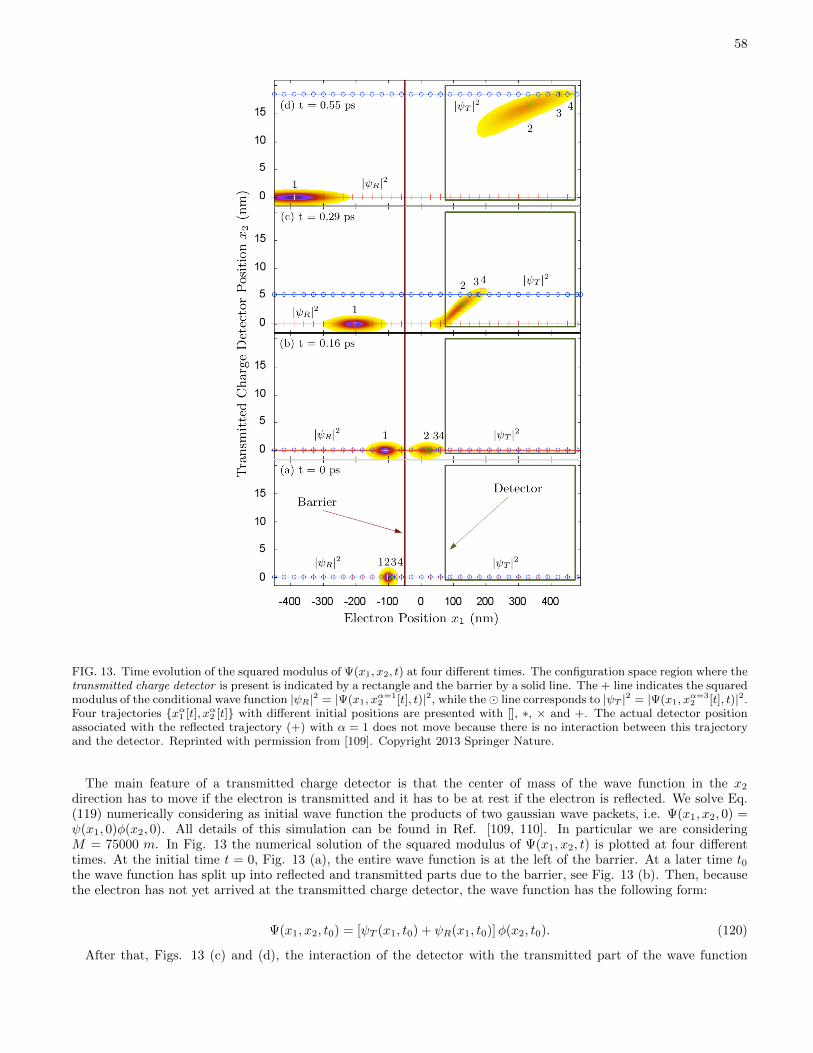
58

FIG. 13. Time evolution of the squared modulus of Ψ(x1, x2, t) at four different times. The configuration space region where thetransmitted charge detector is present is indicated by a rectangle and the barrier by a solid line. The + line indicates the squaredmodulus of the conditional wave function |ψR|2 = |Ψ(x1, x

α=12 [t], t)|2, while the line corresponds to |ψT |2 = |Ψ(x1, x

α=32 [t], t)|2.

Four trajectories xα1 [t], xα2 [t] with different initial positions are presented with [], ∗, × and +. The actual detector positionassociated with the reflected trajectory (+) with α = 1 does not move because there is no interaction between this trajectoryand the detector. Reprinted with permission from [109]. Copyright 2013 Springer Nature.

The main feature of a transmitted charge detector is that the center of mass of the wave function in the x2

direction has to move if the electron is transmitted and it has to be at rest if the electron is reflected. We solve Eq.(119) numerically considering as initial wave function the products of two gaussian wave packets, i.e. Ψ(x1, x2, 0) =ψ(x1, 0)φ(x2, 0). All details of this simulation can be found in Ref. [109, 110]. In particular we are consideringM = 75000 m. In Fig. 13 the numerical solution of the squared modulus of Ψ(x1, x2, t) is plotted at four differenttimes. At the initial time t = 0, Fig. 13 (a), the entire wave function is at the left of the barrier. At a later time t0the wave function has split up into reflected and transmitted parts due to the barrier, see Fig. 13 (b). Then, becausethe electron has not yet arrived at the transmitted charge detector, the wave function has the following form:

Ψ(x1, x2, t0) = [ψT (x1, t0) + ψR(x1, t0)]φ(x2, t0). (120)

After that, Figs. 13 (c) and (d), the interaction of the detector with the transmitted part of the wave function

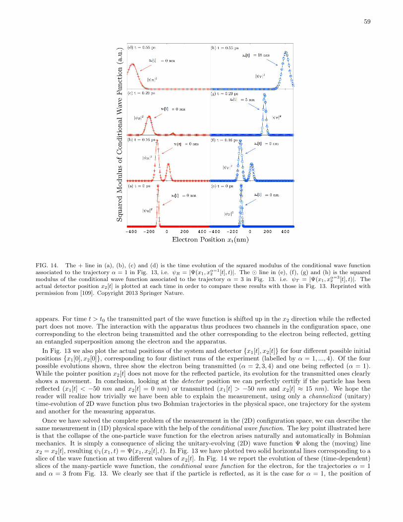
59

FIG. 14. The + line in (a), (b), (c) and (d) is the time evolution of the squared modulus of the conditional wave functionassociated to the trajectory α = 1 in Fig. 13, i.e. ψR = |Ψ(x1, x

α=12 [t], t)|. The line in (e), (f), (g) and (h) is the squared

modulus of the conditional wave function associated to the trajectory α = 3 in Fig. 13. i.e. ψT = |Ψ(x1, xα=32 [t], t)|. The

actual detector position x2[t] is plotted at each time in order to compare these results with those in Fig. 13. Reprinted withpermission from [109]. Copyright 2013 Springer Nature.

appears. For time t > t0 the transmitted part of the wave function is shifted up in the x2 direction while the reflectedpart does not move. The interaction with the apparatus thus produces two channels in the configuration space, onecorresponding to the electron being transmitted and the other corresponding to the electron being reflected, gettingan entangled superposition among the electron and the apparatus.

In Fig. 13 we also plot the actual positions of the system and detector x1[t], x2[t] for four different possible initialpositions x1[0], x2[0], corresponding to four distinct runs of the experiment (labelled by α = 1, ..., 4). Of the fourpossible evolutions shown, three show the electron being transmitted (α = 2, 3, 4) and one being reflected (α = 1).While the pointer position x2[t] does not move for the reflected particle, its evolution for the transmitted ones clearlyshows a movement. In conclusion, looking at the detector position we can perfectly certify if the particle has beenreflected (x1[t] < −50 nm and x2[t] = 0 nm) or transmitted (x1[t] > −50 nm and x2[t] ≈ 15 nm). We hope thereader will realize how trivially we have been able to explain the measurement, using only a channelized (unitary)time-evolution of 2D wave function plus two Bohmian trajectories in the physical space, one trajectory for the systemand another for the measuring apparatus.

Once we have solved the complete problem of the measurement in the (2D) configuration space, we can describe thesame measurement in (1D) physical space with the help of the conditional wave function. The key point illustrated hereis that the collapse of the one-particle wave function for the electron arises naturally and automatically in Bohmianmechanics. It is simply a consequence of slicing the unitary-evolving (2D) wave function Ψ along the (moving) linex2 = x2[t], resulting ψ1(x1, t) = Ψ(x1, x2[t], t). In Fig. 13 we have plotted two solid horizontal lines corresponding to aslice of the wave function at two different values of x2[t]. In Fig. 14 we report the evolution of these (time-dependent)slices of the many-particle wave function, the conditional wave function for the electron, for the trajectories α = 1and α = 3 from Fig. 13. We clearly see that if the particle is reflected, as it is the case for α = 1, the position of

60

the pointer does not change with time and, after the interaction with the detector has been performed, the electron’sconditional wave function includes only a reflected part. See Figs. 14 (c) and (d). On the other hand, when theparticle is transmitted (e.g., α = 3), it is the reflected part of the conditional wave function which collapses away,leaving only the transmitted packet. See Figs. 14 (g) and (h). Note that the evolution of ψ1(x1, t) (the electron’sconditional wave function) is not unitary, even though the evolution of Ψ is.

While a wave function formulation of quantum mechanics provides only statistical information about the experi-mental results, with the help of the Bohmian trajectories, we have been able to recover the individual result of eachexperiment. In fact for each experiment the pointer of the detector is either moving (corresponding to a transmittedelectron) or not (reflected electron), while an ensemble of repeated experiments (where the initial positions of theparticles, both the electron x1[0] and the detector x2[0], are selected according to the squared modulus of the wavefunction at the initial time |Ψ(x1, x2, 0)|2) reproduce the same statistical results.

Finally, by looking at figures 13 and 14, we conclude that the Bohmian theory provides a quite simple explanationon when, why and how the (conditional) wave function collapses. The Bohmian explanation of the measurement,with waves and particles, demystifies the orthodox postulate of the collapse law by explaining it as a trivial result ofmaking a transition from a large configuration space (quantum system plus apparatus) to a smaller one (quantumsystem alone). To be fair, in spite of its extraordinary simplicity to explain the collapse law, the model explainedhere for measuring the transmitted charge has still an important approximation. We have assumed that the pointeris just one degree of freedom x2[t]. As we have already mentioned, a realistic model for the pointer has to involve avery large number of particles (on the order of Avogadro’s number ≈ 1023). Then, we will also be able to concludethat the macroscopic pointer has a classical behavior. However, such type of simulation involves facing again withthe many body problem mentioned in Sec. VI.1. Some preliminary discussions on the classical-quantum transitionfor macroscopic objects can be found in Refs. [67, 111–114].

VII.3. The evaluation of a mean value in terms of Hermitian operators

VII.3.1. Why Hermitian operators in Bohmian mechanics?

In the previous section, we have emphasized the ability of Bohmian mechanics to address quantum phenomenajust from the Schrodinger equation and the equation of motion of the trajectories. The operators, which are anindispensable tool in the orthodox formulation of quantum mechanics to deal with the measurement process, becomeunnecessary in the Bohmian formulation. Once one realizes that operators are unnecessary, the conceptual difficultiesassociated with the wave function collapse of the orthodox formulation disappear (as we have seen in passing fromFig. 13 to Fig. 14). However, we have mentioned that the Bohmian measurement process explained above (withan idealized single-particle pointer) has limited practical utility. Including the measuring apparatus into the entireHamiltonian is not an easy task, because it implies increasing the number of degrees of freedom. The exact Bohmiansimulation of the measurement process is, most of the time, a quite difficult computational task.

In these circumstances, the use of a Hermitian operator acting only on the wave function of the quantum systemwith the ability of providing the outcomes of the measurement process without the explicit simulation of the measuringapparatus is very welcomed. Let us emphasize that we are talking only at the computational level. In simple words,operators are not needed in Bohmian mechanics (the operators are part of the Copenhagen ontology, but they are notpart of the Bohmian ontology), but they are a very helpful mathematical trick in practical computational issues. Theseideas are emphasized by Goldstein, Durr, Teufel, and coworkers when they refer to the “naive realism about operators”[72, 107, 108]. Somehow, we are arguing here that the Copenhagen theory can be transformed into an effective modelof the Bohmian theory where trajectories are deliberatively ignored for computational/practical proposals. Then,although we have a computational ignorance about the position of such electron, the idea of an (unmeasured) electrontraversing a tunneling barrier would be fully supported by such effective quantum theory.

VII.3.2. Mean value from the list of outcomes and their probabilities

We now want to reproduce the mean value, obtained from orthodox Hermitian operators, within Bohmian mechan-ics. Someone who dislikes what we have explained up to here about the Bohmian measurement can just focus onhow Bohmian trajectories exactly reproduce the mean value of orthodox Hermitian operators. For simplicity, we willconsider single-particle systems. The generalization to many-particle systems can be done straightforwardly.

First, according to the orthodox measurement, we assume that a particular experiment is described by the quantumsystem wave function ψ(x, t) alone. After a large number, M , of repetitions of the same experiment, we can elaborate

61

a large list i = 1 . . . , I of the possible outcomes ai with their occurrence probabilities Pi. From this data we cancompute the mean value as: ⟨

A⟩ψ

=

I∑i=1

aiPi (121)

This is the standard (classical or quantum) definition of the mean value.

VII.3.3. Mean value from the wave function and the operators

According to the orthodox quantum theory, an observable is associated with a Hermitian operator A that describesthe measurement process. Such an operator fulfills A|ui〉 = ai|ui〉, |ui〉 being its eigenstates. Therefore, Pi =〈ψ|ui〉〈ui|ψ〉 so that we can write:

⟨A⟩ψ

= 〈ψ|

(I∑i=1

ai|ui〉〈ui|

)|ψ〉 =

⟨ψ∣∣∣ A ∣∣∣ψ⟩ (122)

where we have used ai|ui〉 = A|ui〉 and we have identified the expression∑Ii=1 |ui〉〈ui| as the identity because of the

orthonormality of the eigenstates. Therefore, we can compute the mean value of an ensemble of experiments from Eq.(122) by only knowing the wave function and the operator (without knowing either the eigenstates or the outcomevalues and their probabilities). Thus, we have been able to compute mean values within the orthodox quantuminterpretation without directly mentioning the wave function collapse.

VII.3.4. Mean value from Bohmian mechanics in the position representation

We can always write the Hermitian operator A and the mean value⟨A⟩ψ

in the position representation. Then, the

mean value of this operator over the wave function ψ(x, t) is given by:⟨A⟩ψ

=

∫ ∞−∞

ψ∗(x, t)A

(x,−ih ∂

∂x

)ψ(x, t)dx (123)

Alternatively, the same mean value can be computed from Bohmian mechanics by defining a spatial average of a“local” magnitude AB(x) weighted by R2(x, t):⟨

A⟩ψ

=

∫ ∞−∞

R2(x, t)AB(x)dx (124)

In order to obtain the same value with Eqs. (123) and (124), we can easily identify the local mean value AB(x) as:

AB(x) = Real

[ψ∗(x, t)A (x,−ih ∂∂x

)ψ(x, t)

ψ∗(x, t)ψ(x, t)

]ψ(x,t)=R(x,t)ei

S(x,t)h

(125)

We take only the real part, Real(), because we know that the mean value must be real, and Eq. (125) without Real()could take complex values.

VII.3.5. Mean value from Bohmian trajectories

For practical purposes, we will compute the mean value using Eq. (124) with a large j = 1, . . . ,M numberof Bohmian trajectories with different initial positions. We will select the initial position xj [t0] of the Bohmiantrajectories according to the second postulate. Therefore, we can use Eq. (50) to write R2(x, t) in Eq. (124). Finally,we obtain: ⟨

A⟩ψ

= limM→∞

1

M

M∑j=1

AB(xj [t]). (126)

62

By construction, in the limit M →∞, the value of Eq. (126) is identical to the value of Eq. (124).Now, we provide several examples of how some common mean values are computed from the orthodox quantum

formalism and from Bohmian trajectories. First, we compute the mean value of the position:

〈x〉ψ =

∫ ∞−∞

ψ∗(x, t)xψ(x, t)dx (127)

with xB(x) = x so that:

〈x〉ψ =

∫ ∞−∞

R2(x, t)xdx (128)

Identically, the mean value of the momentum:

〈p〉ψ =

∫ ∞−∞

ψ∗(x, t)

(−ih ∂

∂x

)ψ(x, t)dx (129)

with pB(x) = ∂S(x, t)/∂x:

〈p〉ψ =

∫ ∞−∞

R2(x, t)∂S(x, t)

∂xdx (130)

For the classical potential, we have:

〈V 〉ψ =

∫ ∞−∞

ψ∗(x, t)V (x, t)ψ(x, t)dx (131)

with VB(x, t) = V (x, t) so that:

〈V 〉ψ =

∫ ∞−∞

R2(x, t)V (x, t)dx (132)

Now, we compute the mean value of the kinetic energy:

〈K〉ψ =

∫ ∞−∞

ψ∗(x, t)

(− h2

2m

∂2

∂x2

)ψ(x, t)dx (133)

It is important to notice that the local mean value of the kinetic energy takes into account the Bohmian kinetic energyplus the quantum potential. In particular, KB(x) can be obtained from the expression:

KB(x) = Real

(−R(x, t)e−iS(x,t)/h h2

2m

(∂∂x

)2R(x, t)eiS(x,t)/h

R2(x, t)

)(134)

The real part41 of KB is:

KB =1

2m

(∂S(x, t)

∂x

)2

+Q(x, t) (135)

so that, finally, we obtain the Bohmian expression of the mean kinetic energy of the ensemble of trajectories:

〈K〉ψ =

∫ ∞−∞

R2(x, t)

(1

2m

(∂S(x, t)

∂x

)2

+Q(x, t)

)dx (136)

See problem 10 for a detailed calculation and the explanation of the meaning of the two terms.

41 It can be demonstrated quite easily that the imaginary part of Eq. (134) is equal to the spatial derivative of the current that becomeszero when integrated over all space. We use J(x = ±∞, t) = 0, which is always valid for wave functions that are normalized to unity,but it is not true for other types of wave functions such as plane waves.

63

Finally, we compute the mean value of the current density operator. First, let us remark that the probabilitydensity operator can be written as |x〉〈x| and its expected mean value is 〈ψ|x〉〈x|ψ〉 = |ψ(x, t)|2 or, in the Bohmian

language, 〈ψ|x〉〈x|ψ〉 = R2(x, t). The (Hermitian) current operator can be written as J = 1/(2m)(|x〉〈x|p+ p|x〉〈x|).It can be easily demonstrated that:

〈J〉ψ = J(x, t) = v(x, t)R2(x, t) = limM→∞

1

M

M∑j=1

v(xj [t])δ(x− xj [t]). (137)

The average value of the current density depends on the position, and it is equal to the average Bohmian velocitymultiplied by the squared modulus of R(x, t). At a particular position “x,” this current is just the sum of all particlesthat reside arround this position x = xj [t] at time t, multiplied by the Bohmian velocity at such position and time.

VII.3.6. On the meaning of local Bohmian operators AB(x)

It is important to emphasize that the local Bohmian operators AB(x) are not the eigenvalues of the operator A.In general, the eigenvalues are not position dependent, while AB(x) are. The expression AB(x) is what is needed

to compute the mean values of A with Eq. (124). This is its exact meaning. We have encapsulated all the effectsof the measuring apparatus on the system into AB(x). Somehow, the use of AB(x) seems to emphasize that we aremeasuring a pre-existent property of the system, while we have learnt during this section devoted to the measurementthat an interaction between system and apparatus during the time taken for doing the measurement (see Fig. 13) ismandatory.

There is a well-known example, mentioned in the previous Sec. VII.2.1, that emphasizes the differences betweeneigenvalues and local Bohmian operators. We consider the particle between two walls, separated by a distance L,whose wave function is ψ(x) = C sin(nπx/L) within the walls and zero elsewhere. Since the wave function is real, weobtain p = ∂S(x)/∂x = 0. Thus, the local Bohmian momentum is pB(x) = ∂S(x, t)/∂x = 0, and the mean value inEq. (130) is also zero. On the contrary, the wave function can be written as:

ψ(x) ≈ C ′(e−iπx/L − eiπx/L

)(138)

We know that ei nπx/L and e−i nπx/L are eigenstates of the momentum operator with eigenvalues a1 = nhπ/L anda2 = −nhπ/L, respectively. Thus, the probabilities for each of these eigenvalues are identical, and the mean value ofthe momentum from Eq. (121) is again zero.

In conclusion, in general, AB(x) cannot be identified with ai. However, by construction, the mean values computedfrom ai and AB(x) are identical. A similar discussion about the evaluation of the mean value of the quantum powercan be found in Ref. [115].

In this Sec. VII.3, we have only discussed how the mean values (i.e., the first moment) obtained from orthodoxquantum mechanics can be exactly reproduced within Bohmian mechanics. More complicated higher moments (e.g.,the second moment called the variance, whose positive square root is the standard deviation) computed from orthodoxquantum mechanics can be equivalently reproduced within Bohmian mechanics, as we anticipated in Sec. VII.2.2[72, 107, 108]. With the appropriate care on the contextuality of quantum phenomena, two-time correlations functionscan also be computed in the same way. See also Ref. [116].

VIII. CONCLUDING REMARKS

In this chapter we have provided a fully comprehensive and didactic overview of the Bohmian formulation ofquantum mechanics that can be useful for understanding the following chapters and also for any newcomers interestedin using Bohmian mechanics in their daily research activity.

To be fair, most of the research on quantum phenomena is developed with the orthodox machinery, and few signi-ficative contributions have been performed with Bohmian mechanics. Many researchers ignore Bohmian mechanics,or they decide not to use it because they believe that someone demonstrated that there is something strange aboutBohmian trajectories. In the introduction of this book, we illustrated this situation using Hans Christian Andersen’stale “The Emperor’s New Clothes.” The tale explains how a naked emperor strolling in procession on the streetsbelieves he is well dressed, until a small child cries out, “The emperor is naked!” Children tales end happily with amoral that pretends to improve their behavior. Almost a century has passed, and we are still somewhere in the middleof the Bohmian tale. Bohm and Bell were the first to show to the scientific community that “Bohmian mechanics is

64

a correct formulation of quantum phenomena.” As in the tale and despite the whispering among the townsfolk, itseems that the idea that the orthodox formulation is the only licit tool to analyze quantum phenomena has gone onand the “orthodox emperor” continues to walk more proudly than ever.

It is still not clear what ending awaits the Bohmian tale and what moral it will teach us. In our opinion, Bohmianmechanics will only be able to have a happy ending once it can be explicitly demonstrated that a particular meaningfulquantum problem is better calculated (in terms of computational abilities) or formulated within Bohmian mechanicsthan within its orthodox counterpart. Perhaps, some new experiments will allow us to elucidate which one bettercaptures the reality underneath. As we have mentioned in the section ”What Is a Quantum Theory” in the introduc-tion, even if we could demonstrate in the future that either the Copenhagen or the Bohmian theories is wrong (orboth), the practical utility of these theories in their range of validity would not dismiss.

We hope that a happy ending for the Bohmian theory is not very far and that this chapter (and the entire book)can contribute to shorten the time needed to arrive to it. If so, we might learn a moral similar to the one deduced fromAndersen’s tale: “It is useful to look for answers outside of the main stream.” Sometimes the scientific revolutionsare hidden there.

ACKNOWLEDGMENTS

This work has been partially supported by the FEDER and “Ministerio de Ciencia e Innovacion” through theSpanish Project TEC2015-67462-C2-1-R, the Generalitat de Catalunya (2014 SGR-384), the European Unions Hori-zon 2020 Grant agreement no: 604391 of the Flagship initiative “Graphene-Based Revolutions in ICT and Beyond”and European Unions Horizon 2020 research and innovation programme under the Marie Skodowska-Curie grantagreement No 765426 (TeraApps). We want to thank Fabio L. Traversa and Guillermo Albareda for their help withthe discussion of Bohmian computational algorithms. We also want to thank Alfonso Alarcon and Albert Benseny fortheir help in editing and reviewing much of this chapter and Enrique Colomes for the design and numerical simulationsof the cover. Finally, we want to sincerely thank Ramon Corbalan, Sheldon Goldstein, Basile Hiley, Hrvoje Nikolic,Ward Struyve, Travis Norsen, Nino Zanghı, Roderick Tumulka, Damiano Marian, Adriano Orefice, and David Peatfor very fruitful discussions.

IX. PROBLEMS AND SOLUTIONS

Problem 1 Check that Eq. (22) is fulfilled for a free particle with V (x, t) = 0. We define the initial time as t0 = 0and the initial position as x0 = 0.

Solution 1 For a free particle, the Lagrangian is just the kinetic energy with a constant velocity, v[t] = v0. We haveSp = K(v0)tf so that Sp = mxf

2/(2tf ) and Sp−δt = mxf2/(2(tf + δt)). Notice that modifying the final time, without

modifying the final position, means changing the initial velocity. If we use the Taylor expansion 1/(1 + x) ' 1 − x,then we find Sp−δt = mxf

2 (1 − δt/tf )/(2tf ). Finally, Sp−δt − Sp = −mxf 2 δt/(2tf2). This is the kinetic energy

with a negative sign that, in our simple system, is also the Hamiltonian with a negative sign. Therefore, Eq. (22) isexactly recovered.

Problem 2 Following the example of problem 1, test Eq. (26).

Solution 2 The new value will be Sp−δx = m(xf + δx)2/(2tf ). If we neglect (δx)2, we obtain Sp−δx = mxf2/(2tf ) +

mxfδx/tf . So that Sp−δx − Sp = m vδ x. Finally, Eq. (26) is recovered.

Problem 3 Solve Eq. (27) for the free particle case developed in problems 1 and 2 to find S(x0, t0;x, t).

Solution 3 Equation Eq. (27) can be rewritten as ∂S(x, t)/∂t = −H(x, t) = −E(v0). The system is conservative,and the value of the Hamiltonian at any time is equal to the initial kinetic energy E(v0) = mv2

0/2. Therefore, we can

transform Eq. (27) into (∂S(x, t)/∂x)2/(2m) = E(v0) so that ∂S/∂x = ±√

2mE(v0) = mv0. If we assume that theinitial velocity (energy) is independent of the initial (final) position, then we easily integrate the partial derivatives ofS to obtain finally, S(x, t) = ±mv0x− E(v0)t.

As expected, this action function corresponds to trajectories with constant velocity ±v0, that is, x[t] = x0 ± v0 t.The important point of our calculation here is that we have found all trajectories with an arbitrary initial position x0

but a fixed initial velocity ∂S/∂x = ±mv0. Let us emphasize that, although the classical function S is multivalued, ifthe initial velocity was +v0, then we can use this knowledge and keep always the positive velocity for such trajectories.

65

Problem 4 Show that the two real Eqs. (27) and (28) are equivalent to the following complex classical wave equation,also written in Eq. (29):

ih∂ψcl(x, t)

∂t= − h2

2m

∂2ψcl(x, t)

∂x2+ V (x, t)ψcl(x, t) +

h2

2m

∂2|ψcl(x, t)|/∂x2

|ψcl(x, t)|ψcl(x, t)

(139)

Solution 4 We start the formal demonstration by introducing the polar form of the wave function, ψcl(x, t) =R(x, t)exp(iS(x, t)/h), into Eq. (29). We have explicitly included the time in the scalar potential of Eq. (29) inorder to compare it with the Schrodinger equation. Then, we evaluate the temporal and spatial derivatives:

∂

∂t

(ReiS/h

)=

(∂R

∂t+i

hR∂S

∂t

)eiS/h (140)

∂2

∂x2

(ReiS/h

)=

(∂2R

∂x2+ 2

i

h

∂R

∂x

∂S

∂x+i

hR∂2S

∂x2+−1

h2 R

(∂S

∂x

)2)eiS/h

(141)

Now, if we introduce Eqs. (140) and (141) into Eq. (29) and eliminate the factor eiS/h, which is present in all terms,we obtain:

ih∂R

∂t−R∂S

∂t= − h2

2m

∂2R

∂x2− i h

m

∂R

∂x

∂S

∂x− i h

2mR∂2S

∂x2+

1

2mR

(∂S

∂x

)2

+ V R+h2

2m

∂2R

∂x2

(142)

The real part of Eq. (142) is:

−R∂S∂t

=1

2mR

(∂S

∂x

)2

+ V R (143)

which is exactly the Hamilton–Jacobi Eq. (27).On the other hand, the imaginary part of equation Eq. (142) gives:

∂R

∂t= − 1

m

∂R

∂x

∂S

∂x− 1

2mR∂2S

∂x2(144)

Now, if we multiply both terms of Eq. (144) by 2R, we directly recover the conservation law of Eq. (28). Notice howthe constant h does not appear either in Eq. (143) or in Eq. (144).

Problem 5 Show that ψcl(x, t) = exp(i(±px−Et)/h) is a solution of the classical wave equation of Eq. (29) for thefree-particle system with V (x, t) = 0.

Solution 5 We compute the first two terms of the classical wave Eq. (29).

ih∂

∂t

(eiS/h

)= ih

i

hEeiS/h (145)

− h2

2m

∂2

∂x2eiS/h = − h2

2m

(i

h

)2

p2eiS/h (146)

Since the other two terms are zero, we obtain E = p2/(2 m). Thus, ψcl(x, t) = exp(i(±px − Et)/h) is a solution ofthe classical wave Eq. (29).

Surprisingly, a plane wave, apart from a free-particle quantum solution of the Schrodinger equation, is also a licitsolution of a wave equation for classical mechanics. The fact that both classical and quantum solutions are identical isdue to the fact that for the particular solution discussed here, R = 1, the last term of Eq. (29), that is, the quantumpotential, is zero. Whether we want to model a free particle as a plane wave or as an ensemble of trajectories is justa matter of convenience.

Problem 6 Show the following identity for the computation of the Bohmian velocity.

v(x, t) =1

m

∂S(x, t)

∂x=

J(x, t)

|ψ(x, t)|2

where J(x, t) is defined by Eq. (34).

66

Solution 6 We start by performing the time derivative of S(x, t):

∂S(x, t)

∂x= h

∂

∂xtan−1

(ψi(x, t)

ψr(x, t)

)∂S(x, t)

∂x= h

∂∂x

ψi(x,t)ψr(x,t)

1 +(ψi(x,t)ψr(x,t)

)2

∂S(x, t)

∂x= h

ψr(x, t)∂ψi(x,t)∂x − ψi(x, t)∂ψr(x,t)

∂x

ψ2r(x, t) + ψ2

i (x, t)

Finally, using the following identity:

ψ(x, t)∂ψ∗(x, t)

∂x− ψ∗(x, t)∂ψ(x, t)

∂x=

2

i

(ψr(x, t)

∂ψi(x, t)

∂x− ψi(x, t)

∂ψr(x, t)

∂x

)we obtain that both definitions of the velocity of quantum trajectories are identical:

v(x, t) =1

m

∂S(x, t)

∂x=

J(x, t)

|ψ(x, t)|2

where J(x, t) is defined by Eq. (34).

Problem 7 Show that the Bohmian velocity definition

v(x, t) =J(x, t)

|ψ(x, t)|2

given in Eq. (35) fulfills the continuity equation, Eq. (33):

∂|ψ(x, t)|2

∂t+∂J(x, t)

∂x= 0

J(x, t) being the current defined in Eq. (34):

J(x, t) = ih

2m

(ψ(x, t)

∂ψ∗(x, t)

∂x− ψ∗(x, t)∂ψ(x, t)

∂x

)As a conclusion, we learn that a proper (i.e., quantum equilibrium) ensemble of Bohmian trajectories will reproduceR(x, t)2 = |ψ(x, t)|2 at any time.

Solution 7 We rewrite the continuity equation as:

∂

∂t

∫ x+∆x

x

R2(x′, t)dx′ + J(x+ ∆x, t)− J(x, t) = 0

By using the Bohmian definition of the velocity, we rewrite the above equation as:

∂

∂t

∫ x+∆x

x

R2(x′, t)dx′ = −R2(x+ ∆x, t) v(x+ ∆x, t) +R2(x, t) v(x, t)

Now, we make use of the ensemble of Bohmian trajectories by using Eq. (50) to write R2(x+ ∆x, t) and R2(x, t) asa sum of delta functions at t = t0. Finally, we obtain:

∂

∂t

∫ x+∆x

x

R2(x′, t)dx′ =+ limM→∞

1

M

M∑i=1

δ(x− xi[t])vi(t)

− limM→∞

1

M

M∑i=1

δ(x+ ∆x− xi[t])vi(t)

(147)

67

We can rewrite δ as time derivatives of the Heaviside (or unit step) functions Θ:

∂

∂t

∫ x+∆x

x

R2(x′, t)dx′ = + limM→∞

1

M

M∑i=1

∂

∂t(Θ(xi[t]− x) Θ(x+ ∆x− xi[t]))

(148)

Thus, counting the number of Bohmian i particles inside the region [x, x + ∆x] does exactly reproduce the squaremodulus of the wave function and its time-dependent variations. In conclusion, if we know that the ensemble ofBohmian trajectories reproduces R(x, t0) at the particular time t0, then it will reproduce R(x, t) at any other time:

R2(x, t) = limM→∞

1

M

M∑i=1

δ(x− xi[t])

This is precisely the reason why it is claimed that Bohmian mechanics exactly reproduces the position measurementof orthodox quantum mechanics. Since an ensemble of Bohmian trajectories reproduces ψ(x, t) at any time, theensemble of trajectories will also reproduce the mean value of other observables when they are written in the positionrepresentation.

Problem 8 Demonstrate using Bohmian trajectories that the (average) dwell time 〈τ〉 that a particle described by thewave function ψ(~r, t) spends in a particular region ~r ∈ Ω can be written in an orthodox language as:

〈τ〉 =

∫ ∞−∞

dt

∫Ω

dv|ψ(~r, t)|2 (149)

Solution 8 For a particular Bohmian trajectory ~rk[t], the time spent in a particular region τk for this k-particle canbe unambiguously written as:

τk =

∫ tok

tik

dt =

∫ ∞−∞

dtΘ(t− tik)Θ(tok − t)

where tik and tok are the times when the electron enters and leaves the volume Ω, respectively. The function Θ(t) is aHeaviside function (or unit step function). We can relate the Heaviside function to the delta function δ as:

Θ(t− tik)Θ(tok − t) =

∫Ω

dvδ(~r − ~rk[t])

In order to obtain the average value of the dwell time, 〈τ〉, we have to make a sum over the ensemble k = 1, . . . ,Mof Bohmian trajectories:

〈τ〉 = limM→∞

1

M

M∑k=1

τk = limM→∞

1

M

M∑k=1

∫ ∞−∞

dt

∫Ω

dvδ(~r − ~rk[t])

Finally, by noting that the ensemble of Bohmian trajectories reproduces the modulus of the wave function:

|ψ(~r, t)|2 = limM→∞

1

M

M∑k=1

δ(~r − ~rk[t])

we obtain the expected results, Eq. (149). See more information on tunneling times in [119, 120].

Problem 9 Let us consider a single Bohmian trajectory xk[t] accounting for the quantum dynamics of a 1D particlein a potential V (x). Show that the left probability density:

PL ≡∫ xk[t]

−∞|ψ(x, t)|2 dx

is constant, which, in turn, means that 1D Bohmian trajectories do not cross each other.

68

Solution 9 We are interested in showing that:

dPLdt

=d

dt

∫ xk[t]

−∞dx|ψ(x, t)|2 = 0

We know that:

d

dt

∫ xk[t]

−∞dx|ψ(x, t)|2 = |ψ(x, t)|2 dxk[t]

dt+

∫ xk[t]

−∞dx∂|ψ(x, t)|2

∂t= 0

By the continuity equation, Eq. (33), with the current density in Eq. (34), we obtain:

d

dtPL = |ψ(x, t)|2 dxk[t]

dt−∫ xk[t]

−∞dx∂J(x, t)

∂x= 0

We finally obtain ddtPL = 0, that is, PL is a constant when the Bohmian trajectory moves according to:

dxk[t]

dt=

J(xk[t], t)

|ψ(xk[t], t)|2

This is exactly the Bohmian velocity of Eq. (42).

Problem 10 Show that the expected value of the kinetic energy, where the kinetic operator is given by T =−(h2/2m)∇2, yields: ⟨

T⟩

= 〈Q〉+

⟨p2⟩

2m(150)

where Q is the quantum potential. Equation (150) indicates that the quantum potential Q could be also interpreted asan additional quantum kinetic energy.

Solution 10 By writing the wave function in polar form, ψ = ReiS/h, we calculate the expression of the expectedvalue of the kinetic energy by averaging over all the possible positions of the particle, that is, in a (infinite) volume V :⟨

T⟩

=

∫ψ∗TψdV =

∫ψ∗[− h2

2m∇2ψ

]dV

=

∫Re−iS/h

[− h2

2m∇2(ReiS/h)

]dV

=

∫Re−iS/h

[− h2

2m~∇ ·(~∇ReiS/h +

i

hR~∇SeiS/h

)]dV

=

∫R

[− h2

2m

(∇2R+

2i

h~∇R · ~∇S +

i

hR∇2S − 1

h2R(∇S)2

)]dV

=

∫R2

(− h2

2m

∇2R

R

)dV − ih

2m

∫~∇ ·(R2~∇S

)dV +

∫R2

(1

2m(~∇S)2

)dV

(151)

The first and third terms in the r.h.s. of Eq. (151) are, respectively, 〈Q〉 and〈p2〉2m . The application of the divergence

theorem on the integral in the second term, leads us to:∫~∇ ·(R2~∇S

)dV =

∮ (R2~∇S

)· ~ndS = 0, (152)

S being the surface boundary enclosing the volume of integration and ~n the outward pointing unit vector perpendicularto it. Equation (152) is zero since the population must be conserved, and there can be no flux of probability outsidethe (infinite) volume V .

Thus, we see that the expected value of the quantum kinetic energy operator corresponds to the sum of the expected

values of the classical kinetic energy〈p2〉2m and the quantum potential. This discussion is related to what we have

explained in Sec. VII.2.1.

69

Problem 11 Show that for a stationary state, ψ(x, t) = ϕ(x)e−iEt/h, that is, for an eigenstate of the Hamiltonian,it follows that:

P 2(x) = 2m [E − V (x)−Q(x)] (153)

where P (x) = ∂S/∂x is the Bohmian momentum and E = −∂S/∂t the energy eigenvalue of the corresponding energyeigenstate. Note that Eq. (153) suggests that the semiclassical (i.e., WKB) approximation for the particle momentum

given by p(x) = ±√

2m[E − V (x)] is accurate at those positions where the quantum potential is relatively small.

Solution 11 For an eigenstate of the Hamiltonian, it follows that:

∂R

∂t= 0

∂S

∂t= −E

Then, by using the quantum Hamilton–Jacobi Eq. (39):

∂S

∂t= −V − 1

2m

(∂S

∂x

)2

−Q

with

Q = − h2

2m

1

R

∂2R

∂x2

one obtains

P 2(x) = 2m [E − V (x)−Q(x)]

where we have used the Bohmian definition of the momentum P (x) = ∂S/∂x.

Problem 12 Recently, there have been several investigations where a quantum trajectory extension of Bohmian me-chanics has been performed taking the quantum action S to be complex [132, 134]. Assuming the following expressionfor the wave function:

ψ(x, t) = eiS(x,t)h

derive the complex quantum Hamilton–Jacobi equation associated with it.

Then, assuming that v(x, t) ≡ (~∇S(x, t))/m and taking the time derivate of this Hamilton–Jacobi equation, obtainthe Newtonian-like equation of motion for the velocity:

dv[x0, t]

dt= −

~∇Vm

+ih

2m∇2v (154)

where the quantum features, such as nonlocality, are manifested in the second term of the r.h.s. of Eq. (154).

Solution 12 Casting ψ(x, t) = eiS(x,t)h into the time-dependent Schrodinger equation yields:

∂S

∂t+

1

2m(~∇S)2 + V =

ih

2m∇2S

where

QC ≡ −ih

2m∇2S

is the “new” quantum potential. The first step to obtain the “new” Newtonian-like equation of motion is to take thespatial derivative of the complex quantum Hamilton–Jacobi equation:

m

(∂v

∂t+ v~∇v

)− ih

2~∇2v = −~∇V

70

Then, by identifying the total derivative of the velocity:

dv

dt=∂v

∂t+ v~∇v

one finally arrives at

dv[x0, t]

dt= −

~∇Vm

+ih

2m∇2v

The terms at the r.h.s. can be identified as the classical and the quantum force acting on the particle, respectively.

Problem 13 The Gross–Pitaevskii equation governs the dynamics of a Bose–Einstein condensate (BEC) in the so-called mean field approximation. In the zero temperature limit, it reads:

ih∂ψ(~r, t)

∂t=

[− h2

2m∇2 + V (~r, t) + g |ψ(~r, t)|2

]ψ(~r, t) (155)

where g is the nonlinear interaction between the atoms of the BEC, V (~r, t) is the trapping potential, and the BEC

wave function is normalized to the number of atoms as∫d3~r |ψ(~r, t)|2 = N . Note that for g = 0, one formally

recovers the Schrodinger equation. Apply Madelung’s formulation to the BEC by writing down its wave function asψ(~r, t) =

√n(~r, t)eiθ(~r,t) and obtain the continuity and Hamilton–Jacobi equations associated with Eq. (155).

Solution 13 First of all, notice that following the usual nomenclature of the literature on this Eq. (155), ψ(~r, t) =√n(~r, t)eiθ(~r,t), here we use different functions for the role of R(~r, t) and S(~r, t) that are related, but not identical, to

= n(~r, t) and θ(~r, t), respectively. Following the same steps as in Sec. V.3.4, it is straightforward to obtain:

m∂~v

∂t= −~∇

(V + ng +

1

2mv2 − h

2m

1√n∇2√n

)(156)

∂n

∂t= −~∇(n~v) (157)

where we have defined ~v(~r, t) ≡ hm~∇θ(~r, t). Equation (156) is the classical Euler equation for an inviscid compressible

fluid with an additional pressure term whose origin is purely quantum (the last term in this expression) that is veryoften called quantum pressure. These equations will be used later in chapter 3.

Problem 14 Use the many-particle Schrodinger Eq. (52) to deduce a many-particle local continuity equation.

Solution 14 In order to find a local continuity equation, let us work with ψ(~x, t) and its complex conjugate ψ∗(~x, t).In particular, we can rewrite Eq. (30) as:

ψ∗(~x, t)ih∂ψ(~x, t)

∂t= ψ∗(~x, t)

(N∑k=1

− h2

2m

∂2

∂x2k

ψ(~x, t)

)+ ψ∗(~x, t)V (x, t)ψ(~x, t)

and the complex conjugate as:

−ψ(~x, t)ih∂ψ∗(~x, t)

∂t= ψ(~x, t)

(N∑k=1

− h2

2m

∂2

∂x2k

ψ∗(~x, t)

)+ ψ(~x, t)V (x, t)ψ∗(~x, t)

When the first equation is subtracted from the second, we obtain:

∂|ψ(~x, t)|2

∂t+

N∑k=1

Jk(~x, t) = 0

where we have used:

−ψ∗(~x, t) h2

2m

∂2

∂x2k

ψ(~x, t) + ψ(~x, t)h2

2m

∂2

∂x2k

ψ∗(~x, t)

=h2

2m

∂

∂xk

(ψ(~x, t)

∂

∂xkψ∗(~x, t)− ψ∗(~x, t) ∂

∂xkψ(~x, t)

)

71

and defined:

Jk(~x, t) = ih

2m

(ψ(~x, t)

∂ψ∗(~x, t)

∂xk− ψ∗(~x, t)∂ψ(~x, t)

∂xk

)as the k-th component of the current density.

Problem 15 Use the continuity equation to show the following relation for the modulus of a wave function ψ(x, t)evaluated at the position xα[t1] at time t1 and at the position xα[t2] at time t2:

|ψ(xα[t2], t2)| = exp

(−∫ t2

t1

[1

2

∂v(x, t)

∂x

]xα[t]

dt

)|ψ(xα[t1], t1)|

Notice that we are discussing the evolution of |ψ(xα[t], t)| along a single trajectory xα[t].

Solution 15 From the continuity equation, we get:

∂|ψ(x, t)|2

∂t+

∂

∂x

(|ψ(x, t)|2v(x, t)

)= 0

which can be rewritten as:

2|ψ(x, t)|∂|ψ(x, t)|∂t

+ |ψ(x, t)|2 ∂v(x, t)

∂x+ 2v(x, t)|ψ(x, t)|∂|ψ(x, t)|

∂x= 0

For one particular trajectory xα[t] then v(xα[t], t) = dxα[t]dt . Then, we get:

d|ψ(xα[t], t)|dt

=∂|ψ(xα[t], t)|

∂t+ v(xα[t], t)

[∂|ψ(x, t)|

∂x

]xα[t]

=

=−|ψ(xα(t), t)|12

[∂vB(x, t)

∂x

]xα[t]

Then, finally:

d

dtln (|ψ(xα[t], t)|) = −1

2

[∂v(x, t)

∂x

]xα[t]

which means that:

|ψ(xα[t2], t2)| = exp

(−∫ t2

t1

[1

2

∂v(x, t)

∂x

]xα[t]

dt

)|ψ(xα[t1], t1)|

Problem 16 Use the Hamilton–Jacobi equation to show the following relation for the quantum action S(x, t) evaluatedat the position xα[t1] at time t1 and at the position xα[t2] at time t2:

S(xα[t2], t2) = S(xα[t1], t1) +

∫ t2

t1

(1

2m · v(xα[t], t)2 − V (xα[t], t)−Q(xα[t], t)

)dt

Solution 16 We get:

dS(xα[t], t)

dt=

[∂S(x, t)

∂x

]xα[t]

v(xα[t], t) +

[∂S(x, t)

∂t

]xα[t]

where ∂S(x,t)∂x = m · v(x, t) and ∂S(x,t)

∂t = −m · v(x, t)2/2− V (x, t)−Q(x, t). Then, we get:

dS(xα[t], t)

dt= m · v(xα[t], t)2 −m · v(xα[t], t)2/2− V (xα[t], t)−Q(xα[t], t)

and finally:

S(xα[t2], t2) = S(xα[t1], t1) +

∫ t2

t1

(1

2m · v(xα[t], t)2 − V (xα[t], t)−Q(xα[t], t)

)dt

72

TABLE I. 1D and 2D Bohmian computational algorithms (TD = time dependent; TI = time independent; SE = Schrodingerequation; QHJE = quantum Hamilton–Jacobi equation; BT = Bohmian trajectries).

Analytical Synthetic

no-trajectory trajectory no-trajectory trajectory

Spatial 1D Time-dependent — TDSE1D + BT TDQHJE1D TDQHJE1D + BT

Time-independent — TISE1D + BT TIQHJE1D TIQHJE1D + BT

Spatial 2D Time-dependent — TDSE2D + BT TDQHJE2D TDQHJE2D + BT

Time-independent — TISE2D + BT TIQHJE2D TIQHJE2D + BT

Problem 17 Use the continuity equation and the Hamilton–Jacobi equation to show the following relation for thewave function ψ(x, t) evaluated at the position xα[t1] at time t1 and at the position xα[t2] at time t2:

ψ(xα[t2], t2)

ψ(xα[t1], t1)= exp

(∫ t2

t1

[i

h

(1

2m · v(x, t)2 − V (x, t)−Q(x, t)

)− 1

2

∂v(x, t)

∂x

]xα[t]

dt

)Notice that we are discussing the evolution of ψ(xα[t], t) along a single trajectory xα[t].

Solution 17 We write ψ(xα[t2], t2) = |ψ(xα[t2], t2)|exp( ihS(xα[t2], t2)) and use the results of problem 15 for themodulus and the results of problem 16 for the quantum action to write:

ψ(xα[t2], t2)

ψ(xα[t1], t1)= exp

(∫ t2

t1

[i

h

(1

2m · v(x, t)2 − V (x, t)−Q(x, t)

)− 1

2

∂v(x, t)

∂x

]xα[t]

dt

)Once we have finished the demonstration, it is interesting to realize the differences between the expression above andthe typical Feynman path integral developed in Sec. V.5 evaluated at xα[t2]:

ψ(xα[t2], t2) =

∫ ∞−∞

G(x0, t0;xα[t2], t2)ψ(x0, t0)dx0

The evaluation of ψ(xα[t2], t2) does only require the value of ψ(xα[t1], t1) and the knowledge of v(x, t), V (x, t), Q(x, t)

and 12∂v(x,t)∂x along the path of the single trajectory xα[t]. No information about other trajectories departing from

different positions x 6= xα[t1] at time t1 are required.

X. APPENDIX: NUMERICAL ALGORITHMS FOR THE COMPUTATION OF BOHMIANMECHANICS

In this section, we will describe the basic numerical algorithms available in the literature for the computation ofBohmian mechanics. An excellent source of information on this issue can be found in Ref. [20]. There are many possiblealgorithms that can be classified following different schemes. One can distinguish between analytical or syntheticalgorithms.42 An analytical algorithm, first, solves the Schrodinger equation and, then, evaluates the Bohmian velocitydirectly from the numerical wave function. In such algorithms, the computational difficulties are directly related tothe numerical solution of the Schrodinger equation. Alternatively, one can choose computational algorithms wherethe Schrodinger equation is substituted by the quantum Hamilton–Jacobi equation (synthetic approach). Then, thedifficulties of the algorithms are intrinsic to the numerical resolution of the (nonlinear) Hamilton–Jacobi scheme. Inaddition, the quantum Hamilton–Jacobi equation can be solved with or without trajectories. Another classificationdivides algorithms between time-dependent and time-independent ones. From a computational point of view, theformer is basically related to an eigenvalue problem, while the latter is related to an initial value problem. Finally, aclassification between 1D spatial grids and 2D (or even 3D) is also possible.43 In Table (I), we have summarized thecharacteristics of the numerical algorithms that we discuss.

42 The names “analytical” and “synthetic” are related to philosophical concepts. The original name of analytic propositions referred tothose propositions that were true simply by virtue of their meaning, while synthetic propositions were not.

43 Certainly, the direct solution of more than three degrees of freedom is very computationally demanding. To the best of our knowledge,the only Bohmian algorithm that takes into account correlations for more than three degrees of freedom is the one mentioned in Sec.1.3.6. This many-particle Bohmian algorithm does not fit with the previous classification because it is a mixed analytical and syntheticalgorithm.

73

TABLE II. Bohmian time-dependent computational algorithms.

Type of solution SE→ linear f(W (t), t) QHJE→ nonlinear f(W (t), t)

Implicit dW (t)dt

Unconditional stable Matrix inversion Newton-like algorithm

Explicit dW (t)dt

Conditional stable Explicit solution Explicit solution

Unstable No solution No solution

Much of our attention in this section will be devoted to time-dependent scenarios. In such scenarios, either theSchrodinger equation or the quantum Hamilton–Jacobi equation can be written as a first-order differential equationin time of the form:

dW (t)

dt= f(W (t), t) (158)

where W (t) can take the role of ψ(x, t), R(x, t) and S(x, t)). f(W (t), t) is a generic function that depends on W (t)and time t. We define a mesh for the time variable tj = j∆t for j = 1, . . . ,M and assume that the initial value ofW (0) is known. Then, one can use an explicit finite difference of the time derivative:

dW (t)

dt

∣∣∣∣t=tj

≈ W (tj+1)−W (tj)

∆t(159)

giving a simple and explicit numerical solution of the time-dependent Eq. (158) as:

W (tj+1) = W (tj) + f(W (tj), tj)∆t (160)

where the solution W (tj+1) at tj+1 can be found directly from the knowledge of W (tj) and f(W (tj), tj) at theprevious time tj . These kinds of solutions are named explicit solutions (also known as forward Euler method) andare, in general, unstable because the accumulated error during successive time integrations grows exponentially. Onlyfor a very dense time mesh, that is, a very small ∆t, the solution becomes conditionally stable.

On the contrary, we can look for an implicit approximation of the derivative:

dW (t)

dt

∣∣∣∣t=tj

≈ W (tj)−W (tj−1)

∆t(161)

that provides an implicit solution (also known as backward Euler method) of the time-dependent Eq. (158) as:

W (tj) = W (tj−1) + f(W (tj), tj)∆t (162)

The practical numerical solution of Eq. (162) depends on the type of equation. For instance, for the Schrodingerequation, the function f(W (tj), tj) is linear with respect to W (tj), and then, the relationships between W (tj) andW (tj−1) can be written as a set of coupled linear equations, one for each grid point. Then, the entire system of linearequations can be written as the product of a (known) matrix and an (unknown) vector. The (unknown) vector isformed by the unknown value of W (tj) at each grid point. The solution follows from inverting the matrix. On thecontrary, for the quantum Hamilton–Jacobi equation, where f(W (tj), tj) is nonlinear, one has to look for the numericalsolution of W (tj)−W (tj−1)−f(W (tj), tj)∆t = 0 through a Newton-like procedure. Apart from the important increaseof the computational burden, both types of implicit solutions provide a nongrowing error independently of the valueof ∆t. For this reason, they are called unconditionally stable algorithms. See a summary of the classification in Table(II).

Hereafter, we will explain in detail some of these numerical algorithms, discussing their main advantages anddrawbacks. We will mention some very simple algorithms that can be useful for those newcomers who are justinterested in computing Bohmian trajectories.

X.1. Analytical computation of Bohmian trajectories

According to the first postulate of Bohmian mechanics, the computation of trajectories is quite simple once thewave function is known. As we mentioned in the introduction, here, the utility of using Bohmian trajectories is that

74

allows for an intuitive and different explanation of many quantum phenomena. In particular, in this section, we willdiscuss three simple numerical methods for solving the 1D Schrodinger equation:

ih∂ψ(x, t)

∂t= − h2

2m

∂2ψ(x, t)

∂x2+ V (x, t)ψ(x, t) (163)

X.1.1. Time-dependent Schrodinger equation for a 1D space (TDSE1D-BT) with an explicit method

In this subsection, we will explain a very simple explicit algorithm to compute the time-dependent Schrodingerequation. Apart from a mesh in the time variable, an additional mesh is imposed on the 1D spatial degree of freedomwith a constant step, ∆x, that is, xk = k ∆x for k = 1, . . . , N . Then, we define ψ(x, t)|x=xk;t=tj = ψj(xk), and thetemporal and spatial derivatives present in the time-dependent Schrodinger equation can be approximated by:

∂ψ (x, t)

∂t

∣∣∣∣x=xk;t=tj

≈ ψj+1(xk)− ψj−1(xk)

2∆t(164)

∂2ψ (x, t)

∂x2

∣∣∣∣x=xk;t=tj

≈ ψj(xk+1)− 2ψj(xk) + ψj(xk−1)

∆x2 (165)

Inserting Eqs. (164) and (165) into Eq. (163), we obtain the following simple recursive expression:

ψj+1(xk) = ψj−1(xk) + ih∆t

∆x2m(ψj(xk+1)− 2ψj(xk) + ψj(xk−1))− i

2∆t

hVj(xk)ψj(xk)

(166)

Once we know the wave function at the particular times tj and tj−1 for all spatial positions in the mesh, we cancompute the wave function at next time tj+1, using Eq. (166). This algorithm solves an initial-value problem. Therecursive application of Eq. (166) provides the entire time evolution of the wave packet. Equation (166) is not validfor the first, x1, and last, xN , points. To avoid discussions on the boundary conditions, we can use a very large spatialsimulating box so that the entire wave packet is contained in it at any time. Then the wave function at the bordersis negligible.

As indicated in Tables I and II, this explicit solution can be unstable, and its error grows in each recursive applicationof Eq. (166). To provide a (conditional) stable solution we have to deal with small values of ∆t and ∆x. For example,to study electron transport in nanoscale structures as depicted in Figs. 15 and 16, this recursive procedure providesaccurate results (the norm of the wave packets is conserved with high precision) when ∆x is on the order of 1 or 2 Aand the temporal step, ∆t, is around 10−16s.

In order to define the initial value of the wave function, we can consider that the wave packet at times t = t1, t1+∆tevolves in a flat potential region contained in a much larger simulation box. Then, for example, we can define theinitial wave function as a time-dependent Gaussian wave packet [47]:

ψ(x, t) =

(2a2

π

)1/4eiφei(kc(x−x0))(

a4 + 4h2(t−t1)2

m2

)1/4exp

(−[x− x0 − hkc

m (t− t1)]2

a2 + 2ih(t−t1)m

)

(167)

where a is the spatial dispersion of the wave packet, m the particle effective mass, x0 the central position of the wave

packet at the initial time t1, kc =√

2mEh2 the central wave vector in the x direction related with the central energy

E, and φ = −θ− hkC2t/(2m) with tan(2θ) = 2ht/(ma2) (see [47]). In particular, at the initial time t = t1, we obtainthe simplified expression:

ψ(x, t = t1) =

(2

πa2

)1/4

ei(kc(x−x0)) exp

(− (x− x0)

2

a2

)(168)

We define the wave packet spatial dispersion σx = a/√

2 and the wave packet width in the reciprocal space asσk = 1/σx.

To finish this practical computation of Bohmian trajectories from the direct solution of the time-dependent wavefunction, we can discuss some features of Bohmian trajectories related to the fact that they do not cross in the

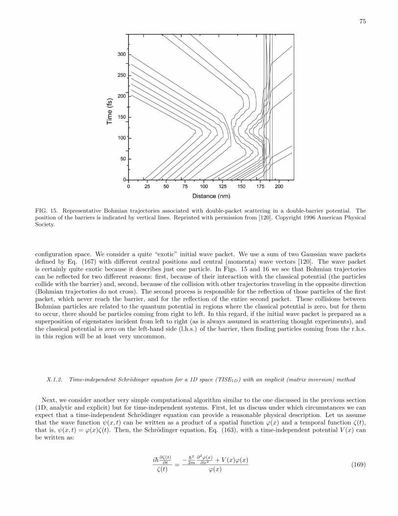
75

FIG. 15. Representative Bohmian trajectories associated with double-packet scattering in a double-barrier potential. Theposition of the barriers is indicated by vertical lines. Reprinted with permission from [120]. Copyright 1996 American PhysicalSociety.

configuration space. We consider a quite “exotic” initial wave packet. We use a sum of two Gaussian wave packetsdefined by Eq. (167) with different central positions and central (momenta) wave vectors [120]. The wave packetis certainly quite exotic because it describes just one particle. In Figs. 15 and 16 we see that Bohmian trajectoriescan be reflected for two different reasons: first, because of their interaction with the classical potential (the particlescollide with the barrier) and, second, because of the collision with other trajectories traveling in the opposite direction(Bohmian trajectories do not cross). The second process is responsible for the reflection of those particles of the firstpacket, which never reach the barrier, and for the reflection of the entire second packet. These collisions betweenBohmian particles are related to the quantum potential in regions where the classical potential is zero, but for themto occur, there should be particles coming from right to left. In this regard, if the initial wave packet is prepared as asuperposition of eigenstates incident from left to right (as is always assumed in scattering thought experiments), andthe classical potential is zero on the left-hand side (l.h.s.) of the barrier, then finding particles coming from the r.h.s.in this region will be at least very uncommon.

X.1.2. Time-independent Schrodinger equation for a 1D space (TISE1D) with an implicit (matrix inversion) method

Next, we consider another very simple computational algorithm similar to the one discussed in the previous section(1D, analytic and explicit) but for time-independent systems. First, let us discuss under which circumstances we canexpect that a time-independent Schrodinger equation can provide a reasonable physical description. Let us assumethat the wave function ψ(x, t) can be written as a product of a spatial function ϕ(x) and a temporal function ζ(t),that is, ψ(x, t) = ϕ(x)ζ(t). Then, the Schrodinger equation, Eq. (163), with a time-independent potential V (x) canbe written as:

ih∂ζ(t)∂t

ζ(t)=− h2

2m∂2ϕ(x)∂x2 + V (x)ϕ(x)

ϕ(x)(169)

76

0 50 100 150 200

t=300 fs

t=200 fs

t=120 fs

t=60 fs

t=20 fs

Pres

ence

pro

babi

lity

(a.u

.)

Distance (nm)

FIG. 16. Picture motion of the same double-packet wave function considered in Fig. 15, calculated by numerical integrationof the time-dependent Schrodinger equation. Five representative “snapshots” obtained at different times are shown with thevertical scale arbitrarily changed in each case for clarity. Although the norm of the wave function is always unity, it does notseem so because of the changes in the scale. The marks are visual aids that indicate the position of some related Bohmiantrajectories shown in Fig. 15. The double-barrier position is indicated by the vertical dashed lines, and the arrows indicate thesense of motion of the two packets. Reprinted with permission from [120]. Copyright 1996 American Physical Society.

Since the l.h.s. of Eq. (169) only depends on t and the r.h.s. of Eq. (169) only depends on x, both sides are equal toa constant that we refer as E. Therefore, we obtain two separate equations:

ih∂ζ(t)

∂t= Eζ(t) (170)

− h2

2m

∂2ϕ(x)

∂x2+ V (x)ϕ(x) = Eϕ(x) (171)

The first of these equations has a trivial analytical solution ζ(t) = eiEth . However, the time-independent Schrodinger

equation needs a numerical method to be solved for arbitrary shapes of the potential V (x).

The second-order derivative can be approximated as:

∂2ϕ (x)

∂x2

∣∣∣∣x=xk

≈ ϕ(xk+1)− 2ϕ(xk) + ϕ(xk−1)

∆x2 (172)

Then, Eq. (171) can be written in a matrix representation as:

(− h2

2m∇2 + (V (xk)− E) I

)~ϕ = 0 (173)

where ~ϕ = (ϕ(x2), . . . , ϕ(xN−1))T is a N − 2 vector, I is the (N − 2) × (N − 2) identity matrix and ∇2 is the

77

(N − 2)× (N − 2) matrix constructed from Eq. (172) as:

∇2 =1

∆x2

−2 1 0 0. . .

1 −2 1 0. . .

. . .. . .

. . .. . .

. . .

. . . 0 1 −2 1

. . . 0 0 1 −2

(174)

The solution of ~ϕ can be found by inverting the matrix equation, Eq. (173). The (nonzero) solution of Eq. (173)requires that the determinant of the matrix be equal to zero. The determinant requirement is called the characteristicequation (less often, the secular equation). In our case, the determinant can only be zero for some particular valuesof the energy E (i.e., quantized energies). Thus, this algorithm finds the eigenvalues E and eigenvectors ~ϕ, typical ofa boundary value problem.44

In the previous vector definition, ~ϕ, only N − 2 unknowns are considered. We have assumed that ϕ(x1) = 0 andϕ(xN ) = 0. This implies that ~ϕ is a real vector. Then, if we select an eigenstate, we realize that the current densityis zero, J(x, t) = 0, because ϕ(xk) = ϕ(xk)∗. All Bohmian velocities are zero, ∂S/∂x = 0, meaning that Bohmiantrajectories do not “move.” This result is obviously consistent with the fact that the amplitude R(x, t) of the globalwave function ψ(x, t) = ϕ(x)e−iEt/h is time independent. One is tempted to affirm that there is no kinetic energyfor these Bohmian trajectories. However, as we see in Eq. (136), the evaluation of the mean value of the kineticenergy takes into account not only the Bohmian velocity but also the quantum potential. We can explain this point,differently, from the quantum Hamilton–Jacobi equation, Eq. (39). In our particular time-independent case, we havean energy conservation law:

V (x)− h2

2m

∂2R(x)/∂x2

R(x)= E

where we have used ∂S/∂t = −E in Eq. (39). Then, we can obtain the following (time-independent Schrodinger-like)equation for the real wave function R(x):

− h2

2m

∂2R(x)

∂x2+ V (x)R(x) = E R(x) (175)

Comparing this expression with the previous Eq. (171), we realize that in this particular problem (for which allBohmian trajectories have zero velocity), the quantum potential takes the role of a “kinetic” energy.

X.1.3. Time-independent Schrodinger equation for a 1D space (TISE1D) with an explicit method

We can also look for a very simple explicit algorithm to find the solution ~ϕ of the time-independent Schrodingerequation. Equation (171) is a homogeneous second-order differential equation that can be written as:

d2

dx2ϕ(x) = f(x)ψ(x) (176)

where f(x) is the constant of proportionality between the solution and the second derivative at each point:

f(x) =2m

h2 (V (x)− E) (177)

From the Taylor expansion for ϕ(xk+1) around xk, we get:

ϕ(xk+1) =ϕ(xk) + ∆xdϕ(x)

dx

∣∣∣∣x=xk

+∆x2

2!

d2ϕ(x)

dx2

∣∣∣∣x=xk

+∆x3

3!

d3ϕ(x)

dx3

∣∣∣∣x=xk

+∆x4

4!

d4ϕ(x)

dx4

∣∣∣∣x=xk

+∆x5

5!

d5ϕ(x)

dx5

∣∣∣∣x=xk

+O(h6) (178)

44 The practical implementation of this algorithm can be done, for example, quite easily with the software MATLAB. The instruction[V,D] = eig(A) produces matrices of eigenvalues (D) and eigenvectors (V) of matrix A, so that A ∗ V = V ∗D. Equation (173) canbe rewritten as A ∗ V = V ∗D.

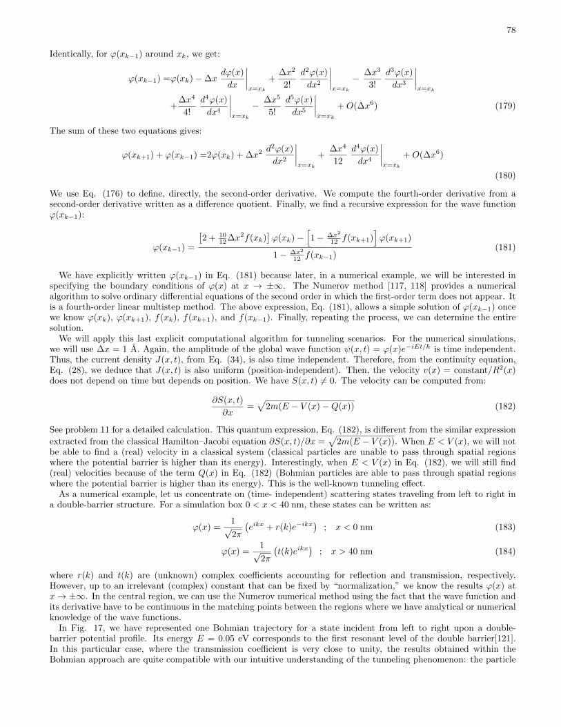
78

Identically, for ϕ(xk−1) around xk, we get:

ϕ(xk−1) =ϕ(xk)−∆xdϕ(x)

dx

∣∣∣∣x=xk

+∆x2

2!

d2ϕ(x)

dx2

∣∣∣∣x=xk

− ∆x3

3!

d3ϕ(x)

dx3

∣∣∣∣x=xk

+∆x4

4!

d4ϕ(x)

dx4

∣∣∣∣x=xk

− ∆x5

5!

d5ϕ(x)

dx5

∣∣∣∣x=xk

+O(∆x6) (179)

The sum of these two equations gives:

ϕ(xk+1) + ϕ(xk−1) =2ϕ(xk) + ∆x2 d2ϕ(x)

dx2

∣∣∣∣x=xk

+∆x4

12

d4ϕ(x)

dx4

∣∣∣∣x=xk

+O(∆x6)

(180)

We use Eq. (176) to define, directly, the second-order derivative. We compute the fourth-order derivative from asecond-order derivative written as a difference quotient. Finally, we find a recursive expression for the wave functionϕ(xk−1):

ϕ(xk−1) =

[2 + 10

12∆x2f(xk)]ϕ(xk)−

[1− ∆x2

12 f(xk+1)]ϕ(xk+1)

1− ∆x2

12 f(xk−1)(181)

We have explicitly written ϕ(xk−1) in Eq. (181) because later, in a numerical example, we will be interested inspecifying the boundary conditions of ϕ(x) at x → ±∞. The Numerov method [117, 118] provides a numericalalgorithm to solve ordinary differential equations of the second order in which the first-order term does not appear. Itis a fourth-order linear multistep method. The above expression, Eq. (181), allows a simple solution of ϕ(xk−1) oncewe know ϕ(xk), ϕ(xk+1), f(xk), f(xk+1), and f(xk−1). Finally, repeating the process, we can determine the entiresolution.

We will apply this last explicit computational algorithm for tunneling scenarios. For the numerical simulations,we will use ∆x = 1 A. Again, the amplitude of the global wave function ψ(x, t) = ϕ(x)e−iEt/h is time independent.Thus, the current density J(x, t), from Eq. (34), is also time independent. Therefore, from the continuity equation,Eq. (28), we deduce that J(x, t) is also uniform (position-independent). Then, the velocity v(x) = constant/R2(x)does not depend on time but depends on position. We have S(x, t) 6= 0. The velocity can be computed from:

∂S(x, t)

∂x=√

2m(E − V (x)−Q(x)) (182)

See problem 11 for a detailed calculation. This quantum expression, Eq. (182), is different from the similar expression

extracted from the classical Hamilton–Jacobi equation ∂S(x, t)/∂x =√

2m(E − V (x)). When E < V (x), we will notbe able to find a (real) velocity in a classical system (classical particles are unable to pass through spatial regionswhere the potential barrier is higher than its energy). Interestingly, when E < V (x) in Eq. (182), we will still find(real) velocities because of the term Q(x) in Eq. (182) (Bohmian particles are able to pass through spatial regionswhere the potential barrier is higher than its energy). This is the well-known tunneling effect.

As a numerical example, let us concentrate on (time- independent) scattering states traveling from left to right ina double-barrier structure. For a simulation box 0 < x < 40 nm, these states can be written as:

ϕ(x) =1√2π

(eikx + r(k)e−ikx

); x < 0 nm (183)

ϕ(x) =1√2π

(t(k)eikx

); x > 40 nm (184)

where r(k) and t(k) are (unknown) complex coefficients accounting for reflection and transmission, respectively.However, up to an irrelevant (complex) constant that can be fixed by “normalization,” we know the results ϕ(x) atx→ ±∞. In the central region, we can use the Numerov numerical method using the fact that the wave function andits derivative have to be continuous in the matching points between the regions where we have analytical or numericalknowledge of the wave functions.

In Fig. 17, we have represented one Bohmian trajectory for a state incident from left to right upon a double-barrier potential profile. Its energy E = 0.05 eV corresponds to the first resonant level of the double barrier[121].In this particular case, where the transmission coefficient is very close to unity, the results obtained within theBohmian approach are quite compatible with our intuitive understanding of the tunneling phenomenon: the particle

79

0,0

0,2

0,4(a)

Pot

entia

l Ene

rgy

(eV

)

Trajectory

0 10 20 30 40

0,0

0,2

(b)

Distance (nm)

Trajectory

0

1000

2000

3000

Total potential

Classicalpotential

Tim

e (fs

)

0

2000

4000

Total potential

Classicalpotential

FIG. 17. Bohmian trajectories associated with stationary scattering states impinging on a typical GaAs/AlGaAs RTD with2 nm barriers of 0.3 eV separated by a 7 nm well. The classical potential and the total potential (the sum of classicaland quantum terms) are also depicted in dashed and solid lines, respectively. (a) Resonant eigenstate, Ek = 0.05 eV; (b)nonresonant eigenstate, Ek = 0.06 eV. Reprinted with permission from [121]. Copyright 1996 Elsevier. Abbreviation: RTD,resonant tunneling diode.

is transmitted, and its velocity decreases in the well. We do also plot the total potential-that is, the sum V (x)+Q(x)-which is lower than the electron energy E = 0.05 eV.

However, the situation is far from intuitive for nonresonant states. In Fig. 17b, we have represented one of thesenonresonant trajectories for the same potential profile. Now, although the transmission coefficient is much smallerthan unity for the nonresonant states, they present the same features as the resonant ones: all Bohmian trajectoriesare transmitted through the barrier. This fact can be easily understood from a mathematical point of view. As wementioned, the current and particle densities are time independent and positive everywhere. So, the Bohmian velocityis always positive. In this regard, although Bohmian trajectories associated with scattering states perfectly reproducethe presence probability and the current density, they do not reproduce our particle-intuitive understanding of thetunneling phenomenon, since in principle, we would expect reflected as well as transmitted trajectories. The originof this lack of intuitive behavior of Bohmian trajectories is only due to the initial wave function that we select. Thevelocity of Bohmian particles is neither related to the incident electron nor related to the reflected one but to theaverage of both because the wave function itself is defined as a weighted sum of waves with positive and negativemomentum. In particular, if the barrier is infinitely high, then the reflection coefficient is equal to one and Bohmian’svelocity is zero (one would expect positive and negative electron velocities). Transport is better formulated as atime-dependent process. A time dependent picture of transport involves a wave packet with a well defined initialvelocity and, after the interaction, a well-defined reflected (or transmitted) velocity, but not a unique velocity withan average of incident and reflected velocities.

All the 1D numerical algorithms previously discussed can be easily generalized to 2D and 3D systems (see, forexample, the solution of the Schrodinger equation for computing Bohmian trajectories in atomic scenarios in Refs.[122, 123]). However, the computational burden of such techniques with finite-difference meshes is enormous, and thesolution using adaptative meshes seems interesting. For example, the triangular mesh generated using an algorithminspired by Ref. [124], with Delaunay refinement algorithms, yields a final mesh that is surprisingly well shaped,resulting in an excellent support to solve partial differential equations, as it was remarked in Ref. [125].

X.2. Synthetic computation of Bohmian trajectories

Up to here, we have only discussed analytical algorithms to find Bohmian trajectories. However, it is possi-ble to compute Bohmian trajectories without knowing the wave function. The key point is using the polar formψ(~r, t) = R(~r, t) exp(iS(~r, t)/h) to obtain the quantum Hamilton–Jacobi equations. As we anticipated, these newequations are nonlinear in R(~r, t) and S(~r, t). We will now discuss the advantages and disadvantages of numerically

80

solving the quantum Hamilton–Jacobi equation, Eq. (39). Hereafter, we will analyze two different algorithms to solvenumerically Eq. (39). First, directly solving these equations (the Eulerian formalism) or some equivalent variablechange . Second rewriting the Hamilton–Jacobi equations within the Langrangian formalism and solving them.

The first point that we want to clarify is that, although the function S(~r, t) is in principle multivalued, the numericalsolution of S(~r, t) has a unique value at each point ~r and t. The reason is because of an important theorem on theexistence and uniqueness of solutions to first-order equations with given initial-value problems. See page 70 in [126].

X.2.1. Time-dependent quantum Hamilton–Jacobi equations (TDQHJE1D) with an implicit (Newton-like fixed Eulerianmesh) method

In the Eulerian formalism, we use a fixed grid. We are interested in providing a discussion valid for 1D, 2D, and3D spatial scenarios. Therefore, we define a grid in real space through a set of discrete vectors ~pi for i = 1, . . . , N -inparticular, ~pi = (xi, yi, zi) for a 3D space, ~pi = (xi, yi) for a 2D space, and ~pi = (xi) for 1D. In order to provide acompact notation, we define:

~Rj = (Rj(~p1), . . . , Rj(~pN ))T

(185)

~Sj = (Sj(~p1), . . . , Sj(~pN ))T

(186)

~Vj = (Vj(~p1), . . . , Vj(~pN ))T

(187)

where Rj(~pi) = R(~r, t) at t = tj and ~r = ~pi (identically for Sj(~pi) = S(~r, t) and Vj(~pi) = V (~r, t)). We have also useda mesh in time tj = j∆t for j = 1, . . . ,M

In the definition of the temporal derivatives of the quantum Hamilton–Jacobi, we can use an implicit expression,Eq. (162), or an explicit one, Eq. (160). The explicit expression will lead to an algorithm similar to the one describedin Sec. X.1.1 with the same advantages (simplicity) and disadvantages (i.e., conditional stable). In this section, wewill explore the implicit route. Then, the discrete version of the quantum Hamilton–Jacobi equations, Eq. (39), reads:

~R2j − ~R2

j−1

∆t+ ∇

(~R2j ∇~Sjm

)= 0

(188)

~Sj − ~Sj−1

∆t+

(∇~Sj)2

2m− h2

2m

∇2 ~Rj~Rj

+ ~Vj = 0

The operations such as power, multiplication, and division between the vectors ~Xj and ~Yj are understood over eachpoint in the spatial mesh, that is:

~Xj~Yj = [Xj(~p1)Yj(~p1), . . . , Xj(~pN )Yj(~pN )]T (189)

Here the symbol ∇ is the matrix representation of the differential operator ~∇ in the 1D, 2D, or 3D spatial mesh.The representation of ∇ depends in general on the choice of the spatial mesh and on how the spatial derivatives areapproximated. For example, in a 1D system with a uniform mesh step size ∆x, the discrete version of the spatialderivative in one dimension is:

∂R(x, t)

∂x=Rj(~pi+1)−Rj(~pi−1)

2∆x, (190)

with ~pi = x0 + i∆x. Then, the nabla operator in one dimension ∇1D is represented by the following matrix:

∇1D =1

2∆x

2 −2 0 0. . .

1 0 −1 0. . .

. . .. . .

. . .. . .

. . .

. . . 0 1 0 −1

. . . 0 0 −2 2

(191)

Notice that we have changed the definition of the spatial derivative from Eq. (190) in x1 and xN . In two or threedimensions the matrices still have many zeros with the entries 1 and −1 properly located.

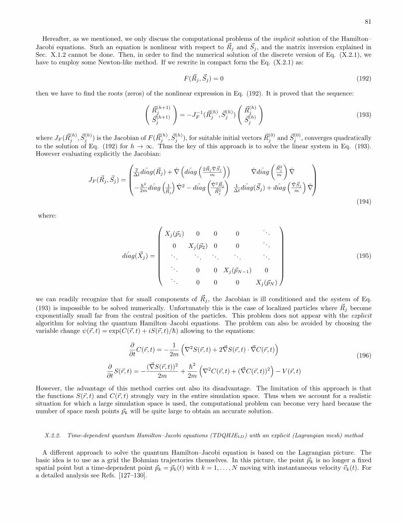
81

Hereafter, as we mentioned, we only discuss the computational problems of the implicit solution of the Hamilton–

Jacobi equations. Such an equation is nonlinear with respect to ~Rj and ~Sj , and the matrix inversion explained inSec. X.1.2 cannot be done. Then, in order to find the numerical solution of the discrete version of Eq. (X.2.1), wehave to employ some Newton-like method. If we rewrite in compact form the Eq. (X.2.1) as:

F (~Rj , ~Sj) = 0 (192)

then we have to find the roots (zeros) of the nonlinear expression in Eq. (192). It is proved that the sequence:(~R

(h+1)j

~S(h+1)j

)= −J−1

F (~R(h)j , ~S

(h)j )

(~R

(h)j

~S(h)j

)(193)

where JF (~R(h)j , ~S

(h)j ) is the Jacobian of F (~R

(h)j , ~S

(h)j ), for suitable initial vectors ~R

(0)j and ~S

(0)j , converges quadratically

to the solution of Eq. (192) for h → ∞. Thus the key of this approach is to solve the linear system in Eq. (193).However evaluating explicitly the Jacobian:

JF (~Rj , ~Sj) =

2

∆tˆdiag(~Rj) + ∇

(ˆdiag(

2~Rj∇~Sjm

))∇ ˆdiag

(~R2j

m

)∇

− h2

2mˆdiag(

1~Rj

)∇2 − ˆdiag

(∇2 ~Rj~R2j

)1

∆tˆdiag(~Sj) + ˆdiag

(∇~Sjm

)∇

(194)

where:

ˆdiag( ~Xj) =

Xj(~p1) 0 0 0. . .

0 Xj(~p2) 0 0. . .

. . .. . .

. . .. . .

. . .

. . . 0 0 Xj(~pN−1) 0

. . . 0 0 0 Xj(~pN )

(195)

we can readily recognize that for small components of ~Rj , the Jacobian is ill conditioned and the system of Eq.

(193) is impossible to be solved numerically. Unfortunately this is the case of localized particles where ~Rj becomeexponentially small far from the central position of the particles. This problem does not appear with the explicitalgorithm for solving the quantum Hamilton–Jacobi equations. The problem can also be avoided by choosing thevariable change ψ(~r, t) = exp(C(~r, t) + iS(~r, t)/h) allowing to the equations:

∂

∂tC(~r, t) = − 1

2m

(∇2S(~r, t) + 2~∇S(~r, t) · ~∇C(~r, t)

)(196)

∂

∂tS(~r, t) = − (~∇S(~r, t))2

2m+h2

2m

(∇2C(~r, t) + (~∇C(~r, t))2

)− V (~r, t)

However, the advantage of this method carries out also its disadvantage. The limitation of this approach is thatthe functions S(~r, t) and C(~r, t) strongly vary in the entire simulation space. Thus when we account for a realisticsituation for which a large simulation space is used, the computational problem can become very hard because thenumber of space mesh points ~pk will be quite large to obtain an accurate solution.

X.2.2. Time-dependent quantum Hamilton–Jacobi equations (TDQHJE1D) with an explicit (Lagrangian mesh) method

A different approach to solve the quantum Hamilton–Jacobi equation is based on the Lagrangian picture. Thebasic idea is to use as a grid the Bohmian trajectories themselves. In this picture, the point ~pk is no longer a fixedspatial point but a time-dependent point ~pk = ~pk(t) with k = 1, . . . , N moving with instantaneous velocity ~vk(t). Fora detailed analysis see Refs. [127–130].

82

To pass from the Eulerian to the Lagrangian hydrodynamic picture, we must be careful with the time derivative ofthe functions R(~pk(t), t), S(~pk(t), t) and V (~pk(t), t). We have to use the chain rule:

d

dt=

∂

∂t+ ~v(~r, t) · ~∇ (197)

which includes the convective term ~v(~r, t) · ~∇ with the velocity defined:

~v(~r, t) =1

m~∇S(~r, t) (198)

The new equations derived from the quantum Hamilton–Jacobi equations (or equivalently from Eq. (X.2.1)) can bewritten as:

d

dt~pk(t) = ~v(~pk(t), t) (199)

d

dtS(~pk(t), t) =

(~∇S(~pk(t), t))2

2m+h2

2m

∇2R(~pk(t), t)

R(~pk(t), t)− V (~pk(t), t) (200)

~v(~pk(t), t) =1

m~∇S(~pk(t), t) (201)

d

dtR(~pk(t), t) = −1

2R(~pk(t), t)~∇ · ~v(~pk(t)) (202)

The differential system in Eqs. (199–202) is written for the trajectory ~pk(t) with a particular initial position ~pk(0).However to (numerically) reproduce the wave function ψ(~r, t) = R(~r, t) exp(iS(~r, t)/h) defined in the entire space, wehave to deal with k = 1, . . . , N trajectories with N → ∞. The distribution of their initial positions ~pk(0) has to beobtained according to the squared modulus of the initial wave function |ψ(~pk(0), 0)|2, that is, the quantum equilibriumhypothesis described in Sec. V.6. See also Ref. [24]. Thus, by construction we are using a mesh that is continuouslyadapting to the wave function time evolution because the Bohmian trajectories themselves follow the wave function.

In this picture the strategy to solve Eqs. (199–202) can be very complicated [127–130]. However, some simpleconsideration can be done in order to understand the limits of this approach. The method widely used [127–130] tointegrate Eqs. (199–202) is to solve them in cascade with the following approximations: at time tj the new trajectoriespositions are computed through:

~pj,k = ~pj−1,k + ∆t~vj−1,k (203)

with ~pj,k = ~pk(tj). In the updated grid defined by ~pj,k, the variables Sj(~pj,k), ~vj(~pj,k), and ~Rj(~pj,k) are evaluated by:

Sj(~pj,k) = Sj−1(~pj,k) + ∆t

[(∇j−1Sj−1(~pj,k))2

2m+

h2

2m

∇2j−1Rj−1(~pj,k)

Rj−1(~pj,k)− ~Vj−1(~pj,k)

]

Rj(~pj,k) = Rj−1(~pj,k)−∆t

[1

2mRj−1(~pj,k)∇2

j−1~Sj−1(~pj,k)

]vj(~pj,k) =

1

m∇j ~Sj(~pj,k)

where ∇j is the gradient operator evaluated in ~pj,k through efficient interpolation methods [127–130]. It can be realizedthat we have used an (unstable) explicit (forward Euler) time integration method [131] to avoid the computationalburden associated with implicit methods with nonlinear equations discussed before. This limitation (small temporalstep to ensure stable solutions) is made worse since the time step must be further reduced when some trajectoryapproaches points for which the potential V and/or the quantum potential Q strongly varies provoking large variationsof some ~vj .

The variables S and ~v vary in the entire simulation space; thus when we account for a realistic situation such thata large simulation space is used, the computational problem can become very hard due to the fact that the number ofspace mesh points ~pk can diverge to obtain an accurate solution. On the contrary, this method has some fundamentaladvantage over methods using fix grid points. In the latter, the extension of 1D algorithms to 2D and 3D algorithmsmeans increasing exponentially the number of grip points. However, in the former methods (i.e., when the grid pointsare Bohmian trajectories), the number of points can be chosen by the user. Thus, for exemple, one can simulate a 1Dsystem with 1,000 Bohmian trajectories (grid points) and a 2D system with 3,000 Bohmian trajectories (grid points).

83

X.3. More elaborated algorithms

We have presented very simple and easily implementable codes for computing Bohmian trajectories in simplescenarios. These algorithms can be used for newcomers to be introduced to the computation of quantum dynamicswith Bohmian mechanics. Certainly, there are many more elaborated and “professional” computational algorithmsin the literature. An excellent source of information on this issue can be found in the book written by R. E. Wyattentitled Quantum Dynamics with Trajectories: Introduction to Quantum Hydrodynamics [20].

To end this section, we want to briefly mention some original and powerful techniques, inspired by Bohmianmechanics, available in the literature, whose explicit description is far from the scope of this introductory appendix.Recently, B. Poirier showed how Bohmian trajectories can be computed for 1D eigenstates without the wave function[133]. The work of N. Makri shows the possibility of using imaginary time algorithms to estimate eigenstates andeigenvalues [135]. With a similar goal, I. P. Christov uses quantum trajectories to develop time-dependent quantumMonte Carlo algorithms [136, 137]. We also mention the work of E. L. Bittner [138] developed in chapter 5 in this book.The work presented in Sec. VI.6 can also be interpreted as an approximating technique for computing many-particlesystems [94]. This last work has been used by the group of Oriols to develop a powerful quantum electron transportsimulator. ( http://europe.uab.es/bitlles). See Refs. [140, 141] or chapter 6 for practical results on electron correlationin nanoelectronics. Another line of work is also devoted to the approximation of the quantum potential. See, forexample, the work of S. Garashchuk and V. A. Rassolov [139]. The correlation between classical and quantum systemshas also been studied extensively. See, for example, Ref. [142–144]. We do also highlight the work by D. J. Tannorand coworkers on the use of imaginary quantum trajectories (complex action) for quantum dynamics [132, 134]. Wealso want to notice the important amount of work done by many people in the field of ab-initio molecular dynamics,specially for tackling the coupled electron-nuclear motion in nonadiabatic electronic transitions [145–151]. Finally, wemention the more recent work by L. B. Madsen and co-workers in the field of bosonic systems [152].

All the works mentioned have been elaborated during the past 18 years after the pioneering work of Wyatt [127,153]. Much work is still needed to evaluate the real capability of synthetic applications of Bohmian mechanics as acomputational tool.

[1] M. Planck, On the Law of Distribution of Energy in the Normal Spectrum, Annalen der Physik 4, 553 (1901).[2] A. Einstein, ber einen die Erzeugung und Verwandlung des Lichtes betreffenden heuristischen Gesichtspunkt, Annalen der

Physik 17, 132 (1905).[3] N. Bohr, On the Constitution of Atoms and Molecules, Part I, Philosophical Magazine 26, 1 (1913).[4] N. Bohr, On the Constitution of Atoms and Molecules, Part II Systems Containing Only a Single Nucleus, Philosophical

Magazine 26, 476 (1913).[5] N. Bohr, On the Constitution of Atoms and Molecules, Part III Systems Containing Several Nuclei, Philosophical Magazine

26, 857 (1913).[6] L. de Broglie, Recherches sur la theorie des quantas, Ann. de Physique 3, 22 (1925).[7] L. de Broglie La mecanique ondulatorie et la structure atomique de la matiere et du rayonnement, Journal de Physique

et du Radium 8, 225 (1927).[8] D. Bohm, A suggested interpretation of the quantum theory in terms of “hidden” variables I, Phys. Rev. 85, 166 (1952).[9] D. Bohm, A suggested interpretation of the quantum theory in terms of “hidden” variables II, Phys. Rev. 85, 180, (1952).

[10] M. Born, Zur Quantenmechanik der Stovorgange, Zeitschrift fur Physik 37, 863 (1926).

[11] W. Heisenberg, Uber quantentheoretishe Umdeutung kinematisher und mechanischer Beziehungen, Zeitschrift fur Physik33, 879 (1925); English translation in Ref. [33].

[12] J. von Neumann, Mathematische Grundlagen der Quantenmechanik (Springer Verlag, Berlin 1932); English translationby: R. T. Beyer, Mathematical Foundations of Quantum Mechanics (Princeton University Press, Princeton 1955).

[13] J. S. Bell, 1987, Speakable and Unspeakable in Quantum Mechanics (Cambridge University Press, Cambridge 1987).[14] A. Einstein, Physics and reality Journal of the Franklin Institute 221(3), 349 (1936).[15] E. Wigner, The Unreasonable Effectiveness of Mathematics in the Natural Sciences, Communications on Pure and Applied

Mathematics 13, 1 (1960).[16] N. Herbert, Quantum reality (Anchor Books, New York 1984).[17] “If, in some cataclysm, all of scientific knowledge were to be destroyed, and only one sentence passed on to the next

generations of creatures, what statement would contain the most information in the fewest words? I believe it is theatomic hypothesis (or the atomic fact, or whatever you wish to call it) that all things are made of atoms—little particlesthat move around in perpetual motion, attracting each other when they are a little distance apart, but repelling uponbeing squeezed into one another. In that one sentence, you will see, there is an enormous amount of information aboutthe world, if just a little imagination and thinking are applied.” R. P. Feynman, R. B. Leighton and M. Sands, FeynmanLectures on Physics (Addison-Wesley, Caltech USA 1965).

References 84

[18] G. Binnig, H. Rohrer, C. Gerber, and E.Weibel, Surface Studies by Scanning Tunneling Microscopy, Physical ReviewLetters 49, 57 (1982).

[19] Private exchange of letters between S. Goldstein and S. Weinberg; http://www.mathematik.uni-muenchen.de/

~bohmmech/BohmHome/weingold.htm

[20] R. E. Wyatt Quantum Dynamics with Trajectories: Introduction to Quantum Hydrodynamics (Springer, 2005).[21] A. Valentini, Pilot-Wave Theory: An Alternative Approach to Modern Physics (Cambridge University Press, Cambridge

2006).[22] G. Bacciagaluppi and A. Valentini, Quantum Theory at the Cross-roads: Reconsidering the 1927 Solvay Conference

(Cambridge University Press, Cambridge 2009).[23] D. Peat Infinite Potential: the life and times of David Bohm (Helix Books, Addison-Wesley Publishing Company, Inc.

1997)[24] P. R. Holland, The Quantum Theory of Motion: An account of the de Broglie-Bohm Causal Interpretation of Quantum

mechanics (Cambridge University Press, Cambridge 1993).[25] S. W. Saunders et al. Everett and his Critics (Oxford University Press, 2009) and arXiv: quant-ph/0811081.[26] J. T. Cushing, A. Fine and S. Goldstein, Bohmian Mechanics and Quantum Theory: An Appraisal (Kluwer Academic

Publishers, 1996)[27] Private communication with Basile Hiley and David Peat[28] D. Bohm and B. J. Hiley. The Uundivided Universe: An Ontological Intepretation of Quantum Theory (Routledge &

Kegan Paul, London, 1993).[29] E. Madelung, Quantentheorie in hydrodynamischer Form, Z. Phys. 40, 322 (1926).[30] http://www.isiknowledge.com/

[31] L. de Broglie, Recherches sur la theorie des quantas, PhD thesis, University of Paris (1924); see also [6].[32] G. N. Lewis, The Conservation of Photons, Nature 118(2), 874 (1926); See also http://www.nobeliefs.com/photon.htm[33] B. L. van der Waerden, Sources of Quantum Mechanics (Dover Publications, 1968).

[34] W. Heisenberg, Uber den anschaulichen Inhalt der quantentheoretischen Kinematik und Mechanik, Zeitschrift fur Physik43(3–4), 172 (1927).

[35] M. Born and P. Jordan, Zur Quantenmechanik, Zeitschrift fur Physik 34, 858 (1925); English translation in Ref. [33].[36] M. Born, W. Heisenberg, and P. Jordan, Zur Quantenmechanik II, Zeitschrift fur Physik 35, 557 (1925); English trans-

lation in Ref. [33].[37] E. Schrodinger, An Undulatory Theory of the Mechanics of Atoms and Molecules, Physical Review 28, 1049 (1926).[38] B. L. van der Waerden, From Matrix Mechanics and Wave Mechanics to Unified Quantum Mechanics, Notices of the

AMS 44, 323 (1997).[39] D. Bohm, Quantum Theory (Dover Publications, New York, 1951).[40] N. D. Mermin, What’s Wrong with This Pillow?, Physics Today 42(4), 9 (1989).[41] N. D. Mermin, Could Feynman Have Said This?, Physics Today 57(5), 10 (2004).[42] L. de Broglie, Tentative d’interpretation causale et non-lineairie de la mecanique ondulatorie (Gauthier-Villars, Paris,

1956).[43] http://www.alberteinstein.info/db/ViewDetails.do?DocumentID = 34338; explained also in [44].[44] P. R, Holland, What’s Wrong with Einstein’s 1927 Hidden-Variable Interpretation of Quantum Mechanics?, Foundations

of Physics, 35(2) 177 (2005).[45] D. Bohm, on an interview in 1987; see http://www.fdavidpeat.com/interviews/bohm.htm[46] A. Einstein, B. Podolsky, and N. Rosen, Can Quantum Mechanical Description of the Physical Reality Be Considered

Complete? Physics Review 47, 777 (1935).[47] C. Cohen-Tanoudji, B. Diu, and F. Laloe, Quantum Mechanics (Wiley, New York, 1977).[48] H. Nikolic, Would Bohr Be Born if Bohm Were Born before Born?, Am. J. Phys. 76, 143 (2008).[49] M. Gell-Mann, The Nature of the Physical Universe: The 1976 Nobel Conference (Wiley, New York, 1979); M. Gell-Mann

presented his Nobel lecture but did not submit the manuscript for inclusion in the official volume. He explains: I did havea written version of the lecture that I gave in Sweden, but I was not satisfied with it and did not submit it . . . I tried towrite a better one, including an adequate discussion of quarks, and agonized over it for months, but in the end, I did notfinish it in time for it to be included in the volume..

[50] J. S. Bell, On the Einstein Podolsky Rosen Paradox Physics 1, 195 (1964).[51] J. S. Bell, On the Impossible Pilot Wave, Foundations of Physics 12, 989 (1982). Reprinted in [13].[52] J. S. Bell, Against Measurement, Physics World 3, 33 (1990).[53] H. P. Stapp, Are Superluminal Connections Necessary?, Il Nuovo Cimento 40B, 191 (1977).[54] A. Aspect, P. Grangier, and G. Roger, Experimental Realization of Einstein-Podolsky-Rosen-Bohm Gedankenexperiment:

A New Violation of Bell’s Inequalities, Physical Review Letters 49(2), 91 (1982).[55] D. Kleppner and R. Jackiw, One Hundred Years of Quantum Physics, Science 289(5481), 893 (2000).[56] T. Takabayasi, On the Formulation of Quantum Mechanics Associated with Classical Pictures, Progress of Theoretical

Physics 8, 143 (1952).[57] It is written in Ref. [26] by Professor J. T. Cushing, himself, that he submitted a research proposal to the US National

Science Foundation for theoretical work to be done, within the framework of Bohm’s version of quantum theory, on somefoundational questions in quantum mechamics and received the following evaluation The subject under consideration, therival Copenhagen and causal (Bohm) interpretations of the quantum theory, has been discussed for many years and in the

References 85

opinion of several members of the Physics Division of the NSF, the situation has been settled. The causal interpretationis inconsistent with experiments which test Bell’s inequalities. Consequently . . . funding . . . a research program in this areawould be unwise.

[58] G. Brida, E. Cagliero, G. Falzetta, M. Genovese, M. Gramegna, and E. Predazzi, Biphoton Double-Slit Experiment,Physical Review A 68, 033803 (2003).

[59] X. Oriols, Comment on “Biphoton Double-Slit Experiment”, Physical Review A 71, 017801 (2005).[60] P. A. Schilpp, Discussion with Einstein on epistemological problems in atomic physics in The Library of Living Philoso-

phers, Volume 7. Albert Einstein: Philosopher-Scientist, pp. 199–241 (Open Court, La Salle-Illinois).[61] D. Bohm, Proof that Probability Density Approaches |ψ|2 in Causal Interpretation of Quantum Theory, Physical Review

89, 458 (1953).[62] W. Struyve, The de Broglie–Bohm Pilot-Wave Interpretation of Quantum Theory PhD thesis, Universiteit Gent (2004)

and also in arXiv:quant-ph/0506243.7[63] D. Durr, S. Goldstein, R. Tumulka, and N. Zanghı, Bohmian Mechanics and Quantum Field Theory, Physical Review

Letters 93(9), 090402 (2004).[64] D. Durr, S. Goldstein, R. Tumulka, and N. Zanghı, Trajectories and Particle Creation and Annihilation in Quantum Field

Theory, Journal of Physics A - Matemathical and General 36(14), 4143 (2003).[65] R. P. Feynman, R. B. Leighton, and M. Sands, The Feynman Lectures on Physics, I, II and III (Addison-Wesley, New

York, 1963).[66] H. M. Wiseman, Grounding Bohmian mechanics in weak values and bayesianism New Journal of Physics 9, 165 (2007).[67] D. Marian, N. Zanghı, X. Oriols, Weak Values from Displacement Currents in Multiterminal Electron Devices, Phys. Rev.

Lett. 116, 110404 (2016) and also in arXiv:1508.00248.[68] E. Colomes, Z.Zhan, X. Oriols Comparing Wigner, Husimi and Bohmian distributions: Which one is a true probability

distribution in phase space?, Journal of Computational Electronics 14, 894 (2015) and also in arXiv1507.07828.[69] W. Struyve, Pilot-wave theory and quantum fields, Reports on Progress in Physics 73 106001 (2010).[70] P. R. Holland, Uniqueness of Paths in Quantum Mechanics, Physical Review A 60, 4326 (1999).[71] P. R. Holland and C. Philippidis, Implications of Lorentz Covariance for the Guidance Equation in Two-Slit Quantum

Interference, Physical Review A 67, 062105 (2003).[72] D. Durr and S. Teufel, Bohmian Mechanics: The Physics and Mathematics of Quantum Theory (Spinger, 2009).[73] A. Benseny, G. Albareda, A. S. Sanz, J. Mompart, and X. Oriols, Applied Bohmian mechanics, Eur. Phys. Journal D 68,

(2014).[74] D. Durr, S. Goldstein, and N. Zanghı, Quantum Mechanics without Quantum Philosophy (Springer-Verlag, Berlin 2013).[75] C. Philippidis, C. Dewdney, and B. J. Hiley, Quantum Interference and the Quantum Potential, Il Nuovo Cimento 52B,

15, (1979).[76] S. Goldstein and W. Struyve, On the Uniqueness of Quantum Equilibrium in Bohmian Mechanics, Journal of Statistical

Physics 1285, 1197 (2007).[77] D. Durr, S. Goldstein, and N. Zanghı, Quantum Equilibrium and the Origin of Absolute Uncertainty, Journal of Statistical

Physics 67(5–6), 843 (1992).[78] A. Sole, X. Oriols, D. Marian, and N. Zanghı, How Does Quantum Uncertainty Emerge from Deterministic Bohmian

Mechanics?, Fluct. Noise Lett. 15, 1640010 (2016).[79] S. Colin and W. Struyve, Quantum Non-Equilibrium and Relaxation to Equilibrium for a Class of the de Broglie–Bohm-

Type Theories, New Journal of Physics 12, 043008 (2010).[80] R. P. Feynman and A. R. Hibbs,Quantum Mechanics and Path Integrals (McGraw-Hill, New York, 1965).[81] P. A. M. Dirac, Quantum Mechanics of Many-Electron Systems, Proceedings of the Royal Society of London A 123, 714

(1929).[82] M. Born, The Classical Mechanics of the Atom (Ungar, New York, 1960).[83] P. Hohenberg and W. Kohn, Inhomogeneous Electron Gas, Physical Review 136(3B), B864 (1964).[84] W. Kohn and L. J. Sham, Self-Consistent Equations Including Exchange and Correlation Effects, Physical Review

140(4A), A1133 (1965).[85] D. R. Hartree, The Wave Mechanics of an Atom with a Non-Coulomb Central Field. Part I. Theory and Methods Math-

ematical Proceedings of the Cambridge Philosophical Society 24(01), 89 (1928).[86] D. R. Hartree, The Wave Mechanics of an Atom with a Non-Coulomb Central Field. Part II. Some Results and Discussion

Mathematical Proceedings of the Cambridge Philosophical Society 24(01), 111 (1928).[87] V. Fock, Naherungsmethode zur Losung des quanten mechanichanischen Mehrkorperproblems , Zeitschrift fur Physik 61,

126 (1930).[88] L. D. Landau and E. M. Lifschitz, Quantum Mechanics Non-Relativistic Theory (Pergamon Press, London, 1958).[89] C. Colijn and E. R. Vrscay, Spin-Dependent Bohm Trajectories for Hydrogen Eigenstates, Physical Letters A 300, 334

(2002).[90] J. J. Sakurai, Modern Quantum Mechanics (Addison-Wesley, 1994).[91] M. D. Towler, N. J. Russell, and A. Valentini, Time scales for dynamical relaxation to the Born rule, Proc. R. Soc. A

468 990 (2011).[92] T. Norsen, The Theory of (Exclusively) Local Beables, Foundations of Physics 40, 1858 (2010).[93] T. Norsen, D. Marian, X. Oriols, Can the wave function in configuration space be replaced by single-particle wave functions

in physical space?, Synthese 192 (10), 3125 (2015).[94] X. Oriols, Quantum-Trajectory Approach to Time-Dependent Transport in Mesoscopic Systems with Electron-Electron

References 86

Interactions, Physical Review Letters 98, 066803 (2007).[95] D. Bohm and B. J. Hiley, The Undivided Universe (Routledge, New York, 1993).[96] S. Goldstein, Quantum mechanics without observers-part one, Physics Today 51(3), 42 (1998).[97] J. S. Bell, On the Problem of Hidden Variables in Quantum Theory, Rev. Mod. Phys. 38, 447 (1966); reprinted in [13].[98] H. D. Zeh, On the Interpretation of Measurement in Quantum Theory, Found. Physics 1, 69 (1970).[99] T. Maudlin, Three measurement problems, Topoi 14, 7 (1995).

[100] D. Bohm and J. Bub, A Proposed Solution of the Measurement Problem in Quantum Mechanics by a Hidden VariableTheory, Rev. Mod. Phys. 38, 453 (1966).

[101] H. Nikolic, Classical mechanics without determinism, Found. Phys. Lett. 19, 553 (2006).[102] A. Bassi, K. Lochan, S. Satin, T.P. Singh and H. Ulbricht, Models of wave-function collapse, underlying theories, and

experimental tests, Rev. Mod. Phys. 85, 471 (2013).[103] G. C. Ghirardi, A. Rimini, and T. Weber, Unified Dynamics for Microscopic and Macroscopic System, Phys. Rev. D 34,

470 (1986).[104] N. Bohr, Uber die Serienspektra der Element, Z. Phys. 2, 423 (1920).[105] H. Everett, Relative State Formulation of Quantum Mechanics, Rev. Mod. Phys. 29, 454 (1957).[106] D. Wallance, Chaos, Decoherence, and Branching, in The Emergent Multiverse: Quantum Theory according to the Everett

Interpretation, Oxford University Press, Oxford (2012).[107] M. Daumer, D. Durr, S. Goldstein, and N. Zanghı, Naive Realism about Operators, Probability, Dynamics and Causality

45(2–3), 379 (1997).[108] D. Durr, S. Goldstein and N. Zanghı, Quantum Equilibrium and the Role of Operators as Observables in Quantum Theory,

Journal of Statistical Physics 116, 9595 (2004).[109] G. Albareda, D. Marian, A. Benali, S. Yaro, N. Zanghı, X. Oriols Time-resolved Electron Transport with Quantum

Trajectories J. Comput. Electron. 12, 405 (2013).[110] D. Marian, E. Colomes, Z.Zhan, X. Oriols, Quantum Noise from a Bohmian perspective: fundamental understand-

ing and practical computation in Electronic Devices, Journal of Computational Electronics 14, 114 (2015) and alsoin arXiv:1410.0530.

[111] Xavier Oriols and Albert Benseny, Conditions for the classicality of the center of mass of many-particle quantum states,New Journal of Physics 19 063031 (2017) and also in arXiv:1602.03988.

[112] A Benseny, D Tena, X Oriols, On the Classical Schrodinger Equation, Fluctuation and Noise Letters 15 (03) 1640011(2016) and also in arXiv1607.00168.

[113] X. Oriols, Can decoherence make quantum theories unfalsifiable? Understanding the quantum-to-classical transition with-out it, Journal of Physics: Conference Series 701, 12004 (2016).

[114] X Oriols, Special Issue on Quantum and Classical Frontiers of Noise, Fluctuations and Noise Letters 15, 1602001 (2016).[115] D. H. Kobe, Quantum Power in de Broglie–Bohm Theory, Journal of Physics A: Mathematical Theoretical 40, 5155

(2007).[116] J. G. Muga, J. P. Palao, and R. Sala, Average local values and local variances in quantum mechanics, Physics Letters A

238, 90, (1998).[117] B. V. Numerov, A Method of Extrapolation of Perturbations Monthly Notices of the Royal Astronomical Society 84, 592

(1924).[118] B. V. Numerov, Note on the Numerical Integration of d2x/dt2 = f(x, t), Astronomische Nachrichten 230, 359 (1927).[119] C. R. Leavens, Time of Arrival in Quantum and Bohmian Mechanics, Physical Review A 582, 840 (1998).[120] X. Oriols, F. Martın, and J. Sune, Implications of the Noncrossing Property of Bohm Trajectories in One-Dimensional

Tunneling Configurations, Physical Review A 54, 2594 (1996).[121] X. Oriols, F. Martın, and J. Sune, Oscilatory Bohm Trajectories in Ressonant Tunneling Structures, Solid State Commu-

nication 99, 123 (1996)[122] A. Benseny, J. Baguda, S. Fernandez-Vidal, R. Corblan, A. Picon, L. Roso, G. Birkl, and J. Mompart, Atomtronics with

Holes: Coherent Transport of an Empty Site in a Triple-Well Potential, Physical Review A 82, 013604 (2010).[123] A. Picon, A. Benseny, J. Mompart, J. R. Vazquez Aldana, L. Plaja, G. F. Calvo, and L. Roso, Transferring Spin and

Orbital Angular Momenta of Light to Atoms, New Journal of Physics 12, 083053 (2010).[124] P. O. Persson and G. Strang, A Simple Mesh Generator InMatlab, SIAM Review 46(2), 329 (2004).[125] M. R. Pinto, Comprehensive Semiconductor Device Simulation for Silicon ULSI, PhD thesis, Stanford University (1990).[126] L. Perko, Differential Equations and Dynamical Systems (Springer Verlag, New York, 1991).[127] C. L. Lopreore and R. E. Wyatt, Quantum Wave Packet Dynamics with Trajectories, Physical Review Letters 82, 5190

(1999).[128] R. E. Wyatt and E. R. Bittner, Quantum Wave Packet Dynamics with Trajectories: Implementation with Adaptive

Lagrangian Grids, Journal of Chemical Physics 113, (2000).[129] R. E. Wyatt, D. J. Kouri, and D. K. Hoffman, Quantum Wave Packet Dynamics with Trajectories: Implementation with

Distributed Approximating Functionals, Journal of Chemical Physics 112, 10730 (2000).[130] D. Nerukh and J. H. Frederick, Multidimensional Quantum Dynamics with Trajectories: A Novel Numerical Implemen-

tation of Bohmian Mechanics, Chemical Physics Letters 332(1–2), 145 (2000).[131] J. C. Striwerda, Finite Difference Scheme and Partial Differential Equation (Wadsworth & Brooks/Cole, 1989).[132] Y. Goldfarb, I. Degani, and D. J. Tannor, Bohmian Mechanics with Complex Action: A New Trajectory-Based Formulation

of Quantum Mechanics, Journal of Chemical Physics 125, 231103 (2006).[133] B. Poirier, Bohmian mechanics without pilot waves, Chemical Physics 3760, 4 (2010).

References 87

[134] W. Koch, F. Grossmann, and D. J. Tannor, Trajectory Based Non-Markovian Dissipative Tunneling, Physical ReviewLetters 105, 230405 (2010).

[135] J. Liu and N. Makri, Bohm’s Formulation in Imaginary Time: Estimation of Energy Eigenvalues, Molecular Physics 103,1083 (2005).

[136] I. P. Christov, Time Dependent Quantum Monte Carlo: Preparation of the Ground State, New Journal of Physics 9, 70(2007).

[137] I. P. Christov, Dynamic Correlations with Time-Dependent Quantum Monte Carlo, Journal of Chemical Physics 128,244106 (2008).

[138] E. R. Bittner, Quantum Tunneling Dynamics Using Hydrodynamic Trajectories, Journal of Chemical Physics 112 22,9703 (2000).

[139] S. Garashchuk and V. A. Rassolov, Quantum Dynamics with Bohmian Trajectories: Energy Conservation Approxiamtionto the Quantum Potential Chemical Physics Letters 376, 358 (2003).

[140] G. Albareda, H. Lopez, X. Cartoixa, J. Sune, and X. Oriols, Time-Dependent Boundary Conditions with Lead-SampleCoulomb Correlations: Application to Classical and Quantum Nanoscale Electron Device Simulators, Physical Review B82, 085301 (2010).

[141] G. Albareda, J. Sune, and X. Oriols, Many-Particle Hamiltonian for Open Systems with Full Coulomb Interaction:Application to Classical and Quantum Time-Dependent Simulations of Nanoscale Electron Devices, Physical Review B79, 075315 (2009).

[142] E. Gindensperger, C. Meier, and J. A. Beswick, Mixing Quantum and Classical Dynamics Using Bohmian Trajectories,Journal of Chemical Physics 113 21, 9369 (2000).

[143] D. Marian, E. Colomes, X. Oriols, Time-dependent exchange and tunneling: detection at the same place of two electronsemitted simultaneously from different sources, Journal of Physics: Condensed Matter 27, 245302 (2015) and also inarXiv:1408.1990.

[144] E. Colomes, D. Marian, X. Oriols, Quantum noise with exchange and tunneling: Predictions for a two-particle scatteringexperiment with time-dependent oscillatory potentials, Journal of Statistical Mechanics: Theory and experiment 5, 054009(2016) and also in arXiv:1511.00608.

[145] B.E.F Curchod, I. Tavernelli, and U. Rothlisberger, Trajectory-based solution of the nonadiabatic quantum dynamicsequations: an on-the-fly approach for molecular dynamics simulations Physical Chemistry Chemical Physics 13, 3231(2011).

[146] G. Albareda, et al. , Conditional BornOppenheimer Dynamics: Quantum Dynamics Simulations for the Model PorphineThe journal of physical chemistry letters 6, 1529 (2015).

[147] G. Albareda, et al. , Correlated electron-nuclear dynamics with conditional wave functions Physical Review letters 113,083003 (2014).

[148] G. Albareda, A. Abedi, I. Tavernelli, A. Rubio, Universal steps in quantum dynamics with time-dependent potential-energysurfaces: Beyond the Born-Oppenheimer picture Physical Review A 94, 062511 (2016).

[149] B. Gu, and I. Franco, Partial hydrodynamic representation of quantum molecular dynamics The Journal of ChemicalPhysics 146, 194104 (2017).

[150] E. Gindensperger, C. Meier, J. A. Beswick, Mixing Quantum and Classical Dynamics Using Bohmian Trajectories J.Chem. Phys. 113, 9369 (2000).

[151] O. V. Prezhdo and C. Brooksby, Quantum Backreaction through the Bohmian Particle Phys. Rev. Lett. 86, 3215 (2001).[152] T. A. Elsayed, K. Mølmer, L. B. Madsen, Solving the Quantum Many-Body Problem with Bohmian Trajectories in

arXiv:1706.00818.[153] R. E. Wyatt, Wave Packet Dynamics on Adaptive Moving Grids, Journal of Chemical Physics 117 21, 9569 (2002).