Overview - École normale supérieure de Lyon · Overview • Harris ... • Estimation of the affine neighbourhood with the second moment matrix ... Blur, compression, illumination

Overview

•  Harris interest points

•  Comparing interest points (SSD, ZNCC, SIFT)

•  Scale & affine invariant interest points

•  Evaluation and comparison of different detectors

•  Region descriptors and their performance

Scale invariance - motivation

•  Description regions have to be adapted to scale changes

•  Interest points have to be repeatable for scale changes

Harris detector + scale changes

Repeatability rate

Scale adaptation

Scale change between two images

Scale adapted derivative calculation

Scale adaptation

Scale change between two images

Scale adapted derivative calculation

Scale adaptation

where are the derivatives with Gaussian convolution

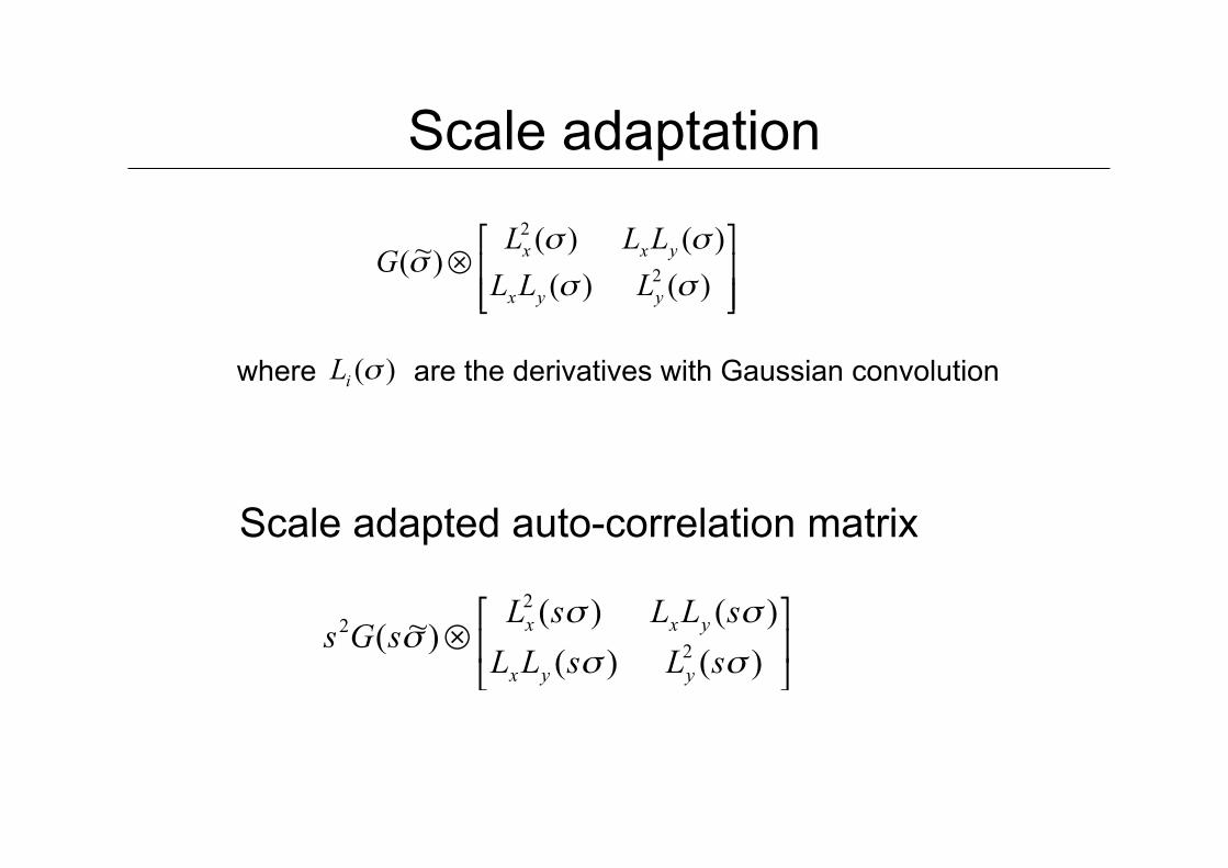
Scale adaptation

Scale adapted auto-correlation matrix

where are the derivatives with Gaussian convolution

Harris detector – adaptation to scale

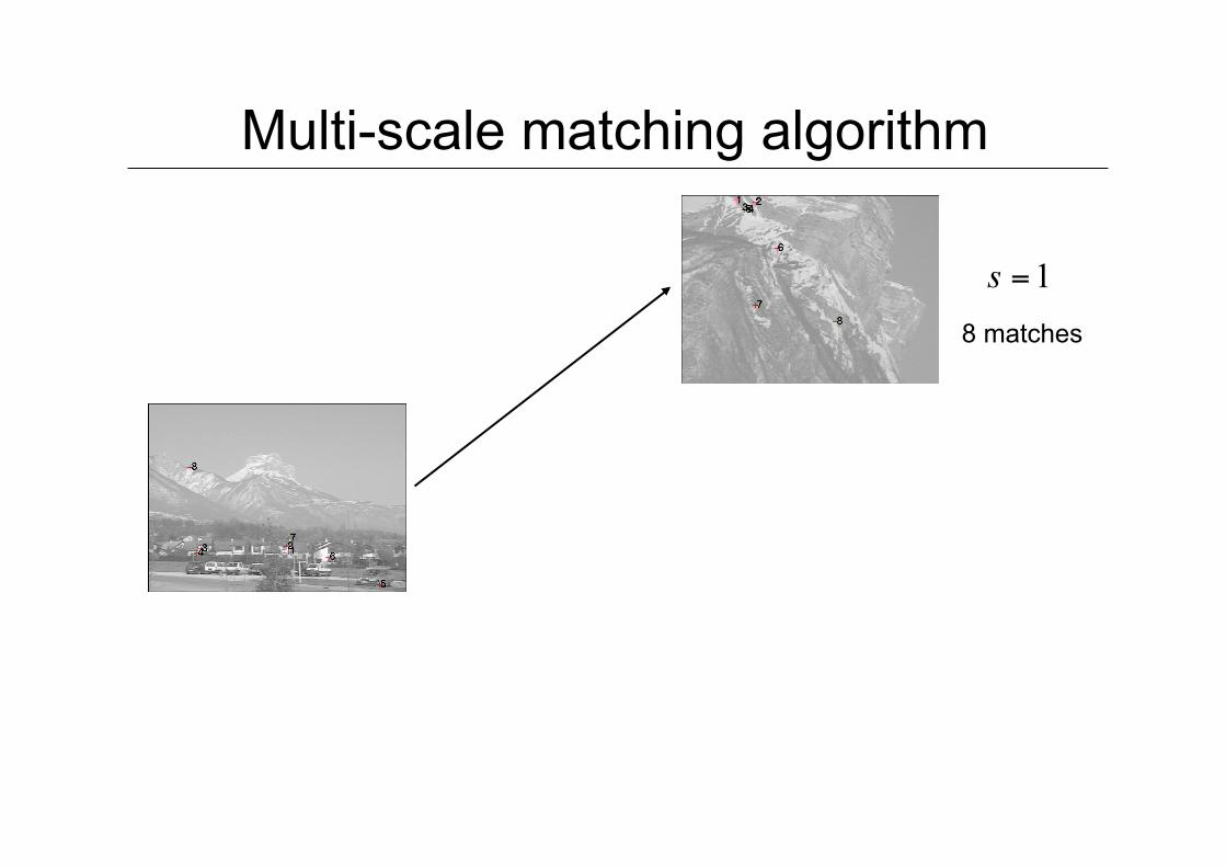
Multi-scale matching algorithm


8 matches


3 matches

Robust estimation of a global affine transformation


4 matches

3 matches


3 matches

4 matches

16 matches correct scale

highest number of matches

Matching results

Scale change of 5.7

Matching results

100% correct matches (13 matches)

Scale selection •  We want to find the characteristic scale by convolving it

with, for example, Laplacians at several scales and looking for the maximum response

•  However, Laplacian response decays as scale increases:

Why does this happen?

increasing σ original signal (radius=8)

Scale normalization

•  The response of a derivative of Gaussian filter to a perfect step edge decreases as σ increases

Scale normalization

•  The response of a derivative of Gaussian filter to a perfect step edge decreases as σ increases

•  To keep response the same (scale-invariant), must multiply Gaussian derivative by σ

•  Laplacian is the second Gaussian derivative, so it must be multiplied by σ2

Effect of scale normalization

Scale-normalized Laplacian response

Unnormalized Laplacian response Original signal

maximum

Blob detection in 2D

•  Laplacian of Gaussian: Circularly symmetric operator for blob detection in 2D

Blob detection in 2D

•  Laplacian of Gaussian: Circularly symmetric operator for blob detection in 2D

Scale-normalized:

Scale selection

•  The 2D Laplacian is given by

•  For a binary circle of radius r, the Laplacian achieves a maximum at

r

image

Lapl

acia

n re

spon

se

scale (σ)

(up to scale)

Characteristic scale

•  We define the characteristic scale as the scale that produces peak of Laplacian response

characteristic scale T. Lindeberg (1998). Feature detection with automatic scale selection.

International Journal of Computer Vision 30 (2): pp 77--116.

Scale selection

•  For a point compute a value (gradient, Laplacian etc.) at several scales

•  Normalization of the values with the scale factor

•  Select scale at the maximum → characteristic scale

•  Exp. results show that the Laplacian gives best results

e.g. Laplacian

scale

Scale selection

•  Scale invariance of the characteristic scale no

rm. L

ap.

s

scale

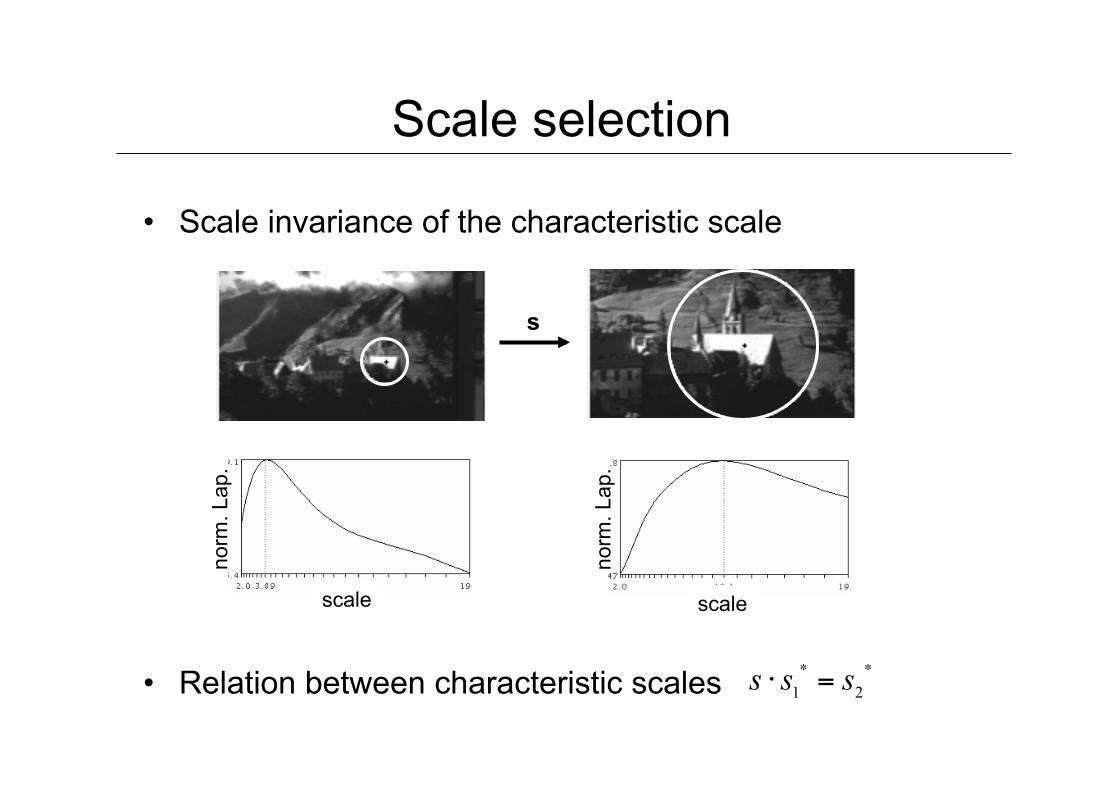
Scale selection

•  Scale invariance of the characteristic scale no

rm. L

ap.

norm

. Lap

.

s

•  Relation between characteristic scales

scale scale

Scale-invariant detectors

•  Harris-Laplace (Mikolajczyk & Schmid’01)

•  Laplacian detector (Lindeberg’98)

•  Difference of Gaussian (Lowe’99)

Harris-Laplace Laplacian

Harris-Laplace

invariant points + associated regions [Mikolajczyk & Schmid’01]

multi-scale Harris points

selection of points at maximum of Laplacian

Matching results

213 / 190 detected interest points

Matching results

58 points are initially matched

Matching results

32 points are matched after verification – all correct

LOG detector

Detection of maxima and minima of Laplacian in scale space

Convolve image with scale-normalized Laplacian at several scales

Efficient implementation •  Difference of Gaussian (DOG) approximates the

Laplacian

•  Error due to the approximation

DOG detector

•  Fast computation, scale space processed one octave at a time

David G. Lowe. "Distinctive image features from scale-invariant keypoints.”IJCV 60 (2).

Local features - overview

•  Scale invariant interest points

•  Affine invariant interest points

•  Evaluation of interest points

•  Descriptors and their evaluation

Affine invariant regions - Motivation

•  Scale invariance is not sufficient for large baseline changes

detected scale invariant region

projected regions, viewpoint changes can locally be approximated by an affine transformation

Affine invariant regions - Motivation

Affine invariant regions - Example

Harris/Hessian/Laplacian-Affine

•  Initialize with scale-invariant Harris/Hessian/Laplacian points

•  Estimation of the affine neighbourhood with the second moment matrix [Lindeberg’94]

•  Apply affine neighbourhood estimation to the scale-invariant interest points [Mikolajczyk & Schmid’02, Schaffalitzky & Zisserman’02]

•  Excellent results in a recent comparison

Affine invariant regions

•  Based on the second moment matrix (Lindeberg’94)

•  Normalization with eigenvalues/eigenvectors

Affine invariant regions

Isotropic neighborhoods related by image rotation

•  Iterative estimation – initial points

Affine invariant regions - Estimation

•  Iterative estimation – iteration #1


•  Iterative estimation – iteration #2


•  Iterative estimation – iteration #3, #4


Harris-Affine versus Harris-Laplace

Harris-Laplace Harris-Affine

Harris-Affine

Hessian-Affine

Harris/Hessian-Affine

Harris-Affine

Hessian-Affine

Matches

22 correct matches

Matches

33 correct matches

Maximally stable extremal regions (MSER) [Matas’02]

•  Extremal regions: connected components in a thresholded image (all pixels above/below a threshold)

•  Maximally stable: minimal change of the component (area) for a change of the threshold, i.e. region remains stable for a change of threshold

•  Excellent results in a recent comparison

Maximally stable extremal regions (MSER)

Examples of thresholded images

high threshold

low threshold

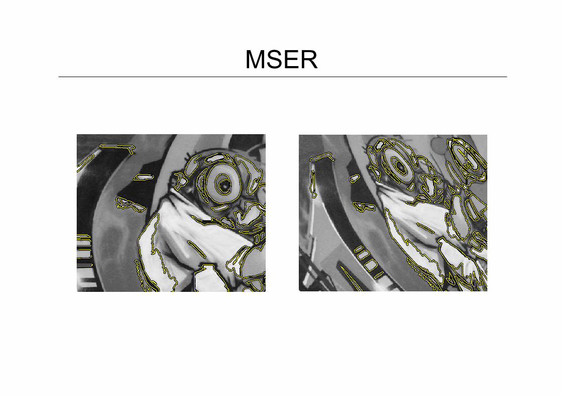
MSER

Overview






Evaluation of interest points

•  Quantitative evaluation of interest point/region detectors –  points / regions at the same relative location and area

•  Repeatability rate : percentage of corresponding points

•  Two points/regions are corresponding if –  location error small –  area intersection large

•  [K. Mikolajczyk, T. Tuytelaars, C. Schmid, A. Zisserman, J. Matas, F. Schaffalitzky, T. Kadir & L. Van Gool ’05]

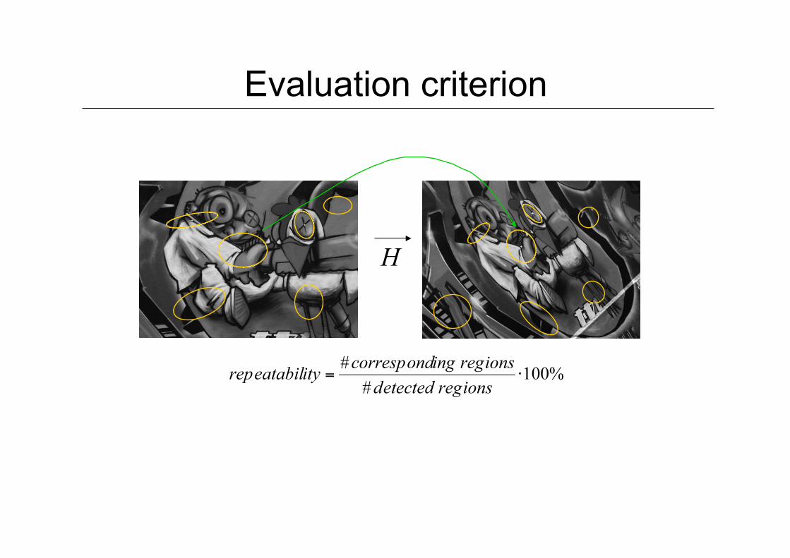
Evaluation criterion

H

Evaluation criterion

H

2% 10% 20% 30% 40% 50% 60%

Dataset

•  Different types of transformation –  Viewpoint change –  Scale change –  Image blur –  JPEG compression –  Light change

•  Two scene types –  Structured –  Textured

•  Transformations within the sequence (homographies) –  Independent estimation

Viewpoint change (0-60 degrees )

structuredscene

texturedscene

Zoom + rotation (zoom of 1-4)

structuredscene

texturedscene

Blur, compression, illumination

blur-structuredscene blur-texturedscene

lightchange-structuredscene jpegcompression-structuredscene

Comparison of affine invariant detectors

!"#$#"%$%"&$&""$""'$'"$!$#$%$&$"$'$($)$*$!$$+,-./0,1234156-7-/-4248,6,293:;477,<!=>>,1-;-<<,41!=>>,1-?@ABCDBADB@46,-12

!"#$#"%$%"&$&""$""'$'"$#$$&$$'$$($$!$$$!#$$!&$$)*+,-.*/012/34+/567+81.91:.88+;-./<+/:+;=288*;!>99*/+=+;;*2/!>99*/+?@ABCDBADB@24*+/0

Viewpoint change - structured scene repeatability % # correspondences

reference image 20 60 40

Scale change repeatability % repeatability %

reference image 4 reference image 2.8

Comparison of affine invariant detectors

•  Good performance for large viewpoint and scale changes

•  Results depend on transformation and scene type, no one best detector

•  Detectors are complementary –  MSER adapted to structured scenes –  Harris and Hessian adapted to textured scenes

•  Performance of the different scale invariant detectors is very similar (Harris-Laplace, Hessian, LoG and DOG)

•  Scale-invariant detector sufficient up to 40 degrees of viewpoint change

Conclusion - detectors

Overview






Region descriptors

•  Normalized regions are –  invariant to geometric transformations except rotation –  not invariant to photometric transformations

Descriptors

•  Regions invariant to geometric transformations except rotation –  normalization with dominant gradient direction

•  Regions not invariant to photometric transformations –  normalization with mean and standard deviation of the image patch

Descriptors

Extract affine regions Normalize regions Eliminate rotational

+ illumination Compute appearance

descriptors

SIFT (Lowe ’04)

Descriptors

•  Gaussian derivative-based descriptors –  Differential invariants (Koenderink and van Doorn’87) –  Steerable filters (Freeman and Adelson’91)

•  Moment invariants [Van Gool et al.’96]

•  SIFT (Lowe’99) •  Shape context [Belongie et al.’02]

•  SIFT with PCA dimensionality reduction •  Gradient PCA [Ke and Sukthankar’04]

•  SURF descriptor [Bay et al.’08]

•  DAISY descriptor [Tola et al.’08, Windler et al’09]

Comparison criterion •  Descriptors should be

–  Distinctive –  Robust to changes on viewing conditions as well as to errors of

the detector

•  Detection rate (recall) –  #correct matches / #correspondences

•  False positive rate –  #false matches / #all matches

•  Variation of the distance threshold –  distance (d1, d2) < threshold

1

1

[K. Mikolajczyk & C. Schmid, PAMI’05]

Viewpoint change (60 degrees)

!!"#!"$!"%!"&!"'!"(!")!"*!"+#!!"#!"$!"%!"&!"'!"(!")!"*!"+##!,-./010234/2--./5676$#!#

esift * * shape context

gradient pca

cross correlation

complex filters

!"#!"$$%&'($)

steerable filters

gradient moments

sift

esift * *

Scale change (factor 2.8)

!!"#!"$!"%!"&!"'!"(!")!"*!"+#!!"#!"$!"%!"&!"'!"(!")!"*!"+##!,-./010234/2--./5676$!*(

shape context

gradient pca

cross correlation

complex filters

!"#!"$$%&'($)

steerable filters

gradient moments

sift

Conclusion - descriptors

•  SIFT based descriptors perform best

•  Significant difference between SIFT and low dimension descriptors as well as cross-correlation

•  Robust region descriptors better than point-wise descriptors

•  Performance of the descriptor is relatively independent of the detector

Available on the internet

•  Binaries for detectors and descriptors –  Building blocks for recognition systems

•  Carefully designed test setup –  Dataset with transformations –  Evaluation code in matlab –  Benchmark for new detectors and descriptors

http://lear.inrialpes.fr/software

Documents

Overview - École normale supérieure de Lyon · Overview • Harris ... • Estimation of the affine neighbourhood with the second moment matrix ... Blur, compression, illumination