Embed Size (px)
Citation preview
American Economic Review 101 (December 2011): 3400–3426http://www.aeaweb.org/articles.php?doi=10.1257/aer.101.7.3400
3400
In the wake of the 2008 international financial crisis, there have been intense debates about reform of the international financial system that emphasize the need to address the problem of “overborrowing.” The argument typically relies on the observation that periods of sustained increases in borrowing are often followed by a devastating disruption in financial markets. This raises the question of why the private sector becomes exposed to the dire consequences of financial crises and what the appropriate policy response should be to reduce the vulnerability to these epi-sodes. Without a thorough understanding of the underlying inefficiencies that arise in the financial sector, it seems difficult to evaluate the merit of proposals that aim to reform the current international financial architecture.
This article presents a formal welfare-based analysis of how optimal borrow-ing decisions at the individual level can lead to overborrowing at the social level in a dynamic stochastic general equilibrium (DSGE) model, where financial con-straints give rise to amplification effects. As in the theoretical literature (e.g. Guido Lorenzoni 2008), we analyze constrained efficiency by considering a social planner that faces the same financial constraints as the private economy, but internalizes the price effects of its borrowing decisions. Unlike the existing literature, we conduct a quantitative analysis to evaluate the macroeconomic and welfare effects of overbor-rowing. We study how overborrowing affects the incidence and severity of financial crises, the magnitude of welfare losses, and the features of policy measures that aim to correct the externality. In a nutshell, we investigate whether overborrowing is in fact a macroeconomic problem and what should be the optimal policy response.
Our model’s key feature is an occasionally binding credit constraint that limits borrowing, denominated in the international unit of account (i.e., tradable goods), to the value of collateral in the form of output from the tradable and nontradable sec-tor, as in Enrique G. Mendoza (2002). Because debt is partially leveraged in income generated in the nontradable sector, changes in the relative price of nontradable goods can induce sharp and sudden adjustments in access to foreign financing. Due to incomplete markets, agents can only imperfectly insure against adverse shocks. As a result, when agents have accumulated a large amount of debt and a typical
Overborrowing and Systemic Externalities in the Business Cycle†
By Javier Bianchi*
* Department of Economics, New York University, 19 West 4th Street, New York, NY 10012, and University of Wisconsin-Madison (e-mail: [email protected]). This paper is based on my dissertation at the University of Maryland. I am indebted to my advisors Enrique Mendoza, Anton Korinek, Carlos Vegh, and John Shea. For use-ful comments and suggestions, I thank three anonymous referrees, V. V. Chari, Pablo D’Erasmo, Juan Dubra, Bora Durdu, Emmanuel Farhi, Bertrand Gruss, Tim Kehoe, Alessandro Rebucci, Carmen Reinhart, Horacio Sapriza, and participants at several seminars and conferences. I am grateful to the Federal Reserve Bank of Atlanta and the Board of Governors of the Federal Reserve for their hospitality.
† To view additional materials, visit the article page at http://www.aeaweb.org/articles.php?doi=10.1257/aer.101.7.3400.
3401BiAnchi: OvERBORROwing AnD SyStEmic ExtERnAlitiESvOl. 101 nO. 7
adverse shock hits, the economy suffers the typical dislocation associated with an emerging market crisis. Demand for consumption goods falls, putting downward pressure on the price of nontradables, which drags down the real exchange rate. This leads to a further tightening of the credit constraint, setting in motion Fisher’s debt deflation channel by which declines in consumption, the real exchange rate, and access to foreign financing mutually reinforce one another, as in Mendoza’s work.
In the model, private agents form rational expectations about the evolution of mac-roeconomic variables—in particular the real exchange rate—and correctly perceive the risks and benefits of their borrowing decisions. Nevertheless, they fail to inter-nalize the general equilibrium effects of their borrowing decisions on prices. This is a pecuniary externality that would not impede market efficiency in the absence of the credit constraint linked to market prices. However, by reducing the amount of borrowing ex ante, a social planner mitigates the decrease in demand for consump-tion during crises. This mitigates the real exchange rate depreciation and prevents a further tightening of financial constraints, making everyone better off.
Our quantitative analysis shows that the macroeconomic effects of the systemic credit externality are significant. The externality increases the long-run probability of a financial crisis from 0.4 percent to 5.5 percent and has important effects on the severity of these episodes. In the decentralized equilibrium, consumption drops 17 percent, capital inflows fall 8 percent, and the real exchange rate drops by 19 percent in a typical crisis. In the constrained-efficient allocations, by contrast, con-sumption drops 10 percent, capital inflows barely fall, and the real exchange rate drops by 1 percent. Moreover, the externality allows the model to account for two salient features of the data: procyclicality of capital inflows and the high variability of consumption.
We study a variety of policy measures that can restore constrained efficiency, all of which involve restricting the amount of credit in the economy: taxes on debt, tightening of margins, and capital and liquidity requirements. These measures are imposed before a crisis hits so that private agents internalize the external costs of borrowing and the economy becomes less vulnerable to future adverse shocks. In the calibrated version of our model, the increase in the effective cost of borrowing necessary to implement the constrained-efficient allocations is about 5 percent on average, increasing with the level of debt and with the probability of a future finan-cial crisis. We also study simple forms of interventions and ascertain that a fixed tax on debt can also achieve sizable welfare gains.
Our article is related to the large literature on the macroeconomic role of finan-cial frictions. Following the work of Ben Bernanke and Mark Gertler (1989) and Nobuhiro Kiyotaki and John Moore (1997), various studies have presented dynamic models where financial frictions can amplify macroeconomic shocks compared to a first-best benchmark where these frictions are absent.1 Our contribution to this literature is twofold. First, we study the volatility and the level of amplification of the competitive equilibrium relative to a second-best benchmark where these frictions are also present. Second, we investigate several policy measures that can
1 See, for example, Rao Aiyagari and Gertler (1999), Bernanke, Gertler, and Simon Gilchrist (1999), Matteo Iacoviello (2005), Gertler, Gilchrist, and Fabio Natalucci (2007), and Mendoza (2002, 2010).
3402 thE AmERicAn EcOnOmic REviEw DEcEmBER 2011
significantly reduce the level of financial instability and improve welfare by making agents internalize an externality due to financial accelerator effects.
Our article is related to the theoretical literature that investigates the role of pecu-niary externalities in generating excessive financial fragility, and we borrow exten-sively from their insights (see, for example, Leonardo Auernheimer and Roberto Garcia-Saltos 2000; Ricardo Caballero and Arvind Krishnamurthy 2001, 2003; Lorenzoni 2008; Emmanuel Farhi, Mikhail Golosov, and Aleh Tsyvinski 2009; and Anton Korinek 2009a, b).2 In all of these studies, however, the analysis is qualitative in nature. Our contribution to this literature is to provide a quantitative assessment of the macroeconomic, policy, and welfare implications of overborrowing. This is an important first step in the evaluation of the potential benefits from regulatory mea-sures to correct these externalities and in the study of their practical implementation.
There is a growing macroeconomic literature that studies optimal policy in a financial crisis.3 This literature typically takes as given that the economy is in a high leverage situation and analyzes the role of policies that can moderate the impact of a large adverse shock. While this literature provides important insights on how to respond to crises once they erupt, it does not study how the economy experiences the surge in debt that leads to the crisis in the first place. This article complements this literature by studying how an economy can become vulnerable to a financial crisis due to excessive borrowing during normal times. We model crises as infrequent episodes nested within regular business cycles and analyze the role of policies in reducing an economy’s vulnerability to financial crises, therefore placing macro-prudential policy at the center of the stage. We acknowledge, however, that because our analysis requires global nonlinear solution methods, we abstract from important real-world features present in larger scale DSGE models.
A related article that allows for policy intervention during normal times and crisis times is Benigno et al. (2009). They consider the role of a subsidy on nontradable goods, which the Ramsey planner uses ex post to mitigate the real exchange depre-ciation during crises, but not ex ante since it is not effective to make agents internal-ize the full social costs of borrowing. We focus instead on a constrained planner who directly makes borrowing decisions and show that the decentralization requires ex ante intervention to prevent excessive risk exposure.
Finally, there are a number of other theories of overborrowing that have been investigated. One theory is moral hazard: banks may lend excessively to take advan-tage of some form of government bailout.4 Martin Uribe (2006) has also studied whether an economy with an aggregate debt limit tends to overborrow relative to an economy with debt limits imposed at the level of each individual agent and found that borrowing decisions coincide. Our focus is on the comparison between compet-itive equilibrium and constrained-efficient equilibrium when financial constraints that are linked to market prices generate amplification effects.
2 The inefficiency result of these studies is related to the idea that economies with endogenous borrowing con-straints and multiple goods can be constrained inefficient (Tim Kehoe and David Levine 1993) and to the generic inefficiency result in economies with incomplete markets (John Geanakoplos and Heraklis Polemarchakis 1986; Joseph Stiglitz 1982).
3 Notable contributions include Lawrence Christiano, Christopher Gust, and Jorge Roldos (2004); Kiyotaki and Moore (2008); Gertler and Peter Karadi (2009); and Gertler and Kiyotaki (2010).
4 See, e.g., Ronald McKinnon and Huw Pill (1996); Giancarlo Corsetti, Paolo Pesenti, and Nouriel Roubini (1999); Martin Schneider and Aaron Tornell (2004); and Farhi and Jean Tirole (forthcoming).
3403BiAnchi: OvERBORROwing AnD SyStEmic ExtERnAlitiESvOl. 101 nO. 7
I. Analytical Framework
Consider a representative-agent DSGE model of a small open economy (SOE) with a tradable goods sector and a nontradable goods sector. Only tradable goods can be traded internationally; nontradable goods have to be consumed in the domes-tic economy. The economy is populated by a continuum of identical, infinitely-lived households of measure unity with preferences given by:
(1) 피 0 { ∑ t=0
∞
β t u( c t )} .
In this expression, 피 t ( ⋅ ) is the time t expectation operator, and β is the discount factor. The period utility function u( ⋅ ) has the constant-relative-risk-aversion (CRRA) form. The consumption basket c t is an Armington-type CES aggregator with elasticity of substitution 1/(η + 1) between tradable c t and nontradable goods c n given by:
c t = [ω( c t t )
−η + (1 − ω) ( c t n )
−η ] − 1 _ η , η > −1, ω ∈ (0, 1).
In each period t, households receive an endowment of tradable goods y t t and an
endowment of nontradable goods y t n . We assume that the vector of endowments
given by y ≡ ( y t , y n ) ∈ y ⊆ R ++ 2 follows a first-order Markov process. These
endowment shocks are the only source of uncertainty in the model.The menu of foreign assets available is restricted to a one period, non–state con-
tingent bond denominated in units of tradables that pays a fixed interest rate r, deter-mined exogenously in the world market.5 Normalizing the price of tradables to 1 and denoting the price of nontradable goods by p n the budget constraint is:
(2) b t+1 + c t t + p t
n c t n = b t (1 + r) + y t
t + p t n y t
n ,
where b t+1 denotes bond holdings that households choose at the beginning of time t. We maintain the convention that positive values of b denote assets. As there is only one asset, gross and net bond holdings (NFA) coincide.
We assume that creditors restrict loans so that the amount of debt does not exceed a fraction κ t of tradable income and a fraction κ n of nontradable income. Specifically, the credit constraint is given by:
(3) b t+1 ≥ − ( κ n p t n y t
n + κ t y t t ).
5 To have a well-defined stochastic steady state, we assume that the discount factor and the world interest rate are such that β(1 + r) < 1. If β(1 + r) ≥ 1, assets will diverge to infinity in equilibrium by the supermartingale convergence theorem (see Gary Chamberlain and Charles Wilson 2000). See Stephanie Schmitt-Grohe and Uribe (2003) for other methods to induce stationarity.
3404 thE AmERicAn EcOnOmic REviEw DEcEmBER 2011
This credit constraint can be seen as arising from informational and institutional frictions affecting credit relationships (such as monitoring costs, limited enforce-ment, asymmetric information, and imperfections in the judicial system), but we do not model these frictions explicitly. Our focus is on how financial policies can be welfare improving, taking as given the frictions that lead to these debt contracts, i.e., we will assume that the social planner is a constrained social planner that is also subject to this credit constraint.
Discussion of market incompleteness.—A few comments are in order about the two deviations from complete markets that we introduce here. First, we have assumed that assets are restricted to a one-period non–state contingent bond denom-inated in tradable goods. While agents typically have a richer set of assets avail-able, this assumption is made for numerical tractability and is meant to capture the observation that debt in emerging markets is generally short term and denominated in foreign currency. In turn, these features of debt contracts are generally seen as an important source of vulnerability in emerging markets (see, e.g., Guillermo A. Calvo, Alejandro Izquierdo, and Rudy Loo-Kung 2006).
The second form of market incompleteness is given by the credit constraint. In the absence of a credit constraint, households will increase borrowing in bad times to smooth consumption. This will imply a counterfactual reaction of the current account, which is well known to rise during recessions in emerging markets. The credit constraint we have specified has two main features. One crucial feature is that nontradable goods are part of the collateral. At the empirical level, this is consistent with evidence that credit booms in the nontradable sector are fueled by external credit (see, e.g., Tornell and Frank Westermann 2005). At the theoretical level, this could result because foreign borrowers can seize nontradable goods from a defaulting borrower, sell them in the domestic market, and repatriate the funds abroad. A positive gap between κ t and κ n would reflect an environment where creditors have a higher preference for tradable income as collateral. A case where κ t = κ n would reflect an environment where creditors request and aim to verify information on total income of individual borrowers, i.e., they do not docu-ment the sectoral sources of their income.
The second feature is that the collateral is given by current income. At the empiri-cal level, this assumption is supported by evidence that current income is a major determinant of credit market access (see, e.g., Tullio Jappelli 1990).6 At the theoreti-cal level, this could be the outcome of an environment where households can divert all future income in the period they contract debt obligations. Further, if creditors detect the fraud and can seize a fraction of the household’s current income, they would impose a credit limit according to the level of current income (see Korinek 2009a).
An additional argument that our formulation of the credit constraint is suitable for a quantitative assessment of the externality is that our model can account rea-sonably well for the main macro features of emerging market crises, as shown by Mendoza (2002).
6 For more evidence on credit constraints on households, see Jappelli and Marco Pagano (1989); Steve Zeldes (1989).
3405BiAnchi: OvERBORROwing AnD SyStEmic ExtERnAlitiESvOl. 101 nO. 7
II. Equilibrium
A. Optimality conditions
The household’s problem is to choose stochastic processes { c t t , c t
n , b t+1 } t≥0 to max-imize the expected present discounted value of utility (1) subject to (2) and (3), tak-ing b 0 and { p t
n } t≥0 as given. The household’s first-order conditions require:
(4) λ t = u t (t)
(5) p t n = ( 1 − ω _ ω )( c t
t _ c t
n )
η+1
(6) λ t = β(1 + r) 피 t λ t+1 + μ t
(7) b t+1 + ( κ n p t n y t
n + κ t y t t ) ≥ 0, with equality if μ t > 0,
where λ is the nonnegative multiplier associated with the budget constraint and μ is the nonnegative multiplier associated with the credit constraint. The optimality con-dition (4) equates the marginal utility of tradable consumption to the shadow value of current wealth. Condition (5) equates the marginal rate of substitution of the two goods, tradables and nontradables, to their relative price. Equation (6) is the Euler equation for bonds. When the credit constraint is binding, there is a wedge between the current shadow value of wealth and the expected value of reallocating wealth to the next period, given by the shadow price of relaxing the credit constraint μ t . Equation (7) is the complementary slackness condition.
Since households are identical, market clearing conditions are given by:
(8) c t n = y t
n
(9) c t t = y t
t + b t (1 + r) − b t+1 .
Notice that equation (5) implies that a reduction in c t t generates in equilibrium a
reduction in p t n , which by equation (3) reduces the collateral value. Besides ampli-
fication, the credit constraint produces asymmetric responses in the economy: a binding credit constraint amplifies the consumption drop in response to a negative income shock, but no amplification effects occur when the credit constraint is slack. Because of consumption-smoothing effects, the demand for borrowing generally decreases with current income, and when current income is sufficiently low, the credit constraint becomes binding.
B. Equilibrium Definition
We consider the optimization problem of a representative household in recur-sive form, which includes, as a crucial state variable, the aggregate bond hold-ings of the economy. Households need to forecast future aggregate bond holdings that are beyond their control to form expectations of the price of nontradables. We
3406 thE AmERicAn EcOnOmic REviEw DEcEmBER 2011
denote by Γ( ⋅ ) the forecast of aggregate bond holdings for every current aggregate state (B, y), i.e., B′ = Γ(B, y). Combining equilibrium conditions (5), (8), and (9), the forecast price function for nontradables can be expressed as p n (B, y) = (1 − ω)/(ω) (( y t + B(1 + r) − Γ(B, y))/ y n ) η+1 . The other relevant state variables for the individual household are its bond holdings and the vector of endowment shocks. The problem of a representative household can then be written as:
(10) v(b, B, y) = max b′, c t , c n
u(c( c t , c n )) + β 피 y′ | y v(b′, B′, y′ )
subject to
b′ + p n (B, y) c n + c t = y t + b(1 + r) + p n (B, y) y n
b′ ≥ − ( κ n p n (B, y) y n + κ t y t )
B′ = Γ(B, y),
where we have followed the convention of denoting current variables without sub-script and denoting next period variables with the prime superscript. The solu-tion to the household problem yields decision rules for individual bond holdings b (b, B, y), tradable consumption c t (b, B, y) and nontradable consumption c n (b, B, y). The household optimization problem induces a mapping from the perceived law of motion for aggregate bond holdings to an actual law of motion, given by the repre-sentative agent’s choice b (b, B, y). In a rational expectations equilibrium, as defined below, these two laws of motion must coincide.
DEFINITION 1: (Decentralized Recursive competitive Equilibrium) A decentral-ized recursive competitive equilibrium for our SOE is defined by a pricing func-tion p n (B, y), a perceived law of motion Γ(B, y), and decision rules { b (b, B, y), c t (b, B, y), c n (b, B, y)} with associated value function v(b, B, y) such that the follow-ing conditions hold:
(i) household optimization: { b (b, B, y), c n (b, B, y), c n (b, B, y), v (b, B, y)} solve the recursive optimization problem of the household for given p n (B, y) and Γ(B, y).
(ii) Rational expectation condition: the perceived law of motion is consistent with the actual law of motion: Γ(B, y) = b (b, B, y).
(iii) markets clear: y n = c n (b, B, y) and Γ(B, y) + c t (b, B, y) = y t + B(1 + r).
III. Efficiency
A. Social Planner’s Problem
We previously described the equilibrium achieved when agents take aggregate variables as given, particularly the price of nontradables. Consider now a benevolent social planner with restricted planning abilities. We assume that the social planner
3407BiAnchi: OvERBORROwing AnD SyStEmic ExtERnAlitiESvOl. 101 nO. 7
can directly choose the level of debt subject to the credit constraint but allows goods markets to clear competitively. That is, the planner (a) performs credit operations and rebates back to households all the proceeds in a lump sum fashion, and (b) lets households choose their allocation of consumption between tradable goods and non-tradable goods in a competitive way.
As opposed to the representative agent, a social planner internalizes the effects of borrowing decisions on the price of nontradables. Critically, the social planner realizes that a lower debt level mitigates the reduction in the price of nontradables and prevents a larger drop in borrowing ability when the credit constraint binds. As a result, we will show that the decentralized equilibrium allocation is not a con-strained Pareto optimum, as defined below.
DEFINITION 2: (constrained Efficiency) let { c t t , c t
n , b t+1 } t≥0 be the allocations of the competitive equilibrium yielding utility v . the competitive equilibrium is con-strained efficient if a social planner that chooses directly { b t+1 } t≥0 subject to the credit constraint, but lets the goods markets clear competitively, cannot improve the welfare of households above v .
The social planner’s optimization problem consists of maximizing (1) subject to (3), (5), (8), and (9). Substituting for the equilibrium price in (3), we can express the social planner’s optimization problem in recursive form as:
(11) v(b, y) = max b′, c t
u(c( c t , y n )) + β 피 y′ | y v(b′, y′ )
subject to
b′ + c t = y t + b(1 + r)
b′ ≥ −( κ n 1 − ω _ ω ( c t _ y n )
η+1
y n + κ t y t ).
Using sequential notation and the superscript “sp” to distinguish the Lagrange mul-tipliers of the social planner’s problem from the decentralized equilibrium, the first-order conditions for the social planner require:
(12) λ t sp = u t (t) + μ t
sp Ψ t
(13) λ t sp = β(1 + r) 피 t λ t+1
sp + μ t
sp
(14) b t+1 + ( κ n 1 − ω _ ω ( c t _ y t n )
η+1
y t n + κ t y t
t ) ≥ 0, with equality if μ t sp > 0,
where Ψ t ≡ κ n ( p t n c t
n )/( c t t )(1 + η) > 0 indicates how much the collateral value
changes at equilibrium when there is a change in tradable consumption. Notice that this term is directly proportional to the fraction of nontradable output that agents can pledge as collateral, the relative size of the nontradable sector, and the inverse of the
3408 thE AmERicAn EcOnOmic REviEw DEcEmBER 2011
elasticity of substitution between tradables and nontradables. We will return to this expression in the sensitivity analysis.
The key difference between the optimization problem of the social planner rela-tive to households follows from examining (12) compared with the correspond-ing equation for the decentralized equilibrium (4). The social planner’s marginal benefits from tradable consumption include the direct increase in utility u t (t) and also the indirect increase in utility μ t
sp Ψ t . This indirect benefit, not considered by private agents, represents how an increase in tradable consumption increases the price of nontradables and relaxes the credit constraint of all agents by Ψ t , which has a shadow value of μ t
sp . Thus, (4) and (12) yield the key result that, for given initial states and allocations at which the credit constraint binds, private agents value wealth less than the social planner, which we highlight in the following remark.
REMARK 1: when the credit constraint binds, private agents undervalue wealth.
To see more clearly why this different ex post valuation generates overborrowing ex ante, suppose that at time t the constraint is not currently binding. Using (4) and (6), the Euler equation for consumption in the decentralized equilibrium becomes:
(15) u t (t) = β(1 + r) 피 t u t (t + 1).
Using (12) and (13), the Euler equation for consumption for the social planner becomes:
(16) u t (t) = β(1 + r) 피 t [u t (t + 1) + μ t+1 sp
Ψ t+1 ] .
Consider now a reallocation of wealth by the social planner starting from the pri-vately optimal allocations in the decentralized equilibrium. In particular, consider the welfare effects of a reduction of one unit of borrowing. Because decentralized agents are at the optimum, (15) shows that the first-order private welfare benefits β(1 + r) E t u t (t + 1) are equal to the first-order private welfare costs u t (t). Using (16), the social planner has a marginal cost of reducing borrowing equal to the private marginal cost but faces higher marginal benefits: a one unit decrease in bor-rowing relaxes next-period ability to borrow by (1 + r) Ψ t+1 , which has a marginal utility benefit of μ t+1
sp . The uninternalized external benefits from savings, or equiva-
lently the uninternalized external marginal cost of borrowing, is then given by the discounted expected marginal utility cost of the resulting tightening of the credit constraint β(1 + r) 피 t μ t+1
sp Ψ t+1 . Notice that if the credit constraint does not bind for
any pair (b, y) in the two equilibria, the conditions characterizing both environments are identical, and therefore the allocations coincide.
PROPOSITION 1: (constrained inefficiency) the decentralized equilibrium is not, in general, constrained efficient.
PROOF:See Appendix A.
3409BiAnchi: OvERBORROwing AnD SyStEmic ExtERnAlitiESvOl. 101 nO. 7
B. Decentralization
We study the use of various financial policies in the implementation of the con-strained-efficient allocations. We start by showing how a tax on debt can restore con-strained efficiency and then show the equivalence between the tax on debt and more standard forms of intervention in the financial sector (e.g., capital requirements).
Letting τ t be the tax charged on debt issued at time t, the Euler equation for bonds in the regulated decentralized equilibrium (6) becomes:
(17) u t (t) = β(1 + r)(1 + τ t ) 피 t u t (t + 1) + μ t .
PROPOSITION 2: (Optimal tax on debt) the constrained-efficient allocations can be implemented with an appropriate state contingent tax on debt, with tax revenue rebated as a lump sum transfer.
PROOF:See Appendix A.
When the credit constraint is not binding in the constrained-efficient allocations, the tax must be set to τ t * = ( 피 t μ t+1
sp Ψ t+1 )/( 피 t u t (t + 1)) (variables are evaluated at
the constrained-efficient allocations). This expression represents the uninternalized marginal cost of borrowing analyzed above, normalized by the expected marginal utility. As we will see in the quantitative analysis, this tax increases with the current level of debt, since a higher current level of debt implies a higher choice of debt, which increases the probability and the marginal utility cost of a binding constraint next period. Notice also that if the credit constraint has a zero probability of being binding in the next period, the tax is set to zero.
When the credit constraint is binding, the tax does not generally influence the level of borrowing, since the choice of debt is given by the credit constraint (3) and not by the Euler equation (17). Setting the tax to τ t * = ( 피 t μ t+1
sp Ψ t+1 )/( 피 t u t (t + 1)) −
( μ t sp Ψ t )(β(1 + r) 피 t u t (t + 1)) achieves constrained efficiency and equalizes the pri-
vate and social shadow values from relaxing the constraint. Notice that an extra term arises because the social planner internalizes that relaxing the credit constraint today would have positive effects on the current price of nontradables. This term is nega-tive so that the tax causes the private shadow value of relaxing the constraint to rise to the social value. As we will show in the quantitative analysis, when the planner is borrowing up to the limit, the level of borrowing desired by private agents is also the maximum available. As a result, we find that setting τ t * = 0 when the constraint binds also implements the constrained-efficient allocations, and since this results in a sim-pler policy we set this tax to zero when we turn to describe its quantitative features.7
In practice, much of prudential financial regulation is implemented through banks. To take this into consideration, we develop in Appendix B a simple model of finan-cial intermediaries and show that our benchmark economy, in which the planner sets a tax on debt on borrowers, is equivalent to a economy where the planner sets
7 This result held for the wide range of parameters explored in our quantitative analysis.
3410 thE AmERicAn EcOnOmic REviEw DEcEmBER 2011
capital requirements or reserve requirements on financial institutions. Throughout the paper, we will refer to the implied tax on debt as the increase in the cost of debt induced by the use of any of these equivalent policy measures.
Alternatively, the planner could implement the constrained-efficient allocations using margin requirements by choosing an adjustment θ t ≥ 0 such that the credit constraint becomes b t+1 ≥ − (1 − θ t )( κ n p t
n y t n + κ t y t
t ). If the socially optimal amount of borrowing is b t
sp , by setting θ t * = 1 − ( b t sp )/( κ n p t
n y t n + κ t y t
t ) the social planner can restrict the quantity of borrowing and restore constrained efficiency.8
REMARK 2: (Decentralization) the constrained-efficient allocations can be imple-mented with appropriate capital requirements, reserve requirements, or margin requirements.
IV. Quantitative Analysis
In this section, we describe the calibration of the model and evaluate the quantita-tive implications of the externality. We solve for the competitive equilibrium and the constrained-efficient allocations numerically using global nonlinear methods (described in detail in the online Appendix).
A. calibration
The values assigned to all models’ parameters are listed in Table 1. A period in the model represents a year. The baseline calibration uses data from Argentina, an example of an emerging market with a business cycle that has been studied exten-sively. The risk aversion is set at σ = 2, a standard value. The interest rate is set at r = 4 percent, which is a standard value for the world risk-free interest rate in the DSGE-SOE literature.
We model endowment shocks as a first-order bivariate autoregressive process: log yt = ρ log y t−1 + ε t where y = [ y t y n ]′, ρ is a 2x2 matrix of autocorrelation coefficients, and ε t = [ ε t
t ε t n ]′ follows a bivariate normal distribution with zero
mean and contemporaneous variance-covariance matrix V. This process is estimated with the HP-filtered cyclical components of tradables and nontradables GDP from the World Development Indicators (WDI) for the 1965–2007 period, the longest time series available from official sources. Following the standard methodology, we classify manufacturing and primary products as tradables and classify the rest of the components of GDP as nontradables. The estimates of ρ and V are:
ρ = [ 0.901 0.495 − 0.453 0.225
] V = [ 0.00219 0.00162 0.00162 0.00167
] .
8 For this policy to restore constrained efficiency, it must be the case that b de (B, B, y) ≤ b sp
(B, y) ∀ (B, y), which we will show is the case in the numerical analysis. We assume for simplicity that θ * is such that the credit constraint always holds with equality in the regulated economy. In the regulated economy where the adjustment of margins is given by θ * , the constraint binds only in the constrained region and in the tax region; hence, setting θ t = 0 when the constraint does not bind in the constrained-efficient allocations and the optimal tax on debt is zero delivers the same allocations.
3411BiAnchi: OvERBORROwing AnD SyStEmic ExtERnAlitiESvOl. 101 nO. 7
The standard deviations of tradable and nontradable output in the data are σ y t = 0.058 and σ y n = 0.057, the first-order autocorrelations are ρ y t = 0.53 and ρ y n = 0.61, and the correlation between the two is ρ y t , y n = 0.81. Thus, cyclical fluctuations in the two sectors have similar volatility and persistence and are posi-tively correlated with each other. We discretize the vector of shocks into a first-order Markov process, with four grid points for each shock, using the quadrature-based procedure of George Tauchen and Robert Hussey (1991). The mean of the endow-ments is set to one without loss of generality.
The intratemporal elasticity of substitution 1/(η + 1) is a crucial parameter because it affects the magnitudes of the price adjustment. For a given reduction in tradable consumption, a higher elasticity implies a smaller change in the price of nontradables, and therefore we should expect weaker effects from the externality. The range of esti-mates for the elasticity of substitution is between 0.40 and 0.83.9 As a conservative benchmark, we set η such that the elasticity of substitution equals the upper bound of this range and then show how the externality changes with this parameter.
The ratio κ n / κ t determines the relative quality of nontradable and tradable output as collateral. It is difficult, however, to derive a direct mapping from the data to this ratio. We therefore take a pragmatic approach: we begin by setting κ n = κ t and then perform extensive sensitivity analysis.
The three remaining parameters are { β, ω, κ t }, which are set so that the long-run moments of the decentralized equilibrium match three historical moments of the data. The parameter ω governs the tradable share in the CES aggregator and is calibrated to match a 32 percent share of tradable production.10 This approach is a reasonable one to calibrate ω since given the relative endowment and consumption ratios, ω deter-mines the equilibrium price of nontradables by (5) and the share of tradables in the total value of production. This calibration results in a value of ω of 0.32.
The discount factor β is set so that the average net foreign asset position-to-GDP ratio in the model equals its historical average in Argentina, which is equal to −29 percent in the dataset constructed by Philip Lane and Gian Maria Milesi-Ferretti (2001). This calibration results in a value of β = 0.91, a relatively standard value for annual frequency in the literature.
9 See Mendoza (2005); Martin Gonzalez-Rozada and Andres Neumeyer (2003); and Alan Stockman and Linda Tesar (1995).
10 Javier García (2008) reports an average share of tradables of 32 percent using almost a century of data from Argentina. The average share of tradables is also 32 percent in the data from WDI for the period 1980–2007.
Table 1—Calibration
Value Source/target
Interest rate r = 0.04 Standard value DSGE-SOERisk aversion σ = 2 Standard value DSGE-SOEElasticity of substitution 1/(1 + η) = 0.83 Conservative valueStochastic structure See text Argentina’s economyRelative credit coefficients κ n / κ t = 1 Baseline valueWeight on tradables in CES ω = 0.31 Share of tradable output=32 %Discount factor β = 0.91 Average NFA-GDP ratio = − 29 %Credit coefficient κ t = 0.32 Frequency of crisis = 5.5 %
3412 thE AmERicAn EcOnOmic REviEw DEcEmBER 2011
The parameter κ t is calibrated to match the observed frequency of “Sudden Stops,” which is about 5.5 percent in the cross-country dataset of Barry Eichengreen, Poonam Gupta, and Ashoka Mody (2006).11 To be consistent with their definition of Sudden Stops, we define Sudden Stops in our model as events where the credit con-straint binds and where this leads to an increase in net capital outflows that exceeds one standard deviation. This calibration results in a value of κ t equal to 0.32, which is in the range of those used in the literature (see Mendoza 2002).
B. Borrowing Decisions
We first show how the bond accumulation decisions of the social planner differ from those of private agents and then simulate the model to analyze how this differ-ence affects the long-run distribution of debt, the crisis dynamics, and the uncondi-tional second moments.
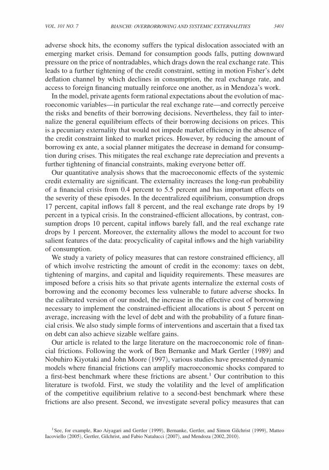
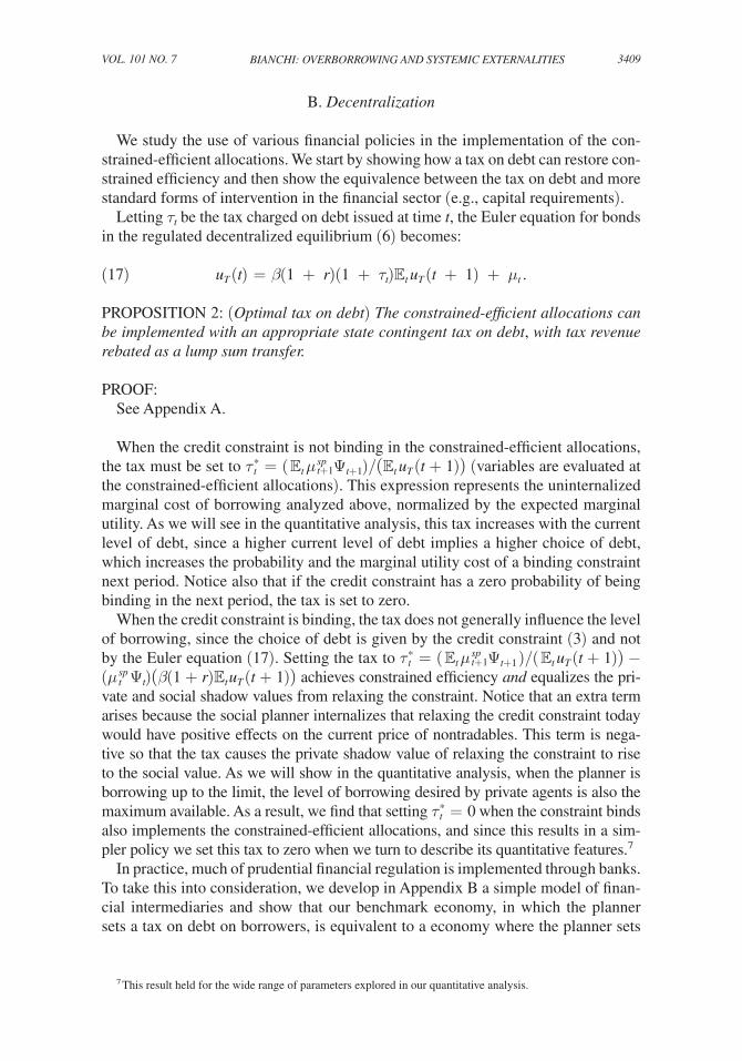
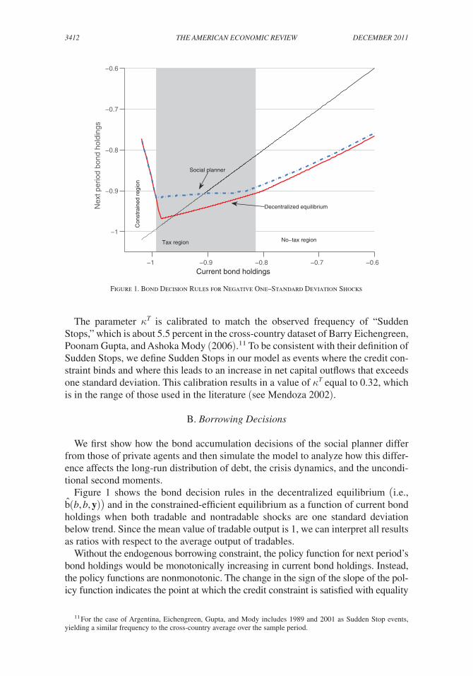
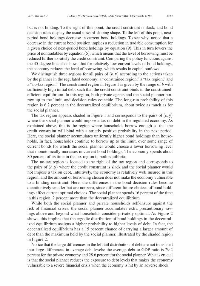
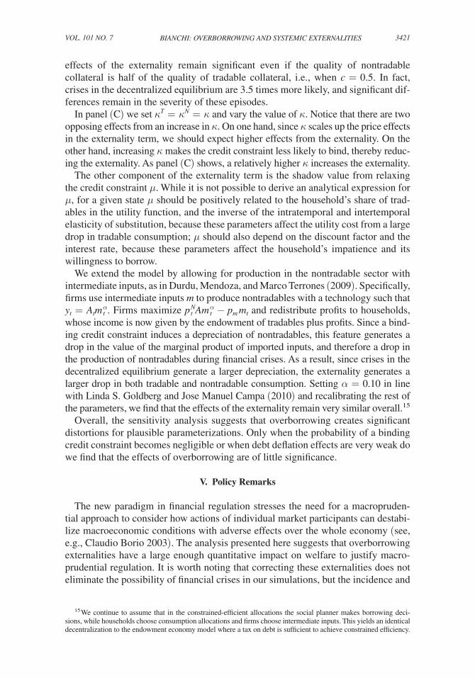
Figure 1 shows the bond decision rules in the decentralized equilibrium (i.e., b (b, b, y)) and in the constrained-efficient equilibrium as a function of current bond holdings when both tradable and nontradable shocks are one standard deviation below trend. Since the mean value of tradable output is 1, we can interpret all results as ratios with respect to the average output of tradables.
Without the endogenous borrowing constraint, the policy function for next period’s bond holdings would be monotonically increasing in current bond holdings. Instead, the policy functions are nonmonotonic. The change in the sign of the slope of the pol-icy function indicates the point at which the credit constraint is satisfied with equality
11 For the case of Argentina, Eichengreen, Gupta, and Mody includes 1989 and 2001 as Sudden Stop events, yielding a similar frequency to the cross-country average over the sample period.
Figure 1. Bond Decision Rules for Negative One–Standard Deviation Shocks
−1 −0.9 −0.8 −0.7 −0.6
−1
−0.9
−0.8
−0.7
−0.6
Current bond holdings
Nex
t per
iod
bond
hol
ding
s
Tax region No−tax region
Con
stra
ined
reg
ion
Social planner
Decentralized equilibrium
3413BiAnchi: OvERBORROwing AnD SyStEmic ExtERnAlitiESvOl. 101 nO. 7
but is not binding. To the right of this point, the credit constraint is slack, and bond decision rules display the usual upward-sloping shape. To the left of this point, next-period bond holdings decrease in current bond holdings. To see why, notice that a decrease in the current bond position implies a reduction in tradable consumption for a given choice of next-period bond holdings by equation (9). This in turn lowers the price of nontradables by equation (5), which means that the level of borrowing must be reduced further to satisfy the credit constraint. Comparing the policy functions against the 45-degree line also shows that for relatively low current levels of bond holdings, the economy reduces the level of borrowing, which results in capital outflows.
We distinguish three regions for all pairs of (b, y) according to the actions taken by the planner in the regulated economy: a “constrained region,” a “tax region,” and a “no-tax region.” The constrained region in Figure 1 is given by the range of b with sufficiently high initial debt such that the credit constraint binds in the constrained-efficient equilibrium. In this region, both private agents and the social planner bor-row up to the limit, and decision rules coincide. The long-run probability of this region is 6.2 percent in the decentralized equilibrium, about twice as much as for the social planner.
The tax region appears shaded in Figure 1 and corresponds to the pairs of (b, y) where the social planner would impose a tax on debt in the regulated economy. As explained above, this is the region where households borrow enough so that the credit constraint will bind with a strictly positive probability in the next period. Here, the social planner accumulates uniformly higher bond holdings than house-holds. In fact, households continue to borrow up to the limit, over some range of current bonds for which the social planner would choose a lower borrowing level that monotonically increases in current bond holdings. The economy spends about 80 percent of its time in the tax region in both equilibria.
The no-tax region is located to the right of the tax region and corresponds to the pairs of (b, y) where the credit constraint is slack and the social planner would not impose a tax on debt. Intuitively, the economy is relatively well insured in this region, and the amount of borrowing chosen does not make the economy vulnerable to a binding constraint. Here, the differences in the bond decision rules become quantitatively smaller but are nonzero, since different future choices of bond hold-ings affect current optimal choices. The social planner spends 16 percent of the time in this region, 2 percent more than the decentralized equilibrium.
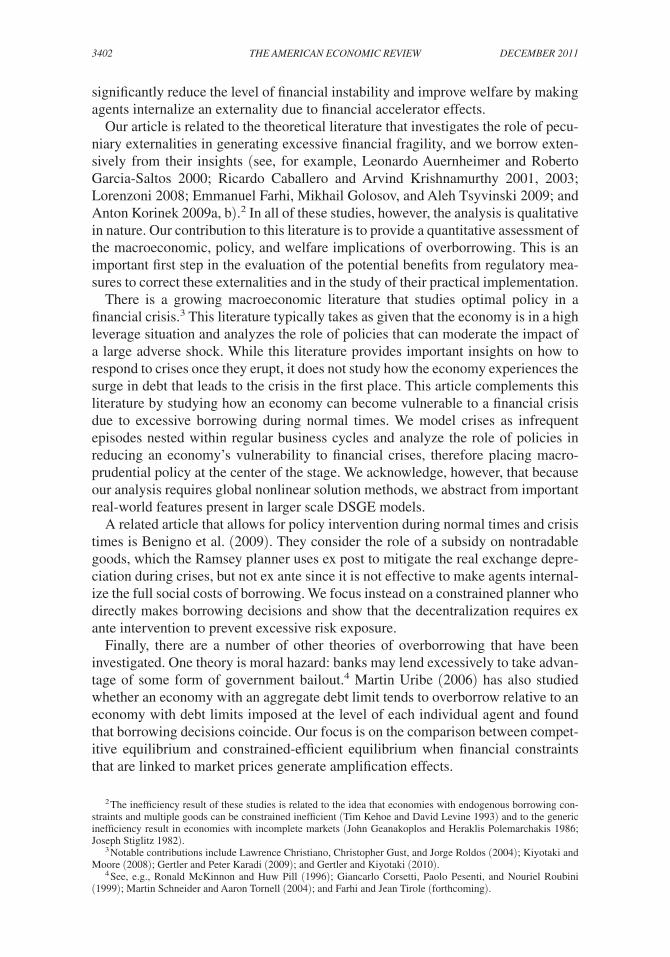
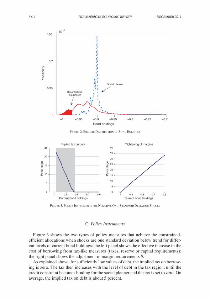
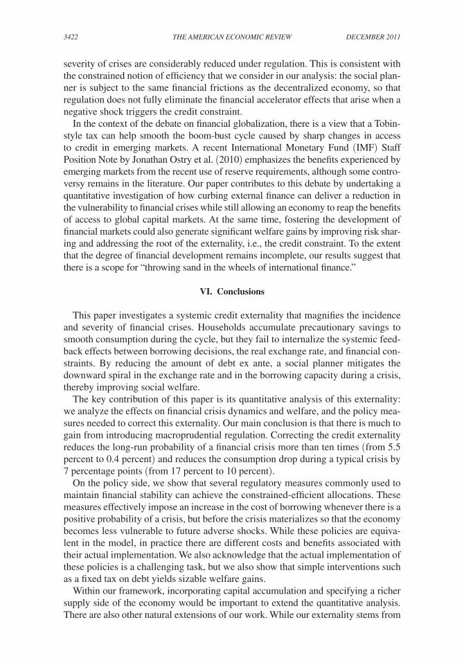
While both the social planner and private households self-insure against the risk of financial crises, the social planner accumulates extra precautionary sav-ings above and beyond what households consider privately optimal. As Figure 2 shows, this implies that the ergodic distribution of bond holdings in the decentral-ized equilibrium assigns a higher probability to higher levels of debt. In fact, the decentralized equilibrium has a 15 percent chance of carrying a larger amount of debt than the maximum held by the social planner, illustrated by the shaded region in Figure 2.
Notice that the large differences in the left tail distribution of debt are not translated into large differences in average debt levels: the average debt-to-GDP ratio is 29.2 percent for the private economy and 28.6 percent for the social planner. What is crucial is that the social planner reduces the exposure to debt levels that makes the economy vulnerable to a severe financial crisis when the economy is hit by an adverse shock.
3414 thE AmERicAn EcOnOmic REviEw DEcEmBER 2011
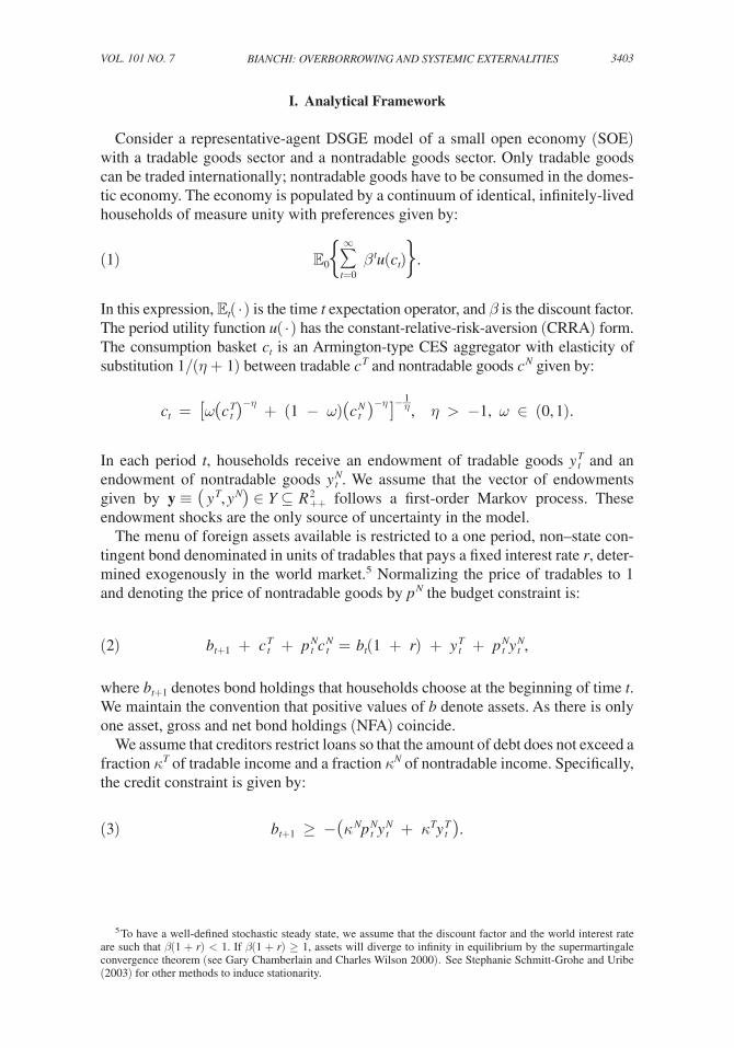
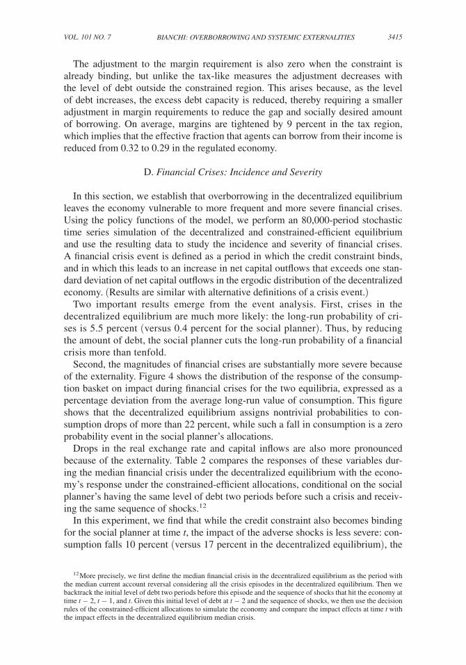
C. Policy instruments
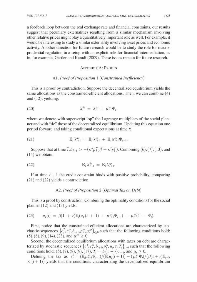
Figure 3 shows the two types of policy measures that achieve the constrained-efficient allocations when shocks are one standard deviation below trend for differ-ent levels of current bond holdings: the left panel shows the effective increase in the cost of borrowing from tax-like measures (taxes, reserve or capital requirements); the right panel shows the adjustment in margin requirements θ.
As explained above, for sufficiently low values of debt, the implied tax on borrow-ing is zero. The tax then increases with the level of debt in the tax region, until the credit constraint becomes binding for the social planner and the tax is set to zero. On average, the implied tax on debt is about 5 percent.
Figure 2. Ergodic Distribution of Bond Holdings
−1 −0.95 −0.9 −0.85 −0.8 −0.75 −0.70
0.35
0.7
1.05x 10⁻³
Bond holdings
Pro
babi
lity
Social planner
Decentralized equilibrium
Figure 3. Policy Instruments for Negative One–Standard Deviation Shocks
−1 −0.9 −0.8 −0.7 −0.60
5
10
15
20
25
Current bond holdings
Per
cent
age
Implied tax on debt
−1 −0.9 −0.8 −0.7 −0.60
5
10
15
20
25
30
35
40Tightening of margins
Current bond holdings
Per
cent
age
3415BiAnchi: OvERBORROwing AnD SyStEmic ExtERnAlitiESvOl. 101 nO. 7
The adjustment to the margin requirement is also zero when the constraint is already binding, but unlike the tax-like measures the adjustment decreases with the level of debt outside the constrained region. This arises because, as the level of debt increases, the excess debt capacity is reduced, thereby requiring a smaller adjustment in margin requirements to reduce the gap and socially desired amount of borrowing. On average, margins are tightened by 9 percent in the tax region, which implies that the effective fraction that agents can borrow from their income is reduced from 0.32 to 0.29 in the regulated economy.
D. Financial crises: incidence and Severity
In this section, we establish that overborrowing in the decentralized equilibrium leaves the economy vulnerable to more frequent and more severe financial crises. Using the policy functions of the model, we perform an 80,000-period stochastic time series simulation of the decentralized and constrained-efficient equilibrium and use the resulting data to study the incidence and severity of financial crises. A financial crisis event is defined as a period in which the credit constraint binds, and in which this leads to an increase in net capital outflows that exceeds one stan-dard deviation of net capital outflows in the ergodic distribution of the decentralized economy. (Results are similar with alternative definitions of a crisis event.)
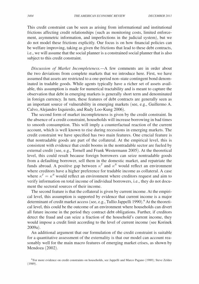
Two important results emerge from the event analysis. First, crises in the decentralized equilibrium are much more likely: the long-run probability of cri-ses is 5.5 percent (versus 0.4 percent for the social planner). Thus, by reducing the amount of debt, the social planner cuts the long-run probability of a financial crisis more than tenfold.
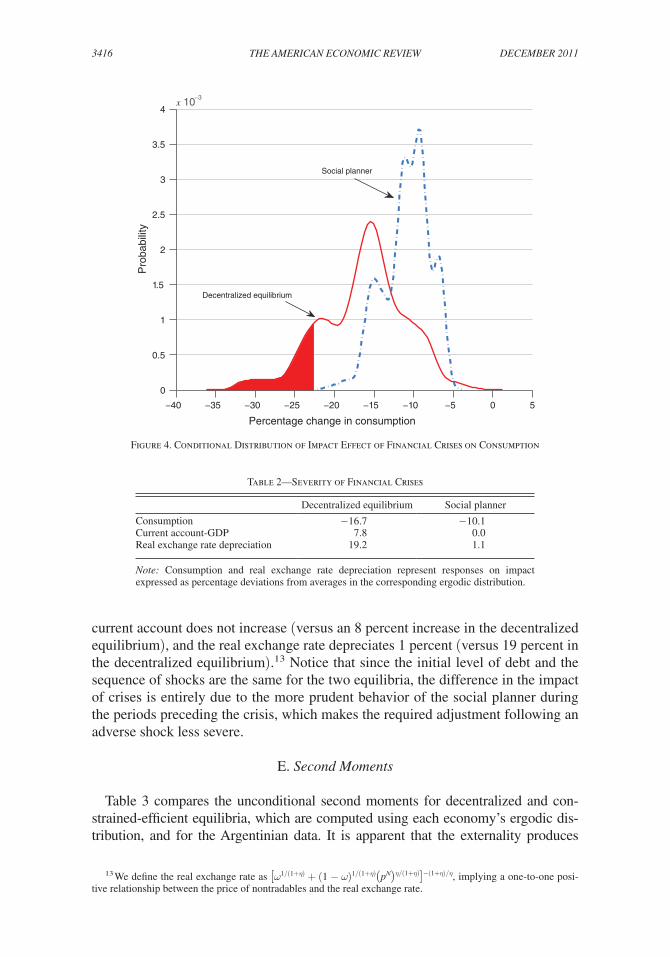
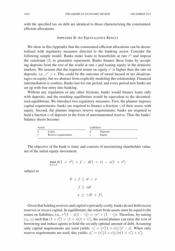
Second, the magnitudes of financial crises are substantially more severe because of the externality. Figure 4 shows the distribution of the response of the consump-tion basket on impact during financial crises for the two equilibria, expressed as a percentage deviation from the average long-run value of consumption. This figure shows that the decentralized equilibrium assigns nontrivial probabilities to con-sumption drops of more than 22 percent, while such a fall in consumption is a zero probability event in the social planner’s allocations.
Drops in the real exchange rate and capital inflows are also more pronounced because of the externality. Table 2 compares the responses of these variables dur-ing the median financial crisis under the decentralized equilibrium with the econo-my’s response under the constrained-efficient allocations, conditional on the social planner’s having the same level of debt two periods before such a crisis and receiv-ing the same sequence of shocks.12
In this experiment, we find that while the credit constraint also becomes binding for the social planner at time t, the impact of the adverse shocks is less severe: con-sumption falls 10 percent (versus 17 percent in the decentralized equilibrium), the
12 More precisely, we first define the median financial crisis in the decentralized equilibrium as the period with the median current account reversal considering all the crisis episodes in the decentralized equilibrium. Then we backtrack the initial level of debt two periods before this episode and the sequence of shocks that hit the economy at time t − 2, t − 1, and t. Given this initial level of debt at t − 2 and the sequence of shocks, we then use the decision rules of the constrained-efficient allocations to simulate the economy and compare the impact effects at time t with the impact effects in the decentralized equilibrium median crisis.
3416 thE AmERicAn EcOnOmic REviEw DEcEmBER 2011
current account does not increase (versus an 8 percent increase in the decentralized equilibrium), and the real exchange rate depreciates 1 percent (versus 19 percent in the decentralized equilibrium).13 Notice that since the initial level of debt and the sequence of shocks are the same for the two equilibria, the difference in the impact of crises is entirely due to the more prudent behavior of the social planner during the periods preceding the crisis, which makes the required adjustment following an adverse shock less severe.
E. Second moments
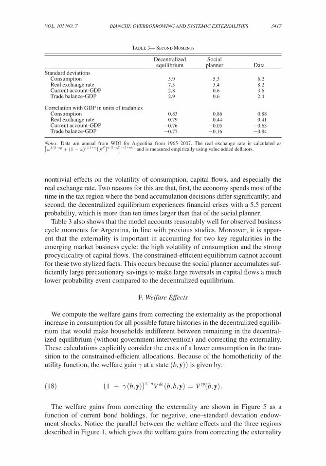
Table 3 compares the unconditional second moments for decentralized and con-strained-efficient equilibria, which are computed using each economy’s ergodic dis-tribution, and for the Argentinian data. It is apparent that the externality produces
13 We define the real exchange rate as [ ω 1/(1+η) + (1 − ω ) 1/(1+η) ( p n ) η/(1+η) ] −(1+η)/η , implying a one-to-one posi-tive relationship between the price of nontradables and the real exchange rate.
Figure 4. Conditional Distribution of Impact Effect of Financial Crises on Consumption
−40 −35 −30 −25 −20 −15 −10 −5 0 5
0
0.5
1
1.5
2
2.5
3
3.5
4x 10⁻³
Percentage change in consumption
Pro
babi
lity
Social planner
Decentralized equilibrium
Table 2—Severity of Financial Crises
Decentralized equilibrium Social planner
Consumption −16.7 −10.1Current account-GDP 7.8 0.0Real exchange rate depreciation 19.2 1.1
note: Consumption and real exchange rate depreciation represent responses on impact expressed as percentage deviations from averages in the corresponding ergodic distribution.
3417BiAnchi: OvERBORROwing AnD SyStEmic ExtERnAlitiESvOl. 101 nO. 7
nontrivial effects on the volatility of consumption, capital flows, and especially the real exchange rate. Two reasons for this are that, first, the economy spends most of the time in the tax region where the bond accumulation decisions differ significantly; and second, the decentralized equilibrium experiences financial crises with a 5.5 percent probability, which is more than ten times larger than that of the social planner.
Table 3 also shows that the model accounts reasonably well for observed business cycle moments for Argentina, in line with previous studies. Moreover, it is appar-ent that the externality is important in accounting for two key regularities in the emerging market business cycle: the high volatility of consumption and the strong procyclicality of capital flows. The constrained-efficient equilibrium cannot account for these two stylized facts. This occurs because the social planner accumulates suf-ficiently large precautionary savings to make large reversals in capital flows a much lower probability event compared to the decentralized equilibrium.
F. welfare Effects
We compute the welfare gains from correcting the externality as the proportional increase in consumption for all possible future histories in the decentralized equilib-rium that would make households indifferent between remaining in the decentral-ized equilibrium (without government intervention) and correcting the externality. These calculations explicitly consider the costs of a lower consumption in the tran-sition to the constrained-efficient allocations. Because of the homotheticity of the utility function, the welfare gain γ at a state (b, y)) is given by:
(18) (1 + γ (b, y) ) 1−σ v de (b, b, y) = v sp (b, y) .
The welfare gains from correcting the externality are shown in Figure 5 as a function of current bond holdings, for negative, one–standard deviation endow-ment shocks. Notice the parallel between the welfare effects and the three regions described in Figure 1, which gives the welfare gains from correcting the externality
Table 3— Second Moments
Decentralized Socialequilibrium planner Data
Standard deviations Consumption 5.9 5.3 6.2 Real exchange rate 7.5 3.4 8.2 Current account-GDP 2.8 0.6 3.6 Trade balance-GDP 2.9 0.6 2.4
Correlation with GDP in units of tradables Consumption 0.83 0.86 0.88 Real exchange rate 0.79 0.44 0.41 Current account-GDP −0.76 −0.05 −0.63 Trade balance-GDP −0.77 −0.16 −0.84
notes: Data are annual from WDI for Argentina from 1965–2007. The real exchange rate is calculated as [ ω 1/(1+η) + (1 − ω ) 1/(1+η) ( p n ) η/(1+η) ] −(1+η)/η and is measured empirically using value added deflators.
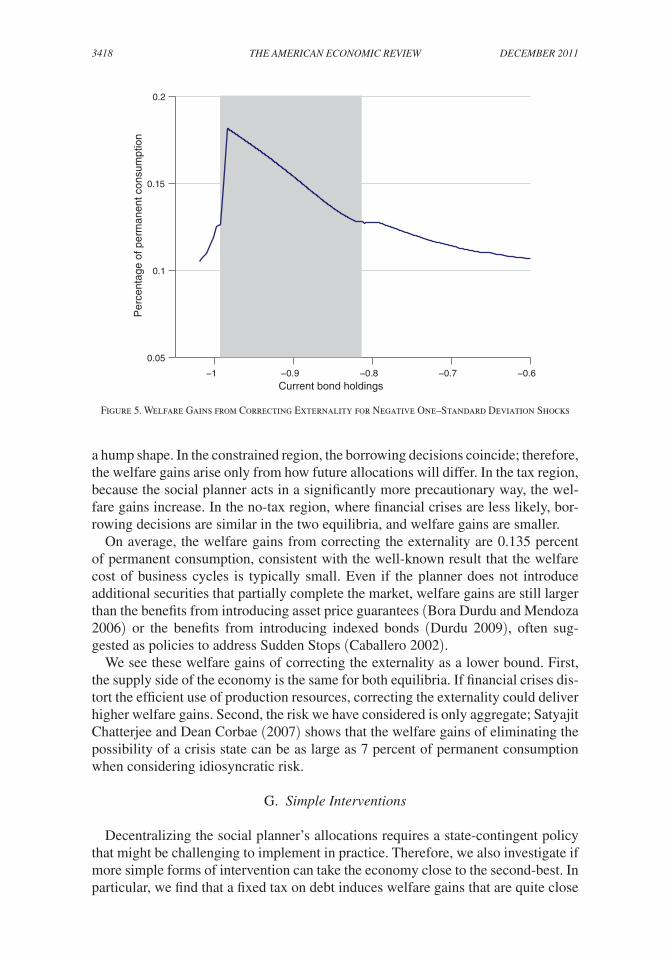
3418 thE AmERicAn EcOnOmic REviEw DEcEmBER 2011
a hump shape. In the constrained region, the borrowing decisions coincide; therefore, the welfare gains arise only from how future allocations will differ. In the tax region, because the social planner acts in a significantly more precautionary way, the wel-fare gains increase. In the no-tax region, where financial crises are less likely, bor-rowing decisions are similar in the two equilibria, and welfare gains are smaller.
On average, the welfare gains from correcting the externality are 0.135 percent of permanent consumption, consistent with the well-known result that the welfare cost of business cycles is typically small. Even if the planner does not introduce additional securities that partially complete the market, welfare gains are still larger than the benefits from introducing asset price guarantees (Bora Durdu and Mendoza 2006) or the benefits from introducing indexed bonds (Durdu 2009), often sug-gested as policies to address Sudden Stops (Caballero 2002).
We see these welfare gains of correcting the externality as a lower bound. First, the supply side of the economy is the same for both equilibria. If financial crises dis-tort the efficient use of production resources, correcting the externality could deliver higher welfare gains. Second, the risk we have considered is only aggregate; Satyajit Chatterjee and Dean Corbae (2007) shows that the welfare gains of eliminating the possibility of a crisis state can be as large as 7 percent of permanent consumption when considering idiosyncratic risk.
G. Simple interventions
Decentralizing the social planner’s allocations requires a state-contingent policy that might be challenging to implement in practice. Therefore, we also investigate if more simple forms of intervention can take the economy close to the second-best. In particular, we find that a fixed tax on debt induces welfare gains that are quite close
Figure 5. Welfare Gains from Correcting Externality for Negative One–Standard Deviation Shocks
−1 −0.9 −0.8 −0.7 −0.6
0.05
0.1
0.15
0.2
Current bond holdings
Per
cent
age
of p
erm
anen
t con
sum
ptio
n
3419BiAnchi: OvERBORROwing AnD SyStEmic ExtERnAlitiESvOl. 101 nO. 7
to the second-best solution. The optimal fixed tax is 3.6 percent, which is about 70 percent of the average of the state-contingent tax and achieves 62 percent of the welfare gains from implementing the constrained-efficient allocations. This fixed tax cuts by more than half the probability of a crisis. Allowing the tax to drop to zero when the credit constraint binds in the regulated economy, or in the constrained region, delivers about the same welfare gains as the fixed tax.
By contrast, a fixed tightening in margins across all states of nature delivers wel-fare losses. This is intuitive given that tightening margins when the constraint is already binding delivers significant welfare losses, which outweigh the benefits from a lower average amount of debt. Tightening margins outside the constrained-efficient equilibrium only, however, can generate welfare gains, albeit smaller gains than a fixed tax on borrowing.
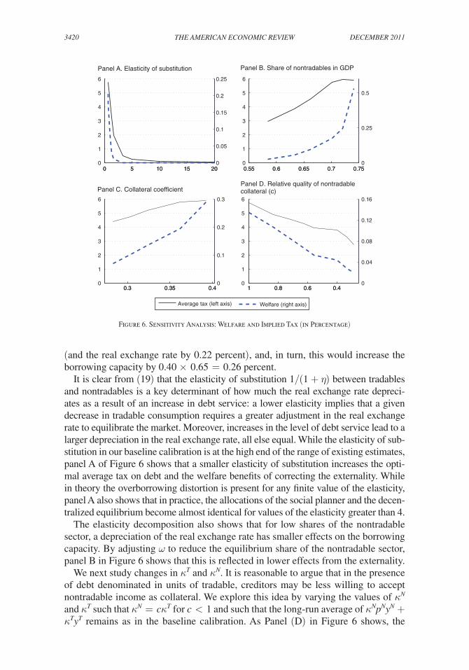
H. Sensitivity Analysis
In this section, we examine the sensitivity of our results to alternative calibrations. Figure 6 shows how the average welfare effects and the optimal average tax on debt vary with some key parameters. The online Appendix includes results from chang-ing all parameter values and details of the sensitivity analysis.
We can gain a better understanding of the results by analyzing the externality term μ t
sp Ψ t , which is the wedge between the social shadow value of wealth and the private shadow value of wealth. Recalling that Ψ t ≡ κ n ( p t
n c t n )/( c t
t )(1 + η), we have that the fraction of nontradable output that can be collateralized, the size of the nontrad-able sector, and the elasticity of substitution are the key parameters determining the price effects in the externality term.
To arrive to a unit free measure of how the different parameters affect the price responses, we decompose the effects of the different parameters in terms of elastici-ties. Two elasticities are crucial for determining the price effects on the borrowing capacity. First is the elasticity that measures how much the depreciation of nontrad-ables tightens the borrowing constraint. Second is the elasticity that measures how much nontradables depreciate as a result of an increase in debt service. Denoting the borrowing limit by Δ ≡ κ n p n y n + κ t y t , debt service by DS ≡ b(1 + r) − b′, and the elasticity of y with respect to x by ε y, x , we can decompose the elasticity of the borrowing limit with respect to debt service as the product of these two elasticities:14
(19) ε Δ, DS = ( p n y n _ y t + p n y n
) ((η + 1) DS _ y t − DS
). 3 8 ε Δ, p n ε p n , DS
In the baseline calibration, ε Δ, p n = 0.65 and ε p n , DS = 0.40 at the median crisis in the decentralized equilibrium. That is, a reduction in the debt service of 1 percent would mitigate the drop in the price of nontradables during a median crisis by 0.40 percent
14 This formula yields as a result of applying the definition of Δ and DS, the three elasticities, and using Ψ = − (∂Δ)/(∂DS ).
3420 thE AmERicAn EcOnOmic REviEw DEcEmBER 2011
(and the real exchange rate by 0.22 percent), and, in turn, this would increase the borrowing capacity by 0.40 × 0.65 = 0.26 percent.
It is clear from (19) that the elasticity of substitution 1/(1 + η) between tradables and nontradables is a key determinant of how much the real exchange rate depreci-ates as a result of an increase in debt service: a lower elasticity implies that a given decrease in tradable consumption requires a greater adjustment in the real exchange rate to equilibrate the market. Moreover, increases in the level of debt service lead to a larger depreciation in the real exchange rate, all else equal. While the elasticity of sub-stitution in our baseline calibration is at the high end of the range of existing estimates, panel A of Figure 6 shows that a smaller elasticity of substitution increases the opti-mal average tax on debt and the welfare benefits of correcting the externality. While in theory the overborrowing distortion is present for any finite value of the elasticity, panel A also shows that in practice, the allocations of the social planner and the decen-tralized equilibrium become almost identical for values of the elasticity greater than 4.
The elasticity decomposition also shows that for low shares of the nontradable sector, a depreciation of the real exchange rate has smaller effects on the borrowing capacity. By adjusting ω to reduce the equilibrium share of the nontradable sector, panel B in Figure 6 shows that this is reflected in lower effects from the externality.
We next study changes in κ t and κ n . It is reasonable to argue that in the presence of debt denominated in units of tradable, creditors may be less willing to accept nontradable income as collateral. We explore this idea by varying the values of κ n and κ t such that κ n = c κ t for c < 1 and such that the long-run average of κ n p n y n + κ t y t remains as in the baseline calibration. As Panel (D) in Figure 6 shows, the
Figure 6. Sensitivity Analysis: Welfare and Implied Tax (in Percentage)
0 5 10 15 200
1
2
3
4
5
6
0 5 10 15 200
0.05
0.1
0.15
0.2
0.25
Panel A. Elasticity of substitution
0.55 0.6 0.65 0.7 0.750
1
2
3
4
5
6
0.55 0.6 0.65 0.7 0.750
0.25
0.5
Panel B. Share of nontradables in GDP
0.3 0.35 0.40
1
2
3
4
5
6
0.3 0.35 0.40
0.1
0.2
0.3
Panel C. Collateral coefficient
0.40.60.810
1
2
3
4
5
6
0.40.60.810
0.04
0.08
0.12
0.16
Panel D. Relative quality of nontradable collateral (c)
Average tax (left axis) Welfare (right axis)
3421BiAnchi: OvERBORROwing AnD SyStEmic ExtERnAlitiESvOl. 101 nO. 7
effects of the externality remain significant even if the quality of nontradable collateral is half of the quality of tradable collateral, i.e., when c = 0.5. In fact, crises in the decentralized equilibrium are 3.5 times more likely, and significant dif-ferences remain in the severity of these episodes.
In panel (C) we set κ t = κ n = κ and vary the value of κ. Notice that there are two opposing effects from an increase in κ. On one hand, since κ scales up the price effects in the externality term, we should expect higher effects from the externality. On the other hand, increasing κ makes the credit constraint less likely to bind, thereby reduc-ing the externality. As panel (C) shows, a relatively higher κ increases the externality.
The other component of the externality term is the shadow value from relaxing the credit constraint μ. While it is not possible to derive an analytical expression for μ, for a given state μ should be positively related to the household’s share of trad-ables in the utility function, and the inverse of the intratemporal and intertemporal elasticity of substitution, because these parameters affect the utility cost from a large drop in tradable consumption; μ should also depend on the discount factor and the interest rate, because these parameters affect the household’s impatience and its willingness to borrow.
We extend the model by allowing for production in the nontradable sector with intermediate inputs, as in Durdu, Mendoza, and Marco Terrones (2009). Specifically, firms use intermediate inputs m to produce nontradables with a technology such that y t = A t m t
α . Firms maximize p t n A m t
α − p m m t and redistribute profits to households, whose income is now given by the endowment of tradables plus profits. Since a bind-ing credit constraint induces a depreciation of nontradables, this feature generates a drop in the value of the marginal product of imported inputs, and therefore a drop in the production of nontradables during financial crises. As a result, since crises in the decentralized equilibrium generate a larger depreciation, the externality generates a larger drop in both tradable and nontradable consumption. Setting α = 0.10 in line with Linda S. Goldberg and Jose Manuel Campa (2010) and recalibrating the rest of the parameters, we find that the effects of the externality remain very similar overall.15
Overall, the sensitivity analysis suggests that overborrowing creates significant distortions for plausible parameterizations. Only when the probability of a binding credit constraint becomes negligible or when debt deflation effects are very weak do we find that the effects of overborrowing are of little significance.
V. Policy Remarks
The new paradigm in financial regulation stresses the need for a macropruden-tial approach to consider how actions of individual market participants can destabi-lize macroeconomic conditions with adverse effects over the whole economy (see, e.g., Claudio Borio 2003). The analysis presented here suggests that overborrowing externalities have a large enough quantitative impact on welfare to justify macro-prudential regulation. It is worth noting that correcting these externalities does not eliminate the possibility of financial crises in our simulations, but the incidence and
15 We continue to assume that in the constrained-efficient allocations the social planner makes borrowing deci-sions, while households choose consumption allocations and firms choose intermediate inputs. This yields an identical decentralization to the endowment economy model where a tax on debt is sufficient to achieve constrained efficiency.
3422 thE AmERicAn EcOnOmic REviEw DEcEmBER 2011
severity of crises are considerably reduced under regulation. This is consistent with the constrained notion of efficiency that we consider in our analysis: the social plan-ner is subject to the same financial frictions as the decentralized economy, so that regulation does not fully eliminate the financial accelerator effects that arise when a negative shock triggers the credit constraint.
In the context of the debate on financial globalization, there is a view that a Tobin-style tax can help smooth the boom-bust cycle caused by sharp changes in access to credit in emerging markets. A recent International Monetary Fund (IMF) Staff Position Note by Jonathan Ostry et al. (2010) emphasizes the benefits experienced by emerging markets from the recent use of reserve requirements, although some contro-versy remains in the literature. Our paper contributes to this debate by undertaking a quantitative investigation of how curbing external finance can deliver a reduction in the vulnerability to financial crises while still allowing an economy to reap the benefits of access to global capital markets. At the same time, fostering the development of financial markets could also generate significant welfare gains by improving risk shar-ing and addressing the root of the externality, i.e., the credit constraint. To the extent that the degree of financial development remains incomplete, our results suggest that there is a scope for “throwing sand in the wheels of international finance.”
VI. Conclusions
This paper investigates a systemic credit externality that magnifies the incidence and severity of financial crises. Households accumulate precautionary savings to smooth consumption during the cycle, but they fail to internalize the systemic feed-back effects between borrowing decisions, the real exchange rate, and financial con-straints. By reducing the amount of debt ex ante, a social planner mitigates the downward spiral in the exchange rate and in the borrowing capacity during a crisis, thereby improving social welfare.
The key contribution of this paper is its quantitative analysis of this externality: we analyze the effects on financial crisis dynamics and welfare, and the policy mea-sures needed to correct this externality. Our main conclusion is that there is much to gain from introducing macroprudential regulation. Correcting the credit externality reduces the long-run probability of a financial crisis more than ten times (from 5.5 percent to 0.4 percent) and reduces the consumption drop during a typical crisis by 7 percentage points (from 17 percent to 10 percent).
On the policy side, we show that several regulatory measures commonly used to maintain financial stability can achieve the constrained-efficient allocations. These measures effectively impose an increase in the cost of borrowing whenever there is a positive probability of a crisis, but before the crisis materializes so that the economy becomes less vulnerable to future adverse shocks. While these policies are equiva-lent in the model, in practice there are different costs and benefits associated with their actual implementation. We also acknowledge that the actual implementation of these policies is a challenging task, but we also show that simple interventions such as a fixed tax on debt yields sizable welfare gains.
Within our framework, incorporating capital accumulation and specifying a richer supply side of the economy would be important to extend the quantitative analysis. There are also other natural extensions of our work. While our externality stems from
3423BiAnchi: OvERBORROwing AnD SyStEmic ExtERnAlitiESvOl. 101 nO. 7
a feedback loop between the real exchange rate and financial constraints, our results suggest that pecuniary externalities resulting from a similar mechanism involving other relative prices might play a quantitatively important role as well. For example, it would be interesting to study a similar externality involving asset prices and economic activity. Another direction for future research would be to study the role for macro-prudential regulation in a setup with an explicit role for financial intermediation, as in, for example, Gertler and Karadi (2009). These issues remain for future research.
Appendix A: Proofs
A1. Proof of Proposition 1 (constrained inefficiency)
This is a proof by contradiction. Suppose the decentralized equilibrium yields the same allocations as the constrained-efficient allocations. Then, we can combine (4) and (12), yielding:
(20) λ t de = λ t
sp + μ t sp Ψ t ,
where we denote with superscript “sp” the Lagrange multipliers of the social plan-ner and with “de” those of the decentralized equilibrium. Updating this equation one period forward and taking conditional expectations at time t:
(21) 피 t λ t+1 de
= 피 t λ t+1 sp
+ 피 t μ t+1 sp
Ψ t+1 .
Suppose that at time ̃ t , b ̃ t +1 > − ( κ n p ̃ t n y ̃ t
n + κ t y ̃ t t ). Combining (6), (7), (13), and
(14) we obtain:
(22) 피 ̃ t λ ̃ t +1 de
= 피 ̃ t λ ̃ t +1 sp
.
If at time ̃ t + 1 the credit constraint binds with positive probability, comparing (21) and (22) yields a contradiction.
A2. Proof of Proposition 2 (Optimal tax on Debt)
This is a proof by construction. Combining the optimality conditions for the social planner (12) and (13) yields:
(23) u t (t) = β(1 + r) 피 t ( u t (t + 1) + μ t+1 sp
Ψ t+1 ) + μ t sp (1 − Ψ t ).
First, notice that the constrained-efficient allocations are characterized by sto-chastic sequences {c t
t , c t n , b t+1 , p t
n , μ t sp } t≥0 such that the following conditions hold:
(5), (8), (9), (14), (23), and μ t sp ≥ 0.
Second, the decentralized equilibrium allocations with taxes on debt are charac-terized by stochastic sequences { c t
t , c t n , b t+1 , p t
n , μ t , τ t , t t } t≥0 such that the following conditions hold: (5), (7), (8), (9), (17), t t = b t (1 + r) τ t−1 , and μ t ≥ 0.
Defining the tax as τ t * = ( 피 t μ t+1 sp
Ψ t+1 )/( 피 t u t (t + 1)) − ( μ t sp Ψ t )/(β(1 + r) 피 t u t
× (t + 1)) yields that the conditions characterizing the decentralized equilibrium
3424 thE AmERicAn EcOnOmic REviEw DEcEmBER 2011
with the specified tax on debt are identical to those characterizing the constrained-efficient allocations.
Appendix B: An Equivalence Result
We show in this Appendix that the constrained-efficient allocations can be decen-tralized with regulatory measures directed to the banking sector. Consider the following simple model. Banks make loans to households at rate r l and impose the constraint (2) to guarantee repayment. Banks finance these loans by accept-ing deposits from the rest of the world at rate r and issuing equity in the domestic markets. We assume that the required return on equity r e is higher than the rate on deposits, i.e., r e > r. This could be the outcome of moral hazard or tax disadvan-tages on equity, but we abstract from explicitly modeling this relationship. Financial intermediation is costless. Banks last for one period, and every period new banks are set up with free entry into banking.
Without any regulation or any other frictions, banks would finance loans only with deposits, and the resulting equilibrium would be equivalent to the decentral-ized equilibrium. We introduce two regulatory measures. First, the planner imposes capital requirements: banks are required to finance a fraction γ of their assets with equity. Second, the planner imposes reserve requirements: banks are required to hold a fraction ϕ of deposits in the form of unremunerated reserve. Thus the banks’ balance sheets become:
Assets Liabilities
b Loans d Depositsf Reserve requirements e Equity
The objective of the bank is static and consists of maximizing shareholder value, net of the initial equity investment:
max b, f, e, d
b(1 + r l ) + f − d(1 + r) − e(1 + r e )
subject to
b + f ≤ d + e
f ≥ ϕd
e ≥ γ (b + f ).
Given that holding reserves and capital is privately costly, banks do not hold excess reserves or excess capital. In equilibrium, the return from assets must be equal to the return on liabilities, i.e., r l (1 − ϕ(1 − γ)) = γ r e + (1 − γ)r. Therefore, by setting ( ϕ t , γ t ) such that (1 + r t
l ) = (1 + r)(1 + τ t * ), the social planner can raise the cost of borrowing and induce agents to hold the socially optimal amount of debt. Assuming only capital requirements are used yields: γ t * = ( τ t * (1 + r))/( r e − r). When only reserve requirements are used, this yields: ϕ t * = ( τ t * (1 + r))/(r(1 + τ t * ) + τ t * ).
3425BiAnchi: OvERBORROwing AnD SyStEmic ExtERnAlitiESvOl. 101 nO. 7
REFERENCES
Aiyagari, S. Rao, and Mark Gertler. 1999. “’Overreaction’ Of Asset Prices in General Equilibrium.” Review of Economic Dynamics, 2(1): 3–35.
Auernheimer, Leonardo, and Roberto Garcia-Saltos. 2000. “International Debt and the Price of Domestic Assets.” International Monetary Fund Working Paper 00/177.
Benigno, Gianluca, Huigang Chen, Christopher Otrok, Alessandro Rebucci, and Eric R. Young. 2009. “Optimal Stabilization Policy in a Model with Endogenous Sudden Stops.” Unpublished.
Bernanke, Ben, and Mark Gertler. 1989. “Agency Costs, Net Worth, and Business Fluctuations.” American Economic Review, 79(1): 14–31.
Bernanke, Ben S., Mark Gertler, and Simon Gilchrist. 1999. “The Financial Accelerator in a Quantita-tive Business Cycle Framework.” In handbook of macroeconomics, volume 1c. Vol. 15, Handbooks in Economics, ed. J. B. Taylor and M. Woodford, 1341–93. New York: Elsevier Science.
Bianchi, Javier. 2011. “Overborrowing and Systemic Externalities in the Business Cycle: Dataset.” American Economic Review. http://www.aeaweb.org/articles.php?doi=10.1257/aer.101.7.3400.
Borio, Claudio. 2003. “Towards a Macroprudential Framework for Financial Supervision and Regula-tion?” cESifo Economic Studies, 49(2): 181–215.
Caballero, Ricardo J. 2002. “Coping with Chile’s External Vulnerability: A Financial Problem.” In Economic growth: Sources, trends, and cycles. Vol. 6, Series on Central Banking, Analysis, and Economic Policies, ed. N. Loayza and R. Soto, 377–415. Santiago: Central Bank of Chile.
Caballero, Ricardo J., and Arvind Krishnamurthy. 2001. “International and Domestic Collateral Con-straints in a Model of Emerging Market Crises.” Journal of monetary Economics, 48(3): 513–48.
Caballero, Ricardo J., and Arvind Krishnamurthy. 2003. “Excessive Dollar Debt: Financial Develop-ment and Underinsurance.” Journal of Finance, 58(2): 867–93.
Calvo, Guillermo A., Alejandro Izquierdo, and Rudy Loo-Kung. 2006. “Relative Price Volatility under Sudden Stops: The Relevance of Balance Sheet Effects.” Journal of international Economics, 69(1): 231–54.
Chamberlain, Gary, and Charles A. Wilson. 2000. “Optimal Intertemporal Consumption under Uncer-tainty.” Review of Economic Dynamics, 3(3): 365–95.
Chatterjee, Satyajit, and Dean Corbae. 2007. “On the Aggregate Welfare Cost of Great Depression Unemployment.” Journal of monetary Economics, 54(6): 1529–44.
Christiano, Lawrence J., Christopher Gust, and Jorge Roldos. 2004. “Monetary Policy in a Financial Crisis.” Journal of Economic theory, 119(1): 64–103.
Corsetti, Giancarlo, Paolo Pesenti, and Nouriel Roubini. 1999. “Paper Tigers? A Model of the Asian Crisis.” European Economic Review, 43(7): 1211–36.
Durdu, Ceyhun Bora. 2009. “Quantitative Implications of Indexed Bonds in Small Open Economies.” Journal of Economic Dynamics and control, 33(4): 883–902.
Durdu, Ceyhun Bora, and Enrique G. Mendoza. 2006. “Are Asset Price Guarantees Useful for Pre-venting Sudden Stops?: A Quantitative Investigation of the Globalization Hazard-Moral Hazard Tradeoff.” Journal of international Economics, 69(1): 84–119.
Durdu, Ceyhun Bora, Enrique G. Mendoza, and Marco E. Terrones. 2009. “Precautionary Demand for Foreign Assets in Sudden Stop Economies: An Assessment of the New Mercantilism.” Journal of Development Economics, 89(2): 194–209.
Eichengreen, Barry, Poonam Gupta, and Ashoka Mody. 2006. “Sudden Stops and IMF-Supported Pro-grams.” National Bureau of Economic Research Working Paper 12235.
Farhi, Emmanuel, Mikhail Golosov, and Aleh Tsyvinski. 2009. “A Theory of Liquidity and Regulation of Financial Intermediation.” Review of Economic Studies, 76(3): 973–92.
Farhi, Emmanuel, and Jean Tirole. Forthcoming. “Collective Moral Hazard, Maturity Mismatch, and Sys-temic Bailouts.” American Economic Review.
Fisher, Irving. 1933. “The Debt-Deflation Theory of Great Depressions.” Econometrica, 1(4): 337–57.García, Javier. 2008. “What Drives the Roller Coaster? Sources of Fluctuations in Emerging Coun-
tries.” Unpublished.Geanakoplos, John D., and Heraklis M. Polemarchakis. 1986. “Existence, Regularity, and Constrained
Suboptimality of Competitive Allocations When the Asset Market Is Incomplete.” In Uncertainty, information, and communication. Vol. 3, Essays in Honor of Kenneth J Arrow, ed. Walter P. Heller, Ross M. Starr and David A. Starrett, 65–95. New York: Cambridge University Press.
Gertler, Mark, and Peter Karadi. 2009. “A Model of Unconventional Monetary Policy.” Unpublished.Gertler, Mark, and Nobuhiro Kiyotaki. 2010. “Financial Intermediation and Credit Policy in Busi-
ness Cycle Analysis.” In handbook of monetary Economics, vol. 3, ed. Benjamin M. Friedman and Michael Woodford, 547–99. New York: Elsevier.
3426 thE AmERicAn EcOnOmic REviEw DEcEmBER 2011
Gertler, Mark, Simon Gilchrist, and Fabio M. Natalucci. 2007. “External Constraints on Monetary Policy and the Financial Accelerator.” Journal of money, credit, and Banking, 39(2–3): 295–330.
Goldberg, Linda S., and Jose Manuel Campa. 2010. “The Sensitivity of the CPI to Exchange Rates: Distribution Margins, Imported Inputs, and Trade Exposure.” Review of Economics and Statistics, 92(2): 392–407.
González-Rozada, Martin, and Andrés Neumeyer. 2003. “The Elasticity of Substitution in Demand for Non-Tradable Goods in Latin America. Case Study: Argentina.” Unpublished.
EQ: Note the accents in names “González” and “Andrés.”Iacoviello, Matteo. 2005. “House Prices, Borrowing Constraints, and Monetary Policy in the Business
Cycle.” American Economic Review, 95(3): 739–64.Jappelli, Tullio. 1990. “Who Is Credit Constrained in the U.S. Economy?” Quarterly Journal of Eco-
nomics, 105(1): 219–34.Jappelli, Tullio, and Marco Pagano. 1989. “Consumption and Capital Market Imperfections: An Inter-
national Comparison.” American Economic Review, 79(5): 1088–105.Kehoe, Timothy J., and David K. Levine. 1993. “Debt-Constrained Asset Markets.” Review of Eco-
nomic Studies, 60(4): 865–88.Kiyotaki, Nobuhiro, and John Moore. 1997. “Credit Cycles.” Journal of Political Economy, 105(2):
211–48.Kiyotaki, Nobuhiro, and John Moore. 2008. “Liquidity, Business Cycles, and Monetary Policy.”
Unpublished.Korinek, Anton. 2009a. “Excessive Dollar Borrowing in Emerging Markets: Balance Sheet Effects and
Macroeconomic Externalities.” Unpublished.Korinek, Anton. 2009b. “Regulating Capital Flows to Emerging Markets: An Externality View.”
Unpublished.Lane, Philip R., and Gian Maria Milesi-Ferretti. 2001. “The External Wealth of Nations: Measures of
Foreign Assets and Liabilities for Industrial and Developing Countries.” Journal of international Economics, 55(2): 263–94.
Lorenzoni, Guido. 2008. “Inefficient Credit Booms.” Review of Economic Studies, 75(3): 809–33.McKinnon, Ronald I., and Huw Pill. 1996. “Credible Liberalizations and International Capital Flows:
The ‘Overborrowing Syndrome.’” In Financial Deregulation and integration in East Asia. Vol. 5, NBER-East Asia Seminar on Economics, ed. Takatoshi Ito and Anne O. Krueger, 7–42. Chicago: University of Chicago Press.
Mendoza, Enrique G. 2002. “Credit, Prices, and Crashes: Business Cycles with a Sudden Stop.” In Preventing currency crises in Emerging markets. NBER Conference Report series, ed. Sebastian Edwards and Jeffrey A. Frankel, 335–83. Chicago: University of Chicago Press.
Mendoza, Enrique G. 2005. “Real Exchange Rate Volatility and the Price of Nontradable Goods in Economies Prone to Sudden Stops.” Economia: Journal of the latin American and caribbean Eco-nomic Association, 6(1): 103–35.
Mendoza, Enrique G. 2010. “Sudden Stops, Financial Crises, and Leverage.” American Economic Review, 100(5): 1941–66.
Ostry, Jonathan D., Atish R. Ghosh, Karl Habermeier, Marcos Chamon, Mahvash S. Qureshi, and Dennis B. S. Reinhardt. 2010. “Capital Inflows: The Role of Controls.” International Monetary Fund Staff Position Note SPN/1%4.
Schmitt-Grohe, Stephanie, and Martin Uribe. 2003. “Closing Small Open Economy Models.” Journal of international Economics, 61(1): 163–85.
Schneider, Martin, and Aaron Tornell. 2004. “Balance Sheet Effects, Bailout Guarantees and Financial Crises.” Review of Economic Studies, 71(3): 883–913.
Stiglitz, Joseph E. 1982. “The Inefficiency of the Stock Market Equilibrium.” Review of Economic Studies, 49(2): 241–61.
Stockman, Alan C., and Linda L. Tesar. 1995. “Tastes and Technology in a Two-Country Model of the Business Cycle: Explaining International Comovements.” American Economic Review, 85(1): 168–85.
Tauchen, George, and Robert Hussey. 1991. “Quadrature-Based Methods for Obtaining Approximate Solutions to Nonlinear Asset Pricing Models.” Econometrica, 59(2): 371–96.
Tornell, Aaron, and Frank Westermann. 2005. Boom-Bust cycles and Financial liberalization. CESifo Book Series. Cambridge, MA: MIT Press.
Uribe, Martin. 2006. “On Overborrowing.” American Economic Review, 96(2): 417–21.World Development Indicators. 2010. Countries Statistics. http://data.worldbank.org/data-catalog/
world-development-indicators.Zeldes, Stephen P. 1989. “Consumption and Liquidity Constraints: An Empirical Investigation.” Jour-
nal of Political Economy, 97(2): 305–46.

This article has been cited by:
1. Philippe Bacchetta,, Kenza Benhima,, Yannick Kalantzis. 2013. Capital Controls with InternationalReserve Accumulation: Can this Be Optimal?. American Economic Journal: Macroeconomics 5:3,229-262. [Abstract] [View PDF article] [PDF with links]
2. Olivier Jeanne. 2012. Capital Flow Management. American Economic Review 102:3, 203-206.[Abstract] [View PDF article] [PDF with links]