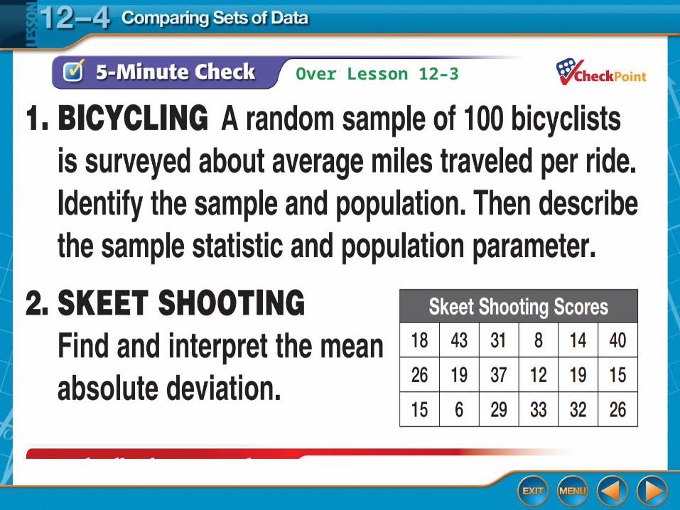
Over Lesson 12–3

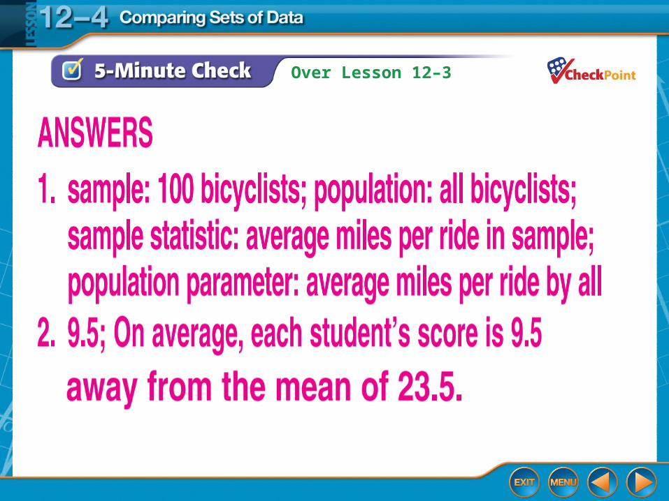
Over Lesson 12–3

Comparing Sets of Data

Lesson 12-4

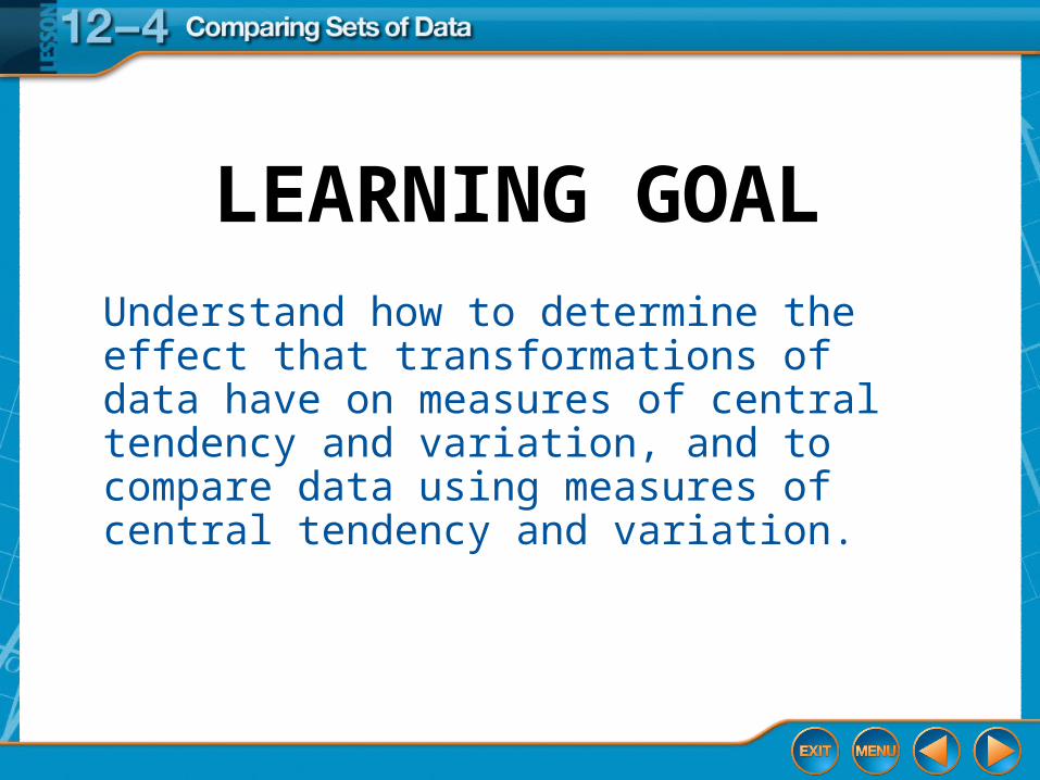
Understand how to determine the effect that transformations of data have on measures of central tendency and variation, and to compare data using measures of central tendency and variation.

LEARNING GOAL

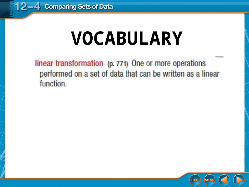
VOCABULARY

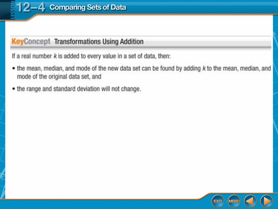
Transformation Using Addition

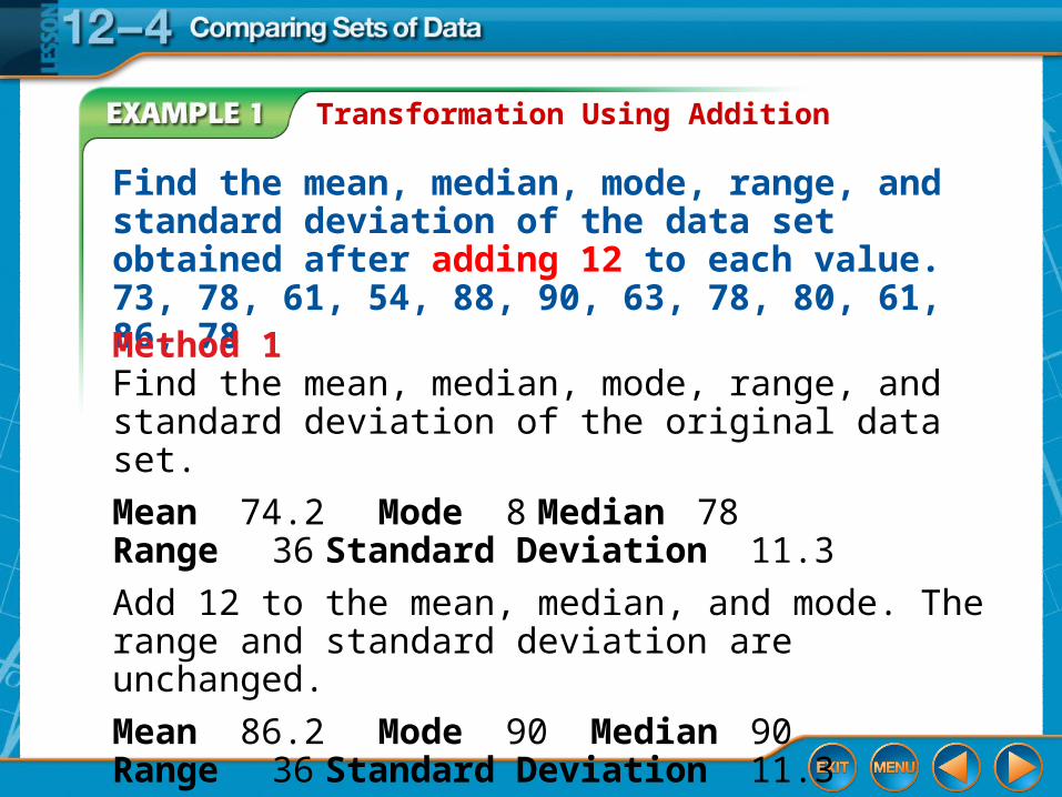
Find the mean, median, mode, range, and standard deviation of the data set obtained after adding 12 to each value.73, 78, 61, 54, 88, 90, 63, 78, 80, 61, 86, 78Method 1Find the mean, median, mode, range, and standard deviation of the original data set.

Mean 74.2 Mode 8 Median 78Range 36 Standard Deviation 11.3

Add 12 to the mean, median, and mode. The range and standard deviation are unchanged.

Mean 86.2 Mode 90 Median 90Range 36 Standard Deviation 11.3

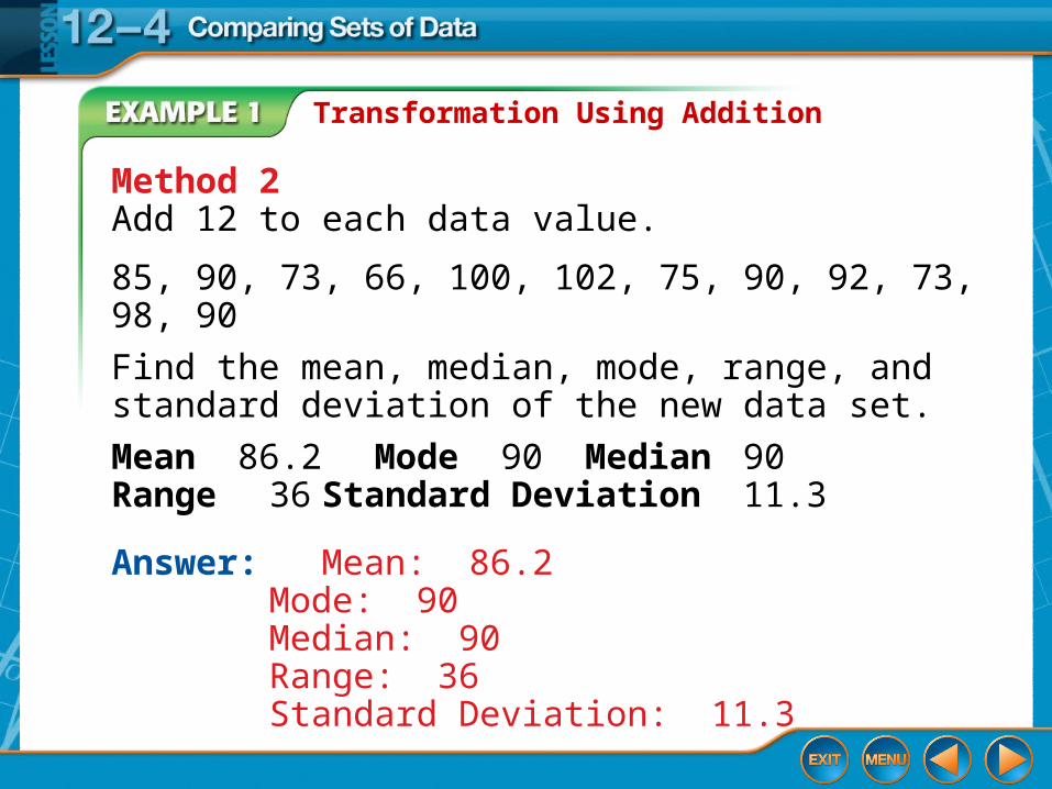
Transformation Using Addition

Method 2Add 12 to each data value.

85, 90, 73, 66, 100, 102, 75, 90, 92, 73, 98, 90

Find the mean, median, mode, range, and standard deviation of the new data set.

Mean 86.2 Mode 90 Median 90Range 36 Standard Deviation 11.3

Answer: Mean: 86.2Mode: 90Median: 90Range: 36Standard Deviation: 11.3

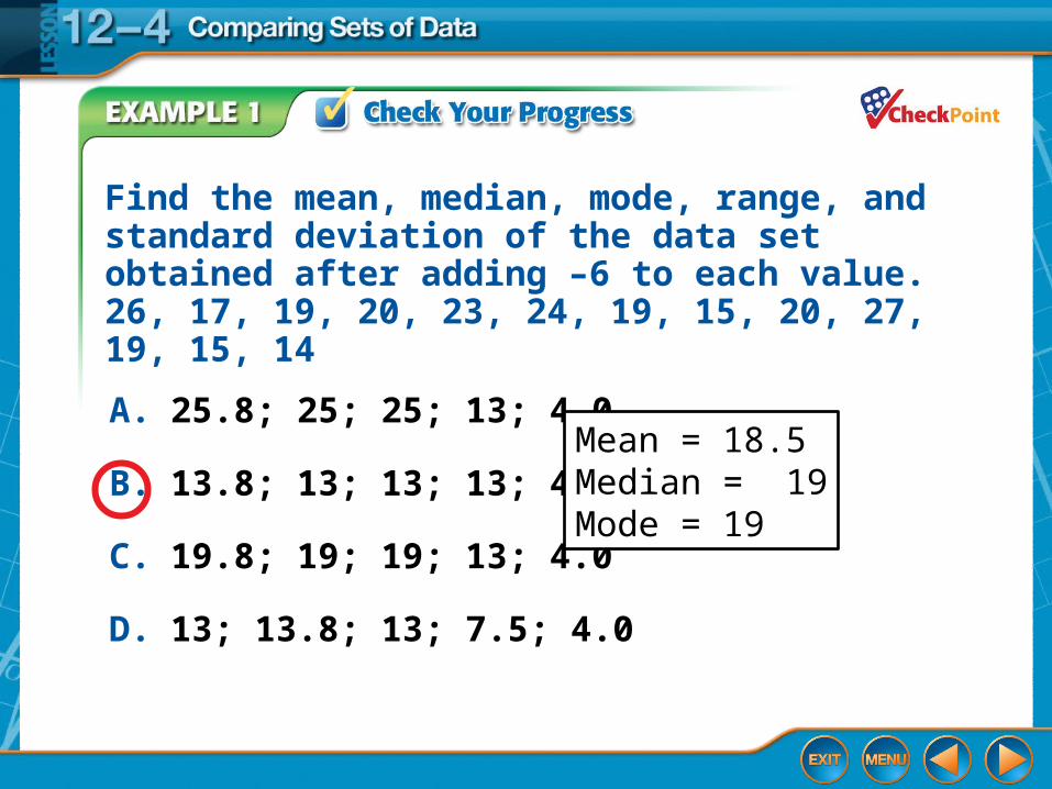
A. 25.8; 25; 25; 13; 4.0

B. 13.8; 13; 13; 13; 4.0

C. 19.8; 19; 19; 13; 4.0

D. 13; 13.8; 13; 7.5; 4.0

Find the mean, median, mode, range, and standard deviation of the data set obtained after adding –6 to each value.26, 17, 19, 20, 23, 24, 19, 15, 20, 27, 19, 15, 14

Mean = 18.5Median = 19Mode = 19

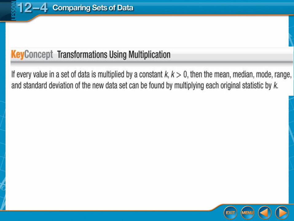
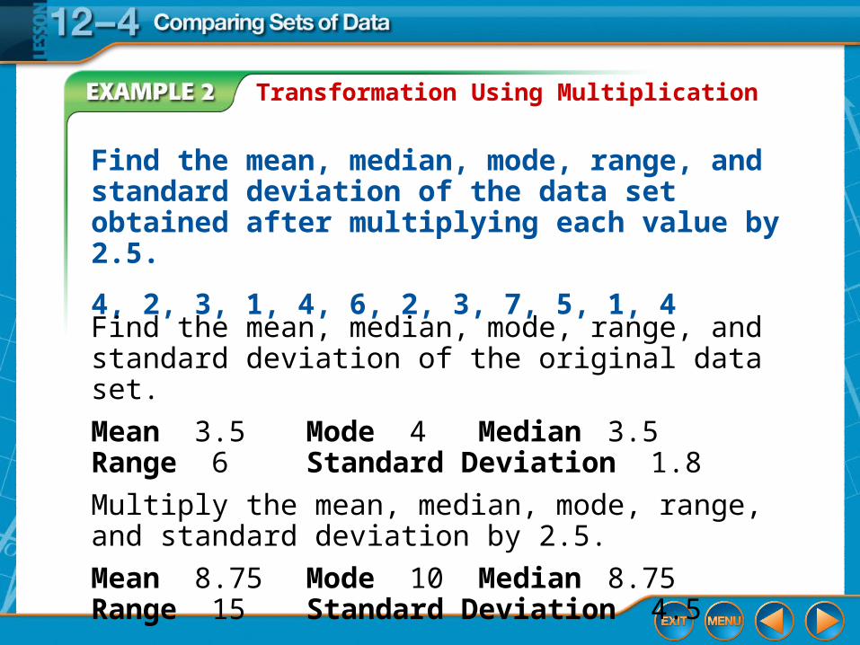
Transformation Using Multiplication

Find the mean, median, mode, range, and standard deviation of the data set obtained after multiplying each value by 2.5.

4, 2, 3, 1, 4, 6, 2, 3, 7, 5, 1, 4

Find the mean, median, mode, range, and standard deviation of the original data set.

Mean 3.5 Mode 4 Median 3.5Range 6 Standard Deviation 1.8

Multiply the mean, median, mode, range, and standard deviation by 2.5.

Mean 8.75 Mode 10 Median 8.75Range 15 Standard Deviation 4.5

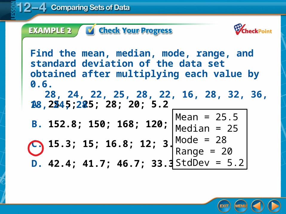
A. 25.5; 25; 28; 20; 5.2

B. 152.8; 150; 168; 120; 31.3

C. 15.3; 15; 16.8; 12; 3.1

D. 42.4; 41.7; 46.7; 33.3; 8.7

Find the mean, median, mode, range, and standard deviation of the data set obtained after multiplying each value by 0.6.

28, 24, 22, 25, 28, 22, 16, 28, 32, 36, 18, 24, 28

Mean = 25.5Median = 25Mode = 28Range = 20StdDev = 5.2

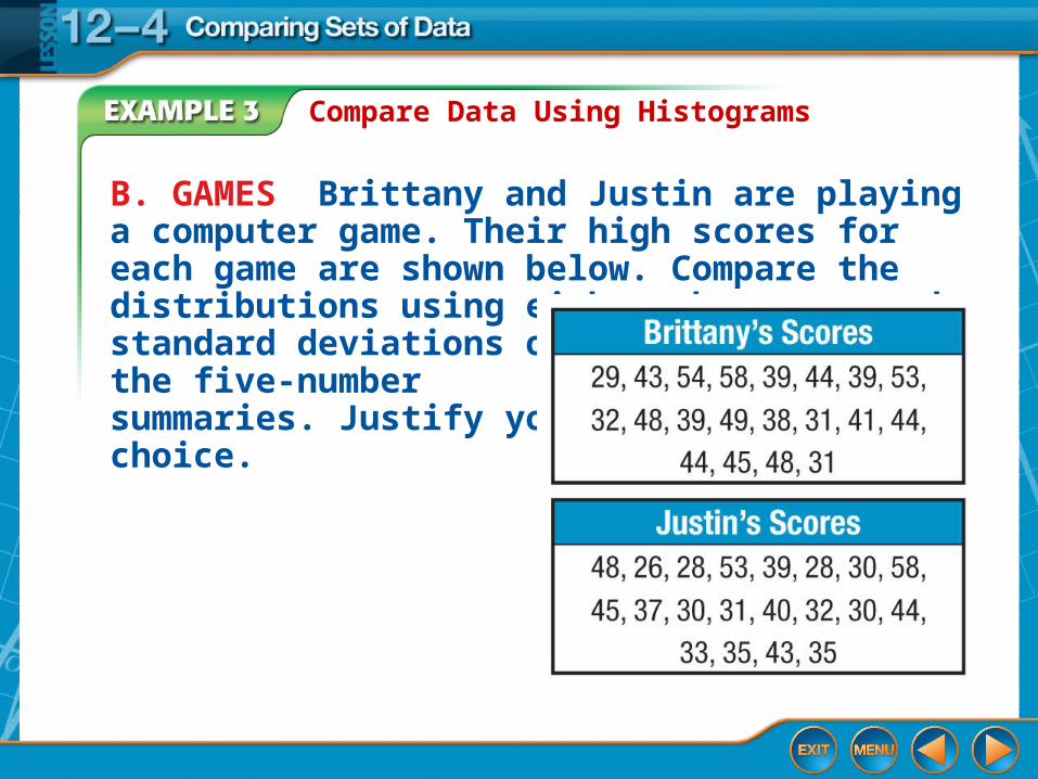
Compare Data Using Histograms

B. GAMES Brittany and Justin are playing a computer game. Their high scores for each game are shown below. Compare the distributions using either the means and standard deviations or the five-number summaries. Justify your choice.

Compare Data Using Histograms

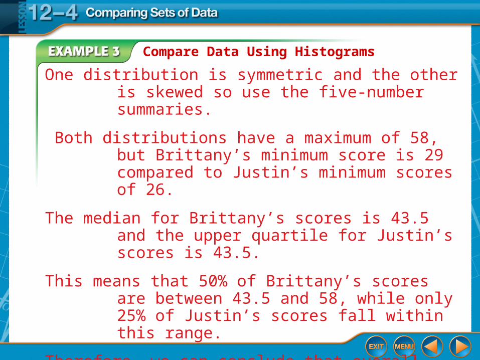
One distribution is symmetric and the other is skewed so use the five-number summaries.

Both distributions have a maximum of 58, but Brittany’s minimum score is 29 compared to Justin’s minimum scores of 26.

The median for Brittany’s scores is 43.5 and the upper quartile for Justin’s scores is 43.5.

This means that 50% of Brittany’s scores are between 43.5 and 58, while only 25% of Justin’s scores fall within this range.

Therefore, we can conclude that overall, Brittany’s scores are higher than Justin’s scores.

Compare Data Using Box-and-Whisker Plots

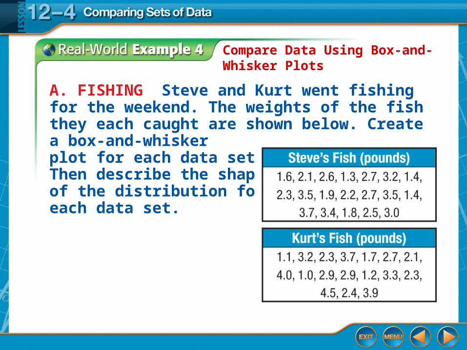
A. FISHING Steve and Kurt went fishing for the weekend. The weights of the fish they each caught are shown below. Create a box-and-whisker plot for each data set. Then describe the shape of the distribution for each data set.

Compare Data Using Box-and-Whisker Plots

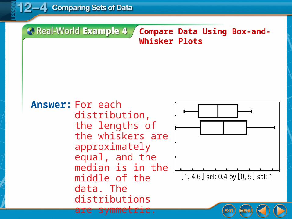
Answer: For each distribution, the lengths of the whiskers are approximately equal, and the median is in the middle of the data. The distributions are symmetric.

Compare Data Using Box-and-Whisker Plots

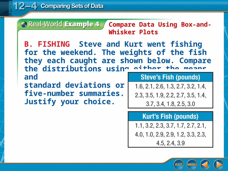
B. FISHING Steve and Kurt went fishing for the weekend. The weights of the fish they each caught are shown below. Compare the distributions using either the means and standard deviations or the five-number summaries. Justify your choice.

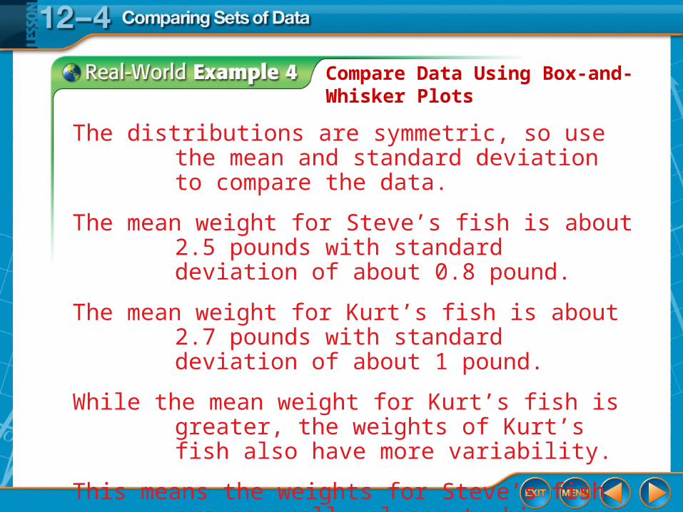
Compare Data Using Box-and-Whisker Plots

The distributions are symmetric, so use the mean and standard deviation to compare the data.

The mean weight for Steve’s fish is about 2.5 pounds with standard deviation of about 0.8 pound.

The mean weight for Kurt’s fish is about 2.7 pounds with standard deviation of about 1 pound.

While the mean weight for Kurt’s fish is greater, the weights of Kurt’s fish also have more variability.

This means the weights for Steve’s fish are generally closer to his mean than the weights for Kurt’s fish.

Homework

p. 776 #7 and 11