Embed Size (px)
Citation preview

Output-expanding collusion in
the presence of a competitive fringe
Juan-Pablo Montero and Juan Ignacio Guzmán∗
December 10, 2006
Abstract
Following the structure of many commodity markets, we consider a few large firms and a
competitive fringe of many small suppliers choosing quantities in an infinite-horizon setting
subject to demand shocks. We show that a collusive agreement among the large firms
may not only bring an output contraction but also an output expansion (relative to the
non-collusive output level). The latter occurs during booms and is due to the strategic
substitutability of quantities (we will never observe an output-expanding collusion in a
price-setting game). We also find that the time at which maximal collusion is most difficult
to sustain can be either at booms or recessions.
1 Introduction
In Table 1 we reproduce Orris C. Herfindahl’s Table 3 (1959, p. 115) with a summary of the
evolution of the so-called international copper cartel that consisted of the five largest firms and
operated during the four years preceding the Second World War. Herfindahl argues that the
cartel was successful in restricting output during the periods of low demand (denoted as Quota
status and associated to lower spot prices in the London Metal Exchange) but failed to extend
∗Montero ([email protected]) is Associate Professor of Economics at the Pontificia Universidad Católica deChile (PUC) and Research Associate at the MIT Center for Energy and Environmental Policy Research; Guzmán([email protected]) is PhD candidate at PUC and is currently visiting the Division of Economics and Businessof the Colorado School of Mines. We thank Claudio Agostini, Jeremy Bulow, Joe Harrington, Bill Hogan, JasonLepore, Salvador Valdés, Felipe Zurita and seminars participants for helpful discussions and comments. Thiswork was completed while Montero was visiting the Harvard’s Kennedy School of Government (KSG) under aRepsol YPF-KSG Research Fellowship. Montero also thanks Fondecyt (Grant # 1051008) for financial support.
1
such restrictions to the periods of high demand when the cartel and non-cartel firms returned
to their non-collusive output levels.1
Herfindahl’s description appears consistent with some existing collusion theories; in par-
ticular, with Rotemberg and Saloner’s (1986) prediction for the evolution of a cartel under
conditions of demand fluctuations in that collusive firms have more difficulties in sustaining
collusion during booms (i.e., periods of high demand).2 We advance a different behavioral
hypothesis in this paper. We posit that the large output expansions undertaken by cartel mem-
bers during the two booms (Jan.—Nov. 1937 and Oct.—Dec. 1938) may not necessarily reflect
a return to the non-collusive (i.e., Nash-Cournot) equilibrium but rather a continuation with
the collusive agreement in the form of a coordinated output expansion of cartel members above
their Nash-Cournot levels.3
The objective of this paper is to explore the conditions under which a collusive agreement,
if sustained, can take an output-expanding form at least during some part of the business cycle
and discuss its welfare implications. Although we do not run any empirical test, we will see
that the international copper cartel of 1935-39 as well as many of today’s commodity markets
appear to be good candidates in which such collusive characterization may apply. There are
basically two reasons for that. First, in these markets a firm’ strategic variable is its level of
production while prices are cleared, say, in a metal exchange. Second, collusive efforts, if any,
are likely to be carried out by a fraction of the industry (typically, the largest firms) leaving,
for incentive compatibility reasons, an important fraction of the industry (consisting mostly of
a large number of small firms) outside the collusive agreement but nevertheless enjoying any
eventual price increase brought forward by the collusive agreement (we will often refer to the
group of non-cartel firms as competitive fringe and to the group of potential cartel firms as
strategic or large firms).4
It is important to make clear that the possibility of having an output-expanding collusion,
1Walters (1944) also comments on the satisfactory operation of the cartel in that there is no indication thatsanctions for non-compliance were ever invoked.
2Rotemberg and Saloner’s (1986) prediction can change if we introduce imperfect monitoring (Green andPorter, 1984), a less than fully random demand evolution (Haltinwager and Harrington, 1991; Bagwell andStaiger, 1997), and capacity constraints (Staiger and Wolak, 1992).
3From reading some news of the time it appears that output expansions were indeed not totally left to eachcartel member’s unilateral actions but were somehow also orchestrated by the cartel (e.g., New York Times 1938,Oct. 11, pg. 37 and Oct. 18, pg. 37).
4Although the collusion literature usually assumes a structure of identical firms, this heterogeneous structurein which a few large firms compete with many smaller firms has long been recognized (Arant, 1956; Pindyck,1979).
2
and hence, lower prices, is totally unrelated to the idea that a cartel should prevent prices
going too high as to induce the development of a substitute product (or the discovery of new
mineral deposits) that can erode a fraction of the current demand.5 Besides that this can be
easily added to our model by including a probability of discovery increasing in prices (more
reasonably perhaps, in the average price of some period of time), our model is constructed
simply upon the presence of a known fringe of small suppliers that run and shut down their
production units so that at all moment the unit-cost of the marginal fringe firm is equal to the
equilibrium price. In addition and consistent with practical observation, we assume that the
entry or exit of large firms is a rare event.
Our results are entirely explained by market-interaction forces among existing players. As
demand expands, fringe members increase output with no regard of the effect that such increase
can have on the equilibrium price. Conversely, large firms do take into account the effect that
their output decisions have on the equilibrium price, and consequently, they "limit" their Nash-
Cournot output expansions as to accommodate for the fringe (price-taking) expansion. Because
of the strategic substitution between the output of fringe firms and that of large firms (Bulow et
al., 1985; Fudenberg and Tirole, 1984), it may indeed be optimal for the large firms to coordinate
in a joint output expansion beyond their Nash-Cournot levels. The price drop caused by the
strategic firms’ over-expansion is more than offset by their market share increase.
Whether it is optimal for the large firms to implement such an output-expanding collusion
as opposed to a traditional output-contracting collusion will ultimately depend on the fringe’s
(non-collusive) output, which in turn, will depend on cost differences between large and fringe
firms and on the magnitude of the demand shocks. One can always find fringe’s costs sufficiently
low (high) that it is optimal for strategic firms to implement an output-expanding (-contracting)
collusion for all possible realizations of demand. As we speculate for the copper cartel of 1935-39,
however, the more interesting case is that in which fringe costs generate both output-expanding
collusion during booms and output-contracting collusion during recessions.
One way to appreciate these results more fully it is to contrast them with those obtained
for a price-setting game with differentiated products.6 Think, for example, of a conventional
Hotelling linear city in which there are two large supermarkets in each extreme of the city and
5It is not new in the literature that the introduction of a competitive fringe can alter existing results. Rior-dan (1998), for example, shows how and when the presence of a (downstream) fringe reverses the well knownprocompetitive result of backward vertical integration by a downstream monopolist.
6 If products are perfectly homogeneous it is immediate that we can never have an output-expanding collusion.
3

a large number of small stores located downtown (i.e., in the middle of the city) competing
in prices.7 Following the arguments above, one could conjecture that for a fringe sufficiently
efficient that enjoys a large market share it may be optimal for the two supermarkets to co-
ordinate on jointly pricing below their non-collusive (Nash-Bertrand) levels and expand their
market share accordingly. It turns out this is never the case and the reason is the strategic
complementarity between prices charged by the strategic firms and by the fringe firms. If large
firms lower their prices, fringe firms’ equilibrium response is to lower theirs preventing large
firms from gaining market share.
The presence of an important fraction of non-cartel firms has also implications for cartel
firms’ ability to sustain the collusive outcome throughout the business cycle. Using the same
i.i.d. demand shocks of Rotemberg and Saloner (1986), we show that it is no longer true that
is more difficult for firms to sustain maximal collusion during booms than during recessions.
Depending on fringe’s costs relative to large firms’ and on the possible realizations of demand,
there will be cases in which it is more difficult for firms to sustain (maximal) collusion during
periods of low demand.
Because many commodity markets are characterized by the presence of a relatively large
fraction of small suppliers that will never enter into a collusive agreement, our results have
important policy implications. We cannot rule out, on theoretical grounds, that collusion
efforts by a group of large firms may be welfare enhancing when periods of output-contracting
collusion are followed by periods of output-expanding collusion.8 Based on the aggregate data
of Table 1, we illustrate this possibility in a numerical exercise for the copper cartel of 1935-39.
The rest of the paper is organized as follows. In the next section (Section 2) we present the
model and derive the (non-collusive) Nash-Cournot equilibrium. In Section 3 we present the
maximal collusive equilibrium and demonstrate the possibility of an output-expanding collusion
(we also demonstrate that the latter is never the case in a price-setting game). In Section 4, we
study the cartel stability along the business cycle. The numerical exercise based on the copper
7Note that in equilibrium all fringe firms that are called to produce charge the same price which is equal tothe unit-cost of the marginal fringe firm.
8 It is interesting to contrast these observations with recent events in the copper industry. Back in 2001 whenprices were at record low, the three largest firms in the industry made fairly simultaneous announcements ofsupply restrictions (either as lower production or inventory holdings) that were eventually carried out. Today,prices are at record high and some of the same firms are announcing very aggressive expansion plans. Obviously,in the absence of a more detailed empirical analysis we cannot tell whether these firms are engaged in some sortof tacit collusion or are rather optimally adjusting their supplies (including capacities and inventories) as theymove from one non-collusive equilibrium to another. Nevertheless, this paper should prove useful in structuringsuch an empirical test.
4
cartel data is in Section 5. Concluding remarks follow.
2 Oligopoly-fringe model
2.1 Notation
A group of n identical (strategic) firms (i = 1, ..., n) and a competitive fringe consisting of a
continuum of firms (indexed by j) produce some commodity in an infinite-horizon setting. At
the beginning of each period, firms simultaneously choose their production levels and the price
clears according to the inverse demand curve P (θ,Q) = θP (Q) with P 0(Q) < 0, where Q is
total production and θ ∈ [θ, θ] is, as in Green and Porter (1984), a multiplicative demand shockwhich is observed by all firms before they engage in production.9
Strictly speaking, only the n strategic firms have the possibility of choosing among different
production levels; a fringe firm’s decision is simply whether or not to bring its unit of output
to the market.10 The production cost of each strategic firm is Cs(qs) with C 0s(qs) > 0 and
C 00s (qs) ≥ 0 ("s" stands for strategic firm). The unit cost of fringe firm j is cj . The cj ’s,
which vary across firms, can be cost-effectively arranged along a marginal cost curve C 0f (Qf )
with C 00f (Qf ) > 0 and C 000f (Qf ) ≤ 0,11 where Qf =Rqfjdj is fringe firms’ output (we will use
capital letters to denote group production and small letters to denote individual production, so
strategic firms’ output is Qs =Pn
i=1 qsi and total output is Q = Qs +Qf ).
In some passages of the paper we will introduce, with little loss of generality, some sim-
plifying assumptions to the model that will allow us to better illustrate some of our results.
In particular, we will assume that P (Q) = a − bQ, that strategic firms have no production
costs and that the fringe’ aggregate marginal cost curve is C 0f (Qf ) = cQf , where a, b and c are
strictly positive parameters.12
9Below we explain how the results change under an additive shock (i.e., P (Q, θ) = P (Q) + θ).10 Including some fringe firms with output flexibility complicates the algebra with no implications in the re-
sults. It would be interesting, however, to study more formally the process of cartel formation when there areheterogenous firms.11 If anything, C0
f (Qf ) should be strictly concave (i.e., C000f (Qf ) < 0) capturing the practical observation that
fringe’s output is more elastic at higher prices (e.g., Crowson, 1999 and 2003).12That the costs of large firms are, on average, lower than the costs of smaller firms is not a bad assumption
–at least for mineral markets (Crowson, 2003). However, we do not need such assumption for our results; wecould have just worked with Cs(qs) = csqs at the expense of mathematical tractability.
5
2.2 The (non-collusive) Nash-Cournot equilibrium
A commonly used approach for finding the (static) Nash-Cournot equilibrium in the presence of
a competitive fringe is to first subtract the fringe’s supply function from the market demand to
obtain the residual demand faced by the large firms and then solve the non-cooperative game
among the large firms. This residual-demand approach, however, violates the simultaneous-
move assumption. It implicitly assumes a Stackelberg timing within in any given period: first,
large firms announce or choose their quantities; then and after observing large firms’ output
decisions, fringe firms choose their quantities. In the absence of technical reasons, this sequential
timing can only be supported by some degree of cooperation (i.e., collusion) among the large
firms that ensures that large firms will stick to their announcements or that they will not
move again together with the fringe.13 Without such cooperation, the static game necessarily
collapses into a simultaneous move game.14
Thus, the Nash-Cournot equilibrium of the one-period (simultaneous-move) game, i.e., the
equilibrium in the absence of any collusion efforts, is found by solving each firm’s problem as
follows
maxqsi
θP (qsi +Pj 6=i
qsj +Qf )qsi − Cs(qsi) for all i = 1, ..., n (1)
qfj =
1 if cj ≤ θP (Qs +Qf )
0 if cj > θP (Qs +Qf )for all j (2)
The n first-order conditions associated to (1) give us the best response of each strategic firm to
the play of all remaining firms. Similarly, (2) summarizes the best response of each fringe firm,
which is to produce as long as its unit cost is equal to or below the clearing price.
Given the symmetry of the problem, the equilibrium outcome of the one-period game is
given by
θP 0(Qnc)Qncs /n+ θP (Qnc)− C 0s(Q
ncs /n) = 0 (3)
θP (Qnc) = C 0f (Qncf ) (4)
13Suppose first that the sequential timing is the result of early production announcements by strategic firms.At the production stage, however, a strategic firm would like to deviate from its original announcement byproducing less. Suppose instead that the sequential timing is the result of early and observable production bystrategic firms (together with a commitment of no additional production). At the time fringe firms are called toproduce, however, a strategic firm will find it profitable to deviate from its commitment by bringing additionaloutput to the market.14One of the first oligopoly-fringe models that explicitily adopts this simultaneous-move assumption is Salant’s
(1976) model for the oil market.
6
where "nc" stands for Nash-Cournot or non-collusive equilibrium and Qnc = Qncs +Q
ncf . Solving
we obtain Qncs (θ) and Qnc
f (θ).15
3 Collusive equilibria
It is well known that in a infinite-horizon setting strategic firms may be able to sustain out-
comes in subgame perfect equilibrium that generate higher profits than the outcome in the
corresponding one-period game. Leaving for later discussion how easy or difficult is for firms
to sustain these collusive outcomes in equilibrium, or alternatively, assuming for the moment
that the discount factor δ (of strategic firms) is close enough to one,16 in this section we are
interested in finding the best collusive agreement for the strategic firms.
A natural point of departure in this simultaneous-move game is to compute what we call
the static monopoly outcome that results from taking the group of large firms as a single player
playing a one-period game against the fringe. The equilibrium is obtained from intersecting
the static reaction (best-response) function of the group of fringe firms with the "static best-
response function" of the group of large firms. Based on the works of Fudenberg and Levine
(1989) and Fudenberg, Kreps and Maskin (1990) on repeated games with long-run and short-
run players,17 one might argue that the static monopoly outcome is the best collusive agreement
attainable for the group of large firms if fringe firms are thought to be short-run players that
play only once and in addition have no means to learn about previous play. However, this is a
poor characterization of smaller firms in most commodity markets. As explained by Crowson
(1999), it is common in mineral markets to see smaller firms staying around for as long as
larger firms. It is also the case that smaller firms can learn about previous play without being
physically present, either through word-of-mouth or more likely from written sources.
More importantly, when fringe firms observe previous play it is natural to think that the
15The corresponding quantities for the simplified model are
Qncs =
nac
b[c(n+ 1) + θb]and Qnc
f =θa
c(n+ 1) + θb
Note that under this particular formulation ∂Qncs (θ)/∂θ < 0 and ∂Qnc
f (θ)/∂θ > 0; but we do not require theseproperties in any of our Propositions.16The discount factor of fringe firms is irrelevant since they always operate along their static best-response
function.17Fudenberg and Levine (1989) is not strictly a supergame as Fudenberg et al.(1990) and ours. They consider
a single long-run player and introduce a bit of uncertainty about its type. It does not seem straightforwardto us how to extend this incomplete information approach to the case of many long-run players each of themattempting to build reputation.
7
group of large firms can strictly improve upon the static monopoly outcome by following (equi-
librium) strategies that are dependent on the possible histories of the game. In other words,
the expectations of fringe firms as to what the large firms will produce are now sensitive to
previous play of large firms which in turn allows the group of large firms to credibly communi-
cate its commitment to (profitably) depart from the static monopoly outcome.18 We will refer
to the most preferred of these dynamic outcomes as the maximal collusive agreement. Before
describing its properties, we will present the static monopoly outcome because it will help us
to more easily convey the intuition behind our main result.
3.1 Static monopoly outcome
The static best-response function of fringe firms,19 which we denote by the aggregate function
Q∗f (Qs), is implicitly given by θP (Qf + Qs) = C 0f (Qf ). On the other hand, the static best-
response function of the group/cartel of large firms to an aggregate play of Qf by the fringe
firms is given by
Q∗s(Qf ) = argmaxQs
{θP (Qs +Qf )Qs − nCs(Qs/n)}
Given a discount factor close enough to one, the stability of the cartel of large firms is subgame
perfect and it is assumed here that this is correctly anticipated by fringe firms. Hence, the
static monopoly outcome is obtained from the intersection of Q∗f (Qs) and Q∗s(Qf ). Denoting
by Q0s and Q0f the corresponding equilibrium quantities, we have
θP 0(Q0)Q0s + θP (Q0)− C 0s(Q0s/n) = 0 (5)
θP (Q0) = C 0f (Q0f ) (6)
18Unlike in Fudenberg and Levine (1989) where there is a single long-run player, here we have two or morelarge firms which allow them by the threat of falling into a price war, as in Gul (1987) for the durable-goodduopolists, to build commitment despite fringe firms do not observe previous play. This would require, however,to impose fixed beliefs as to what fringe firms expect large firms to produce in each period. We could just assumethat, but it is more natural to us to think that fringe firms’ beliefs are not (exogenously) fixed but rather sensitiveto past play.19Note that since fringe firms are infinitesimally small they always play along their static best-response curve
regardless of their life horizon (Mailath and Samuelson, 2006).
8

where Q0 = Q0s + Q0f .20 Solving we obtain the static-monopoly equilibrium quantities Q0s(θ)
and Q0f (θ).21
By comparing equilibrium conditions (3)—(4) with (5)—(6), it holds that
Lemma 1 Q0s(θ) < Qncs (θ) and P (Q0(θ)) > P (Qnc(θ)) for all θ.
Proof. Straightforward since P 0(Q) < 0 and n ≥ 2.This is the conventional view regarding the operation of a cartel in that it always reduces
output to lift prices. In the presence of a competitive fringe there is a caveat, however. When
the fringe’s output is large enough, it may be optimal for the large firms to stick to the non-
collusive equilibrium (and fringe firms anticipate that). From conventional monopoly theory,
we would say that in such cases large firms do not want to restrict output any further because
they face a too elastic (residual) demand.
This possibility can be easily illustrated for our simplified (i.e., linear) model. Let π0s and
πncs be the strategic firm’s profits under static monopoly and Nash-Cournot, respectively.22 It
can be shown that
π0s(θ) > πncs (θ)⇐⇒ θ < (√n− 1)c/b ≡ θ̃ (7)
Expression (7) indicates that for demand shocks sufficiently large it is optimal for large firms to
follow Nash-Cournot strategies instead of static monopoly pricing. Note that the smaller the
value of c and/or n the fewer the times at which large firms want to (statically) collude. The
reason is that in this example large firms’ (non-collusive) market share is increasing in n and
c.23
20We have not been explicit about what happens when a large firm deviates from the (collusive) equilibriumpath. A reasonable (subgame perfect) punishment path is a return to Nash-Cournot but with fringe firms playing,on aggregate, Q0
f (not Qncf ). This is because in this "one-shot game" fringe firms’ beliefs are fixed in that they
expect the large group to always play Q0s. There are no deviations in equilibrium, however.
21For the simplified model these quantities are
Q0s =
ac
b(2c+ θb)and Q0
f =θa
2c+ θb
22The profits for the simplified model are
πncs =θ
b
·ac
c(n+ 1) + θb
¸2and π0s =
θ
nb
·ac
2c+ θb
¸2
23That large firms may find it optimal to remain at their Nash-Cournot levels is not unique to the quantitycompetition assumption. In fact, in the Hotelling-city example of the introduction the Nash-Bertrand prices andthe static monopoly prices are the same.
9
3.2 Maximal collusion
Assuming that all players acting at date t have observed the history of play up to date t,
it is possible to construct history-dependent strategy profiles with payoffs for the large firms
that are strictly higher than those under the static monopoly outcome (and easier to sustain).
While the latter is one of the multiple possible equilibria in this repeated game, here we are
interested in finding the maximal collusive agreement, that is, the one that gives large firms the
highest attainable payoff for a discount factor close enough to one. Let Qms and Q
mf denote the
(aggregate) quantities corresponding to the maximal collusive equilibrium.
Since strategic firms are symmetric and there are no economies of scale, it is optimal for
each strategic firm to produce qmsi = Qms /n, hence
Qms = argmax
Qs
{θP (Qs +Qf (Qs))Qs − nCs(Qs/n)} (8)
where Qf (Qs) is the fringe’s equilibrium response to Qs, which is implicitly given by
θP (Qf +Qs) = C 0f (Qf ) (9)
Replacing Qf (Qs) from (9) into (8), the strategic firms’ maximal collusive outcome solves
C 00f (Qmf )θP
0(Qm)
C 00f (Qmf )− θP 0(Qm)
Qms + θP (Qm)− C 0s(Q
ms /n) = 0 (10)
θP (Qm) = C 0f (Qmf ) (11)
where Qm = Qms + Qm
f . Solving we obtain the collusive equilibrium strategies Qms (θ) and
Qmf (θ).
24 ,25
Note that having Qf as a function of Qs in (8) resembles a Stackelberg (static) game but
it is only because in this repeated game large firms anticipate and use fringe firms’ equilibrium
24For the simplified model the equilibrium quantities are
Qms =
a
2band Qm
f =θa
2(c+ θb)
Note that ∂Qmf (θ)/∂θ > 0.
25We have been silent about the implementation of the (maximal) collusive agreement. We can think of thefollowing set of (symmetric) trigger strategies (which depend on the realization of θ): In period 0, strategic firm iplays Qm
s /n and fringe firms play, on aggregate, Qmf . In period t, firm i plays Qm
s /n if in every period precedingt all strategic firms have played Qm
s /n; otherwise it plays Qncs /n. Fringe firms, on the other hand, play Qm
f in tif in every period preceding t all strategic firms have played Qm
s /n; otherwise they play Qncf .
10
response in constructing its optimal action and not because some first-mover advantage. By
comparing equilibrium conditions (3)—(4) with (10)—(11) we can establish
Proposition 1 There is a level of demand θ̂ for which Qm(θ̂) = Qnc(θ̂) ≡ Q̂(θ̂), Qmf (θ̂) =
Qncf (θ̂) ≡ Q̂f (θ̂) and Qm
s (θ̂) = Qncs (θ̂) ≡ Q̂s(θ̂). This (unique) level of demand is found by
replacing the definitions of Q̂(θ̂) and Q̂f (θ̂) into θ̂ = −(n− 1)C 00f (Q̂f (θ̂))/P0(Q̂(θ̂)) and solving.
In addition, if θ is greater (lower) than θ̂, then Qm is greater (lower) than Qnc.
Proof. See the Appendix
This proposition opens up the possibility for an output-expanding collusion provided that θ̂
exists, i.e., θ̂ ∈ [θ, θ], which will always be the case for C00f (·) sufficiently small. More interesting,the collusive agreement may include both output expansions (above Nash-Cournot levels) during
periods of higher demand (i.e., θ > θ̂) and output contractions during periods of lower demand
(i.e., θ < θ̂). In providing more intuition for our results, it is useful to present the following
result first
Proposition 2 If the strategic and fringe firms were competing in prices (i.e., upward sloping
reaction functions), it would have been never optimal for the strategic firms to jointly price
below their (non-collusive) Nash-Bertrand price levels.
Proof. See the Appendix.
Propositions 1 and 2 indicate that an output-expanding, or equivalently, a price-reducing
collusion, is only a possibility under quantity competition and never under price competition.
This observation can be understood as the balance of two effects that in price competition work
in the same direction while in quantity competition work in opposite directions. We can think
of the first effect as a static effect. In a one-shot simultaneous-move game the best collusive
outcome for the group of large firms is the static monopoly outcome of Section 3.1 which
always have large firms reducing output (increasing prices) below (above) their Nash-Cournot
(-Bertrand) levels.
The second effect is a dynamic effect that comes from the fact that in a repeated game the
group of large firms can use history-dependent strategies to credibly build commitment towards
the implementation of a better outcome than the one-shot simultaneous-move outcome.26 Un-
like the static effect, the dynamic effect works in opposite directions depending on the type of
26This is equivalent to the reputation effect of Fudenberg and Levine (1989) for the case of a single (long-run)player playing a simultaneous-move stage game against a sequence of short-run opponents (i.e., that play onlyonce).
11
competition and is because of the strategic substitutability of quantities versus the strategic
complementarity of prices (Bulow et al., 1985; Fudenberg and Tirole, 1984).
When firms compete in prices and large firms jointly lower (increase) their prices, fringe
firms’ equilibrium response is to lower (increase) theirs. Note from eq. (18) in the Appendix
that ∂pf (ps1, .., psn)/∂psi > 0 for all i, where pf and psi are, respectively, the prices charged
by fringe firms and strategic firm i. Knowing this, the dynamic effect makes large firms to
price even higher relative to the static-monopoly outcome. On the other hand, when firms
compete in quantities and large firms jointly increase their productions, fringe firms’ equilibrium
response is not to increase their quantities but to reduce them (note from (9) that Q0f (Qs) =
θP 0(Qm)/[C 00f (Qmf )− θP 0(Qm)] < 0). The dynamic effect now makes strategic firms to expand
their production taking advantage of fringe’s contracting response.27
Whether it is optimal for strategic firms (competing in quantities) to follow an output-
expanding collusion or not, at least for some levels of demand, will depend on whether the
dynamic effect dominates the static effect. Provided that θ̂ exists, Proposition 1 establishes
that for θ < θ̂ the static effect dominates while for θ > θ̂ the dynamic effect dominates. The
reason why the dynamic effect dominates the static effect as demand raises is because fringe’s
(non-collusive) output is increasing in θ.28 More interestingly, one can imagine situations in
which a collusive agreement among the large firms can increase overall welfare as long as periods
of output-contracting collusion are followed by periods of output-expanding collusion.29
Let illustrate some of these results for our simplified model (i.e., P (Q) = a− bQ, Cs(qs) = 0
and C 0f (Qf ) = cQf ). From Proposition 1, the level of demand for which the optimal collusive
outcome coincides with the Nash-Cournot outcome is θ̂ = (n−1)c/b.30 Consequently, a collusiveagreement among the strategic firms will lead to higher output (and, hence, to lower prices)
27To understand this further, think of a holding company that owns all of the large firms. The (Nash-Cournot)outcome of the one-period simultaneous-move game between this holding company and the fringe is the staticmonopoly outcome derived in Section 3.1. In a simultaneous-move repeated game and where fringe firms observeall previous play the holding company can do strictly better by committing to a larger (Stackelberg) quantity inall possible demand realizations (provided that the discount factor is close enough to one).28Note that for the existence of θ̂ we do not require that the fringe’s (Nash-Cournot) market share be also
increasing in θ. In fact, one can find situations in which the fringe’s market share is shrinking with θ, yet, thelarge firms want to implement an output-expanding collusion (we did so in the simplified model for c relativelylarge and Cs(qs) = csq
2s with cs > 0).
29Bulow et al. (1986) make a closely related point when they ask whether "little competition is a good thing."The answer depends on whether the entry of a small fringe will cause the incumbent monopolist to expandor contract output: entry is a good thing with strategic complements and is welfare reducing with strategicsubstitutes.30Note from expression (7) that θ̃ < θ̂, which may call some readers’ attention. The reason is that the static
effect is still present beyond θ̃ and is only at θ̂ when is exactly offset by the dynamic effect.
12
as long as θ > (n− 1)c/b; a condition that can be conveniently expressed in terms of Cournotmarket shares as follows (see footnote 15 for the values of Qnc
f and Qncs )
θ >(n− 1)c
b⇐⇒ Qnc
f
Qnc>
n− 12n− 1 (12)
When the fringe’s market share in the Nash-Cournot equilibrium is larger than (n−1)/(2n−1),the group of strategic firms faces such a elastic "residual" demand that it is optimal for them
to coordinate in an output-expanding collusive agreement.
Since the fringe’s market share is increasing in θ and decreasing in c, condition (12) is more
likely to hold when the demand is large and the fringe is more efficient (i.e., has low c). For
example, if n = 2 the collusive agreement will take the conventional output-contracting shape
only when the fringe’s market share is less than 1/3. More generally, any time the fringe’s
Cournot market share is above 1/2 the collusive agreement is to expand output above Cournot
levels regardless of the number of firms. These results have also implications for understanding
the shape that a collusive agreement can take among a subset of (heterogeneous) strategic
firms. The fewer the strategic firms taking part in the collusive agreement the more likely it
will contain at least some periods of (collusive) output expansion.
Before turning into the sustainability of the collusive agreement, there are two assumptions
that deserve some discussion. First, if we relax the concavity assumption of the fringe’s marginal
cost (i.e., C 000f (Qf ) ≤ 0) and let it become mildly convex none of our results would change (seeProof of Proposition 1). If, however, we depart from practical observation and let the fringe’s
supply function C 0f (Qf ) be highly inelastic above certain price level, then θ̂ may not exist.
Second, we have seen that with multiplicative demand shocks collusion can bring both
output-contraction during recessions and output-expansion during booms. With additive de-
mand shocks, i.e., P (Q, θ) = P (Q)+θ, the condition that separates output-contracting collusion
from output-expanding collusion reduces to whether −(n−1)C 00f /P 0 is greater or lower than theunity. If both the fringe’s supply function C 0f (Qf ) and the demand function P (Q) are linear,
the collusive agreement would exhibit either output contractions or expansions throughout the
entire business cycle, which appears little realistic. If, on the other hand, the elasticity of the
fringe’s supply function is increasing in prices (i.e., C 000f (Qf ) < 0), we could again have a mixed
collusive regime with output contraction for θ < θ̌ and output expansion for θ > θ̌, where θ̌
solves −(n− 1)C 00f (Qf (θ̌))/P0(Q(θ̌)) = 1. It is possible that in reality shocks are best modeled
13
as a combination of both specifications.31
4 Collusion over the business cycle
We have characterized the maximal collusive agreement but said nothing on how difficult is for
the strategic firms to sustain such an agreement under varying demand conditions. The question
of whether is more difficult for firms to sustain collusion during booms than during recessions
(or vice versa) has received a great deal of attention in the literature after the pioneers works
of Green and Porter (1984) and Rotemberg and Saloner (1986). Since our intention is not to
provide a discussion of how all existing results could change with the introduction of a (large)
fringe, we follow Rotemberg and Saloner’s (1986) in that demand is subject to (observable) i.i.d.
θ shocks. We also assume that all (strategic) firms use the same factor δ ∈ (0, 1) to discountfuture profits.
For maximal collusion to be sustained throughout the business cycle it must hold for all θ
and for each strategic firm that the profits along the collusive path be equal or greater than the
profits from cheating on the collusive agreement and falling, thereafter, into the punishment
path, that is
πm(θ) + δV m ≥ πd(θ) + δV p (13)
where V m = Eθ[πm(θ)]/(1−δ) is the firm’s expected present value of profits along the collusive
path, πd(θ) is the profit obtained by the deviating firm in the period of deviation and V p is
the firm’s expected present value of profits along the punishment path. Although in principle
the punishment path can take different forms (which may include return to collusion after
some period of time), reversion to Nash-Cournot appear to us as most reasonable, particularly
because of the fringe presence. Expression (13) adopts this view,32 so V p = Eθ[πnc(θ)]/(1− δ).
It is important to notice that the direction of the deviation from the collusive agreement vary
along the business cycle. If the deviation occurs sometimes during the output-contracting phase
of the collusive agreement (i.e, when θ < θ̂), the optimal deviation is to increase output (i.e.,
move in the Nash-Cournot direction). But if deviation occurs sometimes during the output-
expanding phase (i.e, when θ > θ̂), the optimal deviation is to reduce output below the collusive
level. This invites us to speculate, at least in theory, about the possibility that a fringe firm
31See also Turnovsky (1976) for a technical discussion on the use of multiplicative shocks as opposed to additiveshocks.32We also consider the optimal penal codes of Abreu (1986, 1988) and find no qualitative changes in our results.
14
could sabotage one of the strategic firms’ production sufficiently enough as to force the latter
to implement an (optimal) deviation and, hence, trigger a return to Nash-Cournot prices.33
We can now use (13) to obtain the discount factor function δ(θ) = (πd(θ)−πm(θ))/(V m−V p)
that establishes the minimum discount factor needed to sustain maximal collusion at θ provided
that maximal collusion is sustained at all other θ’s.34 Then, the critical demand level θc at
which becomes most difficult for firms to sustain maximal collusion can be defined as θc =
argmaxθ δ(θ). In other words, firms can sustain maximal collusion throughout the business
cycle only if δ ≥ δ(θc).
To facilitate the exposition, let us adopt for a moment, the simplifying assumptions of linear
demand and costs, which will allows us to obtain tractable expressions for πd(θ) and πm(θ).
Solving we obtain35
δ(θ) =θ[(n− 1)c− θb]2
(c+ θb)2K (14)
where K = a2/16n2b(V m − V p).
The function δ(θ) is plotted in Figure 1, which exhibits a local maximum at 0 < θ1 < θ̂ and
a global minimum at θ̂ –when maximal collusion reduces to the Nash-Cournot outcome. Note
that δ(θ) has been drawn without paying attention to the fact that the support of θ is some
subset [θ, θ] of <+. Despite both V m and V p depend on the actual support (and distribution)
of θ, they enter as constant terms in (14), so changes in the support (and/or distribution)
of θ will only scale δ(θ) up or down with no effects on the discussion that follows (e.g., θ1
is independent of θ and θ). More importantly, depending on the values of θ and θ one can
construct cases in which the critical time is either at booms (e.g., [θ = 0, θ = θ1], [θ = θ̂, θ > θ̂])
or at recessions (e.g., [θ = θ1, θ = θ̂]). The latter example is most interesting because even if we
restrict attention to output-contracting collusion, that is, θ ≤ θ̂, we do not need invoke Green
and Porter’s (1984) imperfect monitoring to generate price wars at recessions.36
33Obviously, the incentive for a strategic firm’s to sabotage the production of another strategic firm are alwayssmaller than the incentives to deviate from the collusive aggrement itself because the sabotage (regardless ofwhether it is detected or not by the affected firm) involves the simultaneous deviation of two firms which isalways less profitable than the deviation of a single firm.34 It is not difficult to show for the simple model that sustaining maximal collusion is easier than sustaining
the static monopoly outcome. Since πm(θ) > π0(θ), it sufficies to show that πd(θ) is smaller than the one-periodprofit from deviating from the monopoly outcome. After some algebraic manipulation we obtain that this holdsfor θ ≤ (√n− 1)c/b, but from Lemma 2 we know this is the relevant range.35πd(θ) = θb[qd(θ)]2, where qd(θ) = a[c(n + 1) + θb]/4nb(c + θb) is the optimal deviation when each of the
remaining strategic firms are playing Qms /n.
36The Bagwell and Staiger’s (1997) model of serially correlated demand shocks is also able to generate pricewars at recessions for some parameter values.
15
The above discussion extends to the general model in that we can establish
Proposition 3 The time at which is more difficult for large firms to sustain maximal collusion
can be either at booms or recessions.
Proof. See the Appendix
The above result entirely hinges on the fact that there exists a demand level θ̂ at which the
collusive and the non-collusive outcomes are indistinguishable, so collusion for any nearby θ is
easily sustained. As we increase fringe’s costs, θ̂ moves to the right (see Proposition 1) and
eventually falls outside the support of θ. In the limit, when fringe’s costs are so high that its
market share goes to zero, we return to Rotemberg and Saloner’ (1986) prediction that in the
absence of fringe firms collusion is more difficult to sustain during booms (i.e., at the largest
θ).37
5 Welfare: A numerical exercise
One of the main implications of our results is that the effect of collusion on welfare is to be
signed on a case-by-case basis. If Herfindahl’s behavioral hypothesis is correct, the copper cartel
of 1935-39 had an unambiguous negative impact on welfare. But this is not necessarily so if one
believes the cartel was also able to sustain collusion during booms. To illustrate this possibility,
consider the following numerical exercise. Assume that the cartel was able to sustain maximal
collusion in each of the six periods described in Table 1 and use the (aggregate) price and
quantity data of each of those periods to recover cost and demand parameters. Then, use these
parameters to predict what would have been the non-collusive equilibrium in each period.
In carrying out the exercise, we assume that (i) the five cartel members are identical, (ii)
the demand in period t = 1, ..., 6 is Pt(Qt, θt) = θt(a − bQt), (iii) the marginal cost function
of each of the cartel members is cstqγst, and (iv) the fringe’s marginal cost function is cftQ
ηft.
The parameters to be estimated are θt, a, b, cst, γ, cft, η. We have more parameters than
equilibrium equations so we are forced to make some (reasonable) arbitrary selections. We set
b = 0.7 to work with demand elasticity numbers around −0.35; similar to those in Agostini(2006) and the studies cited therein. In addition, we set γ = η = 0.4. We do not have a good
37Strictly speaking Rotemberg and Saloner (1986) show that in a quantity-setting game (with no fringe) it isnot always the case that collusion is more difficult to sustain at booms. It is the case though when demand andcosts are linear. In fact, in the limiting case of no fringe eq. (14) reduces to limc→∞ δ(θ) = θ(n− 1)2K, whereK = a2/16n2b(Vm − V p) and V m and V p correspond to the no-fringe values.
16
reason to differentiate between γ and η and these numbers produce less variation among the
ckt’s (k = s, f), which we think should not vary much in a four-year period. Besides, lower
numbers (e.g., γ = η = 0.1) produce the unreasonably scenario of output-expanding collusion
at all periods while higher numbers (e.g., γ = η = 0.7) result not only in wide variation among
ckt’s but also in some negative cft’s. We also normalize the demand shocks to the apparently
largest shock, that is, θ3 = 1.
Results, which are merely for illustrative purposes and not aimed at testing hypothesis, are
reported in Table 2. The next three columns following the period column show demand and
costs parameters for the six periods.38 In the fifth, sixth and seventh columns we reproduce
the (assumed) maximal collusion levels of Table 1 (quantities are again at their annual rates)
to facilitate the comparison with the hypothetical Nash-Cournot levels of the following three
columns. As predicted by our theory, the non-collusive prices are lower during recessions (t =
1, 2, 4 and 6) but higher during booms (t = 1 and 5). Furthermore, the average non-collusive
price (weighted by the number of months in the period) is almost equal to the average collusive
price (10.3 vs. 10.4). Provided that collusion prices are less volatile and that a one cent off
during booms add more to consumer surplus than a one cent off during recessions, it may well
be that the copper cartel of 1935-39 did not have a negative impact on welfare but the opposite.
Obviously, this is just an hypothesis that has yet to be tested econometrically.
6 Final remarks
Following the structure of many commodity markets, we have studied the properties of a col-
lusive agreement when this is carried out only by the largest firms of the industry. We have
found that as the (non-collusive) output of the noncartel firms expands, it may be optimal for
the cartel to jointly produce above their non-collusive levels. Consequently, we cannot rule out,
at least in theory, the possibility of a welfare-enhancing collusive agreement in which periods
of output-contracting collusion are accompanied by periods of output-expanding collusion.
We also found that due to the presence of a significant fraction of noncartel firms (i.e., fringe
firms), we do not need Green and Porter’s (1984) imperfect information to generate price wars
in recessions (i.e., procyclical pricing). More generally, it may be equally difficult for large firms
38Notice the variation of the cartel firms’ cost parameters (i.e., cs’s), particularly the low numbers in t = 3 and5. Besides indicating that even lower numbers (i.e., higher variation) would have resulted had we assumed returnto Nash-Cournot during these two booms, it may be that these low numbers reflect an asymmetric expansionwith greater participation of lower cost firms.
17

to sustain maximal collusion during booms than during recessions. It would be, nevertheless,
interesting to extend the model to the case of imperfect information.
There are other theoretical extensions worth pursuing. So far we have assumed that large
firms have sufficient flexibility to expand production as needed. While this seems to be less
of a problem for the international copper cartel of 1935-39 thanks to the excess capacity left
by the 1929-33 world contraction,39 the introduction of capacity constraints is likely to affect
the properties of the collusive agreement (Staiger and Wolak, 1992). One can go even further
and study altogether collusion in output and capacity (recall that in these markets firms are
constantly expanding their capacities to cope with depreciation and new demand). This surely
opens up the possibility for a capacity-expanding collusion even when firms set prices in the
spot market. In addition to capacity constraints, the opportunity of forward contracting part
of future production can also have implications for the collusive agreement (Liski and Montero,
2006).
Finally, it would be most interesting to carry out an empirical analysis of the copper cartel
of 1935-39 along the works of Porter (1983) for the JEC railroad cartel and test for periods of
output-expanding collusion. One important difference with these previous studies is that we
not only need to econometrically distinguish between regimes of (output-contracting) collusion
and price wars (i.e., return to Nash-Cournot) but perhaps more difficult between regimes of
output-expanding collusion and price wars.
Appendix
Proof of Proposition 1: The first part is straightforward. For Qm = Qnc we need
C 00f (·)θP 0(·)/(C 00f (·) − θP 0(·)) = θP 0(·)/n which rearranged leads to θ = −(n − 1)C 00f (·)/P 0(·).For the second part, we need to show that if we are at θ = θ̂ and let θ go up by a marginal
amount, say, to θ0, the term C 00f /(C00f − θP 0) in (10) suffers a greater fall (recall that P 0 < 0)
than the term 1/n in (3). If this is so, Qms (θ
0) must be larger than Qncs (θ
0) (and, hence, Qm(θ0)
larger than Qnc(θ0)) for both (3) and (10) to continue holding at θ0 = θ̂ + dθ. Therefore, we
need to showd
dθ
ÃC 00f (Q
mf (θ))
C 00f (Qmf (θ))− θP 0(Qm(θ))
!< 0 (15)
39 It would also be less of a problem if large firms manage, as in mineral markets, an in-house inventory to bebuilt up during recessions and withdrawn during booms.
18
Totally differentiating and rearranging, condition (15) reduces to
−C 000f · θP 0 · (dQmf (θ)/dθ) + C 00f · (P 0 + θP 00 · (dQm(θ)/dθ)) < 0
But since C 000f (Qf ) ≤ 0 by assumption, P 0 + θP 00 · (dQm(θ)/dθ) ≡ d[θP 0(Qm(θ))]/dθ < 0 (recall
that limθ→∞θP 0(Q) = −∞), and both dQ(θ)/dθ and dQf (θ)/dθ are, by construction, positive
for all θ, expression (15) holds, which in turn implies that dQm(θ)/dθ|θ=θ̂ > dQnc(θ)/dθ|θ=θ̂.40
It remains to show that θ̂ is unique. Suppose the contrary that there exists some θ̌ 6= θ̂ for
which Qm(θ̌) = Qnc(θ̌). But if (15) holds for θ̂ it cannot simultaneously hold for θ̌, which would
be a contradiction.
Proof of Proposition 2: Consider a group of n strategic firms (i = 1, ..., n) and a com-
petitive fringe consisting of a continuum of firms (indexed by j) engaged in a simultaneous
price-setting game of infinite horizon. Strategic firms produce differentiated goods at the same
cost Cs(qsi). Fringe firms produce a homogenous good according to the aggregate marginal cost
curve C 0f (Qf ) (as before, a fringe firm’s unit-cost is denoted by cj). Strategic firm i’s demand
is qsi ≡ Dsi(psi,p−si, pf ), where p−si is the vector of prices charged by the remaining strategic
firms and pf is the price charged by all fringe firms (it should be clear that in equilibrium pf will
be equal to the unit-cost of the most expensive fringe firm that entered into production, that no
fringe firm with a unit-cost equal or lower than pf would want in equilibrium to charge anything
different than this price, and that no firm with unit-cost higher than pf would want to charge
lower than pf ). Fringe aggregate demand is Qf = Df (pf ,ps), where ps = (ps1, ..., psn) is the
vector of prices charged by strategic firms. It is also known that ∂Dk/∂pk < 0, ∂Dk/∂p6=k > 0,
and |∂Dk/∂pk| > |∂Dk/∂p 6=k|.The (non-collusive) Nash-Bertrand equilibrium of the one-period game is obtained by si-
multaneously solving each firm’s problem
maxpi
Dsi(psi,p−si, pf )pi − Cs(Dsi(psi,p−si, pf )) for all i = 1, ..., n
pfj =
pf if cj ≤ pf
> pf if cj > pffor all j
40 It is easy to see that (15) holds when C0f (Qf ) and P (Q) are linear.
19
Then, the Nash-Bertrand equilibrium outcome is given by
Dsi(pnbsi , p
nb−si, p
nbf ) + [p
nbsi −C 0s(Dsi)]
∂Dsi
∂psi= 0 (16)
C 0f (Df (pnbf ,pnbs )) = pnbf
On the other hand, and following Section 3.2, the maximal collusive outcome for the strategic
firms is obtained by solving
maxps1,...,psn
nXi=1
{Dsi(psi,p−si, pf (ps))pi −Cs(Dsi(psi,p−si, pf (ps)))} (17)
where pf (ps) is implicitly given by the fringe’s equilibrium response
C 0f (Df (pf ,ps)) = pf (18)
Using the latter, the first-order conditions associated to the optimal collusive outcome can,
after rearranging some terms, be written as
Dsi(pmsi , p
m−si, p
mf ) +
nXk=1
[pmsi − C 0s(Dsk)]
µ∂Dsk
∂psi+
∂Dsk
∂pf
∂pf∂psi
¶= 0 for all i = 1, ..., n (19)
and C 0f (Df (pmf ,p
ms )) = pmf .
Given that ∂pf/∂psi > 0, the difference between (19) and (16) is a stream of various positive
terms (those price effects internalized in the collusive agreement); therefore, it is immediate
that Dsi(pmsi , p
m−si, p
mf ) < Dsi(p
nbsi , p
nb−si, p
nbf ) for all i = 1, ..., n, and with that, Df (p
mf ,p
ms ) <
Df (pnbf ,pnbs ). Note that in the Hotelling example of the introduction, the strategic firms do not
directly face each other, so ∂Ds1/∂ps2 = ∂Ds2/∂ps1 = 0.
Proof of Proposition 3: We simply need to reproduce the relevant characteristics of
Figure 1 for the general model. Using the no-deviation condition (13) and the definitions for
V m ≡ Eθ[πm(θ)]/(1− δ) and V p ≡ Eθ[π
nc(θ)]/(1− δ), the function δ(θ) becomes
δ(θ) =πd(θ)− πm(θ)
πd(θ)− πm(θ) +Eθ[πm(θ)]−Eθ[πnc(θ)]=
1
1 +∆(θ)
where ∆(θ) ≡ Eθ[πm(θ) − πnc(θ)]/[πd(θ) − πm(θ)] > 0. Notice again that the support of θ,
i.e., [θ, θ], will only scale ∆(θ) up or down. For θ = 0, we have that πd(θ) = πm(θ) = 0, so
20
∆(θ) → ∞ and δ(θ) = 0. For θ = θ̂, we have that πd(θ) = πm(θ) > 0, so ∆(θ) → ∞ and
δ(θ) = 0. For 0 < θ < θ̂, ∆(θ) > 0 and 0 < δ(θ) < 1; and there will be a demand shock
0 < θ1 < θ associated to the local maximum δ1. For θ > θ̂, ∆(θ) > 0 and 0 < δ(θ) < 1.
Finally, δ(θ) converges to the unity as θ −→∞. This is because the reduction of the deviatingfirm causes prices to explode, and with that, πd(θ) (note that πm(θ) is bounded by the fringe
presence).
References
[1] Abreu, D. (1986), Extremal equilibria of oligopolistic supergames, Journal of Economic
Theory 39, 191-225.
[2] Abreu, D. (1988), On the theory of infinitely repeated games with discounting, Economet-
rica 56, 383-396.
[3] Agostini, C. (2006), Estimating market power in the US Copper Industry, Review of In-
dustrial Organization 28, 17-39.
[4] Arant, W. (1956), Competition of the few among the many, Quarterly Journal of Eco-
nomics 70, 327-345.
[5] Bagwell, K. and Staiger, R. (1997), Collusion over the Business Cycle, RAND Journal of
Economics 28, 82-106.
[6] Bulow, J.I., Geanakoplos, J.D. and Klemperer, P.D. (1985), Multimarket oligopoly: strate-
gic substitutes and complements, Journal of Political Economy 93, 488-511.
[7] Crowson, P. (1999), Inside Mining, Mining Journal Books Limited, London, UK.
[8] Crowson, P. (2003), Mine size and the structure of costs, Resources Policy 29, 15-36.
[9] Green, E. and Porter, R. (1984), Noncooperative collusion under imperfect price informa-
tion, Econometrica 52, 87-100.
[10] Fudenberg, D. and Tirole, J. (1984), The fat cat effect, the puppy dog ploy and the lean
and hungry look, American Economic Review Papers and Proceedings 74, 361-368.
[11] Fudenberg, D. and Levine, D. (1989), Reputation and equilibrium selection in games with
a patient player, Econometrica 57, 759-778.
21

[12] Fudenberg, D., D. Kreps and E. Maskin (1990), Repeated games with long-run and short-
run players, Review of Economic Studies 57, 555-573.
[13] Gul, F. (1987), Noncooperative collusion in durable goods oligopoly, RAND Journal of
Economics 18, 248-254.
[14] Haltiwanger, J., and J.E. Harrington (1991), The impact of cyclical demand movements
on collusive behavior, RAND Journal of Economics 22, 89-106.
[15] Herfindahl, O. (1959), Copper Costs and Prices: 1870-1957, The John Hopkins University
Press, Baltimore, Maryland.
[16] Liski, M. and Montero, J.-P. (2006), Forward trading and collusion in oligopoly, Journal
of Economic Theory, forthcoming.
[17] Mailath, G. and Samuelson, L. (2006), Repeated Games and Reputations: Long-run Rela-
tionships, Oxford University Press, New York, NY.
[18] Pindyck, R. (1979), The cartelization of world commodity markets, American Economic
Review Papers and Proceedings 69, 154-158.
[19] Porter, R. (1983), A study of cartel stability: The Joint Executive Committee, 1880-1886,
Bell Journal of Economics 14, 301-314.
[20] Riordan, M. (1998), Anticompetitive vertical integration by a dominant firm, American
Economic Review 88, 1232-1248.
[21] Rotemberg, J. and Saloner, G. (1986), A supergame-theoretic model of price wars during
booms, American Economic Review 76, 390-407.
[22] Salant, S.W. (1976), Exhaustible resources and industrial structure: A Nash-Cournot ap-
proach to the world oil market, Journal of Political Economy 84, 1079-1093.
[23] Staiger, R. andWolak, F. (1992), Collusive pricing with capacity constraints in the presence
of demand uncertainty, RAND Journal of Economics 23, 203-220.
[24] Turnovsky, S. (1976), The distribution of welfare gains from price stabilization: The case
of multiplicative disturbances, International Economic Review 17, 133-148.
22
[25] Walters, A. (1944), The International Copper Cartel, Southern Economic Journal 11, 133-
156.
23
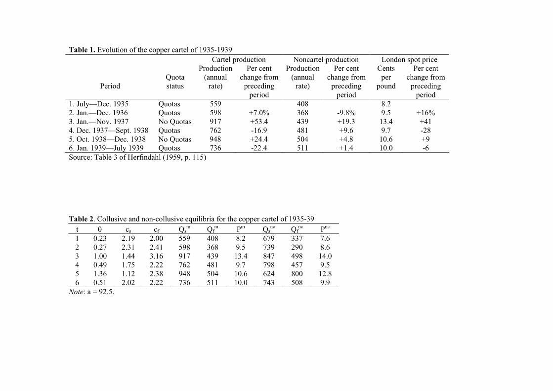
Table 1. Evolution of the copper cartel of 1935-1939 Cartel production Noncartel production London spot price
Period
Quota status
Production (annual
rate)
Per cent change from
preceding period
Production (annual
rate)
Per cent change from
preceding period
Cents per
pound
Per cent change from
preceding period
1. July—Dec. 1935 Quotas 559 408 8.2 2. Jan.—Dec. 1936 Quotas 598 +7.0% 368 -9.8% 9.5 +16% 3. Jan.—Nov. 1937 No Quotas 917 +53.4 439 +19.3 13.4 +41 4. Dec. 1937—Sept. 1938 Quotas 762 -16.9 481 +9.6 9.7 -28 5. Oct. 1938—Dec. 1938 No Quotas 948 +24.4 504 +4.8 10.6 +9 6. Jan. 1939—July 1939 Quotas 736 -22.4 511 +1.4 10.0 -6 Source: Table 3 of Herfindahl (1959, p. 115) Table 2. Collusive and non-collusive equilibria for the copper cartel of 1935-39
t θ cs cf Qsm Qf
m Pm Qsnc Qf
nc Pnc 1 0.23 2.19 2.00 559 408 8.2 679 337 7.6 2 0.27 2.31 2.41 598 368 9.5 739 290 8.6 3 1.00 1.44 3.16 917 439 13.4 847 498 14.0 4 0.49 1.75 2.22 762 481 9.7 798 457 9.5 5 1.36 1.12 2.38 948 504 10.6 624 800 12.8 6 0.51 2.02 2.22 736 511 10.0 743 508 9.9
Note: a = 92.5.
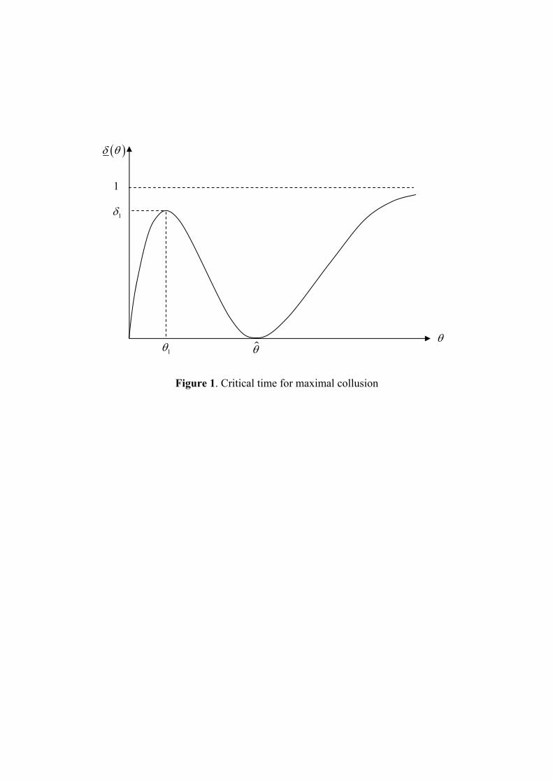
Figure 1. Critical time for maximal collusion
θ $θ
1δ
1
1θ
( )δ θ