Output - Derived Variables

• Derived Variables are quantities evaluated from the primitive (or solved) variables by PHOENICS.• It means, PHOENICS first solve U1, V1, W1, P1, TEM1 etc. After achieving convergence it evaluates the Derived Variables.• Usually they are:

Heat Transfer CoefficientsFriction Factors Shear Stresses at walls Wall Distances, etc

• Placing the Skin friction coefficient, Stanton Number, Shear stress (actually friction velocity squared, equivalent to shear stress divided by density), Yplus (non-dimensional distance to the wall) and heat transfer coefficient (in W/m2/K) into 3-D storage allows them to be plotted in the Viewer or PHOTON, as well as appearing in the RESULT file.

2

w

+

wf 21

ref2

L

p ref

''w ref

Wall Shear Stress u *

Yplus=distance from the wall y yu *

Skin Friction Coef CU

hNuStanton Number St

Re Pr C U

Local Heat Transf COeff q h T T kdT / dn

•The major difficult to establish these variables in a general purpose code lies on the determination of the reference velocity and temperature.

Output - Derived Variables – Usual Definitions

Output - Derived VariablesPHOENICS DEFINITIONS

• The phoenics uses as a reference velocity the wall velocity, i.e. , the velocity evaluated at the volume adjacent to the wall, here defined sUw

w2W

2W

w

w 1

w

p w w p w

Skin Friction Coef = SKIN=U

Shear Stress = SHEAR = SKIN* U

q kHeat Transf COeff = HTCO =

T T

q HTCOStanton Number = STAN=

C U T C U

Uw

T1

d

parede

V.C. adjacent to the wall

Output - Derived Variables

• Note that the friction and heat-transfer coefficients are only calculated for turbulent flow. To make them appear for laminar cases, the turbulent viscosity should be set to a very small value – say 1.0E-10.• •The Stanton Number must be stored for the heat-transfer coefficients to be calculated.

Output - Derived Variables

• The friction force components SHRX, SHRY and SHRZ are used in the force-integration routines to add the friction force to the pressure force acting on each object. If they are not stored, the integrated force will only contain the pressure component.

•The Total or Stagnation Pressure (PTOT) is only calculated if the Mach Number is stored. If the Reference Pressure (Main Menu – Properties) is set to zero, the total pressure may go below zero, leading to an error-stop.

Workshop #1 Friction factor and heat transfer coefficient for a laminar flow inside a circular section pipe.

• Pipe radius = 0.005 m, Pipe lenght = 1 m• Inlet velocity and temperature = 0.1 m/s and 100oC• Wall velocity and temperature = 0 m/s and 0oC

• Grid size: ny = 20 & nz = 60 (power 1.2)• Model : turbulent with constant T of 1e-10

• Set Properties Manually to:• RHO = 1; ENUL = 10-5; CP = 1000 & K = 0.02

• If every thing went wrong: Upload Q1

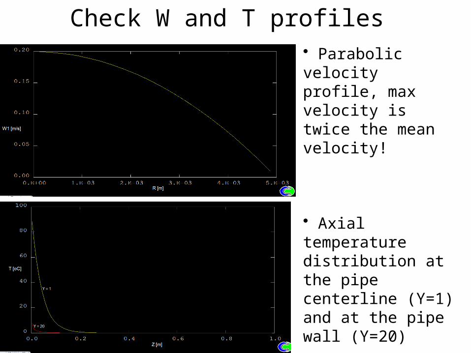
Check W and T profiles

• Parabolic velocity profile, max velocity is twice the mean velocity!

• Axial temperature distribution at the pipe centerline (Y=1) and at the pipe wall (Y=20)

Skin friction

• Shear stress evaluation at the fully developed region:

• Please, compare to the analytical solution, Cf = 16/Re

2 4W WSKIN W 8 10

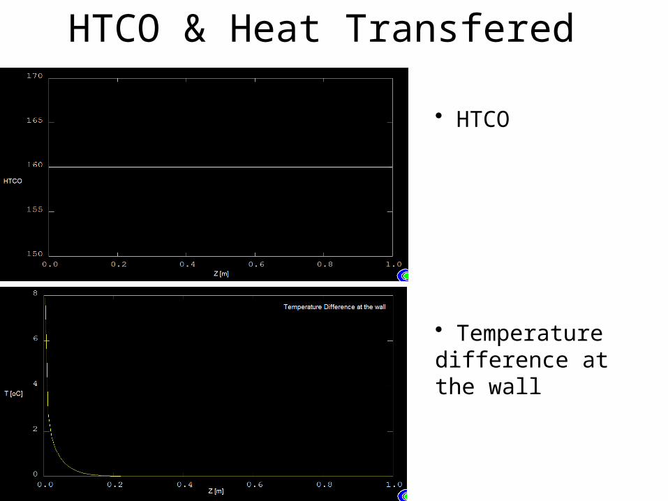
HTCO & Heat Transfered

• HTCO

• Temperature difference at the wall

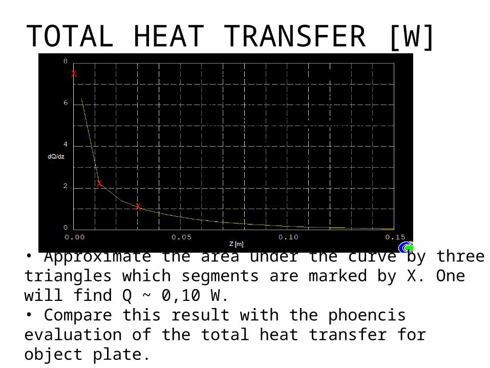
TOTAL HEAT TRANSFER [W]

Y 20 W

1

0

q HTCO T T

Q q A q R Z

dQ 160 T 0.5 0.01 dz

Q 0.80 T dz

• Approximate the area under the curve by three triangles which segments are marked by X. One will find Q ~ 0,10 W.• Compare this result with the phoencis evaluation of the total heat transfer for object plate.

Forces & Momentum in Objetcs

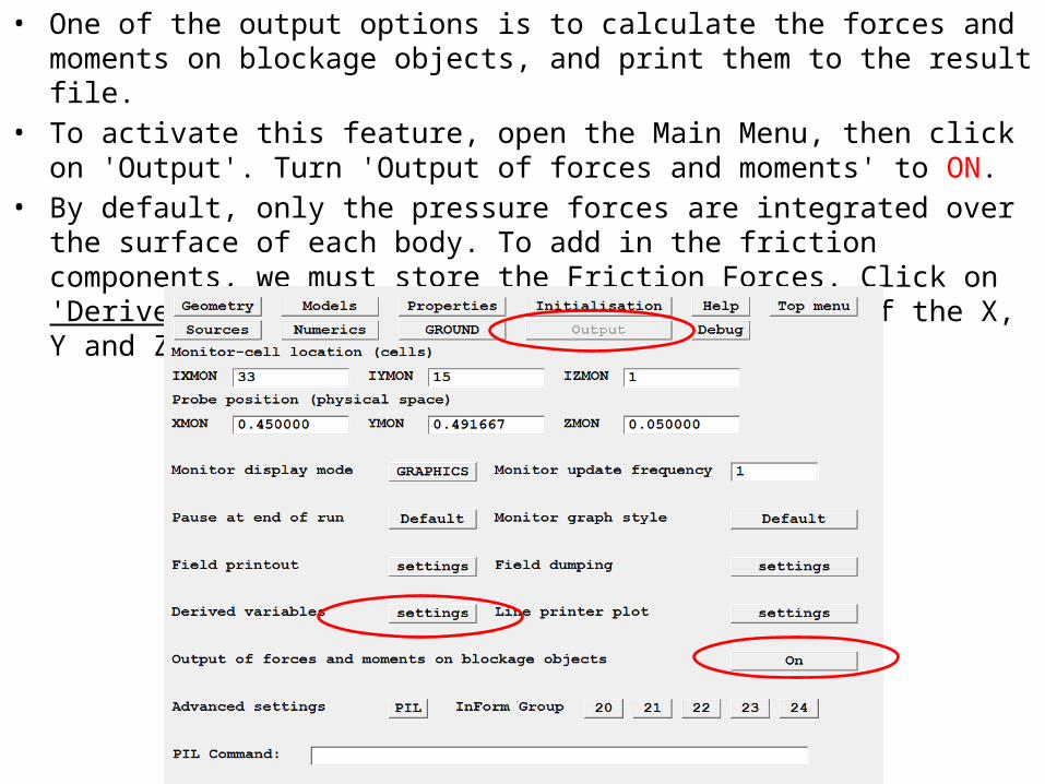
• One of the output options is to calculate the forces and moments on blockage objects, and print them to the result file.

• To activate this feature, open the Main Menu, then click on 'Output'. Turn 'Output of forces and moments' to ON.

• By default, only the pressure forces are integrated over the surface of each body. To add in the friction components, we must store the Friction Forces. Click on 'Derived variables' and turn ON the 3D storage of the X, Y and Z friction force components.

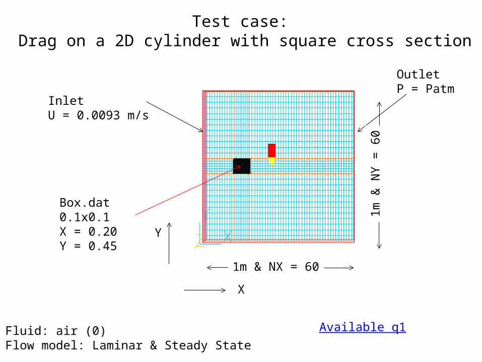
Test case: Drag on a 2D cylinder with square cross section

Y

InletU = 0.0093 m/s

OutletP = Patm

1m & NX = 60

X

1m &

NY

= 60

Box.dat0.1x0.1X = 0.20Y = 0.45

Fluid: air (0) Flow model: Laminar & Steady State

Available q1

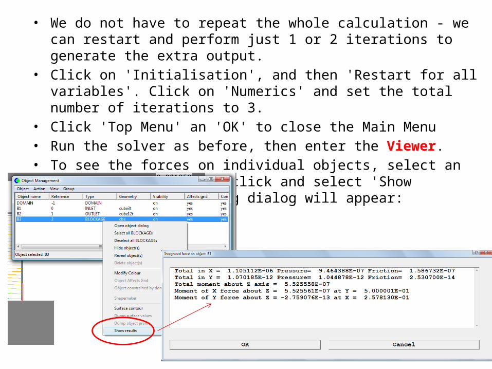
• We do not have to repeat the whole calculation - we can restart and perform just 1 or 2 iterations to generate the extra output.

• Click on 'Initialisation', and then 'Restart for all variables'. Click on 'Numerics' and set the total number of iterations to 3.

• Click 'Top Menu' an 'OK' to close the Main Menu• Run the solver as before, then enter the Viewer.• To see the forces on individual objects, select an object, say B3, right click and

select 'Show results'. The following dialog will appear:

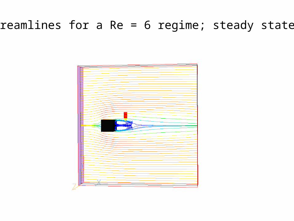
Streamlines for a Re = 6 regime; steady state flow