ECONOMIC RESEARCH CENTER

DISCUSSION PAPER

E-Series

August 2017

ECONOMIC RESEARCH CENTER

GRADUATE SCHOOL OF ECONOMICS

NAGOYA UNIVERSITY

No.E17-5

Output and Welfare Implications of

Oligopolistic Third-Degree Price

Discrimination

by

Takanori Adachi

Michal Fabinger

Output and Welfare Implications of OligopolisticThird-Degree Price Discrimination∗

Takanori Adachi† Michal Fabinger‡

July 31, 2017

Abstract

Using estimable concepts, we provide sufficient conditions for price dis-crimination to lower or raise aggregate output and social welfare under sym-metrically differentiated oligopoly with general demand functions and costdifferences across separated markets. Assuming that all markets are open un-der uniform pricing, we show that if the markup ratio in the strong market(where the discriminatory price is higher than the uniform price) relative tothe weak market (where it is lower) is sufficiently large under uniform pricing,then social welfare will be lower if price discrimination is allowed. It is alsoshown that if either the conduct ratio, the pass-through ratio, or the markupratio is sufficiently small in the strong market under price discrimination, thenit raises social welfare.

Keywords: Third-Degree Price Discrimination; Differentiated Oligopoly; So-cial Welfare; Pass-through.

JEL classification: D21; D43; D60; L11; L13.

∗We are grateful to Nicolas Schutz for helpful comments. Adachi acknowledges a Grant-in-Aid for Scientific Research (C) (15K03425) from the Japan Society of the Promotion of Science.Fabinger acknowledges a Grant-in-Aid for Young Scientists (A) (26705003) from the Society. Allremaining errors are our own.†School of Economics, Nagoya University, 1 Furo-cho, Chikusa-ku, Nagoya 464-8601, Japan.

E-mail: adachi.t@soec.nagoya-u.ac.jp‡Graduate School of Economics, University of Tokyo, 7-3-1 Hongo, Bunkyo-ku, Tokyo 113-

0033, Japan. Fabinger is also a research associate at CERGE-EI, Prague, Czech Republic. E-mail:fabinger@e.u-tokyo.ac.jp.

1

1 Introduction

In this paper, we extend Aguirre, Cowan, and Vickers’ (2010) arguments of the

welfare effects of monopolistic third-degree price discrimination to the case of (sym-

metric) oligopoly. In particular, we emphasize the role of pass-through as in Weyl

and Fabinger (2013) and Adachi and Fabinger (2017). Furthermore, we allow cost

differentials across discriminatory markets as in Chen and Schwartz (2015). Assum-

ing that marginal costs are constant and that all markets are open under uniform

pricing, we show that if the markup ratio in the strong market (where the discrimi-

natory price is higher than the uniform price) relative to the weak market (where it

is lower) is sufficiently large under uniform pricing, then social welfare will be lower

if price discrimination is allowed. It is also shown that if either the conduct ratio,

the pass-through ratio or the markup ratio is sufficiently small in the strong market

under price discrimination, then it raises social welfare.

In almost all of the theoretical studies on price discrimination, researchers (man-

ually) assume that there are no cost differentials across discriminatory markets to

focus on the demand side. However, in many real-world cases of price discrimina-

tion, cost differentials are quite often observed, not to mention the typical example

of a first-class seat and an economy-class seat (see Phlips 1983, pp. 5-7). In the nar-

row definition of price discrimination, this is not price discrimination because they

are considered different products. However, airlines are arguably motivated to offer

different types of seats because they aim to exploit consumer surplus by making

use of heterogeneity among consumers. Thus, ideally, a theoretical analysis of price

discrimination should also allow cost differentials across discriminatory markets.

Even if costs differ across markets, sellers, in reality, may have to be engaged

in uniform pricing due to the universal service requirement, fairness concerns from

consumers, and so on. Following Robinson (1933), we call one market s (strong),

where the equilibrium discriminatory price, ps, will be higher, if price discrimination

is allowed, than the equilibrium uniform price, p, and the other w (weak), where the

opposite is true, and the equilibrium discriminatory price is denoted by pw.1 In the

1In this paper, price discrimination is present when ps > pw. As Clerides (2004, p. 402) argues,

2

case of monopoly with constant marginal costs, Chen and Schwartz (2015) derive

sufficient conditions for consumer surplus to be higher under differential pricing. To

ensure that the strong market is indeed strong when cost differentials are allowed,

it is sufficient to assume that the marginal cost in the strong market is higher than

in the weak market: cs > cw (though cs should not be too much higher than cw).

Then, under uniform pricing, the markup in the strong market p−cs is smaller than

the markup in the weak market p − cw. Differential pricing allows the monopolist

to sell more products in the weak market which is more efficient than the other

market. Chen and Schwartz (2015) find that while differential pricing with no cost

differentials (third-degree price discrimination in a traditional manner) tends to

increase the average price after differential pricing is allowed, differential pricing

with cost differentials does not. As in Chen and Schwartz (2015), this paper does

not have to make an explicit assumption on cs and cw as long as the second-order

conditions are satisfied and a large discrepancy between cw and cw does not change

the order of the discriminatory prices from the one with no cost differentials.2

We also emphasize that our sufficient conditions are related to estimable con-

cepts. Interestingly, own- and cross-price elasticities per se do not play an important

role in welfare evaluation. Our theoretical predictions, equipped with an estimable

framework, would be utilized to understand the mechanism behind an empirical

result. For example, in their empirical analysis of within-store brand competition,

Hendel and Nevo (2013) show that social welfare is higher under third-degree price

discrimination than with the case with no discrimination. However, it is not clear

what mechanism makes this empirical result. Although welfare evaluation is ulti-

mately an empirical matter, one still wishes to know more about which force derives

once cost differentials are allowed, “there is no single, widely accepted definition of price discrim-ination.” To understand this issue, let mcs and mcw be equilibrium marginal costs in markets sand w, respectively. Then, there are two alternative definitions. One is the margin definition:price discrimination occurs when ps −mcs > pw −mcw. The other one is the markup definition:price discrimination occurs when ps/mcs > pw/mcw. In this paper, we employ the simplest defi-nition. As long as cost differentials are sufficiently small, these differences will not alter the resultssignificantly because these three definitions are equivalent if mcs = mcw.

2In the context of reduced-fare parking as a form of third-degree price discrimination, Floresand Kalashnikov (2017) characterize a sufficient condition for free parking (drivers receive a pricediscount in the form of complentary parking while pedestrians do not) to be welfare improving.

3

the result. Thus, this paper also aims to fill the gap between theoretical predictions

and the empirical literature of price discrimination, where researchers often have to

remain agnostic about the mechanism behind the result.

The rest of the paper is organized as follows. Section 2 presents our basic model

with symmetric firms and constant marginal costs. Then, we derive output and

welfare implications in Section 3. Section 4 concludes the paper.

2 Symmetric Firms with Constant Marginal Costs

For ease of exposition, we, following Holmes (1989) and Aguirre, Cowan, and Vickers

(2010), consider the case of two symmetric firms and two separate markets or con-

sumer groups (simply called markets hereafter). Extending the following analysis

to the case of J (≥ 3) symmetric firms and M (≥ 3) separate markets is straight-

forward. As explained above, we call one market s (strong), where the equilibrium

discriminatory price will be higher than the equilibrium uniform price, and the other

w (weak), where the opposite is true. Two firms, A and B, have an identical cost

structure in each market. We assume that they have a constant marginal cost in

each market m, cm ≥ 0. In the spirit of Chen and Schwartz (2015), cs and cw can

be different.

In market m = s, w, given firms A and B’s prices pA,m and pB,m, the represen-

tative consumer consumes qA,m > 0 and qB,m > 0, and her (net) utility is written

as Um(qA,m, qB,m) − pA,mqA,m − pB,mqB,m, where Um is twice continuously differen-

tiable, ∂Um/∂qjm > 0, ∂2Um/∂q2jm > 0, j = A, B, and ∂2Um/(∂qA,m∂qB,m) < 0.

The direct demands in market m are derived from the representative consumer’s

utility maximization: ∂Um(qjm, q−j,m)/∂qjm − pjm = 0, which leads to firm j’s

demand in market m, qjm = xjm(pjm, p−j,m). We assume that xjm is twice con-

tinuously differentiable. The corresponding inverse demand can be written as

pjm = pjm(qjm, q−j,m). Because of the assumptions on the utility, firm j’s demand in

market m falls as its own price increases (∂xjm/∂qjm < 0), and it rises as the rival’s

price increases (∂xjm/∂q−j,m > 0; the firms’ products are substitutes). We assume

4

that for a consumer’s perspective firms are symmetric: Um(q′, q′′) = Um(q′′, q′) for

any q′ > 0 and q′′ > 0. Then, the firms’ demands in market m are also symmetric:

xA,m(p′, p′′) = xB,m(p′′, p′) for any p′ > 0 and p′′ > 0. Because the firms’ technologies

are also identical, we, throughout this paper, focus on symmetric Nash equilibrium.

Under the regime of uniform pricing, the equilibrium uniform price for both markets

is p. If price discrimination is allowed, the equilibrium discriminatory prices are p∗s

in the strong market and p∗w in the weak market, and functional and parametric

restrictions are imposed to assure that p∗s > p > p∗w.3

We define the demand in symmetric pricing by qm(p) ≡ xA,m(p, p). Another in-

terpretation of qm(p) is: both firms take 2qm(p) as the joint demand, ‘cooperatively’

choose the same price (behaving as an ‘industry’), and divide the joint demand

equally to obtain qm(p). Note that:

q′m(p) =∂xA,m∂pA

(pA, p)

∣∣∣∣pA=p︸ ︷︷ ︸

<0

+∂xA,m∂pB

(p, pB)

∣∣∣∣pB=p︸ ︷︷ ︸

>0 if substitutes

.

Thus, for q′m(p) to be negative, we assume that |∂xA,m(p, p)/∂pA| > ∂xA,m(p, p)/∂pB.

Note also that by symmetry the following relationship also holds:

∂xA,m∂pA

(p, p)︸ ︷︷ ︸own

= q′m(p)︸ ︷︷ ︸industry

− ∂xB,m∂pA

(p, p)︸ ︷︷ ︸strategic effects

,

which corresponds to Holmes’ (1989) equation (4). This exchangeability is to key

in Holmes’ (1989) derivation below. Intuitively, under symmetry, each firm treats

the industry demand qm(p) as if it is its own demand. Thus, how a firm’s pricing

behavior affects its own demand as an industry demand has the following two effects:

a small decrease in pA by firm A by deviating from the ‘coordinated’ price p (i) not

only raises its own demand by ∂xA,m/∂pA as the residual monopolist (taking the

rival’s pricing as fixed; intrinsic effects), (ii) firm A can now also obtain some of the

3However, see Nahata, Ostaszewski, and Sahoo (1990) for an example of all discriminatoryprices being lower than the uniform price with a plausible demand structure under monopoly. Inthe case of oligopoly, Corts (1998) show that best-response asymmetry, by which firms differ inranking strong and weak markets, is necessary to all discriminatory prices to be lower than theuniform price (“all-out price competition”).

5

consumers originally attached to firm B, and this amount is ∂xB,m/∂pA (strategic

effects).

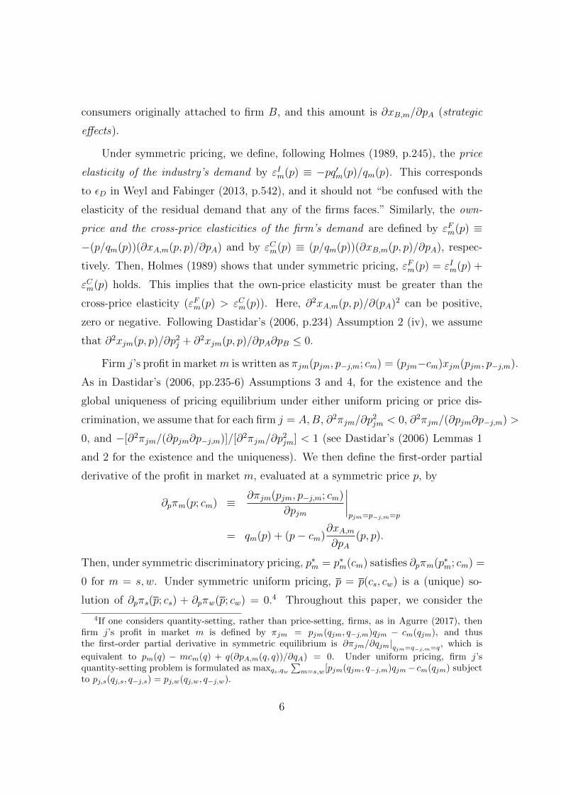
Under symmetric pricing, we define, following Holmes (1989, p.245), the price

elasticity of the industry’s demand by εIm(p) ≡ −pq′m(p)/qm(p). This corresponds

to εD in Weyl and Fabinger (2013, p.542), and it should not “be confused with the

elasticity of the residual demand that any of the firms faces.” Similarly, the own-

price and the cross-price elasticities of the firm’s demand are defined by εFm(p) ≡−(p/qm(p))(∂xA,m(p, p)/∂pA) and by εCm(p) ≡ (p/qm(p))(∂xB,m(p, p)/∂pA), respec-

tively. Then, Holmes (1989) shows that under symmetric pricing, εFm(p) = εIm(p) +

εCm(p) holds. This implies that the own-price elasticity must be greater than the

cross-price elasticity (εFm(p) > εCm(p)). Here, ∂2xA,m(p, p)/∂(pA)2 can be positive,

zero or negative. Following Dastidar’s (2006, p.234) Assumption 2 (iv), we assume

that ∂2xjm(p, p)/∂p2j + ∂2xjm(p, p)/∂pA∂pB ≤ 0.

Firm j’s profit in marketm is written as πjm(pjm, p−j,m; cm) = (pjm−cm)xjm(pjm, p−j,m).

As in Dastidar’s (2006, pp.235-6) Assumptions 3 and 4, for the existence and the

global uniqueness of pricing equilibrium under either uniform pricing or price dis-

crimination, we assume that for each firm j = A,B, ∂2πjm/∂p2jm < 0, ∂2πjm/(∂pjm∂p−j,m) >

0, and −[∂2πjm/(∂pjm∂p−j,m)]/[∂2πjm/∂p2jm] < 1 (see Dastidar’s (2006) Lemmas 1

and 2 for the existence and the uniqueness). We then define the first-order partial

derivative of the profit in market m, evaluated at a symmetric price p, by

∂pπm(p; cm) ≡ ∂πjm(pjm, p−j,m; cm)

∂pjm

∣∣∣∣pjm=p−j,m=p

= qm(p) + (p− cm)∂xA,m∂pA

(p, p).

Then, under symmetric discriminatory pricing, p∗m = p∗m(cm) satisfies ∂pπm(p∗m; cm) =

0 for m = s, w. Under symmetric uniform pricing, p = p(cs, cw) is a (unique) so-

lution of ∂pπs(p; cs) + ∂pπw(p; cw) = 0.4 Throughout this paper, we consider the

4If one considers quantity-setting, rather than price-setting, firms, as in Agurre (2017), thenfirm j’s profit in market m is defined by πjm = pjm(qjm, q−j,m)qjm − cm(qjm), and thusthe first-order partial derivative in symmetric equilibrium is ∂πjm/∂qjm|qjm=q−j,m=q, which is

equivalent to pm(q) − mcm(q) + q(∂pA,m(q, q))/∂qA) = 0. Under uniform pricing, firm j’squantity-setting problem is formulated as maxqs,qw

∑m=s,w[pjm(qjm, q−j,m)qjm− cm(qjm) subject

to pj,s(qj,s, q−j,s) = pj,w(qj,w, q−j,w).

6

situation where the weak market is open under uniform pricing: qw(p) > 0.5

Let the equilibrium profit in market m in symmetric equilibrium under uniform

pricing and under price discrimination be denoted by π∗m and πm, respectively. Ac-

cordingly, the aggregate profits are defined by Π∗ ≡ π∗s + π∗w and Π ≡ πs + πw,

respectively. If price discrimination lowers firms’ profit in symmetric pricing equi-

librium (i.e., Π∗ < Π), the firms may want to agree not to price discriminate even if

they are allowed to do so. This is a situation of Prisoners’ Dilemma: one firm’s de-

viation is profitable.6 We assume that firms cannot commit to not engaging in price

discrimination even if Π > Π∗: we consider Nash equilibrium under each regime of

pricing (uniform pricing or price discrimination).

The equilibrium discriminatory price in market m = s, w, p∗m ≡ p∗m(cm), satis-

fies the following Lerner formula: εFm(p∗m)(p∗m − cm)/p∗m = 1. This shows that the

discriminatory price in market m approaches to the marginal cost as the own-price

elasticity for the firm, εFm(p∗m), becomes large. Because of Holmes’ (1989) elasticity

formula explained above, εFm(p∗m) can be large (i) when εIm(p∗m) is very large even

if εCm(p∗m) is close to zero, or (ii) when εCm(p∗m) is very large even if εIm(p∗m) is close

to zero. These are two polar cases of a large εFm(p∗m): of course if both εIm(p∗m) and

εCm(p∗m) are very large, then εFm(p∗m) is also very large. Case (i) is where the industry

is under strong pressure from other substitutable industries7 so that a small price

increase in symmetric pricing causes a large number of consumers switching to pur-

chasing a product in other industries instead, although any consumers are very loyal

to either firm so that a small price increase by one firm causes a very small number

5Note that qw(p) > qw(p∗s) because qw(·) is strictly decreasing and p∗s > p. By Assumption,qw(p∗s) > 0. Thus, the weak market is open under uniform pricing, i.e., qw(p) > 0. Alternatively,we would be able to show that there exist cs and cs, cs < cs, such that p∗s > p∗w and qw(p) > 0 forcs ∈ (cs, cs) in a similar spirit of Adachi and Matsushima (2014).

6Dastidar (2006) provides a sufficient condition for firms’ equilibrium profit to be higher underprice discrimination. More specifically, define the price difference between the discriminatory priceand the uniform price in market m by ∆p∗m ≡ p∗m − p. Then, Dastidar’s Proposition 2 (2006,p. 241) shows that if |∆p∗s| ≥ |∆p∗w| and ∂xB,s(p, p)/∂pA ≥ ∂xB,w(p, p)/∂pA for all p ∈ (p∗w, p

∗s),

then the per-firm profit difference, ∆Π ≡ Π∗ −Π, is positive.7In the demand construction based on random utility and discrete choice, this would be inter-

preted as an outside option. Note also that if the industry is defined by the SSNIP (“Small butSignificant and Non-transitory Increase in Price”) test, then by definition, εIm(p∗m) is close to zero,and thus, εFm(p∗m) is closely approximated by εCm(p∗m).

7

of consumers switching to other rivals’ product in the same industry (most of them

leave the industry to purchase something outside the industry). For example, in a

residential area, consumers (especially young consumers) would have a strong taste

for their favorite soda (thus, εCm(p∗m) is close to zero), although soda is highly sub-

stitutable by mineral water (thus, εIm(p∗m) is very large) if consumers just want to

quench their thirst (whether soda or water does not matter).

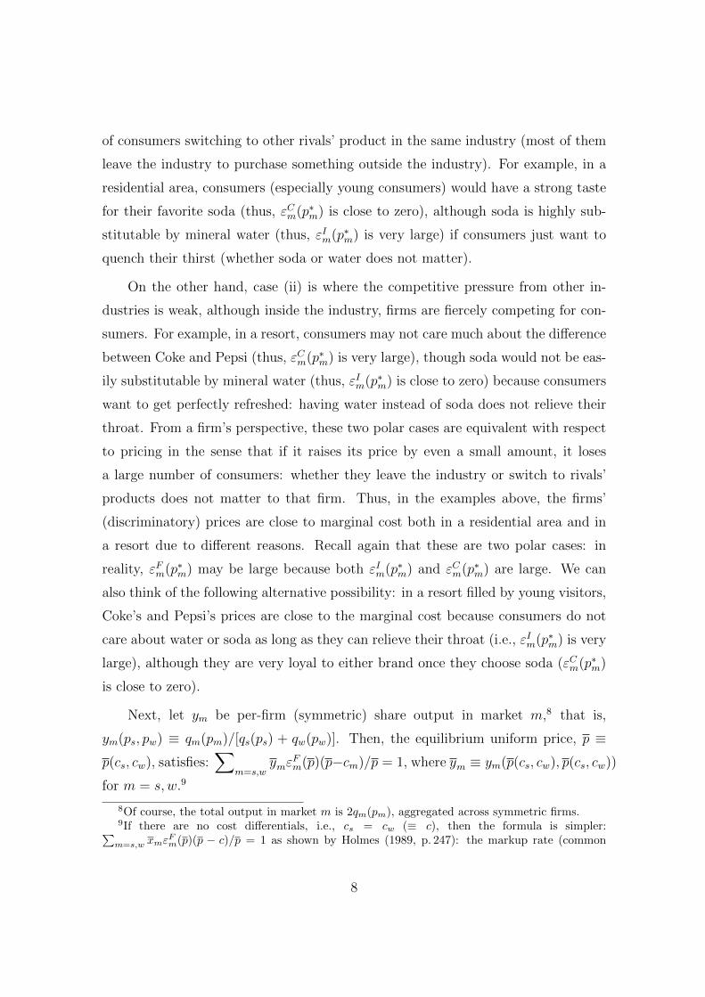
On the other hand, case (ii) is where the competitive pressure from other in-

dustries is weak, although inside the industry, firms are fiercely competing for con-

sumers. For example, in a resort, consumers may not care much about the difference

between Coke and Pepsi (thus, εCm(p∗m) is very large), though soda would not be eas-

ily substitutable by mineral water (thus, εIm(p∗m) is close to zero) because consumers

want to get perfectly refreshed: having water instead of soda does not relieve their

throat. From a firm’s perspective, these two polar cases are equivalent with respect

to pricing in the sense that if it raises its price by even a small amount, it loses

a large number of consumers: whether they leave the industry or switch to rivals’

products does not matter to that firm. Thus, in the examples above, the firms’

(discriminatory) prices are close to marginal cost both in a residential area and in

a resort due to different reasons. Recall again that these are two polar cases: in

reality, εFm(p∗m) may be large because both εIm(p∗m) and εCm(p∗m) are large. We can

also think of the following alternative possibility: in a resort filled by young visitors,

Coke’s and Pepsi’s prices are close to the marginal cost because consumers do not

care about water or soda as long as they can relieve their throat (i.e., εIm(p∗m) is very

large), although they are very loyal to either brand once they choose soda (εCm(p∗m)

is close to zero).

Next, let ym be per-firm (symmetric) share output in market m,8 that is,

ym(ps, pw) ≡ qm(pm)/[qs(ps) + qw(pw)]. Then, the equilibrium uniform price, p ≡p(cs, cw), satisfies:

∑m=s,w

ymεFm(p)(p−cm)/p = 1, where ym ≡ ym(p(cs, cw), p(cs, cw))

for m = s, w.9

8Of course, the total output in market m is 2qm(pm), aggregated across symmetric firms.9If there are no cost differentials, i.e., cs = cw (≡ c), then the formula is simpler:∑m=s,w xmε

Fm(p)(p − c)/p = 1 as shown by Holmes (1989, p. 247): the markup rate (common

8

3 Output and Welfare

In the analysis below, we, following Schmalensee (1981), Holmes (1989), and Aguirre,

Cowan, and Vickers (2010), add the constraint ps−pw ≤ r, where r > 0, to the firms’

profit maximization problem (under symmetric pricing). Then, r = 0 corresponds

to uniform pricing, and r = r∗ ≡ p∗s − p∗w to price discrimination. We express social

welfare (and aggregate output) as a function of r in [0, r∗]. Note that under this

constrained problem of profit maximization, pw satisfies ∂pπs(pw+r)+∂pπw(pw) = 0.

Thus, we write the solution by pw(r). Then, we define ps(r) ≡ pw(r) + r. Applying

the implicit function theorem to this equation yields to p′w(r) = −π′′s/(π′′s + π

′′w) < 0

and p′s(r) = π′′w/(π

′′s + π

′′w) > 0.

Here, note that π′′m(p, cm) and ∂2

pπm(p, cm) are different:

π′′

m(p, cm) = q′m(p) +∂xA,m∂pA

(p, p) + (p− cm)d

dp

(∂xA,m∂pA

(p, p)

)= ∂2

pπm(p) +∂xA,m∂pB

(p, p) + (p− cm)∂2xA,m∂pB∂pA

(p, p),

where ∂2pπm(p, cm) is defined by

∂2pπm(p) ≡

[2 + (p− cm)

∂2xA,m(p, p)/∂p2A

∂xA,m(p, p)/∂pA

]∂xA,m∂pA

(p, p),

which corresponds to Aguirre, Cowan, and Vickers’ (2010) π′′m(p). We assume that

π′′m(p, cm) < 0 for all p ≥ 0.10

We define the representative consumer’s utility in symmetric pricing by Um(q) =

Um(q, q). Aggregate output under symmetric pricing is given by Q(r) = Qs(r) +

Qw(r) = 2 (qs(ps(r)) + qw(pw(r)). Social welfare under symmetric pricing as a func-

tion of r is written as W (r; cs, cw) ≡ Us(qs(ps(r))) + Uw(qw(pw(r)))−2cs · qs(ps(r))−2cw · qw(pw(r)), which implies W ′(r) ≡ (U ′s− 2cs) · q′s · p′s(r) + (U ′w − 2cw) · q′w · p′w(r).

Now, note that U ′m = ∂Um/∂qA + ∂Um/∂qB = 2∂Um/∂qA (by symmetry). Thus,

W ′(r) = 2 (ps(r)− cs) · q′s · p′s(r) + 2 (pw(r)− cw) · q′w · p′w(r).

to all markets) is equal to the inverse of the average of own-price elasticities weighted by theoutput shares.

10Appendix A of Aguirre, Cowan, and Vickers (2010) discusses the concavity of the profit func-tion.

9

3.1 Output

Now, we can further proceed:

W ′(r)

2= (ps(r)− p+ p− cs) q′s(ps(r))p′s(r)

+ (pw(r)− p+ p− cw) q′w(pw(r))p′w(r)

= (ps(r)− p) q′s(ps(r))p′s(r)︸ ︷︷ ︸<0

+ (pw(r)− p) q′w(pw(r))p′w(r)︸ ︷︷ ︸<0

+∑m=s,w

(p− cm) q′m(pm(r))p′m(r).

This derivation coincides with the case of monopoly as shown in Aguirre, Cowan, and

Vickers’ (2010, p. 1604) equality (3) if there are no cost differentials (i.e., cs = cw ≡c), with two minor modifications: (i) the left hand side is W ′(r)/2 rather than W ′(r)

itself, and (ii) the last term of Aguirre, Cowan, and Vickers’ (2010) equality (3) is re-

placed byQ′(r)/2 rather thanQ′(r) because (1/2)∑

m=s,w (p− cm) q′m(pm(r))p′m(r) =

(p− c) (Q′(r)/2). If cost differentials are allowed, it is observed that an increase in

the weighted aggregate output,∑

m=s,w (p− cm) q′m(pm(r))p′m(r), is necessary for

price discrimination to raise social welfare, as in the case of monopoly.11

To proceed further, we define the curvature of the firm’s (direct) demand in

market m by

αFm(p) ≡ − p

∂xA,m(p, p)/∂pA

∂2xA,m∂p2

A

(p, p)

(which measures the concavity/convexity of the firm’s direct demand, and corre-

sponds to αm(p) in Aguirre, Cowan, and Vickers, 2010, p. 1603), and the elasticity

of the cross-price effect of the firm’s direct demand in market m by

αCm(p) ≡ − p

∂xA,m(p, p)/∂pB

∂2xA,m∂pB∂pA

(p, p)

= − p

∂xB,m(p, p)/∂pA︸ ︷︷ ︸>0

∂2xB,m∂p2

A

(p, p)︸ ︷︷ ︸<0

,

11However, if externalities across consumers, such as network externalities and congestion, exist,then an increase in aggregate output would be no longer a necessary condition, as implied byAdachi (2002, 2005), who studies monopoly with linear demands. See also Czerny and Zhang(2015) as a recent study of price discrimination and congestion.

10

which is new to oligopoly.12 Here, αFm(p) is positive (resp. negative) if and only if

∂2xA,m(p, p)/∂p2A is negative (resp. positive), while αCm(p) is always positive (because

of our assumption, ∂2xjm(p, p)/(∂pA∂pB) < 0). Note that the sign of αFm(p) indicates

whether the firm’s own part of the demand slope under symmetric pricing given the

rival’s price being p, ∂xA,m(·, p)/∂pA, is convex (αFm(p) is positive) or concave (αFm(p)

is negative). On the other hand, αCm(p) measures how the rival’s price level matters

to how many of the firm’s customers switch to the rival’s product when the firm

raises its own price (∂xB,m/∂pA). Thus, a large αCm(p) implies that ∂xB,m/∂pA is

very responsive to a change in pB, and vice versa.

Next, we define the conduct index (see, e.g., Bresnahan 1989; Genesove and

Mullin 1998; and Corts 1999) in market m by θm(p) ≡ 1 − Am(p),13 where Am(p)

is the aggregate diversion ratio (Shapiro 1996) in market m, which is is defined

by Am(p) ≡ −(∂xB,m(p, p)/∂pA)/(∂xA,m(p, p)/∂pA) = εCm(p)/εFm(p). Here, Am(p)

measures the degree of rivalness : if Am(p) is close to one, consumers who leave a

firm as a response to an increase in its price are nearly all switching to its rival’s

product. In this way, Aguirre, Cowan, and Vickers’ (2010) derivation in the case

of monopoly (where the method by Schmalensee (1981) is utilized) is connected

to Weyl and Fabinger’s (2013) condition in the case of symmetric oligopoly. In

particular, Aguirre, Cowan, and Vickers’ (2010, p.1606) Proposition 2 (a sufficient

condition for price discrimination to raise social welfare) is extended to the case of

12This is because ∂ (∂xA,m(p, p)/∂pB) /∂pA = ∂ (∂xB,m(p, p)/∂pA) /∂pA.13Alternatively, Weyl and Fabinger (2013, p. 531) define the conduct index in a market (which,

in our interest in price discrimination, can be indexed by m) by θm ≡ [(p − cm)/p]εIm (their mcand εD are replaced by our cm and εIm, respectively) as the Lerner index adjusted by the elasticityof the industry’s demand. If the first-order condition is given for each market (that is, if fullprice discrimination is allowed), then θm(p) defined as in Weyl and Fabinger (2013) coincides with1−Am(p) because εFm[(pm − cm)/pm] = 1 and thus

εIm(p)p− cmp

=1

εFm(p)

(− p

qm(p)

)q′m(p)

= −qm(p)

p

1

∂xA,m(p, p)/∂pA

(− p

qm(p)

)(∂xA,m

∂pA(p, p) +

∂xA,m

∂pB(p, p)

)=

∂xA,m(p, p)/∂pA + ∂xB,m(p, p)/∂pA∂xA,m(p, p)/∂pA

(by symmetry).

See also Adachi and Fabinger (2017) for a generalized definition of the conduct index that allowsfor the possibly of non-zero specific and ad valorem taxes.

11

oligopoly in a simpler manner, using the concept of pass-through introduced in the

next subsection.

As Weyl and Fabinger (2013, p. 544) argue, θm(p) captures the degree of industry-

level brand loyalty or stickiness14 in market m: if θm(p) is zero (close to one), market

m is captured by perfect competition (almost monopoly): firms’ products are per-

fect substitutes (nearly non-substitutable products).15 The markup rate (the Lerner

index), Lm(pm, cm) ≡ (pm − cm)/pm, alone is not appropriate to measure the rival-

ness within market m because it can be the case that pm is close to cm (the markup

rate is close to zero) simply because the price elasticity of the industry’s demand

εIm(pm) is very large while the brand rivalness is so weak that the cross-price elas-

ticity, εCm(pm), remains very small (as a result, in total, εFm(pm) is very large, which

is actually reason for the low markup rate). However, if εCm(pm) is close to εFm(pm)

(i.e., almost of all consumers who leave a firm as a response to its price increase are

switching to other rivals’ products), then θm becomes close to zero irrespective of

the value of the markup rate. Thus, θm(p), which ranges between 0 and 1, better

captures the brand stickiness than Lm(p, cm) does.

Now, we consider the effects of price discrimination on aggregate output. First,

note that

Q′(r)

2= q′w · p′w + q′s · p′s

=

(− π

′′sπ′′w

π′′s + π′′w

)︸ ︷︷ ︸

>0

×(

1− Ls(ps(r))[αFs (ps(r))− (1− θs(ps(r))αCs (ps(r))]

θs(ps(r))

−1− Lw(pw(r))[αFw(pw(r))− (1− θw(pw(r))αCw(pw(r))]

θw(pw(r))

).

Note also that εCm(pm)/εIm(pm) = [1− θm(pm)]/θm(pm) measures the substitutability

14Even if the firms’ products have the same characteristics across different markets (with noproduct differentiation), the degree of brand loyalty may differ across markets, reflecting differencesin market characteristics (summarized in demand functions).

15Because (pm − cm)εFm(pm)/pm = 1 and εFm(pm) = εIm(pm) + εCm(pm), it is verified thatθm(pm, cm)+εCm(pm)(pm−cm)/pm = 1. Thus, as long as the products are substitutes (εCm(pm) > 0),θm(pm, cm) is less than one.

12

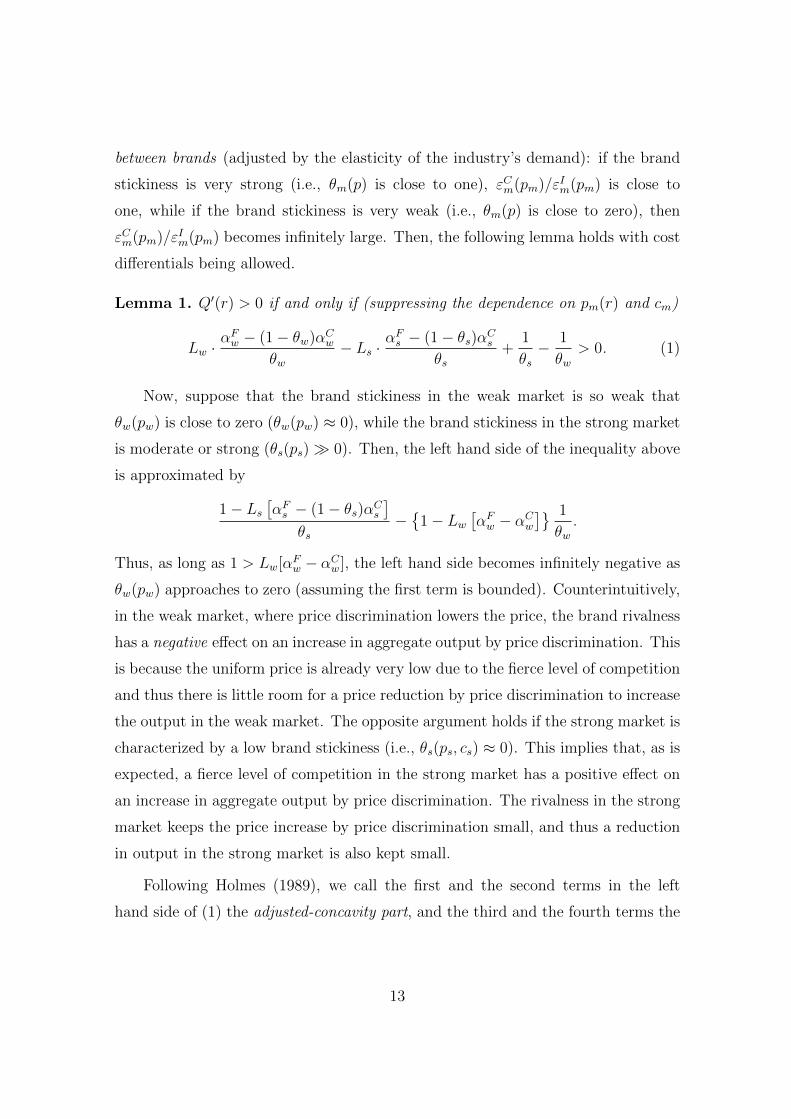
between brands (adjusted by the elasticity of the industry’s demand): if the brand

stickiness is very strong (i.e., θm(p) is close to one), εCm(pm)/εIm(pm) is close to

one, while if the brand stickiness is very weak (i.e., θm(p) is close to zero), then

εCm(pm)/εIm(pm) becomes infinitely large. Then, the following lemma holds with cost

differentials being allowed.

Lemma 1. Q′(r) > 0 if and only if (suppressing the dependence on pm(r) and cm)

Lw ·αFw − (1− θw)αCw

θw− Ls ·

αFs − (1− θs)αCsθs

+1

θs− 1

θw> 0. (1)

Now, suppose that the brand stickiness in the weak market is so weak that

θw(pw) is close to zero (θw(pw) ≈ 0), while the brand stickiness in the strong market

is moderate or strong (θs(ps)� 0). Then, the left hand side of the inequality above

is approximated by

1− Ls[αFs − (1− θs)αCs

]θs

−{

1− Lw[αFw − αCw

]} 1

θw.

Thus, as long as 1 > Lw[αFw − αCw ], the left hand side becomes infinitely negative as

θw(pw) approaches to zero (assuming the first term is bounded). Counterintuitively,

in the weak market, where price discrimination lowers the price, the brand rivalness

has a negative effect on an increase in aggregate output by price discrimination. This

is because the uniform price is already very low due to the fierce level of competition

and thus there is little room for a price reduction by price discrimination to increase

the output in the weak market. The opposite argument holds if the strong market is

characterized by a low brand stickiness (i.e., θs(ps, cs) ≈ 0). This implies that, as is

expected, a fierce level of competition in the strong market has a positive effect on

an increase in aggregate output by price discrimination. The rivalness in the strong

market keeps the price increase by price discrimination small, and thus a reduction

in output in the strong market is also kept small.

Following Holmes (1989), we call the first and the second terms in the left

hand side of (1) the adjusted-concavity part, and the third and the fourth terms the

13

elasticity-ratio part :

Lw ·αFw − (1− θw)αCw

θw− Ls ·

αFs − (1− θs)αCsθs︸ ︷︷ ︸

adjusted-concavity

+1

θs− 1

θw︸ ︷︷ ︸ .

elasticity-ratio

(1’)

First, look at the elasticity-ratio part. If the difference θw − θs is greater, it is more

likely that Q′(r) > 0. Thus, competitiveness in the strong market, rather than in the

weak market, is important. Next, look at the adjusted-concavity part. A larger αFw

and/or a smaller αCw make a positive Q′(r) more likely. A larger αFw means that the

firm’s own part of the demand in the weak market (∂xA,w/∂pA) is more convex. On

the other hand, a smaller αCw means that how many of the firm’s customers switch

to the rival’s product as response to the firm’s price increase is not so affected by

the current price level. In this sense, the strategic concerns in the firm’s pricing are

small. Thus, both a larger αFw and a smaller αCw indicate that the weak market is

competitive. Even if ∂xA,w/∂pA is not so convex, a smaller αCw (i.e., ∂xB,m/∂pA is

not responsive to the level of pB) can substitute it. A similar argument also holds

for αFs and αCs . In the Appendix, we show that Holmes’ (1989) expression for Q′(r)

(expression (9) in Holmes (1989, p. 247)) is equivalent to (1’).

Now, define hm(p, cm) ≡ 1/(q′m(p)/π′′m(p, cm)) > 0 so that

Q′(r)

2=

(− q

′sq′w

π′′s + π′′w

)︸ ︷︷ ︸

>0

[hs(ps(r), cs)− hw(pw(r), cw)] .

We assume that hm(·, cm) is decreasing (and call it the Decreasing Inverse Ratio

Condition: DIRC).16 It is also shown that

Q′′(r)

2=

(− q

′sq′w

π′′s + π′′w

)[h′sp

′s − h′wp′w] + [hs − hw]

d

dr

(− q

′sq′w

π′′s + π′′w

).

16It is verified that h′m < 0 is equivalent to q′′m > (q′m/π′′m)π′′′m because

h′m(p, cm) =

(π′′

m(p, cm)

q′m(p)

)′=π′′′mq

′m − π′′mq′′m[q′m]2

.

Thus, DIRC states that the profit function decreases quickly enough as p increases. To see this,if q′′m > 0, then it is sufficient to assume π′′′m < 0. This means that π′′m, which is negative, shouldbe smaller, that is, the the negative slope of π′′m should be steeper, as p increases. If q′′m ≤ 0, thenπ′′m be should be not only negative but sufficiently small that π′′′m < q′′m/(q

′m/π

′′m). In both cases,

πmshould decrease quickly as p increases.

14

Then, there exists r such thatQ′(r) = 0 andQ′′(r)/2 = [−q′sq

′w/(π

′′s+π

′′w)] [h′sp

′s − h′wp′w] <

0 because h′sp′s < 0 and h′wp

′w > 0. Then, (1/2)Q(r) behaves on [0, r∗] in either man-

ner:17

1. If Q′(0) ≤ 0, then (1/2)Q(r) is monotonically decreasing in r, and a result

∆Q/2 = [Q(r∗; cs, cw)−Q(0; cs, cw)]/2 < 0; price discrimination lowers aggre-

gate output.

2. If Q′(0) > 0, then (1/2)Q(r) either

(a) is monotonically increasing (if Q′(r∗) > 0, this is true), and as a result,

∆Q/2 > 0; price discrimination raises aggregate output.

(b) first increases, and then after the reaching the maximum (where Q′(r) =

0), decreases until r = r∗. In this case, price discrimination may raise or

lower aggregate output : it cannot be determined whether ∆Q/2 < 0 or

∆Q/2 > 0 without further functional and/or parametric restrictions.

Now, we determine the sign ofQ′(0). It follows that sign[Q′(0)] = sign[π′′s (p, cs)/q

′s(p)−

π′′w(p, cw)/q′w(p)], which implies that Q′(0) ≤ 0⇔ π

′′w(p, cw)/q′w(p) ≥ π

′′s (p, cs)/q

′s(p).

Note also that sign[Q′(r∗)] = sign[hs(p∗s, cs)−hw(p∗w, cw)], which implies thatQ′(r∗) >

0⇔ π′′s (p∗s, cw)/q′s(p

∗s) > π

′′w(p∗w, cw)/q′w(p∗w). Because

π′′m(p, cm)

q′m(p)=

[2− Lm(p, cm)αFm(p)

]− [1− θm(p)]

[1− Lm(p, cm)αCm(p)

]θm(p)

holds, the following proposition obtains.

Proposition 1. Given the DIRC, if θs(p) ≥ θw(p) and

αFs (p)− [1− θs(p)]αCs (p)

θs(p)≥ αFw(p)− [1− θw(p)]αCw(p)

θw(p)

then price discrimination lowers aggregate output. If θw(p∗w) > θs(p∗s) and

αFw(p∗w)− [1− θw(p∗w)]αCw(p∗w)

θw(p∗w)≥ αFs (p∗s)− [1− θs(p∗s)]αCs (p∗s)

θs(p∗s),

then price discrimination raises aggregate output.17This is because the modified version of Aguirre, Cowan, and Vickers’ (2010, p. 1605) Lemma

also holds in our oligopoly setting.

15

Proof. First, note that[2− Lw(p, cw)αFw(p)

]− [1− θw(p)]

[1− Lw(p, cw)αCw(p)

]θw(p)

≥[2− Ls(p, cs)αFs (p)

]− [1− θs(p)]

[1− Ls(p, cs)αCs (p)

]θs(p)

,

then price discrimination lowers aggregate output. The first part is a sufficient

condition for this inequality to hold. Next, note that[2− Ls(p∗s, cs)αFs (p∗s)

]− [1− θs(p∗s)]

[1− Ls(p∗s, cs)αCs (p∗s)

]θs(p∗s)

>

[2− Lw(p∗w, cw)αFw(p∗w)

]− [1− θw(p∗w)]

[1− Lw(p∗w, cw)αCw(p∗w)

]θw(p∗w)

,

then price discrimination raises aggregate output. Thus, θw(p∗w) > θs(p∗s) and

Lw(p∗w, cw)αFw(p∗w)− [1− θw(p∗w)]αCw(p∗w)

θw(p∗w)> Ls(p

∗s, cs)

αFs (p∗s)− [1− θs(p∗s)]αCs (p∗s)

θs(p∗s).

3.2 Social Welfare

Now, we study the effects of allowing third-degree price discrimination on social

welfare. To proceed further, note that

W ′(r)

2=

(− π

′′sπ′′w

π′′s + π′′w

)︸ ︷︷ ︸

>0

×(

(pw(r)− cw)q′w(pw(r))

π′′w− (ps(r)− cs)q′s(ps(r))

π′′s

).

We follow Aguirre, Cowan, and Vickers (2010, p. 1605), who define zm(p, cm) ≡(p−cm)q′m(p)/π

′′m(p, cm), which is “the ratio of the marginal effect of a price increase

on social welfare to the second derivative of the profit function.” However, our q′m

and π′′m have strategic effects. More specifically, our q′m and π

′′m are written as

q′m(pm) =∂xA,m∂pA

(pm, pm)︸ ︷︷ ︸<0 (ACV’s q′m)

+∂xB,m∂pB

(pm, pm)︸ ︷︷ ︸>0 (strategic)

16

and

π′′

m(pm, cm) = D2πm(pm, cm)︸ ︷︷ ︸ACV’s π′′m

+Gm(pm, cm)︸ ︷︷ ︸strategic

where

Gm(p, cm) =∂xA,m∂pB

(p, p) + (p− cm)

[d

dp

(∂xA,m∂pA

(p, p)

)− ∂2xA,m

∂p2A

(p, p)

].

As in Aguirre, Cowan, and Vickers (2010, p.1605), we can write

W ′(r)

2=

(− π

′′sπ′′w

π′′s + π′′w

)︸ ︷︷ ︸

>0

[zw(pw(r), cw)− zs(ps(r), cs)] ,

and their lemma also holds in our case of oligopoly if we assume zm(·, cm) is increasing

(the Increasing Ratio Condition; IRC).18 Then, (1/2)W (r) behaves on [0, r∗] in

either manner:19

1. If W ′(0) ≤ 0, then (1/2)W (r) is monotonically decreasing in r, and a result

∆W/2 = [W (r∗; cs, cw)−W (0; cs, cw)]/2 < 0; price discrimination lowers social

welfare.

2. If W ′(0) > 0, then (1/2)W (r) either

(a) is monotonically increasing (if W ′(r∗) > 0, this is true), and as a result,

∆W/2 > 0; price discrimination raises social welfare.

(b) first increases, and then after the reaching the maximum (where W ′(r) =

0), decreases until r = r∗. In this case, price discrimination may raise

or lower social welfare: it cannot be determined whether ∆W/2 < 0 or

∆W/2 > 0 without further functional and/or parametric restrictions.

18Note that z′m(p; cm) = {[(p − cm)q′′

m(p) + q′

m(p)]π′′

m(p) − (p − cm)q′

m(p)π′′′

m(p)}/[π′′m(p)]2 and

thus, IRC is equivalent to [(p − cm)q′′

m(p) + q′

m(p)]π′′

m(p) > (p − cm)q′

m(p)π′′′

m(p). Appendix Bof Agguire, Cowan, and Vickers (2010) discusses sufficient conditions for the IRC in the case ofmonopoly. If hm(·, cm) is decreasing, as we assume throughout, then zm(·, cm) is increasing becausez′m(p; cm) = [1 − zm(p; cm)h′m(p; cm)]/hm(p; cm) so that z′m is positive if h′m is negative. That is,DIRC is a sufficient condition for IRC to hold.

19This is because the modified version of Aguirre, Cowan, and Vickers’ (2010, p. 1605) Lemmaalso holds in our oligopoly setting.

17

Now, we determine the sign of W ′(0). First, define the markup in market m by

µm(p, cm) ≡ p−cm. Then, it follows that sign[W ′(0)] = sign[µw(p, cw)q′w(p)/π′′w(p, cw)

−µs(p, cs)q′s(p)/π′′s (p, cs)], and thus, the following proposition is obtained.

Proposition 2. Given the IRC, if the markup in strong market relative to the weak

market at the uniform price p is sufficiently large, i.e.,

µs(p, cs)q′s(p)

π′′s (p)≥ µw(p, cw)

q′w(p)

π′′w(p), (2)

then price discrimination lowers social welfare.

If there are no strategic effects (i.e., ∂xB,m/∂pA = 0 or θm(p, cm) = 1), then

π′′m(p, cm)/q′m(p) = 2−Lm(p, cm)αFm(p), and inequality (2) above reduces to µs(p, cs)/µw(p, cw)

≥ [2 − Ls(p, cs)αFs (p)]/2 − Lw(p, cw)αFw(p). On the other hand, if there are no cost

differentials (i.e., cs = cw ≡ c), then inequality (2) above reduces to π′′w(p, c)/q′w(p) ≥

π′′s (p, c)/q

′s(p) because the markups are the same in the two markets. Thus, if there

are no strategic effects and no cost differentials, then inequality (2) coincides with

Aguirre, Cowan, and Vickers’ (2010, p. 1605) Proposition 1 (αFs (p) ≥ αFw(p) in our

notation; in their notation, αs(p) ≥ αw(p)) because Ls(p, cs) = Lw(p, cw). That is,

the firm’s “direct demand function in the strong market is at least as convex as that

in the weak market at the nondiscriminatory price” (Aguirre, Cowan, and Vickers,

2010, p. 1602).

Recall that in our case of oligopoly,

π′′m(p, cm)

q′m(p)=

[2− Lm(p, cm)αFm(p)

]− [1− θm(p)]

[1− Lm(p, cm)αCm(p)

]θm(p)

holds, which leads to the following corollary, another expression for the sufficient

condition for price discrimination to lower social welfare in the case of no cost

differentials.

Corollary 1. Suppose there are no cost differentials across markets (cs = cw).

Given the IRC, if θw ≥ θs and

αFs − (1− θs)αCsεIs(p)

≥ αFw − (1− θw)αCwεIw(p)

at p, then price discrimination lowers social welfare.

18

This is because

π′′s (p, cs)

q′s(p)− π

′′w(p, cw)

q′w(p)≤ 0

⇔ L ·(αFw − (1− θw)αCw

θw− αFs − (1− θs)αCs

θs

)+

1

θs− 1

θw≤ 0,

where L ≡ Ls(p, c) = Lw(p, c).

We also define the pass-through rate (under symmetric equilibrium discrimi-

natory pricing) in market m by ρm ≡ (p∗m)′(cm). Then, we obtain the following

sufficient condition on welfare improvement by allowing price discrimination.

Proposition 3. Given the IRC, if the markup in strong market relative to the weak

market under price discrimination is sufficiently small, i.e.,

θs(p∗s)ρs(p

∗s)µs(p

∗s, cs) ≤ θw(p∗w)ρw(p∗w)µw(p∗w, cw),

then price discrimination raises social welfare.

Proof. To prove this proposition, note first that

zm(pm, cm) = −(pm − cm)εIm(pm)qm(pm)

pmπ′′m(pm, cm)

= −θm(pm)qm(pm)

π′′m(pm, cm)

holds. Now, define

F (pm, cm) =qm(pm)

∂xA,m

∂pA(pm, pm)

+ pm − cm

so that F (p∗m, cm) = 0. Then, by applying the implicit function theorem, we have

ρm =1

1 +q′m

∂xA,m/∂pA− qm

d (∂xA,m/∂pA) /dpm

(∂xA,m/∂pA)2

=∂xA,m/∂pA

∂xA,m∂pA

+ q′m −qm

∂xA,m/∂pA

d

dpm

(∂xA,m∂pA

) ,

19

and under the equilibrium discriminatory prices,

ρm =∂xA,m(p∗m, p

∗m)/∂pA

q′m(p∗m) +∂xA,m∂pA

(p∗m, p∗m) + (p∗m − cm)

d

dpm

(∂xA,m∂pA

(p∗m, p∗m)

)=

∂xA,m(p∗m, p∗m)/∂pA

π′′m(p∗m, cm),

which implies that

zm(p∗m, cm) = −θm(p∗m)ρm(p∗m)qm(p∗m)

∂xA,m∂pA

(p∗m, p∗m)

= θm(p∗m)ρm(p∗m)µm(p∗m, cm)

and thus

W ′(r∗)

2=

(− π

′′sπ′′w

π′′s + π′′w

)× [θw(p∗w)ρw(p∗w)µw(p∗w, cw)− θs(p∗s)ρs(p∗s)µs(p∗s, cs)] .

This completes the proof of Proposition 3.

Here, Aguirre, Cowan, and Vickers’ (2010) IRC for zm(p, cm) is equivalent to

that condition on θm(p)ρm(p)µm(p, cm). Roughly speaking, if (in symmetric equi-

librium) (i) the brand loyalty (θ), (ii) the pass-through (ρ), or (iii) the markup (µ)

is sufficiently small in the strong market, then social welfare is likely to be higher

under price discrimination. In particular, if these three measures are calculated (or

estimated) in each separate market (and symmetry is not so far away from the real-

ity), then it would assist one to judge whether price discrimination is desirable from

a society’s viewpoint. To the best of our knowledge, Propositions 2 and 3 are the

most general statements on when allowing (symmetric) oligopolisitc firms to price

discriminate lowers or raises social welfare, allowing cost differentials that Chen and

Schwartz (2015) study in the case of monopoly, although Weyl and Fabinger (2013,

p. 565) also briefly mention the importance of θmρmµm.

Even if there are no cost differentials (i.e., cs = cw), this expression cannot be

further simplified. In other words, this expression is already robust to the inclusion

20

of cost differentials. Now, if we further assume that there are no strategic effects (i.e.,

θm = 1), then the above condition becomes (p∗s−c)/(p∗w−c) ≤ (1/ρs(p∗s))/(1/ρw(p∗w)),

which coincides with (p∗w− c)/(2−σIw(qw(p∗w))) ≥ (p∗s− c)/(2−σIs(qs(p∗s))) in Propo-

sition 2 of Aguirre, Cowan, and Vickers (2010, p. 1606), where σIm(q) ≡ −qp′′/p′

is the curvature of the industry’s inverse demand function (in symmetric pricing),

because it is shown that ρm(p∗m) = 1/[2 − σ∗m(qm(p∗m))] in our oligopoly setting as

well. Thus, price discrimination raises social welfare “if the discriminatory prices

are not far apart and the inverse demand function in the weak market is locally

more convex than that in the strong market” (Aguirre, Cowan, and Vickers 2010,

p. 1602).

Suppose that price discrimination is being conducted. Then, to evaluate it from

a viewpoint of social welfare, we first compute θm, ρm and µm for each m = s, w, then

if the sufficient condition above is satisfied, then the ongoing price discrimination is

justified. Notably, to compute θm, ρm and µm in equilibrium, the cost information

is not necessary: once a specific form of demand function in market m for firm j,

qjm = xjm(pjm, p−j,m) is provided (and if IRC is satisfied), then the three variables

are computed in the following manner: θm = 1 − εCm(p∗m)/εFm(p∗m), ρm = 1/[2 −σ∗m(p∗m)] = [q′m(p∗m)]2/(2[q′m(p∗m)]2 − qm(p∗m)q′′m(p∗m)), and µm = p∗m/ε

Fm(p∗m). Thus, if

the firm’s demand for each market m is estimated and the discriminatory price p∗m

is observed, then one can easily compute θm, ρm, and ρm.

It is also possible to provide coherent sufficient conditions for an increase and

a decrease in social welfare by price discrimination, using θmρmµm that appears in

Proposition 3 above. To do so, consider the case where the prevailing uniform price

is not a result from banning price discrimination: the uniform price results from a

quantity transfer from the strong market to the weak market. Let the amount of the

transfer be denoted by q > 0. Then, if per-firm quantity transfer is made from the

strong market to the weak market, the first-order condition in the strong market is

qs(p)− q + (p− cs)∂xA,s∂pA

(p, p) = 0,

21

while that in the weak market is

qw(p) + q + (p− cw)∂xA,w∂pA

(p, p) = 0.

It is possible to find a unique q = q such that ps = pw = p because summing these

equations yields the first-order condition under uniform pricing. As q, starting at q,

approaches to zero, pm(q) moves from the uniform price p to the discriminatory price

p∗m. In this sense, the role of q is similar to considering the constraint ps− pw = r as

above. Now, let the corresponding equilibrium (per-firm) output be defined by (with

an abuse of notation) qm(q) ≡ qm(pm(q)). Then, dead-weight loss from oligopoly in

market m can be written as a function of q, DWLm(q), and as Weyl and Fabinger

(2013, p.538) show,dDWLm

dq= −θm(q)ρm(q)µm(q).

Thus price discrimination raises social welfare (∆W > 0) if and only if

|∆DWLw| =∫ 0

−qθw(q)ρw(q)µw(q)dq

is greater than

|∆DWLs| =∫ q

0

θs(q)ρs(q)µs(q)dq,

and vice versa. Notice that the IRC for zm(p, cm) is equivalent to θm(q)ρm(q)µm(q)

decreasing. Then, as Figure 1 shows, the following proposition holds.

Proposition 4. Given the IRC, if θw(q)ρw(q)µw(q) > θs(q)ρs(q)µs(q) for all q ∈[0, q], then price discrimination raises social welfare.

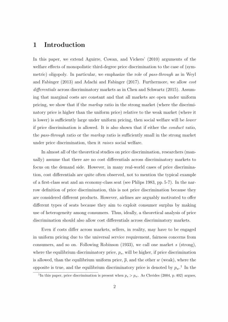
Note that Proposition 4 is stronger than Proposition 3. Similarly, as Figure 2

shows, the following proposition also holds.

Proposition 5. Given the IRC, if θsρsµs > θwρwµw, then price discrimination

lowers social welfare.

Again, Proposition 5 is stronger than Proposition 2. To see this, note that

θsρs =p− csp

(−pq

′s(p)

qs(p)

)ρs

22

Figure 1: Sufficient condition for price discrimination to raise social welfare:θwρwµw > θsρsµs for all q ∈ [0, q]. (Weaker sufficient condition (Prop 3):θ∗wρ

∗wµ∗w > θ∗sρ

∗sµ∗s)

23

Figure 2: Sufficient condition for price discrimination to lower social welfare:θsρsµs > θwρwµw

24

= (p− cs)(−q′s(p)

qs(p)

)ρs.

Now, by applying the implicit function theorem to F (p; q, cs) ≡ qs(p) − q + (p −cs)∂q

As (p, p)/∂ps, one obtains

ρs =∂p

∂cs(q, cs)

= −∂F/∂cs∂F/∂p

=∂xA,s(p, p)/∂ps

π′′s (p)

= − 1

π′′s (p)

qs(p)− qp− cs

,

which leads to

θsρs = − 1

π′′s (p)

qs(p)− qp− cs

(p− cs)(−q′s(p)

qs(p)

)=

q′s(p)

π′′s (p)

qs(p)− qqs(p)

.

Thus, it is shown that µs(q′s(p)/π

′′s (p)) > θsρsµs. Similarly, it is verified that θwρw >

q′w(p)/π′′w(p) because

θwρw =q′w(p)

π′′w(p)

qw(p) + q

qw(p).

In summary, if θsρsµs > θwρwµw holds, then µs · (q′s(p)/π′′s (p)) > µw · (q′w(p)/π

′′w(p)).

3.3 Consumer Surplus

One can extend the analysis above to consumer surplus. First, consumer surplus is

defined by replacing cm in W (r) by pm(r) to define

CS(r; cs, cw) = Us(qs(ps(r)))+Uw(qw(pw(r)))−2ps(r) ·qs(ps(r))−2pw(r) ·qw(pw(r)),

which implies that

CS ′(r)

2= ps(r) · q′s · p′s(r) + pw(r) · q′w · p′w(r)

−p′s(r) [ps(r) · q′s + qs]− p′w(r) [pw(r) · q′w + qw]

25

= − [p′s(r)qs + p′w(r)qw]

=

(− π

′′sπ′′w

π′′s + π′′w

)︸ ︷︷ ︸

>0

(qsπ′′s− qwπ′′w

).

=

(− π

′′sπ′′w

π′′s + π′′w

)︸ ︷︷ ︸

>0

[gs(ps(r), cs)− gw(pw(r), cw)]

where gm(p, cm) ≡ qm(p)/π′′m(p, cm). If gm(·, cm) is assumed to be decreasing, then

one can use a similar argument.

4 Concluding Remarks

This paper provides theoretical implications of oligopolistic third-degree price dis-

crimination with general nonlinear demands, allowing cost differentials across sep-

arate markets. In this sense, this paper, with the help of Weyl and Fabinger

(2013), synthesizes Aguirre, Cowan, and Vickers’ (2010) analysis of monopolistic

third-degree price discrimination with general demands and Chen and Schwartz’

(2015) analysis of monopolistic differential pricing, to extend them to the case of

symmetrically differentiated oligopoly.

If some of price-discriminating oligopolists merge into a single firm, what hap-

pens? Price discrimination is often neglected in a merger analysis. Traditionally, in

merger analyses, it has been considered as important to estimate own- and cross-

price elasticities. However, our theoretical analysis suggests that own- and cross-

price elasticities per se may not be so important in welfare evaluation. We conjecture

that our main thrust obtained under symmetric oligipoly, namely the fundamental

importance of the conduct index and the pass-through rate in welfare evaluation,

remains valid if asymmetric firms are allowed.

26

Appendix: Equivalence of Holmes’ (1989) and Our

Expressions for Q′(r)

Holmes (1989, p. 247), who assumes no cost differentials (c ≡ cs = cw) as in most of

the papers on third-degree price discrimination, also derives a necessary and suffi-

cient condition for Q′(r) > 0 under symmetric oligopoly. It is (using our notation)

written as:

ps − cq′s(ps)

· ddps

(∂xA,s(ps, ps)

∂pA

)− pw − cq′w(pw)

· d

dpw

(∂xA,w(pw, pw)

∂pA

)︸ ︷︷ ︸

adjusted-concavity condition (Robinson 1933)

+εCs (ps)

εIs(ps)− εCw(pw)

εIw(pw)︸ ︷︷ ︸elasticity-ratio condition (Holmes 1989)

> 0.

Recall that 1/θs− 1/θw = εCs /εIs− εCw/εIw. The first and the second terms in the

left hand side of Holmes’ (1989) inequality is rewritten as:

ps − cq′s(ps)

· ddps

(∂xA,s(ps, ps)

∂pA

)− pw − cq′w(pw)

· d

dpw

(∂xA,w(pw, pw)

∂pA

)= Lw(pw) ·

[(− pwq′w(pw)

)d

dpw

(∂xA,w(pw, pw)

∂pA

)]−Ls(ps) ·

[(− psq′s(ps)

)d

dps

(∂xA,s(ps, ps)

∂pA

)].

Now, it is also observed that

αFm − (1− θm)αCmθm

=αFmθm− ∂xB,m/∂pA

q′m

pm∂qB,m/∂pA

∂2xA,m∂pA∂pB

= −pmq′m

(−q′m

pm

αFmθm

+∂2xA,m∂pA∂pB

).

This shows that inequality (1) is another expression for Holmes’ (1989, p. 247)

inequality (9). To see this, note that

d

dpm

(∂xA,m(pm, pm)

∂pA

)=∂2xA,m∂p2

A

(pm, pm) +∂2xA,m∂pA∂pB

(pm, pm)

27

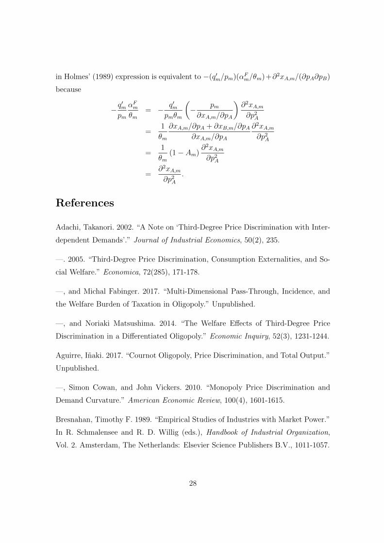
in Holmes’ (1989) expression is equivalent to −(q′m/pm)(αFm/θm)+∂2xA,m/(∂pA∂pB)

because

−q′m

pm

αFmθm

= − q′mpmθm

(− pm∂xA,m/∂pA

)∂2xA,m∂p2

A

=1

θm

∂xA,m/∂pA + ∂xB,m/∂pA∂xA,m/∂pA

∂2xA,m∂p2

A

=1

θm(1− Am)

∂2xA,m∂p2

A

=∂2xA,m∂p2

A

.

References

Adachi, Takanori. 2002. “A Note on ‘Third-Degree Price Discrimination with Inter-

dependent Demands’.” Journal of Industrial Economics, 50(2), 235.

—. 2005. “Third-Degree Price Discrimination, Consumption Externalities, and So-

cial Welfare.” Economica, 72(285), 171-178.

—, and Michal Fabinger. 2017. “Multi-Dimensional Pass-Through, Incidence, and

the Welfare Burden of Taxation in Oligopoly.” Unpublished.

—, and Noriaki Matsushima. 2014. “The Welfare Effects of Third-Degree Price

Discrimination in a Differentiated Oligopoly.” Economic Inquiry, 52(3), 1231-1244.

Aguirre, Inaki. 2017. “Cournot Oligopoly, Price Discrimination, and Total Output.”

Unpublished.

—, Simon Cowan, and John Vickers. 2010. “Monopoly Price Discrimination and

Demand Curvature.” American Economic Review, 100(4), 1601-1615.

Bresnahan, Timothy F. 1989. “Empirical Studies of Industries with Market Power.”

In R. Schmalensee and R. D. Willig (eds.), Handbook of Industrial Organization,

Vol. 2. Amsterdam, The Netherlands: Elsevier Science Publishers B.V., 1011-1057.

28

Chen, Yongmin, and Marius Schwartz. 2015. “Differential Pricing When Costs Dif-

fer: A Welfare Analysis.” RAND Journal of Economics, 46(2), 442-460.

Clerides, Sofronis K. 2004. “Price Discrimination with Differentiated Products: Def-

inition and Identification.” Economic Inquiry, 42(3), 402-412.

Czerny, Achim I., and Anming Zhang. 2015. “Third-Degree Price Discrimination

in the Presence of Congestion Externality.” Canadian Journal of Economics, 48(4),

1430-1455.

Dastidar, Krishnendu Ghosh. 2006. “On Third-Degree Price Discrimination in

Oligopoly.” The Manchester School, 74(2), 231-250.

Corts, Kenneth S. 1998. “Third-Degree Price Discrimination in Oligopoly: All-Out

Competition and Strategic Commitment.” RAND Journal of Economics, 29(2), 306-

323.

—. 1999. “Conduct Parameters and the Measurement of Market Power.” Journal of

Econometrics, 88(2), 227-250.

Flores, Daniel, and Vitaliy Kalashnikov. 2017. “Parking Discounts: Price Discrim-

ination with Different Marginal Costs.” Review of Industrial Organizaion, 50(1),

91-103.

Genesove, David, and Wallace P. Mullin. 1998. “Testing Static Oligopoly Models:

Conduct and Cost in the Sugar Industry, 1890-1914.” RAND Journal of Economics,

29(2), 355-377

Hendel, Igal, and Aviv Nevo. 2013. “Intertemporal Price Discrimination in Storable

Goods Markets.” American Economic Review, 103(7), 2722-2751.

Holmes, Thomas J. 1989. “The Effects of Third-Degree Price Discrimination in

Oligopoly.” American Economic Review, 79(1), 244-250.

Nahata, Babu, Krzysztof Ostaszewski, and P. K. Sahoo. 1990. “Direction of Price

Changes in Third-Degree Price Discrimination.” American Economic Review, 80(5),

1254-1258.

29

Phlips, Louis. 1983. The Economics of Price Discrimination. Cambridge, UK: Cam-

bridge University Press.

Robinson, Joan. 1933. The Economics of Imperfect Competition. London, UK:

Macmillan.

Schmalensee, Richard. 1981. “Output and Welfare Implications of Monopolistic

Third-Degree Price Discrimination.” American Economic Review, 71(2), 242-247.

Shapiro, Carl. 1996. “Mergers with Differentiated Products.” Antitrust, 10(2), 23-30.

Weyl. E. Glen, and Michal Fabinger. 2013. “Pass-through as an Economic Tool:

Principles of Incidence under Imperfect Competition.” Journal of Political Economy,

121(3), 528-583.

30