Output and Exports in Transition Economies: A Labor Management Model

Output and Exports in Transition Economies:A Labor Management Model1

John Bennett

University of Wales, Swansea, United Kingdom

Saul Estrin

London Business School, London NW1 4SA, United Kingdom

and

Paul Hare

Heriot–Watt University, Edinburgh, United Kingdom

Received November 20, 1997; revised November 16, 1998

Bennett, John, Estrin, Saul, and Hare, Paul—Output and Exports in Transition Econ-omies: A Labor Management Model

The behavior of an oligopolistic industry in a transition economy is analyzed, assuming thatthe firms are labor-managed and the economy is open to international trade. The output ofthese firms is assumed to be of lower quality than the output of Western firms. Cournotequilibrium in the presence of bottlenecks is derived. Such bottlenecks may be particularlydamaging because firms respond by cutting exports disproportionately. This may explain whycountries such as those in the former Soviet Union, which have faced serious supplybottlenecks, have failed to develop exports, while the economies of Central Europe, wherematerials are more freely available, have seen rapid export growth.J. Comp. Econom.,June1999,27(2), pp. 295–317. University of Wales, Swansea, United Kingdom; London BusinessSchool, London NW1 4SA, United Kingdom; and Heriot–Watt University, Edinburgh, UnitedKingdom. © 1999 Academic Press

Journal of Economic LiteratureClassification Numbers: D21, P31.

1. INTRODUCTION

In this paper we explore how important features of the transition process mightinteract to generate some of the enterprise supply behavior that we have seen in

1 The authors are grateful to John Bonin, James Maw, and to anonymous referees for detailed andvery helpful comments, which have enabled them to improve the paper. Earlier versions of the paperwere presented at a seminar at Heriot–Watt University and at a conference in Berlin organized by the

Journal of Comparative Economics27, 295–317 (1999)Article ID jcec.1999.1578, available online at http://www.idealibrary.com on

295 0147-5967/99 $30.00Copyright © 1999 by Academic PressAll rights of reproduction in any form reserved.

recent years. The first element of transition underlying our modeling is wide-spread insider ownership and control, which we formalize in the context of arevised Ward–Vanek model of labor-management. The second is the immediateopening of most transition economies to trade with OECD countries at very lowtariffs (World Bank, 1996; European Bank for Reconstruction and Development,1995, 1996, and 1997), with the resulting growth in exports, at least in much ofCentral Europe (Gros and Gonciarz, 1996). We bring these features together ina Cournot model with price discrimination between low and high quality prod-ucts; we assume that the output of firms in the transition economy is currently oflower quality than that of firms in Western economies. After characterizing theequilibrium for the firm and industry, we use the framework to consider animportant feature of economies in transition, i.e., bottlenecks in the supply of rawmaterials (Blanchard and Kremer, 1997; Roland and Verdier, 1997). We findthat, under these assumptions, constraints on materials supplies may lead enter-prises to cut exports before domestic production. Thus perversity in exportperformance may be a damaging implication of privatization policies that havefavored insiders. Moreover, we identify circumstances in which the effects arediscontinuous and large-scale: a small reduction in material supplies can lead toa large fall in exports. Thus the model predicts a relationship between supplybottlenecks and export performance. It may, therefore, explain why countries thathave faced supply problems, such as in the former Soviet Union, have failed toexpand manufacturing exports. This is in contrast to the economies of CentralEurope where materials are more freely available and export performance hastypically been very strong (European Bank for Reconstruction and Development,1997).

Our framework builds on several important strands of the earlier literature. Theoriginal labor-management model (Ward, 1958; Vanek, 1970; Meade, 1972)assumed the enterprise maximand to be average earnings per worker, but morerecent analysts have been critical of this assumption, particularly when employ-ment adjustment is a central concern (Ben-Ner and Estrin, 1991; Prasnikar et al.,1994; Bonin et al., 1993). We allow firms in transition to be motivated by aweighted product of employment and earnings (Blanchard, 1997), which nestswithin it the traditional self-management case.

Cournot equilibrium in the labor-managed economy is discussed, for example,in Hill and Waterson (1983); Neary (1984); Laffont and Moureaux (1985); andNeary and Ulph (1997)2 and mixed oligopoly models are treated in Cremer andCremer (1992) and Delboro and Rossini (1992). These papers assume incomemaximization and do not consider trade. Indeed, there is only a modest literature

Frankfurt Institute for Transformation Studies; comments from these meetings were also muchappreciated. The authors accept full responsibility for remaining deficiencies in the paper.

2 See also Sertel (1991) and Neary (1985) on monopolistic competition.

BENNETT, ESTRIN, AND HARE296

on labor-managed firms operating in foreign markets and in competition withprofit-maximizing firms (Mai and Hwang, 1989; Okuguchi, 1991; and Horowitz,1991). None of these papers covers the issue of price discrimination in a mixedoligopoly, which is at the core of this paper, nor in a revised-Ward framework.However, Katz and Berrebi (1980) provide the basic result for the price discrim-inating labor-managed monopolist under the assumption of income maximiza-tion.

The relevance of labor-management for the transition economies derives fromwidespread apparent insider control as well as ownership of enterprises. As notedby Earle and Estrin (1996), for the countries where data are available, it is clearthat reliance on mass privatization has led to dominant insider ownership in mostfirms. In countries as diverse as Romania, Poland, and Russia, the data suggestthat the bulk of the shares are owned by managers and workers who appear tocontrol the enterprise (Blasi et al., 1997). In addition, most analyses of state-owned firms in the immediate post-transition era (Pinto et al., 1993) have notedthat the collapse of effective control by the state allowed workers and managersto assume dominance over decision-making, a process that has proved extremelyhard to reverse. This had led many Western observers to regard the state sectorin transition economies as labor-managed (Commander and Coricelli, 1995;Blanchard, 1997). Especially in the early years of transition, it is these firms thatcontinue to provide the bulk of exports (European Bank for Reconstruction andDevelopment, 1995; Belka et al., 1995).3

Our main concern is to analyze the impact of supply bottlenecks in an openeconomy. The start of the transition typically involved simultaneous price andtrade liberalization (Gros and Steinherr, 1995), although the trade element washighly contentious (McKinnon, 1991). Domestic market structures were usuallyseverely imperfect (Estrin and Cave, 1993) and opening the economy to freetrade was seen as an important way to control domestic monopoly power (Liptonand Sachs, 1990). Hence, we have assumed an oligopolistic market structure forthe economy in transition, although our main results also apply for monopoly.Our analysis draws on the evidence that exports from transition economies havebeen concentrated at the lower quality end of the product range, while importshave included both high and low quality western products (Landesmannn andBurgstaller, 1998; Brenton and Gros, 1997). Moreover, while exports from sometransition economies have grown very rapidly (Carlin and Landesmann, 1997),

3 Our assumption that the enterprise sector in the transition economy can be regarded as a set oflabor-managed firms is clearly a stylization. In the past five years, some economies in transition,notably Poland and Hungary, have developed thriving private sectors, based onde novogrowth andon foreign direct investment respectively (Estrin, 1994, 1998). However, much of the growth in theprivate sector has come from small scale privatization in the retail, distribution, and services sectors;in most countries large scale industrial enterprises, which have traditionally supplied the bulk ofexports, have remained in state hands (World Bank, 1996; European Bank for Reconstruction andDevelopment, 1997).

OUTPUT AND EXPORTS IN TRANSITION 297

Aturupane et al. (1997) demonstrate that, in the period between 1990 and 1995,trade was predominantly in vertically differentiated products with the transitioneconomies exporting lower quality labor intensive products (European Bank forReconstruction and Development, 1997). In the work that follows, we model anindustry with a product produced at two quality levels, with firms in transitioneconomies producing the lower quality level and those in developed marketeconomies the higher one. Thus the transition economy is assumed to manufac-ture goods of lower quality, but not to import them. We abstract from other lowcost low quality suppliers who would, in practice, provide competition on theworld market in order to focus attention on the interaction between the West andthe transition economies. However, we reflect the broader availability of lowquality goods on the world market by assuming that their export price toexogenous to firms in the transition economies. Transition economies are alsoassumed to be price takers for the higher quality goods.

In the following section, we characterize the equilibrium for the firm and theindustry in a transition economy in the absence, and then in the presence, ofexports. We then compare the results with the capitalist case before analyzing, inthe third section, the impact of material supply bottlenecks on exports. Thebroader implications of our analysis are drawn in the final section.

2. THE BASIC MODEL

We abstract from questions of competition between transition and developedeconomies by assuming a single economy of each type. We thus assume twotypes of economy, developed and transition, manufacturing in an industry at twoquality levels. Firms in the transition economy produce at a lower quality level,while firms based in the developed market economy make the good at a higherquality level. For reasons discussed above, the transition economy exports thelower quality good and imports the higher quality one.4

Domestic demand in the transition economy for the lower quality good is

Q 5 a 2 p 1 gpf , a, g . 0, (1)

wherep is the unit price of the lower quality good, whilepf is the unit price ofthe higher quality good, in domestic currency. Also,a and g are constants,gbeing a measure of the cross-elasticity of demand between the two qualities ofgood. Asg goes to zero, product differentiation is greater. Equation (1) can berewritten

p 5 d 2 Q, (2)

4 If a group of transition economies were considered, the model would assume limited intragrouptrade flows, perhaps because of tariff and nontariff barriers. This conforms with the evidence; onceenergy and fuel trade is excluded, the flows of goods between transition economies are very modest(European Bank for Reconstruction and Development, 1995, 1996, 1997).


where

d ; a 1 gpf . (3)

Assuming that the import pricepf is given, the demand curve (2) facing domesticproducers in the transition economy is linear with a vertical intercept that isincreasing inpf. Furthermore, as noted above, we assume that domestic produc-ers are small in the export market and can sell unlimited quantities at the givendomestic currency unit pricepe.

For our specification of technology, we use a Leontief production function forconvenience. All the main results in this paper can be derived, although lesstractably, with a more general specification of technology. Moreover, the Leon-tief technology makes it particularly simple to introduce material supply con-straints in the subsequent section.5 Thus there areN ($1) domestic producers,each with production function

qi 5 min ai~l i , ki /bi!, ai , bi . 0, i 5 1, 2, . . . ,N. (4)

Firm i producesqi units of output employingl i workers. Its fixed capital stockis ki so that output can be no greater than the full capacity levelaiki /bi [ q# i .Firm i suppliesqh

i to the home market andqei to the export market, where

qi 5 qhi 1 qe

i . (5)

We assume each firmi to be labor-managed with a general objective function(Ben-Ner and Estrin, 1991) given by

ui 5 ~ y i ! s~l i ! 12s, 12 , s # 1, (6)

whereyi is net income per worker,

y i 5 ~ pqhi 1 peqe

i 2 rk i !/l i, (7)

andr is the positive rental on capital.6 If the weights in (6) is unity, we have theIllyrian firm of Ward (1958). Ifs , 1, we have a revised Illyrian firm in whichthere is a willingness to sacrifice some net income per worker for additionalemployment. Svejnar (1982) associates the weight in the utility function with theattitudes towards risk of the worker owners. We restricts . 1

2 in order to avoiddegenerate solutions.7

5 The Leontief assumption has some appeal in transition economies where the tradition of planningmay have reduced managerial experience with factor substitution (Blanchard, 1997).

6 The paymentr could be either a payment to the state for the use of the capital stock, along thelines of the former dividend tax in Poland, or a market-determined cost of capital for privatized firms.

7 Suppose that, in addition to the employment ofl i in production,l si workers are employed as

surplus, so that the objective function becomesui 5 ( yi )s(l i 1 l si ) 12s, whereyi 5 ( pqh

i 1 peqei 2

rk i )/(l i 1 l si ). Assume for now thats may take any value in the range (0, 1]. Thenui /l s

i 5 (1 2


2.1. Home Sales Only

In the home market, we assume that theN firms engage in Cournot compe-tition, whereas in the foreign market they face the fixed nominal pricepe.Suppose, first, that any firmi does not export. The Cournot solution in this caseis derived in Appendix A. Any firmi choosesqh

i to maximizeui , subject to(2)–(4), (6), and (7), given¥ jÞiqh

j and the constraintsqi # q# i andqei 5 0. The

solution is

qhi 5 min~qh

i , q# i !, (8)

where

qhi 5 1

2 $~1 2 s!D i 1 @~1 2 s! 2~D i ! 2 1 4~2s 2 1!rk i # 1/ 2% (9)

D i ; d 2 OjÞi

qhj . (10)

Given thats . 12, the square root in (9) is real. The firm producesqh

i unlessprevented from doing so by the capacity constraint. Ifs 5 1, i.e., no weight isput on employment in the objective function,qh

i 5 (rk i ) 1/ 2. Since the marginalrevenue product of labor in the home market is

MRPhi 5 ~D i 2 2qh

i !ai, (11)

the revised model nests the familiar labor-management case in whichyi 5MRPh

i . If, however,s , 1, with the capacity constraint not binding, it is shownin the Appendix8 that, provided inequality (A2) is satisfied, which is necessaryfor yi to be positive, the familiar utility maximizing result that, in equilibrium,average earnings exceed the marginal revenue product of labor holds.

Let l hi denote the employment corresponding to outputqh

i . The value ofl hi is

illustrated in Fig. 1, where the relationships shown are found by substituting (2),(6), (10), andqe

i 5 0 into (7) to obtain

y i 5 ~D i 2 ail i !ai 2 rk i/l i. (79)

Because of the Cournot assumption,D i is a parameter fori . The term (D i 2ai l i )ai is the derived residual demand for labor, which is plotted along with therectangular hyperbolark i /l i , the cost of capital per unit of labor.yh

i is positiveonly if l h0

i , l hi , l h1

i in the figure; this is equivalent to (A1) in the Appendix. If

2s) z ( pqhi 1 peqe

i 2 rk i )s z (l i 1 l si )22s. If s , 1

2, the value ofui /l si is therefore increasing in

l si , i.e., l s

i should be raised indefinitely. We exclude this degenerate solution by assumption.Furthermore, we also excludes 5 1

2, because the firm would be indifferent between all positive valuesof l s

i . Note that our argument here is independent of whether one or both ofqhi andqe

i are chosenfreely or whether they are determined by binding constraints.

8 Here, and throughout, we consider only those firms that produce a positive output in equilibrium.


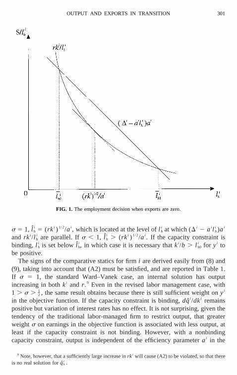
s 5 1, l hi 5 (rk i ) 1/ 2/ai , which is located at the level ofl h

i at which (D i 2 ai l hi )ai

and rk i /l hi are parallel. Ifs , 1, l h

i . (rk i ) 1/ 2/ai . If the capacity constraint isbinding, l h

i is set belowl hi , in which case it is necessary thatki /b . l h0

i for yi tobe positive.

The signs of the comparative statics for firmi are derived easily from (8) and(9), taking into account that (A2) must be satisfied, and are reported in Table 1.If s 5 1, the standard Ward–Vanek case, an internal solution has outputincreasing in bothki and r .9 Even in the revised labor management case, with1 . s . 1

2 , the same result obtains because there is still sufficient weight onyi

in the objective function. If the capacity constraint is binding,dqi /dki remainspositive but variation of interest rates has no effect. It is not surprising, given thetendency of the traditional labor-managed firm to restrict output, that greaterweight s on earnings in the objective function is associated with less output, atleast if the capacity constraint is not binding. However, with a nonbindingcapacity constraint, output is independent of the efficiency parameterai in the

9 Note, however, that a sufficiently large increase inrk i will cause (A2) to be violated, so that thereis no real solution forqh

i .

FIG. 1. The employment decision when exports are zero.


production function. Intuitively, this is because, on the one hand, the employmentobjective is independent ofai , while, on the other hand, maximization ofyi leadsto qh

i 5 (rk i ) 1/ 2, a solution that is independent ofai . However, capacity outputis increasing inai so that, if the capacity constraint binds,dqh

i /dai . 0.Finally, consider the effect of a greater value ofD i , the residual inverse

demand facingi . Suppose first that the capacity constraint is not binding. Ifs 51, there is no effect on output. In terms of Fig. 1, the residual demand for laborcurve, (D i 2 ai l h

i )ai shifts vertically upward so that the level ofl hi at which it is

parallel with (rk i ) 1/ 2/ai is unaffected. However, ifs , 1, so that the firm valuesemployment somewhat, a greater residual demand allows any given level ofemployment to be achieved at a smaller marginal cost in terms of earnings, andso output is raised. Referring back to the definitions of parameters in (1), (3), and(10), if s , 1 and the capacity constraint is not binding, employment is positivelyrelated to the demand intercepta, the measure of cross elasticity of demandg,and the import pricepf. If the capacity constraint is binding, however, output isindependent ofD i . From (10),dD i /dqh

i , 0 (i Þ j ). Therefore, the last row ofthe table implies that, provided the capacity constraint does not bind,dqh

i /dqhj ,

0 for s , 1, butdqhi /dqh

j 5 0 for s 5 1. We show in Appendix A thatd2qi /dqhj2

. 0 for s , 1.Given these results for the firm, we turn to the industry using the simplifying

assumption of a duopoly of identical firms. The solution is analyzed in AppendixB and illustrated in Fig. 2. Given that the capacity constraints are not binding,equilibrium outputs are

qh1 5 qh

2 5 $~1 2 s!d 1 @~1 2 s! 2d 2 1 4~2s 2 1!srk# 1/ 2%/ 2s, (12)

wherek1 5 k2 [ k. The figure is drawn on the assumption thats , 1, whileRi denotesi ’s reaction curve,qh

M is the monopoly output (N 5 1), andd 22(rk) 1/ 2 is the maximum value thatqh

i may take for the best responseq ih (i Þ j )

TABLE 1

Effects onqhi of Variation of Parameter Values

Parameter value raised qhi , q# i qh

i $ q# i

ki 1 1r 1 0s 2 0ai 0 1D i 1/0a 0

a 1 if s , 1, 0 if s 5 1.


to be real (see Appendix A).10 As shown in Appendix B, there is a unique stableequilibrium atE. Whens 5 1, each firmi has the straight line reaction curveq i

h

5 (rk) 1/ 2 and the equilibrium is atE9. If, for any se(12, 1], capacity constraints

enter the picture, the part of each reaction curve that involves output greater thanthe capacity level is simply deleted from the figure.

Consider the comparative statics of the industry equilibrium from Eq. (12).Any parameter change affects each reaction curve in the manner described inTable 1 for an individual firm. Thus, the industry equilibrium outputs adjust asshown in the table.

2.2. Sales to Both Home and Export Markets

We now consider exports at the level of the firm and the industry. With theintroduction of exports, firmi choosesqh

i andqei to maximizeui subject to Eqs.

10 It is possible thatd 2 2(rk) 1/ 2 , qhM, but this makes no difference to the solution. Note that for

qhj . d 2 2(rk) 1/ 2 the best response byi (i Þ j ) is not qh

i 5 0. Rather, there is no best responsedefined. Therefore, a segment ofRi coinciding with theqh

i -axis does not exist.

FIG. 2. Industry equilibrium when exports are zero.


(2)–(5) and (7), and given¥ jÞiqhj . SinceD i , as defined by Eq. (10), remains a

parameter for firmi , MRPhi is again given by Eq. (11), while firmi ’s marginal

revenue product in the export market is

MRPei 5 aipe . (13)

Given the set of outputs chosen by all other firmsj Þ i , firm i is, in effect, aprice-discriminating monopolist facing a downward-sloping (residual) marginalrevenue product curve in the home market and a horizontal marginal revenueproduct curve in the export market. As shown in Katz and Berrebi (1980), aninternal solution for firmi , if it exists, satisfies11

MRPhi 5 MRPe

i . (14)

The rationale for this result is that, for any total output produced byi , it is worthallocating supplies between the two markets so that total revenue is maximized.Substituting into (14) from (13) and then (11), firmi ’s supply of goods to thedomestic market is derived:

qhi 5 1

2 ~D i 2 pe!. (15)

Each unit supplied by firmi to the export market yields two benefits. First, itenables the fixed costrk i to be spread over more units of output. Second, itrequires the employment of additional labor, which is a benefit ifs , 1. Thus,given the determination ofqh

i by (15), firmi will devote all its remaining capacityto exports,

qei 5 q# i 2 qh

i . (16)

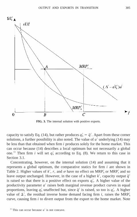
This solution is illustrated in Fig. 3. The relationships (D i 2 ai l hi )ai andrk i /l h

i

are reproduced from Figure 1, and MRPhi and MRPe

i are added. The marginalrevenue product curves intersect at point A so that the amount of labor devotedto supplying the home market is OB.12 The maximum amount of labor that canbe employed productively, i.e.,l i 5 q# i /ai , is shown as OC, so BC is the amountemployed in making exports.

Clearly, two types of corner solution are possible with MRPhi less than (greater

than) MRPei at the boundary. In these cases, firmi produces entirely for the

export (home) market. First, if MRPhi starts below MRPe

i , firm i produces onlyexports withqe

i 5 q# i . Second, suppose the case shown in Fig. 3 holds, but withthe amendment that point C lies to the left of B. Then the firm does not have the

11 Katz and Berrebi (1980) show that the price discriminating income maximizing monopolistproduces less than its profit maximizing counterpart, but may increase output with an increase inforeign demand.

12 Comparing Figs. 1 and 3, whether OB exceeds or falls short of (rk i ) 1/ 2/ai depends on how thefigures are drawn. Specifically, using (2), (4), (6), (11), and (14)–(16), it is found thatyi .MRPh

i (5MRPei ) as l h

i . (rk i ) 1/ 2/ai .


capacity to satisfy Eq. (14), but rather producesqhi 5 q# i . Apart from these corner

solutions, a further possibility is also noted. The value ofui underlying (14) maybe less than that obtained when firmi produces solely for the home market. Thiscan occur because (14) describes a local optimum but not necessarily a globalone.13 Then firm i will set qh

i according to Eq. (8). We return to this case inSection 3.1.

Concentrating, however, on the internal solution (14) and assuming that itrepresents a global optimum, the comparative statics for firmi are shown inTable 2. Higher values ofki , r , ands have no effect on MRPh

i or MRPei and so

leave output unchanged. However, in the case of a higherki , capacity outputq# i

is raised so that there is a positive effect on exportsqei . A higher value of the

productivity parameterai raises both marginal revenue product curves in equalproportions, leavingqh

i unaffected but, sinceq# i is raised, so too isqei . A higher

value ofD i , the residual inverse home demand facing firmi , raises the MRPhi

curve, causing firmi to divert output from the export to the home market. Note

13 This can occur becauseui is not concave.

FIG. 3. The internal solution with positive exports.


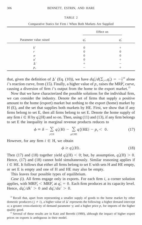
that, given the definition ofD i (Eq. (10)), we havedqhj /d(¥ jÞiqh

i ) 5 212

14 alonei ’s reaction curve, from (15). Finally, a higher value ofpe raises the MRPe

i curve,causing a diversion of firmi ’s output from the home to the export market.15

Now that we have characterized the possible solutions for the individual firm,we can consider the industry. Denote the set of firms that supply a positiveamount to the home (export) market but nothing to the export (home) market byH (E), and the set that supplies both markets by HE. First, we show that if anyfirms belong to set E, then all firms belong to set E. Denote the home supply ofany firmi [ H by qh

i (H) and so on. Then, using (11) and (13), if any firm belongsto set E the inequality in marginal revenue products reduces to

f ; d 2 Oj[H

qhj ~H! 2 O

g[HE

qhg~HE! 2 pe , 0. (17)

However, for any firmi [ H, we obtain

f $ qhi ~H!. (18)

Then (17) and (18) together yieldqhi (H) , 0; but, by assumption,qh

i (H) . 0.Hence, (17) and (18) cannot hold simultaneously. Similar reasoning applies ifi [ HE. It follows that either all firms belong to set E with sets H and HE empty,or set E is empty and one of H and HE may also be empty.

This leaves four possible types of equilibrium.Case (i).All firms engage only in exports. For each firmi , a corner solution

applies, with MRPhi , MRPe

i at qhi 5 0. Each firm produces at its capacity level.

Hence,dqei /dki . 0 anddqe

i /dai . 0.

14 Recall that, apart from representing a smaller supply of goods to the home market by otherdomestic producers (j Þ i ), a higher value ofD i represents the following: a higher demand intercepta; a greater cross-elasticity of demand parameterg; and a higher pricepf for imports of the higherquality good.

15 Several of these results are in Katz and Berrebi (1980), although the impact of higher exportprices on exports is ambiguous in their model.

TABLE 2

Comparative Statics for Firmi When Both Markets Are Supplied

Parameter value raised

Effect on

qhi qe

i

ki 0 1r 0 0s 0 0ai 0 1D i 1 2pe 2 1


Case (ii).All firms supply only the home market. For each firmi , either acorner solution applies, with the capacity constraint preventing Eq. (14) fromholding, or (14) is a local, but not a global, optimum. This case was examined inthe previous sub-section.

Case (iii).All firms supply both markets. Equation (14) holds and is a globaloptimum for each firmi . We saw from Table 2 thati ’s reaction curve is a straightline with dqh

i /d(¥ jÞiqhj ) 5 21

2. It follows that there is a unique stable equilibriumfor the industry. Furthermore, if all firms are homogeneous, the comparativestatics signs listed in Table 2 also apply at the industry level.

Case (iv).Some firms supply the home market only, because they face theconditions specified in Case (ii), while others supply both markets as specified inCase (iii). We illustrate this case with a simple example.

Assume that there are just two firms, 1 and 2, in the industry and that in theequilibrium 1 sells only in the home market, while 2 sells in both markets. Suchan equilibrium may occur, for example, ifq# 1 , q# 2; for specific conditions, seeAppendix C. Therefore,q1

h is given by Eq. (8), while, from (10) and (15), q2h 5

12(d 2 q1

h 2 pe). Solving for q1h andq2

h simultaneously, the comparative staticssigns listed in Table 3 are obtained. We discuss these signs briefly.

Suppose, first, that firm 1 produces at its capacity level in the equilibrium(q1

h 5 q# 1). If firm 1 has a larger capital stockk1, it produces more for thehome market, displacing some of the home sales by firm 2, which thereforesupplies more exports. If, instead, firm 2 has a larger capital stockk2, the soleeffect is that it exports more, by Eq. (16). Variations ofr and s have noeffect; but if the efficiency parameterai is greater (whena1 5 a2), firm 1supplies more to the home market and firm 2 supplies more to the exportmarket. Greater domestic demand, in the form of a higherd, causes firm 2 to

TABLE 3

Industry Comparative Statics When Firm 1 Supplies Only the Home Market,but Firm 2 Supplies Both Markets

Parametervalue raised

If q1h 5 q# 1 If q1

h 5 q1

qh1 qh

2 qh1 1 qh

2 qe2 qh

1 qh2 qh

1 1 qh2 qe

2

k1 1 2 1 1 1 2 1 1k2 0 0 0 1 0 0 0 1r 0 0 0 0 1 2 1 1s 0 0 0 0 ? ? ? ?a1 5 a2 1 0 1 1 0 0 0 1d 0 1 1 2 1/0* 1 1 2pe 0 2 2 1 1/0* 2 2 1

a 1 if s , 1, 0 if s 5 1.


switch sales from the foreign to the domestic market, while a higher foreignprice pe has the opposite effect.

Alternatively, supposeq1h 5 q1 in equilibrium. The effects of a largerk1

are qualitatively the same as in the previous paragraph because of thetraditional labor-management response of firm 1, not because firm 1 canproduce more output. For the same reason, variation ofr has effects of thesame sign as those resulting from variation ofk1. Nonetheless, an increase ink2 has the same type of effects as in the case whenq1

h 5 q# 1. However,variation ofs now affects the equilibrium, although the complexity of Eq. (9)and the interaction with firm 2’s behavior prevents us from signing the effect.Variation of a1 does not affectq1

h, since a1 does not enter Eq. (9) but, agreatera2 enables 2 to export more. An increase ind or pe has effects of thesame sign as in the case whenq1

h 5 q# 1, except in one respect. Since firm 1is not capacity-constrained, it can raiseqh

1 although it chooses not to do so ifs 5 1 as indicated in Eq. (9).

2.3. Comparison with Profit Maximizing Firms

It is natural to enquire how the results would be changed if all the firmsbehaved as capitalist firms. Therefore, we conclude this section by exploring thatcase and we then refer to it again below as a point of comparison. With capitalistfirms, each firmi maximizes profits,

p i ; pqhi 1 peqe

i 2 rk i 2 wl i, (69)

wherew is the externally given market wage rate. Again making the Cournotassumption, if firmi produces for the home market only, we have, parallel to (8),

qhi 5 min@1

2~Di 2 w/ai!, q# i#. (89)

When exports are introduced, however, the internal solution for capitalist firmssatisfies the same condition as in the labor-management case, i.e., equality ofmarginal revenue products, with exports again derived as a residual. There arealso corner solutions, with qh

i 5 0 if MRPei $ MRPh

i throughout, and withqei 5

0, either if the capacity constraint prevents attainment of the internal solution orif w . aipe, i.e., exports are loss-making.16

Turning to the industry level, (17) and (18) are again satisfied. Forcomparative purposes, we develop a two-firm example with firm 1 belong-ing to set H and firm 2 to set HE. If, in this example, it is the capacity

16 Here, as throughout the paper, we disregard firms that produce zero output in equilibrium. Also,note that if the industry contains some labor-managed and some capitalist firms, our analysis of thebehavior of an individual firm still holds. This is because we have made the Cournot assumption,which specifies that each firm takes the output of other firms as given regardless of the objectivefunctions used by the other firms in determining their outputs. (Cremer and Cre´mer, 1992).


constraint that prevents firm 1 from satisfying Eq. (14) and exporting, thenthe solution is identical to the case of labor management. The left-hand halfof Table 3 therefore applies. Alternatively, if firm 1 does not export becausew . a1pe, we have from (89) that qh

1 5 12(D

1 2 w/a1) and from (15) thatqh2

5 12(d 2 qh

1 2 pe). Therefore, using (10), we can solve for the equilibriumoutputs:

qh1 5 ~d 2 2w/a1 1 pe!/3

qh2 5 ~d 1 w/a1 2 2pe!/3. (19)

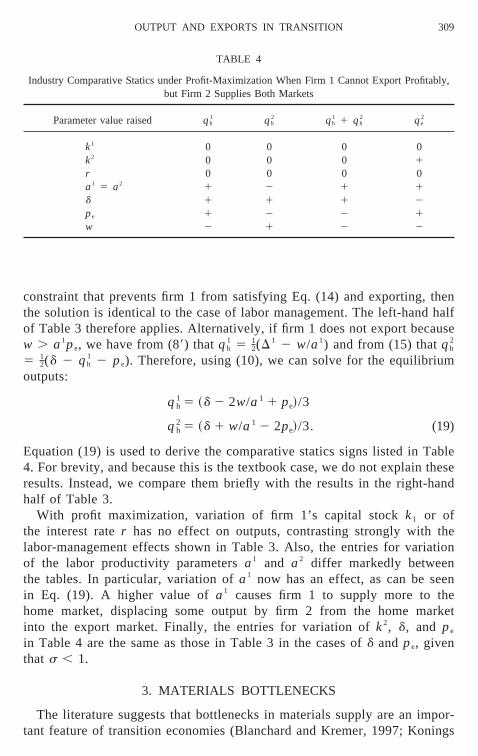
Equation (19) is used to derive the comparative statics signs listed in Table4. For brevity, and because this is the textbook case, we do not explain theseresults. Instead, we compare them briefly with the results in the right-handhalf of Table 3.

With profit maximization, variation of firm 1’s capital stockk1 or ofthe interest rater has no effect on outputs, contrasting strongly with thelabor-management effects shown in Table 3. Also, the entries for variationof the labor productivity parametersa1 and a2 differ markedly betweenthe tables. In particular, variation ofa1 now has an effect, as can be seenin Eq. (19). A higher value ofa1 causes firm 1 to supply more to thehome market, displacing some output by firm 2 from the home marketinto the export market. Finally, the entries for variation ofk2, d, and pe

in Table 4 are the same as those in Table 3 in the cases ofd and pe, giventhat s , 1.

3. MATERIALS BOTTLENECKS

The literature suggests that bottlenecks in materials supply are an impor-tant feature of transition economies (Blanchard and Kremer, 1997; Konings

TABLE 4

Industry Comparative Statics under Profit-Maximization When Firm 1 Cannot Export Profitably,but Firm 2 Supplies Both Markets

Parameter value raised qh1 qh

2 qh1 1 qh

2 qe2

k1 0 0 0 0k2 0 0 0 1r 0 0 0 0a1 5 a2 1 2 1 1d 1 1 1 2pe 1 2 2 1w 2 1 2 2


and Walsh, 1998). To examine this issue, assume that each firmi also usesa quantity of materialsmi in production. We can rewrite the productionfunction as

qi 5 min ai~l i, k i/bi, mi/c i !, ai, bi, c i . 0. (4a)

If pm is the unit price of materials, we can define

p i ; p 2 pmc i/ai; pei ; pe 2 pmc i/ai. (20)

For firm i , pi is the unit price received for supplying the home market, net ofmaterials costs, andpe

i is the similarly adjusted export price. Corresponding toEq. (7), we can write income per head as

y i 5 ~ p iqhi 1 pe

i qei 2 rk i !/l i. (7a)

With the firm maximizingui , whereyi is given by (7a), the analysis of Section2 still holds, with pi and pe

i replacingpi and pei , respectively. Each marginal

revenue product is reduced bypmci /ai . By the same token, the correspondinganalysis with capitalist firms goes through without change.

Suppose, however, that there is a constraint on materials supply to firmi ,mi # m# i . Assume first that, if the constraint is binding, firmi adjusts l i

accordingly so that no surplus labor is employed. This may be interpreted asthe case of chronic supply problems, that are long term and, therefore,anticipated. Because of the materials constraint,qi # aim# /ci [ q# m

i . If q# mi ,

q# i , which is the capacity constraint imposed by the limited capital stock, theresults of Section 2 still hold withq# m

i replacingq# i .17 An important implicationfor firms in set HE is that, since exports are determined as a residual, theintroduction of a binding materials constraint causes these firms to cut theirexports first.

This conclusion holds for both labor management and the capitalist version.However, there is another possibility that is more damaging to the transitioneconomy and occurs only with labor management. Because the local optimumdescribed by Eqs. (14)–(16) is not necessarily a global optimum, a smallreduction in the availability of materials can lead to a large reduction in exportsand output.

To illustrate this possibility, assume that theN firms in the industry arehomogeneous so that the superscripti can be omitted and that the constraint onoutput imposed by materials supply is always greater than the one imposed by thecapital stock. If an internal solution is achieved, Eqs. (14) through (16) yieldqh

17 Note, however, that a binding materials constraint, that limits output toq# mi , causesyi to be lower

than it would be with an alternative binding capital constraint that limits output toq# i whereq# i 5 q# mi .

When there are fewer materials available, the capital costrk i is unaffected; but when there is asmaller amount of capital,rk i is reduced.


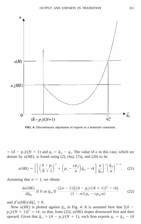
5 (d 2 pe)/(N 1 1) andqe 5 q# m 2 qh. The value ofu in this case, which wedenote byu(HE), is found using (2), (4a), (7a), and (20) to be

u~HE! 5 HFSd 2 pe

N 1 1D2

1 Spe 2cpm

a Dq# m 2 rkG a

q# mJ sSq# m

a D 12s

. (21)

Assuming thats , 1, we obtain

du~HE!

dq# mx 0 asq# m x

~2s 2 1!$@~d 2 pe!/~N 1 1!# 2 2 rk%

~1 2 s!~ pe 2 cpm/a!(22)

andd2u(HE)/dq# m2 . 0.

Now u(HE) is plotted againstq# m in Fig. 4. It is assumed here that [(d 2pe)/(N 1 1)]2 . rk, so that, from (22),u(HE) slopes downward first and thenupward. Given thatq# m . (d 2 pe)/(N 1 1), each firm exportsqe 5 q# m 2 (d

FIG. 4. Discontinuous adjustment of exports to a materials constraint.


2 pe)/(N 1 1).18 As q# m 3 (d 2 pe)/(N 1 1) from above,qe 3 0, so thatu(HE) 3 u0(HE) in the figure. However, ifqe 5 0, i.e., with home sales only,it is not always optimal to setqh 5 q# m. Rather, Eq. (8) will be satisfied, althoughit must be adjusted to take into account the materials constraint, i.e.,qh 5min(qh, q# m). The value ofu in this solution for home sales only is denoted byu(H) in the figure. Generally,u(H) . u0(HE). The value ofq# m at whichu(HE)5 u(H) is denoted byq# *m. It can be seen that, ifq# m . q*m, marginal reductionsin q# m cause marginal reductions in exports. However, ifq# m 5 q*m, a marginalreduction inq# m causes each firm to switch to supplying the home market only.

Since, as we explain below, the discontinuity of adjustment results from thesimultaneous pursuit of the objectives of raising income per head and raisingemployment, rather than from strategic interaction, we simplify by settingN 51. Suppose thats 5 0.75,d 5 12, pe 5 4, r 5 0.1, k 5 10 andpm 5 a 5c 5 1. Thereforem# is measured in the same units asq# m. It is found that (d 2pe)/(N 1 1) 5 4, while the minimum point on theu(HE)-curve occurs atq# m 510. For optimal choice with home sales only, we haveqh ' 3.16 andu(HE) '6.06, from which we obtainq# * ' 32.42.Hence, if there is a marginal reductionof m# and, therefore, ofq# m below 32.42, a firm’s output will fall from 32.42 to3.16 with exports falling from 28.42 to 0 and home sales falling from 4 to 3.16.

This type of discontinuous adjustment can be explained intuitively. Suppose afirm were to sell only in the home market. For reference, denote the values ofy,l , andu it therefore achieves byy, l , andu# , respectively. However, if MRPe .y, all possible units of exports are always worth producing because they raiseboth y and l , and thereforeu, abovey, l , and u, respectively. Discontinuousadjustment does not occur in this case. However, now suppose that MRPe , y,in which case any exporting reduces earnings belowy. As a result, the export ofa small amount may not be advantageous to the firm compared to not exportingat all, because the corresponding small increase in employment may not com-pensate the firm, in utility terms, for the lower earnings. However, if largeramounts of exports can be made, there is a correspondingly large increase inemployment. Since there is a lower bound to the value that earnings may take, thel -component of utility eventually dominates. A large enough quantity of exportsis worth undertaking. Note that this argument rests on the assumption that thereis some weight on employment in the utility function. In the Ward model, withs 5 1, there is no discontinuous adjustment.

Now assume instead that the materials shortage is not foreseen. We maysuppose thatl i is already fixed, as specified in Section 2, for the periodconcerned. If firmi belongs to set H or set E, it merely reduces its supply to thegiven market. However, if firmi belongs to HE, it must decide how to apportionthe cut in its supply between the markets. Since MRPh

i is downward-sloping but

18 In Fig. 4, we have also assumed that (d 2 pe)/(N 1 1) is to the left of the minimum of theu(HE) curve. Reversal of this assumption would not affect our conclusions significantly.


MRPei is horizontal, exports will be cut first, as in the case of anticipated materials

shortage. However, the possibility of discontinuous adjustment does not arise. Interms of the argument of the previous paragraph, if exporting causes a fall inyi ,there cannot be a compensating rise inl i , for l i is fixed when the relevantdecision is made.19

To summarize, we have found that the shortage of materials in a transitioneconomy, whether anticipated by firms or not, tends to affect exports dispropor-tionately. Part of our argument depends on smooth adjustment and results fromthe relative slopes assumed for MRPh

i and MRPei . This part of the argument holds

equally for capitalist firms and labor-managed ones. However, we have identifiedthe possibility of discontinuous adjustment that has potentially more damagingeffects for the transition economy. This cannot occur with capitalist firms. Itdepends on labor management and can occur only if some weight is put onemployment in the utility function and if the materials shortage is anticipated.20

4. CONCLUSIONS

We have analyzed the behavior, at the level of firms and the industry, of atransition economy open to international trade. Our key assumptions are anoligopolistic market structure, in which firms follow a Cournot decision rule,there is product differentiation among firms in transition economies supplyingoutput at lower quality than that of Western firms and there is labor management.The first two assumptions are not particularly strong since all transition econo-mies emerged from central planning with a few large firms in each sector and anorientation to industrial production with limited concern for product quality orinternational standards. The assumption of labor management is potentially moredebatable. Mass privatization has provided insiders, notably workers, with dom-inant ownership stakes in most transition countries. Our concern with output andemployment adjustment, given the high unemployment in many transition econ-omies (Commander and Coricelli, 1995), leads us to use a revised labor-management model that includes employment explicitly as an enterprise objec-tive. We also provide comparisons with the traditional capitalist firm.

From the perspective of policy, the most significant results relate to the impactof material supply bottlenecks. These were very common in the early years of

19 With an unanticipated shock, Eq. (21) applies with minor amendments. In the termsa/q# m andq# m/a, the q# m is replaced byq# ; but the other appearance ofq# m in (21) still applies.

20 Another constraint that may affect a firm relates to inexperience in export marketing and the lackof relevant international contacts (Cooper and Ga´cs, 1997). Firmi may face the export constraint,qe

i

# q# ei . However, given that the firm anticipates this constraint when it makes its production decisions

and assuming that in the absence of the constraint the firm would belong to set HE, few clear-cutresults emerge. The reason for this is that, whenqe

i 5 q# ei , the denominator of net earnings per head

yi becomesl hi 1 q# e

i /ai . Unless the restrictions 5 1 is made, this complicates the analysis in that thecomparative statics are indeterminate.


transition and we find that they can hinder a country’s export efforts. Suchshortages, whether or not they are anticipated, are shown to have a dispropor-tionate effect on exports. These bottlenecks have been especially serious in theformer Soviet Union and may still be so in the successor states. The logic of thispaper suggests that these material supply problems might help to explain therelatively poor export performance of manufacturing in Russia and elsewhere inthe former Soviet Union relative to the Central European economies, which haveexperienced fewer material supply bottlenecks.

APPENDIX A. THE GENERAL CASE FOR HOME SALES ONLY

Setqei 5 0 in (7). Using (2), (7), and (10),yi 5 2[(qh

i ) 2 2 D iqhi 1 rk i ]/ l i .

Given thatrk i . 0, it follows thatyi . 0 if

12$D

i 2 @~D i ! 2 2 4rk i # 1/ 2% , qhi , 1

2 $D i 1 @~D i ! 2 2 4rk i # 1/ 2%. (A1)

We assume that the square root here is real, i.e., that

~D i ! 2 2 4rk i . 0. (A2)

Also, we restrict our discussion throughout to cases in which (A1) is satisfied.Ignoring the capacity constraint, consider the choice of optimalqh

i under theCournot assumption. From (2), (6), (7), and (10) and given thatyi . 0, thefirst-order condition is Eq. (9) in the text, but with the square root taking eithersign. However, only the positive square root satisfies the second-order condition.When the capacity constraint is also considered, Eq. (8) is obtained. However, itmust also be taken into account that, given that there are fixed capital costs, thecapacity constraint may be so tight that (A1) cannot be satisfied, in which casea real solutionqh

i does not exist.Using (2), (4), (7), and (11), we find that MRPh x yi as (rk i ) 1/ 2 x qh

i .Assuming thatqh

i 5 qhi , substitution from Eq. (8) then yields

MRPhi x y i as 4rk i~1 2 s! 2 x ~D i ! 2~1 2 s! 2. (A3)

Hence, ifs 5 1, MRPhi 5 yi ; but if s , 1, (A2) and (A3) yield MRPh

i , yi .Finally, consider howqh

i is related toqhj . From (9), if s 5 1, the two are

independent. However, suppose thats , 1; from (9),

dqhi

dqhj 5 21

2 ~1 2 s!$1 1 ~1 2 s!D i @~1 2 s! 2~D i ! 2 1 4~2s 2 1!rk i # 21/ 2% , 0

~s , 1!

d2qhi

dqhj 5 2~2s 2 1!~1 2 s! 2rk i @~1 2 s! 2~D i ! 2 1 4~2s 2 1!rk i # 23/ 2 . 0.

(A4)


APPENDIX B. INDUSTRY EQUILIBRIUM FOR HOME SALES ONLY(N 5 2)

Substituting into (A2) from (10), ifN 5 2, a real solution forqhi is found only

if qhj # d 2 2(rk) 1/ 2 ( j Þ i ). Substituting into (9), ifqh

j 5 d 2 2(rk) 1/ 2, thenqh

i 5 (rk) 1/ 2 (i Þ j ).From (9):

~qhi ! 2 2 ~1 2 s!~d 2 qh

j !qhi 1 ~1 2 2s!rk 5 0, i Þ j . (A5)

Write (A5) for i 5 1, j 5 2 first and then forj 5 1, i 5 2. Subtracting thesecond of the resulting equations from the first, we obtain (qh

1 2 qh2)[qh

1 1 qh2 2

d(1 2 s)] 5 0. Hence, in equilibrium, either (a)qh1 5 qh

2 or (b)qh1 1 qh

2 5 d(1 2s). However, substituting (b) into (A5) fori 5 1, j 5 2 first and then forj 51, i 5 2, we obtainqh

1 5 qh2. Therefore (b) reduces to (a) and the unique real

solution isqh1 5 qh

2.From (A5), along firm 1’s reaction curveR1,

dqh1/dqh

2 5 2~1 2 s!qh1/@2qh

1 2 ~1 2 s!~d 2 qh2!#. (A6)

Suppose thats , 1. From (A4), we havedqh1/dqh

2,0 and so, in (A6), 2qh1 2

(1 2 s)(d 2 qh2) . 0. Using qh

1 5 qh2, we obtain from (A6) that

dqh1/dqh

2 x 21 asqh1 x ~1 2 s!d/ 2. (A7)

Writing (9) with N 5 2 andqh1 5 qh

2 and using the resulting equation to eliminateqh

1 in the second inequality in (A7), we obtaindqh1/dqh

2.21. Similarly, dqh2/

dqh1.21 and the equilibriumqh

1 1 qh2 is stable. From (A5), this solution is Eq.

(12) in the text.

APPENDIX C. CONDITIONS FOR INDUSTRY EQUILIBRIUMIN CASE (iv)

By assumption, firm 1 belongs to set H and firm 2 to set HE. Hence, MRPh1 .

MRPe1 and MRPh

2 5 MRPe2. Therefore, from (10), (11), and (13),d 2 qh

2 2 2qh1

. pe andd 2 qh1 2 2qh

2 5 pe. Consequently,qh2 . qh

1, i.e., (d 2 qh1 2 pe)/ 2 .

qh1, which reduces tod 2 pe . 3qh

1. Writing l [ qh1/q# 1, we have

d 2 pe . 3lq# 1. (C1)

Sinceqh2 5 (d 2 qh

1 2 pe)/2 andqe2 . 0, we haveq# 2 . (d 2 qh

1 2 pe)/2, whichcan be rewritten as

2q# 2 1 lq# 1 . d 2 pe . (C2)


Writing q# 2 [ mq# 1 and combining (C1) and (C2), we obtain

2m 1 l . ~d 2 pe!/q#1 . 3l. (C3)

For (C3) to hold, it is necessary thatm . l, i.e., thatq# 2 . qh1. Specifically, ifqh

1

5 q# h1 in (8), it is necessary thatm . 1, i.e., that capacity output be greater for firm

2 than firm 1.

REFERENCES

Aturupane, Chonira, Djankov, Simeon, and Hoekman, Bernard, “Determinants of Intra-industryTrade between East and West Europe.” London: Centre for Economic Policy Research, 1997.

Belka, Marek, Estrin, Saul, Schaffer, Mark, and Singh, Inderjit, “Enterprise Adjustment in Poland:Evidence from a Survey of 200 Private, Privatized and State-Owned Firms.” Centre for EconomicPerformance Discussion Paper 233, London: London School of Economics, Apr. 1995.

Been-Ner, Avner, and Estrin, Saul, “What Happens when Unions Run Firms? Unions as EmployeeRepresentatives and as Employers,”J. Comp. Econ.15, 1:65–87, Mar. 1991.

Blanchard, Olivier,The Economics of Post-Communist Transition.Clarendon Lectures in Economics,Oxford: Clarendon, 1997.

Blanchard, Olivier, and Kremer, Michael, “Disorganization.”Q. J. Econ.112, 4:1091–1126, Nov.1997.

Blasi, Josef R., Kroumova, Maya, and Kruse, Douglas,Kremlin Capitalism.Ithaca: Cornell Univ.Press, 1997.

Bonin, John P., Jones, Derek C., and Putterman, Louis, “Theoretical and Empirical Studies of ProducerCooperatives—Will Ever the Twain Meet?”J. Econ. Lit.31, 3:1290–1320, Sept. 1993.

Brenton, Paul, and Gros, Daniel, “Trade Reorientation and Recovery in Transition Economies.”Oxford Rev. Econ. Policy13, 2:65–76, Summer 1997.

Carlin, Wendy, and Landesmann, Michael, “From Theory into Practice? Restructuring and Dyna-mism in Transition Economies.”Oxford Rev. Econ. Policy13, 2:77–105, Summer 1997.

Commander, Simon, and Coricelli, Fabrizio, Eds.,Unemployment Restructuring and the LaborMarket in Eastern Europe and Russia.Economic Development Institute (EDI) DevelopmentStudies, Washington DC: World Bank, 1995.

Cooper, Richard N., and Ga´cs, Janos, “Impediments to Exports in Small Transition Economies.”MOCT–MOST7, 2:5–32, 1997.

Cremer, Helmuth, and Cre´mer, Jacques, “Duopoly with Employee-Controlled and Profit-MaximizingFirms: Bertrand vs Cournot Competition.”J. Comp. Econ.16, 2:241–258, June 1992.

Delbono, Flavio, and Rossini, Gianpaolo, “Competition Policy vs Horizontal Merger with Public,Entrepreneurial, and Labor-Managed Firms.”J. Comp. Econ.16, 2:226–240, June 1992.

Earle, John, and Estrin, Saul, “Employee Ownership in Transition.” In Frydman, Roman, Gray,Cheryl, and Rapaczynski, Andrzej Eds.,Corporate Governance in Central Europe andRussia. Vol. 2. Insiders and the State.Budapest: Central European University Press, 1996.

Estrin, Saul, Ed.,Privatization in Central and Eastern Europe.London: Longman, 1994.Estrin, Saul, “Privatization.” In Peter Boone, Stanislaw Gomulka and P. Richard Layard,Emerging

from Communism: Lessons from Russia, China, and Eastern Europe.Cambridge, MA: MITPress, 1998.

Estrin, Saul, and Cave, Martin, Eds.,Competition and Competition Policy: A Comparative Analysisof Central and Eastern Europe.London: Pinter, 1993.

European Bank for Reconstruction and Development,Transition Report.London: European Bank forReconstruction and Development, 1995, 1996, 1997.

Gros, Daniel, and Gonciarz, Andrzej, “A Note on the Trade Potential of Central and Eastern Europe.”Eur. J. Polit. Econ.12, 4:709–721, Dec. 1996.


Gros, Daniel, and Steinherr, Alfred,Winds of Change: Economic Transition in Central and EasternEurope.London: Longman, 1995.

Hill, Martyn, and Waterson, Michael, “Labor-Managed Cournot Oligopoly and Industry Output.”J. Comp. Econ.7, 1:43–51, March 1983.

Horowitz, Ira, “On the Effects of Cournot Rivalry between Entrepreneurial and Cooperative Firms.”J. Comp. Econ.15, 1:115–121, March 1991.

Katsoulacos, Yannis, “Firms’ Objectives in Transition Economies.”J. Comp. Econ.19, 3:392–409,Dec. 1994.

Katz, Eliakim, and Berrebi, Z. M., “On the Price Discriminating Labour Cooperative.”Econ. Lett.6,99–102, 1980.

Konings, Josef, and Walsh, Patrick, P., “Disorganization in the Transition Process: Firm LevelEvidence from Ukraine.” Discussion Paper 1928, London: Center for Economic PolicyResearch, 1998.

Laffont, Jean-Jacques, and Moreaux, Michel, “Large-Market Cournot Equilibria in Labour-ManagedEconomies.”Economica52, 26:153–165, May 1985.

Landesmann, Michael, and Burgstaller, Johann, “Vertical Product Differentiation in EU Market; TheRelative Position of Eastern European Producers.”Russ. East Eur. Finance Trade34,1:32–78, Jan.–Feb. 1998.

Lipton, David, and Sachs Jeffrey, “Creating a Market Economy in Eastern Europe: The Case ofPoland.”Brookings Pap. Econ. Activity1:75–133, 1990.

Mai, Chao-Cheng, and Hwang, Hong, “Export Subsidies and Oligopolistic Rivalry between Labor-Managed and Capitalist Economies.”J. Comp. Econ.13, 3:473–480, Sept. 1989.

McKinnon, Roland, I.,The Order of Economic Liberalization: Financial Control in the Transition toa Market Economy.Baltimore, MD: Johns Hopkins Univ. Press, 1991.

Meade, James E., “Theory of Labor-Managed Firms and of Profit Sharing.”Econ. J.82, 325:402–428, Supplement, March 1972.

Mejstrik, Michal, Ed.,The Privatization Process in East-Central Europe. Evolutionary Process ofCzech Privatization,International Studies in Economics and Econometrics, Vol. 36. Dordre-cht: Kluwer Academic, 1997.

Neary, Hugh M., “Labor-Managed Cournot Oligopoly and Industry Output: A Comment.”J. Comp.Econ.8, 3:322–327, Sept. 1984.

Neary, Hugh M., “The Labor-Managed Firm in Monopolistic Competition.”Economica52,28:435–447, Nov. 1985.

Okuguchi, Koji, “Labor-Managed and Capitalistic Firms in International Duopoly: The Effects ofExport Subsidy.”J. Comp. Econ.15, 3:476–484, Sept. 1991.

Pinto, Brian, Belka, Marek, and Krajewski, Stefan, “Transforming State Enterprises in Poland: Evidenceon Adjustment by Manufacturing Firms.”Brookings Pap. Econ. Activity1:213–261, 1993.

Prasnikar, Janez, Svejnar, Jan, Michajlek, Dubravko, and Prasnikar, Vesna, “Behavior of Participa-tory Firms in Yugoslavia: Lessons for Transforming Economies.”Rev. Econ. Statist.76,4:728–741, Nov. 1994.

Roland, Ge´rard, and Verdier, Thiery, “Transition and the Output Fall.” Research Discussion Paper1636, London: Center for Economic Policy Research, May 1997.

Sertel, Murat R., “Workers’ Enterprises in Imperfect Competition.”J. Comp. Econ.15, 4:698–710,Dec. 1991.

Svejnar, Jan, “On the Theory of a Participatory Firm,”J. Econ. Theory27, 2:313–330, Aug. 1982.Vanek, Jaroslav,The General Theory of Labor-Managed Market Economies.Ithaca, NY: Cornell

Univ. Press, 1970.Ward, Benjamin M., “The Firm in Illyria: Market Syndicalism.”Am. Econ. Rev.48,4:566–589, Sept.

1958.World Bank,World Development Report 1996: From Plan to Market.Oxford/New York: Oxford

Univ. Press for the World Bank, 1996.


Documents

Output and Exports in Transition Economies: A Labor Management Model