For comments, suggestions or further inquiries please contact:

Philippine Institute for Development Studies Surian sa mga Pag-aaral Pangkaunlaran ng Pilipinas

The PIDS Discussion Paper Series constitutes studies that are preliminary and subject to further revisions. They are being circulated in a limited number of copies only for purposes of soliciting comments and suggestions for further refinements. The studies under the Series are unedited and unreviewed.

The views and opinions expressed are those of the author(s) and do not necessarily reflect those of the Institute.

Not for quotation without permission from the author(s) and the Institute.

The Research Information Staff, Philippine Institute for Development Studies 18th Floor, Three Cyberpod Centris – North Tower, EDSA corner Quezon Avenue, 1100 Quezon City, Philippines Tel Numbers: (63-2) 3721291 and 3721292; E-mail: publications@mail.pids.gov.phOr visit our website at https://www.pids.gov.ph

Outlook for the Philippine Economy and Agro-Industry to 2030:

The Role of Productivity Growth

DISCUSSION PAPER SERIES NO. 2017-30

Roehlano M. Briones

November 2017

1

Outlook for the Philippine Economy and Agro-industry to 2030:

The Role of Productivity Growth

Roehlano M Briones

Research Fellow II, PIDS

15 November 2017

Abstract

The main driver of long run economic growth is total factor productivity. Among the basic

sectors, namely agriculture, industry, and services, inclusiveness of economic growth

depends most importantly on agriculture. This study provides growth projections for the

Philippine agriculture based on growth in productivity differentiated by basic sector, using a

computable general equilibrium (CGE) model.

Scenario analysis finds that the current policy thrust for agriculture of subsidizing capital cost

slightly accelerates growth of agriculture, but slows down overall growth by reducing capital

formation. Meanwhile, maintaining productivity growth for industry-service at trend,

notwithstanding weak growth of agriculture, suffices to reach government plan targets.

Productivity growth of agriculture impacts strongly on agriculture itself, but not on the

industry-services sectors; conversely, productivity growth in the latter strongly impacts on

itself and GDP, but not on agriculture.

The study suggests that policies emphasize the acceleration of productivity growth in the long

run across all sectors, but especially in agriculture. Currently, forward and backward linkages

of agriculture matter little to economic growth; increasing growth interactions across the

basic sectors.

Key words: Philippine economy, agriculture, agro-industry, computable general equilibrium,

total factor productivity, growth projections

2

1. INTRODUCTION

According to the Philippine Development Plan (PDP), the Philippines aims at becoming an

upper middle income country by 2022, with an income of $5,000 (NEDA, 2017). This

represents a 41 percent jump over its 2015 level of $3,550. Overall poverty is seen to decline

from 21.6 percent in 2015, to only 14.0 percent in 2022.

The basic sectors of an economy are agriculture, industry, and services. Among the basic

sectors, agriculture plays an important role in reducing poverty. Up to two-thirds of all poor

workers in the country are agricultural workers (Briones, 2016). In 2016, its share in GDP

was down to down to 8.8 percent, while employing as much as 29 percent of all workers;

hence labor productivity in agriculture is low compared with the other basic sectors. A more

inclusive set of policies are needed to secure the participation of agriculture-dependent

households in the economic mainstream.

Growth in agriculture has significantly lagged that of the other basic sectors. The average

growth in agriculture over the period 2011 to 2016 was just 2 percent, while that of industry

and services was 7 percent. Agricultural wages have also been depressed, growing by only

0.2 percent annually from 2002 to 2012 in real terms. Poor performance of agriculture is

worrisome in view of rising food needs of a growing population, the precarious state of the

country’s natural resource base, and the adverse impacts of climate change (Thomas et al.

2015).

In the short run, macroeconomic aggregates related to demand, the fiscal balance, and the

balance of payments, are important drivers of gross domestic product (GDP). As the

economy maintains its sound macroeconomic fundamentals i.e. a manageable fiscal deficit,

low inflation, and stable balance of payments, the attention of policymakers naturally turns to

the supply side of the economy. In the long run, economic growth ultimately depends on

supply factors.

Expansion of supply involves increases in primary inputs (labor and capital), and

technological progress, as measured by growth in total factor productivity (TFP). Labor

supply depends on population growth (labor force participation being constant), while capital

accumulation depends savings out of current income. On the other hand, growth in TFP

depends on innovation, adoption of new technologies and systems, and closure of technical

efficiency gaps. As a source of overall growth in the long run, growth in TFP shows greater

potential than growth in factors of production.

However, policy support, especially to agriculture, appears biased towards raising private

returns to capital, rather than in boosting TFP. In 2012 – 14, agricultural price support and

input subsidy was estimated to be as large as 25% of the value of agricultural production.

General support for public goods (more closely associated with productivity enhancement)

accounted just 4 percent (OECD, 2017). Current budgetary priorities continue to emphasize

input subsidies for credit, and farm machinery, as well as irrigation services, agricultural

insurance, and seeds.

This study aims to implement an updated set of projections for the Philippine agriculture in

the context of growth of the economy and of agro-industry, based on direct and indirect

impacts of TFP growth. The latter is applied differentially to agriculture, industry, and

services. The following key questions are posed:

3

What productivity trends underlie the expected trajectory of economic growth of the

country? To what extent does growth depend on current policy priorities, i.e.

subsidies?

What are the implications of acceleration and slowdown of productivity growth in

agriculture for output, consumption, and wages?

What are the implications of acceleration productivity growth in industry and services

for output, consumption, and wages?

The issues will be investigated using a computable general equilibrium (CGE) model, of a

standard structure. Data is derived from a social accounting matrix (SAM) of the Philippine

economy, reflecting most recent available information on inter-industry flows and national

accounts. Of special interest in the study is the indirect impact across sectors, for which the

SAM is especially suited. If indirect impacts are found to be strong, then industry, services,

and agriculture are already in well-integrated value chains; growth in one basic sector will

contribute significantly to growth in the other basic sectors. However, if indirect impacts are

found to be weak, then the current structure of the economy implies little role for forward and

backward linkages in future economic growth. This may highlight the need closer integration

of agriculture with other basic sectors through an agricultural value chain approach.

4

2. THE MODEL

Overview of AMPLE-CGE

For this study, the Agricultural Model for PoLicy Evaluation (AMPLE), described in Briones

(2014), was extended into an economywide version, called AMPLE – CGE. The agricultural

sectors of AMPLE-CGE are drawn from those of AMPLE. To this is added the industry and

service sectors (Table 1); the latter are referred to jointly as industry-service.

The AMPLE-CGE follows a conventional structure for computable general equilibrium

models, such as described in Lofgren, Harris, and Robinson (2002), which in turn draws from

Dervis, de Melo, and Robinson (1982); see also Robichaud et al (2012). The model is coded

and solved in Generalized Algebraic Modeling System (GAMS) using the CONOPT3 Solver.

The institutions of the AMPLE-CGE are: i) households, divided into rural and urban; ii)

business firms; iii) government; and iv) rest of the world. Final demands are, respectively:

consumption; investment; government consumption; and exports. Imports are subtracted to

net out purchased goods not produced domestically.

Factors of production are agricultural labor, industry-service labor, and capital. The types of

labor are segmented into their own factor markets; hence wages are set independently across

the labor categories. Capital is malleable across sectors and allocated to equalize value of

marginal product with the price (i.e. rental cost) of capital.

Consumption is modeled as a linear expenditure system (LES), as in Robichaud et al (2012).

Calibration is implemented with assumed values of elasticities for income and own-price.

Total investment demand equals total savings, allocated across sectors based on fixed

expenditure shares. Total government consumption is exogenous, and is likewise allocated

across sectors according to fixed expenditure shares. Intermediate demand among sectors is

modeled as a fixed proportions (Leontieff) system. Demand is allocated between

domestically-produced goods and imports following an Armington-type allocation, from

which is inferred the import demand. World prices are fixed; government collects import

tariffs.

Value added is a fixed proportion of gross output. Production of value added uses capital and

labor; the latter is divided into agricultural labor and industry-services labor. The labor types

are viewed as distinct and non-substitutable. The production function mapping value added to

capital and labor combinations adopts a constant elasticity of substitution (CES) form.

Calibration of production function parameters involves estimates of elasticities of

substitution, based to some extent on past studies. Government collects indirect taxes based

on value added.

Rural and urban households pay income taxes as a fixed proportion of factor income.

Household savings is a fixed proportion of disposable income. Government savings is the

residual of tax revenue and government consumption. Foreign savings equals the balance of

payments, i.e. net capital inflow, assumed to be at equilibrium at the baseline. Model

equilibrium entails: factor demand equals factor endowments; and demand for home

production, equals domestic production destined for home demand. Finally, owing to non-

uniqueness of the equilibrium price vector, the model solution is found by minimizing the

weighted sum of squared difference between the current and baseline price vector.

5

The details of the model are given in the following. Note that the term “constants” refer to

both exogenous variables and equation parameters.

Table 1: Sectors of the AMPLE-CGE

Sector GAMS label

Agricultural sectors

Palay

Corn

Coconut

Sugarcane

Banana

Mango

Other fruit

Other crops

Root crops

Vegetables

Hogs

Other livestock

Poultry

Agricultural services

Forestry

Capture fisheries

Aquaculture

Industrial sectors

Mining

Rice

Meat

Processed fish

Sugar

Other food manufacturing

Beverage manufacturing

Pesticide manufacturing

Other agricultural manufacturing

Feed manufacturing

Other manufacturing

Manufacturing of agricultural machinery

Other industry

Service sectors

Transport services

Storage services

Wholesale services

Finance services

Other private services

Public services

C_Palay

C_Corn

C_Coconut

C_Sugarcane

C_Banana

C_Mango

C_Otfruit

C_Otcrop

C_Rootcrop

C_Veg

C_Hog

C_Otlivestock

C_Poultry

C_AgServ

C_Forest

C_Captur

C_Aquacult

C_Mining

C_Rice

C_Meat

C_Procfish

C_Sugar

C_Otfoodmanuf

C_Bev

C_Pest

C_Otagrimanuf

C_Feeds

C_Otmanuf

C_Manufagmachin

C_Otindustry

C_Transpo

C_Stor

C_Wholesale

C_Finance

C_Otprivserv

C_Pubserv

Note: Labels in italics denote agro-industry sectors. Agro-industry within Industry is called “agri-related

industry”.

6

Sets

Sets of the AMPLE-CGE are shown in Table 2, in alphabetical order for ease of reference.

Act, Factor, FactorC, samacct, and smallsam, are used for the SAM; G, GM, etc. are used in

the model proper. The set t is used for multi-period, comparative static analysis from 2013 to

2030.

Table 2: Sets definitions in the AMPLE-CGE

Label Definition Relationship

Act Activities sam tAct acc

AgFd Industry sectors related to agriculture and food AgFd G

Ag Agriculture sector Ag AgFd

Factor Factors of production sF aac m ttor acc

FactorC Capital Factors FactorC Factor

G Goods, commodities G samacct

GM Imported goods GM G

GMN Goods not imported GMN G

GX All exported goods except non-exported goods GX G

GXN Non-exported goods (hog, agricultural services,

and capture fisheries)

GXN G

H Households—rural, urban H samacct

Ind Industry sector Ind IS

IS Industry and Services sector IS G

Labor Labor accounts Labor Factor

samacct All SAM accounts

Serv Service sector Serv IS

smallsam SAM accounts except tariff and ROW smallsam samacct

t Time period

7

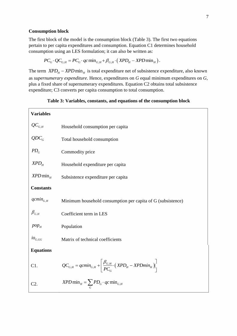
Consumption block

The first block of the model is the consumption block (Table 3). The first two equations

pertain to per capita expenditures and consumption. Equation C1 determines household

consumption using an LES formulation; it can also be written as:

, , ,min minG G H G G H G H H HPC QC PC qc XPD XPD .

The term minH HXPD XPD is total expenditure net of subsistence expenditure, also known

as supernumerary expenditure. Hence, expenditures on G equal minimum expenditures on G,

plus a fixed share of supernumerary expenditures. Equation C2 obtains total subsistence

expenditure; C3 converts per capita consumption to total consumption.

Table 3: Variables, constants, and equations of the consumption block

Variables

,G HQC Household consumption per capita

GQDC Total household consumption

GPD Commodity price

HXPD Household expenditure per capita

minHXPD Subsistence expenditure per capita

Constants

,G Hqcmin Minimum household consumption per capita of G (subsistence)

,G H Coefficient term in LES

Hpop Population

,G GGio Matrix of technical coefficients

Equations

C1. ,

, ,

G H

G H G H H H

G

QC qcmin XPD XPDminPC

C2. ,min minH G G H

G

XPD PD qc

8

C3. ,G G H H

H

QDC QC pop

To obtain constants ,G H and ,G Hqcmin , denote preliminary estimates of income and own

price elasticity as ,G H and ,G H , respectively; expenditure shares are denoted ,G Hw . The

following relations hold under the LES:

, , , ,; 1;G H G H G H G HG

w (1)

,

, ,

,

1 1G H

G H G H

G H

qcmin

QC . (2)

There is no guarantee however that the ,G H and ,G Hqcmin from (1) and (2) are consistent

with C2 and C1 at the baseline. Using GAMS Solver, the calibration entails imposition of

baseline data on C2 and C1 while minimizing the squared deviation of implied ,G H and ,G H

from initial estimates.

Household block

The second block of the model is the household block, shown in Table 4. Constants are all

calibrated from the SAM. Equation H1 sums up total factor income of households from the

value of labor endowment, adjusted by a parameter for entry into employment from

underemployed or surplus labor, assumed exogenous. H2 is the capital endowment of each

household; H3 obtains disposable income by netting out the direct income tax, while adding

transfers from government and rest of the world. H4, H5, and H6, simply derive,

respectively: the household income tax, household savings, and per capita household

expenditures.

Table 4: Variables, constants, and equations of the household block

Variables

HY Total household income

HKAPE Total household capital endowment

HYD Household disposable income per capita

SAV Total savings of households

YTAX Total tax on household income

PK Price of capital

PLA Price of agricultural labor

9

PLIS Price of industry-service labor

Constants

kapst Baseline capital stock

Hkapsh Ownership shares in capital stock

HAG Agricultural labor endowment per household per capita

HIS Labor endowment per household, industry-service, per capita

Entry into agricultural employment from underemployment

Hyt Direct tax rate on household

Hs Savings rate of household

Hgtranh Government transfers to households

Hftranh Foreign transfers to households (in USD)

Equations

H1. H H H H HY PKAP KAPE PLA AG pop PLIS IS

H2. H HKAPE kapsh kapst

H3. 1H H H H HYD Y yt gtranh ftranh

H4. H H

H

YTAX yt Y

H5. H H

H

SAV s YD

H6. 1H H

H

H

YD sXPD

pop

Production block

The third block is the production block, shown in Table 5. Value added is produced using

capital and labor by way of a constant elasticity of substitution (CES) function, with one

version for agricultural sectors (P1.1) and another for industry-service sectors (P1.2). The

10

specification adopts the Armington (1969) format. The elasticity of substitution GVA is

given by:

1

01

G

G

VAVA

; this implies 1

.GG

G

VAVA

VA

The price of value added

(ignoring first the subsidy term) is as follows:

;Ag Ag Ag Ag AgPVA PKAP KAP PLA LA ;

IS IS ISPVA PKAP LIS .

We obtain equations P2, P3, and P4, using cost-minimization on P1.1 and P1.2. In the

presence of a subsidy, the price of capital paid by the firm becomes 1 GPKAP sub , which

substitutes in P2.

Table 5: Variables, constants, and equations of the production block

Variables

GPVA Price of value added per good

GQVA Quantity of value added per good

GKAP Capital

AgLAG Agricultural labor

ISLIS Agricultural labor

GQS Domestic supply

GPS Price of domestic supply

VATAX Total domestic indirect tax

Constants

GKAP Capital parameter in CES value added (VA) function

AgLA Agricultural labor parameter in CES VA function

ISLIS Labor-services parameter in CES VA function

GVA Elasticity of substitution in CES VA function

11

GVA Parameter in CES VA function

Guva Value added per unit gross output

Gvat Implicit value added tax (net of subsidies)

Gsub Subsidy per unit capital (in ad valorem terms)

Equations

P1.1 1

Ag Ag AgVA VA VA

Ag Ag Ag Ag AgQVA KAP KAP LA LA

P1.2 1

IS IS ISVA VA VA

IS IS IS IS ISQVA KAP KAP LIS LIS

P2. 1

GVA

GG G G

G

PVAKAP QVA KAP

PKAP sub

P3. AgVA

GAg Ag Ag

PVALA QVA LA

PLA

P4. ISVA

ISIS IS IS

PVALIS QVA LIS

PLIS

P5. ,1G G G G GG G GG

GG

PS PVA vat uva io PD

P6. G G Guva QS QVA

P7. G G G

G

VATAX vat PVA QVA

Equation P5 obtains the price of gross output using value added plus the sum of intermediate

inputs per unit gross output, valued at the demand price. Value added, in quantity terms, is a

fixed share of gross output (P6). Lastly, the indirect domestic tax is assumed to be levied on

value added (P7).

Trade block

The third block is the trade block (Table 6). The domestically produced version of good G is

called the “home” good; the good demanded is a composite of home and imported goods,

based on the Armington (1969) formulation:

12

1

G G GD D D

G G G G GQD DH QDH DF QDF

.

From this we derive the conditional demands for the home good and the imported good,

respectively T1 and T2, with the elasticity of substitution obtained given by:

1

1G

G

DD

.

The domestically demanded version of good G is also called a home good; the good supplied

is a composite of is a composite of home and exported goods, based on the constant elasticity

of transformation (CET) function:

1

G G GS S S

G G G G GQS SH QSH SF QSF

From this we derive the conditional supplies for the home good and the exported good,

respectively T3 and T4, with the elasticity of transformation given by:

1

1G

G

SS

.

The price of the imported product is given in T5; the world price is converted to Philippine

peso using the exchange rate, taking into account an ad valorem tariff, and a further wedge

due to non-tariff barriers (also assumed to have an ad valorem effect). The counterpart for the

export price is T6, which far simpler in absence of export taxes and assuming away non-tariff

barriers on the supply side. The composite prices on demand side and supply side are given in

T7 and T8, respectively. T9 computes the total import taxes collected.

Table 6: Variables, constants, and equations of the trade block

Variables

GQD Total domestic demand (domestic absorption)

GQDH Demand for goods from home supplier

GQDF Import quantity (demand for goods from foreign supplier)

GQSH Supply of goods for home market

GQSF Export quantity (supply of goods for foreign buyer)

PUSD Price of USD in PHP (exchange rate)

GPM Border price of imported good

GPH Price of home supplied good for home market

13

GPX Border price of exported good

MTAX Total taxes on imports

Constants

Gpwm World price (in USD) of imported good

Gpwx World price (in USD) of exported good

Gtar Implicit tariff rate

GDH Coefficient in Armington composite for home source

GDF Coefficient in Armington composite for imports

GD Elasticity of substitution in Armington composite

GSH Coefficient in CET composite for home destination

GSF Coefficient in CET composite for foreign destination

GS Elasticity of transformation in CET composite

Gntb Non-tariff barrier effect on price

Equations

T1.

GD

G GG G

G

DH PDQDH QD

PH

T2.

GMD

GM GMGM GM

GM

DF PDQDF QD

PM

; 0GMNQdF

T3.

GS

GG G

G G

PHQSH QS

SH PS

T4.

GXS

GXGX GX

GX GX

PXQSF QS

SF PS

; 0GXNQSF .

T5. 1G G G GPM pwm PUSD tar ntb

14

T6. G GPX pwx PUSD

T7. G G G G G GPD QD PH QDH PM QDF

T8. G G G G G GPS QS PH QSH PX QSF

T9. G G G

G

MTAX tar pwm PUSD QDF

Other demand

The fourth block is the other demand block (Table 7). Total intermediate demand is the sum

of intermediate demands from the gross outputs based on the appropriate technical

coefficients (OD1). Expenditures on investment goods is a fixed share of total savings, based

on the capital allocation coefficient (OD2). Similarly, government consumption expenditures

is a fixed share of total government expenditures (OD3); note that total government

consumption is exogenous.

Table 7: Variables, constants, and equations of the other demand block

Variables

GQDINT Intermediate demand

GQDINV Investment demand

GQDGOV Government consumption demand

TSAV Total savings

Constants

Gcac Capital allocation coefficient

gxpd Total government consumption expenditure

G Shares in government consumption

ftrang Foreign transfers to government (in USD)

Equations

OD1. ,G G GG GG

GG

QDINT io QS

OD2. G G GPD QDINV cac TSAV

15

OD3. G G GPD QDGOV gxpd

OD4. G G G G GQD QDINT QDC QDINV QDGOV

Other institutions block

The fifth block is the other institutions block (Table 8). Government savings is total revenues

(taxes on income, business, and imports, together with transfers from foreign governments),

net of expenditures, total transfers to households, and subsidies (OI1). Foreign savings is

value of imports in pesos, net of import taxes, less value of exports, and transfers to

households and government from rest of the world (OI2); foreign savings is exogenous to the

model and posits the identity between base data foreign savings and normal capital inflows,

along with an open foreign exchange market. Imposition of (OI2) leads to the equilibrium

exchange rate. Total savings sums up savings of households, government, and rest of the

world (OI3).

Table 8: Variables, constants, and equations of the other institutions block

Variables

SAVG Savings of government (from consumption and income)

Constants

savf Savings of foreign

Equations

OI1. G G H G G

G H G

SAVG YTAX VATAX MTAX ftrang PUSD

PD QDGOV gtranh sub PKAP KAP

OI2.

1G G G

G

G G H

G H

savf pwm ntb PUSD QDF

PX QSF ftranh ftrang PUSD

OI3. TSAV SAV SAVG savf

Other closure block

The final block is the Other closure block (Table 9). Total demand for capital equals the total

stock of capital (OC1); likewise the total labor demand equals the total available labor (OC2

and OC3). The demand for domestically produced version of a good equals the domestically

supplied version of the good (OC4). Owing to non-uniqueness of the equilibrium price

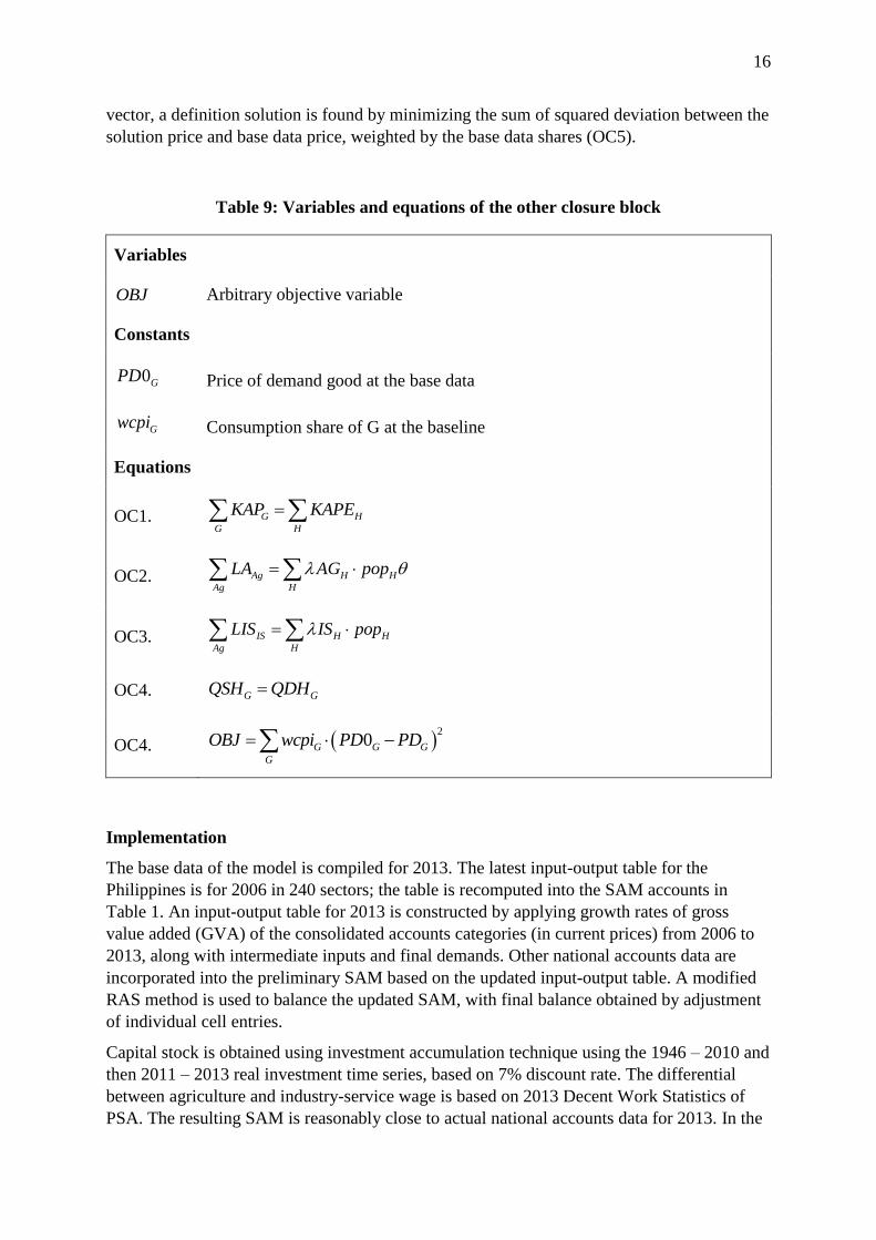
16

vector, a definition solution is found by minimizing the sum of squared deviation between the

solution price and base data price, weighted by the base data shares (OC5).

Table 9: Variables and equations of the other closure block

Variables

OBJ Arbitrary objective variable

Constants

0GPD Price of demand good at the base data

Gwcpi Consumption share of G at the baseline

Equations

OC1. G H

G H

KAP KAPE

OC2. Ag H H

Ag H

LA AG pop

OC3. IS H H

Ag H

LIS IS pop

OC4. G GQSH QDH

OC4. 2

0G G G

G

OBJ wcpi PD PD

Implementation

The base data of the model is compiled for 2013. The latest input-output table for the

Philippines is for 2006 in 240 sectors; the table is recomputed into the SAM accounts in

Table 1. An input-output table for 2013 is constructed by applying growth rates of gross

value added (GVA) of the consolidated accounts categories (in current prices) from 2006 to

2013, along with intermediate inputs and final demands. Other national accounts data are

incorporated into the preliminary SAM based on the updated input-output table. A modified

RAS method is used to balance the updated SAM, with final balance obtained by adjustment

of individual cell entries.

Capital stock is obtained using investment accumulation technique using the 1946 – 2010 and

then 2011 – 2013 real investment time series, based on 7% discount rate. The differential

between agriculture and industry-service wage is based on 2013 Decent Work Statistics of

PSA. The resulting SAM is reasonably close to actual national accounts data for 2013. In the

17

SAM, agriculture accounts for 11 percent of GDP, while agro-industry accounts for 21.2%.

Investment as a share in GDP is 20 percent. The capital stock is nearly double (196%) of

GDP, while the industry-service wage is 226% larger than the agriculture wage.

Calibration applies the usual method using initial estimates of expenditure elasticities, own-

price elasticities, and elasticities of substitution and transformation; Section 3 describes the

method for fine-tuning the elasticity estimates. Details of the code, compilation of the SAM,

and projections, are provided in a separate User’s Guide.

18

3. FRAMING THE SCENARIOS

Annual projections for the Philippine economy are computed from the base period to 2030,

the timeline set for the Sustainable Development Goals (SDGs). The scenarios are

distinguished by assumptions on productivity growth in the production of value added using a

shift term inserted as follows:

1

KAP LABQVA KAP LAB

.

This can be rewritten as:

1

1

KAP LABQVA KAP LAB

The elasticity of value added with respect to the shift term is given as follows:

% ln 1

.%

QVA QVA

Hence if there is a target percentage change in output due to technical progress, ceteris

paribus, then the following expression yields the required percentage change in the shift

parameter:

% % 1QVA

The scenarios to be analyzed are as follows:

Reference: identifying the productivity trends that will sustain the growth patterns

observed since 2010, which reflect targets set in the current PDP. Owing to slow

growth of agriculture over this period, this will likely entail weaker growth of

agricultural productivity relative to industry and services.

Productive agriculture: the same as Reference scenario, except productivity in

agriculture accelerates, to match that of industry and services.

Climate change: the same as Reference scenario, except agricultural productivity

remains flat owing to worsening impacts of climate change and other resource

constraints.

Productive industry-services: the same as Reference scenario, except productivity in

industry and services accelerates by half a percentage point per year.

Assumptions for productivity growth in the Reference scenario are aligned with recent

estimates in the literature, namely University of Groeningen and University of Davis (2017);

and Aba, Maglanoc, and Garoy (2015). Aside from the productivity growth projections,

replication of 2014 – 2016 data and expected trends in the Reference case is also used to tune

the parameters for: expenditure elasticity; own-price elasticity; elasticities of substitution and

transformation (production and trade blocks); and rate of depreciation of the capital stock.

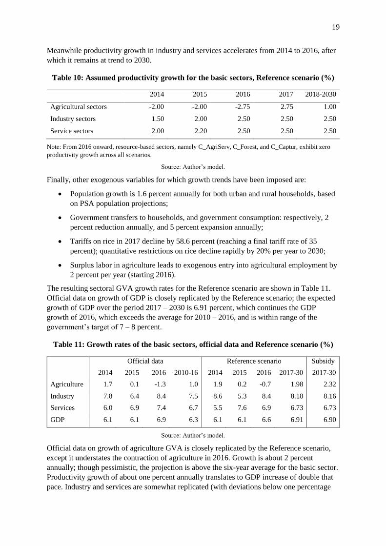
The assumed growth rates for the Reference scenario are shown in Table 10. Productivity

growth in agriculture is negative in 2014 – 2016 owing to climate shocks, intensified by the

El Nino of 2014-2015; in 2017, agriculture is expected to recover its productivity to at least

2015 level. However, trend growth in agricultural productivity is only one percent per annum.

19

Meanwhile productivity growth in industry and services accelerates from 2014 to 2016, after

which it remains at trend to 2030.

Table 10: Assumed productivity growth for the basic sectors, Reference scenario (%)

2014 2015 2016 2017 2018-2030

Agricultural sectors -2.00 -2.00 -2.75 2.75 1.00

Industry sectors 1.50 2.00 2.50 2.50 2.50

Service sectors 2.00 2.20 2.50 2.50 2.50

Note: From 2016 onward, resource-based sectors, namely C_AgriServ, C_Forest, and C_Captur, exhibit zero

productivity growth across all scenarios.

Source: Author’s model.

Finally, other exogenous variables for which growth trends have been imposed are:

Population growth is 1.6 percent annually for both urban and rural households, based

on PSA population projections;

Government transfers to households, and government consumption: respectively, 2

percent reduction annually, and 5 percent expansion annually;

Tariffs on rice in 2017 decline by 58.6 percent (reaching a final tariff rate of 35

percent); quantitative restrictions on rice decline rapidly by 20% per year to 2030;

Surplus labor in agriculture leads to exogenous entry into agricultural employment by

2 percent per year (starting 2016).

The resulting sectoral GVA growth rates for the Reference scenario are shown in Table 11.

Official data on growth of GDP is closely replicated by the Reference scenario; the expected

growth of GDP over the period 2017 – 2030 is 6.91 percent, which continues the GDP

growth of 2016, which exceeds the average for 2010 – 2016, and is within range of the

government’s target of 7 – 8 percent.

Table 11: Growth rates of the basic sectors, official data and Reference scenario (%)

Official data Reference scenario Subsidy

2014 2015 2016 2010-16 2014 2015 2016 2017-30 2017-30

Agriculture 1.7 0.1 -1.3 1.0 1.9 0.2 -0.7 1.98 2.32

Industry 7.8 6.4 8.4 7.5 8.6 5.3 8.4 8.18 8.16

Services 6.0 6.9 7.4 6.7 5.5 7.6 6.9 6.73 6.73

GDP 6.1 6.1 6.9 6.3 6.1 6.1 6.6 6.91 6.90

Source: Author’s model.

Official data on growth of agriculture GVA is closely replicated by the Reference scenario,

except it understates the contraction of agriculture in 2016. Growth is about 2 percent

annually; though pessimistic, the projection is above the six-year average for the basic sector.

Productivity growth of about one percent annually translates to GDP increase of double that

pace. Industry and services are somewhat replicated (with deviations below one percentage

20

point); expected growth in Industry GVA and Services GVA is 8.2 percent and 6.7 percent,

respectively. In contrast to agriculture, relatively modest productivity increases (less than 3

percent) drives a rapid pace of sector value added.

The Reference scenario incorporates a zero subsidy. To test the growth implications of a

subsidy on capital in agriculture, an alternative Reference scenario is posited with a capital

subsidy for agriculture equal to 5% off the cost of capital, except for rice, where the subsidy

is increased to 10% (in view of self-sufficiency targets). The subsidy is applied from 2018

onward.

The resulting growth rates are shown in the last column of Table 11. Growth of agriculture

accelerates moderately to 2.2 percent per year. Spending on subsidy begins at P47 billion in

2018, rising to P50 billion in 2030; these figures are within the range of annual budget

estimates of DA for subsidized credit during the Duterte administration.1

These expanded outlays slow down the rate of capital formation, hence the other sectors

suffer a mild growth slowdown. However, due to the far bigger share of these sectors in the

economy, overall GDP growth falls slightly. As expected, subsidies are of dubious value in

terms of promoting growth, and are set to zero in all of the scenarios.

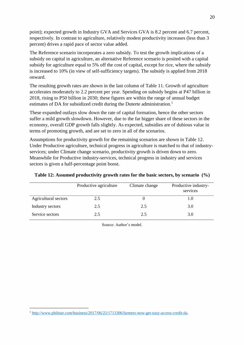
Assumptions for productivity growth for the remaining scenarios are shown in Table 12.

Under Productive agriculture, technical progress in agriculture is matched to that of industry-

services; under Climate change scenario, productivity growth is driven down to zero.

Meanwhile for Productive industry-services, technical progress in industry and services

sectors is given a half-percentage point boost.

Table 12: Assumed productivity growth rates for the basic sectors, by scenario (%)

Productive agriculture Climate change Productive industry-

services

Agricultural sectors 2.5 0 1.0

Industry sectors 2.5 2.5 3.0

Service sectors 2.5 2.5 3.0

Source: Author’s model.

1 http://www.philstar.com/business/2017/06/25/1713306/farmers-now-get-easy-access-credit-da.

21

4. RESULTS

Economywide growth

Official growth targets are achievable under trend rates of GDP growth.

Projections for GDP growth by scenario are shown in Figure 1. Given TFP growth rates

posited in Table 9, the reference scenario finds a TFP growth of about 7.5% initially, slowing

down slightly to 6.8% by 2030. This is somewhat below the 7-8% band, but well within the

neighborhood of the official growth target.

Figure 1: Scenarios for growth in GDP (%)

Source: Author’s model.

A small increment in TFP growth for industry-services leads to large increment in GDP

growth, contrasting with the impact of TFP growth in agriculture.

The economywide growth trajectory is largely unaffected by TFP trends in agriculture, even

by the climate change scenario. However, GDP growth is sharply elevated by faster TFP

growth in industry-services, peaking at 8.5% in 2017, but maintaining an 8.0 to 8.5% band

over the scenario horizon.

Agriculture

Overall growth in agriculture resembles the trend in agricultural TFP growth.

Extrapolating forward from TFP trends inferred from 2010 – 2016, weak growth in

agricultural GVA is attributable to low TFP growth. Hence if trend TFP growth continues, we

may expect agricultural GVA growth to remain in the 1 – 2 percent growth range.

Faster TFP growth in industry and services has no significant impact on the growth

trajectory of agriculture.

Somewhat surprisingly, changes in TFP growth trends in industry-services has no significant

impact on trends for agricultural growth. In fact, higher TFP growth in industry-services

slightly decreases that of agricultural GVA (about 0.20 percentage points) – due to re-

allocation of resources (labor and capital) from agriculture to industry-services.

22

Figure 2: Scenarios for growth in agricultural GVA (%)

Source: Author’s model.

Per capita consumption of primary agriculture will remain mostly unchanged over time,

though per capita consumption of processed food is expected to grow by 3-6% (except for

milled rice).

Growth in agricultural output similar to that of population growth of 1.6 percent (Figure 2).

This does not however imply deterioration in per capita consumption of food, even as high

income growth raises consumer purchasing power (Table 13).

Table 13: Growth in per capita consumption, by scenario (%)

Reference Agricultural

productivity

Climate change Industry-service

productivity

Rural Urban Rural Urban Rural Urban Rural Urban

C_Corn 0.04 0.04 0.05 0.05 0.03 0.03 0.05 0.05

C_Coconut 0.02 0.02 0.04 0.04 0.01 0.01 0.03 0.02

C_Sugarcane 0.00 0.00 0.00 0.00 0.00 0.00 0.00 0.00

C_Banana -0.03 -0.03 -0.01 -0.01 -0.03 -0.04 -0.03 -0.04

C_Mango 0.01 0.01 0.04 0.03 0.00 0.00 0.02 0.01

C_Otfruit 0.04 0.04 0.05 0.05 0.04 0.04 0.06 0.05

C_Otcrop 0.06 0.06 0.06 0.06 0.06 0.06 0.08 0.08

C_Rootcrop 0.02 0.01 0.04 0.04 0.01 0.00 0.02 0.01

C_Veg 0.02 0.01 0.04 0.03 0.01 0.00 0.02 0.01

C_Aquacult 0.02 0.02 0.04 0.04 0.01 0.01 0.03 0.02

C_Mining 0.08 0.08 0.08 0.08 0.08 0.08 0.10 0.10

C_Rice 0.73 0.74 0.78 0.79 0.70 0.71 0.90 0.90

C_Meat 3.60 3.52 4.23 4.17 3.23 3.15 4.18 4.12

C_Procfish 3.25 3.15 3.50 3.39 3.11 3.03 3.97 3.89

C_Sugar 3.52 3.44 4.07 4.00 3.26 3.19 4.18 4.12

C_Otfoodmanuf 4.40 4.38 4.78 4.75 4.17 4.15 5.12 5.11

C_Bev 4.91 4.92 5.08 5.07 4.80 4.83 5.75 5.76

Source: Author’s model.

23

The table makes clear though that the most rapid rates of consumption growth are not for

primary agricultural products, but rather for processed agricultural products, other

manufacturing, and services. This reflects the imposition of income inelastic demand for

primary products, and elasticities at unity or higher for processed food, manufactured

products, and services.

Industry, service, and agro-industry

Industry will lead in growth performance, with service remaining at average pace. Both

sectors largely unaffected by changes in agricultural productivity.

Growth of industry begins at an outstanding 9 percent clip in 2017, but tapering off to around

8 percent average pace in 2025 onward (Figure 3). Meanwhile, growth of services begins at 7

percent, and adjusts slightly down to 6.5 percent in 2030. The trends are mostly unchanged

whether there is an acceleration or deceleration of productivity growth in agriculture.

Figure 3: Scenarios for growth in industry GVA (%)

Source: Author’s model.

Figure 4: Scenarios for growth in service GVA (%)

Source: Author’s model.

Growth in industry-service GVA rises significantly with small increment in productivity

growth.

With just a 0.5 percentage point addition in TFP growth, growth of industry GVA rises

sharply to 11 percent by 2019, and staying at above 9.5 percent by 2030. Similarly, growth of

24

service GVA accelerates to nearly 8.5 percent, before falling off to about 7.5 percent by

2030.

Acceleration in agricultural TFP growth has only modest impact on agri-related industry

growth, compared to accelerated I-S TFP growth.

Under the Reference scenario, the growth rate of agri-related industry GVA averages only

3.52 percent, far slower than the pace of overall industry growth. Beginning from over 6

percent growth in 2017, the industry cluster slows down to just about 3 percent growth in

2019, slightly accelerating to 3.62 percent by 2030 (Figure 5). The share of agri-related

industry in GDP is 8.6 percent in 2016, falling to just 4.3 percent in 2030.

Faster productivity growth of agriculture likewise boosts growth of agri-related industry,

stabilizing its growth pace at about 5 percent per year. On the other hand, adverse climate

change depresses agri-related industry growth down to about 2 percent. There is no sharp

change in trajectory with faster industry-service growth, compared to the Reference scenario;

though the trajectories begin to diverge at around 2027, when growth rates under the

Productive-industry services scenario become noticeable faster.

Figure 5: Scenarios for growth in agri-related industry GVA (%)

Source: Author’s model.

Wages

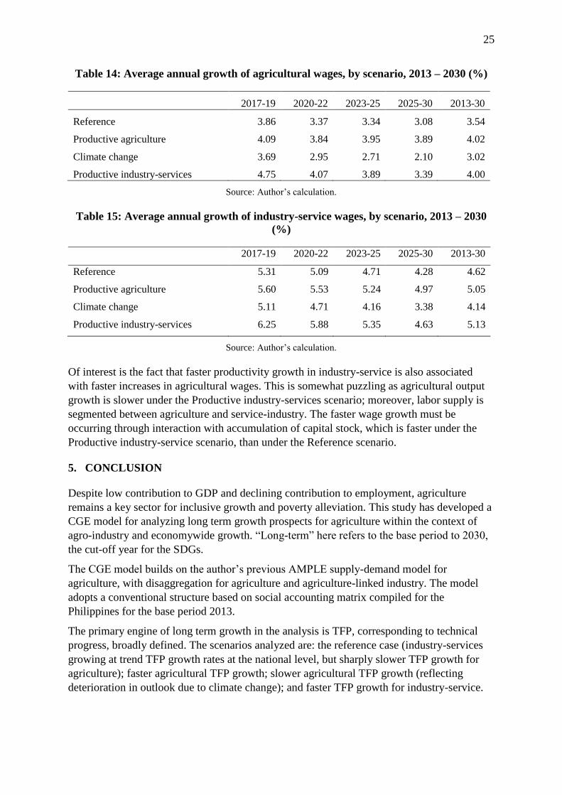
Agricultural wages will grow, but will be outpaced by industry-service wages.

Projections for wages are shown in Table 14 and 15. Growth starts at above 4 percent

annually, slowing down to 3 percent by 2030; however, that of industry-service ranges from 4

to 5 percent. Over time therefore wages of agriculture and industry-service will continue to

diverge.

Growth in agricultural wage is significantly affected by productivity growth in agriculture, as

well as by productivity growth in industry-service.

The wage projection for industry-service is mostly unaffected by changes in agricultural

productivity; it is only significantly affected by faster productivity growth in industry-service

itself. Likewise, agricultural wages are positively and significantly affected by productivity

growth in agriculture.

25

Table 14: Average annual growth of agricultural wages, by scenario, 2013 – 2030 (%)

2017-19 2020-22 2023-25 2025-30 2013-30

Reference 3.86 3.37 3.34 3.08 3.54

Productive agriculture 4.09 3.84 3.95 3.89 4.02

Climate change 3.69 2.95 2.71 2.10 3.02

Productive industry-services 4.75 4.07 3.89 3.39 4.00

Source: Author’s calculation.

Table 15: Average annual growth of industry-service wages, by scenario, 2013 – 2030

(%)

2017-19 2020-22 2023-25 2025-30 2013-30

Reference 5.31 5.09 4.71 4.28 4.62

Productive agriculture 5.60 5.53 5.24 4.97 5.05

Climate change 5.11 4.71 4.16 3.38 4.14

Productive industry-services 6.25 5.88 5.35 4.63 5.13

Source: Author’s calculation.

Of interest is the fact that faster productivity growth in industry-service is also associated

with faster increases in agricultural wages. This is somewhat puzzling as agricultural output

growth is slower under the Productive industry-services scenario; moreover, labor supply is

segmented between agriculture and service-industry. The faster wage growth must be

occurring through interaction with accumulation of capital stock, which is faster under the

Productive industry-service scenario, than under the Reference scenario.

5. CONCLUSION

Despite low contribution to GDP and declining contribution to employment, agriculture

remains a key sector for inclusive growth and poverty alleviation. This study has developed a

CGE model for analyzing long term growth prospects for agriculture within the context of

agro-industry and economywide growth. “Long-term” here refers to the base period to 2030,

the cut-off year for the SDGs.

The CGE model builds on the author’s previous AMPLE supply-demand model for

agriculture, with disaggregation for agriculture and agriculture-linked industry. The model

adopts a conventional structure based on social accounting matrix compiled for the

Philippines for the base period 2013.

The primary engine of long term growth in the analysis is TFP, corresponding to technical

progress, broadly defined. The scenarios analyzed are: the reference case (industry-services

growing at trend TFP growth rates at the national level, but sharply slower TFP growth for

agriculture); faster agricultural TFP growth; slower agricultural TFP growth (reflecting

deterioration in outlook due to climate change); and faster TFP growth for industry-service.

26

One key finding is that subsidies on capital in agriculture (the current policy thrust of

Department of Agriculture) slightly accelerates growth of agriculture, but acts as a drag on

overall growth by slowing down the rate of capital formation. On the other hand, maintaining

productivity growth for industry-services, trend rates suffices to reach PDP growth targets,

despite weak TFP growth for agriculture.

As for agriculture, the scenario analysis finds that weak growth performance of agriculture

will persist as long as TFP performance does. From the perspective of food security, this does

not mean that per capita food consumption will necessarily fall; however, implications for

livelihoods and the pace of poverty reduction are unclear, requiring further analysis and

development of an equity-sensitive version of AMPLE-CGE. One clue is that agricultural

wages are projected rise, but wage disparity vis-à-vis industry-service continues to widen

over time.

Meanwhile, varying the rate of TFP growth in agriculture impacts strongly on agriculture

itself, but hardly affects growth prospects of the industry-service sectors. Conversely, TFP

growth in the latter strongly on itself and overall GDP, but not on agriculture. In short, the

scenario analysis finds little support for strong indirect impacts, except for agricultural wages

being affected by industry-service growth.

The analysis spotlights the necessity of boosting productivity growth, as opposed to devoting

resources towards artificially increasing returns to investments, even in a key sector such as

agriculture. Going into the specifics of TFP growth enhance is beyond the scope of this

paper; it suffices to say that TFP is generally not increased by price support policies for

agriculture, nor by subsidies on private goods, contrary to the current thrust of agricultural

policy. Elements for accelerating TFP growth are instead: R&D, innovation, adoption of

technology, improved practices and systems, public goods (e.g. transport infrastructure).

If the goal is sustaining rapid, economywide growth, the analysis emphasizes industry-service

TFP over that of agriculture. Further research is needed to establish whether equity

considerations will justify great focus on agriculture TFP.

Furthermore, the lack of indirect impact from agriculture to industry-service, and vice-versa,

seems to invalidate the value chain strategy to agriculture advocated in the latest incarnation

of the PDP. However, such a conclusion is premature. The value chain strategy aims at

stronger integration between agriculture and industry-service, as well as encouraging agro-

industry-specific capital formation. For as long as these subsidies for private goods are

avoided, and more cost-effective mechanisms pursued, e.g. cluster-based approach,

establishing agricultural value chains may yet be a viable strategy for inclusive growth.

27

REFERENCES

Aba, P., D. Maglanoc, and E. Garoy. 2016. Measuring Growth Residual: Empirical Evidence

on Total Factor Productivity Test and Solow Growth Model. Paper presented at the 13th

National Convention on Statistics, Mandaluyong City.

Armington, P. 1969. A theory of demand for products distinguished by place of production.

IMF Staff Papers 16(1): 159 – 78.

Briones, R., 2014. Scenarios and options for Philippine agriculture. In: Briones, R., M.A.

Sombilla, and A. Balisacan, eds. Productivity Growth in Philippine Agriculture. SEARCA,

Department of Agriculture – Bureau of Agricultural Research, and Philippine Rice Research

Institute, Los Baños, Laguna, Philippines.

Briones, R. 2016. Growing inclusive businesses in the Philippines: the role of government

policies and programs. Discussion Paper Series No. 2016-06. PIDS, Quezon City.

Dervis, K., J. de Melo, S. Robinson. 1982. General Equilibrium Models for Development.

World Bank, Washington, D.C.

Lofgren, H., R. Harris, S. Robinson. 2002. A standard computable general equilibrium (CGE)

model in GAMS. Microcomputers in Policy Research No. 5. International Food Policy

Research Institute, Washington, D.C.

NEDA [National Economic Development Authority]. 2017. The Philippine Development

Plan 2017 – 2022. NEDA, Pasig City, Philippines.

Robichaud, V., A. Lemelin, H. Maisonnave, B. Decaluwe. 2012. PEP-1-1 A User Guide.

Poverty and Economic Policy Network, Quebec. https://www.pep-net.org/pep-standard-cge-

models. Accessed 30 December 2016.

University of Groningen and University of California, Davis, Total Factor Productivity at

Constant National Prices for Philippines [RTFPNAPHA632NRUG], retrieved from FRED,

Federal Reserve Bank of St. Louis Https://fred.stlouisfed.org/series/RTFPNAPHA632NRUG.

Accessed July 10, 2017.