Outline - Uppsala Universityuser.it.uu.se/~thosc112/CLDS_UTFSM/lecture3handout.… · · 2014-01-20density p ( x t j y: t). lters 2014. Outline 3(44) 1.2 2.xample 3.methods a)sampling

Lecture 3 - Particle filters

Thomas Schöne-mail: [email protected]

Division of Systems and ControlDepartment of Information TechnologyUppsala University

Lecture 3 - Particle filtersThomas Schön, Summer School at Universidad Técnica Federico Santa María, Valparaíso, Chile in January 2014.

The aim – Lecture 3 2(44)

The aim in Lecture 3 is to introduce the particle filter.

This will be done by first explaining some key sampling strategies.

We then derive a first working particle filter by setting up animportance sampler targeting the filtering density p(xt | y1:t).


Outline 3(44)

1. Summary of lecture 2

2. Particle filter – introductory example3. Basic sampling methods

a) Rejection samplingb) Importance sampling

4. Application example – indoor positioning

5. A first working particle filter

6. A particle filter targeting the JSD

7. The particle degeneracy problem

8. Application example – UAV positioning


Summary – Lecture 2 (I/II) 4(44)

The goal in maximum likelihood is to find the θ that best describesthe distribution from which the data comes from.

θML

= arg maxθ∈Θ

∫. . .∫

µθ(x1)T

∏t=1

gθ(yt | xt)T

∏t=1

pθ(xt | y1:t−1)dx1:T

The expectation maximization (EM) algorithm computes maximumlikelihood estimates of unknown parameters in probabilistic modelsinvolving latent variables.


Summary – Lecture 2 (II/II) 5(44)

The goal in Bayesian modeling is to compute the posteriorp(θ, x1:T | y1:T) = p(η | y1:T) (or one of its marginals).

p(η | y1:T) =

likelihood︷︸︸︷p(y1:T | η)

prior︷︸︸︷p(η)

p(y1:T)︸︷︷︸marginal likelihood

Markov chain Monte Carlo (MCMC) methods allows us to generatesamples from a target density π(z) by simulating a Markov chain.Constructive algorithms:

1. Metropolis Hastings sampler

2. Gibbs sampler


Particle filter – introductory example (I/III) 6(44)

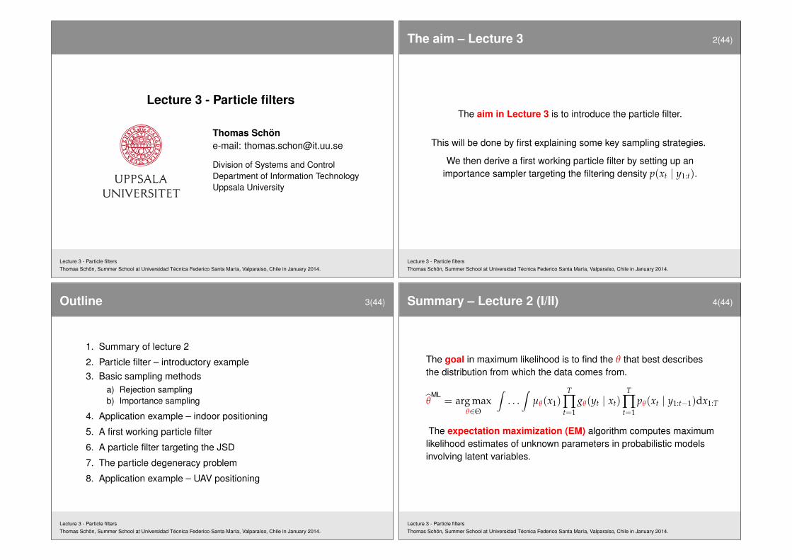
Consider a toy 1D localization problem.

0 20 40 60 80 1000

10

20

30

40

50

60

70

80

90

100

110

Posit ion x

Altitude

Dynamic model:

xt+1 = xt + ut + vt,

where xt denotes position, ut denotes velocity(known), vt ∼ N (0, 5) denotes an unknowndisturbance.

Measurements:

yt = h(xt) + et.

where h(·) denotes the world model (here theterrain height) and et ∼ N (0, 1) denotes anunknown disturbance.


Particle filter – introductory example (II/III) 7(44)

Task: Find the state xt based on a set of measurementsy1:t , {y1, . . . , yt}. Do this by computing the filter PDF p(xt | y1:t).

The particle filter maintains an approximation according to

p(xt | y1:t) =N

∑i=1

witδxi

t(xt),

where each sample xit is referred to as a particle.

For intuition: Think of each particle as one simulation of the systemstate (in this example the horizontal position) and only keep the goodones.


Particle filter – introductory example (III/III) 8(44)

Highlights two keycapabilities of the PF:

1. Automaticallyhandles an unknownand dynamicallychanging number ofhypotheses.

2. Work withnonlinear/non-Gaussianmodels.


Rejection sampling (I/VII) 9(44)

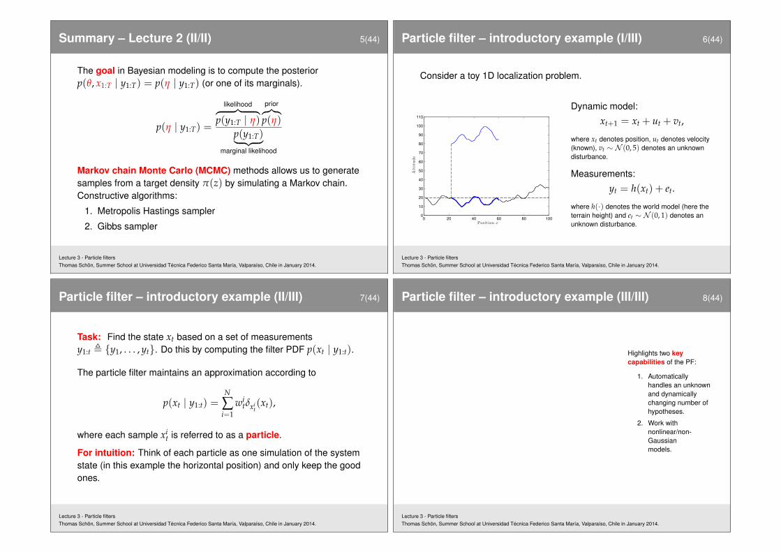
Rejection sampling is a Monte Carlo method that produce i.i.d.samples from a target distribution

π(z) =π(z)Cπ

,

where π(z) can be evaluated and Cπ is a normalization constant.

Key idea: Generate randomnumbers uniformly from the areaunder the graph of the targetdistribution π(z).

Just as hard as the originalproblem, but what if...


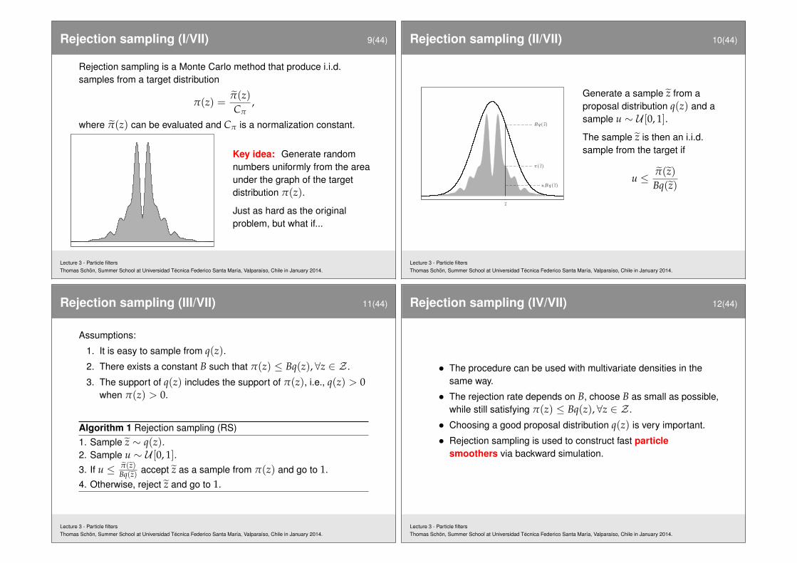
Rejection sampling (II/VII) 10(44)

z

π( z)

Bq ( z)

uBq ( z)

Generate a sample z from aproposal distribution q(z) and asample u ∼ U [0, 1].

The sample z is then an i.i.d.sample from the target if

u ≤ π(z)Bq(z)


Rejection sampling (III/VII) 11(44)

Assumptions:

1. It is easy to sample from q(z).2. There exists a constant B such that π(z) ≤ Bq(z), ∀z ∈ Z .

3. The support of q(z) includes the support of π(z), i.e., q(z) > 0when π(z) > 0.

Algorithm 1 Rejection sampling (RS)1. Sample z ∼ q(z).2. Sample u ∼ U [0, 1].3. If u ≤ π(z)

Bq(z) accept z as a sample from π(z) and go to 1.

4. Otherwise, reject z and go to 1.


Rejection sampling (IV/VII) 12(44)

• The procedure can be used with multivariate densities in thesame way.

• The rejection rate depends on B, choose B as small as possible,while still satisfying π(z) ≤ Bq(z), ∀z ∈ Z .

• Choosing a good proposal distribution q(z) is very important.

• Rejection sampling is used to construct fast particlesmoothers via backward simulation.


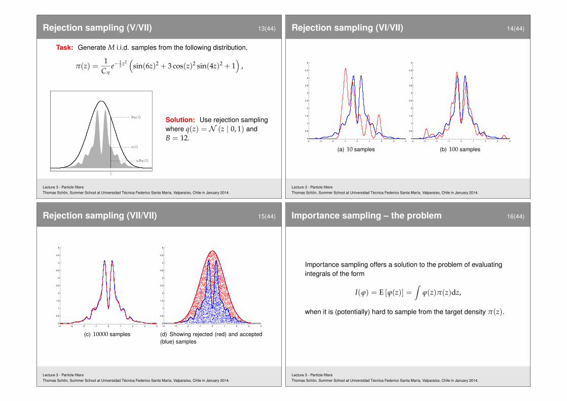
Rejection sampling (V/VII) 13(44)

Task: Generate M i.i.d. samples from the following distribution,

π(z) =1

Cπe−

12 z2(

sin(6z)2 + 3 cos(z)2 sin(4z)2 + 1)

,

z

π( z)

Bq ( z)

uBq ( z)

Solution: Use rejection samplingwhere q(z) = N (z | 0, 1) andB = 12.


Rejection sampling (VI/VII) 14(44)

−4 −3 −2 −1 0 1 2 3 4

0

0.5

1

1.5

2

2.5

3

3.5

4

4.5

5

(a) 10 samples

−4 −3 −2 −1 0 1 2 3 4

0

0.5

1

1.5

2

2.5

3

3.5

4

4.5

5

(b) 100 samples


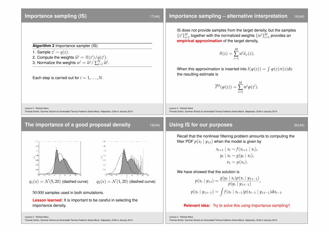
Rejection sampling (VII/VII) 15(44)

−4 −3 −2 −1 0 1 2 3 4

0

0.5

1

1.5

2

2.5

3

3.5

4

4.5

5

(c) 10000 samples

−4 −3 −2 −1 0 1 2 3 4

0

0.5

1

1.5

2

2.5

3

3.5

4

4.5

5

(d) Showing rejected (red) and accepted(blue) samples


Importance sampling – the problem 16(44)

Importance sampling offers a solution to the problem of evaluatingintegrals of the form

I(ϕ) = E [ϕ(z)] =∫

ϕ(z)π(z)dz,

when it is (potentially) hard to sample from the target density π(z).


Importance sampling (IS) 17(44)

Algorithm 2 Importance sampler (IS)

1. Sample zi ∼ q(z).2. Compute the weights wi = π(zi)/q(zi).3. Normalize the weights wi = wi/ ∑N

j=1 wj.

Each step is carried out for i = 1, . . . , N.


Importance sampling – alternative interpretation 18(44)

IS does not provide samples from the target density, but the samples{zi}M

i=1 together with the normalized weights {wi}Mi=1 provides an

empirical approximation of the target density,

π(z) =M

∑i=1

wiδzi(z).

When this approximation is inserted into I(ϕ(z)) =∫

ϕ(z)π(z)dzthe resulting estimate is

IM(ϕ(z)) =M

∑i=1

wi ϕ(zi).


The importance of a good proposal density 19(44)

q1(x) = N (5, 20) (dashed curve) q2(x) = N (1, 20) (dashed curve)

50 000 samples used in both simulations.

Lesson learned: It is important to be careful in selecting theimportance density.


Using IS for our purposes 20(44)

Recall that the nonlinear filtering problem amounts to computing thefilter PDF p(xt | y1:t) when the model is given by

xt+1 | xt ∼ f (xt+1 | xt),yt | xt ∼ g(yt | xt),

x1 ∼ µ(x1).

We have showed that the solution is

p(xt | y1:t) =g(yt | xt)p(xt | y1:t−1)

p(yt | y1:t−1),

p(xt | y1:t−1) =∫

f (xt | xt−1)p(xt−1 | y1:t−1)dxt−1.

Relevant idea: Try to solve this using importance sampling!!


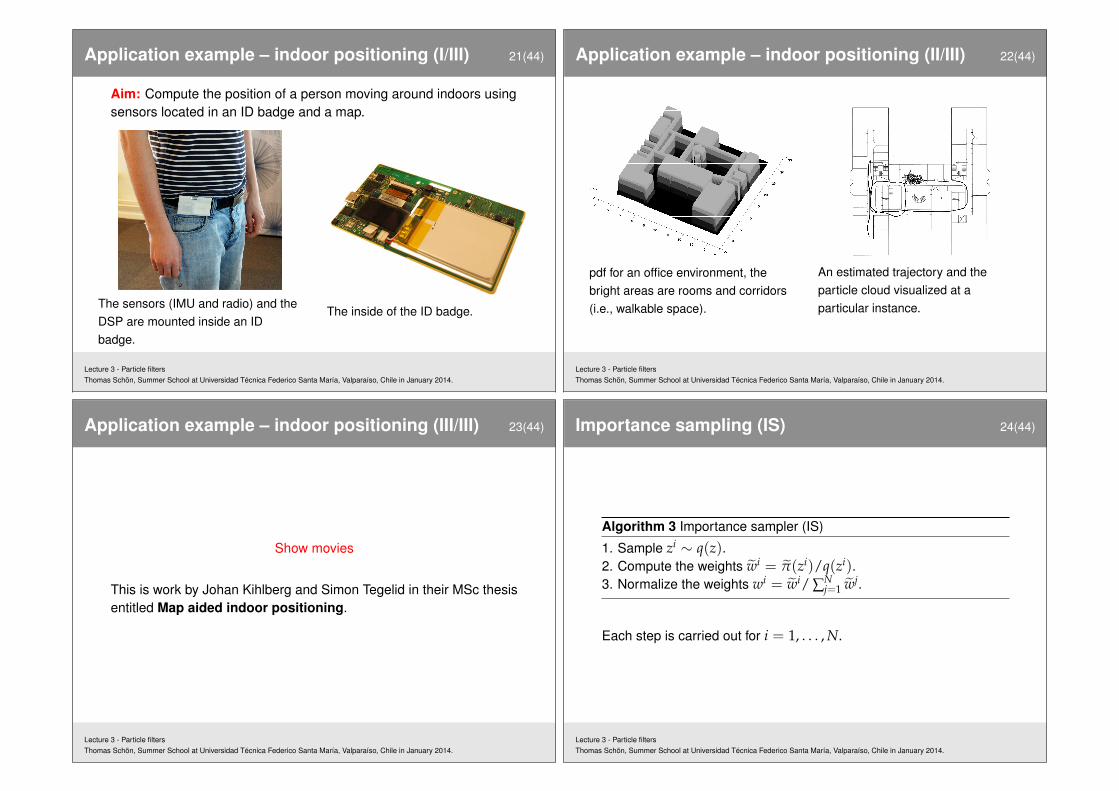
Application example – indoor positioning (I/III) 21(44)

Aim: Compute the position of a person moving around indoors usingsensors located in an ID badge and a map.

1.5 Xdin 3

(a) A Beebadge, carrying a numberof sensors and a IEEE 802.15.4 radiochip.

(b) A coordinator, equipped bothwith a radio chip and an Ethernetport, serving as a base station for theBeebadges.

Figure 1.1. The two main components of the radio network.

Figure 1.2. Beebadge worn by a man.The sensors (IMU and radio) and theDSP are mounted inside an IDbadge.

1.5 Xdin 3

(a) A Beebadge, carrying a numberof sensors and a IEEE 802.15.4 radiochip.

(b) A coordinator, equipped bothwith a radio chip and an Ethernetport, serving as a base station for theBeebadges.

Figure 1.1. The two main components of the radio network.

Figure 1.2. Beebadge worn by a man.

The inside of the ID badge.


Application example – indoor positioning (II/III) 22(44)2.5 Map 15

(a) Relative probability density for parts ofXdin’s o�ce, the bright areas are rooms andthe bright lines are corridors that interconnectthe rooms

!1.5 !1 !0.5 0 0.5 1 1.50

0.2

0.4

0.6

0.8

1

Position [m]

Re

lativ

e p

rob

ab

ility

Decay for different n

n=2, m=1n=3, m=1n=4, m=1

(b) Cross section of the relative prob-ability function for a line with di�er-ent n

Figure 2.7. Probability interpretation of the map.

those would su�ce to give a magnitude of the force. The force is intuitivelydirected orthogonally from the wall towards the target and multiple forces canbe added together to get a resulting force a�ecting the momentum of the target.

Equation (2.9) describes how the force is constructed. The function wallj(p)is a convex function giving the magnitude and direction of the force given theposition of the target, p.

fi =ÿ

jœWwallj(pi), where W is the set of walls. (2.9)

If positions from other targets are available, repellent forces from them can bemodeled as well, which is thoroughly discussed in [22]. The concept is visualizedin Figure 2.8 where the target Ti is a�ected by two walls and another targetTm, resulting in the force fi.

Figure 2.8. Force vectors illustrating the resulting force a�ecting a pedestrian.

pdf for an office environment, thebright areas are rooms and corridors(i.e., walkable space).

48 Approach

(a) An estimated trajectory at Xdin’s of-fice, 1000 particles represented as circles,size of a circle indicates the weight of theparticle.

(b) A scenario where the filter have notconverged yet. The spread in hypothesesis caused by a large coverage for a coordi-nator.

Figure 4.10. Output from the particle filter.

Figure 4.11. Illustration of a problematic case where a correct trajectory (green) isbeing starved by an incorrect trajectory (red), causing the filter to potentially diverge.

An estimated trajectory and theparticle cloud visualized at aparticular instance.


Application example – indoor positioning (III/III) 23(44)

Show movies

This is work by Johan Kihlberg and Simon Tegelid in their MSc thesisentitled Map aided indoor positioning.


Importance sampling (IS) 24(44)

Algorithm 3 Importance sampler (IS)

1. Sample zi ∼ q(z).2. Compute the weights wi = π(zi)/q(zi).3. Normalize the weights wi = wi/ ∑N

j=1 wj.

Each step is carried out for i = 1, . . . , N.


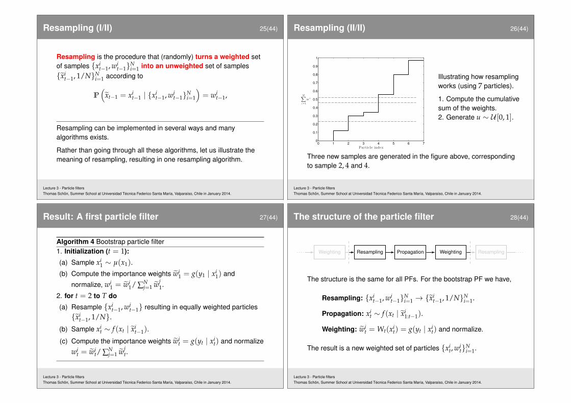
Resampling (I/II) 25(44)

Resampling is the procedure that (randomly) turns a weighted setof samples {xi

t−1, wit−1}N

i=1 into an unweighted set of samples{xi

t−1, 1/N}Ni=1 according to

P(

xt−1 = xit−1 | {xi

t−1, wit−1}N

i=1

)= wi

t−1,

Resampling can be implemented in several ways and manyalgorithms exists.

Rather than going through all these algorithms, let us illustrate themeaning of resampling, resulting in one resampling algorithm.


Resampling (II/II) 26(44)

0 1 2 3 4 5 6 70

0.1

0.2

0.3

0.4

0.5

0.6

0.7

0.8

0.9

1

M∑

i=1

wi

Partic le index

Illustrating how resamplingworks (using 7 particles).

1. Compute the cumulativesum of the weights.2. Generate u ∼ U [0, 1].

Three new samples are generated in the figure above, correspondingto sample 2, 4 and 4.


Result: A first particle filter 27(44)

Algorithm 4 Bootstrap particle filter1. Initialization (t = 1):

(a) Sample xi1 ∼ µ(x1).

(b) Compute the importance weights wi1 = g(y1 | xi

1) and

normalize, wi1 = wi

1/ ∑Nj=1 wj

1.

2. for t = 2 to T do

(a) Resample {xit−1, wi

t−1} resulting in equally weighted particles{xi

t−1, 1/N}.(b) Sample xi

t ∼ f (xt | xit−1).

(c) Compute the importance weights wit = g(yt | xi

t) and normalize

wit = wi

t/ ∑Nj=1 wj

t.


The structure of the particle filter 28(44)

The structure is the same for all PFs. For the bootstrap PF we have,

Resampling: {xit−1, wi

t−1}Ni=1 → {xi

t−1, 1/N}Ni=1.

Propagation: xit ∼ f (xt | xi

1:t−1).

Weighting: wit = Wt(xi

t) = g(yt | xit) and normalize.

The result is a new weighted set of particles {xit, wi

t}Ni=1.


Weighting Resampling Propagation Weighting Resampling

An LGSS example (I/II) 29(44)

“Whenever you are working on a nonlinear inference method,always make sure that it solves the linear special case first.”

Consider the following LGSS model (simple one dimensionalpositioning example)

pt+1vt+1at+1

=

1 Ts T2s /2

0 1 Ts0 0 1

ptvtat

+

(T3

s /6T2

s /2Ts

)vt, vt ∼ N (0, Q),

yt =

(1 0 00 0 1

)

ptvtat

+ et, et ∼ N (0, R).

The KF provides the true filtering density, which implies that we cancompare the PF to the truth in this case.


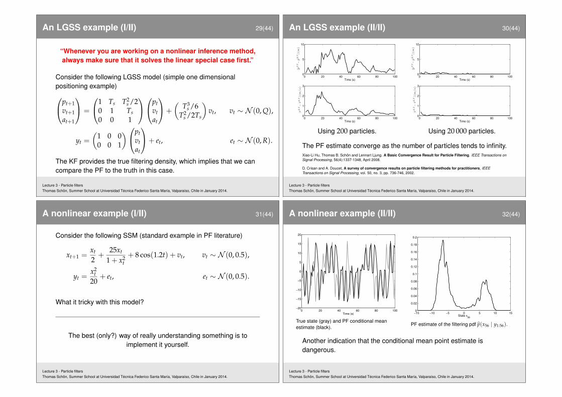
An LGSS example (II/II) 30(44)

0 20 40 60 80 1000

5

10

Time (s)

|pPF−

pK

F|(m

)

0 20 40 60 80 1000

1

2

3

Time (s)

|vK

F−

vK

F|(m

/s)

Using 200 particles.

0 20 40 60 80 1000

5

10

Time (s)

|pPF−

pK

F|(m

)

0 20 40 60 80 1000

1

2

3

Time (s)

|vK

F−

vK

F|(m

/s)

Using 20 000 particles.

The PF estimate converge as the number of particles tends to infinity.Xiao-Li Hu, Thomas B. Schön and Lennart Ljung. A Basic Convergence Result for Particle Filtering. IEEE Transactions onSignal Processing, 56(4):1337-1348, April 2008.

D. Crisan and A. Doucet, A survey of convergence results on particle filtering methods for practitioners, IEEETransactions on Signal Processing, vol. 50, no. 3, pp. 736-746, 2002.


A nonlinear example (I/II) 31(44)

Consider the following SSM (standard example in PF literature)

xt+1 =xt

2+

25xt

1 + x2t+ 8 cos(1.2t) + vt, vt ∼ N (0, 0.5),

yt =x2

t20

+ et, et ∼ N (0, 0.5).

What it tricky with this model?

The best (only?) way of really understanding something is toimplement it yourself.


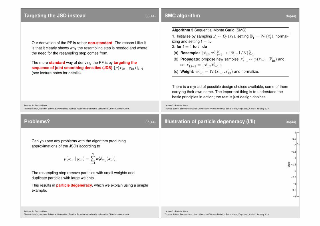
A nonlinear example (II/II) 32(44)

0 20 40 60 80 100−20

−15

−10

−5

0

5

10

15

20

Time (s)

True state (gray) and PF conditional meanestimate (black).

−15 −10 −5 0 5 10 150

0.02

0.04

0.06

0.08

0.1

0.12

0.14

0.16

0.18

0.2

State x56

PF estimate of the filtering pdf p(x56 | y1:56).

Another indication that the conditional mean point estimate isdangerous.


Targeting the JSD instead 33(44)

Our derivation of the PF is rather non-standard. The reason I like itis that it clearly shows why the resampling step is needed and wherethe need for the resampling step comes from.

The more standard way of deriving the PF is by targeting thesequence of joint smoothing densities (JDS) {p(x1:t | y1:t)}t≥1(see lecture notes for details).


SMC algorithm 34(44)

Algorithm 5 Sequential Monte Carlo (SMC)

1. Initialise by sampling xi1 ∼ Q1(x1), setting wi

1 = W1(xi1), normal-

izing and setting t = 1.2. for t = 1 to T do

(a) Resample: {xi1:t, wi

t}Ni=1 → {xi

1:t, 1/N}Ni=1.

(b) Propagate: propose new samples, xit+1 ∼ qt(xt+1 | xi

1:t) andset xi

1:t+1 = {xi1:t, xi

t+1}.(c) Weight: wi

t+1 = Wt(xit+1, xi

1:t) and normalize.

There is a myriad of possible design choices available, some of themcarrying their own name. The important thing is to understand thebasic principles in action; the rest is just design choices.


Problems? 35(44)

Can you see any problems with the algorithm producingapproximations of the JSDs according to

p(x1:t | y1:t) =N

∑i=1

witδxi

1:t(x1:t)

The resampling step remove particles with small weights andduplicate particles with large weights.

This results in particle degeneracy, which we explain using a simpleexample.


Illustration of particle degeneracy (I/II) 36(44)

5 10 15 20 25−4

−3.5

−3

−2.5

−2

−1.5

−1

−0.5

0

0.5

1

Time

Sta

te


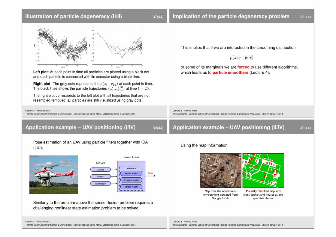
Illustration of particle degeneracy (II/II) 37(44)

5 10 15 20 25−4

−3.5

−3

−2.5

−2

−1.5

−1

−0.5

0

0.5

1

Time

Sta

te

5 10 15 20 25−4

−3.5

−3

−2.5

−2

−1.5

−1

−0.5

0

0.5

1

Time

Sta

te

Left plot: At each point in time all particles are plotted using a black dotand each particle is connected with its ancestor using a black line.

Right plot: The grey dots represents the p(xt | y1:t) at each point in time.The black lines shows the particle trajectories {xi

1:25}30i=1 at time t = 25.

The right plot corresponds to the left plot with all trajectories that are notresampled removed (all particles are still visualized using gray dots).


Implication of the particle degeneracy problem 38(44)

This implies that if we are interested in the smoothing distribution

p(x1:T | y1:T)

or some of its marginals we are forced to use different algorithms,which leads us to particle smoothers (Lecture 4).


Application example – UAV positioning (I/IV) 39(44)

Pose estimation of an UAV using particle filters together with IDA(LiU).

Sensor fusion in dynamical systemsThomas Schön, users.isy.liu.se/rt/schon

SIGRAD 2013Norrköping, Sweden

2. Helicopter pose estimation using a map (I/III)

Aim: Compute the position and orientation of a helicopter by exploiting the information present in Google maps images of the operational area.

World model

Inference

Dynamic model

Sensor model

Sensors

Sensor fusion

PoseCamera

Inertial

Barometer



2. Helicopter pose estimation using a map (I/III)

Aim: Compute the position and orientation of a helicopter by exploiting the information present in Google maps images of the operational area.

World model

Inference

Dynamic model

Sensor model

Sensors

Sensor fusion

PoseCamera

Inertial

Barometer

Similarly to the problem above the sensor fusion problem requires achallenging nonlinear state estimation problem to be solved.


Application example – UAV positioning (II/IV) 40(44)

Using the map information.



2. Helicopter pose estimation using a map (II/III)

Image from on-board camera Extracted superpixels Superpixels classified as grass, asphalt or house

Three circular regions used for computing class histograms

Map over the operational environment obtained from

Google Earth.

Manually classified map with grass, asphalt and houses as pre-

specified classes.


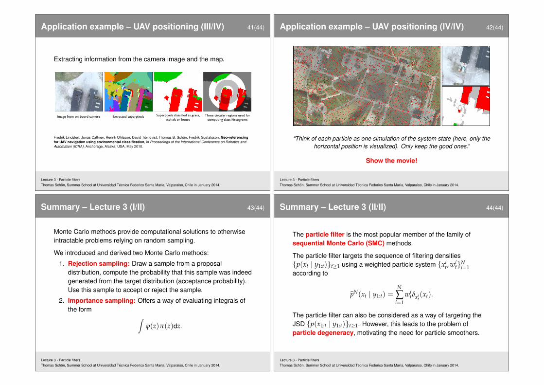
Application example – UAV positioning (III/IV) 41(44)

Extracting information from the camera image and the map.



2. Helicopter pose estimation using a map (II/III)

Image from on-board camera Extracted superpixels Superpixels classified as grass, asphalt or house

Three circular regions used for computing class histograms

Map over the operational environment obtained from

Google Earth.

Manually classified map with grass, asphalt and houses as pre-

specified classes.

Fredrik Lindsten, Jonas Callmer, Henrik Ohlsson, David Törnqvist, Thomas B. Schön, Fredrik Gustafsson, Geo-referencingfor UAV navigation using environmental classification, in Proceedings of the International Conference on Robotics andAutomation (ICRA), Anchorage, Alaska, USA, May 2010.


Application example – UAV positioning (IV/IV) 42(44)



2. Helicopter pose estimation using a map (III/III)

“Think of each particle as one simulation of the system state (in the movie, only the horizontal position is visualized). Only keep the good ones.”

Fredrik Lindsten, Jonas Callmer, Henrik Ohlsson, David Törnqvist, Thomas B. Schön, Fredrik Gustafsson, Geo-referencing for UAV Navigation using Environmental Classification. Proceedings of the International Conference on Robotics and Automation (ICRA), Anchorage, Alaska, USA, May 2010.

“Think of each particle as one simulation of the system state (here, only thehorizontal position is visualized). Only keep the good ones.”

Show the movie!


Summary – Lecture 3 (I/II) 43(44)

Monte Carlo methods provide computational solutions to otherwiseintractable problems relying on random sampling.

We introduced and derived two Monte Carlo methods:

1. Rejection sampling: Draw a sample from a proposaldistribution, compute the probability that this sample was indeedgenerated from the target distribution (acceptance probability).Use this sample to accept or reject the sample.

2. Importance sampling: Offers a way of evaluating integrals ofthe form

∫ϕ(z)π(z)dz.


Summary – Lecture 3 (II/II) 44(44)

The particle filter is the most popular member of the family ofsequential Monte Carlo (SMC) methods.

The particle filter targets the sequence of filtering densities{p(xt | y1:t)}t≥1 using a weighted particle system {xi

t, wit}N

i=1according to

pN(xt | y1:t) =N

∑i=1

witδxi

t(xt).

The particle filter can also be considered as a way of targeting theJSD {p(x1:t | y1:t)}t≥1. However, this leads to the problem ofparticle degeneracy, motivating the need for particle smoothers.


Documents

Outline - Uppsala Universityuser.it.uu.se/~thosc112/CLDS_UTFSM/lecture3handout.… · · 2014-01-20density p ( x t j y: t). lters 2014. Outline 3(44) 1.2 2.xample 3.methods a)sampling