Embed Size (px)
Citation preview

ECE 1767 University of Toronto
l Applicationsl Why Two Fault Simulators Never Agreel General Techniques l Parallel Pattern Simulationl Inactive Fault Removall Critical Path Tracingl Fault Samplingl Statistical Fault Analysis
OutlineOutline
ECE 1767 University of Toronto
ApplicationsApplications
l Fault grading a test setl An aid to an ATPGl Generates knowledge used in some ATPG
systemsl Used to compute coverage loss due to
signature analysisl Generates fault dictionaries for use in fault
diagnosis and location
ECE 1767 University of Toronto
l Since ATPG is much slower than fault simulation, the fault list is trimmed with use of a fault simulator after each vector is generated
AddVectorsto Test Set
SelectNext
Fault
Remove allDetected
Faults
FaultSimulate
Vectors
TestGenerator
TestSet
FaultList
FaultSimulator
Test Generation SystemTest Generation System
ECE 1767 University of Toronto
Fault GradingFault Gradingl It has been shown that the quality of a shipped part
heavily depends on the quality of a test.♦ Defect Level = Reject Rate =♦ c = single stuck-at fault coverage♦ d = defect coverage♦ Assumption: c ≈ d♦ Y = inherent yield of a process = % of chips that are good ♦ defect level = 1 - Y1-c
♦ Current defect levels are 100 to 200 per million.
shipped defective parts total parts shipped as good
defectlevel
1
c50 80 100
decreasingyield

ECE 1767 University of Toronto
Why Two Fault Simulators Why Two Fault Simulators Never AgreeNever Agree
l They simulate different sets of faults.l Some report coverage on the collapsed fault list
rather than the complete (uncollapsed) list.l Fault collapsing algorithms may differ.
♦ Some count ALL gate input and output faults as different, even if a gate output without any fanout is identical to the input of the next gate.
l Coverage reported on different classes of faults (e.g., exclude untestable faults from the fault list).
l Generate less accurate fault lists (e.g., do not distinguish between fanout and stem faults).
ECE 1767 University of Toronto
Why Two Fault Simulators Why Two Fault Simulators Never AgreeNever Agree
l Some include potential detects in the regular fault coverage.
l Some will find a fault definitely detected while others may find it undetected due to inaccuracyin logic simulation involving unknown values
l Some start all flip-flops in a known state, since they do not handle unknowns

ECE 1767 University of Toronto
Fault Coverage MeasuresFault Coverage Measures
NOTE: ‘Untestable’ definition may be tool dependent!
Fault Coverage =Detected Faults
Total Faults
ATG Efficiency =
Testable Coverage = Detected FaultsTotal Faults - Untestable
Detected + Untestable FaultsTotal Faults
ECE 1767 University of Toronto
General TechniquesGeneral Techniques
l Seriall Bit-Parallell Deductivel Concurrentl Parallel concurrentl Parallel Patternl Inactive Fault Removal:
♦ Star Algorithm♦ Critical Path Tracing
ECE 1767 University of Toronto
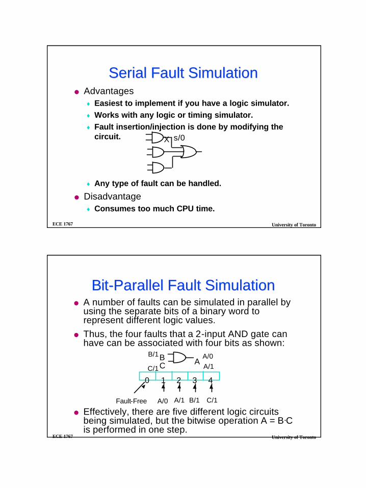
Serial Fault SimulationSerial Fault Simulationl Advantages
♦ Easiest to implement if you have a logic simulator.♦ Works with any logic or timing simulator.♦ Fault insertion/injection is done by modifying the
circuit.
♦ Any type of fault can be handled.
l Disadvantage♦ Consumes too much CPU time.
X s/0
ECE 1767 University of Toronto
BitBit--Parallel Fault SimulationParallel Fault Simulationl A number of faults can be simulated in parallel by
using the separate bits of a binary word to represent different logic values.
l Thus, the four faults that a 2-input AND gate can have can be associated with four bits as shown:
l Effectively, there are five different logic circuits being simulated, but the bitwise operation A = B.C is performed in one step.
BC
B/1
C/1A
A/0A/1
0 1 2 3 4
Fault-Free A/0 A/1 B/1 C/1

ECE 1767 University of Toronto
BitBit--Parallel Fault SimulationParallel Fault Simulationl If the word size W is smaller than the number of
faults NF, then a parallel fault simulator has to do multiple passes.
l 31 faults and the fault-free circuit are typically simulated in parallel using the bitwise parallelism of the computer word:
♦ Actually need two words to encode 3 values: 0, 1, x
g f1 f2 ... f31
g f1 f2 ... f31
g f1 f2 ... f31
v1
v2
v3 ...
32-bit-word
ECE 1767 University of Toronto
BitBit--Parallel Fault SimulationParallel Fault Simulationl Fault injection done using masks.
♦ If fault needs to be injected on line then override the line value by fault value.
Xi/0
0 0 0 0 1 0 0 0 0 0 0
v
m
c
i
xx x x x x x x x x0
v’ = v.m + m.c

ECE 1767 University of Toronto
BitBit--Parallel Fault Simulation Parallel Fault Simulation ExampleExample
l Simulate faults for inputs ABCDEF = 000001
AB
CD
EF
G
H
I
J
K
X XX
G
H
J
I
K
G/1H/1
J/1J/0Fault-Free
ECE 1767 University of Toronto
Deductive Fault SimulationDeductive Fault Simulationl Based on the concept of fault-list propagation.l We associate with each node a list of faults that are
detectable at that node.l When we simulate a gate, we propagate the fault
lists at its inputs to its output.l The output fault list is deduced from those at
inputs.l Key attributes:
♦ one pass, carry all faults at the same time♦ carry only active faults♦ symbolic representation of faults♦ basic operations used: set ∩, U, and difference

ECE 1767 University of Toronto
Deductive Fault SimulationDeductive Fault SimulationLA: {a,c,f}
LB: {d,f,g}
1
1LZ = {a,c,d,f,g}
LZ = LA U LB
LA: {a,c,f}
LB: {d,f,g}
0
1LZ = {a,c}
LZ = LA - LB = LA ∩ LB
{all faults in A which are not in B}
LA: {a,c,f}
LB: {d,f,g}
0
0LZ = { f }
LZ = LA ∩ LB
ECE 1767 University of Toronto
Deductive Fault SimulationDeductive Fault SimulationLA: {a,c,f}
LB: {d,f,g}
0
0LZ = {a,c,d,f,g}
LZ = LA U LB
LA: {a,c,f}
LB: {d,f,g}
1
0LZ = {a,c}
LZ = LA - LB = LA ∩ LB
{all faults in A which are not in B}
LA: {a,c,f}
LB: {d,f,g}
1
1LZ = { f }
LZ = LA ∩ LB
LZ = LILI

ECE 1767 University of Toronto
Deductive Fault Simulation: Deductive Fault Simulation: Fault InjectionFault Injection
LA
LB
A
BLZZ
LA
LB
A
BLZZ
LZ = LA U LB U {Z/0}
LZ = LA - LB U {Z/1}
LZ = {LA ∩ LB} U {Z/1}
LZ = LB - LA U {Z/1}
LZ = LA U LB U {Z/1}
LZ = LA - LB U {Z/0}
LZ = {LA ∩ LB} U {Z/0}
LZ = LB - LA U {Z/0}
A=0, B=0
A=0, B=1
A=1, B=0
A=1, B=1
ECE 1767 University of Toronto
Deductive Fault Simulation ExampleDeductive Fault Simulation Example
j
ba
fch
d
g
k
l
m
n
p
1
111
1
11
1
1
10
e
h0 = {e0,b0,f0,h0 }m0 = {i0,k0,m0 }
n0 = {l0,g0,n0 }
Excited faults:
collapsed fault list withequivalence classes
a0 = {a0 }c0 = {c0 }
p0 = {p0 }
i
j0 = {j0 }

ECE 1767 University of Toronto
Deductive Fault Simulation ExampleDeductive Fault Simulation Example
j
ba
fc
h
d
g
k
l
m
n
p
1
11
1
1
1
1
1
1
10
e h0
m0
p0
n0
a0
c0j0
i
ECE 1767 University of Toronto
Deductive Fault Simulation Deductive Fault Simulation with Unknownswith Unknowns
l Less pessimistic (two lists per node)
{ }0 1
1
LZ = LA U LB1AB Z
{ }U
{ }0 { }U LZ = {LA - LB } U {LB - LA }
0
U
0 0
0 0U U
1
U
LZ = LA U LBUAB Z
LZ = LB - LA - LA
0
1
0 0
01 U
LA
LB
LA
LB
0
0 1
U

ECE 1767 University of Toronto
Deductive Fault Simulation Deductive Fault Simulation with Unknownswith Unknowns
l More pessimistic (single list per node)♦ If good value is unknown, then no fault propagates
on that line.
♦ If faulty value is unknown, mark fault with * and follow propagation rules below.
1
U
UAB Z
LA
LB
LA
LB
0
0 1
U
forces the list to ∅
1->0
1->U
1->0AB Z
ff* f
1->0
1->U
1->UAB Z
f
f* f*
f ∩ f* = f* f U f* = f f - f* = f* f* - f = ∅g ∩ f* = ∅ g U f* = {g,f*} g - f* = g f* - g = f*
use same rulesas for 2-valuedeductive fault simulation
ECE 1767 University of Toronto
Sequential Circuits and FeedbackSequential Circuits and Feedback
l A fault list L containing fault α/0 may propagate back to line α which now has a good value of 0. Then fault α/0 must be removed from the list.
D QXα/0
L 1
1
1/0 0/1 10
1/0 0/1 1/1 0/1
time ttime t+1
remove fault effect

ECE 1767 University of Toronto
PerformancePerformancel In theory, deductive fault simulation can be very
efficient.♦ One pass simulates all faults.♦ Only active faults that will cause events are
present in the list.
l However, lists can be very large.♦ Must implement efficient set union, intersection.♦ Keep lists sorted so that operations are linear.
l Very hard to extend to non-logical fault behavior, e.g., multi-valued levels, hard to incorporate timing (essentially 0-delay simulator).
ECE 1767 University of Toronto
Concurrent Fault SimulationConcurrent Fault Simulationl Like deductive fault simulation, this is also a
one-pass approach, given enough memory, but several passes are often required in practice.
l Only those gates in the faulty circuit whose inputs/outputs are different from the fault-free circuit are (explicitly) simulated.♦ Input and output values are stored for these
gates.♦ The simulation algorithm is similar to event-
driven logic simulation, but events are for the fault-free and faulty circuits.

ECE 1767 University of Toronto
Concurrent Fault SimulationConcurrent Fault Simulation
l Concurrent fault simulation is faster, but more memory intensive than deductive fault simulation.
l Various timing models can be incorporated, so asynchronous circuits can be simulated accurately.
01 1
100
100
11 0
9
12
45
fault listordered byfault index
fault-free gate
ECE 1767 University of Toronto
Parallel Concurrent Fault SimulationParallel Concurrent Fault Simulation
l Faults are evaluated in parallel in groups of size w, where w is the size of the computer word.
l Fault effects are propagated using concurrent fault simulation algorithm.
l Faster and less memory than concurrent fault simulation.

ECE 1767 University of Toronto
Parallel Pattern Fault SimulationParallel Pattern Fault Simulation
l For combinational circuits onlyl Evaluate 32 patterns (test vectors) in parallel
for each fault♦ vectors can be applied in any order
s evaluate good circuits inject fault and evaluate
l Used in random testing♦ keep vector that detects fault
l Used in commercial fault simulator available from Mentor Graphics
ECE 1767 University of Toronto
Inactive Fault RemovalInactive Fault Removal
l Temporarily removing faults known to be inactive in a given time frame will speed up the fault simulation.
l Any faults having different states from the fault-free circuit must be simulated.

ECE 1767 University of Toronto
Inactive Fault RemovalInactive Fault Removall Local Analysis:
X
0
1
11
stuck-at-0
Fault excited but notpropagated two levels
two-level inactiveX0
stuck-at-0
Fault not excited
zero-level inactive
X01
stuck-at-0
Fault excited but notpropagated one level
one-level inactive
ECE 1767 University of Toronto
Inactive Fault RemovalInactive Fault Removal
l Global Analysis: Star Algorithm [Akers, Krishnamurthy, Park, Swaminathan, ITC, 1990]♦ Evaluate good circuit♦ Place Star (*) on subset of nodes which
adequately justify primary output values♦ Nodes not marked * are inactive, and faults on
these nodes cannot be detected

ECE 1767 University of Toronto
Star Algorithm for Star Algorithm for Combinational CircuitsCombinational Circuits
1
1 0
11
11
1
1
0
00
0
0
0*
*
**
***
**
* 1
d
d
d
d
d = don’t care
ECE 1767 University of Toronto
Star AlgorithmStar Algorithml Mark all outputs * (essential to justify the value)
l Back propagate *’s to primary inputs using the following rules:
l All lines not marked * are not required to determine the outputs; hence, no faults on unstarred lines can be detected.
0
0 1
**
1
1 0
*1
0 1
*
0
1 1
*
**
*
*choose one arbitrarily
**
if at least one branch has *, mark stem with *

ECE 1767 University of Toronto
Star Star BacktracingBacktracing for for Sequential CircuitsSequential Circuits
111
1
*
000
0*** *
***
10u
0
*
10u
1
*
*
*
**
**
u1u
u
*
0uu
u**
*
d
ddd
ECE 1767 University of Toronto
Star Algorithm ExampleStar Algorithm Example
0
1
1
1
1

ECE 1767 University of Toronto
Star AlgorithmStar Algorithm
l Theorem: All single and multiple stuck-at faults marked with “d” during a single execution of the algorithm are not detected by the vector and they need not be simulated
l Theorem: All single stuck-at faults marked with “d” in the union of many executions of the algorithm for different runs are also not detected
ECE 1767 University of Toronto
Critical Path TracingCritical Path Tracing[Abramovici, Menon, Miller, IEEE D&T, 1984]
l Identify critical lines in circuit to implicitly determine detected faults for each test vector.
l Perform logic simulation, identify sensitive inputs of each gate, then backtrace from the primary outputs, connecting the dots.
l Exact algorithm for fanout-free circuits, but requires stem analysis for circuits with reconvergent fanout
l It can act as a “sandwich” with Star Algorithm to speed fault simulation

ECE 1767 University of Toronto
Critical Path TracingCritical Path Tracingl Gate input is sensitive if complementing its value it changes the
value of the gate output. A line l has critical value v for test vector t iff t detects the fault l stuck-at-v’
l Lemma: If the output of a gate is critical then all sensitive inputsfor this gate are also critical
ALGORITHM
Simulate a vector and from every primary output, mark it as critical andTrace backwards towards primary inputs marking sensitive lines asCritical according to the lemma
ECE 1767 University of Toronto
Critical Path Tracing: ExampleCritical Path Tracing: Example0
1
0
0
00
00
01
1
1
1 11
1
1
Sensitivelines
ECE 1767 University of Toronto
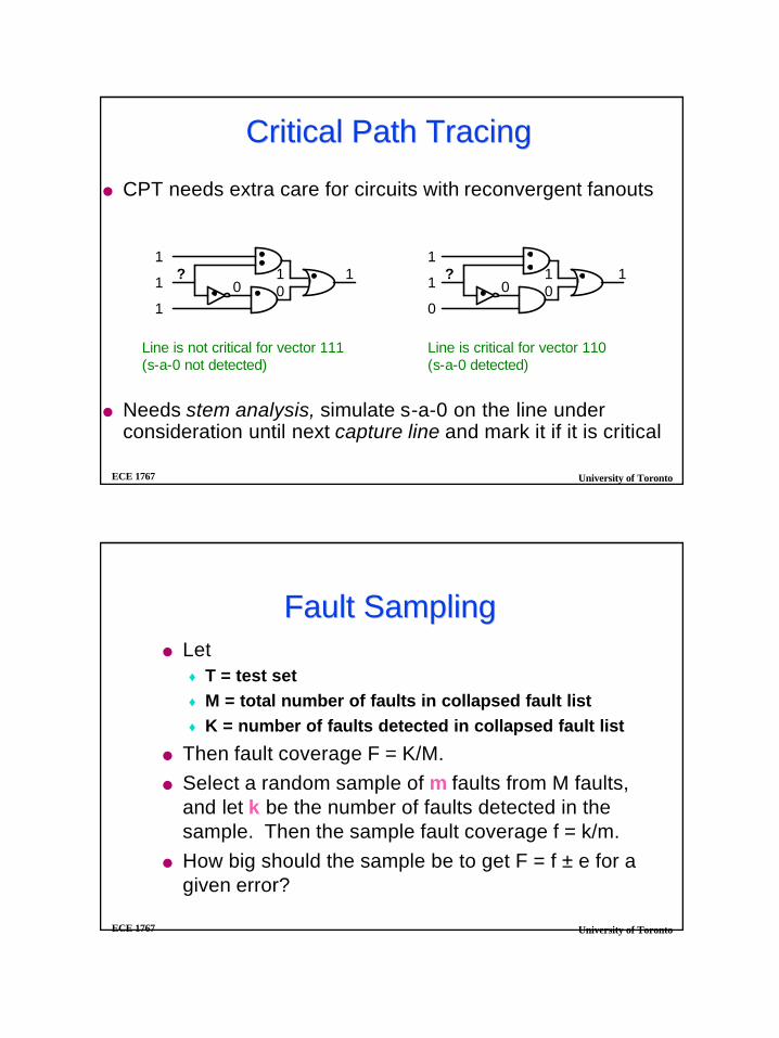
Critical Path TracingCritical Path Tracing
l CPT needs extra care for circuits with reconvergent fanouts
l Needs stem analysis, simulate s-a-0 on the line under consideration until next capture line and mark it if it is critical
? ?
10 01
11 1
1
1 1 1
00 0
Line is not critical for vector 111(s-a-0 not detected)
Line is critical for vector 110(s-a-0 detected)
ECE 1767 University of Toronto
Fault SamplingFault Samplingl Let
♦ T = test set♦ M = total number of faults in collapsed fault list♦ K = number of faults detected in collapsed fault list
l Then fault coverage F = K/M.l Select a random sample of m faults from M faults,
and let k be the number of faults detected in the sample. Then the sample fault coverage f = k/m.
l How big should the sample be to get F = f ± e for a given error?

ECE 1767 University of Toronto
Fault SamplingFault Sampling
l Probability that test T will detect k faults in a random sample of size m is: K
kM - Km - k
Mm
( )( )( )
0.05maxerror
e
0.5 10
m=2000
m=1000
Fault Coverage F
M >> m
ECE 1767 University of Toronto
Statistical Fault Analysis (STAFAN)Statistical Fault Analysis (STAFAN)l No fault simulation is performed
♦ Only a good circuit simulation is performed.♦ Based on signal probabilities.
l Let T = test set of n independent random vectorsl df = probability that a random vector from T detects
the fault fl Probability that none of the n vectors detects f =
(1-df)n
l Then the probability dfn of detecting f by n vectors
= 1 - (1-df)n
not power, just a notation

ECE 1767 University of Toronto
Statistical Fault Analysis (STAFAN)Statistical Fault Analysis (STAFAN)l The the expected number of faults detected (Dn)
from a set Φ of faults is: Dn = ∑(1- (1-df)n)
l Expected fault coverage = Dn
l How to compute df?
f ∈ Φ
| Φ |
ab
c
d
e
f g
hXs/0
Pa = probability of signal a being 1
df = Pc Pd (1-Pf) Ph assuming independent events
ECE 1767 University of Toronto
Statistical Fault Analysis (STAFAN)Statistical Fault Analysis (STAFAN)l 1-Controllability of line l = C1(l) = probability that a
randomly selected vector from T produces logic 1 on line l.
l C0(l) = 1 - C1(l) if no unknowns.l O(l) = observability of line l = probability that a
randomly selected vector from T propagates the fault effect from l to a primary output (PO).
l During good circuit simulation, keep 0-count, 1-count
C0(l) = 0-countn C1(l) = 1-count
n
(signal probabilities)

ECE 1767 University of Toronto
Statistical Fault Analysis (STAFAN)Statistical Fault Analysis (STAFAN)l We also keep a sensitization count on each gate
input♦ S(l) = probability that line l is sensitized to next gate
l Observability of l = S(l) O(m) O(PO) = 1♦ Traverse backwards from PO’s to compute
l11
mline l is sensitized
l l1l2
l3
O(l1)
O(l2)O(l3)
?O(l)
lower bound: O(l) = max O(lk)
upper bound:O(l) = O(l1) + O(l2) - O(l1)(l2)(assuming independent lines)
ECE 1767 University of Toronto
Statistical Fault Analysis (STAFAN)Statistical Fault Analysis (STAFAN)l Detection probabilities for line/fault l/0, l/1
♦ dl/0 = C1(l) O(l)♦ dl/1 = C0(l) O(l)
l Group faults in 3 ranges:♦ high range: df > 0.9 --> considered detected♦ low range: df < 0.1 --> considered not detected♦ middle range: 0.1 < df < 0.9 --> undecided
l Experimental results [Jain and Singer, 1986]♦ 91% to 98% of high range indeed detected♦ 78% to 98% of low range not detected♦ middle range contained 10% of faults on average