CHAPTER9 SORTING(1)

2

Outline

introduction Sorting Networks Bubble Sort and its Variants

3

Introduction

Sorting is the most common operations performed by a computer

Internal or external

Comparison-based Θ(nlogn) and non comparison-based Θ(n)

4

background

Where the input and output sequence are stored?stored on one processdistributed among the process

○ Useful as an intermediate step

What’s the order of output sequence among the processes?Global enumeration

5

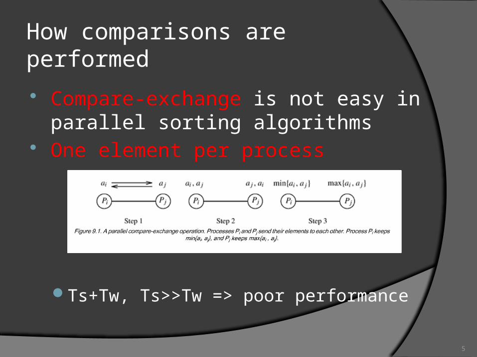
How comparisons are performed Compare-exchange is not easy in parallel

sorting algorithms One element per process

Ts+Tw, Ts>>Tw => poor performance

6

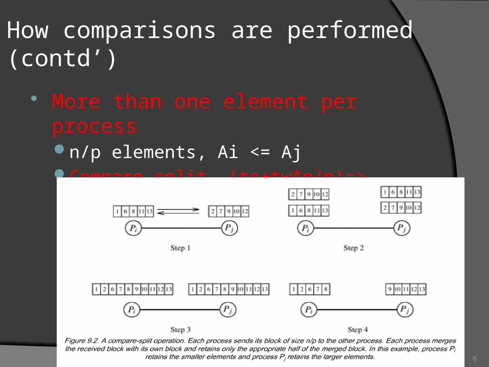
How comparisons are performed (contd’)

More than one element per processn/p elements, Ai <= AjCompare-split, (ts+tw*n/p)=> Ɵ(n/p)

7

Outline

introduction Sorting Networks

Bitonic sortMapping bitonic sort to hypercube and mesh

Bubble Sort and its Variants

8

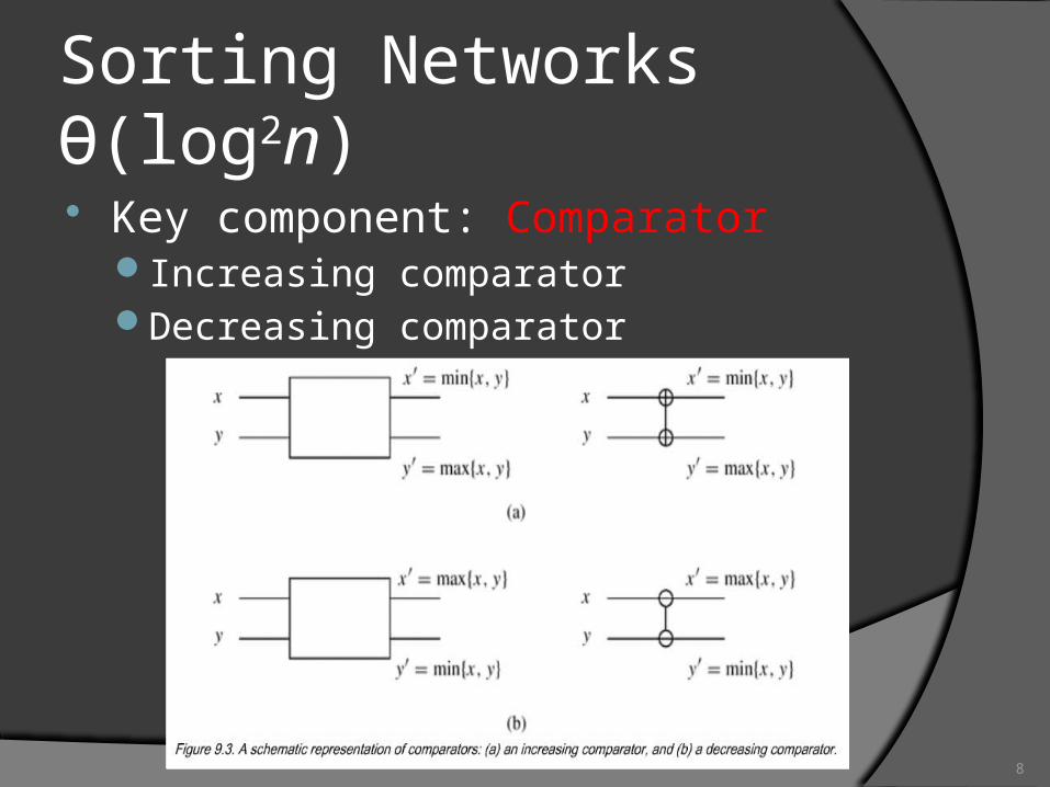
Sorting Networks Ɵ(log2n)

Key component: ComparatorIncreasing comparatorDecreasing comparator

9

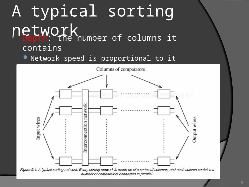
A typical sorting network Depth: the number of columns it contains

Network speed is proportional to it

10

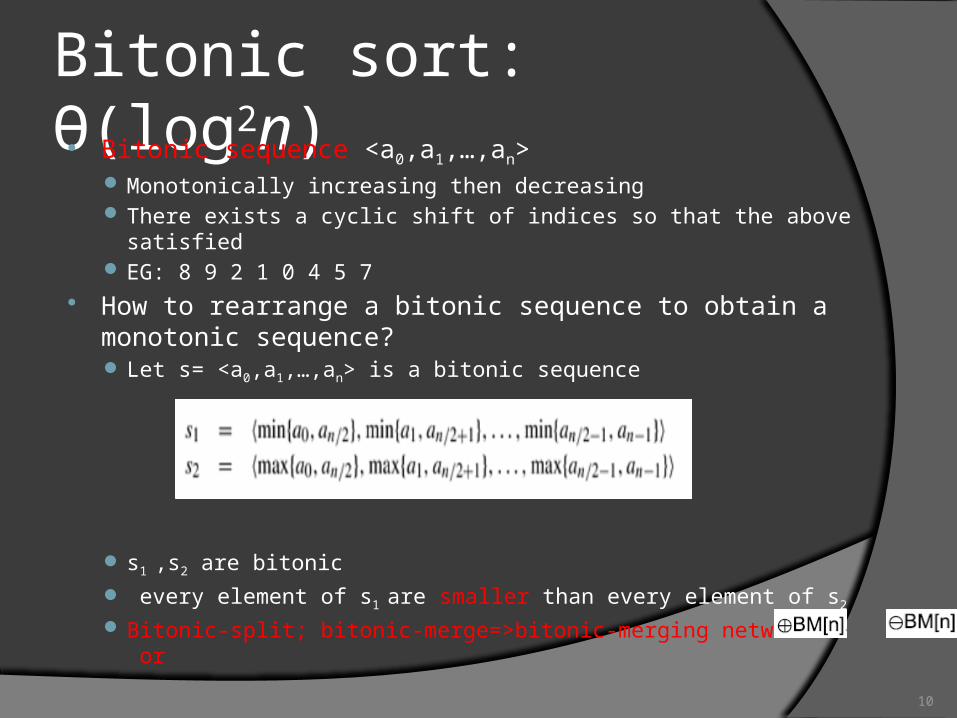
Bitonic sort: Ɵ(log2n) Bitonic sequence <a0,a1,…,an>

Monotonically increasing then decreasing There exists a cyclic shift of indices so that the above satisfied EG: 8 9 2 1 0 4 5 7

How to rearrange a bitonic sequence to obtain a monotonic sequence? Let s= <a0,a1,…,an> is a bitonic sequence

s1 ,s2 are bitonic

every element of s1 are smaller than every element of s2

Bitonic-split; bitonic-merge=>bitonic-merging network or

11

Example of bitonic merging

12

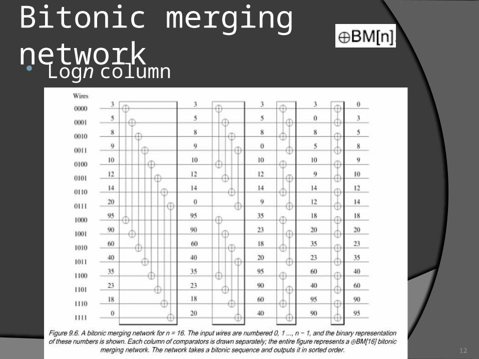
Bitonic merging network Logn column

13

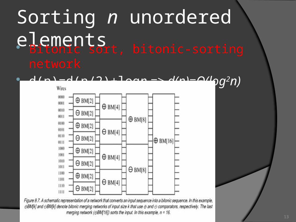
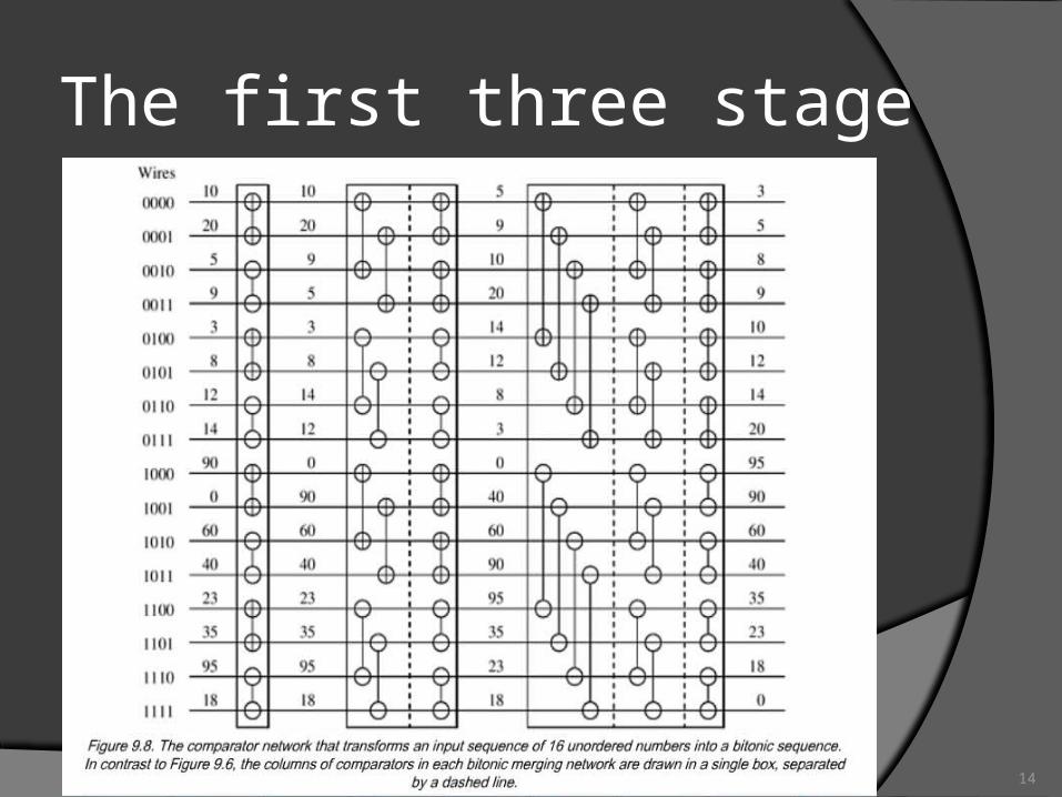
Sorting n unordered elements Bitonic sort, bitonic-sorting network d(n)=d(n/2)+logn => d(n)=Θ(log2n)

14

The first three stage

15

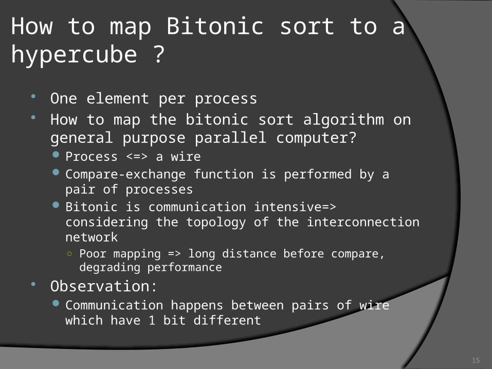
How to map Bitonic sort to a hypercube ?

One element per process How to map the bitonic sort algorithm on general

purpose parallel computer? Process <=> a wire Compare-exchange function is performed by a pair of

processes Bitonic is communication intensive=> considering the

topology of the interconnection network○ Poor mapping => long distance before compare, degrading

performance

Observation: Communication happens between pairs of wire which

have 1 bit different

16

The last stage of bitonic sort

17

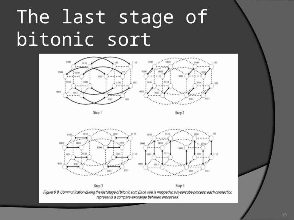
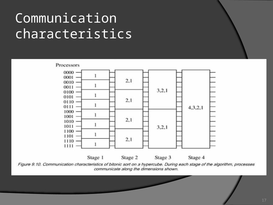
Communication characteristics

18

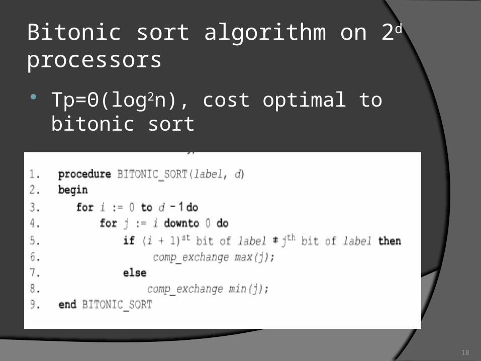
Bitonic sort algorithm on 2d processors Tp=Θ(log2n), cost optimal to bitonic sort

19

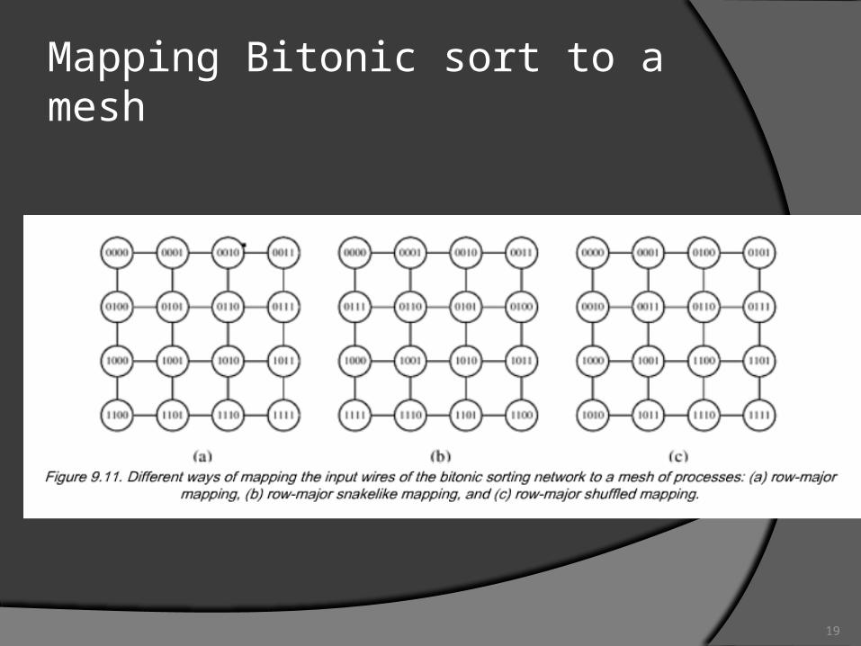
Mapping Bitonic sort to a mesh

20

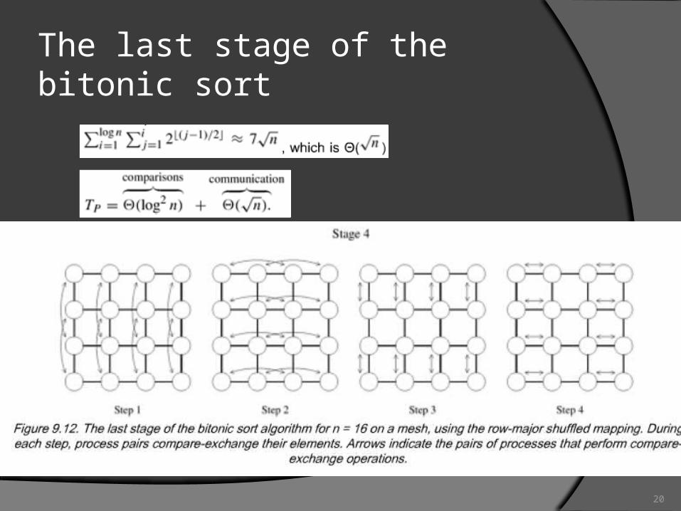
The last stage of the bitonic sort

21

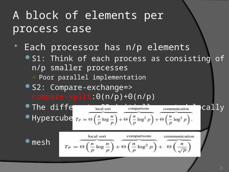
A block of elements per process case Each processor has n/p elements

S1: Think of each process as consisting of n/p smaller processes○ Poor parallel implementation

S2: Compare-exchange=> compare-split:Θ(n/p)+Θ(n/p)The different: S2 initially sorted locallyHypercube

mesh

22

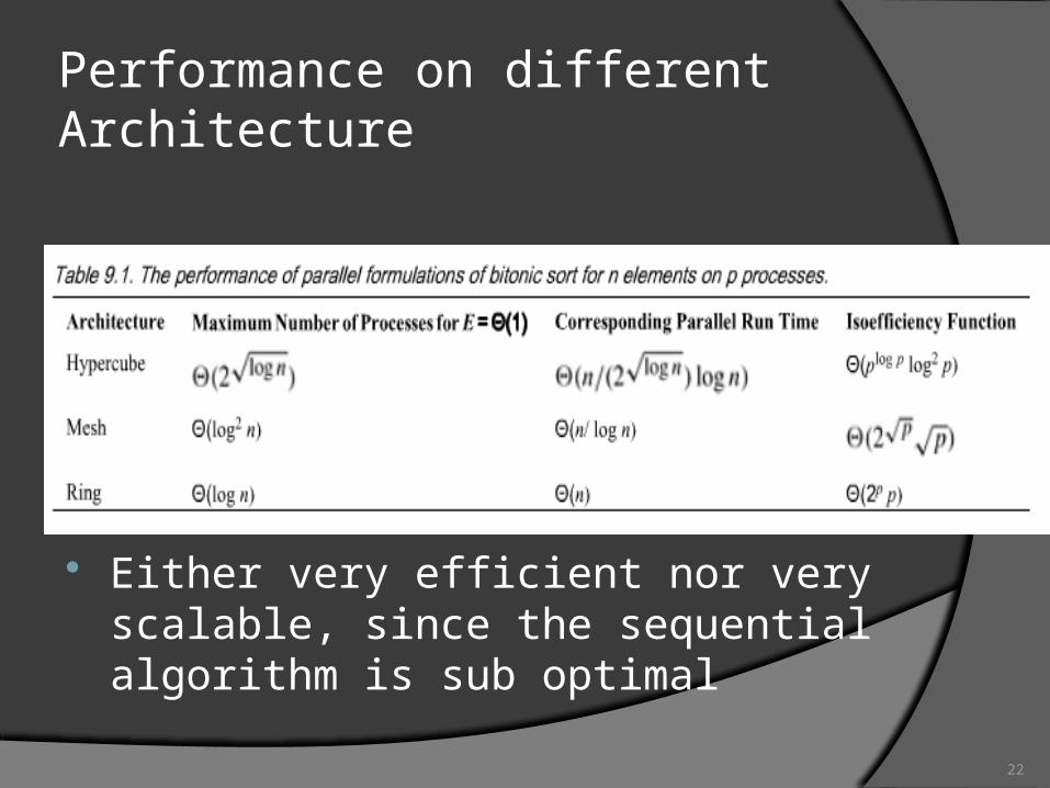
Performance on different Architecture

Either very efficient nor very scalable, since the sequential algorithm is sub optimal

23

Outline

introduction Sorting Networks Bubble Sort and its Variants

24

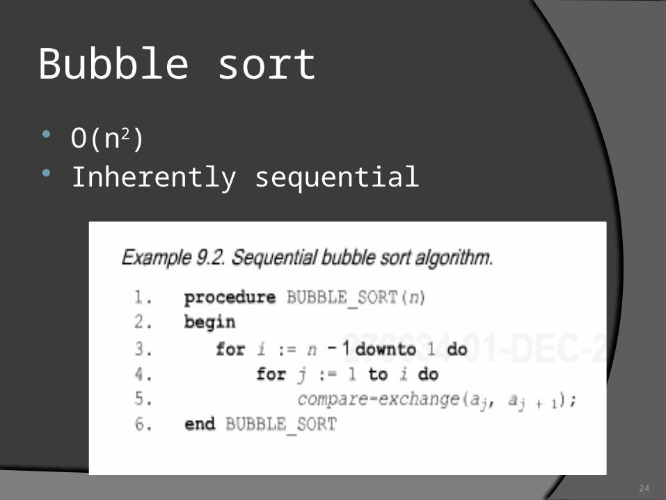
Bubble sort

O(n2) Inherently sequential

25

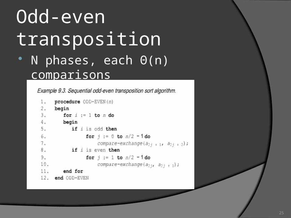
Odd-even transposition

N phases, each Θ(n) comparisons

26

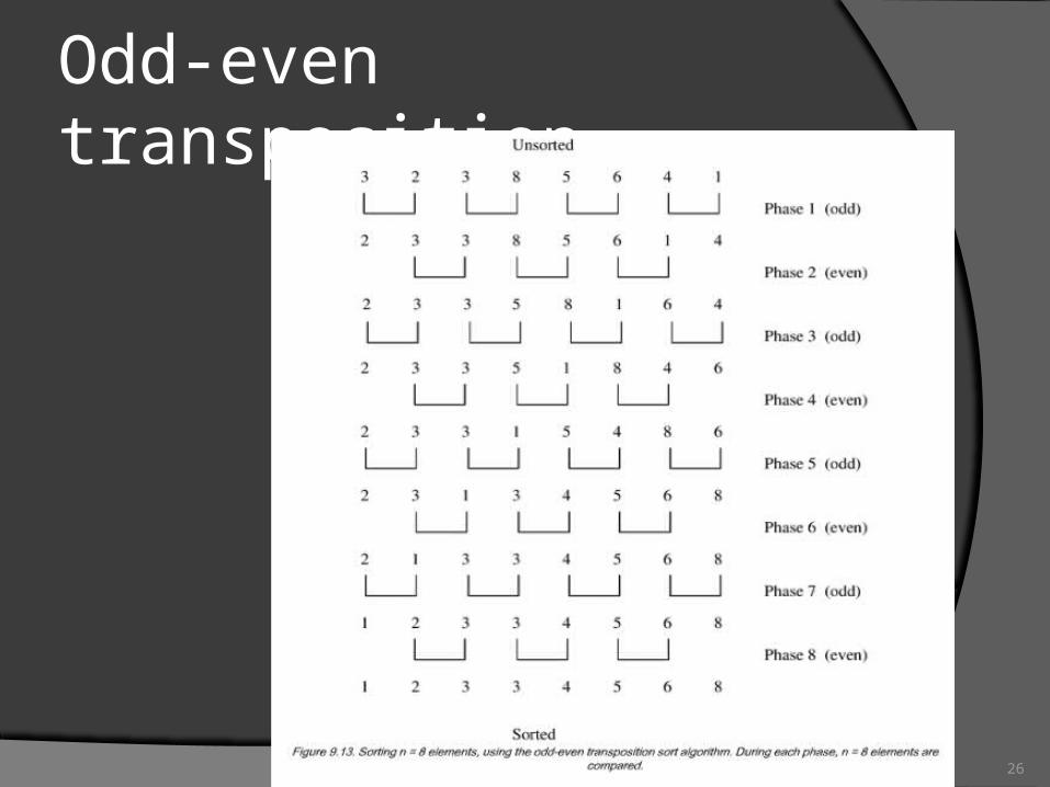
Odd-even transposition

27

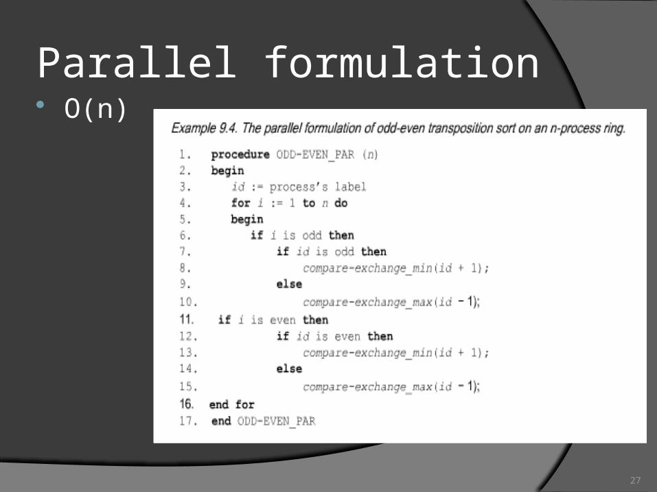
Parallel formulation O(n)

28

Shellsort

Drawback of odd-even sortA sequence which has a few elements out of

order, still need Θ(n2) to sort. idea

Add a preprocessing phase, moving elements across long distance

Thus reduce the odd and even phase

29

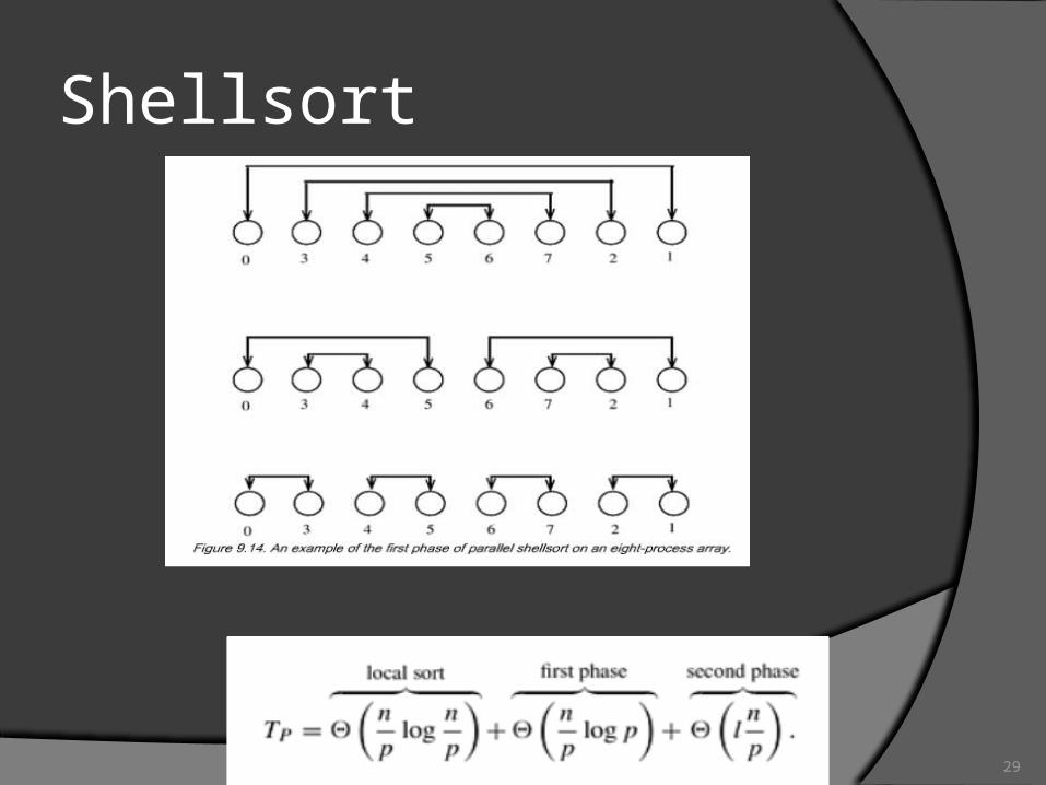
Shellsort

30

Conclusion

Sorting NetworksBitonic networkMapping to hypercube and mesh

Bubble Sort and its VariantsOdd-even sortShell sort

CHAPTER9 SORTING(2)

32

Outline

Issues in Sorting Sorting Networks Bubble Sort and its Variants

Quick sort Bucket and Sample sort Other sorting algorithms

33

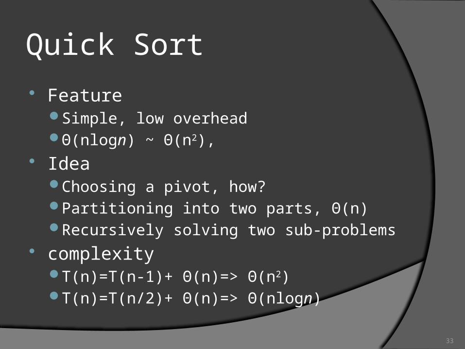
Quick Sort

FeatureSimple, low overheadΘ(nlogn) ~ Θ(n2),

IdeaChoosing a pivot, how? Partitioning into two parts, Θ(n)Recursively solving two sub-problems

complexityT(n)=T(n-1)+ Θ(n)=> Θ(n2)T(n)=T(n/2)+ Θ(n)=> Θ(nlogn)

34

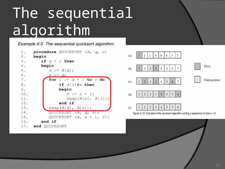
The sequential algorithm

35

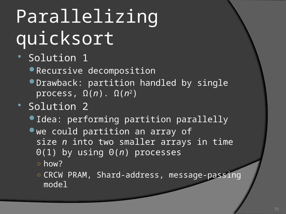
Parallelizing quicksort Solution 1

Recursive decompositionDrawback: partition handled by single process,

Ω(n). Ω(n2) Solution 2

Idea: performing partition parallelly we could partition an array of size n into two smaller

arrays in time Θ(1) by using Θ(n) processes○ how?○ CRCW PRAM, Shard-address, message-passing

model

36

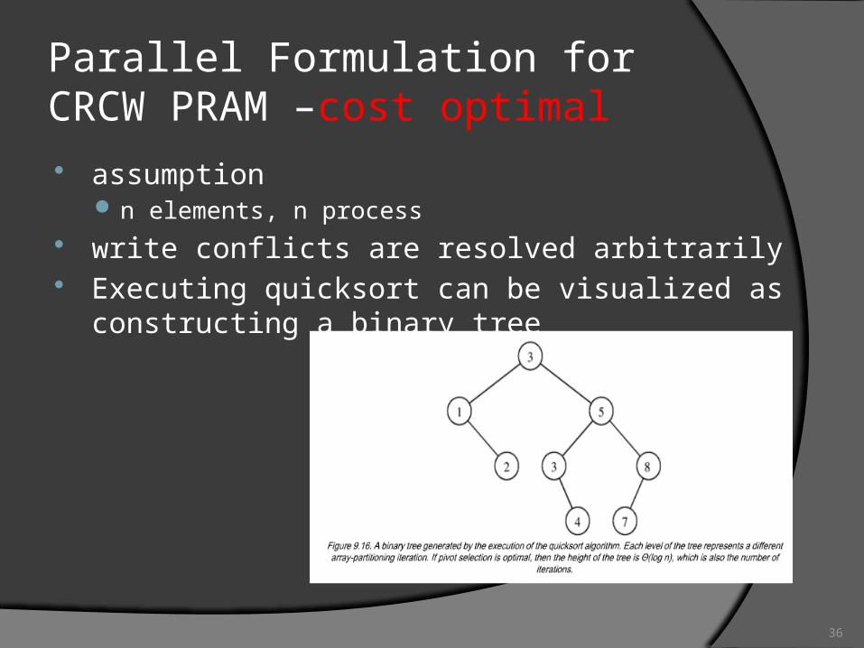
Parallel Formulation for CRCW PRAM –cost optimal assumption

n elements, n process write conflicts are resolved arbitrarily Executing quicksort can be visualized as constructing a

binary tree

37

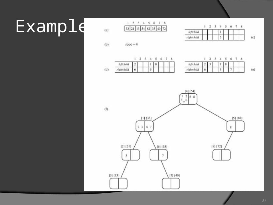
Example

38

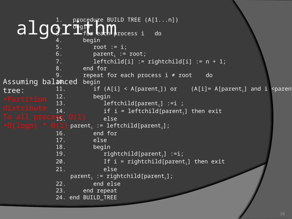
algorithm1. procedure BUILD TREE (A[1...n]) 2. begin 3. for each process i do 4. begin 5. root := i; 6. parenti := root; 7. leftchild[i] := rightchild[i] := n + 1; 8. end for 9. repeat for each process i ≠ root do 10. begin 11. if (A[i] < A[parenti]) or (A[i]= A[parenti] and i <parenti) then 12. begin 13. leftchild[parenti] :=i ; 14. if i = leftchild[parenti] then exit 15. else

parenti := leftchild[parenti]; 16. end for 17. else 18. begin 19. rightchild[parenti] :=i; 20. If i = rightchild[parent i] then exit 21. else

parenti := rightchild[parenti]; 22. end else 23. end repeat 24. end BUILD_TREE

Assuming balanced tree:•Partition distributeTo all process O(1)•Θ(logn) * Θ(1)

39

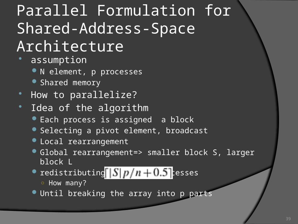
Parallel Formulation for Shared-Address-Space Architecture assumption

N element, p processes Shared memory

How to parallelize? Idea of the algorithm

Each process is assigned a block Selecting a pivot element, broadcast Local rearrangement Global rearrangement=> smaller block S, larger block L redistributing blocks to processes

○ How many?    Until breaking the array into p parts

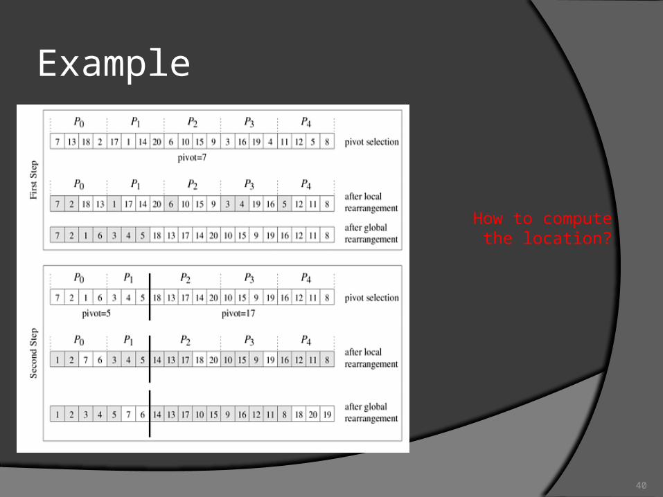
40

Example

How to compute the location?

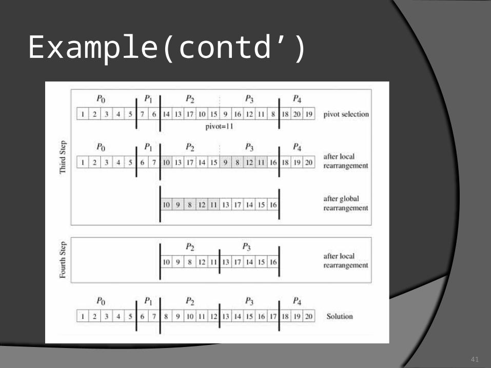
41

Example(contd’)

42

How to do global rearrangement?

43

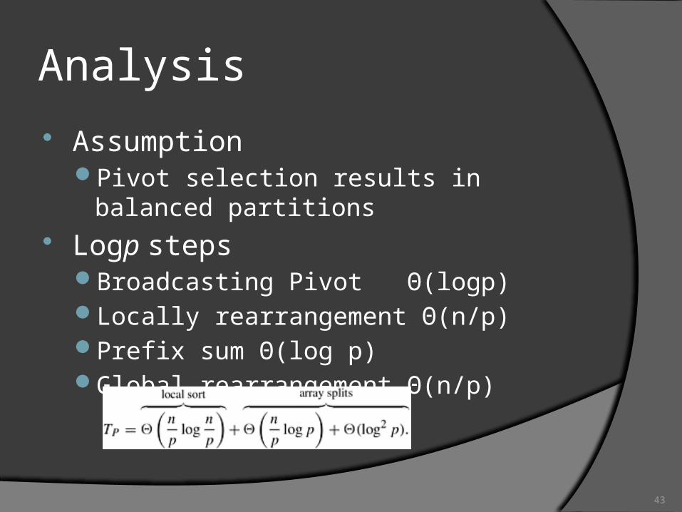
Analysis

AssumptionPivot selection results in balanced partitions

Logp stepsBroadcasting Pivot Θ(logp)Locally rearrangement Θ(n/p) Prefix sum Θ(log p)Global rearrangement Θ(n/p)

44

Parallel Formulation for Message Passing Architecture Similar to shared-address architecture Different

Array distributed to p processes

45

Pivot selection

Random selectionDrawback: bad pivot lead to significant

performance degradation

Median selectionAssumption: the initial distribution of

elements in each process is uniform

46

Outline

Issues in Sorting Sorting Networks Bubble Sort and its Variants

Quick sort Bucket and Sample sort Other sorting algorithms

47

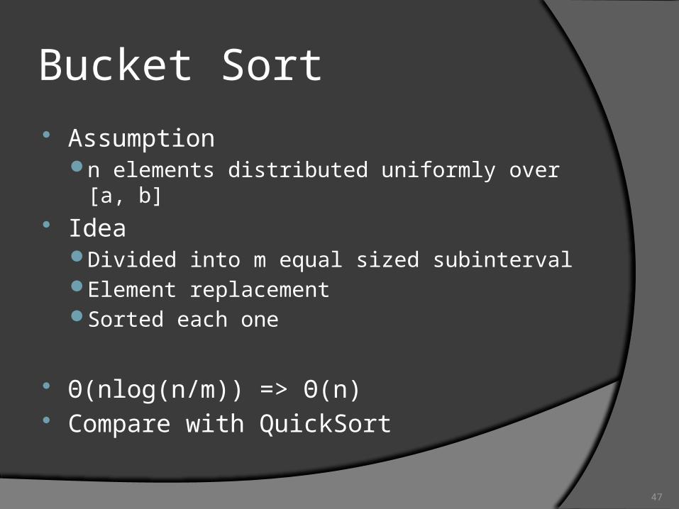
Bucket Sort

Assumptionn elements distributed uniformly over [a, b]

IdeaDivided into m equal sized subintervalElement replacementSorted each one

Θ(nlog(n/m)) => Θ(n) Compare with QuickSort

48

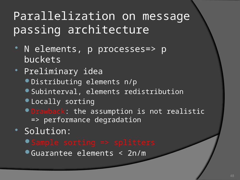
Parallelization on message passing architecture

N elements, p processes=> p buckets Preliminary idea

Distributing elements n/pSubinterval, elements redistributionLocally sortingDrawback: the assumption is not realistic =>

performance degradation

Solution: Sample sorting => splittersGuarantee elements < 2n/m

49

Example

50

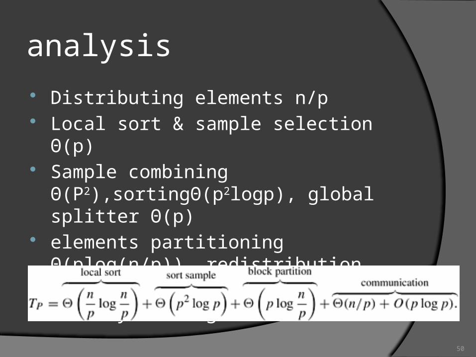
analysis Distributing elements n/p Local sort & sample selection Θ(p) Sample combining Θ(P2),sortingΘ(p2logp),

global splitter Θ(p) elements partitioning Θ(plog(n/p)),

redistribution O(n)+O(plogp) Locally sorting

51

Outline

Issues in Sorting Sorting Networks Bubble Sort and its Variants

Quick sort Bucket and Sample sort Other sorting algorithms

52

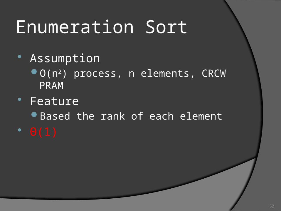
Enumeration Sort

AssumptionO(n2) process, n elements, CRCW PRAM

FeatureBased the rank of each element

Θ(1)

53

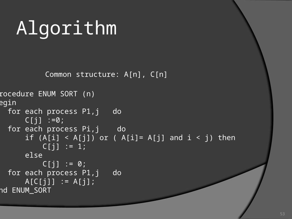
Algorithm

1. procedure ENUM SORT (n) 2. begin 3. for each process P1,j do 4. C[j] :=0; 5. for each process Pi,j do 6. if (A[i] < A[j]) or ( A[i]= A[j] and i < j) then 7. C[j] := 1; 8. else 9. C[j] := 0; 10. for each process P1,j do 11. A[C[j]] := A[j]; 12. end ENUM_SORT

Common structure: A[n], C[n]

54

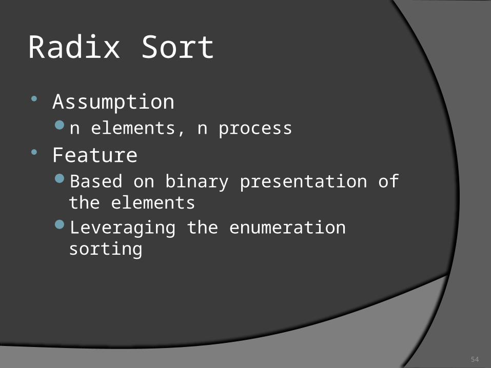
Radix Sort

Assumption n elements, n process

FeatureBased on binary presentation of the

elementsLeveraging the enumeration sorting

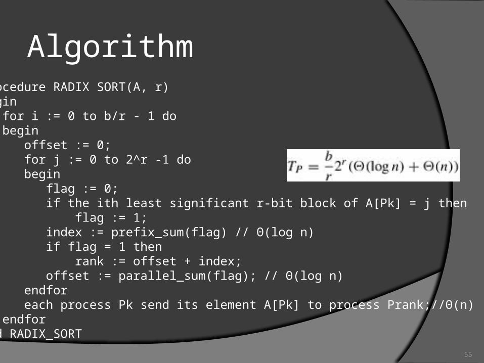
55

Algorithm1. procedure RADIX SORT(A, r) 2. begin 3. for i := 0 to b/r - 1 do 4. begin 5. offset := 0; 6. for j := 0 to 2^r -1 do 7. begin 8. flag := 0; 9. if the ith least significant r-bit block of A[Pk] = j then 10. flag := 1; 11. index := prefix_sum(flag) // Θ(log n) 12. if flag = 1 then 13. rank := offset + index; 14. offset := parallel_sum(flag); // Θ(log n)15. endfor 16. each process Pk send its element A[Pk] to process Prank;//Θ(n) 17. endfor 18. end RADIX_SORT

56

Conclusion Sorting Networks

Bitonic network, mapping to hypercube and mesh Bubble Sort and its Variants

Odd-even sorting, shell sorting Quick sort

Parallel formation on CRCW PRAM, shared address/MP architecutre

Bucket and Sample sort Enumeration and radix sorting