J Math Chem (2010) 47:891–909DOI 10.1007/s10910-009-9609-2

ORIGINAL PAPER

Outliers detection in the statistical accuracy testof a pKa prediction

Milan Meloun · Sylva Bordovská · Karel Kupka

Received: 24 November 2008 / Accepted: 8 September 2009 / Published online: 19 September 2009© Springer Science+Business Media, LLC 2009

Abstract The regression diagnostics algorithm REGDIA in S-Plus is introducedto examine the accuracy of pKa predicted with four programs: PALLAS, MARVIN,PERRIN and SYBYL. On basis of a statistical analysis of residuals, outlier diagnosticsare proposed. Residual analysis of the ADSTAT program is based on examining good-ness-of-fit via graphical diagnostics of 15 exploratory data analysis plots, such as barplots, box-and-whisker plots, dot plots, midsum plots, symmetry plots, kurtosis plots,differential quantile plots, quantile-box plots, frequency polygons, histograms, quan-tile plots, quantile-quantile plots, rankit plots, scatter plots, and autocorrelation plots.Outliers in pKa relate to molecules which are poorly characterized by the consideredpKa program. Of the seven most efficient diagnostic plots (the Williams graph, Graphof predicted residuals, Pregibon graph, Gray L–R graph, Index graph of Atkinsonmeasure, Index graph of diagonal elements of the hat matrix and Rankit Q–Q graph ofjackknife residuals) the Williams graph was selected to give the most reliable detectionof outliers. The six statistical characteristics, Fexp, R2, R2

P, MEP, AIC, and s in pKaunits, successfully examine the specimen of 25 acids and bases of a Perrin’s data setclassifying four pKa prediction algorithms. The highest values Fexp, R2, R2

P and thelowest value of MEP and s and the most negative AIC have been found for PERRINalgorithm of pKa prediction so this algorithm achieves the best predictive power andthe most accurate results. The proposed accuracy test of the REGDIA program canalso be extended to test other predicted values, as log P , log D, aqueous solubility orsome physicochemical properties.

M. Meloun (B) · S. BordovskáDepartment of Analytical Chemistry, Faculty of Chemical Technology, Pardubice University,532 10 Pardubice, Czech Republice-mail: milan.meloun@upce.cz

K. KupkaTriloByte Statistical Software, s.r.o., Jiráskova 21, 530 02 Pardubice, Czech Republic

123

892 J Math Chem (2010) 47:891–909

Keywords pKa prediction · Dissociation constants · Outliers · Residuals ·Goodness-of-fit · Williams graph

1 Introduction

The principle of the structure–property relationship is a basic concept in organic chem-istry, as the properties of molecules are intrinsically determined by their structure. Themacroscopic properties of chemical compounds clearly depend on their microscopicstructural descriptors, and the development of a Quantitative Structure/Property Rela-tionship QSPR on theoretical descriptors is a powerful tool for the prediction of thechemical, physical and biological properties of compounds. An enormous number ofstructural descriptors have been used by researchers to increase the ability to correlatevarious properties. A molecule is transformed into a sequence or a fixed-length vectorof values before it can be used to conduct QSPR studies. Although molecular size mayvary to a large extent, the vector representation must be in a fixed length for all themolecules in a data set in order to apply a data analysis method. Various approacheshave been developed to represent the structure of molecules for QSPR studies. Since somany descriptors are available, the development and selection of appropriate descrip-tors in describing a selected property of molecule has become a Herculean task. Animportant role of the degree of ionization in the biological behaviour of chemical sub-stances, namely drugs, is well established. One of the fundamental properties of anorganic drug molecule, the pKa value, determines the degree of dissociation in solution[1–12]. To obtain a significant correlation and accurately predicted pKa, it is crucialthat appropriate structural descriptors be employed. In this context, the approach usinga statistical accuracy examination of the predicted pKa is important.

Numerous studies have considered, and various approaches have been used inthe prediction of pKa, but mostly without a rigorous statistical test of pKa accuracy[13–35].

The goal of this paper is to develop a rigorous accuracy examination tool which isable to investigate weather a pKa prediction method leads to a sufficiently accurateestimate of pKa value, as the correlation between predicted pKa,pred and experimentalvalue pKa,exp is usually very high. In this examination, the linear regression models areused for interpreting the essential features of a set of pKa,pred data. There are a numberof common difficulties associated with real datasets. The first involves the detectionand elucidation of outlying pKa,pred values in the predicted pKa data. A problemwith pKa,pred outliers is that they can strongly influence the regression model, espe-cially when using least squares criteria, so several steps are required: firstly to identifywhether there are any pKa,pred values that are atypical of the dataset, then to removethem, and finally to interpret their deviation from the straight line regression model.

Because every prediction is based on a congeneric parent structure, pKa valuescan only be reliably predicted for compounds very similar to those in the training set,making it difficult or impossible to get good estimates for novel structures. A furtherdisadvantage is the need to derive a very large number of fragment constants and cor-relation factors, a process which is complicated and potentially ambiguous. Although

123

J Math Chem (2010) 47:891–909 893

this is probably the most widely used method, the accuracy and extensibility of thepredictions obtained have not been gratifying.

Authors usually evaluate model quality and outliers on the basis of fitted residues.A simple criticism criterion like, for example, “more than 80% of pKa in the trainingsample are predicted with an accuracy of within one log unit of their measurement,and 95% are within two log units of the accuracy,” is often used, or “when the dif-ference between the measured pKa,exp and predicted pKa,pred values is larger than 3log units, it is used to denote a discrepancy”. However, rigorous statistical detection,assessment, and understanding of the outliers in pKa,pred values are major problemsof interests in an accuracy examination. The goal of any pKa,pred outlier detection isto find this true partition and, thus, separate good from outlying pKa values. A singlecase approach to the detection of outliers can, however, fail because of masking orswamping effects, in which outliers go undetected because of the presence of other,usually adjacent, pK ′

as. Masking occurs when the data contain outliers which we failto detect; this can happen because some of the outliers are hidden by other outliers inthe data. Swamping occurs when we wrongly declare some of the non-outlying pointsto be outliers [36]; this occurs because outliers tend to pull the regression equationtoward them, thereby making other points further from the fitted equation. Maskingis therefore a false negative decision, whereas swamping is a false positive. Unfortu-nately, a bewilderingly large number of statistical tests, diagnostic graphs and residualplots have been proposed for diagnosting influential points, namely outliers, and it istime to select those approaches that are appropriate for pKa prediction. This paperprovides a critical survey of many outlier diagnostics, illustrated with data examplesto show how they successfully characterize the joint influence of a group of cases andto yield a better understanding of joint influence.

2 Methods

2.1 Software and data used

Several software packages for pKa prediction were used and tested in this study. Mostof the work was carried out on PALLAS [10], MARVIN [15], Perrin method [29] andSYBYL [14] software packages, based mostly on chemical structure, the reliabilityof which reflects the accuracy of the underlying experimental data. In most softwarethe input is the chemical structure drawn in a graphical mode. For the accuracy exam-ination of pKa,pred values we used Perrin’s examples of different chemical classes asan external data set [29]. The model predicted pKa values were compared to Perrin’spredictions, and the experimental measurements are listed in Table 1.

For the creation of regression diagnostic graphs and computation of the regressionbased characteristics, the REGDIA algorithm was written in S-Plus [37], and the Lin-ear Regression module of our ADSTAT package [38] was used. We have tried to showsome effective drawbacks of the statistical diagnostic tools in REGDIA which are,in our experience, able to correctly pinpoint influential points. One should concen-trate on that diagnostic tool which measures the impact on the quantity of primaryinterest. The main difference between the use of regression diagnostics and classical

123

894 J Math Chem (2010) 47:891–909

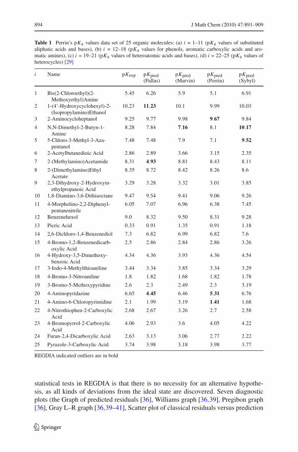
Table 1 Perrin’s pKa values data set of 25 organic molecules: (a) i = 1–11 (pKa values of substitutedaliphatic acids and bases), (b) i = 12–18 (pKa values for phenols, aromatic carboxylic acids and aro-matic amines), (c) i = 19–21 (pKa values of heteroatomic acids and bases), (d) i = 22–25 (pKa values ofheterocycles) [29]

i Name pKexp pKpred(Pallas)

pKpred(Marvin)

pKpred(Perrin)

pKpred(Sybyl)

1 Bis(2-Chloroethyl)(2-Methoxyethyl)Amine

5.45 6.26 5.9 5.1 6.91

2 1-(4’-Hydroxycyclohexyl)-2-(Isopropylamino)Ethanol

10.23 11.23 10.1 9.99 10.03

3 2-Aminocycloheptanol 9.25 9.77 9.98 9.67 9.84

4 N,N-Dimethyl-2-Butyn-1-Amine

8.28 7.84 7.16 8.1 10.17

5 5-Chloro-3-Methyl-3-Aza-pentanol

7.48 7.48 7.9 7.1 9.52

6 2-Acetylbutanedioic Acid 2.86 2.89 3.66 3.15 2.35

7 2-(Methylamino)Acetamide 8.31 4.93 8.81 8.43 8.11

8 2-(Dimethylamino)EthylAcetate

8.35 8.72 8.42 8.26 8.6

9 2,3-Dihydroxy-2-Hydroxym-ethylpropanoic Acid

3.29 3.28 3.32 3.01 3.85

10 1,8-Diamino-3,6-Dithiaoctane 9.47 9.54 9.41 9.06 9.26

11 4-Morpholino-2,2-Diphenyl-pentanenitrile

6.05 7.07 6.96 6.38 7.45

12 Benzenehexol 9.0 8.32 9.50 8.31 9.28

13 Picric Acid 0.33 0.91 1.35 0.91 1.18

14 2,6-Dichloro-1,4-Benzenediol 7.3 6.82 6.99 6.82 7.6

15 4-Bromo-1,2-Benzenedicarb-oxylic Acid

2.5 2.86 2.84 2.86 3.26

16 4-Hydroxy-3,5-Dimethoxy-benzoic Acid

4.34 4.36 3.93 4.36 4.54

17 3-Iodo-4-Methylthioaniline 3.44 3.34 3.85 3.34 3.29

18 4-Bromo-3-Nitroaniline 1.8 1.82 1.68 1.82 1.78

19 3-Bromo-5-Methoxypyridine 2.6 2.3 2.49 2.3 3.19

20 4-Aminopyridazine 6.65 4.45 6.46 5.31 6.76

21 4-Amino-6-Chloropyrimidine 2.1 1.99 3.19 1.41 1.68

22 4-Nitrothiophen-2-CarboxylicAcid

2.68 2.67 3.26 2.7 2.58

23 4-Bromopyrrol-2-CarboxylicAcid

4.06 2.93 3.6 4.05 4.22

24 Furan-2,4-Dicarboxylic Acid 2.63 3.13 3.06 2.77 2.22

25 Pyrazole-3-Carboxylic Acid 3.74 3.98 3.18 3.98 3.77

REGDIA indicated outliers are in bold

statistical tests in REGDIA is that there is no necessity for an alternative hypothe-sis, as all kinds of deviations from the ideal state are discovered. Seven diagnosticplots (the Graph of predicted residuals [36], Williams graph [36,39], Pregibon graph[36], Gray L–R graph [36,39–41], Scatter plot of classical residuals versus prediction

123

J Math Chem (2010) 47:891–909 895

[36,39–41], Index graph of jackknife residuals [36], and Index graph of Atkinson dis-tance [41]) were selected as the most efficient to give reliable influential point detectionresults and four being powerful enough to separate influential points into outliers andhigh-leverages.

2.2 Regression diagnostics for examining the pKa accuracy in REGDIA

The examination of pKa data quality involves detection of the influential points in theregression model proposed pKa,pred = β0 + β1pKa,exp, which cause many problemsin regression analysis by shifting the parameter estimates or increasing the varianceof the parameters [36]: (i) pKa,pred-outliers, which differ from the other points in theirvalue on the y-axis, where y stands in all of the following relations for pKa,pred; (ii)high-leverage points, which differ from the other points in their value on the x-axis,where x stands in all of the following relations for pKa,exp, or (iii) both outliers andhigh-leverages, standing for a combination of both together. Analysis of various typesof residuals in the REGDIA program is useful for detecting inadequacies in the model,or influential points in the data [36]:

(a) Ordinary residuals ei are defined by ei = yi − xiβ, where xi is the i th row ofmatrix pK a,exp.

(b) Normalized residuals eN ,i = ei/s(e) are often recommended for outlier detec-tion.

(c) Standardized residuals eS,i = ei/(s(e)√

1 − hi i exhibit constant unit variance,and their statistical properties are the same as those of ordinary residuals.

(d) Jackknife residuals eJ,i = eS,i

√n−m−1

n−m−e2S,i

are residuals, where n stands for the

number of points and m for the number of parameters, here m − 2 and for whicha rule is valid: strongly influential points have squared jackknife residuals e2

J,igreater than 10. The descriptive statistics of residuals can be used for a numericalgoodness-of-fit evaluation in REGDIA program, cf. page 290 in Vol. 2 of [36]:

(1) The residual bias is the arithmetic mean of residuals E(e) and should be equalto zero.

(2) The square-root of the residuals variance s2(e) = RSS(b)/(n − m) is used toestimate of the residual standard deviation, s(e), where RSS(b) is the residualsquare-sum, should be of the same magnitude as the random error s(pKa,pred) asit is valid that s(e) ≈ s(pKa,pred).

(3) The determination coefficient D calculated from the correlation coefficient R andmultiplied by 100% is interpreted as the percentage of points which correspondto proposed regression model.

(4) One of the most efficient criterion is the mean quadratic error of prediction

MEP =

n∑i=1

(yi − xTi b(i))

2

n, (1)

123

896 J Math Chem (2010) 47:891–909

where b(i) is the estimate of regression parameters when all points except thei th were used and xi (here pKa,exp,i) is the i th row of matrix pK a,exp. The sta-tistic MEP uses a prediction y P,i (here pKa,pred,i) from an estimate constructedwithout including the i th point.

(5) The MEP (Eq. 1) can be used to express the predicted determination coefficient,

R2P = 1 − n × MEP

n∑i=1

y2i − n × y2

. (2)

(6) Another statistical characteristic is derived from information theory and entropy,and is known as the Akaike information criterion,

AIC = n ln

(RSS(b)

n

)+ 2m, (3)

where n is the number of data points and m is the number of parameters, for astraight line, m = 2. The best regression model is considered to be that in whichthe minimal value of MEP and AIC and the highest value of the R2

P are reached.

Individual estimates b of parameters β are then tested for statistical significanceusing the Student t-test. The Fisher-Snedecor F-test of significance of the regressionmodel proposed is based on the testing criterion

FR = R2(n − m)/[(1 − R2)(m − 1)

](4)

which has a Fisher-Snedecor distribution with (m − 1) and (n − m) degrees of free-dom, where R2 is the determination coefficient. With the use of FR the null hypothesisH0 : R2 = 0 may be tested and concerns a test of significance of all regression param-eters β.

Examination of data and model quality can be considered directly from the scatterplot of pKa,pred vs. pKa,exp. For the analysis of residuals a variety of plots have beenwidely used in regression diagnostics of REGDIA program:

(a) the overall index plot of classical residuals gives an initial impression of theresiduals trend in chronological order. If the straight line model is correct, theresiduals e form a random pattern and should resemble values from a normaldistribution with zero mean. To examine the normality of a residual distribution,the quantile-quantile (rankit) plot may be applied;

(b) the graph of predicted residuals indicates outliers as points located on the linex = y, i.e. here pKa,pred = pKa,exp but far from its central pattern;

(c) the Williams graph has two boundary lines, the first for outliers, y = t0.95(n −m−1) and the second for high-leverages, x = 2m/n. Note that t0.95(n−m−1) isthe 95% quantile of the Student distribution with (n−m −1) degrees of freedom;

(d) the Pregibon graph classifies two levels of influential points: strongly influen-tial points are above the upper line, while medium influential points are locatedbetween the two lines;

123

J Math Chem (2010) 47:891–909 897

(e) Gray’s L–R graph indicates outliers as points situated close above the corner ofthe triangle;

(f) the scatter plot of classical residuals indicates only suspicious points which couldbe proven as outliers using other diagnostics;

(g) the index graph of jackknife residuals indicates outliers according to an empiriccriterion which states: “strongly influential outliers reach a jackknife residualgreater than 3”;

(h) the scatter plot of the Atkinson distance d leads to numerically similar values asthe jackknife residuals, and therefore its interpretation is similar.

2.3 Graphs for the exploratory analysis of residuals in ADSTAT [36,38]

Residual analysis is based on examining goodness-of-fit via graphical and/or numeri-cal diagnostics in order to check the data and model quality. A variety of exploratorydata analysis plots, such as bar plots, box-and-whisker plots, dot plots, midsum plots,symmetry plots, kurtosis plots, differential quantile plots, quantile-box plots, frequencypolygon, histogram, quantile plots, quantile-quantile plots, rankit plots, scatter plots,and autocorrelation plots, have been introduced in the ADSTAT program [36,38], andwidely used by authors such as Belsey, Kuh and Welsch [39], Cook and Weisberg[40], Atkinson [41], Chatterjee and Hadi [42], Barnett and Lewis [43], Welsch [44],Weisberg [45], Rousseeuw and Leroy [46]; others may be found Vol. 2 page 289 of[36]. The following plots are quite important as they give an initial impression of thepKa,pred residuals by using computer graphics [36,38]:

(a) The autocorrelation scatter plot, being an overall index plot of residuals checkswhether there is evidence of any trend in a pKa,pred series. The ideal plot showsa horizontal band of points with constant vertical scatter from left to right andindicates the suspicious points that could be influential.

(b) The quantile-box plot for symmetrical distributions has a sigmoid shape, whilefor asymmetrical is convex or concave increasing. A symmetric unimodal distri-bution contains individual boxes arranged symmetrically inside one another, andthe value of relative skewness is close to zero. Outliers are indicated by a suddenincrease of the quantile function outside the quartile F box.

(c) The dot diagram and jittered-dot diagram represent a univariate projection of aquantile plot, and give a clear view of the local concentration of points.

(d) The notched box-and-whisker plot permits determination of an interval estimateof the median, illustrates the spread and skewness of the sample data, shows thesymmetry and length of the tails of distribution and aids the identification ofoutliers.

(e) The symmetry plot gives information about the symmetry of the distribution. Fora fully symmetrical distribution, it forms a horizontal line y = M (median).

(f) The quantile-quantile (rankit)plot has on the x-axis the quantile of the standard-ized normal distribution u Pi for Pi = i/(n + 1), and on the y-axis, has theordered residuals e(i). Data points lying along a straight line indicate distribu-tions of similar shape. This plot enables classification of a sample distributionaccording to its skewness, kurtosis and tail length. A convex or concave shape

123

898 J Math Chem (2010) 47:891–909

indicates a skewed sample distribution. A sigmoidal shape indicates that the taillengths of the sample distribution differ from those of a normal one.

(g) The kernel estimation of probability density plot and the histogram detect anactual sample distribution.

3 Experimental

3.1 Procedure of accuracy examination

The procedure for the examination of influential points in the data, and the construc-tion of a linear regression model with the use of REGDIA and ADSTAT programs,consists of the following steps:

Step 1 Graphs for the exploratory indication of outliers. This step carries out thegoodness-of-fit test by a statistical examination of classical residuals in ADSTAT[36,38] for the identification of suspicious points (S) or outliers (O): the overall indexplot of residuals trend, the quantile plot, the dot diagram and jittered-dot diagram, thenotched box-and-whisker plot, the symmetry plot, the quantile-quantile rankit plot,the histogram and the Kernel estimation of the probability density function also provea symmetry of sample distribution. Sample data lead to descriptive statistics, as theyare the residual mean and the standard deviation of residuals. The Student t-test tests anull hypothesis of zero mean of the residuals bias, H0 : E(e) = 0 vs. HA : E(e) �= 0.

Step 2 Preliminary indication of suspicious influential points. This step discoverssuspicious points only. The index graph of classical residuals and the rankit plot alsoindicate outliers. Beside descriptive statistics E(e) and s the Student t-test for a nullhypothesis a null hypothesis H0 : E(e) = 0 vs. HA : E(e) �= 0 and α = 0.05 is alsoexamined.

Step 3 Regression diagnostics to detect suspicious points or outliers in REGDIAprogram: The least squares straight-line fitting of the regression model proposedpKa,pred = β0 + β1pKa,exp, with a 95% confidence interval, and regression diag-nostics for the identification of outlying pKa,pred values detect suspicious points (S)or outliers (O) using the graph of predicted residuals indicates, the Williams graph,the Pregibon graph, the L–R graph indicates, the scatter plot of classical residuals vsprediction, the index graph of jackknife residuals and the index plot of the Atkinsondistance.

Step 4 Interpretation of outliers. The statistical significance of both parameters β0and β1 of the straight-line regression model pKa,pred = β0(s0, A or R) + β1(s1, Aor R) pKa,exp is tested in REGDIA program using the Student t-test, where A or Rmeans that the tested null hypothesis H0 : β0 = 0 vs. HA : β0 �= 0 and H0 : β1 = 1vs. HA : β1 �= 1 was either Accepted or Rejected. The standard deviations s0 and s1of the actual parameters β0 and β1 are estimated. A statistical test of total regressionis performed using a Fisher-Snedecor F-test and the calculated significance level Pis enumerated. Outliers are indicated with the preferred Williams graph. The corre-lation coefficient R, the determination coefficient R2 giving the regression rabat D

123

J Math Chem (2010) 47:891–909 899

are computed. The mean quadratic error of prediction MEP, the Akaike informationcriterion AIC and the predictive coefficient of determination R2

P as a percentage arecalculated to examine the quality of the model. According to the test for the fulfilmentof the conditions for the least-squares method, and the results of regression diagnos-tics, a more accurate regression model without outliers is constructed and statisticalcharacteristics examined. Outliers should be elucidated.

3.2 Supporting information available

The complete computational procedures of the REGDIA program, input data spec-imens and corresponding output in numerical and graphical form are available freeof charge via the internet at http://meloun.upce.cz in the blocks DATA and ALGO-RITHMS.

4 Results and discussion

The results of the pKa prediction with the use of the four algorithms PALLAS [10],MARVIN [15], PERRIN [29] and SYBYL [13,14] are compared, with the predictedvalues of the dissociation constants pKa,pred are plotted against the experimental val-ues pKa,exp for the compounds of Perrin’s data set from Table 1. Even given thatPALLAS’s performance might be somewhat less accurate for druglike compounds,there is overall a good agreement between the predicted pKa,pred and experimentalvalues pKa,exp.

4.1 Evaluating diagnostics in outlier detection

Regression analysis and the discovery of influential points in the pKa,pred values ofdata have been investigated extensively using the REGDIA program. Perrin’s liter-ature data in Table 1 represent a useful medium for the comparison of results anddemonstrating the efficiency of diagnostic tools for outliers detection. The majorityof multiple outliers are better indicated by diagnostic plots than by statistical tests ofthe diagnostic values in the table. These data have been much analyzed as a test foroutlier methods. The PALLAS-predicted pKa,pred vs experimentally observed pKa,expvalues for the examined set for bases and acids are plotted in Fig. 1a. The pKa,predvalues are distributed evenly around the diagonal, implying consistent error behaviourin the residual values. The optimal slope β1 and intercept β0 of the linear regressionmodel pKa,pred = β0 + β1pKa,exp for β0 = 0.17(0.41) and β1 = 0.94(0.07) canbe understood as 0 and 1, respectively, where the standard deviation of parametersappears in brackets.

Another way to evaluate a quality of the regression model proposed with the useof the PALLAS program is to examine its goodness-of-fit. Most of the acids and basein the examined sample are predicted with an accuracy of better than one log of theirmeasurement. Detecting influential points, two figures, each of 8 diagnostics, wereanalyzed: (i) diagnostic plots based on exploratory data analysis (Fig. 2a–h), and (ii)

123

900 J Math Chem (2010) 47:891–909

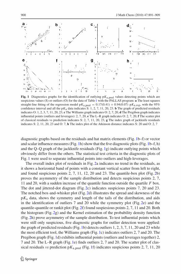
Fig. 1 Diagnostics graphs for the identification of outlying pKa,pred values detecting points which aresuspicious values (S) or outliers (O) for the data of Table 1 with the PALLAS program: a The least squaresstraight-line fitting of the regression model pKa,pred = 0.17(0.41) + 0.94(0.07) pKa,exp, with the 95%confidence interval and all the pKa data indicates S: 1, 2, 7, 11, 20, 23. b The graph of predicted residualsindicates O: 1, 2, 3, 7, 11, 20, 23, c The Williams graph indicates O: 2, 7, 20, d The Pregibon graph indicatesinfluential points (outliers and leverages): 2, 7, 20, e The L–R graph indicates O: 2, 7, 20, f The scatter plotof classical residuals vs prediction indicates S: 2, 7, 11, 20, 23, g The index graph of jackknife residualsindicates S: 2, 11, 20, 23 and O: 7, h The index plot of the Atkinson distance indicates S: 20 and O: 2, 7

diagnostic graphs based on the residuals and hat matrix elements (Fig. 1b–f) or vectorand scalar influence measures (Fig. 1h) show that the five diagnostic plots (Fig. 1b–f, h)and the Q–Q graph of the jackknife residuals (Fig. 1g) indicate outlying points whichobviously differ from the others. The statistical test criteria in the diagnostic plots ofFig. 1 were used to separate influential points into outliers and high-leverages.

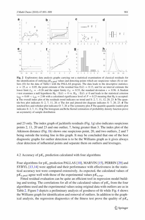
The overall index plot of residuals in Fig. 2a indicates no trend in the residuals, asit shows a horizontal band of points with a constant vertical scatter from left to right,and found suspicious points 2, 7, 11, 12, 20 and 23. The quantile-box plot (Fig. 2b)proves the asymmetry of the sample distribution and detects suspicious points 2, 7,11 and 20, with a sudden increase of the quantile function outside the quartile F box.The dot and jittered-dot diagram (Fig. 2c) indicates suspicious points 7, 20 and 23.The notched box-and-whisker plot (Fig. 2d) illustrates the spread and skewness of thepKa data, shows the symmetry and length of the tails of the distribution, and aidsin the identification of outliers 7 and 20 while the symmetry plot (Fig. 2e) and thequantile-quantile or rankit plot (Fig. 2f) found suspiesious points 2, 7, 11 and 20. Boththe histogram (Fig. 2g) and the Kernel estimation of the probability density function(Fig. 2h) prove asymmetry of the sample distribution. To test influential points whichwere still only suspicious, five diagnostic graphs for outlier detection were applied:the graph of predicted residuals (Fig. 1b) detects outliers 1, 2, 3, 7, 11, 20 and 23 whilethe most efficient tool, the Williams graph (Fig. 1c) indicates outliers 2, 7 and 20. ThePregibon graph (Fig. 1d) exhibits influential points (outliers and leverages together) 2,7 and 20. The L–R graph (Fig. 1e) finds outliers 2, 7 and 20. The scatter plot of clas-sical residuals vs prediction pKa,pred (Fig. 1f) indicates suspicious points 2, 7, 11, 20

123

J Math Chem (2010) 47:891–909 901

Fig. 2 Exploratory data analysis graphs carrying out a statistical examination of classical residuals forthe identification of outlying pKa,pred values and detecting points which are suspicious values (S) or out-liers (O) for the data of Table 1 with the PALLAS program. The data leads to the descriptive statistics:n = 25, α = 0.05, the point estimate of the residual bias E(e) = 0.13, and for an interval estimate thelower limit L L = −0.26 and the upper limity LU = 0.53, the standard deviation s = 0.96. A Studentt-test examines a null hypothesis H0 : E(e) = 0 vs. HA : E(e) �= 0 and leads to the statistical criteriontexp = 0.69 < tcrit = 2.06 with a calculated significance level of P = 0.23 meaning that H0 is accepted:a The overall index plot of the residuals trend indicates no trend and S: 2, 7, 11, 12, 20, 23. b The quan-tile-box plot indicates S: 2, 7, 11, 20. c The dot and jittered-dot diagram indicates S: 7, 20, 23. d Thenotched box-and-whisker plot indicates O: 7, 20. e The symmetry plot, f The quantile-quantile (rankit) plotindicates S: 2, 7, 11, 20 g The histogram and h the Kernel estimation of probability density function provean asymmetry of sample distribution

and 23 only. The index graph of jackknife residuals (Fig. 1g) also indicates suspiciouspoints 2, 11, 20 and 23 and one outlier, 7, being greater than 3. The index plot of theAtkinson distance (Fig. 1h) shows one suspicious point, 20, and two outliers, 2 and 7being outside the testing line in this graph. It may be concluded that one of the bestdiagnostic graphs for outlier detection is to be the Williams graph as it gives alwaysclear detection of influential points and separate them on outliers and leverages.

4.2 Accuracy of pKa prediction calculated with four algorithms

Four algorithms for pKa prediction PALLAS [10], MARVIN [15], PERRIN [29] andSYBYL [13,14] were applied and their performance with effectiveness in the statis-tical accuracy test were compared extensively. As expected, the calculated values ofpKa,pred agree well with those of the experimental values pKa,exp.

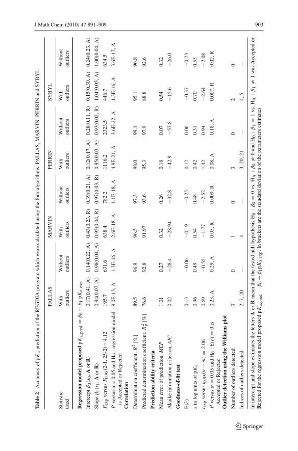
Fitted residual evaluation can be quite an efficient tool in regression model build-ing and testing. The correlations for all of the calculated values of pKa from the fouralgorithms used and the experimental values using original data with outliers are as inTable 2. Figure 3 depicts a preliminary analysis of goodness-of-fit while Fig. 4 showsthe Williams graph for identification and removal of outliers. In addition to the graph-ical analysis, the regression diagnostics of the fitness test prove the quality of pKa

123

902 J Math Chem (2010) 47:891–909

Fig. 3 Comparison of four programs for the detection of outlying pKa,pred values using the index graphof classical residuals (a, b, c, d in the upper part of figure) and the rankit Q–Q plot (e, f, g, h) for the dataof Table 1. A Student t-test tests a null hypothesis H0 : E(e) = 0 vs. HA : E(e) �= 0 and for n = 25and α = 0.05 the descriptive statistics are calculated: a PALLAS: E(e) = 0.13, s = 0.96, test leading totexp = 0.69 < tcrit = 2.06, P = 0.23(H0 is accepted), suspicious pKa,pred values indicated 1, 2, 7, 11, 20,23. b MARVIN: E(e) = −0.19, s = 0.54, test leading to texp = | − 1.77| < tcrit = 2.06, P = 0.05 (H0is accepted), suspicious pKa,pred values indicated: 4, 11. c Perrin: E(e) = 0.12, s = 0.42, test leading totexp = 1.42 < tcrit = 2.06, P = 0.08 (H0 is accepted), suspicious pKa,pred values indicated: 3, 11, 13, 20,21. d SYBYL: E(e) = −0.37, s = 0.70, test leading to texp = | − 2.64| > tcrit = 2.06, P = 0.007 (H0is rejected), suspicious pKa,pred values indicated: 1, 2, 4, 5, 6, 10, 11

prediction. The highest values R2, R2P, the lowest value of MEP and s and the more

negative value of AIC in Fig. 5 and Table 2 are exhibited with the Perrin’s algorithm ofpKa prediction, and this algorithm has the best predictive power and most accurate.

Regression model: The predicted versus the experimentally observed pKa values forexamined data set are plotted in Fig. 4a,b,c,d. The data points are distributed evenlyaround the diagonal in the figures, implying the consistent error behavior of the residualvalue. The slope and intercept of the linear regression are optimal; the slope estimatesfor the four algorithms used areβ1(s1) = 0.94(0.07, A), 0.95(0.04, R), 0.95(0.03, A),

1.04(0.05, A) where A or R means that the tested null hypothesis H0 : β0 = 0 vs. HA :β0 �= 0 and H0 : β1 = 1 vs. HA : β1 �= 1 was Accepted or Rejected with the standarddeviation of parameters estimates in brackets. Removing the outliers from the data setthese estimates reach values 0.98(0.04, A), 0.97(0.03, R), 0.93(0.02, R), 1.00(0.04, A).The intercept estimates are β0(s0) = 0.17(0.41, A), 0.43(0.23, R), 0.12(0.17, A),

0.15(0.30, A) and after removing outliers from data set 0.14(0.22, A), 0.39(0.21,A), 0.28(0.11, R), 0.24(0.23, A). Here A or R means the tested null hypothesisH0 : β0 = 0 vs. HA : β0 �= 0 and H0 : β1 = 1 vs. HA : β1 �= 1 was Acceptedor Rejected. The slope is equal to one for 3 algorithms, excepting MARVIN, andthe intercept is equal to zero for 3 algorithms, again excepting MARVIN. The Fisher-Snedecor F-test of overall regression in Fig. 5 leads to a calculated significance level ofP = 9.0E-13, 2.6E-18, 4.9E-21, 1.3E-16, and after removing the outliers from the data

123

J Math Chem (2010) 47:891–909 903

Tabl

e2

Acc

urac

yof

pK

apr

edic

tion

ofth

eR

EG

DIA

prog

ram

whi

chw

ere

calc

ulat

edus

ing

the

four

algo

rith

ms:

PAL

LA

S,M

AR

VIN

,PE

RR

INan

dSY

BY

L

PAL

LA

SM

AR

VIN

PER

RIN

SYB

YL

Stat

istic

With

With

out

With

With

out

With

With

out

With

With

out

used

outli

ers

outli

ers

outli

ers

outli

ers

outli

ers

outli

ers

outli

ers

outli

ers

Reg

ress

ion

mod

elpr

opos

edp

Ka,

pred

=β

0+

β1

pK

a,ex

p

Inte

rcep

tβ0(s

0,A

orR

)0.

17(0

.41,

A)

0.14

(0.2

2,A

)0.

43(0

.23,

R)

0.39

(0.2

1,A

)0.

12(0

.17,

A)

0.28

(0.1

1,R

)0.

15(0

.30,

A)

0.24

(0.2

3,A

)

Slop

eβ

1(s

1,A

orR

)0.

94(0

.07,

A)

0.98

(0.0

4,A

)0.

95(0

.04,

R)

0.97

(0.0

3,R

)0.

95(0

.03,

A)

0.93

(0.0

2,R

)1.

04(0

.05,

A)

1.00

(0.0

4,A

)

Fex

pve

rsus

F0.

95(2

-1,2

5-2)

=4.

1219

5.7

631.

663

8.4

782.

211

16.2

2323

.544

6.7

634.

5

Pve

rsus

α=

0.05

and

H0

:regr

essi

onm

odel

isA

ccep

ted

orR

ejec

ted

9.0E

-13,

A1.

3E-1

6,A

2.6E

-18,

A1.

1E-1

8,A

4.9E

-21,

A3.

6E-2

2,A

1.3E

-16,

A3.

6E-1

7,A

Cor

rela

tion

Det

erm

inat

ion

coef

ficie

nt,

R2

[%]

89.5

96.9

96.5

97.3

98.0

99.1

95.1

96.8

Pred

icte

dde

term

inat

ion

coef

ficie

nt,

R2 P

[%]

76.6

92.8

91.9

793

.695

.397

.988

.892

.6

Pre

dict

ion

abili

tycr

iter

ia

Mea

ner

ror

ofpr

edic

tion,

ME

P1.

010.

270.

320.

260.

180.

070.

540.

32

Aka

ike

info

rmat

ion

crite

rion

,AIC

0.02

−28.

4−2

8.94

−32.

8−4

2.9

−57.

8−1

5.6

−26.

0

Goo

dnes

s-of

-fit

test

E(e

)0.

13−0

.06

−0.1

9−0

.25

0.12

0.06

−0.3

7−0

.23

sin

log

units

ofp

Ka

0.96

0.49

0.54

0.48

0.42

0.31

0.70

0.53

t exp

vers

ust 0

.95(n

−m

)=

2.06

0.69

−0.5

5−1

.77

−2.5

21.

420.

94−2

.64

−2.0

8

Pve

rsus

α=

0.05

and

H0

:E(e

)=

0is

Acc

epte

dor

Rej

ecte

d0.

23,A

0.29

,A0.

05,R

0.00

9,R

0.08

,A0.

18,A

0.00

7,R

0.02

,R

Out

lier

dete

ctio

nus

ing

the

Will

iam

spl

ot

Num

ber

ofou

tlier

sde

tect

ed3

01

03

02

0

Indi

ces

ofou

tlier

sde

tect

ed2,

7,20

—4

—3,

20,2

1—

4,5

—

Inin

terc

ept

and

slop

ees

timat

esth

ele

tters

Aor

Rm

ean

that

the

test

ednu

llhy

poth

esis

H0

:β0

=0

vs.H

A:β

0�=

0an

dH

0:β

1=

1vs

.HA

:β1

�=1

was

Acc

epte

dor

Rej

ecte

dfo

rth

ere

gres

sion

mod

elpr

opos

edp

Ka,

pred

=β

0+

β1p

Ka,

exp.I

nbr

acke

tsar

eth

est

anda

rdde

viat

ion

ofth

epa

ram

eter

ses

timat

es

123

904 J Math Chem (2010) 47:891–909

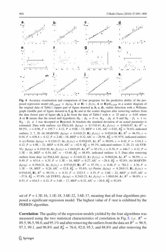
Fig. 4 Accuracy examination and comparison of four programs for the predictive ability of the pro-posed regression model pKa,pred = β0(s0, A or R) + β1(s1, A or R)pKa,exp in a scatter diagram ofthe original data of Table 1 (upper part of figure denoted a, b, c, d), outlier detection with a Williamsgraph (middle part of figure denoted e, f, g, h) and in the scatter diagram after removing outliers fromthe data (lower part of figure ch, i, j, k) from the data of Table 1 with n = 25 and α = 0.05 whereA or R means that the tested null hypothesis H0 : β0 = 0 vs. HA : β0 �= 0 and H0 : β1 = 1 vs.HA : β1 �= 1 was Accepted or Rejected. In brackets the standard deviation of an actual parameter isestimated. Data with outliers: (a) PALLAS: β0(s0) = 0.17(0.41, A), β1(s1) = 0.94(0.07, A), R2 =89.5%, s = 0.96, F = 195.7 > 4.12, P = 9.0E − 13, MEP = 1.01, AIC = 0.02, R2

P = 76.6%, indicated

outliers: 2, 7, 20. (b) MARVIN: β0(s0) = 0.43(0.23, R), β1(s1) = 0.95(0.04, R), R2 = 96.5%, s =0.54, F = 638.4 > 4.12, P = 2.6E−18, MEP = 0.32, AIC = −28.94, R2

P = 91.97%, indicated outliers:

4. (c) Perrin: β0(s0) = 0.12(0.17, A), β1(s1) = 0.95(0.03, A), R2 = 98.0%, s = 0.42, F = 1116.2 >

4.12, P = 4.9E − 21, MEP = 0.18, AIC = −42.9, R2P = 95.3%, indicated outliers: 3, 20, 21. (d) SYB-

YL: β0(s0) = 0.15(0.30, A), β1(s1) = 1.04(0.05, A), R2 = 95.1%, s = 0.70, F = 446.7 > 4.12, P =1.3E − 16, MEP = 0.54, AIC = −15.60, R2

P = 88.8%, indicated outliers: 4, 5. Data after removing

outliers from data: (a) PALLAS: β0(s0) = 0.14(0.22, A), β1(s1) = 0.98(0.04, A), R2 = 96.9%, s =0.49, F = 631.6 > 4.35, P = 1.3E − 16, MEP = 0.27, AIC = −28.4, R2

P = 92.8%, (b) MARVIN:

β0(s0) = 0.39(0.21, A), β1(s1) = 0.97(0.03, R), R2 = 97.3%, s = 0.48, F = 782.2 > 4.30, P =1.1E − 18, MEP = 0.26, AIC =-32.8, R2

P = 93.6%, (c) Perrin: β0(s0) = 0.28(0.11, R), β1(s1) =0.93(0.02, R), R2 = 99.1%, s = 0.31, F = 2323.5 > 4.35, P = 3.6E − 22, MEP = 0.07, AIC =−57.8, R2

P = 97.9%, (d) SYBYL: β0(s0) = 0.24(0.23, A), β1(s1) = 1.00(0.04, A), R2 = 96.8%, s =0.53, F = 634.5 > 4.32, P = 3.6E − 17, MEP = 0.32, AIC = −26.0, R2

P = 92.6%

set of P = 1.3E-16, 1.1E-18, 3.6E-22, 3.6E-17, meaning that all four algorithms pro-posed a significant regression model. The highest value of F-test is exhibited by thePERRIN algorithm.

Correlation: The quality of the regression models yielded by the four algorithms wasmeasured using the two statistical characteristics of correlation in Fig. 5, i.e. R2 =89.5, 96.5, 98.0, and 95.1% and after removing the outliers from the data set R2 = 96.9,97.3, 99.1, and 96.8% and R2

P = 76.6, 92.0, 95.3, and 88.8% and after removing the

123

J Math Chem (2010) 47:891–909 905

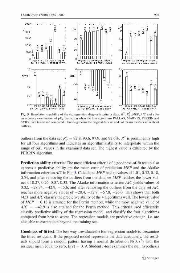
Fig. 5 Resolution capability of the six regression diagnostic criteria Fexp, R2, R2P, MEP, AIC and s for

an accuracy examination of pKa prediction when the four algorithms PALLAS, MARVIN, PERRIN andSYBYL are tested and compared. Here orig means the original data set and out means the data set withoutoutliers

outliers from the data set R2P = 92.8, 93.6, 97.9, and 92.6%. R2 is prominently high

for all four algorithms and indicates an algorithm’s ability to interpolate within therange of pKa values in the examined data set. The highest value is exhibited by thePERRIN algorithm.

Prediction ability criteria: The most efficient criteria of a goodness-of-fit test to alsoexpress a predictive ability are the mean error of prediction MEP and the Akaikeinformation criterion AIC in Fig. 5. Calculated MEP lead to values of 1.01, 0.32, 0.18,0.54, and after removing the outliers from the data set MEP reaches the lower val-ues of 0.27, 0.26, 0.07, 0.32. The Akaike information criterion AIC yields values of0.02, −28.94, −42.9, −15.6, and after removing the outliers from the data set AICreaches more negative values of −28.4, −32.8, −57.8, −26.0. This shows that bothMEP and AIC classify the predictive ability of the 4 algorithms well. The lowest valueof MEP = 0.18 is attained for the Perrin method, while the most negative value ofAIC = −42.9 is also attained for the Perrin method. This criteria used efficientlyclassify predictive ability of the regression model, and classify the four algorithmscompared from best to worst. The regression models are predictive enough, i.e. arealso able to extrapolate beyond the training set.

Goodness-of-fit test: The best way to evaluate the four regression models is to examinethe fitted residuals. If the proposed model represents the data adequately, the resid-uals should form a random pattern having a normal distribution N(0, s2) with theresidual mean equal to zero, E(e) = 0. A Student t-test examines the null hypothesis

123

906 J Math Chem (2010) 47:891–909

H0 : E(e) = 0 vs. HA : E(e) �= 0 and gives the criteria value for the four algorithms inthe form of the calculated significance levels P = 0.23, 0.05, 0.08, 0.007. Three algo-rithms give a residual bias equal to zero, the exception being the SYBYL. The estimatedstandard deviation of regression straight line in Fig. 5 is s = 0.96, 0.54, 0.42, 0.70 logunits pKa, and after removing the outliers from the data set s = 0.49, 0.48, 0.31, 0.53log units pKa, the lowest value being attained for the Perrin method.

Outlier detection: The detection, assessment, and understanding of outliers in pKa,predvalues are major areas of interest in an accuracy examination. If the data contains asingle outlier pKa,pred, the problem of identifying such a pKa,pred value is relativelysimple. If the pKa,pred data contains more than one outlier (which is likely to be thecase in most data), the problem of identifying such pKa,pred values becomes more diffi-cult, due to the masking and swamping effects [36]. Masking occurs, when an outlyingpKa,pred goes undetected because of the presence of another, usually adjacent, pKa,predsubset. Swamping occurs when “good” pKa,pred values are incorrectly identified asoutliers because of the presence of another, usually remote, subset of pKa,pred. Sta-tistical tests are needed to decide how to use the real data, in order approximately tosatisfy the assumptions of the hypothesis tested. In the PALLAS straight line modelthree outliers, 2, 7 and 20 were detected. In the MARVIN straight line model onlyone outlier, 4, was detected. In Perrin’s straight line three outliers, 3, 20 and 21, weredetected, while in the SYBYL straight line model only two outliers, 4 and 5, weredetected.

Outlier interpretation and removal: Poorest molecular pKa predictions are indi-cated as outliers. Outliers are molecules which belong to the most poorly characterizedclass considered, so it is no great surprise that they are also the most poorly predicted.Outliers should therefore be elucidated and removed from the data: here with theuse of the Williams plot three outliers, i.e. outlier no. 2 (1-4’-hydroxycyclohexyl-2-isopropylaminoethanol), outlier no. 7, (2-methylaminoacetamide) and outlier no. 20,(4-aminopyridazine) were detected in the PALLAS regression model (Fig. 4e), oneoutlier no. 4 (N,N-dimethyl-2-butyn-1-amine) in the MARVIN model (Fig. 4f), threeoutliers, i.e. outlier no. 3, (2-aminocycloheptanol), outlier no. 20, (4-aminopyridazine)and outlier no. 21, (4-amino-6-chloropyrimidine) in Perrin’s model (Fig. 4g) and twooutliers, i.e. outlier no. 4 N,N-dimethyl-2-butyn-1-amine, outlier no. 5 (5-chloro-3-methyl-3-azapentanol) in the SYBYL model (Fig. 4h). Removing the outlying valuesof pKa poorly predicted molecules, all the remaining data points were statisticallysignificant (Fig. 4ch,i,j,k). Outliers frequently turned out to be either misassignmentof pKa values or suspicious molecular structure. The fragment based approach is inad-equate when fragments present in a molecule under study are absent in the database.Such pKa prediction only depends on the compounds very similar to those availablein the training set. Suitable corrections are made where possible, but in some casesthe corresponding data had to be omitted from the training set. In other cases, outliersserved to point up a need to split one class of molecules into two or more subclassesbased on the substructure in which the acidic or more often basic center is embedded.

123

J Math Chem (2010) 47:891–909 907

5 Conclusions

Most poorly predicted molecular pKa are indicated as outliers. Seven selected diagnos-tic plots (the Graph of predicted residuals, Williams graph, Pregibon graph, Gray L–Rgraph, Scatter plot of classical residuals versus prediction, Index graph of jackkniferesiduals, Index graph of Atkinson distance) were chosen as the best and most efficientto give reliable detection of outlying pKa values. The proposed accuracy test of theREGDIA program can also be extended for other predicted values, as log P , log D,aqueous solubility, and some physicochemical properties.

Novelty: Many structure-property algorithms have been used to predict pKa but mostlywithout a rigorous test of pKa accuracy. The regression diagnostics algorithm REGDIAin S-Plus is introduced here to test and to compare the accuracy of pKa predicted withfour programs, PALLAS, MARVIN, PERRIN and SYBYL. Indicated outliers in pKarelate to molecules which are poorly characterized by the considered pKa algorithm.Of the seven most efficient diagnostic plots the Williams graph was selected to givethe most reliable detection of outliers. The six statistical characteristics, Fexp, R2, R2

P,MEP, AIC, and s in pKa units, successfully examine the pKa data. The proposed accu-racy test can also be applied to test any other predicted values, such as log P , log D,aqueous solubility or some physicochemical properties.

Acknowledgements The financial support of the Ministry of Education (Grant No MSM0021627502 )and of the Grant Agency of the Czech Republic (Grant No NR 9055-4/2006) is gratefully acknowledged.

References

1. L. Xing, R.C. Glen, Novel methods for the prediction of log P, pK and log D. J. Chem. Inf. Comput.Sci. 42, 796–805 (2002)

2. L. Xing, R.C. Glen, R.D. Clark, Predicting pKa by molecular tree structured fingerprints and PLS. J.Chem. Inf. Comput. Sci. 43, 870–879 (2003)

3. J. Zhang, T. Kleinöder, J. Gasteiger, Prediction of pKa values for aliphatic carboxylicv acids andalcohols with empirical atomic charge descriptors. J. Chem. Inf. Model. 46, 2256–2266 (2006)

4. N.T. Hansen, I. Kouskoumvekaki, F.S. Jorgensen, S. Brunak, S.O. Jonsdottir, Prediction of pH-depen-dent aqueous solubility of druglike molecules. J. Chem. Inf. Model. 46, 2601–2609 (2006)

5. ACD/Labs™, pKa Predictor 3.0, Advanced Chemistry Development Inc. 133 Richmond St. W. Suite605, Toronto

6. R.F. Rekker, A.M. ter Laak, R. Mannhold, Prediction by the ACD/pKa method of values of the acid-base dissociation constant (pKa) for 22 drugs. Quant. Struct. Act. Relat. 12, 152 (1993)

7. B. Slater, A. McCormack, A. Avdeef, J.E.A. Commer, Comparison of ACD/pKa with experimentalvalues. Pharm. Sci. 83, 1280–1283 (1994)

8. Results of titrometric measurements on selected drugs compared to ACD/pKa September 1998 pre-dictions, (Poster), AAPS, Boston, November 1997

9. P. Fedichev, L. Menshikov, Long-range interactions of macroscopic objects in polar liquids, QuantumpKa calculation module, QUANTUM pharmaceuticals, http://www.q-lead.com

10. Z. Gulyás, G. Pöcze, A. Petz, F. Darvas, Pallas cluster—a new solution to accelerate the high-throug-hut ADME-TOX prediction, ComGenex-CompuDrug, PKALC/PALLAS 2.1 CompuDrug ChemistryLtd., http://www.compudrug.com

11. J. Kenseth, Ho-ming Pang, A. Bastin, Aqueous pKa determination using the pKa Analyzer Pro™,http://www.CombiSep.com

123

908 J Math Chem (2010) 47:891–909

12. V. Evagelou, A. Tsantili-Kakoulidou, M. Koupparis, Determination of the dissociation constants ofthe cephalosporins cefepime and cefpirome using UV spectrometry and pH potentiometry. J. Pharm.Biomed. Anal. 31, 1119–1128 (2003)

13. E. Tajkhorshid, B. Paizs, S. Suhai, Role of isomerization barriers in the pKa control of the retinalSchiff base: a density functional study. J. Phys. Chem. B 103, 4518–4527 (1999)

14. SYBYL is distributed by tripos, Inc., St. Louis MO 63144, http://www.tripos.com15. Marvin: http://www.chemaxon.com/conf/Prediction_of_dissociation_constant_using_microcon-stants.

pdf and http://www.chemaxon.com/conf/New_method_for_pKa_estimation.pdf16. W.A. Shapley, G.B. Bacskay, G.G. Warr, Ab initio quantum chemical studies of the pKa values of

hydroxybenzoic acids in aqueous solution with special reference to the hydrophobicity of hydrox-ybenzoates and their binding to surfactants. J. Phys. Chem. B 102, 1938–1944 (1998)

17. G. Schueuermann, M. Cossi, V. Barone, J. Tomasi, Prediction of the pKa of carboxylic acids usingthe ab initio Continuum-Solvation Model PCM-UAHF. J. Phys. Chem. A 102, 6707–6712 (1998)

18. C.O. da Silva, E.C. da Silva, M.A.C. Nascimento, Ab initio calculations of absolute pKa values inaqueous solution I. Carboxylic acids. J. Phys. Chem. A 103, 11194–11199 (1999)

19. N.L. Tran, M.E. Colvin, The prediction of biochemical acid dissociation constants using first principlesquantum chemical simulations. Theochem 532, 127–137 (2000)

20. M.J. Citra, Estimating the pKa of phenols, carboxylic acids and alcohols from semiempirical quantumchemical methods. Chemosphere 38, 191–206 (1999)

21. I.J. Chen, A.D. MacKerell, Computation of the influence of chemical substitution on the pKa ofpyridine using semiempirical and ab initio methods. Theor. Chem. Acc. 103, 483–494 (2000)

22. D. Bashford, M. Karplus, pKa’s of ionizable groups in proteins: atomic detail from a continuumelectrostatic model. Biochemistry 29, 10219–10225 (1990)

23. H. Oberoi, N.M. Allewell, Multigrid solution of the nonlinear Poison–Boltzmann equation and calcu-lation of titration curves. Biophys. J. 65, 48–55 (1993)

24. J. Antosiewicz, J.A. McCammon, M.K. Gilson, Prediction of pH-dependent properties of proteins.J. Mol. Biol. 238, 415–436 (1994)

25. Y.Y. Sham, Z.T. Chu, A. Warshel, Consistent calculation of pKa’s of ionizable residues in proteins:semi-microscopic and microscopic approaches. J. Phys. Chem. B 101, 4458–4472 (1997)

26. K.H. Kim, Y.C. Martin, Direct prediction of linear free energy substituent effects from 3D structuresusing comparative molecular field effect. 1. Electronic effect of substituted benzoic acids. J. Org.Chem. 56, 2723–2729 (1991)

27. K.H. Kim, Y.C. Martin, Direct prediction of dissociation constants of clonidine-like imidazolines,2-substituted imidazoles, and 1-methyl-2-substituted imidazoles from 3D structures using a compara-tive molecular field analysis (CoMFA) approach. J. Med. Chem. 34, 2056–2060 (1991)

28. R. Gargallo, C.A. Sotriffer, K.R. Liedl, B.M. Rode, Application of multivariate data analysis methodsto comparative molecular field analysis (CoMFA) data: proton affinities and pKa prediction for nucleicacids components. J. Comput. Aided Mol. Des. 13, 611–623 (1999)

29. D.D. Perrin, B. Dempsey, E.P. Serjeant, pKa prediction for organic acids and bases (Chapman andHall Ltd., London, 1981)

30. CompuDrug NA Inc., pKALC version 3.1, (1996)31. ACD Inc. ACD/pKa version 1.0, (1997)32. http://chemsilico.com/CS_prpKa/PKAhome.html. Accessed Aug 200633. A. Habibi-Yangjeh, M. Danandeh-Jenagharad, M. Nooshyar, Prediction acidity constant of various

benzoic acids and phenols in water using linear and nonlinear QSPR models. Bull. Korean Chem.Soc. 26, 2007–2016 (2005)

34. P.L.A. Popelier, P.J. Smith, QSAR models based on quantum topological molecular similarity. Eur. J.Med. Chem. 41, 862–873 (2006)

35. G.H. Schmid et al., The application of iterative optimization techniques to chemical kinetic data oflarge random error. Can. J. Chem. 54, 3330–3341 (1976)

36. M. Meloun, J. Militký, M. Forina, Chemometrics for Analytical Chemistry, Vol. 2. PC-Aided Regres-sion and Related Methods (Ellis Horwood, Chichester, 1994), and Vol. 1. PC-Aided Statistical DataAnalysis (Ellis Horwood, Chichester, 1992)

37. S-PLUS: MathSoft, Data Analysis Products Division, 1700 Westlake Ave N, Suite 500, Seattle, WA98109, USA, http://www.insightful.com/products/splus (1997)

38. ADSTAT: ADSTAT 1.25, 2.0, 3.0 (Windows 95), TriloByte Statistical Software Ltd., Pardubice, CzechRepublic

123

J Math Chem (2010) 47:891–909 909

39. D.A. Belsey, E. Kuh, R.E. Welsch, Regression Diagnostics: Identifying Influential data and Sourcesof Collinearity (Wiley, New York, 1980)

40. R.D. Cook, S. Weisberg, Residuals and Influence in Regression (Chapman & Hall, London, 1982)41. A.C. Atkinson, Plots, Transformations and Regression: An Introduction to Graphical Methods of

Diagnostic Regression Analysis (Claredon Press, Oxford, 1985)42. S. Chatterjee, A.S. Hadi, Sensitivity Analysis in Linear Regression (Wiley, New York, 1988)43. V. Barnett, T. Lewis, Outliers in Statistical Data, 2nd edn. (Wiley, New York, 1984)44. R.E. Welsch, Linear Regression Diagnostics, Technical Report 923-77, Sloan School of Management,

Massachusetts Institute of Technology, (1977)45. S. Weisberg, Applied Linear Regression (Wiley, New York, 1985)46. P.J. Rousseeuw, A.M. Leroy, Robust Regression and Outlier Detection (Wiley, New York, 1987)

123