OUTER RISE SEISMICITY OF THE SUBDUCTING … RISE SEISMICITY OF THE SUBDUCTING NAZCA PLATE: PLATE STRESS DISTRIBUTION, FAULT ORIENTATION AND PLATE HYDRATION Louisa Barama, B.S. An Abstract

OUTER RISE SEISMICITY OF THE SUBDUCTING NAZCA PLATE:

PLATE STRESS DISTRIBUTION, FAULT ORIENTATION

AND PLATE HYDRATION

Louisa Barama, B.S.

An Abstract Presented to the Graduate Faculty of

Saint Louis University in Partial Fulfillment

of the Requirements for the Degree of

Master of Science

2014

ABSTRACT

Subduction of the Nazca plate beneath the South American plate drives frequent and

sometimes large magnitude earthquakes. During the past 40 years, significant numbers of outer

rise earthquakes have occurred in the offshore regions of Colombia and Chile. In this study, we

investigate the distribution of stress due to lithospheric bending and the extent of faults within

the subducting plate. To calculate more accurate epicenters and to constrain which earthquakes

occurred within the outer rise, we use hypocentroidal decomposition to relocate earthquakes with

Global Centroid Moment Tensor (GCMT) solutions occurring after 1976 offshore Colombia and

Chile. We determine centroid depths of outer rise earthquakes by inverting teleseismic P-, SH-,

and SV- waveforms for earthquakes occurring from 1993 to 2014 with 5.5. In order to

further constrain the results of the waveform inversion, we estimate depths by comparing

earthquake duration, amplitude, and arrival times for select stations with waveforms with good

signal to noise ratios. Our results indicate that tensional earthquakes occur at depths down to 13

km and 24 km depth beneath the surface in the Colombia and Chile regions, respectively. Since

faulting within the outer rise can make the plate susceptible to hydration and mantle

serpentinization, we therefore infer the extent of possible hydration of the Nazca plate to extend

no deeper than the extent of tensional outer rise earthquakes.

OUTER RISE SEISMICITY OF THE SUBDUCTING NAZCA PLATE:

PLATE STRESS DISTRIBUTION, FAULT ORIENTATION

AND PLATE HYDRATION

Louisa Barama, B.S.

A Thesis Presented to the Graduate Faculty of

Saint Louis University in Partial Fulfillment

of the Requirements for the Degree of

Master of Science

2014

i

COMMITTEE IN CHARGE OF CANDIDACY:

Assistant Professor Linda Warren;

Chairperson and Advisor

Professor Robert Herrmann

Professor Lupei Zhu

ii

ACKNOWLEDGEMENTS

I would like express my gratitude to my advisor Dr. Linda Warren and committee

member Dr. Robert Herrmann for their guidance, knowledge and critical scientific insight. A

special thank you to Erica Emry for her help, guidance, and for sharing her knowledge and

research of the outer rise. Without them this research would not have been possible, and I

consider it an honor to have worked with them. And lastly, thank you to my family, friends, and

all who have supported me throughout this process

iii

TABLE OF CONTENTS

List of Tables..................................................................................................................................iv

List of Figures..................................................................................................................................v

CHAPTER 1: INTRODUCTION.......................……………………………………………….....1

CHAPTER 2: LITURATURE REVIEW

The Outer Rise.........................................................................................................3

Subduction Zone Water Cycle and Outer Rise Earthquakes...................................4

Structure of the Nazca Plate Offshore South America and Previous Studies..........7

Previous Studies of the Nazca Plate Outer Rise....................................................10

CHAPTER 3: EARTHQUAKE RELOCATION

Data and Methods..................................................................................................12

Results - Colombia……............................………………………….....................13

Results - Chile...........................…………………………………............…….....14

CHAPTER 4: WAVEFORM INVERSION AND DEPTH DETERMINATION

Earthquake Selection and Data..............................................................................18

Method..............………………………………………………….........................20

Results....................................................................................................................23

CHAPTER 5: DISCUSSION.........................................................................................................31

CHAPTER 6: CONCLUSIONS

Conclusion and Future Work.................................................................................38

Appendix...……………………………………………………………………………………....39

Bibliography……………………………………………………………………………………..66

Vita Auctoris……....………………….....……………………………………………………….71

iv

LIST OF TABLES

Table 3.1: Colombia GCMT and relocated latitudes and longitudes......................................13

Table 3.2: Chile GCMT and relocated latitudes and longitudes..…....……………..….........15

Table 4.1: Source-Side 4.0 km water layer Velocity Model..…....……………..…...............21

Table 4.2: Receiver -Side Continental Model.........................…....……………..…..............22

Table 4.3: Waveform Inversion and Focal Depth Calculation Results...……………..….....29

v

LIST OF FIGURES

Figure 2.1: Lithospheric Flexure Model...………………………………………………..........3

Figure 2.2: Plot of South America GCMT Earthquakes..…………………………..…............9

Figure 3.1: Colombia Relocated Epicenters....…..……………………………………….......14

Figure 3.2: Chile Relocated Epicenters …...........................……………………………........17

Figure 4.1: Earthquakes Used for Waveform Inversion……………………...........................19

Figure 4.2: Waveform Model Comparison…………………….....………………….............24

Figure 4.3: Inversion Plots for the 10/21/2010 Earthquake………….......………………......27

Figure 4.4: Depth Estimation Plots for the 10/21/2010 Earthquake ……………...................28

Figure 5.1: Depth vs. Latitude Plot..........................…………….……………………….......32

Figure 5.2: Colombia Offshore Geology and Study Events......................……………….......36

Figure A.1.1 Waveform Inversion Results for the 11/26/1994 Earthquake...............................40

Figure A.1.2 Depth Estimation Plot for 11/26/1994 Earthquake................................................41

Figure A.2.1 Waveform Inversion Results for the 02/19/1996 Earthquake ..............................42










vi



Figure A.8.1 Waveform Inversion Results for the 11/12/2003Earthquake................................54












1

CHAPTER 1: INTRODUCTION

The majority of the Earth's seismicity occurs in subduction zones. The largest and most

common of these earthquakes are thrust and megathrust earthquakes along the plate interface.

However, there is abundant seismicity in the upward bulge in a subducting plate, called the outer

rise, seaward of the trench. The outer rise is created due to elastic plate flexure as the down-

going plate bends at the trench in subduction zones [Caldwell et al., 1976; Chapple et al., 1979].

Stress builds up in the outer rise primarily due to the bending of the uppermost lithosphere and is

released in the form of faulting and brittle failure, referred to as tensional outer rise earthquakes.

Outer rise events are not solely caused by the brittle faulting due to lithospheric bending. Other

forces, such as the gravitational pull of the sinking plate and coupling with the overriding plate,

can affect seismicity in the outer rise [Kanamori, 1971; Christensen and Ruff, 1988]. We can

use earthquakes to study stress distribution throughout the subducting plate by determining

where earthquakes occur, at what depths, and in which direction the faults rupture and slip.

Studies of outer rise seismicity can provide constraints on mantle composition, local

deformation, plate interface slip and coupling, and plate hydration [Chapple and Forsyth, 1979;

Lay et al., 1989; Rüpke et al., 2004; Hirschmann, 2006].

Knowledge and understanding of the amount of water in the subducting plate is critical

for understanding the strength or weakness of the plate interface. Extensive hydration of a

subducting plate prior to subduction can affect the Earth’s water cycle [Lefeldt and Grevemeyer,

2008], subduction arc and back-arc volcanism and, if the faults penetrate deep enough, can react

with the lithospheric mantle [Lefeldt et al., 2009]. In addition, hydration at the surface and

subsequent dehydration at 70 – 100 km depth weakens the plate due to pore fluid pressure. Even

though outer rise seismicity has many important effects on subduction zone processes, the

2

amount of water in subduction zones, the depths to which water extends in the mantle, and

controlling factors for serpentinization in the outer rise are not known for most subduction zones

[Lefeldt et al., 2009]. Seismologists have recognized that the maximum depth of extensional

brittle faulting in the outer rise commonly corresponds to the depth of mantle serpentinization.

Thus recent studies have inferred the depth of mantle hydration by determining the depth of the

transition zone, referred to as the neutral plane, from brittle tensional to extensional faulting

[Lefeldt et al., 2009; Emry et al., 2014]. This study will focus on the calculation of the depth of

outer rise earthquakes of the Nazca plate in the Colombian and Chile subducting regions by the

relocation, teleseismic waveform inversion and depth estimation of outer rise earthquakes.

3

CHAPTER 2: LITERATURE REVIEW

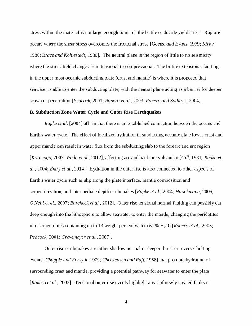
A. The Outer Rise and Plate Stress Field

[Supak et al., 2006] [Garcia- Castellanos et al., 2000]

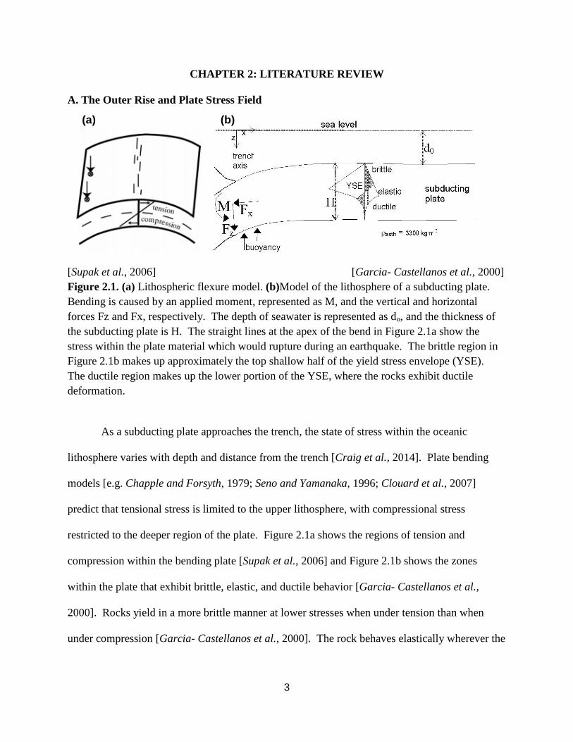
Figure 2.1. (a) Lithospheric flexure model. (b)Model of the lithosphere of a subducting plate.

Bending is caused by an applied moment, represented as M, and the vertical and horizontal

forces Fz and Fx, respectively. The depth of seawater is represented as do, and the thickness of

the subducting plate is H. The straight lines at the apex of the bend in Figure 2.1a show the

stress within the plate material which would rupture during an earthquake. The brittle region in

Figure 2.1b makes up approximately the top shallow half of the yield stress envelope (YSE).

The ductile region makes up the lower portion of the YSE, where the rocks exhibit ductile

deformation.

As a subducting plate approaches the trench, the state of stress within the oceanic

lithosphere varies with depth and distance from the trench [Craig et al., 2014]. Plate bending

models [e.g. Chapple and Forsyth, 1979; Seno and Yamanaka, 1996; Clouard et al., 2007]

predict that tensional stress is limited to the upper lithosphere, with compressional stress

restricted to the deeper region of the plate. Figure 2.1a shows the regions of tension and

compression within the bending plate [Supak et al., 2006] and Figure 2.1b shows the zones

within the plate that exhibit brittle, elastic, and ductile behavior [Garcia- Castellanos et al.,

2000]. Rocks yield in a more brittle manner at lower stresses when under tension than when

under compression [Garcia- Castellanos et al., 2000]. The rock behaves elastically wherever the

(b) (a)

4

stress within the material is not large enough to match the brittle or ductile yield stress. Rupture

occurs where the shear stress overcomes the frictional stress [Goetze and Evans, 1979; Kirby,

1980; Brace and Kohlestedt, 1980]. The neutral plane is the region of little to no seismicity

where the stress field changes from tensional to compressional. The brittle extensional faulting

in the upper most oceanic subducting plate (crust and mantle) is where it is proposed that

seawater is able to enter the subducting plate, with the neutral plane acting as a barrier for deeper

seawater penetration [Peacock, 2001; Ranero et al., 2003; Ranero and Sallares, 2004].

B. Subduction Zone Water Cycle and Outer Rise Earthquakes

Rüpke et al. [2004] affirm that there is an established connection between the oceans and

Earth's water cycle. The effect of localized hydration in subducting oceanic plate lower crust and

upper mantle can result in water flux from the subducting slab to the forearc and arc region

[Korenaga, 2007; Wada et al., 2012], affecting arc and back-arc volcanism [Gill, 1981; Rüpke et

al., 2004; Emry et al., 2014]. Hydration in the outer rise is also connected to other aspects of

Earth's water cycle such as slip along the plate interface, mantle composition and

serpentinization, and intermediate depth earthquakes [Rüpke et al., 2004; Hirschmann, 2006;

O'Neill et al., 2007; Barcheck et al., 2012]. Outer rise tensional normal faulting can possibly cut

deep enough into the lithosphere to allow seawater to enter the mantle, changing the peridotites

into serpentinites containing up to 13 weight percent water (wt % H2O) [Ranero et al., 2003;

Peacock, 2001; Grevemeyer et al., 2007].

Outer rise earthquakes are either shallow normal or deeper thrust or reverse faulting

events [Chapple and Forsyth, 1979; Christensen and Ruff, 1988] that promote hydration of

surrounding crust and mantle, providing a potential pathway for seawater to enter the plate

[Ranero et al., 2003]. Tensional outer rise events highlight areas of newly created faults or

5

reactivated faults, and the infiltration of water in the upper lithosphere of the plate [Ranero et al.,

2003; Moscoso and Contreras-Reyes, 2012]. The neutral plane between tensional seismicity in

the upper layers of the plate and compressional seismicity in the lower portion of the plate is

possibly a barrier for seawater penetration and the limit of serpentinization [Lefeldt et al., 2009].

Compressional earthquakes occur beneath the neutral plane and are attributed to the

compressional bending stresses or in-plane loading caused by plate coupling [Chapple and

Forsyth, 1979; Christensen and Ruff, 1988]. Compressional events occur in much fewer

numbers and at deeper depths than tensional earthquakes in the outer rise.

Lefeldt et al. [2009] suggest that outer rise events larger than Mw=5 might create faults

that may allow sea water to penetrate the plate down to depths of the earthquake origin. There

are numerous events larger than Mw=5 that occur in the outer rise in Colombia, Ecuador, Peru,

and Chile, which perhaps contribute to seismicity at deeper depths, bending related faults, and

more hydration in the subducting plate than previous studies have predicted [Van Avendonk et

al., 2011].

Other than high lithostatic pressure, it is not certain how or by what process water is

pulled to depth. However, some studies suggest that plate bending causes tectonic pressure

gradients within the upper oceanic lithosphere that pull water into the mantle [Faccenda et al.,

2009; Emry et al., 2014]. If serpentinization occurs along outer rise faults, then the amount of

water within the oceanic plate mantle is possibly equal to the amount of water stored within the

oceanic crust [Ranero et al., 2003; Emry et al., 2014].

The Earth's water cycle consists of the hydration and dehydration of subducting oceanic

lithosphere. Water is chemically bound within the incoming plate’s sedimentary, crustal, and

mantle portions [Rüpke et al., 2004]. The shallowest dehydration is < 20 km depth and consists

6

of expelled water from pore and structurally-bound water in subducting sediments [Jarrard,

2003; Rüpke et al., 2004; Emry et al., 2011]. Water expelled within the upper crustal layer

down to 50 km depth is the stage of the water cycle that may affect plate interface slip and other

shallow subduction zone processes [ Jarrard, 2003; Shelly et al., 2006; Audet et al., 2009; Emry

et al., 2014]. In intermediate depth dehydration (50 - 100 km), water expels from the lower

crustal layer and upper mantle serpentinites [Jarrard, 2003; Van Keken et al., 2011] and affects

volcanic arc output and back arc basin output [Gill, 1981; Kelley et al., 2006]. At depths down

to 100 km, the de-serpentinization of the mantle triggers arc melting [Rüpke et al., 2004].

Hydration in the outer rise has been suggested to occur more commonly in subduction

zones with relatively fast convergence and brittle subducting oceanic crust [van Keken et al.,

2011]. Emry et al. [2014] observed that the maximum centroid depth of tensional earthquakes

in the central Marianas was on the order of 11 km below the Moho, which agreed with models of

serpentinized mantle depth. Such a model as that of Emry et al. [2014] suggests that the overall

hydration in the Marianas is much greater than other models have predicted. The Mariana

subduction zone, like the Nazca subduction zone, is a highly coupled region with relatively fast

subduction. However, in contrast to the old (~170 million years), thick, and cold Pacific plate in

the Mariana subduction zone, the Nazca plate has relatively young oceanic lithosphere (~ 20 - 40

million years) and subduction dip varies between 9 -30° along the length of the plate [Gutscher

et al., 2000; Garcia et. al., 2007]. Thus, we expect the depth of tensional faulting and hydration

in the Nazca outer rise to be more shallow than in the Marianas outer rise.

7

C. Structure of the Nazca Plate Offshore South America

The state of stress and hydration is not well constrained for the Nazca - South American

plate subduction zone, specifically offshore Colombia and the 4,270 km extent of offshore Chile.

The convergence rate of the Nazca plate with South America also changes throughout this

subduction zone, increasing from 6.0 cm/yr at ~ 5°N to 7.0 cm/yr at ~ 5°S to 7.8 cm/yr at ~ 15°S

to 8.4 cm/yr at ~ 30°S [Gutscher et al., 2000]. There is no linear relationship between latitude

and the age of plate. Gutscher et al. [2000] estimated that the age of the subducting Nazca plate

varies from ~ 22 Ma, 12 Ma, 43 Ma, and 6 Ma [Tilmann et al., 2008] at 7°N, 4.5°N, 24°S-31°S,

and 41°S, respectively. There are multiple fracture zones (oblique and perpendicular to the

trench), multiple transform faults, the Sandra rift (no longer spreading) perpendicular to the

trench, as well as the Carnegie, Nazca, Iquique, and Juan-Fernandez ridges [Gutscher et al.,

2002]. Pre-existing fractures associated with features in the bathymetry (such as ridges and

seamounts) could be a controlling factor in the nucleation of outer rise seismicity [Fromm et al.,

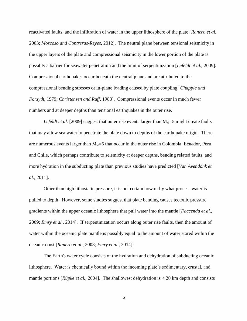
2006]. As seen in Figure 2.2, there are large concentrations of outer rise normal faulting events

in the Colombia and Chile regions (8°N - 0°N and 22°S - 46°S). Additionally there are regions

with lower rates of earthquakes along the margin (0°N - 5°S and 12°S - 25°S).

The seafloor structure is unusual in the northern part of the study region of 8°N - 0 °N.

From 5.6°N - 7°N, the subduction is characterized by shallow, flat- slab subduction of the

Panama Basin, with no volcanic arc [Gutscher et al., 2000]. The presence of volcanic arcs

affirm that there is water in the Nazca plate. There is a volcanic gap from 2°S - 15°S, possibly

due to flat slab subduction [Gutscher et al., 2000].

At 15°S latitude and farther south to 45° S, the character of subduction changes, with a

steep subduction angle and the presence of a volcanic arc [Gutscher et al., 2000]. The

8

concentration of normal faulting outer rise events in Chile correlates with regions seaward of

rupture from the 1960 Mw=9.5 Valdivia and 2010 Mw=8.8 Maule megathrust earthquakes [Craig

et al., 2014]. As a result, this study will concentrate on these areas along the 1960 and 2010

rupture areas.

Figure 2.2 also displays the areas of volcanic arcs (8°N - 2°S, 15°S - 27°S, and

32°S - 46°S) and gaps (5°S - 15°S and 27°S - 32°S) along the margin of the Nazca plate. These

volcanic arcs and gaps could possibly be related to plate hydration in the outer rise because of

water’s effect to lower the mantle melting temperature [Gutscher et al., 2000; Emry et al., 2011].

In the Chile subduction zone near 32°S, the outer rise seismicity may be influenced by the

complex fault system created by the subduction of the Juan Fernandez Ridge [Clouard et al.,

2007; Fromm et. al., 2006].

In the southern portions of South America, extending throughout southern central Chile

(41-44°S), the plate is older (15-25 Ma) and therefore relatively colder and more rigid than

younger portions of the plate. There is approximately 9 hydrated (serpentinized) lithosphere

in the upper 2 km of the Nazca plate [Contreras -Reyes, 2007], but hydration and dehydration of

the subduction zone of Colombia is not well known or investigated [van Keken et al., 2011].

9

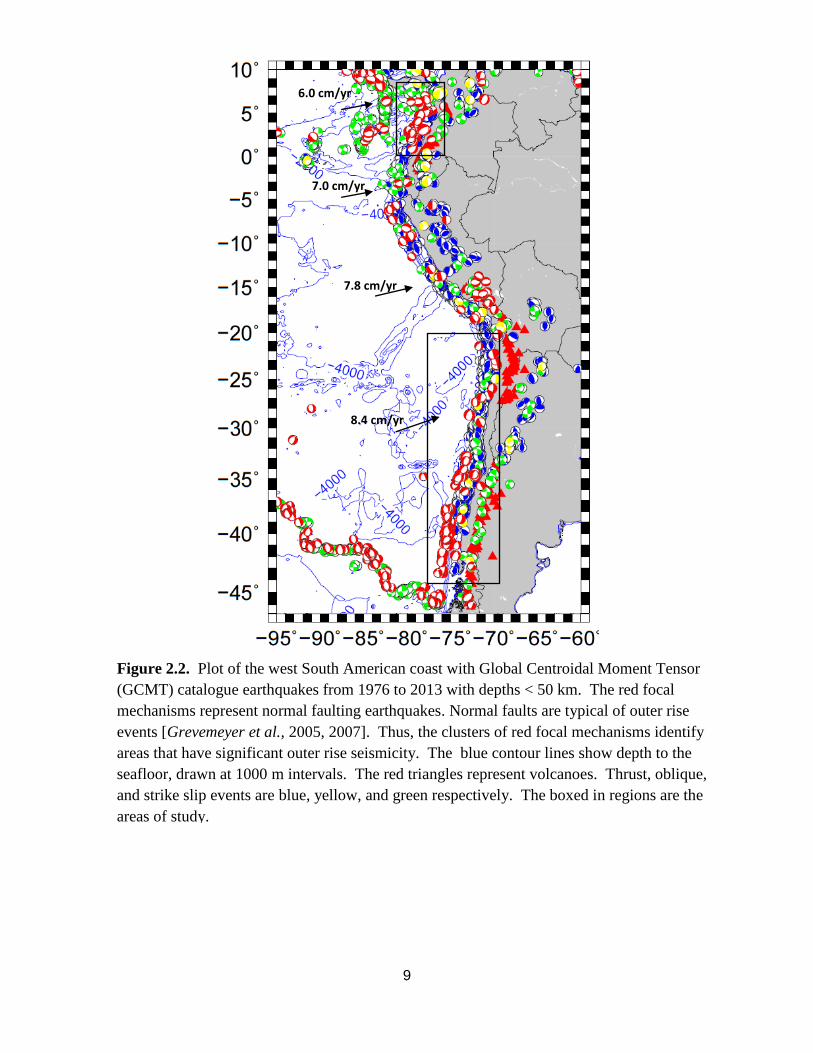
Figure 2.2. Plot of the west South American coast with Global Centroidal Moment Tensor

(GCMT) catalogue earthquakes from 1976 to 2013 with depths < 50 km. The red focal

mechanisms represent normal faulting earthquakes. Normal faults are typical of outer rise

events [Grevemeyer et al., 2005, 2007]. Thus, the clusters of red focal mechanisms identify

areas that have significant outer rise seismicity. The blue contour lines show depth to the

seafloor, drawn at 1000 m intervals. The red triangles represent volcanoes. Thrust, oblique,

and strike slip events are blue, yellow, and green respectively. The boxed in regions are the

areas of study.

6.0 cm/yr

7.0 cm/yr

8.4 cm/yr

7.8 cm/yr

10

D. Previous Studies of the Nazca Plate Outer Rise

In previous studies, the subducting mantle off the coast of Nicaragua (north of this

paper's study area) is suggested to be about 20 - 30 serpentinized. Lefeldt et al. [2009] inferred

the depth of the neutral plane in the Nicaraguan outer rise from earthquake focal mechanisms

and found that it corresponded to a region of low P-wave velocities, characteristic of mantle

serpentinization. In the Nicaraguan outer rise, serpentinization occurs down to a depth of

5 - 10 km with plate hydration of 3 - 4 wt % H2O [Van Avendonk et al., 2011]. The results from

van Keken et al. [2011] suggest that the Colombia and Peru regions have less water input. The

Chile region has similar water input to that of Nicaragua, though the entire region from

Colombia to Chile has much more dehydration, which occurs at ~100 km depth, throughout the

subduction process [Van Avendonk et al., 2011; van Keken et al. 2011].

Both Clouard et al. [2007] and Fromm et al. [2006] studied the 04/09/2001 outer rise

Chile earthquake, which is the largest outer rise event, ( ) [Fromm et al., 2006], to have

occurred since 1993 in the study region. This earthquake was calculated by both studies to have

a source depth of ~12 km. Both concluded that the outer rise earthquake was characterized by

normal faulting, striking sub-parallel to the Juan Fernandez Ridge and could have created faults

that allowed seawater into the plate. Both studies also mention that the nearby O'Higgins

fracture zone and the Juan Fernandez Ridge affect outer rise seismic nucleation [Fromm et al.,

2006; Clouard et al., 2007]. Clouard et al. [2007] inferred that the lithosphere in this region of

Chile is in tension down to a depth of 30 km and Fromm et al. [2006] inferred that brittle failure

occurs from 10 - 30 km depth.

Oceanic intraplate seismicity is confined to regions colder than 600° C [McKenzie et

al.,2005; Craig et al., 2014]. The 600° C isotherm in the Central American outer rise has been

11

inferred to be at 18 - 26 km depth with the deepest extensional earthquake at 10 km and deepest

compressional earthquake at 15 km [Craig et al., 2014], which agrees with the Van Avendonk et

al. [2011] study. The aseismic region corresponding to the 600° C isotherm in the Chile outer

rise has been inferred to be at 15 - 35 km depth, with the deepest extensional and compressional

earthquakes at 23 km and 28 km depths, respectively [Craig et al., 2014]. This would suggest a

neutral plane at 24 - 27 km depth for the Chile outer rise. However, the Craig et al. [2014] study

assumed a uniform curvature structure of the Nazca plate, which in reality has bathymetry and

curvature that varies greatly along the length of the Chile subduction zone.

12

CHAPTER 3: EARTHQUAKE RELOCATION

A. Data and Methods

Uncertainties in automated teleseismic event locations, especially for shallow

earthquakes, can be caused by timing errors, the limitations of the algorithms, or phase pick

errors [Lomax et al., 2000; McGinnis, 2001]. Therefore, relocation is necessary to have accurate

event epicenter locations and to distinguish the outer rise earthquakes from shallow thrust

earthquakes in the forearc of the subduction zone [Emry, 2011]. In this research, we used the

hypocentroidal decomposition method [Jordan and Sverdrup, 1981] to precisely locate outer rise

earthquake epicenters in the study area down to a depth of 50 km. We identified earthquakes

with depths < 50 km and MW 5 for the Colombia region (0°N - 10 °N, 77°W - 83°W) and

MW 5.5 for the Chile region (18°S - 44°S, 72°W - 82°W) from 01/01/1976 to 01/01/2013 in

the Global Centroidal Moment Tensor (GCMT) catalogue [Ekström et al., 2012]. Arrival time

data was collected from the International Seismic Center (ISC) Bulletin, including P, pP, PKP,

and S phases for earthquakes MW 5, for the Colombia and Chile regions. Earthquakes

80 km landward of the trench are excluded. The remaining GCMT earthquakes were

combined with arrival time data for the same events.

The hypocentroidal decomposition algorithm [Jordan and Sverdrup, 1981] was used to

calculate more accurate locations than those reported in the ISC Bulletin. The Jordan and

Sverdrup [1981] method is dependent on the assumption that if the distance between earthquake

hypocenters is small, then the difference in travel times to a station does not include the effects

of velocity heterogeneity [Wolfe, 2002]. This method relocates earthquakes within a cluster with

respect to the cluster centroid by projecting out the part of the travel-time deviations that are

13

common to particular stations [Shearer, 2009]. Earthquake ISC and GCMT earthquake locations

were separated into two regions of Colombia (0°N - 10 °N) and Chile (18°S - 44°S).

B. Results - Colombia

In Colombia, relocation was done in one section since the study region is relatively small,

0 - 10 N, and the ray paths should be similar throughout this section. Of the initial 42 GCMT

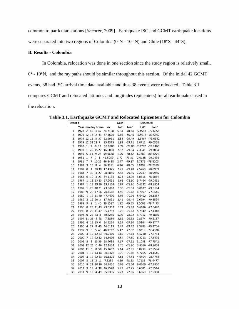
events, 38 had ISC arrival time data available and thus 38 events were relocated. Table 3.1

compares GCMT and relocated latitudes and longitudes (epicenters) for all earthquakes used in

the relocation.

Table 3.1. Earthquake GCMT and Relocated Epicenters for Colombia Event # GCMT Relocated

Year mo day hr mn sec Lat Lon Lat Lon 1 1978 2 16 3 47 24.7158 5.84 -78.24 5.4568 -77.6556 2 1979 12 13 2 43 37.1670 5.66 -80.46 5.5014 -80.5307 3 1979 12 13 5 37 52.9961 2.88 -79.49 2.5467 -79.6342 4 1979 12 31 23 7 25.4375 1.93 -79.71 2.0712 -79.0368 5 1980 1 7 0 33 39.0885 2.74 -79.06 2.8787 -78.7466 6 1980 1 26 15 27 16.0000 2.52 -79.84 2.3341 -79.3804 7 1980 5 11 9 25 59.9688 1.95 -80.32 1.7889 -80.4094 8 1981 1 7 7 1 41.5059 1.72 -79.31 2.0136 -79.2436 9 1981 7 7 10 25 46.8438 2.77 -79.87 2.7373 -79.8203 10 1982 3 16 8 4 56.3281 6.26 -78.65 5.8299 -78.2359 11 1982 8 1 20 38 17.4375 2.71 -79.40 2.5268 -78.8939 12 1984 7 30 4 27 28.6846 2.58 -79.35 2.2749 -78.9946 13 1985 6 10 3 23 34.1133 3.24 -78.99 3.0316 -78.5034 14 1987 1 13 13 23 57.2031 5.68 -78.90 5.7464 -79.0461 15 1987 1 13 19 30 13.7109 5.87 -78.86 5.6232 -78.8854 16 1987 1 25 10 31 23.9883 3.30 -79.31 3.0637 -79.3184 17 1988 9 20 17 56 20.4688 4.99 -77.68 4.7097 -77.3646 18 1989 1 17 11 20 47.4609 5.93 -79.01 5.6492 -79.1387 19 1989 2 12 20 3 17.7891 2.41 -79.44 2.6994 -79.8594 20 1989 9 9 1 40 39.1587 1.92 -79.53 2.5003 -79.7493 21 1990 8 25 11 43 29.0352 5.71 -77.93 5.6696 -77.5470 22 1990 8 25 11 47 35.4297 6.26 -77.63 5.7542 -77.4348 23 1994 9 27 23 4 50.2266 5.90 -78.92 5.7212 -79.1836 24 1994 11 26 4 48 7.5859 2.65 -79.32 2.8374 -79.5167 25 1995 4 13 15 0 34.5234 5.29 -79.80 5.5164 -79.8747 26 1996 4 27 8 40 44.6113 2.47 -79.42 2.3983 -79.3764 27 1997 9 9 5 45 48.9727 5.47 -77.82 5.8313 -77.4338 28 2000 3 19 12 23 39.7109 5.69 -77.61 5.6210 -77.5754 29 2000 7 12 22 12 14.8906 6.54 -77.80 6.2713 -77.6495 30 2002 8 8 13 39 58.9688 5.17 -77.62 5.1058 -77.7542 31 2002 12 21 0 46 12.1624 3.76 -78.90 3.8016 -78.9008 32 2003 11 5 0 58 45.1602 5.14 -77.81 5.0239 -77.5594 33 2004 1 12 14 14 30.6328 5.76 -79.08 5.7205 -79.1646 34 2007 3 17 22 43 10.1875 4.61 -78.53 4.6504 -78.4788 35 2007 3 18 2 11 7.5259 4.69 -78.53 4.7135 -78.4477 35 2010 8 21 20 20 16.7656 6.08 -78.04 6.0669 -77.9800 37 2011 9 13 4 38 46.9570 5.77 -77.75 5.6601 -77.5544 38 2011 9 13 4 49 35.9395 5.73 -77.66 5.6660 -77.5358

14

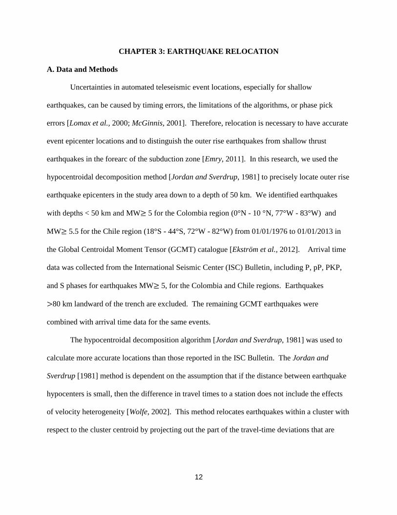
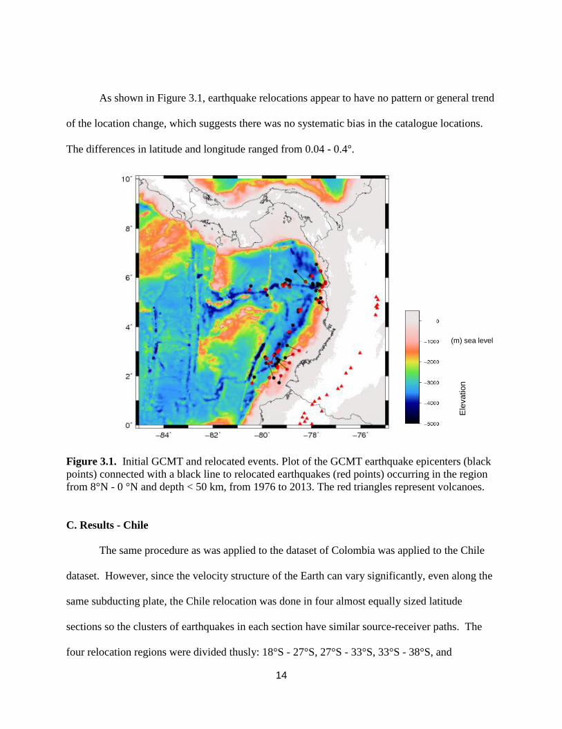
As shown in Figure 3.1, earthquake relocations appear to have no pattern or general trend

of the location change, which suggests there was no systematic bias in the catalogue locations.

The differences in latitude and longitude ranged from 0.04 - 0.4 .

Figure 3.1. Initial GCMT and relocated events. Plot of the GCMT earthquake epicenters (black

points) connected with a black line to relocated earthquakes (red points) occurring in the region

from 8°N - 0 °N and depth < 50 km, from 1976 to 2013. The red triangles represent volcanoes.

C. Results - Chile

The same procedure as was applied to the dataset of Colombia was applied to the Chile

dataset. However, since the velocity structure of the Earth can vary significantly, even along the

same subducting plate, the Chile relocation was done in four almost equally sized latitude

sections so the clusters of earthquakes in each section have similar source-receiver paths. The

four relocation regions were divided thusly: 18°S - 27°S, 27°S - 33°S, 33°S - 38°S, and

(m) sea level

Ele

vatio

n

15

38°S - 44°S. Note that the two northernmost of these regions had few earthquakes. Thus,

earthquakes occurring > 80 km seaward of the trench were included, and the earthquakes from

section 2 were combined with section 1 in order to have at least 15 events for each relocation

section. The sections that relocation was done are shown in white boxes in Figure 3.2. Of the

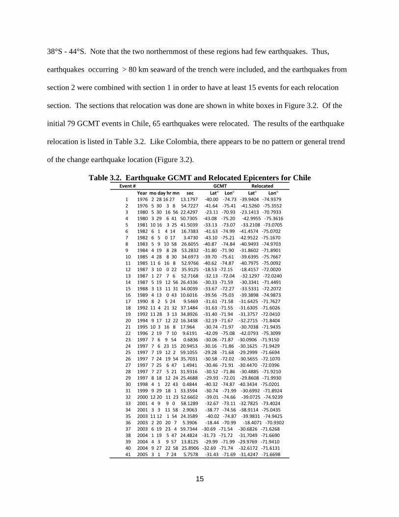
initial 79 GCMT events in Chile, 65 earthquakes were relocated. The results of the earthquake

relocation is listed in Table 3.2. Like Colombia, there appears to be no pattern or general trend

of the change earthquake location (Figure 3.2).

Table 3.2. Earthquake GCMT and Relocated Epicenters for Chile Event # GCMT Relocated

Year mo day hr mn sec Lat Lon Lat Lon 1 1976 2 28 16 27 13.1797 -40.00 -74.73 -39.9404 -74.9379 2 1976 5 30 3 8 54.7227 -41.64 -75.41 -41.5260 -75.3552 3 1980 5 30 16 56 22.4297 -23.11 -70.93 -23.1413 -70.7933 4 1980 3 29 6 41 50.7305 -43.08 -75.20 -42.9955 -75.3616 5 1981 10 16 3 25 41.5039 -33.13 -73.07 -33.2108 -73.0705 6 1982 6 1 4 14 16.7383 -41.63 -74.99 -41.4574 -75.0702 7 1982 6 5 0 17 3.4730 -43.10 -75.21 -42.9522 -75.1670 8 1983 5 9 10 58 26.6055 -40.87 -74.84 -40.9493 -74.9703 9 1984 4 19 8 28 53.2832 -31.80 -71.90 -31.8602 -71.8901 10 1985 4 28 8 30 34.6973 -39.70 -75.61 -39.6395 -75.7667 11 1985 11 6 16 8 52.9766 -40.62 -74.87 -40.7975 -75.0092 12 1987 3 10 0 22 35.9125 -18.53 -72.15 -18.4157 -72.0020 13 1987 1 27 7 6 52.7168 -32.13 -72.04 -32.1297 -72.0240 14 1987 5 19 12 56 26.4336 -30.33 -71.59 -30.3341 -71.4491 15 1988 3 13 11 31 34.0039 -33.67 -72.27 -33.5331 -72.2072 16 1989 4 13 0 43 10.6016 -39.56 -75.03 -39.3898 -74.9873 17 1990 8 2 5 24 9.5469 -31.61 -71.58 -31.6425 -71.7627 18 1992 11 4 21 32 37.1484 -31.63 -71.55 -31.6305 -71.6026 19 1992 11 28 3 13 34.8926 -31.40 -71.94 -31.3757 -72.0410 20 1994 9 17 12 22 16.3438 -32.19 -71.67 -32.2715 -71.8404 21 1995 10 3 16 8 17.964 -30.74 -71.97 -30.7038 -71.9435 22 1996 2 19 7 10 9.6191 -42.09 -75.08 -42.0793 -75.3099 23 1997 7 6 9 54 0.6836 -30.06 -71.87 -30.0906 -71.9150 24 1997 7 6 23 15 20.9453 -30.16 -71.86 -30.1625 -71.9429 25 1997 7 19 12 2 59.1055 -29.28 -71.68 -29.2999 -71.6694 26 1997 7 24 19 54 35.7031 -30.58 -72.02 -30.5655 -72.1070 27 1997 7 25 6 47 1.4941 -30.46 -71.91 -30.4470 -72.0396 28 1997 7 27 5 21 31.9316 -30.52 -71.86 -30.4885 -71.9210 29 1997 8 18 12 24 25.4688 -29.93 -72.01 -29.8608 -71.9930 30 1998 4 1 22 43 0.4844 -40.32 -74.87 -40.3434 -75.0201 31 1999 9 29 18 1 33.3594 -30.74 -71.99 -30.6992 -71.8924 32 2000 12 20 11 23 52.6602 -39.01 -74.66 -39.0725 -74.9239 33 2001 4 9 9 0 58.1289 -32.67 -73.11 -32.7825 -73.4024 34 2001 3 3 11 58 2.9063 -38.77 -74.56 -38.9114 -75.0435 35 2003 11 12 1 54 24.3589 -40.02 -74.87 -39.9831 -74.9425 36 2003 2 20 20 7 5.3906 -18.44 -70.99 -18.4071 -70.9302 37 2003 6 19 23 4 59.7344 -30.69 -71.54 -30.6826 -71.6268 38 2004 1 19 5 47 24.4824 -31.73 -71.72 -31.7049 -71.6690 39 2004 4 3 9 57 13.8125 -29.99 -71.99 -29.9769 -71.9410 40 2004 9 27 22 58 25.8906 -32.69 -71.74 -32.6172 -71.6131 41 2005 3 1 7 24 5.7578 -31.43 -71.69 -31.4247 -71.6698

16

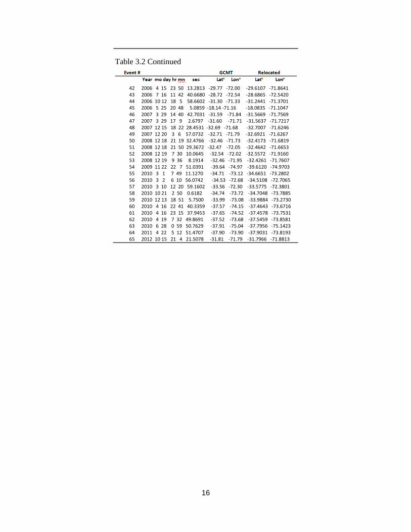
Table 3.2 Continued

42 2006 4 15 23 50 13.2813 -29.77 -72.00 -29.6107 -71.8641 43 2006 7 16 11 42 40.6680 -28.72 -72.54 -28.6865 -72.5420 44 2006 10 12 18 5 58.6602 -31.30 -71.33 -31.2441 -71.3701 45 2006 5 25 20 48 5.0859 -18.14 -71.16 -18.0835 -71.1047 46 2007 3 29 14 40 42.7031 -31.59 -71.84 -31.5669 -71.7569 47 2007 3 29 17 9 2.6797 -31.60 -71.71 -31.5637 -71.7217 48 2007 12 15 18 22 28.4531 -32.69 -71.68 -32.7007 -71.6246 49 2007 12 20 3 6 57.0732 -32.71 -71.79 -32.6921 -71.6267 50 2008 12 18 21 19 32.4766 -32.46 -71.73 -32.4173 -71.6819 51 2008 12 18 21 50 29.3672 -32.47 -72.05 -32.4642 -71.6653 52 2008 12 19 7 30 10.0645 -32.54 -72.02 -32.5572 -71.9160 53 2008 12 19 9 36 8.1914 -32.46 -71.95 -32.4261 -71.7607 54 2009 11 22 22 7 51.0391 -39.64 -74.97 -39.6120 -74.9703 55 2010 3 1 7 49 11.1270 -34.71 -73.12 -34.6651 -73.2802 56 2010 3 2 6 10 56.0742 -34.53 -72.68 -34.5108 -72.7065 57 2010 3 10 12 20 59.1602 -33.56 -72.30 -33.5775 -72.3801 58 2010 10 21 2 50 0.6182 -34.74 -73.72 -34.7048 -73.7885 59 2010 12 13 18 51 5.7500 -33.99 -73.08 -33.9884 -73.2730 60 2010 4 16 22 41 40.3359 -37.57 -74.15 -37.4643 -73.6716 61 2010 4 16 23 15 37.9453 -37.65 -74.52 -37.4578 -73.7531 62 2010 4 19 7 32 49.8691 -37.52 -73.68 -37.5459 -73.8581 63 2010 6 28 0 59 50.7629 -37.91 -75.04 -37.7956 -75.1423 64 2011 4 22 5 12 51.4707 -37.90 -73.90 -37.9031 -73.8193 65 2012 10 15 21 4 21.5078 -31.81 -71.79 -31.7966 -71.8813

17

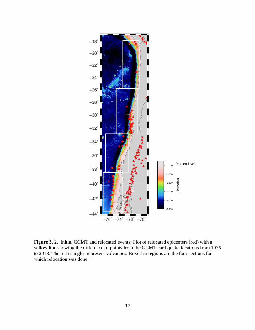
Figure 3. 2. Initial GCMT and relocated events: Plot of relocated epicenters (red) with a

yellow line showing the difference of points from the GCMT earthquake locations from 1976

to 2013. The red triangles represent volcanoes. Boxed in regions are the four sections for

which relocation was done.

(m) sea level

Ele

vatio

n

18

CHAPTER 4: WAVEFORM INVERSION

A. Earthquake Selection and Data

The purpose of performing waveform inversion is to determine the best fitting source

parameters for earthquakes located on the incoming plate or near the trench axis. These source

parameters include focal mechanism (strike, dip, slip), magnitude, and point source depth.

Earthquakes occurring in 1993 or later are those with digital teleseismic waveform data

available. The events that have 0 are likely to be more susceptible to error due to the

smaller magnitudes, shallow source depths and therefore less pronounced wave arrivals.

Waveforms were visually inspected for clear signals and teleseismic P-, SH- and SV- waveforms

were inverted from stations at distances 30 95 .

Of the 38 relocated earthquakes in the Colombian region, 11 occurred in 1993 or later

with a moment magnitude larger than 5.50. Additionally, of the 11 events that occurred in 1993

or later with , only two earthquakes are in the outer rise zone seaward of the trench.

These earthquakes are the two largest and most recent events (03/17/07 and 03/18/07,

6.00 and 6.40, respectively). Since there were only two earthquakes in the Colombia

region that fit the parameters for waveform inversion, the outer rise events of 11/26/94 and

12/21/2002, both with , were included in the waveform inversion. Of the relocated

earthquakes in the Chile region, 16 occurred in 1993 or later with 5.50. Of these 16, 10

were normal faulting events in the outer rise. The relocated events that were used for waveform

inversion are plotted for both the Chile and Colombia regions in Figure 4.1.

19

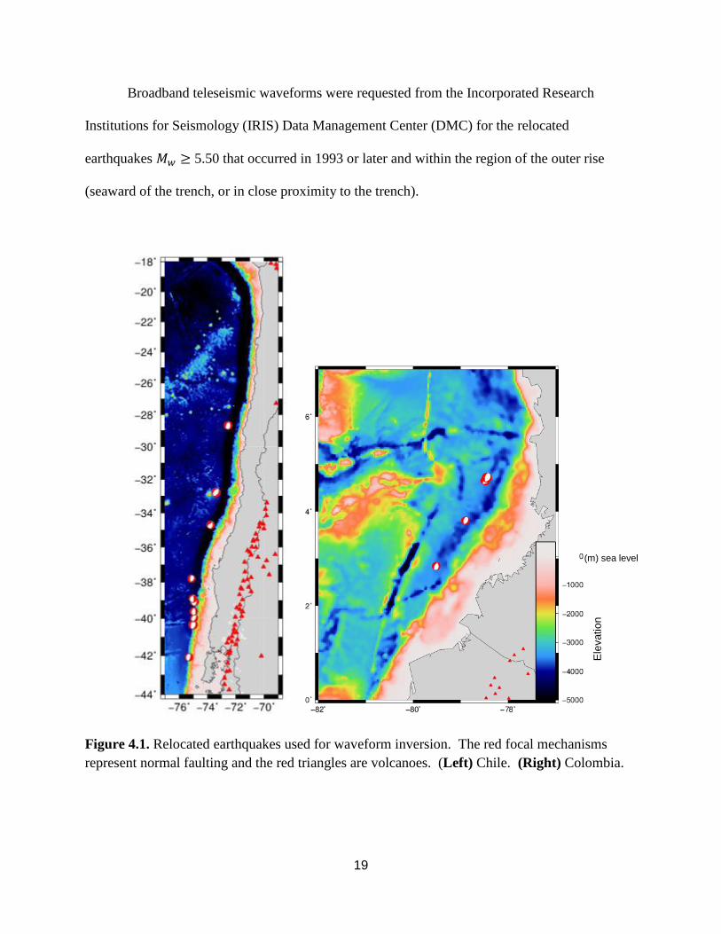
Broadband teleseismic waveforms were requested from the Incorporated Research

Institutions for Seismology (IRIS) Data Management Center (DMC) for the relocated

earthquakes 5.50 that occurred in 1993 or later and within the region of the outer rise

(seaward of the trench, or in close proximity to the trench).

Figure 4.1. Relocated earthquakes used for waveform inversion. The red focal mechanisms

represent normal faulting and the red triangles are volcanoes. (Left) Chile. (Right) Colombia.

(m) sea level

Ele

vatio

n

20

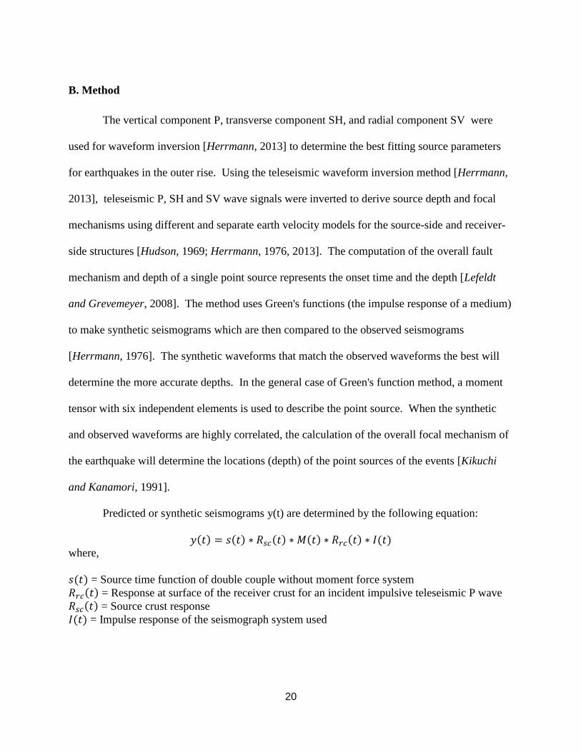
B. Method

The vertical component P, transverse component SH, and radial component SV were

used for waveform inversion [Herrmann, 2013] to determine the best fitting source parameters

for earthquakes in the outer rise. Using the teleseismic waveform inversion method [Herrmann,

2013], teleseismic P, SH and SV wave signals were inverted to derive source depth and focal

mechanisms using different and separate earth velocity models for the source-side and receiver-

side structures [Hudson, 1969; Herrmann, 1976, 2013]. The computation of the overall fault

mechanism and depth of a single point source represents the onset time and the depth [Lefeldt

and Grevemeyer, 2008]. The method uses Green's functions (the impulse response of a medium)

to make synthetic seismograms which are then compared to the observed seismograms

[Herrmann, 1976]. The synthetic waveforms that match the observed waveforms the best will

determine the more accurate depths. In the general case of Green's function method, a moment

tensor with six independent elements is used to describe the point source. When the synthetic

and observed waveforms are highly correlated, the calculation of the overall focal mechanism of

the earthquake will determine the locations (depth) of the point sources of the events [Kikuchi

and Kanamori, 1991].

Predicted or synthetic seismograms y(t) are determined by the following equation:

where,

= Source time function of double couple without moment force system

= Response at surface of the receiver crust for an incident impulsive teleseismic P wave

= Source crust response

= Impulse response of the seismograph system used

21

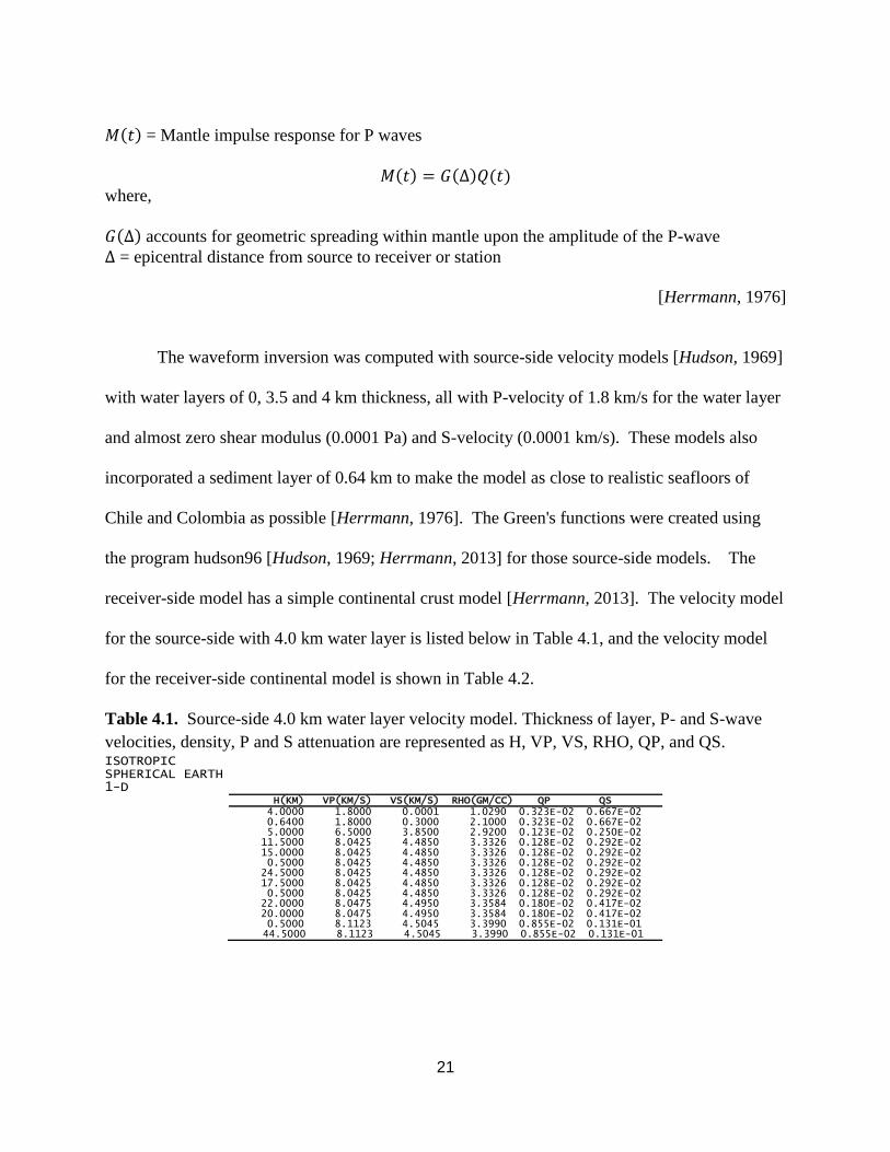
= Mantle impulse response for P waves

where,

accounts for geometric spreading within mantle upon the amplitude of the P-wave

= epicentral distance from source to receiver or station

[Herrmann, 1976]

The waveform inversion was computed with source-side velocity models [Hudson, 1969]

with water layers of 0, 3.5 and 4 km thickness, all with P-velocity of 1.8 km/s for the water layer

and almost zero shear modulus (0.0001 Pa) and S-velocity (0.0001 km/s). These models also

incorporated a sediment layer of 0.64 km to make the model as close to realistic seafloors of

Chile and Colombia as possible [Herrmann, 1976]. The Green's functions were created using

the program hudson96 [Hudson, 1969; Herrmann, 2013] for those source-side models. The

receiver-side model has a simple continental crust model [Herrmann, 2013]. The velocity model

for the source-side with 4.0 km water layer is listed below in Table 4.1, and the velocity model

for the receiver-side continental model is shown in Table 4.2.

Table 4.1. Source-side 4.0 km water layer velocity model. Thickness of layer, P- and S-wave

velocities, density, P and S attenuation are represented as H, VP, VS, RHO, QP, and QS. ISOTROPIC SPHERICAL EARTH 1-D

H(KM) VP(KM/S) VS(KM/S) RHO(GM/CC) QP QS 4.0000 1.8000 0.0001 1.0290 0.323E-02 0.667E-02 0.6400 1.8000 0.3000 2.1000 0.323E-02 0.667E-02 5.0000 6.5000 3.8500 2.9200 0.123E-02 0.250E-02 11.5000 8.0425 4.4850 3.3326 0.128E-02 0.292E-02 15.0000 8.0425 4.4850 3.3326 0.128E-02 0.292E-02 0.5000 8.0425 4.4850 3.3326 0.128E-02 0.292E-02 24.5000 8.0425 4.4850 3.3326 0.128E-02 0.292E-02 17.5000 8.0425 4.4850 3.3326 0.128E-02 0.292E-02 0.5000 8.0425 4.4850 3.3326 0.128E-02 0.292E-02 22.0000 8.0475 4.4950 3.3584 0.180E-02 0.417E-02 20.0000 8.0475 4.4950 3.3584 0.180E-02 0.417E-02 0.5000 8.1123 4.5045 3.3990 0.855E-02 0.131E-01 44.5000 8.1123 4.5045 3.3990 0.855E-02 0.131E-01

22

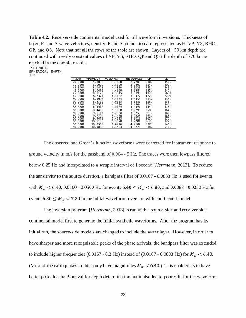
Table 4.2. Receiver-side continental model used for all waveform inversions. Thickness of

layer, P- and S-wave velocities, density, P and S attenuation are represented as H, VP, VS, RHO,

QP, and QS. Note that not all the rows of the table are shown. Layers of ~50 km depth are

continued with nearly constant values of VP, VS, RHO, QP and QS till a depth of 770 km is

reached in the complete table. ISOTROPIC SPHERICAL EARTH 1-D

The observed and Green’s function waveforms were corrected for instrument response to

ground velocity in m/s for the passband of 0.004 - 5 Hz. The traces were then lowpass filtered

below 0.25 Hz and interpolated to a sample interval of 1 second [Herrmann, 2013]. To reduce

the sensitivity to the source duration, a bandpass filter of 0.0167 - 0.0833 Hz is used for events

with , 0.0100 - 0.0500 Hz for events , and 0.0083 - 0.0250 Hz for

events in the initial waveform inversion with continental model.

The inversion program [Herrmann, 2013] is run with a source-side and receiver side

continental model first to generate the initial synthetic waveforms. After the program has its

initial run, the source-side models are changed to include the water layer. However, in order to

have sharper and more recognizable peaks of the phase arrivals, the bandpass filter was extended

to include higher frequencies (0.0167 - 0.2 Hz) instead of (0.0167 - 0.0833 Hz) for .

(Most of the earthquakes in this study have magnitudes .) This enabled us to have

better picks for the P-arrival for depth determination but it also led to poorer fit for the waveform

H(KM) VP(KM/S) VS(KM/S) RHO(GM/CC) QP QS 20.0000 5.8000 3.4600 2.7200 310. 150. 15.0000 6.5000 3.8500 2.9200 814. 400. 42.5000 8.0425 4.4850 3.3326 783. 343. 42.5000 8.0475 4.4950 3.3584 555. 240. 45.0000 8.1123 4.5045 3.3990 117. 76.3 45.0000 8.2374 4.5137 3.3477 122. 77.9 50.0000 8.3905 4.5634 3.3453 213. 135. 50.0000 8.5726 4.6525 3.3886 218. 138. 50.0000 8.7553 4.7394 3.4344 224. 141. 50.0000 8.9380 4.8263 3.4822 231. 145. 50.0000 9.4433 5.1330 3.9295 259. 164. 50.0000 9.6114 5.2388 3.9253 261. 166. 50.0000 9.7794 5.3450 3.9225 263. 168. 50.0000 9.9473 5.4513 3.9212 265. 170. 50.0000 10.1153 5.5570 3.9204 267. 172. 50.0000 10.8562 6.0246 4.2687 837. 546. 50.0000 10.9883 6.1493 4.3275 818. 541.

23

inversion compared to the continental crust source model. The worse fit is most likely due not

only to the higher frequencies but also from using a source-side model with water table, which

has the effect of reverberations directly following the P-arrival [Herrmann, 1976].

Crustal inhomogeneities such as a water layer can cause complex scattering effects in the

seismic record, making it difficult to determine focal depth. In order to further constrain the

depth and check the depth calculated by the waveform inversion, teleseismic P-wave synthetics

from the waveform inversion were used for stations with good signal-to-noise ratios and clear P-

wave arrivals. The source parameters inputted are seismic moment, focal depth, strike, dip, rake,

and event duration of the triangular shaped source time function [Herrmann, 1976]. The

observed P-wave signal was plotted with and compared to synthetic waveforms for various focal

depths (5-25 km). The best depth was determined by observation and comparison of the arrival

times and duration for each depth between the observed and synthetic waveforms. Features that

we were looking for were similarities between the observed and synthetic waveforms, including

duration, arrival times, and amplitude. By using this method, we were able to constrain a small

range of depths for an event.

C. Results

Waveform inversion using source-side models with 3.0, 3.5, and 4.0 km water layers.

Local water thickness determined which model would be used to make the synthetics. P-wave

depth estimation was done for 14 outer rise earthquakes. 4 of those 14 events were in the

Colombia outer rise and 10 were located in the Chile outer rise. For the Colombian earthquakes,

the 3.5 km water layer velocity model gave the best fit and for the most of the Chilean

earthquakes the 4.0 km water layer velocity model gave the best fit. The Chilean events of

03/03/01 and 04/09/01 had the best fits with the 3.5 km and 4.0 km water layer models,

24

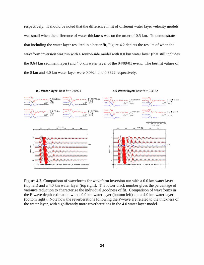
respectively. It should be noted that the difference in fit of different water layer velocity models

was small when the difference of water thickness was on the order of 0.5 km. To demonstrate

that including the water layer resulted in a better fit, Figure 4.2 depicts the results of when the

waveform inversion was run with a source-side model with 0.0 km water layer (that still includes

the 0.64 km sediment layer) and 4.0 km water layer of the 04/09/01 event. The best fit values of

the 0 km and 4.0 km water layer were 0.0924 and 0.3322 respectively.

0.0 Water layer: Best fit = 0.0924 4.0 Water layer: Best fit = 0.3322

Figure 4.2. Comparison of waveforms for waveform inversion run with a 0.0 km water layer

(top left) and a 4.0 km water layer (top right). The lower black number gives the percentage of

variance reduction to characterize the individual goodness of fit. Comparison of waveforms in

the P-wave depth estimation with a 0.0 km water layer (bottom left) and a 4.0 km water layer

(bottom right). Note how the reverberations following the P-wave are related to the thickness of

the water layer, with significantly more reverberations in the 4.0 water layer model.

25

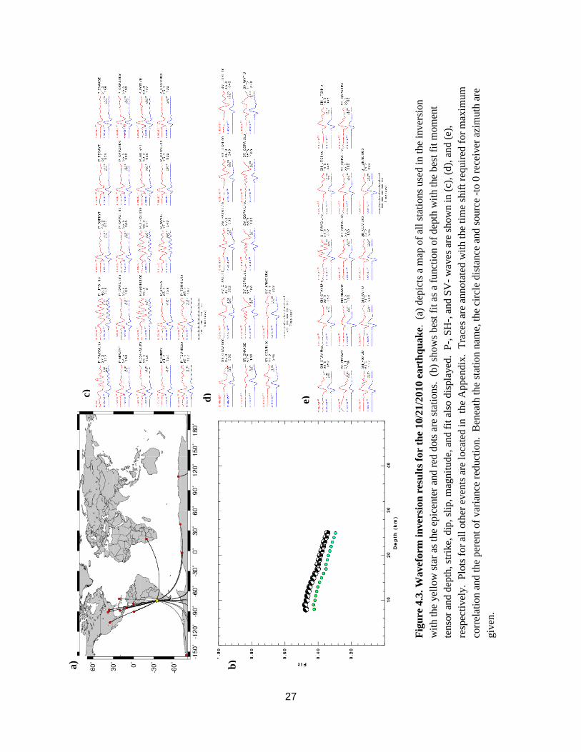
The 10/21/10, 5.93 (GCMT) outer rise earthquake offshore central Chile is the

event used in Figures 4.3 and 4.4. As shown in Figure 4.3a, this earthquake was recorded by 19

stations around the world. These stations are concentrated primarily to the north and south of the

earthquake, with a single station in the east and no stations in the west. For the best fitting depth,

Figure 4.3c-e shows the output of the waveform inversion, where each observed and predicted

component is plotted to the same scale and peak amplitudes. The lower black number gives the

percentage of variance reduction to characterize the individual goodness of fit, where 100%

represents perfect fit [Herrmann, 2013]. The best fit for this earthquake was found to be 0.4391

at 9.0 km depth. The misfit function shown in Figure 4.3 b is peaked at the best depth but is

relatively flat with depth change, as the fit slowly gets smaller with depth. The corresponding

magnitude to the best fit was 5.9 with a strike, dip and rake of 235, 70 and -55. The focal

mechanisms change with depth (Figure 4.3b) from a normal faulting with some strike slip

component at shallow depths to strike slip at deeper depths, > 18 km.

Since the misfit function is relatively flat, displaying the small difference in fit with

depth, we wanted to check the depth calculation. Therefore we compared waveforms with good

signal to noise ratios (observed and picked from Figure 4.3 c) with the synthetic waveforms for

different source depths. The synthetics are computed with the focal mechanism and magnitude

found in the previous step, of 5.85, strike, dip, and slip of 235, 70, -55, and duration of

3.1 s. For all depth estimations, stations with a varied distribution of azimuths were chosen

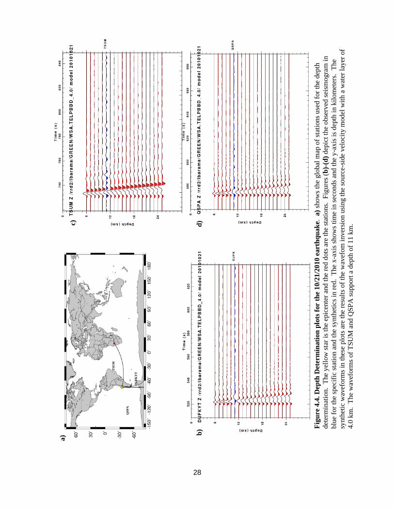
when possible (Figure 4.4a). For this earthquake, we used stations TSUM, DUFKYT, and

QSPA, distributed east, southwest and south of the event (Figure 4.4a). Duration and arrival

times were the features that influenced depth estimations. By plotting the observed waveforms

along with the synthetics, we were able to compare arrival times, durations and amplitudes and

26

observe the effect of the water layer on the waveforms. The synthetic and recorded waveforms

are shown in Figure 4.4b - d, with the preferred depth of 11 km. For these three stations, even

though the peak and trough amplitudes do not have a perfect match, the duration and arrival of

the P-wave appear to support a depth of 11 2 km for the earthquake (Figure 4.4b-d). The

duration of the trough of the initial arrival and peak helped to constrain where the best depth

would be. Additionally, the reverberations after the P-wave are more pronounced for deeper

depths 12-14 km, having three distinct troughs. The shallower waveforms did not really have

this feature. The shape of the peak, particularly in Figure 4.4c, constrains the earthquake to be

no deeper than 14 km depth. Note that station TSUM had the best matching waveform.

27

Fig

ure

4.3

. W

av

efo

rm i

nver

sion

res

ult

s fo

r th

e 10/2

1/2

010

eart

hq

uak

e. (a

) dep

icts

a m

ap o

f al

l st

atio

ns

use

d i

n t

he

inv

ersi

on

wit

h t

he

yel

low

sta

r as

th

e ep

icen

ter

and r

ed d

ots

are

sta

tions.

(b

) sh

ow

s bes

t fi

t as

a f

unct

ion

of

dep

th w

ith

the

bes

t fi

t m

om

ent

ten

sor

and

dep

th, st

rike,

dip

, sl

ip, m

agnit

ude,

and f

it a

lso d

ispla

yed

. P

-, S

H-,

and S

V-

wav

es a

re s

ho

wn

in

(c)

, (d

), a

nd

(e)

,

resp

ecti

vel

y. P

lots

fo

r al

l oth

er e

ven

ts a

re l

oca

ted i

n

the

Appen

dix

. T

race

s ar

e an

nota

ted

wit

h t

he

tim

e sh

ift

req

uir

ed f

or

max

imum

corr

elat

ion

an

d t

he

per

ent

of

var

iance

red

uct

ion.

Ben

eath

the

stat

ion n

ame,

the

circ

le d

ista

nce

and

so

urc

e -t

o 0

rec

eiver

azi

muth

are

giv

en.

a)

b)

c)

d)

e)

28

b)

a)

c)

DU

FK

YT

QS

PA

TS

UM

TS

UM

d)

Fig

ure

4.4

. D

epth

Det

erm

inati

on

plo

ts f

or

the

10/2

1/2

010

eart

hq

uak

e. a)

show

s th

e glo

bal

map

of

stat

ion

s u

sed

for

the

dep

th

det

erm

inat

ion

. T

he

yel

low

sta

r is

the

epic

ente

r an

d t

he

red d

ots

are

the

stat

ions.

F

igure

s (b

)-(d

) d

epic

t th

e o

bse

rved

sei

smo

gra

m i

n

blu

e fo

r th

e sp

ecif

ic s

tati

on

and t

he

synth

etic

s in

red

. T

he

x-a

xis

show

s ti

me

in s

econds

and

the

y-a

xis

is

dep

th i

n k

ilom

eter

s.

The

syn

thet

ic w

avef

orm

s in

thes

e plo

ts a

re t

he

resu

lts

of

the

wav

efom

inver

sion u

sing t

he

sou

rce-

side

vel

oci

ty m

od

el w

ith

a w

ater

lay

er o

f

4.0

km

. T

he

wav

eform

s of

TS

UM

and Q

SP

A s

upport

a d

epth

of

11 k

m.

c)

29

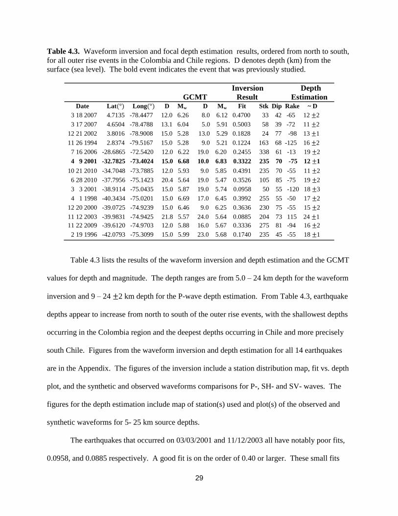
Table 4.3. Waveform inversion and focal depth estimation results, ordered from north to south,

for all outer rise events in the Colombia and Chile regions. D denotes depth (km) from the

surface (sea level). The bold event indicates the event that was previously studied.

Inversion Depth

GCMT Result Estimation Date Lat Long D Mw D Mw Fit Stk Dip Rake ~ D

3 18 2007 4.7135 -78.4477 12.0 6.26 8.0 6.12 0.4700 33 42 -65 12 2

3 17 2007 4.6504 -78.4788 13.1 6.04 5.0 5.91 0.5003 58 39 -72 11 2

12 21 2002 3.8016 -78.9008 15.0 5.28 13.0 5.29 0.1828 24 77 -98 13 1

11 26 1994 2.8374 -79.5167 15.0 5.28 9.0 5.21 0.1224 163 68 -125 16 2

7 16 2006 -28.6865 -72.5420 12.0 6.22 19.0 6.20 0.2455 338 61 -13 19 2

4 9 2001 -32.7825 -73.4024 15.0 6.68 10.0 6.83 0.3322 235 70 -75 12 1

10 21 2010 -34.7048 -73.7885 12.0 5.93 9.0 5.85 0.4391 235 70 -55 11 2

6 28 2010 -37.7956 -75.1423 20.4 5.64 19.0 5.47 0.3526 105 85 -75 19 2

3 3 2001 -38.9114 -75.0435 15.0 5.87 19.0 5.74 0.0958 50 55 -120 18 3

4 1 1998 -40.3434 -75.0201 15.0 6.69 17.0 6.45 0.3992 255 55 -50 17 2

12 20 2000 -39.0725 -74.9239 15.0 6.46 9.0 6.25 0.3636 230 75 -55 15 2

11 12 2003 -39.9831 -74.9425 21.8 5.57 24.0 5.64 0.0885 204 73 115 24 1

11 22 2009 -39.6120 -74.9703 12.0 5.88 16.0 5.67 0.3336 275 81 -94 16 2

2 19 1996 -42.0793 -75.3099 15.0 5.99 23.0 5.68 0.1740 235 45 -55 18 1

Table 4.3 lists the results of the waveform inversion and depth estimation and the GCMT

values for depth and magnitude. The depth ranges are from 5.0 – 24 km depth for the waveform

inversion and 9 – 24 2 km depth for the P-wave depth estimation. From Table 4.3, earthquake

depths appear to increase from north to south of the outer rise events, with the shallowest depths

occurring in the Colombia region and the deepest depths occurring in Chile and more precisely

south Chile. Figures from the waveform inversion and depth estimation for all 14 earthquakes

are in the Appendix. The figures of the inversion include a station distribution map, fit vs. depth

plot, and the synthetic and observed waveforms comparisons for P-, SH- and SV- waves. The

figures for the depth estimation include map of station(s) used and plot(s) of the observed and

synthetic waveforms for 5- 25 km source depths.

The earthquakes that occurred on 03/03/2001 and 11/12/2003 all have notably poor fits,

0.0958, and 0.0885 respectively. A good fit is on the order of 0.40 or larger. These small fits

30

can be attributed to poor quality waveforms with high signal-to-noise ratios. The 2/19/1996,

6/28/2010 and 11/12/2003 events among the deepest earthquakes at 23 km, 19 km, and 24 km

depths respectively. 3/ 3/2001 and 11/12/2003 are also deep, at 19 and 23 km, but unreliable

since waveforms did not have good signal to noise ratio and the fit is low (0.0958 and 0.0885

fits). The events with depth 19 km have reverse normal and thrust faulting mechanisms. Most

of the shallower earthquakes have normal faulting focal mechanisms. The 2010 event is the

most reliable deep earthquake, since it has the best fit of the deeper earthquakes (0.3526 fit).

This event has a source depth of ~19km and shows thrust faulting characteristics from our

calculated moment tensor from the waveform inversion.

The 04/09/2001, 6.68 (GCMT) outer rise earthquake offshore central Chile is the

only event in this study previously studied. We found a focal depth of 10 km with 6.83

from the waveform inversion and 12 1 km with the additional P-wave depth determination

(Appendix). The Fromm et al. [2006] study found the depth of the 04/09/2001 earthquake to be

no greater than 12 km depth, suggesting that rupture could possibly have occurred at depth of 10

to12 km with 6.7. The Clouard et al. [2007] study found a depth of 12 km but with

7.0. Similar to this study, both of these studies used teleseismic waveform inversion and

waveform modeling to determine source depth and focal mechanisms. Additionally, these

studies analyzed the aftershock sequence (through relocation) created by this earthquake. The

range of depths of the aftershocks were from 16 to 46 5 [Clouard et al., 2007]. Our

estimated depths are similar to those of previous studies.

31

CHAPTER 5: DISCUSSION

Many studies have suggested that it is difficult to determine accurate hypocenter depths

of shallow earthquakes occurring near deep sea trenches [e.g., Yoshida et al. 1992; Lefeldt et al.,

2009]. The teleseismic waveform inversion for earthquakes occurring in the study region suffers

from a gap in the distribution of stations in the Pacific and Atlantic Oceans and perhaps the

simplification of a 1-D Earth model. However, we were able to demonstrate that most events in

this region are relatively shallow and have downdip normal mechanisms, typical of outer rise

tensional earthquakes [Lefeldt and Grevemeyer, 2008]. The occurrence of shallow (~ 11- 12 km

depth) events with and the clustering of smaller magnitude outer rise earthquakes in

the southern portion of Chile (32°S - 44°S, refer to Figure 2.2) leads us to infer that there is

potential fluid penetration within the crust and mantle of the subducting Nazca plate in the

Southern Chilean region. Furthermore, the shallower earthquakes in this study had more normal

faulting focal mechanisms, whereas the deeper earthquakes have thrust, reverse normal, and

strike slip characteristics. This difference is consistent with theories that the focal mechanism

will change from normal faulting to thrust faulting as the rupture gets closer to the neutral plane

[Lefeldt and Grevemeyer, 2008].

32

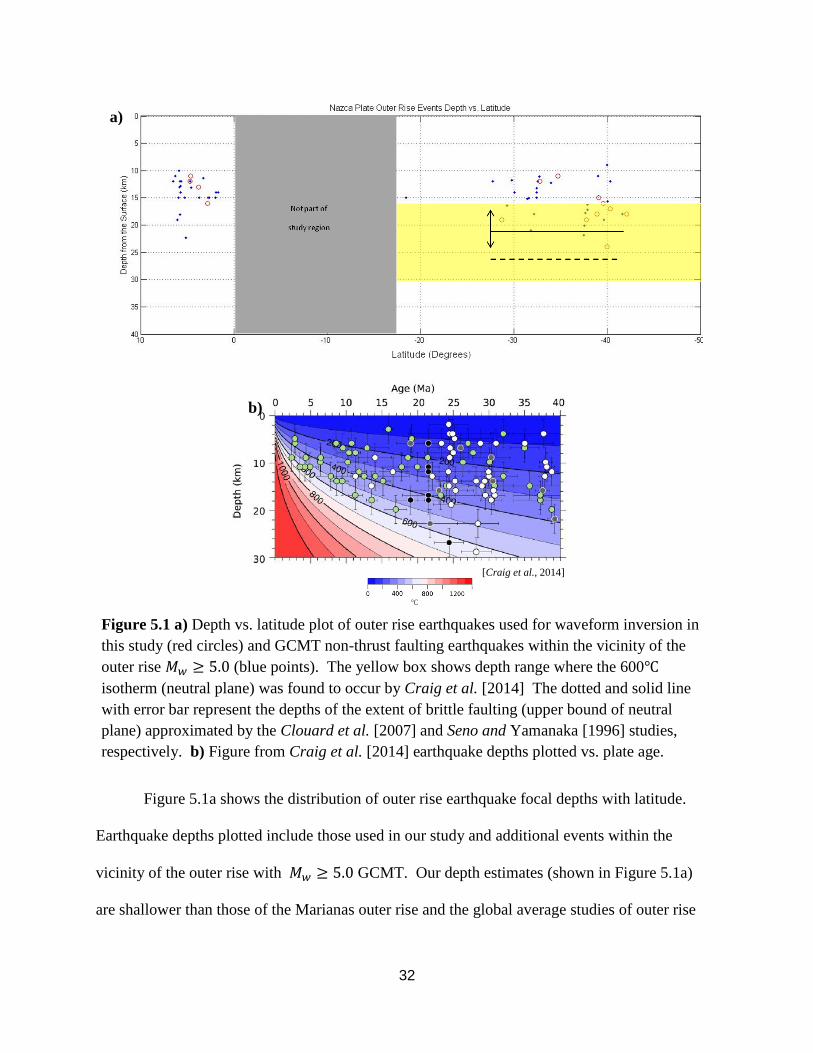
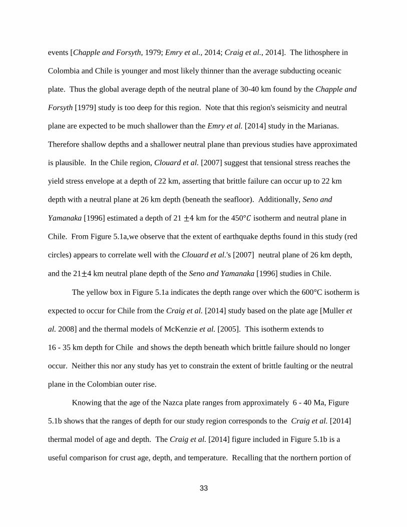
Figure 5.1 a) Depth vs. latitude plot of outer rise earthquakes used for waveform inversion in

this study (red circles) and GCMT non-thrust faulting earthquakes within the vicinity of the

outer rise (blue points). The yellow box shows depth range where the 600

isotherm (neutral plane) was found to occur by Craig et al. [2014] The dotted and solid line

with error bar represent the depths of the extent of brittle faulting (upper bound of neutral

plane) approximated by the Clouard et al. [2007] and Seno and Yamanaka [1996] studies,

respectively. b) Figure from Craig et al. [2014] earthquake depths plotted vs. plate age.

Figure 5.1a shows the distribution of outer rise earthquake focal depths with latitude.

Earthquake depths plotted include those used in our study and additional events within the

vicinity of the outer rise with GCMT. Our depth estimates (shown in Figure 5.1a)

are shallower than those of the Marianas outer rise and the global average studies of outer rise

b)

a)

[Craig et al., 2014]

33

events [Chapple and Forsyth, 1979; Emry et al., 2014; Craig et al., 2014]. The lithosphere in

Colombia and Chile is younger and most likely thinner than the average subducting oceanic

plate. Thus the global average depth of the neutral plane of 30-40 km found by the Chapple and

Forsyth [1979] study is too deep for this region. Note that this region's seismicity and neutral

plane are expected to be much shallower than the Emry et al. [2014] study in the Marianas.

Therefore shallow depths and a shallower neutral plane than previous studies have approximated

is plausible. In the Chile region, Clouard et al. [2007] suggest that tensional stress reaches the

yield stress envelope at a depth of 22 km, asserting that brittle failure can occur up to 22 km

depth with a neutral plane at 26 km depth (beneath the seafloor). Additionally, Seno and

Yamanaka [1996] estimated a depth of 21 km for the 450 isotherm and neutral plane in

Chile. From Figure 5.1a,we observe that the extent of earthquake depths found in this study (red

circles) appears to correlate well with the Clouard et al.'s [2007] neutral plane of 26 km depth,

and the 21 4 km neutral plane depth of the Seno and Yamanaka [1996] studies in Chile.

The yellow box in Figure 5.1a indicates the depth range over which the 600 C isotherm is

expected to occur for Chile from the Craig et al. [2014] study based on the plate age [Muller et

al. 2008] and the thermal models of McKenzie et al. [2005]. This isotherm extends to

16 - 35 km depth for Chile and shows the depth beneath which brittle failure should no longer

occur. Neither this nor any study has yet to constrain the extent of brittle faulting or the neutral

plane in the Colombian outer rise.

Knowing that the age of the Nazca plate ranges from approximately 6 - 40 Ma, Figure

5.1b shows that the ranges of depth for our study region corresponds to the Craig et al. [2014]

thermal model of age and depth. The Craig et al. [2014] figure included in Figure 5.1b is a

useful comparison for crust age, depth, and temperature. Recalling that the northern portion of

34

the Nazca plate 0° - 7°N is younger than the southern portions of the plate 20°S - 35°S [Gutscher

et al., 2000], the relatively shallower depths of earthquakes offshore Colombia compared to the

Chile region seem to reflect the age difference and consequential lithospheric differences in

temperature, thickness and rigidity. This suggests that temperature and age help define how deep

brittle failure can go. The deeper depths of earthquakes also correspond to the region from

31°S - 41°S where the angle of subduction changes from shallower to steeper. We propose the

primary constraints that define the neutral plane and the stress field are attributed to the bending

of the lithosphere, with temperature as an additional constraint on the depth of brittle failure.

A model where the depth of the neutral plane varies both temporally and spatially was

suggested by Christensen and Ruff [1983, 1988]. Christensen and Ruff [1988] found that

tensional outer rise earthquakes tended to follow large underthrusting earthquakes, where the

coupling between the subducting and overriding plate is weakened and thus tensional stresses

from slab pull are transferred and accumulated in the outer rise. Compressional earthquakes in

the outer rise are thus attributed to trench-perpendicular compression prior to a large thrust event

[Christensen and Ruff, 1983, 1988]. Lefeldt and Grevemeyer [2008] plotted thrust events that

occurred before the outer rise events in Middle America (down to 90 km depth) and used this to

suggest that all the events in their study occurred after a partial decoupling of the incoming and

the continental plate and thus are slab pull related. The neutral plane might change or occur

deeper after the occurrence of large outer rise normal faulting events or before a large thrust

event. In our study region, there are no large thrust events obviously related to or prior to large

tensional outer rise events, and furthermore, this temporal and spatial relationship of the neutral

plane is a simple cycle model, whereas the real world situations are much more complicated and

non-linear.

35

The outer rise lithosphere is in a tensional state due to the effects of slab-pull [Kanamori,

1971]. Therefore the larger number of outer rise events in Chile than in Colombia could be due

to the fact that the rate of convergence of the Nazca plate in Southern Chile is 8.0 - 8.4 cm/yr,

thus producing more earthquakes than the Colombian region that has a convergence rate of

~6.0 cm/yr.

The 04/09/2001 event occurred in a region fractured by horst-and-graben type faults in

between the O'Higgins seamounts and the Chile trench [Clouard et al., 2007] and in close

proximity to the Juan Fernandez Ridge. Ranero et al. [2005] found that bend related faults along

the Juan Fernandez Ridge cut 15 - 20 km into the lithosphere and are most likely reactivated.

They also suggest ridges that bend little at the trench will result in sparse shallow and deep

seismicity and in little hydration. Perhaps this can be attributed to why there are so few outer

rise events in northern Chile ~24 S, where the subduction dip angle is shallow and the crust is

old (43-55 Ma) [Gutscher et al., 2000].

However, the focal mechanism of the 04/09/2001 event was normal, shallow, and

tensional which leads us to infer that it was the result of the nucleation of bending stresses, not

the reactivation of faults correlated with the JFR or O’Higgins fault. Additionally, it should be

noted that this event did not follow any large thrust event, as in the temporal and spatial cycle

model of Christensen and Ruff [1988]. The compressional events of 10/16/1981 and 02/25/1982

are within the vicinity of the 04/09/2001 event, and those did precede the 1985 Valparaiso

= 8.0 earthquake which does seem to follow the ideal of some temporal relationship.

Only the past 20 years of earthquakes are useable in teleseismic waveform inversion, and

furthermore, events in the outer rise with 5.5 do not occur frequently. The region offshore

Colombia has the fewest outer rise events, as well as unique geology and outer rise seismicity

36

that has not been as extensively studied as the Chilean region. From Figure 5.1, we can infer that

the extent of brittle failure is approximately 11 - 20 km depth offshore Colombia.

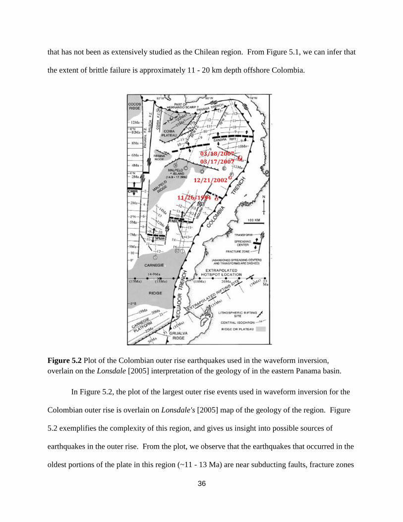
Figure 5.2 Plot of the Colombian outer rise earthquakes used in the waveform inversion,

overlain on the Lonsdale [2005] interpretation of the geology of in the eastern Panama basin.

In Figure 5.2, the plot of the largest outer rise events used in waveform inversion for the

Colombian outer rise is overlain on Lonsdale's [2005] map of the geology of the region. Figure

5.2 exemplifies the complexity of this region, and gives us insight into possible sources of

earthquakes in the outer rise. From the plot, we observe that the earthquakes that occurred in the

oldest portions of the plate in this region (~11 - 13 Ma) are near subducting faults, fracture zones

03/18/2007

03/17/2007

12/21/2002

11/26/1994

37

and rifts. The 03/17/2007 and 03/18/2007 are the northernmost events, and they appear to occur

along a fracture zone oriented perpendicular with respect to the trench, south of the Sandra Rift.

The 12/21/2002 event appears to be possibly influenced by the end of a long abandoned

spreading center or transform oblique to the trench. The 11/26/1994 event occurred in close

proximity to an unknown rift, no longer spreading [Lonsdale, 2005] north of the Yaquina graben.

These observations lead us to infer that these outer rise events are not due to the reactivation of

pre-existing faults due to subducting features in this region. These new faults must have been a

result of the bending forces as the Nazca plate subducts since the focal mechanism orientations

do not match the perpendicularly subducting pre-existing faults. Although the pre-existing faults

could have weakened the plate already, and the earthquakes in this study may be the further

rupture of the faults created by lithospheric bending stresses.

38

CHAPTER 6: CONCLUSIONS AND FUTURE WORK

Both the Colombia and Chile outer rise undergo far more extensional faulting than

compressional faulting. There were no compressional events within the time frame of the data

used in this study, which makes it difficult to constrain the neutral plane. The most recent

compressional events in the Chile outer rise were the events of 1981 and 1982 at 30 and 27 km

depth, respectively [Clouard et al., 2007]. These depths of compressional events seem to

correspond with our inference that the extent of brittle failure is at ~25 km depth for the Chile

region. For Colombia, we infer that the extent of brittle faulting is ~15-20 km depth. We infer

that these depths are possibly the extent to which water can penetrate into the lithosphere.

Whether or not subducting features impact the nucleation of outer rise earthquakes is still not

constrained but unlikely, since the gaps in outer rise event clusters along the Nazca plate still

have subducting structures such as the Peru basin, Easter Fault zone and Nazca Ridge, and Chile

basin within the vicinity of 12 S, 18 S, and 20 S – 30 S.

In future studies, we would like to incorporate the loading history of the plate to calculate

the yield stress envelopes for the oceanic lithosphere in the outer rise. If tomographic data were

available in the study areas, comparing our results with that of the extent of brittle failure to the

depth of water logged faults would help constrain the depth of hydration and brittle failure.

Additionally, we could investigate our method further by incorporating smaller magnitude outer

rise earthquakes and the earthquakes occurring landward of the trench but still within the

subducting Nazca plate. By expanding our methods thusly, we could further constrain the state

of stress within the Nazca plate.

39

APPENDIX

Waveform Inversion results and Depth Estimation plots for all earthquakes.

All plots follow the following descriptions:

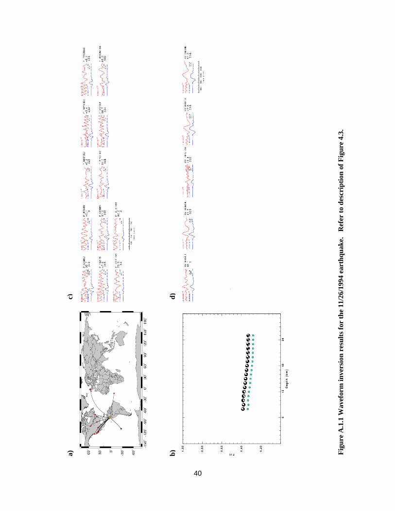
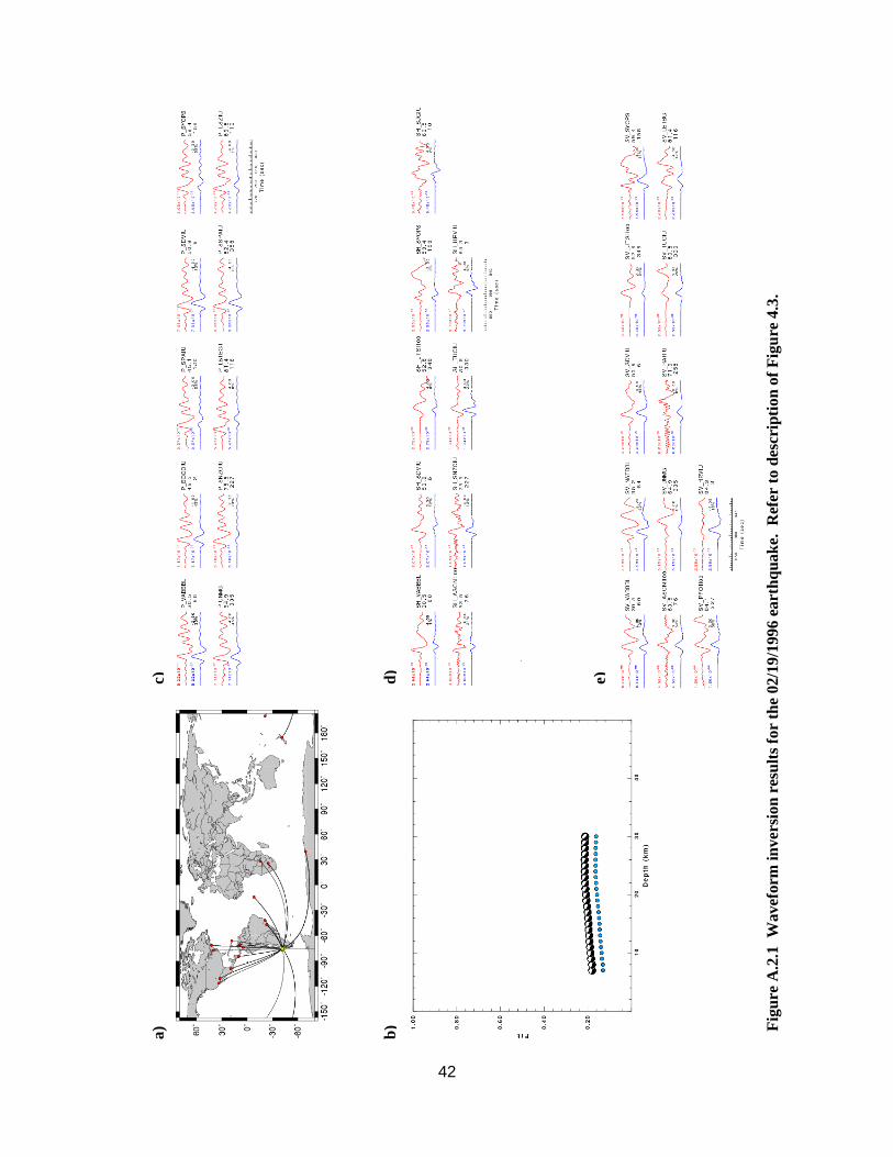
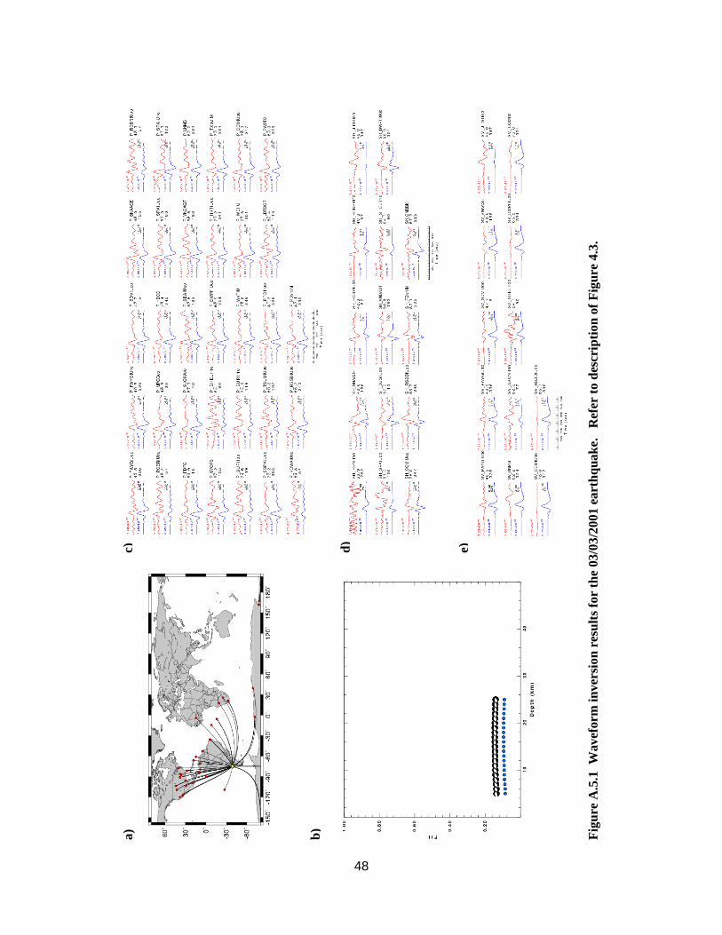
Waveform Inversion Plots: (a) Depicts a map of all stations used in the inversion with the yellow star as

the epicenter and red dots as stations. (b) Shows best fit as a function of depth with the best fit moment

tensor and depth, strike, dip, slip, magnitude, and fit also displayed. P-, SH-, and SV- waves are shown in

c, d, and e respectively. The upper black number to the right of each predicted trace is the time shift

required for maximum correlation between the observed and predicted traces. The lower black number

gives the percentage of variance reduction to characterize the individual goodness of fit.

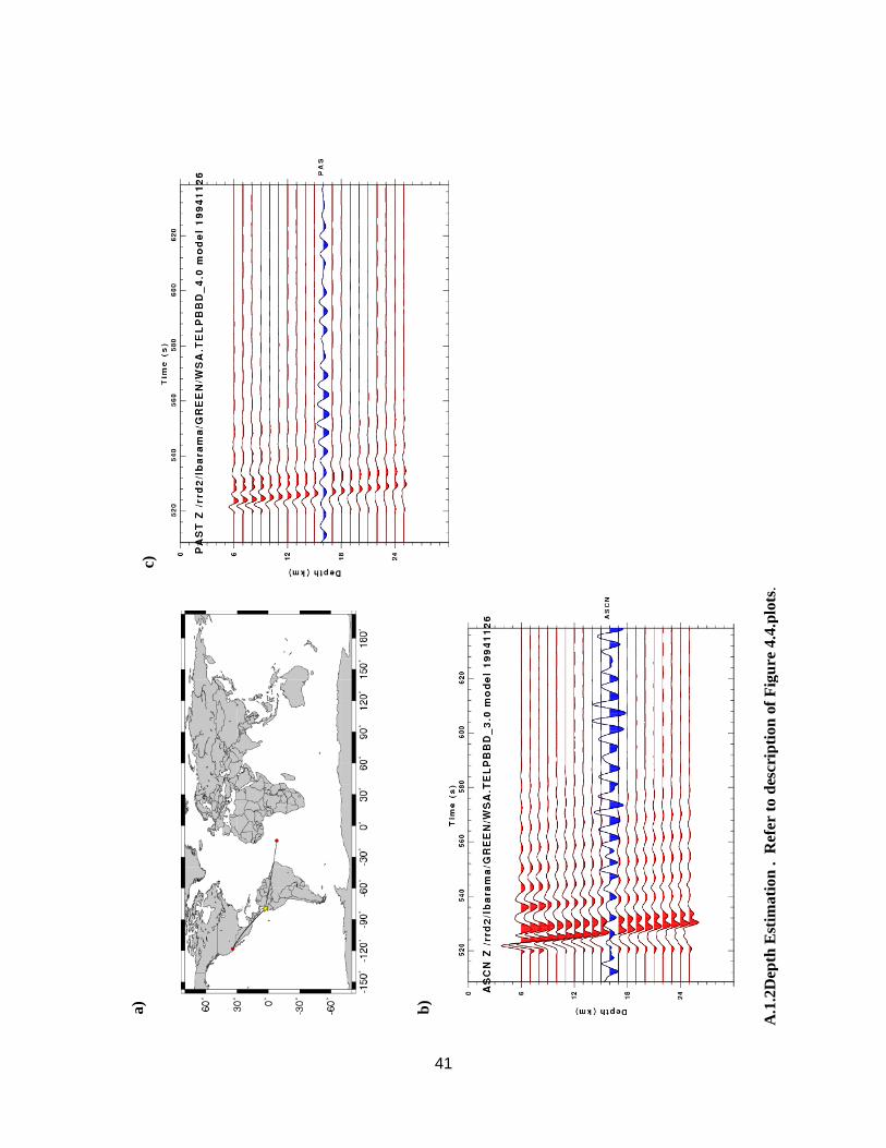
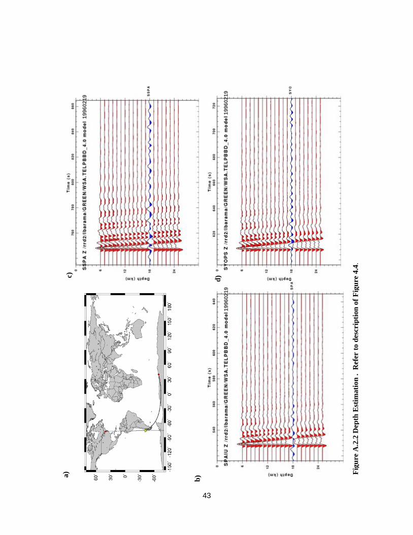
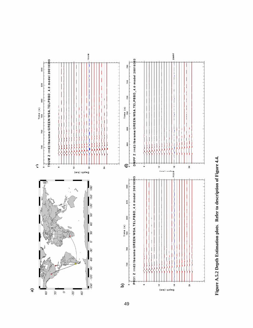
Depth Estimation Plots: (a) shows the global map of stations used for the depth estimation. The yellow

star is the epicenter and the red dots are the stations. Figures b and onward depict the observed

seismogram in blue for the specific station and the synthetics in red. The x-axis shows time in seconds

and the y-axis is depth in kilometers.

40

Fig

ure

A.1

.1 W

avef

orm

in

ver

sio

n r

esu

lts

for

the

11/2

6/1

994 e

art

hq

uak

e.

Ref

er t

o d

escri

pti

on

of

Fig

ure

4.3

.

c)

d)

a)

b)

41

b)

a)

c)

A.1

.2D

epth

Est

ima

tio

n .

R

efer

to

des

cri

pti

on

of

Fig

ure

4.4

.plo

ts.

42

Fig

ure

A.2

.1

Wav

eform

in

ver

sio

n r

esu

lts

for

the

02/1

9/1

996

eart

hq

uak

e.

Ref

er t

o d

escr

ipti

on

of

Fig

ure

4.3

.

c)

d)

a)

b)

e)

43

b) a)

c)

Fig

ure

A.2

.2 D

epth

Est

ima

tio

n .

Ref

er t

o d

escr

ipti

on

of

Fig

ure

4.4

.

d)

19960219

19960219

19960219

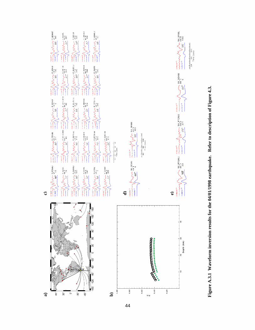
44

Fig

ure

A.3

.1

Wav

eform

in

ver

sio

n r

esu

lts

for

the

04/0

1/1

998

eart

hq

uak

e.

Ref

er t

o d

escri

pti

on

of

Fig

ure

4.3

.

c)

d)

a)

b)

e)

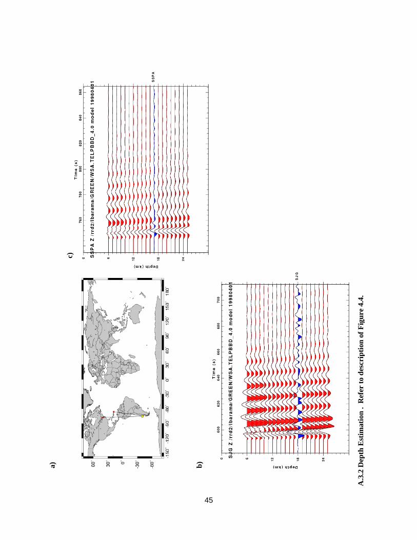
45

b)

a)

c)

A.3

.2 D

epth

Est

imati

on

. R

efer

to

des

cri

pti

on

of

Fig

ure

4.4

.

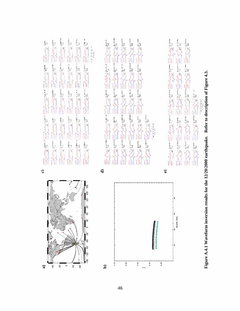
46

Fig

ure

A.4

.1 W

avef

orm

in

ver

sion

res

ult

s fo

r th

e 12/2

0/2

000 e

art

hq

uak

e.

Ref

er t

o d

escri

pti

on

of

Fig

ure

4.3

.

c)

d)

a)

b)

e)

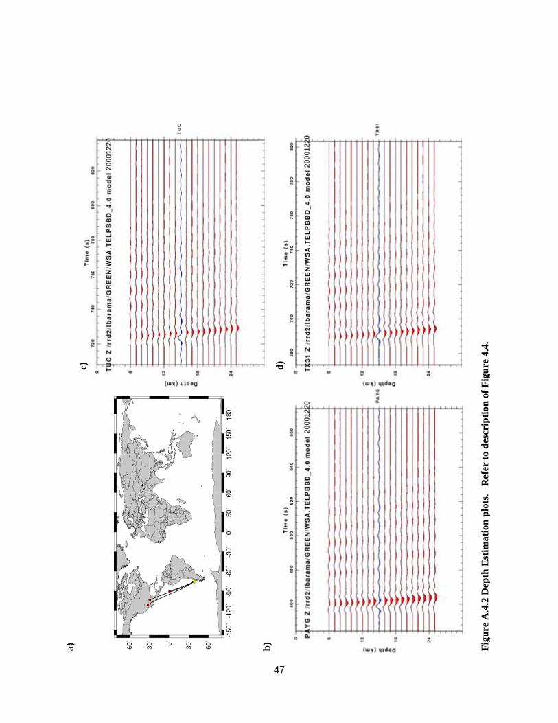
47

b)

a)

c)

Fig

ure

A.4

.2 D

epth

Est

ima

tio

n p

lots

.

Ref

er t

o d

escr

ipti

on

of

Fig

ure

4.4

.

d)

20001220

20001220

20001220

48

Fig

ure

A.5

.1

Wav

eform

in

ver

sio

n r

esu

lts

for

the

03/0

3/2

001

eart

hq

uak

e.

Ref

er t

o d

escri

pti

on

of

Fig

ure

4.3

.

c)

d)

a)

b)

e)

49

a)

c)

Fig

ure

A.5

.2 D

epth

Est

ima

tio

n p

lots

. R

efer

to d

escr

ipti

on

of

Fig

ure

4.4

.

d)

b)

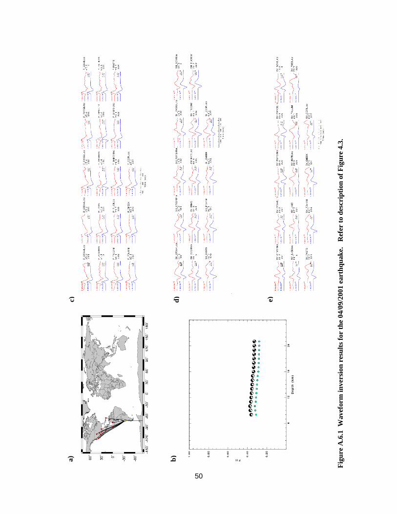
50

Fig

ure

A.6

.1

Wav

eform

in

ver

sio

n r

esu

lts

for

the

04/0

9/2

001 e

art

hq

uak

e.

Ref

er t

o d

escri

pti

on

of

Fig

ure

4.3

.

c)

d)

a)

b)

e)

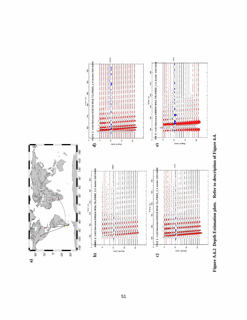
51

a)

c)

Fig

ure

A.6

.2

Dep

th E

stim

ati

on

plo

ts.

Ref

er t

o d

escri

pti

on

of

Fig

ure

4.4

.

d)

b)

e)

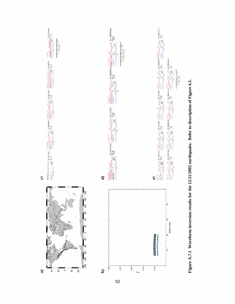
52

Fig

ure

A.7

.1

Wav

eform

in

ver

sio

n r

esu

lts

for

the

12/2

1/2

002 e

art

hq

uak

e.

Ref

er t

o d

escr

ipti

on

of

Fig

ure

4.3

.

c)

d)

a)

b)

e)

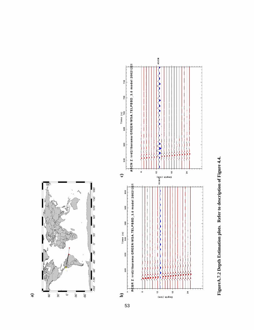
53

a)

c)

Fig

ure

A.7

.2 D

epth

Est

ima

tio

n p

lots

. R

efer

to d

escr

ipti

on

of

Fig

ure

4.4

.

b)

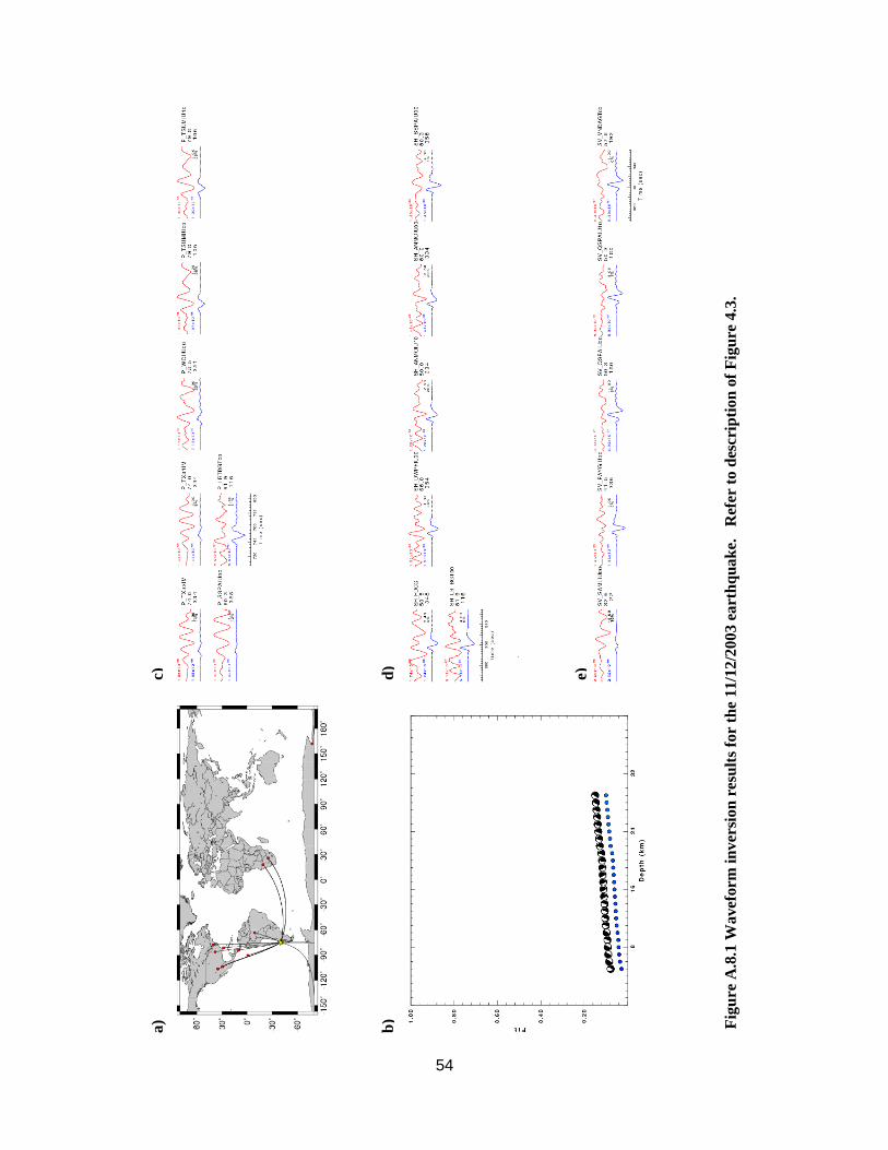
54

Fig

ure

A.8

.1 W

avef

orm

in

ver

sio

n r

esu

lts

for

the

11/1

2/2

003

eart

hq

uak

e. R

efer

to d

escri

pti

on

of

Fig

ure

4.3

.

c)

d)

a)

b)

e)

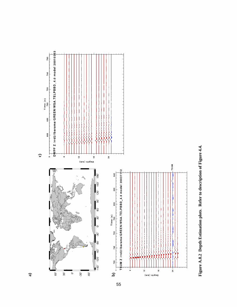
55

b)

a)

c)

Fig

ure

A.8

.2

Dep

th E

stim

ati

on

plo

ts. R

efer

to d

escri

pti

on

of

Fig

ure

4.4

.

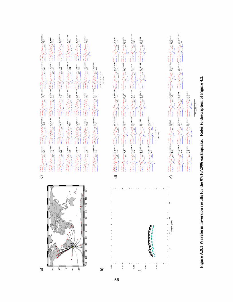
56

Fig

ure

A.9

.1 W

avef

orm

in

ver

sio

n r

esu

lts

for

the

07/1

6/2

006

eart

hq

uak

e.

Ref

er t

o d

escri

pti

on

of

Fig

ure

4.3

.

c)

d)

a)

b)

e)

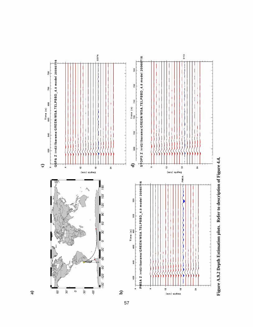
57

b)

a)

c)

Fig

ure

A.9

.2 D

epth

Est

ima

tio

n p

lots

. R

efer

to d

escr

ipti

on

of

Fig

ure

4.4

.

d)

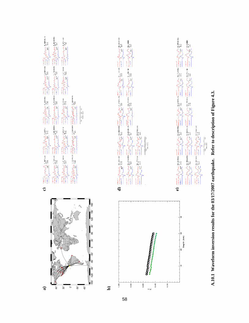
58

A.1

0.1

W

avef

orm

in

ver

sio

n r

esu

lts

for

the

03

/17/2

007

eart

hq

uak

e. R

efer

to d

escri

pti

on

of

Fig

ure

4.3

.

c)

d)

a)

b)

e)

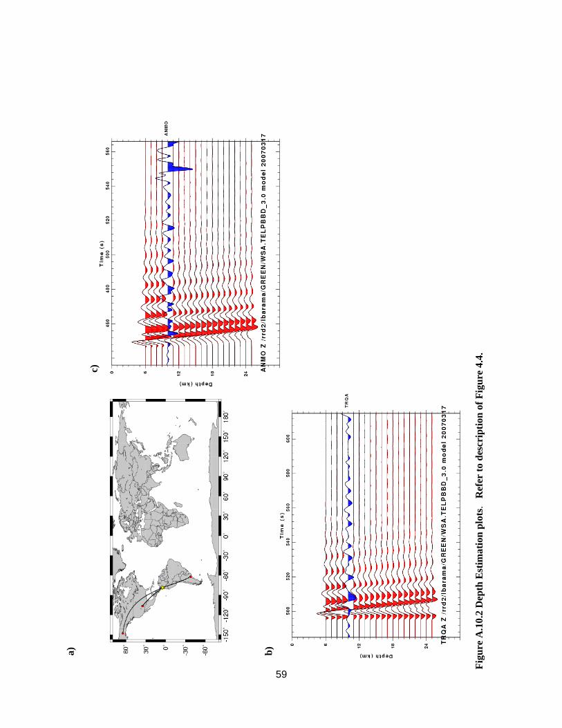
59

b)

a)

c)

Fig

ure

A.1

0.2

Dep

th E

stim

ati

on

plo

ts.

R

efer

to d

escri

pti

on

of

Fig

ure

4.4

.

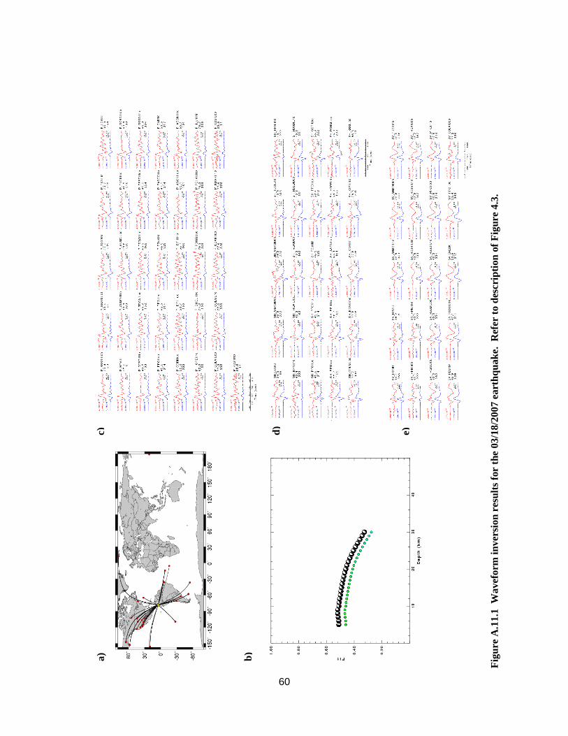
60

Fig

ure

A.1

1.1

W

av

efo

rm i

nv

ersi

on

res

ult

s fo

r th

e 03/1

8/2

007

eart

hq

uak

e.

Ref

er t

o d

escri

pti

on

of

Fig

ure

4.3

.

c)

d)

a)

b)

e)

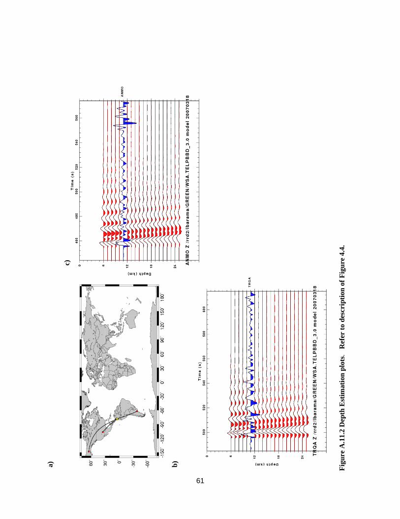
61

b)

a)

c)

Fig

ure

A.1

1.2

Dep

th E

stim

ati

on

plo

ts.

Ref

er t

o d

escri

pti

on

of

Fig

ure

4.4

.

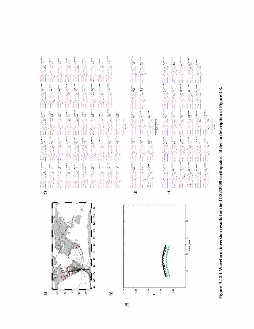
62

Fig

ure

A.1

2.1

Wav

efo

rm i

nv

ersi

on

res

ult

s fo

r th

e 11/2

2/2

009

eart

hq

uak

e.

Ref

er t

o d

escri

pti

on

of

Fig

ure

4.3

.

c)

d)

a)

b)

e)

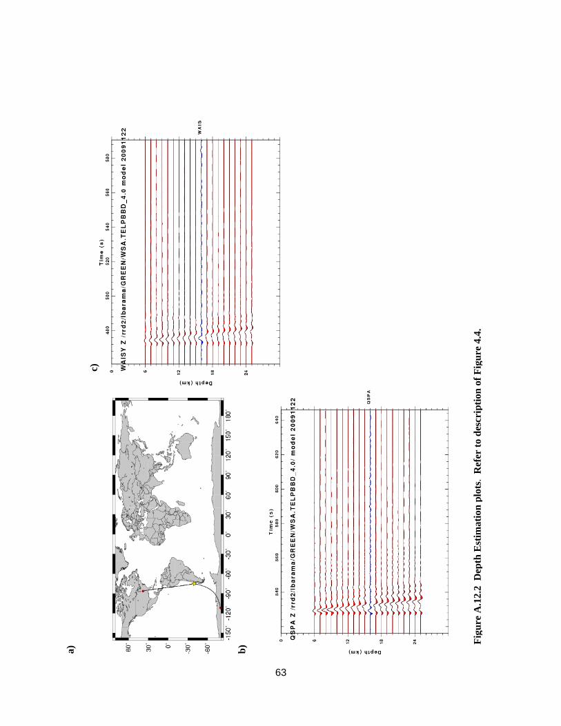
63

b)

a)

c)

Fig

ure

A.1

2.2

D

epth

Est

ima

tio

n p

lots

. R

efer

to d

escri

pti

on

of

Fig

ure

4.4

.

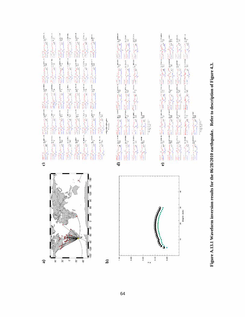
64

Fig

ure

A.1

3.1

Wav

efo

rm i

nv

ersi

on

res

ult

s fo

r th

e 06/2

8/2

010

eart

hq

uak

e.

Ref

er t

o d

escri

pti

on

of

Fig

ure

4.3

.

c)

d)

a)

b)

e)

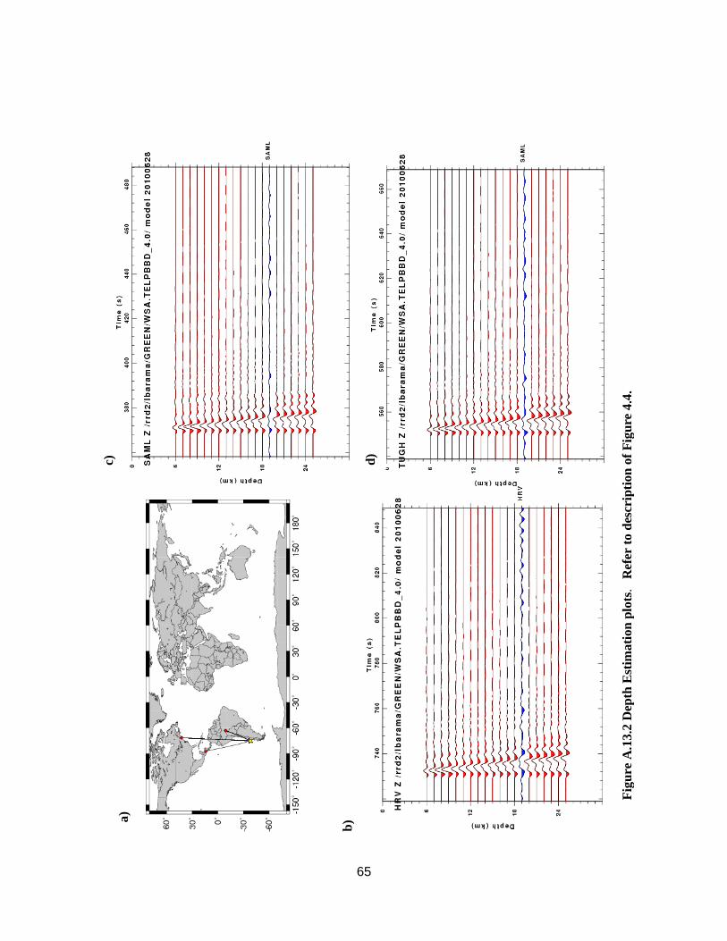
65

b) a

)

c)

Fig

ure

A.1

3.2

Dep

th E

stim

ati

on

plo

ts. R

efer

to d

escri

pti

on

of

Fig

ure

4.4

.

d)

66

BIBLIOGRAPHY

Barcheck C.G., D.A. Wiens, P.E. van Keken, and B.R. Hacker (2012), The relationship of

intermediate-and deep-focus seismicity to the hydration and dehydration of subducting

slabs, Earth Planet. Sci. Lett., 153-160.

Brace, W.F., and D.L. Kohlstedt (1980), Limits on lithospheric stress imposed by laboratory

experiments, J. Geophys. Res., 85, 6248-6252.

Caldwell, J.G., W.F. Haxby, D.E. Karig, and D.L. Turcotte (1976), On the applicability of a

universal elastic trench profile, Earth Planet. Sci. Lett., 31, 239-246.

Chapple, W.M., and D.W. Forsyth (1979), Earthquakes and bending of plates at trenches, J.

Geophys. Res., 84(B12), 6729-6749.

Christensen, D.H., and L.J. Ruff (1988), Seismic coupling and outer rise earthquakes,

Geophys. Res.,93(B11),13,421-31,444, doi: 10.1029/JB093iB11p13421.

Clouard, V., J. Campos, A. Lemoine, A. Pérez, and E. Kausel (2007), Outer rise stress changes

related to the subduction of the Juan Fernández Ridge, central Chile. J. Geophys. Res.,

112, doi:10.1029/2005JB003999.

Contreras-Reyes, E., I. Grevemeyer, E.R. Fluej, and M. Scherwath (2007), Alteration of the

subducting oceanic lithospere at the southern central Chile trench-outer rise, Geochem.

Geophys. Geosyst., 8(7), Q07003, doi:10.1029/2007GC001632.

Craig, T.J., A. Copley and J. Jackson (2014), A reassessment of outer-rise seismicity and its

implications for the mechanics of oceanic lithosphere, Geophys. J. Int. 197, 63–89.

Ekström, G., M. Nettles, and A. M. Dziewonski (2012), The global CMT project 2004-2010:

Centroid-moment tensors for 13,017 earthquakes, Phys. Earth Planet. Int., 200-201, 1-9,

doi:10.1016/j.pepi.2012.04.002.

Emry, E.L., D.A. Wiens, H. Shiobara, and H. Sugioka (2011), Seismogenic characteristics of the

Northern Mariana shallow thrust zone from local array data, Geochem. Geophys.

Geosyst., 12(12), Q12008, doi: 10.10292011GC003853.

Emry, E.L., D.A. Wiens, and D. Garcia-Castellanos (2014), Faulting within the Pacific plate at

the Mariana Trench: Implications for plate interface coupling and subduction of hydrous

minerals, J. Geophys. Res. Solid Earth, 119, doi:10.1002/2013JB010718.

67

Fromm, R., P. Alvarado, S. L. Beck, and G. Zandt (2006), The April 9, 2001 Juan Fernández

Ridge (M w 6.7) Tensional Outer-Rise Earthquake and its Aftershock Sequence,

J. Seis., 10(2), 163-170.

Garcia-Castellanos, D., M. Torne, and M. Fernàndez (2000), Slab pull effects from a flexural

analysis of the Tonga and Kermadec trenches (Pacific Plate), Geophys. J. Int., 141(2),

479–484, doi:10.1046/j.1365-246x.2000.00096.x.

Garcia, P.P., C.A. Vargas, and H. Monsalve (2007), Geometric model of the Nazca plate

subduction in Southwest Colombia, Earth Sci. Res. J.,11( 2), 117-130.

Gill, J. B. (1981), Orogenic Andesites and Plate Tectonics, pp. 390, Springer, New York.

Goetze, C., and B. Evans (1979), Stress and temperature in the bending lithosphere as

constrained by experimental rock mechanics, Geophys. J. R. Astron. Soc., 59(3),

doi:10.1111/j.1365-246X.1979.tb02567.x

Grevemeyer, I., N. Kaul, J.L. Diaz-Naveas, H. Villinger, C.R. Ranero, and C. Reichert (2005),

Heat flow and bending-related faulting at subduction trenches: case studies offshore of

Nicaragua and Central Chile, Earth planet. Sci. Lett., 236, 238–248.

Grevemeyer, I., C.R. Ranero, , E.R. Flueh, , D. Klaeschen, and J. Bialas (2007), Passive and

active seismological study of bending-related faulting and mantle serpentinization at the

Middle America trench, Earth planet. Sci. Lett., 258, 528–542.

Gutscher, M.A., W. Spakman, H. Bijwaard and E. R. Engdahl (2000), Geodynamics of flat

subduction: Seismicity and tomographic constraints from the Andean margin, Tectonics,

19(5), 814-833.

Gutscher, M.A. (2002), Andean subduction styles and their effect on thermal structure and

interplate coupling, J. S. Amer. Earth Sci., 15(2002), 3-10, PII:S0895-9811(02)00002-0.

Herrmann, R. B. (1976), Focal depth determination from the signal character of long-period P-

waves, Bull. Seism. Soc. Am. 66, 1221-1232.

Herrmann, R. B. (2013), Computer programs in seismology: An evolving tool for instruction and

research, Seis. Res. Lett. 84, 1081-1088, doi:10.1785/0220110096.

Hirschmann, M.M. (2006), Water, melting, and the deep Earth H2O cycle, Annu. Rev. Earth

Planet. Sci., 34, 629–653, doi:10.1146/annurev.earth.34.031405.125211.

68

Hudson, J.A. (1969), A quantitative evaluation of seismic signals at teleseismic distances, II.

Body waves and surface waves from an extended source, Geophys. J.,18, 353-370.

Jordan, T.H., and K.A. Sverdrup (1981), Teleseismic location techniques and their

application to earthquake clusters in the South-Central Pacific, Bull. Seis. Soc. Am.,

71(4), 1105-1130.

Kanamori, H (1971), Seismological evidence for lithospheric normal faulting: the Sanriku

earthquake of 1933, Phys. Earth planet. Int., 4, 289-300.

Kirby, S. H. (1980), Tectonic stresses in the lithosphere: Constraints provided by the

experimental deformation of rocks, J. Geophys. Res., 85, 6353-6363.

Korenaga, J. (2007), Thermal cracking and the deep hydration of oceanic lithosphere: A key to

the generation of plate tectonics?, J.Geophys.Res.,112,B05408,

doi:10.1029/2006JB004502.

Lay, T., L. Astiz, H. Kanamori, and D.H. Christensen (1989), Temporal variation of large

intraplate earthquakes in coupled subduction zones, Phys. Earth Planet. Int., 54(3-

4), 258-312.

Lefeldt, M., I. Grevemeyer, J. Goßler, and J. Bialas (2009), Intraplate seismicity and related

mantle hydration at the Nicaraguan trench outer rise, Geophys. J. Int.,178(2), 742-752,

doi: 10.1111/j.1365-246X.2009.04167.x.

Lefeldt, M., and I. Grevemeyer (2008), Centroid depth and mechanism of trench-outer rise

earthquakes, Geophys. J. Int., 172, 240-251, doi: 10.1111/j.1365-246X.2007.03616.x.

Lomax, A., J. Virieux, P. Volant, and C. Berge (2000), Probabilistic earthquake location in 3D

and layered models: introduction of a Metropolis–Gibbs method and comparison with

linear locations, in Advances in Seismic Event Location, pp. 101–134, eds. Thurber, C.H.

& Rabinowitz, N., Kluwer, Amsterdam.

Lonsdale, P. (2005), Creation of the Cocos and Nazca plates by fission of the Farallon plate,

Tectonophysics, 404, 237-264.

McGinnis, S. (2001), On the effects of geometry in discrete element numerical earthquake

simulations, PhD thesis, University of Colorado.

69

McKenzie, D., J. Jackson and K. Priestley (2005), Thermal structure of oceanic and continental

lithosphere, Earth planet. Sci. Lett., 233, 337–349.

Moscoso, E., and E. Contreras-Reyes (2012), Outer rise seismicity related to the Maule, Chile

2010 megathrust earthquake and hydration of the incoming oceanic lithosphere, Geology,

39(3), 564-572, doi:10.5027/andgeoV39n3-a12.

O’Neill, C., A. M. Jellinek, and A. Lenardic (2007), Conditions for the onset of plate tectonics

on terrestrial planets and moons, Earth Planet. Sci. Lett., 261, 20–32,

doi:10.1016/j.epsl.2007.05.038.

Peacock, S.M. (2001), Are the lower planes of double seismic zones caused by serpentine

dehydration in subducting oceanic mantle, Geology, 29(4), 299-302, doi: 10.1130/0091-

7613(2001)029<0299:ATLPOD>2.0.CO;2.

Ranero, C. R., J. Phipps Morgan, K. McIntosh, and C. Reichert (2003), Bending related faulting

and mantle Serpentinization at the Middle America trench, Nature, 425 (6956), 367-373,

doi: 10.1038/nature01961.

Ranero, C. R., and V. Sallares (2004), Geophysical evidence for hydration of the crust and

mantle of the Nazca plate during bending at the north Chile trench, Geology, 32(7), 549-

552, doi: 10.1130/G20379.1.

Rüpke, L. H., J. Phipps Morgan, M. Hort, and J.A.D. Connolly (2004), Serpentine and the

subduction zone water cycle, Earth Planet. Sci. Lett., 223(1–2), 17–34,

doi:10.1016/j.epsl.2004.04.018.

Seno, T., and Y. Yamanaka (1996), Double seismic zones, compressional deep trench-outer rise

events and superplumes in Subduction Top to Bottom (G.E. Bebout, D.W. Scholl, S.H.

Kirby, J.P. Platt, editors), Geophysical Monograph, 96: 347-355.

Shearer, P.M. (2009), Introduction to Seismology, Second Edition, Cambridge University Press,

Cambridge.

Stein, S., and D.A. Weins (1986), Depth Determination fo shallow teleseismic earthquakes:

methods and results, J. Geophys. Res., 24(4), 806-832 doi: 10.1029/RG024i004p00806.

Supak, S., D.R. Bohnenstiehl, and W.R. Buck (2006), Flexing is not stretching: An analogue

study of flexure-induced fault populations, Earth Planet. Sci. Lett. 246, 125–137.

70

Van Avendonk, H.J.A., W.S. Holbrook, D. Lizarralde, and P. Denyer (2011), Structure and

serpentinization of the subducting Cocos plate offshore Nicaragua and Costa Rica,

Geochem. Geophys. Geosyst., 12, Q06009, doi:10.1029/2011GC003592.

Van Keken, P.E., B.R. Hacker, E.M. Syracuse, and G.A. Abers (2011), Subduction Factory: 4.

Depth-dependent flux of H2O from subducting slabs worldwide, J. Geophys. Res., 116,

B01401, doi: 10.1029/2010JB007922.

Wada, I., M.D. Behn, and A.M. Shaw (2012), Effects of heterogeneous hydration in the

incoming plate, slab rehydration, and mantle wedge hydration on slab-derived H2O flux

in subduction zones, Earth Planet. Sci. Lett., 353, 60-71.

Wolfe, C.J., S.C. Solomon, P.G. Silver, J.C. VanDecar, and R.M. Russo (2002), Inversion of

body-wave delay times for mantle structure beneath the Hawaiian islands: results from

the PELENET experiment, Earth Planet. Sci. Lett., 198(1–2), 129-145.

71

VITA AUCTORIS

Louisa Barama was born in 1990 in Denmark. She graduated from Brookwood High

School in 2008 and received her Bachelor of Science in Physics from Oglethorpe University in

2012. In the Fall of 2012, Louisa began the pursuit of a Master of Science in Geophysics at

Saint Louis University.

Documents

OUTER RISE SEISMICITY OF THE SUBDUCTING … RISE SEISMICITY OF THE SUBDUCTING NAZCA PLATE: PLATE STRESS DISTRIBUTION, FAULT ORIENTATION AND PLATE HYDRATION Louisa Barama, B.S. An Abstract