Outer Billiards on Kites

by

Richard Evan Schwartz

1

PrefaceOuter billiards is a basic dynamical system defined relative to a convex shapein the plane. B.H. Neumann introduced outer billiards in the 1950s, and J.Moser popularized outer billiards in the 1970s as a toy model for celestialmechanics. Outer billiards is an appealing dynamical system because of itssimplicity and also because of its connection to such topics as interval ex-change maps, piecewise isometric actions, and area-preserving actions. Thereis a lot left to learn about these kinds of dynamical systems, and a good un-derstanding of outer billiards might shed light on the more general situation.

The Moser-Neumann question, one of the central problems in this subject,asks Does there exist an outer billiards system with an unbounded orbit? Untilrecently, all the work on this subject has been devoted to proving that all theorbits are bounded for various classes of shapes. We will detail these resultsin the introduction.

Recently we answered the Moser-Neumann question in the affirmative byshowing that outer billiards has an unbounded orbit when defined relative tothe Penrose kite, the convex quadrilateral that arises in the famous Penrosetiling. Our proof involves special properties of the Penrose kite, and naturallyraises questions about generalizations.

In this monograph we will give a more general and robust answer to theMoser-Neumann question. We will prove that outer billiards has unboundedorbits when defined relative to any irrational kite. A kite is probably bestdefined as a “kite-shaped” quadrilateral. (See the top of §1.2 for a non-circular definition.) The kite is irrational if it is not affinely equivalent toa quadrilateral with rational vertices. Our proof uncovers some of the deepstructure underlying outer billiards on kites, and relates the subject to suchtopics as self-similar tilings, polytope exchange maps, and the modular group.

I discovered every result in this monograph by experimenting with mycomputer program, Billiard King, a Java-based graphical user interface. Forthe most part, the material here is logically independent from Billiard King,but I encourage the serious reader of this monograph to download BilliardKing from my website 1 and play with it. My website also has an interactiveguide to this monograph, in which many of the basic ideas and constructionsare illustrated with interactive Java applets.

1www.math.brown.edu/∼res

2

There are a number of people I would like to thank. I especially thankSergei Tabachnikov, whose great book Geometry and Billiards first taughtme about outer billiards. Sergei has constantly encouraged me as I haveinvestigated this topic, and he has provided much mathematical insight alongthe way.

I thank Yair Minsky for his work on the punctured-torus case of the End-ing Lamination Conjecture. It might seem strange to relate outer billiardsto punctured-torus bundles, but there seems to me to be a common theme.In both cases, one studies the limit of geometric objects indexed by rationalnumbers and controlled in some sense by the Farey triangulation.

I thank Eugene Gutkin for the explanations he has given me about hiswork on outer billiards. The work of Gutkin-Simanyi and others on theboundedness of the orbits for rational polygons provided the theoretical un-derpinnings for some of my initial computer investigations.

I thank Jeff Brock, Peter Doyle, David Dumas, Richard Kent, Howie Ma-sur, Curt McMullen, John Smillie, and Ben Wieland, for their mathematicalinsights and general interest in this project.

I thank the National Science Foundation for their continued support,currently in the form of the grant DMS-0604426.

I dedicate this monograph to my parents, Karen and Uri.

3

Table of Contents1. Introduction 6

Part I 162. The Arithmetic Graph 173. The Hexagrid Theorem 234. Odd Approximation and Period Copying 325. Existence of Erratic Orbits 376. The Orbit Dichotomy 437. The Density of Periodic Orbits 478. Symmetries of the Arithmetic Graph 529. Further Results and Conjectures 58

Part II 6710. The Master Picture Theorem 6811. The Pinwheel Lemma 7712. The Torus Lemma 9013. The Strip Functions 9914. Proof of the Master Picture Theorem 10615. Some Formulas 111

Part III 11816. Proof of the Embedding Theorem 11917. Extension and Symmetry 12618. The Structure of the Doors 13019. Proof of the Hexagrid Theorem I 13520. Proof of the Hexagrid Theorem II 142

Part IV 15521. The Copy Theorem 15622. Existence of Superior Sequences 16823. Proof of the Decomposition Theorem 17824. Proof of Theorem 4.2 184

25. References 187

4

1 Introduction

1.1 History of the Problem

B.H. Neumann [N] introduced outer billiards in the late 1950s. In the 1970s,J. Moser [M1] popularized outer billiards as a toy model for celestial me-chanics. One appealing feature of polygonal outer billiards is that it givesrise to a piecewise isometric mapping of the plane. Such maps have close con-nections to interval exchange transformations and more generally to polygonexchange maps. See [T1] and [DT] for an exposition of outer billiards andmany references.

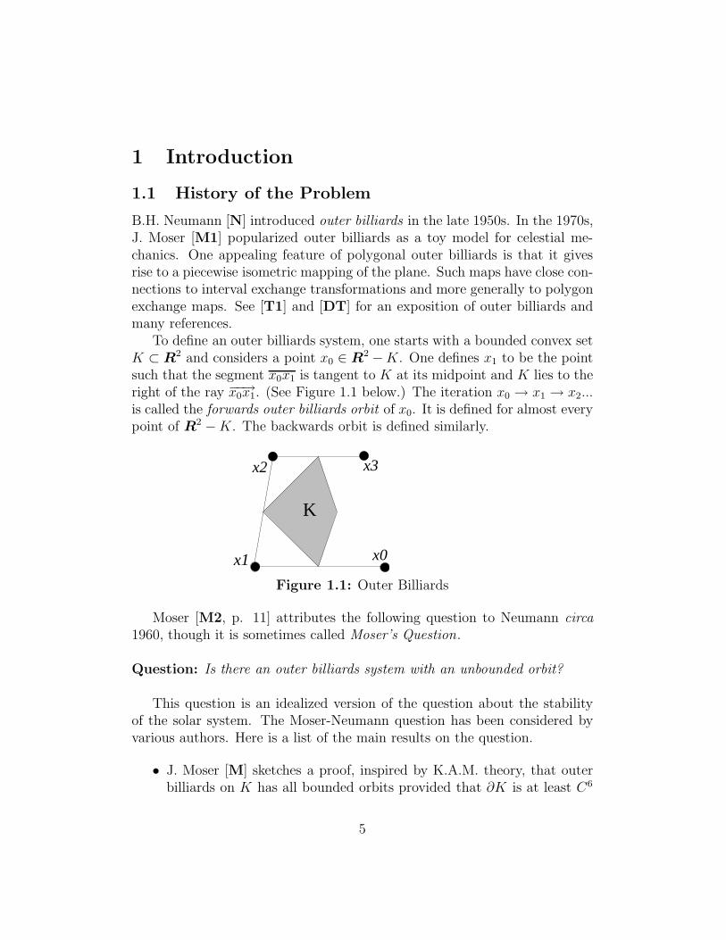
To define an outer billiards system, one starts with a bounded convex setK ⊂ R2 and considers a point x0 ∈ R2 −K. One defines x1 to be the pointsuch that the segment x0x1 is tangent to K at its midpoint and K lies to theright of the ray −−→x0x1. (See Figure 1.1 below.) The iteration x0 → x1 → x2...is called the forwards outer billiards orbit of x0. It is defined for almost everypoint of R2 −K. The backwards orbit is defined similarly.

x2

x1 x0

x3

K

Figure 1.1: Outer Billiards

Moser [M2, p. 11] attributes the following question to Neumann circa1960, though it is sometimes called Moser’s Question.

Question: Is there an outer billiards system with an unbounded orbit?

This question is an idealized version of the question about the stabilityof the solar system. The Moser-Neumann question has been considered byvarious authors. Here is a list of the main results on the question.

• J. Moser [M] sketches a proof, inspired by K.A.M. theory, that outerbilliards on K has all bounded orbits provided that ∂K is at least C6

5

smooth and positively curved. R. Douady gives a complete proof in histhesis, [D].

• P. Boyland [B] gives examples of C1 smooth convex domains for whichan orbit can contain the domain boundary in its ω-limit set.

• In [VS], [Ko], and (later, but with different methods) [GS], it is provedthat outer billiards on a quasirational polygon has all orbits bounded.This class of polygons includes rational polygons and also regular poly-gons. In the rational case, all defined orbits are periodic.

• S. Tabachnikov analyzes the outer billiards system for the regular pen-tagon and shows that there are some non-periodic (but bounded) orbits.See [T1, p 158] and the references there.

• D. Genin [G] shows that all orbits are bounded for the outer billiardssystems associated to trapezoids. He also makes a brief numerical studyof a particular irrational kite based on the square root of 2, observespossibly unbounded orbits, and indeed conjectures that this is the case.

• Recently, in [S] we proved that outer billiards on the Penrose kite hasunbounded orbits, thereby answering the Moser-Neumann question inthe affirmative. The Penrose kite is the convex quadrilateral that arisesin the Penrose tiling. See §1.6 for a discussion.

• Very recently, D. Dolgopyat and B. Fayad [DF] show that outer bil-liards around a semicircle has some unbounded orbits. Their proof alsoworks for “circular caps” sufficiently close to the semicircle. This is asecond affirmative answer to the Moser-Neumann question.

The result in [S] naturally raises questions about generalizations. Thepurpose of this monograph is to develop the theory of outer billiards on kitesand show that the phenomenon of unbounded orbits for polygonal outerbilliards is (at least for kites) quite robust. We think that the theory wedevelop here will work for polygonal outer billiards in general, though rightnow a general theory is beyond us.

We mention again that we discovered all the results in the monographthrough computer experimentation. The interested reader can download myprogram, Billiard King, from my website 2.

2www.math.brown.edu/∼res

6

1.2 Main Results

For us, a kite is a quadrilateral of the form K(A), with vertices

(−1, 0); (0, 1) (0,−1) (A, 0); A ∈ (0, 1). (1)

Figure 1.1 shows an example. We call K(A) (ir)rational iff A is (ir)rational.Outer billiards is an affinely invariant system, and any quadrilateral that istraditionally called a kite is affinely equivalent to some K(A).

Let Zodd denote the set of odd integers. Reflection in each vertex ofK(A)preserves R×Zodd. Hence, outer billiards on K(A) preserves R×Zodd. Wesay that a special orbit on K(A) is an orbit contained in R×Zodd. We calla point in R×Zodd special erratic (relative to the kite) if both the forwardsand backwards orbits of this point are unbounded, and return infinitely oftento every neighborhood of the vertex set of the kite. Define the special erraticset to be the set of special erratic points.

Theorem 1.1 (Erratic Orbit) Relative to any irrational kite, the specialerratic set contains a near-Cantor set.

We say that a near-Cantor set is a set of the form C − C ′, where C is aCantor set, and C ′ is a countable set. The Erratic Orbit Theorem says, inparticular, that outer billiards on any irrational kite has uncountably manyunbounded orbits.

Theorem 1.2 Relative to any irrational kite, any special orbit is periodic orelse unbounded in both directions.

Theorem 1.3 Relative to any irrational kite, the set of periodic special orbitsis open dense in R×Zodd.

The rational cases of Theorems 1.2 and 1.3 follow from the work of [VS],[K], and [GS], In this case, all orbits are periodic. In the irrational case,Theorem 1.1 makes Theorems 1.2 and 1.3 especially interesting. Computerevidence suggests that versions of Theorems 1.2 and 1.3 hold true for allorbits, and not just special orbits. See §9.4 for a discussion.

The monograph has two other main results as well, namely the HexagridTheorem (§3) and the Master Picture Theorem (§10), but these results arenot easily stated without a buildup of terminology. We will discuss these tworesults later on in the introduction.

7

1.3 Rational Kites

We say that p/q is odd or even according as to whether pq is odd or even.In §6 we will construct, for each irrational A ∈ (0, 1), a canonical sequence{pn/qn} of odd rationals that converges to A. The sequence {pn/qn} is similarto the sequence of continued fraction approximants to A. Our approach tothe main results is to get a good understanding of the special orbits relativeto K(pn/qn) and then to take suitable limits.

We find it convenient to work with the square of the outer billiards maprather than the map itself, and our results implicitly refer to the square map.(This has no effect on the results above.)

Let O2(x) denote the square outer billiards orbit of x. Let

Ξ = R+ × {−1, 1}. (2)

Our Pinwheel Lemma, from §11, shows that O2 ∩ Ξ pretty well controls O2

for any special orbit O2. The intuitive idea is that O2(x) generally circulatesaround the kite, and hence returns to Ξ in a fairly regular fashion. We willstate the results about rational kites in terms of O2 ∩ Ξ.

When ǫ ∈ (0, 2/q), the orbit O2(ǫ, 1) has a combinatorial structure inde-pendent of ǫ. See Lemma 2.2. Thus, O2(1/q, 1) is a natural representativeof an orbit that starts out “right next to” the kite vertex (0, 1). This orbitplays a crucial role in our proof of Theorem 1.1.

Let λ(p/q) = 1 if p/q is odd and λ(p/q) = 2 if p/q is even. Our resultsrefer to outer billiards on K(p/q). We set λ = λ(p/q)

Theorem 1.4 O2(1/q, 1) ∩ Ξ has diameter at least λ · (p+ q)/2.

When the time comes, we will assume that p > 1 in our proof. The casep = 1 is still true, but the proof is more tedious.

We think of Theorem 1.4 as a “rational precursor” of Theorem 1.1. Thenext result shows that Theorem 1.4 is sharp to within a factor of 2.

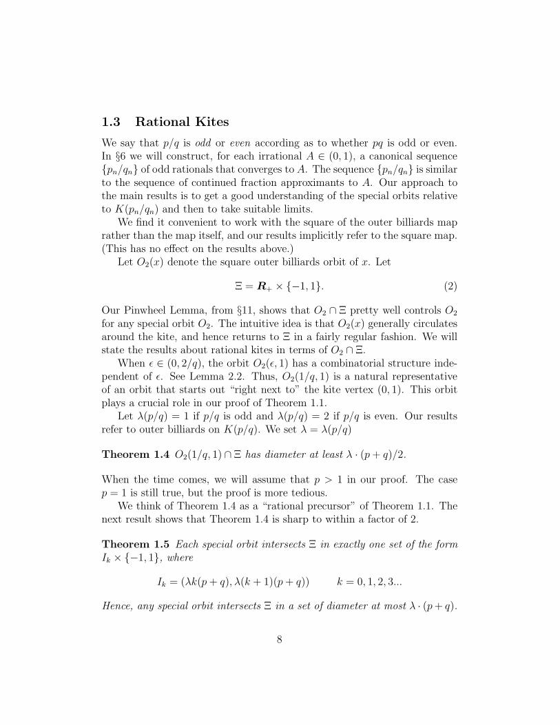
Theorem 1.5 Each special orbit intersects Ξ in exactly one set of the formIk × {−1, 1}, where

Ik = (λk(p+ q), λ(k + 1)(p+ q)) k = 0, 1, 2, 3...

Hence, any special orbit intersects Ξ in a set of diameter at most λ · (p+ q).

8

Theorem 1.5 is similar in spirit to a result in [K]. See §3.5 for a discussion.An outer billiards orbit on K(A) is called stable if there are nearby and

combinatorially identical orbits on K(A′) for all A′ sufficiently close to A.Otherwise, the orbit is called unstable. In the odd case, O2(1/q, 1) is unstable,and this fact is crucial to our proof of Theorem 1.1. It also turns out thatO(3/q, 1) is stable, and this fact is crucial to our proof of Theorem 1.3. Hereis a classification of special orbits.

Theorem 1.6 In the even rational case, all special orbits are stable. In theodd case, the set Ik × {−1, 1} contains exactly two unstable orbits, U+

k andU−

k , and these are conjugate by reflection in the x-axis. In particular, wehave U±

0 = O2(1/q,±1).

1.4 The Arithmetic Graph

All our results about special orbits derive from our analysis of a fundamen-tal object, which we call the arithmetic graph. The principle guiding ourconstruction is that sometimes it is better to understand the abelian groupZ[A] := Z ⊕ZA as a module over Z rather than as a subset of R.

In this section we will explain the idea behind the arithmetic graph. In§2.5 we will give a precise construction.

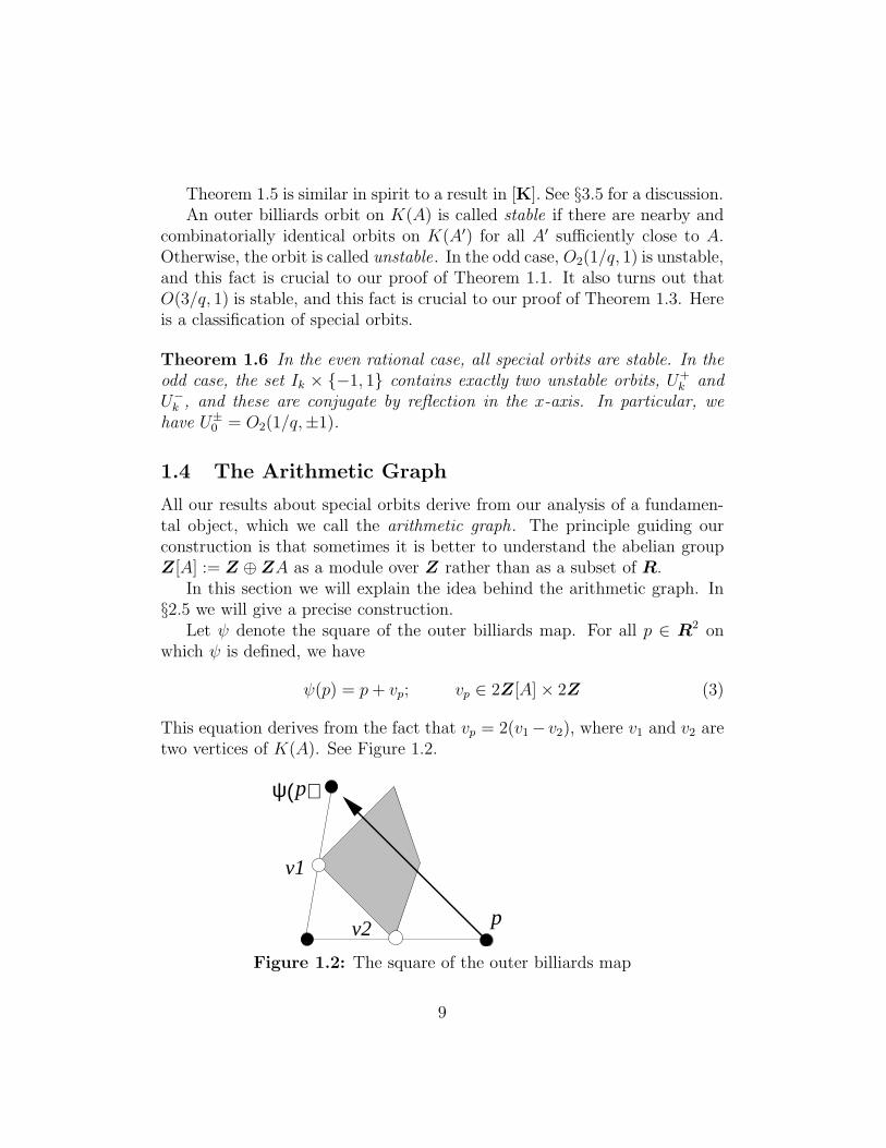
Let ψ denote the square of the outer billiards map. For all p ∈ R2 onwhich ψ is defined, we have

ψ(p) = p+ vp; vp ∈ 2Z[A]× 2Z (3)

This equation derives from the fact that vp = 2(v1− v2), where v1 and v2 aretwo vertices of K(A). See Figure 1.2.

)(ψ

p

p

v1

v2

Figure 1.2: The square of the outer billiards map

9

Let Ξ = R+ × {−1, 1}, as above. The arithmetic graph encodes thearithmetic behavior of the first return map Ψ : Ξ → Ξ. Assuming that theorbit of (2α, 1) is defined, it turns out that

Ψk(2α, 1) = (2α+ 2mkA+ 2nk,±1); mk, nk ∈ Z. (4)

The arithmetic graph Γα(A) is the path in Z2 with vertices (mk, nk), con-nected in the obvious way. We will prove that

(mk+1, nk+1)− (mk, nk) ∈ {−1, 0, 1}2 (5)

Thus Γα(A) is a lattice path that connects nearest neighbors in Z2. In thenext section we show some pictures. The reader can see pictures for anysmallish parameter using either Billiard King or the interactive guide to themonograph.

When A = p/q is rational, we set α = 1/(2q), and simplify our notation toΓ(p/q). In the odd case, Γ(p/q) is an open polygonal curve, invariant undertranslation by (q,−p). In the even case, Γ(p/q) is an embedded polygon.

We will prove Theorem 1.4 by showing that Γ(p/q) rises on the order ofp + q units away from the line of slope −p/q through the origin. This lineis invariant under translation by (q,−p). Theorems 1.5 and 1.6 are basedon a more global version of Γ(p/q), where we consider simultaneously thearithmetic graphs of all orbits of the form

(1/q + 2Z[A])× {−1, 1} (6)

The resulting object, which we call Γ(p/q), turns out to be a disjoint unionof embedded polygons and embedded infinite polygons. This is the contentof our Embedding Theorem. See §2.6. Each component corresponds to acombinatorial equivalence class of special orbit. The component is a polygoniff the orbit is stable.

In §3 we will explain a general structural result for the arithmetic graph,the Hexagrid Theorem. Part III of the monograph is devoted to the proofof the Hexagrid Theorem. It turns out that the large scale structure of Γ iscontrolled by a grid made from 6 infinite families of parallel lines. We call thisgrid the hexagrid. The lines of the hexagrid confine the stable componentsand force the unstable components to oscillate in predictable ways. Figure3.3 shows a picture of how the arithmetic graph interacts with the hexagrid.We view the Hexagrid Theorem as a being similar in spirit to De Bruijn’spentagrid construction of the Penrose tilings. See [DeB].

10

1.5 Period Copying

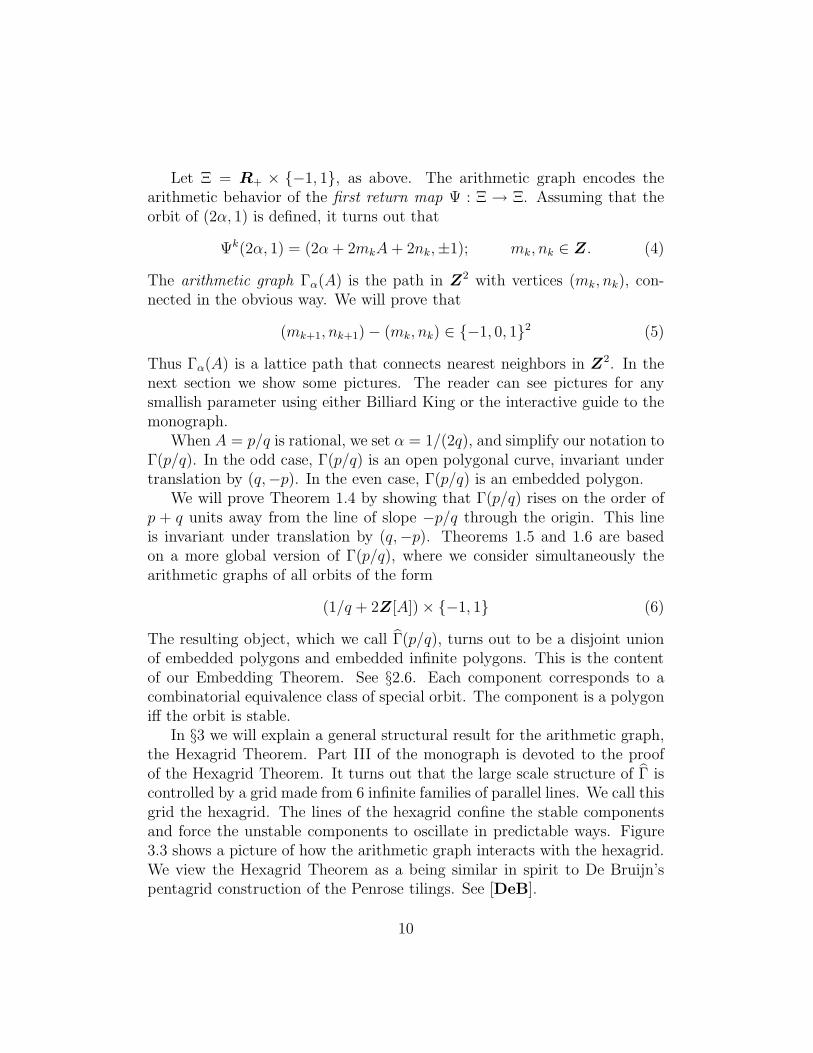
What allows us to pass from our results about rational kites, especially Theo-rem 1.4, to the results about irrational kites is a period copying phemomenon.We will illustrate the idea with some pictures. Each picture shows Γ(p/q) inreference to the line of slope −p/q through the origin. Figure 1.3 shows a bitmore than one period of Γ(7/13).

Figure 1.3: The graph Γ(7/13).

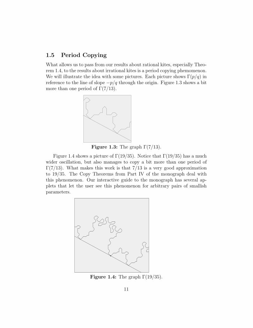
Figure 1.4 shows a picture of Γ(19/35). Notice that Γ(19/35) has a muchwider oscillation, but also manages to copy a bit more than one period ofΓ(7/13). What makes this work is that 7/13 is a very good approximationto 19/35. The Copy Theorems from Part IV of the monograph deal withthis phenomenon. Our interactive guide to the monograph has several ap-plets that let the user see this phenomenon for arbitrary pairs of smallishparameters.

Figure 1.4: The graph Γ(19/35).

11

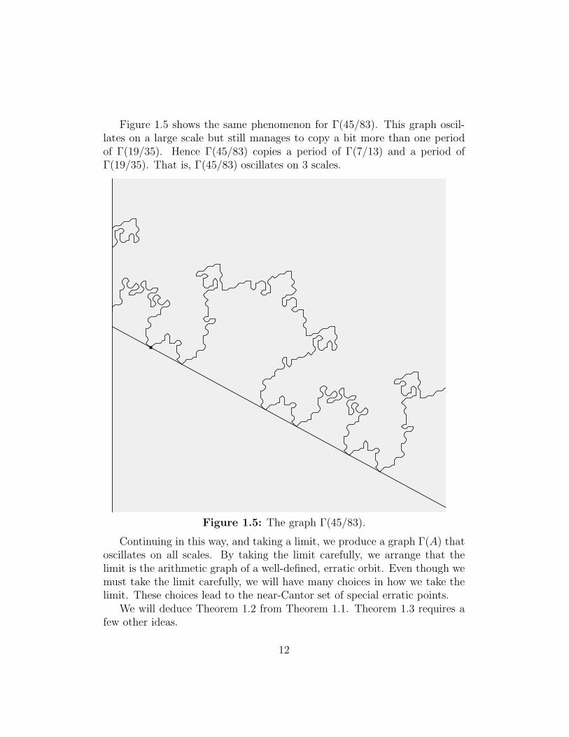
Figure 1.5 shows the same phenomenon for Γ(45/83). This graph oscil-lates on a large scale but still manages to copy a bit more than one periodof Γ(19/35). Hence Γ(45/83) copies a period of Γ(7/13) and a period ofΓ(19/35). That is, Γ(45/83) oscillates on 3 scales.

Figure 1.5: The graph Γ(45/83).

Continuing in this way, and taking a limit, we produce a graph Γ(A) thatoscillates on all scales. By taking the limit carefully, we arrange that thelimit is the arithmetic graph of a well-defined, erratic orbit. Even though wemust take the limit carefully, we will have many choices in how we take thelimit. These choices lead to the near-Cantor set of special erratic points.

We will deduce Theorem 1.2 from Theorem 1.1. Theorem 1.3 requires afew other ideas.

12

1.6 The Case of the Penrose Kite

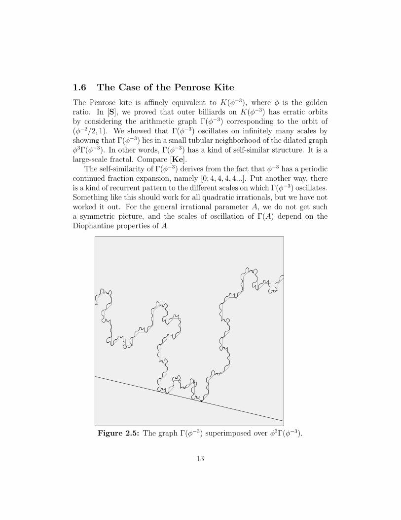
The Penrose kite is affinely equivalent to K(φ−3), where φ is the goldenratio. In [S], we proved that outer billiards on K(φ−3) has erratic orbitsby considering the arithmetic graph Γ(φ−3) corresponding to the orbit of(φ−2/2, 1). We showed that Γ(φ−3) oscillates on infinitely many scales byshowing that Γ(φ−3) lies in a small tubular neighborhood of the dilated graphφ3Γ(φ−3). In other words, Γ(φ−3) has a kind of self-similar structure. It is alarge-scale fractal. Compare [Ke].

The self-similarity of Γ(φ−3) derives from the fact that φ−3 has a periodiccontinued fraction expansion, namely [0; 4, 4, 4, 4...]. Put another way, thereis a kind of recurrent pattern to the different scales on which Γ(φ−3) oscillates.Something like this should work for all quadratic irrationals, but we have notworked it out. For the general irrational parameter A, we do not get sucha symmetric picture, and the scales of oscillation of Γ(A) depend on theDiophantine properties of A.

Figure 2.5: The graph Γ(φ−3) superimposed over φ3Γ(φ−3).

13

1.7 The Master Picture Theorem

All our main theorems follow from a combination of the Embedding Theorem,the Hexagrid Theorem, and The Copy Theorem. These three results havea common source, a result that we call the Master Picture Theorem. Weformulate and prove this result in Part II of the monograph. Here we willgive the reader a feel for the result.

Recall that Ξ = R+ × {−1, 1}. The arithmetic graph encodes the dy-namics of the first return map Ψ : Ξ→ Ξ. It turns out that Ψ is an infiniteinterval exchange map. The Master Picture Theorem reveals the followingstructure.

1. There is a locally affine map µ from Ξ into a union Ξ of two 3-dimensional tori.

2. There is a polyhedron exchange map Ψ : Ξ → Ξ, defined relative to apartition of Ξ into 28 polyhedra.

3. The map µ is a semi-conjugacy between Ψ and Ψ.

In other words, the return dynamics of Ψ has a kind of compactification intoa 3 dimensional polyhedron exchange map. All the objects above depend onthe parameter A, but we have suppressed them from our notation.

There is one master picture, a union of two 4-dimensional convex latticepolytopes partitioned into 28 smaller convex lattice polytopes, that controlseverything. For each parameter, one obtains the 3-dimensional picture bytaking a suitable slice.

The fact that nearby slices give almost the same picture is the source ofour Copy Theorem. The interaction between the map µ and the walls ofour convex polytope partitions is the source of the Hexagrid Theorem. TheEmbedding Theorem follows from basic geometric properties of the polytopeexchange map in an elementary way that is hard to summarize here.

I believe that a version of the Master Picture Theorem should hold forgeneral convex n-gons. For instance, one sees a more general picture extend-ing the one we have explained here when one considers all the orbits on akite. John Smillie and I have some ideas on how to work out the generalcase, and we hope to pursue this at a later time.

14

1.8 Computational Issues

As I mentioned above, I discovered all the structure of outer billiards byexperimenting with Billiard King. Ultimately, I am trying to verify thestructure I noticed on the computer, and so one might expect there to be somecomputation in the proof. The proof here uses considerably less computationthan the proof in [S], but I still use a computer-aided proof in several places.For example, I use the computer to check that various 4 dimensional convexintegral polytopes have disjoint interiors.

To the reader who does not like computer-aided proofs (however mild) Iwould like to remark that the experimental method here has some advantagesover a traditional proof. I checked all the main steps in the proof with massiveand visually-based computation. These checks make sure that I am not ledastray by logical or conceptual errors arising from steps taken in vacuo. Icame to the Moser-Neumann problem as a kind of blank state, and only gotthe ideas for general structural statements by looking at concrete evidence.

Again, I mention that my website has an interactive java-based guide tothis monograph. The interested reader can play with simple java appletsthat illustrate and explain many of the ideas. If nothing else, this interactiveguide provides extensive color illustrations for the monograph.

1.9 Organization of the Monograph

This monograph comes in 4 parts. In Part I, we prove all the main resultsmodulo the Hexagrid Theorem, the Embedding Theorem, the Copy Theorem,and a few smaller auxilliary results. In Part II, we prove the Master PictureTheorem. In Parts III and IV we deduce all the auxilliary theorems from theMaster Picture Theorem. Before each part of the monograph, we include anoverview of the contents of that part.

15

Part IHere is an overview of this part of the monograph.

• In §2 we define the arithmetic graph. The arithmetic graph is our mainobject of study. In this chapter, we state one key technical result aboutthe arithmetic graph, namely the Embedding Theorem. We prove theEmbedding Theorem in Part III of the monograph.

• In §3 we state our main structural result, the Hexagrid Theorem. Wethen deduce Theorems 1.4, 1.5, and 1.6 from the Hexagrid Theorem.We also deduce the Room Lemma from the Hexagrid Theorem. TheRoom Lemma is the key result needed for the proof of our main theo-rems. We prove the Hexagrid Theorem in Part III of the monograph.

• In §4 we introduce 3 more results: the Superior Sequence Lemma,Theorem 4.2 and Theorem 7.5. The first of these results deals with theapproximation of irrational numbers by odd rationals. The latter tworesults, which deal with period copying, are consequences of our CopyTheorem from Part IV. We establish the results in this chapter in PartIV.

• In §5 we prove Theorem 1.1 modulo the Embedding Theorem, theRoom Lemma, and Theorem 4.2.

• In §6 we deduce Theorem 1.2 from a geometric limit argument andTheorem 1.1.

• In §7, we prove Theorem 1.3 modulo the same technical results weassumed in the proof of Theorem 1.1, with Theorem 7.5 in place ofTheorem 4.2.

• In §8, we state some additional symmmetry properties of the Arith-metic Graph. One additional result in §8 is the Decomposition Theo-rem, a refinement of the Room Lemma, that helps us deduce Theorems4.2 and 7.5 from our general Copy Theorem. We prove the symmetryresults in Part III and the Decomposition Theorem in Part IV.

• In §9 we discuss some interesting experimental phenomena we discov-ered but have not yet proved.

16

2 The Arithmetic Graph

2.1 Polygonal Outer Billiards

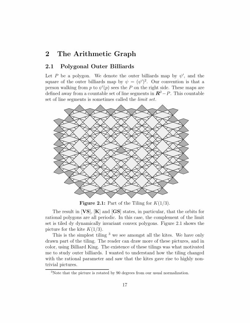
Let P be a polygon. We denote the outer billiards map by ψ′, and thesquare of the outer billiards map by ψ = (ψ′)2. Our convention is that aperson walking from p to ψ′(p) sees the P on the right side. These maps aredefined away from a countable set of line segments in R2−P . This countableset of line segments is sometimes called the limit set .

Figure 2.1: Part of the Tiling for K(1/3).

The result in [VS], [K] and [GS] states, in particular, that the orbits forrational polygons are all periodic. In this case, the complement of the limitset is tiled dy dynamically invariant convex polygons. Figure 2.1 shows thepicture for the kite K(1/3).

This is the simplest tiling 3 we see amongst all the kites. We have onlydrawn part of the tiling. The reader can draw more of these pictures, and incolor, using Billiard King. The existence of these tilings was what motivatedme to study outer billiards. I wanted to understand how the tiling changedwith the rational parameter and saw that the kites gave rise to highly non-trivial pictures.

3Note that the picture is rotated by 90 degrees from our usual normalization.

17

2.2 Special Orbits

Until the last result in this section the parameter A = p/q is rational. Saythat a special interval is an open horizontal interval of length 2/q centeredat a point of the form (a/q, b), with a odd. Here a/q need not be in lowestterms.

Lemma 2.1 The outer billiards map is entirely defined on any special inter-val, and indeed permutes the special intervals.

Proof: We note first that the order 2 rotations about the vertices of K(A)send the point (x, y) to the point:

(−2− x,−y); (−x, 2− y); (−x,−2− y); (2A− x,−y). (7)

Let ψ′ denote the outer billiards map on K(A). The map ψ′ is built outof the 4 transformations from Equation 7. The set R× Zodd is a countablecollection of lines. Let Λ ⊂ R × Zodd denote the set of points of the form(2a+2bA, 2c+1), with a, b, c ∈ Z. The complementary set Λc = R×Zodd−Λis the union of the special intervals.

Looking at Equation 7, we see that ψ′(x) ∈ Λc provided that x ∈ Λc andψ′ is defined on x. To prove this lemma, it suffices to show that ψ′ is definedon any point of Λc.

To find the points of R × Zodd where ψ′ is not defined, we extend thesides of K(A) and intersect them with R×Zodd. We get 4 families of points.

(2n, 2n+ 1); (2n,−2n− 1); (2An, 2n− 1); (2An,−2n + 1).

Here n ∈ Z. Notice that all these points lie in Λ. ♠

Let Z[A] = Z ⊕ZA. More generally, the same proof gives:

Lemma 2.2 Suppose that A ∈ (0, 1) is any number. Relative to K(A),the entire outer billiards orbit of any point (α, n) is defined provided thatα 6∈ 2Z[A] and n ∈ Zodd.

When A is irrational, the set 2Z[A] is dense in R. However, it is alwaysa countable set.

18

2.3 Structure of the Square Map

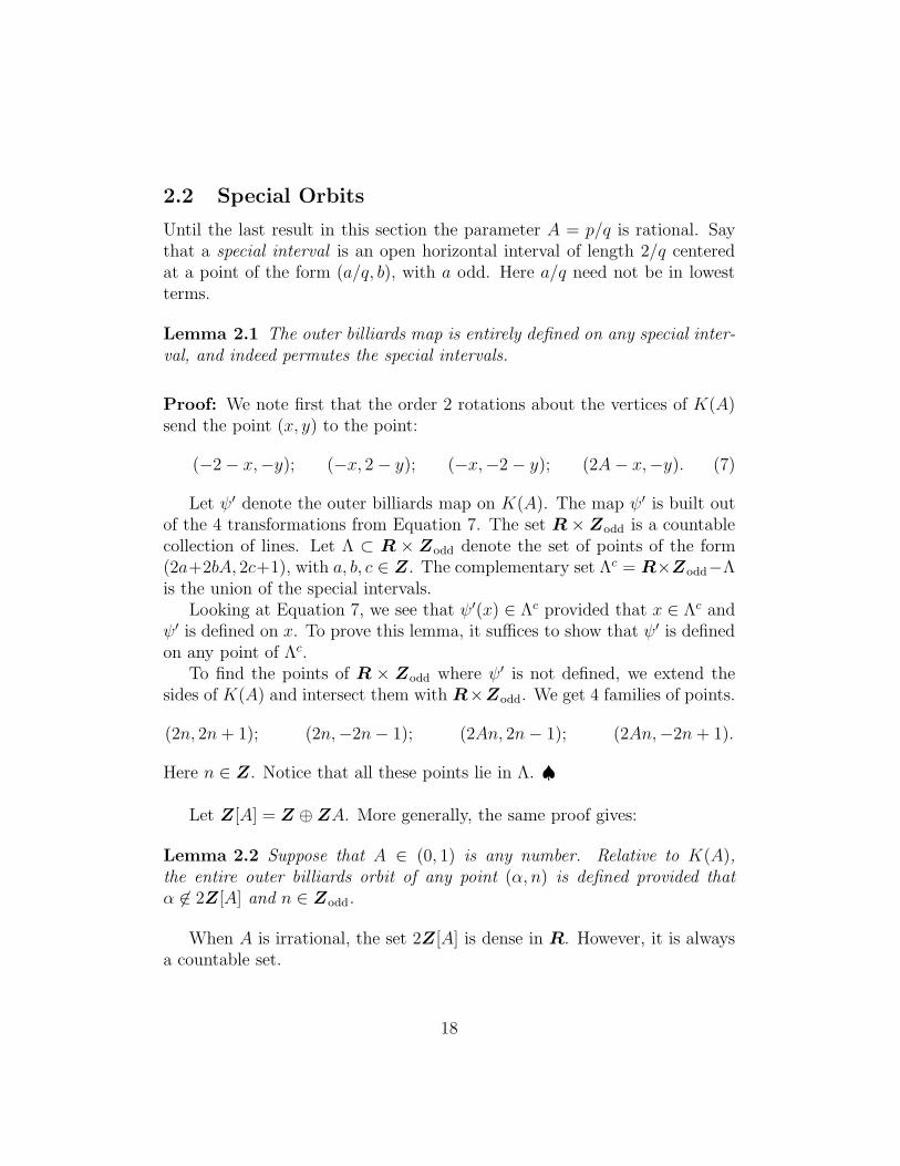
As we mentioned in §1.4, we have ψ(p) − p = V , where V is twice a vectorthat points from one vertex of K(A) to another. See Figure 1.2. There are12 possilities for V , namely

±(0, 4); ±(2, 2); ±(−2, 2); ±(2, 2A); ±(−2, 2A); ±(2 + 2A, 0). (8)

These vectors are drawn, for the parameter A = 1/3, in Figure 2.2. The greylines are present to guide the reader’s eye.

1

3

01 12

2301

03

12

1

03 23

2

0

2

Figure 2.2: The 12 direction vectors

The labelling of the vectors works as follows. We divide the plane intoits quadrants, according to the numbering scheme shown in Figure 2.2. Avector V gets the label k if there exists a parameter A and a point p ∈ Qk

such that ψ(v)− v = V . Here Qk is the kth quadrant. For instance, (0,−4)gets the labels 1 and 2. The two vectors with dots never occur. In §11.5 wewill give a much more precise version of Figure 2.2. For now, Figure 2.2 issufficient for our purposes.

19

2.4 The Return Lemma

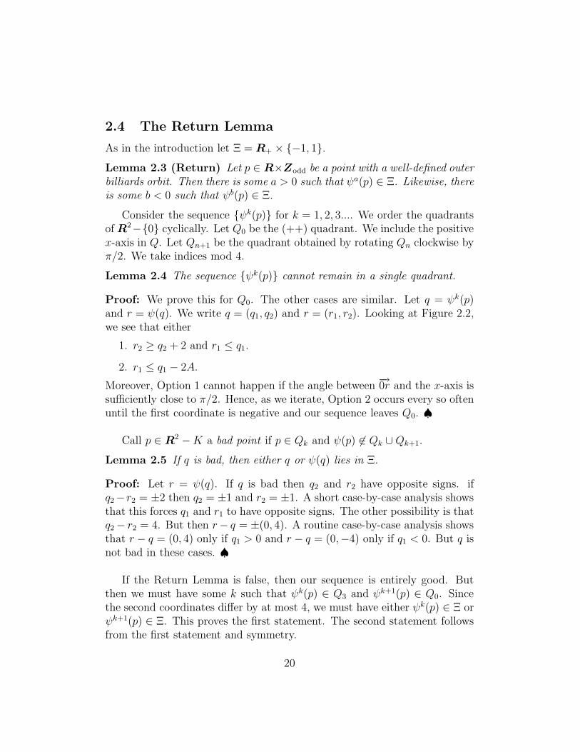
As in the introduction let Ξ = R+ × {−1, 1}.Lemma 2.3 (Return) Let p ∈ R×Zodd be a point with a well-defined outerbilliards orbit. Then there is some a > 0 such that ψa(p) ∈ Ξ. Likewise, thereis some b < 0 such that ψb(p) ∈ Ξ.

Consider the sequence {ψk(p)} for k = 1, 2, 3.... We order the quadrantsof R2−{0} cyclically. Let Q0 be the (++) quadrant. We include the positivex-axis in Q. Let Qn+1 be the quadrant obtained by rotating Qn clockwise byπ/2. We take indices mod 4.

Lemma 2.4 The sequence {ψk(p)} cannot remain in a single quadrant.

Proof: We prove this for Q0. The other cases are similar. Let q = ψk(p)and r = ψ(q). We write q = (q1, q2) and r = (r1, r2). Looking at Figure 2.2,we see that either

1. r2 ≥ q2 + 2 and r1 ≤ q1.

2. r1 ≤ q1 − 2A.

Moreover, Option 1 cannot happen if the angle between−→0r and the x-axis is

sufficiently close to π/2. Hence, as we iterate, Option 2 occurs every so oftenuntil the first coordinate is negative and our sequence leaves Q0. ♠

Call p ∈ R2 −K a bad point if p ∈ Qk and ψ(p) 6∈ Qk ∪Qk+1.

Lemma 2.5 If q is bad, then either q or ψ(q) lies in Ξ.

Proof: Let r = ψ(q). If q is bad then q2 and r2 have opposite signs. ifq2−r2 = ±2 then q2 = ±1 and r2 = ±1. A short case-by-case analysis showsthat this forces q1 and r1 to have opposite signs. The other possibility is thatq2− r2 = 4. But then r− q = ±(0, 4). A routine case-by-case analysis showsthat r − q = (0, 4) only if q1 > 0 and r − q = (0,−4) only if q1 < 0. But q isnot bad in these cases. ♠

If the Return Lemma is false, then our sequence is entirely good. Butthen we must have some k such that ψk(p) ∈ Q3 and ψk+1(p) ∈ Q0. Sincethe second coordinates differ by at most 4, we must have either ψk(p) ∈ Ξ orψk+1(p) ∈ Ξ. This proves the first statement. The second statement followsfrom the first statement and symmetry.

20

2.5 The Return Map

The Return Lemma implies that the first return map Ψ : Ξ → Ξ is welldefined on any point with an outer billiards orbit. This includes the set

(R+ − 2Z[A])× {−1, 1},

as we saw in Lemma 2.2.Given the nature of the maps in Equation 7 comprising ψ, we see that

Ψ(p)− (p) ∈ 2Z[A]× {−2, 0, 2}.

In Part II, we will prove our main structural result about the first returnmap, namely the Master Picture Theorem. We will also prove the PinwheelLemma, in Part II. Combining these two results, we have a much strongerresult about the nature of the first return map:

Ψ(p)− (p) = 2(Aǫ1 + ǫ2, ǫ3); ǫj ∈ {−1, 0, 1};3∑

j=1

ǫj ≡ 0 mod 2. (9)

Remarks:(i) Some notion of the return map is also used in [K] and [GS]. This is quitea natural object to study.(ii) We can at least roughly explain the first statement of Equation 9 in anelementary way. At least far from the origin, the square outer billiards or-bit circulates around the kite in such a way as to nearly make an octagonwith 4-fold symmetry. Compare Figure 11.3. The return pair (ǫ1(p), ǫ2(p))essentially measures the approximation error between the true orbit and theclosed octagon.(iii) On a nuts-and-bolts level, this monograph concerns how to determine(ǫ1(p), ǫ2(p)) as a function of p ∈ Ξ. (The pair (ǫ1, ǫ2) and the parity con-dition determine ǫ3.) I like to tell people that this book is really about theinfinite accumulation of small errors.(iv) Reflection in the x-axis conjugates the map ψ to the map ψ−1. Thus,once we understand the orbit of the point (x, 1) we automatically understandthe orbit of the point (x,−1). Put another way, the unordered pair of returnpoints {Ψ(p),Ψ−1(p)} for p = (x,±1) only depends on x.

21

2.6 The Arithmetic Graph

Recall that Ξ = R+ × {−1, 1}. Define M = MA,α : R× {−1, 1} by

MA,α(m,n) =(2Am+ 2m+ 2α, (−1)m+n+1

)(10)

The second coordinate of M is either 1 or −1 depending on the parity ofm+ n. This definition is adapted to the parity condition in Equation 9. Wecall M a fundamental map. Each choice of α gives a different map.

When A is irrational, M is injective. In the rational case, M is injectiveon any disk of radius q. Given p1, p2 ∈ Z2, we write p1 → p2 iff the followingholds.

• ζj = M(pj) ∈ Ξ.

• Ψ(ζ1) = ζ2.

• ‖p1 − p2‖ ≤√

2. (Compare Equation 9.)

This construction gives a directed graph with vertices in Z2. We call thisgraph the arithmetic graph and denote it by Γα(A). When A = p/q we havethe canonical choice α = 1/(2q) and then we set

Γ(p/q) = Γ1/(2q)(p/q). (11)

We say that the baseline of Γ(A) is the line M−1(0). The whole arithmeticgraph lies above the baseline. In Part III of we will prove the following result.

Theorem 2.6 (Embedding) For any A ∈ (0, 1) and α 6∈ Z[A], the graphΓα(A) is a disjoint union of embedded polygons and embedded infinite polyg-onal curves.

Remark: In the arithmetic graph, there are some lattice points having noedges emanating from them. These isolated points correspond to pointswhere the return map is the identity and hence the orbit is periodic in thesimplest possible way. We usually ignore these trivial components.

We are mainly interested in the component of Γ that contains (0, 0).We denote this component by Γ. In the rational case, Γ(p/q) encodes thestructure of the orbit O2(1/q,−1). (The orbit O2(1/q, 1), the subject ofTheorem 1.4, is conjugate to O2(1/q,−1) via reflection in the x-axis.)

In the next chapter, we will see that Γ(p/q) is a closed polygon when p/qis even, and an infinite open polygonal arc when p/q is odd.

22

3 The Hexagrid Theorem

3.1 The Arithmetic Kite

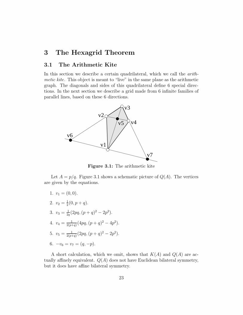
In this section we describe a certain quadrilateral, which we call the arith-metic kite. This object is meant to “live” in the same plane as the arithmeticgraph. The diagonals and sides of this quadrilateral define 6 special direc-tions. In the next section we describe a grid made from 6 infinite families ofparallel lines, based on these 6 directions.

v2

v6

v7

v3

v4

v1

v5

Figure 3.1: The arithmetic kite

Let A = p/q. Figure 3.1 shows a schematic picture of Q(A). The verticesare given by the equations.

1. v1 = (0, 0).

2. v2 = 12(0, p+ q).

3. v3 = 12q

(2pq, (p+ q)2 − 2p2).

4. v4 = 12(p+q)

(4pq, (p+ q)2 − 4p2).

5. v5 = 12(p+q)

(2pq, (p+ q)2 − 2p2).

6. −v6 = v7 = (q,−p).

A short calculation, which we omit, shows that K(A) and Q(A) are ac-tually affinely equivalent. Q(A) does not have Euclidean bilateral symmetry,but it does have affine bilateral symmetry.

23

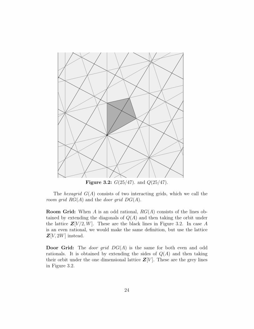
Figure 3.2: G(25/47). and Q(25/47).

The hexagrid G(A) consists of two interacting grids, which we call theroom grid RG(A) and the door grid DG(A).

Room Grid: When A is an odd rational, RG(A) consists of the lines ob-tained by extending the diagonals of Q(A) and then taking the orbit underthe lattice Z[V/2,W ]. These are the black lines in Figure 3.2. In case Ais an even rational, we would make the same definition, but use the latticeZ[V, 2W ] instead.

Door Grid: The door grid DG(A) is the same for both even and oddrationals. It is obtained by extending the sides of Q(A) and then takingtheir orbit under the one dimensional lattice Z[V ]. These are the grey linesin Figure 3.2.

24

3.2 The Hexagrid Theorem

The Hexagrid Theorem relates two kinds of objects, wall crossings and doors.Informally, the Hexagrid Theorem says that the arithmetic graph only crossesa wall at a door. Here are formal definitions.

Rooms and Walls: RG(A) divides R2 into different connected compo-nents which we call rooms. Say that a wall is the line segment of positiveslope that divides two adjacent rooms.

Doors: When p/q is odd, we say that a door is a point of intersectionbetween a wall of RG(A) and a line of DG(A). When p/q is even, we makethe same definition, except that we exclude crossing points of the form (x, y),where y is a half-integer. Every door is a triple point, and every wall hasone door. The first coordinate of a door is always an integer. (See Lemma18.2.) In exceptional cases – when the second coordinate is also an integer –the door lies in the corner of the room. In this case, we associate the doorto both walls containing it. The door (0, 0) has this property.

Crossing Cells: Say that an edge e of Γ crosses a wall if e intersects awall at an interior point. Say that a union of two incident edges of Γ crossesa wall if the common vertex lies on a wall, and the two edges point to op-posite sides of the wall. The point (0, 0) has this property. We say that acrossing cell is either an edge or a union of two edges that crosses a wallin the manner just described. For instance (−1, 1) → (0, 0) → (1, 1) is acrossing cell for any A ∈ (0, 1).

In Part III of the monograph we will prove the following result. Let ydenote the greatest integer less than y.

Theorem 3.1 (Hexagrid) Let A ∈ (0, 1) be rational.

1. Γ(A) never crosses a floor of RG(A). Any edges of Γ(A) incident to avertex contained on a floor rise above that floor (rather than below it.)

2. There is a bijection between the set of doors and the set of crossing cells.If y is not an integer, then the crossing cell corresponding to the door(m, y) contains (m, y) ∈ Z2. If y is an integer, then (x, y) correspondsto 2 doors. One of the corresponding crossing cells contains (x, y) andthe other one contains (x, y − 1).

25

Remark: We really only care about the Hexagrid Theorem when A is anodd rational. We include the even case for the sake of completeness.

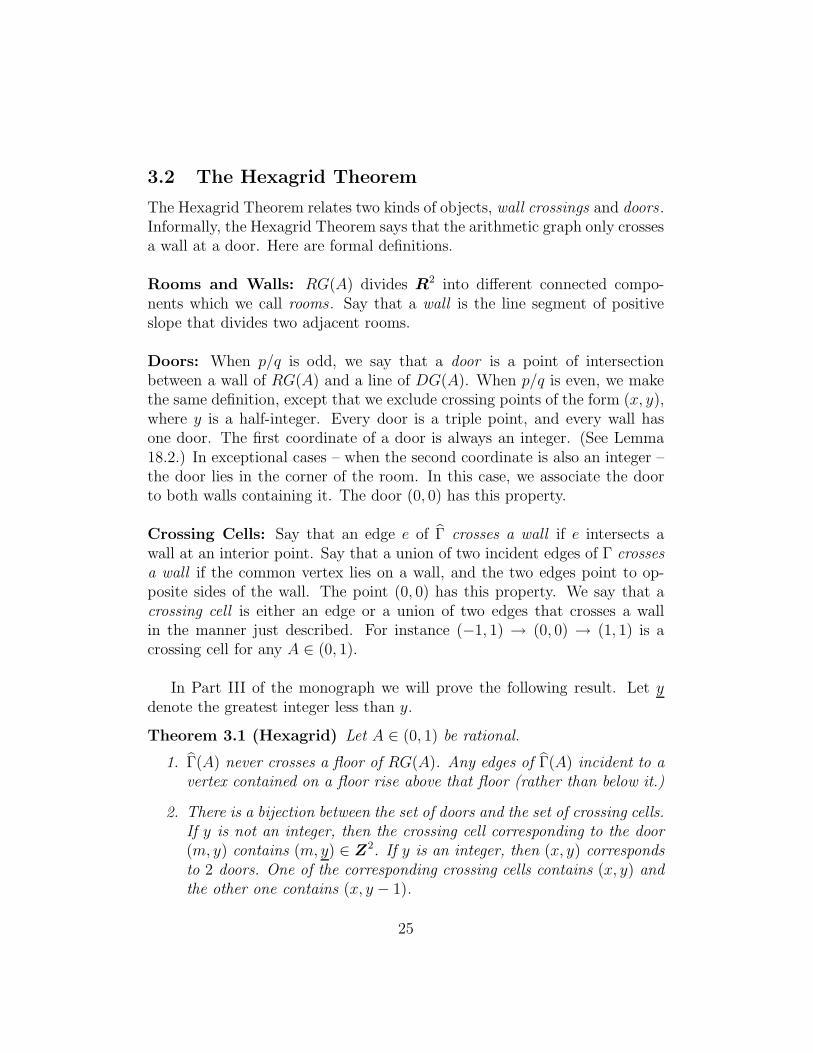
Figure 3.3 illustrates the Hexagrid Theorem for p/q = 25/47. The shadedparallelogram is R(25/47), the parallelogram from the Room Lemma below.We have only drawn the unstable components in Figure 3.3. The reader cansee much better pictures of the Hexagrid Theorem using either Billiard Kingor our interactive guide to the monograph. (The interactive guide only showsthe odd case, but Billiard King also shows the even case.)

Figure 3.3: G(25/47), R(25/47), and some of Γ(25/47).

26

3.3 The Room Lemma

For the purpose of proving our main results, we don’t need the full force of theHexagrid Theorem. All we really need is a simpler result, the Room Lemma.In this section we derive the Room Lemma from the Hexagrid Theorem.

Let p/q be an odd rational. Referring to Figure 3.1, let V = v7 andV = v3. That is,

V = (q,−p); W =(

pq

p+ q,pq

p+ q+q − p

2

). (12)

Let R(p/q) denote the parallelogram whose vertices are

(0, 0); V ; W ; V +W. (13)

R(p/q) is the shaded rectangle shown in Figure 3.3. Let

d0 = (x, y); x =p + q

2; y =

q2 − p2

4q(14)

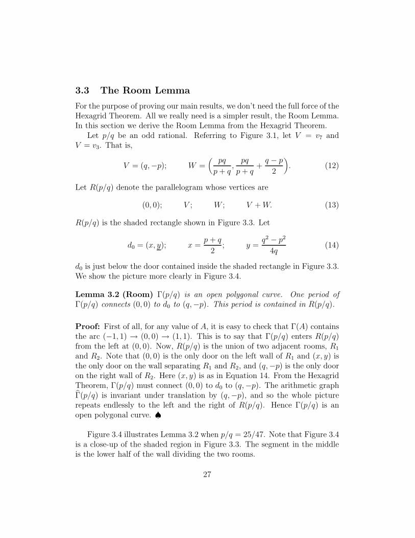
d0 is just below the door contained inside the shaded rectangle in Figure 3.3.We show the picture more clearly in Figure 3.4.

Lemma 3.2 (Room) Γ(p/q) is an open polygonal curve. One period ofΓ(p/q) connects (0, 0) to d0 to (q,−p). This period is contained in R(p/q).

Proof: First of all, for any value of A, it is easy to check that Γ(A) containsthe arc (−1, 1) → (0, 0) → (1, 1). This is to say that Γ(p/q) enters R(p/q)from the left at (0, 0). Now, R(p/q) is the union of two adjacent rooms, R1

and R2. Note that (0, 0) is the only door on the left wall of R1 and (x, y) isthe only door on the wall separating R1 and R2, and (q,−p) is the only dooron the right wall of R2. Here (x, y) is as in Equation 14. From the HexagridTheorem, Γ(p/q) must connect (0, 0) to d0 to (q,−p). The arithmetic graphΓ(p/q) is invariant under translation by (q,−p), and so the whole picturerepeats endlessly to the left and the right of R(p/q). Hence Γ(p/q) is anopen polygonal curve. ♠

Figure 3.4 illustrates Lemma 3.2 when p/q = 25/47. Note that Figure 3.4is a close-up of the shaded region in Figure 3.3. The segment in the middleis the lower half of the wall dividing the two rooms.

27

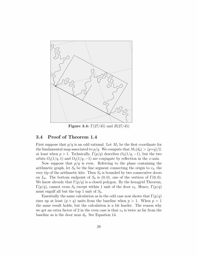
Figure 3.4: Γ(27/45) and R(27/45)

3.4 Proof of Theorem 1.4

First suppose that p/q is an odd rational. Let M1 be the first coordinate forthe fundamental map associated to p/q. We compute thatM1(d0) > (p+q)/2,at least when p > 1. Technically, Γ(p/q) describes O2(1/q,−1), but the twoorbits O2(1/q, 1) and O2(1/q,−1) are conjugate by reflection in the x-axis.

Now suppose that p/q is even. Referring to the plane containing thearithmetic graph, let S0 be the line segment connecting the origin to v3, thevery tip of the arithmetic kite. Then S0 is bounded by two consecutive doorson L0. The bottom endpoint of S0 is (0, 0), one of the vertices of Γ(0, 0).We know already that Γ(p/q) is a closed polygon. By the hexagrid Theorem,Γ(p/q), cannot cross S0 except within 1 unit of the door v3. Hence, Γ(p/q)must engulf all but the top 1 unit of S0.

Essentially the same calculation as in the odd case now shows that Γ(p/q)rises up at least (p + q) units from the baseline when p > 1. When p = 1the same result holds, but the calculation is a bit harder. The reason whywe get an extra factor of 2 in the even case is that v3 is twice as far from thebaseline as is the door near d0. See Equation 14.

28

3.5 Proof of Theorem 1.5

First suppose that p/q is odd. Let M1 be the first coordinate of the funda-mental map associated to p/q. Since p and q are relatively prime, we canrealize any integer as an integer combination of p and q. From this we seethat every point of the form s/q, with s odd, lies in the image of M1. Hence,some point of Z2, above the baseline of Γ(p/q), corresponds to the orbit ofeither (s/q, 1) or (s/q,−1).

Let the floor grid denote the lines of negative slope in the room grid.These lines all have slope −p/q. The kth line Lk of the floor grid containsthe point

ζk =(0,k(p+ q)

2

).

Modulo translation by V , the point ζk is the only lattice point on Lk. State-ment 1 of the Hexagrid Theorem contains that statement that the edges of Γincident to ζk lie between Lk and Lk+1 (rather than between Lk−1 and Lk).

We compute that

M1(ζk) = k(p+ q) +1

q.

For all lattice points (m,n) between Lk and Lk+1 we therefore have

M1(m,n) ∈ Ik, (15)

the interval from Theorem 1.5. Theorem 1.5 now follows from Equation 15,Statement 1 of the Hexagrid Theorem, and our remarks about ζk.

The proof of Theorem 1.5 in the even case is exactly the same, exceptthat we get a factor of 2 due to the different definition of the room grid.

Remark: We compare Theorem 1.5 to a result in [K]. The result in [K]is quite general, and so we will specialize it to kites. In this case, a kite isquasi-rational iff it is rational. The (special case of the) result in [K], inter-preted in our language, says that every special orbit is contained in one ofthe intervals J0, J1, J2, ..., where

Ja =p+q−1⋃

i=0

Iak+i.

The special floors corresponding to the endpoints of the J intervals corre-spond to necklace orbits. A necklace orbit (in our case) is an outer billiardsorbit consisting of copies of the kite, touching vertex to vertex. CompareFigure 2.1. Our result is a refinement in a special case.

29

3.6 Proof of Theorem 1.6

Let p/q be some rational and let Γ be the corresponding arithmetic graph.Let O2(m,n) denote the orbit corresponding to the component Γ(m,n).

Lemma 3.3 A periodic orbit O2(m,n) is stable iff Γ(m,n) is a polygon.

Proof: Let K be the period of Ψ on p0. Tracing out Γ(m,n), we get integers(mk, nk) such that

Ψk(p0)− p0 = (2mkA+ 2nk, 2ǫk); k = 1, ..., K. (16)

Here ǫk ∈ {0, 1}, and ǫk = 0 iff mk + nk is even. The integers (mk, nk)are determined by the combinatorics of a finite portion of the orbit. Hence,Equation 16 holds true for all nearby parameters A.

If Γ(m,n) is a closed polygon, then (mK , nK) = 0. But then Ψk(p0) = p0

for all parameters near A. If O2(m,n) is stable then (mK , nK) = (0, 0). Oth-erwise, the equation mKA+ nK = 0 would force A = −nK/mK . ♠

Odd Case: Assume that A = p/q is an odd rational. Say that a suite is theregion between two floors of the room grid. Each suite is partitioned intorooms. Each room has two walls, and each wall has a door in it. From theHexagrid Theorem, we see that there is an infinite polygonal arc of Γ(p/q)that lives in each suite. Let Γk(p/q) denote the infinite polygonal arc thatlies in the kth suite. With this notation Γ0(p/q) = Γ(p/q) is the componentthat contains (0, 0).

We have just described the infinite family of unstable components listedin Theorem 1.6. All the other components of Γ(p/q) are closed polygonsand must be confined to single rooms. The corresponding orbits are stable,by Lemma 3.3. The point here is that the infinite polygonal arcs we havealready described have used up all the doors. Nothing else can cross throughthe walls.

Each vertex (m,n) in the arithmetic graph corresponds to the two points(M1(m,n),±1). Thus, each component of Γ tracks either 1 or 2 orbits. Bythe parity result in Equation 9, these two points lie on different ψ-orbits.Therefore, each component of Γ tracks two special orbits. In particular,there are exactly two unstable orbits U+

k and U−

k contained in the intervalIk, and these correspond to Γk(p/q). This completes the proof in the odd case.

30

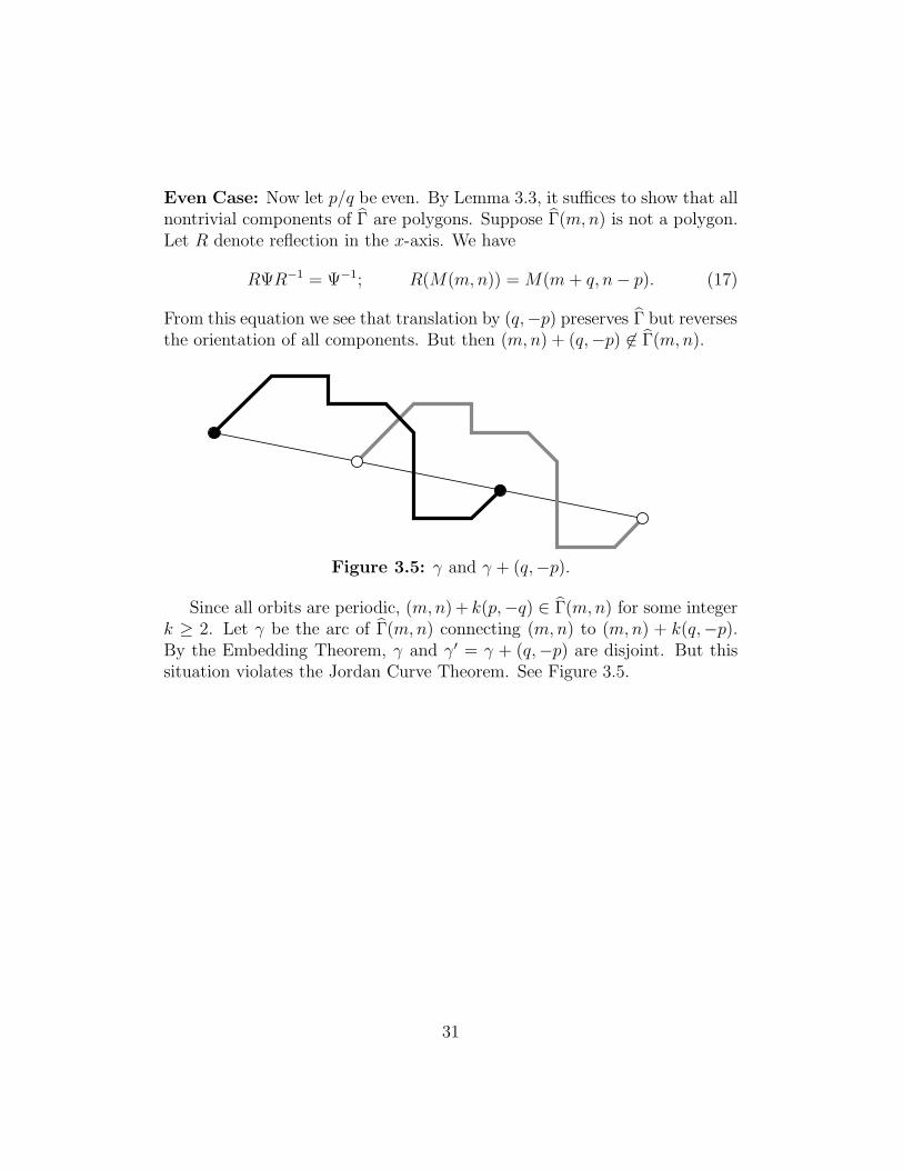
Even Case: Now let p/q be even. By Lemma 3.3, it suffices to show that allnontrivial components of Γ are polygons. Suppose Γ(m,n) is not a polygon.Let R denote reflection in the x-axis. We have

RΨR−1 = Ψ−1; R(M(m,n)) = M(m+ q, n− p). (17)

From this equation we see that translation by (q,−p) preserves Γ but reversesthe orientation of all components. But then (m,n) + (q,−p) 6∈ Γ(m,n).

Figure 3.5: γ and γ + (q,−p).

Since all orbits are periodic, (m,n) + k(p,−q) ∈ Γ(m,n) for some integerk ≥ 2. Let γ be the arc of Γ(m,n) connecting (m,n) to (m,n) + k(q,−p).By the Embedding Theorem, γ and γ′ = γ + (q,−p) are disjoint. But thissituation violates the Jordan Curve Theorem. See Figure 3.5.

31

4 Odd Approximation and Period Copying

4.1 Discussion

As we mentioned in the introduction, we would like to approximate an ir-rational A by a sequence {pn/qn} of rationals, then then study the limits ofthe corresponding arithmetic graphs Γn = Γ(pn/qn). The most obvious thingwould be to take pn/qn to be the nth continued fraction approximant of A.In this case, the arithmetic graphs Γn behave in a fairly nice way. However,when pn/qn is an even rational, the graph Γn is not so useful to us.

Here is the problem. When pn/qn is even the graph Γn is a closed polygon.The graph Γn+1 cannot copy all of Γn in this case. When pn+1/qn+1 is odd,this is easy to see: Γn+1 is an embedded open polygonal curve and hencecannot contain a closed polygon. The even case is also true, though harderto see. The interested reader can investigate the case when both pn/qn andpn+1/qn+1 are even using Billiard King.

If Γn is odd, then there is a chance that Γn+1 could copy a full periodof Γn. Thus, in order to guarantee that Γn+1 copies a full period of Γn forall n, we would need the entire sequence {pn/qn} to consist of odd rationals.This certainly does not happen for most irrational A. In §1.5 we informallydiscussed the utility of this period copying, and in the next chapter we willmake a formal argument.

We need to replace the sequence of continued fraction approximants bya related sequence consisting entirely of odd rationals. The replacementsequence is just as canonical as the sequence of continued fraction approx-imants, though it is perhaps a bit more obscure. Our sequence, which wecall the superior sequence is based on the level 2 congruence subgroup of themodular group, whereas the ordinary sequence of continued fraction approx-imants is based on the modular group itself.

One can see why the level 2 congruence subgroup might arise in thissituation. Whereas the modular group, PSL2(Z), acts in such a way as tomix up the types of rationals (odd and even) the level 2 group acts in such away as to preserve the types. The reader need not understand anything aboutthe level 2 congruence subgroup to understand our constructions. However,some readers might want to keep this connection in mind while reading ourdefinitions.

32

4.2 The Main Results

Let p/q ∈ (0, 1) be an odd rational. There are unique even rationals p+/q+and p−/q− such that

q+, q− ∈ (0, q);p−q−

<p

q<p+

q+; |pq± − qp±| = 1. (18)

If p = 1 then p− = 0. Otherwise all numbers are positive. We have thegeneral relation

p

q=p+ + p−q+ + q−

. (19)

We introduce the following notation.

p

q→ p′

q′=|p+ − p−||q+ − q−|

. (20)

We enhance our notation slightly by writing p/q ⇒ p′/q′ if q > 2q′. Here isan example.

643

1113⇒ 197

341→ 145

251→ 93

161⇒ 41

71⇒ 11

19⇒ 3

5⇒ 1

1.

Next, we write p/q =⇒ p(k)/q(k) iff we have

p(k−1)

q(k−1)⇒ p(k)

q(k).

Only this last arrow must be a double arrow. For instance, we have

643

1113=⇒ 197

341;

145

251=⇒ 11

19.

In Part IV of the monograph, we will prove the following result.

Lemma 4.1 (Superior Sequence) Let A ∈ (0, 1) be any irrational. Thenthere exists a sequence {pn/qn} such that

∣∣∣∣A−pn

qn

∣∣∣∣ <2

q2n

;pn

qn⇐=

pn+1

qn+1

∀n.

33

We call any such sequence a superior sequence. Any subsequence of asuperior sequence is also a superior sequence. By passing to a subsequence,we can take our superior sequence to be monotone. The maximal superiorsequence is unique.

Example: For the Penrose kite parameter φ−3, we obtain the maximalsuperior sequence by taking every other term in the following sequence

1

1⇐ 1

3← 1

5⇐ 3

13← 5

21⇐ 13

55← 21

89⇐ 55

233← 89

377. . .

The maximal superior sequence here obeys a linear recurrence relation sum-marized by the quadratic x2 − 4x− 1.

Let Γ = Γ(p/q) denote the arithmetic graph associated to the odd rationalp/q. Here just mean the component containing (0, 0). Let V = (q,−p), as inEquation 12. By the Room Lemma, the arc of Γ connecting (0, 0) to V is oneperiod of Γ. Call this arc Γ1. Likewise, the arc of Γ connecting (0, 0) to −Vis one period of Γ. Call this arc ⋄Γ1. So, ⋄Γ1 and Γ1 are consecutive periodsof Γ. Note that ⋄Γ1 travels leftwards from (0, 0) and Γ1 travels rightwardsfrom (0, 0). We think of the ⋄-operation as reversing the roles of left andright. Define

Γ1+ǫ = Γ1 ∪ (Bǫq(V ) ∩ Γ). (21)

Here Bǫq(V ) is the metric ball of radius ǫq about V . Intuitively, Γ1+ǫ is (1+ǫ)periods of Γ. Likewise, define

⋄Γ1+ǫ = ⋄Γ1 ∪ (Bǫq(−V ) ∩ Γ). (22)

In Part IV, we prove the following result.

Theorem 4.2 There are constants C and ǫ > 0 with the following property.Suppose p1/q1 ⇐= p2/q2 and p1 > C. Then

1. If p1/q1 < p2/q2 then Γ1+ǫ1 ⊂ Γ1

2.

2. If p1/q1 > p2/q2 then ⋄Γ1+ǫ1 ⊂ ⋄Γ1

2.

Our proof will give ǫ = 1/100, though ǫ = 1/10 is closer to the optimal.Theorem 4.2 is a consequence of our Copy Theorem, which we state andprove in Part IV.

34

4.3 A Different View of Period Copying

Here we state a variant of Theorem 4.2 that is more robust but not quiteas sharp. Let Γn denote the arc of Γ that connects (0, 0) to nV . Then Γn

consists of the first n periods of Γ. We define Γn+ǫ just as we defined Γ1+ǫ.

Theorem 4.3 There exists constants C and ǫ > 0 with the following prop-erty. Suppose that p1/q1 and p2/q2 are two odd rationals, with p1 > C and

0 <p2

q2− p1

q1<

1

(n + 1)q21

.

Then Γn+ǫ1 ⊂ Γ1

2.

Our proof gives ǫ = 1/10. There is a similar result that covers the casewhen p1/q1 > p2/q2. Theorem 4.3 is not sharp enough to imply Theorem 4.2.

Almost every A ∈ (0, 1) has the property that

0 < A− p

q<

1

2q2(23)

holds for infinitely many odd rationals. One proves this by considering theergodicity of the geodesic flow on the level 2 congruence surface.

Given such a parameter A, we can find a monotone increasing sequence{pn/qn} of odd rationals, limiting to A and satisfying the hypotheses ofTheorem 4.3 for n = 2. In this case, we have

Γ1+ǫm ⊂ Γ1

m+1; ∀m,

As we will see in the next chapter, this is all we really need to prove Theorem1.1. We mention this because Theorem 4.3 is much easier to prove thanTheorem 4.2.

The reader will find the proof of Theorem 4.3 in the first chapter of PartIV. The reader satisfied with our main results for almost every parametercan skip the rest of Part IV.

35

5 Existence of Erratic Orbits

5.1 Discussion of the Proof

Let A ∈ (0, 1) be an arbitary irrational parameter. Let {pn/qn} be a mono-tone superior sequence associated to A, as guaranteed by the Superior Se-quence Lemma. We will treat the case when this sequence is monotone in-creasing. The monotone decreasing case has essentially the same treatment.In this section we will informally explain some of the ideas in our proof.

Let Γn = Γ(pn/qn). The graph Γn corresponds to the orbit of the pointξn := (1/qn, 1). By the Room Lemma, the orbit of O2(ξn) travels on theorder of qn units away from the origin. We would like to take a kind of limit,to show that the orbit of the point ξ = lim ξn is unbounded. Unfortunately,ξ = (0, 1), a vertex of K(A). Thus, the outer billiards orbit of ξ is notdefined.

To get around this problem, we use theorem 4.2 in tandem with theRoom Lemma to show that the graph Γn has a kind of large scale Cantor setstructure. This structure implies the existence of a Cantor set C with theproperty that the orbit O2(ξn) accumulates on all of C as n→ ∞. That is,every point of C is within ǫn of a point in O2(ξn), and ǫn → 0.

Picking a generic point ξ ∈ C we will be able to find a sequence {nk}such that

ξk := ψnk(ξk)→ ξ.

Note thatO2(ξk) = O2(ξk).

On the other hand, the limit point ξ is a well defined orbit. In other words,our strategy is to look at exactly the same orbits, but to shift the indices insuch a way that the limit converges to a useful point. The sequence {nk}will diverge, but this does not bother us.

The arithmetic graph Γk corresponding to ξk is a translate of Γk. Studyingthe situation carefully, we will show that the Hausdorff limit lim Γk exists,and corresponds to an erratic orbit. Finally, we will recognize that the erraticorbit in question is O2(ξ). We have a lot of choices for ξ, and in fact we willbe able to choose ξ freely from a near-Cantor set. Thus, the special erraticset contains an essential Cantor set.

36

5.2 A Large Scale Cantor Set

Let ǫ be as in Theorem 4.2. Recall that Vn = (qn,−pn). Applying theTheorem 4.2 to every pair of consecutive terms in our superior sequence, weget

Γ1+ǫn ⊂ Γ1

n+1 ∀n. (24)

DefineΓ2

n = Γ1n + Vn+1 ⊂ Γn+1. (25)

The containment in the last equation comes from the fact that Γ1n ⊂ Γn+1

and that Γn+1 is invariant under translation by Vn+1. We take a subsequenceso that ǫqn+1 > 100qn. Then

Γ1n ⊂ Bǫqn+1

(0, 0) ∩ Γn+1. (26)

Combining Theorem 4.2 with translational symmetry and Equation 26, wehave

Γ2n ⊂ Bǫqn+1

(Vn+1) ⊂ Γ1+ǫn+1 ⊂ Γ1

n+2. (27)

In summary,

• Γ1n ⊂ Γ1

n+1 for all n.

• Γ2n = Γ1

n + Vn+1 ⊂ Γ1m for all (m,n) such that m ≥ n + 2.

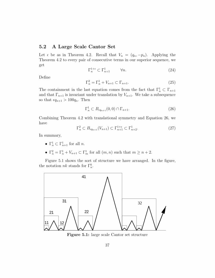
Figure 5.1 shows the sort of structure we have arranged. In the figure,the notation nk stands for Γk

n.

41

11 12

21 22

3231

Figure 5.1: large scale Cantor set structure

37

Let ǫ ∈ {0, 1}. First, we have ǫV2 ∈ Γ12 ⊂ Γ1

3. Second, for any n ≥ 1 wehave Γ1

2n−1 + ǫV2n ⊂ Γ12n+1. From these facts and induction, we have

ω(σ) :=n∑

k=1

ǫkV2k ⊂ Γ12n+1 (28)

for any binary sequence σ = ǫ1, ..., ǫn.Our next result generalizes Equation 28. For k ≤ n, we let σk denote the

sequence obtained by just switching the kth digit of σ. Let σ′k denote the

sequence obtained by setting the first k− 1 digits of σ to 0 and the kth digitto 1.

Lemma 5.1 (Translation) Let γ be the arc of Γ12k+1 connecting ω(σ) to

ω(σk). Then γ is a translation equivalent to a single period of Γ2k. Up totranslations, γ only depends on the first k digits of σ. Finally, ω(σ′

k) ⊂ γ.

Proof: We first consider the case when n = k. Our claim is independent ofthe value of the last digit of σ. So, we consider the case when σ ends in a 0and σk ends in a 1. Then γ connects the two points

ω(σ) ⊂ Γ12k−1 ⊂ Γ1

2k; ω(σk) ∈ Γ2k−1 + V2k ⊂ Γ2k ∩ Γ12k+1.

The arc Γ12k−1 + V2k starts out the second period of Γ2k. From this structure

we see that γ is exactly one period of Γ2k, and V2k = ω(σ′k) ∈ γ.

In general, let σ∗ denote the sequence obtained by setting all digits afterthe kth one to 0. Let γ∗ be the arc connecting ω(σ∗) to ω(σ∗

k). Then, bythe special case we have already considered, γ∗ is one period of Γ2k andγ∗ ⊂ Γ1

2k+1. By an inductive argument, we establish that

γ∗ +n∑

j=k+1

ǫjV2j ⊂ Γ12n+1.

But the arc on the left hand side of this equation connects ω(σ) to ω(σk),and hence equals γ, the arc of interest to us. In short

γ = γ∗ +n∑

j=k+1

ǫjV2j . (29)

Equation 29 combines with the special case we have already considered toestablish the lemma. ♠

38

5.3 Taking a Limit

Our limit construction is based on any infinite binary sequence σ = {ǫn}with infinitely many 0s and infinitely many 1s. Let σ(n) denote the first ndigits of σ. For k < n, let σk(n) denote the sequence obtained from σ(n) byswitching the kth digit. Let ω(n) = ω(σ(n)) and ωk(n) = ω(σk(n)).

Let N = 2n+ 1. Define

Γ′

n = ΓN − ω(n). (30)

Note that Γ′n is the arithmetic graph for the point ζn = MN(ω(n)). Here MN

is the fundamental map associated to pN/qN . (See Equation 35 below.)

Lemma 5.2 There are divergent sequences {E0n} and {E1n} such that thefirst E0n edges of Γ′

m in the forwards direction are independent of m ≥ nand the first E1n edges of Γ′

m in the backwards direction are independent ofm ≥ n.

Proof: Let γk be the arc connecting ω(n) to ωk(n). By the TranslationLemma, the arc γ′k = γk − ωn connecting 0 to ωk(n) − ω(n) belongs to Γ′

n

and is independent of n > k. For each n, we let ni < n be the largest placewhere the nith digit of σ is an i. Let Ein denote the number of edges in γ′ni

.These sequences do the job. ♠

Lemma 5.2 implies that the graphs {Γ′n} converge to a limiting graph Γ∞.

We want to control the rate of this convergence. Here are 4 basic definitions.

• Let LN denote the baseline of ΓN . Let

L′

n = LN − ω(n) (31)

• Let Bn denote the ball of radius 2 max(E0n, E1n) about 0. Note thatthe first E0n forwards edges of Γ∞ lie in Bn and the first E1n backwardsedges of Γ∞ lie in Bn.

• Let dn denote the distance from ω(n) to LN . Note that dn is also thedistance from 0 to L′

n.

• Define M0(m,n) = 2Am + n. Here M0 is the linear part of the firstcoordinate of any fundamental map associated to the parameter A.

39

Passing to a subsequence we can arrange the following.

• M0(Vn) < 10−n.

• |dm − dn| < 10−n for all m > n.

• |An −Am| < 10−n for all m > n.

• The limit L∞ = limL′n exists, and L′

n ∩ Bn lies within 10−n of L∞.

Only the last item requires some explanation. The size of Bn is at mostO(q2n) whereas the slope of L′

n differs from the slope of L∞ by O(q−22n ).

Lemma 5.3 Γ∞ rises unboundedly far away from L∞ in either direction.

Proof: The point d0 in Lemma 3.2 lies at least q/4 units above the base-line. Hence, by Lemma 3.2, the arc γ0n rises at least q2n0

/4 units above LN .Hence, the first E0n forward edges of Γ′

n rise at least q2n0/4 above L′

n. Hence,the first E0n forward edges of Γ∞ rise at least q2n0

/4 − 1 above L∞. Thebackwards direction is similar. ♠

Lemma 5.4 Both directions of Γ∞(σ) come arbitrarily close to L∞.

Proof: M0 maps L∞ to a single point, namely

M0(L∞) = −∞∑

n=1

ǫjM0(V2n). (32)

By the last statement of the Translation Lemma, the arc γ′n0⊂ Γ∞ contains

a vertex of the form

µn = ω(σ′

k(n))− ω(σ(n)) = −n0∑

i=1

ǫnV2n +∞∑

n=n0+1

ǫ′nV2n. (33)

Here {ǫ′n} is a binary sequence whose composition is irrelevant. We thereforehave

|M0(L∞)−M0(Vn)| <∞∑

n=n0+1

M(V2n) < 2× 10−n0.

This last equation does the job for us. ♠

40

5.4 Recognizing the Limit

Referring to our sequence σ = {ǫi}, define

ξ =( ∞∑

n=1

ǫjM0(V2n),−1). (34)

Our rapid decay rates imply that this limit exists and that the map σ → ξ(σ)is injective. Hence, our construction produces uncountably many choices ofξ. Throwing out a countable set, we choose so that the first coordinate doesnot lie in 2Z[A]. In this case, the outer billiards orbit of ξ is well definedrelative to K(A).

Lemma 5.5 Γ∞ is the arithmetic graph of ξ and L∞ is the baseline of Γ∞.

Proof: Recall that N = 2n+1. Let MN be the fundamental map associatedto ΓN . That is,

MN (x, y) = 2ANx+ 2y +1

qN. (35)

For any lattice point (x, y), the first coordinate of MN(x, y) converges toM0(x, y) as n → ∞. Let ξn = MN(ωn). By construction, ξn → ξ. As wealready remarked, Γ′

n is the arithmetic graph for ξn, relative to AN .Let O2(ξn;N) denote the outer billiards orbit of ξn relative to K(AN ).

Since ξn → ξ and AN → A and O2(ξ) is defined, the graph Γ′n describes

O2(ξ) on increasingly large balls. Taking the limit, we see that Γ∞ is thearithmetic graph corresponding to O2(ξ). We have M0(L∞) = −ξ by Equa-tion 32. Let M be the fundamental map such that M(0, 0) = ξ. The firstcoordinate of M differs from M0 by the addition of ξ. Hence, the first coor-dinate of M maps L∞ to 0. Hence L∞ is the baseline for Γ∞. ♠

The last two results in the previous section show that (ξ, 1) lies in the spe-cial erratic set. Given that our construction works for any binary sequencehaving infinitely many 0s and 1s, we see that the special erratic set containsa near-Cantor set. This completes the proof of Theorem 1.1, modulo sometechnical details.

Terminology: Since ξ 6∈ 2Z[A], the entire arithmetic graph Γ∞ is defined.We call this graph a limit graph. The component of Γ∞ through (0, 0),namely Γ∞, is the one we analyzed in this chapter.

41

6 The Orbit Dichotomy

6.1 An Easy Case of the Result

Before we prove Theorem 1.2 in general, we prove a special case that hasmany of the features of the general case. Recall that Ξ = R+×{−1, 1}. Wewill suppose that B ∈ Ξ has an aperiodic but bounded forward orbit. Wewill also suppose that there is an erratic orbit E ∈ Ξ such one and the samearithmetic graph has a component corresponding to B and a componentcorresponding to E. Essentially, this means that the first coordinate of Bdiffers from the first coordinate of E by an element of 2Z[A].

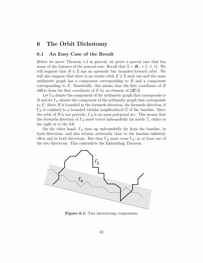
Let ΓB denote the component of the arithmetic graph that corresponds toB and let ΓE denote the component of the arithmetic graph that correspondsto E. Since B is bounded in the forwards direction, the forwards direction ofΓB is confined to a bounded tubular neighborhood Σ of the baseline. Sincethe orbit of B is not periodic, ΓB is an open polygonal arc. This means thatthe forwards direction of ΓB must travel unboundedly far inside Σ, either tothe right or to the left.

On the other hand, ΓE rises up unboundedly far from the baseline, inboth directions, and also returns arbitrarily close to the baseline infinitelyoften and in both directions. But then ΓB must cross ΓE , in at least one ofthe two directions. This contradicts the Embedding Theorem.

EΓ

BΓ

Figure 6.1: Two intersecting components

42

6.2 The Main Argument

Now we suppose that B ∈ R×Zodd is a point with a well defined aperiodicorbit that is bounded in, say, the forwards direction. By the Return Lemma,it suffices to take B ∈ Ξ.

Given an arithmetic graph Γ and a point β ∈ Z2, let Γ(β) denote thecomponent of Γ that contains β. The translated arithmetic graph Γ(β)− βcontains the origin. In the next section we will establish the following result.

Lemma 6.1 (Rigidity) Let {An} be any sequence of parameters converg-ing to an irrational parameter A. Let Γn denote any sequence of arithmeticgraphs, such that Γn is based on An. Let βn denote a lattice point that liesabove the baseline Ln of Γn. Suppose that the distance from βn to Ln con-verges to 0. Then the sets Γn(βn) − βn converge in the Hausdorff topology.The limit Γ0 only depends on A. Indeed, Γ0 is the Hausdorff limit of thegraphs Γ(pn/qn), where {pn/qn} is any sequence of rationals converging to A.

We will use the Rigidity Lemma for the proof of Theorem 1.3. All weneed for the proof of Theorem 1.2 is the following corollary.

Corollary 6.2 Let A be an irrational parameter. Let Γ be some arithmeticgraph associated to A. Let βn denote a lattice point that lies above the baselineL of Γ. Suppose that the distance from βn to L converges to 0. Then the setsΓ(βn)−βn converge in the Hausdorff topology. The limit Γ0 rises unboundedlyfar from L.

Proof: The only statement that is not immediate is the last statement. Forthe last statement, we consider the graphs Γn from the proof of Theorem1.1. The limit of these graphs rises unboundedly far from the baseline, inone direction or the other, because this limit contains a period of each Γn. ♠

ΓB has the same structure as considered in the special case above. Sincethe baseline L has irrational slope, we can find a sequence of points βn ∈ Z2

such that βn lies above the baseline L, but the distance from βn to L convergesto 0. Taking a Hausdorff limit of the graphs Γ(βn)− βn, we get a limit thatrises unboundedly far from L, by Corollary 6.2. But this shows, for k large,Γ(βk). starts out beneath ΓB and rises up through the strip Σ. But now wecontradict the Embedding Theorem, as in the special case.

43

6.3 Proof of The Rigidity Lemma

Given any A ∈ (0, 1) and ǫ > 0, let Σǫ(A) ⊂ (0, 1)2 denote those pairs (s, A′)where s ∈ (0, ǫ) and |A′ − A| < ǫ. Let O(s, 1;A′) denote the outer billiardsorbit of (s, 1) relative to K(A′).

Lemma 6.3 Suppose that A ∈ (0, 1) is irrational. For any N there is someǫ > 0 with the following property. The first N iterates of O(s, 1;A′), forwardsand backwards, are well defined provided that (s, A′) ∈ Σǫ(A).

Proof: Inspecting the proof of Lemma 2.1, we draw the following conclusion.If O(s, 1;A′) is not defined after N iterates, then s = 2A′m+ 2n for integersm,n ∈ (−N ′, N ′). Here N ′ depends only on N . Rearranging this equation,we get

|A′ − m

n| < s

2m.

For s sufficiently small and A′ sufficiently close to A, this is impossible. ♠

Lemma 6.4 Suppose that A ∈ (0, 1) is irrational. For any N there is someǫ > 0 with the following property. The combinatorics of the first N forwarditerates of O(s, 1;A′) is independent of the choice of point (s, A′) ∈ Σǫ(A).The same goes for the first N backwards iterates.

Proof: This follows from the fact that the combinatorial type, a discretepiece of data, varies continuously over any region where all N iterates aredefined. ♠

Corollary 6.5 There is a divergent sequence {nk} with the following prop-erty. If |A − A′| < 1/k and s, s′ ∈ (0, 1/k), then the first nk forwards (orbackwards) iterates of O(s, 1;A) have the same combinatorial structure as thefirst nk forwards (or backwards) iterates of O(s′, 1;A′).

Let Ψ denote the first return map relative to the parameter A. Likewisedefine Ψ′. The following result is just a consequence of the existence of thereturn map. See the Return Lemma from §2.

44

Corollary 6.6 There is a divergent sequence {Nk} with the following prop-erty. If |A − A′| < 1/k and s, s′ ∈ (0, 1/k), then the first Nk iterates of Ψapplied to (s, 1) have the same combinatorial structure as the first Nk iter-ates of Ψ′ applied to (s′, 1). This holds in both the forwards and backwardsdirections.

The Hausdorff distance between two compact sets S1, S2 ⊂ R2 is the in-fimal d = d(S1, S2) such that S1 us contained in the d tubular neighborhoodof S2, and vice versa. A sequence {Sn} of closed sets in R2 converges in theHausdorff topology if there is a closed subset S such that d(Sn∩K,S∩K)→ 0for every compact K.

Proof of the Rigidity Lemma: The existence of a universal limit Γ0 is justa reformulation of the preceding corollary. the point is that the arithmeticgraph exactly captures the combinatorial structure of the return map. Sincethe limit Γ0 is independent of which sequence of graphs/points we choose,we let Γn = Γ(pn/qn) and we let βn = (0, 0) for all n. ♠

We include one more result, which will be useful in the next chapter.

Lemma 6.7 For any n there is a vertex v of Γ0 such that ‖v‖ > n and v iswithin 1/n of the line of slope −A through 0.

Proof: Let {pn/qn} denote our final sequence considered in §7. We haveΓ1

n ⊂ Γ1m for all m > n. Taking the limit, we see that vn = (qn,−pn) ∈ Γ0 for

all n. These points serve our purpose. (In the case not treated in our proofof Theorem 1.1, we would have Γ0

n ⊂ Γ0m for all m > n. Here Γ0

n = Γ1n − vn.

In this case, the points −vn would all belong to Γ0.) ♠

45

7 The Density of Periodic Orbits

7.1 Topological Orbit Confinement

The Embedding Theorem tells us that Γα(A) is an disjoint union of embed-ded polygons and infinite embedded polygonal arcs. This fact gives us atopological method for producing periodic orbits. There are two methods.

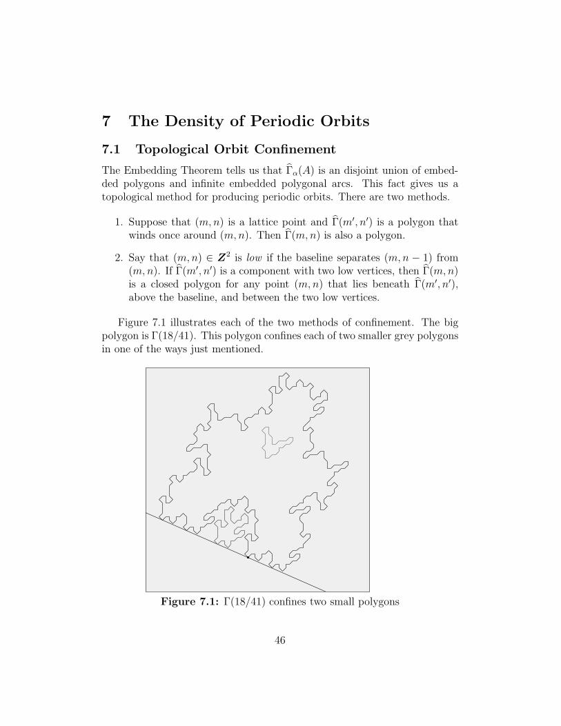
1. Suppose that (m,n) is a lattice point and Γ(m′, n′) is a polygon thatwinds once around (m,n). Then Γ(m,n) is also a polygon.

2. Say that (m,n) ∈ Z2 is low if the baseline separates (m,n − 1) from(m,n). If Γ(m′, n′) is a component with two low vertices, then Γ(m,n)is a closed polygon for any point (m,n) that lies beneath Γ(m′, n′),above the baseline, and between the two low vertices.

Figure 7.1 illustrates each of the two methods of confinement. The bigpolygon is Γ(18/41). This polygon confines each of two smaller grey polygonsin one of the ways just mentioned.

Figure 7.1: Γ(18/41) confines two small polygons

46

7.2 Main Argument

We define the depth of a lattice point (above the baseline) to be the distancefrom this lattice point to the baseline of Γ. We define the depth of a polygonin Γ to be the minimum of the depth of its vertices. In this section, weprove the following result. Let Γ denote some limit graph associated to theparameter A.

Lemma 7.1 Suppose that Γ contains a sequence {γk} of polygon componentssuch that the depth of γk tends to 0. Then the set of special periodic orbitsrelative to K(A) is dense in the set of all special periodic orbits.

Let |γk| denote the supremal value of d such that there are two verticesof γk, at least d apart, having depth less than 1/d.

Lemma 7.2 |γk| → ∞ as k →∞.

Proof: Let (mk, nk) be the vertex of γk of lowest depth. By the Rigid-ity Lemma, the component γk − (mk, nk) converges to Γ0, and one directionor the other connects (mk, nk) to a far away and low-depth vertex (m′

k, n′k). ♠

Let Sk denote the set of components γ′ of Γ such that γ′ is translationequivalent to γk and the corresponding vertices are low. The vertex (m,n)is low if the baseline of Γ separates (m,n) and (m,n− 1).

Lemma 7.3 There is some constant Nk so that every point of L is withinNk units of a member of Sk.

Proof: Say that a lattice point (m,n) is very low if it has depth less than1/100 (but still positive.) The polygon γk corresponds to a periodic orbitξk. Since ξk is periodic, there is an open neighborhood Uk of ξk such that allorbits in Uk are combinatorially identical to ξk. Let M be fundamental mapassociated to Γ. Then M−1(Uk) is an open strip, parallel to L. Since L hasirrational slope, there is some constant Nk so that every point of L is withinNk of some point of M−1(Uk) ∩ Z2. But the components of Γ containingthese points are translation equivalent to γk. Choosing Uk small enough, wecan guarantee that the translations taking γk to the other components carrythe very low vertices of γk to low vertices. ♠

47

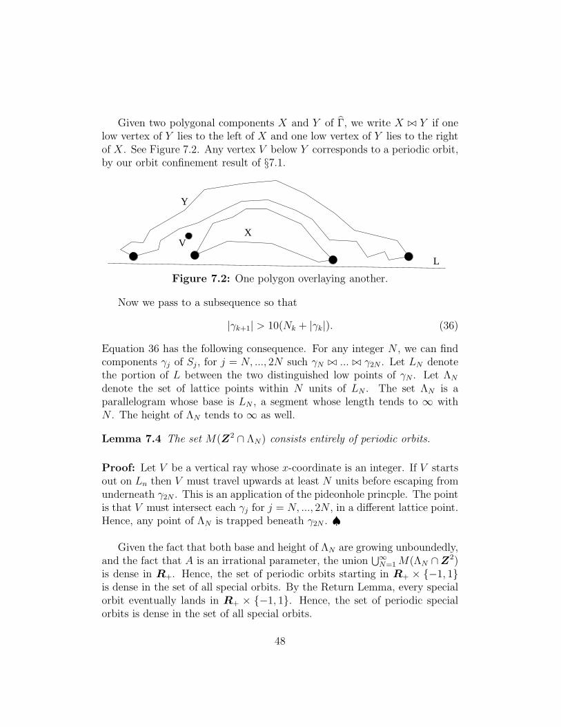
Given two polygonal components X and Y of Γ, we write X ⊲⊳ Y if onelow vertex of Y lies to the left of X and one low vertex of Y lies to the rightof X. See Figure 7.2. Any vertex V below Y corresponds to a periodic orbit,by our orbit confinement result of §7.1.

L

Y

VX

Figure 7.2: One polygon overlaying another.

Now we pass to a subsequence so that

|γk+1| > 10(Nk + |γk|). (36)

Equation 36 has the following consequence. For any integer N , we can findcomponents γj of Sj , for j = N, ..., 2N such γN ⊲⊳ ... ⊲⊳ γ2N . Let LN denotethe portion of L between the two distinguished low points of γN . Let ΛN

denote the set of lattice points within N units of LN . The set ΛN is aparallelogram whose base is LN , a segment whose length tends to ∞ withN . The height of ΛN tends to ∞ as well.

Lemma 7.4 The set M(Z2 ∩ ΛN) consists entirely of periodic orbits.

Proof: Let V be a vertical ray whose x-coordinate is an integer. If V startsout on Ln then V must travel upwards at least N units before escaping fromunderneath γ2N . This is an application of the pideonhole princple. The pointis that V must intersect each γj for j = N, ..., 2N , in a different lattice point.Hence, any point of ΛN is trapped beneath γ2N . ♠

Given the fact that both base and height of ΛN are growing unboundedly,and the fact that A is an irrational parameter, the union

⋃∞

N=1M(ΛN ∩Z2)is dense in R+. Hence, the set of periodic orbits starting in R+ × {−1, 1}is dense in the set of all special orbits. By the Return Lemma, every specialorbit eventually lands in R+ × {−1, 1}. Hence, the set of periodic specialorbits is dense in the set of all special orbits.

48

7.3 The Cap Construction

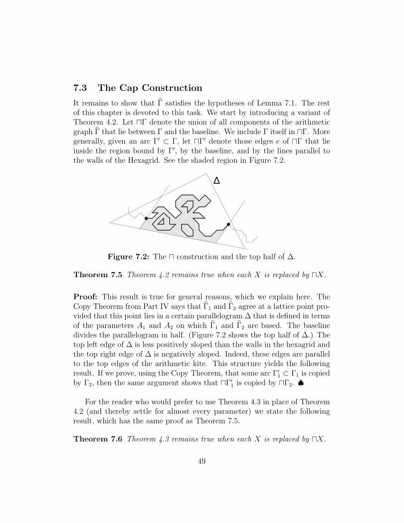
It remains to show that Γ satisfies the hypotheses of Lemma 7.1. The restof this chapter is devoted to this task. We start by introducing a variant ofTheorem 4.2. Let ⊓Γ denote the union of all components of the arithmeticgraph Γ that lie between Γ and the baseline. We include Γ itself in ⊓Γ. Moregenerally, given an arc Γ′ ⊂ Γ, let ⊓Γ′ denote those edges e of ⊓Γ that lieinside the region bound by Γ′, by the baseline, and by the lines parallel tothe walls of the Hexagrid. See the shaded region in Figure 7.2.

∆

Figure 7.2: The ⊓ construction and the top half of ∆.

Theorem 7.5 Theorem 4.2 remains true when each X is replaced by ⊓X.

Proof: This result is true for general reasons, which we explain here. TheCopy Theorem from Part IV says that Γ1 and Γ2 agree at a lattice point pro-vided that this point lies in a certain parallelogram ∆ that is defined in termsof the parameters A1 and A2 on which Γ1 and Γ2 are based. The baselinedivides the parallelogram in half. (Figure 7.2 shows the top half of ∆.) Thetop left edge of ∆ is less positively sloped than the walls in the hexagrid andthe top right edge of ∆ is negatively sloped. Indeed, these edges are parallelto the top edges of the arithmetic kite. This structure yields the followingresult. If we prove, using the Copy Theorem, that some arc Γ′

1 ⊂ Γ1 is copiedby Γ2, then the same argument shows that ⊓Γ′

1 is copied by ⊓Γ2. ♠

For the reader who would prefer to use Theorem 4.3 in place of Theorem4.2 (and thereby settle for almost every parameter) we state the followingresult, which has the same proof as Theorem 7.5.

Theorem 7.6 Theorem 4.3 remains true when each X is replaced by ⊓X.

49

7.4 Manufacturing the Periodic Sequence

In the next section we prove the following key result.

Lemma 7.7 Let p/q be any odd rational. Then O2(3/q, 1) 6= O2(1/q,±1).

Let Γ′n denote the component of Γn = Γ(pn/qn) that contains the vertex

corresponding to the orbit of (3/qn, 1).

Lemma 7.8 Γ′n is a polygon.

Proof: Note that Γ′n 6= Γn, by Lemma 7.7. Theorem 1.6 now implies that

O(3/qn, 1) is stable. Hence Γ′n is a polygon. Alternatively, Γ′

n contains a lowvertex and hence lies beneath Γn. Hence, Γn confines Γ′

n. ♠

We constructed the limit graph Γ from a superior sequence {An} wewill suppose that this sequence is monotone increasing. The other case hasessentially the same proof. Note that Γ′

n ⊂ ⊓Γ1n. Note also that Γ′

n has avertex ζn within 3/qn of the baseline.

Lemma 7.9 ⊓Γ contains translates of ⊓Γ1n for n sufficiently large.

Proof: First let’s prove that Γ contains translates of Γ1n for n large. Refer-

ring to the proof of Lemma 5.4, the portion of the arc γ′n0starting at the

point µn and travelling to the right contains a translate of Γ1k for an infinite

number of indices k. Also Γ1n contains Γ1

k−1. Hence Γ contains translates ofΓ1

n for all n. To get the result with ⊓X in place of X, we use Theorem 7.5 inplace of Theorem 4.2. All the relevant constructions in §5 go through wordfor word. ♠

By the previous result, there is a translation τn such that

γn := τn(Γ′

n) ⊂ τn(⊓Γ1n) ⊂ ⊓Γ ⊂ Γ (37)

Our proof of Lemma 7.9 gives us the additional piece of information that thedistance from τn(0, 0) to the baseline of Γ converges to 0 with n.

Given that |An−A| < 2q−2n and ‖ζn− (0, 0)‖ < C(qn) for some universal

constnt, we see that the same result holds for τn(ζn) Hence, the depth of γn

tends to 0 as n tends to ∞. This shows that Γ satisfies the hypotheses ofLemma 7.1. This completes the proof of Theorem 1.3, modulo Lemma 7.7.

50

7.5 Proof of Lemma 7.7

We assume that p > 1. Suppose O2(3/q, 1) = O2(1/q, 1). Then Ψk(3/q, 1) =(1/q, 1) for some k. But then

(2/q, 0) = (3/q, 1)−Ψk(3/q, 1) = (2m(p/q) + 2n, 0); m+ n even

The parity result comes from Equation 9. Equating the first coordinates andclearing denominators, we get 1 = mp+ nq. This is impossible for p/q odd.

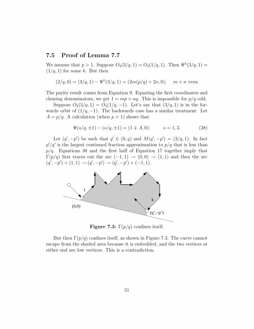
Suppose O2(3/q, 1) = O2(1/q,−1). Let’s say that (3/q, 1) is in the for-wards orbit of (1/q,−1). The backwards case has a similar treatment. LetA = p/q. A calculation (when p > 1) shows that

Ψ(s/q,±1)− (s/q,±1) = (1∓ A, 0); s = 1, 3. (38)

Let (q′,−p′) be such that q′ ∈ (0, q) and M(q′,−p′) = (3/q, 1). In factp′/q′ is the largest continued fraction approximation to p/q that is less thanp/q. Equations 38 and the first half of Equation 17 together imply thatΓ(p/q) first traces out the arc (−1, 1) → (0, 0) → (1, 1) and then the arc(q′,−p′) + (1, 1)→ (q′,−p′)→ (q′,−p′) + (−1, 1).

(0,0)

1

(q’,−p’)

k

Figure 7.3: Γ(p/q) confines itself.

But then Γ(p/q) confines itself, as shown in Figure 7.3. The curve cannotescape from the shaded area because it is embedded, and the two vertices ateither end are low vertices. This is a contradiction.

51

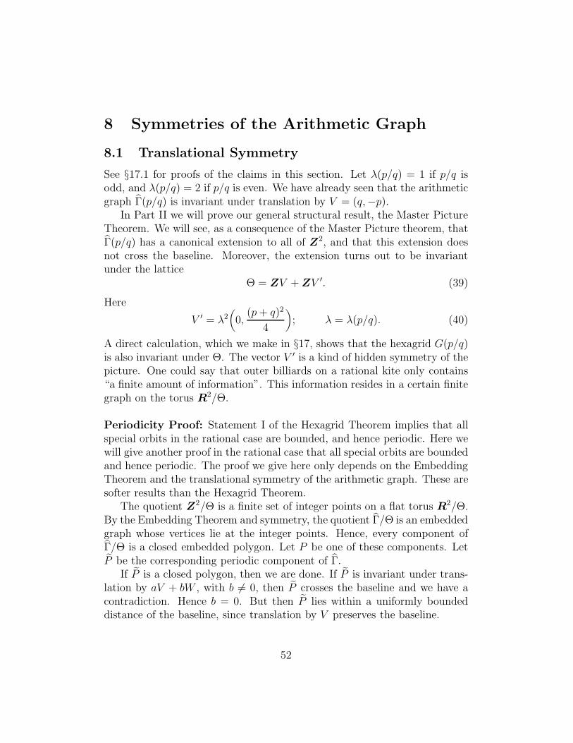
8 Symmetries of the Arithmetic Graph

8.1 Translational Symmetry

See §17.1 for proofs of the claims in this section. Let λ(p/q) = 1 if p/q isodd, and λ(p/q) = 2 if p/q is even. We have already seen that the arithmeticgraph Γ(p/q) is invariant under translation by V = (q,−p).

In Part II we will prove our general structural result, the Master PictureTheorem. We will see, as a consequence of the Master Picture theorem, thatΓ(p/q) has a canonical extension to all of Z2, and that this extension doesnot cross the baseline. Moreover, the extension turns out to be invariantunder the lattice

Θ = ZV + ZV ′. (39)

Here

V ′ = λ2(0,

(p+ q)2

4

); λ = λ(p/q). (40)

A direct calculation, which we make in §17, shows that the hexagrid G(p/q)is also invariant under Θ. The vector V ′ is a kind of hidden symmetry of thepicture. One could say that outer billiards on a rational kite only contains“a finite amount of information”. This information resides in a certain finitegraph on the torus R2/Θ.

Periodicity Proof: Statement I of the Hexagrid Theorem implies that allspecial orbits in the rational case are bounded, and hence periodic. Here wewill give another proof in the rational case that all special orbits are boundedand hence periodic. The proof we give here only depends on the EmbeddingTheorem and the translational symmetry of the arithmetic graph. These aresofter results than the Hexagrid Theorem.

The quotient Z2/Θ is a finite set of integer points on a flat torus R2/Θ.By the Embedding Theorem and symmetry, the quotient Γ/Θ is an embeddedgraph whose vertices lie at the integer points. Hence, every component ofΓ/Θ is a closed embedded polygon. Let P be one of these components. LetP be the corresponding periodic component of Γ.

If P is a closed polygon, then we are done. If P is invariant under trans-lation by aV + bW , with b 6= 0, then P crosses the baseline and we have acontradiction. Hence b = 0. But then P lies within a uniformly boundeddistance of the baseline, since translation by V preserves the baseline.

52

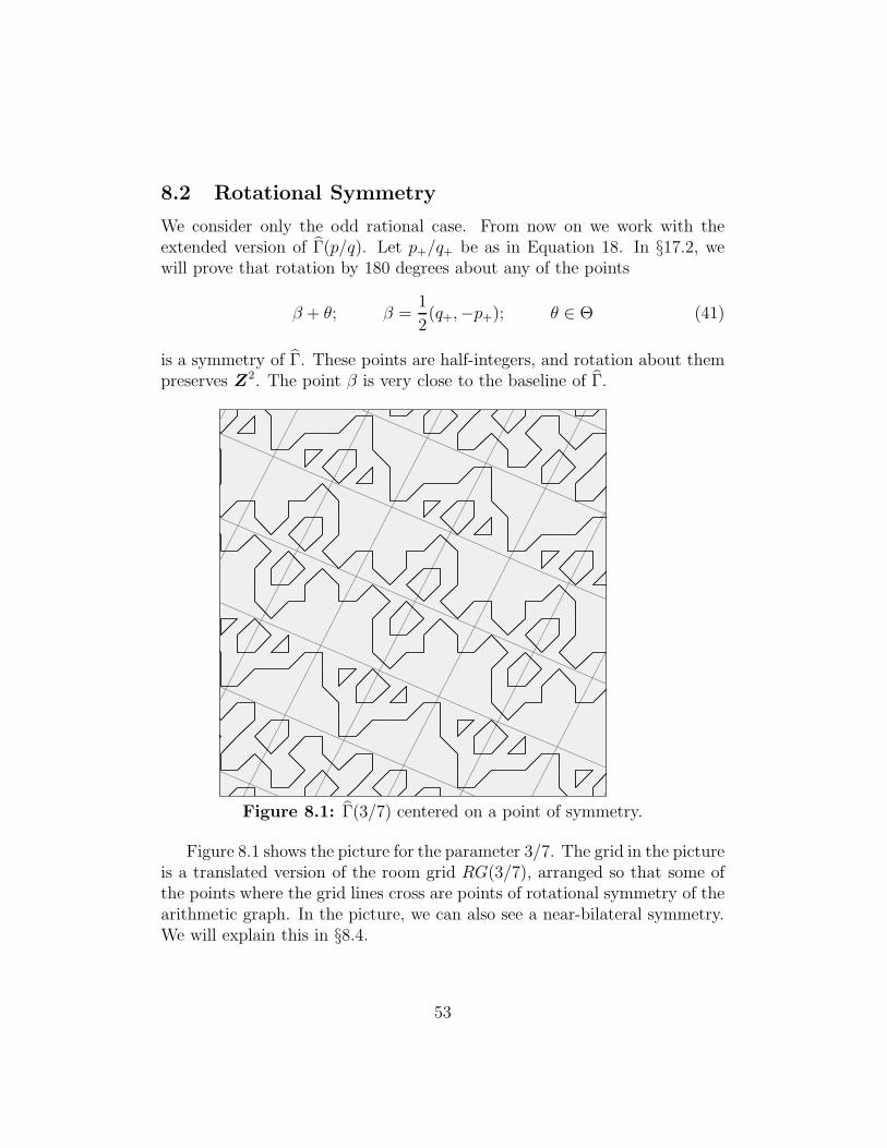
8.2 Rotational Symmetry

We consider only the odd rational case. From now on we work with theextended version of Γ(p/q). Let p+/q+ be as in Equation 18. In §17.2, wewill prove that rotation by 180 degrees about any of the points

β + θ; β =1

2(q+,−p+); θ ∈ Θ (41)

is a symmetry of Γ. These points are half-integers, and rotation about thempreserves Z2. The point β is very close to the baseline of Γ.

Figure 8.1: Γ(3/7) centered on a point of symmetry.

Figure 8.1 shows the picture for the parameter 3/7. The grid in the pictureis a translated version of the room grid RG(3/7), arranged so that some ofthe points where the grid lines cross are points of rotational symmetry of thearithmetic graph. In the picture, we can also see a near-bilateral symmetry.We will explain this in §8.4.

53

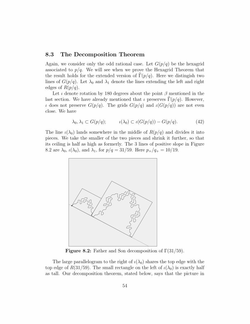
8.3 The Decomposition Theorem

Again, we consider only the odd rational case. Let G(p/q) be the hexagridassociated to p/q. We will see when we prove the Hexagrid Theorem thatthe result holds for the extended version of Γ(p/q). Here we distingish twolines of G(p/q). Let λ0 and λ1 denote the lines extending the left and rightedges of R(p/q).

Let ι denote rotation by 180 degrees about the point β mentioned in thelast section. We have already mentioned that ι preserves Γ(p/q). However,ι does not preserve G(p/q). The grids G(p/q) and ι(G(p/q)) are not evenclose. We have

λ0, λ1 ⊂ G(p/q); ι(λ0) ⊂ ι(G(p/q))−G(p/q). (42)

The line ι(λ0) lands somewhere in the middle of R(p/q) and divides it intopieces. We take the smaller of the two pieces and shrink it further, so thatits ceiling is half as high as formerly. The 3 lines of positive slope in Figure8.2 are λ0, ι(λ0), and λ1, for p/q = 31/59. Here p+/q+ = 10/19.

Figure 8.2: Father and Son decomposition of Γ(31/59).

The large parallelogram to the right of ι(λ0) shares the top edge with thetop edge of R(31/59). The small rectangle on the left of ι(λ0) is exactly halfas tall. Our decomposition theorem, stated below, says that the picture in

54

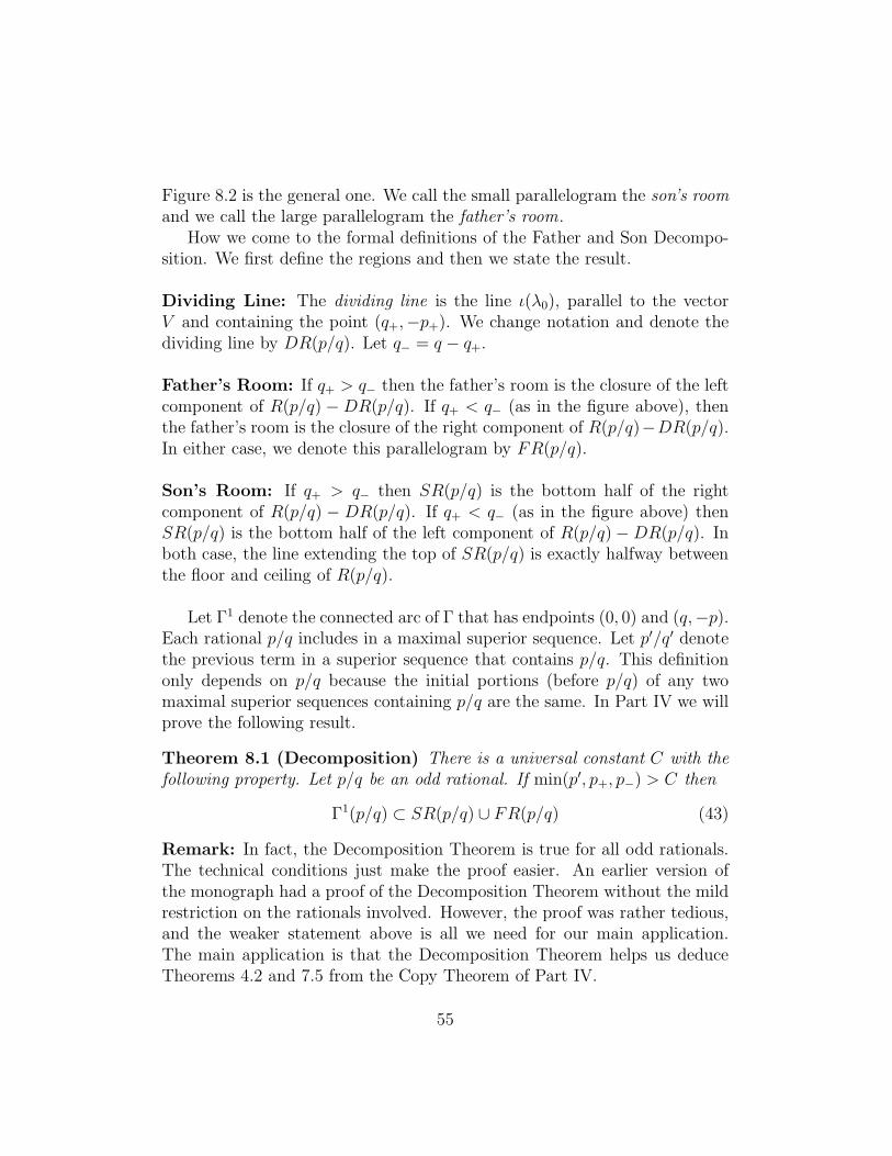
Figure 8.2 is the general one. We call the small parallelogram the son’s roomand we call the large parallelogram the father’s room.

How we come to the formal definitions of the Father and Son Decompo-sition. We first define the regions and then we state the result.

Dividing Line: The dividing line is the line ι(λ0), parallel to the vectorV and containing the point (q+,−p+). We change notation and denote thedividing line by DR(p/q). Let q− = q − q+.

Father’s Room: If q+ > q− then the father’s room is the closure of the leftcomponent of R(p/q) −DR(p/q). If q+ < q− (as in the figure above), thenthe father’s room is the closure of the right component of R(p/q)−DR(p/q).In either case, we denote this parallelogram by FR(p/q).

Son’s Room: If q+ > q− then SR(p/q) is the bottom half of the rightcomponent of R(p/q) − DR(p/q). If q+ < q− (as in the figure above) thenSR(p/q) is the bottom half of the left component of R(p/q)−DR(p/q). Inboth case, the line extending the top of SR(p/q) is exactly halfway betweenthe floor and ceiling of R(p/q).

Let Γ1 denote the connected arc of Γ that has endpoints (0, 0) and (q,−p).Each rational p/q includes in a maximal superior sequence. Let p′/q′ denotethe previous term in a superior sequence that contains p/q. This definitiononly depends on p/q because the initial portions (before p/q) of any twomaximal superior sequences containing p/q are the same. In Part IV we willprove the following result.

Theorem 8.1 (Decomposition) There is a universal constant C with thefollowing property. Let p/q be an odd rational. If min(p′, p+, p−) > C then

Γ1(p/q) ⊂ SR(p/q) ∪ FR(p/q) (43)

Remark: In fact, the Decomposition Theorem is true for all odd rationals.The technical conditions just make the proof easier. An earlier version ofthe monograph had a proof of the Decomposition Theorem without the mildrestriction on the rationals involved. However, the proof was rather tedious,and the weaker statement above is all we need for our main application.The main application is that the Decomposition Theorem helps us deduceTheorems 4.2 and 7.5 from the Copy Theorem of Part IV.

55

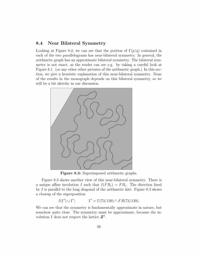
8.4 Near Bilateral Symmetry

Looking at Figure 8.2, we can see that the portion of Γ(p/q) contained ineach of the two parallelograms has near-bilateral symmetry. In general, thearithmetic graph has an approximate bilateral symmetry. The bilateral sym-metry is not exact, as the reader can see e.g. by taking a careful look atFigure 8.1. (or any other other pictures of the arithmetic graph.) In this sec-tion, we give a heuristic explanation of this near-bilateral symmetry. Noneof the results in the monograph depends on this bilateral symmetry, so wewill be a bit sketchy in our discussion.

Figure 8.3: Superimposed arithmetic graphs.

Figure 8.3 shows another view of this near-bilateral symmetry. There isa unique affine involution I such that I(FR1) = FR1. The direction fixedby I is parallel to the long diagonal of the arithmetic kite. Figure 8.3 showsa closeup of the superposition

I(Γ′) ∪ Γ′; Γ′ = Γ(73/139)∩ FR(73/139).

We can see that the symmetry is fundamentally approximate in nature, butsomehow quite close. The symmetry must be approximate, because the in-volution I does not respect the lattice Z2.

56

Let M(m,n) = ξ ∈ R+ denote the point corresponding to the latticepoint (m,n). Here M is the fundamental map associated to the parameterp/q. The forwards ψ orbit of (m,n, 1) winds halfway around the kite andthen encounters a point of the form

(2Am′ + 2n′,±1) ∈ R− × {−1, 1}.

The lattice point (m,n) lies above the baseline of Γ(p/q) and the latticepoint (m′, n′) lies below the baseline. Given the geometry of the return mapΨ, as discussed in detail in §11, the points (m,n) and (m′, n′) lie about thesame distance from the baseline. Indeed, a calculation shows that there is auniformly small constant C such that

‖(m′, n′)− J(m,n)‖ < C,

where J is the affine involution fixing the baseline and mapping the linesextending R(p/q) to themselves. We could probably take C = 2.

We define J∗(m,n) = (m′, n′). We might have based J∗ on the orbitof (2Am + 2n,−1), but the result would be uniformly close. In any case,J∗ maps components of Γ above the baseline to components of Γ below thebaseline, in such a way that the corresponding components are uniformlyclose to having the same affine shape. The map J∗ does not quite induce acombinatorial isomorphism on each component. J∗ would map two vertices(m1, n1) and (m2, n2) to the same point if

(m1, n1, 1)→ ...→ (m′, n′, 1); (m2, n2, 1)→ ...→ (m; , n′,−1)

under iteration of the map ψ.Letting ι denote the 180 degree rotation about the point β from Equation

41, the map β ◦ J∗ maps Γ(p/q) to itself and is uniformly close to the affineinvolution I discussed in connection with Figure 8.3. Indeed, up to a tinytranslational discrepancy, we have I = β ◦ J .

In terms of Figure 8.1, the maps β and J generate the dihedral symmetrygroup of the grid, fixing the center point. The maps β and J∗ generate anorder 4 group of permutations of the components of Γ(p/q).

57

9 Further Results and Conjectures

In this chapter we will state some conjectures, and also a few additionalresults. Mainly we include the results to motivate the conjectures and insome case provide support for them. Our proofs of these results will bepretty sketchy.

9.1 Return Dynamics

In this section we will consider the full outer billiards orbit, and not just theorbit under the square map. We say that an orbit is forwards erratic if theforwards direction is unbounded and also enters every neighborhood of thekite vertex set. We define backwards erratic orbits in the same way. Theorem1.1 implies that outer billiards on any irrational kite has uncountably manyorbits that are erratic simultaneously in both directions.

Let X = (0, 2)× {±1}. The orbits in X seem to have a particularly nicestructure. Given a Cantor set C ⊂ X, let C ′ denote the set of endpoints ofthe components of X − C.

Conjecture 9.1 Let A ∈ (0, 1) be an irrational parameter. Then there is aCantor set CA ⊂ X with the following properties relative to outer billiardson K(A).

1. An orbit of X is well-defined iff it lies in X − C ′A.

2. All the orbits in X−CA are periodic. Orbits within the same componentof X − CA have the same combinatorial structure as each other.

3. Each orbit of CA−C ′A is unbounded, and intersects CA in a dense set.

4. All but one orbit of CA − C ′A is forwards erratic and all but one orbit

of CA − C ′A is backwards erratic.

In [S] we essentially proved Statements 3 and 4 for the Penrose kiteparameter A = φ−3.

We don’t know much about the orbits that don’t start in X, but here isone conjecture. Let U ⊂ R×Zodd be union of all points that have unboundedorbits.

Conjecture 9.2 Any unbounded special orbit is dense in U , and erratic inat least one direction.

58

9.2 Low Components

Recall that a lattice point (m,n) is low with respect to the parameter p/qif the baseline of Γ(p/q) separates (m,n − 1) from (m,n). Such verticescorrespond to points in X. We say that a low component of Γ(p/q) is acomponent that contains a low vertex. The basic idea behind Conjecture 9.1is that the low components have a structure that (conjecturally) is built upinductively from the continued fraction expansion of the parameter. In thissection we explore this structure.

Now that we are talking about the arithmetic graph again, we revert backto the study of the square of the outer billiards map.

Conjecture 9.3 Let p/q be any rational. Two low vertices (m1, n1) and(m2, n2) lie on the same component of Γ(p/q) only if m1 + n1 and m2 + n2

have the same parity.

We will sketch the proof in the odd case.

Lemma 9.4 Let A ∈ (0, 1) be any parameter, and let s0, s1 ∈ (0, 2) be anypoints on which the outer billiards orbits are defined. Then

O2(s0, 1) 6= O2(s1,−1).

Proof: (sketch) Let Γ be the arithmetic graph corresponding to the commonorbit O2(s0, 1) = O2(s1,−1). Let (mj , nj) denote the vertex corresponding tosj. Then (mj, nj) is a low vertex. The line segment σj connecting (mj , nj−1)to (mj , nj) crosses the baseline of Γ. As Γ′ passes (mj , nj), the segment σj

is either on the right or the left, relative to the canonical orientation on Γ′.An explicit calculation shows that σj is on the right for j = 0 and on the leftfor j = 1. But then we get the same topological contradiction that we got inthe proof of Lemma 7.7. ♠

The first half of the proof of Lemma 7.7 combines with Lemma 9.4 toestablish Conjecture 9.3 in the odd case. Lemma 9.4 generalizes the argumentwe gave in the second half of the proof of Lemma 7.7

We don’t know how to prove Conjecture 9.3 in the even case.In general, the low components of Γ(p/q) seem to be built up from the

low components of Γ(p′/q′) for simpler rational p′/q′ that approximate p/q.

59

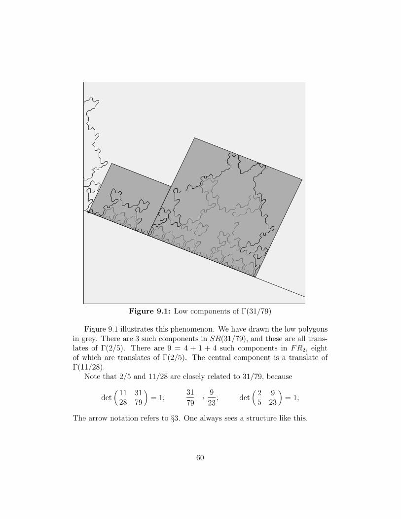
Figure 9.1: Low components of Γ(31/79)

Figure 9.1 illustrates this phenomenon. We have drawn the low polygonsin grey. There are 3 such components in SR(31/79), and these are all trans-lates of Γ(2/5). There are 9 = 4 + 1 + 4 such components in FR2, eightof which are translates of Γ(2/5). The central component is a translate ofΓ(11/28).

Note that 2/5 and 11/28 are closely related to 31/79, because

det(

11 3128 79

)= 1;

31

79→ 9

23; det

(2 95 23

)= 1;

The arrow notation refers to §3. One always sees a structure like this.

60

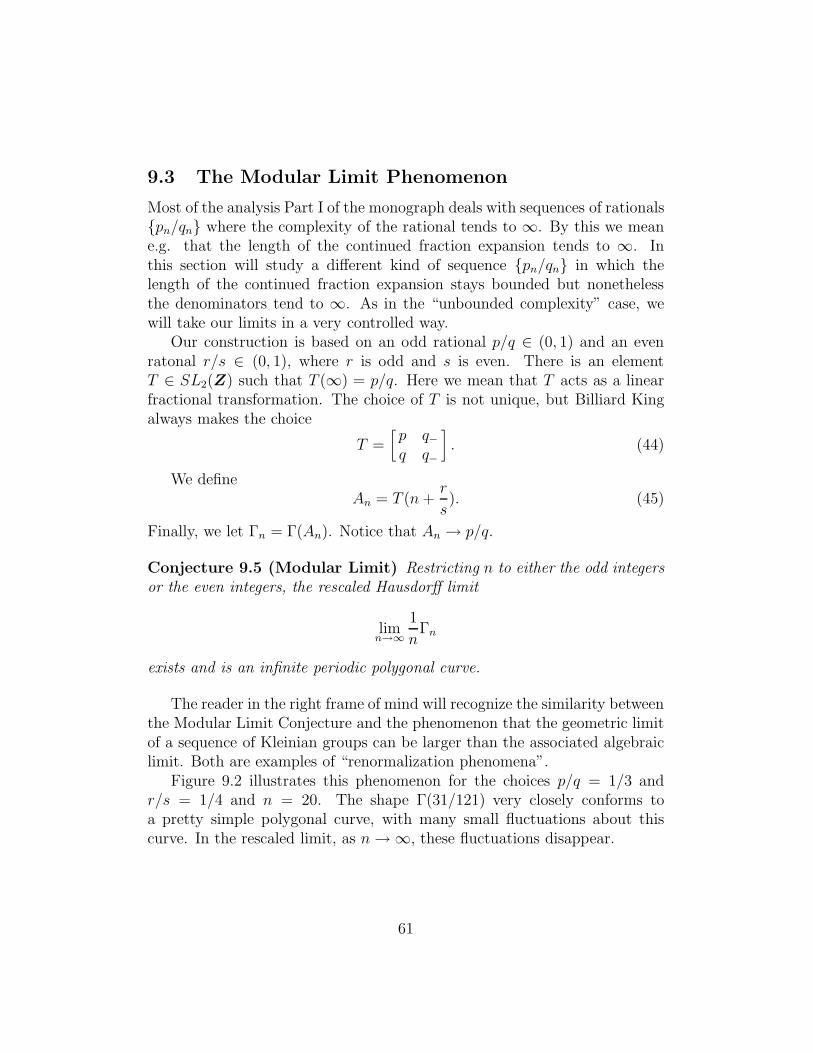
9.3 The Modular Limit Phenomenon

Most of the analysis Part I of the monograph deals with sequences of rationals{pn/qn} where the complexity of the rational tends to ∞. By this we meane.g. that the length of the continued fraction expansion tends to ∞. Inthis section will study a different kind of sequence {pn/qn} in which thelength of the continued fraction expansion stays bounded but nonethelessthe denominators tend to ∞. As in the “unbounded complexity” case, wewill take our limits in a very controlled way.

Our construction is based on an odd rational p/q ∈ (0, 1) and an evenratonal r/s ∈ (0, 1), where r is odd and s is even. There is an elementT ∈ SL2(Z) such that T (∞) = p/q. Here we mean that T acts as a linearfractional transformation. The choice of T is not unique, but Billiard Kingalways makes the choice

T =[p q−q q−

]. (44)

We defineAn = T (n+

r

s). (45)

Finally, we let Γn = Γ(An). Notice that An → p/q.

Conjecture 9.5 (Modular Limit) Restricting n to either the odd integersor the even integers, the rescaled Hausdorff limit

limn→∞

1

nΓn

exists and is an infinite periodic polygonal curve.

The reader in the right frame of mind will recognize the similarity betweenthe Modular Limit Conjecture and the phenomenon that the geometric limitof a sequence of Kleinian groups can be larger than the associated algebraiclimit. Both are examples of “renormalization phenomena”.

Figure 9.2 illustrates this phenomenon for the choices p/q = 1/3 andr/s = 1/4 and n = 20. The shape Γ(31/121) very closely conforms toa pretty simple polygonal curve, with many small fluctuations about thiscurve. In the rescaled limit, as n→∞, these fluctuations disappear.

61

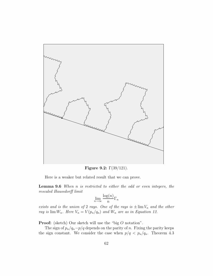
Figure 9.2: Γ(39/121).

Here is a weaker but related result that we can prove.

Lemma 9.6 When n is restricted to either the odd or even integers, therescaled Haussdorff limit

limn→∞

log(n)

nΓn

exists and is the union of 2 rays. One of the rays is ± limVn and the otherray is limWn. Here Vn = V (pn/qn) and Wn are as in Equation 12.

Proof: (sketch) Our sketch will use the “big O notation”.The sign of pn/qn−p/q depends on the parity of n. Fixing the parity keeps

the sign constant. We consider the case when p/q < pn/qn. Theorem 4.3

62

forces the forwards direction of Γn to copy O(n) periods of Γ(p/q). When thisportion is rescaled at a sublinear rate, it converges to the forward directionof the baseline, namely limVn.

Recall that the behavior of Γn is controlled not just by the hexagrid Gn

but also a rotated copy of Gn. See the discussion in §8.3. It turns out thatthere are 2 line segments σ1 and σ2 with the following properties.

• σ1 and σ2 are both parallel to Wn and have length O(n).

• σ1 and σ2 are O(1) units apart from each other.

• The first O(n) steps of the backwards portion of Γn are contained be-tween σ1 and σ2.

σ1 is the left edge of the rectangle Rn = R(pn/qn) and σ2 is the parallelsegment containing the point (−q, p)/2. So, the backwards direction of Γn

travels up O(n) steps up a uniformly narrow strip. When rescaled at a sub-linear rate, the result converges to limWn. ♠

Both Billiard King and the interactive guide to the monograph are set upso that the reader can explore this phenomenon and variants. One interestingvariant arises when we take p/q to be even. In this case, the limit above seemsto contain solid triangular pieces. Figure 9.3 below shows an example of this,for the parameter 101/200, a very close approximation to 1/2.

Here is a weaker but more concrete formulation, which we have no ideahow to prove.

Conjecture 9.7 The limit

limn→∞

log(n)

nΓn

exists and is the union of two cones in R2.

When p/q is extremely near an even rational, Γ(p/q) exhibits some plane-filling tendencies. We have no idea why this happens. All we can say thatΓn can’t copy a full period of Γ(p/q) because Γn is embedded and Γ(p/q) isa closed polygon. So, something else is forced to happen.

63

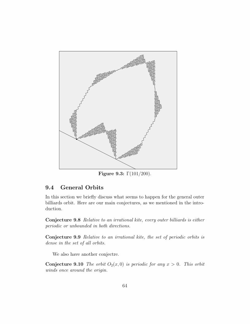
Figure 9.3: Γ(101/200).

9.4 General Orbits

In this section we briefly discuss what seems to happen for the general outerbilliards orbit. Here are our main conjectures, as we mentioned in the intro-duction.

Conjecture 9.8 Relative to an irrational kite, every outer billiards is eitherperiodic or unbounded in both directions.

Conjecture 9.9 Relative to an irrational kite, the set of periodic orbits isdense in the set of all orbits.

We also have another conjectre.

Conjecture 9.10 The orbit O2(x, 0) is periodic for any x > 0. This orbitwinds once around the origin.

64

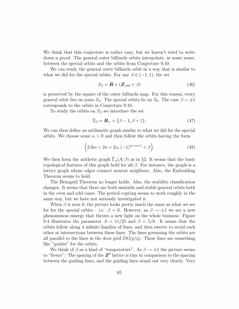
We think that this conjecture is rather easy, but we haven’t tried to writedown a proof. The general outer billiards orbits interpolate, in some sense,between the special orbits and the orbits from Conjecture 9.10.

We can study the general outer billiards orbit in a way that is similar towhat we did for the special orbits. For any β ∈ (−1, 1), the set

Sβ = R× (Zodd + β) (46)

is preserved by the square of the outer billiards map. For this reason, everygeneral orbit lies on some Sβ. The special orbits lie on S0. The case β = ±1corresponds to the orbits in Conjecture 9.10.

To study the orbits on Sβ we introduce the set

Ξβ = R+ × {β − 1, β + 1}. (47)

We can then define an arithmetic graph similar to what we did for the specialorbits. We choose some α > 0 and then follow the orbits having the form

(2Am+ 2n+ 2α, (−1)m+n+1 + β

). (48)

We then form the arithetic graph Γα(A; β) as in §2. It seems that the basictopological features of this graph hold for all β. For instance, the graph is alattice graph whose edges connect nearest neighbors. Also, the EmbeddingTheorem seems to hold.

The Hexagrid Theorem no longer holds. Also, the stability classificationchanges. It seems that there are both unstable and stable general orbits bothin the even and odd cases. The period copying seems to work roughly in thesame way, but we have not seriously investigated it.

When β is near 0, the picture looks pretty much the same as what we seefor for the special orbits – i.e. β = 0. However, as β → ±1 we see a newphenomenon emerge that throws a new light on the whole business. Figure9.4 illustrates the parameter A = 11/25 and β = 5/6. It seems that theorbits follow along 4 infinite families of lines, and then swerve to avoid eachother at intersections between these lines. The lines governing the orbits areall parallel to the lines in the door grid DG(p/q). These lines are somethinglike ”guides” for the orbits.

We think of β as a kind of “temperature”. As β → ±1 the picture seemsto “freeze”: The spacing of the Z2 lattice is tiny in comparison to the spacingbetween the guiding lines, and the guiding lines stand out very clearly. Very

65

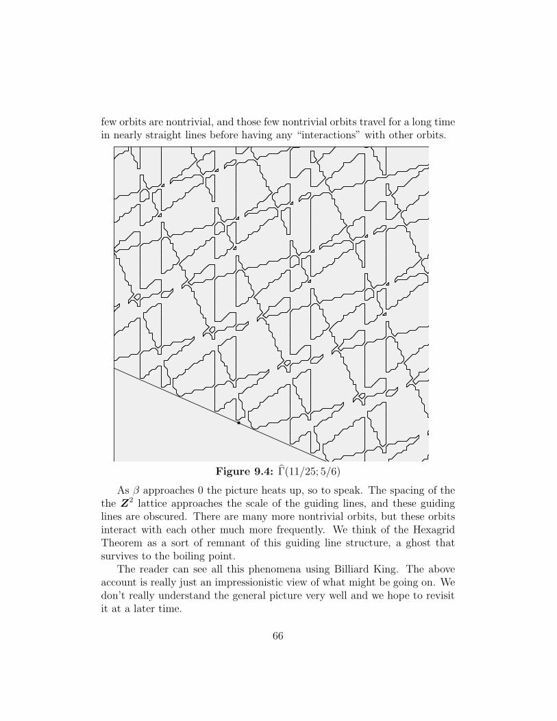
few orbits are nontrivial, and those few nontrivial orbits travel for a long timein nearly straight lines before having any “interactions” with other orbits.

Figure 9.4: Γ(11/25; 5/6)

As β approaches 0 the picture heats up, so to speak. The spacing of thethe Z2 lattice approaches the scale of the guiding lines, and these guidinglines are obscured. There are many more nontrivial orbits, but these orbitsinteract with each other much more frequently. We think of the HexagridTheorem as a sort of remnant of this guiding line structure, a ghost thatsurvives to the boiling point.

The reader can see all this phenomena using Billiard King. The aboveaccount is really just an impressionistic view of what might be going on. Wedon’t really understand the general picture very well and we hope to revisitit at a later time.

66

Part II:In this part of the monograph we will state and prove the Master Picture

Theorem. All the auxilliary theorems left over from Part I rely on this centralresult. Here is an overview of the material.

• In §10 we will state the Master Picture Theorem. Roughly, the MasterPicture Theorem says that the structure of the return map Ψ is de-termined by a pair of maps into a flat 3-torus, R3/Λ, together with apartition of R3/Λ into polyhedra. Here Λ is a certain 3-dimensionallattice that depends on the parameter.

• In §11, we will prove the Pinwheel Lemma, a key technical step alongthe way to our proof of the Master Picture Theorem. The PinwheelLemma states that we can factor the return map Ψ into a compositionof 8 simpler maps, which we call strip maps. A strip map is a verysimple map from the plane into an infinite strip.

• In §12 we prove the Torus Lemma, another key result. The TorusLemma implies that there exists some partition of our torus into openregions, such that the regions determine the structure of the arithmeticgraph. The Torus Lemma reduces the Master Picture Theorem to arough determination of the singular set. The singular set is the (closureof the) set of points in the torus corresponding to points where thereturn map is not defined.

• In §13 we verify, with the aid of symbolic manipulation, certain func-tional identities that arise in connection with the Torus Lemma. Thesefunction identities are the basis for our analysis of the singular set.

• In §14 we combine the Torus Lemma with the functional identities toprove the Master Picture Theorem.

• in §15 we will explain how one actually makes computations with theMaster Picture Theorem. §15.2 will be very important for Part IV ofthe monograph.

67

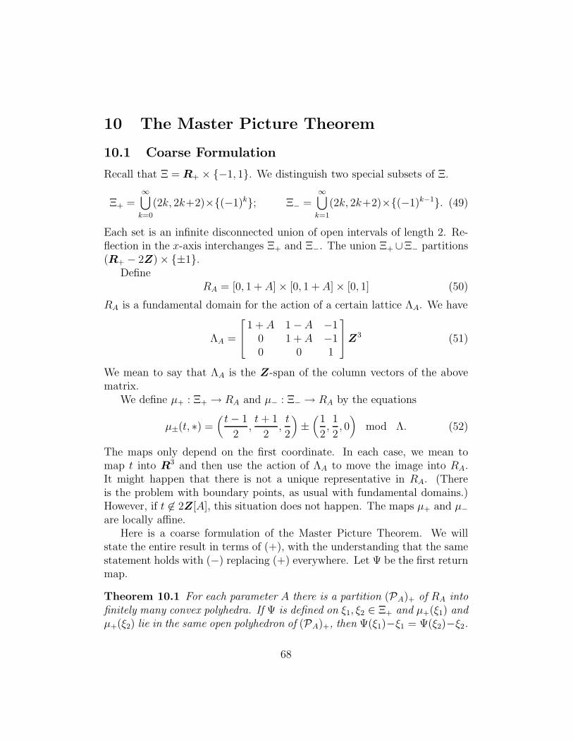
10 The Master Picture Theorem

10.1 Coarse Formulation

Recall that Ξ = R+ × {−1, 1}. We distinguish two special subsets of Ξ.

Ξ+ =∞⋃

k=0

(2k, 2k+2)×{(−1)k}; Ξ− =∞⋃

k=1

(2k, 2k+2)×{(−1)k−1}. (49)

Each set is an infinite disconnected union of open intervals of length 2. Re-flection in the x-axis interchanges Ξ+ and Ξ−. The union Ξ+ ∪Ξ− partitions(R+ − 2Z)× {±1}.

DefineRA = [0, 1 + A]× [0, 1 + A]× [0, 1] (50)

RA is a fundamental domain for the action of a certain lattice ΛA. We have

ΛA =

1 + A 1−A −10 1 + A −10 0 1

Z3 (51)

We mean to say that ΛA is the Z-span of the column vectors of the abovematrix.

We define µ+ : Ξ+ → RA and µ− : Ξ− → RA by the equations

µ±(t, ∗) =(t− 1

2,t+ 1

2,t

2

)±

(1

2,1

2, 0

)mod Λ. (52)

The maps only depend on the first coordinate. In each case, we mean tomap t into R3 and then use the action of ΛA to move the image into RA.It might happen that there is not a unique representative in RA. (Thereis the problem with boundary points, as usual with fundamental domains.)However, if t 6∈ 2Z[A], this situation does not happen. The maps µ+ and µ−

are locally affine.Here is a coarse formulation of the Master Picture Theorem. We will

state the entire result in terms of (+), with the understanding that the samestatement holds with (−) replacing (+) everywhere. Let Ψ be the first returnmap.

Theorem 10.1 For each parameter A there is a partition (PA)+ of RA intofinitely many convex polyhedra. If Ψ is defined on ξ1, ξ2 ∈ Ξ+ and µ+(ξ1) andµ+(ξ2) lie in the same open polyhedron of (PA)+, then Ψ(ξ1)−ξ1 = Ψ(ξ2)−ξ2.

68

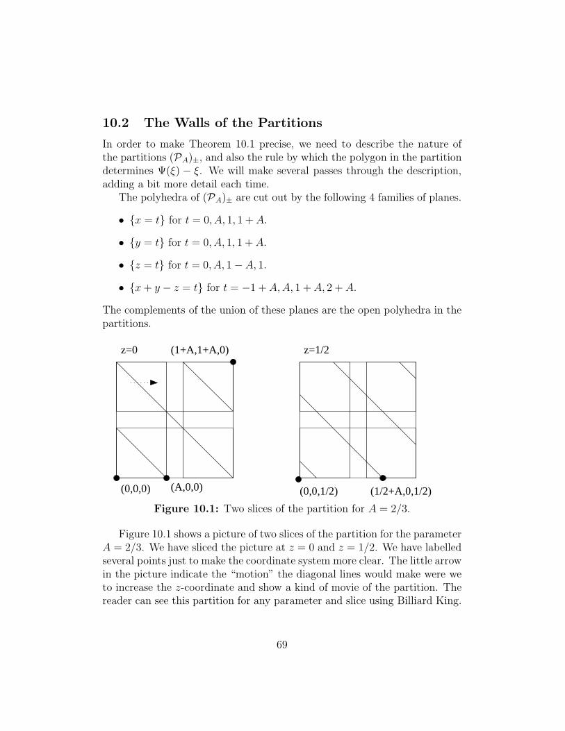
10.2 The Walls of the Partitions

In order to make Theorem 10.1 precise, we need to describe the nature ofthe partitions (PA)±, and also the rule by which the polygon in the partitiondetermines Ψ(ξ) − ξ. We will make several passes through the description,adding a bit more detail each time.

The polyhedra of (PA)± are cut out by the following 4 families of planes.

• {x = t} for t = 0, A, 1, 1 + A.

• {y = t} for t = 0, A, 1, 1 + A.

• {z = t} for t = 0, A, 1−A, 1.

• {x+ y − z = t} for t = −1 + A,A, 1 + A, 2 + A.

The complements of the union of these planes are the open polyhedra in thepartitions.

(1/2+A,0,1/2)(0,0,0) (A,0,0) (0,0,1/2)

z=0 z=1/2(1+A,1+A,0)

Figure 10.1: Two slices of the partition for A = 2/3.

Figure 10.1 shows a picture of two slices of the partition for the parameterA = 2/3. We have sliced the picture at z = 0 and z = 1/2. We have labelledseveral points just to make the coordinate system more clear. The little arrowin the picture indicate the “motion” the diagonal lines would make were weto increase the z-coordinate and show a kind of movie of the partition. Thereader can see this partition for any parameter and slice using Billiard King.

69

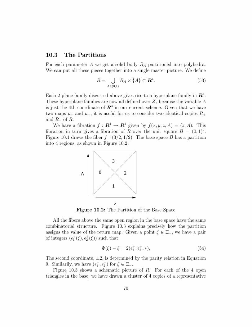
10.3 The Partitions

For each parameter A we get a solid body RA partitioned into polyhedra.We can put all these pieces together into a single master picture. We define

R =⋃

A∈(0,1)

RA × {A} ⊂ R4. (53)

Each 2-plane family discussed above gives rise to a hyperplane family in R4.These hyperplane families are now all defined over Z, because the variable Ais just the 4th coordinate of R4 in our current scheme. Given that we havetwo maps µ+ and µ−, it is useful for us to consider two identical copies R+

and R− of R.We have a fibration f : R4 → R2 given by f(x, y, z, A) = (z, A). This

fibration in turn gives a fibration of R over the unit square B = (0, 1)2.Figure 10.1 draws the fiber f−1(3/2, 1/2). The base space B has a partitioninto 4 regions, as shown in Figure 10.2.

z

2

3

0

1

A

Figure 10.2: The Partition of the Base Space

All the fibers above the same open region in the base space have the samecombinatorial structure. Figure 10.3 explains precisely how the partitionassigns the value of the return map. Given a point ξ ∈ Ξ+, we have a pairof integers (ǫ+1 (ξ), ǫ+2 (ξ)) such that

Ψ(ξ)− ξ = 2(ǫ+1 , ǫ+2 , ∗). (54)

The second coordinate, ±2, is determined by the parity relation in Equation9. Similarily, we have (ǫ−1 , ǫ

−

2 ) for ξ ∈ Ξ−.Figure 10.3 shows a schematic picture of R. For each of the 4 open

triangles in the base, we have drawn a cluster of 4 copies of a representative

70

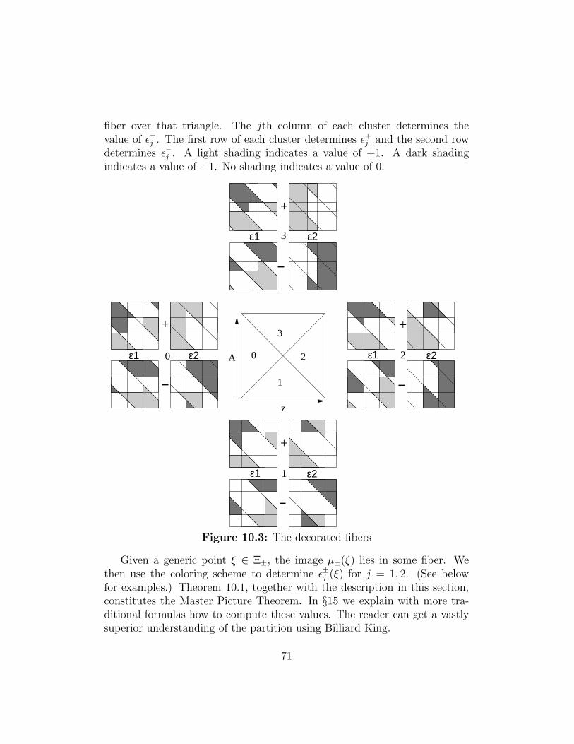
fiber over that triangle. The jth column of each cluster determines thevalue of ǫ±j . The first row of each cluster determines ǫ+j and the second rowdetermines ǫ−j . A light shading indicates a value of +1. A dark shadingindicates a value of −1. No shading indicates a value of 0.

2

3

0

1

z

A 20

3

1

+

ε1 ε2

ε1 ε2

ε2ε1

ε2ε1

+ +

+

Figure 10.3: The decorated fibers

Given a generic point ξ ∈ Ξ±, the image µ±(ξ) lies in some fiber. Wethen use the coloring scheme to determine ǫ±j (ξ) for j = 1, 2. (See belowfor examples.) Theorem 10.1, together with the description in this section,constitutes the Master Picture Theorem. In §15 we explain with more tra-ditional formulas how to compute these values. The reader can get a vastlysuperior understanding of the partition using Billiard King.

71

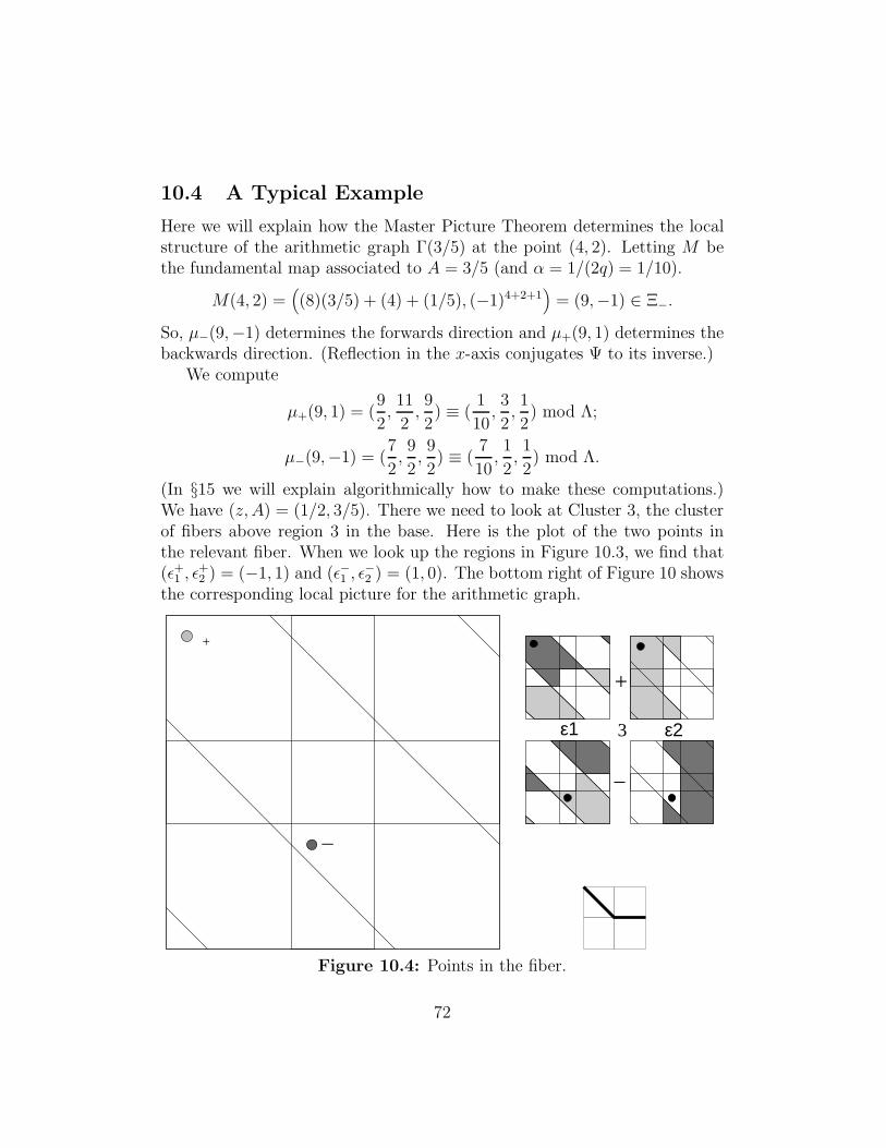
10.4 A Typical Example

Here we will explain how the Master Picture Theorem determines the localstructure of the arithmetic graph Γ(3/5) at the point (4, 2). Letting M bethe fundamental map associated to A = 3/5 (and α = 1/(2q) = 1/10).

M(4, 2) =((8)(3/5) + (4) + (1/5), (−1)4+2+1

)= (9,−1) ∈ Ξ−.

So, µ−(9,−1) determines the forwards direction and µ+(9, 1) determines thebackwards direction. (Reflection in the x-axis conjugates Ψ to its inverse.)

We compute

µ+(9, 1) = (9

2,11

2,9

2) ≡ (

1

10,3

2,1

2) mod Λ;

µ−(9,−1) = (7

2,9

2,9

2) ≡ (

7

10,1

2,1

2) mod Λ.

(In §15 we will explain algorithmically how to make these computations.)We have (z, A) = (1/2, 3/5). There we need to look at Cluster 3, the clusterof fibers above region 3 in the base. Here is the plot of the two points inthe relevant fiber. When we look up the regions in Figure 10.3, we find that(ǫ+1 , ǫ

+2 ) = (−1, 1) and (ǫ−1 , ǫ

−

2 ) = (1, 0). The bottom right of Figure 10 showsthe corresponding local picture for the arithmetic graph.

3

+

+

ε1 ε2

Figure 10.4: Points in the fiber.

72

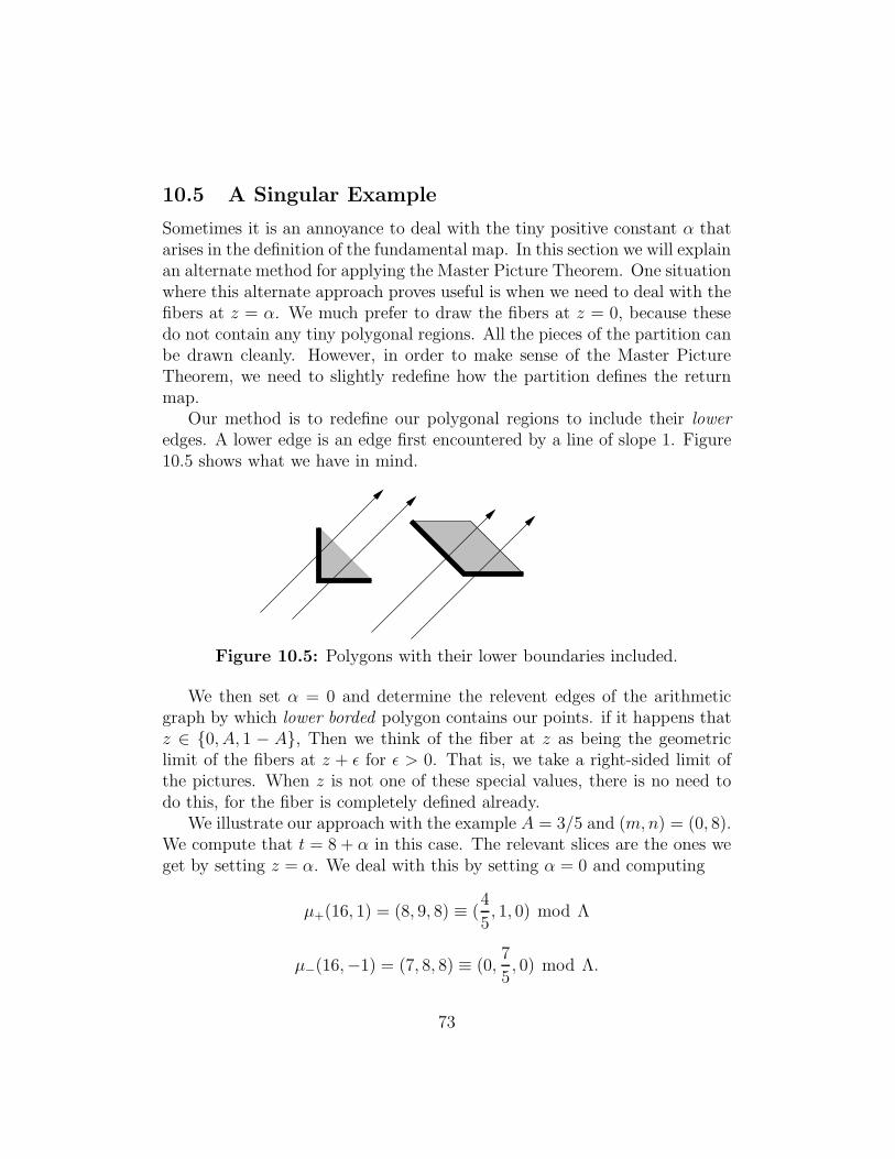
10.5 A Singular Example

Sometimes it is an annoyance to deal with the tiny positive constant α thatarises in the definition of the fundamental map. In this section we will explainan alternate method for applying the Master Picture Theorem. One situationwhere this alternate approach proves useful is when we need to deal with thefibers at z = α. We much prefer to draw the fibers at z = 0, because thesedo not contain any tiny polygonal regions. All the pieces of the partition canbe drawn cleanly. However, in order to make sense of the Master PictureTheorem, we need to slightly redefine how the partition defines the returnmap.

Our method is to redefine our polygonal regions to include their loweredges. A lower edge is an edge first encountered by a line of slope 1. Figure10.5 shows what we have in mind.

Figure 10.5: Polygons with their lower boundaries included.

We then set α = 0 and determine the relevent edges of the arithmeticgraph by which lower borded polygon contains our points. if it happens thatz ∈ {0, A, 1 − A}, Then we think of the fiber at z as being the geometriclimit of the fibers at z + ǫ for ǫ > 0. That is, we take a right-sided limit ofthe pictures. When z is not one of these special values, there is no need todo this, for the fiber is completely defined already.

We illustrate our approach with the example A = 3/5 and (m,n) = (0, 8).We compute that t = 8 + α in this case. The relevant slices are the ones weget by setting z = α. We deal with this by setting α = 0 and computing

µ+(16, 1) = (8, 9, 8) ≡ (4

5, 1, 0) mod Λ

µ−(16,−1) = (7, 8, 8) ≡ (0,7

5, 0) mod Λ.

73

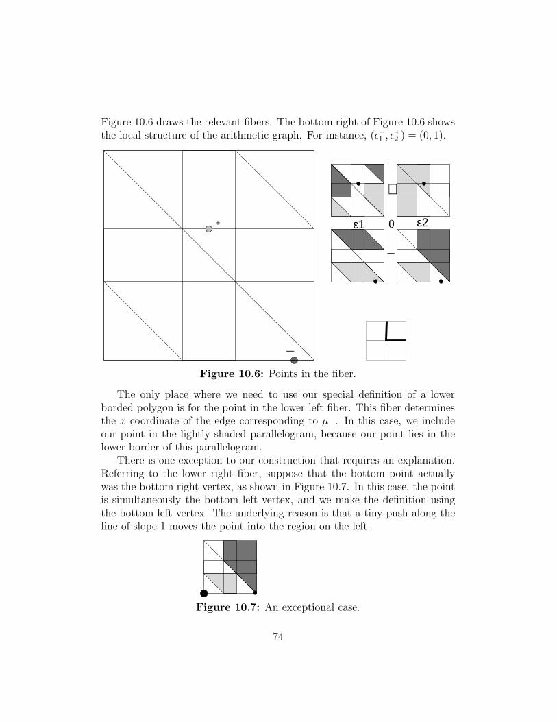
Figure 10.6 draws the relevant fibers. The bottom right of Figure 10.6 showsthe local structure of the arithmetic graph. For instance, (ǫ+1 , ǫ

+2 ) = (0, 1).

+ 0ε1 ε2

+

−

Figure 10.6: Points in the fiber.

The only place where we need to use our special definition of a lowerborded polygon is for the point in the lower left fiber. This fiber determinesthe x coordinate of the edge corresponding to µ−. In this case, we includeour point in the lightly shaded parallelogram, because our point lies in thelower border of this parallelogram.

There is one exception to our construction that requires an explanation.Referring to the lower right fiber, suppose that the bottom point actuallywas the bottom right vertex, as shown in Figure 10.7. In this case, the pointis simultaneously the bottom left vertex, and we make the definition usingthe bottom left vertex. The underlying reason is that a tiny push along theline of slope 1 moves the point into the region on the left.

Figure 10.7: An exceptional case.

74

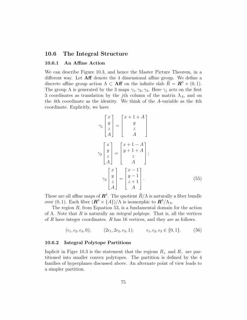
10.6 The Integral Structure

10.6.1 An Affine Action

We can describe Figure 10.3, and hence the Master Picture Theorem, in adifferent way. Let Aff denote the 4 dimensional affine group. We define adiscrete affine group action Λ ⊂ Aff on the infinite slab R = R3 × (0, 1).The group Λ is generated by the 3 maps γ1, γ2, γ3. Here γj acts on the first3 coordinates as translation by the jth column of the matrix ΛA, and onthe 4th coordinate as the identity. We think of the A-variable as the 4thcoordinate. Explicitly, we have

γ1

xyzA

=

x+ 1 + AyzA

γ2

xyzA

=

x+ 1− Ay + 1 + A

zA

;

γ3

xyzA

=

x− 1y − 1z + 1A

. (55)

These are all affine maps of R4. The quotient R/Λ is naturally a fiber bundleover (0, 1). Each fiber (R3 × {A})/Λ is isomorphic to R3/ΛA.

The region R, from Equation 53, is a fundamental domain for the actionof Λ. Note that R is naturally an integral polytope. That is, all the verticesof R have integer coordinates. R has 16 vertices, and they are as follows.

(ǫ1, ǫ2, ǫ3, 0); (2ǫ1, 2ǫ2, ǫ3, 1); ǫ1, ǫ2, ǫ3 ∈ {0, 1}. (56)

10.6.2 Integral Polytope Partitions

Inplicit in Figre 10.3 is the statement that the regions R+ and R− are par-titioned into smaller convex polytopes. The partition is defined by the 4families of hyperplanes discussed above. An alternate point of view leads toa simpler partition.

75

For each pair (ǫ1, ǫ2) ∈ {−1, 0, 1}, we let R+(ǫ1, ǫ2) denote the closure ofthe union of regions that assign (ǫ1, ǫ2). It turns out that R(ǫ1, ǫ2) if a finiteunion of convex integral polytopes. There are 14 such polytopes, and theygive an integral partition of R+. We list these polytopes in §15.4.

Let ι : R+ → R− be given by the map

ι(x, y, z, A) = (1 + A− x, 1 + A− y, 1− z, A). (57)

Geometrically, ι is a reflection in the 1-dimensional line. We have the generalequation

R−(−ǫ1,−ǫ2) = ι(R+(ǫ1, ǫ2)). (58)

Thus, the partition of R− is a mirror image of the partition of R+. (SeeExample 15.5 for an example calculation.)

We use the action of Λ to extend the partitions of R+ and R− to twointegral polytope tilings of R. (Again, see §15.5 for an example calculation.)These 4 dimensional tilings determine the structure of the special orbits.

10.6.3 Notation

Suppose that Γ is an arithmetic graph. Let M be the fundamental mapassociated to Γ. We define

M+ = µ+ ◦M ; M− = µ− ◦ ρ ◦M. (59)

Here ρ is reflection in the x-axis. Given a point p ∈ Z2, the polytope ofR+ containing M+(p) determines the forward edge of Γ incident to p, andthe polytope of R− containing M−(p) determines the backward edge of Γincident to p. Concretely, we have

M+(m,n) = (s, s+ 1, s) modΛ;

M−(m,n) = (s− 1, s, s) modΛ;

s = Am+ n+ α. (60)

As usual, α is the offset value. Note that µ+ and µ− only depend on thefirst coordinate, and this first coordinate is not changed by ρ. The map ρis present mainly for bookkeeping purposes, because ρ(Ξ+) = Ξ−, and thedomain of µ± is Ξ±.

76

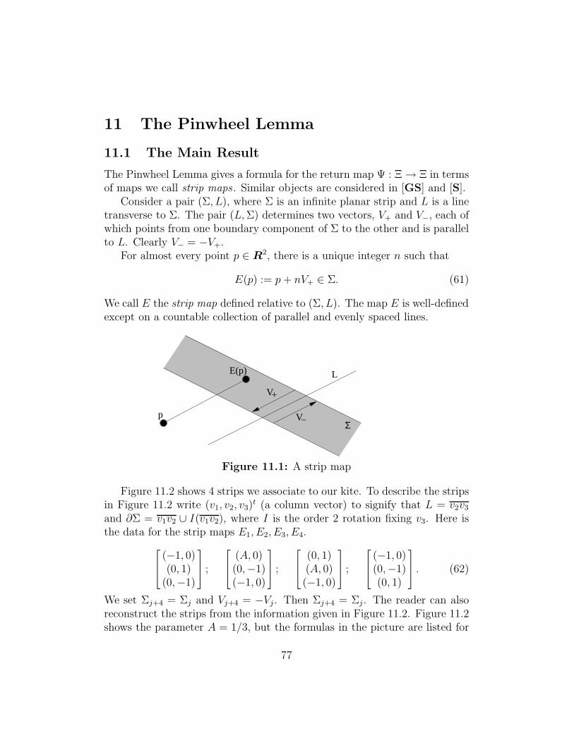
11 The Pinwheel Lemma

11.1 The Main Result

The Pinwheel Lemma gives a formula for the return map Ψ : Ξ→ Ξ in termsof maps we call strip maps. Similar objects are considered in [GS] and [S].

Consider a pair (Σ, L), where Σ is an infinite planar strip and L is a linetransverse to Σ. The pair (L,Σ) determines two vectors, V+ and V−, each ofwhich points from one boundary component of Σ to the other and is parallelto L. Clearly V− = −V+.

For almost every point p ∈ R2, there is a unique integer n such that

E(p) := p+ nV+ ∈ Σ. (61)

We call E the strip map defined relative to (Σ, L). The map E is well-definedexcept on a countable collection of parallel and evenly spaced lines.

p

L

Σ

E(p)

V

+V

−

Figure 11.1: A strip map

Figure 11.2 shows 4 strips we associate to our kite. To describe the stripsin Figure 11.2 write (v1, v2, v3)

t (a column vector) to signify that L = v2v3

and ∂Σ = v1v2 ∪ I(v1v2), where I is the order 2 rotation fixing v3. Here isthe data for the strip maps E1, E2, E3, E4.

(−1, 0)(0, 1)

(0,−1)

;

(A, 0)(0,−1)(−1, 0)

;

(0, 1)(A, 0)(−1, 0)

;

(−1, 0)(0,−1)(0, 1)

. (62)

We set Σj+4 = Σj and Vj+4 = −Vj . Then Σj+4 = Σj . The reader can alsoreconstruct the strips from the information given in Figure 11.2. Figure 11.2shows the parameter A = 1/3, but the formulas in the picture are listed for

77

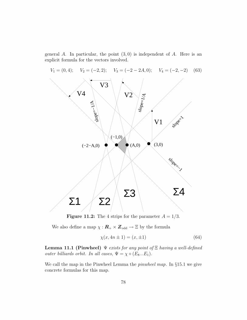
general A. In particular, the point (3, 0) is independent of A. Here is anexplicit formula for the vectors involved.

V1 = (0, 4); V2 = (−2, 2); V3 = (−2− 2A, 0); V4 = (−2,−2) (63)

Σ1

V1

V4 V2

V3

Σ4Σ3Σ2

(−2−A,0)

slope

=1

slope=−1

slop

e=1/

A

slop

e=−

1/A

(A,0) (3,0)

(−1,0)

Figure 11.2: The 4 strips for the parameter A = 1/3.

We also define a map χ : R+ ×Zodd → Ξ by the formula

χ(x, 4n± 1) = (x,±1) (64)

Lemma 11.1 (Pinwheel) Ψ exists for any point of Ξ having a well-definedouter billiards orbit. In all cases, Ψ = χ ◦ (E8...E1).

We call the map in the Pinwheel Lemma the pinwheel map. In §15.1 we giveconcrete formulas for this map.

78

11.2 Some Corollaries

Before we prove the Pinwheel Lemma, we list two corollaries.

Corollary 11.2 The parity equation in Equation 9 is true.

Proof: The Pinwheel Lemma tells us that

Ψ(x, 1)− (x, 1) = 2(ǫ1A+ ǫ2, ǫ3); (ǫ1, ǫ2, ǫ3) ∈ Z2 × {−1, 0, 1}. (65)

Given Equation 63, we see that the sum of the integer coefficients in eachvector Vj is divisible by 4. (For instance, −2 − 2A yields −2 − 2 = −4.)Hence ǫ1 + ǫ2 + ǫ3 is even. ♠

The Pinwheel Lemma gives a formula for the quantities in Equation 9.For j = 0, ..., 7 we define points pj+1 and integers nj by the following

equations.pj+1 = Ej+1(pj) = pj + njVj+1. (66)

Given the equations

V1 = (0, 4); V2 = (−2, 2); V3 = (−2− 2A, 0); V4 = (−2,−2) (67)

we find that

ǫ1 = n2 − n6; ǫ2 = n1 + n2 + n3 − n5 − n6 − n7; (68)

We call (n1, ..., n7) the length spectrum of p0.The precise bound in Equation 9 follows from the Master Picture Theo-

rem, but here we give a heuristic explanation. If we define

m1 = n7; m2 = n6; m3 = n5; (69)

then we have

ǫ1(p) = n2 −m2; ǫ2(p) = (n1 −m1) + (n2 −m2) + (n3 −m3). (70)

The path with vertices p0, p1, ..., p7, p8, χ(p8) uniformly close to an octagonwith dihedral symmetry. See Figure 11.3 below. For this reason, there is auniversal bound to |ni−mi|. This is a heuristic explanation of the bound inEquation 9.

79

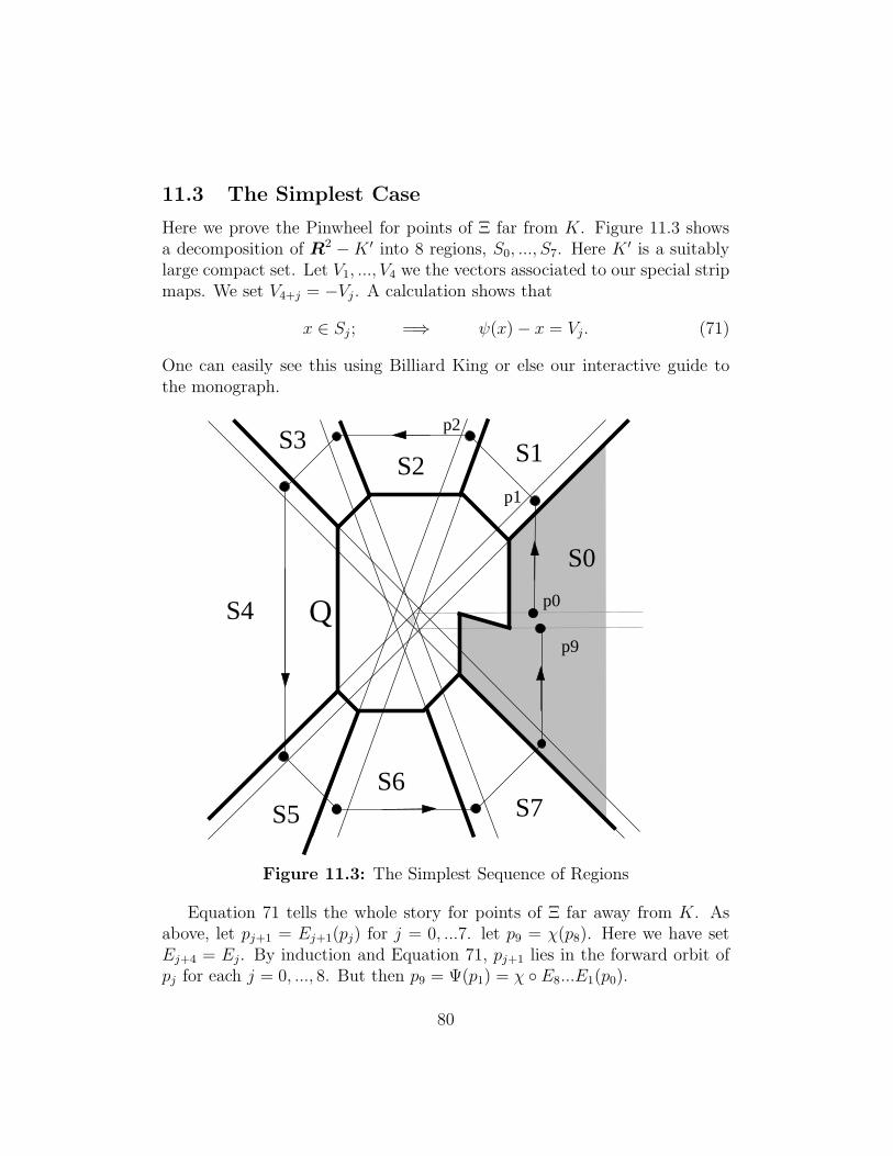
11.3 The Simplest Case

Here we prove the Pinwheel for points of Ξ far from K. Figure 11.3 showsa decomposition of R2 −K ′ into 8 regions, S0, ..., S7. Here K ′ is a suitablylarge compact set. Let V1, ..., V4 we the vectors associated to our special stripmaps. We set V4+j = −Vj . A calculation shows that

x ∈ Sj ; =⇒ ψ(x)− x = Vj. (71)

One can easily see this using Billiard King or else our interactive guide tothe monograph.

S4

S5

S3

S7

S1

S0

S6

Q p0

p1

p2

p9

S2

Figure 11.3: The Simplest Sequence of Regions

Equation 71 tells the whole story for points of Ξ far away from K. Asabove, let pj+1 = Ej+1(pj) for j = 0, ...7. let p9 = χ(p8). Here we have setEj+4 = Ej. By induction and Equation 71, pj+1 lies in the forward orbit ofpj for each j = 0, ..., 8. But then p9 = Ψ(p1) = χ ◦ E8...E1(p0).

80

11.4 Discussion of the General Case

As we have just seen, the Pinwheel Lemma is a fairly trivial result for pointsthat are far from the origin. For points near the origin, the Pinwheel Lemmais a surprising and nontrivial result. In fact, it only seems to work becauseof a lucky accident. The fact that we consider the Pinwheel Lemma to bean accident probably means that we don’t yet have a good understanding ofwhat is going on.

Verifying the Pinwheel Lemma for any given parameter A is a finite calcu-lation. We just have to check, on a fine enough mesh of points extending outsufficiently far away from K(A), that the equation in the Pinwheel Lemmaholds. The point is that all the maps involved are piecewise isometries foreach parameter. We took this approach in [S] when we proved the PinwheelLemma for A = φ−3.

Using Billiard King, we computed that the Pinwheel Lemma holds trueat the points (x,±1) relative to the parameter A for all

A =1

256, ...,

255

256; x = ǫ+

1

1024, ..., ǫ+

16384

1024; ǫ = 10−6.

The tiny number ǫ is included to make sure that the outer billiards orbitis actually defined for all the points we sample. This calculation does notconstitute a proof of anything. However, we think that it serves as a pow-erful sanity check that the Pinwheel Lemma is correct. We have fairly wellcarpeted the region of doubt about the Pinwheel Lemma with instances ofits truth.

Our proof of the Pinwheel Lemma essentially boils down to finding thereplacement equation for Equation 71. We will do this in the section. As thereader will see, the situation in general is much more complicated. There isa lot of information packed into the next section, but all this information iseasily seen visually on Billiard King. We have programmed Billiard King sothat the reader can see pictures of all the regions involved, as well as theirinteractions, for essentially any desired parameter.

We think of the material in the next section as something like a writtendescription of a photograph. The written word is probably not the rightmedium for the proof of the Pinwheel Lemma. To put this in a different way,Billiard King relates to the proof given here much in the same way that anordinary research paper would relate to one that was written in crayon.

81

11.5 A Partition of the Plane

Let ψ = ψA be the square of the outer billiards map relative to K(A). Foreach x ∈ R2 −K on which ψ is defined, there is a vector vx such that

ψ(x)− x = vx.

This vector is twice the difference between 2 vertices of K, and therefore cantake on 12 possible values. It turns out that 10 of these values occur. Wecall these vectors Vj , with j = 1, 2, 3, 4, 4♯, 5, 6♭, 6, 7, 8. With this ordering,the argument of Vj increases monotonically with j. Compare Figure 11.4.For each of our vectors V , there is an open region R ⊂ R2 − K such thatx ∈ R if and only if ψ(x) − x = V . The regions R1, ..., R8 are unbounded.The two regions R♯

4 and R♭6 are bounded.

One can find the entire partition by extending the sides of K in onedirection, in a pinwheel fashion, and then pulling back these rays by the outerbilliards map. To describe the regions, we use the notation −→q1 , p1, ..., pk,

−→q2to indicate that

• The two unbounded edges are {p1 + tq1| t ≥ 0} and {pk + tq2| t ≥ 0}.

• p2, ..., pk−1 are any additional intermediate vertices.

To improve the typesetting on our list, we set λ = (A − 1)−1. Figure 10.3shows the picture for A = 1/3. The reader can see any parameter usingBilliard King.

V1 =(0, 4). R1 :−−−−→(1,−1), (1,−2),

−−−→(1, 1).

V2 =(−2, 2). R2 :−−−→(1, 1), (1,−2), (0,−1),

−−−→(A, 1).

V3 =(−2−2A, 0) R3 :−−−→(A, 1), (2A, 1), λ(2A2,−1− A),

−−−−→(−A, 1).

V4 =(−2,−2) R4 :−−−−→(−A, 1), λ(2A,A− 3),

−−−−→(−1, 1).

V4♯ =(−2A,−2) R4♯ : (A, 0), (2A, 1), λ(2A2,−1−A))

V5 =(0,−4) R5 :−−−−→(−1, 1), λ(2A,A−3), (−A, 2), λ(2A, 3A−1),

−−−−−→(−1,−1)

V6♭ =(2A,−2) R6♭ : (0, 1), (−A, 2), λ(2A, 3A− 1)

V6 =(2,−2) R6 :−−−−−→(−1,−1), λ(2, A+ 1),

−−−−−−→(−A,−1)

V7 =(2 + 2A, 0) R7 :−−−−−−→(−A,−1), λ(2, A+ 1), (−2,−1),

−−−−→(A,−1)

V8 =(2, 2) R8 :−−−−→(A,−1), (−2,−1), (−1, 0),

−−−−→(1,−1).

82

#

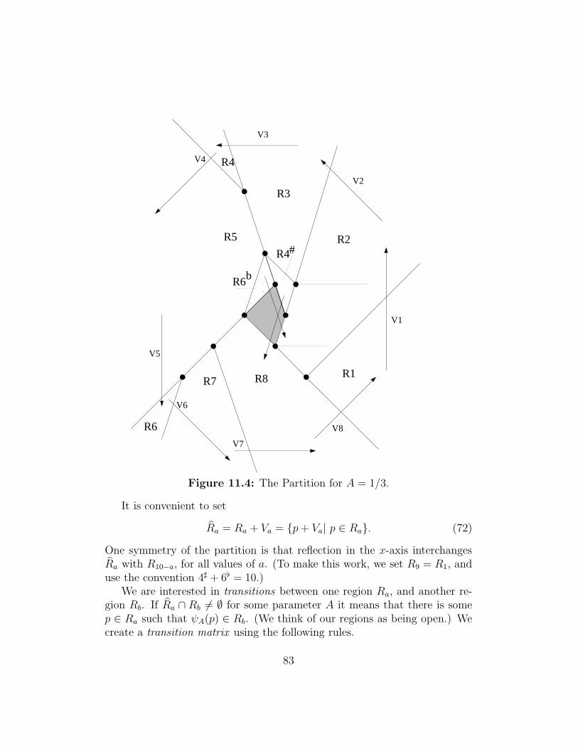
V1

V2

V3

V4

V5

V6

V7

V8

R6b

R4

R1R8R7

R5

R6

R2

R4

R3

Figure 11.4: The Partition for A = 1/3.

It is convenient to set

Ra = Ra + Va = {p+ Va| p ∈ Ra}. (72)

One symmetry of the partition is that reflection in the x-axis interchangesRa with R10−a, for all values of a. (To make this work, we set R9 = R1, anduse the convention 4♯ + 6♭ = 10.)

We are interested in transitions between one region Ra, and another re-gion Rb. If Ra ∩ Rb 6= ∅ for some parameter A it means that there is somep ∈ Ra such that ψA(p) ∈ Rb. (We think of our regions as being open.) Wecreate a transition matrix using the following rules.

83

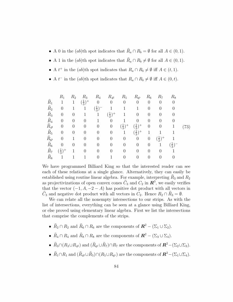
• A 0 in the (ab)th spot indicates that Ra ∩Rb = ∅ for all A ∈ (0, 1).

• A 1 in the (ab)th spot indicates that Ra ∩Rb 6= ∅ for all A ∈ (0, 1).

• A t+ in the (ab)th spot indicates that Ra ∩ Rb 6= ∅ iff A ∈ (t, 1).

• A t− in the (ab)th spot indicates that Ra ∩ Rb 6= ∅ iff A ∈ (0, t).

R1 R2 R3 R4 R4♯ R5 R6♭ R6 R7 R8

R1 1 1 (13)+ 0 0 0 0 0 0 0

R2 0 1 1 (13)− 1 1 1 0 0 0

R3 0 0 1 1 (12)+ 1 0 0 0 0

R4 0 0 0 1 0 1 0 0 0 0R4♯ 0 0 0 0 0 (1

3)+ (1

3)+ 0 0 1

R5 0 0 0 0 0 1 (13)+ 1 1 1

R6♭ 0 1 0 0 0 0 0 0 (12)+ 1

R6 0 0 0 0 0 0 0 0 1 (13)−

R7 (13)+ 1 0 0 0 0 0 0 0 1

R8 1 1 1 0 1 0 0 0 0 0

(73)

We have programmed Billiard King so that the interested reader can seeeach of these relations at a single glance. Alternatively, they can easily beestablished using routine linear algebra. For example, interpreting R3 and R2

as projectivizations of open convex cones C3 and C2 in R3, we easily verifiesthat the vector (−1, A,−2− A) has positive dot product with all vectors inC3 and negative dot product with all vectors in C2. Hence R2 ∩ R3 = ∅.

We can relate all the nonempty intersections to our strips. As with thelist of intersections, everything can be seen at a glance using Billiard King,or else proved using elementary linear algebra. First we list the intersectionsthat comprise the complements of the strips.

• R2 ∩ R2 and R6 ∩R6 are the components of R2 − (Σ1 ∪ Σ2).

• R4 ∩ R4 and R8 ∩R8 are the components of R2 − (Σ3 ∪ Σ4).

• R3∩(R3∪R4♯) and (R6♭∪R7)∩R7 are the components of R2−(Σ2∪Σ3).

• R1∩R1 and (R4♯∪R5)∩(R5∪R6♭) are the components of R2−(Σ1∪Σ4).

84

Now we list the intersections that are contained in single strips. To makeour typesetting nicer, we use the term u-component to denote an unboundedconnected component. We use the term b-component to denote a boundedconnected component.

• R1 ∩ R2 and R5 ∩R6 are the two u-components of Σ1 − (Σ2 ∪ Σ4).

• R8 ∩ R1 and R4 ∩R5 are the two u-components of Σ4 − (Σ1 ∪ Σ3).

• R3∩R4 and (R6♭∪R7)∩R8 are the two u-components of Σ3−(Σ2∪Σ4).

• R6∩R7 and R2∩(R3∪R4♯) are the two u-components of Σ2−(Σ1∪Σ3).

• R6♭ ∩ R7 is contained in the b-component of Σ1 − (Σ2 ∪ Σ3).

• R3 ∩ R4♯ is contained in the b-component of Σ4 − (Σ2 ∪ Σ3).

• R4♯ ∩ (R5 ∪ R6♭) is contained in the b-component of Σ3 − (Σ1 ∪ Σ4).

• (R4♯ ∪ R5) ∩ R6♭ is contained in the b-component of Σ2 − (Σ1 ∪ Σ4).

Now we list the intersections of regions that are contained in doubleintersections of strips. In this case, all the components are bounded: Anytwo strips intersect in a bounded region of the plane.

• R1 ∩ R3 and R5 ∩R7 are the components of (Σ1 ∩ Σ2)− (Σ3 ∪ Σ4).

• R7 ∩ R1 and R3 ∩R5 are the components of (Σ3 ∩ Σ4)− (Σ1 ∪ Σ2).

• R2∩R4 and R6∩R8 are bounded components of (Σ2∩Σ3)− (Σ1∪Σ4).

• R8 ∩ R2 = (Σ1 ∩ Σ4)− (Σ2 ∪ Σ3).

Now we list all the intersections of regions that are contained in tripleintersections of strips.

• R2 ∩ (R5 ∪R6♭) = Σ2 ∩ Σ3 ∩ Σ4 − Σ1.

• R8 ∩ (R3 ∪R4♯) = Σ1 ∩ Σ2 ∩ Σ4 − Σ3.

• (R4♯ ∪ R5) ∩ R8 = Σ1 ∩ Σ2 ∩ Σ3 − Σ4.

• (R6♭ ∪ R7) ∩ R2 = Σ1 ∩ Σ3 ∩ Σ4 − Σ2.

85

Here we list a bit more information about the two regions R4♯ and R6♭

some of the information is redundant, but it is useful to have it all in oneplace.

• R4♯ ⊂ Σ4 − Σ3.

• R4♯ + V3 = Σ3 − (Σ2 ∪ Σ4).

• R6♭ ⊂ Σ2 − Σ1.

• R6♭ + V5 ⊂ Σ1 − Σ2.

• R6♭ + V5 − V6 = Σ2 − (Σ1 ∪ Σ3).

Finally, we mention two crucial relations between our various vectors:

• V3 − V4 + V5 = V4♯ .

• V5 − V6 + V7 = V6♭ .

These two relations are responsible for the lucky cancellation that makes thePinwheel Lemma hold near the kite.

We will change our notation slightly from the simplest case consideredabove. Given any point z1 ∈ Ξ, we can associate the sequence of regions

Ra1→ ...→ Rak

(74)

through which the forwards orbit of z1 transitions until it returns as Ψ(z1).The simplest possible sequence is the one where aj = j for j = 1, ..., 9. SeeFigure 11.2. We already analyzed this case in §11.2. We let zj denote thefirst point in the forward orbit of z1 that lies in Raj

.To prove the Pinwheel Lemma in general, we need to analyze all allowable

sequences and see that the equation in the Pinwheel Lemma always holds.We will break the set of all sequences into three types, and then analyze thetypes one at a time. Here are the types.

1. Sequences that do not involve the indices 4♯ or 6♭.

2. Sequences that involve 4♯ but not 6♭.

3. Sequences that involve 6♭.

86

11.6 No Sharps or Flats

Lemma 11.3 If j < k then Rj ∩ Rk ⊂ Σj ∩ ... ∩ Σk−1.

Proof: This is a corollary of the the intersections listed above. ♠

Suppose by induction we have shown that

zj = Eaj−1Eaj−2...E1(z1). (75)

By construction and Lemma 11.3,

zj+1 = Eaj(zj) ∈ Raj

∩ Raj+1⊂ Σaj

∩ ... ∩ Σaj+1−1.

Therefore, Eaj, ..., Eaj+1−1 all act trivially on zj+1, forcing

zj+1 = Eaj+1−1Eaj+1−2...E1(z1).

Hence, Equation 75 holds true for all indices j.By the Intersection Lemma, we eventually reach either a point z9 or z10.

(That is, we wrap all the way around and return either to R9 = R1 or elseto R10 = R2.) We will consider these two cases one at a time.

Case 1: If we reach z9 = (x9, y9) ∈ R9 then we have

z9 = E8...E1(z1); x9 > 0; y9 ≤ 1. (76)

From this we get that Ψ(z1) = χ ◦ (E4...E1)2(z1), as desired. The last in-

equality in Equation 76 requires explanation. By the Intersection Lemma,the point preceding z9 on our list must lie in Ra for some a ∈ {6♭, 6, 7, 8}.However, the distance between any point on R+×{3, 5, 7...} to any point inRa exceeds the length of vector Va.

Case 2: If we arrive at z10 = (x10, y10), then the Intersection Lemma tellsus that the point preceding z10 lies in Va for a = {6♭, 6, 7, 8} and z10 ∈ Σ9.Hence E9(z10) = z10. That is

z10 = E8...E1(z1); x10 > 0; y10 < 3.

The last inequality works just as in Case 1. All points in R10 have y-coordinate at least −2. Hence y10 = ±1. Hence χ(z10) = z10. Puttingeverything together gives the same result as Case 1.

87

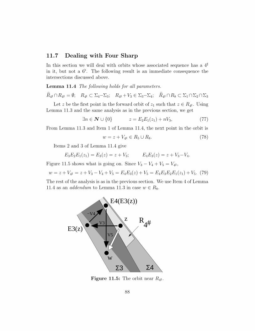
11.7 Dealing with Four Sharp

In this section we will deal with orbits whose associated sequence has a 4♯

in it, but not a 6♭. The following result is an immediate consequence theintersections discussed above.

Lemma 11.4 The following holds for all parameters.

R4♯ ∩R4♯ = ∅; R4♯ ⊂ Σ4−Σ3; R4♯ +V3 ∈ Σ3−Σ4; R4♯ ∩R8 ⊂ Σ1∩Σ2∩Σ3

Let z be the first point in the forward orbit of z1 such that z ∈ R4♯ . UsingLemma 11.3 and the same analysis as in the previous section, we get

∃n ∈N ∪ {0} z = E2E1(z1) + nV3, (77)

From Lemma 11.3 and Item 1 of Lemma 11.4, the next point in the orbit is

w = z + V4♯ ∈ R5 ∪R8. (78)

Items 2 and 3 of Lemma 11.4 give

E3E2E1(z1) = E3(z) = z + V3; E4E3(z) = z + V3−V4.

Figure 11.5 shows what is going on. Since V3 − V4 + V5 = V4♯ ,

w = z+ V4♯ = z+ V3− V4 + V5 = E4E3(z) + V5 = E4E3E2E1(z1) + V5. (79)

The rest of the analysis is as in the previous section. We use Item 4 of Lemma11.4 as an addendum to Lemma 11.3 in case w ∈ R8.

4#Rz

w

E3(z)

E4(E3(z))

Σ3 Σ4

−V4

V3

V5

Figure 11.5: The orbit near R4♯ .

88

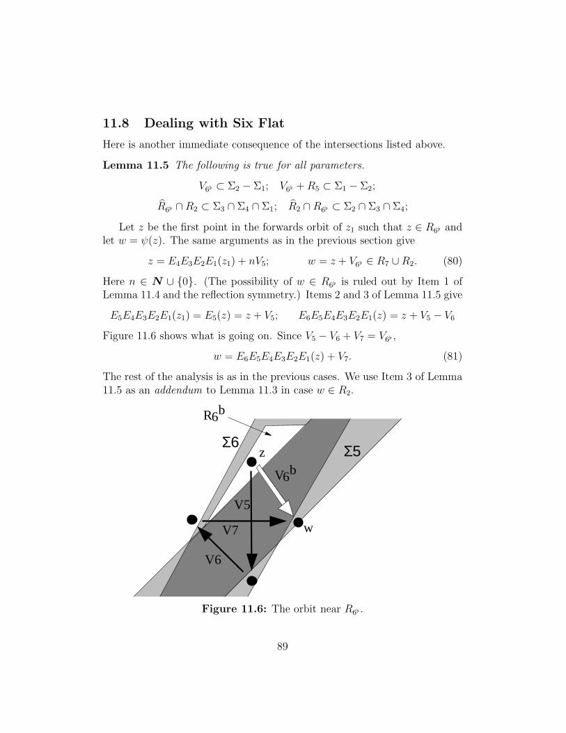
11.8 Dealing with Six Flat

Here is another immediate consequence of the intersections listed above.

Lemma 11.5 The following is true for all parameters.

V6♭ ⊂ Σ2 − Σ1; V6♭ +R5 ⊂ Σ1 − Σ2;

R6♭ ∩R2 ⊂ Σ3 ∩ Σ4 ∩ Σ1; R2 ∩ R6♭ ⊂ Σ2 ∩ Σ3 ∩ Σ4;

Let z be the first point in the forwards orbit of z1 such that z ∈ R6♭ andlet w = ψ(z). The same arguments as in the previous section give

z = E4E3E2E1(z1) + nV5; w = z + V6♭ ∈ R7 ∪R2. (80)

Here n ∈ N ∪ {0}. (The possibility of w ∈ R6♭ is ruled out by Item 1 ofLemma 11.4 and the reflection symmetry.) Items 2 and 3 of Lemma 11.5 give

E5E4E3E2E1(z1) = E5(z) = z + V5; E6E5E4E3E2E1(z) = z + V5 − V6

Figure 11.6 shows what is going on. Since V5 − V6 + V7 = V6♭ ,

w = E6E5E4E3E2E1(z) + V7. (81)

The rest of the analysis is as in the previous cases. We use Item 3 of Lemma11.5 as an addendum to Lemma 11.3 in case w ∈ R2.

V6bz

w

6bR

V6

V7

V5

Σ6 Σ5

Figure 11.6: The orbit near R6♭ .

89

12 The Torus Lemma

12.1 The Main Result

For ease of exposition, we state and prove the (+) halves of our results. The(−) halves have the same formulation and proof.

Let T 4 = R/Λ, the 4 dimensional quotient discussed in §10.6. Topologi-cally, T 4 is the product of a 3-torus with (0, 1). Let (µ+)A denote the mapµ+ as defined for the parameter A. We now define µ+ : Ξ+ × (0, 1)→ T 4 bythe obvious formula µ+(p, A) = ((µ+)A(p), A). We are just stacking all thesemaps together.

The Pinwheel Lemma tells us that Ψ(p) = χ ◦ E8...E1(p) whenever bothmaps are defined. This map involves the sequence Σ1, ...,Σ8 of strips. Weare taking indices mod 4 so that Σj+4 = Σj and E4+j = Ej . Let p ∈ Ξ+. Weset p0 = p and indctively define

pj = Ej(pj−1) ∈ Σj . (82)

We also define

θ(p) = min θj(p); θj(p) = distance(pj, ∂Σj). (83)

The quantity θ(p) depends on the parameter A, so we will write θ(p, A) whenwe want to be clear about this.

Lemma 12.1 (Torus) Let (p, A), (q∗, A∗) ∈ Ξ+ × (0, 1). There is someη > 0, depending only on θ(p, A) and min(A, 1 − A), with the followingproperty. Suppose that the pinwheel map is defined at (p, A). Suppose alsothat µ+(p, A) and µ+(q∗, A∗) are within η of each other. Then the pinwheelmap is defined at (q∗, A∗) and (ǫ1(q

∗), ǫ2(q∗)) = (ǫ1(p), ǫ2(p)).

Remark: My proof of the Torus Lemma owes a big intellectual debt tomany sources. I discovered the Torus Lemma experimentally, but I got someinspiration for its proof by reading [T2], an account of unpublished workby Chris Culter about the existence of periodic orbits for polygonal outerbilliards. Culter’s proof is closely related to ideas in [K]. The paper [GS]implicitly has some of these same ideas, though they are treated from adifferent point of view. If all these written sources aren’t enough, I was alsoinfluenced by some conversations with John Smillie.

90

12.2 Input from the Torus Map

We first prove the Torus Lemma under the assumption that A = A∗. Weset q = q∗. In this section, we explain the significance of the map µ+. Weintroduce the quantities

λj = λ0 × ...× λj ; λj =Area(Σj−1 ∩ Σj)

Area(Σj ∩ Σj+1); j = 1, ..., 7. (84)

Let p = (x,±1) and q = (y,±1). We have

µ+(q)− µ+(p) = (t, t, t) mod Λ; t =y − x

2. (85)

Lemma 12.2 If dist(µ+(x), µ+(y)) < δ in T 3, then there is an integer Iksuch that tλk is within ǫ of Ik for all k,

Proof: We compute

Area(Σ0 ∩ Σ1) = 8; Area(Σ1 ∩ Σ2) =8 + 8A

1− A ;

Area(Σ2 ∩ Σ3) =2(1 + A)2

A; Area(Σ3 ∩ Σ4) =

8 + 8A

1− A . (86)

This leads to

λ0 = λ4 = 1; λ1 = λ3 = λ5 = λ7 =1− A1 + A

; λ2 = λ6 =4A

(1 + A)2. (87)

The matrix

H =

11+A

A−1(1+A)2

2A(1+A)2

0 11+A

11+A

0 0 1

(88)

conjugates the columns of the matrix defining Λ to the standard basis. There-fore, if µ+(x) and µ+(y) are close in T 3 then H(t, t, t) is close to a point ofZ3. We compute

H(t, t, t) =(

4A

(1 + A)2,

2

1 + A, 1

)t = (λ2, λ1 − 1, 1)t. (89)

Equations 87 and 89 now finish the proof. ♠

91

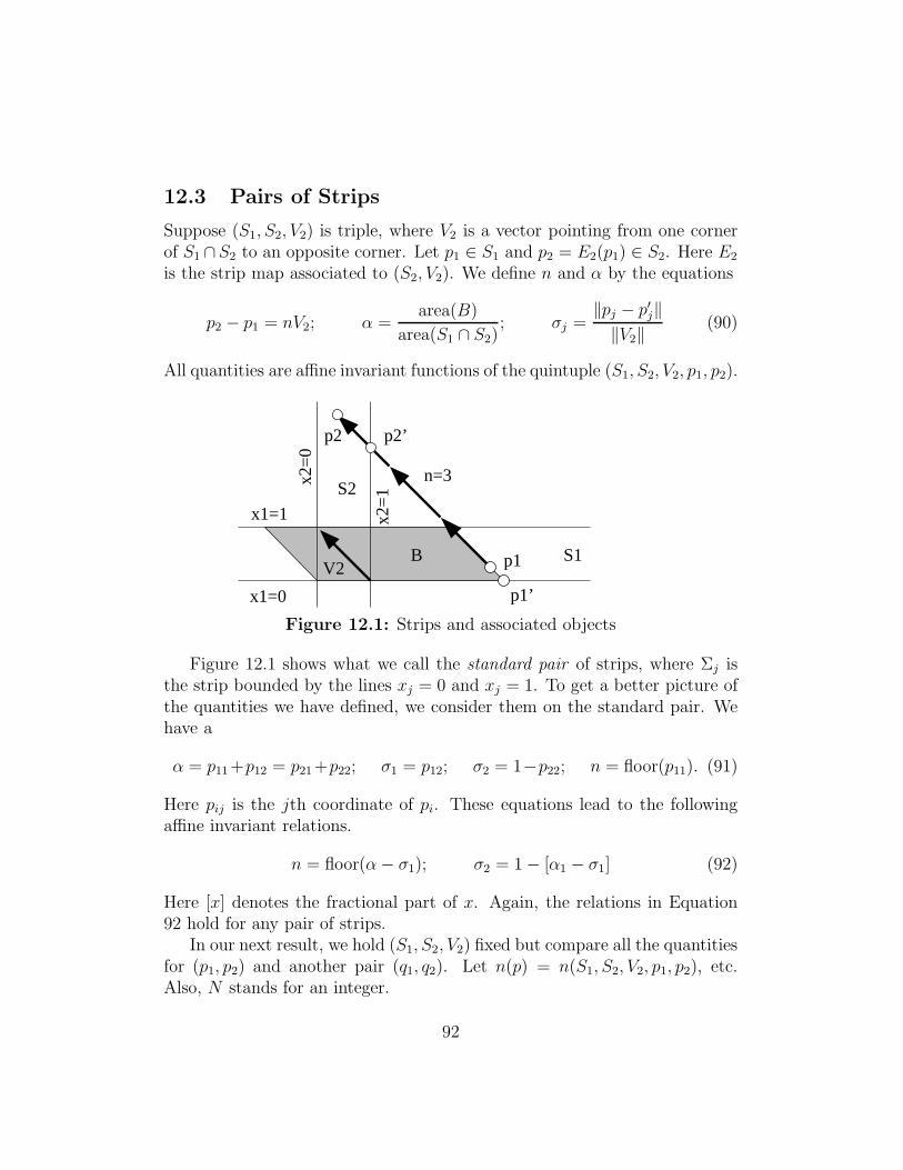
12.3 Pairs of Strips

Suppose (S1, S2, V2) is triple, where V2 is a vector pointing from one cornerof S1 ∩S2 to an opposite corner. Let p1 ∈ S1 and p2 = E2(p1) ∈ S2. Here E2

is the strip map associated to (S2, V2). We define n and α by the equations

p2 − p1 = nV2; α =area(B)

area(S1 ∩ S2); σj =

‖pj − p′j‖‖V2‖

(90)

All quantities are affine invariant functions of the quintuple (S1, S2, V2, p1, p2).

n=3x2=

0

p1’

p2’

x2=

1

x1=1

x1=0

V2B

p2

S2

S1p1

Figure 12.1: Strips and associated objects

Figure 12.1 shows what we call the standard pair of strips, where Σj isthe strip bounded by the lines xj = 0 and xj = 1. To get a better picture ofthe quantities we have defined, we consider them on the standard pair. Wehave a

α = p11+p12 = p21+p22; σ1 = p12; σ2 = 1−p22; n = floor(p11). (91)

Here pij is the jth coordinate of pi. These equations lead to the followingaffine invariant relations.

n = floor(α− σ1); σ2 = 1− [α1 − σ1] (92)

Here [x] denotes the fractional part of x. Again, the relations in Equation92 hold for any pair of strips.

In our next result, we hold (S1, S2, V2) fixed but compare all the quantitiesfor (p1, p2) and another pair (q1, q2). Let n(p) = n(S1, S2, V2, p1, p2), etc.Also, N stands for an integer.

92

Lemma 12.3 Let ǫ > 0. There is some δ > 0 with the following property.If |σ(p1)− σ(q1)| < δ and |α(q)−α(p)−N | < δ then |σ(p2)− σ(q2)| < ǫ andN = n(q) − n(p). The number δ only depends on ǫ and the distance fromσ(p1) and σ(p2) to {0, 1}.

Proof: If δ is small enough then [α(p)− σ(p1)] and [α(q)− σ(q1)] are veryclose, and relatively far from 0 or 1. Equation 92 now says that σ(p2) andσ(q2) are close. Also, the following two quantities are both near N while theindividual summands are all relatively far from integers.

α(q)− α(p);(α(q)− σ(q1)

)−

(α(p)− σ(p1)

)

But the second quantity is near the integer n(q)− n(p), by Equation 92. ♠

Suppose now that S1, S2, S3 is a triple of strips, and V2, V3 is a pair ofvectors, such that (S1, S2, V2) and (S2, S3, V3) are as above. Let pj ∈ Sj forj = 1, 2, 3 be such that p2 = E2(p1) and p3 = E3(p2). Define,

αj = α(Sj, Sj+1, Vj+1, pj , pj+1); j = 1, 2; λ =Area(S1 ∩ S2)

Area(S2 ∩ S3). (93)

It is convenient to set σ2 = σ(p2).

Lemma 12.4 There are constants C and D such that α2 = λα1 +Cσ2 +D.The constants C and D depend on the strips.

Proof: We normalize, as above, so that Equation 91 holds. Then

p2 = (1− σ2, α1 + σ2 − 1). (94)

There is a unique orientation preserving affine transformation T such thatT (Sj+1) = Sj for j = 1, 2, and T the line y = 1 to the line x = 0. Given thatS1 ∩ S2 has unit area, we have det(T ) = λ. Given the description of T , wehave

T (x, y) =(a λ−1 0

)(x, y) + (b, 1) = (ax+ b+ λy, 1− x). (95)

Here a and b are constants depending on S2∩S3. Setting q = T (p2), Equation91 gives α = q1 + q2. Hence

α2 = a(1− σ2) + b+ λ(α1 + σ2 − 1) + σ2 = λα1 + Cσ2 +D. (96)

This completes the proof. ♠

93

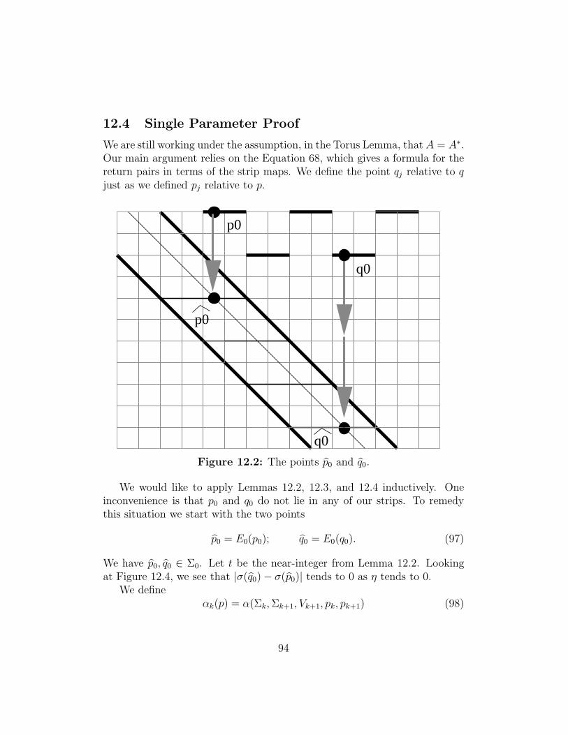
12.4 Single Parameter Proof

We are still working under the assumption, in the Torus Lemma, that A = A∗.Our main argument relies on the Equation 68, which gives a formula for thereturn pairs in terms of the strip maps. We define the point qj relative to qjust as we defined pj relative to p.

q0

p0

p0

q0

Figure 12.2: The points p0 and q0.

We would like to apply Lemmas 12.2, 12.3, and 12.4 inductively. Oneinconvenience is that p0 and q0 do not lie in any of our strips. To remedythis situation we start with the two points

p0 = E0(p0); q0 = E0(q0). (97)

We have p0, q0 ∈ Σ0. Let t be the near-integer from Lemma 12.2. Lookingat Figure 12.4, we see that |σ(q0)− σ(p0)| tends to 0 as η tends to 0.

We defineαk(p) = α(Σk,Σk+1, Vk+1, pk, pk+1) (98)

94

It is also convenient to write

σk(p) = σ(pk); ∆σk = σk(q)− σk(p). (99)

For k = 0, we use p0 in place of p0 and q0 in place of q0 for these formulas.

Lemma 12.5 As η → 0, the pairwise differences between the 3 quantities

αk(q)− αk(p); nk(q)− nk(p); tλk

converge to 0 for all k.

Proof: Referring to Figure 12.2, we have

Area(Σ0 ∩ Σ1) = 8; Area(B(p0))− Area(B(q0)) = 4y − 4x.

This gives us α0(q) − α0(p) = t. Applying Lemma 12.4 inductively, we findthat

αk = α0λk +k∑

i=1

ξiσi + Ck. (100)

for constants ξ1, ..., ξk and Ck that depend analytically on A. Therefore

αk(q)− αk(p) = tλk +k∑

i=1

ξi∆σi; k = 1, ..., 7 (101)

By Lemma 12.2, the term tλk is near an integer for all k. By Lemma 12.3and induction, the remaining terms on the right hand side are near 0. Thislemma now follows from Lemma 12.3. ♠

Combining our last result with Equation 87, we see that

n1(q)− n1(p) = n3(q)− n3(p) = n5(q)− n5(p) = n7(q)− n7(p);

n2(q)− n2(p) = n6(q)− n6(p). (102)

once η is small enough. Given the dependence of constants in Lemma 12.3,the necessary bound on η only depends on min(A, 1−A) and θ(p). Equation68 now tells us that ǫj(p) = ǫj(q) for j = 1, 2 once η is small enough.

95

12.5 A Generalization of Lemma 12.3

Now we turn to the proof of the Torus Lemma in the general case. Our firstresult is the key step that allows us to handle pairs of distinct parameters.Once we set up the notation, the proof is almost trivial. Our second resultis a variant that will be useful in the next chapter.

Suppose that (S1, S2, V2, p1, p2) and (S∗1 , S

∗2 , V

∗2 , q

∗1, q

∗2) are two quintu-

ples. To fix the picture in our minds we imagine that (S1, S2, V2) is near(S∗

1 , S∗2 , V

∗2 ), though this is not necessary for the proof of the result to follow.

We can define the quantities α, ρj, n for each of these quintuples. We put a(∗) by each quantity associated to the second triple.

Lemma 12.6 Let ǫ > 0. There is some δ > 0 with the following property.If |σ(p1)−σ(q∗1)| < δ and |α(q∗)−α(p)−N | < δ then |σ(p2)−σ(q∗2)| < ǫ andN = n(q∗) − n(p). The number δ only depends on ǫ and the distance fromσ(p1) and σ(p2) to {0, 1}.

Proof: There is an affine transformation such that T (X∗) = X for eachobject X = S1, S2, V2. We set qj = T (q∗j ). Then α(q∗1) = α(q1), by affineinvariance. Likewise for the other quantities. Now we apply Lemma 12.3to the triple (S1, S2, V2) and the pairs (p1, p2) and (q1, q2). The conclusioninvolves quantities with no (∗), but returning the (∗) does not change any ofthe quantities. ♠

For use in the next chapter, we state a variant of Lemma 12.6. Let [x]denote the image of x ∈ R/Z.

Lemma 12.7 Let ǫ > 0. There is some δ > 0 with the following property. If|σ(p1)−σ(q∗1)| < δ and |α(q∗)−α(p)−N | < δ then the distance from [σ(p2)]and [σ(q2)

∗] in R/Z is less than ǫ. |σ(p2)−σ(q∗2)| < ǫ and N = n(q∗)−n(p).The number δ only depends on ǫ and the distance from σ(p1) to {0, 1}.

Proof: Using the same trick as in Lemma 12.3, we reduce to the singlevariable case. In this case, we mainly repeat the proof of Lemma 12.3. Ifδ is small enough then [α(p) − σ(p1)] and [α(q)− σ(q1)] are very close, andrelatively far from 0 or 1. Equation 92 now says that [σ(p2)] and [σ(q2)] areclose in R/Z. ♠

96

12.6 Proof in the General Case

We no longer suppose that A = A∗, and we return to the original notation(q∗, A∗) for the second point. In our proof of this result, we attach a (∗) toany quantity that depends on (q∗, A∗). We first need to repeat the analysisfrom §12.2, this time keeping track of the parameter. Let η be as in theTorus Lemma. We use the big O notation.

Lemma 12.8 There is an integer Ik such that |α∗0λ

∗k − α0λk − Ik| < O(η).

Proof: Let [V ] denote the distance from V ∈ R3 to the nearest point inZ3. Let p = (x,±1) and q∗ = (x∗,±1). Recalling the definition of µ+, thehypotheses in the Torus Lemma imply that

[H∗

(x∗

2,x∗

2+ 1,

x∗

2

)−H

(x2,x

2+ 1,

x

2)]< O(η) (103)

We compute that α0 = x/2 + 1/2, independent of parameter. Therefore

H(x2,x

2+ 1,

x

2

)= H(α0, α0, α0) +

1

2H(−1, 1,−1).

The same goes with the starred quantities. Therefore,

[(λ∗2, λ∗

1 − 1, 1)α∗

0 − (λ2, λ1 − 1, 1)α0] =

[H∗(α∗

0, α∗

0, α∗

0)−H(α0, α0, α0)] < O(η) + ‖(H∗ −H)(−1, 1,−1)‖ < O(η).

Our lemma now follows immediately from Equation 87. ♠

The integer Ik of course depends on (p, A) and (q∗, A∗), but in all casesEquation 87 gives us

I0 = I4; I1 = I3 = I5 = I7; I2 = I6, (104)

Lemma 12.9 As η → 0, the pairwise differences between the 3 quantitiesα∗

k − αk and n∗k − nk and Ik tends to 0 for all k.

Proof: Here α∗k stands for αk(q

∗), etc. Equation 100 works separately foreach parameter. The replacement for Equation 101 is

α∗

k − αk = W +X + Y ; W = α∗

0λ∗

k − α0λk (105)

97

X =k∑

i=1

ξ∗i σ∗

i (q∗)−

k∑

i=1

ξiσi(p) =k∑

i=1

ξi(σ∗

i − σi) +O(|A− A∗|); (106)

Y =k∑

i=1

C∗

i −k∑

i=1

Ci = O(|A− A∗|). (107)

The estimates on X and Y comes from the fact ξi and Ci vary smoothly withA. Putting everything together, we get the following.

α∗

k − αk =(α∗

0λ∗

k − α0λk

)+

k∑

i=1

ξi(σ∗

i − σi) +O(|A− A∗|). (108)

In light of Lemma 12.8, it suffices to show that σ∗i − σi tends to 0 as η tends

to 0. The same argument as in the single parameter case works here, withLemma 12.6 used in place of Lemma 12.3. ♠

Similar to the single parameter case, Equations 68 and 104 now finish theproof.

98

13 The Strip Functions

13.1 The Main Result

The purpose of this chapter is to understand the functions σj that arose inthe proof of the Master Picture Theorem. We call these functions the stripfunctions .

Let Wk ⊂ Ξ+ × (0, 1) denote the set of points where Ek...E1 is definedbut Ek+1Ek...E1 is not defined. Let Sk denote the closure of µ+(Wk) in R.Finally, let

W ′

k =k−1⋃

j=0

Wj ; S ′

k =k−1⋃

j=0

Sj; k = 1, ..., 7. (109)

The Torus Lemma applies to any point that does not lie in the singular set

S = S0 ∪ ... ∪ S7. (110)

If p ∈ Ξ+ −W ′k then the points p = p0, ..., pk are defined. Here, as in

the previous chapter, pj = Ej(pj−1). The functions σ1, ..., σk and α1, ..., αk

are defined for such a choice of p. Again, σj measures the position of pj inΣj , relative to ∂Σj . Even if Ek+1 is not defined on pk, the equivalence class[pk+1] is well defined in the cylinder R2/〈Vk+1〉. The corresponding functionσk+1(q) = σ(qk+1) is well defined as an element of R/Z.

Let πj : R4 → R be the jth coordinate projection. Let [x] denote theimage of x in R/Z. The following identities refer to the (+) case. We discussthe (−) case at the end of the chapter.

σ1 =[2− π3

2

]◦ µ+ on Ξ+ (111)

σ2 =[1 + A− π2

1 + A

]◦ µ+ on Ξ+ −W ′

1 (112)

σ3 =[1 + A− π1

1 + A

]◦ µ+ on Ξ+ −W ′

2 (113)

σ4 =[1 + A− π1 − π2 + π3

2

]◦ µ+ on Ξ+ −W ′

3 (114)

In the next chapter we deduce the Master Picture Theorem from theseidentities and the Torus Lemma. In this chapter, we prove the identities.

99

13.2 Continuous Extension

Let g = σj for j = 0, ..., k + 1. since the image µ+(Ξ × (0, 1)) is dense inR− S ′

k, we define

g(τ) := limn→∞

g(pn, An); τ ∈ R− S ′

k. (115)

Here (pn, An) is chosen so that all functions are defined and µ+(pn, An)→ τ .Note that the sequence {pn} need not converge.

Lemma 13.1 The functions σ1, ..., σk+1, considered as R/Z-valued func-tions, are well defined and continuous on R − S ′

k.

Proof: For the sake of concreteness, we will give the proof in the case k = 2.This representative case explains the idea. First of all, the continuity followsfrom the well-definedness. We just have to show that the limit above is alwayswell defined. σ1 is well defined and continuous on all of R, by Equation 111.

Since S ′1 ⊂ S ′

2, we see that τ ∈ R − S ′1. Hence τ does not lie in the

closure of µ+(W0). Hence, there is some θ1 > 0 such that θ1(pn, An) > θ1 forall sufficiently large n. Note also that there is a positive and uniform lowerbound to min(An, 1− An). Note that [α1(pn, An)] = [π3(µ+(pn, An)]. Hence{[α1(pn, An)]} is a Cauchy sequence in R/Z.

Lemma 12.7 now applies uniformly to

(p, A) = (pm, Am); (q∗, A∗) = (pn, An)

for all sufficiently large pairs (m,n). Since {µ+(pn, An)} forms a Cauchy se-quence in R, Lemma 12.7 implies that {σ2(τm, Am)} forms a Cauchy sequencein R/Z. Hence, σ2 is well defined on R− S ′

1, and continuous.Since τ ∈ R − S ′

2, we see that τ does not lie in the closure of µ+(W1).Hence, there is some θ2 > 0 such that θj(pn, An) > θj for j = 1, 2 and all suf-ficiently large n. As in our proof of the General Torus Lemma, Equation 108now says that shows that {α2(pn, An)} forms a Cauchy sequence in R/Z. Wenow repeat the previous argument to see that {σ3(τm, Am)} forms a Cauchysequence in R/Z. Hence, σ3 is well defined on R− S ′

2, and continuous. ♠

Implicit in our proof above is the function

βk = [αk] ∈ R/Z. (116)

This function will come in handy in our next result.

100

13.3 Quality of the Extension

Let X = R− ∂R ⊂ R4. Note that X is open and convex

Lemma 13.2 Suppose X ⊂ R− S ′k. Then σk+1 is locally affine on XA.

Proof: Since σk+1 is continuous on X, it suffices to prove this lemma for adense set of A. We can choose A so that µ+(Ξ+) is dense in XA.

We already know that σ1, ..., σk+1 are all defined and continuous on X.We already remarked that Equation 111 is true by direct inspection. Aswe already remarked in the previous proof, β0 = π3 ◦ µ+. Thus, we defineβ0 = [π3]. Let β0 = [π3]. Both σ0 and β0 are locally affine on XA.

Let m ≤ k. The second half of Equation 92 tells us that σm is a locallyaffine function of σm−1 and βm−1. Below we will prove that βm is defined onXA, and locally affine, provided that σ1, ..., σm are locally affine. Our lemmafollows from this claim and induction.

Now we prove the claim. All the addition below is done in R/Z. Sinceµ+(Ξ+) is dense in XA, we can at least define βm on a dense subset of XA.Define

p = (x,±1); p′ = (x′,±1); τ = µ+(p); τ ′ = µ+(p′); t =x′ − x

2. (117)

We choose p and p′ so that the pinwheel map is entirely defined.From Equation 101, we have

βm(τ ′)− βm(τ) = [tλk] +m∑

j=1

[ξj × (σj(τ′)− σj(τ))]. (118)

Here ξ1, ..., ξm are constants that depend on A. Let H be the matrix inEquation 88. We have H(t, t, t) ≡ H(τ ′−τ) mod Z3 because (t, t, t) ≡ τ ′−τmod Λ. Our analysis in §12.2 shows that

[tλk] = [π ◦H(t, t, t)− ǫt] = [(π − ǫπ3) ◦H(τ ′ − τ)]. (119)

Here ǫ ∈ {0, 1} and π is some coordinate projection. The choice of ǫ and πdepends on k. We now see that

βm(τ ′) = βm(τ) + (π + ǫ3π) ◦H(τ ′ − τ) +m∑

j=1

[ξj × (σj(τ′)− σj(τ))]. (120)

The right hand side is everywhere defined and locally affine. Hence, we defineβm on all of XA using the right hand side of the last equation. ♠

101

Lemma 13.3 Suppose X ⊂ R− S ′k. Then σk+1 is analytic on X.

Proof: The constants ξj in Equation 118 vary analytically with A. Ourargument in Lemma 13.2 therefore shows that the linear part of σk+1 variesanalytically with A. We just have to check the linear term. Since XA isconnected we can compute the linear term of σk+1 at A from a single point.We choose p = (ǫ, 1) where ǫ is very close to 0. The fact that A→ σk(p, A)varies analytically follows from the fact that our strips vary analytically. ♠

Remark: We have Sk ⊂ σ−1k+1([0]). Given Equation 111, we see that

X ⊂ R − S ′1. Hence σ2 is defined on X. Hence σ2 is analyic on X and

locally affine on each XA. We use these two properties to show that Equa-tion 112 is true. But then X ⊂ R−S ′

2. etc. So, we will know at each stage ofour verification that Lemmas 13.2 and 13.3 apply to the function of interest.

Equations 112, 113, and 114 are formulas for σ2, σ3, and σ4 respectively.Let fk+1 = σk+1−σ′

k+1, where k = 2, 3, 4. Here σ′k+1 is the right hand side of

the identity for σk+1. Our goal is to show that fk+1 ≡ [0] for k = 1, 2, 3. Calla parameter A good if fk+1 ≡ [0] onXA. Call a subset S ⊂ (0, 1) substantial ifS is dense in some open interval of (0, 1). By analyticity, fk+1 ≡ [0] providedthat a substantial set of parameters is good.

In the next section we explain how to verify that a parameter is good.If fk+1 was a locally affine map from XA into R, we would just need tocheck that fk+1 = 0 on some tetrahedron on XA to verify that A is a goodparameter. Since the range of fk+1 is R/Z, we have to work a bit harder.

13.4 Irrational Quintuples

We will give a construction in R3. When the time comes to use the construc-tion, we will identify XA as an open subset of a copy of R3.

Let ζ1, ..., ζ5 ∈ R3 be 5 points. By taking these points 4 at a time, wecan compute 5 volumes, v1, ..., v5. Here vj is the volume of the tetrahedronobtained by omitting the jth point. We say that (ζ1, ..., ζ5) is an irrationalquintuple if the there is no rational relation

5∑

i=1

cjζj = 0; cj ∈ Q; c1c2c3c4c5 = 0. (121)

If we allow all the constants to be nonzero, then there is always a relation.

102

Lemma 13.4 Let C be an open convex subset of R3. Let f : C → R/Z bea locally affine function. Suppose that there is an irrational (ζ1, ..., ζ5) suchthat ζj ∈ C and f(ζj) is the same for all j. Then f is constant on C.

Proof: Since C is simply connected, we can lift f to a locally affine functionF : C → R. But then F is affinc on C, and we can extend F to be an affinemap from R3 to R. By construction F (ζi)− F (ζj) ∈ Z for all i, j. Addinga constant to F , we can assume that F is linear. There are several cases.

Case 1: Suppose that F (ζj) is independent of j. In this case, all the pointslie in the same plane, and all volumes are zero. This violates the irrationalitycondition.

Case 2: Suppose we are not in Case 1, and the following is true. For everyindex j there is a second index k such that F (ζk) = F (ζj). Since there are5 points total, this means that the set {F (ζj)} only has a total of 2 values.But this means that our 5 points lie in a pair of parallel planes, Π1 ∪ Π2,with 2 points in Π1 and 3 points in Π2. Let’s say that that ζ1, ζ2, ζ3 ∈ Π1

and ζ4, ζ5 ∈ Π2. But then v4 = v5, and we violate the irrationality condition.

Case 3: If we are not in the above two cases, then we can relabel so thatF (ζ1) 6= F (ζj) for j = 2, 3, 4, 5. Let

ζ ′j = ζj − ζ1.

Then ζ ′1 = (0, 0, 0) and F (ζ ′1) = 0. But then F (ζ ′j) ∈ Z−{0} for j = 2, 3, 4, 5.Note that v′j = vj for all j. For j = 2, 3, 4, 5, let

ζ ′′j =ζ ′j

F (ζ ′j).

Then v′′j /v′j ∈ Q for j = 2, 3, 4, 5. Note that F (ζ ′′j ) = 1 for j = 2, 3, 4, 5.

Hence there is a plane Π such that ζ ′′j ∈ Π for j = 2, 3, 4, 5.There is always a rational relation between the areas of the 4 triangles

defined by 4 points in the plane. Hence, there is a rational relation betweenv′′2 , v

′′3 , v

′′4 , v

′′5 . But then there is a rational relation between v2, v3, v4, v5. This

contradicts the irrationality condition. ♠

103

13.5 Verification in the Plus Case

Proceeding somewhat at random, we define

φj =(8jA+

1

2j, 1

); j = 1, 2, 3, 4, 5. (122)

We check that φj ∈ Ξ+ for A near 1/2. Letting ζj = µ+(φj), we check thatfk+1(ζj) = [0] for j = 1, 2, 3, 4, 5.

Example Calculation: Here is an example of what we do automatically inMathematica. Consider the case k = 1 and j = 1. When A = 1/2, the lengthspectrum for φ1 starts out (1, 1, 2, 1). Hence, this remains true for nearby A.Knowing the length spectrum allows us to compute, for instance, that

E2E1(φ1) = φ1 + V1 + V2 =(−3

2+ 8A, 7

)∈ Σ2

for A near 1/2. The affine functional

(x, y)→ (x, y, 1) · (−1, A, A)

2 + 2A(123)

takes on the value 0 on the line x = Ay+A and 1 on the line x = Ay−2−A.These are the two edges of Σ2. (See §15.1.) Therefore,

σ2(φ1) =(−3

2+ 8A, 7, 1

)· (−1, A, A)

2 + 2A=

3

4 + 4A.

At the same time, we compute that

µ+(φ1) =1

4(−7 + 24A, 1 + 4A,−7 + 16A),

at least for A near 1/2. When A is far from 1/2 this point will not lie in RA.We then compute

1 + A− π2(µ+(φ1))

1 + A=

3

4 + 4A.

This shows that f2(ζ2) = [0] for all A near 1/2. The verifications for theother pairs (k, j) are similar.

Checking Irrationality: It only remains to check that the points (ζ1, ..., ζ5)form an irrational quintuple for a dense set of parameters A. In fact this willtrue in the complement of a countable set of parameters.

The 5 volumes associated to our quintuple are as follows.

104

• v5 = 5/24− 5A/12 + 5A2/24.

• v4 = 71/40 + 19A/20− 787A2/120− 4A3.

• v3 = 119/60 + 7A/60− 89A2/15− 4A3

• v2 = −451/240− 13A/40 + 1349A2/240 + 4A3

• v1 = −167/80− 13A/40 + 533A2/80 + 4A3.

If there is an open set of parameters for which the first 4 of these volumes hasa rational relation, then there is an infinite set on which the same rationalrelation holds. Since every formula in sight is algebraic, this means that theremust be a single rational relation that holds for all parameters. But then thecurve A→ (v5, v4, v3, v2) lies in a proper linear subspace of R4.

We evaluate this curve at A = 1, 2, 3, 4 and see that the resulting pointsare linearly independent in R4. Hence, there is no global rational relation.Hence, on a dense set of parameters, there is no rational relation betweenthe first 4 volumes listed. A similar argument rules out rational relationsamongst any other 4-tuple of these volumes.

13.6 The Minus Case

In the (−) case, Equations 112 and 113 do not change, except that µ− replacesµ+ and all the sets are defined relative to Ξ− and µ−. Equations 111 and114 become

σ1 =[1− π3

2

]◦ µ− on Ξ−. (124)

σ4 =[A− π1 − π2 + π3

2

]◦ µ− on Ξ− − S ′

3. (125)

Lemma 13.2 and Lemma 13.3 have the same proof in the (−) case. We usethe same method as above, except that we use the points

φj + (2, 0); j = 1, 2, 3, 4, 5. (126)

These points all lie in Ξ− for A near 1/2. The rest of the verification isessentially the same as in the (+) case.

105

14 Proof of the Master Picture Theorem

14.1 The Main Argument

Let S be the singular set defined in Equation 110. Let S denote the unionof hyperplanes listed in §10.2. let d denote distance on the polytope R. Inthis chapter we will prove

Lemma 14.1 (Hyperplane) S ⊂ S and θ(p, A) ≥ d(µ+(p, A), S).

We finish the proof of the Master Picture Theorem assuming the Hyper-plane Lemma.

Say that a ball of constancy in R − S is an open ball B with the fol-lowing property. If (p0, A0) and (p1, A1) are two pairs and µ+(pj, Ak) ∈ Bfor j = 0, 1, then (p0, A0) and (p1, A1) have the same return pair. Here is aconsequence of the Torus Lemma.

Corollary 14.2 Any point τ of R− S is contained in a ball of constancy.

Proof: If τ is in the image of µ+, this result is an immediate consequenceof the Torus Lemma. In general, the image µ+(Ξ+ × (0, 1)) is dense in R.Hence, we can find a sequence {τn} such that τn → τ and τn = µ+(pn, An).Let 2θ0 > 0 be the distance from τ to S. From the triangle inequality andthe second statement of the Hyperplane Lemma, θ(pn, An) ≥ θ0 = θ1 > 0for large n. By the Torus Lemma, τn is the center of a ball Bn of constancywhose radius depends only on θ0. In particular – and this is really all thatmatters in our proof – the radius of Bn does not tend to 0. Hence, for n largeenough, τ itself is contained in Bn. ♠

Lemma 14.3 Let (p0, A0) and (p1, A1) be two points of Ξ+× (0, 1) such thatµ+(p0, A0) and µ+(p1, A1) lie in the same path connected component of R−S.Then the return pair for (p0, A0) equals the return pair for (p1, A1).

Proof: Let L ⊂ R − S be a path joining points τ0 = µ+(p0, A0) andτ1 = µ+(p1, A1). By compactness, we can cover L by finitely many over-lapping balls of constancy. ♠

106

Now we just need to see that the Master Picture Theorem holds for onecomponent of the partition of R − S. Here is an example calculation thatdoes the job. For each α = j/16 for j = 1, ..., 15, we plot the image

µA(2α + 2n); n = 1, ..., 215; (127)

The image is contained in the slice z = α. We see that the Master PictureTheorem holds for all these points. The reader can use Billiard King to plotand inspect millions of points for any desired parameter.

We have really only proved the half of the Master Picture Theorem thatdeals with Ξ+ and µ+. The half that deals with Ξ− and µ− is exactly thesame. In particular, both the Torus Lemma and the Hyperplane Lemma holdverbatim in the (−) case. The proof of the Hyperplane Lemma in the (−)case differs only in that the two identities in Equation 124 replace Equations111 and 114. We omit the details in the (−) case.

14.2 The First Four Singular Sets

Our strip function identites make short work of the first four pieces of thesingular set.

• Given Equation 111,

S0 ⊂ {z = 0} ∪ {z = 1}. (128)

• Given Equation 112,

S1 ⊂ {y = 0} ∪ {y = 1 + A}. (129)

• Given Equation 113,

S2 ⊂ {x = 0} ∪ {x = 1 + A}. (130)

• Give Equation 114,

S3 ⊂ {x+ y − z = 1 + A} ∪ {x+ y − z = −1 + A}. (131)

107

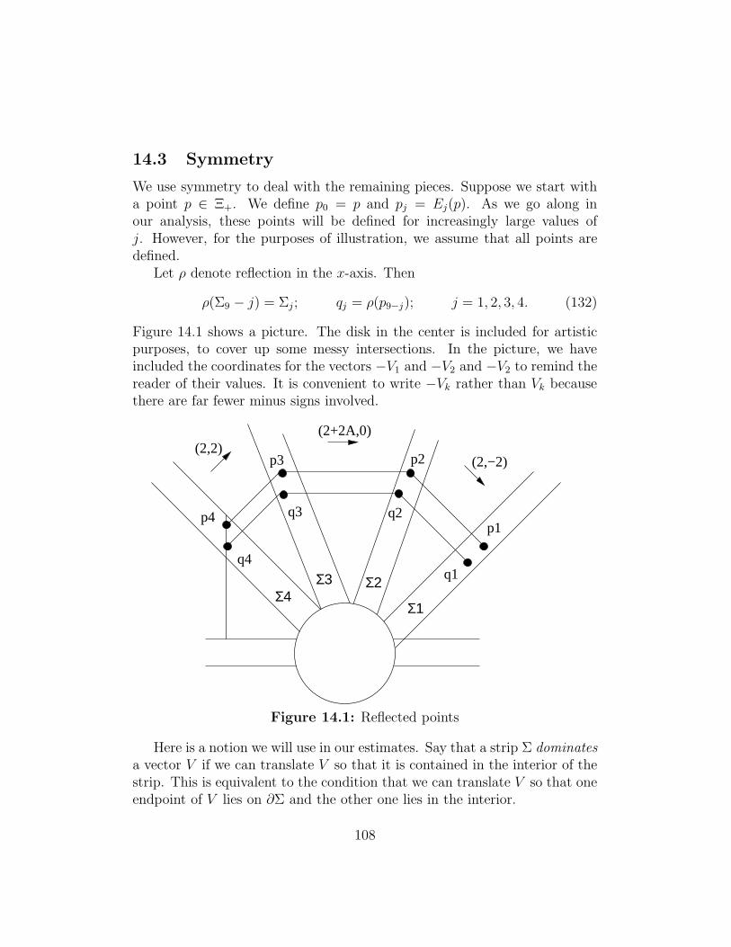
14.3 Symmetry

We use symmetry to deal with the remaining pieces. Suppose we start witha point p ∈ Ξ+. We define p0 = p and pj = Ej(p). As we go along inour analysis, these points will be defined for increasingly large values ofj. However, for the purposes of illustration, we assume that all points aredefined.

Let ρ denote reflection in the x-axis. Then

ρ(Σ9 − j) = Σj ; qj = ρ(p9−j); j = 1, 2, 3, 4. (132)

Figure 14.1 shows a picture. The disk in the center is included for artisticpurposes, to cover up some messy intersections. In the picture, we haveincluded the coordinates for the vectors −V1 and −V2 and −V2 to remind thereader of their values. It is convenient to write −Vk rather than Vk becausethere are far fewer minus signs involved.

Σ2

(2,−2)

(2+2A,0)(2,2)

q4

Σ4Σ1

Σ3

p2

q2p1

q1

q3p4

p3

Figure 14.1: Reflected points

Here is a notion we will use in our estimates. Say that a strip Σ dominatesa vector V if we can translate V so that it is contained in the interior of thestrip. This is equivalent to the condition that we can translate V so that oneendpoint of V lies on ∂Σ and the other one lies in the interior.

108

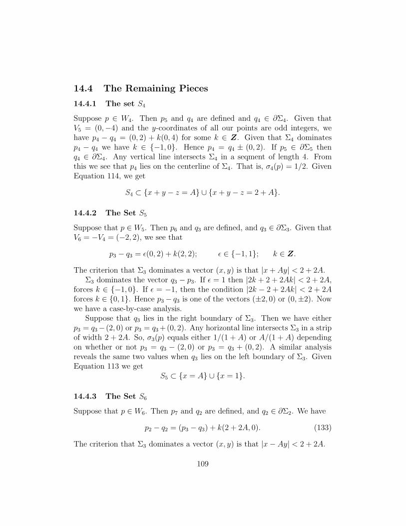
14.4 The Remaining Pieces

14.4.1 The set S4

Suppose p ∈ W4. Then p5 and q4 are defined and q4 ∈ ∂Σ4. Given thatV5 = (0,−4) and the y-coordinates of all our points are odd integers, wehave p4 − q4 = (0, 2) + k(0, 4) for some k ∈ Z. Given that Σ4 dominatesp4 − q4 we have k ∈ {−1, 0}. Hence p4 = q4 ± (0, 2). If p5 ∈ ∂Σ5 thenq4 ∈ ∂Σ4. Any vertical line intersects Σ4 in a seqment of length 4. Fromthis we see that p4 lies on the centerline of Σ4. That is, σ4(p) = 1/2. GivenEquation 114, we get

S4 ⊂ {x+ y − z = A} ∪ {x+ y − z = 2 + A}.

14.4.2 The Set S5

Suppose that p ∈W5. Then p6 and q3 are defined, and q3 ∈ ∂Σ3. Given thatV6 = −V4 = (−2, 2), we see that

p3 − q3 = ǫ(0, 2) + k(2, 2); ǫ ∈ {−1, 1}; k ∈ Z.

The criterion that Σ3 dominates a vector (x, y) is that |x+ Ay| < 2 + 2A.Σ3 dominates the vector q3 − p3. If ǫ = 1 then |2k + 2 + 2Ak| < 2 + 2A,

forces k ∈ {−1, 0}. If ǫ = −1, then the condition |2k − 2 + 2Ak| < 2 + 2Aforces k ∈ {0, 1}. Hence p3− q3 is one of the vectors (±2, 0) or (0,±2). Nowwe have a case-by-case analysis.

Suppose that q3 lies in the right boundary of Σ3. Then we have eitherp3 = q3− (2, 0) or p3 = q3 +(0, 2). Any horizontal line intersects Σ3 in a stripof width 2 + 2A. So, σ3(p) equals either 1/(1 + A) or A/(1 + A) dependingon whether or not p3 = q3 − (2, 0) or p3 = q3 + (0, 2). A similar analysisreveals the same two values when q3 lies on the left boundary of Σ3. GivenEquation 113 we get

S5 ⊂ {x = A} ∪ {x = 1}.

14.4.3 The Set S6

Suppose that p ∈W6. Then p7 and q2 are defined, and q2 ∈ ∂Σ2. We have

p2 − q2 = (p3 − q3) + k(2 + 2A, 0). (133)

The criterion that Σ3 dominates a vector (x, y) is that |x− Ay| < 2 + 2A.

109

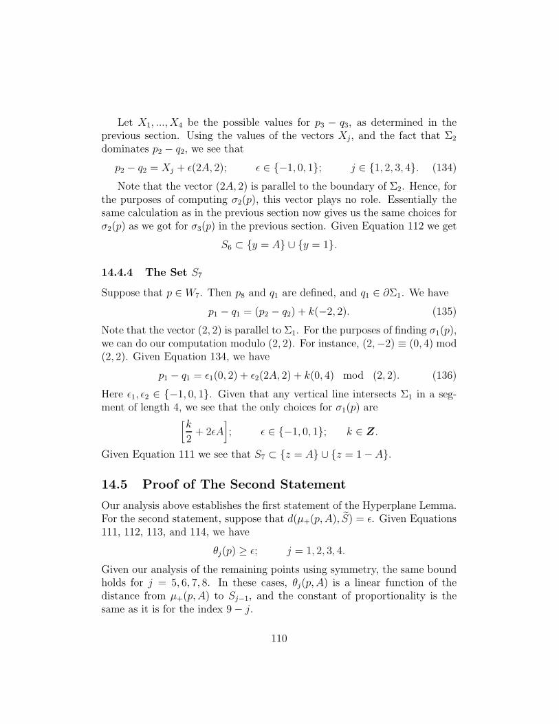
Let X1, ..., X4 be the possible values for p3 − q3, as determined in theprevious section. Using the values of the vectors Xj, and the fact that Σ2

dominates p2 − q2, we see that

p2 − q2 = Xj + ǫ(2A, 2); ǫ ∈ {−1, 0, 1}; j ∈ {1, 2, 3, 4}. (134)

Note that the vector (2A, 2) is parallel to the boundary of Σ2. Hence, forthe purposes of computing σ2(p), this vector plays no role. Essentially thesame calculation as in the previous section now gives us the same choices forσ2(p) as we got for σ3(p) in the previous section. Given Equation 112 we get

S6 ⊂ {y = A} ∪ {y = 1}.

14.4.4 The Set S7

Suppose that p ∈W7. Then p8 and q1 are defined, and q1 ∈ ∂Σ1. We have

p1 − q1 = (p2 − q2) + k(−2, 2). (135)

Note that the vector (2, 2) is parallel to Σ1. For the purposes of finding σ1(p),we can do our computation modulo (2, 2). For instance, (2,−2) ≡ (0, 4) mod(2, 2). Given Equation 134, we have

p1 − q1 = ǫ1(0, 2) + ǫ2(2A, 2) + k(0, 4) mod (2, 2). (136)

Here ǫ1, ǫ2 ∈ {−1, 0, 1}. Given that any vertical line intersects Σ1 in a seg-ment of length 4, we see that the only choices for σ1(p) are

[k

2+ 2ǫA

]; ǫ ∈ {−1, 0, 1}; k ∈ Z.

Given Equation 111 we see that S7 ⊂ {z = A} ∪ {z = 1−A}.

14.5 Proof of The Second Statement

Our analysis above establishes the first statement of the Hyperplane Lemma.For the second statement, suppose that d(µ+(p, A), S) = ǫ. Given Equations111, 112, 113, and 114, we have

θj(p) ≥ ǫ; j = 1, 2, 3, 4.

Given our analysis of the remaining points using symmetry, the same boundholds for j = 5, 6, 7, 8. In these cases, θj(p, A) is a linear function of thedistance from µ+(p, A) to Sj−1, and the constant of proportionality is thesame as it is for the index 9− j.

110

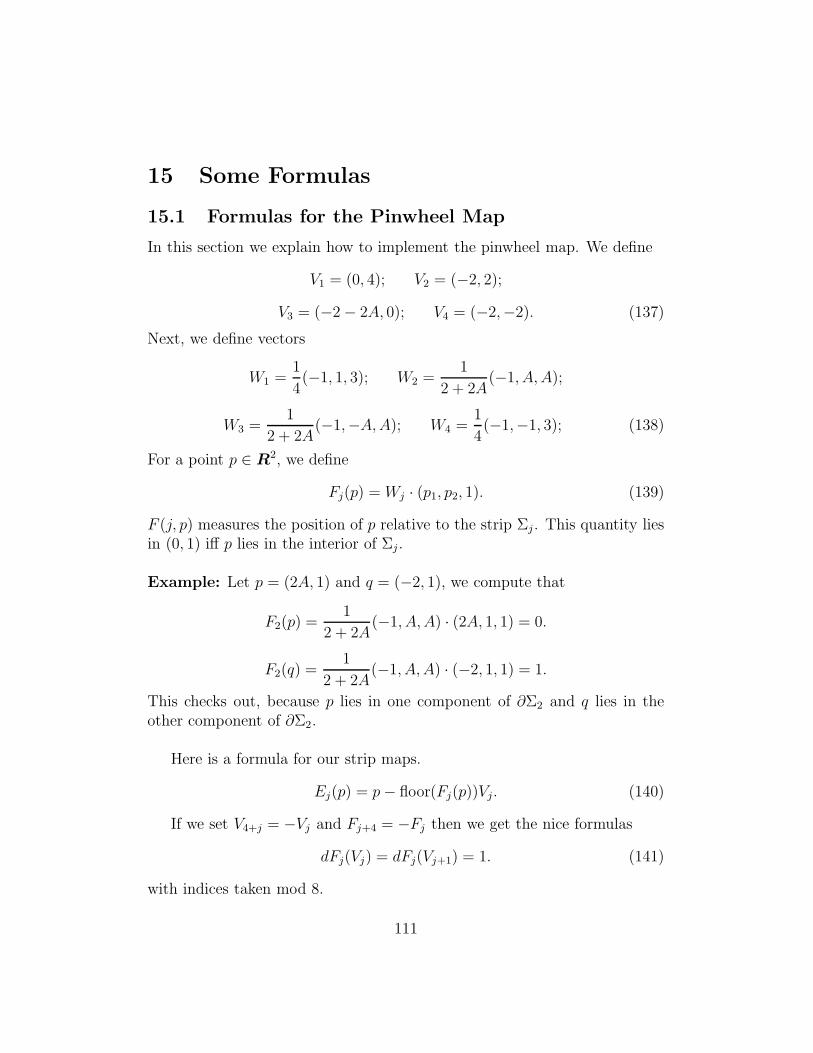
15 Some Formulas

15.1 Formulas for the Pinwheel Map

In this section we explain how to implement the pinwheel map. We define

V1 = (0, 4); V2 = (−2, 2);

V3 = (−2− 2A, 0); V4 = (−2,−2). (137)

Next, we define vectors

W1 =1

4(−1, 1, 3); W2 =

1

2 + 2A(−1, A, A);

W3 =1

2 + 2A(−1,−A,A); W4 =

1

4(−1,−1, 3); (138)

For a point p ∈ R2, we define

Fj(p) = Wj · (p1, p2, 1). (139)

F (j, p) measures the position of p relative to the strip Σj . This quantity liesin (0, 1) iff p lies in the interior of Σj .

Example: Let p = (2A, 1) and q = (−2, 1), we compute that

F2(p) =1

2 + 2A(−1, A, A) · (2A, 1, 1) = 0.

F2(q) =1

2 + 2A(−1, A, A) · (−2, 1, 1) = 1.

This checks out, because p lies in one component of ∂Σ2 and q lies in theother component of ∂Σ2.

Here is a formula for our strip maps.

Ej(p) = p− floor(Fj(p))Vj. (140)

If we set V4+j = −Vj and Fj+4 = −Fj then we get the nice formulas

dFj(Vj) = dFj(Vj+1) = 1. (141)

with indices taken mod 8.

111

15.2 The Reduction Algorithm

Let A ∈ (0, 1) and α ∈ R+ and (m,n) ∈ Z2 be a point above the baseline ofΓα(A). In this section we describe how we compute the points

µ±(Mα(m,n)).

This algorithm will be important when we prove the Copy Theorems in PartIV of the monograph.

1. Let z = Am+ n+ α.

2. Let Z = floor(z).

3. Let y = z + Z.

4. Let Y = floor(y/(1 + A)).

5. Let x = y − Y (1− A)− 1.

6. Let X = floor(x/(1 + A)).

We then have

µ−(Mα(m,n)) =

x− (1 + A)Xy − (1 + A)Y

z − Z

(142)

The description of µ+ is identical, except that the third step above is replacedby

y = z + Z + 1. (143)

Example: Referring to §10.4, consider the case when A = 3/5 and α = 1/10and (m,n) = (4, 2). We get

z =9

2; Z = 4; y =

17

2; Y = floor

(17/2

8/5

)= 5.

x =17

2− 5(

2

5)− 1 =

11

2; X = floor

(11/2

8/5

)= 3.

µ−(M(4, 2)) =(11

2− 3(

8

5),

17

2− 5(

8

5),

9

2− 4

)=

( 7

10,1

2,1

2

).

112

15.3 Computing the Partition

Here we describe how Billiard King applies the Master Picture Theorem.

15.3.1 Step 1

Suppose (a, b, c) ∈ RA lies in the range of µ+ or µ−. Now we describe howto attach a 5-tuple (n0, .., n4) to (a, b, c).

• Determining n0:

– If we are interested in µ+, then n0 = 0.

– If we are interested in µ−, then n0 = 1.

• Determining n1:

– If c < A and c < 1− A then n1 = 0.

– If c > A and c < 1− A then n1 = 1.

– If c > A and c > 1− A then n1 = 2.

– If c < A and c > 1− A then n1 = 3.

• Determining n2:

– If a ∈ (0, A) then n2 = 0.

– If a ∈ (A, 1) then n2 = 1.

– If a ∈ (1, 1 + A) then n2 = 2.

• Determining n3.

– If b ∈ (0, A) then n3 = 0.

– If b ∈ (A, 1) then n3 = 1.

– If b ∈ (1, 1 + A) then n3 = 2.

• Determining n4.

– Let t = a + b− c.– Let n4 = floor(t−A).

Notice that each 5-tuple (n0, ..., n4) corresponds to a (possibly empty) convexpolyhedron in RA. The polyhedron doesnt depend on n0. It turns out thatthis polyhedron is empty unless n4 ∈ {−2,−1, 0, 1, 2}.

113

15.3.2 Step 2

Let n = (n0, ..., n4). We now describe two functions ǫ1(n) ∈ {−1, 0, 1} andǫ2(n) ∈ {−1, 0, 1}.

Here is the definition of ǫ1(n).

• If n0 + n4 is even then:

– If n2 + n3 = 4 or x2 < x3 set ǫ1(n) = −1.

• If n0 + n4 is odd then:

– If n2 + n3 = 0 or x2 > x3 set ǫ1(n) = +1.

• Otherwise set ǫ1(n) = 0.

Here is the definition of ǫ2(n).

• If n0 = 0 and n1 ∈ {3, 0}.

– If n2 = 0 let ǫ2(n) = 1.

– If n2 = 1 and n4 6= 0 let ǫ2(n) = 1.

• If n0 = 1 and n1 ∈ {0, 1}.

– if n2 > 0 and n4 6= 0 let ǫ2(n) = −1.

– If n2 < 2 and n3 = 0 and n4 = 0 let ǫ2(n) = 1.

• If n0 = 0 and n1 ∈ {1, 2}.

– If n2 < 2 and n4 6= 0 let ǫ2(n) = 1.

– If n2 > 0 and n3 = 2 and n4 = 0 let ǫ2(n) = −1.

• If n0 = 1 and n1 ∈ {2, 3}.

– If n2 = 2 let ǫ2(n) = −1.

– If n2 = 1 and n4 6= 0 let ǫ2(n) = −1.

• Otherwise let ǫ2(n) = 0.

114

15.3.3 Step 3

Let A ∈ (0, 1) be any parameter and let α > 0 be some parameter suchthat α 6∈ 2Z[A]. Given any lattice point (m,n) we perform the followingconstruction.

• Let (a±, b±, c±) = µ±(A,m, n). See §15.2.

• Let n± be the 5-tuple associated to (a±, b±, c±).

• Let ǫ±1 = ǫ1(n±) and ǫ±2 = ǫ2(n±).

The Master Picture Theorem says that the two edges of Γα(m,n) incidentto (m,n) are (m,n) + (ǫ±1 , ǫ

±

2 ).

15.4 The List of Polytopes

Referring to the simpler partition from §10.6, we list the 14 polytopes thatpartition R+. In each case, we list some vectors, followed by the pair (ǫ1, ǫ2)that the polytope determines.

0000

0001

0010

0101

0111

1001

1010

1011

1111

(1, 1)

0000

0100

0101

0201

0211

1101

1111

1211

(−1, 1)

0100

0110

1110

1111

1211

2111

(−1,−1)

0100

0201

1000

1100

1101

1110

1201

1211

(0, 1)

0000

0010

0101

0110

0111

0211

1010

1111

(0, 1)

115

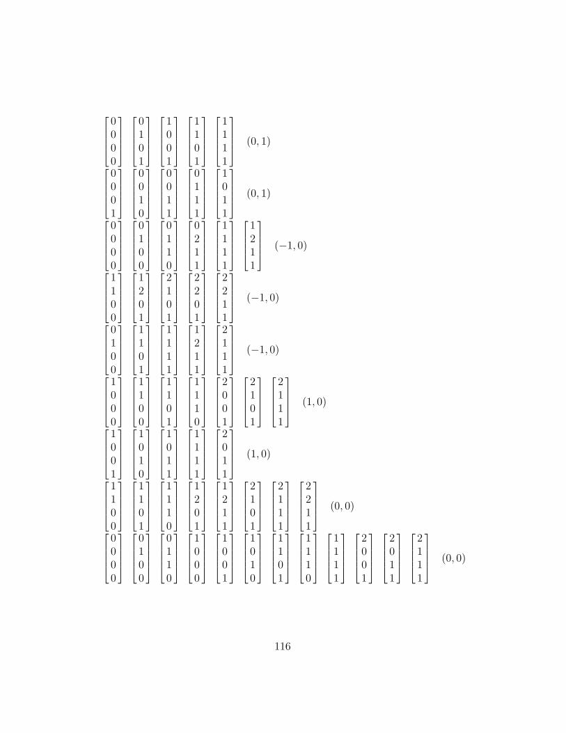
0000

0101

1001

1101

1111

(0, 1)

0001

0010

0011

0111

1011

(0, 1)

0000

0100

0110

0211

1111

1211

(−1, 0)

1100

1201

2101

2201

2211

(−1, 0)

0100

1101

1111

1211

2111

(−1, 0)

1000

1100

1101

1110

2001

2101

2111

(1, 0)

1001

1010

1011

1111

2011

(1, 0)

1100

1101

1110

1201

1211

2101

2111

2211

(0, 0)

0000

0100

0110

1000

1001

1010

1101

1110

1111

2001

2011

2111

(0, 0)

116

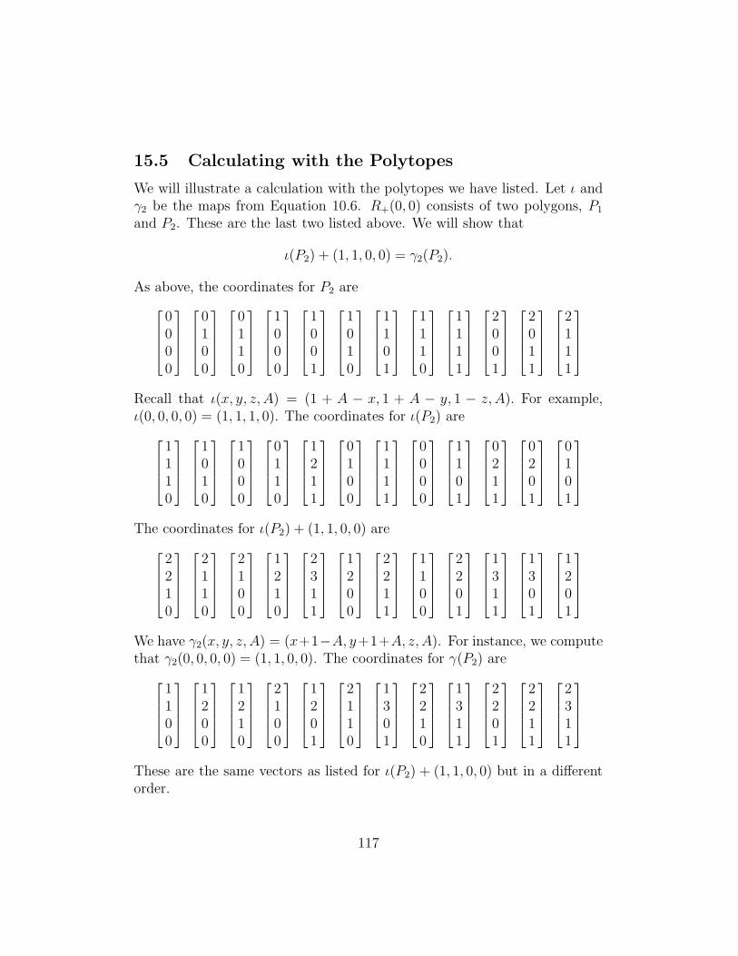
15.5 Calculating with the Polytopes

We will illustrate a calculation with the polytopes we have listed. Let ι andγ2 be the maps from Equation 10.6. R+(0, 0) consists of two polygons, P1

and P2. These are the last two listed above. We will show that

ι(P2) + (1, 1, 0, 0) = γ2(P2).

As above, the coordinates for P2 are

0000

0100

0110

1000

1001

1010

1101

1110

1111

2001

2011

2111

Recall that ι(x, y, z, A) = (1 + A − x, 1 + A − y, 1 − z, A). For example,ι(0, 0, 0, 0) = (1, 1, 1, 0). The coordinates for ι(P2) are

1110

1010

1000

0110

1211

0100

1111

0000

1101

0211

0201

0101

The coordinates for ι(P2) + (1, 1, 0, 0) are

2210

2110

2100

1210

2311

1200

2211

1100

2201

1311

1301

1201

We have γ2(x, y, z, A) = (x+1−A, y+1+A, z, A). For instance, we computethat γ2(0, 0, 0, 0) = (1, 1, 0, 0). The coordinates for γ(P2) are

1100

1200

1210

2100

1201

2110

1301

2210

1311

2201

2211

2311

These are the same vectors as listed for ι(P2) + (1, 1, 0, 0) but in a differentorder.

117

Part IIIIn this part of the monograph we use the Master Picture Theorem to

prove most of the results we quoted in Part I of the monograph.

• In §16 we prove the Embedding Theorem.

• In §17 we prove some results about the symmetries of the arithmeticgraph and the hexagrid.

• In §18 we establish some information about the doors. These specialpoints were defined in connection with the Hexagrid Theorem.

• In §19 we prove Statement 1 of the Hexagrid theorem, namely that thearithmetic graph does not cross any floor lines.

• In §20 we prove Statement 2 of the Hexagrid theorem, namely that thearithmetic graph only crosses the walls near the doors. The two state-ments of the Hexagrid Theorem have similar proofs, though Statement2 has a more elaborate proof.

Many of the proofs in this part of the monograph require us to prove var-ious disjointness results about some 4 dimensional polytopes. We will giveshort computer-aided proofs of these disjointness results. The proofs onlyinvolve a small amount of integer arithmetic. An energetic mathematiciancould do them all by hand in an afternoon. To help make the proofs sur-veyable, we will include extensive computer pictures of 2 dimensional slicesof our polytopes. These pictures, all reproducible on Billiard King, serve assanity checks for the computer calculations.

118

16 Proof of the Embedding Theorem

Let Γ = Γα(A) be the arithmetic graph for a parameter A and some numberα 6∈ 2Z[A]. In this chapter we prove that Γ is a disjoint union of embeddedpolygons and infinite polygonal arcs. This is the Embedding Theorem.

16.1 Step 1

We will first prove that every nontrivial vertex of Γ has valence 2. Each pointp ∈ Γ is connected to two points q+ and q−. Hence, each non-trivial vertexhas valence either 1 or 2. The following two cases are the only cases thatlead to valence 1 vertices:

• p = q+ and q+ 6= q−.

• q+ = q− and q± 6= p.

The following lemma rules out the first of these cases.

Lemma 16.1 If p = q+ or p = q− then p = q+ = q−.

Proof: Our proof refers to §10.6. Recall that R+(0, 0) consists of 2 convexinteger polytopes. Likewise R−(0, 0) consists of 2 convex integer polytopes.It suffices to show that

(t, t+ 1, t) ∈ R+(0, 0) ⇐⇒ (t− 1, t, t) ∈ R−(0, 0). (144)

This is equivalent to the statement that

R−(0, 0) + (1, 1, 0, 0) ⊂ ΛR+(0, 0)

Here ΛR+(0, 0) is the orbit of R+(0, 0) under the action of Λ. Let ι be theinvolution from Equation 57. Recall that R−(0, 0) = ι(R+(0, 0)). Hence,Equation 144 equivalent to the statement that

ι(R+(0, 0)) + (1, 1, 0, 0) ⊂ ΛR+(0, 0). (145)

Let P1 and P2 denote the two polytopes comprising R+(0, 0), as listed at theend of §10. Let γ2 be the element of Λ described in §10.6. We compute that

ι(P1) + (1, 1, 0, 0) = P1; ι(P2) + (1, 1, 0, 0)) = γ2(P2). (146)

We did the second calculation in §15.5, and the first computation is similar.This does it for us. ♠

119

16.2 Step 2

Our next goal is to rule out the possibility that p 6= q±, but q+ = q−. Thissituation happens iff there is some (ǫ1, ǫ2) ∈ {−1, 0, 1} such that

ΛR+(ǫ1, ǫ2) ∩ (R−(ǫ1, ǫ2) + (1, 1, 0, 0)) 6= ∅. (147)

A visual inspection and/or a compute computer search – we did both –reveals that at least one of the two sets above is empty unless (ǫ1, ǫ2) is oneof

(1, 1); (−1,−1); (1, 0); (−1, 0). (148)

To rule out Equation 147 for each of these pairs, we need to consider allpossible pairs (P1, P2) of integral convex polytopes such that

P1 ⊂ ΛR+(ǫ1, ǫ2); P2 ⊂ (R−(ǫ1, ǫ2) + (1, 1)) (149)

Recall that Λ is generated by the three elements γ1, γ2, γ3. Let Λ′ ⊂ Λ denotethe subgroup generated by γ1 and γ2. We also define Λ′

10 ⊂ Λ′ by the equation

Λ′

10 = {a1γ1 + a2γ2| |a1|, |a2| ≤ 10}. (150)

Lemma 16.2 Let γ ∈ Λ− Λ′. Suppose that

P1 = γ(Q1); Q1 ⊂ R+(ǫ1, ǫ2); P2 ⊂ R−(ǫ1, ǫ2) + (1, 1, 0, 0).

Then P1 and P2 have disjoint interiors.

Proof: The third coordinates of points in P1 lies between n and n + 1 forsome n 6= 0 whereas the third coordinates of points in P2 lie in [0, 1]. ♠

Lemma 16.3 Let γ ∈ Λ′ − Λ′10.

P1 = γ(Q1); Q1 ⊂ R+(ǫ1, ǫ2); P2 ⊂ R−(ǫ1, ǫ2) + (1, 1, 0, 0).

Then P1 and P2 have disjoint interiors.

Proof: Q1 is contained in the ball of radius 4 about P2, but γ moves thisball entirely off itself. ♠

120

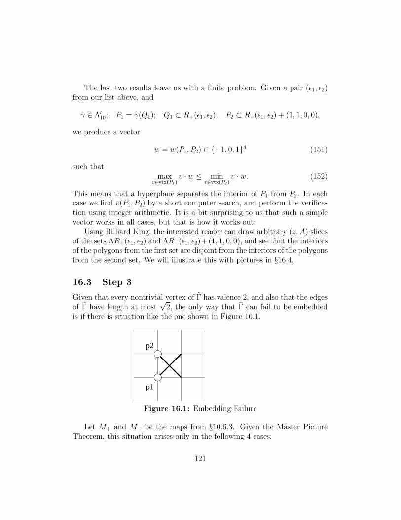
The last two results leave us with a finite problem. Given a pair (ǫ1, ǫ2)from our list above, and

γ ∈ Λ′

10; P1 = γ(Q1); Q1 ⊂ R+(ǫ1, ǫ2); P2 ⊂ R−(ǫ1, ǫ2) + (1, 1, 0, 0),

we produce a vector

w = w(P1, P2) ∈ {−1, 0, 1}4 (151)

such thatmax

v∈vtx(P1)v · w ≤ min

v∈vtx(P2)v · w. (152)

This means that a hyperplane separates the interior of P1 from P2. In eachcase we find v(P1, P2) by a short computer search, and perform the verifica-tion using integer arithmetic. It is a bit surprising to us that such a simplevector works in all cases, but that is how it works out.

Using Billiard King, the interested reader can draw arbitrary (z, A) slicesof the sets ΛR+(ǫ1, ǫ2) and ΛR−(ǫ1, ǫ2)+(1, 1, 0, 0), and see that the interiorsof the polygons from the first set are disjoint from the interiors of the polygonsfrom the second set. We will illustrate this with pictures in §16.4.

16.3 Step 3

Given that every nontrivial vertex of Γ has valence 2, and also that the edgesof Γ have length at most

√2, the only way that Γ can fail to be embedded

is if there is situation like the one shown in Figure 16.1.

p2

p1

Figure 16.1: Embedding Failure

Let M+ and M− be the maps from §10.6.3. Given the Master PictureTheorem, this situation arises only in the following 4 cases:

121

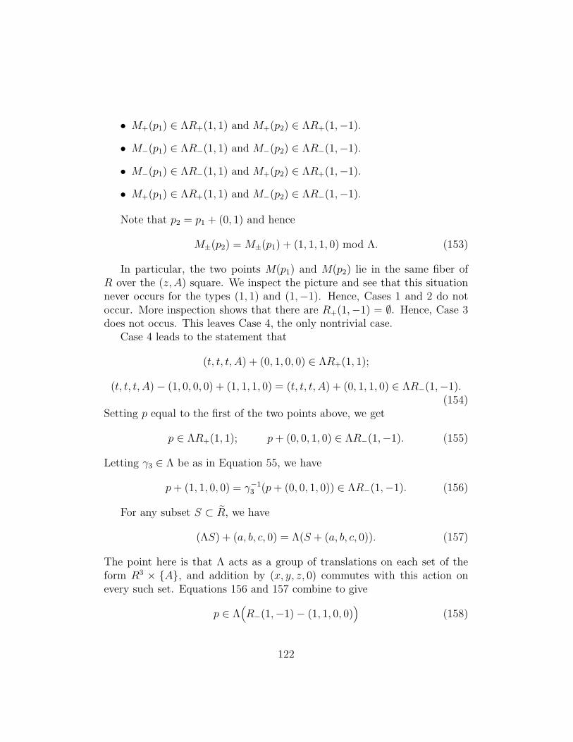
• M+(p1) ∈ ΛR+(1, 1) and M+(p2) ∈ ΛR+(1,−1).

• M−(p1) ∈ ΛR−(1, 1) and M−(p2) ∈ ΛR−(1,−1).

• M−(p1) ∈ ΛR−(1, 1) and M+(p2) ∈ ΛR+(1,−1).

• M+(p1) ∈ ΛR+(1, 1) and M−(p2) ∈ ΛR−(1,−1).

Note that p2 = p1 + (0, 1) and hence

M±(p2) = M±(p1) + (1, 1, 1, 0) mod Λ. (153)

In particular, the two points M(p1) and M(p2) lie in the same fiber ofR over the (z, A) square. We inspect the picture and see that this situationnever occurs for the types (1, 1) and (1,−1). Hence, Cases 1 and 2 do notoccur. More inspection shows that there are R+(1,−1) = ∅. Hence, Case 3does not occus. This leaves Case 4, the only nontrivial case.

Case 4 leads to the statement that

(t, t, t, A) + (0, 1, 0, 0) ∈ ΛR+(1, 1);

(t, t, t, A)− (1, 0, 0, 0) + (1, 1, 1, 0) = (t, t, t, A) + (0, 1, 1, 0) ∈ ΛR−(1,−1).(154)

Setting p equal to the first of the two points above, we get

p ∈ ΛR+(1, 1); p+ (0, 0, 1, 0) ∈ ΛR−(1,−1). (155)

Letting γ3 ∈ Λ be as in Equation 55, we have

p+ (1, 1, 0, 0) = γ−13 (p+ (0, 0, 1, 0)) ∈ ΛR−(1,−1). (156)

For any subset S ⊂ R, we have

(ΛS) + (a, b, c, 0) = Λ(S + (a, b, c, 0)). (157)

The point here is that Λ acts as a group of translations on each set of theform R3 × {A}, and addition by (x, y, z, 0) commutes with this action onevery such set. Equations 156 and 157 combine to give

p ∈ Λ(R−(1,−1)− (1, 1, 0, 0)

)(158)

122

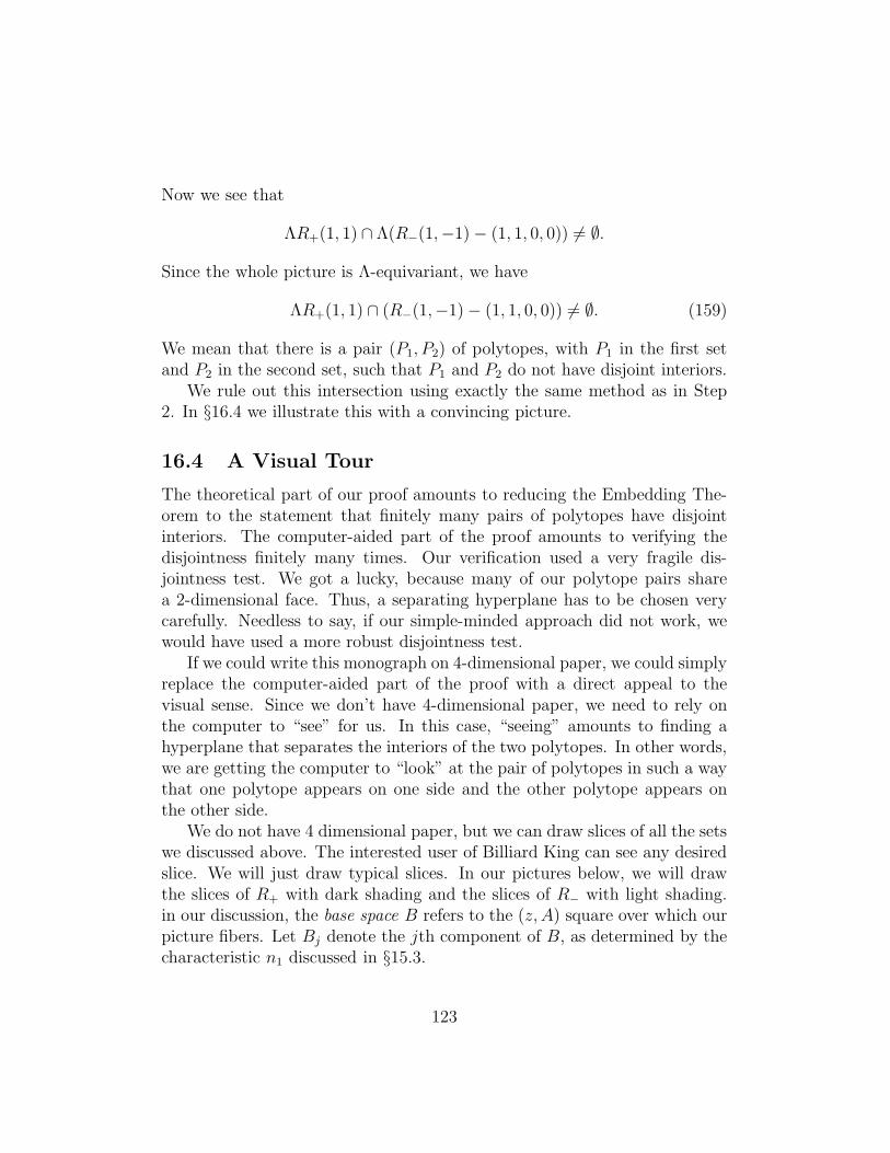
Now we see that

ΛR+(1, 1) ∩ Λ(R−(1,−1)− (1, 1, 0, 0)) 6= ∅.

Since the whole picture is Λ-equivariant, we have

ΛR+(1, 1) ∩ (R−(1,−1)− (1, 1, 0, 0)) 6= ∅. (159)

We mean that there is a pair (P1, P2) of polytopes, with P1 in the first setand P2 in the second set, such that P1 and P2 do not have disjoint interiors.

We rule out this intersection using exactly the same method as in Step2. In §16.4 we illustrate this with a convincing picture.

16.4 A Visual Tour

The theoretical part of our proof amounts to reducing the Embedding The-orem to the statement that finitely many pairs of polytopes have disjointinteriors. The computer-aided part of the proof amounts to verifying thedisjointness finitely many times. Our verification used a very fragile dis-jointness test. We got a lucky, because many of our polytope pairs sharea 2-dimensional face. Thus, a separating hyperplane has to be chosen verycarefully. Needless to say, if our simple-minded approach did not work, wewould have used a more robust disjointness test.

If we could write this monograph on 4-dimensional paper, we could simplyreplace the computer-aided part of the proof with a direct appeal to thevisual sense. Since we don’t have 4-dimensional paper, we need to rely onthe computer to “see” for us. In this case, “seeing” amounts to finding ahyperplane that separates the interiors of the two polytopes. In other words,we are getting the computer to “look” at the pair of polytopes in such a waythat one polytope appears on one side and the other polytope appears onthe other side.

We do not have 4 dimensional paper, but we can draw slices of all the setswe discussed above. The interested user of Billiard King can see any desiredslice. We will just draw typical slices. In our pictures below, we will drawthe slices of R+ with dark shading and the slices of R− with light shading.in our discussion, the base space B refers to the (z, A) square over which ourpicture fibers. Let Bj denote the jth component of B, as determined by thecharacteristic n1 discussed in §15.3.

123

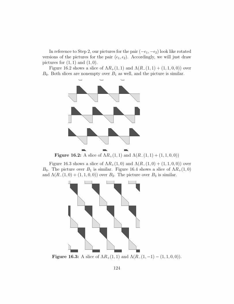
In reference to Step 2, our pictures for the pair (−ǫ1,−ǫ2) look like rotatedversions of the pictures for the pair (ǫ1, ǫ2). Accordingly, we will just drawpictures for (1, 1) and (1, 0).

Figure 16.2 shows a slice of ΛR+(1, 1) and Λ(R−(1, 1) + (1, 1, 0, 0)) overB0. Both slices are nonempty over B1 as well, and the picture is similar.

Figure 16.2: A slice of ΛR+(1, 1) and Λ(R−(1, 1) + (1, 1, 0, 0))

Figure 16.3 shows a slice of ΛR+(1, 0) and Λ(R−(1, 0) + (1, 1, 0, 0)) overB0. The picture over B1 is similar. Figure 16.4 shows a slice of ΛR+(1, 0)and Λ(R−(1, 0) + (1, 1, 0, 0)) over B2. The picture over B3 is similar.

Figure 16.3: A slice of ΛR+(1, 1) and Λ(R−(1,−1)− (1, 1, 0, 0)).

124

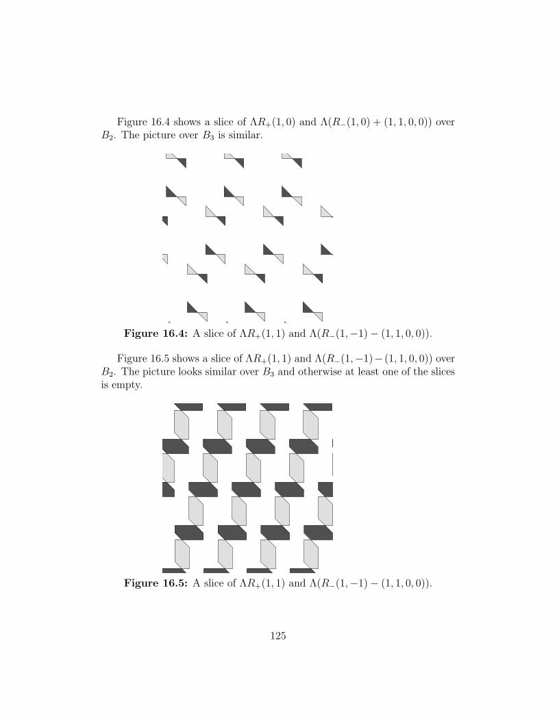
Figure 16.4 shows a slice of ΛR+(1, 0) and Λ(R−(1, 0) + (1, 1, 0, 0)) overB2. The picture over B3 is similar.

Figure 16.4: A slice of ΛR+(1, 1) and Λ(R−(1,−1)− (1, 1, 0, 0)).

Figure 16.5 shows a slice of ΛR+(1, 1) and Λ(R−(1,−1)− (1, 1, 0, 0)) overB2. The picture looks similar over B3 and otherwise at least one of the slicesis empty.

Figure 16.5: A slice of ΛR+(1, 1) and Λ(R−(1,−1)− (1, 1, 0, 0)).

125

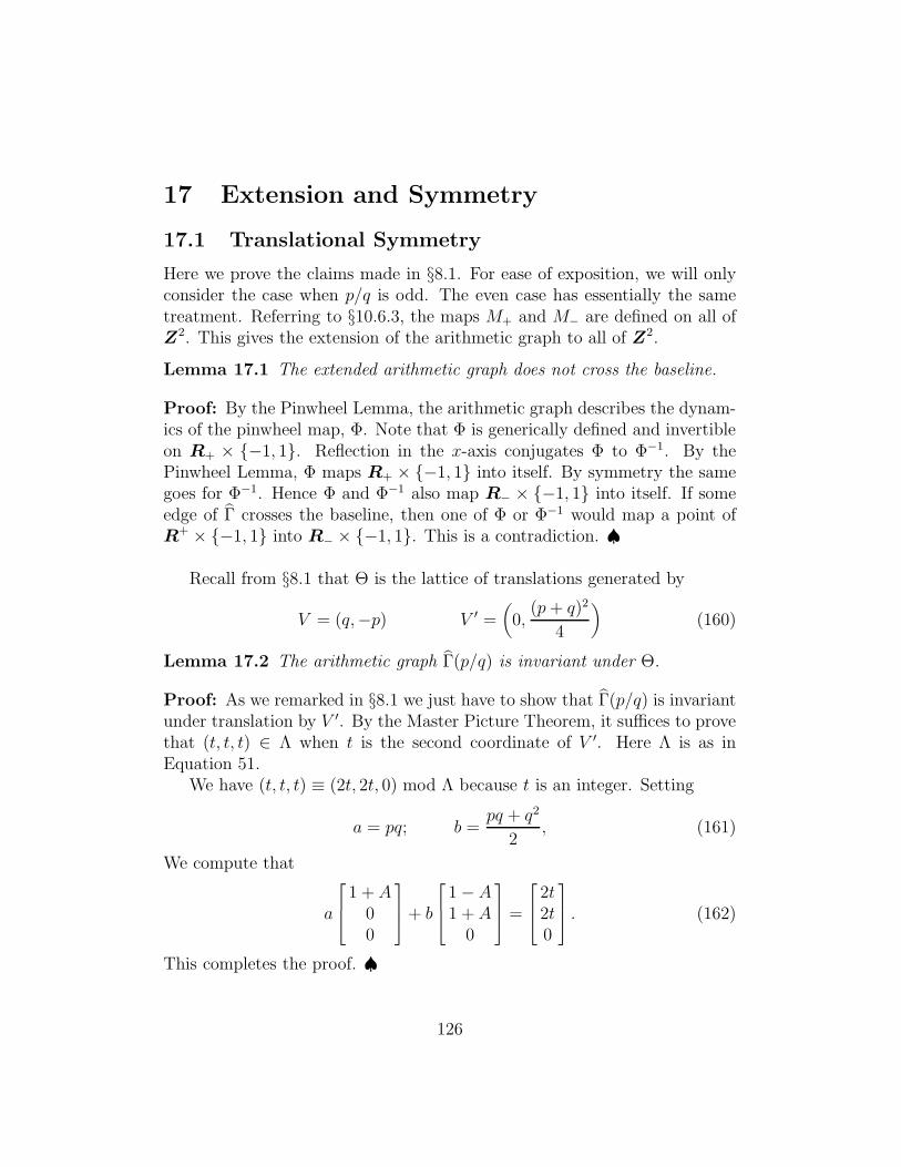
17 Extension and Symmetry

17.1 Translational Symmetry

Here we prove the claims made in §8.1. For ease of exposition, we will onlyconsider the case when p/q is odd. The even case has essentially the sametreatment. Referring to §10.6.3, the maps M+ and M− are defined on all ofZ2. This gives the extension of the arithmetic graph to all of Z2.

Lemma 17.1 The extended arithmetic graph does not cross the baseline.

Proof: By the Pinwheel Lemma, the arithmetic graph describes the dynam-ics of the pinwheel map, Φ. Note that Φ is generically defined and invertibleon R+ × {−1, 1}. Reflection in the x-axis conjugates Φ to Φ−1. By thePinwheel Lemma, Φ maps R+ × {−1, 1} into itself. By symmetry the samegoes for Φ−1. Hence Φ and Φ−1 also map R− × {−1, 1} into itself. If someedge of Γ crosses the baseline, then one of Φ or Φ−1 would map a point ofR+ × {−1, 1} into R− × {−1, 1}. This is a contradiction. ♠

Recall from §8.1 that Θ is the lattice of translations generated by

V = (q,−p) V ′ =(0,

(p+ q)2

4

)(160)

Lemma 17.2 The arithmetic graph Γ(p/q) is invariant under Θ.

Proof: As we remarked in §8.1 we just have to show that Γ(p/q) is invariantunder translation by V ′. By the Master Picture Theorem, it suffices to provethat (t, t, t) ∈ Λ when t is the second coordinate of V ′. Here Λ is as inEquation 51.

We have (t, t, t) ≡ (2t, 2t, 0) mod Λ because t is an integer. Setting

a = pq; b =pq + q2

2, (161)

We compute that

a

1 + A00

+ b

1− A1 + A

0

=

2t2t0

. (162)

This completes the proof. ♠

126

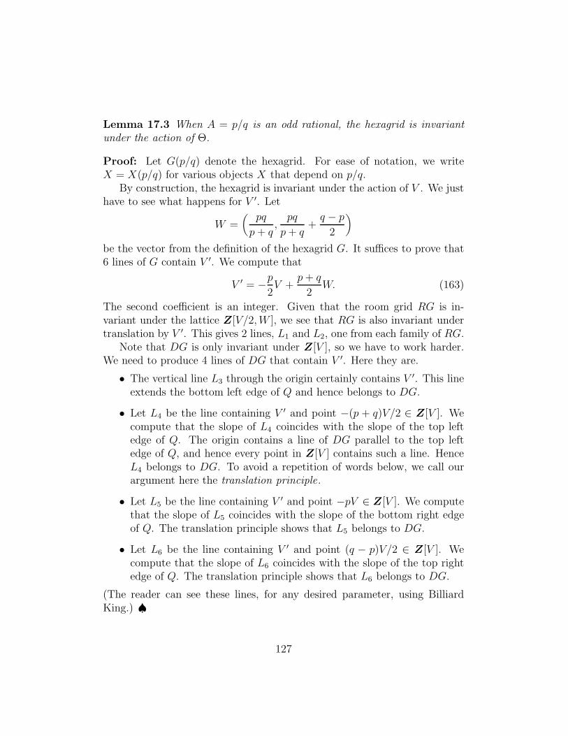
Lemma 17.3 When A = p/q is an odd rational, the hexagrid is invariantunder the action of Θ.

Proof: Let G(p/q) denote the hexagrid. For ease of notation, we writeX = X(p/q) for various objects X that depend on p/q.

By construction, the hexagrid is invariant under the action of V . We justhave to see what happens for V ′. Let

W =(

pq

p+ q,pq

p+ q+q − p

2

)

be the vector from the definition of the hexagrid G. It suffices to prove that6 lines of G contain V ′. We compute that

V ′ = −p2V +

p+ q

2W. (163)

The second coefficient is an integer. Given that the room grid RG is in-variant under the lattice Z[V/2,W ], we see that RG is also invariant undertranslation by V ′. This gives 2 lines, L1 and L2, one from each family of RG.

Note that DG is only invariant under Z[V ], so we have to work harder.We need to produce 4 lines of DG that contain V ′. Here they are.

• The vertical line L3 through the origin certainly contains V ′. This lineextends the bottom left edge of Q and hence belongs to DG.

• Let L4 be the line containing V ′ and point −(p + q)V/2 ∈ Z[V ]. Wecompute that the slope of L4 coincides with the slope of the top leftedge of Q. The origin contains a line of DG parallel to the top leftedge of Q, and hence every point in Z[V ] contains such a line. HenceL4 belongs to DG. To avoid a repetition of words below, we call ourargument here the translation principle.

• Let L5 be the line containing V ′ and point −pV ∈ Z[V ]. We computethat the slope of L5 coincides with the slope of the bottom right edgeof Q. The translation principle shows that L5 belongs to DG.

• Let L6 be the line containing V ′ and point (q − p)V/2 ∈ Z[V ]. Wecompute that the slope of L6 coincides with the slope of the top rightedge of Q. The translation principle shows that L6 belongs to DG.

(The reader can see these lines, for any desired parameter, using BilliardKing.) ♠

127

17.2 Rotational Symmetry

Here we will establish the rotational symmetry of the arithmetic graph thatwe discussed in §8.2. Again, we assume that p/q is odd. (We didn’t discussrotational symmetry in the even case.) Let p+/q+ be as in §8.2. Let ι denote180 degree rotation about the point (q+,−p+)/2. We have

ι(m,n) = (q+, p−+)− (m,n). (164)

Here is the main result of this section.

Lemma 17.4 ι(Γ) = Γ.

Proof: Let M+ and M− be as in §10.6.3. As usual, we take α = 1/(2q). Wewill first compare M+(m,n) with M−(ι(m,n)). We have

M+(m,n) = (t, t+ 1, t) mod Λ;pm

q+ n+

1

2q(165)

Next, we haveM−(ι(m,n)) = (t′ − 1, t′, t′) mod Λ;

t′ =(ap

q− b

)−

(pm

q+ n

)+

1

2q=

(ap− bq

q

)−

(pm

q+ n

)+

1

2q=

−1

q−

(pm

q+ n

)+

1

2q= −

(pm

q+ n

)− 1

2q= −t.

In shortM−(ι(m,n)) = (−t− 1,−t,−t) mod Λ. (166)

Recall that RA is the fundamental domain for the action of Λ = ΛA. Wemean to equate Λ with the Z span of its columns. There is some v ∈ Λ suchthat

(s1, s2, s3) = (t, t+ 1, t) + (v1, v2, v3) ∈ RA (167)

Given Equation 51, we have (2 +A,A, 1) ∈ Λ. Hence

w = (−v1 + 2 + A,−v2 + A,−v3 + 1) ∈ Λ. (168)

128

We compute that

(−t− 1,−t,−t) + w = (1 + A, 1 + A, 1)− (s1, s2, s3). (169)

So, we haveM+(m,n) = ρ ◦M−(ι(m,n)), (170)

where ρ is reflection through the midpoint of the space RA. A similar calcu-lation shows

M−(m,n) = ρ ◦M+(ι(m,n)), (171)

But now we just verify by inspection that our partition of RA is symmetricunder ρ, and has the labels appropriate to force the type determined by

ρ ◦M+(m,n), ρ ◦M−(m,n)

to be the 180 degree rotation of the type forced by

M−(m,n), M+(m,n)

Indeed, we can determine this with an experiment performed on any rationallarge enough such that all regions are sampled. A little inspection of thepicture of Γ(3/7), for instance, suffices to finish the proof. Compare Figure3.6. ♠

Since Γ is also invariant under the lattice Θ of translations, we see thatthere are actually infinitely many points of order 2 symmetry.

129

18 The Structure of the Doors

18.1 The Odd Case

We suppose that p/q is an odd rational. Say that a wall line is a line ofpositive slope in the room grid. The doors are the intersection points of linesin the door grid with the wall lines. Let L0 be the wall line through (0, 0).Let L1 be the wall line through V/2.

Lemma 18.1 Any two wall lines are equivalent mod Θ.

Proof: We check explicitly that the vector

V ′ +p + 1

2V ∈ Θ ∩ L1

Hence L0 and L1 are equivalent mod Θ. But any other wall line is obtainedfrom one of L0 or L1 by adding a suitable integer multiple of V . ♠

Lemma 18.2 The first coordinate of any door is an integer.

Proof: Any wall line is equivalent mod Θ to L0. Since Θ acts by integertranslations, it suffices to door lies on L0. Such a door is an integer multipleof the point v3 in Figure 4.1. That is, our door has coordinates

k

2q(2pq, (p+ q)2 − 2p2). (172)

The first coordinate here is certainly an integer. ♠

It could happen that the second coordinate of a door is an integer. Callsuch a door exceptional.

Lemma 18.3 Modulo the action of Θ, there are only two exceptional doors.

Proof: The point (0, 0) gives rise to two exceptional doors with (the same)integer coordinates. One of these doors is associated to the wall above (0, 0),and one of these doors is associated to the door below. Hence, it suffices toshow that any door with integer coordinates lies in Θ.

130

As in the preceding result, it suffices to consider doors on L0. GivenEquation 172, we see that

k(p+ q)2 − 2p2

2q∈ Z

for an exceptional door. Expanding this out, and observing that q dividesboth q2 and pq, we get that

kq2 − p2

2q∈ Z.

But q and q2 − p2 are relatively prime. Hence k = jq for some j ∈ Z. But

qv3 = 2V ′ + V ∈ Θ.

Hence jqv3 = kv3 ∈ Θ as well. ♠

Here is a related result.

Lemma 18.4 Any lattice point on a wall line is equivalent to (0, 0) mod Θ.

Proof: By symmetry, it suffices to consider the cases when (m,n) ∈ L0.Looking at Figure 4.1, we see that any point on L0 has the form

sv5 =s

2(p+ q)(2pq, (p+ q)2 − 2p2). (173)

In order for this point to lie in Z2, the first coordinate must be an integer.Since p and q are relatively prime, pq and p+ q are relatively prime. Hence,the first coordinate is an integer only if s = k(p+ q) for some k ∈ Z. Hence(m,n) is an integer multiple of the point

(p+ q)v5 =(pq,

(p+ q)2

2− p2

)= 2V ′ + pV ∈ Θ.

Here V and V ′ are the vectors generating Θ, as in Equation 160. ♠

The vertical lines in the door grid have the form x = kq for k ∈ Z. Saythat a Type 1 door is the intersection of such a line with a wall line.

131

Lemma 18.5 Let (kq, y) be a Type 1 door. Then py ∈ Z.

Proof: The group Θ acts transitively, by integer translations, on the verticallines of the door grid. Hence, is suffices to prove this lemma for the case k = 0.In other words, we need to show that py ∈ Z if (0, y) lies on a wall line.

We order the wall lines according to the order in which they intersect theline of slope −A = −p/q through the origin. Let yn be such that (0, yn) lieson the kth wall line. The sequence {yn} is an arithmetic progression. Hence,it suffices to prove our result for two consecutive values of n. Note that (0, 0)is a type A door. We might as well normalize so that y0 = 0. Then (0, y1)lies on the wall line L1 through (−q, p). Referring to Equation 12, two pointson L1 are −V and −V +W . These points are given by

−V = (−q, p); −VW = (−q, p) +(

pq

p+ q,pq

p+ q+q − p

2

).

From this information, we compute that y1 = (p+q)2/2p. Since p+q is even,py1 = (p+ q)2/2 ∈ Z. ♠

Recall that y is the greatest integer less than y.

Corollary 18.6 Suppose that (x, y) is a door of type 1, then y − y 6= 1/2.

Proof: p(y − y) = p/2 is an integer, by the previous result. But p/2 is notan integer. This is a contradiction. ♠

Say that a Type 2 door is a door on L0 that is not of Type 1. One obtainsa Type 2 door by intersecting L0 with a line of the door grid that is parallelto the top left (or right) edge of the arithmetic kite.

Lemma 18.7 The Type 2 doors are precisely the points on L0 of the form(kp, yk), where k ∈ Z and yk is a number that depends on k.

Proof: Referring to Figure 4.1, two consecutive doors on L0 are (0, 0) andv3 = (p, y1). Our lemma now follows from the fact that the sequence of doorson L0 forms an arithmetic progression. ♠

132

18.2 The Even Case

Now we revisit all the results above in case p/q is even.

Lemma 18.8 Any two wall lines are equivalent mod Θ.

Proof: This is easy in the even case. Translation by V maps each wall lineto the adjacent one. ♠

Lemma 18.9 The first coordinate of any door is an integer.

Proof: The first door on L0 is the same in the even case as in the odd case.The rest of the proof is the same as in the odd case. ♠

Lemma 18.10 Modulo the action of Θ, there are only two exceptional doors.

Proof: As in the odd case, we just have to show that any door with integercoordinates is equivalent to (0, 0) mod Θ. As in the odd case, the doors onL0 have the form kv3. As in the odd case, this leads to the statement that

kq2 − p2

2q∈ Z.

Now the proof is a bit different. Here 2q and q2 − p2 are relatively prime.Hence k = 2jq for some j ∈ Z. But

2qv3 = V ′ + 2V ∈ Θ.

Hence 2jqv3 = kv3 ∈ Θ as well. ♠

Lemma 18.11 Any lattice point on a wall line is equivalent to (0, 0) modΘ.

133

Proof: As in the proof of Lemma 18.4, we see that

sv5 =s

2(p+ q)(2pq, (p+ q)2 − 2p2) ∈ Z. (174)

As in the odd case, we look at the first coordinate and deduce the fact thats = k(p + q) for some k ∈ Z. This is not enough for us in the even case.Looking now at the second coordinate, we see that

k(p+ q)

2− kp2 ∈ Z.

Hence k is even. Hence (m,n) is an integer multiple of the point

2(p+ q)v5 = (2pq, (p+ q)2 − 2p2) = V ′ + 2pV ∈ Θ.

♠

We don’t repeat the proof of Lemma 18.5 because we don’t need it. Weonly need the even version of Corollary 18.6. In the even case, we have simplyforced Corollary 18.6 to be true by eliminating the crossings for which it fails.

We say that a Type 2 door is a door on L0 that is not of Type 1, and also isnot one of the crossings we have eliminated. Once we make this redefinition,we have the following result

Lemma 18.12 The Type 2 doors are precisely the points on L0 of the form(kp, yk), where k ∈ Z is not an odd multiple of q, and yk is a number thatdepends on k.

Proof: The Type two doors are as in the odd case, except that we eliminatethe points (kp, yk) where k is an odd multiple of q. ♠

134

19 Proof of the Hexagrid Theorem I

19.1 The Key Result

We will assume that p/q is an odd rational until the end of the chapter.Say that a floor line is a negatively sloped line of the floor grid. Say that

a floor point is a point on a floor line. Such a point need not have integercoordinates. Let M+ and M− denote the maps from Equation 10.6.3.

Lemma 19.1 If (m,n) is a floor point, then M−(m,n) is equivalent mod Λto a point of the form (β, 0, 0).

Proof: The map M− is constant when restricted to each floor line, becausethese lines have slope −A. Hence, it suffices to prove this result for one pointon each floor line. The points

(0, t); t =k(p+ q)

2; k ∈ Z. (175)

form a sequence of floor points, one per floor line. Note that t is an integer,because p+ q is even.

To compute the image of the point (0, t), we just have to subject the pointt to our reduction algorithm from §15.2. The first 4 steps of the algorithmlead to the following result.

1. z = t.

2. Z = floor(t) = t, because t is an integer.

3. y = 2t = k(p+ q) = kq(1 + A).

4. Y = floor(y/(1 + A)) = kq.

Hence z = Z and y = (1 + A)Y . Hence

M−(0, t) = (x− (1 + A)X, y − (1 + A)Y, z − Z) = (β, 0, 0), (176)

for some number β ∈ R that depends on A and k. ♠

135

19.2 Two Special Planes

Let Π− ⊂ R3 denote the plane given by y = z. We can think of Π− as theplane through the origin generated by the vectors (1, 0, 0) and (1, 1, 1). Inparticular, the vector (1, 1, 1) is contained in Π−. Let Π−(0) denote the linethrough the origin parallel to (1, 0, 0). Then Π−(0) is a line in Π−. Define

Π+ = Π− + (1, 1, 0); Π+(0) = Π−(0) + (1, 1, 0). (177)

Lemma 19.2 If (m,n) is a floor point, then M±(m,n) is equivalent mod Λto a point in Π±(0).

Proof: The (−) case of this result is just a restatement of Lemma 19.1. The(+) case follows from the (−) case and symmetry. That is, we just translatethe (−) case by the vector (1, 1, 0) to get the (+) case. ♠

DefineΠ±(r) = Π±(0) + (r, r, r). (178)

Let Π±(r, s) denote the open infinite strip that is bounded by Π±(r) andΠ±(s). In the case of interest to us, we will have r = 0 and s = λ > 0.

For each pair (ǫ1, ǫ2) ∈ {−1, 0, 1}2, let Σ(ǫ1, ǫ2) denote the set of latticepoints (m,n) such that (m,n) and (m,n) + (ǫ1, ǫ2) are separated by somefloor line. The set Σ(ǫ1, ǫ2) is obtained by intersecting Z2 with an infiniteunion of evenly spaced infinite strips, each of which has a floor line as oneboundary component. For our purposes, it suffices to consider the pairs

(−1, 0); (−1,−1); (0,−1); (1,−1). (179)

For these pairs, the floor lines are the lower boundaries of the strips. Wedefine

λ(ǫ1, ǫ2) = −(Aǫ1 + ǫ2). (180)

Lemma 19.3 Let λ = λ(ǫ1, ǫ2). Suppose that (m,n) ∈ Σ(ǫ1, ǫ2). ThenM±(m,n) ∈ Π±(0, λ).

Proof: We consider the case of M− and the pair (−1, 0). The other caseshave essentially the same proof. If (m,n) ∈ Σ(−1, 0), Then there is somex ∈ (m − 1, m) such that (x, n) is a floor point. Then M+(x, n) is Λ-equivalent to a point p in Π(0). But then M+(m,n) is Λ-equivalent top+ (m− x)(A,A,A) ∈ Π(0, A) = Π(0, λ(−1, 0)). ♠

136

19.3 Critical Points

Say that a point v ∈ Σ(ǫ1, ǫ2) is critical for (ǫ1, ǫ2) if the arithmetic graphcontains the edge joining (m,n) to (m + ǫ1, n + ǫ2). Statement 1 of theHexagrid Theorem says, in particular, that there are no such points like this.

Lemma 19.4 There are no critical points.

Proof: LetR+ denote the tiling of R3 by polyhedra, according to the MasterPicture Theorem. Let P+ denote the intersection of R+ with the plane Π.We make the same definitions in the (−) case. If (m,n) is critical for (ǫ1, ǫ2),then one of two things is true.

1. Π+(0, λ) nontrivially intersects a polygon of P+ labelled by (ǫ1, ǫ2).

2. Π−(0, λ) nontrivially intersects a polygon of P− labelled by (ǫ1, ǫ2).

Here we have set λ = λ(ǫ1, ǫ2). Considering the 4 pairs of interest to us, andthe 2 possible signs, we have 8 conditions to rule out. We check, in all cases,that the relevant strip is disjoint from the relevant polygons.

We can check the disjointness for all parameters at once. The union

S±(ǫ1, ǫ2) :=⋃

A∈(0,1)

(Π±(ǫ1, ǫ2;A)× {A}

)

is a polyhedral subset of R4. To get an honest polyhedron, we observe thatS is invariant the action of the lattice element γ1 from Equation 55, and wetake a polyhedron whose union under translates by γ3 tiles S. In practice,we simply restrict the x-coordinate to lie in [0, 2].

We check that S±(ǫ1, ǫ2), or rather the compact polyhedron replacing it,is disjoint from all Λ-translates of the polytope P±(ǫ1, ǫ2), the polytope listedin §15.3. In practice, most translates are very far away, and we only need tocheck a small finite list. This is a purely algebraic calculation. ♠

Rather than dwell on the disjointness calculation, which gives no insightinto what is going on, we will draw pictures for the parameter A = 1/3. Thecombinatorial type changes with the parameter, but not the basic features ofinterest to us. The interested reader can see the pictures for any parameterusing Billiard King.

137

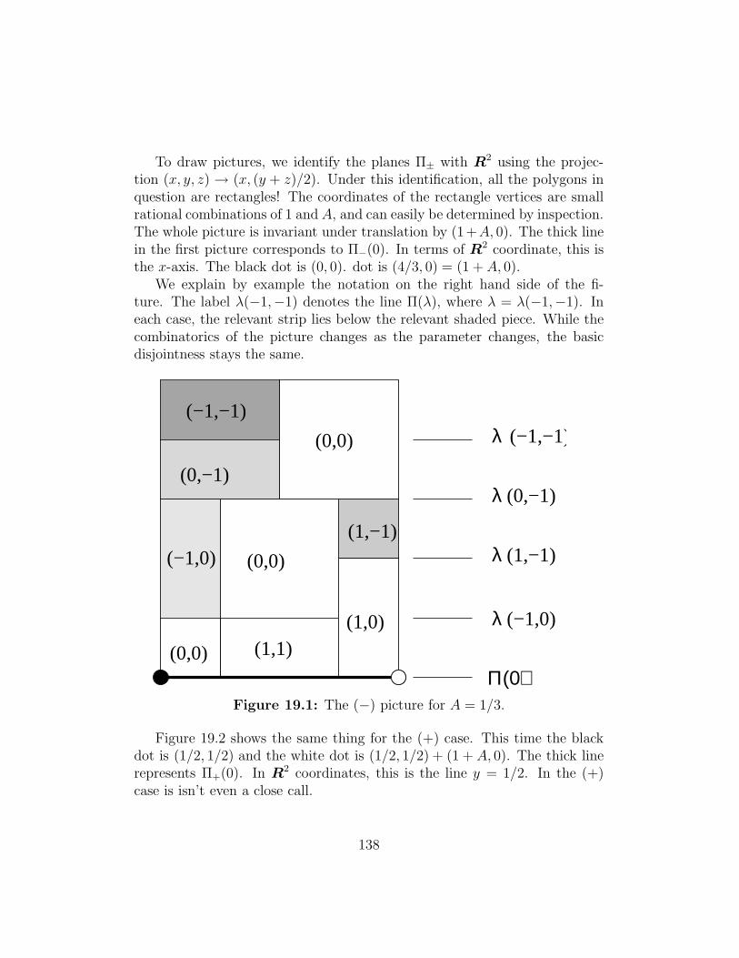
To draw pictures, we identify the planes Π± with R2 using the projec-tion (x, y, z) → (x, (y + z)/2). Under this identification, all the polygons inquestion are rectangles! The coordinates of the rectangle vertices are smallrational combinations of 1 and A, and can easily be determined by inspection.The whole picture is invariant under translation by (1+A, 0). The thick linein the first picture corresponds to Π−(0). In terms of R2 coordinate, this isthe x-axis. The black dot is (0, 0). dot is (4/3, 0) = (1 +A, 0).

We explain by example the notation on the right hand side of the fi-ture. The label λ(−1,−1) denotes the line Π(λ), where λ = λ(−1,−1). Ineach case, the relevant strip lies below the relevant shaded piece. While thecombinatorics of the picture changes as the parameter changes, the basicdisjointness stays the same.

(0,−1)

λ (−1,−1)

λ (−1,0)

λ (1,−1)

λ

Π(0)

(1,−1)(−1,0) (0,0)

(0,0)

(0,0) (1,1)(1,0)

(0,−1)

(−1,−1)

Figure 19.1: The (−) picture for A = 1/3.

Figure 19.2 shows the same thing for the (+) case. This time the blackdot is (1/2, 1/2) and the white dot is (1/2, 1/2) + (1 + A, 0). The thick linerepresents Π+(0). In R2 coordinates, this is the line y = 1/2. In the (+)case is isn’t even a close call.

138

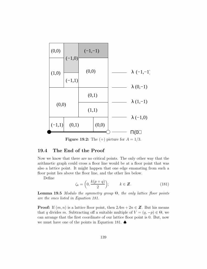
λ (−1,−1)

λ (−1,0)

λ (1,−1)

λ (0,−1)

Π(0)

(−1,0)

(0,0)(0,1)(−1,1)

(0,0)(1,1)

(0,1)

(0,0)

(−1,1)

(−1,−1)(0,0)

(1,0)

Figure 19.2: The (+) picture for A = 1/3.

19.4 The End of the Proof

Now we know that there are no critical points. The only other way that thearithmetic graph could cross a floor line would be at a floor point that wasalso a lattice point. It might happen that one edge emanating from such afloor point lies above the floor line, and the other lies below.

Define

ζk =(0,k(p + q)

2

); k ∈ Z. (181)

Lemma 19.5 Modulo the symmetry group Θ, the only lattice floor pointsare the ones listed in Equation 181.

Proof: If (m,n) is a lattice floor point, then 2Am+ 2n ∈ Z. But his meansthat q divides m. Subtracting off a suitable multiple of V = (q,−p) ∈ Θ, wecan arrange that the first coordinate of our lattice floor point is 0. But, nowwe must have one of the points in Equation 181. ♠

139

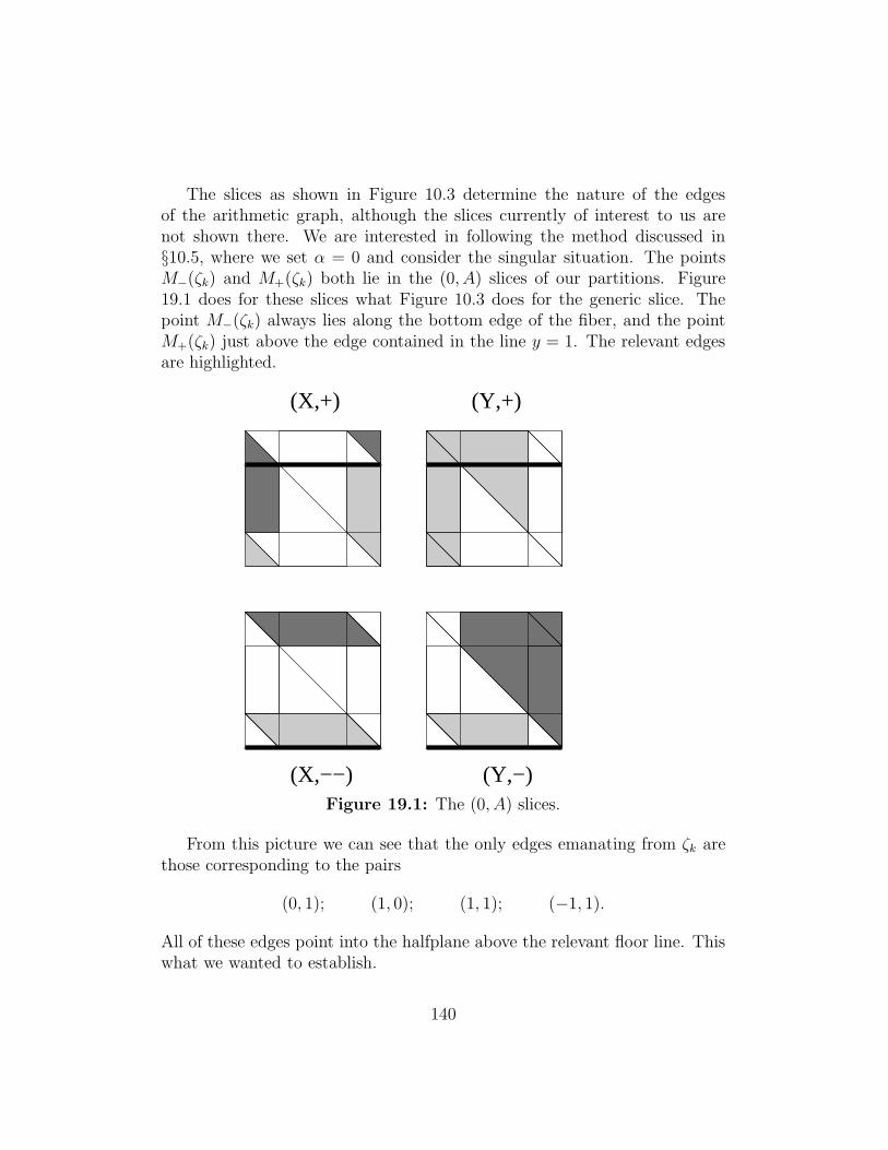
The slices as shown in Figure 10.3 determine the nature of the edgesof the arithmetic graph, although the slices currently of interest to us arenot shown there. We are interested in following the method discussed in§10.5, where we set α = 0 and consider the singular situation. The pointsM−(ζk) and M+(ζk) both lie in the (0, A) slices of our partitions. Figure19.1 does for these slices what Figure 10.3 does for the generic slice. Thepoint M−(ζk) always lies along the bottom edge of the fiber, and the pointM+(ζk) just above the edge contained in the line y = 1. The relevant edgesare highlighted.

(Y,−)

(Y,+)(X,+)

(X,−−)Figure 19.1: The (0, A) slices.

From this picture we can see that the only edges emanating from ζk arethose corresponding to the pairs

(0, 1); (1, 0); (1, 1); (−1, 1).

All of these edges point into the halfplane above the relevant floor line. Thiswhat we wanted to establish.

140

19.5 The Even Case

The only place where we used the fact that p/q is odd was in Lemma 19.1.We needed to know that the number t in Equation 19.1 was odd. This nolonger works when p + q is odd. However, when p/q is even, the floor gridhas a different definition: Only the even floor lines are present in the grid.That is, the number k in Equation 19.1 is an even integer. Hence, for thefloor lines in the even case, the number t is an integer. The rest of the proofof Lemma 19.1 works word for word. The rest of the proof of Statement 1goes through word for word.

141

20 Proof of the Hexagrid Theorem II

20.1 The Basic Definitions

As in the previous chapter, we will take p/q odd until the very end. It turnsout that the secret to proving Statement 2 of the Hexagrid Theorem is touse variants of the maps M+ and M− from Equation 10.6.3. Let A ∈ (0, 1)be any parameter. Let Λ the lattice from the Master Picture Theorem. LetΠ ⊂ R3 be the plane defined by the relation x+ y = A.

For (m,n) ∈ R2 we define ∆+(m,n) = (x, y, z), where

x = 2A(1−m+ n)−m; y = A− x; z = Am. (182)

We also define∆−(m,n) = ∆+(m,n) + (−A,A, 0). (183)

Note that ∆±(m,n) ∈ Π. Indeed, ∆ is an affine isomorphism from R2 ontoΠ.

Lemma 20.1 Suppose that (m,n) ∈ Z2. Then ∆±(m,n) and M±(m,n) areequivalent mod Λ.

Proof: Let v1, v2, v3 be the three columns of the matrix defining Λ. So,v1 = (1 + A, 0, 0) and v1 = (1− A, 1 + A, 0) and v3 = (−1,−1, 1). Let

c1 = −1 + 2m; c2 = 1−m+ 2n; c3 = n.

We compute directly that

M+(m,n)−∆+(m,n) = c1v1 + c2v2 + c3v3.

M−(m,n)−∆−(m,n) = c1v1 + (c2 − 1)v2 + c3v3.

This completes the proof. ♠

We introduce the vector

ζ = (−A,A, 1) ∈ Λ. (184)

Referring to the proof of our last result, we have ζ = v2 + v3. This explainswhy ζ ∈ Λ. Note that Π is invariant under translation by ζ .

142

20.2 Interaction with the Hexagrid

Now we will specialize to the case when A = p/q is an odd rational. Theresults above hold, and we can also define the hexagrid. We will see how themaps ∆+ and ∆− interact with the Hexagrid. Let L0 denote the wall linethrough the origin.

Lemma 20.2 ∆±(L0) is parallel to ζ and contains (−2A,A, 0).

Proof: We refer to the points in Figure 4.1. The points v5 and v1 both lieon L0. We compute

∆+(v5)−∆+(v1) =p2

p + qζ.

Hence ∆+(L0) is parallel to ζ . We compute that ∆+(0, 0) = (2A,−A, 0). ♠

We introduce the notation Π(x) to denote the line in Π that is parallelto ζ and contains the point (x,A− x, 0). For instance,

∆+(0, 0) ⊂ Π(2A); ∆−(0, 0) ⊂ Π(A). (185)

Let Π(r, s) denote the infinite strip bounded by the lines Π(r) and Π(s).For each pair of indices (ǫ1, ǫ2) ∈ {−1, 0, 1}2, we let Σ(ǫ1, ǫ2) denote the

set of lattice points (m,n) such that L0 separates (m,n) from (m+ǫ1, n+ǫ2).Now we define constants

λ(0, 1) = 2A λ(−1,−1) = 1−A2;

λ(−1, 0) = 1 + 2A− A2 λ(−1, 1) = 1 + 4A− A2 (186)

Lemma 20.3 Let (ǫ1, ǫ2) be any of the 4 pairs listed above. Let λ = λ(ǫ1, ǫ2).The following 3 statements are equivalent.

1. (m,n) ∈ Σ(ǫ1, ǫ2).

2. ∆+(m,n) is congruent mod Λ to a point in the interior of Π(2A−λ, 2A).

3. ∆−(m,n) is congruent mod Λ to a point in the interior of Π(A−λ,A).

143

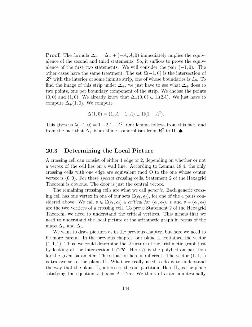
Proof: The formula ∆− = ∆+ + (−A,A, 0) immediately implies the equiv-alence of the second and third statements. So, it suffices to prove the equiv-alence of the first two statements. We will consider the pair (−1, 0). Theother cases have the same treatment. The set Σ(−1, 0) is the intersection ofZ2 with the interior of some infinite strip, one of whose boundaries is L0. Tofind the image of this strip under ∆+, we just have to see what ∆+ does totwo points, one per boundary component of the strip. We choose the points(0, 0) and (1, 0). We already know that ∆+(0, 0) ⊂ Π(2A). We just have tocompute ∆+(1, 0). We compute

∆(1, 0) = (1, A− 1, A) ⊂ Π(1−A2).

This gives us λ(−1, 0) = 1+2A−A2. Our lemma follows from this fact, andfrom the fact that ∆+ is an affine isomorphism from R2 to Π. ♠

20.3 Determining the Local Picture

A crossing cell can consist of either 1 edge or 2, depending on whether or nota vertex of the cell lies on a wall line. According to Lemma 18.4, the onlycrossing cells with one edge are equivalent mod Θ to the one whose centervertex is (0, 0). For these special crossing cells, Statement 2 of the HexagridTheorem is obvious. The door is just the central vertex.

The remaining crossing cells are what we call generic. Each generic cross-ing cell has one vertex in one of our sets Σ(ǫ1, ǫ2), for one of the 4 pairs con-sidered above. We call v ∈ Σ(ǫ1, ǫ2) a critical for (ǫ1, ǫ2). v and v + (ǫ1, ǫ2)are the two vertices of a crossing cell. To prove Statement 2 of the HexagridTheorem, we need to understand the critical vertices. This means that weneed to understand the local picture of the arithmetic graph in terms of themaps ∆+ and ∆−.

We want to draw pictures as in the previous chapter, but here we need tobe more careful. In the previous chapter, our plane Π contained the vector(1, 1, 1). Thus, we could determine the structure of the arithmetic graph justby looking at the intersection Π ∩ R. Here R is the polyhedron partitionfor the given parameter. The situation here is different. The vector (1, 1, 1)is transverse to the plane Π. What we really need to do is to understandthe way that the plane Πα intersects the our partition. Here Πα is the planesatisfying the equation x + y = A + 2α. We think of α an infinitesimally

144

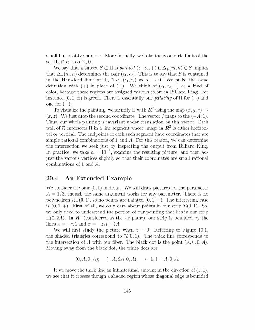
small but positive number. More formally, we take the geometric limit of theset Πα ∩R as αց 0.

We say that a subset S ⊂ Π is painted (ǫ1, ǫ2,+) if ∆+(m,n) ∈ S impliesthat ∆+(m,n) determines the pair (ǫ1, ǫ2). This is to say that S is containedin the Hausdorff limit of Πα ∩ R+(ǫ1, ǫ2) as α → 0. We make the samedefinition with (+) in place of (−). We think of (ǫ1, ǫ2,±) as a kind ofcolor, because these regions are assigned various colors in Billiard King. Forinstance (0, 1,±) is green. There is essentially one painting of Π for (+) andone for (−).

To visualize the painting, we identify Π with R2 using the map (x, y, z)→(x, z). We just drop the second coordinate. The vector ζ maps to the (−A, 1).Thus, our whole painting is invariant under translation by this vector. Eachwall of R intersects Π in a line segment whose image in R2 is either horizon-tal or vertical. The endpoints of each such segment have coordinates that aresimple rational combinations of 1 and A. For this reason, we can determinethe intersection we seek just by inspecting the output from Billiard King.In practice, we take α = 10−5, examine the resulting picture, and then ad-just the various vertices slightly so that their coordinates are small rationalcombinations of 1 and A.

20.4 An Extended Example

We consider the pair (0, 1) in detail. We will draw pictures for the parameterA = 1/3, though the same argument works for any parameter. There is nopolyhedron R−(0, 1), so no points are painted (0, 1,−). The interesting caseis (0, 1,+). First of all, we only care about points in our strip Σ(0, 1). So,we only need to understand the portion of our painting that lies in our stripΠ(0, 2A). In R2 (considered as the xz plane), our strip is bounded by thelines x = −zA and x = −zA + 2A.

We will first study the picture when z = 0. Referring to Figure 19.1,the shaded triangles correspond to R(0, 1). The thick line corresponds tothe intersection of Π with our fiber. The black dot is the point (A, 0, 0, A).Moving away from the black dot, the white dots are

(0, A, 0, A); (−A, 2A, 0, A); (−1, 1 + A, 0, A.

It we move the thick line an infinitesimal amount in the direction of (1, 1),we see that it crosses though a shaded region whose diagonal edge is bounded

145

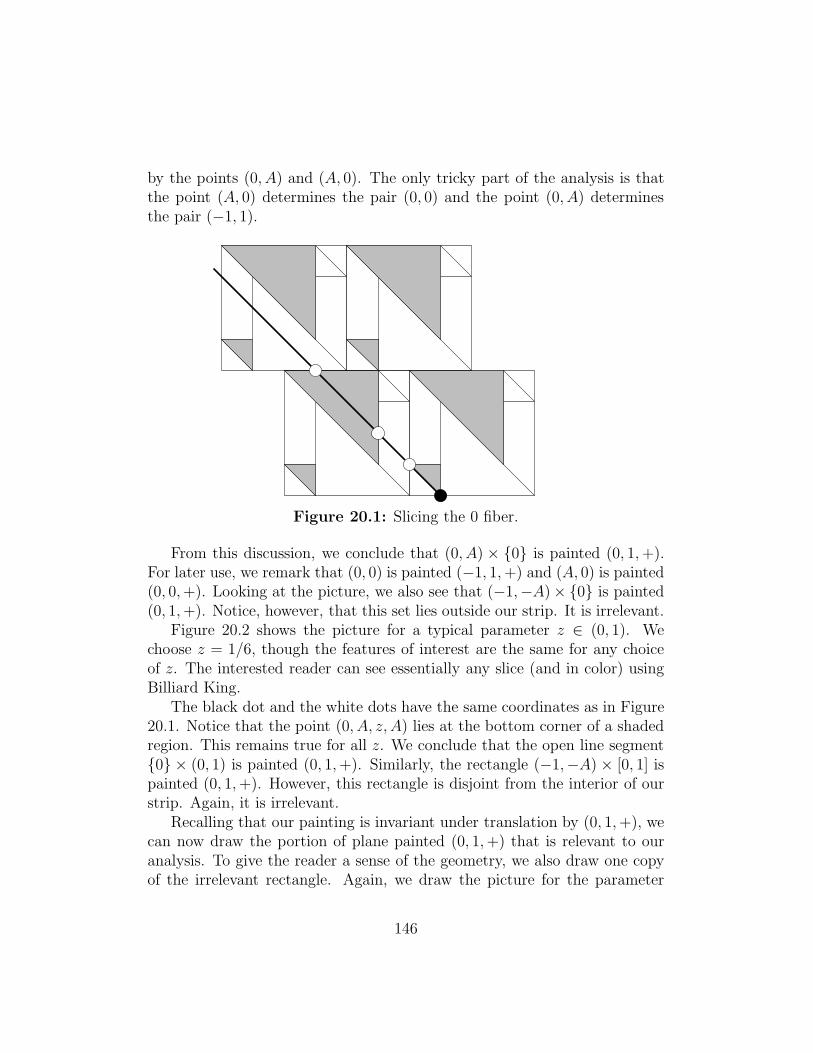
by the points (0, A) and (A, 0). The only tricky part of the analysis is thatthe point (A, 0) determines the pair (0, 0) and the point (0, A) determinesthe pair (−1, 1).

Figure 20.1: Slicing the 0 fiber.

From this discussion, we conclude that (0, A) × {0} is painted (0, 1,+).For later use, we remark that (0, 0) is painted (−1, 1,+) and (A, 0) is painted(0, 0,+). Looking at the picture, we also see that (−1,−A)× {0} is painted(0, 1,+). Notice, however, that this set lies outside our strip. It is irrelevant.

Figure 20.2 shows the picture for a typical parameter z ∈ (0, 1). Wechoose z = 1/6, though the features of interest are the same for any choiceof z. The interested reader can see essentially any slice (and in color) usingBilliard King.

The black dot and the white dots have the same coordinates as in Figure20.1. Notice that the point (0, A, z, A) lies at the bottom corner of a shadedregion. This remains true for all z. We conclude that the open line segment{0} × (0, 1) is painted (0, 1,+). Similarly, the rectangle (−1,−A) × [0, 1] ispainted (0, 1,+). However, this rectangle is disjoint from the interior of ourstrip. Again, it is irrelevant.

Recalling that our painting is invariant under translation by (0, 1,+), wecan now draw the portion of plane painted (0, 1,+) that is relevant to ouranalysis. To give the reader a sense of the geometry, we also draw one copyof the irrelevant rectangle. Again, we draw the picture for the parameter

146

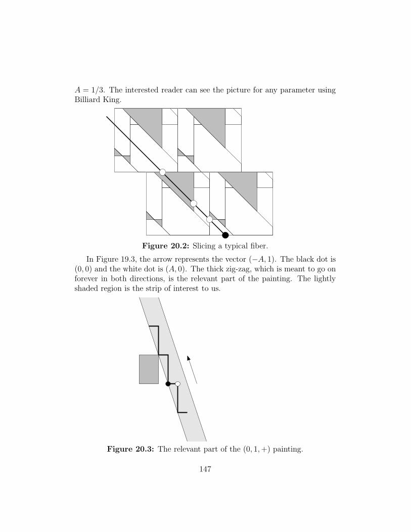
A = 1/3. The interested reader can see the picture for any parameter usingBilliard King.

Figure 20.2: Slicing a typical fiber.

In Figure 19.3, the arrow represents the vector (−A, 1). The black dot is(0, 0) and the white dot is (A, 0). The thick zig-zag, which is meant to go onforever in both directions, is the relevant part of the painting. The lightlyshaded region is the strip of interest to us.

Figure 20.3: The relevant part of the (0, 1,+) painting.

147

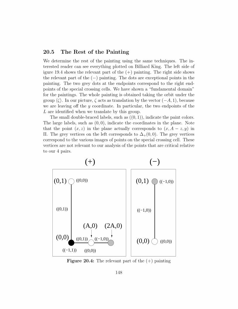
20.5 The Rest of the Painting

We determine the rest of the painting using the same techniques. The in-terested reader can see everything plotted on Billiard King. The left side ofigure 19.4 shows the relevant part of the (+) painting. The right side showsthe relevant part of the (−) painting. The dots are exceptional points in thepainting. The two grey dots at the endpoints correspond to the right end-points of the special crossing cells. We have shown a “fundamental domain”for the paintings. The whole painting is obtained taking the orbit under thegroup 〈ζ〉. In our picture, ζ acts as translation by the vector (−A, 1), becausewe are leaving off the y coordinate. In particular, the two endpoints of theL are identified when we translate by this group.

The small double-braced labels, such as ((0, 1)), indicate the paint colors.The large labels, such as (0, 0), indicate the coordinates in the plane. Notethat the point (x, z) in the plane actually corresponds to (x,A − z, y) inΠ. The grey vertices on the left corresponds to ∆+(0, 0). The grey verticescorrespond to the various images of points on the special crossing cell. Thesevertices are not relevant to our analysis of the points that are critical relativeto our 4 pairs.

(−)

((−1,0))(0,1) ((0,0))

((0,1)) ((−1,0))

(+)

((0,1))(0,0) ((−1,0)) (0,0) ((0,0))

((−1,1)) ((0,0))

(A,0) (2A,0)

(0,1)

Figure 20.4: The relevant part of the (+) painting

148

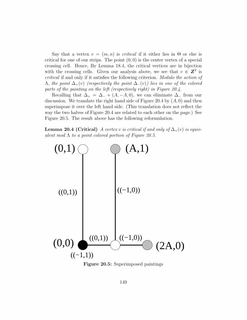
Say that a vertex v = (m,n) is critical if it either lies in Θ or else iscritical for one of our strips. The point (0, 0) is the center vertex of a specialcrossing cell. Hence, By Lemma 18.4, the critical vertices are in bijectionwith the crossing cells. Given our analysis above, we see that v ∈ Z2 iscritical if and only if it satisfies the following criterion. Modulo the action ofΛ, the point ∆+(v) (respectively the point ∆−(v)) lies in one of the coloredparts of the painting on the left (respectively right) in Figure 20.4.

Recalling that ∆+ = ∆− + (A,−A, 0), we can eliminate ∆− from ourdiscussion. We translate the right hand side of Figure 20.4 by (A, 0) and thensuperimpose it over the left hand side. (This translation does not reflect theway the two halves of Figure 20.4 are related to each other on the page.) SeeFigure 20.5. The result above has the following reformulation.

Lemma 20.4 (Critical) A vertex v is critical if and only of ∆+(v) is equiv-alent mod Λ to a point colored portion of Figure 20.5.

(A,1)

((−1,0))(2A,0)

((0,1)) ((−1,0))

(0,1)

((−1,1))

((0,1))(0,0)

Figure 20.5: Superimposed paintings

149

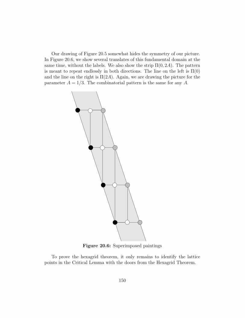
Our drawing of Figure 20.5 somewhat hides the symmetry of our picture.In Figure 20.6, we show several translates of this fundamental domain at thesame time, without the labels. We also show the strip Π(0, 2A). The patternis meant to repeat endlessly in both directions. The line on the left is Π(0)and the line on the right is Π(2A). Again, we are drawing the picture for theparameter A = 1/3. The combinatorial pattern is the same for any A.

Figure 20.6: Superimposed paintings

To prove the hexagrid theorem, it only remains to identify the latticepoints in the Critical Lemma with the doors from the Hexagrid Theorem.

150

20.6 The End of the Proof

Now we interpret the Critical Lemma algebraically. A vertex v ∈ Z2 iscritical if and only if ∆+(v) is equivalent mod Λ to one of the following kindsof points.

1. (2A,−A, 0).

2. (0, A, 0).

3. (x,A− x, 0), where x ∈ (0, 2A)− {A}.

4. (0, A, z), where z ∈ (0, 1).

As we point out in our subsection headings, each case corresponds to a dif-ferent feature of our painting in Figures 19.5 and 19.6

20.6.1 Case 1: The Grey Dots

Note that ∆+(0, 0) = (2A,−A, 0). Moreover, ∆+(v) ≡ ∆+(v′) mod Λ iffM+(v) ≡ M−(v) mod Λ iff v ≡ v′ mod Θ. Hence, Case 1 above correspondsprecisely to the special crossing cells. The door associated to v is preciselyv. In this case, the door is associated to the wall above it.

20.6.2 Case 2: The Black Dots

Note that ∆+(0,−1) = (0, A, 0). Hence the second case occurs iff v is equiv-alent mod Θ to (0,−1). But (0,−1) is the vertex of a crossing cell whoseother vertex is (−1, 0). The door associated to (0,−1) is (0, 0). In this case,the door is associated to the wall below it.

20.6.3 Case 3: Horizontal Segments

We are going to demonstrate the bijection between the Type 1 doors notcovered in Cases 1 and 2 and the critical points that arise from Case 3 above.

Let v be a critical point. Using the symmetry of Θ, we can arrange thatour point v is closer to L0 than to any other wall line. In this case, ∆+(v)lies in the strip Π(0, 2A). Hence v ∈ Σ(0, 1). Hence L0 separates v fromv + (0, 1). Let y ∈ (n, n+ 1) be such that (m, y) ∈ L0.

151

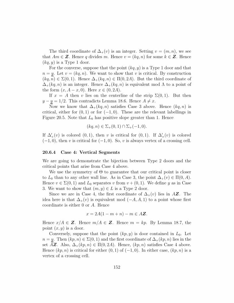
The third coordinate of ∆+(v) is an integer. Setting v = (m,n), we seethat Am ∈ Z. Hence q divides m. Hence v = (kq, n) for some k ∈ Z. Hence(kq, y) is a Type 1 door.

For the converse, suppose that the point (kq, y) is a Type 1 door and thatn = y. Let v = (kq, n). We want to show that v is critical. By construction(kq, n) ∈ Σ(0, 1). Hence ∆+(kq, n) ∈ Π(0, 2A). But the third coordinate of∆+(kq, n) is an integer. Hence ∆+(kq, n) is equivalent mod Λ to a point ofthe form (x,A− x, 0). Here x ∈ (0, 2A).

If x = A then v lies on the centerline of the strip Σ(0, 1). But theny − y = 1/2. This contradicts Lemma 18.6. Hence A 6= x.

Now we know that ∆+(kq, n) satisfies Case 3 above. Hence (kq, n) iscritical, either for (0, 1) or for (−1, 0). These are the relevant labellings inFigure 20.5. Note that L0 has positive slope greater than 1. Hence

(kq, n) ∈ Σ+(0, 1) ∩ Σ+(−1, 0).

If ∆′+(v) is colored (0, 1), then v is critical for (0, 1). If ∆′

+(v) is colored(−1, 0), then v is critical for (−1, 0). So, v is always vertex of a crossing cell.

20.6.4 Case 4: Vertical Segments

We are going to demonstrate the bijection between Type 2 doors and thecritical points that arise from Case 4 above.

We use the symmetry of Θ to guarantee that our critical point is closerto L0 than to any other wall line. As in Case 3, the point ∆+(v) ∈ Π(0, A).Hence v ∈ Σ(0, 1) and L0 separates v from v+ (0, 1). We define y as in Case3. We want to show that (m, y) ∈ L is a Type 2 door.

Since we are in Case 4, the first coordinate of ∆+(v) lies in AZ. Theidea here is that ∆+(v) is equivalent mod (−A,A, 1) to a point whose firstcoordinate is either 0 or A. Hence

x = 2A(1−m+ n)−m ∈ AZ.

Hence x/A ∈ Z. Hence m/A ∈ Z. Hence m = kp. By Lemma 18.7, thepoint (x, y) is a door.

Conversely, suppose that the point (kp, y) is door contained in L0. Letn = y. Then (kp, n) ∈ Σ(0, 1) and the first coordinate of ∆+(kp, n) lies in theset AZ. Also, ∆+(kp, n) ∈ Π(0, 2A). Hence, (kp, n) satisfies Case 4 above.Hence (kp, n) is critical for either (0, 1) of (−1, 0). In either case, (kp, n) is avertex of a crossing cell.

152

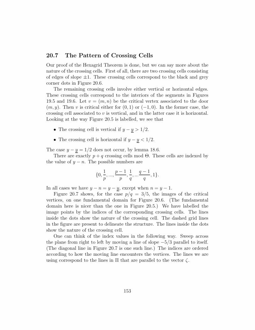
20.7 The Pattern of Crossing Cells

Our proof of the Hexagrid Theorem is done, but we can say more about thenature of the crossing cells. First of all, there are two crossing cells consistingof edges of slope ±1. These crossing cells correspond to the black and greycorner dots in Figure 20.6.

The remaining crossing cells involve either vertical or horizontal edges.These crossing cells correspond to the interiors of the segments in Figures19.5 and 19.6. Let v = (m,n) be the critical vertex associated to the door(m, y). Then v is critical either for (0, 1) or (−1, 0). In the former case, thecrossing cell associated to v is vertical, and in the latter case it is horizontal.Looking at the way Figure 20.5 is labelled, we see that

• The crossing cell is vertical if y − y > 1/2.

• The crossing cell is horizontal if y − y < 1/2.

The case y − y = 1/2 does not occur, by lemma 18.6.There are exactly p+ q crossing cells mod Θ. These cells are indexed by

the value of y − n. The possible numbers are

{0, 1p, ...,

p− 1

p,1

q, ...

q − 1

q, 1}.

In all cases we have y − n = y − y, except when n = y − 1.Figure 20.7 shows, for the case p/q = 3/5, the images of the critical

vertices, on one fundamental domain for Figure 20.6. (The fundamentaldomain here is nicer than the one in Figure 20.5.) We have labelled theimage points by the indices of the corresponding crossing cells. The linesinside the dots show the nature of the crossing cell. The dashed grid linesin the figure are present to delineate the structure. The lines inside the dotsshow the nature of the crossing cell.

One can think of the index values in the following way. Sweep acrossthe plane from right to left by moving a line of slope −5/3 parallel to itself.(The diagonal line in Figure 20.7 is one such line.) The indices are orderedaccording to how the moving line encounters the vertices. The lines we areusing correspond to the lines in Π that are parallel to the vector ζ .

153

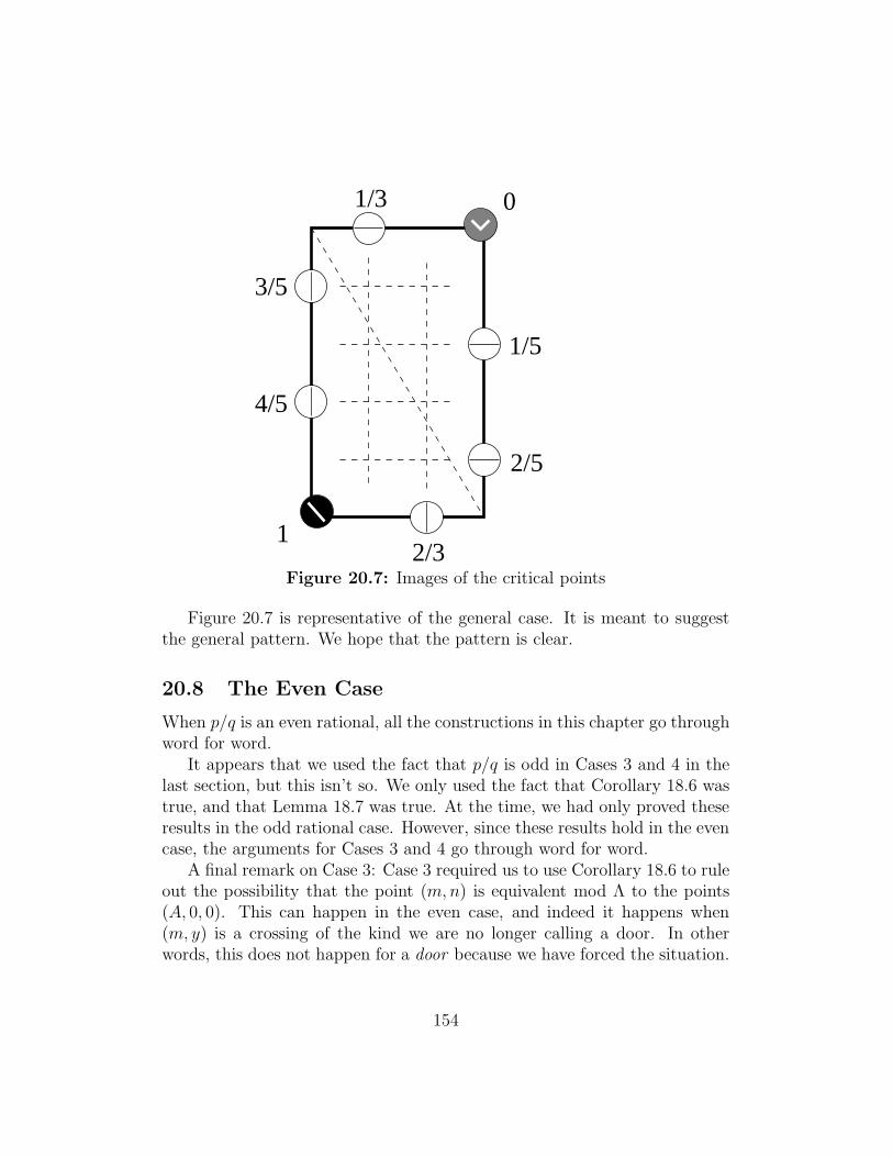
2/3

0

1

4/5

3/5

1/5

2/5

1/3

Figure 20.7: Images of the critical points

Figure 20.7 is representative of the general case. It is meant to suggestthe general pattern. We hope that the pattern is clear.

20.8 The Even Case

When p/q is an even rational, all the constructions in this chapter go throughword for word.

It appears that we used the fact that p/q is odd in Cases 3 and 4 in thelast section, but this isn’t so. We only used the fact that Corollary 18.6 wastrue, and that Lemma 18.7 was true. At the time, we had only proved theseresults in the odd rational case. However, since these results hold in the evencase, the arguments for Cases 3 and 4 go through word for word.

A final remark on Case 3: Case 3 required us to use Corollary 18.6 to ruleout the possibility that the point (m,n) is equivalent mod Λ to the points(A, 0, 0). This can happen in the even case, and indeed it happens when(m, y) is a crossing of the kind we are no longer calling a door. In otherwords, this does not happen for a door because we have forced the situation.

154

Part IVIn this part of the monograph we use the Master Picture Theorem to provethe Copy Theorems and the Decomposition Theorem, two technical resultsleft over Part I. The Copy Theorems were discussed in §7. The Decomposi-tion Theorem was discussed in §8.3.

• In §21 we state and prove the Copy Theorem, our main period copyingtheorem. We will also deduce Theorem 4.3 from the Copy Theorem.As we mentioned in Part I, Theorem 4.3 is sufficient to prove our mainresults for almost every parameter. The reader who is satisfied knowingour main results for almost every A ∈ (0, 1) can stop reading afterthis chapter. One can view the rest of Part of IV as a more carefulaccounting of what is going on, in order to improve the main resultsfrom “almost every” to ”every”.

• In §22 we will prove the Superior Sequence Lemma. We will also es-tablish a few auxilliary results about the superior sequences.

• In §23 we will prove the Decomposition Theorem from §8. The CopyTheorem does imply Theorems 4.2 and 7.5, but (as far as we can see)not in any direct way. We need to combine the Copy Theorem withthe Decomposition Theorem.

• In 24.1, we will deduce Theorem 4.2 from the Copy Theorem, the De-composition Theorem, and from the theory built up in §22. At the endof this chapter, we will have tied up all the loose ends in the monograph.

155

21 The Copy Theorem

21.1 Two Linear Functionals

Let p/q be an odd rational. Let V = (q,−p) be the vector from Equation12. In terms of the arithmetic kite, V = v7. Our period copying theoremswill be stated in terms of the following 2 linear functionals.

G(m,n) =(q − pp+ q

,−2q

p+ q

)· (m,n). (187)

H =(−p2 + 4pq+q2

(p+ q)2,2q(q − p)(p+ q)2

)· (m,n). (188)

These two functions are adapted to the arithmetic kite.

Lemma 21.1 G(V ) = q. Moreover, the fibers of G are parallel to the topleft edge of the arithmetic kite.

Proof: The first statement is a computation. Referring to the arithmetickite in Figure 4.1, we compute that G(v6) = G(v3). Thus, G takes on thesame values on the top left edge of Q(p/q). ♠

Lemma 21.2 H(V ) = q. Moreover, the fibers of H are parallel to the topright edge of the arithmetic kite.

Proof: The first statement is a computation. Referring to the arithmetickite in Figure 4.1, we compute that H(v7) = H(v3). Thus, H takes on thesame values on the top left right of Q(p/q). ♠

Given r < 0 < s, we define

∆(r, s) = {(m,n)| G(m,n), H(m,n) ∈ [r, s]}. (189)

This set is a parallelogram that is cut in half by the baseline of Γ(p/q). Foraplications, we are mainly interested in points of ∆(r, s) above the baseline,but our result works for points below the baseline as well.

156

21.2 The Main Result

Suppose that A1 = p1/q1 is an odd rational and A2 = p2/q2 is anotherrational, not necessarily odd. We define a = a(A1, A2) by the formula

∣∣∣∣p1

q1− p2

q2

∣∣∣∣ =2

aq21

. (190)

We call (A1, A2) a good pair if a > 1 and q2 ≥ aq1. In case A2 is odd, thesecond condition is automatic. Referring to the notation in Equation 18, wedefine

λ1 =(q1)+

q1. (191)

If A1 < A2 we define

K = floor(a

2− λ1

)+ 1 + λ1. (192)

if A1 > A2 we define

K = floor(a

2+ λ1

)+ 1− λ1. (193)

Theorem 21.3 (Copy) Let C = 3. Let (A1, A2) be a good pair of rationals.Then

1. If A1 < A2 then Γ1 and Γ2 agree on ∆(−q1 + C,Kq1 − C).

2. If A1 > A2 then Γ1 and Γ2 agree on ∆(−Kq1 + C, q1 − C).

Remarks: (i) Our result has the following geometric interpretation. Tomake the interpretation work best, set C = 0, and let ∆ be the set fromthe Copy Theorem. Let Lj be the baseline for Γj. Then both L1 and L2

essentially bisect ∆, and no lattice point lies between L1 ∩ ∆ and L2 ∩ ∆.Enlarging ∆ at all would destroy this property. So, for fixed shape, ∆ is themaximal parallelogram with the lattice point property we just mentioned.(ii) The constant C = 3 is an artifact of our proof. Probably C = 2 is theoptimal constant. For our applications, we just need the existence of someconstant C.

157

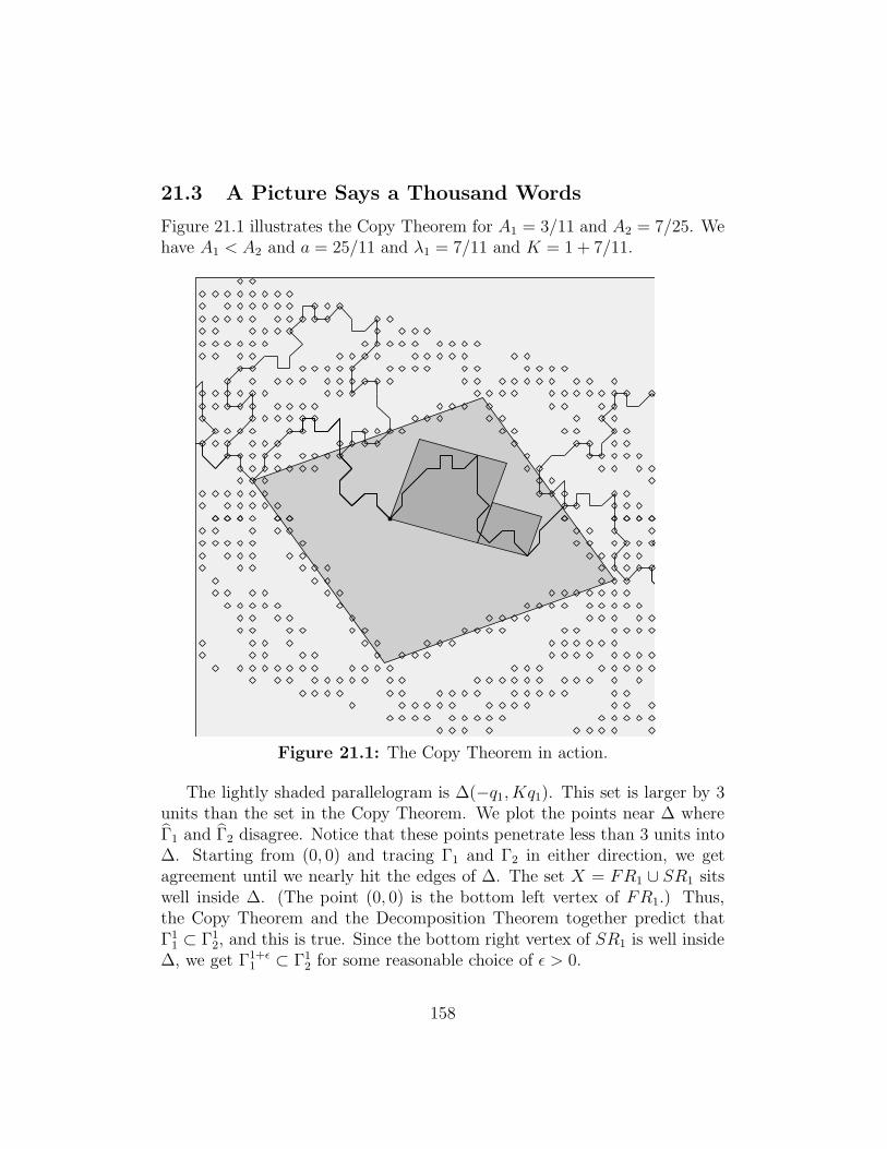
21.3 A Picture Says a Thousand Words

Figure 21.1 illustrates the Copy Theorem for A1 = 3/11 and A2 = 7/25. Wehave A1 < A2 and a = 25/11 and λ1 = 7/11 and K = 1 + 7/11.

Figure 21.1: The Copy Theorem in action.

The lightly shaded parallelogram is ∆(−q1, Kq1). This set is larger by 3units than the set in the Copy Theorem. We plot the points near ∆ whereΓ1 and Γ2 disagree. Notice that these points penetrate less than 3 units into∆. Starting from (0, 0) and tracing Γ1 and Γ2 in either direction, we getagreement until we nearly hit the edges of ∆. The set X = FR1 ∪ SR1 sitswell inside ∆. (The point (0, 0) is the bottom left vertex of FR1.) Thus,the Copy Theorem and the Decomposition Theorem together predict thatΓ1

1 ⊂ Γ12, and this is true. Since the bottom right vertex of SR1 is well inside

∆, we get Γ1+ǫ1 ⊂ Γ1

2 for some reasonable choice of ǫ > 0.

158

21.4 Proof of Theorem 4.3

Let V1 and W1 be the vectors in Equation 12. By the Room Lemma andperiodicity, Γn

1 ⊂ Rn, where Rn is the parallelogram bounded by the vectors

(0, 0); nV1; W1; nV1 +W1. (194)

Since a = 2n + 2, we have K ≥ n + 1 in the Copy Theorem. For ease ofnotation, we set p = p1 and G = G1, etc. Let

I = [−q + 3, Kq − 3].

Obviously G(0, 0) = H(0, 0) = 0 ∈ I. For the remaining vertices, we have

G(nV ) = H(nv) = nq ∈ I

G(W ) = − q2

p + q∈∗ [−q + 3, 0] ⊂ I

H(W ) = +q2

p+ q∈∗ [0, q − 3] ⊂ I.

G(W + nV ) = G(W ) +G(nV ) ∈∗ [nq − q + 3, nq] ⊂ I.

H(W + nV ) = H(W ) +H(nV ) ∈∗ [nq, nq + q − 3] ⊂ I.

The starred containments hold for p large.We also have universal gradient bounds

‖∇G‖ < 8 ‖∇H‖ < 8. (195)

Combining these bounds with our calculations for the bottom right vertexnV , we see that any vertex within ǫq units of nV lies in ∆(−q + 3, Kq − 3).Here ǫ = 1/10. In short,

(m,n) ∈ ∆(−q1 + 3, Kq1 − 3); ∀ (m,n) ∈ Γn+ǫ1 . (196)

By the Copy Theorem, Γn+ǫ1 ⊂ Γ2. Since Γ1 and Γ2 both contain the (0, 0),

we now see that Γn+ǫ1 ⊂ Γ2. But the right endpoint of Γ1+ǫ

1 is within ǫq1 ofnV1 whereas the right endpoint of Γ1

2 is (much) more than ǫq1 from nV1, andfurther to the right. Hence Γn+ǫ

1 ⊂ Γ12.

159

21.5 Setting up the Main Proof

For ease of exposition, we only prove Statement 1 of the Copy Theorem,which we refer to as the Copy Theorem I. The Copy Theorem II has analmost identical proof. We will use the method in §10.5 to compute thearithmetic graphs Γ1 and Γ2. By the Master Picture Theorem, it suffices toshow that the points M±(m,n) land in the same polyhedron of RA, relativeto A1 = p1/q1 and A2 = p2/q2. The following 10 step outline explains howwe do this. Here ǫ1 and ǫ2 stand for integers in {−1, 0, 1}.

1. Let zj = Ajm+ n.

2. Let Zj = floor(xj).

3. We prove that Z1 = Z2. Let Z = Z1 = Z2. We also prove that thestatement zj − Z < ǫ1Aj + ǫ2 has the same truth value independent ofj ∈ {1, 2}. We mean this to hold for any relevant choice of ǫ1 and ǫ2.

4. Let yj = zj + Zj in the (−) case and yj = zj + Zj + 1 in the (+) case.

5. Let Yj = floor(yj/(1 + Aj).

6. We prove that Y1 = Y2. Let Y = Y1 = Y2. We also prove thatthe statement yj − Y (1 + Aj) < ǫ1Aj + ǫ2 has the same truth valueindependent of j ∈ {1, 2}. We mean this to hold for any relevantchoice of ǫ1 and ǫ2.

7. Let xj = yj − Y (1−Aj)− 1.

8. Let Xj = floor(xj/(1 + Aj)).

9. We prove that X1 = X2. Let X = X1 = X2. We also prove that

xj −X(1 + Aj) < ǫ1Aj + ǫ2

has the same truth value independent of j ∈ {1, 2}. We mean this tohold for any relevant choice of ǫ1 and ǫ2.

10. We want to see that all of the statements

(xj −X(1 + Aj)) + (yj − Y (1 + Aj))− (zj − Z) < h+ Aj; h ∈ Z

has the same truth value independent of j ∈ {1, 2}.

160

21.6 Good Integers

In this section we state 3 technical lemmas that imply the Copy Theorem I.Our notation refers to the 10 step outline above.

Let Aj = pj/qj for j = 1, 2. We say that an integer µ is good if

floor(µA1) = floor(µA2). (197)

Lemma 21.4 (Good Integer) Suppose (m,n) satisfies the hypotheses ofthe Copy Theorem I, and X1 and Y1 are the integers that arise when weperform the reduction algorithm above to (m,n). For any ǫ ∈ {−1, 0, 1}, theintegers

m− ǫ; m− Y1 − ǫ; m−X1 − ǫ; m+ Y1 −X1 + ǫ

are all good integers.

Proof: See §21.8. ♠

Lemma 21.5 Let d ≥ 0 be an integer. Suppose µ, η ∈ Z. Let Nj be theinteger such that

Nj(dAj + 1) < µAj + ν + α < (Nj + 1)(dAj + 1).

Suppose µ− dN1 and µ− dN2 are both good integers. Then N1 = N2.

Proof: Suppose first that N1 < N2. In this case we set N = N2 and we notethat

µA1 + ν < N(dA1 + 1); N(dA2 + 1) > µA2 + ν.

But then(µ− dN)A1 < N − ν < (µ− dN)A2.

This contradicts the fact that µ − dN2 is good. If N1 > N2 we set N = N1

and get the same equations with the inequalities reversed. This contradictsthe fact that µ− dN1 is good. ♠

161

Lemma 21.6 Let d ≥ 0 be an integer and. Suppose µ, η ∈ Z. Let N be aninteger. The truth of the statement

(µAj + η + α)−N(dAj + 1) < ǫ1A1 + ǫ2

is independent of j provided that µ− dN − ǫ1 is good.

Proof: The proof is almost the same as in Lemma 21.5. If the above state-ment is true for j = 1 and false for j = 2 then we get the inequalities

(µ− dN − ǫ1)A1 < ǫ2 +N − ν < (µ− dN − ǫ1)A2,

and this contradicts the fact that µ− dN − ǫ1 is good. We get a similar con-tradiction, with the inequalities reversed, if the statement is true for j = 1and false for j = 2. ♠

21.7 The Main Argument

We will carry out the 10 step outline for M−. The argument for M+ isessentially identical.

• We have zj = mAj +n. To see that Z1 = Z2 we apply the Good IntegerLemma and Lemma 21.5 to the case

(µ, d,Nj) = (m, 0, Zj).

The relevant good integer is m. Let Z = Z1 = Z2.

• To see that the truth of the statement zj − Z < ǫ1Aj + ǫ2 is trueindependent of j, we apply the Good Integer Lemma and Lemma 21.6to the case

(µ, d,N) = (m, 0, Z).

The relevant good integer is m− ǫ1.

• We have yj = mAj +n′ for some n′ ∈ Z. To see that Y1 = Y2 we applythe Good Integer Lemma and Lemma 21.5 to the case

(µ, d,Nj) = (m, 1, Yj).

The relevant good integers are m−Y1 and m−Y2. We set Y = Y1 = Y2.

162

• To see that the truth of the statement yj − Y (A1 + 1) < ǫ1Aj + ǫ2 isindependent of j, we apply the Good Integer Lemma and Lemma 21.6to the case

(µ, d,N) = (m, 1, Y ).

The relevant good integer is m− Y − ǫ1.

• We havexj = (m+ Y )Aj + n′′

for some n′′ ∈ Z. To see that X1 = X2 we apply the Good IntegerLemma and Lemma 21.5 to the case

(µ, d,Nj) = (m+ Y, 1, Xj).

The relevant good numbers are m+ Y −X1 and m+ Y −X2. We setX = X1 = X2.

• To see that the truth of the statement xj − (1 + Aj)X < ǫ1Aj + ǫ2 isindependent of j = 1, 2 we apply the Good Integer Lemma and Lemma21.6 to the case

(µ, d,N) = (m+ Y, 1, X).

The relevant good number is m+ Y −X − ǫ1.

• Define

σj = (xj −X(1 + Aj)) + (yj − Y (1 + Aj))− (zj − Z).

We have σj = (m−X)Aj+n′′′ for some n′′′ ∈ Z. Let h ∈ Z be arbitrary.

To see that the truth of the statement σj < Aj + h is independent of jwe apply the Good Integer Lemma and Lemma 21.6 to

(µ, d,N) = (m−X, 1, 0).

The relevant good number is m−X − 1.

This proves that M−(m,n) lands in the same polyhedron for each parameterA1 and A2. As we said above, essentially the same argument works forM+. Modulo the Good Integer Lemma, this completes the proof of the CopyTheorem I. Again, the proof of the the Copy Theorem II is almost identical.

It only remains to prove the Good Integer Lemma.

163

21.8 Proof of the Good Integer Lemma

21.8.1 Step 1

Let K be as in the Copy Theorem I.

Lemma 21.7 If µ ∈ (−q1, Kq1) ∩Z then µ is a good integer.

We will prove this result in two stages, one for the lower bound for onefor the upper bound.

Lemma 21.8 If µ ∈ (−q1, 0), then µ is good.

Proof: Since q1 is odd, we have unique integers j and M such that

µA1 = M +j

q1; |j| < q1

2. (198)

By hypotheses, a > 1. Hence

|A2 − A1| < 2/q21 (199)

in all cases. If this result is false, then there is some integer N such that

µA2 < N ≤ µA1. (200)

Referring to Equation 198, we have

|j|q1

< µA1 −N ≤ µA1 − µA2 <2|µ|q21

<2

q1. (201)

If j = 0 then q1 divides µ, which is impossible. Hence |j| = 1. If j = −1then µA1 is 1/q1 less than an integer. Hence µA1−N ≥ (q1 − 1)/q1. This isfalse, so we must have j = 1.

From the definition of λ1, we have the following implication.

µ ∈ (−q1, 0) and µp1 ≡ 1 mod q1 =⇒ µ = −λ1q1. (202)

Equation 198 impliesµp1

q1− 1

q1∈ Z.

But then µp1 ≡ 1 mod q1. Equation 202 now tells us that µ = −λ1q1. Hence|µ| < q1/2. But now Equation 201 is twice as strong and gives |j| = 0. Thisis a contradiction. ♠

164

Lemma 21.9 If µ ∈ (0, Kq1) then µ is good.

Proof: We observe that K < a, by Equation 192. If this result is false, thenthere is some integer N such that µA1 < N ≤ µA2. If µA2 = N . Then q2divides µ. But then,

µ ≥ q2 ≥ aq1 > Kq1.

This is a contradiction. Hence

µA1 < N < µA2. (203)

Referring to Equation 198, we have

|j|q1≤ N − µA1 < µ(A2 − A1) =

2µ

aq21

<2

q1. (204)

Suppose that j ∈ {0, 1} in Equation 198. Then

1− 1

q1≤ N − µA1 ≤ µA2 − µA1 <

1

q1,

a contradiction. Hence j = −1. Hence µ > aq1/2.Since j = −1, Equation 198 now tells us that µp1 + 1 ≡ 0 mod q1. But

thenµ = kq1 + (q1)+, (205)

for some k ∈ Z. On the other hand, from Equation 192 and the fact thatµ < Kq1, we have

µ < k′q1 + (q1)+; k′ =(floor(a/2− λ1) + 1

). (206)

Comparing the last two equations, we have k ≤ k′ − 1. Hence

k ≤(floor(a/2− λ1)

). (207)

Thereforeµ ≤

(floor(a/2− λ1)

)q1 + λ1q1 ≤ aq1/2.

But we have already shown that µ > aq1/2. This is a contradiction. ♠

165

21.8.2 Step 2

The Good Integer Lemma only involves the numbers p1, q1, X1, etc. For easeof notation, we set p = p1, etc.

The Good Integer Lemmma involves 4 statements, one per listed number.Statement 1 follows immediately from Lemma 21.7. By construction, we haveX ∈ [−1, Y ]. Hence m − X ∈ [m − Y,m + 1]. Hence, Statement 2 impliesStatement 3. Our next two results deal respectively with Statements 2 and4. In these results, ǫ can be any of the three integers in {−1, 0, 1}. Thereduction algorithm from §21.5 must be performed for the map M− and forthe map M+.

Lemma 21.10 G(m,n) ∈ (−q1 + 2, Kq1 − 3) then m− Y1 − ǫ is good.

Proof: We will treat the (+) case. In the (−) case, the only difference isthat Y + 1 replaces Y . We will use the terminology Reduce k to refer tothe kth step in our outline from §21.5. Given that we are working with M−,Reduce 4 gives us

y ∈ [2z − 1, 2z] (208)

Reduce 5 gives us

Y ∈[

y

1 + A− 1,

y

1 + A

]⊂

[2z

1 + A− 1− 1

1 + A,

2z

1 + A

]. (209)

Using z = Am+ n and A = p/q, we get

m− Y ∈[G−(m,n), G−(m,n) + 1 +

1

1 + A

]. (210)

If G−(m,n) > −q + 1 then

m− Y − ǫ > −q + 1.

If G−(m,n) < Kq − 3 then

m− Y − ǫ < Kq − 2 + 1 +1

1 + A< Kq.

Since m− Y − ǫ is an integer, we have m− Y − ǫ < Kq. All in all, we havem− Y − ǫ ∈ (−q,Kq). Lemma 21.7 now applies. ♠

166

Lemma 21.11 If H(m,n) ∈ (−q1 + 3, Kq1 − 3) then m + Y1 − X1 − ǫ isgood.

Proof: Our proof works the same in the (+) and (−) cases. Reduce 5 andReduce 8 give us

Y ∈[

y

1 + A− 1,

y

1 + A

]; X ∈

[x

1 + A− 1,

x

1 + A

].

Hence

Y −X ∈[y − x1 + A

− 1,y − x1 + A

+ 1]

(211)

Reduce 7 gives usy − x1 + A

= Y1− A1 + A

+1

1 + A(212)

Equation 209 gives us

Y1− A1 + A

∈[2z

1−A(1 + A)2

− η, 2z 1−A(1 + A)2

]; η =

(1 +

1

1 + A

)× 1−A

1 + A.

Observing that

1

1 + A− η =

A2 + 2A− 1

(1 + A)2∈ (−1,

1

2),

we see that

m+y − x1 + A

∈(2z

1− A(1 + A)2

− 1, 2z1−A

(1 + A)2+

1

2

)=

(G+ (m,n)− 1, G+ (m,n) +

1

2

). (213)

Combining this last result with Equation 211, we have

m+ Y −X ∈(G + (m,n)− 2, G+ (m,n) +

3

2

). (214)

The rest of the proof is as in Lemma 21.10. ♠

167

22 Existence of Superior Sequences

22.1 Outline

In this chapter we will prove the Superior Sequence Lemma, and also derivesome basic properties of superior sequences. Our construction of the superiorsequence is a 2-step process. First we will construct a sequence {pn/qn} suchthat pn/qn ← pn+1/qn+1 for all n, in the sense of Equation 20. Explicitly, wehave

λn < 1/2 =⇒ pn−1

qn−1=

(pn)+ − (pn)−(qn)+ − (qn)−

(215)

λn > 1/2 =⇒ pn−1

qn−1

=(pn)− − (pn)+

(qn)− − (qn)+

(216)

Here

λn =(qn)+

qn. (217)

We call this sequence the inferior sequence. We will produce a superiorsequence by taking a suitable subsequence of the inferior sequence. Thereader should look again at the example we gave right after the statementof the Superior Sequence Lemma. We took this 2-step approach in thatexample.

Even though we are ultimately only interested in the superior sequence,we will state many of our structural results in terms of the inferior sequence.The idea is that we can use properties of the inferior sequence to deduceproperties of the superior sequence.

We will use elementary hyperbolic geometry to show the existence ofthe inferior sequence. This is similar to what one does for the sequenceof continued fraction approximants. Here is a rapid review of hyperbolicgeometry. The reader should consult [B] for details.

The hyperbolic plane is the upper halfplane H2 ⊂ C. The group SL2(R)of real 2 × 2 matrices acts isometrically by linear transformations. Thegeodesics are vertical rays or semicircles centered on R.

The Farey graph is a tiling of H2 by ideal triangles. We join p1/q1 andp2/q2 by a geodesic iff |p1q2 − p2q1| = 1. The resulting graph divides thehyperbolic plane into an infinite symmetric union of ideal geodesic triangles.The Farey graph is probably the most famous picture in hyperbolic geometry.

168

22.2 Existence of the Inferior Sequence

We modify the Farey graph by erasing all the lines that connect even frac-tions to each other. The remaining edges partition H2 into an infinite unionof ideal squares.

Remark: The pattern of idea squares is not preserved by the modulargroup. However, the level 2 congruence subgroup Γ2 does preserve the pat-tern of squares. Indeed, a single square serves as a fundamental domain forthe action of Γ2, and the quotient H2/Γ2 is a 3-punctured sphere obtainedby suitably identifying the boundaries of the square.

We say that a basic square is one of these squares that has all verticesin the interval (0, 1). Each basic square has two opposing vertices that arelabelled by positive odd rationals, p1/q1 and p2/q2. These odd rationalssatisfy Equation 18 when ordered so that q1 < q2. We call p1/q1 the headof the square and p2/q2 the tail of the square. We draw an arrow in eachodd square that points from the tail to the head. We call the odd squareright biased if the rightmost vertex is an odd rational, and left biased if theleftmost vertex is an odd rational.

The general form of a left biased square is

a1

b1;

a1 + a2

b1 + b2;

a1 + 2a2

b1 + 2b2;

a2

b2. (218)

The leftmost vertex in a left-biased square is the head, and the rightmostvertex in a right-biased square is the head. One gets the equation for aright-biased square just by reversing Equation 218.

For an irrational parameter A, we simply drop the vertical line down from∞ to A, and record the sequence of basic squares we encounter. To form theapproximating sequence, we list the heads of the encountered squares andweed out repeaters.

Referring to Equation 22, we define

κn = floor(a(An, An+1)) =∗ floor(qn+1/qn). (219)

The starred equality comes from Equation 190 and the fact that

|pnqn+1 − qnpn+1| = 2.

169

22.3 An Algorithm

Even though the material in this section does not contribute to our overallproof, it seems worthwhile to explain in practice how one computes the in-ferior sequence for a given rational parameter p/q. To produce the initialportion of the inferior sequence for an irrational parameter, we would take avery nearby rational and then follow the method we are about to describe.Here is the algorithm.

1. Given p/q, solve the congruence xp + 1 ≡ 0 mod q for x ∈ (0, q).

2. Set q+ = x and q− = q − x.

3. Find the integer y ∈ (0, p) such that xp+ 1 = yq.

4. Set p+ = y and p− = p− y.

5. Set p′ = |p+ − p−| and q′ = |q+ − q−].

6. We now have p/q → p′/q′.

7. Iterate, so as to construct p/q → p′/q′ → p′′/q′′... until 1/1 is reached.

Let’s watch this algorithm in action for p/q = 17/37. We have

13× 17− 1 = 6× 37.

Hence x = 13 and y = 6. This gives

q+ = 17; q− = 24; p+ = 6; p− = 11.

Thereforep′

q′=|6− 11||13− 24| =

5

11.

Iterating, we have17

37→ 5

11→ 3

7→ 1

3→ 1

1.

Billiard King is set up to do these computations interactively. We refer theinterested reader to Billiard King for more examples.

170

22.4 Structure of the Inferior Sequence

Now suppose that {An = pn/qn} is the inferior sequence approximating A.We index so that p0/q0 = 1/1. When n > 0, let (An)± = (pn)±/(qn)±.

Lemma 22.1 Either An < A < (An)+ or (An)− < A < An.

Proof: We will consider the case when An < An−1. The other case is similar.Let γ be the vertical geodesic to A. At some point γ encounters the basicsquare with vertices

(An)− < An < (An)+ < An−1.

If An+1 < An, then γ exits S between (An)− and An. Hence (An)− < A < An.If An+1 > An, then γ exits S to the right of An. If γ exits S to the right of(An)+, then γ next encounters a basic square S ′ with vertices

(An)+ < O < E < An−1,

where O and E are odd and even rationals. But then An would not be theterm in our sequence after An−1. The term after An−1 would lie in the interval[O,An−1). This is a contradiction. Hence γ exits S between An and (An)+. ♠

Lemma 22.2 The following is true for any m ≥ 1.

1. If An−1 < Am < Am+1 then (qm)+ < (qm)− and κm ≡ 1 mod 2 and

2(qm+1)+ = (κm + 1)(qm)+ + (κm − 1)(qm)−.

2. If An−1 > Am < Am+1 then (qm)+ > (qm)− and κm ≡ 0 mod 2 and

2(qm+1)+ = (κm + 0)(qm)− + (κm − 2)(qm)+.

3. If An−1 > Am > Am+1 then (qm)+ > (qm)− then κm ≡ 1 mod 2 and

2(qm+1)− = (κm + 1)(qm)− + (κm − 1)(qm)+.

4. If An−1 < Am > Am+1 then (qm)+ < (qm)− then κm ≡ 0 mod 2 and

2(qm+1)− = (κm + 0)(qm)+ + (κm − 2)(qm)−.

171

Proof: The first implication, in all cases, is contained in Equation 216. Forthe other implications, Cases 3 and 4 follow from Cases 1 and 2 by symmetry.For ease of exposition, we will just treat Case 1.

The vertical geodesic γ to A passes through the basic square S withvertices

pn−1

qn−1<

(pm)−(qm)−

<pm

qm<

(pm)+

(qm)+.

Since Am+1 > Am, the geodesic γ next crosses through the geodesic αm

connecting pm/qm to (pm)+/(qm)+. Following this, γ encounters the basicsquares S ′

k for k = 0, 1, 2... until it crosses a geodesic that does not havepm/qm as a left endpoint. By Equation 218 and induction, we get

S ′

k :pm

qm<

(k + 1)pm + (pm)+

(k + 1)qm + (qm)+<

(2k + 1)pm + 2(pm)+

(2k + 1)qm + 2(qm)+<kpm + (pm)+

kqm + (qm)+.

(220)Here S ′

k is a left-biased square. But then there is some k such that

pm+1

qm+1

=(2k + 1)pm + 2(pm)+

(2k + 1)qm + 2(qm)+

;(pm+1)+

(qm+1)+

=kpm + (pm)+

kqm + (qm)+

(221)

Since (qm)+ < (qm)−, we have 2(qm)+ < qm. Since 2(qm)+ < qm, we have

pm+1

qm+1− pm

qm=

2

(2k + 1)q2m + 2qm(qm)+

∈(

2

(2k + 2)q2m

,2

(2k + 1)qm

). (222)

Hence κm = (2k + 1) ≡ 1 mod 2. Finally,

2(qm+1)+ = 2kqm + 2(qm)+ = (κm + 1)(qm)+ + (κm − 1)(qm)−.

This completes the proof. ♠

22.5 The Superior Sequences

Below we will prove that κn ≥ 2 infinitely often. Hence, we can find aninfinite subsequence of the inferior sequence that has the general property

pkn

qkn

⇐=pkm+1

qkm+1

∀ n.

Passing to any further subsequence retains this property. So, we can pass toa further subsequence to produce a monotone example.

172

Lemma 22.3 κn ≥ 2 infinitely often.

Proof: We can sort the indices of our sequence into 4 types, dependingon which case holds in Lemma 22.2. We distinguish between two kinds ofapproximating sequences. If this lemma is false, then n eventually has oddtype. But, it is impossible for n to have Type 1 and for n + 1 to have Type3. Hence, eventually n has constant type, say Type 1. (The Type 3 case hasa similar treatment.) Looking at the formula in Case 1 of Lemma 22.2, wesee that the sequence {(qn)+} is eventually constant. But then

r = limn→∞

(qn)+pn

qn

exists. Since (qn)+pn ≡ −1 mod qn and qn → ∞, we must have r ∈ Z. Butthen lim pn/qn ∈ Q, and we have a contradiction. ♠

It only remains to prove the Diophantine estimate in the Superior Lemma.Here it is.

Lemma 22.4 If κm ≥ 2 and m < n, then∣∣∣∣pn

qn− pm

qm

∣∣∣∣ <2

q2m

;

∣∣∣∣A−pm

qm

∣∣∣∣ <2

q2m

Proof: By passing to the limit, we see that the second conclusion (whichdoes not involve n) is implied by the first conclusion. Therefore, it suffices toestablish the first conclusion. Suppose thatm has Type 2. Then 2(qm)+ > qmand Am < An < (Am)+. Hence

|Am −An| < |Am − (Am)+| =1

qm(qm)+

<2

q2m

.

The proof when n has Type 4 is similar.Suppose that m has Type 1. Then κm ≥ 3. Combining Lemma 22.1 and

Equation 220, we have

|Am − An| <∣∣∣∣kpm + (pm)+

kqm + (qm)+

− pm

qm

∣∣∣∣ =1

qm(kqm + (qm)+)<

1

kq2m

.

Recall that κm = 2k + 1. Hence k ≥ 1. The proof when n has Type 3 issimilar. This completes the proof. ♠

173

22.6 An Example

In terms of the notation in §4.2, we have pm/pm ⇐= pn/qn if and only ifκm = 2 and m < n. Theorems 4.2 and 7.5 concern precisely such pairs ofrationals. In this section we will study a slightly more restricted notion. Wewrite pm/qm ⇐=!pn/qn if and only if m < n and κm ≥ 2 and κj = 1 whenj = m+ 1, ..., n− 1. Put another way, we have pm/qm ⇐=!pn/qn if and onlyif n is the smallest index greater than m such that pm/qm ⇐= pn/qn. Toavoid trivialities, we only use this notation when m ≥ 1.

By Lemma 22.4, the pair (Am, An) is good provided that Am ⇐= An. Incase Am ⇐=!An, we have a nice formula for K = K(Am, An). We work outan example to motivate the general formula. Consider the sequence

A12 =1111

2347→ 951

2009→ 791

1671→ 631

1333→ 471

995→ 311

657→ 151

319= A6.

Note that A6 ⇐=!A12,For the purposes of applying Theorem 4.2, we write

A = p/q = A12; A′ = p′/q′ = A6.

To relate this directly to the notation of Theorem 4.2, we would be consid-ering the rationals p1/q1 = p′/q′ and p2/q2 = p/q. We find the alternatenotation here more convenient, because we want to distinguish p1/q1, thesubject of Theorem 4.2, from the first term in the inferior sequence. Accord-ing to this notation, all the quantities associated with the first rational are“primed”. For instance λ′ = λ(p′/q′) = q′+/q

′.We compute q′+ = 169. Hence

λ′ =169

319;

a

2=

1

q′2(A−A′)=

2347

3828;

= floor(

2347

3828− 169

319

)+ 1 +

169

319=

488

319.

We also compute that q+ = 169. Since A′ < A, we use Equation 192 tocompute K. We get

K = 1 +169

319= 1 +

q+q′.

This is a formula we want to establish in general.

174

22.7 A Useful Equality

Lemma 22.5 (Equality) Suppose that A′ ⇐=!A.

1. If A′ < A then K = 1 + q+/q′.

2. If A′ > A then K = 1 + q−/q′.

We will prove the first statement. The second statement has an extremelysimilar proof. We have part of an inferior sequence

A = An → ...→ Am = A′. (223)

Lemma 22.6 Suppose n = m+ 1 and κm is odd. Then Lemma 22.5 holds.

Proof: A′ and A are consecutive terms of the inferior sequence, Case 1 ofLemma 22.2 applies to pm/qm = p′/q′ and pm+1/qm+1 = p/q. Using the factthat 2q′ = 2q′+ + 2q′−, we have

2q+ + 2q′ = (κm + 1)q′ + 2q′+.

Dividing both sides by 2q′ gives

1 +q+q′

=κm + 1

2+q′+q′

=κm + 1

2+ λ′. (224)

Note that a = a(A′, A) lies in [κm, κm + 1). Hence, the fractional part of a/2lies in [1/2, 1). Since λ′ < 1/2, by Case 1 of Lemma 22.2,

floor(a/2− λ′) =κm − 1

2. (225)

Therefore

K = floor(a/2− λ′) + 1 + λ′ =κm + 1

2+ λ′ = 1 +

q+q′.

This completes the proof. ♠

When Am < Am+1, we define am and am by the following equation.

Am+1 − Am =2

amq+m

; (Am+1)+ − Am =2

amq+m

. (226)

175

Lemma 22.7 Suppose that Am < Am+1. Then

floor(am/2− λm) = floor(am/2− λm).

Proof: Am and (Am+1)+ are connected in the Farey graph. Hence

(Am+1)+ − Am =1

qm(qm+1)+

; am =2(qm+1)+

qm.

Hence, by Case 1 of Lemma 22.2,

am/2− λm =(qm+1)+ − (qm)+

qm=κm − 1

2= floor(am/2− λm).

The last equality comes from Equation 225. Since the left hand side is aninteger, it equals its own floor. ♠

Lemma 22.8 Suppose n > m+ 1 and κm is odd. Then Lemma 22.5 holds.

Proof: For each of the indices of interest to us, namely j = m, ..., n − 1,we have κj odd. Hence, either Case 1 or Case 3 occurs for each such j.However, it is impossible to make a direct transition from (the increasingtriple in) Case 1 to (the decreasing triple in) Case 3. Hence, Case 1 occursfor every index j of interest to us.

Lemma 22.2 now tells us that (qj)+ is independent of j. So, the left handside of Equation 224 does not change when we replace Am+1 by An. Theright hand side only depends on m. To finish our proof, it suffices to showthat Equation 225 does not change when we replace A(m+1) by An. In otherwords, we want to see that

floor(ak/2− λm); ak = a(Am, Ak); k = m+ 1, ..., n (227)

is independent of k. The same argument as in Lemma 22.1 shows thatAm+1 < Ak < (Am+1)+. But then

floor(am/2− λn) ≥ floor(ak/2− λm) ≥ floor(am/2− λn) = floor(am/2− λn).

This completes the proof. ♠

176

When κm is even, the proofs are almost identical. Here we describe thedifferences. Suppose n = m + 1. In Lemma 22.6, we use Case 2 of Lemma22.2 to derive

1 +q+q′

=κm

2+ λ′. (228)

Since κm is even, the fractional part of κm lies in [0, 1/2). Also λ′ = λm > 1/2.Hence

floor(a/2− λ′) =κm

2− 1.

The rest of the proof is as in Lemma 22.6.When n > m + 1, we have Case 2 for the index m, but then Case 1 for

the remaining indices. The rest of Lemma 22.8 is the same.

22.8 One Last Estimate

The following result works either for the inferior sequence or for any superiorsequence.

Lemma 22.9 qn+1 − κnqn →∞ as n→∞.

Proof: We will consider Cases 1 and 2 of Lemma 22.2. The other cases havesimilar proofs. Realizing that the fraction on the right hand size of Equation221 is in lowest terms, we have

qn+1 = (2k + 1)qn + 2(qn)+.

In Case 1, we have κn = 2k + 1, and we get

qn+1 − κnqn = 2(qn)+.

Since (pn)+/(qn)+ → A, we see that the right hand side of the last equationtends to ∞.

In Case 2, we have κn = 2k + 2 and qn = (qn)+ − (qn)−. Therefore

qn+1 = (κn − 1)qn + 2(qn)+ = κnqn − (qn − (qn)−) + (qn)+ = κnqn + qn−1.

In short,qn+1 − κnqn = qn−1.

Again, the right hand side tends to ∞ with n. ♠

177

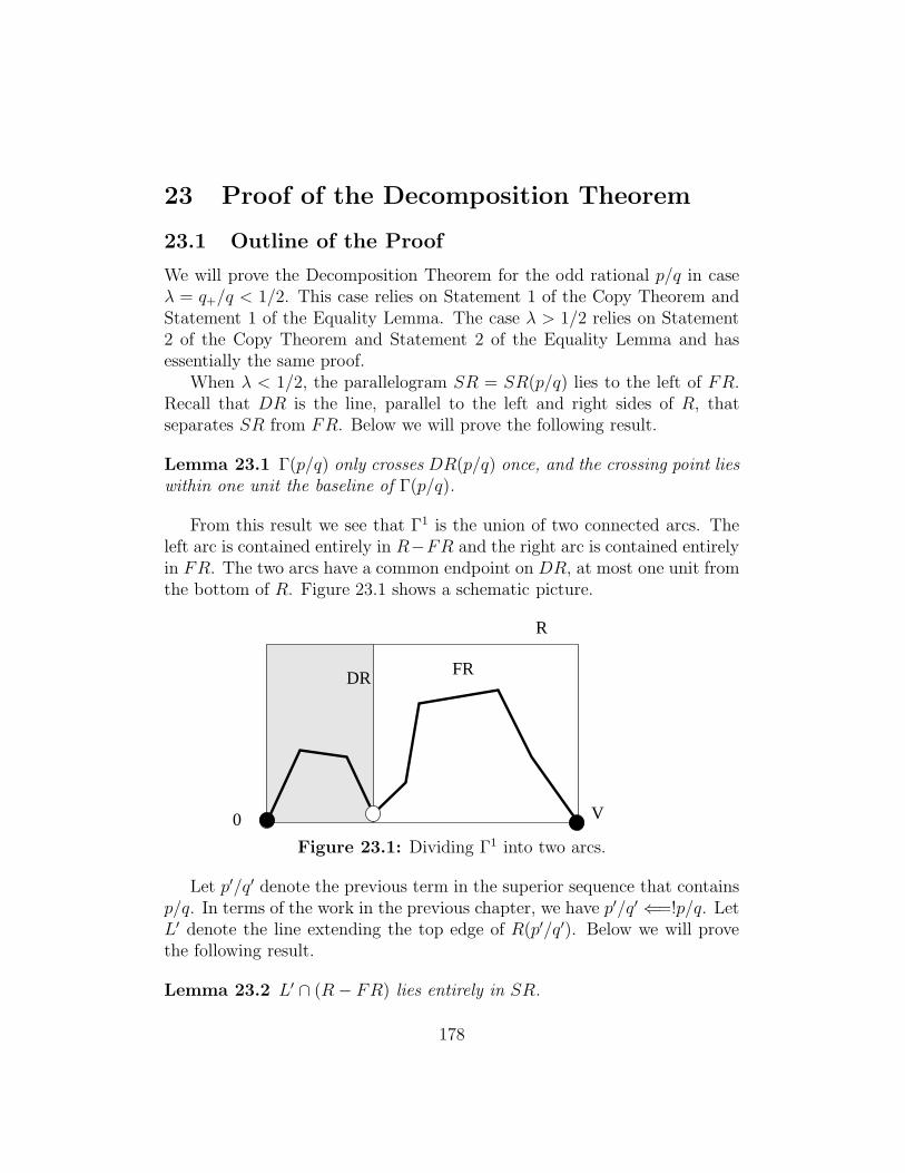
23 Proof of the Decomposition Theorem

23.1 Outline of the Proof

We will prove the Decomposition Theorem for the odd rational p/q in caseλ = q+/q < 1/2. This case relies on Statement 1 of the Copy Theorem andStatement 1 of the Equality Lemma. The case λ > 1/2 relies on Statement2 of the Copy Theorem and Statement 2 of the Equality Lemma and hasessentially the same proof.

When λ < 1/2, the parallelogram SR = SR(p/q) lies to the left of FR.Recall that DR is the line, parallel to the left and right sides of R, thatseparates SR from FR. Below we will prove the following result.

Lemma 23.1 Γ(p/q) only crosses DR(p/q) once, and the crossing point lieswithin one unit the baseline of Γ(p/q).

From this result we see that Γ1 is the union of two connected arcs. Theleft arc is contained entirely in R−FR and the right arc is contained entirelyin FR. The two arcs have a common endpoint on DR, at most one unit fromthe bottom of R. Figure 23.1 shows a schematic picture.

V

FR

R

DR

0

Figure 23.1: Dividing Γ1 into two arcs.

Let p′/q′ denote the previous term in the superior sequence that containsp/q. In terms of the work in the previous chapter, we have p′/q′ ⇐=!p/q. LetL′ denote the line extending the top edge of R(p′/q′). Below we will provethe following result.

Lemma 23.2 L′ ∩ (R− FR) lies entirely in SR.

178

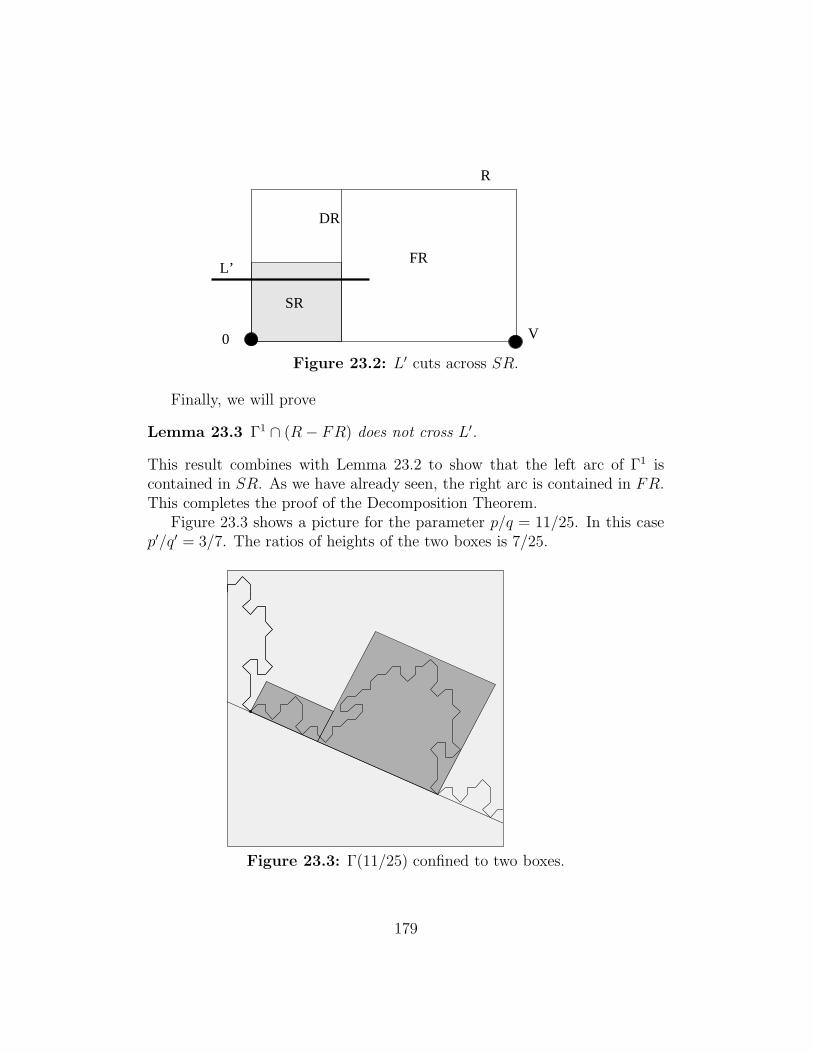
SR

L’

0 V

R

DR

FR

Figure 23.2: L′ cuts across SR.

Finally, we will prove

Lemma 23.3 Γ1 ∩ (R− FR) does not cross L′.

This result combines with Lemma 23.2 to show that the left arc of Γ1 iscontained in SR. As we have already seen, the right arc is contained in FR.This completes the proof of the Decomposition Theorem.

Figure 23.3 shows a picture for the parameter p/q = 11/25. In this casep′/q′ = 3/7. The ratios of heights of the two boxes is 7/25.

Figure 23.3: Γ(11/25) confined to two boxes.

179

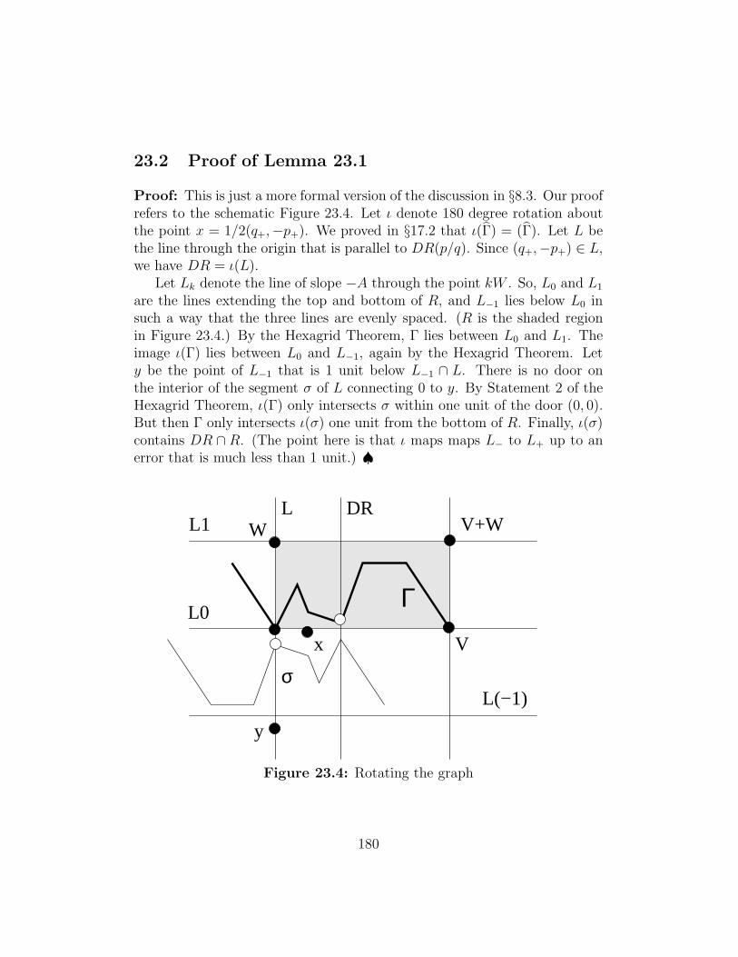
23.2 Proof of Lemma 23.1

Proof: This is just a more formal version of the discussion in §8.3. Our proofrefers to the schematic Figure 23.4. Let ι denote 180 degree rotation aboutthe point x = 1/2(q+,−p+). We proved in §17.2 that ι(Γ) = (Γ). Let L bethe line through the origin that is parallel to DR(p/q). Since (q+,−p+) ∈ L,we have DR = ι(L).

Let Lk denote the line of slope −A through the point kW . So, L0 and L1

are the lines extending the top and bottom of R, and L−1 lies below L0 insuch a way that the three lines are evenly spaced. (R is the shaded regionin Figure 23.4.) By the Hexagrid Theorem, Γ lies between L0 and L1. Theimage ι(Γ) lies between L0 and L−1, again by the Hexagrid Theorem. Lety be the point of L−1 that is 1 unit below L−1 ∩ L. There is no door onthe interior of the segment σ of L connecting 0 to y. By Statement 2 of theHexagrid Theorem, ι(Γ) only intersects σ within one unit of the door (0, 0).But then Γ only intersects ι(σ) one unit from the bottom of R. Finally, ι(σ)contains DR ∩ R. (The point here is that ι maps maps L− to L+ up to anerror that is much less than 1 unit.) ♠

Γ

L(−1)

y

L DR

σ

L1

L0

W

x V

V+W

Figure 23.4: Rotating the graph

180

23.3 Proof of Lemma 23.2

Let L denote the baseline of Γ(p/q). Let L denote the line extending the leftedge of R − FR. Of cource L is also the line extending the left edge of R.Let R denote the line extending the right line of R − FR. Let V ′ and W ′

denote the vectors from Equation 12, defined relative to p′/q′. We will provethree things

1. The distance from L′ ∩ L to W ′ tends to 0 as p′ tends to ∞.

2. L′ ∩ R and L′ ∩ L have the same distance to L, up to an error thatvanishes as p′ tends to ∞.

3. 2‖W ′‖ < ‖W ′‖ − 1/32 once p′ is sufficiently large.

These three properties show that L′ crosses both sides of R − FR beneaththe top left and top right corners of SR. This is what we wanted to prove.

Below, C1, C2, ... refer to universal constants. Let σ stand for slope.

Step 1: L is the line through the origin containing the vector W . We notethat there is a uniformly large angle between adjacent sides of R, independentof parameter. Call this the transversality fact . We have the estimates

|σ(L)−σ(L′)| < C1

K(q′)2; |σ(W )−σ(W ′)| < C2

K(q′)2; ‖W ′‖ < C3q

′. (229)

Comparing the second and third of these estimates, we see that the distancefrom W ′ to L tends to 0 as p′ tends to ∞. Also the difference between theslopes of L and L′ tends to 0 as p′ tends to ∞. From these two properties,and the transversality fact, we see that L′ ∩ L is vanishingly close to W ′.

Step 2: If L and L′ were parallel, then this step would be immediate. Thefirst estimate in Equation 229 shows that the two lines are parallel up toO(K(q′)−2). From the Equality Lemma, we have

width(R− FR) < C2q+ < C3Kq′. (230)

So, the segments of interest to us have length on the order O(Kq′). Thisstep now follows from basic geometry.

181

Step 3: Define

ρ(A) =

√1 + 4A+ 6A2 − 4A3 + A4

2 + 2A∈ [1/2, 1/4]. (231)

From Equation 12 we compute that

‖W‖ = ρ(A)q; ‖W ′‖ = ρ(A′)q′ < ρ(A)(q′ + 1/4). (232)

The last estimate, which holds for p′ sufficiently large, comes from the factthat ρ is lipschitz on [0, 1] and

|A− A′| < 2

(q′)2.

But q ≥ 2q′ + 1. Combining this with Equation 232, we get

‖W ′‖ < ‖W‖2− ρ(A)

4<‖W‖

2− 1

16. (233)

This completes Step 3, as well as our overall proof of Lemma 23.2.

23.4 Proof of Lemma 23.3

Let Γ = Γ(p/q) and Γ′ = Γ(p′/q′). We keep the notatation from the previoussection.

Lemma 23.4 If p′ and p+ are sufficiently large then Γ and Γ′ agree on anyvertex (m,n) that lies within 2 units of X := L′ ∩ (R− FR).

Proof: We define

V+ = (q+,−p+); V− = (q−,−p−). (234)

The endpoints of X are W ′ and V+ +W ′.We will apply the Copy Theorem to p1/q1 = p′/q′ and p2/q2 = p/q. From

Statement 1 of the Equality Lemma, we have

K = 1 +q+q′

; Kq′ = q′ + q+ (235)

182

The point V+ lies vanishingly close to the baseline of Γ(A1). Hence

G′(V+), H ′(V+) ∈ [q+ − 1, q+ + 1] (236)

We also compute

G′(W ′) = − (q′)2

p′ + q′∈∗ [−q′ + 21, 0] ⊂ [−q′ + 20, Kq′ − 20].

H ′(W ′) =(q′)2

p′ + q′∈∗ [0, q′ − 21] ⊂ [−q′ + 20, Kq′ − 20].

HenceG′(V+ +W ′), H ′(V+ +W ′) ∈∗ [−q′ + 20, Kq′ − 20].

The starred containments hold for p′ large enough. The choice of 20comes about because 3 + 2× 8 < 20. The 8 comes From Equation 195.

Our calculations above combine with the gradient bounds in Equation195 so show that (m,n) ∈ ∆(−q′ +3, Kq′−3) provided that (m,n) is within2 units of X. The Copy Theorem now applies. ♠

Applying the Room Lemma to p′/q′, we see that Γ′ does not cross theline L′ at all. By the preceding result, Γ does not cross L′ at any vertex thatlies in R − FR. In short, Γ does not cross L′ ∩ (R − FR). This completesthe proof of Lemma 23.3.

183

24 Proof of Theorem 4.2

24.1 A Consequence of the Copy Theorem

In this section, we deduce a consequence of the Copy Theorem that is tailoredto deal with the inferior sequence constructed in §22. Suppose Am and Am+1

are consecutive terms of an inferior sequence. Lemma 22.2 applies to theseterms. Our next result refers to the various possibilities in Lemma 22.2. Tomake the various cases look as symmetric as possible. We set

λ±m =(qm)±qm

. (237)

This λ+m = λm, as in Lemma 22.2, and λ−m = 1− λm.

Lemma 24.1 Γm and Γm+1 agree on any lattice point (m,n) having theproperty that F1(m,n) > 0 and

G1(m,n), H1(m,n) ∈ [−K−q1 + 3, K+q1 − 3].

Here

1. In Case 1, set K− = 1 and K+ = (κm + 1)/2 + λ+m.

2. In Case 2, set K− = 1 and K+ = (κm + 0)/2 + λ+m.

3. In Case 3, set K+ = 1 and K− = (κm + 1)/2 + λ−m.

4. In Case 4, set K+ = 1 and K− = (κm + 0)/2 + λ−m.

Proof: Consider Case 1 first. Recall that κm = floor(am). Here, as inEquation 192, we have a = a(Am, Am+1). We have κm odd and Am < Am+1.In this case, the fractional part of am/2 lies in [1/2, 1). Referring to the CopyTheorem, we have

K = floor(am/2− λm) + 1 + λm = (κm + 1)/2 + λm.

This fits with what we have written down for Case 1 above.Now Consider Case 1. In this case, the fractional part of κm is less than

1/2 and λm > 1/2. But then

K = floor(am/2− λm) + 1 + λm = (κm + 0)/2 + λm.

This again fits with what we have written down for Case 2 above.Cases 3 and 4 are similar. We omit the details. ♠

184

24.2 Using the Decomposition Theorem

Let Γ = Γ(p/q) be as usual. For the results of this section, we only careabout the portion of Γ above its baseline. We take ǫ = 1/100.

Lemma 24.2 Suppose that Am < Am+1 and κm ≥ 2.

Proof: We either have Case 1 or 2 of Lemma 24.1. In Case 1, we haveκm ≥ 3 odd and λm < 1/2. In this case, we have K− = 1 and K+ = 2. Thisis just like the case n = 1 of Theorem 4.3. The proof there tells us that

Γ1+ǫm ⊂ Γm+1. (238)

Note that qm+1 > 2qm. Hence Vm+1 is more than twice as far from (0, 0) asVm. From this, we see that in fact Γ1+ǫ

m ⊂ Γ1m+1.

In Case 2 we have κm ≥ 2 even and λm > 1/2. Hence, K− = −1 andK+ = 1+λm. This case corresponds to the example in §21.3. Here, a picturesays a thousand words. By the Decomposition Theorem, we have

Γ1m ⊂ FRm ∪ SRm (239)

Since λm > 1/2, the smaller region SRm occurs on the right. This is crucialto our proof. See §21.3.

To apply the Copy Theorem, we need to evaluate G and H on the 4vertices of SRm and the 4 vertices of FRm. For ease of notation, we setSR = SRm, etc. Here is the vertex list, first for FR and then for SR.

0; λW ; V ; V + λW. (240)

λV ; λV +W/2; V ; V +W/2. (241)

Calculations like the ones done in the proof of Theorem 4.2 give us Equation239, and the rest of the proof is as in Case 1. Geometrically, the right verticesof FR sit in the same relation to the right edges of ∆(−q,Kq) as the rightvertices of R sit in relation to ∆(−q, 2q), something we estimated in ourproof of the Theorem 4.2 for n = 1. The critical new calculation here is

H(V +W/2) = q +q2

2(p+ q)∈∗ [0, 3q/2− 3] ⊂ [−q + 3, Kq − 3].

The starred containment holds for p large. The last containment uses thefact that λ > 1/2. Our critical calculation checks that the top right vertexof SR lies inside ∆(−q + 3, Kq − 3). See §21.3. ♠

185

24.3 The End of the Proof

We will prove Theorem 4.2 in the context of two terms pm/qm and pn/qnin the interior sequence, such that κm ≥ 2 and m < n. Any instance ofTheorems 4.2 and 7.5 can be placed in this context. In any case, this is thecontext in which we apply these theorems. We prove Statement 1. The prooffor Statement 2 are essentially the same. Given Lemma 22.6, we just haveto prove that Γ1+ǫ

m ⊂ Γn when n > m+ 1.We will first consider the case n = m+2 in detail. We already know that

Γ1+ǫm ⊂ Γ1

m+1. By Lemma 22.9, the quantity qm+1 − 2qm grows unboundedlywith m. Therefore, Γ1+ǫ

m , which is also a portion of Γm+1, is contained in theunion of two sets:

1. Rm+1/2, the parallelogram obtained by scaling Rm+1 down by a factorof 2 about the origin.

2. The disk of radius qm+1/200 about some point on the bottom edge ofRm+1/2.

In any of the cases of Lemma 24.1, we have K−, K+ ≥ 1. We mean toapply Lemma 24.1 to the pair m+ 1, m+ 2, and vertices in the two sets wehave mentioned. Now we have the same calculation as in the n = 1 caseof Theorem 4.3, except that m + 1 replaces m, and every thing in sight isdivided by 2. Now we know that Γ1+ǫ

m ⊂ Γ1m+2.

Now we can repeat the above argument, with m+ 2 and m + 3 in placeof m+ 1 and m+ 2. That is, Γ1+ǫ

m , which is also contained in Γ1m+2, actually

lies in the union of Rm+2/2 and some disk of radius at most qm+2/200 aboutsome point on the bottom edge of this parallelogram. Running the sameargument as above gives Γ1+ǫ

m ⊂ Γ1m+3. And so on. An induction argument

finishes the proof.

Remark: Even though the Decomposition Theorem only appears once inour argument – in Case 2 of Lemma 24.2 – it plays a crucial role. We couldnot get good enough bounds using just the result from the Room Lemma inthis case. Take another look at the picture in §21.3. The box R1 would stickout of the set ∆ there, and so the Room Lemma itself is not strong enoughto give us what we need. The interested reader can see all these sets usingBilliard King.

186

25 References

[B] P. Boyland, Dual Billiards, twist maps, and impact oscillators , Nonlin-earity 9 (1996) 1411-1438

[De] N .E. J. De Bruijn, Algebraic Theory of Penrose’s Nonperiodic Tilings,Nederl. Akad. Wentensch. Proc. 84 (1981) pp 39-66

[Da] Davenport, The Higher Arithmetic: An Introduction to the Theory ofNumbers, Hutchinson and Company, 1952

[D], R. Douady, These de 3-eme cycle, Universite de Paris 7, 1982

[DF] D. Dolyopyat and B. Fayad, Unbounded orbits for semicircular outerbilliards, preprint (2008)

[DT] F. Dogru and S. Tabachnikov, Dual Billiards , Math Intelligencer vol.27 No. 4 (2005) 18–25

[EV] D. B. A. Epstein and E. Vogt, A Counterexample to the Periodic OrbitConjecture in Codimension 3 , Annals of Math 108 (1978) pp 539-552

[G] D. Genin, Regular and Chaotic Dynamics of Outer Billiards, Penn StatePh.D. thesis (2005)

[GS] E. Gutkin and N. Simanyi, Dual polygonal billiard and necklace dy-namics , Comm. Math. Phys. 143 (1991) 431–450

[Ke] R. Kenyon, Inflationary tilings with a similarity structure, Comment.Math. Helv. 69 (1994) 169–198

[Ko] Kolodziej, The antibilliard outside a polygon, Bull. Polish Acad Sci.Math. 37 (1989) 163–168

[M1] J. Moser, Is the Solar System Stable? , Mathematical Intelligencer, 1978

[M2] J. Moser, Stable and Random Motions in Dynamical Systems, with Spe-cial Emphasis on Celestial Mechanics , Annals of Math Studies 77, Princeton

187

University Press (1973)

[N] B.H. Neumann, Sharing Ham and Eggs,summary of a Manchester Mathematics Colloquium, 25 Jan 1959published in Iota, the Manchester University Mathematics students’ journal

[S] R. E. Schwartz, Unbounded Orbits for Outer Billiards, Journal of ModernDynamics 3 (2007)

[T1] S. Tabachnikov, Geometry and Billiards, A.M.S. Math. AdvancedStudy Semesters (2005)

[T2] S. Tabachnikov, A proof of Culter’s theorem on the existence of pe-riodic orbits in polygonal outer billiards, preprint (2007)

[VS] F. Vivaldi, A. Shaidenko, Global stability of a class of discontinuousdual billiards, Comm. Math. Phys. 110 (1987) 625–640

188