Embed Size (px)
Citation preview
Out in the Sunshine? Outsiders, Insiders and the United States in 1998*
Fabio Ghironi and Francesco Giavazzi
Ghironi: Department of Economics, University of California, Berkeley CA 94720-3880, USA Giavazzi: IGIER, Universita’ Bocconi, via Salasco 3-5, 20136 Milano, Italy
Email: [email protected] and [email protected]
January 1997
Abstract This paper analyzes monetary and fiscal policy interactions in a three-country world, interpreted to represent two EU economies and the rest of the world. The analysis extends well-known results in the literature on international policy spillovers by investigating the effects of different sizes of the two EU economies. A set of general results is derived, which allows a reinterpretation of earlier findings in the literature on policy-making in interdependent economies. JEL Classification: F31, F33, F41, F42 Keywords: international policy coordination, European Monetary Union * The title of this paper was inspired by Spaventa (1996). We thank, for their comments, Matthew Canzoneri, Cedric Dupont, Jürgen von Hagen, Maury Obstfeld and participants in the 1996 KIEL Week Conference, in the Berkeley international macro seminar, and in the Sapir Center Conference on “Optimum Currency Areas.” Althea F. Bickel provided valuable secretarial assistance.
1 Introduction
As the date approaches, when a decision will have to be made on which European states will join the
monetary union from the start, two separate camps are emerging in the countries that are likely
candidates to be admitted to the currency union. On the one side lie the central bankers, mainly
concerned about the credibility and the reputation of the new European central bank (ECB), and
about the extent to which the countries that will adopt the euro will come close to forming an
optimum currency area. On the other side lie industry and the trade unions, mainly worried about
competitiveness, i.e. about the effects that splitting Europe in two separate groups of countries, the
ins and the outs, may have on relative prices inside the European Union (EU.) The sophisticated
argument is that the single market could not survive if exchange rate volatility between the ins and
the outs were high. The unsophisticated argument is that both -- industry and the unions -- are scared
at the prospect of the outs using the exchange rate strategically.
The argument of the central bankers runs as follows. The ECB will not inherit overnight the
reputation of the Bundesbank. For some time it will be carefully watched and tested by the markets
- until it builds its own credibility and reputation. How long will it take for the ECB to achieve this ?
It depends, say the central bankers, on the type of countries that will join the currency union from the
start. If the first group of ins consisted of those countries that already belong to the "Greater D
mark area", building a reputation will not take long -- as the ECB will look very similar to the
Bundesbank since the start. However, as the number of the first group of ins increases, and the
board of the ECB starts speaking more and more languages (and languages that are increasingly
distant from German), building a reputation will take longer and longer. Not only because the
European Council will appoint to the Board of the ECB individuals from states whose anti
inflationary reputation is doubtful, but also, and perhaps more importantly, because the monetary
union will include regions that less and less resemble to an optimum currency area -- thus increasing
the pressures likely to be exerted on the central bank. Hence, conclude the central bankers, let us
start with a small union; this will make it easier for the ECB to build a reputation; once this is
achieved, more countries can be allowed in without prejudice to the new monetary institution which,
by then, will have a strong anti-inflationary reputation of its own.
While the reputation argument is certainly relevant (see de Grauwe 1996, for an analysis)
there are other dimensions to the choice of the optimal size of the currency union. An important one
are the strategic interactions that will take place among the various actors in the EMU game:
between the ECB and the central banks of the outs; between the ECB and the fiscal authorities of the
currency union, i.e. the Ecofin Council; between the central banks of the outs and their own fiscal
authorities; and between these institutions and the rest of the world. (In this paper we think of the
rest of the world as simply the United States, but further work should allow for the growing impact
on Europe of other areas of the world, the Far-east in particular.) For example, following a negative
supply shock, if the outs were able to engineer a real appreciation, thus successfully shifting some of
their inflation upon the ins, the ECB would have a greater incentive to contract its monetary policy
and to export inflation to the U.S. appreciating the euro against the dollar. If the Federal Reserve
reacts by tightening as well, overall these monetary interactions would have negative consequences
for employment both in Europe and in the United States, possibly against the governments'
preferences. (This is the case studied in this paper, but one could think of different situations, such
as, for example, the incentive that the ins may have, whenever they are faced with a loss of
competitiveness relative to the outs, to affect their dollar exchange rate in an attempt to increase
their competitiveness vis-a-vis the United States. In the situation we analyze, it is likely that Ecofin
would put pressure on the ECB towards loosening the monetary contraction by removing the
contractionary bias of non coordinated policies with the Fed. See Ghironi and Eichengreen, 1996, on
this point)
In Europe different policymakers are concerned about different aspects of these strategic
interactions. Those based in the individual states are above all concerned with the consequences of a
division of the EU between ins and outs: thus, the strategic interactions they are interested in are
those that may occur between the authorities of one group of countries and of the other. The
European Commission, instead, works under the assumption that the transition will be short, and that
the EMU will soon include all EU states. What worries the officials in Brussels are the effects on the
international monetary system of the come to stage of a new currency. This paper makes the point
that these two aspects cannot be separated. The interactions between ins and outs cannot be studied
in isolation, since they will be affected by the presence of the rest of the world -- as hinted at in the
example of the previous paragraph. The interactions between EMU and the rest of the world depend,
in turn, on the size of the EMU, and cannot be studied independently of the ins vs. outs question.
This paper brings these two aspects together. We study the incentives that various European
policymakers face in determining the optimal size of the currency union explicitly accounting for the
effects of the interactions inside Europe and between Europe and the rest of the world. We overlook
the ECB credibility problem-- which is well understood-- and ask if there are other reasons why the
central bankers of the likely ins may want to keep the currency union relatively small. At the same
time we ask if the optimal dimension of the union, as seen from the viewpoint of the fiscal
authorities, is different, thus giving rise to a potential conflict between Ecofin and the central bankers
2
at the time of deciding who should join the union. Throughout the paper we discuss how the choices
faced by European policymakers are affected by the presence of the United States (the rest of the
world) and, in tum, how the United States will be affected by the birth of the euro and by the size of
EMU.
The analytical tool we use to address these questions is a 3-country model designed to
describe the interactions among monetary and fiscal authorities, in the tradition of Canzoneri and
Henderson ( 1991.) An attractive feature of the model is that it allows us to study the effects of
different dimensions of the European currency union-- in a continuum that encompasses a currency
union that extends to the entire EU (except perhaps for a few states of negligible magnitude) as well
as one that does not extend beyond Germany and Austria. 1 As common in the literature on the
international spillovers of fiscal and monetary policies, the model is essentially a three-country
version ofthe Mundell-Flerning model, in which the authorities of each region minimize quadratic
loss functions whose parameters differ across different authorities. This particular model has been
first studied in Ghironi ( 1993 ), and used to address different questions in Ghironi and Eichengreen
(1996.)
Inside each region the central bank controls a nominal variable (the money supply or the level
of the exchange rate), while the fiscal authority controls taxes or public spending. The interactions
among different regions occur via trade flows in the goods market, and via capital flows in the assets
markets; we assume that assets are perfect substitutes, so that interest rates and nominal exchange
rates in the three regions are linked through arbitrage conditions. We use the model to study the
response to a common supply shock that hits the three regions simultaneously. The model has two
periods: nominal wages are predetermined and set based on the expectation of future variables
(prices, interest rates, and the policy instruments); the ex-ante return on financial assets also depends
on expected exchange rate changes. However, because the only stochastic factors are exogenous
shocks. whose expectation one-period ahead is equal to zero, the rational expectations solution of
the model (in the absence of time-consistency problems, that we overlook) is straight-forward, since
all expectations are equal to zero; thus the model reduces to a static structure (see also Giavazzi and
Giovannini, 1989, for a similar solution.)
A distinct feature of the model is the assumption about fiscal policy. We rule out debt
accumulation, by imposing that tax revenue equals spending in each period. Government spending
falls on home and foreign goods, according to the same pattern as for private consumption (to be
1 Using a similar framework, von Hagen and Fratianni ( 1991) study a different type of asymmetry -- the effects of asymmetric demand and supply shocks on otherwise symmetric economies.
described later.) We follow Alesina and Tabellini (1987) assuming that government revenue accrues
exclusively from a tax on firms' total revenues, which provides a simple and neat way to capture the
distortionary effects of taxation. Firms' demand for labor is a decreasing function of the tax rate: for
a given level of demand, a tax cut raises employment. This effect, however, is accompanied by the
contemporaneous fall in demand produced by the cut in government spending that must accompany
the tax cut. Hence, the net effect on equilibrium employment remains ambiguous, although for
plausible parameter values the supply effect dominates-- i.e. a tax cut unambiguously raises
employment. (See Giavazzi and Pagano, 1996, for empirical evidence on episodes of expansionary
spending cuts.) The fiscal authority responds to a negative supply shock (which raises prices and
lowers output) by cutting taxes, thus contributing to raise employment and to stabilize the price level
because the tax cut creates excess supply in the goods market.
The trade pattern across the three regions (shown in Figure I) is the novel feature of our
model, which will allows us to compare different sizes of the currency union. We start from the
pattern of transatlantic trade: U.S. consumers spend a fraction (1-h) of total consumption on home
goods, and a fraction h on goods imported from Europe; this in turn is allocated in a fraction a which
falls on goods produced by the ins, and a fraction (f-a) which falls on goods produced by the outs.
European consumers in both regions spend a fraction h on goods imported from the U.S., and a
fraction ( 1-h) on European goods; the latter fraction is distributed in a fraction a which falls on
goods produced by the ins, and a fraction (/-a) which falls on goods produced by the outs2 The
parameter a characterizes the size of the currency union. As a increases, the share of U.S. imports
from Europe that comes from the ins increases, while the import share from the outs falls, thus
describing a situation in which the size of the ins, relative to the outs increases. As a approaches I,
the EU and the ins tend to overlap: the currency union includes all EU states, except for a small
"residual" economy whose actions do not affect the ins and the U.S.; when a falls, the number of
countries in the currency union becomes smaller and smaller.
As mentioned above, there are two authorities in each region: a fiscal authority and a central
bank 3 Each of them minimizes a loss function which includes, as arguments, the fluctuations of
' Our assumptions on the trade pattern are consistent with the implicit assumption that consumers on the two sides of the Atlantic have asymmetric Cobb-Douglas preferences, which lead to constant shares of income being spent on the various goods according to the assumed pattem. ' By doing this we assume that inside the currency union there is a single fiscal authority. represented by the Ecofin Council. This implies two strong assumptions. First. all the members ofthe EU are currently represented in the Ecofin Council: assuming that Ecofin is the fiscal authority of the insiders alone may appear inconsistent with the current institutional framework of the Union. However, officials in Europe are now discussing the possibility of a two-level structure for the Ecofin Council, with the representatives of the insiders constituting the first layer ofthe stmcture. If. for any reason, there is no cooperation between the two subsets, i.e. the two levels, ofEcofin, nothing prevents us from treating them as two separate authorities. with the first layer, to which we simply refer as Ecofin in our paper, being
4
employment and the CPI around their equilibrium values. In addition, the fiscal authorities also care
about the distortions associated with taxation. We shall first consider the case when none of them
cooperates -- neither internationally, nor within the region. The monetary policy regime between the
ins and the United States is symmetric, and, in the absence of international monetary cooperation, it
is subject to the well-known inefficiency associated with flexible exchange rates. Each central bank
controls its own money stock and believes that, by changing it, it can affect the bilateral exchange
rate. Since exchange rates feed back into the domestic CPI, each central bank believes that monetary
policy can affect prices at a relatively smaller cost in terms of output. In the non-cooperative
equilibrium monetary policy turns out to be overly contractionary.
Inside Europe, instead, we study two different monetary regimes. The first is asymmetric: the
central bank of the ins (the ECB) controls its own money stock, but-- contrary to the situation
relative to the dollar -- it is unable to affect the infra-European exchange rate because its partner (the
outs) accommodates any change in the money stock of the ins. Therefore, the ECB minimizes its
loss function subject to the European-wide tradeoff between output and the price level. The central
bank of the outs, instead, controls the bilateral exchange rate. The alternative regime is symmetric,
exactly as we have assumed for the ECB and the Fed.
Which regime will characterize Europe, after EMU is born, is still undecided. Policymakers
(the Commission and the Ecofin Council) are studying a new EMS, linking the single currency with
the currencies ofthe outs: as argued in Giavazzi and Giovannini (1989), we believe that our
asymmetric regime is a good characterization of an EMS-type arrangement where realignments are
non cooperative. The alternative view -- held by the UK authorities and by a number of academic
economists, see in particular Persson and Tabellini ( 1996) -- is that a new EMS would not survive
speculative attacks, especially since the ECB will be unwilling to provide unlimited intervention.
Instead the outs should concentrate on a domestic monetary rule (inflation targeting is the common
proposal) and let the bilateral exchange rate vis-a-vis the euro fluctuate. 4
the fiscal authority of the ins. separated from the fiscal authority of the outs. Second. the first layer itself will include a number of independent fiscal authorities. one for each member of the currency union: we thus overlook the strategic interactions among them. (fhese are studied in Ghironi. 1993. and Ghironi and Eichengreen 1996.) Finally, we also assume that the outs can be aggregated into a single entity, with a single central bank and a single fiscal authority. We therefore overlook the consequences of non-cooperation among the authorities of the outs, studied in Buiter. Corsetti and Pesenti (1996.) 4 Kenen (1995). Spaventa (1996) and Wyplosz (1996). among others, provide a thorough analysis of the arguments in favour and against a new EMS regime between the in.< and the outs. Persson and Tabellini (1996) argue that a regime that combines inflation targeting with flexible exchange rates is strictly superior to an EMS-type regime. They suggest that this regime would approximate the first best cooperative outcome of their model quite closely. removing existing incentives to run competitive devaluations. and would outperform an exchange rate-based regime.
Within this framework we ask whether different authorities (in particular Ecofin and the
ECB), concerned about the consequences of supply-side disturbances, would agree on the desirable
size of the currency union.
In Section 2, we present the model used throughout the paper. In Section 3, we briefly
summarize the general results shown in Ghironi and Giavazzi ( 1997) on how the output-inflation
tradeoff faced by the monetary authority of a region changes, when its relative size, and the
monetary regime that links it to the rest of the world change. These general results provide a
theoretical background for the discussion of the stabilization game in the following sections.
Because some of the reduced form coefficients of the model cannot be signed
unambiguously, we proceed to numerical illustrations of the game for reasonable values of the
parameters. Interestingly, our 3-country model vindicates some of the facts described at the
beginning of this introduction. For example, in a situation where fiscal authorities are prevented
from using the tax instruments (and thus in a situation that closely resembles what could be the
consequences of a strict "fiscal stability pact"), and strategic interactions are limited to those
occurring among central banks in an asymmetric exchange-rate regime (Section 4), the ECB would
prefer the currency union to be rather small if the outs were non negligible; Ecofin, instead, prefers a
situation in which relatively more states join the currency union. In the same section, we compare the
results with those obtained assuming monetary cooperation between the ins and the outs. Section 5
is devoted to the analysis of what happens when fiscal activism is allowed. In Section 6 we start
exploring the importance of the presence of the United States in causing our results by studying what
would happen were the US. and Europe completely closed with respect to one another, i.e. if there
were no transatlantic policy spillovers. We find that the conflict of interests between the ECB and
Ecofin would disappear in this situation. In Section 7, we reintroduce transatlantic policy spillovers
and we compare the results obtained under an asymmetric infra-EU regime with those obtained
assuming a symmetric flexible exchange rate regime between the ins and the outs. The comparison,
which is based on the results about the tradeoffs summarized in Section 3, allows to shed more light
on the policymakers' incentives and on the role of the United States in our analysis.
2 A three-country model of strategic policy interactions
The world is divided into three countries, the United States, the ins, and the outs. The two European
goods are imperfect substitutes for the US. good and for one another. In the absence of disturbances,
Europe and the US. are symmetric to one another. All variables represent deviations of actual values from
6
zero-shock equilibrium values. All variables except interest rates, public expenditures, and tax rates are
expressed in logarithms, and time subscripts are dropped whenever possible.
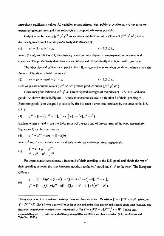
Output in each country (yus, /. fJ ) is an increasing function of employment (nus, d, n° ) and a
decreasing function of a world productivity disturbance (x):
(I) y 1 = (1- a)n1- x, j~US,/,0,
where (I - a.), with 0 < a. < l, the elasticity of output with respect to employment, is the same in all
countries. The productivity disturbance is identically and independently distributed with zero mean.
The labor demand of firms is implicit in the following profit maximization condition, where t indicates
the rate of taxation of total revenues:5
(2) j =liS, I, 0.
Real wages are nominal wages ( wus. W, w0 ) minus product prices (pus. I, p0
).
Consumer price indexes ( qus. q, q0) are weighted averages of the prices of US., ins', and outs'
goods. As shown above in Figure I, American consumers allocate a fraction h of their spending to
European goods (a to the good produced by the ins, and ( 1-a) to that produced by the outs) so the US.
CPI is:
(3) qus =(1-h)pus +ah(t/ +e')+(1-a)h(p" +e').
Exchange rates e1 and e2 are the dollar prices of the euro and of the currency of the fmts, respectively
Equation ( 3) can be rewritten as:
(4) qus=pus+ahz'+(1-a}hz2,
where z1 and:! are the dollar-euro and dollar-mtts real exchange rates, respectively:
(5) z' = e' +PI - p';s,
z' = e' +Po -pus.
European consumers allocate a fraction h of their spending to the U.S. good, and divide the rest of
their spending between the two European goods, a to the ins' good and (I -a) to the outs'. The European
CPls are:
(6) q 1 =a( I- h)p1 + (1- a)(l- hXp 0 + e 2
- e')+ h(pus- e'). q 0 =(1-a)(1-h)p0 +a(1-hXp' +e' -e')+h(p'JS -e2
),
' Using upper-case letters to denote anti-logs. domestic firms maximize Pr ojit = (1 - r )PY - WN . subject to
Y = N'·" /X. Each fim1 is a price taker in the output and in the labor market and is taxed on its total revenues. The
first order condition for maximization with respect toN is (1- r)P(l- a)N-a j X= W. Taking logs.
approximating ln(l --,;)with ..-.. and omitting unimportant constants. we obtain equation (2.) (See Alesina and Tabellini, 1987.)
7
or:
(7) q 1 =p1 -hz'-(1-a)(l-hXz'-z'},
q 0 = p 0 -bz' +a(l-bXz' -z').
The outs-euro real exchange rate is l = z1 - :l.
Demand for all goods increases with output. Residents of each country increase their spending by the
same fraction (0 < E < I) of an increase in output. The marginal propensity to spend is equal to the
average propensity to spend for all goods for residents of all countries. The im' propensity to import from
the outs is ( 1-a) times one minus the ins' propensity to import from the United States. Thus, if the ins'
propensity to import from the U.S. ish, the ins' propensity to import from the outs is (I -a) times (1-h),
and the total propensity to import of the ins is [ h + ( 1-a )( 1-b) ].
An increase in ex ante real interest rates (rus. I, r~ reduces the demand for all goods: residents of
each country decrease spending by the same amount (0 < v < I) for each percentage point increase in the
ex ante real interest rate facing them.
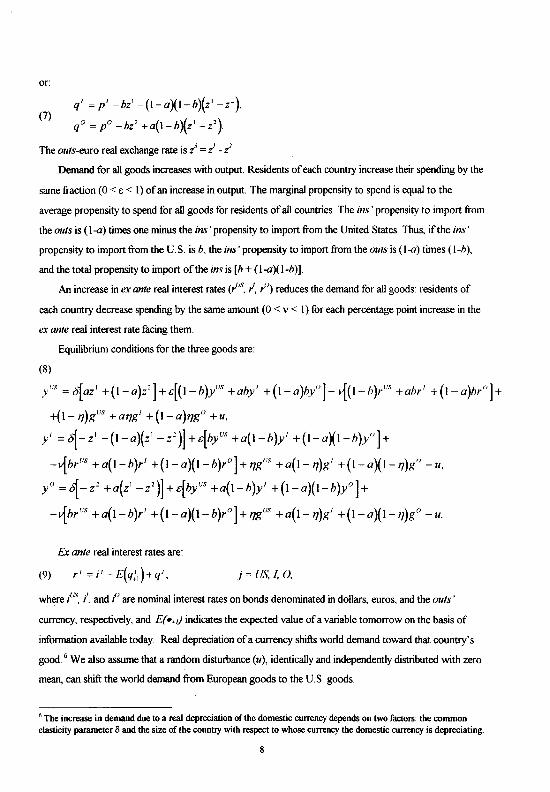
Equilibrium conditions for the three goods are:
(8)
y'1-' = <>1az' +(1-a)z')+c[(t-h)y11
-' +ahy' +(1-a)hy"]- ~(l-h)r'1-' +ahr' +(1-a)hr")+
+(1- '7)g 11s +a'7g1 +(l-a)'lg0 +u,
y' =~-z' -(1-a){z' -z')]+c[hyus +a(l-h)y' +(t-aXl-h)y"]+
-~hrus +a(l-h)r' +(l-a)(l-h)r0 )+'7g'1s +a(l-'l)X' +(1-aXl-'l)x" -u,
y 0 =~-z2 +a{z' -z')]+c(hyus +a(1-h)y' +(l-a)(l-h)y0 )+
-~hrus +a(l-h}r1 +(l-a)(l-b)r0 )+'7gus +a(l-'7)X1 +(1-a)(l-q)g0 -u.
Ex ante real interest rates are:
(9) j = l!S, I, 0,
where ius. I, and P are nominal interest rates on bonds denominated in dollars, euros, and the outs '
currency, respectively, and E( •• ,) indicates the expected value of a variable tomorrow on the basis of
information available today. Real depreciation of a currency shifts world demand toward that country's
good. 6 We also assume that a random disturbance (u), identically and independently distributed with zero
mean, can shift the world demand from European goods to the U.S. goods.
6 The increase in demand due to a real depreciation of the domestic currency depends on two factors: the common elasticity parameter 13 and the size of the country with respect to whose currency the domestic currency is depreciating.
8
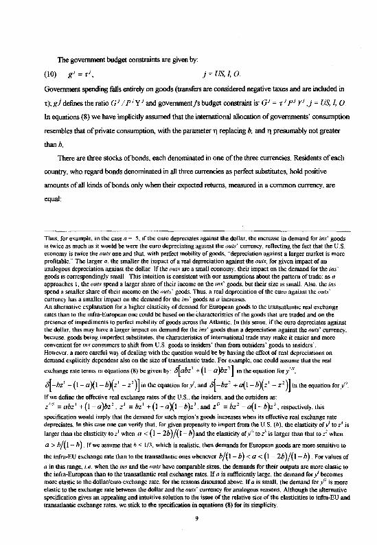
The government budget constraints are given by:
(10) j=US,/,0.
Government spending falls entirely on goods (transfers are considered negative taxes and are included in
t);g) defines the ratio G' I P'Y 1 and govemment/s budget constraint is: G' = r 1 P' Y1 ,j =US, I. 0.
In equations (8) we have implicitly assumed that the international allocation of governments' consumption
resembles that of private consumption, with the parameter 11 replacing b, and 11 presumably not greater
than b.
There are three stocks of bonds. each denominated in one of the three currencies. Residents of each
country. who regard bonds denominated in all three currencies as perfect substitutes, hold positive
amounts of all kinds of bonds only when their expected returns, measured in a common currency, are
equal:
Thus. for example. in the case a= .5. if the euro depreciates against the dollar. the increase in demand for ins' goods is twice as much as it would be were the euro depreciating against the outs' currency. reflecting the fact that the U.S. economy is twice the outs one and that. with perfect mobility of goods. "depreciation against a larger market is more profitable." The larger a. the smaller the impact of a real depreciation against the outs. for given impact of an analogous depreciation against the dollar. If the outs are a small economy. their impact on the demand for the ins' goods is correspondingly small. This intuition is consistent with our assumptions about the pattern of trade: as a approaches I, the outs spend a larger share of their income on the ins' goods, but their size is small. Also. the ins spend a smaller share of their income on the outs' goods. Thus. a real depreciation of the euro against the outs· currency has a smaller impact on the demand for the ins· goods as a increases. An alternative explanation for a higher elasticity of demand for European goods to the transatlantic real exchange rates than to the infra-European one could be based on the characteristics of the goods that are traded and on the presence of impediments to perfect mobility of goods across the Atlantic. In this sense. if the euro depreciates against the dollar, this may have a larger impact on demand for the ins' goods than a depreciation against the outs' currency. because. goods being imperfect substitutes, the characteristics of international trade may make it easier and more convenient for ins consumers to shift from U.S. goods to insiders' than from outsiders' goods to insiders'. However. a more careful way of dealing with the question would be by having the effect of real depreciations on demand explicitly dependent also on the size of transatlantic trade. For example. one could assume that the real
exchange rate terms in equations (8) be given by: 8[ abz 1 + (I -a )bz'] in the equation for y 11
",
o(-bz 1 -{I- aX!- b)(z' - z'))in the equation for/, and o(-bz' +a(l-b)(z' - z')) in the equation fory0
If we define the effective real exchange rates of the U.S .. the insiders. and the outsiders as:
z"" =abz 1 +(1-a)bz'. z 1 = bz' +(1-aXI-b)z' .and z 0 =bz' -a(1-b)z'. respectively. this
specification would imply that the demand for each region's goods increases when its effective real exchange rate depreciates. In this case one can verity that. for given propensity to import from the U.S. (b), the elasticity of/ to:? is
larger than the elasticity to z1 when a< {I- 2b)/(l- b)and the elasticity of/' to z3 is larger than that to z' when
a> h/(1- b). If we assume that b < 1/3. which is realistic. then demands for European goods are more sensitive to
the infra-EU exchange rate than to the transatlantic ones whenever b/(1- b)< a< {I- 2b)/(l- b). For values of
a in this range. i.e. when the ins and the outs have comparable sizes. the demands for their outputs are more elastic to the infra-European than to the transatlantic real exchange rates. If a is sufficiently large, the demand for/ becomes more elastic to the dollar/enro exchange rate. for the reasons discussed above. If a is small. the demand for y" is more elastic to the exchange rate between the dollar and the outs' currency for analogous reasons. Although the alternative specification gives an appealing and intuitive solution to the issue of the relative size of the elasticities to infra-EU and transatlantic exchange rates, we stick to the specification in equations (8) for its simplicity.
9
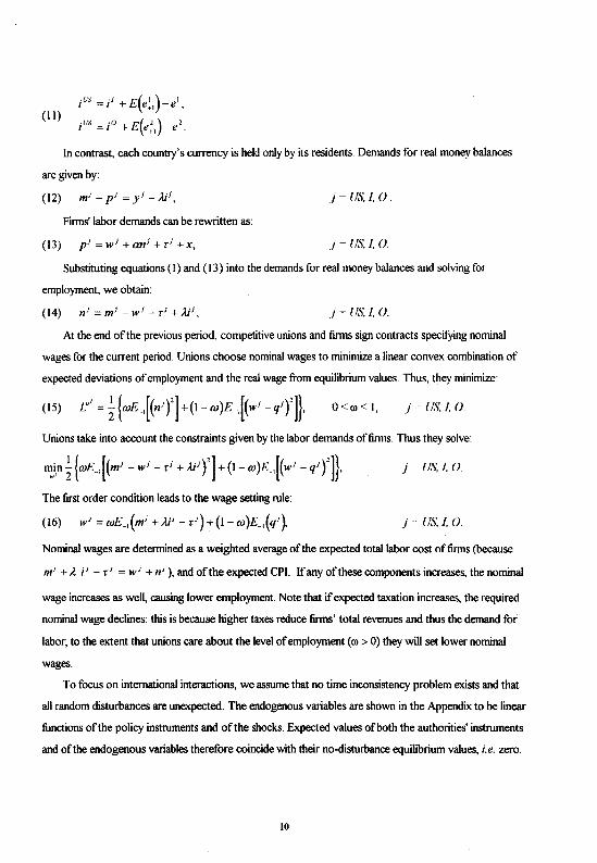
(ll) ius=/ +E(e:,)-e',
ius = i 0 + E(e;,)- e2
In contrast, each country's currency is held only by its residents. Demands for real money balances
are given by:
j~liS,/,0.
Firms' labor demands can be rewritten as:
(13) p; = w; +an; + ,; + x, j~US,/,0.
Substituting equations (I) and (13) into the demands for real money balances and solving for
employment, we obtain:
j ~liS,!, 0.
At the end of the previous period, competitive unions and firms sign contracts specifYing nominal
wages for the current period. Unions choose nominal wages to minimize a linear convex combination of
expected deviations of employment and the real wage from equilibrium values. Thus, they minimize:
O<ro< I, j - US, !, 0
Unions take into account the constraints given by the labor demands of firms. Thus they solve:
The first order condition leads to the wage setting rule:
(16) w1 =wE:_,(m1 +Ai1 --r1)+(1-w)E_,(q1),
.i U.\:1. 0.
j ·• l 1.\: !, 0.
Nominal wages are determined as a weighted average of the expected total labor cost of firms (because
m1 + 2 i 1 - r 1 = w 1 +n1 ), and of the expected CPl. If any of these components increases, the nominal
wage increases as well, causing lower employment. Note that if expected taxation increases, the required
nominal wage declines: this is because higher taxes reduce firms' total revenues and thus the demand for
labor; to the extent that unions care about the level of employment ( ro > 0) they will set lower nominal
wages.
To focus on international interactions, we assume that no time inconsistency problem exists and that
all random disturbances are unexpected. The endogenous variables are shown in the Appendix to be linear
functions of the policy instruments and of the shocks. Expected values ofboth the authorities' instruments
and of the endogenous variables therefore coincide with their no-disturbance equilibrium values, i.e. zero.
10
It will become apparent that zero values for the authorities' instruments are optimal in the absence of
disturbances. 7 Thus the wage setting rule simplifies to:
(17) w' = 0, j=US,/,0.
Plugging this result into the previously obtained expressions for employment and producer prices, we
obtain:
(18) n' = m' - r' + lJ',
(19) p' =an'+ r' + x, j= us./, 0.
Equations (I)-( 19) comprise the structural model. Obtaining reduced fonn expressions requires
tedious algebra, as shown in the Appendix. Here, we simply present the policymakers' preferences and the
main reduced fonn equations.
Each central bank chooses its instrument to minimize:
(20) j =TIS, I, 0.
where y1 measures the weight attached to inflation relative to employment by central banks.
The ECB and the Fed control the respective money supplies, and the exchange rate between the euro and
the dollar is flexible. For the reasons discussed in the introduction, within Europe we compare two
different monetary regimes: (i) an asymmetric regime, in which the ECB sets the money supply, while the
outsiders' central bank sets the value of e' = e 1 - e', the nominal exchange rate between the outsiders'
currency and the euro; (ii) a symmetric regime, in which both the ECB and the outsiders' central bank set
the money supply, and the infra-European exchange rate is floating.
When it plays actively, the government in each country chooses taxes to minimize a quadratic loss
function which depends on the deviations of inflation, employment, and taxation from their equilibrium
values. We assume that the volatility of taxation represents a cost for fiscal authorities. This could be
motivated but the presence of convex distortions, but it could also capture the idea that fiscal policy is
difficult to fine tune relative to monetary policy. 8 Thus, country/ s government minimizes:
When lh is low, the degree of fiscal activism is reduced and the government is forced (e.g by unmodelled
institutional and political constraints) not to use its instrument aggressively in order to act on inflation and
employment. The parameter ~ measures the weight attached to inflation relative to employment by the
7 In Rogotrs (1985) terminology. static expectations are rational. ' Also. volatile taxation could be a source of unfuvourable consequences for politically motivated governments.
II
fiscal authorities. We assume that, in the limiting case lh = 0, in which governments do not play actively,
and taxes are zero, they still care about inflation and employment: their welfare is thus evaluated according
to the criterion:
j ~ us: I, 0.
Once reduced form equations for interest rates and exchange rates are obtained, we see that
endogenous variables in each country are linear functions of the policy instruments and of the
disturbances. This implies that when x = u = 0, zero values of the instruments ensure zero losses for all
authorities, and proves the rationality of static expectations under the assumption that disturbances have
zero mean.
We next show the reduced form equations for employment and the CPI in each country, in the two
European monetary regimes. In the equations that follow, all parameters indexed by a number are
functions of a, the parameter which defines the size of the currency union. When a < I, reduced fonns for
employment in the three countries are :
(i) managed exchange rates inside Europe :
nus =Am us- ilrus- 0m1 + '1'1 r 1 + '1'
2 r"- ~,e' + Ku- H.x,
(23) 111 = Am1
- n, r 1 + n, r 0- emus+ 'l'r 11
"' + ~,e'- Ku- H.x,
n° = Am1 -il3r 0 +il4 r 1 -0m"s + 'l'r"s + ~,e'- Ku- H.x;
and the following relations hold among the reduced form parameters:
'F, + 'F, = r. -n, +fl, = -n, +fl.= -n: (ii) jlexih/e exchange rates in~ide Europe :
n"s = Amus - n ,us - 01m1
- 02m0 + '¥, r 1 + '1', r0 + Ku- Hx,
(23') n 1 = A 1m1 +A
2m0 -!l1r 1 +il2 r 0 -0m"s + 'l'rus -Ku-H.x,
n° = A3m0 + A 4m1 -il3 r 0 +il4 r 1
- 0m"s + 'l'rus- Ku- H.x;
and the following relations hold among the reduced form parameters:
0,+02 =0, '1',+'1',='1', A,+A 2 =A 3 +A4 =A, -il,+il2 =-il,+il4 =-il. 9.
When a= I the outsiders are a "small open economy" which is affected by the U.S. and the insiders'
policies but whose choices have no effect abroad; equations (23) and (23 ') reduce to:
"The expression is further simplified when a= .5, in which case the two European countries are symmetric in each
respect. In this case we have: 0 1 = 0 2 = 0/2, '1'1 = '¥2 = '1'/2. U.S. variables depend on U.S. policy
instruments and on the arithmetic .average of the Enropean ones -and also:
A,= A,, A2 =A4 , n, =il3 , il2 =il4 •
12
(i) managed exchange rates inside Europe:
nus = Am us _ !l-rus _ emJ +'I' 'I"J + Ku _ Hx,
(24) n1 = Am1 -!l-r1 -emus +'l'-r11s -Ku-Hx,
n° = Am1 - n, '1"
0 + n. '1"1 -em"$ + '1'-rus + ~,e' - Ku- Hx.
(ii).flexible exchange rates inside Europe:
nus = Amus- !l-rus- emJ + '1'-rJ + Ku- Hx,
(24') n1 = Am1 - !l -r 1 -emus +'I' -r 11s - Ku- Hx,
n° = A 3m0 + A 4m
1- !l3 -r 0 +!l4 -r 1 -emus+ 'l'-r115
- Ku- Hx.
Similarly, when a< 1, reduced forms for the CPis' are:
(i) managed exchange rates imide ""-urope:
q"s =An/'S- Bm1 + Er"s + r, r' + r1r 0- M,e' + ct>u +LX,
(25) q' =Am'- Bm':s + E,r' + E,r" + fr 11s- M2e 3- ct>u+ Lx,
q 0 =Am' - Bmr:s + E2 -r 0 + E,-r' + fz-'1.< + M.,e'- ct>u +:Ex;
and r, + r 2 = r, E I + E 2 = E . Note that the insiders' fiscal policy has the same impact on both the
insiders' and the outsiders' CPis', and the same is true for the outsiders' fiscal policy. This can be seen
observing that, subtracting q0 from c/, one obtains: q- q0 = -(M2 + M3)e
3, independent oft. Recalling
the expressions for{/ and c/ in terms ofPPis' and real exchange rates (equations (7)) and using the
definitions ofz1 and i, it is possible to show that it actually has to be the case that q- q0 =- e3, i.e. that it
has to be M2 + M, = 110
{i!) .flexible exchange rates inside Europe:
q'!S = Am11s - B,m1 - B1m0 + Er[!S + r, r1 + r2 r 0 + ct>u + Lx,
(25') q' = A,m' - A1m0- Bm'JS + E, r 1 + E 2 r
0 + fr"s - ct>u +:Ex,
q 0 = A3m0
- A4m1
- Bmus + E3 r 0 + E4 r
1 + frus - ct>u +:Ex;
'"This is because the two European countries have identical consumption bundles (see the pattern of trade), and therefore Purchasing Power Parit)' (PPP) holds in terms of CPis. The same is not true for the U.S. versus European economies. because the consumption baskets are asynunetric across the Atlantic. This is due to our implicit assumption that consumers on the two sides of the Atlantic have asynunetric Cobb-Douglas preferences (recall footnote 2.)
13
and B, + B, = B. T, + £; = r. A, - A, = A, - A4 = A, E, + E, = E, + E 4 = E . 11 As a
consequence of the change in the infra-European exchange rate regime, it is no longer the case that the
insiders' fiscal policy has the same impact on both the insiders' and the outsiders' CPI's, and that the same
holds for the outsiders' fiscal policy.
If the outsiders are vel)' small (a= 1), the previous reduced form equations become:
(i) managed exchange rates inside Europe:
qus = Amus -Bmi +Erus +fri +<l>u+:Ex,
(26) qi = Ami - Bmus + E 'i + r ,us - <l>u + :Ex,
q0 =Ami - Bmus + Eri + r,us +e 3- <l>u+ :Ex.
Note that, while the outsiders' fiscal policy still affects tP when a= I, it no longer affects l. Also, in this
situation, movements of e3 have a one-to-one impact on the insiders' CPl."
(ii) flexible exchange rates inside Europe:
qf!S = Am us - Bm1 + E ,u.< + r <1 + <l>u + :Ex,
(26') q 1 = Am1 - Bm11s + Er- 1 + r,us- <l>u +:Ex,
q" = A3m0
- A 4m1- Bmus + E3r 0 + E
4r 1 + r,us- <1>11 +:Ex.
When the European exchange rate regime is symmetric, it is no longer the case that the outsiders' fiscal
policy has no impact on q0 when the outsiders are vel)' small.
The reduced form parameters in the preceding equations are functions of the structural parameters.
Their signs are often ambiguous, since they depend on the interaction of several channels of transmission.
In equations (23, 23')-(26, 26') all the coefficients are assumed to be positive; the signs are those implied
by our assumptions on the value of the structural parameters, which are chosen in order to provide
clearcut conclusions in the response to a supply shock. Recall also that the values of the reduced form
parameters which are not indexed by a number do not change as a does, for given values of the other
structural parameters of the model. 0
11 Again. matters are simpler when a=.5. in which case we have:
B, = B, = B / 2,T, = £; = r / 2,A, = A,,A1 = A,,E, = E 1 .• E 3 = E 4 •
1 2 This is a consequence of the outsiders' consumption pattern: in the case a = I, the outsiders consume only the U.S. and the
insiders' goods. The outsiders' CPI can be rewritten as q 0 = p 0 + (I - h )z 1 - z 2
. Using z 2 = e 2 + p 0 - pus and
the definition ofe3• q0 becornes: q0 = (1- b)z' - e' + e 3 +pus. This equation shows the one-t<H>ne impactofe3 onq"
and proves that the latter is leftunaffi:cted by changes in the outsiders' fiscal policy, asz'. e1, andp1
;s do not depend on the outsiders' policy instruments. 13 Moreover, the par.uneteJS whose value does not depend on a are identical across infra-European exchange rate regimes, as our choice of notation indicates. The intuitioa for tbis n:sult is apparent if one obsetves the n:duced form equations fur the case a =1. The parameters we are rdCning to are indeedtbosethat wouldcllarncrerize the inleraction bctweaHhe U.S. and a
14
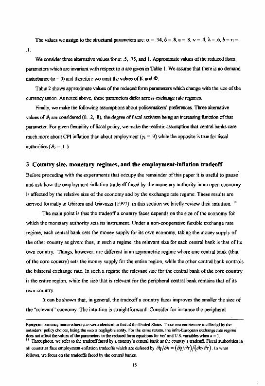
The values we assign to the structural parameters are: a= .34, li = .8, e = .8, v = .4, A.= .6, b = 11 =
.I.
We consider three alternative values for a: .5, . 75, and l. Approximate values of the reduced form
parameters which are invariant with respect to a are given in Table l. We assume that there is no demand
disturbance (u = 0) and therefore we omit the values ofK and ell.
Table 2 shows approximate values of the reduced form parameters which change with the size of the
currency union. As noted above, these parameters differ across exchange rate regimes.
Finally, we make the following assumptions about policymakers' preferences. Three alternative
values of fJ, are considered (0, .2, .8), the degree of fiscal activism being an increasing function of that
parameter. For given flexibility of fiscal policy, we make the realistic assumption that central banks care
much more about CPI inflation than about employment (YI = . 9) while the opposite is true for fiscal
authorities ( fh = . I . )
3 Country size, monetary regimes, and tbe employment-inflation tradeoff
Before proceding with the experiments that occupy the remainder of this paper it is useful to pause
and ask how the employment-inflation tradeoff faced by the monetary authority in an open economy
is affected by the relative size of the economy and by the exchange rate regime·. These results are
derived formally in Ghironi and Giavazzi ( 1997): in this section we briefly review their intuition. 14
The main point is that the tradeoff a country faces depends on the size of the economy for
which the monetary authority sets its instrument. Under a non-cooperative flexible exchange rate
regime, each central bank sets the money supply for its own economy, taking the money supply of
the other country as given; thus, in such a regime, the relevant size for each central bank is that of its
own country. Things, however, are different in an asymmetric regime where one central bank (that
of the core country) sets the money supply for the entire region, while the other central bank controls
the bilateral exchange rate. In such a regime the relevant size for the central bank of the core country
is the entire region, while the size that is relevant for the peripheral central bank remains that of its
own country.
It can be shown that, in general, the tradeoff a country faces improves the smaller the size of
the "relevant" economy. The intuition is straightforward. Consider for instance the peripheral
European currency union whose size were identical to that of the United States. These two entities are unaffected by the outsiders' policy choices, being the outs a neglig.ble entity. For the same reason, the infta-European exchange rate regime does not affect the values of the parameters in the reduced fonn equations for ins' and U.S. variables when a= I. 14 Throughout, we refer to the tradeoff faced by a country's central bank as the country's tradeoff. Fiscal authorities in
all countries face employment -inflation tradeoffs which are defined by cq I m = ( cq I iJr) I ( m I iJr) . In what
follows, we focus on the tradeoffs faced by the central banks.
15
country in an asymmetric regime. The smaller the economy, the larger the share of imports in the
domestic CPl. Thus the impact of a given change in the exchange rate on the CPI increases as the
size of the economy gets smaller-- and thus it becomes more open. A small, open economy therefore
needs to engineer a relatively milder recession to stabilize prices, compared to a large country where
the exchange rate has only a small impact on the domestic CPl.
This result has two corolloraries. Consider, first, the following comparison: the central bank
of a peripheral country in an asymmetric regime, and the same central bank in a symmetric flexible
exchange rate regime. The size of the relevant economy is the same in the two situations-- and thus
the tradeoff the central bank faces is also identical in the two regimes. This is not true, however, for
the central bank of the core country in an asymmetric regime, compared with the situation under
flexible exchange rates. The tradeoff this central bank faces is always less favourable in the
asymmetric regime, when the relevant economy encompasses the entire region, and the two tradeoffs
coincide when the size of the peripheral country becomes negligible-- the Federal Reserve is
indifferent between a regime of fixed or flexible exchange rates vis-a-vis Grenada, but it clearly cares
about the exchange rate regime vis-a-vis Germany or Japan.
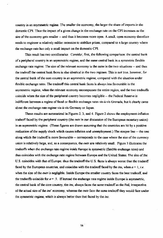
These results are summarized in Figures 2, 3, and 4. Figure 2 shows the employment-inflation
tradeoff faced by the peripheral country (the outs in our discussion of the European monetary union)
in an asymmetric regime. (These figures are drawn assuming that the countries are hit by a positive
realization of the supply shock which causes inflation and unemployment.) The steeper line-- the one
along which the tradeoffls more favourable-- corresponds to the case where the size of the currency
union is relatively large, and, as a consequence, the outs are relatively smaU. Figure 3 illustrates the
tradeoff's when the exchange rate regime inside Europe is symmetric (flexible exchange rates) and
thus~incides with the exchange rate regime between Europe and the United States. The size of the
U.S. coincides with that of Europe: thus the tradeoff the U.S. faces is always worse than the tradeoff
faced by the European countries, and coincides with the tradeoff faced by the ins, when a= I, i.e.
when the size of the outs is negligible. Inside Europe the smaller country faces the best tradeoff, and
the tradeoffs coincide for a= .5. If instead the exchange rate regime inside Europe is asymmetric,
the central bank of the core country, the ins, always faces the same tradeoff as the Fed, irrespective
of the actual size of the ins' economy, whereas the outs face the same tradeoff they would face under
the symmetric regime, which is always better than that faced by the ins.
t6
4 Monetary policy interactions between the ins, the outs, and the United States
The general results stop with those discussed in the previous section -- and this is not surprising.
Remember that what we are looking for are situations in which some policymakers prefer a relatively
larger currency union, while others prefer a relatively smaller one, but all policymakers minimize
employment and price-level fluctuations, albeit with different weights. If it turned out that a given
size of the currency union was best independently of parameter values, then policymakers would
never disagree. Therefore what we are going to show are situations in which, for instance, the
policymakers that give a larger weight to price-level, relative to employment fluctuations, prefer, say
a relatively smaller union, while the opposite holds for policymakers with different relative weights.
Our first exercise only considers monetary policy interactions; we thus assume that the tax
rate ( t) is held exogenously constant -- for instance because of an institutional constraint on the
active use of fiscal policy. The three fiscal authorities passively watch the interactions among central
banks, and their loss functions only include the employment and CPI terms, as in equation (22.) The
three central banks do not cooperate, and the infra-EU exchange rate system is asymmetric.
We believe that this is a good characterization of the way EMU might work, at least for some
time. The "fiscal stability pact", if approved, will tie the hands of the fiscal authorities of the ins,
while the efforts to meet the Maastricht deficit criteria will in tum prevent the outs from actively
using fiscal policy to respond to shocks. The desire of reducing the U.S. public debt may motivate
inaction by the U.S. government. The assumption that monetary authorities do not cooperate is also
a serious possibility. The ECB was designed to be independent; even if a new EMS-type
arrangement is introduced, linking the currencies of the ins and the outs, it is unlikely that the ECB
would deviate from its objectives in order to support the currencies of the outs. As a consequence,
the latter central banks could use the exchange rate strategically in the attempt to shift upon the ins
some of the cost of adjusting. to exogenous shocks -- precisely as in the m~aged exchange rate
regime described in the introduction.
Within this institutional framework we ask what incentives will drive European policymakers
at the time of deciding how many states should be admitted into the currency union. Although
formally this decision is the responsibility of the European Council on a recommendation by Ecofin,
central bankers (the EMI at that stage, since the ECB will not yet be born) will be very influential.
(The European Council will decide based on a recommendation by Ecofin, which in turn will receive .
two reports, one from the EMI, and one from the European Commission.) We would like to know if
the two bodies, Ecofin and the EMI, will have different views, and what determines such
17
differences. 15 More precisely, we ask the following question: for a given policy regime-- no
cooperation among central banks, monetary policy asymmetry inside Europe and frozen fiscal policy
-- following an exogenous supply shock, how large a currency union would each authority prefer,
i.e. how does the loss function of each authority change, as the parameter a changes ?
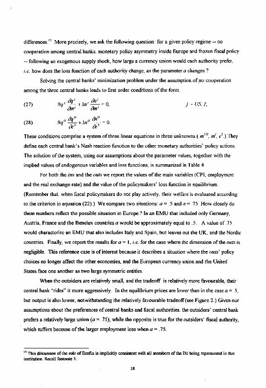
Solving the central banks' minimization problem under the assumption of no cooperation
among the three central banks leads to first order conditions of the form:
(27)
(28)
J'ln) . ml .9q 1 _"'1 __ +.1n1 -- = 0 an) an) '
0 i1J 0 0 roO
.9q --3
+.in --, = 0. a a
j ·~ liS./;
These conditions comprise a system of three linear equations in three unknowns ( mus. ITI, e3) They
define each central bank's Nash reaction function to the other monetary authorities' policy actions.
The solution of the system, using our assumptions about the parameter values, together with the
implied values of endogenous variables and loss functions, is summarized in Table 4.
For both the ins and the outs we report the values of the main variables (CPI, employment
and the real exchange rate) and the value of the policymakers' loss function in equilibrium.
(Remember that, when fiscal policymakers do not play actively, their welfare is evaluated according
to the criterion in equation (22).) We compare two situations: a= .5 and a= .75. How closely do
these numbers reflect the possible situation in Europe ? In an EMU that included only Germany,
Austria, France and the Benelux countries a would be approximately equal to .5. A value of .75
would characterize an EMU that also includes Italy and Spain, but 1eaves out the UK, and the Nordic
countries. Finally, we report the results for a= I, i.e. for the case where the dimension of the outs is
negligible. This reference case is of interest because it describes a situation where the outs' policy
choices no longer affect the other economies, and the European currency union and the United
States face one another as two large symmetric entities.
When the outsiders are relatively small, and the tradeoff is relatively more favourable, their
central bank "rides" it more aggressively. In the equilibrium prices are lower than in the case a= .5,
but output is also lower, notwithstanding the relatively favourable tradeoff(see Figure 2.) Given our
assumptions about the preferences of central banks and fiscal authorities, the outsiders' central bank
prefers a relatively large union (a= . 75), while the opposite is true for the outsiders' fiscal authority,
which suffers because of the larger employment loss when a=. 75.
1' This discussion of the role of Ecofin is implicitly consistent with all members of the EU being represented in that
institution. Recall footnote 3.
18
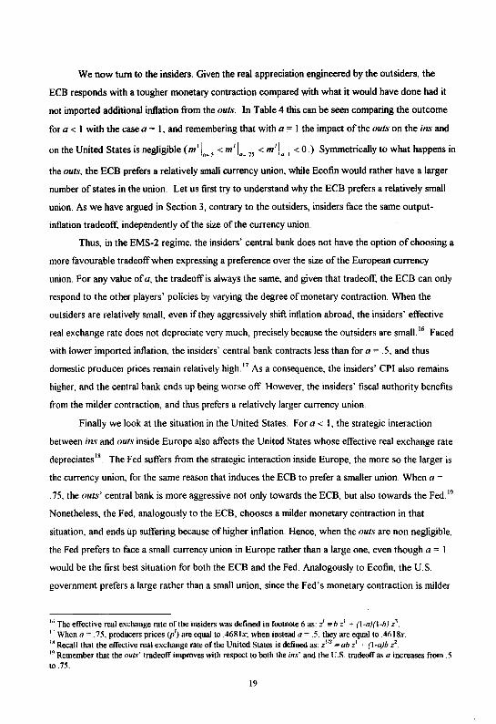
We now turn to the insiders. Given the real appreciation engineered by the outsiders, the
ECB responds with a tougher monetary contraction compared with what it would have done had it
not imported additional inflation from the outs. In Table 4 this can be seen comparing the outcome
for a < I with the case a = 1, and remembering that with a = I the impact of the outs on the ins and
on the United States is negligible ( m1 1.~ 5
< m1 1.= 75
< m1 1.=1
< 0.) Symmetrically to what happens in
the outs, the ECB prefers a relatively small currency union, while Ecofin would rather have a larger
number of states in the union. Let us first try to understand why the ECB prefers a relatively small
union. As we have argued in Section 3, contrary to the outsiders, insiders face the same output
inflation tradeoff, independently of the size of the currency union.
Thus, in the EMS-2 regime, the insiders' central bank does not have the option of choosing a
more favourable tradeoff when expressing a preference over the size of the European currency
union. For any value of a, the tradeoff is always the same, and given that tradeoff, the ECB can only
respond to the other players' policies by varying the degree of monetary contraction. When the
outsiders are relatively small, even if they aggressively shift inflation abroad, the insiders' effective
real exchange rate does not depreciate very much, precisely because the outsiders are small. 16 Faced
with lower imported inflation, the insiders' central bank contracts less than for a= .5, and thus
domestic producer prices remain relatively high. 17 As a consequence, the insiders' CPI also remains
higher, and the central bank ends up being worse off. However, the insiders' fiscal authority benefits
from the milder contraction, and thus prefers a relatively larger currency union.
Finally we look at the situation in the United States. For a < 1, the strategic interaction
between ins and outs inside Europe also affects the United States whose effective real exchange rate
depreciates18 The Fed suffers from the strategic interaction inside Europe, the more so the larger is
the currency union, for the same reason that induces the ECB to prefer a smaller union. When a =
. 75, the outs' central bank is more aggressive not only towards the ECB, but also towards the Fed. 19
Nonetheless, the Fed, analogously to the ECB, chooses a milder monetary contraction in that
situation, and ends up suffering because of higher inflation. Hence, when the outs are non negligible,
the Fed prefers to face a small currency union in Europe rather than a large one, even though a= I
would be the first best situation for both the ECB and the Fed. Analogously to Ecofin, the U.S.
government prefers a large rather than a small union, since the Fed's monetary contraction is milder
1" The effective real exchange rate of the insiders was defined in footnote 6 as: z' =b z1
+ (1-a}(l-b) z'. 1' When a= .75. producers prices (p1
) are equal to .468lx: when instead a= .5. they are equal to .4618x. "Recall that the effective real exchange rate of the United States is defined as: z'IS =ab z1 + (1-a)b .?. 19 Remember that the outs' tradeoff improves with respect to both the ins' and the U.S. tradeoff as a increases from .5 to .75.
19

in the former case and the employment loss is smaller. Note that both the ins and the U.S. face the
same employment-inflation tradeoff as a consequence of the exchange rate regime in Europe, which
presents the ins' authorities with the European-wide tradeoff, independently of the size of the
currency union. Consequently, the presence of non negligible outsiders-- and the absence of infra
European monetary cooperation, as we shall see below-- is crucial to have movements in the dollar
euro exchange rate in the framework we are examining. In fact, if the outsiders were negligible-- or
if they were non negligible but cross-country externalities in Europe were internalized-- equal
tradeoffs would lead to equal equilibrium policies in the U.S. and in the currency union and there
would be no changes in the dollar-euro exchange rate 20
The results presented in Table 4 allow us also to make an interesting comparison with the
analysis of Alesina and Grilli (1994.) There the authors show that if EMU does not include all EU
central banks from the start and monetary authorities in Europe have different degrees of inflation
aversion, it may be the case that the initial insiders will not want the number of the ins to increase,
even if a currency union encompassing all EU members would be the first best.
Something analogous happens in our model. If we think of the three values of a that we have
considered as steps towards global monetary unification of Europe, if initially a= .5, subsequently,
the ECB will not want to take the intermediate step towards a= . 75, even if a - I would be the first
best solution. Interestingly, the Fed would share the ECB's preferences, and-- in a sense-
shortsightedness, contrary to the respective governments, which would always prefer a large
currency union in Europe. We remark that we obtain the Alesina-Grilli result in a framework in
which all central bankers have the same inflation aversion throughout the world. In our view, this
shows that strategic interactions per se may matter at least as much as different degrees of inflation
aversion in shaping policymakers' incentives and behaviour.
How do these results compare with the case of cooperation among central banks in Europe "
We study this case because, according to some officials (but also according to Spaventa, 1996), the
exchange rate arrangement that should link the ins and the outs after January 1", 1999 (the EMS-2)
will entail -- contrary to our assumption so far -- some form of cooperation between the ECB and
'" This observation shows that facing a more favourable tradeoff is not necessa~v in order to successfully run beggarthy-neighbour policies: the Fed faces the same tradeoff as the ECB, but still manages to appreciate the dollar in real terms against the euro, thus ex")Xlrting some inflation to the currency union. The absence of infra-EU cooperation and the presence of non negligible outsiders which successfully export inflation to both the ins and the U.S. shifts the balance between the Fed and the ECB in a direction that is favourable to the U.S. authority. Ghironi ( 1993) and Ghironi and Eichengreen ( 1996) show that the dollar-euro exchange rate would move also in a situation in which there are no outsiders-- so that the currency union has the same size as the U.S. -but fiscal authorities inside the currency union do not cooperate.
20
the central banks of the countries that will not join the currency union from the start. Their
interpretation of how the new system could work is that of a cooperative managed exchange rate
system. The response of EU central banks to exogenous shocks would entail a EU wide change in
the money supply, and, possibly, a cooperative realignment ofinfra-EU exchange rates.
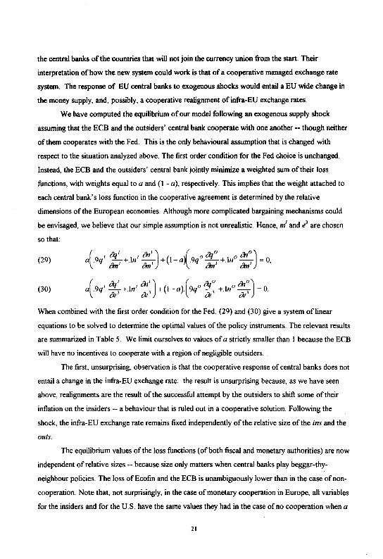
We have computed the equilibrium of our model following an exogenous supply shock
assuming that the ECB and the outsiders' central bank cooperate with one another -- though neither
of them cooperates with the Fed. This is the only behavioural assumption that is changed with
respect to the situation analyzed above. The first order condition for the Fed choice is unchanged.
Instead, the ECB and the outsiders' central bank jointly minimize a weighted sum oftheir loss
functions, with weights equal to a and (1 -a), respectively. This implies that the weight attached to
each central bank's loss function in the cooperative agreement is determined by the relative
dimensions of the European economies. Although more complicated bargaining mechanisms could
be envisaged, we believe that our simple assumption is not unrealistic. Hence, ,/ and e3 are chosen
so that:
( , ilf' , a11
) ( 0 ilf0
0 m0
) (29) a .9q an' +.In an' +(1-a) .9q an1 +.In an' = 0,
(30) a( 9q' z: +.In' ~:) + (1-a).( 9q" z: +.In° ~:) = 0.
When combined with the first order condition for the Fed, (29) and (30) give a system oflinear
equations to be solved to determine the optimal values of the policy instruments. The relevant results
are summarized in Table 5. We limit ourselves to values of a strictly smaller than I because the ECB
will have no incentives to cooperate with a region of negligible outsiders.
The first, unsurprising, observation is that the cooperative response of central banks does not
entail a change in the infra-EU exchange rate: the result is unsurprising because, as we have seen
above, realignments are the result of the successful attempt by the outsiders to shift some of their
inflation on the insiders -- a behaviour that is ruled out in a cooperative solution. Following the
shock, the infra-EU exchange rate remains fixed independently of the relative size of the ins and the
outs.
The equilibrium values of the loss functions (ofboth fiscal and monetary authorities) are now
independent of relative sizes-- because size only matters when central banks play beggar-thy
neighbour policies. The loss ofEcofin and the ECB is unambiguously lower than in the case of non
cooperation. Note that, not surprisingly, in the case of monetary cooperation in Europe, all variables
for the insiders and for the U.S. have the same values they had in the case of no cooperation when a
21
= l, so that monetary cooperation between ins and outs is equivalent to no cooperation when a= I
from the perspective of the U.S. and of the ins. The ECB's gain from cooperation increases as the
size of the union increases, where the gain is defined as the difference between the loss in the absence
of cooperation and the loss under the cooperative EMS-2 regime. This result is intuitive: as we have
argued above, smaller outsiders are more aggressive, and this makes the potential gains for the ECB
from cooperating with the outs' central bank larger.
The situation, however, is different for the outsiders. The outsiders' central bank is better off
in the absence of cooperation -- the more so the larger is the currency union -- because it is then
allowed to appreciate vis-a-vis the insiders. (This is also true when the size of the outsiders is
negligible (a= 1).)21 The outsiders' government, instead, always prefers monetary cooperation in
Europe because it benefits from less contractionary monetary policies. Finally, monetary
cooperation inside Europe benefits the Fed and the U.S. government-- because infra-European
cooperation removes the more aggressive behaviour by the outs' central bank, which induced a real
depreciation of the dollar against the outsiders' currency, and alleviates the deflationary bias
associated with the lack of monetary cooperation in Europe.
5 The interplay of monetary and fiscal policy interactions
As we have argued, the results obtained assuming that the fiscal authorities passively watch the
interactions among central bankers characterize a currency union accompanied by a very tight "tiscal
stability pact" that de-facto prevents governments from using their fiscal instruments. In such a
situation we have shown that a disagreement between the Ecofin Council and the central bankers on
the optimal size ofthe union may arise simply as a result of the lack of cooperation among EU
monetary authorities, and thus quite independently of the consideration that-- at least for some time
-- the ECB could be more credible in a relatively smaller and more homogeneous union.
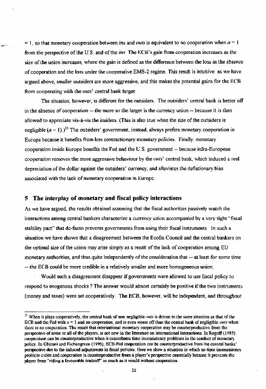
Would such a disagreement disappear if governments were allowed to use fiscal policy to
respond to exogenous shocks? The answer would almost certainly be positive if the two instruments
(money and taxes) were set cooperatively. The ECB, however, will be independent, and throughout
01 When it plays cooperatively, the central bank of non negligible outs is driven to the same situation as that of the ECB and the Fed with a = I and no cooperation, and is even worse off than the central bank of negligible outs when there is no cooperation. The result that international monetary cooperation may be counterproductive from the perspective of some or all of the players, is not new in the literature on international interactions. In Rogoff ( 1985) cooperation can be counterproductive when it exacerbates time inconsistency problems in the conduct of monetary policy. In Ghironi and Eichengreen ( 1996), ECB-Fed cooperation can be counterproductive from the central banks' perspective due to the induced adjustments in fiscal policies. Here we show a situation in which no time inconsistency problem exists and cooperation is counterproductive from a player's perspective essentially because it prevents the player from "riding a favourable tradeoff" as much as it would without cooperation.
22
the EU member states are changing the statutes of their central banks so as to grant them more
independence. The appropriate framework thus appears to be one where both inside and outside the
currency union central banks and fiscal authorities do not cooperate. We have considered two
situations: first, the case where the ECB and the central banks of the outs cooperate among
themselves, but do not cooperate with the two European fiscal authorities -- and neither with fiscal,
nor with monetary authorities in the U.S., which also are assumed not to cooperate among
themselves. We shall then consider the case where all six institutions act non-cooperatively.
•
When fiscal authorities are active players in the game, and the same behavioural assumptions
of the previous case are maintained (i.e. cooperation between the monetary authorities inside
Europe, though not between U.S. and European monetary authorities) the first order conditions for
the central banks' problem remain those given by equations (29) and (30) above, plus the usual
condition for the Fed's choice. The optimal choice of fiscal instruments is determined by:
(31) .1 ~ u~~ 1. o;
where S1 is a measure of the degree of fiscal activism, either .2 or .8 according to our choice of
parameter values. Conditions (31 ), combined with (29), (30), and the Fed's optimality condition,
define each player's reaction function to the other policymakers' choices. The solution to this system
of six equations in six unknowns is summarized in Table 6, together with the implied values of
endogenous variables and loss functions. Now, the fiscal authorities' loss is evaluated according to
the loss function (21). Governments are no longer forced to "stay out of the game", but are still
worried about the costs that distortionary taxes impose on the economy.
Let us focus on the case S1 = .2, which is closer to the case of rigid fiscal policy studied
above, and seems to be more realistic if we want to capture the relative rigidity of fiscal policy. The
reader can interpret the results for the case S 1 = .8 on the basis of the intuitions provided below.
Following a negative supply shock, all fiscal authorities cut taxes. This happens because, for
the parameter values that we have chosen (though not unambiguousll2), a tax cut raises
employment and output, thus contributing to stabilize prices. Note that the strategic interaction
among European fiscal authorities induces the infra-European exchange rate to be adjusted even if
the ECB and the outs' central bank are cooperating with one another -- thus deviating from the case
where fiscal policy did not operate (Table 5) which implied a constant infra-European real exchange
22 Remember that a tax cut raises firms· labor demand. while at the same time reducing government spending because of our assumption that the government budget is always balanced. Thus the net effect on output is ambiguous. However, if the interest rate semi-elasticity of money demand is sufficiently small, a tax cut unambiguously raises output and employment.
23
•
rate. We observe that in all cases optimal policies produce a real depreciation of the outs' currency
against the euro (l positive); the magnitude of the real depreciation increases as the relative size of
the currency union becomes larger. The point is that. like monetary policymakers have an incentive
to export inflation abroad, fiscal authorities have an incentive to export unemployment abroad.
Central banks can achieve their goal by appreciating their currencies in real terms. Governments,
instead, will export unemployment by trying to engineer a real depreciation. When the central banks
are cooperating, only the second type of behaviour is at work. Under the assumptions of our
exercise, one can show that the outs' government faces a more favourable employment-inflation
tradeoff than the ins' government, and that the advantage of the outsiders increases as the size of the
currency union becomes larger. 23 Hence, consistently with the intuition that policymakers manage to
engineer beggar-thy-neighbour policies when they face more favourable tradeoffs than their
neighbours, the outs' government manages to export unemployment to the ins via real depreciation,
the more so the larger the currency union, as it is confirmed by the results on employment. This
explains why the equilibrium value of the loss function ofEcofin increases when the size of the
currency union becomes larger.
What seems counterintuitive is that the ECB's loss also increases with the size of the
currency union, even if the real appreciation of the euro against the outs' currency becomes larger.
Looking at fiscal authorities' behaviour is helpful, though. When a increase from .5 to .75, the outs'
government becomes more aggressive. But, like what happened in the case of only monetary
interactions in the interplay between the ECB and the outs' central bank, the ins government reacts
by reducing the degree of its fiscal expansion. Due to the fact that a tax cut stabilizes inflation in our
exercises, this ends up inducing higher inflation in the ins' economy even if the ECB goes for a
sharper contraction when a= . 75. As a consequence, in this case there is no disagreement between
the ECB and Ecofin on the desired size of the currency union and both EMU authorities prefer the
small union outcome.
The outs' government is more aggressive when a= . 75 and achieves a better stabilization of
employment than when a= .5. Nonetheless, in order to do so, it pays the price that a more active
fiscal policy implies in terms of higher loss24 The employment gain is more than offset by the loss
due to more volatile taxes, and the outs' government is better off when the currency union is small.
Instead, the outsiders' central bank still prefers the large union outcome, even though inflation is
higher in that situation. Even though central banks mainly care about inflation, the gain from a better
23 Governments' tradeoffs were defined in footnote 14. 14 Remember that the governments' loss function depends also on the volatility of taxation when governments play actively.
24
stabilization of employment when a = . 75 more than offsets the higher inflation foss. Note that the
outs' central bank and the ECB cooperatively realign the nominal exchange rate between the outs'
currency and the euro and let the former appreciate against the latter, the more so the larger the
currency union. This is entirely consistent with the observed behaviour of the real exchange rate:
when the outs' currency depreciates in real terms against the euro due to the fiscal authorities'
behaviour, inflation in the outs' economy tends to rise. This phenomenon is more relevant when the
currency union is large, as the outs' government is more aggressive in that case. The ECB and the
outs' central bank are now jointly optimizing the respective loss functions, i.e. they are jointly
stabilizing the respective inflation rates. Thus, the optimal cooperative reaction to the inflationary
effect on the outs' economy of the real depreciation of their currency is given by a nominal
appreciation intended to stabilize the outs' CPl. The nominal appreciation of the outs' currency
against the euro is no longer a successful beggar-thy-neighbour policy allowed by the outs' central
bank's more favourable tradeoff. Rather, it is the optimal cooperativereaction of the two European
central banks to the fiscal policymakers' actions.
What is the role of the U.S. in this picture?
While infra-EU monetary interactions are cooperative, both monetary and fiscal interactions
are non cooperative across the Atlantic. Even if we do not do it here, one can show that under the
assumptions of this exercise, both European governments face more favourable tradeoffs than the
U.S. government, which always faces the same tradeoff irrespective of the size of the currency
union. Besides, the ins' government' tradeoff approaches the U.S. government's as a approaches I,
while the outs' government's tradeoff becomes more and more favourable. The consequences of this
can be seen in the pattern ofiransatlantic real exchange rates. The dollar appreciates against both
European currencies, so that both European governments manage to export some unemployment to
the United States. The real depreciation of the outs' currency against the dollar increases with the
size of the currency union, while the real depreciation of the euro decreases, consistently with what
the changes in the tradeoffs would suggest. In fact, we know that the outs' government becomes
more aggressive as a increases, while the ins' government becomes less aggressive. The real
appreciation of the dollar is harmful for the U.S. government, but helpful for the Federal Reserve, as
it helps stabilize the U.S. CPI at the expenses of the European ones. However, it is easy to check
that the effective real appreciation of the dollar is larger when a= .5 than when a=. 75. Thus, in an
attempt at reducing the U.S. inflation, the Fed adopts a sharper contraction in the latter case. This
contraction proves itself harmful for the U.S. employment and contributes to make the U.S.
25
government worse off when the currency union is large. Notwithstanding a ~ougher monetary policy,
the U.S. CPI is higher when a= .75 and the Fed is worse off in that situation, as well.
Finally we consider the case where none of the authorities cooperate. To compute the
solution we go back to the situation in which there is no monetary cooperation, but we maintain an
active role for fiscal policies. Optimal monetary policies are chosen according to conditions (27) and
(28), while conditions (31) determine the optimal values of the fiscal instruments. Now all players
are active in the game and no distortion due to the externalities that they impose to one another is
removed. Results are summarized in Table 7. All loss functions are uniformly lower than when fiscal
policy cannot be used, even when we compare them with the case of cooperation among European
central banks (Table 5), and even in the case where fiscal authorities can only move taxes by a little
(lh = .2.) The benefits stemming from the ability to use two instruments exceed the inefficiencies
introduced by the absence of cooperation. As in the case of no fiscal policy response, the outsiders'
central bank is better off in the absence of cooperation than when European central banks coordinate
their policies, as the non cooperative regimes allows the outsiders' monetary policy to strategically
ride its more favourable tradeoff. The ECB is correspondingly worse off. Both EMU authorities
prefer the small union situation. Observe also that, when fiscal policy is used together with monetary
policy, the Fed and the U.S. government are basically indifferent with respect to the presence or
absence of infra-European monetary cooperation (see tables 6 and 7). This result suggests that, when
both policy instruments are available, flexible exchange rates between the U.S. and Europe provide a
good degree of insulation to the U.S. economy with respect to changes in the way European
monetary policies are conducted25 We leave it to the reader to use the results and intuitions
provided thus far in order to complete the analysis of the results displayed in Table 7. 26
" See also Glrironi and Eichengreen ( 1996) on this point. 06 Comparing the results in Table 7 to those in Table 6 provides more insights on the behaviour of exchange rates when fiscal policies are active and on the players' incentives to cooperate. In particular. observe that the difference c/q0 decreases as we move from Table 7 (non cooperative EMS-2) to Table 6 (cooperative EMS-2). Consider the case /;1
= .2 in Table 7 and the situations in which the outs are non negligible. In these cases. the out< currency appreciates in real terms against the euro (z' negative) and q0 is much lower than c/. Nominal appreciation of the outs' currency against the enro is much larger than in Table 6, indicating that the outsiders' central bank uses its instrument aggressively. In fact, as a consequence ofPPP, when the outs' central bank is free to choose e' non cooperatively, it is also free to choose the inflation differential against the ins' (as c/- q0 = - e3
, see footnote 10.) In the presence of cooperation (Table 6), the change in e' is therefore smaller. Correspondingly, the outs do not appreciate their currency in real terms against the euro. Rather, the nominal appreciation is more of a reaction to the real depreciation caused by the fiscal authorities' behaviour along the lines suggested above. The outs' CPI is driven close to the ins'. increasing the loss for the monetary authority of the outsiders. When 9 1 = .8, the outs' aggressiveness in using e3 in Table 7 (non cooperative EMS-2) is reduced, because fiscal policy already gives a substantial contribution to inflation stabilization. As a consequence, the outs' government's incentives prevail in influencing the real exchange rate: z3 depreciates, and cooperation, which again drives the outs' CPI close to the ins', reinforces this effect (Table 6). Again, the ECB prefers to cooperate, while the outs' central hank does not.
26
Table 8 allows a comparison of the losses ofEcofin and the ECB across the different
policymaking regimes and summarizes some of the main results obtained thus far. When two
instruments are available (money and taxes), both Ecofin and the ECB are better off-- even in the
case ~h = .2 where fiscal authorities move taxes by very little. More importantly, the conflict between
the ECB and Ecofin over the optimal size of the currency union disappears: for the reason suggested
above both prefer a relatively smaller currency union.
6 Closing Europe with respect to the United States
In this section we ask to what extent our results on the choices of European policymakers depend on
the presence of the United States-- i.e. were the two Western blocs completely isolated with respect
to one another would European policymakers behave differently? We study this possibility by
closing the European economy with respect to the U.S., so that no transatlantic policy spillovers
exist and the only strategic interactions are those among the two groups of European countries.
Two assumptions are necessary in order to close the European economy with respect to the
United States. The first one is that no transatlantic trade in goods happens, i.e. that h = 0 in our
model. Although such an extreme value for h is obviously unrealistic, trade flows across the Atlantic
are of much less relevance than those occurring inside Europe, and the extreme case we want to
study may still be of interest, as we shall see below.
However, the assumption of no trade in goods between Europe and the U.S. does not
prevent U.S. (European) policies from having effects on the European (U.S.) economy. Trade in
assets provides a second channel of transmission, that works through the uncovered interest parity
conditions and the impact of nominal interest rate changes on the equilibrium in the money markets.
A simple way to remove this channel of transmission is by assuming that the demand for real money
balances in each country is completely inelastic to the nominal interest rate. i.e. by setting A. = 0 in
equations (12). In this case, although capital mobility remains perfect, economic policy choices have
no external effects across the Atlantic. The U.S. becomes a large economy totally unaffected by
While in the case of fixed fiscal policies the ECB has a greater incentive to cooperate when the currency union is large. in the case of active fiscal policies. at least if 3 1 = . 2. the ECB prefers a small union and its gain from cooperation decreases as the size of the union increases. i.e. the ECB's incentive to cooperate is higher when the union is small. This seems counterintuitive if we recall that small outsiders are more aggressive. Fiscal policy is crucial in determining the result. If we move from the non cooperative EMS-2 case of Table 7 to the cooperative one in Table 6, the insiders' fiscal policy, which no longer has to cope with the contractionary bias of non coordinated monetary policies in Europe, changes in a direction that is not favourable to inflation stabilization. and this change is more relevant when a= .5. Consequently. even though the outsiders are less aggressive when their size is the same as the ins', it becomes more attractive for the ECB to coordinate its monetary policy with that of the outs' central banl<.
27
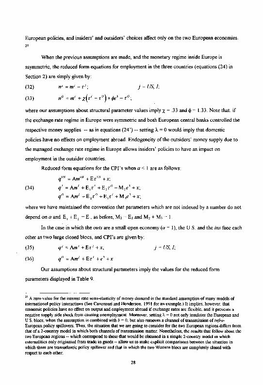
European policies, and insiders' and outsiders' choices affect only on the two European economies.
27
When the previous assumptions are made, and the monetary regime inside Europe is
asymmetric, the reduced form equations for employment in the three countries (equations (24) in
Section 2) are simply given by:
(32)
(33)
j ~US, I;
where our assumptions about structural parameter values imply X= .33 and«!>= 1.33. Note that, if
the exchange rate regime in Europe were symmetric and both European central banks controlled the
respective money supplies --as in equations (24') --setting A.= 0 would imply that domestic
policies have no effects on employment abroad. Endogeneity of the outsiders' money supply due to
the managed exchange rate regime in Europe allows insiders' policies to have an impact on
employment in the outsider countries.
(34)
Reduced form equations for the CPI's when a< I are as follows:
qus = Am"s +Erus +x;
qi =Ami +E 1ri +E,r 0- M,e' +x;
q 0 =Ami+ E 2 r 0 + E 1ri + M 3e3 + x;
where we have maintained the convention that parameters which are not indexed by a number do not
depend on a and E, + E, = E, as before, M2 = E2 and M2 + M, =I.
In the case in which the outs are a small open economy (a= 1), the U.S. and the ins face each
other as two large closed blocs, and CPI's are given by:
(35)
(36)
Our assumptions about structural parameters imply the values for the reduced form
parameters displayed in Table 9.
27 A zero value for the interest rate semi-elasticity of money demand is the standard assumption of many models of international policy interactions (See Canzoneri and Henderson. 1991 for an example.) It implies, however. that economic policies have no effect on output and employment abroad if exchange rates are flexible. and it prevents a negative supply side shock from causing unemployment. Moreover. setting A. ~ 0 not only insulates the European and U.S. blocs, when the assumption is combined with b ~ 0, but also removes a channel of transmission of infraEuropean policy spillovers. Thus, the situation that we are going to consider for the two European regions differs from that of a 2-country model in which both channels of transmission matter. Nonetheless, the results that follow about the two European regions -- which correspond to those that would be obtained in a simple 2-country model in which externalities only originated from trade in goods -- allow us to make explicit comparisons between the situation in which there are transatlantic policy spillover and that in which the two Western blocs are completely closed with respect to each other.
28
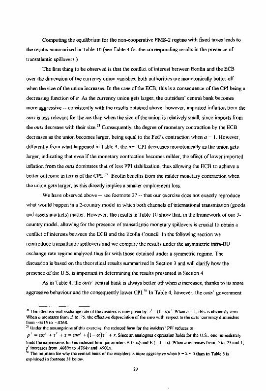
Computing the equilibrium for the non-cooperative EMS-2 regime with fixed taxes leads to
the results summarized in Table 10 (see Table 4 for the corresponding results in the presence of
transatlantic spillovers.)
The first thing to be observed is that the conflict of interest between Ecofin and the ECB
over the dimension of the currency union vanishes: both authorities are monotonically better off
when the size of the union increases. In the case of the ECB, this is a consequence of the CPI being a
decreasing function of a. As the currency union gets larger, the outsiders' central bank becomes
more aggressive -- consistently with the results obtained above; however, imported inflation from the
outs is less relevant for the ins than when the size of the union is relatively small, since imports from
the outs decrease with their size. 28 Consequently, the degree of monetary contraction by the ECB
decreases as the union becomes larger, being equal to the Fed's contraction when a= I. However,
differently from what happened in Table 4, the ins' CPI decreases monotonically as the union gets
larger, indicating that even if the monetary contraction becomes milder, the effect oflower imported
inflation from the outs dominates that ofless PPI stabilization, thus allowing the ECB to achieve a
better outcome in terms of the CPl. 29 Ecofin benefits from the milder monetary contraction when
the union gets larger, as this directly implies a smaller employment loss.
We have observed above -- see footnote 2 7 -- that our exercise does not exactly reproduce
what would happen in a 2-country model in which both channels of international transmission (goods
and assets markets) matter. However, the results in Table I 0 show that, in the framework of our 3-
country model, allowing for the presence of transatlantic monetary spillovers is crucial to obtain a
conflict of interests between the ECB and the Ecofin Council. In the following section we
reintroduce transatlantic spillovers and we compare the results under the asymmetric infra-EU
exchange rate regime analyzed thus far with those obtained under a symmetric regime. The
discussion is based on the theoretical results summarized in Section 3 and will clarifY how the
presence of the U.S. is important in determining the results presented in Section 4.
As in Table 4, the outs' central bank is always better off when a increases, thanks to its more
aggressive behaviour and the consequently lower CPl.'" In Table 4, however, the outs' government
"The effective real exchange rate of the insiders is now given by: z' = (I - a)z-'. When a= I, this is obviously zero. When a increases from .5 to . 75, the effective depreciation ofthe euro with respect to the outs' currency diminishes from -.0415 to -.0268. "Under the assumptions ofthis exercise. the reduced form for the insiders' PPI reduces to:
p 1 = an1 + 1J + x = am1 +(!-a )r 1 + x. Since an analogous expression holds for the U.S .. one immediately
finds the expressions for the reduced form parameters A(= o.) and E (= I - o.). When a increases from .5 to .75 and I, p1 increases from .4689x to .4764x and .490lx. '" The intuition for why the central bank of the outsiders is more aggressive when b = A. = 0 than in Table 5 is explained in footnote 31 below.
29
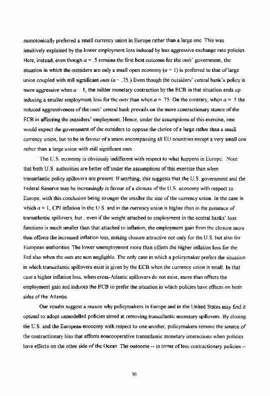
monotonically preferred a small currency union in Europe rather than a large one. This was
intuitively explained by the lower employment loss induced by less aggressive exchange rate policies
Here, instead, even though a= .5 remains the first best outcome for the outs' government, the
situation in which the outsiders are only a small open economy (a = I) is preferred to that oflarge
union coupled with still significant outs (a= .75.) Even though the outsiders' central bank's policy is
more aggressive when a = I, the milder monetary contraction by the ECB in that situation ends up
inducing a smaller employment loss for the outs than when a= . 75. On the contrary, when a = . 5 the
reduced aggressiveness of the outs' central bank prevails on the more contractionary stance of the
ECB in affecting the outsiders' employment. Hence, under the assumptions of this exercise, one
would expect the government of the outsiders to oppose the choice of a large rather than a small
currency union, but to be in favour of a union encompassing all EU countries except a very small one
rather than a large union with still significant outs
The U.S. economy is obviously indifferent with respect to what happens in Europe. Note
that both U.S. authorities are better off under the assumptions of this exercise than when
transatlantic policy spillovers are present. If anything, this suggests that the U.S. government and the
Federal Reserve may be increasingly in favour of a closure of the U.S. economy with respect to
Europe, with this conclusion being stronger the smaller the size of the currency union. In the case in
which a= I, CPI inflation in the U.S and in the currency union is higher than in the presence of
transatlantic spillovers, but, even if the weight attached to employment in the central banks' loss
functions is much smaller than that attached to inflation, the employment gain from the closure more
than offsets the increased inflation loss, making closure attractive not only for the U.S but also for
European authorities. The lower unemployment more than offsets the higher inflation loss for the
Fed also when the outs are non negligible. The only case in which a policymaker prefers the situation
in which transatlantic spillovers exist is given by the ECB when the currency union is small. In that
case a higher inflation loss, when cross-Atlantic spillovers do not exist, more than offsets the
employment gain and induces the ECB to prefer the situation in which policies have effects on both
sides of the Atlantic.
Our results suggest a reason why policymakers in Europe and in the United States may find it
optimal to adopt unmodelled policies aimed at removing transatlantic monetary spillovers. By closing
the U.S. and the European economy with respect to one another, policymakers remove the source of
the contractionary bias that affects noncooperative transatlantic monetary interactions when policies
have effects on the other side of the Ocean. The outcome -- in terms of less contractionary policies --
30
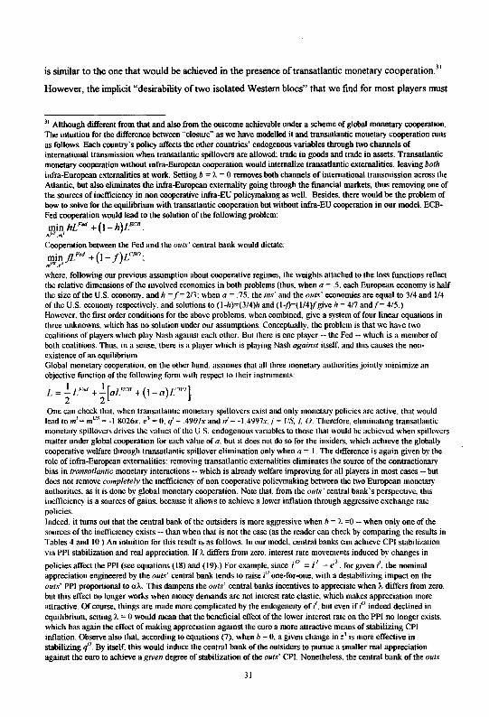
is similar to the one that would be achieved in the presence of transatlantic monetary cooperation.''
However, the implicit "desirability of two isolated Western blocs" that we find for most players must
31 Although different from that and also from the outcome achievable under a scheme of global monetaJy cooperation. The intuition for the difference between '"closure" as we have modelled it and transatlantic monetaJy cooperation runs as follows. Each countJy 's policy affects the other countries' endogenous variables through two channels of international transmission when transatlantic spillovers are allowed: trade in goods and trade in assets. Transatlantic monetaJy cooperation without infra-European cooperation would internalize transatlantic externalities, leaving both infra-European externalities at work. Setting b = A. = 0 removes both channels of international transmission across the Atlantic. but also eliminates the infra-European externality going through the financial markets. thus removing one of the sources of inefficiency in non cooperative infra-EU policymaking as well. Besides. there would be the problem of how to solve for the equilibrium with transatlantic cooperation but without infra-EU cooperation in our model. ECBFed cooperation would lead to the solution of the following problem:
min hLF«i +(1-h)LECH mus.ml
Cooperation between the Fed and the out'' central bank would dictate:
minj!_.''ed +(J- f)LCBO; mUT.l'J
where. following our previous assumption about cooperative regimes. the weights attached to the loss functions reflect the relative dimensions of the involved economies in both problems (thus, when a = .5. each European economy is half the size of the U.S. economy. and h =f= 2/3: when a= .75. the ins' and the outs' economies are eqnal to 3/4 and 1/4 of the U.S. economy respectively. and solutions to (l-h)=(3/4)h and (11)=(1/4lfgive h = 417 and.f= 4/5.) However. the first order conditions for the above problems. when combined. give a system offour linear equations in three unknowns. which has no solution under our assumptions. Conceptually. the problem is that we have two coalitions of players which play Nash against each other. But there is one player -- the Fed - which is a member of both coalitions. Thus. in a sense. there is a player which is playing Nash against itself. and this causes the nonexistence of an equilibrium. Global monetary cooperation. on the other hand. assumes that all three monetary authorities jointly minimize an objective function of the following form with respect to their instruments:
/_ = ~LF'J +~[aLECR +(1-a)L''HOl
One can check that. when transatlantic monetary spillovers exist and only monetaJy policies are active. that would lead to m1 = mus = -1.8026x, e3 = 0. q = .490/x and n' = -1.4997x, j ~ US, I, 0. Therefore. eliminating transatlantic monetaJy spillovers drives the values of the U.S. endogenous variables to those that would be achieved when spillovers matter under global cooperation for each value of a. but it does not do so for the insiders, which achieve the globally cooperative welfare through transatlantic spillover elimination only when a = I. The difference is again given by the role of infra-European externalities: removing transatlantic externalities eliminates the source of the contractionary bias in transatlantic monetary interactions -- which is already welfare improving for all players in most cases -- but does not remove completely the inefficiency of non cooperative policymaking between the two European monetary authorities. as it is done by global monetary cooperation. Note that. from the outs' central bank's perspective. this inefficiency is a sources of gains. because it allows to achieve a lower inflation through aggressive exchange rate policies. Indeed. it turns out that the central bank of the outsiders is more aggressive when b = A. =0 --when only one of the sources of the inefficiency exists -- than when that is not the case (as the reader can check by comparing the results in Tables 4 and 10.) An intuition for this result is as follows. In our model. central banks can achieve CPI stabilization via PPI stabilization and real appreciation. If A. differs from zero. interest rate movements induced by changes in
policies affect the PPI (see equations (18) and (19).) For example, since i 0 = i 1 - e3
• for given l. the nominal appreciation engineered by the outs' central hank tends to raise I'' one-for-one. with a destabilizing impact on the outs' PPI proportional to a.A.. This dampens the outs' central banks incentives to appreciate when A. differs from zero. but this effect no longer works when money demands are not interest rate elastic, which makes appreciation more attractive. Of course. things are made more complicated by the endogeneity of l. but even if i'' indeed declined in equilibrium, setting A. = 0 would mean that the beneficial effect of the lower interest rate on the PPI no longer exists, which has again the effect of making appreciation against the euro a more attractive means of stabilizing CPI inflation. Observe also that. according to equations (7). when b = 0, a given change in z3 is more effective in stabilizing q0
. BY itself, this would induce the central bank of the outsiders to pursue a smaller real appreciation against the euro to achieve a given degree of stabilization of the outs' CPl. Nonetheless, the central bank of the outs
31
not be overstated. On the one hand, it may be easier for the involved authorities to improve their
welfare by explicitly coordinating their policies rather than by working to close the respective
economies. On the other hand, our model is an extremely simplified description of reality: even
though under the assumptions of this section policies aimed at closing the two blocs with respect to
one another would be mutually beneficial in most cases, in a more realistic setting, in which, for
example, trade policy is explicitly considered, policies to close the U.S. and European blocs may well
have welfare decreasing effects also due to the retaliations that aggressive trade policies are likely to
cause32 Besides, even without considering trade policy, it may be possible that, if fiscal
policymakers are active players in the game, conflicts of interests among the players over the benefits
from "closure" of the two Western blocs or transatlantic monetary cooperation become relevant33 34
7 A symmetric exchange rate regime in Europe
We now reintroduce transatlantic policy spillovers and compare the results obtained so far, under the
assumption of an asymmetric monetary regime in Europe, with the case of flexible exchange rates:
both the ECB and the central bank of the outsiders control the respective money supplies and e3 is
determined endogenously and left free to float. As mentioned in the introduction such a regime is the
relevant alternative to the policymakers' plan to set up a new EMS linking insiders and outsiders. 35
When the infra-European monetary regime is symmetric, the reduced forms of the model are
given by equations (23') through (26'.) The computations for the non cooperative monetary game
when fiscal policies are fixed are summarized in Table II. When we compare the results in this table
with those reported in Table 4, for the corresponding case of an asymmetric monetary regime, we
immediately see that once again -- like when we had assumed away all transatlantic policy spillovers
has a zero CPI target -- which is different from achieving the same CPI as in Table 4 -- and this consideration, coupled with the arguments sketched above about the impact on= 0, helps understanding the central bank's increased aggressiveness when transatlantic spillovers are removed. 32 Basevi, Delbono. and Denicolo' (1990) analyze a formal model of monetary and trade interactions. For some contributions to the debate on trade and currency areas, see Federal Reserve Bank of Kansas City (1991.) 33 See Ghironi and Eichengreen ( 19%) for a discussion of disagreements between central banks and governments on the desirability of transatlantic monetary cooperation. 34 As the results of Table 10 are sufficient to make the point that "the pre5ence of the U.S. does make a difference" in our model, we do not discuss here the results of the simulated game when infra-EU monetary cooperation and fiscal activism are considered. It is possible to show that, when monetary cooperation is coupled with (limited) fiscal activism, all players agree on the desirability of a small currency union under the assumptions of this section. The results of the simulations are available from the authors upon request. 35 The debate maiuly focuses on an EMS-style arrangement versus a flexible exchange rate regime coupled with inflation targeting. Here, in order to focus on the role of the exchange rate regime in affecting the results, rather than assuming rigid inflation targeting rules, we maintain the assumption that central banks choose their instruments to minimize loss functions in which a much larger weight is attached to inflation than to unemployment. The implications of rigid inflation targeting are discussed by Persson and Tabellini (1996.) Frankel ( 1989) analyzes alternative rules for the conduct of monetary policy.
32
-- the conflict of interests between the ECB and the Ecofin Council disappears. Both authorities
monotonically prefer a large union to a small one. Ecofin's preference for the large union is
intuitively justified by the behaviour of employment as a varies. Instead, the ECB turns out to be
better off when inflation is relatively high than when it is lowest (a= .5.)
In order to interpret the results for the alternative infra-EU regimes and to understand the
role of the U.S. in our model, it is important to refer to the results summarized in Section 3 about the
tradeoffs faced by the various policymakers. We know from the discussion in that section that, under
the symmetric infra-EU exchange rate regime, when the outs' size is non negligible (a< 1), the
insiders face a more favourable tradeoff than the United States. Nonetheless, the ECB ends up being
worse off than the Fed, and this happens not withstanding the fact that c/ is smaller than qus The
crucial point is that the ECB, which has to cope with the impact of the outs' central bank aggressive
policy when a< I, "rides" its more favourable tradeoff with respect to the Fed's one much more
aggressively, the more so the smaller is a, in a successful attempt at exporting inflation to the U.S.
via real appreciation of the euro against the dollar. However, in doing so, the ECB imposes an
employment loss to the ins' economy which more than offsets the inflation gain, even if the weight
attached to employment in the central banks' loss functions is much smaller than that attached to
inflation. As we move from the small currency union towards the situation in which the outs are
negligible, the ins' tradeoff approaches the United States', and the incentive for the ECB to "ride"
aggressively a more favourable tradeoff with respect to the Fed's is removed. Even if c/ rises, the
ECB is made better off by the relevant employment gain.
When the infra-EU exchange rate regime was asymmetric and significant outs existed (Table
4), the ECB preferred a small union because, facing the same tradeoff as the U.S. irrespective of the
union's size, the ins' central bank had a smaller incentive to dump the outs' aggressive behaviour to
the U.S. economy. As a consequence of this, the ECB's monetary stance was always less
contractionary than in Table 11 and, as we have seen, when the union was large, the milder monetary
contraction ended up destabilizing the PPI. With a symmetric exchange rate regime in Europe, the
ECB prefers the large union for exactly the opposite reason: facing a more favourable tradeoff than
the U.S., the ins' monetary authority has a much stronger incentive to "ride" it aggressively in order
to export to the U.S. the inflation it imports from the outs-- the more so the smaller the currency
union -- but this has destabilizing consequences on employment which outweigh the inflation gain. 36
36 This argument is consistent with the pattern of the dollar-euro real exchange rate that we observe in our simulations: the dollar appreciates in real terms against the euro under the EMS-2 regime, but it depreciates under the symmetric regime, when the ECB implements a much more aggressive monetary policy vis-a-vis the Fed. Besides. the results of this exercise seem to suggest that the potential gains from "approximating transatlantic cooperation via
33
Note that, as it should have been expected, the infra-European exchange rate regime is irrelevant
when a= I -- in that case the results in Table II and in Table 4 are identical. When the outsiders are
negligible, the monetary arrangement governing infra-EU interactions is irrelevant also from the
outs' perspective because in that case the tradeoffs faced by all authorities do not change across
exchange rate regimes in Europe.
If the outs' are non negligible and the infra-EU regime is symmetric, their central bank prefers
a large rather than a small union -- as it happened in Table 4 -- because in that situation it achieves a
better stabilization of the CPI, which offsets the employment loss due to a more contractionary
stance. The central bank of the outsiders is more aggressive when a= .75 than when a= I, even
though its tradeoff is better in the latter case. Still, the outs' central bank achieves a better outcome
in terms of the CPI when a= I, and suffers a smaller employment loss than when the outs are non
negligible. This is an example of a situation in which, faced with a more favourable tradeoff, the
policymaker refrains from "riding it" very aggressively, optimally trading control of inflation for
employment stabilization. When the infra-EU exchange rate regime is symmetric and their size is
negligible, the outs can thus achieve the same outcome as under the EMS-2 regime without having
to increase the contractionary character of their policy with respect to the case a= .75. The intuition
for this result lies in the different characteristics of the alternative exchange rate regimes in Europe.
As the reader can check by comparing the reduced form equations under the two regimes, when the
managed exchange rate regime is implemented in Europe, due to the endogeneity constraint on m0,
the reduction in the ins' monetary contraction going from a = . 75 to a= I has a harmful impact on
the outs' CPl. As a consequence, the outs' central bank optimally reacts by strengthening its
contractionary stance. When the endogeneity constraint on m0 is removed and the infra-European
monetary arrangement is symmetric, going from a= . 75 to a = I, the less contractionary policy by
the ECB is beneficial in terms of stabilizing q0 -- and rrl has a larger impact on it. Consequently, the
central bank of the outsiders reacts optimally by loosening its stance. Note that when a = . 75, the
outs' CPI is lower under the symmetric regime than under the asymmetric one, but this reduction in
the CPI is achieved at the cost of a relevant employment loss, which ends up making the outs' central
bank worse off under the symmetric regime.
The previous observations make it clear why the government of the outsiders considers being
a "small open economy" the first best situation under a symmetric regime, but would choose the
small union outcome rather than the large union. In Tables 4 and I 0, a= .5 was the best possible
isolation of the two Western blocs", could be bigger when both European central banks control the respective money supplies. as this induces more contractionary transatlantic interactions than those in Table 4.
34
outcome for the outs' government, as explained above. As we go through our exercises, a = 1 raises
from the bottom to the top position in the ranking of the outs' government's preferences37 The
change between the EMS-2 regime with and without transatlantic externalities has been motivated in
Section 5, whereas the difference between the asymmetric and the symmetric regimes with
transatlantic spillovers is intuitively explained by the outs' central bank behaviour. With a= .5 there
is no way for the central bank of the outsiders to actually export inflation to the ins, given the
completely symmetric positions of the two European central banks. Thus, although the
contractionary bias of non cooperative policies still exists, the monetary stance of the outs' central
bank is less contractionary than when a= . 75, when the central bank can actually take advantage of a
more favourable tradeoff than the ins' and does it aggressively. When a rises from . 75 to 1, the
outsiders' employment-inflation tradeoff improves further, as it happened under the asymmetric
regime, but the central bank manages to achieve the same outcome as under that regime by means of
a less contractionary policy than when a= .75 and only slightly more contractionary than when a=
.5. Combined with the ECB's and the Fed's less contractionary policies-- motivated by the fact that
their tradeoffs are now equal -- this contributes to give the best employment outcome for the outs'
economy when a = I, contrary to what happened under the asymmetric regime.
Finally some remarks on the U.S. authorities. Differently from the ECB, the Fed's ranking of
preferences when the infra-EU regime is symmetric is driven by the inflation outcome. The U.S.
central bank considers a = 1 the best possible situation, but would prefer a large union rather than a
small one when the outs' are a significant entity. Hence, when a< I, there is a preference reversal
with respect to what happened when the EMS-2 regime was implemented in Europe. Again, the
results summarized in Section 3 help us understand what happens. Under the EMS-2 regime, both
the ECB and the Fed always face identical tradeoffs, and both suffer from the outs' aggressive
behaviour when a= . 75. When the infra-EU regime is asymmetric, the ECB does not have the
possibility of exploiting a more favourable tradeoff when the ins' size is smaller than the United
States'. Instead, ifthe exchange rate regime in Europe is symmetric and the outs are non negligible,
the ECB faces a more favourable tradeoff than the Fed, the more so the smaller the currency union.
As we have noted above, a consequence of this is that the ECB's attitude towards the U.S. monetary
authority in dumping on it the consequences of non cooperative policies within Europe is much more
aggressive when a= .5 than when a= . 75. Besides, as it happened under the EMS-2 regime, the
outs' central bank always faces a better tradeoff than the Fed, and it faces the same tradeoff as the
" Letting >- denote "preferred to" and omitting the a's, nnder the EMS-2 regime, the ranking of the outs' government preferences was: .5 >- .75 >- l; onder "closure" of the two Western blocs, it was: .5 >- l >- .75; and under the symmetric regime we have l >- .5 >- .75.
35
ECB's when a= .5. Even though the tradeoff faced by the outs' worsens as a changes from .75 to
.5, when the infra-EU exchange rate regime is symmetric, the overall monetary stance ofEurope
towards the U.S.-- measured by [ani+ (l-a)m0] --is more aggressive when the currency union is
small. When a= .75, the ECB's policy is less contractionary, while the outs' central bank is more
aggressive. Combining these observations with the fact that, as the reader can check, the effect of m1
on q118 is larger when a = . 7 5 and the impact of m0 is larger when a = . 5 explains why the U.S.
central bank suffers a bigger loss in the latter situation38
Thanks to the change in the Fed's ranking of preferences, both the monetary authority and
the U.S. government share the same ranking of preferences when the infra-European monetary
arrangement is symmetric-- and no cross-regime preference-reversal happens for the U.S.
government. The monetary contraction implemented by the Fed is tougher the smaller the currency
union, reacting to the policies implemented by the two European central banks. As a consequence,
even though the Fed does not achieve the goal of having lowest inflation when the union is smallest,
the employment loss increases as the size of the currency union decreases, and the U.S. government
monotonically prefers a large union outcome rather than the small union case.
What would happen if the two European central banks cooperated with one another in the
game in which only monetary policies are used actively? The answer is straightforward, as we know
from Section 4. Results for the U.S. and insiders' authorities would coincide with those obtained in
the absence of cooperation with a = 1, while the outs' variables and losses would be "driven" to the
same values as for the U.S. and the ins' ones in the a = 1- no cooperation case. No exchange rate
change would be observed. Consequently, policymakers in the U.S. and in the insider countries
would favour monetary cooperation inside Europe, analogously to what happened under the
asymmetric exchange rate regime of Section 4. Instead, a conflict of interests would arise between
the outsiders' government and central bank. The former would like European central banks to
cooperate, as this would greatly reduce its unemployment loss. But the latter would be prevented
from using the exchange rate as a strategic device to stabilize inflation, and would suffer from a
larger loss.
Tables 12 and 13 describe the outcome when (limited) fiscal activism is introduced, in the
case of a symmetric monetary regime with and without cooperation, respectively. 39
38 We remark that the key in driving the result is the change in the position of the ins' employment-inflation tradeoff with respect to the U.S. one, the outs' tradeoff being unchanged across infra-EU regimes. 39 We recall that in the case oflimited fiscal activism governments choose taxes to minimize:
L'"' = H·z[.t(q'Y +9(n')']+.8( •')'}; 1 =us. 1. o.
36
As in Section 5, adding active fiscal policies as stabilizing devices against the impact of the
shock has a welfare improving effect for all players. In the case of monetary cooperation, since the
infra-EU exchange rate regime is symmetric, if a= .5, even if fiscal externalities are not internalized,
the euro-outs exchange rate does not move because optimal policies are identical for both the ins'
and the outs' policymakers. The exchange rate between insiders and outsiders does move when a=
.75, in which case optimal policies differ. Insiders' authorities prefer a small rather than a large union
and the same is true for U.S. policymakers. Instead, the outsiders' central bank and government both
prefer a large rather than a small union. These results are analogous to those presented in Table 6 for
the case of an asymmetric regime in Europe. We leave it to the reader to interpret them on the basis
of the intuitions and tools provided throughout the paper.
All policymakers are better off when governments can use fiscal policy to react to exogenous
shocks, even in the absence of monetary cooperation. In this case we observe again a conflict of
interests between Ecofin and the ECB on the desired size of the European currency union: the ECB
prefers a small union, while Ecofin prefers a large one. This is different from what happened under
the EMS-2 regime in Europe (Table 7), in which case both the insiders' authorities preferred the
small union outcome. The difference in the ranking ofEcofin's preferences with respect to Table 7 is
due to the fact that, under the symmetric regime, the employment loss increases as the size of the
union decreases, while the opposite happened under the EMS-2 regime. When a= .5 and the
exchange rate regime is symmetric, the European authorities face identical employment-inflation
tradeoffs. As the size of the outs increases from a= 1 to a= .5, the tradeoff faced by the ECB
becomes steeper. The symmetry between ins and outs that is achieved when a= .5 induces the ECB
to behave more aggressively, differently from what happened in the EMS-2 case of Table 7, with
contractionary consequences on the ins' economy. The small union case represents the first best for
the outs' government, whereas the central bank monotonically prefers a large union. Both U.S.
policymakers favour the small union case over the large one. Again, we leave it to the reader to go
deeper into the interpretation of the results presented above40
8 Conclusions
In this paper we have addressed the issue of the optimal size of the European currency union
concentrating our attention on the effects of the interactions among fiscal and monetary authorities in
Europe, and between Europe and the rest of the world. We have argued that explicitly considering
40 A thorough discussion of the results obtained when fiscal authorities are active players in the game would require references to the tradeoff's faced by the governments under the symmetric infra-EU regime. We refrain from exploring the issue here for reasons of brevity.
37
the presence of the rest of the world-- that we have called "the U.S."-- is important in
understanding policymak.ers' incentives and behaviour. In our analysis, we have always maintained
the same assumptions about the way European and U.S. authorities interact with each other, i.e. non
cooperatively and under a flexible exchange rate regime.41
Consider the institutional setup that, we believe, will most likely characterize the future
working of EMU: frozen fiscal policies and non cooperative monetary policies under an EMS-2
regime in Europe. In this setup, the view that central bankers would prefer the currency union to be
relatively small, while Ecofin would prefer it to be relatively larger, is confirmed by our analysis -
provided the size of the outsiders is non negligible. The only way to obtain an agreement between
Ecofin and the ECB on the desired size of the currency union is either by convincing the central
banks of the ins and outs to cooperate (in which case the size of the currency union becomes
irrelevant), or by allowing governments to actively use fiscal policy in response to exogenous shocks.
But the outsider central bank stands to loose from cooperating with the ECB --independently of the
degree of fiscal policy activism and of the size of the outsiders relative to the insiders. Moreover, it
always prefers the currency union to be relatively large because this is the situation in which it can
best exploit its ability to export inflation to the insiders by aggressively "riding" the more favourable
output-inflation tradeoff it faces. This suggests a potentially important reason (which may run against
different arguments in favour of joining the single currency) why some states may be unwilling to
join the currency union and, once they are out, their central banks may be unwilling to enter a
cooperative agreement with the ECB.
Table 14 shows the preference rankings of the various players over the size of the European
currency union for the case of non cooperative monetary interactions with fixed taxes in the three
different environments that we have analyzed: EMS-2, closed Western blocs, and flexible exchange
rates in Europe. In the table, the a's are omitted to save on notation, and >- denotes "preferred to",
whereas "" denotes "indifferent to".
For almost all players and in all the three different settings that we have analyzed, the
situation in which the currency union in Europe encompasses the whole EU except for a small entity
is the first best outcome. This result parallels that obtained by Alesina and Grilli (1994), though in a
different model and under different assumptions. The one authority which does not always prefer
that outcome is the outs' government, which ranks a= I first only when the exchange rate regime in
Europe is symmetric for the reasons discussed above.
41 Alternative transatlantic arrangements are studied in Ghironi (1993) and Ghironi and Eichengreen (1996.) In both those analyses, EMU is assumed to encompass the whole EU, so that there are no outs. Those models, however, allow for the absence of fiscal cooperation within the currency union.
38
Potential conflicts of interests can arise within one country over the optimal size of the
currency union. Not only we find a conflict between Ecofin and the ECB under the EMS-2 regime in
Europe, but also, while the central bank of the outsiders always prefers a= .75 to a= .5, the
opposite holds for the outs' government. Given a significant size for the outs, the latter would always
choose a small rather than a large currency union. Also the Federal Reserve and the U.S. government
may disagree over the optimal size of the European currency union if an EMS style regime were to
be implemented in Europe, with the Fed preferring a small union and the U.S. a large one if a< I.
Nonetheless, even if U.S. policymakers will be interested spectators of what happens in Europe and
transatlantic interactions do affect all policymakers' welfare, it does not seem likely that European
policymakers will condition their choices about the size of the currency union in 1998 and in the
following years on U.S. authorities' preferences.
As our model suggests, in 1998, when the initial size of the currency union is to be decided,
strategic interactions among players could justify considerable strain in the choice process. This may
be true irrespective of monetary and fiscal policymakers having different preferences across
countries. The outcome will depend on the relative bargaining power of the various involved
policymakers as well as on other political considerations that our model does not capture. The
institutional framework within which the policymakers interact will play a crucial role in this process.
Note that the outs' government always prefers a small rather than a large union, when a is
not 1, and that a currency union leaving only a negligible entity outside is not likely in 1998. This
observation suggests that, if we explicitly allow for a multiplicity of outsiders' governments, rather
than a single government which has "preferences over the size of its country", all of them could want
to stay out of the union when this comes to life, because the small union outcome is more attractive
to them. As a consequence, it would be hard to find outs' governments actually willing to join the
union either from its beginning or after that time. Resistance by outsiders' governments to join could
lead to an initially relatively small currency union, thus meeting the preferences of the ECB if the
EMS-2 regime were to be implemented. The intuition about a multiplicity of outs' governments
cannot be overstated, however. The conclusion of our model is based on the assumption that the
outs act as a unified bloc, which is analogous to assuming that all outs' central banks cooperate with
each other and all outs' governments do the same. Allowing for the possibility of non cooperative
strategic interactions within the group of the outsiders may significantly affect the results, and would
allow a better analysis of the problem.42 We leave this issue for further research on the topic.
42 Recall that we have also implicitly assumed that all ins' governments cooperate within the Ecofin Council, but this need not be the case.
39
The previous observations lead us naturally to a second set of remarks. After the Initial size
of the currency union has been chosen, the natural evolution of the union itself as dictated by the
Maastricht Treaty would be its enlargement over time to cover the whole European Union. Our
result that a= 1 is the first best outcome for most players-- including the U.S.! --lends support to
the advocates of the desirability of such outcome. Suppose that potential conflicts between the ECB
and the Ecofin Council either are not an issue or are resolved in favour of the enlargement option43
Still, the results of our simulations suggest that the remaining outs' governments may not find joining
the union attractive.
The analysis of our paper assumes that all players approach 1998 and the subsequent period
starting from equal initial conditions, their economies being in equilibrium, and addresses the topic
from the limited perspective of the optimal reactions to a supply side disturbance. Reality is much
more complicated, though. In 1998 European countries will be likely to be characterized by different
economic situations. Outs may be outs either because they are not attracted by the perspective of
joining the union or because they are not accepted in it or for both reasons. It is plausible that most
outsiders economies will be classified as relatively weak or plagued by significant disequilibria. If
their governments do not have strong incentives to join the European currency union -- and our
model suggests potential reasons why this could happen-- the process of enlargement of the union
envisioned in the Maastricht Treaty could prove itself slower and more conflictive than optimists
normally argue.
One of the interpretations of how the process of European integration in different fields has
evolved over time has to do with the idea of positive spillovers from the economic to the social and
political arena, with integration starting in the economic field, deepening and then being extended to
the other areas. The facts of the past lend support to this idea. But if the preferences of the outs'
governments were to become an obstacle, this could break down the whole process when the biggest
obstacle of the past-- German resistance and fear-- seems to be overcome. Fortunately, strong
objections can be raised against this argument. The obvious one is that the simple analysis of this
paper overlooks important political economy arguments that would explain why the outsiders are
indeed likely to eventually join the union.44 The process of integration in Europe is indeed driven
43 At least in the first few years after the beginning of Stage III. it is likely that also the European Council will indeed attach a great value to monetary stability and to the establishment of the reputation of the ECB. Nonetheless. it is not unrealistic to think about conflictive situations of the type that we are analyzing being resolved in favour of the Ecofin Council. Our model is not suited to analyze if this could have negative consequences on the ECB's reputation. even if a simple intuition suggests that this may not be the case, as the ECB would be forced to accept the Council's decisions. 44 See Eichengreen and Ghironi ( 1996) for a discussion of these arguments.
40
mainly by political reasons, which have their roots in historical events. A failure in the process of
Western European integration before, or at least together with, enlargement to the Eastern European
countries, would probably lead to Germany -- and not the EU -- deepening its integration with the
latter countries, facilitated by historical linkages and economic interdependencies. As a consequence
of the potential economic strength of this bloc, Mediterranean countries, but also the UK, would
bear the risk of living" ... in a Continent that, in any case, will dance to the tune of Germany, but
where other countries will find their views much more difficult to be heard." Our model cannot
capture these aspects of the whole process, but it suggests reasons other than cross-country
differences in preferences why different policymakers may have different incentives in approaching
EMU. Combining these economic incentives with political considerations in a unified framework
would allow to give a comprehensive analysis of the problem, but this is well beyond the aims of this
paper and it is also left for future work.
Finally, there is another dimension of the choices that the various policymakers will face by
1998 which deserves attention in this conclusion: for given initial size of the currency union, what is
going to be the optimal infra-European monetary arrangement? Our analysis has been mainly focused
on the choice of the optimal size of the European currency union, but the results that we have
obtained with our simulations allow to give tentative answers to this other crucial question. In order
to give an example, we focus our attention on the case of fixed fiscal policies and no cooperation,
which seems to be the most likely one. Table 15 summarizes the players' preference rankings in the
choice between a non-cooperative EMS-2 regime (denoted by A) and the non-cooperative flexible
exchange rate regime (denoted by B.) The rankings are based on the results reported in Table 4 and
in Table II.
When the European currency union includes all countries except for a small open economy,
all players are indifferent as for the exchange rate regime that prevails in Europe, which is intuitively
justified by the absence of any impact of the outs' policy choices on the rest of the world. But when
the outsiders are non-negligible, in most cases the EMS-2 regime turns out to be preferred to the
flexible exchange rate regime. This is justified by the results that we have discussed in the previous
sections. Controlling the exchange rate allows the outsiders' central bank to achieve a better
outcome than what would be achieved by controlling the money supply. Under the asymmetric
regime, the employment loss is smaller, and the outs' government is consequently better off.
Therefore, at least if fixed fiscal policies and no cooperation represent a likely scenario, the results of
our exercise suggest that the outs' authorities will favour the adoption of an EMS style regime over
that of a flexible rate arrangement. Instead, we observe a conflict of interests between the ECB and
41
Ecofin over what regime should be implemented. As it could have been expected on the basis of the
results and intuitions discussed above, the ECB would like a flexible exchange rate regime to be
adopted since this would allow it to achieve a significantly better inflation outcome by depriving the
outs' central bank of control over the exchange rate. Nonetheless, this would come at the cost of
higher employment losses, which induce Ecofin to prefer the managed exchange rate regime.
This further conflictive dimension of the debate among different policymakers over the
optimal features of the European currency union does not seem to be completely unlikely. Reasons
of brevity prevent us from presenting analogous tables for the other policymaking regimes we have
considered. The interested reader can easily reconstruct them from the material presented above and
interpret the results using the tools and intuitions discussed in the paper. Nonetheless, tables 14 and
15 are enough to drive home an important point ofthis paper: as 1998 approaches, conflicts of
interests between policymakers are likely to arise on the different issues they face. We have discussed
above the problems that may be caused by disagreements over the optimal size of the union. But
also, analyses of alternative monetary arrangements between the ins and the outs in the post-EMU
era should take the possibility of conflicts of interests among policymakers within one group or the
other as well as across countries into account. This would increase the realism of the discussions and
could improve the reliability of any normative suggestion based on them. Some ways to deal with the
conflicts to which we have referred -- and with the many others that we have probably overlooked -
will have to be found to ensure a proper functioning to the European integration process. The way
institutions are designed and political developments will play a crucial role with respect to these
problems.
One more observation is in order before closing this paper. In all our simulations we have
seen that some degree of fiscal activism makes all authorities better off with respect to the situation
in which only monetary policy is used to react against the consequences of the supply side shock.
This result may be interpreted as an argument against the rigid application of a "fiscal stability pact"
in Europe. However, the way fiscal policy is modelled in our paper is extremely simplified. Indeed, if
fiscal stability is interpreted as referring to the behaviour of deficits and debts, active budget
balancing fiscal policies as those considered in the paper are not inconsistent with a "fiscal stability
pact" and some flexibility of fiscal policy would be welfare improving, as the results of our
simulations suggest. In order to provide a more thorough analysis of the role of fiscal policy as an
active instrument available to policymakers and of the issue of fiscal discipline, extending the model
to a multiperiod framework in which deficits and debt accumulation are allowed would be necessary.
This is another line along which we believe it is worth extending our research in the future.
42
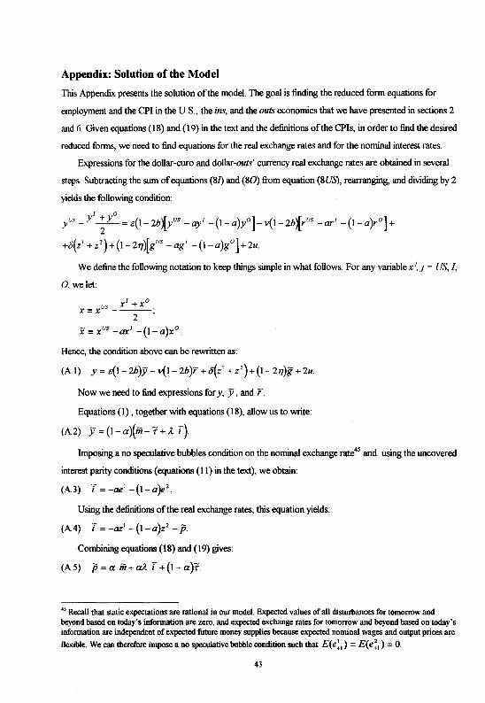
Appendix: Solution of the Model
This Appendix presents the solution of the model. The goal is finding the reduced form equations for
employment and the CPI in the U.S., the ins, and the outs economies that we have presented in sections 2
and 6. Given equations (18) and (19) in the text and the definitions of the CPis, in order to find the desired
reduced forms, we need to find equations for the real exchange rates and for the nominal interest rates.
Expressions for the dollar -euro and dollar -outs' currency real exchange rates are obtained in several
steps. Subtracting the sum of equations (81) and (80) from equation (SUS), rearranging, and dividing by 2
yields the following condition:
Y I +yo y 118
---
2-=c(1-2b)[yus -a;/ -(1-a)y0]-v(1-2h~rus -ar1 -(1-a)r 0 ]+
+o(z' +z')+(1-2q~gus -ag1 -(1-a)g 0 ]+2u.
We define the following notation to keep things simple in what follows. For any variable x1, j = US, I,
0, we let:
Hence, the condition above can be rewritten as:
Now we need to find expressions for y, y, and r.
Equations (I), together with equations (18), allow us to write:
(A2) Ji=(l-a)(m-i'+A. i).
Imposing a no speculative bubbles condition on the nominal exchange rate45 and using the uncovered
interest parity conditions (equations (II) in the text), we obtain:
(A.3) i=-ae 1 -(1-a)e 2.
Using the definitions of the real exchange rates, this equation yields:
(A4) T = -az1 - (1- a)z2
- p.
Combining equations (18) and (19) gives:
(AS) p=am+aA.i+(1-a)i'.
45 Recall that static expectations are rational in our model. Expected values of all disturbances for tomorrow and beyond based on today' s information are zero, and expected exchange rates for tomorrow and beyond based on today· s information are independent of expected future money supplies because expected nominal wages and output prices are
flexible. We can therefore impose a no speculative bubble condition such that £(<,) = E(e;,) = 0.
43
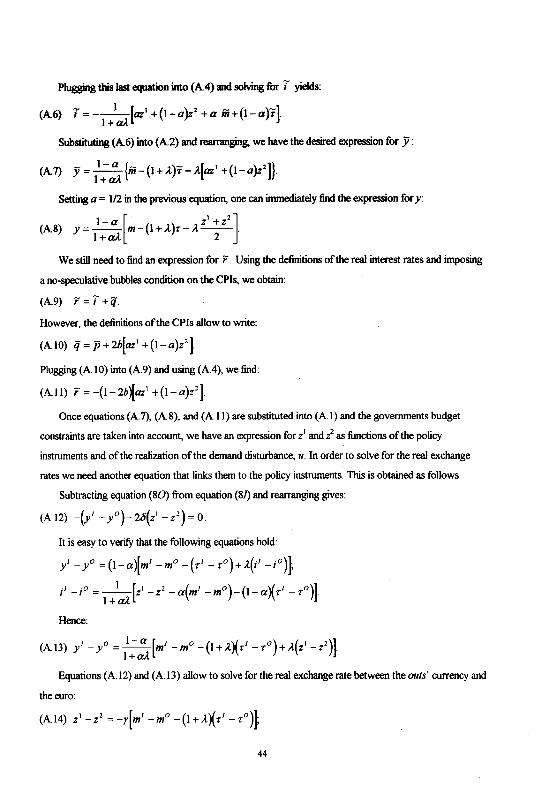
Plugging this last equation into (A4) and solving for i yields:
(A6) '{ = --1-(az1 +(1-a}z2 +a m+(1-a)rl
1+aA. J"
Substituting (A6) into (A.2) and rearranging, we have the desired expression for y:
(A7) y= /:~ {m-(1+.-t)'i'-..t[az• +(1-a)z2)}.
Setting a= 112 in the previous equation, one can immediately find the expression for y:
1-a[ z1
+z2
] (A.8) y=-- m-(1+.-t)r-..t--. 1+aA. 2
We still need to find an expression for r. Using the definitions of the real interest rates and imposing
a no-speculative bubbles condition on the CPis, we obtain:
(A.9) r = i +if.
However, the definitions of the CPis allow to write:
(A.lO) 'ij= p+2b[az1 +(1-a)z2].
Plugging (A.lO) into (A.9) and using (A4), we find:
(All) r = -(1-2hXaz• +(l-a)z2].
Once equations (A. 7), (A.8), and (All) are substituted into (AI) and the governments budget
constraints are taken into account, we have an expression for z1 and :l- as functions of the policy
instruments and of the realization of the demand disturbance, u. In order to solve for the real exchange
rates we need another equation that links them to the policy instruments. This is obtained as follows.
Subtracting equation (80) from equation (81) and rearranging gives:
(A.I2) -v -y 0)- 2o(z1
- z2) = 0.
It is easy to verity that the following equations hold:
/ - y 0 = (1-a)[m1- m0
- (•1
- r 0 )+..t(i 1 -i 0n ;I -io = l+laA.[z•-z2 -a(mi -mo)-(t-aXTJ _,a)].
Hence:
(A.l3) YJ _yo= /:~[mi -mo -(l+..t)(•J _,a)+..t(z• -z2}].
Equations (A.12) and (A13) allow to solve for the real exchange rate between the outs' currency and
the euro:
(A.I4) z 1 -z2 =-r[m1 -m0 -(l+..tXr1 --r0 )~
44
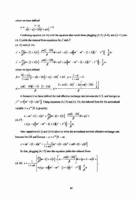
where we have defined:
1-a r= A.(1-a)+28(1+aA.)>O.
Combining equation (A 14) with the equation that results from plugging (A 7), (AS), and (A 11) into
(A I) yields the reduced form equations for z1 and:?:
(A15)and(A16)
, p ( ( ) ] pe(l- 2b) _ - ( )[ 1 0 ( ')( 1 0 )] 2 z =p m- 1+..1. r- f3 m+rpr-y 1-J.t m -m - 1+~~. r -r -fju;
z' = ~(m-(1+..t)rJ-pe(1; 2b) m+rpr+rf.l[m1 -m0 -(l+..tXr1 -r0 )J-%u; where we have defined:
f3=..t(l-a)(1-e(1-2b)]+v(1-2b) 2 +28; p= 1-a >0; l+a.-1. l+aA
ep(1_ 2b)(l+A.)-(1_ 277) 8+av(l-2b)' -..t;{w(1-2b)-k]
rp= f3 ;J.l= f3
In footnote 6 we have defined the real effective exchange rate between the U.S. and Europe as
z118 = b[az' + (1- a)z']. Using equations (A 15) and (A 16), the reduced form for the normalized
variable z = z118 /b is given by:
Also, equations (A3) and (A6) allow to write the normalized nominal effective exchange rate
between the US and Europe-- e = e118 /b --as:
e=ae 1 +(1-a)e' =-1-[az' +(1-a)z' +am+(l-a)T].
1+aA
So that, plugging (A 17) into this equation yields the reduced form:
lf.[m-(1 + ..t)r] +[a- pe(l- 2b) 1;;:; +(rp + 1- a)r +)
(A18) e=-1 - f3 f3 J" .
1 + aA ( \f 1 0 ( \{ 1 0)] 2 +r J.t-a'lm -m - 1+..1.1\r - r -fju
45
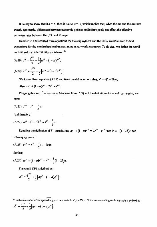
It is easy to show that if a= .5, then it is alsop= .5, which implies that, when the ins and the outs are
exactly symmetric, differences between economic policies inside Europe do not affect the effective
exchange rates between the U.S. and Europe.
In order to find reduced form equations for the employment and the CPis, we now need to find
expressions for the nominal and real interest rates in our world economy. To do that, we define the world
nominal and real interest rates as follows: 46
.w ;us I [ ·I ·O] (A.19) 1 =z-+"2 a1 +(1-a~ ;
w ,.us I [ I 0] (A.20) r =--z+"2 ar +(i-a}r .
We know from equation (A. II) and from the definition of z that: r = -(I - 2b )z.
Plugging this into T = -e- which follows from (A.3) and the definition of e --and rearranging, we
have:
And therefore:
(A.22) ai 1 +(1- a)i 0 = ;w +.!.e. 2
Recalling the definition of r ' substituting ar I + (I - a )r 0 = 2r w - r us into r = -(I - 2h )z and
rearranging gives:
(A.23) ,.us = r"' - _!_(1- 2h )z. 2
So that:
I (A.24) ar1 +(1-a)r 0 =rw +-(1-2h)z.
2
The world CPI is defined as:
w qus I [ I o] q =--z+"2 aq +(1-a)q ;
46 In the remainder of the appendix, given any variable :1, j = l!.S, /, 0, the corresponding world variable is defined as w xus I I 0
x = 2 +2[ax +(1-a)x ].
46
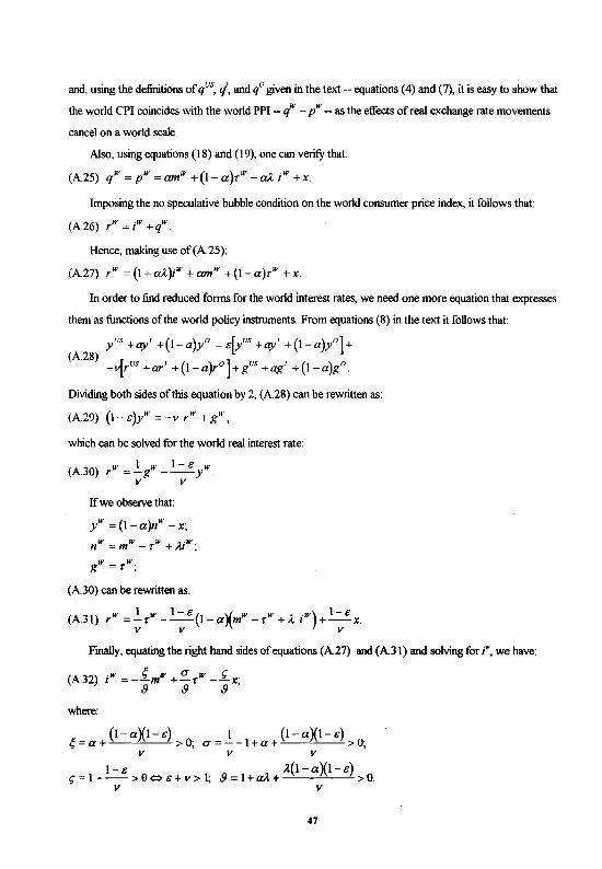
and, using the definitions of qus, q, and q0 given in the text -- equations ( 4) and (7), it is easy to show that
the world CPI coincides with the world PPI -- q"' ~ pw -- as the effects of real exchange rate movements
cancel on a world scale.
Also, using equations (18) and ( 19), one can verity that:
(A.2S) qw = pw = amw +(1- a)rw + aA. iw +x.
Imposing the no speculative bubble condition on the world consumer price index, it follows that:
(A.26) rw = iw +qw
Hence, making use of(A.25):
(A.27) rw = (1 + aA.}iw + amw +{I- a)rw +X.
In order to find reduced forms for the world interest rates, we need one more equation that expresses
them as functions of the world policy instruments. From equations (8) in the text it follows that:
(A.28) y'JS +£9'1 +(I-a)yo = s[yus +£9'1 +(1-a)yo]+
-v[rus +ar1 +(1- a)ro] +gus +ag1 + (!- a)go
Dividing both sides of this equation by 2, (A.28) can be rewritten as:
(A.29) (1- s)yw = -v rw + g",
which can be solved for the world real interest rate:
(A 30) w _ I w I - s w
. r --g ---y . v v
If we observe that:
yw =(1-a)nw -x;
nw = mw _ Tw + ,uw;
gw = Tw;
(A.30) can be rewritten as:
w I w 1- s ( )( w w •W) 1- s (A.31) r =-r --- I-a m -T +A. 1 +--x. v v v
Finally, equating the right hand sides of equations (A.27) and (A.31) and solving for r, we have:
(A.32) i"' =-.£mw +~r"' _.f.x· f) f) f)'
where:
(1- a)(!- s) ,;=a+ >0;
1 (1- a)(1- s) cr=--I+a+ >0;
v v v I-s il(1-a)(1-s)
~ = 1 - -- > 9 (:) s + v > 1; f) = 1 + aA. + > 0. v v
47
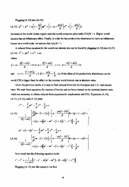
Plugging (A32) into (A25):
(A.33) qw = pw = a(1- i)mw +(1-a+ ~a}.w +(1- i)x. Increases in the world money supply raise the world consumer price index if'Af/S < 1. Higher world
taxation has an inflationary effect. Finally, in order for the productivity disturbance to have an inflationary
impact on a world scale, we assume that a.MjS < I.
A reduced form equation for the world real interest rate can be found by plugging (A.32) into (A27):
(A.34) rw = q,w + lTw + ~;
where:
""=a- ;{1+aA.) >O~a> ~(l+aA.). 1=1-a+ a(1+aA.) >0· ., 8 8 ' 8 '
and o = 1- (l + aA.)~ > 0 if 1- aA.~ >.f., i.e. if the effect of the productivity disturbance on the 8 8 8
world CPI is bigger than the effect on the nominal world interest rate in absolute value.
Given the previous results, it is easy to find reduced forms for the European and U.S. real interest
rates. We omit those equations for reasons ofbrevity and we focus instead on the nominal interest rates,
which are necessary to obtain reduced form equations for employment and CPis. Equations (A.l8),
(A.21), (A.22), and (A.32) yield:
.us ~ w a w ~ 1 = --m +-r --x+
8 8 8
(A.35) _ 1 ~~[m-(l+A.)rJ+[a-pe(l; 2b)]m+(qJ+l-a}T+I· 2(1 + aA.) ( "If I 0 ( X I 0)] 2 ' +r ,u-a'lm -m - l+A. r - r -pu
·I (I ).a ~ w a w ~ a1 + -a 1 = --m +-T --x+ 8 8 8
(A.36) 1 ~~[m-(l+A.)rJ+[a-pe(l; 2b)]m+(tp+l-a)r+l + 2(1 + aA) ( )[ I 0 ( )( I 0)] 2 . +r ,u-a m -m - I+A. r -r -pu
Now recall that the foUowing equation holds:
;I -io = l+laA.[z' -z' -a(mi -mo)-(1-aX•I _,o)].
Plugging (A.14) into this equation we find:
48
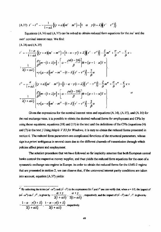
(A37) i 1 -i0 =-I+IaA. {(r+a)(m1 -m0 )+[1-a-y(I+A.)Kr1 -r-
0)}.
Equations (A36) and (A37) can be solved to obtain reduced fonn equations for the ins' and the
outs' nominal interest rates. We find:
(A38) and (A.39)
. 1 I - a {( )( 1 o) [ ( ')K 1 o )} .; w a w t; I =-I+aA y+a m -m + I-a-y 1+/L T -T --am +-aT --ax+
+ I ~~[m- (1 + A.)r] + [a- pe(1;
2b) ]iii+ (rp +I- a)T +]-
2(I+aA.) ( \1" 1 o ( )( 1 o)] 2 , +r ,u-a-'l.m -m - l+A. r -r -pu
47
Given the expressions for the nominal interest rates and equations (A 14), (A 15), and (A 16) for
the real exchange rates, it is possible to obtain the desired reduced forms for employment and CPis by
using those equations, equations (IS) and (19) in the text and the definitions of the CPis (equations (4)
and (7) in the text.) Using Maple V R3 for Windnws, it is easy to obtain the reduced forms presented in
section 6. The reduced fonn parameters are complicated functions of the structural parameters, whose
sign is a priori ambiguous in several cases due to the different channels of transmission through which
policies affect prices and employment.
The solution procedure that we have followed so far implicitly assumes that both European central
banks control the respective money supplies, and thus yields the reduced fonn equations for the .case of a
symmetric exchange rate regime in Europe. In order to obtain the reduced fonns for the EMS-2 regime
that are presented in section 2, we can observe that, if the uncovered interest parity conditions are taken
into account, equation (A37) yields:
47 By coUecting the tenns (,/- m") and ( -1- -f) in the expressions for I and ,.o one can verilY that, when a = 112, the impact of
(I o,. 1 .o . . by a+r a+r ............... _ .. , andthe. f(-1 .P. J .v. . by
11r-m 1 on ,1 ,tsgwen ( ) , ( ) , • ....,........~J, unpacto -• 1 on1 ,1 .tsgwen 2 1+aA. 2 l+aA.
1-a-y(l+A.) 1-a-y(l+A.} . 2(l+aA..), 2(l+aA..) ,respectively.
--49
(A.40)i1 -i0 = -1
+1aA. {(r+aXm1 -m0 )+(1-a-y(l+l)Kr1 -r0 )}=e' -e2 =e'.
This equation can be solved for m0 as a function of e3, rrl, .f, and I, thus yielding the endogeneity
constraint that is imposed on the outs' money supply under the EMS-2 regime:
(A.41) m0 =m1 +z(r1 -r0 )+¢e';
where we have defined the parameters x and ell to simplii'y the notation. The reader can easily check from
the definition of y and by working out the expressions for J( and ell that these parameters do not depend on
the size of the European currency union, a. By plugging equation (A. 41) into the reduced forms obtained
following the procedure described above, one obtains the reduced form equations for the EMS-2 regime
presented in section 2.
References
Alesina, A. and V. Grilli (1994), "On the Feasibility of a One-Speed or Multispeed Monetary Union", in B. Eichengreen and J. Frieden (eds.), The Political Economy of European MonetlU)' Unification. Westview Press, 107-128.
Alesina, A. and G. Tabellini ( 1987), "Rules and Discretion with Noncoordinated Monetary and Fiscal Policies", Economic Enquiry 25, 619-630.
Basevi, G., F. Delbono e V. Denicolo' (1990), "International Monetary Cooperation under Tariff Threats", Journal of International Economics 28.
Bruno, M., and J. Sachs (1985), Economics ofWorldwide Stagflation. Harvard University Press.
Buiter, W., G. Corsetti and P. Pesenti (1996), "A Centre-Periphery Model ofMonetary Coordination and Exchange Rate Crises", CEPR Discussion Paper no. 1201.
Canzoneri, M. B. and D.W. Henderson (1991), Monetary Policy in Interdependent Economies: A Game-Theoretic Approach. Cambridge: MIT Press.
De Grauwe, P. (1996), "The Pros and Cons of a Mini Currency Union", unpublished, University of Leuven.
Eichengreen, B., and F. Ghironi (1996), "European Monetary Unification: The Challenges Ahead," in Francisco Torres (ed.), MonetlU)' Reform in Europe, Lisbon: Universidade Catolica Editora, pp. 83-120 (also CEPR Discussion Paper No. 1217).
Europe Documents (1992): Treaty on European Union, Maastricht.
Federal Reserve Bank of Kansas City (1991), Policy Implications of Trade and Currency Zones, Proceedings of a Symposium Sponsored by the Federal Reserve Bank of Kansas City, Jackson Hole, Wyoming.
50
Frankel, J. A. (1989), "International Nominal Targeting (INT): A Proposal for Overcoming Obstacles to Policy Coordination," in J. McCallum and R. Mundell (eds.), Global Disequilibrium.
Ghironi, F. ( 1993 ), "Regimi di tasso di cambio e coordinamento internazionale delle politiche economiche: Che cosa abbiamo imparato in dieci anni di letteratura?". Tesi di Laurea, unpublished, Universita' L. Bocconi.
Ghironi, F. and B. Eichengreen (1996), "U.S.-Europe Policy Interactions: From the Post-Bretton Woods era to EMU'', unpublished, University of California, Berkeley.
Ghironi, F. and F. Giavazzi (1997), "Size Matters: Currency Unions and the Employment-Inflation Tradeoff", unpublished, IGIER, Universita Bocconi, Milano.
Giavazzi, F. and A. Giovannini ( 1989), "Monetary Policy Interactions under Managed Exchange Rates", Economica 56, 199-213.
Giavazzi, F. and M. Pagano (1996), "Non-Keynesian Effects ofFiscal Policy Changes: International Evidence and the Swedish Experience", Swedish Economic Policy Review, vol. 3, no.1, Spring, pp. 67-103.
Kenen, P. B. (1995), Economic and Monetary Union in Europe: Moving Beyond Maastricht. Cambridge: Cambridge University Press.
Persson, T., and G. Tabellini (1996), "Monetary Cohabitation in Europe", CEPR Discussion Paper no. 1380.
Rogoff, K. (1985), "Can International Monetary Cooperation Be Counterproductive?", Journal of International Economics 18,199-217.
Spaventa, L. (1996), "Out in the Cold? Outsiders and Insiders in 1999: Feasible and Infeasible Options", CEPR Discussion Paper no. \379.
von Hagen, J. and M. Fratianni (1991), "Policy Coordination in the EMS with Stochastic Asymmetries", in Wihlborg, C., M. Fratianni and T.D. Willet (eds.), Financial Regulation and Monetary Arrangements after 1992. Amsterdam: Elsevier Science Publishers.
Wyplosz, C. (1996), "An EMS for Both "ins" and "outs': the Contractual and Conditional Approach", Swiss Political Science Review, 2, (Spring) pp. 178-83.
S!
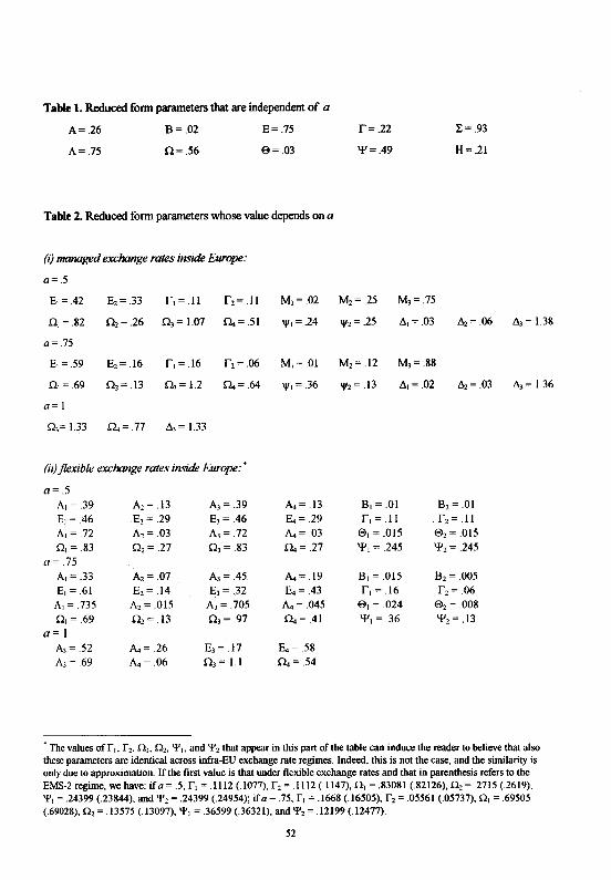
Table 1. Reduced form parameters that are independent of a
A=.26 B=.02 E=.75
A=.75 0=.56 e=.03
Table 2. Reduced form parameters whose value depends on a
(i) managed exchange rates inside Europe:
a= .5
E1 =.42 E, = .33 r,=.ll r, = .11
n,=.s2 n,= .26 n,= 1.01 n.= 51
a= .15
E, =.59 E,= .16 r, =.16 r, = .06
n,=.69 n,= .13 n,= 1.2 n.= .64
a= I
n,= 1.33 n.= .77 Ll, = 1.33
(ii) flexible exchange rates inside Europe:'
a=.5 A1 = .39 A2 = .13 A3 =.39 E, = .46 E2 = .29 E3 =.46 II.,= .72 A2 = .03 A3 = .72 n, = .83 n,= .27 n,= .83
a= .15 A,= .33 A2 = .07 A3 =.45 E1 =.61 E2 = .14 E3 = .. 32
II.,= .735 A 2 = .015 A3 = .705 n, = .69 n,= .13 n,=.97
a= I A3 =.52 ~=.26 E3 = .17 11.,=.69 A.= .06 n, = 1.1
M1 =.02
"'' = .24
M1 =.01
"'' = .36
~=.13
E4 = .29 A.= .03 n.= .27
~=.19
E4 = .43 A.= .045 n.= .41
E.= .58 n.= .54
r=.22
'I'= .49
I=.93
H=.21
M2 = .25 M3 =.75
'l'z= .25 Ll,=.03 Ll, = .06
M2 =.12 M3 = .88
"'' = .13 Ll, = .02 Ll, = .03
B, =.01 B2 = .01 r,=.II r, =.II
e, =.015 e,= .015 '1', = .245 '1', = .245
B1 = .015 B2 = .005 r, = .16 r, = .06
e, = .024 e,= .oos '1', = .36 '1', = .13
Ll, = 1.38
Ll, = 1.36
·The values ofr,. r 2• n" n,, '1'1, and '1'2 that appear in this part of the table can induce the reader to believe that also these parameters are identical across infra-EU exchange rate regimes. Indeed. this is not the case, and the similarity is only due to approximation. If the first value is that under flexible exchange rates and that in parenthesis refers to the EMS-2 regime, we have: if a= .5, r, = .1112 (.1077), r, = .1112 (.1147), n, = .83081 (.82126), 0 2 = .2715 (.2619), '1'1 = .24399 (.23844), and '¥2 = .24399 (.24954); if a= .75, r, = .1668 (.16505), r, = .05561 (.05737), n, = .69505 (.69028), n, = .13575 (.13097), '1'1 = .36599 (.36321), and '¥2 = .12199 (.12477).
52
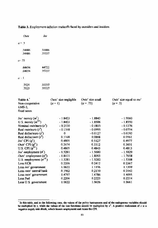
Table 3. Employment-inflation tradeoffs faced by outsiders and insiders
Outs Ins
a= .5
.54486
.54486
a=.75
.64654
.64654
a= I
.54486
.35337
.44722
.35337
. 7525 .35337
.7525 .35337
Table 4." Non-cooperative EMS-2, fixed taxes.
Ins' money (nf) U.S. money (mu8
)
Nominal outs/euro (e3)
Real outs/euro (i) Real dollar/euro (z1
)
Real dollar/outs (z2)
Ins' CPI (c/) Outs' CPI (q0
)
U.S. CPI (qu8)
Ins' employment (rl) Outs' employment (n~ U.S. employment (nus) LossECB Loss ins' government Loss outs' central bank Loss outs' government Loss Fed Loss U.S. government
Outs' size negligible Outs' size small (a= I) (a= .75)
- 1.8423 - 1.8843 - 1.8423 - 1.8506 - 0.2130 - 0.1815 -0.1168 -0.0995
0 -0.0127 0.1168 0.0868 0.4805 0.5127 0.2674 0.3312 0.4805 0.4843
- 1.5281 - 1.5680 -1.8111 - 1.8093 - 1.5281 - 1.5282
0.2206 0.2412 1.0622 1.1196 0.1962 0.2130 1.4797 1.4786 0.2206 0.2223 1.0622 1.0626
Outs' size equal to ins' (a= .5)
- 1.9060 - 1.8550 -0.1376 -0.0754 -0.0193
0.0561 0.4977 0.3601 0.4813
- 1.5829 - 1.7658 - 1.5308
0.2367 1.1399 0.2142 1.4095 0.2214 1.0661
• In this table, and in the following ones, the values of the policy instruments and of the endogenous variables should be multiplied by x, while the values of the loss functions should be multiplied by ~- A positive realization of x is a negative supply side shock, which lowers employment and raises the CPl.
53
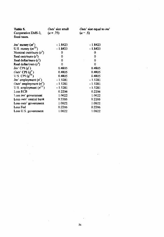
Table 5. Outs' size small Outs' size equal to ins' Cooperative EMS-2, (a= .75) (a= .5) fixed taxes.
Ins' money (,/) - 1.8423 - 1.8423 U.S. money (mu8
) - 1.8423 - 1.8423 Nominal outsleuro (e3
) 0 0 Real outs/euro (?) 0 0 Real dollar/euro (z1
) 0 0 Real dollar/outs (z2
) 0 0 Ins' CPI (q') 0.4805 0.4805 Outs' CPI (q0
) 0.4805 0.4805 U.S. CPI (qu8
) 0.4805 0.4805 Ins' employment (d) - 1.5281 - 1.5281 Outs' employment (n°) - 1.5281 - 1.5281 U.S. employment (nus) - 1.5281 - 1.5281 LossECB 0.2206 0.2206 Loss ins' government 1.0622 1.0622 Loss outs' central bank 0.2206 0.2206 Loss outs' government 1.0622 1.0622 Loss Fed 0.2206 0.2206 Loss U.S. government 1.0622 1.0622
54
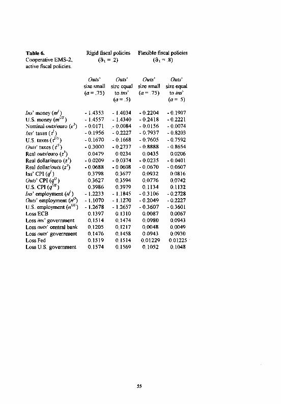
Table 6. Rigid fiscal policies Flexible fiscal policies Cooperative EMS-2, Uh = .2) (~h = .8) active fiscal policies.
Outs' Outs' Outs' Outs' size small size equal size small size equal (a= .75) to ins' (a= .75) to ins'
(a= .5) (a= 5)
Ins' money (m') - 1.4353 - 1.4034 -0.2204 -0.1907 US. money (mus) - 1.4557 - 1.4340 -0.2418 - 0.2221 Nominal outs/ euro ( e3
) -0.0171 -0.0084 - 0.0156 -0.0074 Ins' taxes (!) -0.1956 -0.2227 - 0.7937 -0.8203 U.S taxes ( fls) -0.1670 - 0.1668 - 0.7605 - 07592 Outs' taxes (.f) -0.3000 - 0.2737 -0.8888 -0.8654 Real outsleuro (i) 0.0479 0.0234 0.0435 0.0206 Real dollar/euro (z1
) -0.0209 -0.0374 -0.0235 - 0.0401 Real dollar/outs (z2
) -0.0688 -0.0608 -0.0670 -0.0607 Ins' CPI (q') 0.3798 0.3677 0.0932 0.0816 Outs' CPI ( q0
) 0.3627 0.3594 0.0776 0.0742 U.S CPI (qus) 0.3986 0.3979 0.1134 0.1132 Ins' employment (tt) - 1.2233 - 1.1845 -0.3106 -0.2728 Outs' employment (n~ - 1.1070 - 1.1270 -0.2049 -0.2227 U.S. employment (nus) - 1.2678 - 1.2657 -0.3607 -0.3601 Loss ECB 0.1397 0.1310 0.0087 0.0067 Loss ins' government 0.1514 0.1474 0.0980 0.0943 Loss outs' central bank 0.1205 0.1217 0.0048 0.0049 Loss outs' government 0.1476 0.1458 0.0943 0.0930 Loss Fed 0.1519 0.1514 0.01229 0.01225 Loss U.S. government 0.1574 0.1569 0.1052 0.1048
55
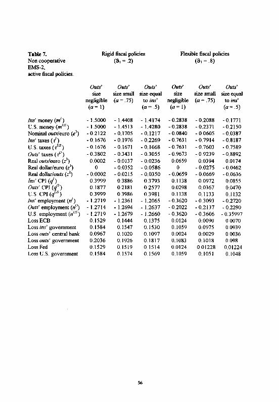
Table 7. Rigid fiscal policies Flexible fiscal policies Non cooperative (SI = .2) (S1 = .8) EMS-2, active fiscal policies.
Outs' Outs' Outs' Outs' Outs' Outs' size size small size equal size size small size equal
negligible (a= .75) to ins' negligible (a= .75) to ins' (a= I) (a= .5) (a= 1) (a= .5)
Ins' money (ni) - 1.5000 - 1.4408 - 1.4174 -0.2838 -0.2088 -0.1771 U.S. money (mu8
) - 1.5000 - 1.4513 - 1.4280 - 0.2838 - 0.2371 -0.2150 Nominal outs/euro (e3
) -0.2122 -0.1705 -0.1217 -0.0840 -0.0605 -0.0387 Ins' taxes ( i) -0.1676 -0.1976 -0.2269 -0.7631 -0.7914 - 0.8187 US. taxes (fi8
) -0.1676 -0.1671 -0.1668 - 0.7631 -0.7603 - 0.7589 Outs' taxes (-f) -0.3802 - 0.3431 - 0.3055 - 0.9673 -0.9239 - 0.8892 Real outs/euro (z3
) 0.0002 -0.0137 -0.0236 0.0659 0.0394 0.0174 Real dollar/euro (z1) 0 -0.0352 -0.0586 0 -0.0275 -0.0462 Real dollar/outs(?) -0.0002 -0.0215 - 0.0350 -0.0659 -0.0669 -0.0636 Ins' CPI ( t/) 0.3999 0.3886 0.3793 0.1138 0.0972 0.0855 Outs' CPI (q0
) 0.1877 0.2181 0.2577 0.0298 0.0367 0.0470 U.S CPI (qus) 0.3999 0.3986 0.3981 0.1138 0.1133 01132 Ins' employment (n1
) - 1.2719 - 1.2361 - 1.2065 -0.3620 -0.3093 -0.2720 Outs' employment (n°) - 1.2714 - 1.2694 - 1.2637 -0.2022 - 0.2137 -0.2290 U.S employment (nus) - 1.2719 - 1.2679 - 1.2660 -0.3620 -0.3606 - 0.35997 LossECB 0.1529 0.1444 0.1375 0.0124 0.0090 0.0070 Loss ins' government 0.1584 0.1547 0.1530 0.1059 0.0975 0.0939 Loss outs' central bank 0.0967 0.1020 0.1097 0.0024 0.0029 0.0036 Loss outs' government 0.2036 0.1926 0.1817 0.1083 0.1018 0.098 Loss Fed 0.1529 0.1519 0.1514 0.0124 0.01228 0.01224 Loss US. government 0.1584 0.1574 0.1569 0.1059 0.1051 0.1048
56
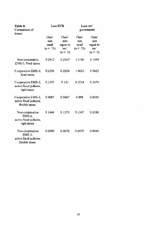
Table 8. LossECB Loss ins' Comparison of government losses.
Outs' Outs' Outs' Outs' size size size size small equal to small equal to
(a= .75) ins' (a= .75) ins' (a= .5) (a= 5)
Non-cooperative 0.2412 0.2367 1.1196 l.l399 EMS-2, fixed taxes.
Cooperative EMS-2, 0.2206 0.2206 1.0622 1.0622 fixed taxes.
Cooperative EMS-2, 0.1397 0.131 0.1514 0.1474 active fiscal policies,
rigid taxes.
Cooperative EMS-2, 0.0087 0.0067 0.098 0.0943 active fiscal policies,
flexible taxes.
Non-cooperative 0.1444 0.1375 0.1547 0.1530 EMS-2,
active fiscal policies, rigid taxes.
Non-cooperative 0.0090 0.0070 0.0975 0.0939 EMS-2,
active fiscal policies, flexible taxes.
57
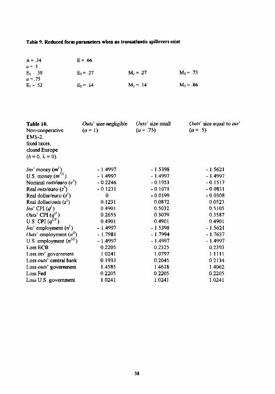
Table 9. Reduced form parameters when no transatlantic spillovers exist
A= .34 E= .66 a= .5 E1 = .39 E2 = .27 M2= .27 M3 = .73 a= .75 E, =.52 E2= .14 M2= .14 M3 = .86
Table 10. Outs' size negligible Outs' size small Outs' size equal to ins' Non-cooperative (a= I) (a= .75) (a= .5) EMS-2, fixed taxes, closed Europe (b = 0, A.= 0).
Ins' money(,/) - 1.4997 - 1.5398 - 1.5621 U.S. money (mus) - 1.4997 - 1.4997 - 1.4997 Nominal outsleuro (e3
) -0.2246 - 0.1953 -0.1517 Real outsleuro (i) -0.1231 -0.1071 - 0.0831 Real dollar/euro (z1
) 0 - 0.0199 -0.0308 Real dollar/outs (z2
) 0.1231 0.0872 0.0523 Ins' CPI (q) 0.4901 0.5032 0.5105 Outs' CPI ( q0
) 0.2655 0.3079 0.3587 US. CPI (qus) 0.4901 0.4901 0.4901 Ins' employment (d) - 1.4997 - 1.5398 - 1.5621 Outs' employment (rP) - 1.7981 - 1.7994 - I. 7637 U.S. employment (nus) - 1.4997 - 1.4997 - 1.4997 LossECB 0.2205 0.2325 0.2393 Loss ins' government 1.0241 1.0797 I. Ill! Loss outs' central bank 0.1933 0.2045 0.2134 Loss outs' government 1.4585 1.4618 1.4062 Loss Fed 0.2205 0.2205 0.2205 Loss U.S. government 1.0241 1.0241 1.0241
58
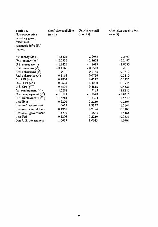
Table 11. Outs' size negligible Outs' size small Outs' size equal to ins' Non-cooperative (a= I) (a= .75) (a= .5) monetary game, fixed taxes, symmetric infra-EU regime.
Ins' money (ni) - 1.8423 -2.0955 -2.2497 Outs' money (m0
) - 2.2532 -2.3023 - 2.2497 U.S. money (mus) - 1.8423 - 1.8619 - 1.8685 Real outs/euro (i) -0.1168 -0.0588 0 Real dollar/euro (z1
) 0 -0.0138 0.3810 Real dollar/outs (z2
) 0.1168 0.0726 0.3810 Ins' CPI ( q') 0.4804 0.4272 0.3735 Outs' CPI ( q0
) 0.2674 0.3200 0.3735 US. CPI (qus) 0.4804 0.4818 0.4823 Ins' employment (1t) - 1.5281 - 1.7195 - 1.8315 Outs' employment (n°) -1.8111 - 1.8620 - 1.8315 U.S employment (nus) - 1.5281 - 1.5324 - 1.5339 Loss ECB 0.2206 0.2230 0.2305 Loss ins' government 1.0623 1.3397 1.5164 Loss outs' central bank 0.1962 0.2194 0.2305 Loss outs' government 1.4797 1.5653 1.5164 Loss Fed 0.2206 0.2219 0.2223 Loss U.S. government 1.0623 1.0683 1.0704
59
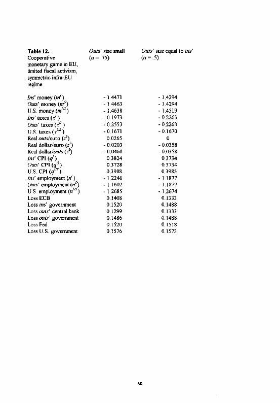
Table 12. Outs' size small Outs' size equal to ins' Cooperative (a= .75) (a= .5) monetary game in EU, limited fiscal activism, symmetric infra-EU regime.
Ins' money (rrl) - 1.4471 - 1.4294 Outs' money (m'1 - 1.4463 - 1.4294 U.S. money (m118
) - 1.4638 - 1.4519 Ins' taxes (I ) -0.1973 -0.2263 Outs' taxes ( -f ) - 0.2553 -0.2263 U.S. taxes ( fl8
) -0.1671 -0.1670 Real outs/euro (i) 0.0265 0 Real dollar/euro (z1
) - 0.0203 - 0.0358 Real dollar/outs(~) -0.0468 - 0.0358 Ins' CPI ( q') 0.3824 0.3734 Outs' CPI (q0
) 0.3728 0.3734 U.S. CPI (q118
) 0.3988 0.3985 Ins' employment (n1
) - 1.2246 - l.l877 Outs' employment (n'1 - 1.1602 - l.l877 U.S. employment (n118
) - 1.2685 - 1.2674 LossECB 0.1408 0.1333 Loss ins' government 0.1520 0.1488 Loss outs' central bank 0.1299 0.1333 Loss outs' government 0.1486 0.1488 Loss Fed 0.1520 0.1518 Loss U.S. government 0.1576 0.1573
60
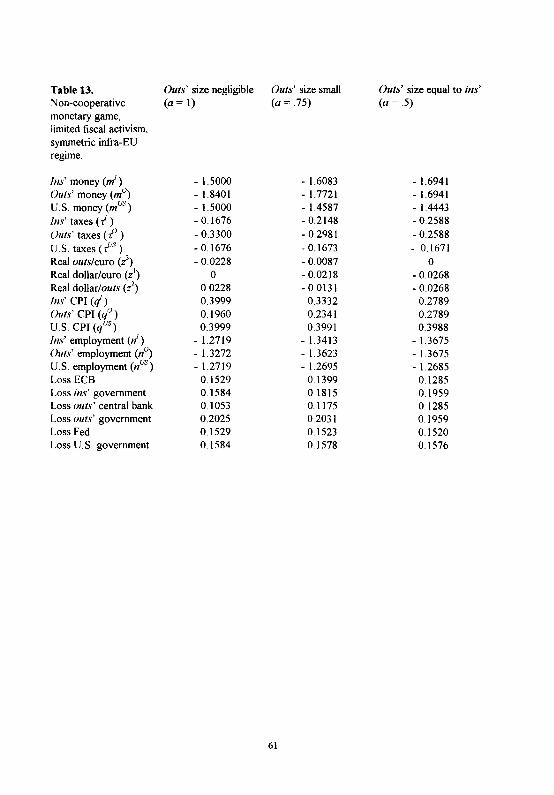
Table 13. Outs' size negligible Outs' size small Outs' size equal to ins' Non-cooperative (a= 1) (a= .75) (a= .5) monetary game, iimited fiscal activism. symmetric infra-EU regime.
Ins' money (m1) - 1.5000 - 1.6083 - 1.6941
Outs' money (m0) - 1.8401 - 1.7721 - 1.6941
U.S money (mus) - 1.5000 - 1.4587 - 1.4443 Ins' taxes ( t ) - 0.1676 -0.2148 - 0.2588 Outs' taxes (I' ) - 0.3300 - 0.2981 - 0.2588 U.S. taxes ( ps) - 0.1676 -0.1673 - 0.1671 Real outs/euro (i) -0.0228 -0.0087 0 Real dollar/euro (z1
) 0 -0.0218 -0.0268 Real dollar/outs (i) 0.0228 - 0.0131 - 0.0268 Ins' CPI ( q) 0.3999 0.3332 0.2789 Outs' CPI ( q0
) 0.1960 0.2341 0.2789 U.S. CPI (qus) 0.3999 0.3991 0.3988 Ins' employment (n1
) - 1.2719 - 1.3413 - 1.3675 Outs' employment (n°) - 1.3272 - 1.3623 - 1.3675 US. employment (nus) - 1.2719 - 1.2695 - 1.2685 Loss ECB 0.1529 0.1399 0.1285 Loss ins' government 0.1584 0.1815 0.1959 Loss outf' central bank 0.1053 0.1175 0.1285 Loss outs' government 0.2025 0.2031 0.1959 Loss Fed 0.1529 0.1523 0.1520 Loss U.S. government 0.1584 0.1578 0.1576
61
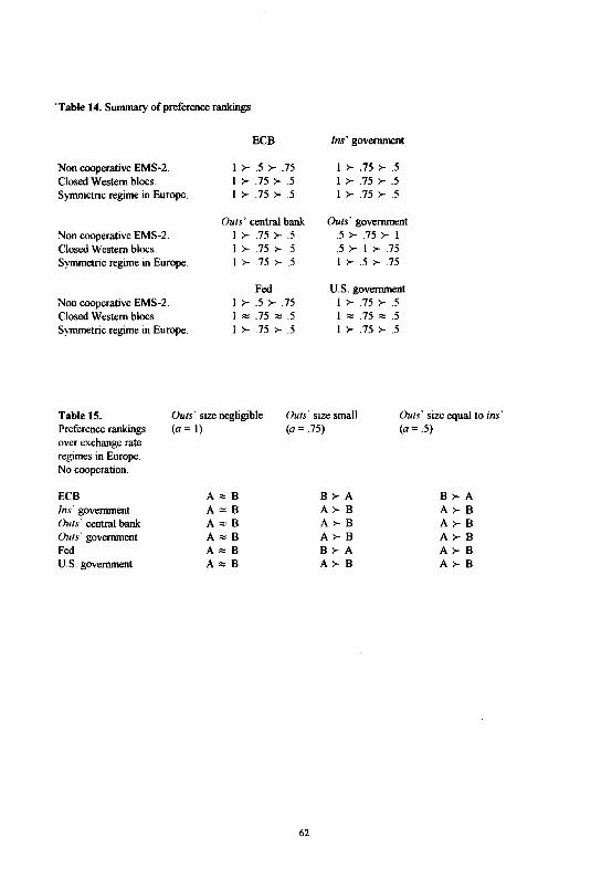
'Table 14. Sununary of preference rankings
Non cooperative EMS-2. Closed Western blocs. Symmetric regime in Europe.
Non cooperative EMS-2. Closed Western blocs. Symmetric regime in Europe.
Non cooperative EMS-2. Closed Western blocs. S~mmetric regime in Europe.
ECB
I >- .5 >- .75 I >- .75 >- .5 I >- .15 >- .5
Outs' central bank I >- .15 >- .5 I >- .15 >- .5 I >- .75 >- .5
Fed I >- .5 >- .75 I ,., .15 ,., .5 I >- .15 >- .5
Ins' government
I >- .75 >- .5 I >- .75 >- .5 I >- .75 >- .5
Outs 0 government .5 >- .15 >- I .5 >- I >- .75 I >- .5 >- .75
U.S. government I >- .75 >- .5 I ,., .75 ,., .5 I >- .75 >- .5
Table 15. Outs 0 size negligible Outs 0 size small Outs 0 size equal to ins'
Preference rankings (a= I) (a= .75) (a= .5) over exchange rate regimes in Europe. No cooperation.
ECB A::::B B>-A B>-A Ins
0 government A,.,B A>-B A>-B Outs
0 central bank A::::B A>-B A>-B Outs
0
government A::::B A>-B A>-B Fed A::::B B>-A A>-B U.S. government A::::B A>-B A>-B
62
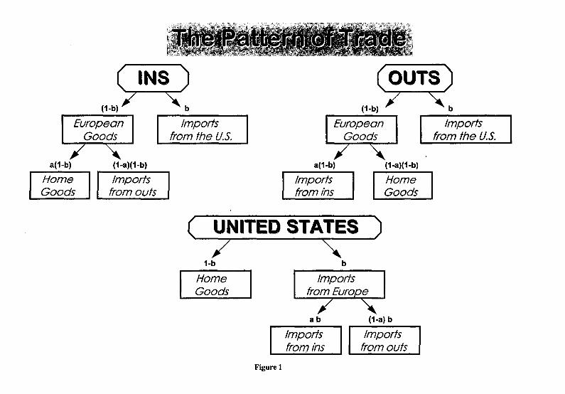
(1~~ 11~~UT~ .--------, r-------.
a(1-b)
Home Goods
(1-a)(1-b)
Imports from outs
Imports from the U.S.
a(1-b)
Imports from ins
(1-a)(1-b)
Home Goods
( UNITED STATES ) 7 ~
1-b
I Home I Goods
Figure 1
ab
Imports from ins
b
(1-a) b
Imports from outs
.------...., Imports
from the U.S.
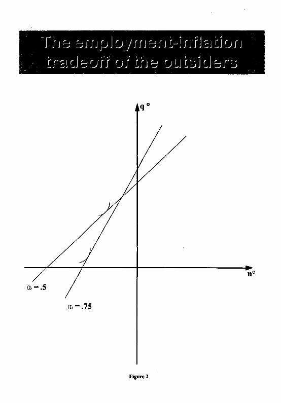
-r! J ~ ~I I J fJ J CJ J I I J ~I J t -.J J I JI J ~J iJ c; I J
ir~1 c.J 3 c;·f f CJ-J t! J ~ CJ u t:.; J ~Jars
OJ= .75
Figurel
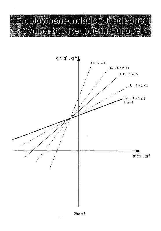
I I
I
I I
I
'. I I
I I
I
I I
I I
I
Figure3
I I
I
0, ClJ =1
' 0, . 5 < ClJ < 1
I, 0, OJ=. 5
. I, .5<CJJ<1
us, . 5 ~a,~ 1 I, OJ =1
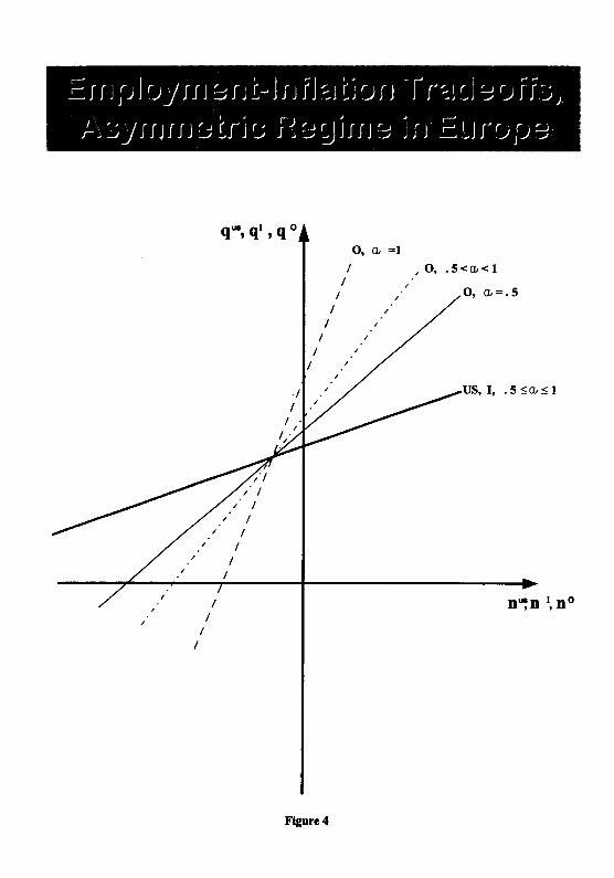
~I I J ;_) J CJ y I I J :; I J i-- J I J 1 J ~J iJ u I J -f r~J c.J :; CJ f 1::.;) ; j ::.; y I I HI J ~ ir J s 5 ~ :; ~ J In :; J n f u r CJ ;_) :;
I I
I I
I
I I
I I
Figure4
0, (], =1
I , 0, . 5 <a,< 1 I
I 0, a,=.5
I
US, I, . S ~a,~ 1