Embed Size (px)
Citation preview

OTR based measurements for ELI-NPGamma Beam Source
Facoltà di Scienze Matematiche Fisiche e NaturaliDottorato di Ricerca in Fisica degli Accelleratori – XXXI Ciclo
CandidateMaco MarongiuID number 1689676
Thesis AdvisorProf. L. Palumbo
Co-AdvisorProf. A. Mostacci
June 2019

Thesis defended on 13 September 2019in front of a Board of Examiners composed by:Prof. D’ Angelo Annalisa (chairman)Prof. Senesi RobertoProf. Antici Patrizio
OTR based measurements for ELI-NP Gamma Beam SourcePh.D. thesis. Sapienza – University of Rome
© 2018, Maco Marongiu.
Author’s email: [email protected]

ii
Contents
List of Symbols iv
1 Introduction 11.1 Layout Characterization . . . . . . . . . . . . . . . . . . . . . 2
1.1.1 Thermal Analysis . . . . . . . . . . . . . . . . . . . . . 21.1.2 Imaging System . . . . . . . . . . . . . . . . . . . . . . 31.1.3 Energy Measurements . . . . . . . . . . . . . . . . . . 4
1.2 Goal of the Thesis . . . . . . . . . . . . . . . . . . . . . . . . 4
2 ELI-NP 52.1 Inverse Compton Scattering . . . . . . . . . . . . . . . . . . . 62.2 ELI-GBS Project . . . . . . . . . . . . . . . . . . . . . . . . . 82.3 ELI-GBS Linac Layout . . . . . . . . . . . . . . . . . . . . . . 11
3 Transition Radiation 163.1 Radiation from Moving Particles . . . . . . . . . . . . . . . . 163.2 Single Particle Transition Radiation . . . . . . . . . . . . . . . 18
3.2.1 Oblique Incidence . . . . . . . . . . . . . . . . . . . . . 203.2.2 Near Field Regime . . . . . . . . . . . . . . . . . . . . 223.2.3 Transition Radiation from Finite Screens . . . . . . . . 24
3.3 Transition Radiation from a Beam . . . . . . . . . . . . . . . . 253.3.1 Coherent Optical Transition Radiation . . . . . . . . . 28
4 Design Issue 304.1 Thermal Analysis . . . . . . . . . . . . . . . . . . . . . . . . . 314.2 ANSYS Numerical Analysis . . . . . . . . . . . . . . . . . . . 364.3 Thermal Stress Evaluation . . . . . . . . . . . . . . . . . . . . 374.4 Optical System Simulation . . . . . . . . . . . . . . . . . . . . 40

Contents iii
4.5 Resolution . . . . . . . . . . . . . . . . . . . . . . . . . . . . . 424.5.1 Calibration Procedure . . . . . . . . . . . . . . . . . . 48
4.6 Photon Counting . . . . . . . . . . . . . . . . . . . . . . . . . 494.7 Transition Radiation as a Diagnostic Tool . . . . . . . . . . . 55
4.7.1 Comparison between YAG and OTR Screens . . . . . . 55
5 Energy Measurements 585.1 Energy Measurement Experiment . . . . . . . . . . . . . . . . 595.2 Energy Measurement Simulations . . . . . . . . . . . . . . . . 635.3 Energy Measurement Design . . . . . . . . . . . . . . . . . . . 69
6 Bunch by Bunch Measurement 716.1 Camera System . . . . . . . . . . . . . . . . . . . . . . . . . . 716.2 Measurements . . . . . . . . . . . . . . . . . . . . . . . . . . . 73
7 Conclusions 77
Bibliography 79
List of Figures 90
List of Tables 99
iv
List of Symbols
β Particle velocity normalized to the speed oflight
7, 19
γ Lorentz Factor 7, 17,63, 73
c Speed of Light in Vacuum (3× 10⁸ m ∗ s−1) 16, 73ε0 Vacuum Dielectric Constant
(8.85× 10⁻¹² F ∗m−1)16
λ Wavelength (m) 22, 63,73
σz Longitudinal RMS Beam Length (m) 26σx,y Transverse RMS Beam Spot Size (m) 28cp Specific Heat (J ∗ kg−1 ∗K−1) 31ρ Material Density (kg ∗m−3) 31Tmelt Material Melting temperature (K) 31ε Material Emissivity 31k Material Thermal Conductivity
(W ∗m−1 ∗K−1)31
αd Material Thermal diffusivity (m2 ∗ s−1) 31σten Material Tensile Strength (MPa) 31αt Material Coefficient of Thermal Linear Expan-
sion (K−1)31
Ey Material Young’s Modulus (GPa) 31∂E/∂z Material Electron Stopping Power (J ∗m−1) 31σsb Stefan Boltzmann Constant
(5.67× 10⁻⁸ W ∗m−2 ∗K−4)37
σVM Von Mises Stress (MPa) 39σa Alternate Stress (MPa) 39

List of Symbols v
σm Mean Stress (MPa) 39σN Goodman Alternate Stress (MPa) 39α Fine Structure Constant (0.007) 50e Elementary Charge (1.6× 10⁻¹⁹ C) 73h Planck’s Constant (6.6× 10⁻³⁴ m2 ∗ kg ∗ s−1) 73

1
Chapter 1
Introduction
Optical Transition Radiation (OTR) monitors are widely used for profilemeasurements at Linacs. The radiation is emitted when a charged particlebeam crosses the boundary between two media with different optical properties,here a thin reflecting screen and vacuum. For beam diagnostic purposes thevisible part of the radiation is used and an observation geometry in backwarddirection is mainly chosen which corresponds to the reflection of virtual photonsat the screen which acts as mirror.
Advantages of OTR are the instantaneous emission process enabling fastsingle shot measurements, and the good linearity (when the coherent componentis negligible); disadvantages are that the process of radiation generation isinvasive (i.e. a screen has to be inserted in the beam path) and that theradiation intensity is much lower in comparison to scintillation screens. Forhigh intensity electron beams the interaction of the beam with the screenmaterial may lead to a screen degradation or even a damage (see section 1.1.1).
The angular distribution of OTR can also be exploited due to the fact thatthe angular distribution possesses characteristic maxima at angles 1/γ with γthe Lorentz factor: from such a measurement the beam energy can be thereforederived (see section 1.1.3).
The Gamma Beam Source (ELI-NP-GBS) machine is an advanced source ofup to ≈20 MeV Gamma Rays based on Compton back-scattering, i.e. collisionof an intense high power laser beam and a high brightness electron beam withmaximum kinetic energy of about 720 MeV. The Linac will provide trains of32 electron bunches in each RF pulse, separated by 16.1 ns; each bunch has acharge of 250 pC .
1.1 Layout Characterization 2
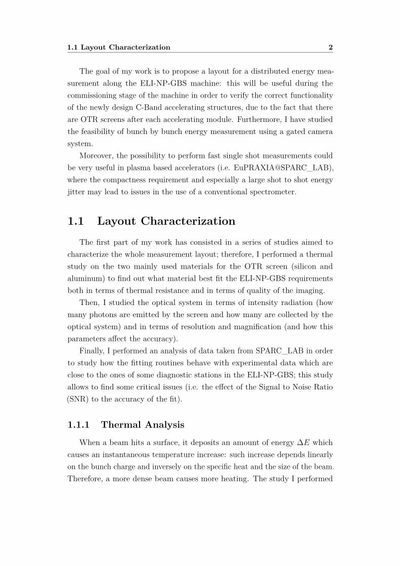
The goal of my work is to propose a layout for a distributed energy mea-surement along the ELI-NP-GBS machine: this will be useful during thecommissioning stage of the machine in order to verify the correct functionalityof the newly design C-Band accelerating structures, due to the fact that thereare OTR screens after each accelerating module. Furthermore, I have studiedthe feasibility of bunch by bunch energy measurement using a gated camerasystem.
Moreover, the possibility to perform fast single shot measurements couldbe very useful in plasma based accelerators (i.e. EuPRAXIA@SPARC_LAB),where the compactness requirement and especially a large shot to shot energyjitter may lead to issues in the use of a conventional spectrometer.
1.1 Layout Characterization
The first part of my work has consisted in a series of studies aimed tocharacterize the whole measurement layout; therefore, I performed a thermalstudy on the two mainly used materials for the OTR screen (silicon andaluminum) to find out what material best fit the ELI-NP-GBS requirementsboth in terms of thermal resistance and in terms of quality of the imaging.
Then, I studied the optical system in terms of intensity radiation (howmany photons are emitted by the screen and how many are collected by theoptical system) and in terms of resolution and magnification (and how thisparameters affect the accuracy).
Finally, I performed an analysis of data taken from SPARC_LAB in orderto study how the fitting routines behave with experimental data which areclose to the ones of some diagnostic stations in the ELI-NP-GBS; this studyallows to find some critical issues (i.e. the effect of the Signal to Noise Ratio(SNR) to the accuracy of the fit).
1.1.1 Thermal Analysis
When a beam hits a surface, it deposits an amount of energy ∆E whichcauses an instantaneous temperature increase: such increase depends linearlyon the bunch charge and inversely on the specific heat and the size of the beam.Therefore, a more dense beam causes more heating. The study I performed
1.1 Layout Characterization 3
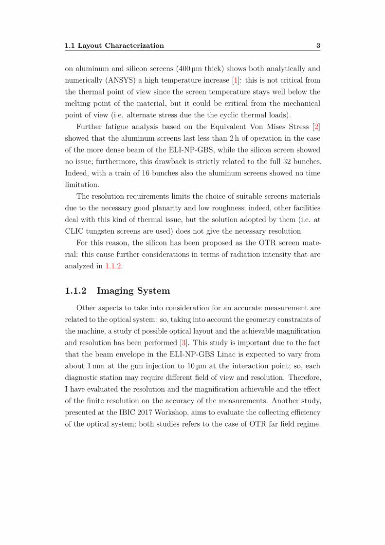
on aluminum and silicon screens (400 µm thick) shows both analytically andnumerically (ANSYS) a high temperature increase [1]: this is not critical fromthe thermal point of view since the screen temperature stays well below themelting point of the material, but it could be critical from the mechanicalpoint of view (i.e. alternate stress due the the cyclic thermal loads).
Further fatigue analysis based on the Equivalent Von Mises Stress [2]showed that the aluminum screens last less than 2 h of operation in the caseof the more dense beam of the ELI-NP-GBS, while the silicon screen showedno issue; furthermore, this drawback is strictly related to the full 32 bunches.Indeed, with a train of 16 bunches also the aluminum screens showed no timelimitation.
The resolution requirements limits the choice of suitable screens materialsdue to the necessary good planarity and low roughness; indeed, other facilitiesdeal with this kind of thermal issue, but the solution adopted by them (i.e. atCLIC tungsten screens are used) does not give the necessary resolution.
For this reason, the silicon has been proposed as the OTR screen mate-rial: this cause further considerations in terms of radiation intensity that areanalyzed in 1.1.2.
1.1.2 Imaging System
Other aspects to take into consideration for an accurate measurement arerelated to the optical system: so, taking into account the geometry constraints ofthe machine, a study of possible optical layout and the achievable magnificationand resolution has been performed [3]. This study is important due to the factthat the beam envelope in the ELI-NP-GBS Linac is expected to vary fromabout 1 mm at the gun injection to 10 µm at the interaction point; so, eachdiagnostic station may require different field of view and resolution. Therefore,I have evaluated the resolution and the magnification achievable and the effectof the finite resolution on the accuracy of the measurements. Another study,presented at the IBIC 2017 Workshop, aims to evaluate the collecting efficiencyof the optical system; both studies refers to the case of OTR far field regime.
1.2 Goal of the Thesis 4
1.1.3 Energy Measurements
The OTR angular distribution of a single particle, also called Single ParticleFunction (SPF), has a center minimum equal to zero, and two maxima; thedistance of these two maxima is inversely proportional to the particle energy.However, when the beam angular distribution is observed, also the beamdivergence need to be taken into account: the main effect is to shift up theminimum from zero to a value which could be close to the maximum.
Assuming a gaussian distribution of the beam divergence, one can convolutethis distribution with the SPF and retrieve a fitting equation that can allowto measure beam energy and beam divergence. I have performed this analysisusing data taken from the SPARC_LAB facility in order to evaluate theaccuracy of the measurement in different working conditions (i.e. single shotmeasurement, different values of energy, charge and divergence). The resultshave been presented at the EAAC Workshop.
Another possible measurement could be the energy measurement of aplasma accelerated beam (i.e. EuSPARC@SPARC_LAB) thanks to the singleshot possibility of this measurement technique: the large energy jitter, indeed,could lead to inaccurate measurement with conventional techniques. In thiscase, however, one must take into account the contribution given by the energyspread.
1.2 Goal of the Thesis
The main goal of the thesis is to propose a layout for a distributed energymeasurement along the ELI-NP-GBS machine. In order to correctly performthe measurements, few improvements need to be done to the optical layout:for instance, by adopting a specific optical layout one could increase theresolution or the magnification or the depth of field or, more in general, theoverall performance of the diagnostic system.I performed these studies alsowith simulation software like Zemax.
Furthermore, in order to perform the measurement of a single bunch of thetrain using a gating camera and an intensifier (i.e. “Hamamatsu Orca-Flash4”),I have characterized the camera in order to find the optimum gain value foreach working point to avoid a bad SNR or saturation. Both the situationscould compromise the measurement accuracy.
5
Chapter 2
ELI-NP
Recent developments in particle accelerators and lasers technology openednew perspectives for the realization of new X and γ ray sources throughelectron-photon collision. These sources are based on the inverse Comptonscattering effect, in which a high brightness electron beam scatters an intensehigh power laser beam, converting optical photons (Eph ≈ eV) into energeticphotons ranging from KeV to MeV.
The idea of using Compton scattering to generate a high energy X-Rayor γ-Ray beam was first proposed in 1963 by Milburn [4] and Arutyunian [5].The LADON project [6] has been the first facility to produce a monochromaticpolarized gamma beam exploiting the collision of a laser with the electronsfrom the ADONE storage ring [7] in Frascati. Nowadays several test facilities,that generate γ-Ray beams by means of Compton scattering are present indifferent laboratories worldwide [8, 9, 10, 11, 12, 13], together with newlyconceived user facilities [14, 15, 16, 17]. This is true both for X-Ray sources,which are primarily used for advanced imaging techniques, and for the γ-Raysources used for research in nuclear physics and industrial purposes. Theyfound their natural interest in imaging and nuclear fundamental physics, buttheir potential application range extends to a large number of fields: medicine,biology, material science, cultural heritage, national security and high energyphysics.
Photon beams generated by Compton scattering have been successfullyused for the implementation of biological computer aided imaging techniques,like for instance phase-contrast tomography at the Munich Compact LightSource [15, 18]. This has been possible thanks to small round source spot size,

2.1 Inverse Compton Scattering 6
high spatialand temporal resolution, and the quasi-monochromaticity typicalof these sources. Moreover, with respect to the conventional X-Ray tubes, theabsence of low energy tails in the photon spectrum, allows edge enhancementwith an overall improvement in the image contour visibility. In particular inthe medical field, mammography with mono-chromatic X-Rays at 20 KeV hasbeen proven far superior in signal to noise ratio with respect to conventionalmammographic tubes, with a considerably lower radiation dose to the tissue.
The generation of photons in the gamma range (Eph > 1 MeV) is particu-larly interesting for nuclear physics applications, e.g. the Nuclear ResonanceFluorescence technique [19, 20] based on the nuclear absorption and subsequentemission of high energy photons. This technique provides a versatile methodof non-destructive analysis of both radioactive and stable nuclides. Therefore,it finds application for nuclear waste remote sensing and diagnostics, specialnuclear material recognition for national security but also in isotope sensitiveimaging for medical and cultural heritage purposes. Moreover, several researchfields in nuclear physics and astrophysics dealing with fundamental nuclearstructure studies such as nucleo-synthesis, clustering phenomena in light nuclei,photo-disintegration cross-sections measurements and photo-fission phenomenawill be possible with such advanced gamma sources.
2.1 Inverse Compton Scattering
The physics of the inverse Compton scattering effect has been studiedextensively and can be described through two different models [21]: classicalmodel and a linear quantum model. In the former the laser pulse field actsas an electromagnetic undulator: like in a Free Electron Laser (FEL), theelectrons oscillating in this field produce spontaneous emission radiation. Thismodel considers all the collective effects (multi-photon absorption/emission)explaining the beam-laser pulse interaction, but it does not conserve energy andmomentum. In order to take into account the quantum effects and how theyimpact on the quality of the produced secondary beam, the linear quantumapproach is used. It is based on the relativistic kinematics and allows to predictthe final characteristics and performances for a high energy Compton source.
As reported in [14], in the laboratory frame shown in Figure 2.1 the energyEγ of the scattered γ-Ray, propagating in the direction given by the polar

2.1 Inverse Compton Scattering 7
Figure 2.1. Sketch of Compton scattering of an electron and a photon in thelaboratory frame: the electron is moving along the ze direction while the incidentphoton is propagating along the direction given by the polar angle θi and theazimuthal angle φi. The collision happens at the origin of the coordinate system,and the scattered γ ray propagates in the direction given by the polar angle θfand the azimuthal angle φf . θp is the angle between the momenta of incidentand scattered photons, while the electron after the collision is not shown in thefigure.
angle θf , can be expressed by:
Eγ = (1− β cos θi)Ep1− β cos θf + (1− cos θp)Ep/Ee
, (2.1)
where β= v/c is the ratio of the incident electron velocity relative to the speedof light, Ee and Ep are the energy of the electron and optical photon beforescattering, θi is the angle between the momenta of the incident photon and theelectron and θp is the angle between the momenta of the incident and scatteredphotons.
In case of head-on collision (θi = π and θp = π − θf ) and ultra-relativisticelectron, the photon is scattered into a cone with a half-opening angle equal tothe inverse of the Lorentz factor γ along the direction of the incident electron.For a small scattering angle, the Equation 2.1 can be simplified to:
Eγ ≈4γ2Ep
1 + γ2θ2f + 4γ2Ep/Ee
, (2.2)
in which the last term in the denominator accounts for the so called electronrecoil effect and it is responsible for the correct energy and momentum conser-vation in the scattering reaction. This term, that affects the performances of
2.2 ELI-GBS Project 8
the emitted photon beam, is negligible for X-Ray Thomson Sources, while it issmall but not negligible for higher energy Compton Sources, and becomes thedominant term for deep Compton Sources. In general, it is possible to identifythree different regimes:
• Thomson elastic regime: negligible electron recoil;
• Quasi-elastic Compton regime: small but not negligible recoil;
• Quantum Compton regime: dominant electron recoil.
As shown by Equation 2.2, the photon energy gain factor in the inverseCompton scattering mainly depends on the energy of the colliding electronbeam. This beam can be generated by a normal conducting linear accelerator(Linac), a storage ring or a superconducting Linac. Compton sources areeasily tunable and their photon beam energies can be extended to covera wide range from soft X-Ray to very high energy γ-Ray. Due to a highenergy gain factor, the Compton sources are considered the most effective“photon accelerators”, able to produce high power radiation with a requiredelectron beam energy, dimensions and costs significantly lower than those of asynchrotron light source. Furthermore, secondary photons emitted by inverseCompton scattering present an energy-angle correlation. Hence, by using acollimation system, it is possible to obtain a quasi-monochromatic photonbeam, while the forward focusing ensures high spectral densities in smallbandwidths. Compared with a Bremsstrahlung beam which is characterizedby a broadband spectrum, a Compton beam is narrowly peaked around thedesired energy. Another important feature is the preservation of the laserpolarization in the scattered photons. Hence, the photon beams produced withthis scheme can be highly polarized, and their polarization is controlled by theone of the incident photon beam.
2.2 ELI-GBS Project
A new Compton source operating in the gamma energy range (0.2-19.5 MeV)is presently under construction in the framework of the Extreme Light Infras-tructure Nuclear Physics Gamma Beam System (ELI-NP-GBS) project. TheELI-NP-GBS project [22, 23, 24] consists in the realization and commissioning

2.2 ELI-GBS Project 9
of a γ-Ray source that will be hosted in Magurele, near Bucharest (Romania).The design of this machine has been performed by the EuroGammaS asso-ciation [25] which gathers academic and research institutions together withcommercial companies: Istituto Nazionale di Fisica Nucleare, Università diRoma “La Sapienza”, the Centre National de la Recherche Scientifique, ACPS.A.S., Alsyom S.A.S., Comeb Srl and ScandiNova Systems AB. This projecthas been developed in the framework of the ELI project, born from the collab-oration of 13 European countries and aims at the creation of an internationallaser research infrastructure that will host high level research on ultra-highintensity laser, laser-matter interaction and secondary light sources. Its goal isto reach pulse peak power and brightness beyond the current state of the artby several orders of magnitude. Because of its unique properties, this multi-disciplinary facility will provide new opportunities to study the fundamentalprocesses unfolded during light-matter interaction. ELI will be implementedas a distributed research infrastructure based initially on 3 specialized andcomplementary facilities (or pillars):
• ELI Beamlines (Prague (Czech Republic)): High Energy BeamScience pillar devoted to the development and usage of dedicated beamlines with ultra short pulses of high energy radiation and particles reachingalmost the speed of light.
• ELI Attosecond (Szeged (Hungary)): Attosecond Laser Sciencepillar designed to conduct temporal investigation of electron dynamics inatoms, molecules, plasmas and solids at attosecond scale (1× 10⁻¹⁸ s).
• ELI-NP (Magurele (Romania)): Laser-based Nuclear Physics pillarwill generate radiation and particle beams with much high energy andbrilliance suited to studies of nuclear and fundamental processes.
At the ELI-NP pillar, the ELI-NP-GBS is foreseen as a major componentof the infrastructure, aiming at producing extreme γ-Ray beams for nuclearphysics and photonics experiments characterized by unprecedented perfor-mances in terms of monochromaticity, brilliance, spectral density, tunabilityand polarization. The ELI-NP source [24, 26] is a machine based on the collisionof an intense high power Yb:Yag J-class laser and an high brightness electronbeam with a tunable energy produced by a normal conducting Linac. Referring
2.2 ELI-GBS Project 10
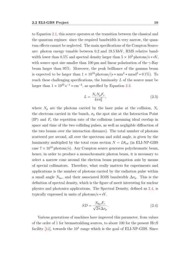
to Equation 2.1, this source operates at the transition between the classical andthe quantum regimes: since the required bandwidth is very narrow, the quan-tum effects cannot be neglected. The main specifications of the Compton Sourceare: photon energy tunable between 0.2 and 19.5 MeV, RMS relative band-width lower than 0.5% and spectral density larger than 5× 10³ photons/s ∗ eV,with source spot size smaller than 100 µm and linear polarization of the γ-Raybeam larger than 95%. Moreover, the peak brilliance of the gamma beamis expected to be larger than 1× 10¹⁹ photons/(s ∗mm2 ∗mrad2 ∗ 0 1%). Toreach these challenging specifications, the luminosity L of the source must belarger than 1× 1035 s−1 ∗ cm−2, as specified by Equation 2.3.
L = NeNpFr4πσ2
0, (2.3)
where Np are the photons carried by the laser pulse at the collision, Ne
the electrons carried in the bunch, σ0 the spot size at the Interaction Point(IP) and Fr the repetition rate of the collisions (assuming ideal overlap inspace and time of the two colliding pulses, as well as negligible diffraction ofthe two beams over the interaction distance). The total number of photonsscattered per second, all over the spectrum and solid angle, is given by theluminosity multiplied by the total cross section N = Lθtot (in ELI-NP-GBScase 7× 10¹⁰ photons/s). Any Compton source generates polychromatic beam,hence, in order to produce a monochromatic photon beam, it is necessary toselect a narrow cone around the electron beam propagation axis by meansof special collimators. Therefore, what really matters for experiments andapplications is the number of photons carried by the radiation pulse withina small angle Nbw, and their associated RMS bandwidth ∆νp. This is thedefinition of spectral density, which is the figure of merit interesting for nuclearphysics and photonics applications. The Spectral Density, defined as 2.4, istypically expressed in units of photons/s ∗ eV.
SD = NbwFr√2π∆νp
. (2.4)
Various generations of machines have improved this parameter, from valuesof the order of 1 for bremsstrahlung sources, to about 100 for the present HiγSfacility [14], towards the 104 range which is the goal of ELI-NP-GBS. Since
2.3 ELI-GBS Linac Layout 11
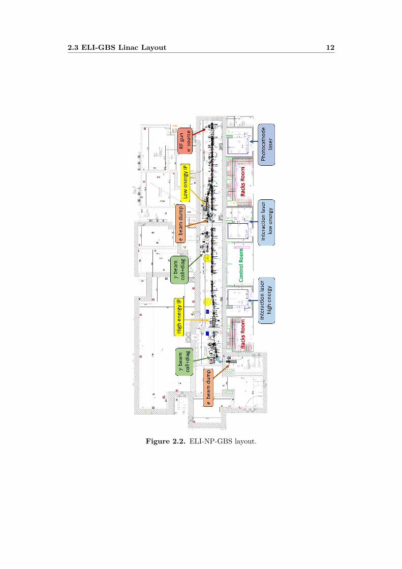
the laser pulse carries about 1018 photons at the IP, but only a maximum of107 photons are scattered at each collision (in other words the electron beam isalmost transparent to the laser pulse), the laser pulse can be “recycled” bringingit back to a new collision at the same IP with a new incoming electron bunch.To recirculate the laser pulse, an advanced and innovative laser re-circulatorhas been developed and it is presently under test. A full description of this newoptical device can be found in [27]. To achieve this outstanding performancethe laser pulse needs to be recirculated 32 times at the IP and consequentlythe Linac will accelerate 32 electron bunches (separated by 16.1 ns) within thesame RF bucket, with a repetition rate of 100 Hz. The final parameters of thegamma beam of ELI-NP-GBS are summarized in Table 2.1 and the layout ofthe entire building is shown in Figure 2.2.
Table 2.1. Main parameters of the ELI-NP-GBS Gamma beam.
Energy (MeV) 0.2-19.5Spectral Density (photon/s ∗ eV) 0.8-4× 10⁴
Bandwidth RMS (%) ≤ 0.5Photons per Pulse ≤2.6× 10⁵
Photons per Second ≤8.3× 10⁸
RMS Size (µm) 10-30RMS Divergence (µrad) 25-200Peak Brilliance (photon/s ∗mm2 ∗mrad2 ∗ 0 1%) 1× 10²⁰-1× 10²³
RMS Pulse Length (ps) 0.7-1.5Linear Polarization (%) > 99
2.3 ELI-GBS Linac Layout
In order to reach these challenging performances innovative and advancedcomponents have been developed specifically for this machine. In order toaccelerate the multi-bunch electron beam, the ELI-NP-GBS adopts an S-band(2856 MHz) photo-injector coupled to a C-band (5712 MHz) Radio-Frequency(RF) Linac capable to bring the electron beam up to an energy of 740 MeVwith outstanding beam quality [28]: normalized RMS emittance in both planesbelow 0.5 mm ∗mrad and energy spread below 0.1%; in Tables 2.2 and 2.3 aresummarized the main required parameters of the electron beam. In order toincrease as much as possible the number of collision per second, the Linac will
2.3 ELI-GBS Linac Layout 12
Figure 2.2. ELI-NP-GBS layout.

2.3 ELI-GBS Linac Layout 13
Table 2.2. Main parameters of the ELI-NP-GBS electron beam.
Energy (MeV) 75-740RMS Energy Spread (%) 0.04-0.1Bunch Charge (pC) 25-400Bunch per Pulse 32Bunch Separation (ns) 16.1Bunch length (µm) 100-400Normalized Emittance (mm ∗mrad) 0.4Repetition Rate (Hz) 100
work at 100 Hz repetition rate and in multi-bunch scheme; these requirementshave direct impact on the design of the accelerating structures and in theoverall RF system.
Table 2.3. Main parameters of the ELI-NP-GBS laser beam.
Pulse Energy (J) 0.2-0.4Photon Energy (eV) 2.4Wavelength (nm) 515RMS Pulse length (ps) 1.5Focal Spot Size w0 (µm) 28RMS Bandwidth ≤0.1Collision Angle (°) 172Repetition Rate (Hz) 100Recirculator Rate per Laser Pulse 32
To realize a reliable and compact machine a hybrid S/C-band schemehas been chosen: the combination of C-band acceleration with an S-bandinjector allows to obtain good performance in terms of beam quality [29]. Theinjector is derived from the one of SPARC_LAB Linac [30] at INFN Frascatilaboratories and is composed by one 1.6 cell RF gun with copper photo-cathodeand emittance compensation solenoid, followed by two SLAC-type 3 m longTravelling Wave (TW) sections To compensate space charge effect in the gunregion and to reduce the bunch length, the velocity bunching technique [31] isapplied in the first accelerating section placed after the gun: this techniqueconsists in injecting a non-relativistic beam in an RF structure with a phasenear the zero crossing of the acceleration field. In this way, the beam slips backup to the acceleration phase undergoing a quarter of synchrotron oscillationand is chirped and compressed; in the ELI-NP-GBS case, a compression
2.3 ELI-GBS Linac Layout 14
factor below 3 in the first accelerating section allows injecting into the C-bandbooster a beam that is short enough to reduce the final energy spread, avoidingalso emittance degradation. In the first accelerating section, the transverseemittance dilution is controlled by a solenoid embedded to the RF compressor;the C-band booster comprises 12 TW C-band room temperature acceleratingstructures, downstream of the S-band photo-injector.
Two beamlines are planned to deliver the electron beam at the two ComptonIPs: one at low energy (Ee = 312 MeV) and one at high energy (up to 740 MeV).Downstream the injector and the first four C-band structures, a dogleg withtwo dipoles provide an off axis deviation towards the low energy interactionpoint; at the end of the Linac a second dogleg drives the beam to the highenergy Compton IP. After each interaction point the electron beam is driventhrough dipoles towards the low and high energy dump, while the Comptonradiation proceeds in straight direction towards the collimator and the γ-Raydiagnostics (Compton spectrometer, calorimeter, etc.) in the experimentalrooms.
The beam characterization is essential to properly match the electron beamcoming from the RF Linac to provide the required phase space orientation atthe IP. The beam envelope is captured in several positions along the machineand in particular at the gun exit, at the low and high energy Linac entranceand exit and at the IPs. All the 23 monitoring positions are equipped with botha YAG:Ce and an Optical Transition Radiation (OTR) screen; the detectorsare the Basler “Scout scA640-70gm” CCD camera [32]. In case of some morecrucial measurements, a Hamamatsu “Orca-Flash 4” gated camera with anintensifier [33] can be used; more details on the optic system will be shown inthe Chapter 4. The imaging on the screen mounted at the gun exit is used forthe beam energy measurement, provided by means of the beam deflection asteerer (horizontal or vertical) upstream the screen, and to center the beam onthe photo cathode. The longitudinal phase space characterization is obtainedusing a S-band RF deflecting cavity [34] coupled with a dipole in two mainlocations: downstream the first C-band cavity of the low energy Linac andupstream the first C-band cavity of the high energy Linac. The 6D phase spacecharacterization is completed in these places with the emittance measurementsby means of the quadrupole scan technique. The latter can be also done at eachstraight-on section of the Linac to keep under control the eventual emittance

2.3 ELI-GBS Linac Layout 15
dilution. Four beam current monitors are placed at the gun exit and all alongthe machine in order to optimize the beam charge transport up to the IP. Thecurrent measurements at the gun exit together with a RF injection phase scanenables the identification of the proper injection phase needed to maximize thebeam energy gain as indicated by the beam dynamics simulations. The beamtrajectory is measured by 29 stripline beam position monitors (BPM) all alongthe machine and, at the interaction region entrance and exit, by cavity BPMswhich resolution is of the order of 2 µm instead of 10 µm of the stripline BPMs.Finally, beam loss monitors are placed all along the machine.
16
Chapter 3
Transition Radiation
This Chapter is a description of the theory behind the transition radiation:at first only the case of a single electron is considered and then, the case of aparticle beam is treated (Section 3.3).
For the single particle case, different situations have been considered: theangle of incidence of the particle in Section 3.2.1, the distance between detectorand the source of radiation in Section 3.2.2 (Far and Near Field) and the screendimension in Section 3.2.3.
For a particle beam case, also the coherent radiation has been treated inSection 3.3.1
However, in the ELI-NP-GBS case, the radiation expected will be incoherentand in the far field; hence, in the next Chapters, only the issues related to thistype of radiation will be considered.
3.1 Radiation from Moving Particles
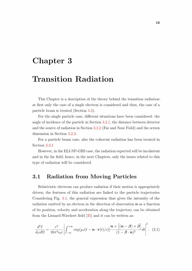
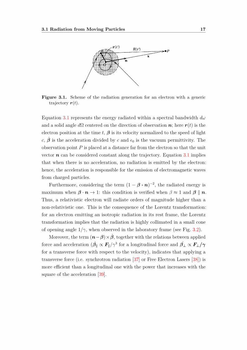
Relativistic electrons can produce radiation if their motion is appropriatelydriven; the features of this radiation are linked to the particle trajectories.Considering Fig. 3.1, the general expression that gives the intensity of theradiation emitted by an electron in the direction of observation n as a functionof its position, velocity and acceleration along the trajectory can be obtainedfrom the Lienard-Wiechert field [35] and it can be written as:
d2I
dωdΩ = e2
16π3ε0c
∣∣∣∣∣∣∫ +∞
−∞exp[ω(t− n · r(t)/c)]
n×[(n− β)× β
](1− β · n)2 dt
∣∣∣∣∣∣2
. (3.1)
3.1 Radiation from Moving Particles 17
Figure 3.1. Scheme of the radiation generation for an electron with a generictrajectory r(t).
Equation 3.1 represents the energy radiated within a spectral bandwidth dωand a solid angle dΩ centered on the direction of observation n; here r(t) is theelectron position at the time t, β is its velocity normalized to the speed of lightc, β is the acceleration divided by c and ε0 is the vacuum permittivity. Theobservation point P is placed at a distance far from the electron so that the unitvector n can be considered constant along the trajectory. Equation 3.1 impliesthat when there is no acceleration, no radiation is emitted by the electron:hence, the acceleration is responsible for the emission of electromagnetic wavesfrom charged particles.
Furthermore, considering the term (1 − β · n)−2, the radiated energy ismaximum when β · n→ 1: this condition is verified when β ≈ 1 and β ‖ n.Thus, a relativistic electron will radiate orders of magnitude higher than anon-relativistic one. This is the consequence of the Lorentz transformation:for an electron emitting an isotropic radiation in its rest frame, the Lorentztransformation implies that the radiation is highly collimated in a small coneof opening angle 1/γ, when observed in the laboratory frame (see Fig. 3.2).
Moreover, the term (n−β)×β, together with the relations between appliedforce and acceleration (β‖ ∝ F‖/γ3 for a longitudinal force and β⊥ ∝ F⊥/γfor a transverse force with respect to the velocity), indicates that applying atransverse force (i.e. synchrotron radiation [37] or Free Electron Lasers [38]) ismore efficient than a longitudinal one with the power that increases with thesquare of the acceleration [39].

3.2 Single Particle Transition Radiation 18
Figure 3.2. Scheme of the Lorentz transformation. Picture taken from [36].
Figure 3.3. Scheme of the transition radiation generation. Picture taken from[46].
3.2 Single Particle Transition Radiation
The Transition Radiation (TR) happens when the moving particle crossesthe boundary between two media with different dielectric constant. The elec-tromagnetic field carried by the particle changes abruptly upon the transitionfrom one medium to the other; to satisfy the boundary conditions for theelectric and the magnetic field vectors, one has to add two radiation fields: onepropagating in backward direction and the other in forward direction. Thisradiation is called transition radiation and it was first theorized by Ginzburgand Frank [40] in 1946. The analytical derivation of the equation of radiationis based on the solution of the Maxwell’s equations [41]: some authors use theretarded potential method [42, 43]; other authors propose the use of the Hertzpotential [44] or the image charge method [45].
At the boundary, therefore, two radiation beams are generated: one prop-agates in the first medium (backward transition radiation) and the otherpropagates in the second medium (forward TR) as shown in Fig. 3.3: solving

3.2 Single Particle Transition Radiation 19
the Maxwell’s equations one can derive the equations for the two radiations [41].
[dI2
SP (n, ω)dωdΩ
]1
= e2β2√ε1 sin2 θ1 cos2 θ1
4π3cε0
∣∣∣∣∣∣∣∣(ε2 − ε1)
(1− β2ε1 + β
√ε2 − ε1 sin2 θ1
)(1− β2ε1 cos2 θ1)
(1 + β
√ε2 − ε1 sin2 θ1
)∣∣∣∣∣∣∣∣2
×
∣∣∣∣∣∣ 1ε2 cos θ1 +
√ε1ε2 − ε21 sin2 θ1
∣∣∣∣∣∣2
. (3.2)
Equation 3.2 refers to the backward radiation and Equation 3.3 refers to theforward one: the subscript indicates the medium. It is interesting to notethat one equation can be obtained from the other with a permutation of thesubscripts and substituting β with −β.
[dI2
SP (n, ω)dωdΩ
]2
= e2β2√ε2 sin2 θ2 cos2 θ2
4π3cε0
∣∣∣∣∣∣∣∣(ε1 − ε2)
(1− β2ε2 − β
√ε1 − ε2 sin2 θ2
)(1− β2ε2 cos2 θ2)
(1− β
√ε1 − ε1 sin2 θ2
)∣∣∣∣∣∣∣∣2
×
∣∣∣∣∣∣ 1ε1 cos θ2 +
√ε1ε2 − ε22 sin2 θ2
∣∣∣∣∣∣2
. (3.3)
It is also interesting to note that the radiation is proportional to |ε2 − ε1|2
and, for non relativistic particles, to the square of the velocity; in general, thedielectric constant is a function of the frequency.
In most practical case for beam diagnostics in a accelerator, the equationscan be simplified: indeed, in a particle accelerator, the transition happensbetween vacuum and a media (i.e. aluminum) for the backward transitionradiation and between a media and the vacuum for the forward radiation. Inthe case of relativistic particles, the Equations 3.4 and 3.5 can be reducedto [47]:
[dI2
SP (n, ω)dωdΩ
]1
= e2
4π3cε0
sin2 θ(1γ2 + sin2 θ
)2
∣∣∣∣∣√ε2 − 1√ε2 + 1
∣∣∣∣∣2
, (3.4)
[dI2
SP (n, ω)dωdΩ
]2
= e2
4π3cε0
sin2 θ(1γ2 + sin2 θ
)2 . (3.5)
Equation 3.4 differs from Equation 3.5 only for a term which is dependenton the dielectric constant of the medium that represents the reflectivity of

3.2 Single Particle Transition Radiation 20
the material; furthermore, Equation 3.5 is the well known Ginzburg-Frankformula [40].
-10 -5 0 5 10
(rad)
0
0.2
0.4
0.6
0.8
1
I (a
.u.)
=20
=40
=60
=80
=100
1/
Figure 3.4. Transition Radiation for different energy: the intensities are normalizedto the highest intensity value; the gray dot-dashed line represents the valueθM = 1/γ where the peaks of the distributions are located. The blue linerepresents a γ equal to 20, the red one a γ equal to 40, the green line 60, theblack one 80 and the cyan line represents a γ equal to 100. The peak of theintensity scales with the square of the energy.
In the highly relativistic regime (γ ≥ 20) we can consider very small anglesθ, hence we can approximate sin θ with the angle itself: it is easy to verify thatthe peaks of the distribution are placed at θM = ±1/γ (see Figure 3.4).
3.2.1 Oblique Incidence
We have assumed thus far a normal incidence of the particle trough thesurface; however, a typical use of transition radiation as a diagnostic toolrequires a 45° tilt of the TR screen (see Fig. 3.3). Hence, it is important toevaluate the effect of an oblique incidence on the radiation. The issue of theradiation produced by a particle crossing an interface at oblique incidencewas extensively investigated by Ashley [44] and Pafomov [48]: the derivationof the equations for the oblique incidence is rather cumbersome. In the casewhere one of the medium is vacuum, the equations can be written [41] as in
3.2 Single Particle Transition Radiation 21
Equation 3.6 and 3.7:I‖SP (n, ω)dωdΩ
2
= e2β2z cos2 θz|1− ε|2
4π3ε0c[(1− βx cos θx)2 − β2z cos2 θz]2 sin2 θz
×
∣∣∣∣∣∣(1− βz√ε− sin2 θz − β2
z − βx cos θx) sin2 θz + βxβz cos θx√ε− sin2 θz
(1− βx cos θx − β√ε− sin2 θz)(
√ε− sin2 θz + ε cos θz)
∣∣∣∣∣∣2
,
(3.6)
[dI⊥SP (n, ω)dωdΩ
]2
= e2β2xβ
4z cos2 θy cos2 θz|1− ε|2
4π3ε0c[(1− βx cos θx)2 − β2z cos2 θz] sin2 θz
×
∣∣∣∣∣∣ 1(1− βx cos θx − βz
√ε− sin2 θz)(
√ε− sin2 θz + cos θz)
∣∣∣∣∣∣2
.
(3.7)
In order to obtain the backward radiation, one must permute the subscript1 and 2 and substitute βz with −βz; the radiation is here decomposed inthe parallel (I‖) and perpendicular (I⊥) polarizations with respect to theradiation plane (the plane defined by the photon direction and the normal tothe reflecting surface). The incidence direction is determined by the valuesβz = β cosψ and βx = β sinψ; and the direction of radiation is determined bythe directing cosine of the wave vector k. The directing cosine can be writtenas cos θx = sin θ1,2 cosψ; cos θy = sin θ1,2 sinψ; cos θz = cos θ1,2.
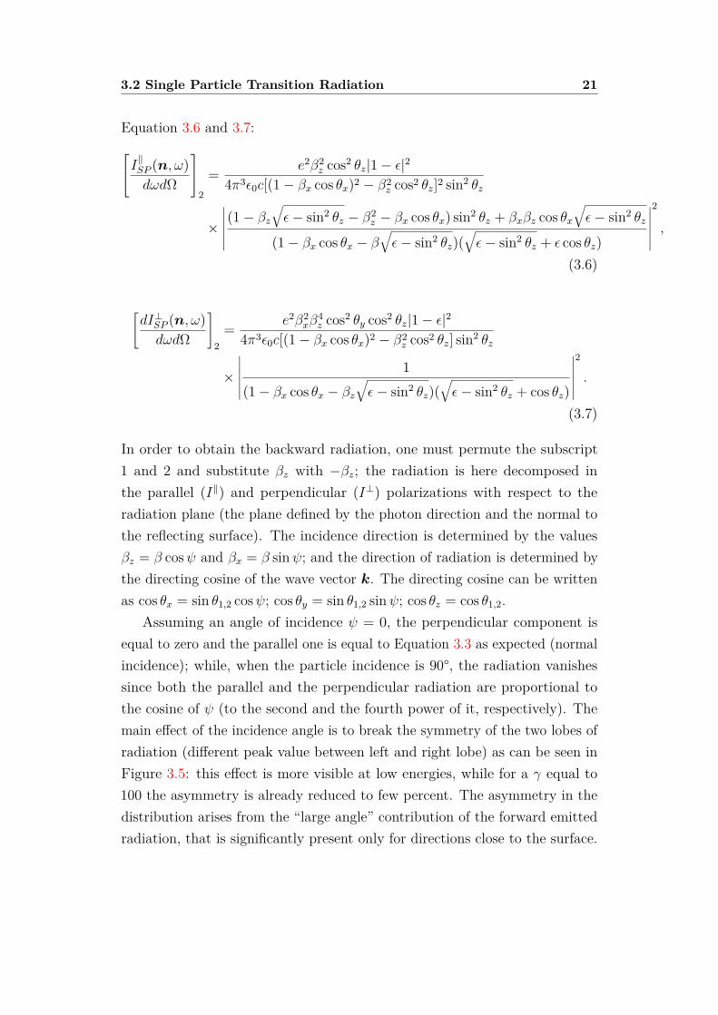
Assuming an angle of incidence ψ = 0, the perpendicular component isequal to zero and the parallel one is equal to Equation 3.3 as expected (normalincidence); while, when the particle incidence is 90°, the radiation vanishessince both the parallel and the perpendicular radiation are proportional tothe cosine of ψ (to the second and the fourth power of it, respectively). Themain effect of the incidence angle is to break the symmetry of the two lobes ofradiation (different peak value between left and right lobe) as can be seen inFigure 3.5: this effect is more visible at low energies, while for a γ equal to100 the asymmetry is already reduced to few percent. The asymmetry in thedistribution arises from the “large angle” contribution of the forward emittedradiation, that is significantly present only for directions close to the surface.
3.2 Single Particle Transition Radiation 22
-5 0 5
(rad)
0
0.2
0.4
0.6
0.8
1
I (a
.u.)
Figure 3.5. Theoretical backward transition radiation patterns at different energiesof the incident electron (incidence angle of 45°). The blue curve represents anelectron energy of 10 MeV; the red line represents the case of 100 MeV and thegreen line represents an energy of 1 GeV.
3.2.2 Near Field Regime
We assume that, as stated before, the distance between the observationpoint and the source of radiation must be long enough (it is the so calledFar Field regime). More precisely, the distance must be much larger than theformation zone in vacuum (sometimes called also coherence length) which canbe defined as the length for which the phase difference between radiation fieldand particle field is equal to 1 rad.
The analytical evaluation of the formation zone can be obtained using theLandau-Lifshits classical method [49]. At relativistic energies, the formationzone can be written as γ2λ/π with λ the observation wavelength [50].
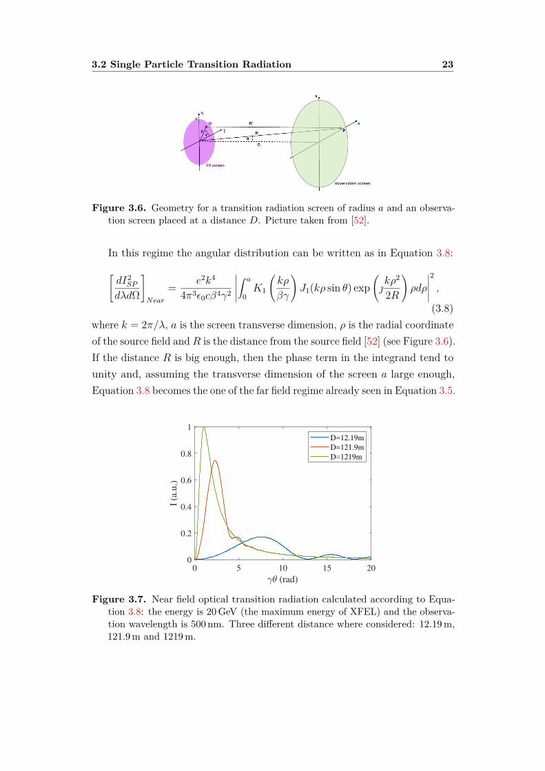
In the ELI-NP-GBS case, with beam energies in the order of hundreds ofMeV and observation wavelength in the optical spectrum, the far field regimeis reached just after few millimiters; however, when the beam energy is on theorder of the GeV like, for instance, at XFEL [51] where it reaches 20 GeV, theformation zone is on the order of hundreds of meters (see Figure 3.7). Thismeans that the transition radiation diagnostics must be performed in a regimedifferent from the far field that is called near field regime.
3.2 Single Particle Transition Radiation 23
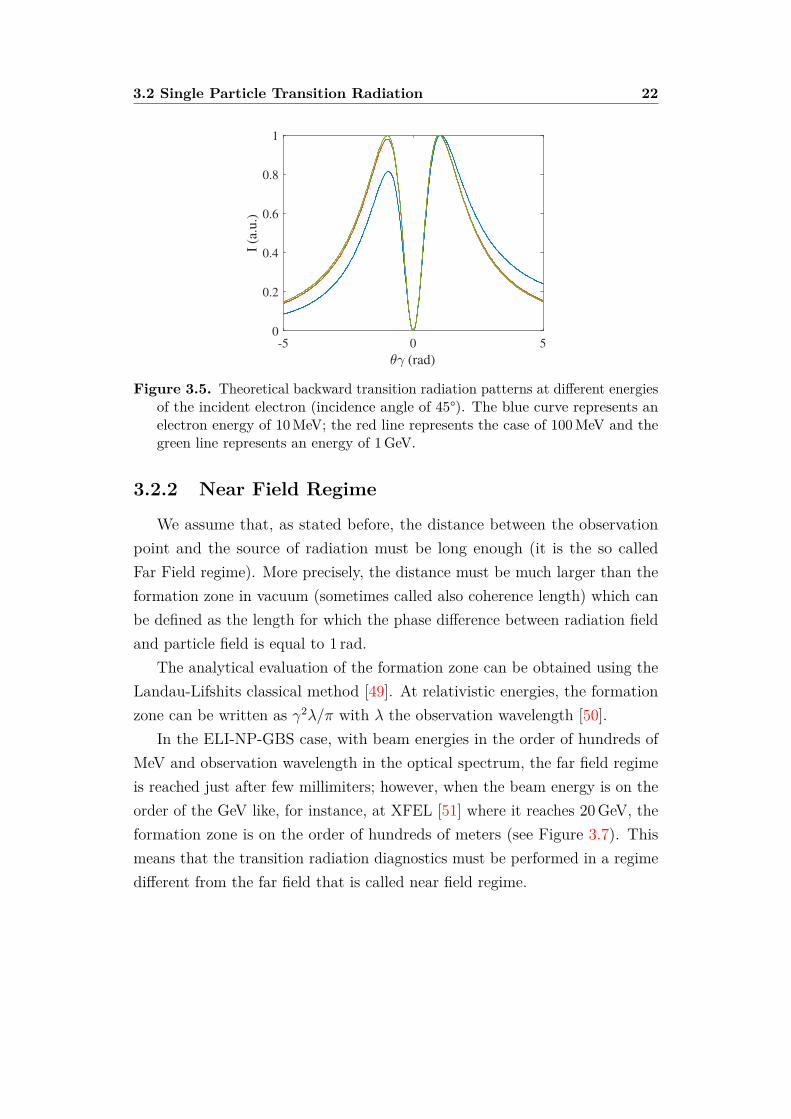
Figure 3.6. Geometry for a transition radiation screen of radius a and an observa-tion screen placed at a distance D. Picture taken from [52].
In this regime the angular distribution can be written as in Equation 3.8:[dI2
SP
dλdΩ
]Near
= e2k4
4π3ε0cβ4γ2
∣∣∣∣∣∫ a
0K1
(kρ
βγ
)J1(kρ sin θ) exp
(kρ2
2R
)ρdρ
∣∣∣∣∣2
,
(3.8)where k = 2π/λ, a is the screen transverse dimension, ρ is the radial coordinateof the source field and R is the distance from the source field [52] (see Figure 3.6).If the distance R is big enough, then the phase term in the integrand tend tounity and, assuming the transverse dimension of the screen a large enough,Equation 3.8 becomes the one of the far field regime already seen in Equation 3.5.
0 5 10 15 20
(rad)
0
0.2
0.4
0.6
0.8
1
I (a
.u.)
D=12.19m
D=121.9m
D=1219m
Figure 3.7. Near field optical transition radiation calculated according to Equa-tion 3.8: the energy is 20 GeV (the maximum energy of XFEL) and the observa-tion wavelength is 500 nm. Three different distance where considered: 12.19 m,121.9 m and 1219 m.
3.2 Single Particle Transition Radiation 24
3.2.3 Transition Radiation from Finite Screens
Another important assumption we made is that the transition radiationscreen must be infinite: under this condition the radiation can be considereda “white spectrum” (neglecting the frequency dependence of the materialreflectivity); in a more realistic condition, the transverse dimension of thescreen must be much bigger than the radial dimension of the particle field;otherwise, the fringe effects must be taken into account and the result is nolonger frequency independent. The transverse radius of the particle field isequal to γλ/2π: hence, at a fixed wavelength λ, the transverse dimension ofthe particle field is directly proportional to the energy and, at fixed energy, itis proportional to the wavelength.
Typically, for diagnostic purpose, the transition radiation is observed inthe optical spectrum (OTR): considering the maximum energy expected atELI-NP-GBS (720 MeV), the transverse dimension is about 0.2 mm while theOTR screen transverse size is 3 cm. In order to have a transverse dimensionof 3 cm at a wavelength of 700 nm, instead, the energy must be 138 GeV; forhigher energies, the fringe effects must be considered.
We now consider the effect of a finite screen on the radiation. For acylindrical geometry (see Figure 3.6), it is possible to perform this analysiswith the so called virtual photon method [52]: at the transition from vacuumto the surface (here assumed a perfectly conducting metal), virtual photons areconverted into real photons and reflected at the interface. With this approach,
0 5 10 15 20 25 30 35
(mrad)
-0.2
-0.1
0
0.1
0.2
0.3
0.4
0.5
T(
,)
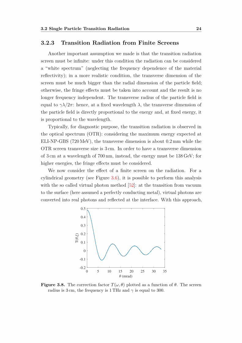
Figure 3.8. The correction factor T (ω, θ) plotted as a function of θ. The screenradius is 3 cm, the frequency is 1 THz and γ is equal to 300.

3.3 Transition Radiation from a Beam 25
a generalized Ginzburg-Frank equation can be written as:
dI2SP
dΩdλ =[dI2
SP
dΩdλ
]GF
[1− T (θ, λ)]2 , (3.9)
T (θ, λ) = 2πaλγ
J0
(2πaθλ
)K1
(2πaλγ
)+J1(
2πaθλ
)K0
(2πaλγ
)γθ
, (3.10)
where the term[dI2
SP
dΩdλ
]GF
is the classical Ginzburg-Frank formula reportedin 3.5. The generalized Ginzburg-Frank formula is now frequency dependentas can be seen in Figure 3.9; the variation with the frequency is introduced bythe correction factor T (θ, λ) expressed in Equation 3.10. The correction factoris dependent on the ratio between the screen radius a and the wavelength ofobservation. It can be verified that for a→∞ the correction factor goes to zeroand Equation 3.9 turn back into the classical Ginzburg-Frank formula; whileif a → 0, then the correction factor goes to 1 and no radiation is generated.An example of a plot of the correction factor is showed in Figure 3.8 for afrequency of 1 THz a screen radius of 3 cm and an energy of about 150 MeV.
0 2 4 6 8 10
(rad)
0
0.2
0.4
0.6
0.8
1
I (a
.u.)
Figure 3.9. Transition Radiation curve according to Equation 3.9 for a γ equalto 100 and two different frequency: a 1 THz radiation in the blue line and a560 THz radiation (green light) in the red line.
3.3 Transition Radiation from a Beam
In the previous sections, only the radiation produced by a single electronwas considered; however, in a real measurement, a complete beam with its

3.3 Transition Radiation from a Beam 26
6D distribution (transverse and longitudinal phase-space) must be taken intoaccount. The total spectral angular intensity can be written as:
dI2tot
dλdΩ = dI2SP
dλdΩ
N +N(N − 1)
∣∣∣∣∫ ∫n(ρ, z) exp
[2πλ
(z + ρ sin θ)]dρdz
∣∣∣∣2,
(3.11)where ρ and z are respectively the radial and the longitudinal positions of theN particles of the beam; dI2
SP
dλdΩ is the Single Particle Function and it is equal tothe Ginzburg-Frank formula of Equation 3.5 since we are assuming a normalincidence in a perfectly conducting metal. The function n(ρ, z) represents thecharges distribution normalized to unity [53]. The first addendum representsthe incoherent radiation and it is linearly dependent on the beam charge;the second addendum is the coherent radiation that grows quadratically withthe charge. However, in the optical spectrum with a beam with longitudinaldimension σz of mm, the integral (called form factor) tend to zero and onlythe incoherent radiation can be taken into consideration: this is related to theratio between the beam length and the wavelength.
-20 -10 0 10 20
(mrad)
0
1
2
3
4
5
6
I (a
.u.)
104
Figure 3.10. Transition Radiation for a 234 MeV energy and two different valuesof divergence: 0.1 mrad in the blue line and a 1 mrad in the red line.
In the case of beam, with energy spread and divergence, the first addendumof Equation 3.11 must be rewritten as a summation:
dI2tot
dλdΩ ∝N∑i=1
(θ − σ′i)2
1γ2
i+ (θ − σ′i)2 (3.12)
3.3 Transition Radiation from a Beam 27
where σ′ is the particle transverse momentum. The effect of the energy spreadis very weak and becomes appreciable only with values of tens of percents.Hence, neglecting the energy spread, Equation 3.12 becomes the convolutionof the single particle function with the beam divergence distribution. If wecan assume a Gaussian distribution of the divergences, the OTR angulardistribution can be written as:
I = e2
4π3cε0
√πµ
ν<[Φ(z)
(12 + µνz
)]− µ2,
µ = 1√2σ′
, Φ(z) = 1− erf (z)exp [−z2] ,
z = µ(ν + iθ), ν = 1γ, (3.13)
where erf(z) is the complex error function and < is the real part [54]. Assuminga Gaussian distribution of the particle transverse momentum is reasonablein most of the cases; however, where there are strong correlations betweenposition and angle, or between horizontal and vertical planes, or in generalwhen the distribution is not anymore Gaussian this treatment cannot be applyand a reasonable guess of such a distribution must be considered.
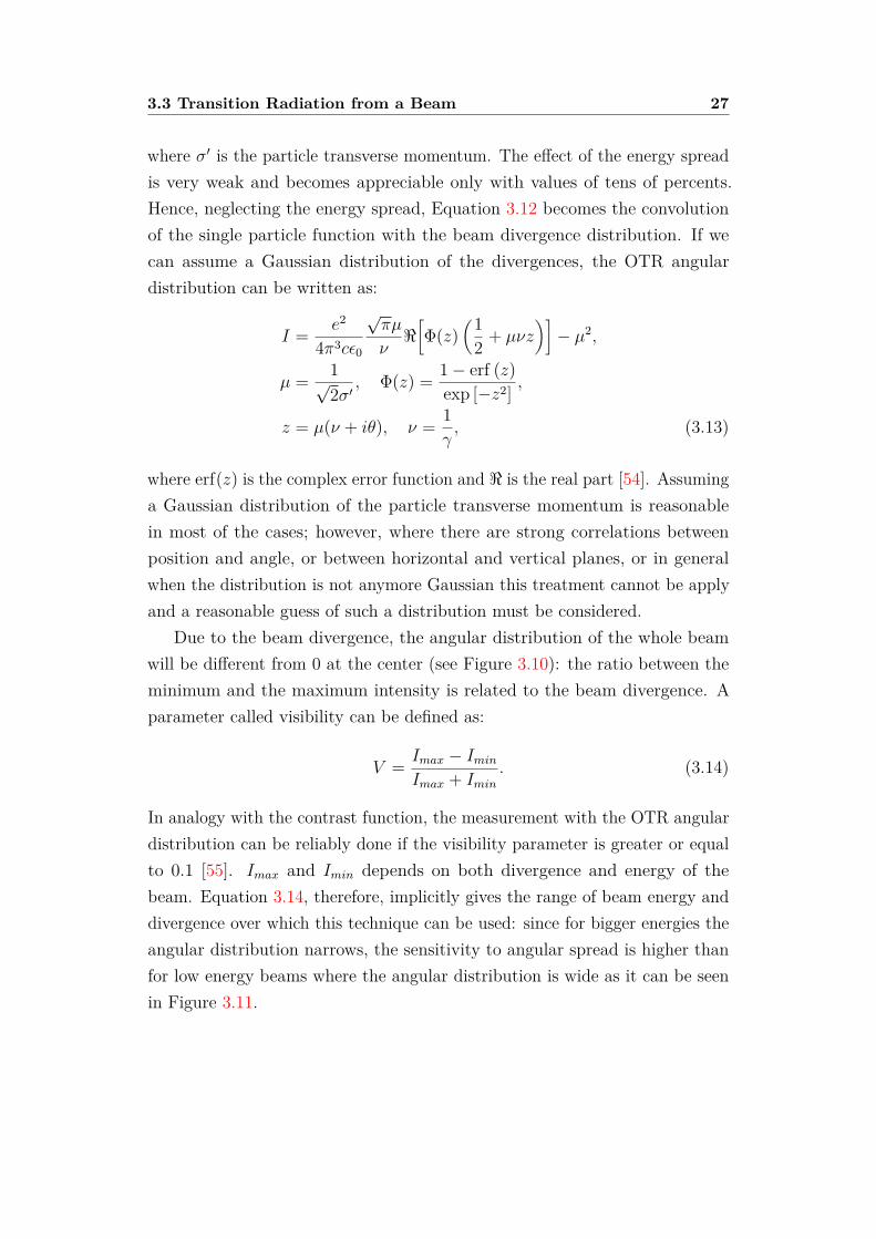
Due to the beam divergence, the angular distribution of the whole beamwill be different from 0 at the center (see Figure 3.10): the ratio between theminimum and the maximum intensity is related to the beam divergence. Aparameter called visibility can be defined as:
V = Imax − IminImax + Imin
. (3.14)
In analogy with the contrast function, the measurement with the OTR angulardistribution can be reliably done if the visibility parameter is greater or equalto 0.1 [55]. Imax and Imin depends on both divergence and energy of thebeam. Equation 3.14, therefore, implicitly gives the range of beam energy anddivergence over which this technique can be used: since for bigger energies theangular distribution narrows, the sensitivity to angular spread is higher thanfor low energy beams where the angular distribution is wide as it can be seenin Figure 3.11.
3.3 Transition Radiation from a Beam 28
0 500 1000 1500 2000 2500 30000
2
4
6
8
10
(m
rad)
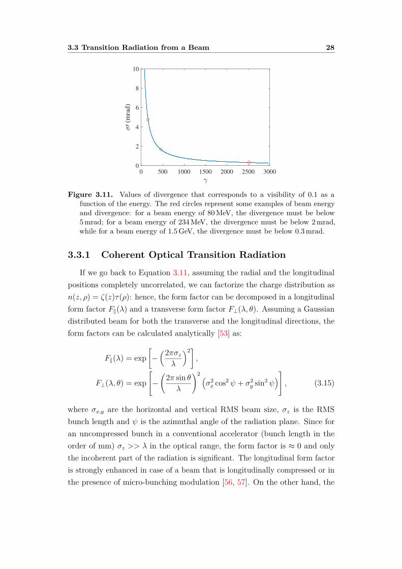
Figure 3.11. Values of divergence that corresponds to a visibility of 0.1 as afunction of the energy. The red circles represent some examples of beam energyand divergence: for a beam energy of 80 MeV, the divergence must be below5 mrad; for a beam energy of 234 MeV, the divergence must be below 2 mrad,while for a beam energy of 1.5 GeV, the divergence must be below 0.3 mrad.
3.3.1 Coherent Optical Transition Radiation
If we go back to Equation 3.11, assuming the radial and the longitudinalpositions completely uncorrelated, we can factorize the charge distribution asn(z, ρ) = ζ(z)τ(ρ): hence, the form factor can be decomposed in a longitudinalform factor F‖(λ) and a transverse form factor F⊥(λ, θ). Assuming a Gaussiandistributed beam for both the transverse and the longitudinal directions, theform factors can be calculated analytically [53] as:
F‖(λ) = exp[−(2πσz
λ
)2],
F⊥(λ, θ) = exp−(2π sin θ
λ
)2 (σ2x cos2 ψ + σ2
y sin2 ψ) , (3.15)
where σx,y are the horizontal and vertical RMS beam size, σz is the RMSbunch length and ψ is the azimuthal angle of the radiation plane. Since foran uncompressed bunch in a conventional accelerator (bunch length in theorder of mm) σz >> λ in the optical range, the form factor is ≈ 0 and onlythe incoherent part of the radiation is significant. The longitudinal form factoris strongly enhanced in case of a beam that is longitudinally compressed or inthe presence of micro-bunching modulation [56, 57]. On the other hand, the
3.3 Transition Radiation from a Beam 29
transverse form factor is responsible of an angular distribution narrower andless intense as the transverse beam size increase.
Due to the quadratic dependence with the charge, coherent radiation coulddisturb or even mask completely the measurement of the incoherent angulardistribution; some authors [58] propose to image the beam in the ultravioletspectrum to avoid the coherence radiation disturbs. On the other hand,the coherent radiation has been used as a tool to retrieve the longitudinalinformation of the beam [59] or as a source of THz radiation [60].
30
Chapter 4
Design Issue
As it was shown in the Chapter 3, the Transition Radiation happens whena charged particle crosses the boundary between two media with differentelectrical properties (i.e. different dielectric constant). However, depending onits charge, the particle beam may deposit not negligible amounts of energy inthe target material due to this interaction. This phenomenon could determine atemperature increase that may deform the OTR target surface; this deformationmay influence the photon emission and the diagnostics quality.
This chapter presents a study on the thermal behavior of the OTR screen(Section 4.1), using as target material aluminum and silicon [1, 61].
Similar studies have been done at the CLIC Test Facility [62], at TTF2 [63],at ATF [64] and at CEBAF [65]. Many authors propose, in case of highcharge and high repetition rate, the use of graphite target (CLIC), carbon foil(CEBAF) or Beryllium target (ATF): however, in the ELI-NP-GBS case, theresolution needed imposes a planarity requirement of the screen surface thatthose materials do not fit. At LCLS-II [66], instead, they will use only wirescanner for the high quality transverse diagnostic, and the OTR screen willbe used only in the low repetition rate diagnostic line (120 Hz while the mainbeam line work at 1 MHz). Table 4.1 summarizes the main beam parametersof the above mentioned machine. However, it will be shown that the thermalstress induced by the ELI-NP-GBS beam is not as high as for the CLIC andATF case, hence a silicon screen is a good candidate.
This study has been validated by a numerical study with ANSYS simulation(Section 4.2); ANSYS was also used for the evaluation of the mean lifetimeof the studied materials and to evaluate the shape and the amplitude of the
4.1 Thermal Analysis 31
Table 4.1. Beam parameters for different machines.
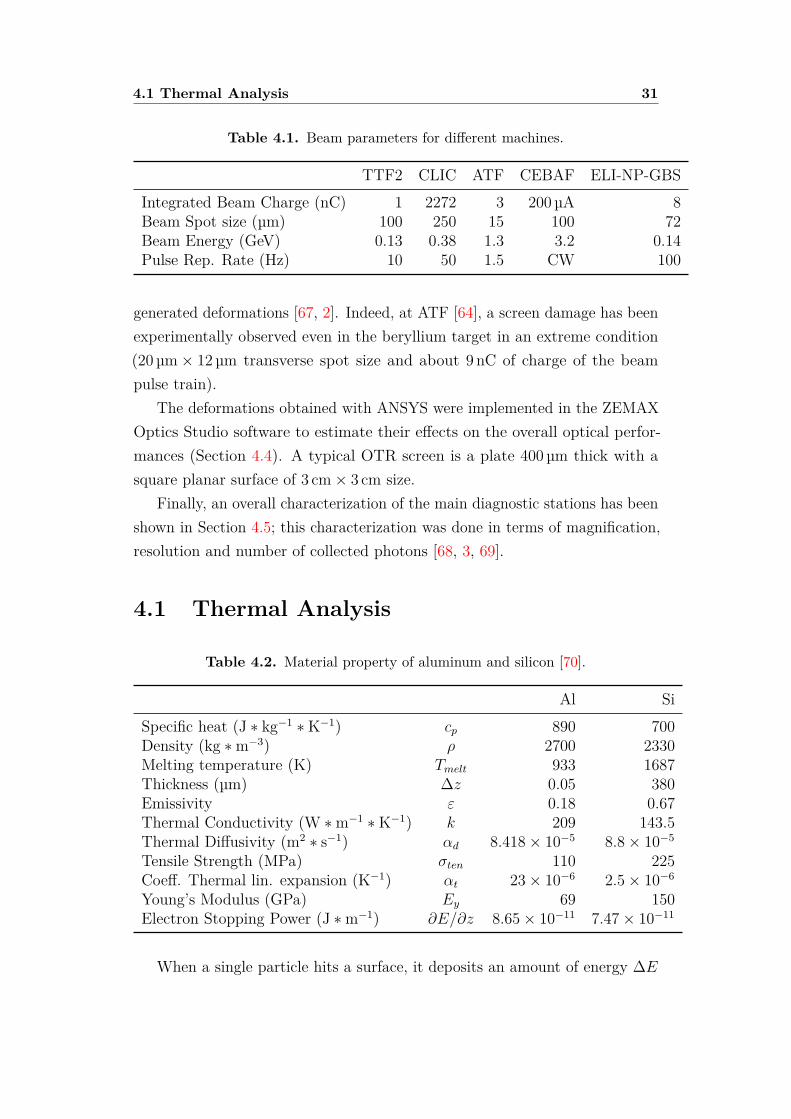
TTF2 CLIC ATF CEBAF ELI-NP-GBSIntegrated Beam Charge (nC) 1 2272 3 200 µA 8Beam Spot size (µm) 100 250 15 100 72Beam Energy (GeV) 0.13 0.38 1.3 3.2 0.14Pulse Rep. Rate (Hz) 10 50 1.5 CW 100
generated deformations [67, 2]. Indeed, at ATF [64], a screen damage has beenexperimentally observed even in the beryllium target in an extreme condition(20 µm× 12 µm transverse spot size and about 9 nC of charge of the beampulse train).
The deformations obtained with ANSYS were implemented in the ZEMAXOptics Studio software to estimate their effects on the overall optical perfor-mances (Section 4.4). A typical OTR screen is a plate 400 µm thick with asquare planar surface of 3 cm× 3 cm size.
Finally, an overall characterization of the main diagnostic stations has beenshown in Section 4.5; this characterization was done in terms of magnification,resolution and number of collected photons [68, 3, 69].
4.1 Thermal Analysis
Table 4.2. Material property of aluminum and silicon [70].
Al SiSpecific heat (J ∗ kg−1 ∗K−1) cp 890 700Density (kg ∗m−3) ρ 2700 2330Melting temperature (K) Tmelt 933 1687Thickness (µm) ∆z 0.05 380Emissivity ε 0.18 0.67Thermal Conductivity (W ∗m−1 ∗K−1) k 209 143.5Thermal Diffusivity (m2 ∗ s−1) αd 8.418× 10⁻⁵ 8.8× 10⁻⁵
Tensile Strength (MPa) σten 110 225Coeff. Thermal lin. expansion (K−1) αt 23× 10−6 2.5× 10⁻⁶
Young’s Modulus (GPa) Ey 69 150Electron Stopping Power (J ∗m−1) ∂E/∂z 8.65× 10⁻¹¹ 7.47× 10⁻¹¹
When a single particle hits a surface, it deposits an amount of energy ∆E
4.1 Thermal Analysis 32
according to:∆E = ∂E
∂zρ∆z, (4.1)
where ρ is the density of the material and ∆z is its thickness; the electron stop-ping power ∂E/∂z depends on the material and on the particle energy while,here, it can be considered spatially independent. Often, in literature, the massstopping power, which is obtained by dividing the electron stopping power bythe density material, is instead used: in this way, the value is material indepen-dent. Typical values used for the energy of interest are 2 MeV ∗ cm2 ∗ g−1 [62]or 1.61 MeV ∗ cm2 ∗ g−1 [63] or 1.64 MeV ∗ cm2 ∗ g−1 [71]; For all the calcula-tion showed in this work, the values in Table 4.2 has been used: this gives amass stopping power of 2 MeV ∗ cm2 ∗ g−1.
Assuming an electron beam with a Gaussian spatial distribution hittingthe surface, the target temperature T (x, y, t) obeys to the equation [72]:
∂T (x, y, t)∂t
= 1cpρ
∂E
∂z
Ne(t)ρ2πσxσy
exp(− x2
2σ2x
− y2
2σ2y
)+
k∇2T (x, y, t)− 2εσsb∆z
[T (x, y, t)4 − T 4
0
], (4.2)
where x and y are the transverse position of the beam, σx (σy) represents thetransverse beam size, cp is the specific heat, Ne(t) is the number of particleof the beam, k is the thermal conductivity, ε is the emissivity and σsb is theStephan-Boltzmann constant. The first addendum represents the temperaturerising, the second one is the cooling by conduction and the third one is theradiation cooling, while, since the target is in vacuum, there is not convectioncooling.
When a bunch hits the screen, the temperature rises according to [62]:
T (x, y)− T0 = ∂E
∂z
Ne
2πσxσycpexp
(− x2
2σ2x
− y2
2σ2y
). (4.3)
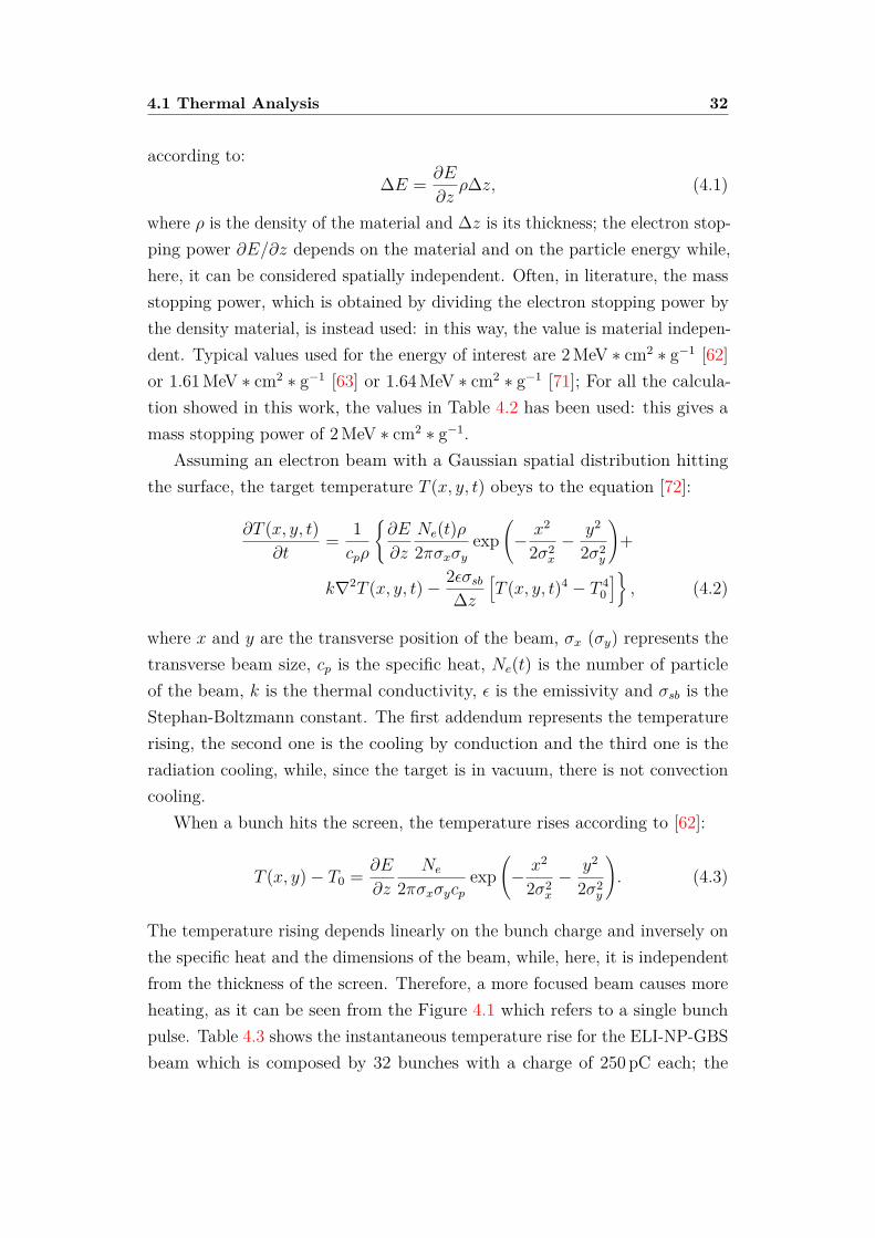
The temperature rising depends linearly on the bunch charge and inversely onthe specific heat and the dimensions of the beam, while, here, it is independentfrom the thickness of the screen. Therefore, a more focused beam causes moreheating, as it can be seen from the Figure 4.1 which refers to a single bunchpulse. Table 4.3 shows the instantaneous temperature rise for the ELI-NP-GBSbeam which is composed by 32 bunches with a charge of 250 pC each; the
4.1 Thermal Analysis 33
50 100 150 200 250 300
x
y ( m)
10-1
100
101
T+ (
K)
Al
Si
(a)
50 100 150 200 250 300
x
y ( m)
10-2
100
T+ (
K)
20 pC
250 pC
400 pC
(b)
Figure 4.1. Instantaneous temperature rising as a function of the beam dimensionsfor two different material (aluminum and silicon) and a bunch charge of 250 pC(a). Figure (b) represents the case of an aluminum screen and three differentbunch charges (20 pC, 250 pC and 400 pC). The triangles represent the valuesat the position of the OTR diagnostic stations in the ELI-NP-GBS Linac (seeTable 4.3).
spot sizes are the one estimated by beam dynamic simulations at the OTRdiagnostic stations. When the beam spot size is 47.5 µm× 109 µm (the beamwith higher charge density), the temperature increase is higher: therefore, thiscase will be studied in more details.
Table 4.3. Instantaneous temperature increase for a 32 bunches train with a chargeof 250 pC each at the position of the OTR diagnostic stations in the ELI-NP-GBSLinac. The beam with the higher charge density has been emphasized in boldcharacter: it causes the higher temperature increase, hence it will be studied inmore details.
σx(σy)(µm) ∆T+ Al (K) ∆T+ Si (K)298 (298) 3 4251 (252) 5 6211 (213) 6 8184 (184) 8 1147.5 (109) 55 70241 (27.4) 43 55106 (70) 39 49
For the ELI-NP-GBS case, the temperature increase stays well below fewhundreds of Kelvin: hence, the radiative cooling can be considered negligiblesince it becomes relevant for temperature above 1000 K. Therefore, it must betaken into account only the conduction cooling. Typically, “cooling mechanism”
4.1 Thermal Analysis 34
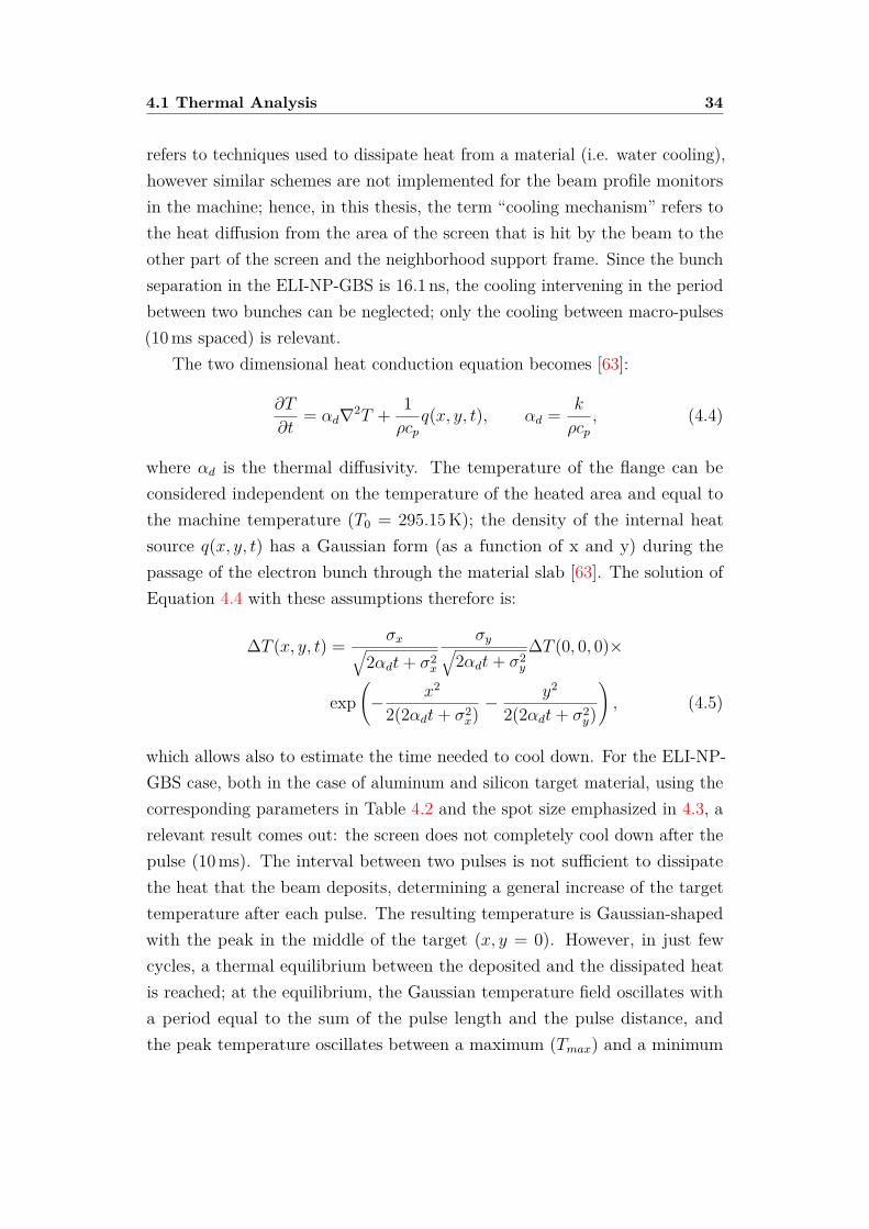
refers to techniques used to dissipate heat from a material (i.e. water cooling),however similar schemes are not implemented for the beam profile monitorsin the machine; hence, in this thesis, the term “cooling mechanism” refers tothe heat diffusion from the area of the screen that is hit by the beam to theother part of the screen and the neighborhood support frame. Since the bunchseparation in the ELI-NP-GBS is 16.1 ns, the cooling intervening in the periodbetween two bunches can be neglected; only the cooling between macro-pulses(10 ms spaced) is relevant.
The two dimensional heat conduction equation becomes [63]:
∂T
∂t= αd∇2T + 1
ρcpq(x, y, t), αd = k
ρcp, (4.4)
where αd is the thermal diffusivity. The temperature of the flange can beconsidered independent on the temperature of the heated area and equal tothe machine temperature (T0 = 295.15 K); the density of the internal heatsource q(x, y, t) has a Gaussian form (as a function of x and y) during thepassage of the electron bunch through the material slab [63]. The solution ofEquation 4.4 with these assumptions therefore is:
∆T (x, y, t) = σx√2αdt+ σ2
x
σy√2αdt+ σ2
y
∆T (0, 0, 0)×
exp(− x2
2(2αdt+ σ2x)− y2
2(2αdt+ σ2y)
), (4.5)
which allows also to estimate the time needed to cool down. For the ELI-NP-GBS case, both in the case of aluminum and silicon target material, using thecorresponding parameters in Table 4.2 and the spot size emphasized in 4.3, arelevant result comes out: the screen does not completely cool down after thepulse (10 ms). The interval between two pulses is not sufficient to dissipatethe heat that the beam deposits, determining a general increase of the targettemperature after each pulse. The resulting temperature is Gaussian-shapedwith the peak in the middle of the target (x, y = 0). However, in just fewcycles, a thermal equilibrium between the deposited and the dissipated heatis reached; at the equilibrium, the Gaussian temperature field oscillates witha period equal to the sum of the pulse length and the pulse distance, andthe peak temperature oscillates between a maximum (Tmax) and a minimum

4.1 Thermal Analysis 35
0.1 0.2 0.3 0.4 0.5
t (ms)
290
300
310
320
330
340
350
360
370
T (
K)
Al
Si
Figure 4.2. Temporal evolution of the conduction cooling after the heating of aELI-NP-GBS bunch train (σx =47.5 µm, σy =109 µm). The values refer to thecenter of the impact area of the beam to the target (x, y = 0).
(Tmin) value (“steady-state oscillation”). Figure 4.2 and Figure 4.3 show thatafter three cycles, an equilibrium is reached: the minimum temperatures are295.3 K for the aluminum and 295.4 K for the silicon, while the maximum onesare 350.6 K for the aluminum and 365.8 K for the silicon.
5 10 15 20 25 30 35 40 45
t (ms)
290
300
310
320
330
340
350
360
T (
K)
Figure 4.3. Temporal evolution of the heated area during 4 cycles of ELI-NP-GBSmachine operation with a bunch train of σx =47.5 µm and σy =109 µm. Thevalues refer to the center of the impact area of the beam to the aluminum target(x, y = 0).
4.2 ANSYS Numerical Analysis 36
4.2 ANSYS Numerical Analysis
As explained in Section 4.3, the impact of the electron beam on theOTR screen, produces a continuous oscillating change of temperature of thematerial. The theoretical approach suggests that the oscillations reach anequilibrium condition after few cycles. The thermal simulation has beenperformed in ANSYS environment to validate the theory and to assess thetemperature distribution over the time. Several thermal transient analysis hasbeen performed with a dedicate ANSYS analysis.
The study of localized heating and of the cooling of the OTR target(“thermal cycle”) requires the simulation of high number of impacts of theelectrons. In light of this, the energy deposited by the beam is provided tothe 3D mesh elements corresponding to the OTR target portion significantlyinteracting with the electron beam (“hotspot”).
A non uniform mesh was used and it was refined close to the hotspot wherethe heat generation is concentrated (minimum mesh size of 6 µm). Regardingthe boundary condition, it was considered an initial temperature T0 of 295.15 K,corresponding to the ELI-NP-GBS machine temperature. This temperaturewas fixed along the edges in contact with the frame support and the screws.
The analysis introduces an approximation for the simulation of the depositedenergy distribution: indeed, it associates to each entire mesh element a valuecalculated with the coordinates of its centroid and the electron beam properties.However, a comparison between data obtained with the analytical formulaand those extracted from ANSYS simulations confirms the goodness of theapproximation.
Results of the thermal transient analysis are reported in Figure 4.4. Itwas also used a uniform thermal power distribution: in this case, the scriptassociates to all the nodes within the elliptic beam section the temperaturegiven by Equation 4.3 for x = y = 0 (350 K), and the machine temperatureto the remaining nodes). Silicon presents a much more pronounced increaseof temperature in the interaction area, with respect to the aluminum: this isa reasonable result taking into account the higher specific heat capacity anddensity of the aluminum with respect to the silicon for the same depositedelectron beam energy. Aluminum reaches a steady-state maximum peaktemperature of 345.3 K after about 80 thermal cycles, while silicon reaches
4.3 Thermal Stress Evaluation 37
0.2 0.4 0.6 0.8 1
t (ms)
290
300
310
320
330
340
T (
K)
Theory (Gaussian Distr.)
ANSYS (Gaussian Distr.)
ANSYS (Uniform Distr.)
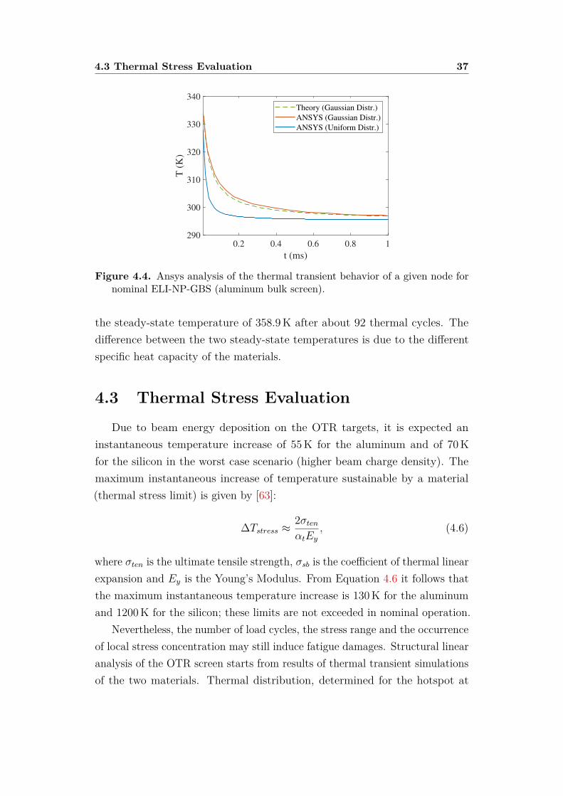
Figure 4.4. Ansys analysis of the thermal transient behavior of a given node fornominal ELI-NP-GBS (aluminum bulk screen).
the steady-state temperature of 358.9 K after about 92 thermal cycles. Thedifference between the two steady-state temperatures is due to the differentspecific heat capacity of the materials.
4.3 Thermal Stress Evaluation
Due to beam energy deposition on the OTR targets, it is expected aninstantaneous temperature increase of 55 K for the aluminum and of 70 Kfor the silicon in the worst case scenario (higher beam charge density). Themaximum instantaneous increase of temperature sustainable by a material(thermal stress limit) is given by [63]:
∆Tstress ≈2σtenαtEy
, (4.6)
where σten is the ultimate tensile strength, σsb is the coefficient of thermal linearexpansion and Ey is the Young’s Modulus. From Equation 4.6 it follows thatthe maximum instantaneous temperature increase is 130 K for the aluminumand 1200 K for the silicon; these limits are not exceeded in nominal operation.
Nevertheless, the number of load cycles, the stress range and the occurrenceof local stress concentration may still induce fatigue damages. Structural linearanalysis of the OTR screen starts from results of thermal transient simulationsof the two materials. Thermal distribution, determined for the hotspot at
4.3 Thermal Stress Evaluation 38
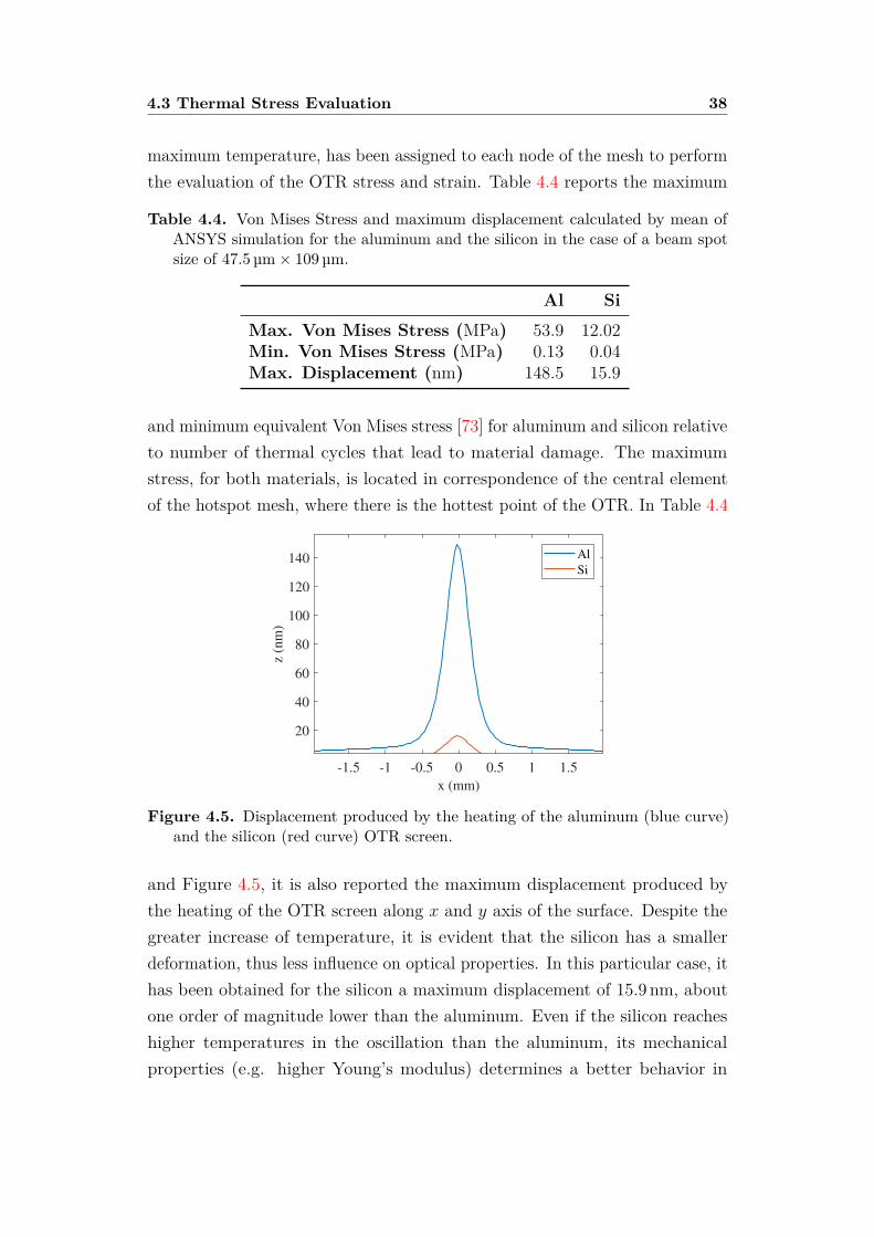
maximum temperature, has been assigned to each node of the mesh to performthe evaluation of the OTR stress and strain. Table 4.4 reports the maximum
Table 4.4. Von Mises Stress and maximum displacement calculated by mean ofANSYS simulation for the aluminum and the silicon in the case of a beam spotsize of 47.5 µm× 109 µm.
Al SiMax. Von Mises Stress (MPa) 53.9 12.02Min. Von Mises Stress (MPa) 0.13 0.04Max. Displacement (nm) 148.5 15.9
and minimum equivalent Von Mises stress [73] for aluminum and silicon relativeto number of thermal cycles that lead to material damage. The maximumstress, for both materials, is located in correspondence of the central elementof the hotspot mesh, where there is the hottest point of the OTR. In Table 4.4
-1.5 -1 -0.5 0 0.5 1 1.5
x (mm)
20
40
60
80
100
120
140
z (
nm
)
Al
Si
Figure 4.5. Displacement produced by the heating of the aluminum (blue curve)and the silicon (red curve) OTR screen.
and Figure 4.5, it is also reported the maximum displacement produced bythe heating of the OTR screen along x and y axis of the surface. Despite thegreater increase of temperature, it is evident that the silicon has a smallerdeformation, thus less influence on optical properties. In this particular case, ithas been obtained for the silicon a maximum displacement of 15.9 nm, aboutone order of magnitude lower than the aluminum. Even if the silicon reacheshigher temperatures in the oscillation than the aluminum, its mechanicalproperties (e.g. higher Young’s modulus) determines a better behavior in
4.3 Thermal Stress Evaluation 39
terms of deformation that reflects in better optical quality of the screen and,thus, of the whole diagnostic system.
The equivalent Von Mises stress (σVM ), obtained in the structural analysis(Table 4.4), has been used to estimate alternating (σa) and mean (σm) stressintensity:
σa = σVMmax − σVMmin
2 ,
σm = σVMmax + σVMmin
2 . (4.7)
Consequently, to quantify the interaction of mean and alternating stresses, ithas been applied the Goodman relation:
σaσN
+ σmσten
= 1, (4.8)
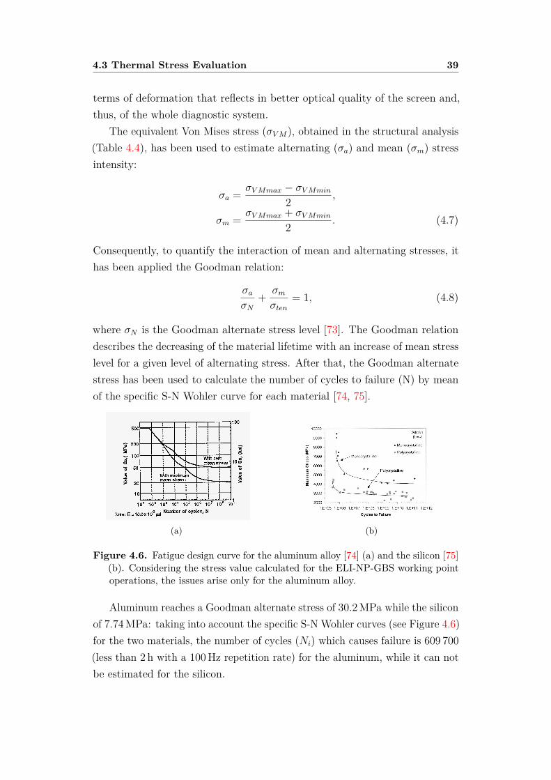
where σN is the Goodman alternate stress level [73]. The Goodman relationdescribes the decreasing of the material lifetime with an increase of mean stresslevel for a given level of alternating stress. After that, the Goodman alternatestress has been used to calculate the number of cycles to failure (N) by meanof the specific S-N Wohler curve for each material [74, 75].
(a) (b)
Figure 4.6. Fatigue design curve for the aluminum alloy [74] (a) and the silicon [75](b). Considering the stress value calculated for the ELI-NP-GBS working pointoperations, the issues arise only for the aluminum alloy.
Aluminum reaches a Goodman alternate stress of 30.2 MPa while the siliconof 7.74 MPa: taking into account the specific S-N Wohler curves (see Figure 4.6)for the two materials, the number of cycles (Ni) which causes failure is 609 700(less than 2 h with a 100 Hz repetition rate) for the aluminum, while it can notbe estimated for the silicon.
4.4 Optical System Simulation 40
Table 4.5. Effects of the multibunching on the thermal and the mechanicalparameter of the aluminum.
# Bunches Max. Temp. (K) σa (MPa) MTBF (h)32 344.4 30.2 < 216 320.2 13.93 ∞8 307.7 6.99 ∞
On the other hand, changing the characteristics of electron beam, i.e.decreasing the number of bunches, the fatigue life for aluminum increases: therising of maximum temperature and thus mechanical stresses, are inverselyproportional to the bunches’ number (Table 4.5). For example, with 16 bunchesinstead of 32, also aluminum has no fatigue life limit just like silicon.
4.4 Optical System Simulation
A high distortion of the OTR screen surface close to the electron beamhotspot could generate a loss of image resolution [64]. For a generic monocrys-talline silicon plate, the production mean square roughness is under 1 nm;therefore, the evaluation of the OTR screen strain surface is relevant for itsoptical performance. The prediction of the optical performances is typicallydone with commercially available optical design software such as ZEMAX [76]or CODEV; these softwares allow to represent surface errors and displacementsby means of polynomial surface definition, surface interferogram files or uniformarray of data.
The surface errors are defined by means of surface normal or sag displace-ment: the sag displacement is defined as the distance from the vertex tangentplane to the optical surface. ZEMAX implements the data array with the socalled “Grid Sag Surface”: it is a uniform array of sag displacement and/orslope data used to define a perturbation to a base surface (in our case a planarsurface).
ZEMAX offers different ways to evaluate the performances of an opticsystem: the main ones are the geometric RMS spot size diameter and thePhysical Optic Propagation Mode (POP). In the first case, a simple geometricalray tracing analysis is performed assuming an object at infinity and threedifferent wavelengths (486 nm, 588 nm, 656 nm): this method, however, is not

4.4 Optical System Simulation 41
reliable in some application like, for instance, when the system is close to thediffraction limit. A more precise analysis can be done with the POP modewhich take into account also diffraction and polarization of light.
The photons are reflected by a deformed mirror and then they are collectedby an optical system to perform the imaging of the source. A Gaussianbeam with the same spot size as the electron beam under study (see the boldline in Table 4.3) has been propagated through the optic system; the mirrordeformation has been defined in accordance with the displacement created bythe beam on the aluminum target and on the silicon target (149 nm and 16 nmrespectively, as can be seen in Table 4.4).
-500 0 500
u ( m)
0
0.2
0.4
0.6
0.8
1
I (a
.u.)
y undeformed
y Al
y Si
Figure 4.7. Vertical profile of a beam reflected by a mirror in the perfectly planarcase (blue continuous line) and in the case of an aluminum deformation (redcontinuous line) and a silicon deformation (green dashed line).
The deformation causes a small translation of the centroids of the beam(below 1.4 µm for the silicon case and below 10 µm for the aluminum case); italso causes a loss of the collected photons which is negligible for the silicon case(0.4%) while it goes up to 30% for the aluminum case. A bigger issue is relatedto the Gaussian reconstruction of the beam in the case of the aluminum: it isnegligible for the horizontal plane (47.5 µm) while is 44% in the vertical plane(109 µm), as can be seen in Figure 4.7.
This dependence of the error on the spot size is confirmed also by othersimulations for different beam size: for instance, a 27 µm symmetric beam getdeformed by a factor lesser than 0.01. Also the centroids and the amplitudeare less affected by the displacement; furthermore, the effect is more significanton the vertical plane, where the deformation of the screen is larger. The reason

4.5 Resolution 42
is related to the area of displacement where the beam is reflected: a biggerbeam is reflected by a larger area of the deformed mirror. Indeed, the largerbeam “sees” a bigger portion of the displacement.
These results show that the optical properties of the silicon screen do notchange significantly even after the thermal deformation, while the ones of thealuminum screen are heavily compromised. As a result of these studies, asilicon OTR screen has been chosen for the diagnostic station; furthermore,in order to reduce the loss of optical performance and to obtain an easierlithography process of the OTR surface for the image calibration (as it will beexplain next), the silicon used to produce the electrical chip has been chosen(monochristalline silicon wafer): the main characteristic is indeed the goodplanarity of the surface.
4.5 Resolution
The expected RMS beam size along the LINAC, provided by preliminarybeam dynamics simulation, will vary in the 30 µm - 1000 µm range [77] (asreported in Figure 4.8). An evaluation has been done in order to find the bestlenses setup that fits the requirements in term of resolution and magnificationfor each diagnostic station.
0 5 10 15 20 25
Position along the linac startig at M4 module (m)
0
100
200
300
400
(m
)
x
y
x @ Screen
y @ Screen
Figure 4.8. Spot size of the beam in the low energy line after the S-band photoin-jector [77].
The optical acquisition system is constituted by the CCD camera “Baslerscout A640-70gm” with a macro lens. A movable slide is used to place the
4.5 Resolution 43
lens plus camera system closer or farer from the OTR target; such distanceis between 60 cm and 130 cm from the OTR target due to mechanical andgeometrical constraints. In order to avoid possible damage of the optics devicesdue to the radiation emitted by the beam, a 45° mirror is placed at 40 cm fromthe target leading to a minimum distance achievable of 60 cm; since the beampipe is placed 1.5 m from the floor, the maximum distance is instead 130 cm.
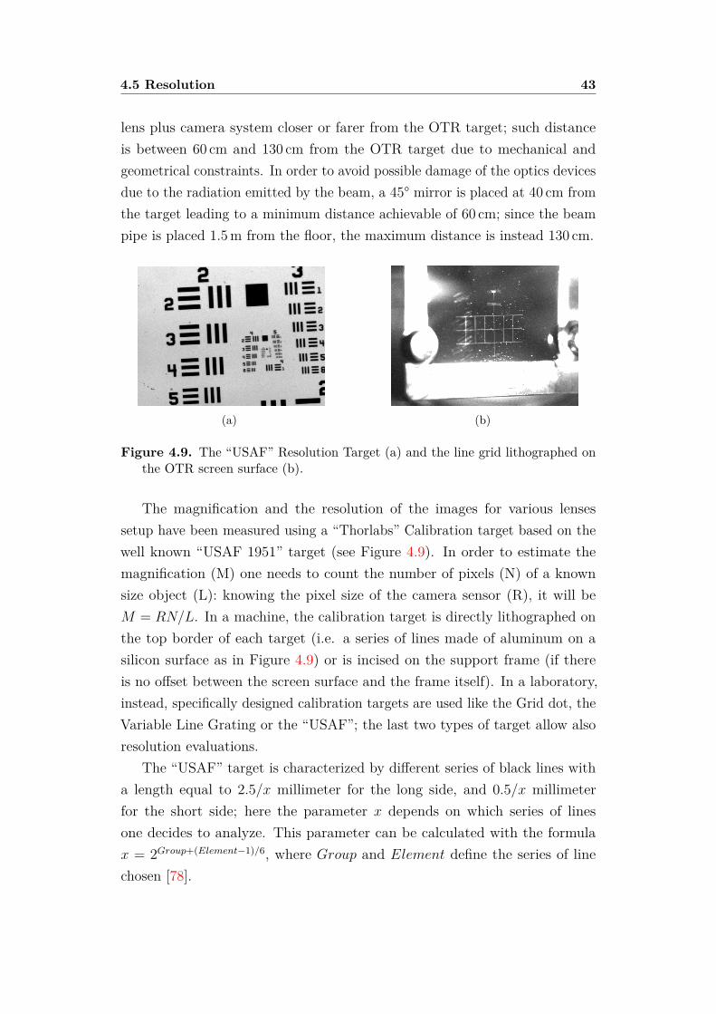
(a) (b)
Figure 4.9. The “USAF” Resolution Target (a) and the line grid lithographed onthe OTR screen surface (b).
The magnification and the resolution of the images for various lensessetup have been measured using a “Thorlabs” Calibration target based on thewell known “USAF 1951” target (see Figure 4.9). In order to estimate themagnification (M) one needs to count the number of pixels (N) of a knownsize object (L): knowing the pixel size of the camera sensor (R), it will beM = RN/L. In a machine, the calibration target is directly lithographed onthe top border of each target (i.e. a series of lines made of aluminum on asilicon surface as in Figure 4.9) or is incised on the support frame (if thereis no offset between the screen surface and the frame itself). In a laboratory,instead, specifically designed calibration targets are used like the Grid dot, theVariable Line Grating or the “USAF”; the last two types of target allow alsoresolution evaluations.
The “USAF” target is characterized by different series of black lines witha length equal to 2.5/x millimeter for the long side, and 0.5/x millimeterfor the short side; here the parameter x depends on which series of linesone decides to analyze. This parameter can be calculated with the formulax = 2Group+(Element−1)/6, where Group and Element define the series of linechosen [78].

4.5 Resolution 44
This target has been used to characterize different objectives at differentdistances in order to find the best solutions for each diagnostic station interms of magnification, resolution and field of view. Furthermore, the choiceof the more appropriate magnification (hence, of the optic system) is alsorelated to the number of photons per pixel collected, as it will be explainedin the Section 4.6. The results in terms of magnification are summarized
60 70 80 90 100 110 120 130
Distance (cm)
2
4
6
8
10
12
M-1
Figure 4.10. Inverse of the magnification as a function of the distance betweenthe target and the camera sensor for different objectives. The blue line (fit) anddot (data) represent the 105 mm; the red ones the 105 mm with teleconverter2x; the green ones the 180 mm; the black ones the 180 mm with teleconverter2x and the magenta ones the 180 mm with teleconverter 1.4x. The dashed cyanline represents the magnification required in order to image all the OTR target(3 cm), while the brown one represents the magnification needed for imaging abeam of 1 mm size (see Table 4.6).
in the Figure 4.10; it can be seen that the only lens that allows to reach amagnification equal to 1 with the above mentioned geometric constraints isthe 180 mm with a teleconverter 2x. On the other hand, the increase of thefocal length (f) limits the minimum magnification achievable in the samedistance range; hence, also the field of view is limited. Therefore, a compromisebetween maximum magnification and a higher flexibility in magnification rangeachievable needs to be done; this flexibility is useful for instance during theconditioning of the machine, when a change of the beam parameters mayrequire a fast change of the diagnostic setup. Lenses with higher focal length(i.e. 300 mm) can not be used with the current diagnostic stations due togeometric constraints.
The field of view is a parameter strictly related to the magnification; it
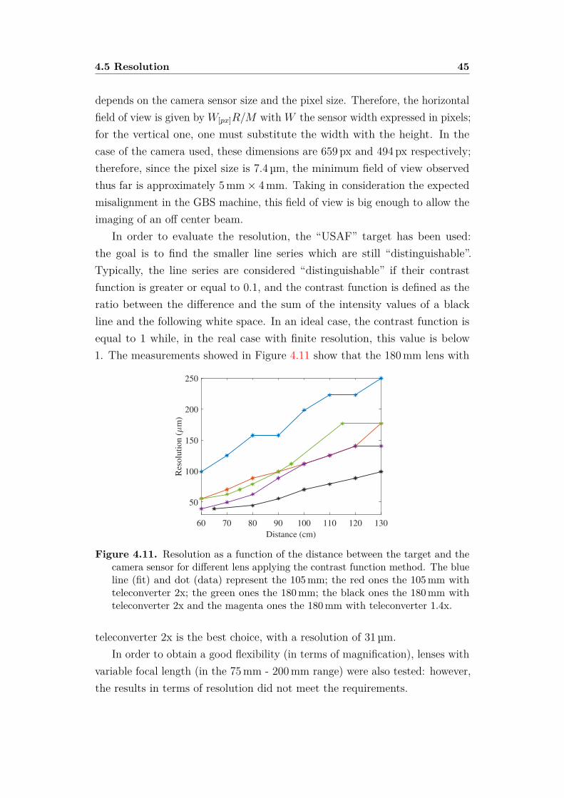
4.5 Resolution 45
depends on the camera sensor size and the pixel size. Therefore, the horizontalfield of view is given byW[px]R/M withW the sensor width expressed in pixels;for the vertical one, one must substitute the width with the height. In thecase of the camera used, these dimensions are 659 px and 494 px respectively;therefore, since the pixel size is 7.4 µm, the minimum field of view observedthus far is approximately 5 mm× 4 mm. Taking in consideration the expectedmisalignment in the GBS machine, this field of view is big enough to allow theimaging of an off center beam.
In order to evaluate the resolution, the “USAF” target has been used:the goal is to find the smaller line series which are still “distinguishable”.Typically, the line series are considered “distinguishable” if their contrastfunction is greater or equal to 0.1, and the contrast function is defined as theratio between the difference and the sum of the intensity values of a blackline and the following white space. In an ideal case, the contrast function isequal to 1 while, in the real case with finite resolution, this value is below1. The measurements showed in Figure 4.11 show that the 180 mm lens with
60 70 80 90 100 110 120 130
Distance (cm)
50
100
150
200
250
Reso
luti
on
(m
)
Figure 4.11. Resolution as a function of the distance between the target and thecamera sensor for different lens applying the contrast function method. The blueline (fit) and dot (data) represent the 105 mm; the red ones the 105 mm withteleconverter 2x; the green ones the 180 mm; the black ones the 180 mm withteleconverter 2x and the magenta ones the 180 mm with teleconverter 1.4x.
teleconverter 2x is the best choice, with a resolution of 31 µm.In order to obtain a good flexibility (in terms of magnification), lenses with
variable focal length (in the 75 mm - 200 mm range) were also tested: however,the results in terms of resolution did not meet the requirements.

4.5 Resolution 46
A camera with a different pixel size (3.75 µm instead of 7.4 µm) has beentested too; however, the overall resolution does not change too much (≈ 3%).This is because the contribution of camera sensor to the overall resolutionis small with respect to the other contribution related to the objective, lensaberrations, etc.
Another method to evaluate the resolution is based on the analysis of theModulation Transfer Function (MTF): the MTF is the Fourier transform ofthe Line Spread Function (LSF) which is the derivative of the profile of theblack rectangle of the “USAF” target [71] (the so called Edge Spread Function).The abscissa at which the MTF is equal to 0.1 represents the maximum linepairs per millimeters achievable; of course, the inverse of it is the resolution.Another way to measure the MTF is to evaluate the contrast function of aso called “Variable Line Grating Test Target” [78]. Finally, optics simulationsoftwares like ZEMAX allow to calculate the MTF of an optic system andthus the resolution as it can be seen in Figure 4.12. Indeed, Figure 4.12 showsthe MTF of a 180 mm objective (blue line) and the 0.1 value that is used toevaluate the resolution: the resulting spatial frequency is about 33 line pairsper millimiters which corresponds to a resolution of about 30 µm.
0 10 20 30 40 50
Spatial Frequency (lines/mm)
0
0.2
0.4
0.6
0.8
1
MT
F
Figure 4.12. MTF evaluation by means of ZEMAX simulations (blue line); the reddot-dashed line represents the value MTF equal to 0.1. Hence, the optic systemunder test is a 180 mm objective and the resulting resolution is 30 µm.
The resolution determines how accurate can be a measurement of the beamspot size; a finite resolution implies an uncertainty on the position of eachpixel of the acquired beam image. Therefore, one can imagine a “macro-pixel”
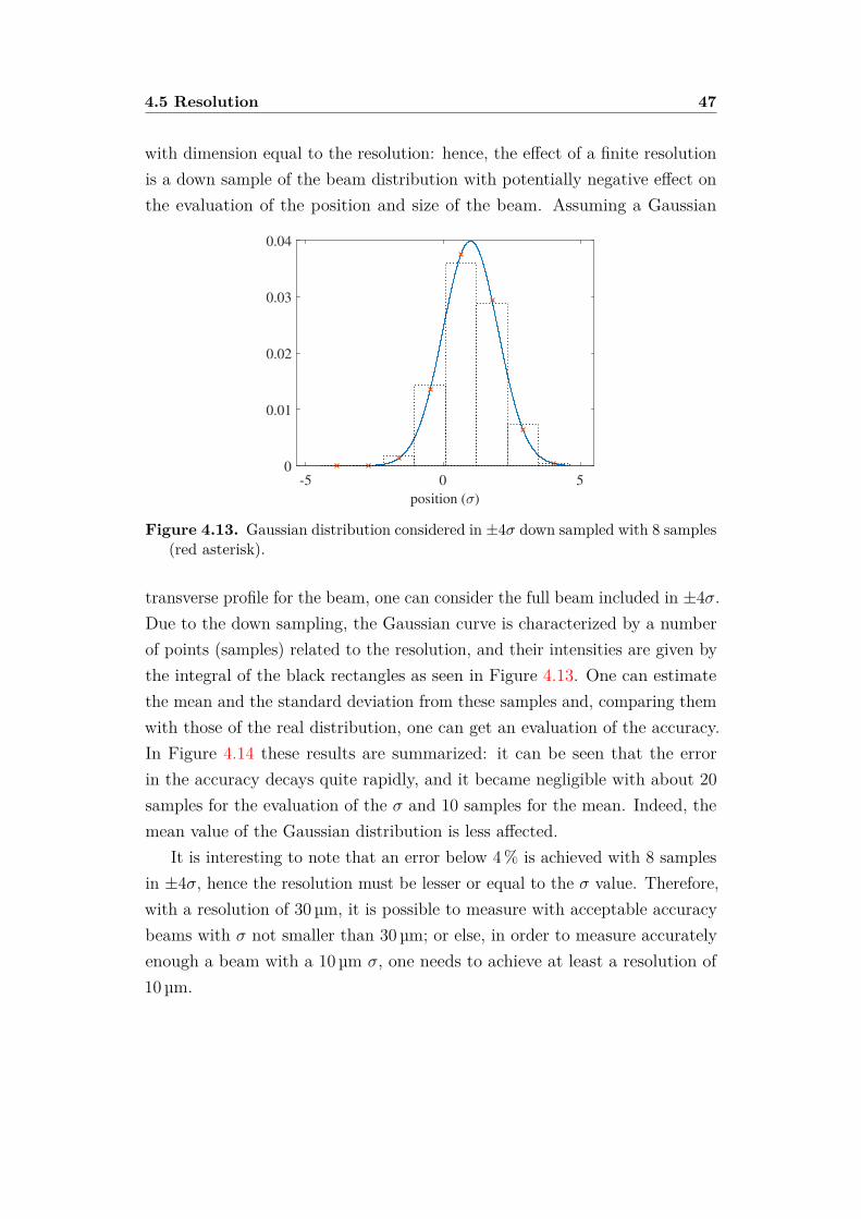
4.5 Resolution 47
with dimension equal to the resolution: hence, the effect of a finite resolutionis a down sample of the beam distribution with potentially negative effect onthe evaluation of the position and size of the beam. Assuming a Gaussian
-5 0 5
position ( )
0
0.01
0.02
0.03
0.04
Figure 4.13. Gaussian distribution considered in ±4σ down sampled with 8 samples(red asterisk).
transverse profile for the beam, one can consider the full beam included in ±4σ.Due to the down sampling, the Gaussian curve is characterized by a numberof points (samples) related to the resolution, and their intensities are given bythe integral of the black rectangles as seen in Figure 4.13. One can estimatethe mean and the standard deviation from these samples and, comparing themwith those of the real distribution, one can get an evaluation of the accuracy.In Figure 4.14 these results are summarized: it can be seen that the errorin the accuracy decays quite rapidly, and it became negligible with about 20samples for the evaluation of the σ and 10 samples for the mean. Indeed, themean value of the Gaussian distribution is less affected.
It is interesting to note that an error below 4 % is achieved with 8 samplesin ±4σ, hence the resolution must be lesser or equal to the σ value. Therefore,with a resolution of 30 µm, it is possible to measure with acceptable accuracybeams with σ not smaller than 30 µm; or else, in order to measure accuratelyenough a beam with a 10 µm σ, one needs to achieve at least a resolution of10 µm.

4.5 Resolution 48
0 5 10 15 20
# Samples in 4
-15
-10
-5
0
5
10
15
20
Rel
ativ
e E
rror
(%) 8 samples
Figure 4.14. Accuracy relative error of the mean µ (red) and the σ (blue) (andrelative error bars) of a Gaussian distribution as a function of the number ofsamples achieved in ±4σ (averaged over 300 measurements). The green dot-dashline represents the 8 samples case.
4.5.1 Calibration Procedure
In the diagnostic modules installed, a line grid is used for calibrationpurpose, instead of the USAF target; these line grids (i.e. line spacing of 2 mm)are directly lithographed in the OTR screen itself. A Matlab routine has beendesigned for the calibration: it takes as an input the acquired image and theline spacing and, counting the pixels separation with the “findpeaks” tool, itgives the calibration as an output (see Figure 4.15).
The same Matlab routine can be used with “USAF” images: however,due to the thickness of the lines, the risetime and falltime tools are moreappropriate for the pixel calculation. These tools allow the choice of start andend of the high value as a percent of the maximum value: ideally, one shouldchoose 100% since the “USAF” grid is a square wave signal. However, due tothe finite resolution and a not perfectly “in focus” image, the slopes of therise and the fall are finite and a 100% value underestimates the size of theline; after different tests, a good value has been find in 90% as can be seen inFigure 4.16. The calibration calculated in this way are closed to the expectedfrom the theory: for instance, in the case of Figure 4.16, the magnificationcalculated is about 1 and the expected value is exactly 1 at that distance(65 cm) and with the objective used (180 mm with 2x teleconverter).
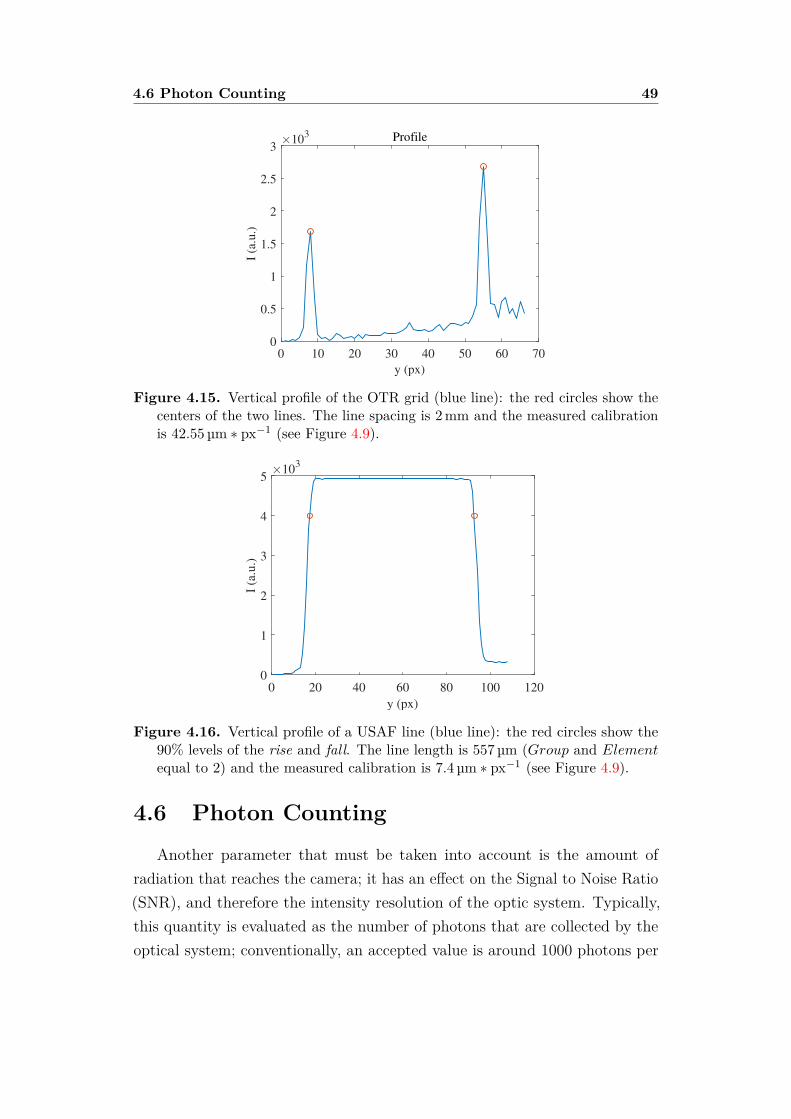
4.6 Photon Counting 49
0 10 20 30 40 50 60 70
y (px)
0
0.5
1
1.5
2
2.5
3
I (a
.u.)
103 Profile
Figure 4.15. Vertical profile of the OTR grid (blue line): the red circles show thecenters of the two lines. The line spacing is 2 mm and the measured calibrationis 42.55 µm ∗ px−1 (see Figure 4.9).
0 20 40 60 80 100 120
y (px)
0
1
2
3
4
5
I (a
.u.)
103
Figure 4.16. Vertical profile of a USAF line (blue line): the red circles show the90% levels of the rise and fall. The line length is 557 µm (Group and Elementequal to 2) and the measured calibration is 7.4 µm ∗ px−1 (see Figure 4.9).
4.6 Photon Counting
Another parameter that must be taken into account is the amount ofradiation that reaches the camera; it has an effect on the Signal to Noise Ratio(SNR), and therefore the intensity resolution of the optic system. Typically,this quantity is evaluated as the number of photons that are collected by theoptical system; conventionally, an accepted value is around 1000 photons per
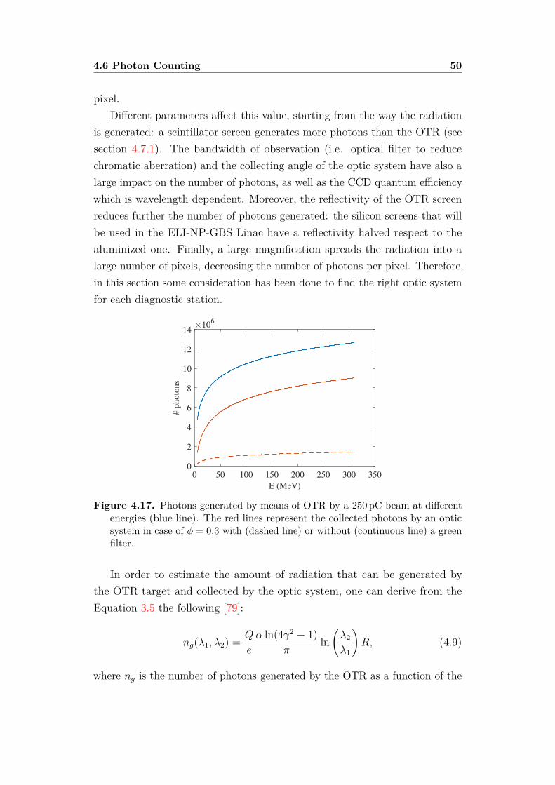
4.6 Photon Counting 50
pixel.Different parameters affect this value, starting from the way the radiation
is generated: a scintillator screen generates more photons than the OTR (seesection 4.7.1). The bandwidth of observation (i.e. optical filter to reducechromatic aberration) and the collecting angle of the optic system have also alarge impact on the number of photons, as well as the CCD quantum efficiencywhich is wavelength dependent. Moreover, the reflectivity of the OTR screenreduces further the number of photons generated: the silicon screens that willbe used in the ELI-NP-GBS Linac have a reflectivity halved respect to thealuminized one. Finally, a large magnification spreads the radiation into alarge number of pixels, decreasing the number of photons per pixel. Therefore,in this section some consideration has been done to find the right optic systemfor each diagnostic station.
0 50 100 150 200 250 300 350
E (MeV)
0
2
4
6
8
10
12
14
# p
ho
ton
s
106
Figure 4.17. Photons generated by means of OTR by a 250 pC beam at differentenergies (blue line). The red lines represent the collected photons by an opticsystem in case of φ = 0.3 with (dashed line) or without (continuous line) a greenfilter.
In order to estimate the amount of radiation that can be generated bythe OTR target and collected by the optic system, one can derive from theEquation 3.5 the following [79]:
ng(λ1, λ2) = Q
e
α ln(4γ2 − 1)π
ln(λ2
λ1
)R, (4.9)
where ng is the number of photons generated by the OTR as a function of the

4.6 Photon Counting 51
bandwidth of observation, the beam charge Q and the beam energy γ; α is thefine structure constant and R is the material reflectivity. Figure 4.17 shows thenumber of photons generated by a 250 pC bunch at different energies; it showsalso the number of photons collected assuming a collecting angle φ of 0.3 radand the possibility to use a green filter to reduce chromatic aberrations.
Figure 4.18. Collecting efficiency of an optic system as a function of the beamenergy and the collecting angle. Here, the CCD quantum efficiency and thetransmissivity of the lens is not taken into account.
The number of photons that are actually collected by the optic system,nc, are related also to the collecting angle φ = arctan (0.5D/a), where D isthe lens diameter and a is the distance between the lens and the target; thenumber of collected photons can be expressed as:
nc(Q, φ, λ1, λ2) = α
π
Q
eln(λ2
λ1
)[ln(
1 + 4γ2 tan2 φ
2
)+ cosφ
1 + γ2 sin2 φ− 1
].
(4.10)The ratio between the collected photons and the generated photons givesthe collecting efficiency of the optic system (see Figure 4.18): the efficiencyincreases with the beam energy and with the collecting angle. However, alarger collecting angle means a lens with a larger diameter or closer to thesource which may not be possible due to geometrical constraints of the machine;another possibility to increase the angle could be the opening of the diaphragm,but this is not a good idea since it increases chromaticism and other aberrationsand it reduces the depth of field.
Finally, the number of photons per pixel is given by Equation 4.11, where
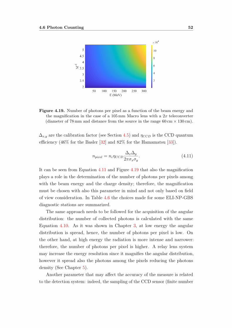
4.6 Photon Counting 52
Figure 4.19. Number of photons per pixel as a function of the beam energy andthe magnification in the case of a 105 mm Macro lens with a 2x teleconverter(diameter of 78 mm and distance from the source in the range 60 cm× 130 cm).
∆x,y are the calibration factor (see Section 4.5) and ηCCD is the CCD quantumefficiency (46% for the Basler [32] and 82% for the Hamamatsu [33]).
npixel = ncηCCD∆x∆y
2πσxσy. (4.11)
It can be seen from Equation 4.11 and Figure 4.19 that also the magnificationplays a role in the determination of the number of photons per pixels amongwith the beam energy and the charge density; therefore, the magnificationmust be chosen with also this parameter in mind and not only based on fieldof view consideration. In Table 4.6 the choices made for some ELI-NP-GBSdiagnostic stations are summarized.
The same approach needs to be followed for the acquisition of the angulardistribution: the number of collected photons is calculated with the sameEquation 4.10. As it was shown in Chapter 3, at low energy the angulardistribution is spread, hence, the number of photons per pixel is low. Onthe other hand, at high energy the radiation is more intense and narrower:therefore, the number of photons per pixel is higher. A relay lens systemmay increase the energy resolution since it magnifies the angular distribution,however it spread also the photons among the pixels reducing the photonsdensity (See Chapter 5).
Another parameter that may affect the accuracy of the measure is relatedto the detection system: indeed, the sampling of the CCD sensor (finite number
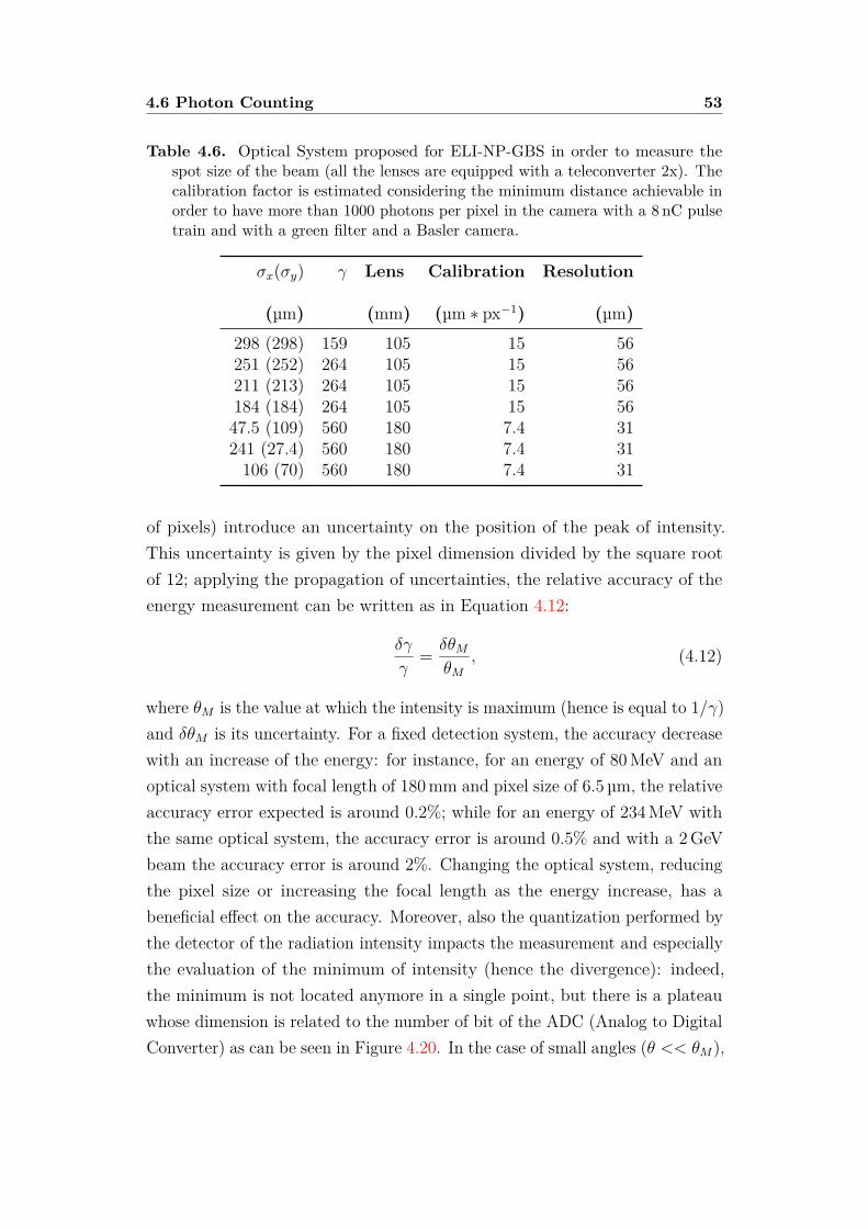
4.6 Photon Counting 53
Table 4.6. Optical System proposed for ELI-NP-GBS in order to measure thespot size of the beam (all the lenses are equipped with a teleconverter 2x). Thecalibration factor is estimated considering the minimum distance achievable inorder to have more than 1000 photons per pixel in the camera with a 8 nC pulsetrain and with a green filter and a Basler camera.
σx(σy) γ Lens Calibration Resolution
(µm) (mm) (µm ∗ px−1) (µm)298 (298) 159 105 15 56251 (252) 264 105 15 56211 (213) 264 105 15 56184 (184) 264 105 15 5647.5 (109) 560 180 7.4 31241 (27.4) 560 180 7.4 31106 (70) 560 180 7.4 31
of pixels) introduce an uncertainty on the position of the peak of intensity.This uncertainty is given by the pixel dimension divided by the square rootof 12; applying the propagation of uncertainties, the relative accuracy of theenergy measurement can be written as in Equation 4.12:
δγ
γ= δθM
θM, (4.12)
where θM is the value at which the intensity is maximum (hence is equal to 1/γ)and δθM is its uncertainty. For a fixed detection system, the accuracy decreasewith an increase of the energy: for instance, for an energy of 80 MeV and anoptical system with focal length of 180 mm and pixel size of 6.5 µm, the relativeaccuracy error expected is around 0.2%; while for an energy of 234 MeV withthe same optical system, the accuracy error is around 0.5% and with a 2 GeVbeam the accuracy error is around 2%. Changing the optical system, reducingthe pixel size or increasing the focal length as the energy increase, has abeneficial effect on the accuracy. Moreover, also the quantization performed bythe detector of the radiation intensity impacts the measurement and especiallythe evaluation of the minimum of intensity (hence the divergence): indeed,the minimum is not located anymore in a single point, but there is a plateauwhose dimension is related to the number of bit of the ADC (Analog to DigitalConverter) as can be seen in Figure 4.20. In the case of small angles (θ << θM ),
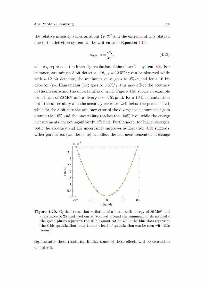
4.6 Photon Counting 54
the relative intensity varies as about (2γθ)2 and the extrema of this plateaudue to the detection system can be written as in Equation 4.13:
θmin ≈ ±√η
2γ , (4.13)
where η represents the intensity resolution of the detection system [80]. Forinstance, assuming a 8 bit detector, a θmin = 12.5%/γ can be observed whilewith a 12 bit detector, the minimum value goes to 3%/γ and for a 16 bitdetector (i.e. Hamamatsu [33]) goes to 0.8%/γ; this may affect the accuracyof the measure and the uncertainties of a fit. Figure 4.20 shows an examplefor a beam of 80 MeV and a divergence of 25 µrad: for a 16 bit quantizationboth the uncertainty and the accuracy error are well below the percent level,while for the 8 bit case the accuracy error of the divergence measurement goesaround the 10% and the uncertainty reaches the 100% level while the energymeasurements are not significantly affected. Furthermore, for higher energies,both the accuracy and the uncertainty improves as Equation 4.13 suggests.Other parameters (i.e. the noise) can affect the real measurements and change
-0.2 -0.1 0 0.1 0.2
(mrad)
0
0.5
1
1.5
2
2.5
3
3.5
I (a
.u.)
10-3
Figure 4.20. Optical transition radiation of a beam with energy of 80 MeV anddivergence of 25 µrad (red curve) zoomed around the minimum of its intensity;the green pluses represent the 16 bit quantization while the blue dots representthe 8 bit quantization (only the first level of quantization can be seen with thiszoom).
significantly these resolution limits: some of these effects will be treated inChapter 5.
4.7 Transition Radiation as a Diagnostic Tool 55
4.7 Transition Radiation as a Diagnostic Tool
The angular distribution of the transition radiation has been studied asa diagnostic tool for beam energy measurements; however, this radiation iswidely used also for beam profile measurements along with other devices likescintillator screens [81] or wire scanner [82].
In a typical monitor setup, the beam is imaged using standard lens op-tics, and the recorded intensity profile is a measure of the particle beamspot [83]. In conjunction with other accelerator components, it is also possibleto perform various measurements on the beam, namely: its energy and energyspread [84, 85] (with a dipole or corrector magnet), bunch length [86] (witha RF deflector), Twiss parameters [87] (by means of quadrupole scan) orin general 6D characterization on bunch phase space [88]. Such techniquesare common in conventional [30] and unconventional [89, 90] high brightnessLinacs.
Furthermore, it is possible to distinguish the profile monitors between inter-ceptive and non interceptive devices: the scintillator screens and the transitionradiation screens are interceptive device, while, for instance, diffraction radia-tion screens [91] are non interceptive. Diffraction radiation happens when thebeam pass through a slit; however, the radiation is weaker than the transitionradiation. On the other hand, transition radiation can be considered as anon interceptive technique under some circumstances: indeed, a thin foil ofaluminum (or mylar) has been used with highly energetic beam (in the GeVrange [92]). The issues are related to the electron scattering of the beam whenit passes through the material that increase the overall divergence and hencethe beam emittance: when the energy is high enough and the screen is thin(few micron), the scattering contribution can be considered negligible [93].
4.7.1 Comparison between YAG and OTR Screens
In order to perform beam profile and the other above mentioned measure-ments, also the scintillator screens are widely used; the main advantage isrelated to the higher radiation intensity. For instance, when a single electronhits a YAG screen, the number of photons that reach the CCD camera is givenby the product between the YAG photon yield and the solid angle coveredby the optical system [94]; the photon yield grows linearly with the electron
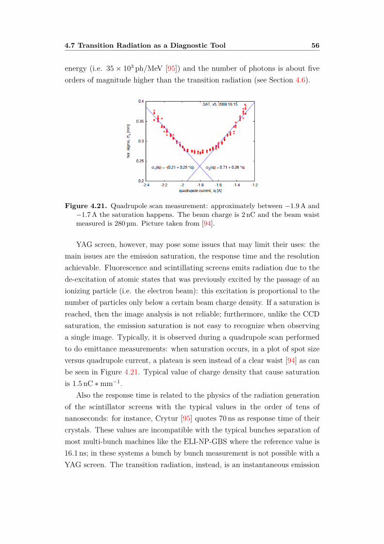
4.7 Transition Radiation as a Diagnostic Tool 56
energy (i.e. 35× 103 ph/MeV [95]) and the number of photons is about fiveorders of magnitude higher than the transition radiation (see Section 4.6).
Figure 4.21. Quadrupole scan measurement: approximately between −1.9 A and−1.7 A the saturation happens. The beam charge is 2 nC and the beam waistmeasured is 280 µm. Picture taken from [94].
YAG screen, however, may pose some issues that may limit their uses: themain issues are the emission saturation, the response time and the resolutionachievable. Fluorescence and scintillating screens emits radiation due to thede-excitation of atomic states that was previously excited by the passage of anionizing particle (i.e. the electron beam): this excitation is proportional to thenumber of particles only below a certain beam charge density. If a saturation isreached, then the image analysis is not reliable; furthermore, unlike the CCDsaturation, the emission saturation is not easy to recognize when observinga single image. Typically, it is observed during a quadrupole scan performedto do emittance measurements: when saturation occurs, in a plot of spot sizeversus quadrupole current, a plateau is seen instead of a clear waist [94] as canbe seen in Figure 4.21. Typical value of charge density that cause saturationis 1.5 nC ∗mm−1.
Also the response time is related to the physics of the radiation generationof the scintillator screens with the typical values in the order of tens ofnanoseconds: for instance, Crytur [95] quotes 70 ns as response time of theircrystals. These values are incompatible with the typical bunches separation ofmost multi-bunch machines like the ELI-NP-GBS where the reference value is16.1 ns; in these systems a bunch by bunch measurement is not possible with aYAG screen. The transition radiation, instead, is an instantaneous emission
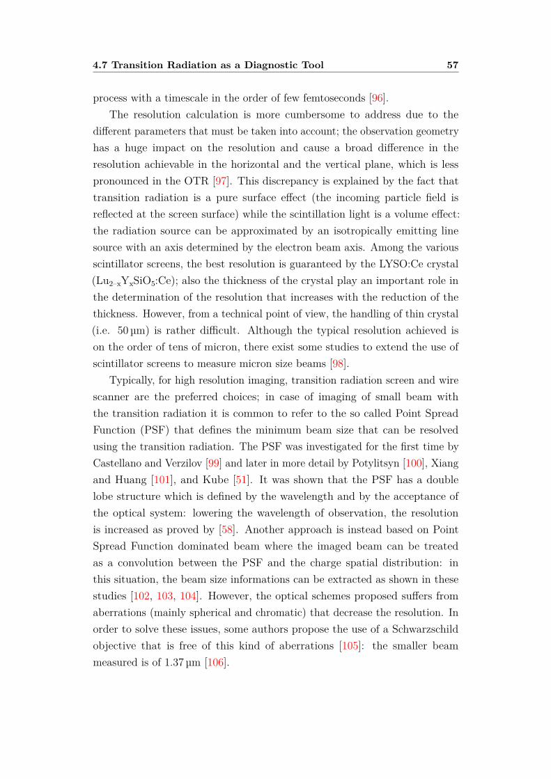
4.7 Transition Radiation as a Diagnostic Tool 57
process with a timescale in the order of few femtoseconds [96].The resolution calculation is more cumbersome to address due to the
different parameters that must be taken into account; the observation geometryhas a huge impact on the resolution and cause a broad difference in theresolution achievable in the horizontal and the vertical plane, which is lesspronounced in the OTR [97]. This discrepancy is explained by the fact thattransition radiation is a pure surface effect (the incoming particle field isreflected at the screen surface) while the scintillation light is a volume effect:the radiation source can be approximated by an isotropically emitting linesource with an axis determined by the electron beam axis. Among the variousscintillator screens, the best resolution is guaranteed by the LYSO:Ce crystal(Lu2–xYxSiO5:Ce); also the thickness of the crystal play an important role inthe determination of the resolution that increases with the reduction of thethickness. However, from a technical point of view, the handling of thin crystal(i.e. 50 µm) is rather difficult. Although the typical resolution achieved ison the order of tens of micron, there exist some studies to extend the use ofscintillator screens to measure micron size beams [98].
Typically, for high resolution imaging, transition radiation screen and wirescanner are the preferred choices; in case of imaging of small beam withthe transition radiation it is common to refer to the so called Point SpreadFunction (PSF) that defines the minimum beam size that can be resolvedusing the transition radiation. The PSF was investigated for the first time byCastellano and Verzilov [99] and later in more detail by Potylitsyn [100], Xiangand Huang [101], and Kube [51]. It was shown that the PSF has a doublelobe structure which is defined by the wavelength and by the acceptance ofthe optical system: lowering the wavelength of observation, the resolutionis increased as proved by [58]. Another approach is instead based on PointSpread Function dominated beam where the imaged beam can be treatedas a convolution between the PSF and the charge spatial distribution: inthis situation, the beam size informations can be extracted as shown in thesestudies [102, 103, 104]. However, the optical schemes proposed suffers fromaberrations (mainly spherical and chromatic) that decrease the resolution. Inorder to solve these issues, some authors propose the use of a Schwarzschildobjective that is free of this kind of aberrations [105]: the smaller beammeasured is of 1.37 µm [106].

58
Chapter 5
Energy Measurements
In Chapter 3, it was shown the theory behind the OTR and how it ispossible to use it for beam energy and beam divergence measurements.
In section 5.2 some consideration on the propagation through the opticsystem of the OTR produced by an electron beam [107] are shown: this studyhas been performed with the ZEMAX Optics Studios software [76].
Several studies has been done in order to simulate the OTR radiation inZEMAX: for instance, at CLIC [108] they study the SPF OTR for differentenergies (γ up to 4000); Wolfenden [109] studies the radiation propagationat the full optical spectrum. At SPARC_LAB the possibility to simulatethe radiation generated by the whole beam has been studied, hence takinginto account collective effects [110] (transverse spatial extension and angulardistribution).
The simulation results presented here are also validated [111] by experimen-tal data that was taken at the SPARC_LAB test facility [112] (see Section 5.1).
Finally, some of the issues related to the OTR angular distribution depen-dence on the beam energy are analyzed (see Section 5.3).
ZEMAX is a widely used software in the optics industry as a standarddesign tool. It is typically used for lens design and illumination devices. Thesoftware provides two main analysis modes: the geometrical ray tracing andthe physical optics propagation (POP) mode. The former is useful to simulatethe behavior of an optical system in the ray approximation, by neglecting anydiffraction effects related to the wave nature of the light; however, in orderto take into account diffraction effects and polarization, the POP mode ismandatory.
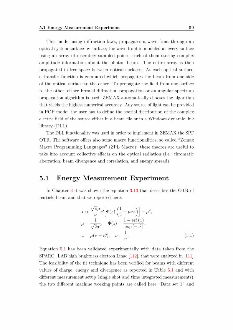
5.1 Energy Measurement Experiment 59
This mode, using diffraction laws, propagates a wave front through anoptical system surface by surface; the wave front is modeled at every surfaceusing an array of discretely sampled points, each of them storing complexamplitude information about the photon beam. The entire array is thenpropagated in free space between optical surfaces. At each optical surface,a transfer function is computed which propagates the beam from one sideof the optical surface to the other. To propagate the field from one surfaceto the other, either Fresnel diffraction propagation or an angular spectrumpropagation algorithm is used. ZEMAX automatically chooses the algorithmthat yields the highest numerical accuracy. Any source of light can be providedin POP mode: the user has to define the spatial distribution of the complexelectric field of the source either in a beam file or in a Windows dynamic linklibrary (DLL).
The DLL functionality was used in order to implement in ZEMAX the SPFOTR. The software offers also some macro functionalities, so called “ZemaxMacro Programming Languages” (ZPL Macro): these macros are useful totake into account collective effects on the optical radiation (i.e. chromaticaberration, beam divergence and correlation, and energy spread).
5.1 Energy Measurement Experiment
In Chapter 3 it was shown the equation 3.13 that describes the OTR ofparticle beam and that we reported here:
I ∝√πµ
ν<[Φ(z)
(12 + µνz
)]− µ2,
µ = 1√2σ′
, Φ(z) = 1− erf (z)exp [−z2] ,
z = µ(ν + iθ), ν = 1γ. (5.1)
Equation 5.1 has been validated experimentally with data taken from theSPARC_LAB high brightness electron Linac [112], that were analyzed in [111].The feasibility of the fit technique has been verified for beams with differentvalues of charge, energy and divergence as reported in Table 5.1 and withdifferent measurement setup (single shot and time integrated measurements);the two different machine working points are called here “Data set 1” and
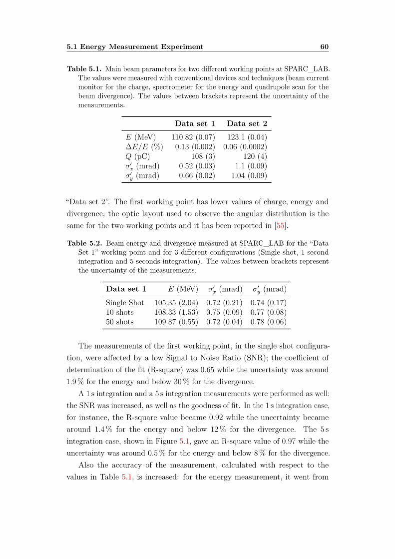
5.1 Energy Measurement Experiment 60
Table 5.1. Main beam parameters for two different working points at SPARC_LAB.The values were measured with conventional devices and techniques (beam currentmonitor for the charge, spectrometer for the energy and quadrupole scan for thebeam divergence). The values between brackets represent the uncertainty of themeasurements.
Data set 1 Data set 2E (MeV) 110.82 (0.07) 123.1 (0.04)∆E/E (%) 0.13 (0.002) 0.06 (0.0002)Q (pC) 108 (3) 120 (4)σ′x (mrad) 0.52 (0.03) 1.1 (0.09)σ′y (mrad) 0.66 (0.02) 1.04 (0.09)
“Data set 2”. The first working point has lower values of charge, energy anddivergence; the optic layout used to observe the angular distribution is thesame for the two working points and it has been reported in [55].
Table 5.2. Beam energy and divergence measured at SPARC_LAB for the “DataSet 1” working point and for 3 different configurations (Single shot, 1 secondintegration and 5 seconds integration). The values between brackets representthe uncertainty of the measurements.
Data set 1 E (MeV) σ′x (mrad) σ′y (mrad)Single Shot 105.35 (2.04) 0.72 (0.21) 0.74 (0.17)10 shots 108.33 (1.53) 0.75 (0.09) 0.77 (0.08)50 shots 109.87 (0.55) 0.72 (0.04) 0.78 (0.06)
The measurements of the first working point, in the single shot configura-tion, were affected by a low Signal to Noise Ratio (SNR); the coefficient ofdetermination of the fit (R-square) was 0.65 while the uncertainty was around1.9 % for the energy and below 30 % for the divergence.
A 1 s integration and a 5 s integration measurements were performed as well:the SNR was increased, as well as the goodness of fit. In the 1 s integration case,for instance, the R-square value became 0.92 while the uncertainty becamearound 1.4 % for the energy and below 12 % for the divergence. The 5 sintegration case, shown in Figure 5.1, gave an R-square value of 0.97 while theuncertainty was around 0.5 % for the energy and below 8 % for the divergence.
Also the accuracy of the measurement, calculated with respect to thevalues in Table 5.1, is increased: for the energy measurement, it went from

5.1 Energy Measurement Experiment 61
95 % of the single shot case to the 99 % of the 5 s integration case (in the 1 sintegration case, the accuracy was 98 %). For the divergence, instead, theaccuracy remained around a value of 90 % (see Table 5.2).
0 10 20 30 40
(mrad)
0
0.2
0.4
0.6
0.8
1
1.2
I (a
.u.)
Figure 5.1. Horizontal profile of the OTR angular distribution of a 108 pC beamwith energy of 111 MeV and divergence of 0.6 mrad (“Data Set 1” in Table 5.1).The red dots represents the data of a 5 s Integration measurement (the machineoperates at a repetition rate of 10 Hz), while the blue line is the fitting curve(Equation 5.1).
Table 5.3. Beam energy and divergence measured at SPARC_LAB for the “DataSet 2” working point and for 2 different configurations (Single shot and 1 secondintegration). The values between brackets represent the uncertainty of themeasurements.
Data set 2 E (MeV) σ′x (mrad) σ′y (mrad)Single Shot 122.13 (2.04) 1.4 (0.1) 1.3 (0.1)10 shots 123.66 (1.02) 1.3 (0.05) 1.2 (0.04)
For the second working point, the measurements were done in the singleshot configuration and with 1 s integration; in the first case, shown in figure 5.2,the R-square value was 0.82 while the uncertainty was around 1.7 % for theenergy and below 8 % for the divergence.
In the 1 s integration case, shown in figure 5.3, the R-square value was 0.98while the uncertainty was around 0.8 % for the energy and below 4 % for thedivergence.
The accuracy was 99 % for the energy and around 80 % for the divergencein the single shot case, and it increased to 99.5 % for the energy and 85 % for

5.1 Energy Measurement Experiment 62
0 10 20 30 40
(mrad)
0
0.2
0.4
0.6
0.8
1
1.2
1.4
I (a
.u.)
Figure 5.2. Horizontal profile of the OTR angular distribution of a 120 pC beamwith energy of 123 MeV and divergence of 1.1 mrad (“Data Set 2” in Table 5.1).The red dots represents the data of a single shot measurement, while the blueline is the fitting curve (Equation 5.1).
the divergence in the 1 s integration case (see Table 5.3).In order to perform a distributed energy measurement along the GBS, these
results were promising: since the OTR intensity is linearly dependent on thecharge and, due to the fact that the ELI-NP-GBS bunch charge is 250 pC,this uncertainty and accuracy results are expected for a beam energy around50 MeV.
Furthermore, the beam energy has an effect on the OTR intensity and onthe angular spread; the appropriate optics must be used in order to performan accurate fit, putting enough points between the peaks and in the tails (acommon rule of thumb is to acquire in the range θ ∈ [−3/γ : 3/γ]). This canbe done changing the focal length (a bigger focal length implies a smaller fieldof view) or the sensor pixel size; in any case, the same optic system guaranteesa wide range of energies (i.e. the one used in this experiment has a focal lengthof 400 mm and it can measure energies between 30 MeV and 3 GeV but withan increased uncertainty). Moreover, if a single shot measurement is needed,the uncertainty doubles with respect to the 1 second integration case both forthe energy and the divergence.
Hence, it can be useful to be able to simulate the radiation through an opticsystem in order to properly setup a reliable distributed energy measurement.

5.2 Energy Measurement Simulations 63
0 10 20 30 40
(mrad)
0.2
0.4
0.6
0.8
1
1.2
I (a
.u.)
Figure 5.3. Horizontal profile of the OTR angular distribution of a 120 pC beamwith energy of 123 MeV and divergence of 1.1 mrad (“Data Set 2” in Table 5.1).The red dots represents the data of a 1 s integration measurement (the machineoperates at a repetition rate of 10 Hz), while the blue line is the fitting curve(Equation 5.1).
5.2 Energy Measurement Simulations
In order to implement in ZEMAX the SPF OTR, a DLL with the approx-imation of the electric field for the OTR induced by a single electron on atarget surface [110] has been designed:
Eh = e2
4π3ε0c
2πγλK1
(2πγλr
)−J0(
2πλr)
r
cos(φ),
Ev = e2
4π3ε0c
2πγλK1
(2πγλr
)−J0(
2πλr)
r
sin(φ), (5.2)
r =√
(x− x0)2 + (y − y0)2,
φ = arctan(y − y0
x− x0
),
with x− x0 and y − y0 the two orthogonal coordinates of the target surfacemeasured from the point of electron incidence (x0, y0), γ is the relativisticLorentz factor, λ is the radiation wavelength, K1 is the modified Bessel functionof first order, and J0 is the Bessel function of zeroth order. The “h,v” indexesrepresent the horizontal and vertical polarization respectively; Figure 5.4 showsthe vertical polarized SPF OTR and its profile, in (a) and in (b), and the
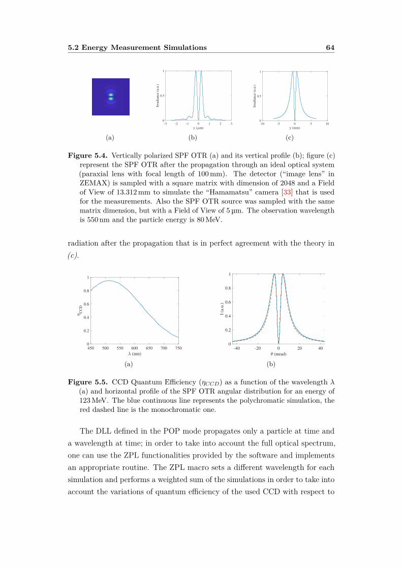
5.2 Energy Measurement Simulations 64
(a)
-3 -2 -1 0 1 2 3
y ( m)
0
0.5
1
Irra
dia
nce
(a.
u.)
(b)
-10 -5 0 5 10
y (mm)
0
0.5
1
Irra
dia
nce
(a.
u.)
(c)
Figure 5.4. Vertically polarized SPF OTR (a) and its vertical profile (b); figure (c)represent the SPF OTR after the propagation through an ideal optical system(paraxial lens with focal length of 100 mm). The detector (“image lens” inZEMAX) is sampled with a square matrix with dimension of 2048 and a Fieldof View of 13.312 mm to simulate the “Hamamatsu” camera [33] that is usedfor the measurements. Also the SPF OTR source was sampled with the samematrix dimension, but with a Field of View of 5 µm. The observation wavelengthis 550 nm and the particle energy is 80 MeV.
radiation after the propagation that is in perfect agreement with the theory in(c).
450 500 550 600 650 700 750
(nm)
0
0.2
0.4
0.6
0.8
1
CC
D
(a)
-40 -20 0 20 40
(mrad)
0
0.2
0.4
0.6
0.8
1
I (a
.u.)
(b)
Figure 5.5. CCD Quantum Efficiency (ηCCD) as a function of the wavelength λ(a) and horizontal profile of the SPF OTR angular distribution for an energy of123 MeV. The blue continuous line represents the polychromatic simulation, thered dashed line is the monochromatic one.
The DLL defined in the POP mode propagates only a particle at time anda wavelength at time; in order to take into account the full optical spectrum,one can use the ZPL functionalities provided by the software and implementsan appropriate routine. The ZPL macro sets a different wavelength for eachsimulation and performs a weighted sum of the simulations in order to take intoaccount the variations of quantum efficiency of the used CCD with respect to
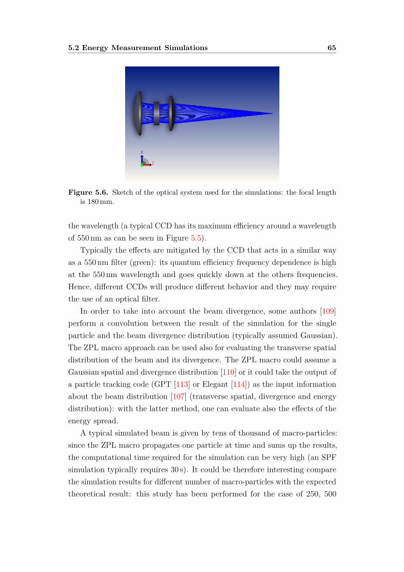
5.2 Energy Measurement Simulations 65
Figure 5.6. Sketch of the optical system used for the simulations: the focal lengthis 180 mm.
the wavelength (a typical CCD has its maximum efficiency around a wavelengthof 550 nm as can be seen in Figure 5.5).
Typically the effects are mitigated by the CCD that acts in a similar wayas a 550 nm filter (green): its quantum efficiency frequency dependence is highat the 550 nm wavelength and goes quickly down at the others frequencies.Hence, different CCDs will produce different behavior and they may requirethe use of an optical filter.
In order to take into account the beam divergence, some authors [109]perform a convolution between the result of the simulation for the singleparticle and the beam divergence distribution (typically assumed Gaussian).The ZPL macro approach can be used also for evaluating the transverse spatialdistribution of the beam and its divergence. The ZPL macro could assume aGaussian spatial and divergence distribution [110] or it could take the output ofa particle tracking code (GPT [113] or Elegant [114]) as the input informationabout the beam distribution [107] (transverse spatial, divergence and energydistribution): with the latter method, one can evaluate also the effects of theenergy spread.
A typical simulated beam is given by tens of thousand of macro-particles:since the ZPL macro propagates one particle at time and sums up the results,the computational time required for the simulation can be very high (an SPFsimulation typically requires 30 s). It could be therefore interesting comparethe simulation results for different number of macro-particles with the expectedtheoretical result: this study has been performed for the case of 250, 500
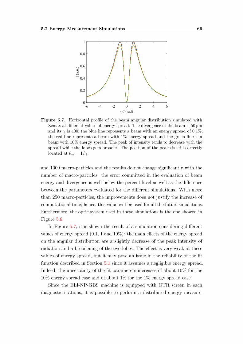
5.2 Energy Measurement Simulations 66
-6 -4 -2 0 2 4 6
(rad)
0
0.2
0.4
0.6
0.8
1
I (a
.u.)
Figure 5.7. Horizontal profile of the beam angular distribution simulated withZemax at different values of energy spread. The divergence of the beam is 50 µmand its γ is 400; the blue line represents a beam with an energy spread of 0.1%;the red line represents a beam with 1% energy spread and the green line is abeam with 10% energy spread. The peak of intensity tends to decrease with thespread while the lobes gets broader. The position of the peaks is still correctlylocated at θm = 1/γ.
and 1000 macro-particles and the results do not change significantly with thenumber of macro-particles: the error committed in the evaluation of beamenergy and divergence is well below the percent level as well as the differencebetween the parameters evaluated for the different simulations. With morethan 250 macro-particles, the improvements does not justify the increase ofcomputational time; hence, this value will be used for all the future simulations.Furthermore, the optic system used in these simulations is the one showed inFigure 5.6.
In Figure 5.7, it is shown the result of a simulation considering differentvalues of energy spread (0.1, 1 and 10%): the main effects of the energy spreadon the angular distribution are a slightly decrease of the peak intensity ofradiation and a broadening of the two lobes. The effect is very weak at thesevalues of energy spread, but it may pose an issue in the reliability of the fitfunction described in Section 5.1 since it assumes a negligible energy spread.Indeed, the uncertainty of the fit parameters increases of about 10% for the10% energy spread case and of about 1% for the 1% energy spread case.
Since the ELI-NP-GBS machine is equipped with OTR screen in eachdiagnostic stations, it is possible to perform a distributed energy measure-
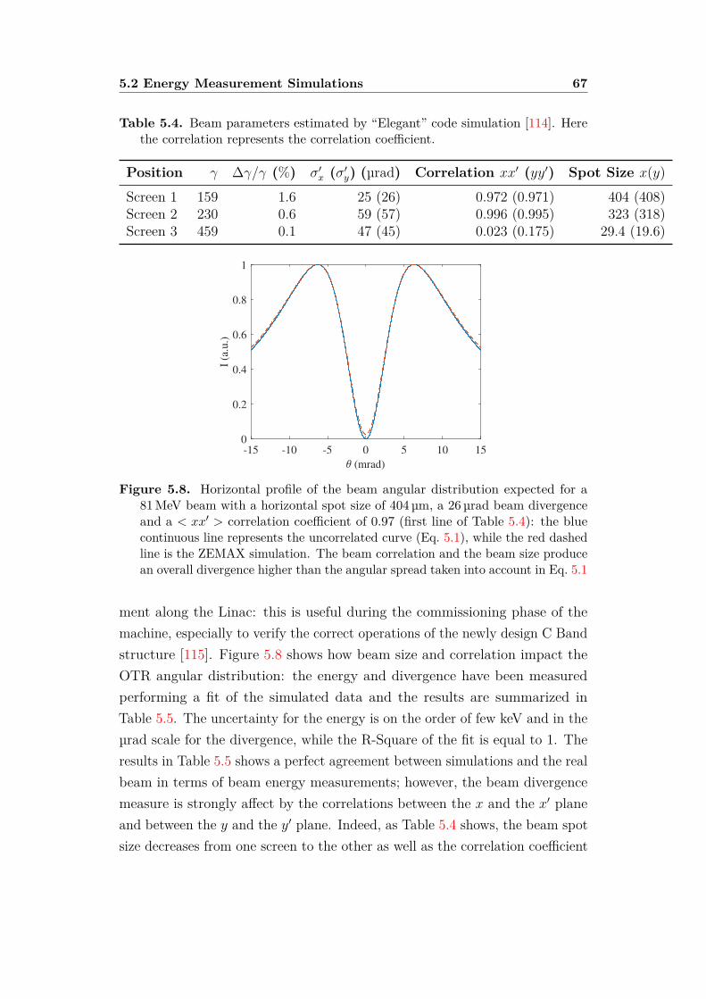
5.2 Energy Measurement Simulations 67
Table 5.4. Beam parameters estimated by “Elegant” code simulation [114]. Herethe correlation represents the correlation coefficient.
Position γ ∆γ/γ (%) σ′x (σ′y) (µrad) Correlation xx′ (yy′) Spot Size x(y)Screen 1 159 1.6 25 (26) 0.972 (0.971) 404 (408)Screen 2 230 0.6 59 (57) 0.996 (0.995) 323 (318)Screen 3 459 0.1 47 (45) 0.023 (0.175) 29.4 (19.6)
-15 -10 -5 0 5 10 15
(mrad)
0
0.2
0.4
0.6
0.8
1
I (a
.u.)
Figure 5.8. Horizontal profile of the beam angular distribution expected for a81 MeV beam with a horizontal spot size of 404 µm, a 26 µrad beam divergenceand a < xx′ > correlation coefficient of 0.97 (first line of Table 5.4): the bluecontinuous line represents the uncorrelated curve (Eq. 5.1), while the red dashedline is the ZEMAX simulation. The beam correlation and the beam size producean overall divergence higher than the angular spread taken into account in Eq. 5.1
ment along the Linac: this is useful during the commissioning phase of themachine, especially to verify the correct operations of the newly design C Bandstructure [115]. Figure 5.8 shows how beam size and correlation impact theOTR angular distribution: the energy and divergence have been measuredperforming a fit of the simulated data and the results are summarized inTable 5.5. The uncertainty for the energy is on the order of few keV and in theµrad scale for the divergence, while the R-Square of the fit is equal to 1. Theresults in Table 5.5 shows a perfect agreement between simulations and the realbeam in terms of beam energy measurements; however, the beam divergencemeasure is strongly affect by the correlations between the x and the x′ planeand between the y and the y′ plane. Indeed, as Table 5.4 shows, the beam spotsize decreases from one screen to the other as well as the correlation coefficient

5.2 Energy Measurement Simulations 68
Table 5.5. Beam energy and divergence estimated by means of fit technique usingEquation 5.1 on the Zemax simulations in the case of correlated beams. Thevalues between the parenthesis refer to the error with respect to the “Elegant”simulation results.
Position γ σ′x(µrad) σ′y (µrad)
Screen 1 159 (0.08%) 163 (560%) 158 (516%)Screen 2 230 (0.04%) 166 (183%) 172 (200%)Screen 3 459 (0.08%) 51 (8%) 49 (8%)
-15 -10 -5 0 5 10 15
(mrad)
0
0.2
0.4
0.6
0.8
1
I (a
.u.)
Figure 5.9. Horizontal profile of the beam angular distribution expected for a234 MeV beam with a horizontal spot size of 30 µm, a 47 µrad beam divergenceand a < xx′ > correlation coefficient of 0.02: the blue continuous line representsthe theoretical curve (Eq. 5.1), while the red dashed line is the ZEMAX simulation.Here, the effects of the correlation and of the beam size are negligible.
(it is close to 1 in the first 2 screens), hence the correlation gives a contributionto the overall measured divergence; furthermore, the uncertainty is affectedtoo. This is due to the fact that Equation 5.1 assume there is no correlation,hence a different equation will better fit the data. A second simulation hasbeen performed not considering the correlations: the transverse position of theparticle (x0, y0 in the Equation 5.2) is not pass through the ZPL routine. Inthis second case, there is indeed a better agreement with the theory: table 5.6summarizes these results.
In any case this simulation method proved to be very robust in the energymeasurement evaluation. Furthermore, these routines may be useful in combi-nation with some specific optic system (i.e. an array lens) in order to measurealso the beam correlation: for instance, this is particularly of interest when
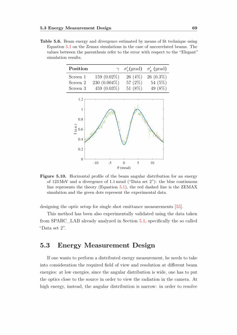
5.3 Energy Measurement Design 69
Table 5.6. Beam energy and divergence estimated by means of fit technique usingEquation 5.1 on the Zemax simulations in the case of uncorrelated beams. Thevalues between the parenthesis refer to the error with respect to the “Elegant”simulation results.
Position γ σ′x(µrad) σ′y (µrad)
Screen 1 159 (0.02%) 26 (4%) 26 (0.3%)Screen 2 230 (0.004%) 57 (2%) 54 (5%)Screen 3 459 (0.03%) 51 (8%) 49 (8%)
-10 -5 0 5 10
(mrad)
0
0.2
0.4
0.6
0.8
1
1.2
I (a
.u.)
Figure 5.10. Horizontal profile of the beam angular distribution for an energyof 123 MeV and a divergence of 1.1 mrad (“Data set 2”): the blue continuousline represents the theory (Equation 5.1), the red dashed line is the ZEMAXsimulation and the green dots represent the experimental data.
designing the optic setup for single shot emittance measurements [55].This method has been also experimentally validated using the data taken
from SPARC_LAB already analyzed in Section 5.1, specifically the so called“Data set 2”.
5.3 Energy Measurement Design
If one wants to perform a distributed energy measurement, he needs to takeinto consideration the required field of view and resolution at different beamenergies: at low energies, since the angular distribution is wide, one has to putthe optics close to the source in order to view the radiation in the camera. Athigh energy, instead, the angular distribution is narrow: in order to resolve
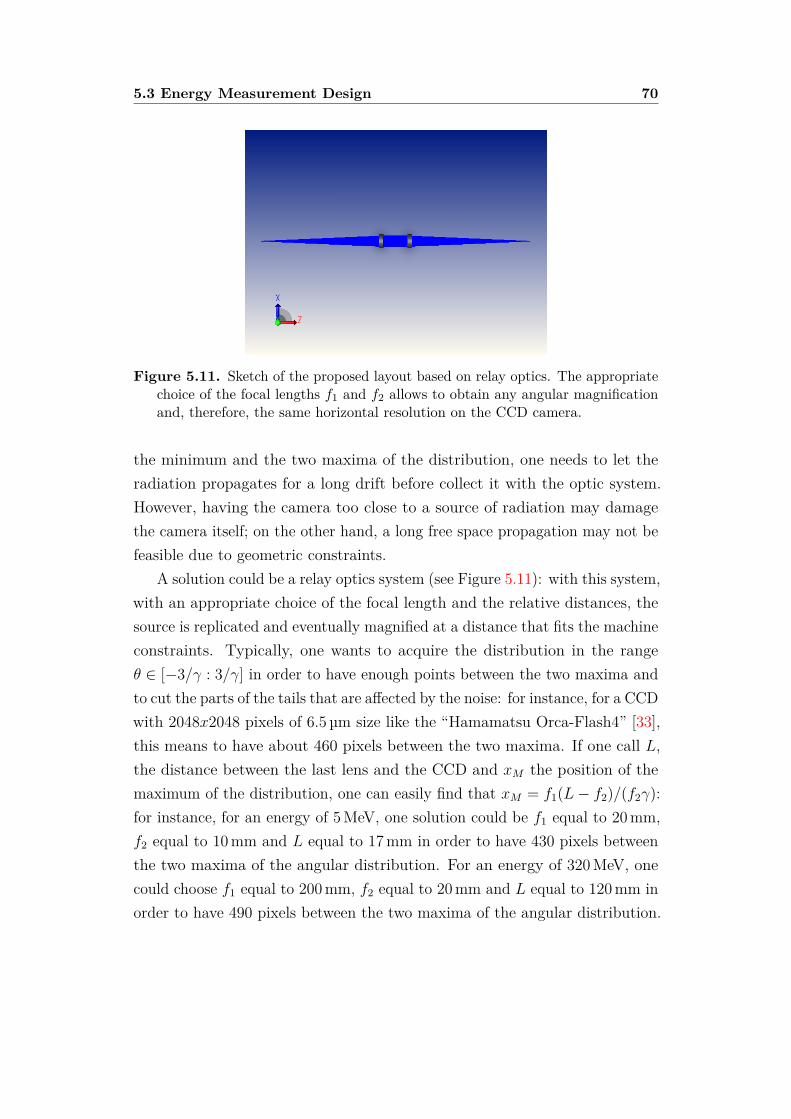
5.3 Energy Measurement Design 70
Figure 5.11. Sketch of the proposed layout based on relay optics. The appropriatechoice of the focal lengths f1 and f2 allows to obtain any angular magnificationand, therefore, the same horizontal resolution on the CCD camera.
the minimum and the two maxima of the distribution, one needs to let theradiation propagates for a long drift before collect it with the optic system.However, having the camera too close to a source of radiation may damagethe camera itself; on the other hand, a long free space propagation may not befeasible due to geometric constraints.
A solution could be a relay optics system (see Figure 5.11): with this system,with an appropriate choice of the focal length and the relative distances, thesource is replicated and eventually magnified at a distance that fits the machineconstraints. Typically, one wants to acquire the distribution in the rangeθ ∈ [−3/γ : 3/γ] in order to have enough points between the two maxima andto cut the parts of the tails that are affected by the noise: for instance, for a CCDwith 2048x2048 pixels of 6.5 µm size like the “Hamamatsu Orca-Flash4” [33],this means to have about 460 pixels between the two maxima. If one call L,the distance between the last lens and the CCD and xM the position of themaximum of the distribution, one can easily find that xM = f1(L− f2)/(f2γ):for instance, for an energy of 5 MeV, one solution could be f1 equal to 20 mm,f2 equal to 10 mm and L equal to 17 mm in order to have 430 pixels betweenthe two maxima of the angular distribution. For an energy of 320 MeV, onecould choose f1 equal to 200 mm, f2 equal to 20 mm and L equal to 120 mm inorder to have 490 pixels between the two maxima of the angular distribution.
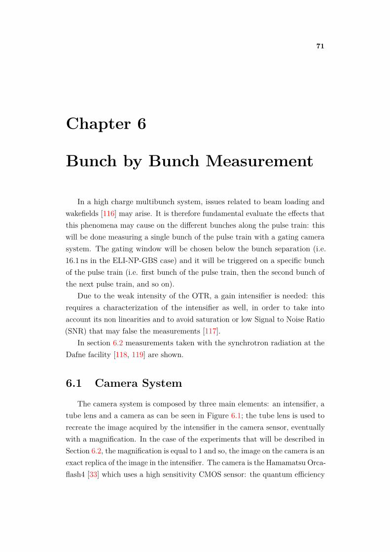
71
Chapter 6
Bunch by Bunch Measurement
In a high charge multibunch system, issues related to beam loading andwakefields [116] may arise. It is therefore fundamental evaluate the effects thatthis phenomena may cause on the different bunches along the pulse train: thiswill be done measuring a single bunch of the pulse train with a gating camerasystem. The gating window will be chosen below the bunch separation (i.e.16.1 ns in the ELI-NP-GBS case) and it will be triggered on a specific bunchof the pulse train (i.e. first bunch of the pulse train, then the second bunch ofthe next pulse train, and so on).
Due to the weak intensity of the OTR, a gain intensifier is needed: thisrequires a characterization of the intensifier as well, in order to take intoaccount its non linearities and to avoid saturation or low Signal to Noise Ratio(SNR) that may false the measurements [117].
In section 6.2 measurements taken with the synchrotron radiation at theDafne facility [118, 119] are shown.
6.1 Camera System
The camera system is composed by three main elements: an intensifier, atube lens and a camera as can be seen in Figure 6.1; the tube lens is used torecreate the image acquired by the intensifier in the camera sensor, eventuallywith a magnification. In the case of the experiments that will be described inSection 6.2, the magnification is equal to 1 and so, the image on the camera is anexact replica of the image in the intensifier. The camera is the Hamamatsu Orca-flash4 [33] which uses a high sensitivity CMOS sensor: the quantum efficiency
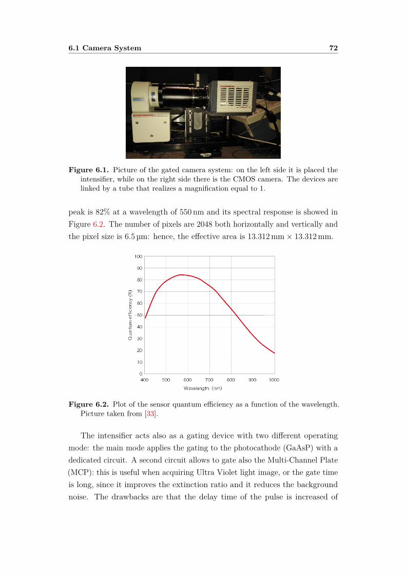
6.1 Camera System 72
Figure 6.1. Picture of the gated camera system: on the left side it is placed theintensifier, while on the right side there is the CMOS camera. The devices arelinked by a tube that realizes a magnification equal to 1.
peak is 82% at a wavelength of 550 nm and its spectral response is showed inFigure 6.2. The number of pixels are 2048 both horizontally and vertically andthe pixel size is 6.5 µm: hence, the effective area is 13.312 mm× 13.312 mm.
Figure 6.2. Plot of the sensor quantum efficiency as a function of the wavelength.Picture taken from [33].
The intensifier acts also as a gating device with two different operatingmode: the main mode applies the gating to the photocathode (GaAsP) with adedicated circuit. A second circuit allows to gate also the Multi-Channel Plate(MCP): this is useful when acquiring Ultra Violet light image, or the gate timeis long, since it improves the extinction ratio and it reduces the backgroundnoise. The drawbacks are that the delay time of the pulse is increased of

6.2 Measurements 73
Figure 6.3. Plot of the gate time window as a function of the input pulse widthcoming from the Stanford signal generator. Typically, the MCP is gated whenan improvement of the extinction ratio is needed (i.e. when observing UV lightimage). Picture taken from [33].
50 ns and the maximum repetition rate allowed is reduced to 10 kHz insteadof 30 kHz. Furthermore, as showed in Figure 6.3, the actual gate time maybe different from the input pulse width. Since the bunch separation in theELI-NP-GBS case is 16.1 ns, only the principal gate circuit is used.
The intensifier allow to set the gain of intensity in the range 600 − 990that means an actual gain between 16 dB and 43 dB with an envelope that isalmost linear in a logarithmic scale as can be seen in Figure 6.4
6.2 Measurements
In order to evaluate the effects of the Gain settings on the transversespot size measurements, a series of data have been collected at the Dafnefacility [118] using the synchrotron radiation. In a ring, the number of photonsgenerated by the beam on each turn is given by the Equation 6.1:
N(λ) =√
3 ehcγIG1
∆λλ
∆θ, (6.1)
where e is the electron charge, c is the speed of light, h is the Planck’s constant,γ is the beam Lorentz factor, I is the beam current, λ is the observationwavelength, ∆θ is the acceptance angle and G1 is called “Universal Function”.The value of the Universal function considering the Dafne critical energy [120]is 0.3; the beam in Dafne consist of a pulse train of 108 bunches with a bunchseparation of 2.7 ns, the bunch length is 100 ps and the pulse train current is
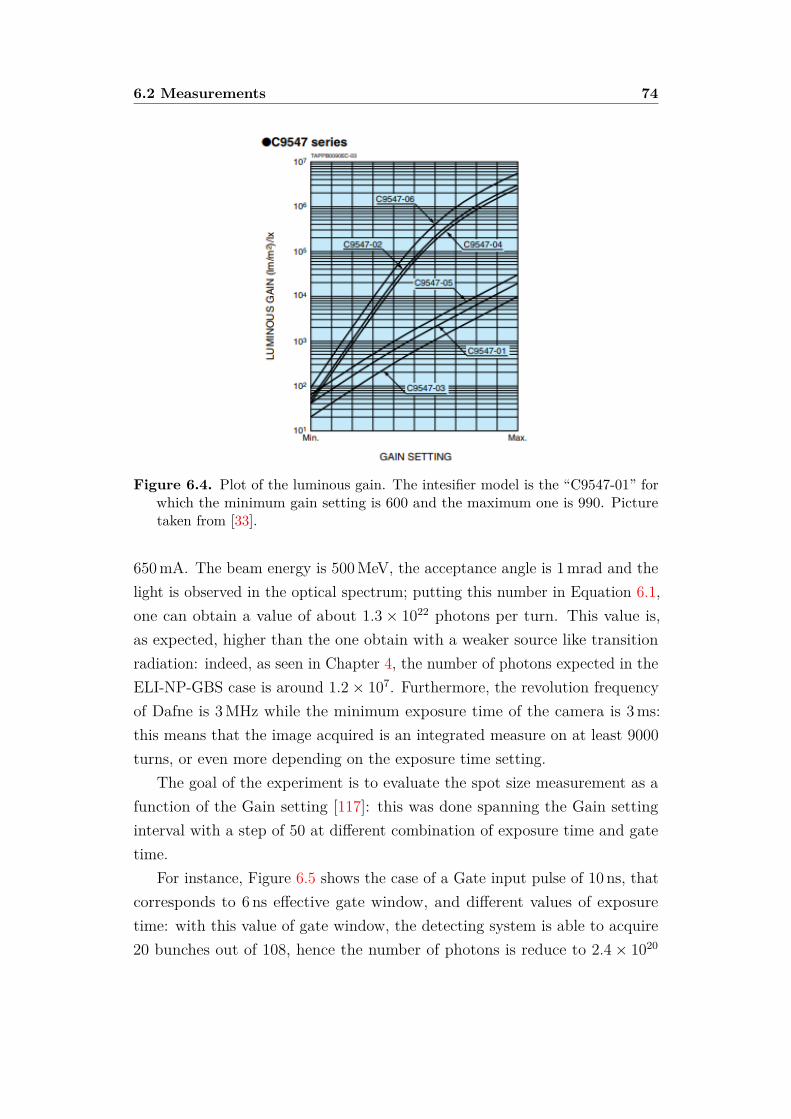
6.2 Measurements 74
Figure 6.4. Plot of the luminous gain. The intesifier model is the “C9547-01” forwhich the minimum gain setting is 600 and the maximum one is 990. Picturetaken from [33].
650 mA. The beam energy is 500 MeV, the acceptance angle is 1 mrad and thelight is observed in the optical spectrum; putting this number in Equation 6.1,one can obtain a value of about 1.3× 10²² photons per turn. This value is,as expected, higher than the one obtain with a weaker source like transitionradiation: indeed, as seen in Chapter 4, the number of photons expected in theELI-NP-GBS case is around 1.2× 10⁷. Furthermore, the revolution frequencyof Dafne is 3 MHz while the minimum exposure time of the camera is 3 ms:this means that the image acquired is an integrated measure on at least 9000turns, or even more depending on the exposure time setting.
The goal of the experiment is to evaluate the spot size measurement as afunction of the Gain setting [117]: this was done spanning the Gain settinginterval with a step of 50 at different combination of exposure time and gatetime.
For instance, Figure 6.5 shows the case of a Gate input pulse of 10 ns, thatcorresponds to 6 ns effective gate window, and different values of exposuretime: with this value of gate window, the detecting system is able to acquire20 bunches out of 108, hence the number of photons is reduce to 2.4× 10²⁰

6.2 Measurements 75
600 650 700 750 800 850 900 950
Gain Setting
1
1.1
1.2
1.3
1.4
/n
T. exp.=3ms
T. exp.=10ms
T. exp.=20ms
T. exp.=40ms
Figure 6.5. Plot of the measured spot size normalized to the expected one as afunction of the Gain setting for different values of exposure time: namely 3 ms,10 ms, 20 ms and 40 ms in blue, red, green and black line, respectively.
photons per turn. Figure 6.5 shows that with a Gain setting higher than 850,saturation arises and this impacts the beam spot measurement; also the plotof the intensity as a function of the gain shows a saturation (see Figure 6.6).It can be also noted that the exponential part of the intensity (below a gain of850) is in good agreement with the gain specification of Figure 6.4: indeed, aninterpolation of those data shows this as can be seen in Figure 6.6.
Another interesting thing to note is the behaviour for a value of the gatelength below the minimum declared in the specification (5 ns). If the inputlength is set to a value below 5 ns, or even if the gate is turn off, the behaviouris not a complete block of the light as expected: some light reaches the CCDand eventually it can be intensify. Fixing the values of exposure time (3 ms)and Gain setting (600) and changing the gate length from 5 ns to any valuebelow, or even unplugging the cable or turning off the gate, the intensity isreduce by a factor of about 7 but it does not go to the background noise level.However, two things must be noted: first, the source of intensity is ratherhigh since it comes from a large number of turns in the ring. In a Linac,the intensity expected is indeed much lower. Second, the CCD used is verysensitive to light: the use of a less sensitive camera like a “Basler” [32] withthe same beam configuration, does not show this behavior [120].
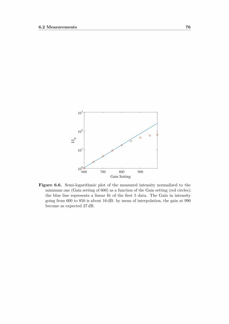
6.2 Measurements 76
600 700 800 900
Gain Setting
100
101
102
103
I/I 0
Figure 6.6. Semi-logarithmic plot of the measured intensity normalized to theminimum one (Gain setting of 600) as a function of the Gain setting (red circles);the blue line represents a linear fit of the first 5 data. The Gain in intensitygoing from 600 to 850 is about 16 dB: by mean of interpolation, the gain at 990become as expected 27 dB.

77
Chapter 7
Conclusions
This Ph.D. work has been performed in the framework of activities of theDiagnostic group of the Frascati laboratories of INFN, related to the ELINuclear Physics Gamma Beam System (ELI-NP-GBS) project.
In the ELI-NP-GBS, a high power Laser pulse is Compton scattered with anelectron beam generated through an high brightness Linac. In this way a highlypolarized, and nearly mono-energetic γ-Ray beam with a tunable energy fromabout 0.2 MeV to 19.5 MeV and a high spectral density (104 photons ∗ eV ∗ s−1)is produced. This unique γ-Ray beam has a wide range of applications fromnuclear physics to astrophysics, from medical research to homeland securityand industrial applications.
The high photon beam performances impose strong requirements on theelectron beam, thus on the diagnostic measurements setup. The Linac isrequired to achieve a normalized emittance in both directions lower than0.5 mm ∗mrad and an energy spread below 0.1%. Moreover to increase themaximum photon flux the Linac has to work in multibunch mode (32 bunchesper pulse) with a repetition rate of 100 Hz. Since the performances of the RFsystem obviously affect those of the electron beam, great care is needed in itscommissioning: hence, the availability of diagnostics measurements after eachRF module (i.e. BPMs, Beam screens) may be very useful. In particular, inthis dissertation, the possibility to perform a distributed energy measurementalong the Linac has been presented.
Overall, in the Linac 23 beam diagnostic stations are mounted, eachequipped with both YAG and OTR screen; this screens are mainly usedfor beam spot size measurements. In conjunction with other accelerator com-

78
ponents, it will also be possible to perform various measurements on thebeam, namely: its energy and energy spread (with a dipole or corrector mag-net), bunch length (with an RF Deflector), Twiss parameters (by means ofquadrupole scan) or in general 6D characterization on bunch phase space.
The high beam charge density and the multibunch mode in the ELI-NP-GBS may pose issue related to the thermo-mechanical stress due the energythat the beam deposits in the screen; a theoretical and a numerical study hasbeen performed pointing out the need to use a pure silicon screen instead of thewidely used aluminized screens. The silicon screen still allows a good qualitydiagnostic with a better resistance to thermo-mechanical stress.
The optical diagnostic stations has been characterized in terms of mag-nification and resolution achievable; a set of configurations that fits well theresolution specification for the different beam parameters along the Linachas been chosen. Namely, a “Basler Scout A640-70gm” CCD camera with alens and a teleconverter. Furthermore, in order to perform bunch by bunchmeasurements, a gating camera system has been tested and characterized.
Moreover, the OTR screens allow to retrieve the beam energy by mean ofangular distribution measurements; this, combined with the capillary presenceof the screens along the machine, allows to perform a distributed energymeasurements of the beam along the Linac.
The Transition Radiation has been characterized from the theoretical pointof view and with the optic simulation software Zemax, and validated withexperimental data taken from SPARC_LAB. The Zemax implementationallows to study the transport of the radiation trough an optic system and totake into account collective effect such as beam divergence, correlation andenergy spread or to study the impact of chromatism in the measurement.
79
Bibliography
[1] M. Marongiu et al., “Thermal behavior of the optical transition radiationscreens for the eli-np compton gamma source,” Nuclear Instrumentsand Methods in Physics Research Section A: Accelerators, Spectrometers,Detectors and Associated Equipment, 2016.
[2] F. Cioeta et al., “Thermal issues for the optical transition radiation screenfor the eli-np compton gamma source,” in 8th Int. Particle AcceleratorConf.(IPAC’17), Copenhagen, Denmark, 14-19 May, 2017, pp. 246–249.
[3] M. Marongiu et al., “Optical issues for the diagnostic stations forthe eli-np compton gamma source,” in 8th Int. Particle AcceleratorConf.(IPAC’17), Copenhagen, Denmark, 14-19 May, 2017, pp. 238–241.
[4] R. H. Milburn, “Electron scattering by an intense polarized photon field,”Physical Review Letters, vol. 10, no. 3, p. 75, 1963.
[5] F. Arutyunian et al., “The compton effect on relativistic electrons andthe possibility of obtaining high energy beams,” Phys. Letters, vol. 4,1963.
[6] L. Federici et al., “Backward compton scattering of laser light againsthigh-energy electrons: the ladon photon beam at frascati,” Il NuovoCimento B (1971-1996), vol. 59, no. 2, pp. 247–256, 1980.
[7] F. Amman et al., “Two-beam operation of the 1.5 gev electron-positronstorage ring adone,” Lettere Al Nuovo Cimento (1969-1970), vol. 1,no. 15, pp. 729–737, 1969.
[8] C. Vaccarezza et al., “The sparc_lab thomson source,” Nuclear Instru-ments and Methods in Physics Research Section A: Accelerators, Spec-

Bibliography 80
trometers, Detectors and Associated Equipment, vol. 829, pp. 237–242,2016.
[9] C. Tang et al., “Tsinghua thomson scattering x-ray source,” NuclearInstruments and Methods in Physics Research Section A: Accelerators,Spectrometers, Detectors and Associated Equipment, vol. 608, no. 1, pp.S70–S74, 2009.
[10] W. Brown et al., “Experimental characterization of an ultrafast thom-son scattering x-ray source with three-dimensional time and frequency-domain analysis,” Physical Review Special Topics-Accelerators and Beams,vol. 7, no. 6, p. 060702, 2004.
[11] F. E. Carroll et al., “Pulsed tunable monochromatic x-ray beams from acompact source: new opportunities,” American journal of roentgenology,vol. 181, no. 5, pp. 1197–1202, 2003.
[12] S. Kashiwagi et al., “Compact soft x-ray source using thomson scattering,”Journal of applied physics, vol. 98, no. 12, p. 123302, 2005.
[13] E. Miura et al., “X-ray generation via laser compton scattering usingquasi-monoenergetic electron beam driven by laser-plasma acceleration,”in AIP Conference Proceedings, vol. 1507, no. 1. AIP, 2012, pp. 304–309.
[14] C. Sun et al., “Theoretical and simulation studies of characteristics ofa compton light source,” Physical review special topics-accelerators andbeams, vol. 14, no. 4, p. 044701, 2011.
[15] E. Eggl et al., “The munich compact light source: initial performancemeasures,” Journal of synchrotron radiation, vol. 23, no. 5, pp. 1137–1142,2016.
[16] A. Bacci et al., “The Star Project,” in Proc. of International ParticleAccelerator Conference (IPAC’14), Dresden, Germany, June 15-20, 2014,pp. 2238–2241.
[17] A. Variola et al., “Thomx conceptual design report,” LAL RT, vol. 9,p. 28, 2010.
Bibliography 81
[18] E. Eggl et al., “X-ray phase-contrast tomography with a compact laser-driven synchrotron source,” Proceedings of the National Academy ofSciences, p. 201500938, 2015.
[19] R. Hajima et al., “Proposal of nondestructive radionuclide assay using ahigh-flux gamma-ray source and nuclear resonance fluorescence,” Journalof Nuclear Science and Technology, vol. 45, no. 5, pp. 441–451, 2008.
[20] T. Shizuma et al., “Nondestructive identification of isotopes using nuclearresonance fluorescence,” Review of Scientific Instruments, vol. 83, no. 1,p. 015103, 2012.
[21] V. Petrillo et al., “Photon flux and spectrum of gamma-rays comptonsources,” Nuclear Instruments and Methods in Physics Research SectionA, vol. 693, pp. 109–116, 2012.
[22] “The White Book of ELI Nuclear Physics,” http://www.eli-np.ro/documents/ELI-NP-WhiteBook.pdf.
[23] C. Vaccarezza et al., “A european proposal for the compton gamma-ray source of eli-np,” in International Particle Accelerator Conference-IPAC’12. Joint Accelerator Conferences Website, 2012, pp. 1086–1088.
[24] L. Serafini et al., “Technical Design Report EuroGammaS proposal forthe ELI-NP Gamma beam System,” EuroGammaS, Tech. Rep., 2014.
[25] “EuroGammaS Association,” http://www.e-gammas.com/.
[26] L. Serafini et al., “High intensity x/γ photon beams for nuclear physicsand photonics,” in EPJ Web of Conferences, vol. 117. Nuclear Structure,2016, p. 05002.
[27] K. Dupraz et al., “Design and optimization of a highly efficient opticalmultipass system for gamma-ray beam production from electron laserbeam compton scattering,” Physical Review Special Topics-Acceleratorsand Beams, vol. 568, no. 2, p. 033501, 2014.
[28] A. Bacci et al., “Electron linac design to drive bright Compton back-scattering gamma-ray sources,” Journal of Applied Physics, vol. 113,no. 19, p. 194508, 2013.
Bibliography 82
[29] V. Fusco et al., “Beam dynamics study of a C-band linac driven FELwith S-band photo-injector,” in Proc. of Particle Accelerator Conference(PAC’09), Vancouver, Canada, May, 2009.
[30] D. Alesini et al., “Status of the sparc project,” Nuclear Instruments andMethods in Physics Research Section A, vol. 528, no. 1, pp. 586–590,2004.
[31] M. Ferrario et al., “Experimental demonstration of emittance compensa-tion with velocity bunching,” Physical Review Letter, vol. 104, p. 054801,2010.
[32] “Basler Scout scA640-70gm,” https://www.baslerweb.com/en/products/cameras/area-scan-cameras/scout/sca640-70gm/#tab=specs.
[33] “Hamamatsu Orca-Flash 4,” https://www.hamamatsu.com/sp/sys/en/manual/C11440-22CU_IM_En.pdf.
[34] D. Alesini et al., “RF deflector design and measurements for the longitu-dinal and transverse phase space characterization at SPARC,” NuclearInstruments and Methods in Physics Research Section A: Accelerators,Spectrometers, Detectors and Associated Equipment, vol. 829, pp. 488–502, 2006.
[35] John David Jackson, Classical Electrodynamics. Wiley, 1999.
[36] http://photon-science.desy.de/research/students__teaching/primers/synchrotron_radiation/index_eng.html.
[37] G. V. Marr, Handbook on Synchrotron Radiation: Vacuum Ultravioletand Soft X-ray Processes. Elsevier, 2013, vol. 2.
[38] P. Schmüser et al., Ultraviolet and soft X-ray free-electron lasers: intro-duction to physical principles, experimental results, technological chal-lenges. Springer Science & Business Media, 2008, vol. 229.
[39] S. Corde et al., “Femtosecond x rays from laser-plasma accelerators,”Reviews of Modern Physics, vol. 85, no. 1, p. 1, 2013.
Bibliography 83
[40] V. Ginsburg et al., “Radiation of a uniformly moving electron due to itstransition from one medium into another,” Zhurnal eksperimentalnoi iteoreticheskoi fiziki, vol. 16, no. 1, pp. 15–28, 1946.
[41] M. L. Ter-Mikaelian, High energy electromagnetic processes in condensedmedia. Wiley, 1972.
[42] L. Wartski, “Etude du rayonnement de transition optique produit par desélectrons d’énergie 30 à 70 mev. application aux diagnostics de faisceauxde particules chargées,” Ph.D. dissertation, 1976.
[43] P. Rullhusen et al., Novel radiation sources using relativistic electrons:from infrared to x-rays. World Scientific, 1998, vol. 4.
[44] J. Ashley, “Transition radiation from thin foils due to non-normallyincident electrons,” Physical Review, vol. 155, no. 2, p. 208, 1967.
[45] K. Mc Donald, “Transition radiation as a beam diagnostic,” JosephHenry Laboratories, Princeton University, Princeton, NJ 08544, Tech.Rep., 1989.
[46] B. Yang, “A Design Report for the Optical Transition Radiation Imagerfor the LCLS Undulator,” SLAC, Tech. Rep., 2005.
[47] G. Garibian, “Contribution to the theory of transition radiation,” Sov.Phys. JETP, vol. 6, no. 6, p. 1079, 1958.
[48] V. Pafomov, “Radiation of a charged particle in the presence of a sepa-rating boundary,” in Nuclear Physics and Interaction of Particles withMatter. Springer, 1971, pp. 25–157.
[49] L. D. Landau et al., “The classical theory of fields,” 1971.
[50] L. Wartski et al., “Thin films on linac beams as non-destructive devicesfor particle beam intenstty, profile, centertng and energy monitors,” IEEETransactions on Nuclear Science, vol. 22, no. 3, pp. 1552–1557, 1975.
[51] G. Kube, “Imaging with optical transition radiation, transverse beamdiagnostics for the xfel,” TESLA-FEL Report, vol. 1, p. 2008, 2008.
Bibliography 84
[52] S. Casalbuoni et al., “Far-infrared transition and diffraction radiation,”Tesla Report, vol. 15, no. 2005, p. 2012, 2005.
[53] E. Chiadroni et al., “Effects of transverse electron beam size on transitionradiation angular distribution,” Nuclear Instruments and Methods inPhysics Research Section A: Accelerators, Spectrometers, Detectors andAssociated Equipment, vol. 673, pp. 56–63, 2012.
[54] V. Verzilov, Private Communication.
[55] A. Cianchi et al., “Transverse emittance diagnostics for high brightnesselectron beams,” Nuclear Instruments and Methods in Physics ResearchSection A, 2016.
[56] H. Loosy et al., “Observation of coherent optical transition radiation inthe lcls linac,” in Presented at, no. SLAC-PUB-13395, 2008.
[57] S. Wesch et al., “Observation of coherent optical transition radiationand evidence for microbunching in magnetic chicanes,” in Proc. 31st Int.Free-Electron Laser Conf., Liverpool, UK, 2009, pp. 619–622.
[58] L. G. Sukhikh et al., “Backward transition radiation in the extremeultraviolet region as a tool for the transverse beam profile diagnostic,”Physical Review Special Topics-Accelerators and Beams, vol. 17, no. 11,p. 112805, 2014.
[59] B. Schmidt et al., “Longitudinal bunch diagnostics using coherent transi-tion radiation spectroscopy,” arXiv preprint arXiv:1803.00608, 2018.
[60] F. Giorgianni et al., “Tailoring of highly intense thz radiation throughhigh brightness electron beams longitudinal manipulation,” Applied Sci-ences, vol. 6, no. 2, p. 56, 2016.
[61] M. Marongiu et al., “Design issues for the optical transition radiationscreens for theeli-np compton gamma source,” in 7th International Par-ticle Accelerator Conference (IPAC’16), Busan, Korea, May 8-13, 2016,pp. 118–121.
[62] E. Bravin, “Thermal Analysis of OTR Screens for CTF3,” CERN, Geneva,Switzerland, Tech. Rep. CTF3-Note-019, March 2001.

Bibliography 85
[63] V. Balandin et al., “Survival and thermal heating of materials for theOTR screens at the TTF2,” 2001, unpublished.
[64] M. Ross et al., “A Very High Resolution Optical Transition RadiationBeam Profile Monitor,” in BIW2002, 2002.
[65] P. Piot et al., “High-current CW beam profile monitors using transitionradiation at CEBAF,” in AIP Conference Proceedings, vol. 390, no. 1.AIP, 1997, pp. 298–305.
[66] J. Frisch et al., “Electron beam diagnostics and feedback for the LCLS-II,”in Proceedings of FEL2014, Basel, Switzerland, 2014, pp. 666–671.
[67] F. Cioeta et al., “Thermal simulations for optical transition radiationscreen for eli-np compton gamma source,” in 5th Int. Beam Instrumenta-tion Conf.(IBIC’16), Barcelona, Spain, Sept. 13-18, 2016, pp. 537–540.
[68] F. Cioeta et al., “Spot size measurements in the eli-np compton gammasource,” in 5th Int. Beam Instrumentation Conf.(IBIC’16), Barcelona,Spain, Sept. 13-18, 2016, pp. 533–536.
[69] M. Marongiu et al., “Beam energy measurements with a optical transitionradiation for the eli-np compton gamma source,” in 6th Int. BeamInstrumentation Conf.(IBIC’17), Grand Rapids, MI, USA, August 20-24,2017.
[70] “Material parameters taken by Matweb,” http://www.matweb.com/.
[71] A. Variola, “Utilisation du rayonnement optique pour l’etude des car-acteristiques spatiotemporelles d’un faisceau d’electrons. Application aTTF,” Ph.D. dissertation, Universite de Paris-Sud, France, 1998.
[72] E. Bravin et al., “OTR Studies for the High Charge CTF3 Beam,” inParticle Accelerator Conference, PAC 2003. Proceedings of, vol. 4. IEEE,2003, pp. 2464–2466.
[73] J. E. Shigley, Shigley’s mechanical engineering design. Tata McGraw-HillEducation, 2011.
[74] G. Yahr, “Fatigue design curves for 6061-t6 aluminum,” vol. 45221, pp.1–15, 1993.
Bibliography 86
[75] M. J. Kirkham, “Advances in ultra-high cycle fatigue,” 2002.
[76] “Zemax Optic Studios,” https://www.zemax.com/products/opticstudio.
[77] A. Giribono et al., “6d phase space electron beam analysis and machinesensitivity studies for eli-np gbs,” Nuclear Instruments and Methods inPhysics Research Section A, vol. 829, pp. 274–277, 2016.
[78] “Thorlabs app note: “resolution test targets”,” https://www.thorlabs.com/newgrouppage9.cfm?objectgroup_id=4338.
[79] B. Yang, “A design report for the optical transition radiation imagerfor the lcls undulator,” SLAC National Accelerator Laboratory (SLAC),Tech. Rep., 2010.
[80] X. Z. Qiu et al., “Proposal for using optical transition radiation for elec-tron beam alignment and emittance measurement for the free emittancemeasurement for the free electron laser experiments at atf,” BrookhavenNational Lab., Tech. Rep., 1994.
[81] C. Wiebers et al., “Scintillating screen monitors for transverse electronbeam profile diagnostics at the european xfel,” proceedings of IBIC, 2013.
[82] S. T. Boogert et al., “Micron-scale laser-wire scanner for the kek ac-celerator test facility extraction line,” Physical Review Special Topics-Accelerators and Beams, vol. 13, no. 12, p. 122801, 2010.
[83] W. Graves et al., “A high resolution electron beam profile monitor andits applications,” in AIP Conference Proceedings, vol. 451, no. 1. AIP,1998, pp. 206–213.
[84] K. Nakamura et al., “Broadband single-shot electron spectrometer for gev-class laser-plasma-based accelerators,” Review of Scientific Instruments,vol. 79, no. 5, p. 053301, 2008.
[85] Y. Glinec et al., “Absolute calibration for a broad range single shotelectron spectrometer,” Review of scientific instruments, vol. 77, no. 10,p. 103301, 2006.

Bibliography 87
[86] D. Filippetto et al., “Phase space analysis of velocity bunched beams,”Physical Review Special Topics-Accelerators and Beams, vol. 14, no. 9, p.092804, 2011.
[87] A. Mostacci et al., “Chromatic effects in quadrupole scan emittancemeasurements,” Physical Review Special Topics-Accelerators and Beams,vol. 15, no. 8, p. 082802, 2012.
[88] A. Cianchi et al., “Six-dimensional measurements of trains of high bright-ness electron bunches,” Physical Review Special Topics-Accelerators andBeams, vol. 18, no. 8, p. 082804, 2015.
[89] P. Antici et al., “Laser-driven electron beamlines generated by couplinglaser-plasma sources with conventional transport systems,” Journal ofApplied Physics, vol. 112, no. 4, p. 044902, 2012.
[90] A. R. Rossi et al., “The external-injection experiment at the sparc_labfacility,” Nuclear Instruments and Methods in Physics Research SectionA, vol. 740, pp. 60–66, 2014.
[91] M. Castellano, “A new non-intercepting beam size diagnostics usingdiffraction radiation from a slit,” Nuclear Instruments and Methods inPhysics Research Section A: Accelerators, Spectrometers, Detectors andAssociated Equipment, vol. 394, no. 3, pp. 275–280, 1997.
[92] P. Catravas et al., “Beam profile measurement at 30 gev using opticaltransition radiation,” 1999.
[93] C. Thomas et al., “Single shot emittance measurement from beam sizemeasurement in a drift section,” in Proceedings of the 1st InternationalParticle Accelerator Conference, 2010, p. 1167.
[94] U. Iriso et al., “Experience with yag and otr screens at alba,” SAT, vol. 5,no. 2008.10, p. 15, 2009.
[95] “Yag screen,” http://www.crytur.cz/materials/yagce/.
[96] A. Lumpkin, “Time-resolved imaging for the aps linac beams.” ArgonneNational Lab., IL (US), Tech. Rep., 1998.
Bibliography 88
[97] G. Kube et al., “Inorganic scintillators for particle beam profile diagnos-tics of highly brilliant and highly energetic electron beams,” Proceedingsof IPAC2012, New Orleans, Lousiana, USA, vol. 28, 2012.
[98] G. Kube et al., “Transverse beam profile imaging of few-micrometerbeam sizes based on a scintillator screen,” 2016.
[99] M. Castellano et al., “Spatial resolution in optical transition radiationbeam diagnostics,” Physical Rewiew Special Topics - Accelerators andBeams, vol. 1, 1998.
[100] A. Potylitsyn, “Image of optical diffraction radiation (odr) source andspatial resolution of odr beam profile monitor,” in Advanced RadiationSources and Applications. Springer, 2006, pp. 149–163.
[101] D. Xiang et al., “Theoretical considerations on imaging of micron sizeelectron beam with optical transition radiation,” Nuclear Instrumentsand Methods in Physics Research Section A: Accelerators, Spectrometers,Detectors and Associated Equipment, vol. 570, no. 3, pp. 357–364, 2007.
[102] A. Aryshev et al., “Sub-micrometer resolution transverse electron beamsize measurement system based on optical transition radiation,” in IPAC2011-2nd International Particle Accelerator Conference, 2011, pp. 1964–1966.
[103] K. Kruchinin et al., “Extremely low emittance beam size diagnosticswith sub-micrometer resolution using optical transition radiation,” 2013.
[104] G. Kube et al., “Transverse beam profile diagnostics using point spreadfunction dominated imaging with dedicated de-focusing,” 2013.
[105] I. A. Artyukov, “Schwarzschild objective and similar two-mirror sys-tems,” in Short-Wavelength Imaging and Spectroscopy Sources, vol. 8678.International Society for Optics and Photonics, 2012, p. 86780A.
[106] G. Kube et al., “Micron-scale vertical beam size measurements based ontransition radiation imaging with a schwarzschild objective,” 2016.
[107] M. Marongiu et al., “Design of the diagnostic stations for the eli-npcompton gamma source,” in 9th Int. Particle Accelerator Conf.(IPAC’18),Vancouver, BC, Canada, April 29-May 4, 2018, 2018, pp. 2173–2176.
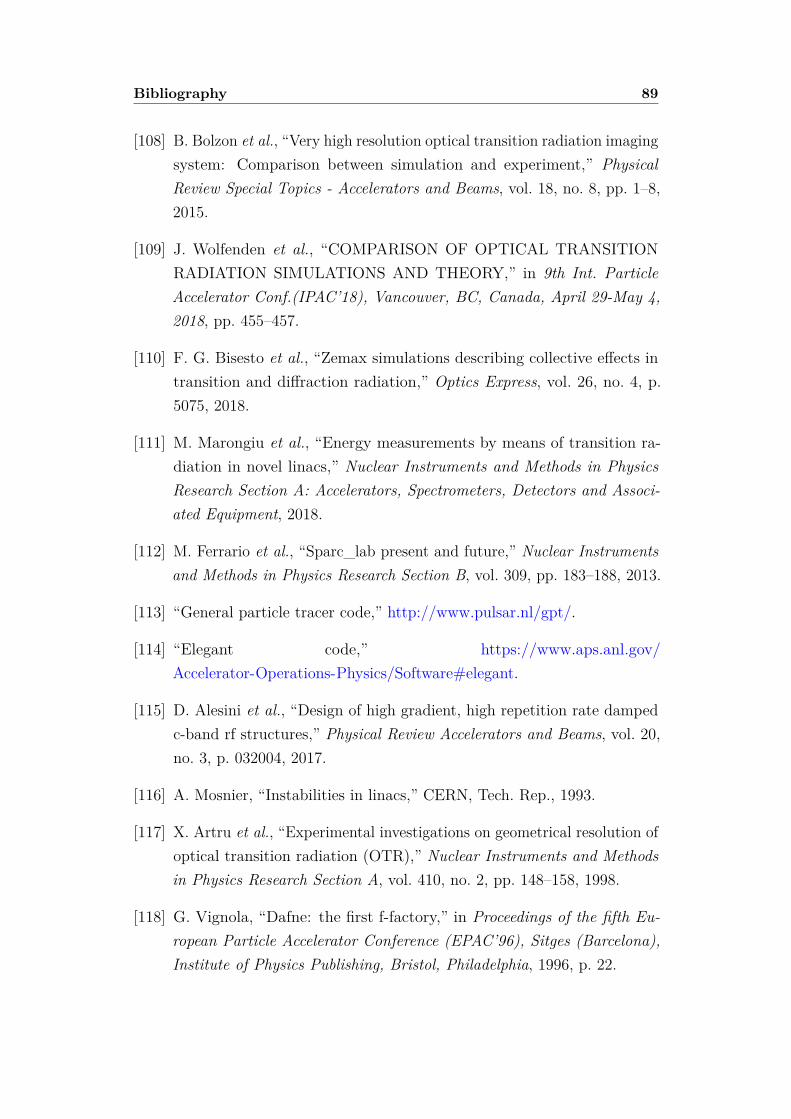
Bibliography 89
[108] B. Bolzon et al., “Very high resolution optical transition radiation imagingsystem: Comparison between simulation and experiment,” PhysicalReview Special Topics - Accelerators and Beams, vol. 18, no. 8, pp. 1–8,2015.
[109] J. Wolfenden et al., “COMPARISON OF OPTICAL TRANSITIONRADIATION SIMULATIONS AND THEORY,” in 9th Int. ParticleAccelerator Conf.(IPAC’18), Vancouver, BC, Canada, April 29-May 4,2018, pp. 455–457.
[110] F. G. Bisesto et al., “Zemax simulations describing collective effects intransition and diffraction radiation,” Optics Express, vol. 26, no. 4, p.5075, 2018.
[111] M. Marongiu et al., “Energy measurements by means of transition ra-diation in novel linacs,” Nuclear Instruments and Methods in PhysicsResearch Section A: Accelerators, Spectrometers, Detectors and Associ-ated Equipment, 2018.
[112] M. Ferrario et al., “Sparc_lab present and future,” Nuclear Instrumentsand Methods in Physics Research Section B, vol. 309, pp. 183–188, 2013.
[113] “General particle tracer code,” http://www.pulsar.nl/gpt/.
[114] “Elegant code,” https://www.aps.anl.gov/Accelerator-Operations-Physics/Software#elegant.
[115] D. Alesini et al., “Design of high gradient, high repetition rate dampedc-band rf structures,” Physical Review Accelerators and Beams, vol. 20,no. 3, p. 032004, 2017.
[116] A. Mosnier, “Instabilities in linacs,” CERN, Tech. Rep., 1993.
[117] X. Artru et al., “Experimental investigations on geometrical resolution ofoptical transition radiation (OTR),” Nuclear Instruments and Methodsin Physics Research Section A, vol. 410, no. 2, pp. 148–158, 1998.
[118] G. Vignola, “Dafne: the first f-factory,” in Proceedings of the fifth Eu-ropean Particle Accelerator Conference (EPAC’96), Sitges (Barcelona),Institute of Physics Publishing, Bristol, Philadelphia, 1996, p. 22.

Bibliography 90
[119] A. Ghigo et al., “Daφne beam instrumentation,” in AIP ConferenceProceedings, vol. 451, no. 1. AIP, 1998, pp. 183–190.
[120] A. Stella, Private Communication.

91
List of Figures
2.1 Sketch of Compton scattering of an electron and a photon in thelaboratory frame: the electron is moving along the ze directionwhile the incident photon is propagating along the directiongiven by the polar angle θi and the azimuthal angle φi. Thecollision happens at the origin of the coordinate system, and thescattered γ ray propagates in the direction given by the polarangle θf and the azimuthal angle φf . θp is the angle between themomenta of incident and scattered photons, while the electronafter the collision is not shown in the figure. . . . . . . . . . . 7
2.2 ELI-NP-GBS layout. . . . . . . . . . . . . . . . . . . . . . . . 12
3.1 Scheme of the radiation generation for an electron with a generictrajectory r(t). . . . . . . . . . . . . . . . . . . . . . . . . . . 17
3.2 Scheme of the Lorentz transformation. Picture taken from [36]. 183.3 Scheme of the transition radiation generation. Picture taken
from[46]. . . . . . . . . . . . . . . . . . . . . . . . . . . . . . . 183.4 Transition Radiation for different energy: the intensities are
normalized to the highest intensity value; the gray dot-dashedline represents the value θM = 1/γ where the peaks of thedistributions are located. The blue line represents a γ equal to20, the red one a γ equal to 40, the green line 60, the black one80 and the cyan line represents a γ equal to 100. The peak ofthe intensity scales with the square of the energy. . . . . . . . 20

List of Figures 92
3.5 Theoretical backward transition radiation patterns at differentenergies of the incident electron (incidence angle of 45°). Theblue curve represents an electron energy of 10 MeV; the red linerepresents the case of 100 MeV and the green line represents anenergy of 1 GeV. . . . . . . . . . . . . . . . . . . . . . . . . . 22
3.6 Geometry for a transition radiation screen of radius a and anobservation screen placed at a distance D. Picture taken from [52]. 23
3.7 Near field optical transition radiation calculated according toEquation 3.8: the energy is 20 GeV (the maximum energy ofXFEL) and the observation wavelength is 500 nm. Three differ-ent distance where considered: 12.19 m, 121.9 m and 1219 m. . 23
3.8 The correction factor T (ω, θ) plotted as a function of θ. Thescreen radius is 3 cm, the frequency is 1 THz and γ is equal to 300. 24
3.9 Transition Radiation curve according to Equation 3.9 for a γequal to 100 and two different frequency: a 1 THz radiation inthe blue line and a 560 THz radiation (green light) in the red line. 25
3.10 Transition Radiation for a 234 MeV energy and two differentvalues of divergence: 0.1 mrad in the blue line and a 1 mrad inthe red line. . . . . . . . . . . . . . . . . . . . . . . . . . . . . 26
3.11 Values of divergence that corresponds to a visibility of 0.1 as afunction of the energy. The red circles represent some examplesof beam energy and divergence: for a beam energy of 80 MeV,the divergence must be below 5 mrad; for a beam energy of234 MeV, the divergence must be below 2 mrad, while for abeam energy of 1.5 GeV, the divergence must be below 0.3 mrad. 28
4.1 Instantaneous temperature rising as a function of the beamdimensions for two different material (aluminum and silicon)and a bunch charge of 250 pC (a). Figure (b) represents the caseof an aluminum screen and three different bunch charges (20 pC,250 pC and 400 pC). The triangles represent the values at theposition of the OTR diagnostic stations in the ELI-NP-GBSLinac (see Table 4.3). . . . . . . . . . . . . . . . . . . . . . . . 33
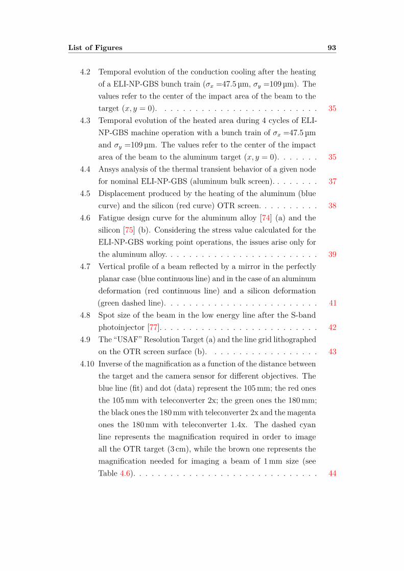
List of Figures 93
4.2 Temporal evolution of the conduction cooling after the heatingof a ELI-NP-GBS bunch train (σx =47.5 µm, σy =109 µm). Thevalues refer to the center of the impact area of the beam to thetarget (x, y = 0). . . . . . . . . . . . . . . . . . . . . . . . . . 35
4.3 Temporal evolution of the heated area during 4 cycles of ELI-NP-GBS machine operation with a bunch train of σx =47.5 µmand σy =109 µm. The values refer to the center of the impactarea of the beam to the aluminum target (x, y = 0). . . . . . . 35
4.4 Ansys analysis of the thermal transient behavior of a given nodefor nominal ELI-NP-GBS (aluminum bulk screen). . . . . . . . 37
4.5 Displacement produced by the heating of the aluminum (bluecurve) and the silicon (red curve) OTR screen. . . . . . . . . . 38
4.6 Fatigue design curve for the aluminum alloy [74] (a) and thesilicon [75] (b). Considering the stress value calculated for theELI-NP-GBS working point operations, the issues arise only forthe aluminum alloy. . . . . . . . . . . . . . . . . . . . . . . . . 39
4.7 Vertical profile of a beam reflected by a mirror in the perfectlyplanar case (blue continuous line) and in the case of an aluminumdeformation (red continuous line) and a silicon deformation(green dashed line). . . . . . . . . . . . . . . . . . . . . . . . . 41
4.8 Spot size of the beam in the low energy line after the S-bandphotoinjector [77]. . . . . . . . . . . . . . . . . . . . . . . . . . 42
4.9 The “USAF” Resolution Target (a) and the line grid lithographedon the OTR screen surface (b). . . . . . . . . . . . . . . . . . 43
4.10 Inverse of the magnification as a function of the distance betweenthe target and the camera sensor for different objectives. Theblue line (fit) and dot (data) represent the 105 mm; the red onesthe 105 mm with teleconverter 2x; the green ones the 180 mm;the black ones the 180 mm with teleconverter 2x and the magentaones the 180 mm with teleconverter 1.4x. The dashed cyanline represents the magnification required in order to imageall the OTR target (3 cm), while the brown one represents themagnification needed for imaging a beam of 1 mm size (seeTable 4.6). . . . . . . . . . . . . . . . . . . . . . . . . . . . . . 44
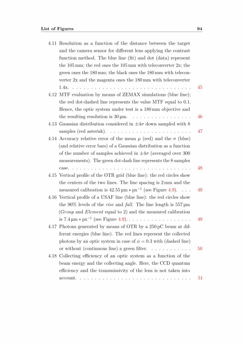
List of Figures 94
4.11 Resolution as a function of the distance between the targetand the camera sensor for different lens applying the contrastfunction method. The blue line (fit) and dot (data) representthe 105 mm; the red ones the 105 mm with teleconverter 2x; thegreen ones the 180 mm; the black ones the 180 mm with telecon-verter 2x and the magenta ones the 180 mm with teleconverter1.4x. . . . . . . . . . . . . . . . . . . . . . . . . . . . . . . . . 45
4.12 MTF evaluation by means of ZEMAX simulations (blue line);the red dot-dashed line represents the value MTF equal to 0.1.Hence, the optic system under test is a 180 mm objective andthe resulting resolution is 30 µm. . . . . . . . . . . . . . . . . 46
4.13 Gaussian distribution considered in ±4σ down sampled with 8samples (red asterisk). . . . . . . . . . . . . . . . . . . . . . . 47
4.14 Accuracy relative error of the mean µ (red) and the σ (blue)(and relative error bars) of a Gaussian distribution as a functionof the number of samples achieved in ±4σ (averaged over 300measurements). The green dot-dash line represents the 8 samplescase. . . . . . . . . . . . . . . . . . . . . . . . . . . . . . . . . 48
4.15 Vertical profile of the OTR grid (blue line): the red circles showthe centers of the two lines. The line spacing is 2 mm and themeasured calibration is 42.55 µm ∗ px−1 (see Figure 4.9). . . . 49
4.16 Vertical profile of a USAF line (blue line): the red circles showthe 90% levels of the rise and fall. The line length is 557 µm(Group and Element equal to 2) and the measured calibrationis 7.4 µm ∗ px−1 (see Figure 4.9). . . . . . . . . . . . . . . . . . 49
4.17 Photons generated by means of OTR by a 250 pC beam at dif-ferent energies (blue line). The red lines represent the collectedphotons by an optic system in case of φ = 0.3 with (dashed line)or without (continuous line) a green filter. . . . . . . . . . . . 50
4.18 Collecting efficiency of an optic system as a function of thebeam energy and the collecting angle. Here, the CCD quantumefficiency and the transmissivity of the lens is not taken intoaccount. . . . . . . . . . . . . . . . . . . . . . . . . . . . . . . 51
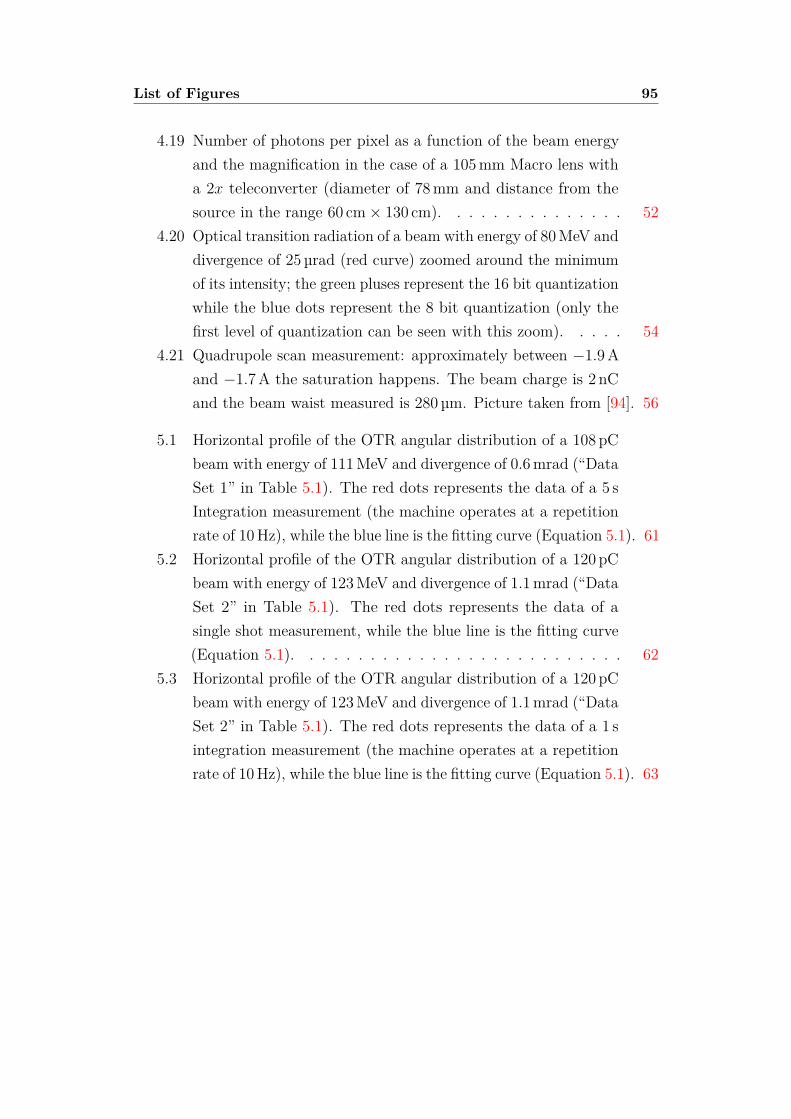
List of Figures 95
4.19 Number of photons per pixel as a function of the beam energyand the magnification in the case of a 105 mm Macro lens witha 2x teleconverter (diameter of 78 mm and distance from thesource in the range 60 cm× 130 cm). . . . . . . . . . . . . . . 52
4.20 Optical transition radiation of a beam with energy of 80 MeV anddivergence of 25 µrad (red curve) zoomed around the minimumof its intensity; the green pluses represent the 16 bit quantizationwhile the blue dots represent the 8 bit quantization (only thefirst level of quantization can be seen with this zoom). . . . . 54
4.21 Quadrupole scan measurement: approximately between −1.9 Aand −1.7 A the saturation happens. The beam charge is 2 nCand the beam waist measured is 280 µm. Picture taken from [94]. 56
5.1 Horizontal profile of the OTR angular distribution of a 108 pCbeam with energy of 111 MeV and divergence of 0.6 mrad (“DataSet 1” in Table 5.1). The red dots represents the data of a 5 sIntegration measurement (the machine operates at a repetitionrate of 10 Hz), while the blue line is the fitting curve (Equation 5.1). 61
5.2 Horizontal profile of the OTR angular distribution of a 120 pCbeam with energy of 123 MeV and divergence of 1.1 mrad (“DataSet 2” in Table 5.1). The red dots represents the data of asingle shot measurement, while the blue line is the fitting curve(Equation 5.1). . . . . . . . . . . . . . . . . . . . . . . . . . . 62
5.3 Horizontal profile of the OTR angular distribution of a 120 pCbeam with energy of 123 MeV and divergence of 1.1 mrad (“DataSet 2” in Table 5.1). The red dots represents the data of a 1 sintegration measurement (the machine operates at a repetitionrate of 10 Hz), while the blue line is the fitting curve (Equation 5.1). 63

List of Figures 96
5.4 Vertically polarized SPF OTR (a) and its vertical profile (b); fig-ure (c) represent the SPF OTR after the propagation through anideal optical system (paraxial lens with focal length of 100 mm).The detector (“image lens” in ZEMAX) is sampled with a squarematrix with dimension of 2048 and a Field of View of 13.312 mmto simulate the “Hamamatsu” camera [33] that is used for themeasurements. Also the SPF OTR source was sampled withthe same matrix dimension, but with a Field of View of 5 µm.The observation wavelength is 550 nm and the particle energyis 80 MeV. . . . . . . . . . . . . . . . . . . . . . . . . . . . . 64
5.5 CCD Quantum Efficiency (ηCCD) as a function of the wave-length λ (a) and horizontal profile of the SPF OTR angulardistribution for an energy of 123 MeV. The blue continuous linerepresents the polychromatic simulation, the red dashed line isthe monochromatic one. . . . . . . . . . . . . . . . . . . . . . 64
5.6 Sketch of the optical system used for the simulations: the focallength is 180 mm. . . . . . . . . . . . . . . . . . . . . . . . . . 65
5.7 Horizontal profile of the beam angular distribution simulatedwith Zemax at different values of energy spread. The divergenceof the beam is 50 µm and its γ is 400; the blue line represents abeam with an energy spread of 0.1%; the red line represents abeam with 1% energy spread and the green line is a beam with10% energy spread. The peak of intensity tends to decreasewith the spread while the lobes gets broader. The position ofthe peaks is still correctly located at θm = 1/γ. . . . . . . . . . 66
5.8 Horizontal profile of the beam angular distribution expected fora 81 MeV beam with a horizontal spot size of 404 µm, a 26 µradbeam divergence and a < xx′ > correlation coefficient of 0.97(first line of Table 5.4): the blue continuous line represents theuncorrelated curve (Eq. 5.1), while the red dashed line is theZEMAX simulation. The beam correlation and the beam sizeproduce an overall divergence higher than the angular spreadtaken into account in Eq. 5.1 . . . . . . . . . . . . . . . . . . . 67

List of Figures 97
5.9 Horizontal profile of the beam angular distribution expectedfor a 234 MeV beam with a horizontal spot size of 30 µm, a47 µrad beam divergence and a < xx′ > correlation coefficientof 0.02: the blue continuous line represents the theoretical curve(Eq. 5.1), while the red dashed line is the ZEMAX simulation.Here, the effects of the correlation and of the beam size arenegligible. . . . . . . . . . . . . . . . . . . . . . . . . . . . . . 68
5.10 Horizontal profile of the beam angular distribution for an energyof 123 MeV and a divergence of 1.1 mrad (“Data set 2”): theblue continuous line represents the theory (Equation 5.1), thered dashed line is the ZEMAX simulation and the green dotsrepresent the experimental data. . . . . . . . . . . . . . . . . . 69
5.11 Sketch of the proposed layout based on relay optics. The ap-propriate choice of the focal lengths f1 and f2 allows to obtainany angular magnification and, therefore, the same horizontalresolution on the CCD camera. . . . . . . . . . . . . . . . . . 70
6.1 Picture of the gated camera system: on the left side it is placedthe intensifier, while on the right side there is the CMOS camera.The devices are linked by a tube that realizes a magnificationequal to 1. . . . . . . . . . . . . . . . . . . . . . . . . . . . . . 72
6.2 Plot of the sensor quantum efficiency as a function of the wave-length. Picture taken from [33]. . . . . . . . . . . . . . . . . . 72
6.3 Plot of the gate time window as a function of the input pulsewidth coming from the Stanford signal generator. Typically, theMCP is gated when an improvement of the extinction ratio isneeded (i.e. when observing UV light image). Picture takenfrom [33]. . . . . . . . . . . . . . . . . . . . . . . . . . . . . . 73
6.4 Plot of the luminous gain. The intesifier model is the “C9547-01”for which the minimum gain setting is 600 and the maximumone is 990. Picture taken from [33]. . . . . . . . . . . . . . . . 74
6.5 Plot of the measured spot size normalized to the expected oneas a function of the Gain setting for different values of exposuretime: namely 3 ms, 10 ms, 20 ms and 40 ms in blue, red, greenand black line, respectively. . . . . . . . . . . . . . . . . . . . 75

List of Figures 98
6.6 Semi-logarithmic plot of the measured intensity normalized tothe minimum one (Gain setting of 600) as a function of theGain setting (red circles); the blue line represents a linear fit ofthe first 5 data. The Gain in intensity going from 600 to 850 isabout 16 dB: by mean of interpolation, the gain at 990 becomeas expected 27 dB. . . . . . . . . . . . . . . . . . . . . . . . . 76
99
List of Tables
2.1 Main parameters of the ELI-NP-GBS Gamma beam. . . . . . 112.2 Main parameters of the ELI-NP-GBS electron beam. . . . . . 132.3 Main parameters of the ELI-NP-GBS laser beam. . . . . . . . 13
4.1 Beam parameters for different machines. . . . . . . . . . . . . 314.2 Material property of aluminum and silicon [70]. . . . . . . . . 314.3 Instantaneous temperature increase for a 32 bunches train with
a charge of 250 pC each at the position of the OTR diagnosticstations in the ELI-NP-GBS Linac. The beam with the highercharge density has been emphasized in bold character: it causesthe higher temperature increase, hence it will be studied in moredetails. . . . . . . . . . . . . . . . . . . . . . . . . . . . . . . . 33
4.4 Von Mises Stress and maximum displacement calculated bymean of ANSYS simulation for the aluminum and the silicon inthe case of a beam spot size of 47.5 µm× 109 µm. . . . . . . . 38
4.5 Effects of the multibunching on the thermal and the mechanicalparameter of the aluminum. . . . . . . . . . . . . . . . . . . . 40
4.6 Optical System proposed for ELI-NP-GBS in order to measurethe spot size of the beam (all the lenses are equipped with ateleconverter 2x). The calibration factor is estimated consideringthe minimum distance achievable in order to have more than1000 photons per pixel in the camera with a 8 nC pulse trainand with a green filter and a Basler camera. . . . . . . . . . . 53

List of Tables 100
5.1 Main beam parameters for two different working points atSPARC_LAB. The values were measured with conventionaldevices and techniques (beam current monitor for the charge,spectrometer for the energy and quadrupole scan for the beamdivergence). The values between brackets represent the uncer-tainty of the measurements. . . . . . . . . . . . . . . . . . . . 60
5.2 Beam energy and divergence measured at SPARC_LAB for the“Data Set 1” working point and for 3 different configurations(Single shot, 1 second integration and 5 seconds integration).The values between brackets represent the uncertainty of themeasurements. . . . . . . . . . . . . . . . . . . . . . . . . . . . 60
5.3 Beam energy and divergence measured at SPARC_LAB for the“Data Set 2” working point and for 2 different configurations(Single shot and 1 second integration). The values betweenbrackets represent the uncertainty of the measurements. . . . . 61
5.4 Beam parameters estimated by “Elegant” code simulation [114].Here the correlation represents the correlation coefficient. . . . 67
5.5 Beam energy and divergence estimated by means of fit techniqueusing Equation 5.1 on the Zemax simulations in the case ofcorrelated beams. The values between the parenthesis refer tothe error with respect to the “Elegant” simulation results. . . 68
5.6 Beam energy and divergence estimated by means of fit techniqueusing Equation 5.1 on the Zemax simulations in the case ofuncorrelated beams. The values between the parenthesis referto the error with respect to the “Elegant” simulation results. . 69