Othman Boudhoum Thesis

Value Focused Inland Waterway Infrastructure Investment Decisions

A thesis submitted in partial fulfillment

of the requirements for the degree of

Master of Science in Industrial Engineering

By

Othman Boudhoum

University of Arkansas

Bachelor of Science in Industrial Engineering, 2013

July 2015

University of Arkansas

This thesis is approved for recommendation to the Graduate Council

______________________________

Dr. Heather Nachtmann

Thesis Director

_______________________________

Dr. Edward Pohl

Committee Member

_______________________________

Dr. Gregory Parnell

Committee Member

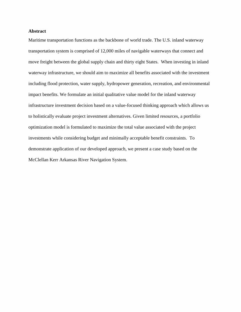
Abstract

Maritime transportation functions as the backbone of world trade. The U.S. inland waterway

transportation system is comprised of 12,000 miles of navigable waterways that connect and

move freight between the global supply chain and thirty eight States. When investing in inland

waterway infrastructure, we should aim to maximize all benefits associated with the investment

including flood protection, water supply, hydropower generation, recreation, and environmental

impact benefits. We formulate an initial qualitative value model for the inland waterway

infrastructure investment decision based on a value-focused thinking approach which allows us

to holistically evaluate project investment alternatives. Given limited resources, a portfolio

optimization model is formulated to maximize the total value associated with the project

investments while considering budget and minimally acceptable benefit constraints. To

demonstrate application of our developed approach, we present a case study based on the

McClellan Kerr Arkansas River Navigation System.

Acknowledgments

First of all, I would like to extend my gratitude and thanks to my family for their unconditional

support during the past 18 years of my education. I would like to thank my father Abdellah

Boudhoum and my mother Lalla Nezha Abouelfaraj for being always supportive and providing

whatever my siblings and I asked for. Without them, I would not be the person I am today. I

would like also to thank all the faculty and staff of the Industrial Engineering Department at the

University of Arkansas for all the help and wonderful experiences during the past 6 years at the

University of Arkansas.

Lastly, I would like to thank my advisor Dr. Heather Nachtmann for her support and help during

the past 20 months. I also would like to express my gratitude to her and to Dr. Ed Pohl and Dr.

Greg Parnell for serving on my Thesis Committee and supporting me in this research.

Dedication

I would like to dedicate this thesis to my family who have always motivated me and believed in

me. Lalla Nezha Abouelfaraj, Abdellah, Mohamed, and Salma Boudhoum, thank you for being

the awesome family that you are. I would also like to dedicate this to every faculty member at

the University of Arkansas who helped shape my academic career.

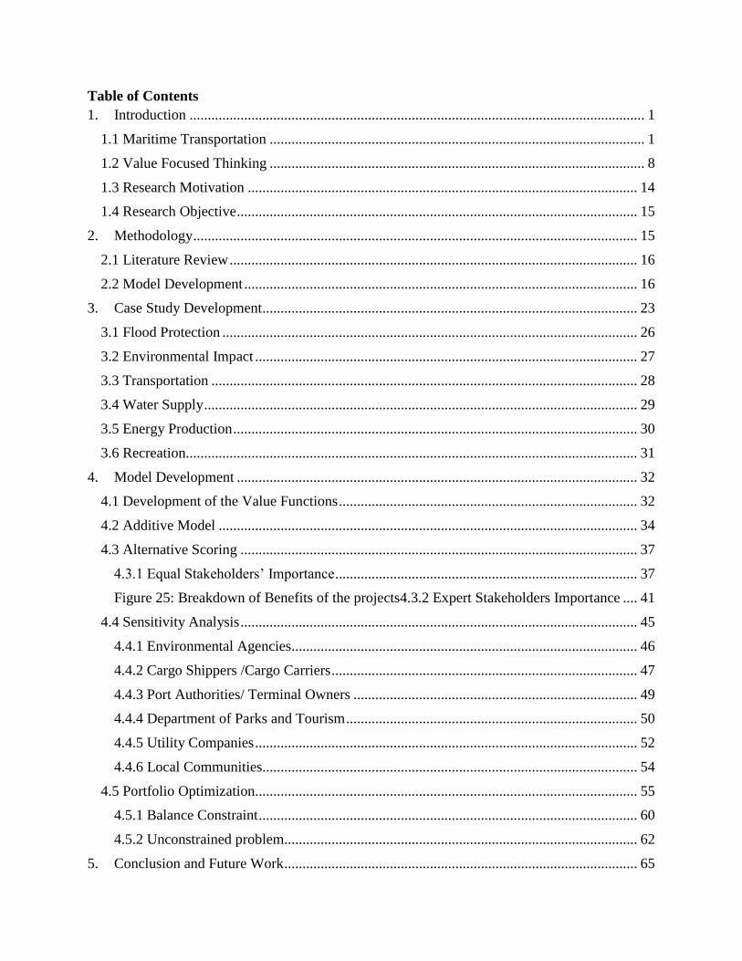
Table of Contents

1. Introduction ............................................................................................................................. 1

1.1 Maritime Transportation ....................................................................................................... 1

1.2 Value Focused Thinking ....................................................................................................... 8

1.3 Research Motivation ........................................................................................................... 14

1.4 Research Objective .............................................................................................................. 15

2. Methodology .......................................................................................................................... 15

2.1 Literature Review ................................................................................................................ 16

2.2 Model Development ............................................................................................................ 16

3. Case Study Development....................................................................................................... 23

3.1 Flood Protection .................................................................................................................. 26

3.2 Environmental Impact ......................................................................................................... 27

3.3 Transportation ..................................................................................................................... 28

3.4 Water Supply ....................................................................................................................... 29

3.5 Energy Production ............................................................................................................... 30

3.6 Recreation............................................................................................................................ 31

4. Model Development .............................................................................................................. 32

4.1 Development of the Value Functions .................................................................................. 32

4.2 Additive Model ................................................................................................................... 34

4.3 Alternative Scoring ............................................................................................................. 37

4.3.1 Equal Stakeholders’ Importance ................................................................................... 37

Figure 25: Breakdown of Benefits of the projects4.3.2 Expert Stakeholders Importance .... 41

4.4 Sensitivity Analysis ............................................................................................................. 45

4.4.1 Environmental Agencies ............................................................................................... 46

4.4.2 Cargo Shippers /Cargo Carriers .................................................................................... 47

4.4.3 Port Authorities/ Terminal Owners .............................................................................. 49

4.4.4 Department of Parks and Tourism ................................................................................ 50

4.4.5 Utility Companies ......................................................................................................... 52

4.4.6 Local Communities....................................................................................................... 54

4.5 Portfolio Optimization......................................................................................................... 55

4.5.1 Balance Constraint ........................................................................................................ 60

4.5.2 Unconstrained problem................................................................................................. 62

5. Conclusion and Future Work ................................................................................................. 65

References ..................................................................................................................................... 68

Appendix A ................................................................................................................................... 72

Appendix B: One way Sensitivity Analysis Results ..................................................................... 78

List of Figures

Figure 1: U.S import and export value by mode (Chambers, 2012) ............................................... 2

Figure 2: Freight flows by highway, railroad, and waterway (U.S. Department of Transportation,

2013) ............................................................................................................................................... 3

Figure 3: Breakdown of freight transported in inland waterways in 2010 (World Wide Inland

Navigation Network, n.d.) .............................................................................................................. 3

Figure 4: U.S. hydroelectric plants (USACE, 2013-2) ................................................................... 5

Figure 5: Efficiency of power generating alternatives (USACE, 2013-2)...................................... 6

Figure 6: Fuel-efficiency of different modes of transportation (TTI, 2012) ................................... 7

Figure 7: Comparison of cargo capacity (Iowa Department of Transportation, 2008) .................. 7

Figure 8: VFT benefits (Keeney, 1992) .......................................................................................... 9

Figure 9: VFT literature application domains (Parnell et al., 2013) ............................................. 10

Figure 10: Number of value measures surveyed in VFT literature (Parnell et al., 2013) ............. 11

Figure 11: Use of resources in VFT literature (Parnell et al., 2013) ............................................ 11

Figure 12: Steps to develop value hierarchy (Parnell, 2007) ........................................................ 16

Figure 13: Benefits of inland waterways. (Town and Country Planning Association, 2009) ...... 18

Figure 14: Objectives of the IWS infrastructure investment decision .......................................... 19

Figure 15: Basic value hierarchy .................................................................................................. 21

Figure 16: Value hierarchy including stakeholders ...................................................................... 22

Figure 17: MKARNS lock lift (King, 2012) ................................................................................. 24

Figure 18: Map of MKARNS project locations (USACE, 2005 .................................................. 25

Figure 19: 2011 tonnages (in thousand tons) through each MKARNS L/D ................................. 29

Figure 20: Flood protection value function .................................................................................. 33

Figure 21 :Transportation value function ..................................................................................... 33

Figure 22: Water supply Value Function ...................................................................................... 33

Figure 23: Energy production value function ............................................................................... 33

Figure 24: Recreation value function ............................................................................................ 34

Figure 25: Breakdown of Benefits of the projects ........................................................................ 41

Figure 26: Comparison of total project alternative Benefits using expert and equal stakeholder

importance..................................................................................................................................... 45

Figure 27: One way sensitivity analysis of environmental agencies importance ......................... 47

Figure 28: One way sensitivity analysis of cargo shippers/ cargo carriers’ importance .............. 48

Figure 29: One way sensitivity analysis of ports authorities/terminal owners’ importance ......... 50

Figure 30: One way sensitivity analysis of department of parks and tourism’ importance .......... 52

Figure 31: One way sensitivity analysis of utility companies’ importance .................................. 53

Figure 32: One way sensitivity analysis of local communities’ importance ................................ 55

Figure 33: Project efficient frontier (Cost vs Benefit) .................................................................. 60

Figure 34: Comparison of portfolio optimization outputs (no constraints vs. minimum acceptable

score of 70% ................................................................................................................................. 64

List of Tables

Table 1: Tong et al. (2013) literature assessment matrix .............................................................. 13

Table 2: Proposed methodology ................................................................................................... 16

Table 3: Benefits of inland waterways (Jacobs Engineering U.K., 2011) .................................... 17

Table 4: Types of measures preference Parnell (2007) ................................................................ 20

Table 5: Value measures used ....................................................................................................... 20

Table 6: List of case study projects, type, and state location ........................................................ 26

Table 7: MKARNS Project flood control pool storage capacity in acre-ft (USACE, 2005)

(USACE, n.d.) ............................................................................................................................... 27

Table 8: Number of endangered and threatened species for each MKARNS project (USACE,

2005) ............................................................................................................................................. 28

Table 9: Water supply MKARNS projects with yield in millions gallons per day (USACE, 2013 -

4) ................................................................................................................................................... 30

Table 10: MKARNS Projects with hydropower installed capacity in Kilowatts (USACE, 2005)31

Table 11: MKARNS projects with number of recreational visitors (USACE, 2012-2) ............... 32

Table 12: Evaluation measure for environmental impact ............................................................. 34

Table 13: Values assessments and weights for environmental agencies ...................................... 36

Table 14: Values assessments and weights for cargo shippers/cargo carriers .............................. 36

Table 15: Values assessments and weights for local communities............................................... 36

Table 16: Values assessments and weights for port authorities/ terminal owners ........................ 36

Table 17: Values assessments and weights for department of parks and tourism ........................ 37

Table 18: Values assessment and weights for utility companies .................................................. 37

Table 19: Stakeholders assessments for values and average assessment for each value .............. 38

Table 20: Results of MKARNS project VFT analysis under equal stakeholder importance ....... 39

Table 21: Expert assessments and normalized weights for stakeholder importance .................... 42

Table 22: Results of MKARNS project VFT analysis under expert stakeholder importance ...... 44

Table 23: Project modernization and maintenance costs .............................................................. 59

Table 24: Portfolio Optimization objective function, constraints, and results ............................. 61

Table 25: Optimal MKARNS project portfolio summary ............................................................ 62

Table 26: Comparison of portfolio optimization outputs (no constraints vs. minimum acceptable

score of 70% ................................................................................................................................. 63

Table 27: Optimal MKARNS project portfolio summary ............................................................ 65

Table 28: Projects single dimensional value for flood protection ................................................ 72

Table 29: Projects single dimensional value for environmental impact ....................................... 73

Table 30: Projects single dimensional value for transportation ................................................... 74

Table 31: Projects single dimensional value for water supply ..................................................... 75

Table 32: Projects single dimensional value for energy production ............................................. 76

Table 33: Projects single dimensional value for recreation .......................................................... 77

Table 34: One way sensitivity analysis of environmental agencies importance .......................... 79

Table 35: One way sensitivity analysis of cargo shippers/cargo carriers importance ................. 80

Table 36: One way sensitivity analysis of port authorities/terminal owners’ importance ............ 81

Table 37: One way sensitivity analysis of department of parks and tourism importance ............ 82

Table 38: One way sensitivity analysis of utility companies’ importance ................................... 83

Table 39: One way sensitivity analysis of local communities’ importance .................................. 84

1

1. Introduction

1.1 Maritime Transportation

Maritime transportation functions as the backbone of world trade. Approximately 80% of world

trade by volume and approximately 70% by value are transported by sea (United States

Conference on Trade and Development (UNCTAD), 2014). Seaborne trade reached a total

volume of 9.6 billion tons in 2013 accounting for a total of 500 billion ton-miles (UNCTAD,

2014). Economically developed countries’ imports accounted for 38% of total imports

transported by water, in comparison with 60% for developing countries and 2% for emerging

economies. Developing countries accounted for the majority of exports using water

transportation with 61% of total volume, and developed countries accounted for 33%

(UNCTAD, 2014).

In 2011, a total of 1.34 billion tons of waterborne freight valued at $1.73 trillion was imported to

and exported from the United States (U.S.) (Chambers, 2012). Maritime transportation

contributed more than $36 billion to the U.S. economy in 2010 and directly and indirectly

supported thirteen million jobs. In 2011, the maritime transportation system accounted for 95%

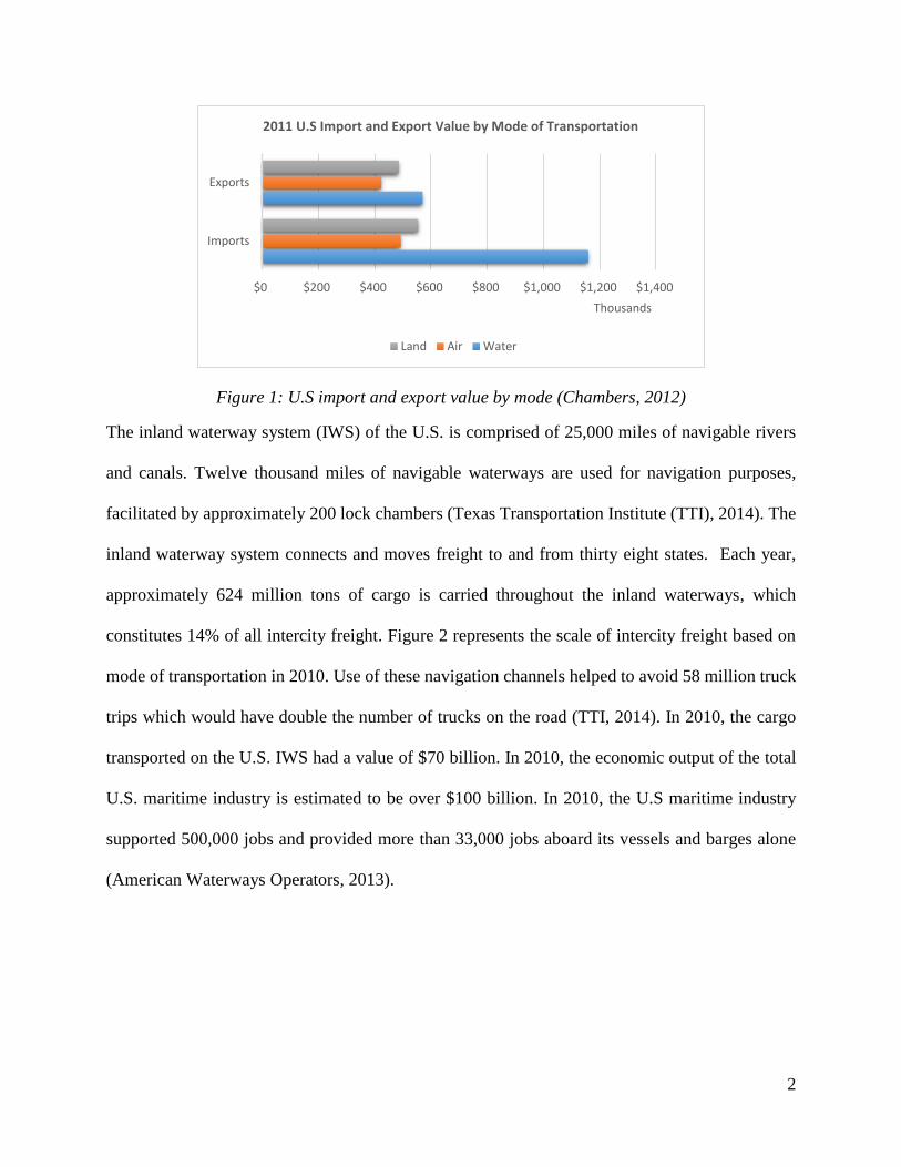
of the U.S. foreign trade by volume (Chambers, 2012). Maritime transportation accounted for

53% and 38% of U.S. import and export values as shown in Figure 1 (Chambers, 2012).

2

Figure 1: U.S import and export value by mode (Chambers, 2012)

The inland waterway system (IWS) of the U.S. is comprised of 25,000 miles of navigable rivers

and canals. Twelve thousand miles of navigable waterways are used for navigation purposes,

facilitated by approximately 200 lock chambers (Texas Transportation Institute (TTI), 2014). The

inland waterway system connects and moves freight to and from thirty eight states. Each year,

approximately 624 million tons of cargo is carried throughout the inland waterways, which

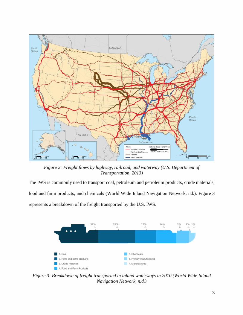
constitutes 14% of all intercity freight. Figure 2 represents the scale of intercity freight based on

mode of transportation in 2010. Use of these navigation channels helped to avoid 58 million truck

trips which would have double the number of trucks on the road (TTI, 2014). In 2010, the cargo

transported on the U.S. IWS had a value of $70 billion. In 2010, the economic output of the total

U.S. maritime industry is estimated to be over $100 billion. In 2010, the U.S maritime industry

supported 500,000 jobs and provided more than 33,000 jobs aboard its vessels and barges alone

(American Waterways Operators, 2013).

Imports

Exports

$0 $200 $400 $600 $800 $1,000 $1,200 $1,400

Thousands

2011 U.S Import and Export Value by Mode of Transportation

Land Air Water

3

Figure 2: Freight flows by highway, railroad, and waterway (U.S. Department of

Transportation, 2013)

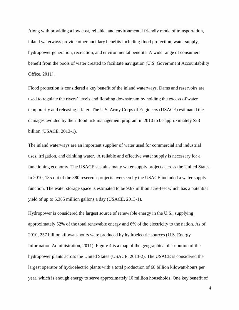
The IWS is commonly used to transport coal, petroleum and petroleum products, crude materials,

food and farm products, and chemicals (World Wide Inland Navigation Network, nd.). Figure 3

represents a breakdown of the freight transported by the U.S. IWS.

Figure 3: Breakdown of freight transported in inland waterways in 2010 (World Wide Inland

Navigation Network, n.d.)

4

Along with providing a low cost, reliable, and environmental friendly mode of transportation,

inland waterways provide other ancillary benefits including flood protection, water supply,

hydropower generation, recreation, and environmental benefits. A wide range of consumers

benefit from the pools of water created to facilitate navigation (U.S. Government Accountability

Office, 2011).

Flood protection is considered a key benefit of the inland waterways. Dams and reservoirs are

used to regulate the rivers’ levels and flooding downstream by holding the excess of water

temporarily and releasing it later. The U.S. Army Corps of Engineers (USACE) estimated the

damages avoided by their flood risk management program in 2010 to be approximately $23

billion (USACE, 2013-1).

The inland waterways are an important supplier of water used for commercial and industrial

uses, irrigation, and drinking water. A reliable and effective water supply is necessary for a

functioning economy. The USACE sustains many water supply projects across the United States.

In 2010, 135 out of the 380 reservoir projects overseen by the USACE included a water supply

function. The water storage space is estimated to be 9.67 million acre-feet which has a potential

yield of up to 6,385 million gallons a day (USACE, 2013-1).

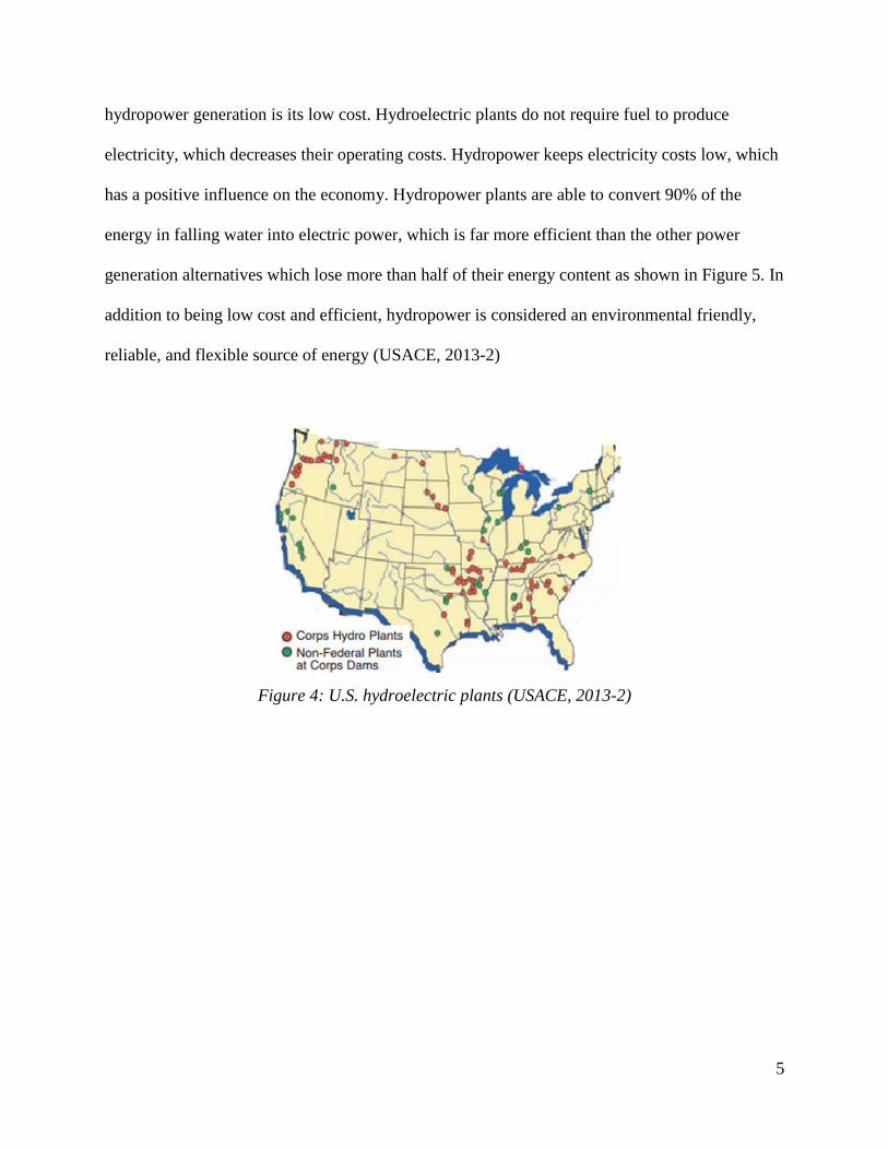
Hydropower is considered the largest source of renewable energy in the U.S., supplying

approximately 52% of the total renewable energy and 6% of the electricity to the nation. As of

2010, 257 billion kilowatt-hours were produced by hydroelectric sources (U.S. Energy

Information Administration, 2011). Figure 4 is a map of the geographical distribution of the

hydropower plants across the United States (USACE, 2013-2). The USACE is considered the

largest operator of hydroelectric plants with a total production of 68 billion kilowatt-hours per

year, which is enough energy to serve approximately 10 million households. One key benefit of

5

hydropower generation is its low cost. Hydroelectric plants do not require fuel to produce

electricity, which decreases their operating costs. Hydropower keeps electricity costs low, which

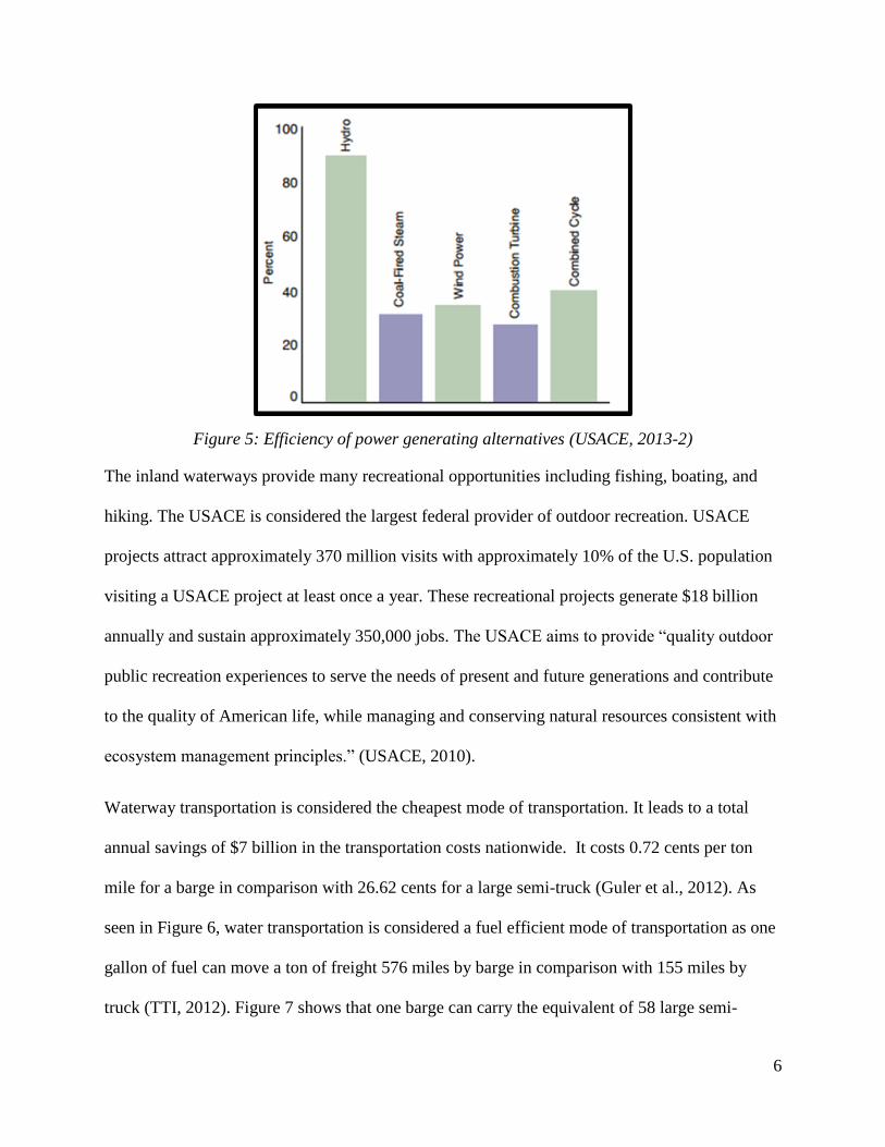
has a positive influence on the economy. Hydropower plants are able to convert 90% of the

energy in falling water into electric power, which is far more efficient than the other power

generation alternatives which lose more than half of their energy content as shown in Figure 5. In

addition to being low cost and efficient, hydropower is considered an environmental friendly,

reliable, and flexible source of energy (USACE, 2013-2)

Figure 4: U.S. hydroelectric plants (USACE, 2013-2)

6

Figure 5: Efficiency of power generating alternatives (USACE, 2013-2)

The inland waterways provide many recreational opportunities including fishing, boating, and

hiking. The USACE is considered the largest federal provider of outdoor recreation. USACE

projects attract approximately 370 million visits with approximately 10% of the U.S. population

visiting a USACE project at least once a year. These recreational projects generate $18 billion

annually and sustain approximately 350,000 jobs. The USACE aims to provide “quality outdoor

public recreation experiences to serve the needs of present and future generations and contribute

to the quality of American life, while managing and conserving natural resources consistent with

ecosystem management principles.” (USACE, 2010).

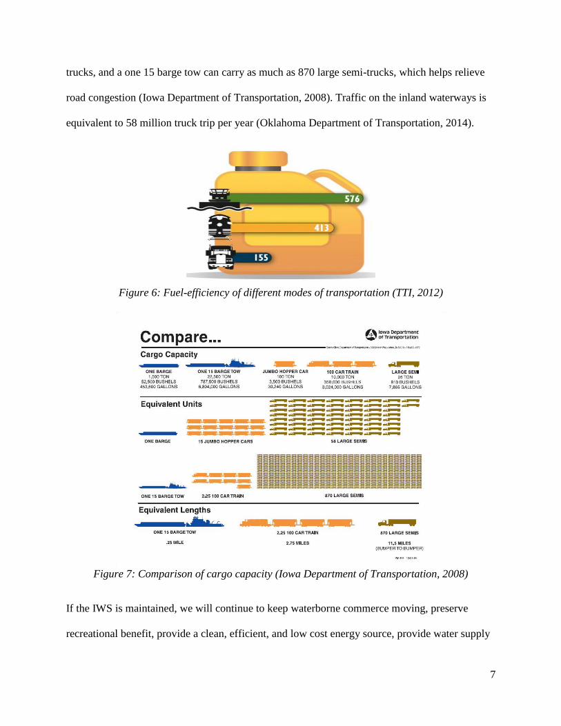
Waterway transportation is considered the cheapest mode of transportation. It leads to a total

annual savings of $7 billion in the transportation costs nationwide. It costs 0.72 cents per ton

mile for a barge in comparison with 26.62 cents for a large semi-truck (Guler et al., 2012). As

seen in Figure 6, water transportation is considered a fuel efficient mode of transportation as one

gallon of fuel can move a ton of freight 576 miles by barge in comparison with 155 miles by

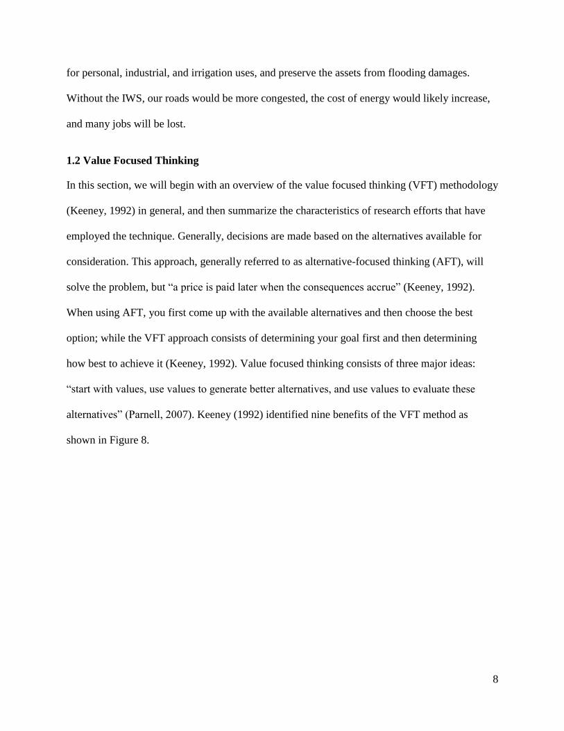
truck (TTI, 2012). Figure 7 shows that one barge can carry the equivalent of 58 large semi-

7

trucks, and a one 15 barge tow can carry as much as 870 large semi-trucks, which helps relieve

road congestion (Iowa Department of Transportation, 2008). Traffic on the inland waterways is

equivalent to 58 million truck trip per year (Oklahoma Department of Transportation, 2014).

Figure 6: Fuel-efficiency of different modes of transportation (TTI, 2012)

Figure 7: Comparison of cargo capacity (Iowa Department of Transportation, 2008)

If the IWS is maintained, we will continue to keep waterborne commerce moving, preserve

recreational benefit, provide a clean, efficient, and low cost energy source, provide water supply

8

for personal, industrial, and irrigation uses, and preserve the assets from flooding damages.

Without the IWS, our roads would be more congested, the cost of energy would likely increase,

and many jobs will be lost.

1.2 Value Focused Thinking

In this section, we will begin with an overview of the value focused thinking (VFT) methodology

(Keeney, 1992) in general, and then summarize the characteristics of research efforts that have

employed the technique. Generally, decisions are made based on the alternatives available for

consideration. This approach, generally referred to as alternative-focused thinking (AFT), will

solve the problem, but “a price is paid later when the consequences accrue” (Keeney, 1992).

When using AFT, you first come up with the available alternatives and then choose the best

option; while the VFT approach consists of determining your goal first and then determining

how best to achieve it (Keeney, 1992). Value focused thinking consists of three major ideas:

“start with values, use values to generate better alternatives, and use values to evaluate these

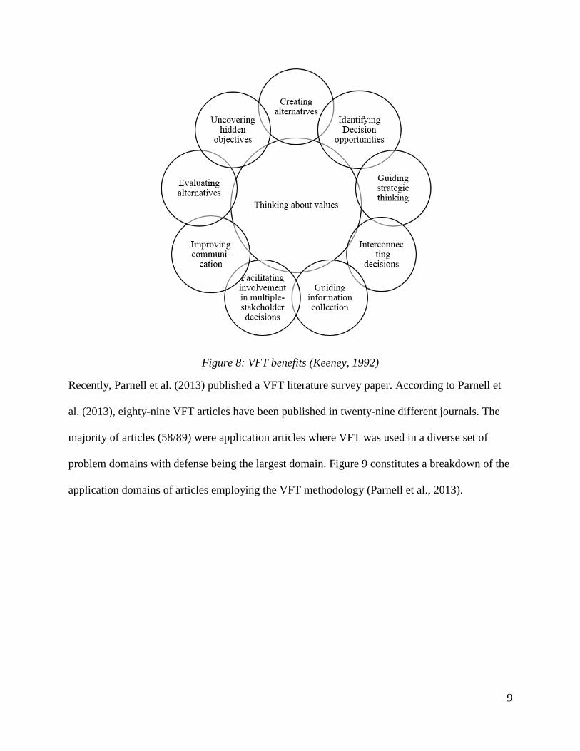
alternatives” (Parnell, 2007). Keeney (1992) identified nine benefits of the VFT method as

shown in Figure 8.

9

Figure 8: VFT benefits (Keeney, 1992)

Recently, Parnell et al. (2013) published a VFT literature survey paper. According to Parnell et

al. (2013), eighty-nine VFT articles have been published in twenty-nine different journals. The

majority of articles (58/89) were application articles where VFT was used in a diverse set of

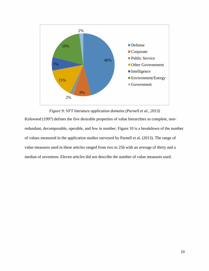
problem domains with defense being the largest domain. Figure 9 constitutes a breakdown of the

application domains of articles employing the VFT methodology (Parnell et al., 2013).

10

Figure 9: VFT literature application domains (Parnell et al., 2013)

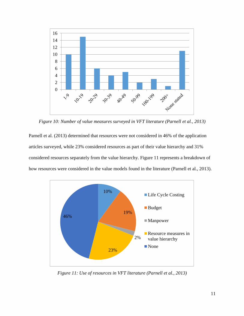
Kirkwood (1997) defines the five desirable properties of value hierarchies as complete, non-

redundant, decomposable, operable, and few in number. Figure 10 is a breakdown of the number

of values measured in the application studies surveyed by Parnell et al. (2013). The range of

value measures used in these articles ranged from two to 256 with an average of thirty and a

median of seventeen. Eleven articles did not describe the number of value measures used.

46%

9%

2%

15%

7%

19%

2%

Defense

Corporate

Public Service

Other Governement

Intelligence

Environment/Energy

Government

11

Figure 10: Number of value measures surveyed in VFT literature (Parnell et al., 2013)

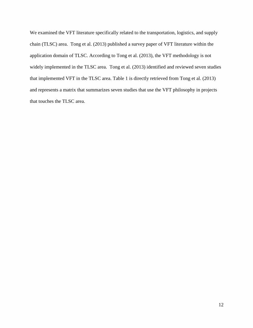
Parnell et al. (2013) determined that resources were not considered in 46% of the application

articles surveyed, while 23% considered resources as part of their value hierarchy and 31%

considered resources separately from the value hierarchy. Figure 11 represents a breakdown of

how resources were considered in the value models found in the literature (Parnell et al., 2013).

Figure 11: Use of resources in VFT literature (Parnell et al., 2013)

0

2

4

6

8

10

12

14

16

10%

19%

2%

23%

46%

Life Cycle Costing

Budget

Manpower

Resource measures in

value hierarchy

None

12

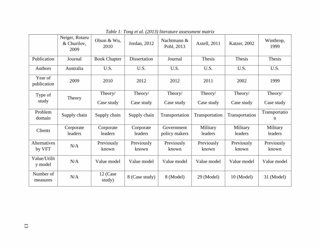
We examined the VFT literature specifically related to the transportation, logistics, and supply

chain (TLSC) area. Tong et al. (2013) published a survey paper of VFT literature within the

application domain of TLSC. According to Tong et al. (2013), the VFT methodology is not

widely implemented in the TLSC area. Tong et al. (2013) identified and reviewed seven studies

that implemented VFT in the TLSC area. Table 1 is directly retrieved from Tong et al. (2013)

and represents a matrix that summarizes seven studies that use the VFT philosophy in projects

that touches the TLSC area.

13

Table 1: Tong et al. (2013) literature assessment matrix

Neiger, Rotaru

& Churilov,

2009

Olson & Wu,

2010 Jordan, 2012

Nachtmann &

Pohl, 2013 Axtell, 2011 Katzer, 2002

Winthrop,

1999

Publication Journal Book Chapter Dissertation Journal Thesis Thesis Thesis

Authors Australia U.S. U.S. U.S. U.S. U.S. U.S.

Year of

publication 2009 2010 2012 2012 2011 2002 1999

Type of

study Theory

Theory/

Case study

Theory/

Case study

Theory/

Case study

Theory/

Case study

Theory/

Case study

Theory/

Case study

Problem

domain Supply chain Supply chain Supply chain Transportation Transportation Transportation

Transportatio

n

Clients Corporate

leaders

Corporate

leaders

Corporate

leaders

Government

policy makers

Military

leaders

Military

leaders

Military

leaders

Alternatives

by VFT N/A

Previously

known

Previously

known

Previously

known

Previously

known

Previously

known

Previously

known

Value/Utilit

y model N/A Value model Value model Value model Value model Value model Value model

Number of

measures N/A

12 (Case

study) 8 (Case study) 8 (Model) 29 (Model) 10 (Model) 31 (Model)

14

1.3 Research Motivation

A preliminary report states that “a wide range of consumers benefit from the pools of water

created and operated to facilitate commercial navigation and other uses, but commercial

navigation itself appears to be a relatively small beneficiary of this system” (U.S. Government

Accountability Office, 2011). Water navigation is an important factor in determining the value of

the IWS; however, a failure of the inland waterways will impact more people than anticipated

when the transportation system was originally conceived. Nachtmann (2007) argues that the

value of inland waterways should be evaluated based on additional factors such as flood

protection, water supply, recreation and tourism, and hydropower generation. Sudar (2005)

argues that while economic measures are important, nontraditional benefits should be taken into

consideration when evaluating the performance of an inland waterway and when making

investment decisions to improve the system. While some tangible benefits are easily associated

with economic value, other more intangible benefits are not.

In general, when making an investment, we should aim for the ‘biggest bang for the buck.’

However, due to the fact that IWS investment benefits are not limited to its transportation

impacts but should also consider other social and environmental benefits, it is difficult to

quantify the total value of these investment decisions. Quantifying the total value of the

investment will depend on what the decision maker values. While an environmentalist may place

more value on environmental benefits, an economist will likely care more about the economic

value of the investment. One of the challenges associated with this method is how to measure

non-traditional benefits (Walker, 2007). The challenge is how to quantify the value of an inland

waterway investment alternative while considering relevant ancillary benefits.

15

1.4 Research Objective

When investing in inland waterway infrastructure, we should aim to maximize all benefits

associated with the investment. The ancillary benefits along with the transportation benefits

associated with the IWS are the focus of our IWS infrastructure investment decision. We

formulate an initial qualitative value model for the inland waterway infrastructure investment

decision utilizing the initial stage in the VFT philosophy (Keeney, 1992). This value model

contains the values that the decision maker cares about when investing in inland waterway

infrastructure. Creating a value hierarchy for the IWS infrastructure investment decision allows

us to holistically evaluate investment alternatives while considering transportation and ancillary

benefits. Given the fact that decision makers have limited resources to invest in inland waterway

infrastructure, a portfolio optimization model (Salo et al., 2011) is formulated to maximize the

overall value associated with inland waterway infrastructure investments while taking in

consideration the budgetary constraints and the minimum desirable value measures outcome

constraints.

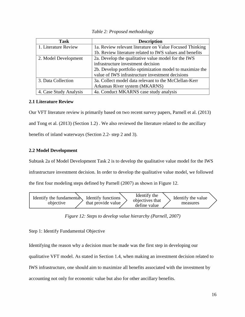
2. Methodology

The methodology used this research is summarized in Table 2, which outlines the tasks that were

completed in order to achieve our research objective.

16

Table 2: Proposed methodology

Task Description

1. Literature Review 1a. Review relevant literature on Value Focused Thinking

1b. Review literature related to IWS values and benefits

2. Model Development 2a. Develop the qualitative value model for the IWS

infrastructure investment decision

2b. Develop portfolio optimization model to maximize the

value of IWS infrastructure investment decisions

3. Data Collection 3a. Collect model data relevant to the McClellan-Kerr

Arkansas River system (MKARNS)

4. Case Study Analysis 4a. Conduct MKARNS case study analysis

2.1 Literature Review

Our VFT literature review is primarily based on two recent survey papers, Parnell et al. (2013)

and Tong et al. (2013) (Section 1.2) . We also reviewed the literature related to the ancillary

benefits of inland waterways (Section 2.2- step 2 and 3).

2.2 Model Development

Subtask 2a of Model Development Task 2 is to develop the qualitative value model for the IWS

infrastructure investment decision. In order to develop the qualitative value model, we followed

the first four modeling steps defined by Parnell (2007) as shown in Figure 12.

Figure 12: Steps to develop value hierarchy (Parnell, 2007)

Step 1: Identify Fundamental Objective

Identifying the reason why a decision must be made was the first step in developing our

qualitative VFT model. As stated in Section 1.4, when making an investment decision related to

IWS infrastructure, one should aim to maximize all benefits associated with the investment by

accounting not only for economic value but also for other ancillary benefits.

Identify the fundamental objective

Identify functions that provide value

Identify the objectives that define value

Identify the value measures

17

Steps 2 and 3: Identify Functions and Objectives

Parnell (2007) states that we can identify the functions that provide value from gold standard

sources (existing documents) or develop them using functional analysis. In order to determine

the functions, a diagram (see Figure 14) was developed to identify the functions and objectives

that provide value. While brainstorming and organizing our gold standard data, a certain amount

of redundancy was generated, but Keeney (1992) states that it is easier to recognize redundant

values if they are explicitly listed than identify the missing ones.

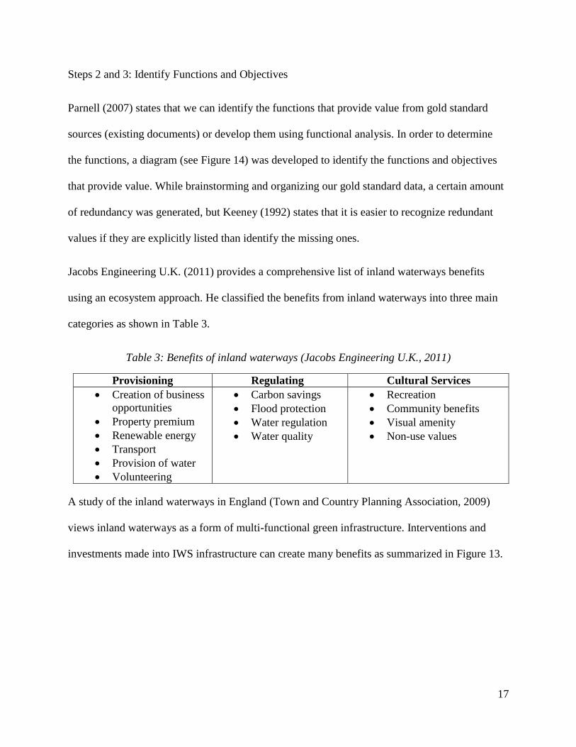
Jacobs Engineering U.K. (2011) provides a comprehensive list of inland waterways benefits

using an ecosystem approach. He classified the benefits from inland waterways into three main

categories as shown in Table 3.

Table 3: Benefits of inland waterways (Jacobs Engineering U.K., 2011)

Provisioning Regulating Cultural Services

Creation of business

opportunities

Property premium

Renewable energy

Transport

Provision of water

Volunteering

Carbon savings

Flood protection

Water regulation

Water quality

Recreation

Community benefits

Visual amenity

Non-use values

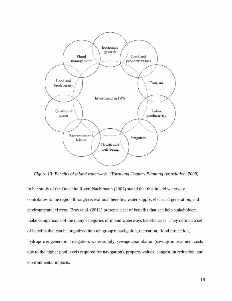
A study of the inland waterways in England (Town and Country Planning Association, 2009)

views inland waterways as a form of multi-functional green infrastructure. Interventions and

investments made into IWS infrastructure can create many benefits as summarized in Figure 13.

18

Figure 13: Benefits of inland waterways. (Town and Country Planning Association, 2009)

In her study of the Ouachita River, Nachtmann (2007) stated that this inland waterway

contributes to the region through recreational benefits, water supply, electrical generation, and

environmental effects. Bray et al. (2011) presents a set of benefits that can help stakeholders

make comparisons of the many categories of inland waterways beneficiaries. They defined a set

of benefits that can be organized into ten groups: navigation, recreation, flood protection,

hydropower generation, irrigation, water supply, sewage assimilation (savings in treatment costs

due to the higher pool levels required for navigation), property values, congestion reduction, and

environmental impacts.

19

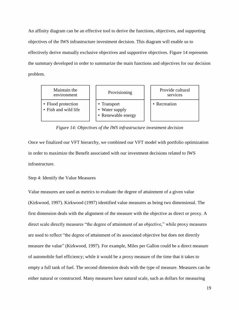
An affinity diagram can be an effective tool to derive the functions, objectives, and supporting

objectives of the IWS infrastructure investment decision. This diagram will enable us to

effectively derive mutually exclusive objectives and supportive objectives. Figure 14 represents

the summary developed in order to summarize the main functions and objectives for our decision

problem.

Figure 14: Objectives of the IWS infrastructure investment decision

Once we finalized our VFT hierarchy, we combined our VFT model with portfolio optimization

in order to maximize the Benefit associated with our investment decisions related to IWS

infrastructure.

Step 4: Identify the Value Measures

Value measures are used as metrics to evaluate the degree of attainment of a given value

(Kirkwood, 1997). Kirkwood (1997) identified value measures as being two dimensional. The

first dimension deals with the alignment of the measure with the objective as direct or proxy. A

direct scale directly measures “the degree of attainment of an objective,” while proxy measures

are used to reflect “the degree of attainment of its associated objective but does not directly

measure the value” (Kirkwood, 1997). For example, Miles per Gallon could be a direct measure

of automobile fuel efficiency; while it would be a proxy measure of the time that it takes to

empty a full tank of fuel. The second dimension deals with the type of measure. Measures can be

either natural or constructed. Many measures have natural scale, such as dollars for measuring

Maintain the environment

• Flood protection

• Fish and wild life

Provisioning

• Transport

• Water supply

• Renewable energy

Provide cultural services

• Recreation

20

cost, but others do not have natural scale such as customer satisfaction. Table 4 represents the

preferences of Parnell (2007) for the types of measures.

Table 4: Types of measures preference Parnell (2007)

Type Direct

Alignment

Proxy

Alignment

Natural 1 3

Constructed 2 4

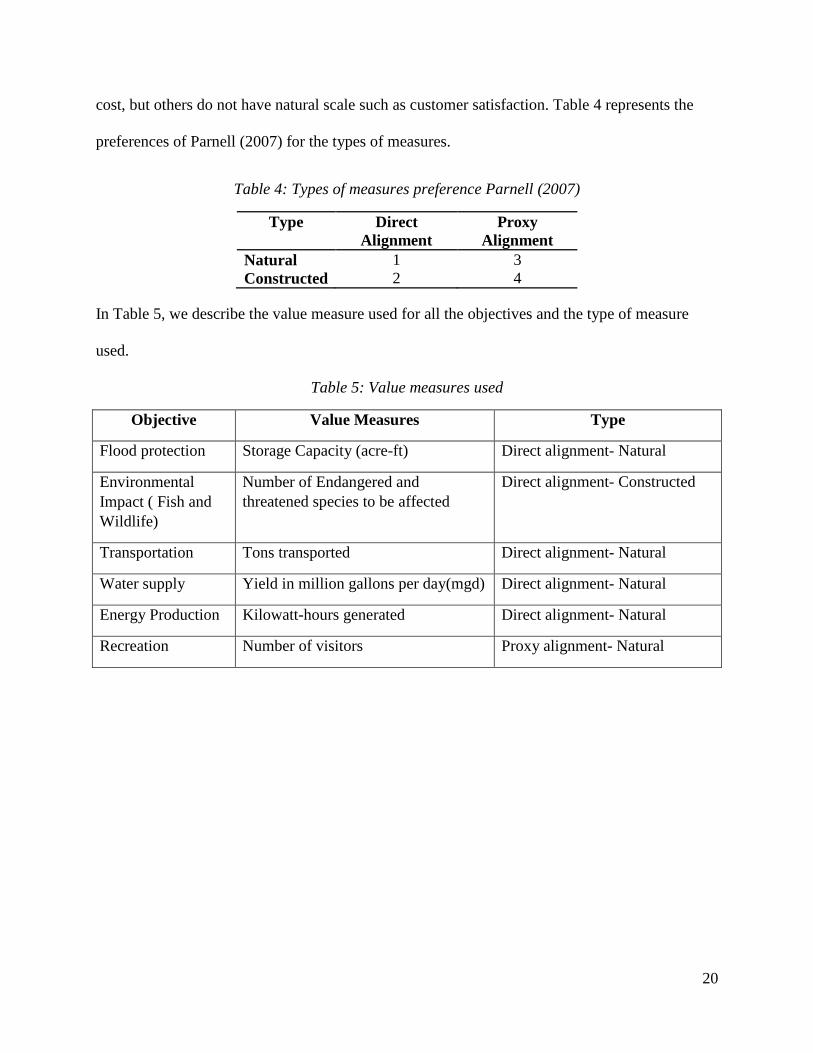
In Table 5, we describe the value measure used for all the objectives and the type of measure

used.

Table 5: Value measures used

Objective Value Measures Type

Flood protection Storage Capacity (acre-ft) Direct alignment- Natural

Environmental

Impact ( Fish and

Wildlife)

Number of Endangered and

threatened species to be affected

Direct alignment- Constructed

Transportation Tons transported Direct alignment- Natural

Water supply Yield in million gallons per day(mgd) Direct alignment- Natural

Energy Production Kilowatt-hours generated Direct alignment- Natural

Recreation Number of visitors Proxy alignment- Natural

21

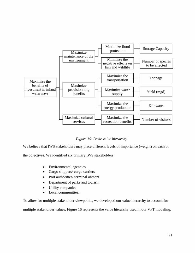
Figure 15: Basic value hierarchy

We believe that IWS stakeholders may place different levels of importance (weight) on each of

the objectives. We identified six primary IWS stakeholders:

Environmental agencies

Cargo shippers/ cargo carriers

Port authorities/ terminal owners

Department of parks and tourism

Utility companies

Local communities.

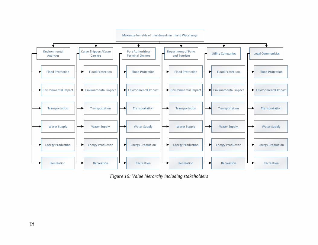
To allow for multiple stakeholder viewpoints, we developed our value hierarchy to account for

multiple stakeholder values. Figure 16 represents the value hierarchy used in our VFT modeling.

Maximize the benefits of

investment in inland waterways

Maximize maintenance of the

environment

Maximize flood protection

Storage Capacity

Minimize the negative effects on fish and wildlife

Number of species to be affected

Maximize provisionning

benefits

Maximize the transportation

Tonnage

Maximize water supply

Yield (mgd)

Maximize the energy production

Kilowatts

Maximize cultural services

Maximize the recreation benefits

Number of visitors

22

Maximize benefits of Investments in Inland Waterways

Environmental Agencies

Cargo Shippers/Cargo Carriers

Port Authorities/Terminal Owners

Department of Parks and Tourism

Utility Companies Local Communities

Flood Protection Flood Protection Flood Protection Flood Protection Flood Protection Flood Protection

Environmental Impact Environmental Impact Environmental Impact Environmental Impact Environmental Impact Environmental Impact

Transportation Transportation Transportation Transportation Transportation Transportation

Water Supply Water Supply Water Supply Water Supply Water Supply Water Supply

Energy Production Energy Production Energy Production Energy Production Energy Production Energy Production

Recreation Recreation Recreation Recreation Recreation Recreation

Figure 16: Value hierarchy including stakeholders

23

3. Case Study Development

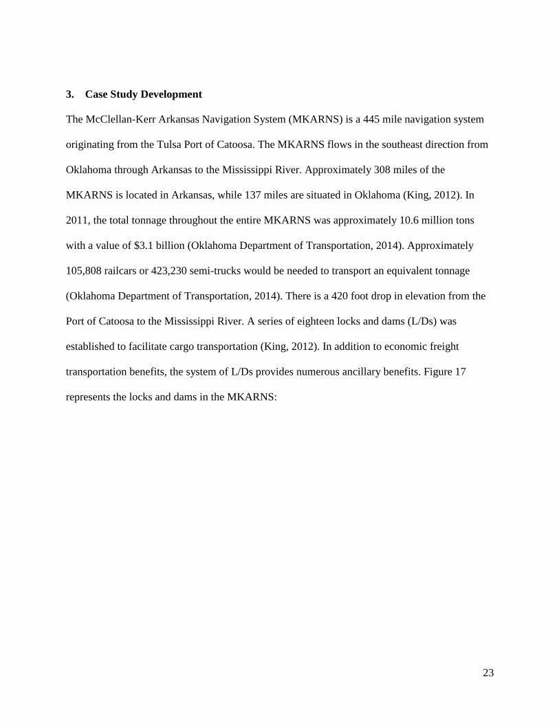
The McClellan-Kerr Arkansas Navigation System (MKARNS) is a 445 mile navigation system

originating from the Tulsa Port of Catoosa. The MKARNS flows in the southeast direction from

Oklahoma through Arkansas to the Mississippi River. Approximately 308 miles of the

MKARNS is located in Arkansas, while 137 miles are situated in Oklahoma (King, 2012). In

2011, the total tonnage throughout the entire MKARNS was approximately 10.6 million tons

with a value of $3.1 billion (Oklahoma Department of Transportation, 2014). Approximately

105,808 railcars or 423,230 semi-trucks would be needed to transport an equivalent tonnage

(Oklahoma Department of Transportation, 2014). There is a 420 foot drop in elevation from the

Port of Catoosa to the Mississippi River. A series of eighteen locks and dams (L/Ds) was

established to facilitate cargo transportation (King, 2012). In addition to economic freight

transportation benefits, the system of L/Ds provides numerous ancillary benefits. Figure 17

represents the locks and dams in the MKARNS:

24

Figure 17: MKARNS lock lift (King, 2012)

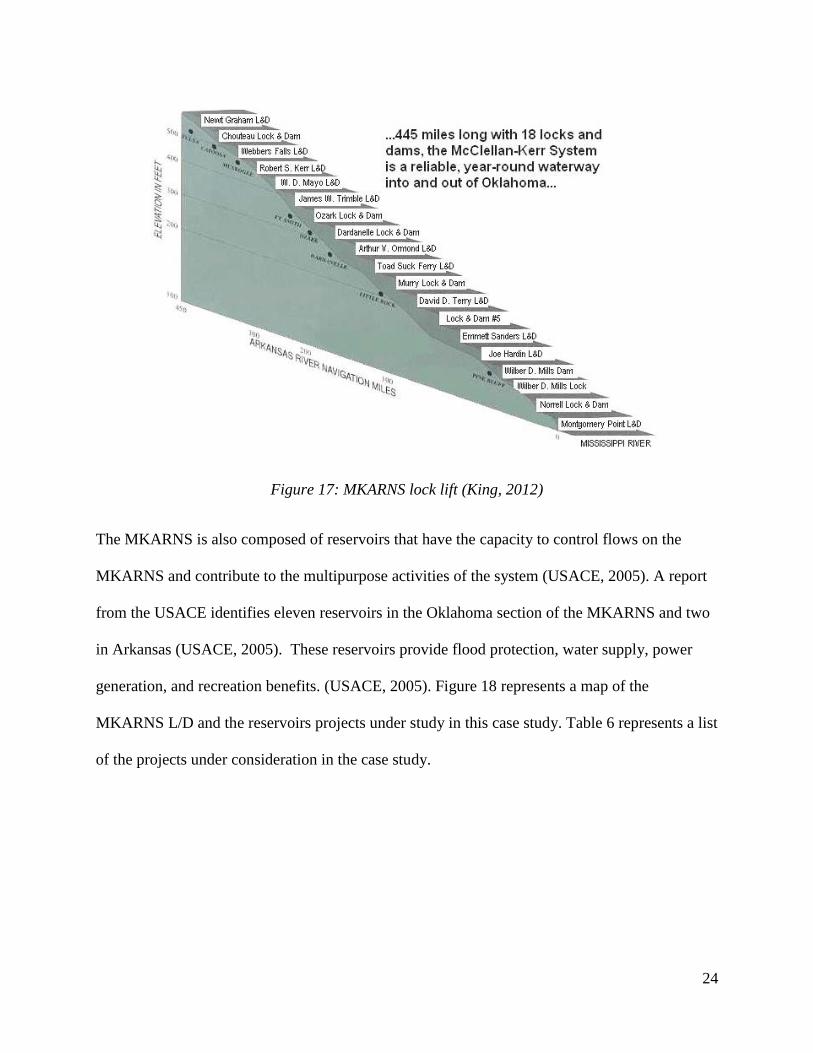
The MKARNS is also composed of reservoirs that have the capacity to control flows on the

MKARNS and contribute to the multipurpose activities of the system (USACE, 2005). A report

from the USACE identifies eleven reservoirs in the Oklahoma section of the MKARNS and two

in Arkansas (USACE, 2005). These reservoirs provide flood protection, water supply, power

generation, and recreation benefits. (USACE, 2005). Figure 18 represents a map of the

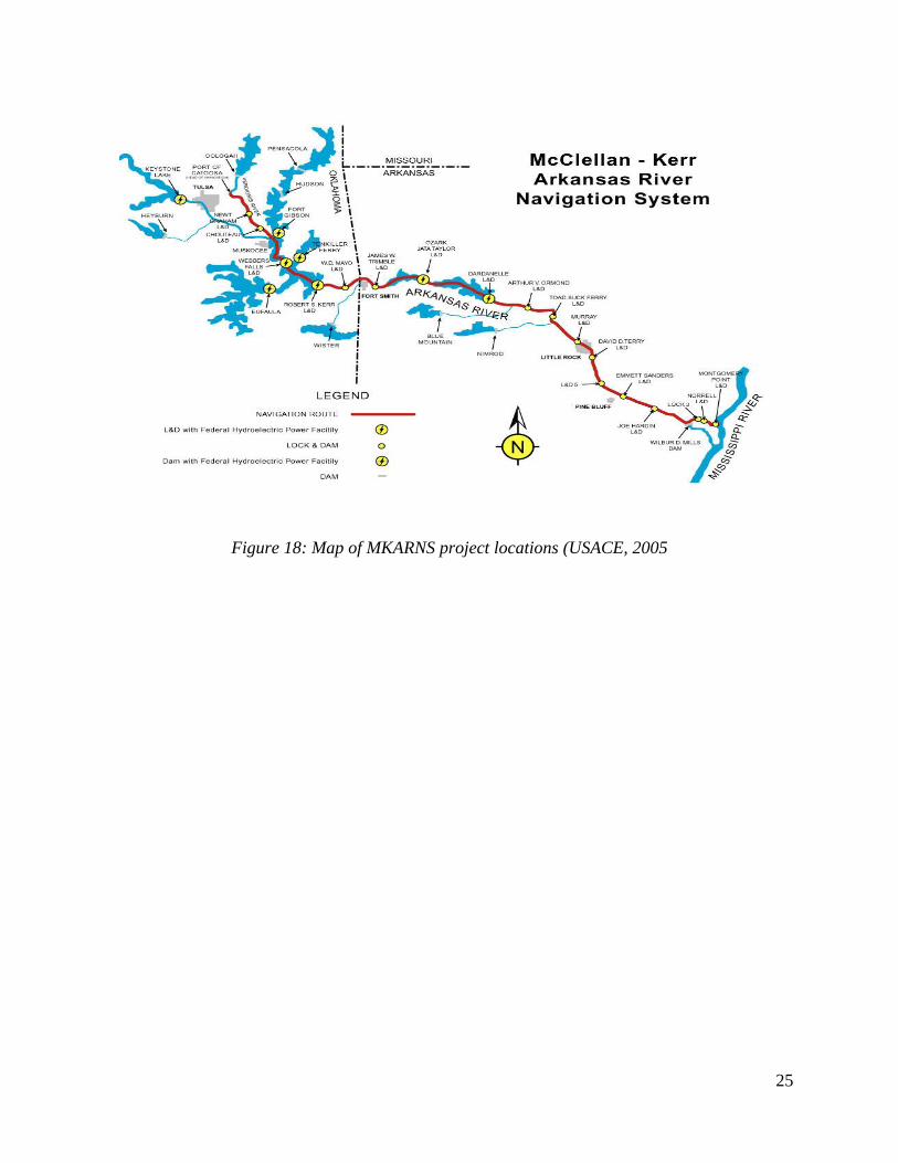
MKARNS L/D and the reservoirs projects under study in this case study. Table 6 represents a list

of the projects under consideration in the case study.

25

Figure 18: Map of MKARNS project locations (USACE, 2005

26

Table 6: List of case study projects, type, and state location

State MKARNS Project Type of Project

Ark

ansas

Norrell L&D L/D

Arkansas L&D 2 L/D

Emmett Sanders L&D L/D

Joe Hardin L&D L/D

Arkansas L&D 5 L/D

David D Terry L&D L/D

Toad Suck Ferry L&D L/D

Murray L&D L/D

Dardanelle L&D L/D

Arthur V Ormond L&D L/D

Ozark-JetaTaylor L&D L/D

James W Trimble L&D L/D

Blue Mountain Reservoir

Nimrod Reservoir

Oklah

om

a

Robert S Kerr L&D L/D

W D Mayo L&D L/D

Webbers Falls L&D L/D

Newt Graham L&D L/D

Chouteau L&D L/D

Keystone Reservoir

Oologah Reservoir

Pensacola Dam Reservoir

Markham Ferry Dam Reservoir

Fort Gibson Reservoir

Tenkiller Ferry Reservoir

Eufaula Reservoir

Kaw Reservoir

Hulah Reservoir

Copan Reservoir

Wister Reservoir

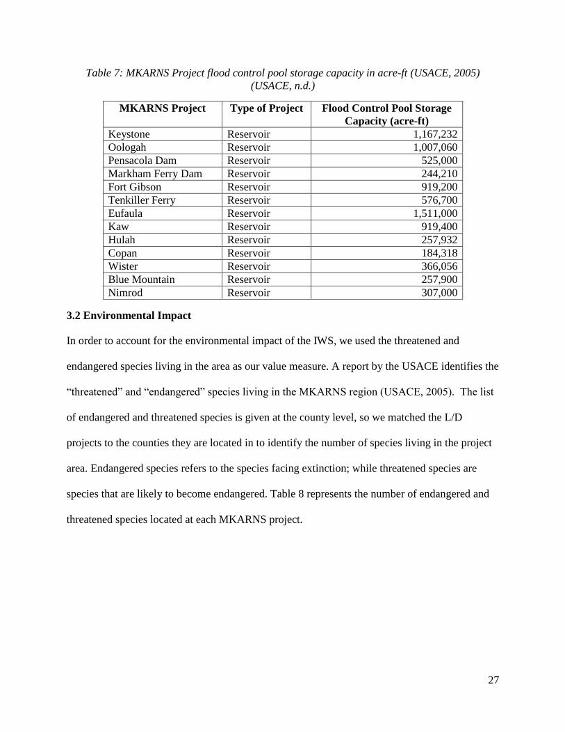
3.1 Flood Protection

The Oklahoma upstream reservoirs and the two Arkansas reservoirs provide flood protection and

water supply benefits. The pools of the MKARNS L/D projects are used to keep the water levels

in the river deep enough for the navigation and are not used for any type of flood protection

(USACE, n.d.). Table 7 provides the flood control pool storage capacities in acre-feet for each

MKARNS project with a flood protection benefit.

27

Table 7: MKARNS Project flood control pool storage capacity in acre-ft (USACE, 2005)

(USACE, n.d.)

MKARNS Project Type of Project Flood Control Pool Storage

Capacity (acre-ft)

Keystone Reservoir 1,167,232

Oologah Reservoir 1,007,060

Pensacola Dam Reservoir 525,000

Markham Ferry Dam Reservoir 244,210

Fort Gibson Reservoir 919,200

Tenkiller Ferry Reservoir 576,700

Eufaula Reservoir 1,511,000

Kaw Reservoir 919,400

Hulah Reservoir 257,932

Copan Reservoir 184,318

Wister Reservoir 366,056

Blue Mountain Reservoir 257,900

Nimrod Reservoir 307,000

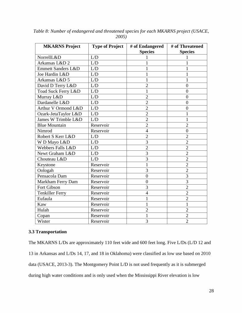
3.2 Environmental Impact

In order to account for the environmental impact of the IWS, we used the threatened and

endangered species living in the area as our value measure. A report by the USACE identifies the

“threatened” and “endangered” species living in the MKARNS region (USACE, 2005). The list

of endangered and threatened species is given at the county level, so we matched the L/D

projects to the counties they are located in to identify the number of species living in the project

area. Endangered species refers to the species facing extinction; while threatened species are

species that are likely to become endangered. Table 8 represents the number of endangered and

threatened species located at each MKARNS project.

28

Table 8: Number of endangered and threatened species for each MKARNS project (USACE,

2005)

MKARNS Project Type of Project # of Endangered

Species

# of Threatened

Species

NorrellL&D L/D 1 1

Arkansas L&D 2 L/D 1 1

Emmett Sanders L&D L/D 1 1

Joe Hardin L&D L/D 1 1

Arkansas L&D 5 L/D 1 1

David D Terry L&D L/D 2 0

Toad Suck Ferry L&D L/D 1 0

Murray L&D L/D 2 0

Dardanelle L&D L/D 2 0

Arthur V Ormond L&D L/D 2 0

Ozark-JetaTaylor L&D L/D 2 1

James W Trimble L&D L/D 2 1

Blue Mountain Reservoir 2 2

Nimrod Reservoir 4 0

Robert S Kerr L&D L/D 2 2

W D Mayo L&D L/D 3 2

Webbers Falls L&D L/D 2 2

Newt Graham L&D L/D 3 2

Chouteau L&D L/D 3 2

Keystone Reservoir 1 2

Oologah Reservoir 3 2

Pensacola Dam Reservoir 0 3

Markham Ferry Dam Reservoir 0 3

Fort Gibson Reservoir 3 2

Tenkiller Ferry Reservoir 4 2

Eufaula Reservoir 1 2

Kaw Reservoir 1 1

Hulah Reservoir 2 2

Copan Reservoir 1 2

Wister Reservoir 3 2

3.3 Transportation

The MKARNS L/Ds are approximately 110 feet wide and 600 feet long. Five L/Ds (L/D 12 and

13 in Arkansas and L/Ds 14, 17, and 18 in Oklahoma) were classified as low use based on 2010

data (USACE, 2013-3). The Montgomery Point L/D is not used frequently as it is submerged

during high water conditions and is only used when the Mississippi River elevation is low

29

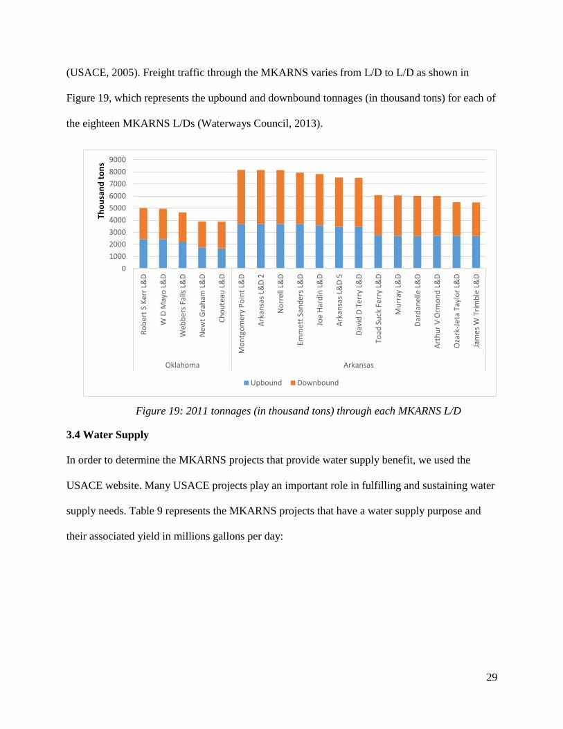
(USACE, 2005). Freight traffic through the MKARNS varies from L/D to L/D as shown in

Figure 19, which represents the upbound and downbound tonnages (in thousand tons) for each of

the eighteen MKARNS L/Ds (Waterways Council, 2013).

Figure 19: 2011 tonnages (in thousand tons) through each MKARNS L/D

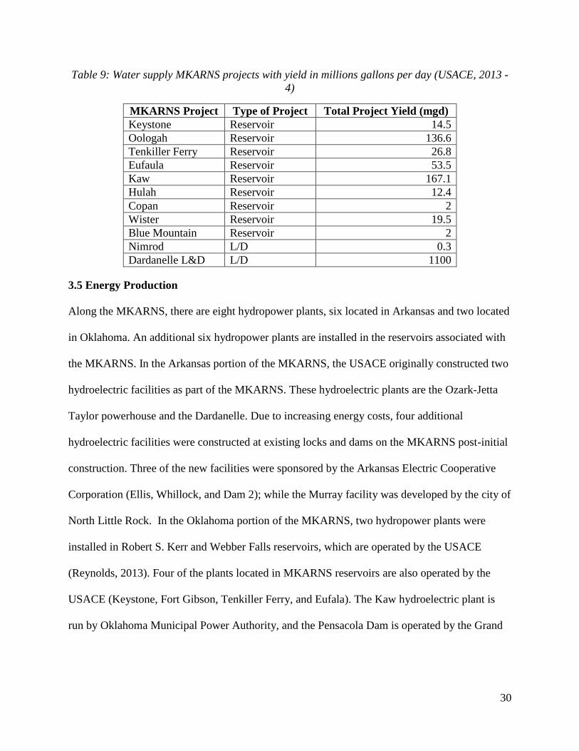
3.4 Water Supply

In order to determine the MKARNS projects that provide water supply benefit, we used the

USACE website. Many USACE projects play an important role in fulfilling and sustaining water

supply needs. Table 9 represents the MKARNS projects that have a water supply purpose and

their associated yield in millions gallons per day:

0

1000

2000

3000

4000

5000

6000

7000

8000

9000

Ro

ber

t S

Ker

r L&

D

W D

May

o L

&D

Web

ber

s Fa

lls L

&D

Ne

wt

Gra

ham

L&

D

Ch

ou

teau

L&

D

Mo

ntg

om

ery

Po

int

L&D

Ark

ansa

s L&

D 2

No

rre

ll L&

D

Emm

ett

San

de

rs L

&D

Joe

Har

din

L&

D

Ark

ansa

s L&

D 5

Dav

id D

Ter

ry L

&D

Toad

Su

ck F

err

y L&

D

Mu

rray

L&

D

Dar

dan

elle

L&

D

Art

hu

r V

Orm

on

d L

&D

Oza

rk-J

eta

Tay

lor

L&D

Jam

es W

Tri

mb

le L

&D

Oklahoma Arkansas

Tho

usa

nd

to

ns

Upbound Downbound

30

Table 9: Water supply MKARNS projects with yield in millions gallons per day (USACE, 2013 -

4)

MKARNS Project Type of Project Total Project Yield (mgd)

Keystone Reservoir 14.5

Oologah Reservoir 136.6

Tenkiller Ferry Reservoir 26.8

Eufaula Reservoir 53.5

Kaw Reservoir 167.1

Hulah Reservoir 12.4

Copan Reservoir 2

Wister Reservoir 19.5

Blue Mountain Reservoir 2

Nimrod L/D 0.3

Dardanelle L&D L/D 1100

3.5 Energy Production

Along the MKARNS, there are eight hydropower plants, six located in Arkansas and two located

in Oklahoma. An additional six hydropower plants are installed in the reservoirs associated with

the MKARNS. In the Arkansas portion of the MKARNS, the USACE originally constructed two

hydroelectric facilities as part of the MKARNS. These hydroelectric plants are the Ozark-Jetta

Taylor powerhouse and the Dardanelle. Due to increasing energy costs, four additional

hydroelectric facilities were constructed at existing locks and dams on the MKARNS post-initial

construction. Three of the new facilities were sponsored by the Arkansas Electric Cooperative

Corporation (Ellis, Whillock, and Dam 2); while the Murray facility was developed by the city of

North Little Rock. In the Oklahoma portion of the MKARNS, two hydropower plants were

installed in Robert S. Kerr and Webber Falls reservoirs, which are operated by the USACE

(Reynolds, 2013). Four of the plants located in MKARNS reservoirs are also operated by the

USACE (Keystone, Fort Gibson, Tenkiller Ferry, and Eufala). The Kaw hydroelectric plant is

run by Oklahoma Municipal Power Authority, and the Pensacola Dam is operated by the Grand

31

River Dam Authority. Table 10 represents the installed capacity (in Kilowatts (KWs)) of each

MKARNS project with hydropower capability.

Table 10: MKARNS Projects with hydropower installed capacity in Kilowatts (USACE, 2005)

MKARNS Project Type of Project Installed Hydropower

Capacity (KWs)

Arkansas L&D 2 L/D 108,000

Murray L&D L/D 39,000

Dardanelle L&D L/D 148,000

Arthur V Ormond L&D L/D 32,400

Ozark-Jeta Taylor L&D L/D 100,000

James W Trimble L&D L/D 32,400

Robert S Kerr L&D L/D 110,000

Webbers Falls L&D L/D 60,000

Keystone Reservoir 70,000


Fort Gibson Reservoir 45,000

Tenkiller Ferry Reservoir 39,100

Eufaula Reservoir 90,000


3.6 Recreation

The MKARNS created important lakes that are considered recreational havens for outdoor

recreation users. Lakes and parks play an important role in the tourism-based economy in

Arkansas. According to USACE (2012-1), the Little Rock Corps of Engineers district is ranked

in the top five Corps districts based on recreational project visitation. In 2011, 3,547 recreational

vessels locked through the thirteen locks on the Arkansas portion of the MKARNS; while 1,134

recreational vessels locked through the Oklahoma locks (King, 2012). Table 11 provides the

USACE estimates of the number of visits to the L/D recreation spots alongside the MKARNS

and the reservoirs associated with the MKARNS.

32

Table 11: MKARNS projects with number of recreational visitors (USACE, 2012-2)

MKARNS Project Type of project # of Recreational

Visitors

Norrell L&D L/D 23,702


Emmett Sanders L&D L/D 256,564

Joe Hardin L&D L/D 38,506


David D Terry L&D L/D 1,256,852

Toad Suck Ferry L&D L/D 146,983

Murray L&D L/D 461,504

Dardanelle L&D L/D 1,304,569

Arthur V Ormond L&D L/D 74,187

Ozark-JetaTaylor L&D L/D 519,159

James W Trimble L&D L/D 473,808

Blue Mountain Reservoir 405,025

Nimrod Reservoir 226,048

Robert S Kerr L&D L/D 271,719

W D Mayo L&D L/D 48,921

Webbers Falls L&D L/D 663,913

Newt Graham L&D L/D 123,019

Chouteau L&D L/D 95,036

Keystone Reservoir 1,062,635

Oologah Reservoir 894,978


Markham Ferry Dam Reservoir 167,467

Fort Gibson Reservoir 1,677,535

Tenkiller Ferry Reservoir 2,583,915

Eufaula Reservoir 2,466,286


Hulah Reservoir 59,350

Copan Reservoir 52,311

Wister Reservoir 205,815

4. Model Development

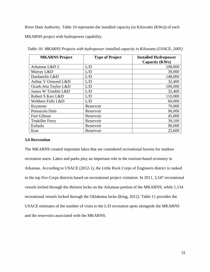
4.1 Development of the Value Functions

The value functions measure the returns to scale of the value measures. According to Parnell

(2007), the value functions can take on four shapes: linear, convex, concave, and S-curve. In our

study, we assume that each increment of the measure is equally valuable for flood protection,

33

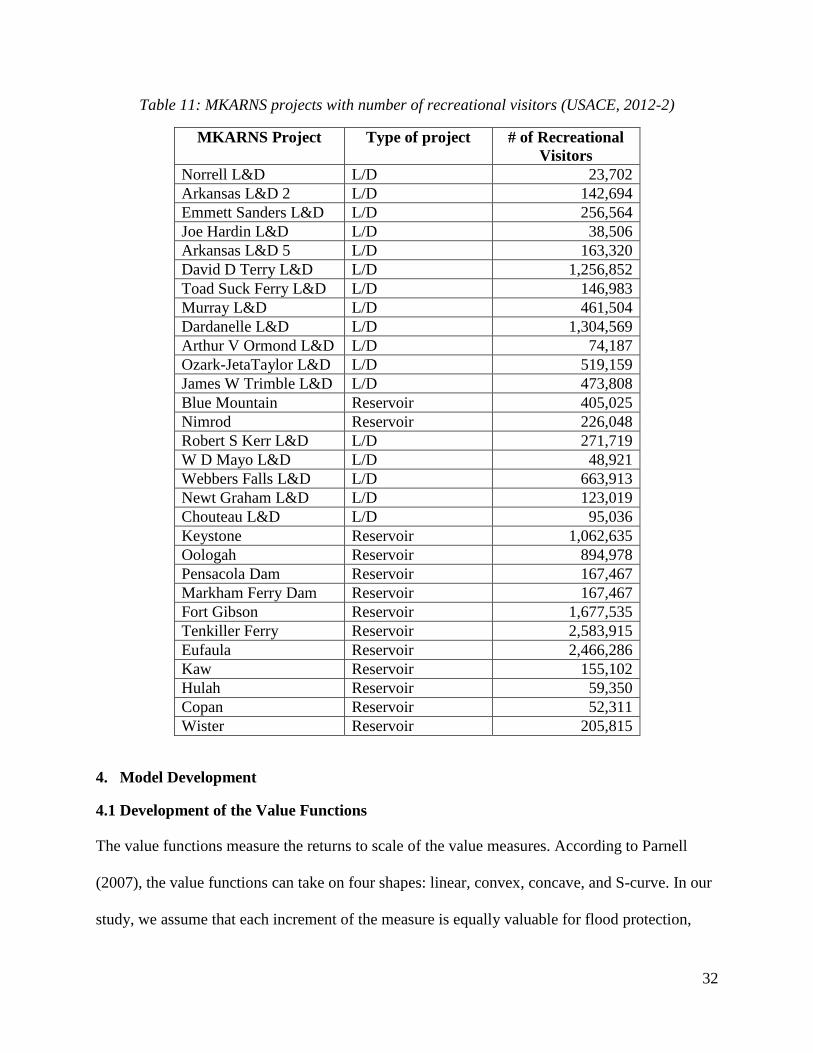
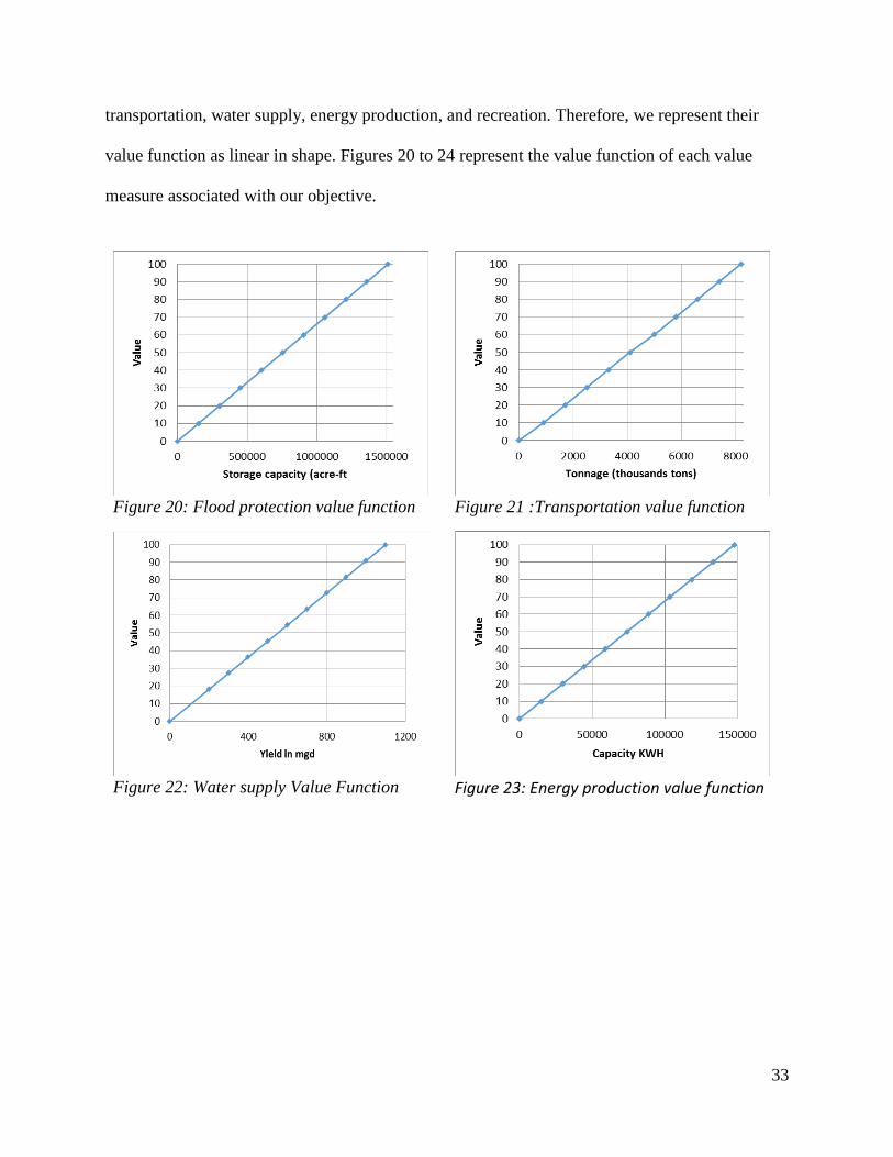
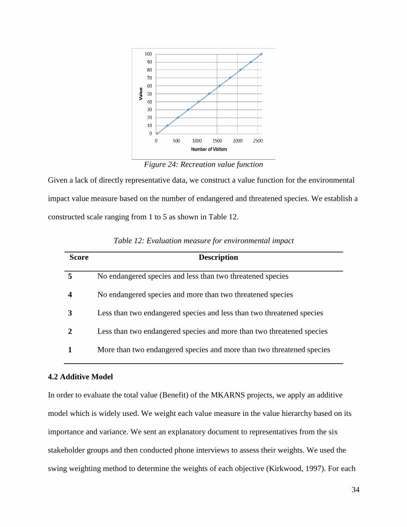
transportation, water supply, energy production, and recreation. Therefore, we represent their

value function as linear in shape. Figures 20 to 24 represent the value function of each value

measure associated with our objective.

Figure 20: Flood protection value function

Figure 21 :Transportation value function

Figure 22: Water supply Value Function

Figure 23: Energy production value function

34

Given a lack of directly representative data, we construct a value function for the environmental

impact value measure based on the number of endangered and threatened species. We establish a

constructed scale ranging from 1 to 5 as shown in Table 12.

Table 12: Evaluation measure for environmental impact

Score Description

5 No endangered species and less than two threatened species

4 No endangered species and more than two threatened species

3 Less than two endangered species and less than two threatened species

2 Less than two endangered species and more than two threatened species

1 More than two endangered species and more than two threatened species

4.2 Additive Model

In order to evaluate the total value (Benefit) of the MKARNS projects, we apply an additive

model which is widely used. We weight each value measure in the value hierarchy based on its

importance and variance. We sent an explanatory document to representatives from the six

stakeholder groups and then conducted phone interviews to assess their weights. We used the

swing weighting method to determine the weights of each objective (Kirkwood, 1997). For each

Figure 24: Recreation value function

35

stakeholder, the weights are normalized to sum to 1(equation 2). Let αj be represents the

importance of each of the stakeholder weight, wji the weight for objective i for stakeholder j, and

υ(xi) is the single dimensional value function that converts the evaluation measure to a common

value scale (Parnell, 2005) represented by Figures 20 to 24. The value function υ(αj, xi) allows us

to score the alternatives and is defined by Equation (1).

V(αj, 𝑥i) = ∑ ∑ α𝑗

𝑖𝑗

w𝑗𝑖 υ(𝑥𝑖) (1)

Such as

∑ 𝑤𝑗𝑖 = 1 ∀𝑗 ∈ 𝑠𝑡𝑎𝑘𝑒ℎ𝑜𝑙𝑑𝑒𝑟𝑠

𝑖

(2)

∑ α𝑗 = 1

𝑗

(3)

In order to obtain the weights for each stakeholder group, we attempted to conduct phone

interviews with at least one representative of each group. Each stakeholder was asked to provide

an assessment 𝑓𝑖𝑗of the importance of each objective i between 0 and 10, while taking in

consideration the ranges attainable on each objective (Kirkwood, 1997). After the assessments

𝑓𝑖𝑗 were collected or assumed for all objectives i for each stakeholder j, the weights were

normalized so that their sum is equal to 1 for each stakeholder j, by using Equation (4):

𝑤𝑗𝑖 = 𝑓𝑖𝑗

∑ 𝑓𝑖𝑗𝑖 ∀𝑗 ∈ 𝑠𝑡𝑎𝑘𝑒ℎ𝑜𝑙𝑑𝑒𝑟 (4)

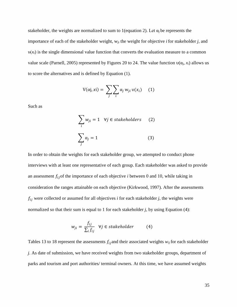
Tables 13 to 18 represent the assessments 𝑓𝑖𝑗and their associated weights wij for each stakeholder

j. As date of submission, we have received weights from two stakeholder groups, department of

parks and tourism and port authorities/ terminal owners. At this time, we have assumed weights

36

for the other four stakeholder groups and are continuing to contact these stakeholders. We plan to

rerun the analysis once additional expert assessments are received.

Table 13: Values assessments and weights for environmental agencies

Values Assessment 𝒇𝒊𝒋 Weight wij

Flood protection 8 21.05%

Environmental impact 10 26.32%

Transportation 3 7.89%

Water supply 7 18.42%

Energy production 5 13.16%

Recreation 5 13.16%

Table 14: Values assessments and weights for cargo shippers/cargo carriers







Recreation 1 2.94%

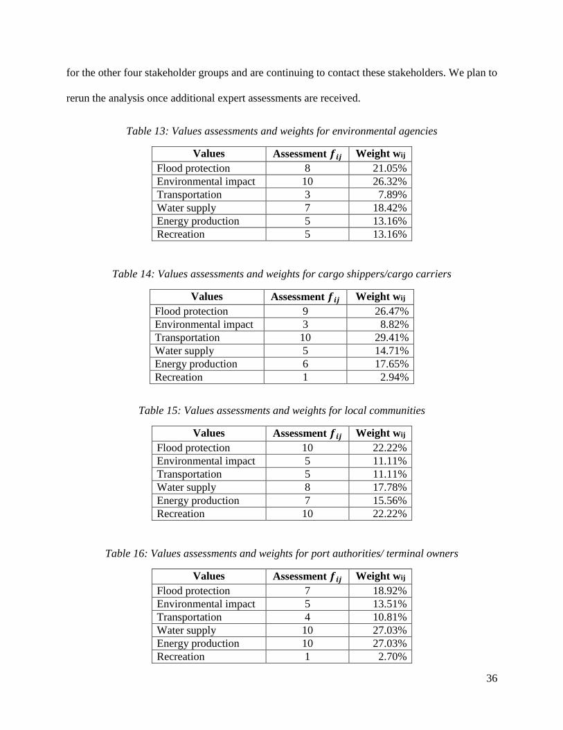
Table 15: Values assessments and weights for local communities







Recreation 10 22.22%

Table 16: Values assessments and weights for port authorities/ terminal owners







Recreation 1 2.70%

37

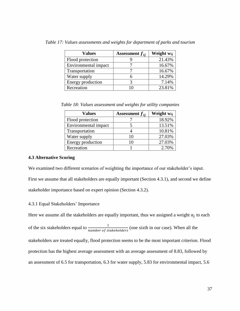
Table 17: Values assessments and weights for department of parks and tourism







Recreation 10 23.81%

Table 18: Values assessment and weights for utility companies







Recreation 1 2.70%

4.3 Alternative Scoring

We examined two different scenarios of weighting the importance of our stakeholder’s input.

First we assume that all stakeholders are equally important (Section 4.3.1), and second we define

stakeholder importance based on expert opinion (Section 4.3.2).

4.3.1 Equal Stakeholders’ Importance

Here we assume all the stakeholders are equally important, thus we assigned a weight α𝑗 to each

of the six stakeholders equal to 1

𝑛𝑢𝑚𝑏𝑒𝑟 𝑜𝑓 𝑠𝑡𝑎𝑘𝑒ℎ𝑜𝑙𝑑𝑒𝑟𝑠 (one sixth in our case). When all the

stakeholders are treated equally, flood protection seems to be the most important criterion. Flood

protection has the highest average assessment with an average assessment of 8.83, followed by

an assessment of 6.5 for transportation, 6.3 for water supply, 5.83 for environmental impact, 5.6

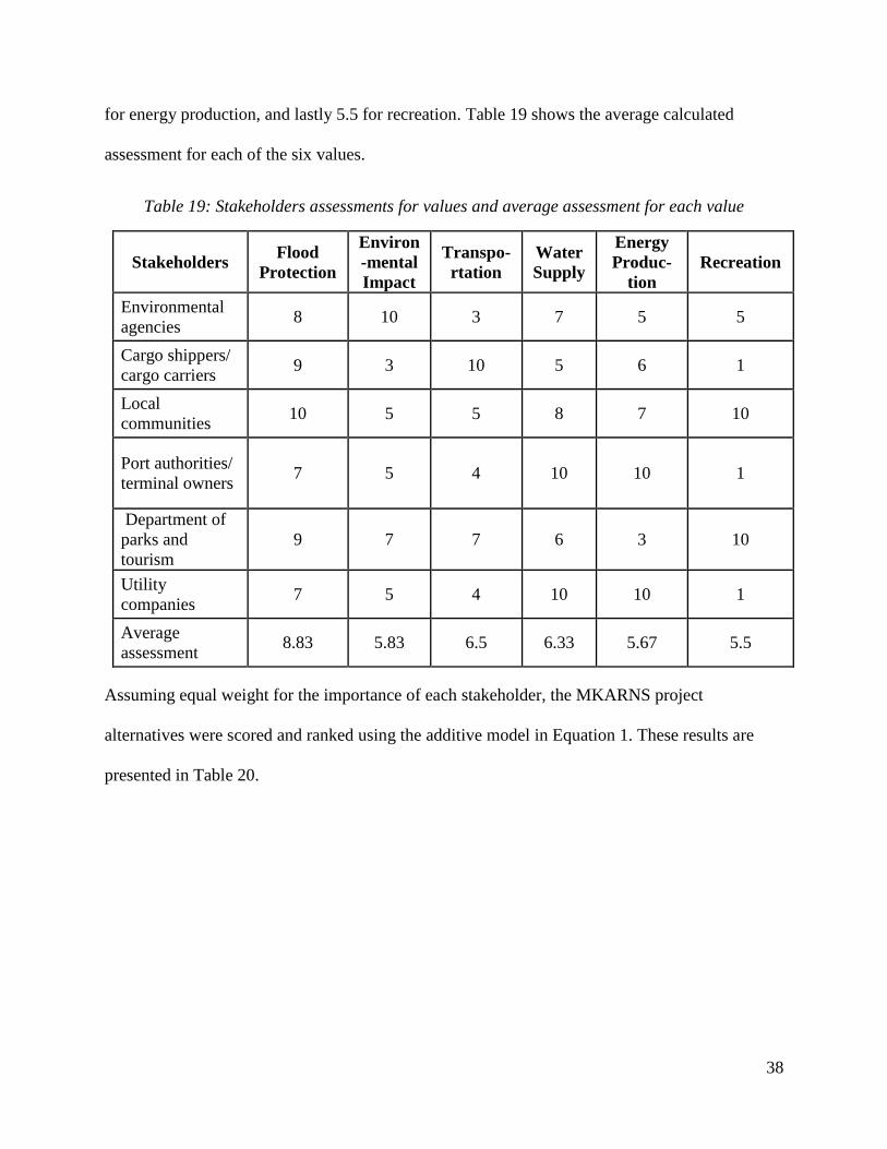
38

for energy production, and lastly 5.5 for recreation. Table 19 shows the average calculated

assessment for each of the six values.

Table 19: Stakeholders assessments for values and average assessment for each value

Stakeholders Flood

Protection

Environ

-mental

Impact

Transpo-

rtation

Water

Supply

Energy

Produc-

tion

Recreation

Environmental

agencies 8 10 3 7 5 5

Cargo shippers/

cargo carriers 9 3 10 5 6 1

Local

communities 10 5 5 8 7 10

Port authorities/

terminal owners 7 5 4 10 10 1

Department of

parks and

tourism

9 7 7 6 3 10

Utility

companies 7 5 4 10 10 1

Average

assessment 8.83 5.83 6.5 6.33 5.67 5.5

Assuming equal weight for the importance of each stakeholder, the MKARNS project

alternatives were scored and ranked using the additive model in Equation 1. These results are

presented in Table 20.

39

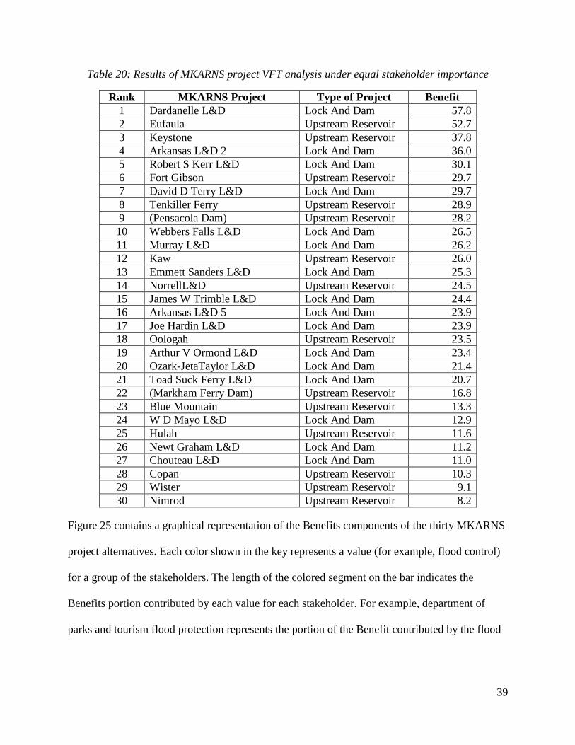
Table 20: Results of MKARNS project VFT analysis under equal stakeholder importance

Rank MKARNS Project Type of Project Benefit

1 Dardanelle L&D Lock And Dam 57.8

2 Eufaula Upstream Reservoir 52.7

3 Keystone Upstream Reservoir 37.8

4 Arkansas L&D 2 Lock And Dam 36.0

5 Robert S Kerr L&D Lock And Dam 30.1

6 Fort Gibson Upstream Reservoir 29.7

7 David D Terry L&D Lock And Dam 29.7

8 Tenkiller Ferry Upstream Reservoir 28.9

9 (Pensacola Dam) Upstream Reservoir 28.2

10 Webbers Falls L&D Lock And Dam 26.5

11 Murray L&D Lock And Dam 26.2

12 Kaw Upstream Reservoir 26.0

13 Emmett Sanders L&D Lock And Dam 25.3

14 NorrellL&D Upstream Reservoir 24.5

15 James W Trimble L&D Lock And Dam 24.4


17 Joe Hardin L&D Lock And Dam 23.9

18 Oologah Upstream Reservoir 23.5

19 Arthur V Ormond L&D Lock And Dam 23.4

20 Ozark-JetaTaylor L&D Lock And Dam 21.4

21 Toad Suck Ferry L&D Lock And Dam 20.7

22 (Markham Ferry Dam) Upstream Reservoir 16.8

23 Blue Mountain Upstream Reservoir 13.3

24 W D Mayo L&D Lock And Dam 12.9

25 Hulah Upstream Reservoir 11.6

26 Newt Graham L&D Lock And Dam 11.2

27 Chouteau L&D Lock And Dam 11.0

28 Copan Upstream Reservoir 10.3

29 Wister Upstream Reservoir 9.1

30 Nimrod Upstream Reservoir 8.2

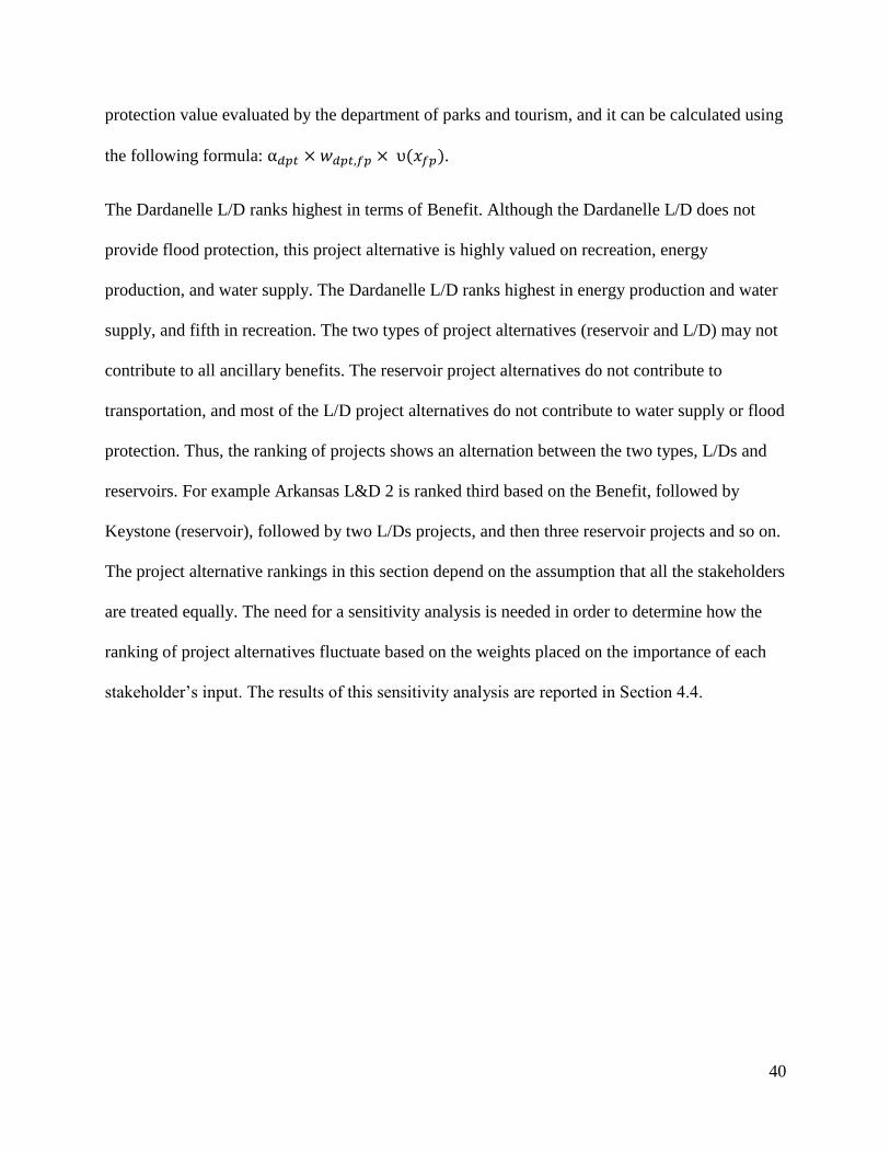
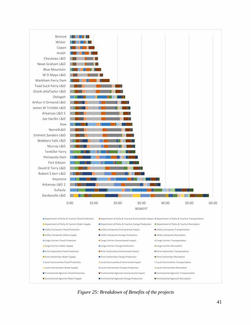
Figure 25 contains a graphical representation of the Benefits components of the thirty MKARNS

project alternatives. Each color shown in the key represents a value (for example, flood control)

for a group of the stakeholders. The length of the colored segment on the bar indicates the

Benefits portion contributed by each value for each stakeholder. For example, department of

parks and tourism flood protection represents the portion of the Benefit contributed by the flood

40

protection value evaluated by the department of parks and tourism, and it can be calculated using

the following formula: α𝑑𝑝𝑡 × 𝑤𝑑𝑝𝑡,𝑓𝑝 × υ(𝑥𝑓𝑝).

The Dardanelle L/D ranks highest in terms of Benefit. Although the Dardanelle L/D does not

provide flood protection, this project alternative is highly valued on recreation, energy

production, and water supply. The Dardanelle L/D ranks highest in energy production and water

supply, and fifth in recreation. The two types of project alternatives (reservoir and L/D) may not

contribute to all ancillary benefits. The reservoir project alternatives do not contribute to

transportation, and most of the L/D project alternatives do not contribute to water supply or flood

protection. Thus, the ranking of projects shows an alternation between the two types, L/Ds and

reservoirs. For example Arkansas L&D 2 is ranked third based on the Benefit, followed by

Keystone (reservoir), followed by two L/Ds projects, and then three reservoir projects and so on.

The project alternative rankings in this section depend on the assumption that all the stakeholders

are treated equally. The need for a sensitivity analysis is needed in order to determine how the

ranking of project alternatives fluctuate based on the weights placed on the importance of each

stakeholder’s input. The results of this sensitivity analysis are reported in Section 4.4.

41

Figure 25: Breakdown of Benefits of the projects

0.00 10.00 20.00 30.00 40.00 50.00 60.00

Dardanelle L&D

Eufaula

Arkansas L&D 2

Keystone

Robert S Kerr L&D

David D Terry L&D

Fort Gibson

Pensacola Dam

Tenkiller Ferry

Murray L&D

Webbers Falls L&D

Emmett Sanders L&D

NorrellL&D

Kaw

Joe Hardin L&D

Arkansas L&D 5

James W Trimble L&D

Arthur V Ormond L&D

Oologah

Ozark-JetaTaylor L&D

Toad Suck Ferry L&D

Markham Ferry Dam

W D Mayo L&D

Blue Mountain

Newt Graham L&D

Chouteau L&D

Hulah

Copan

Wister

Nimrod

BENEFIT

Department of Parks & Tourism Flood Protection Department of Parks & Tourism Enviromental Impact Department of Parks & Tourism Transportation

Department of Parks & Tourism Water Supply Department of Parks & Tourism Energy Production Department of Parks & Tourism Recreation

Utility Companies Flood Protection Utility Companies Enviromental Impact Utility Companies Transportation

Utility Companies Water Supply Utility Companies Energy Production Utility Companies Recreation

Cargo Carriers Flood Protection Cargo Carriers Enviromental Impact Cargo Carriers Transportation

Cargo Carriers Water Supply Cargo Carriers Energy Production Cargo Carriers Recreation

Ports Authorities Flood Protection Ports Authorities Enviromental Impact Ports Authorities Transportation

Ports Authorities Water Supply Ports Authorities Energy Production Ports Authorities Recreation

Local Communities Flood Protection Local Communities Enviromental Impact Local Communities Transportation

Local Communities Water Supply Local Communities Energy Production Local Communities Recreation

Enviromental Agencies Flood Protection Enviromental Agencies Enviromental Impact Enviromental Agencies Transportation

Enviromental Agencies Water Supply Enviromental Agencies Energy Production Enviromental Agencies Recreation

42

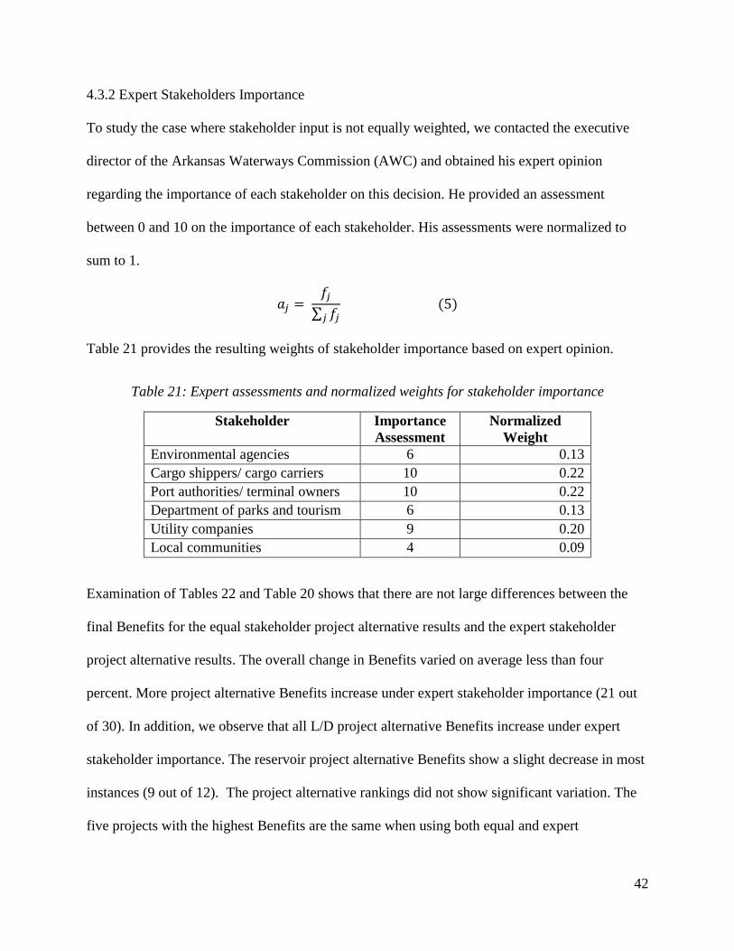
4.3.2 Expert Stakeholders Importance

To study the case where stakeholder input is not equally weighted, we contacted the executive

director of the Arkansas Waterways Commission (AWC) and obtained his expert opinion

regarding the importance of each stakeholder on this decision. He provided an assessment

between 0 and 10 on the importance of each stakeholder. His assessments were normalized to

sum to 1.

𝑎𝑗 = 𝑓𝑗

∑ 𝑓𝑗𝑗 (5)

Table 21 provides the resulting weights of stakeholder importance based on expert opinion.

Table 21: Expert assessments and normalized weights for stakeholder importance

Stakeholder Importance

Assessment

Normalized

Weight

Environmental agencies 6 0.13

Cargo shippers/ cargo carriers 10 0.22

Port authorities/ terminal owners 10 0.22

Department of parks and tourism 6 0.13

Utility companies 9 0.20

Local communities 4 0.09

Examination of Tables 22 and Table 20 shows that there are not large differences between the

final Benefits for the equal stakeholder project alternative results and the expert stakeholder

project alternative results. The overall change in Benefits varied on average less than four

percent. More project alternative Benefits increase under expert stakeholder importance (21 out

of 30). In addition, we observe that all L/D project alternative Benefits increase under expert

stakeholder importance. The reservoir project alternative Benefits show a slight decrease in most

instances (9 out of 12). The project alternative rankings did not show significant variation. The

five projects with the highest Benefits are the same when using both equal and expert

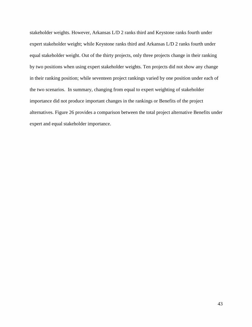
43

stakeholder weights. However, Arkansas L/D 2 ranks third and Keystone ranks fourth under

expert stakeholder weight; while Keystone ranks third and Arkansas L/D 2 ranks fourth under

equal stakeholder weight. Out of the thirty projects, only three projects change in their ranking

by two positions when using expert stakeholder weights. Ten projects did not show any change

in their ranking position; while seventeen project rankings varied by one position under each of

the two scenarios. In summary, changing from equal to expert weighting of stakeholder

importance did not produce important changes in the rankings or Benefits of the project

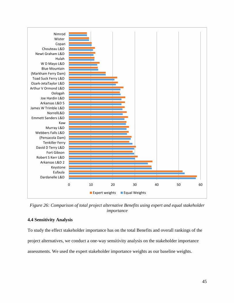
alternatives. Figure 26 provides a comparison between the total project alternative Benefits under

expert and equal stakeholder importance.

44

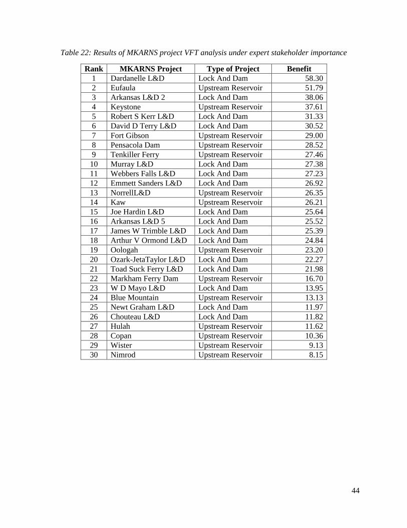
Table 22: Results of MKARNS project VFT analysis under expert stakeholder importance

Rank MKARNS Project Type of Project Benefit

1 Dardanelle L&D Lock And Dam 58.30

2 Eufaula Upstream Reservoir 51.79


4 Keystone Upstream Reservoir 37.61

5 Robert S Kerr L&D Lock And Dam 31.33

6 David D Terry L&D Lock And Dam 30.52

7 Fort Gibson Upstream Reservoir 29.00

8 Pensacola Dam Upstream Reservoir 28.52

9 Tenkiller Ferry Upstream Reservoir 27.46

10 Murray L&D Lock And Dam 27.38

11 Webbers Falls L&D Lock And Dam 27.23

12 Emmett Sanders L&D Lock And Dam 26.92

13 NorrellL&D Upstream Reservoir 26.35

14 Kaw Upstream Reservoir 26.21

15 Joe Hardin L&D Lock And Dam 25.64


17 James W Trimble L&D Lock And Dam 25.39

18 Arthur V Ormond L&D Lock And Dam 24.84

19 Oologah Upstream Reservoir 23.20

20 Ozark-JetaTaylor L&D Lock And Dam 22.27

21 Toad Suck Ferry L&D Lock And Dam 21.98

22 Markham Ferry Dam Upstream Reservoir 16.70

23 W D Mayo L&D Lock And Dam 13.95

24 Blue Mountain Upstream Reservoir 13.13

25 Newt Graham L&D Lock And Dam 11.97

26 Chouteau L&D Lock And Dam 11.82

27 Hulah Upstream Reservoir 11.62

28 Copan Upstream Reservoir 10.36

29 Wister Upstream Reservoir 9.13

30 Nimrod Upstream Reservoir 8.15

45

Figure 26: Comparison of total project alternative Benefits using expert and equal stakeholder

importance

4.4 Sensitivity Analysis

To study the effect stakeholder importance has on the total Benefits and overall rankings of the

project alternatives, we conduct a one-way sensitivity analysis on the stakeholder importance

assessments. We used the expert stakeholder importance weights as our baseline weights.

0 10 20 30 40 50 60

Dardanelle L&D

Eufaula

Keystone

Arkansas L&D 2

Robert S Kerr L&D

Fort Gibson

David D Terry L&D

Tenkiller Ferry

(Pensacola Dam)

Webbers Falls L&D

Murray L&D

Kaw

Emmett Sanders L&D

NorrellL&D

James W Trimble L&D

Arkansas L&D 5

Joe Hardin L&D

Oologah

Arthur V Ormond L&D

Ozark-JetaTaylor L&D

Toad Suck Ferry L&D

(Markham Ferry Dam)

Blue Mountain

W D Mayo L&D

Hulah

Newt Graham L&D

Chouteau L&D

Copan

Wister

Nimrod

Expert weights Equal Weights

46

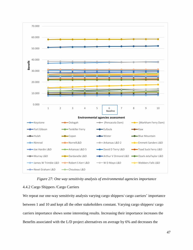
4.4.1 Environmental Agencies

We vary the environmental agencies importance assessment from 1 to 10. As the importance of

environmental agencies increases, the Benefits of the reservoir project alternatives increase,

while eleven out of eighteen L/D project alternative Benefits decrease. There was an average

change on the Benefits of 4.3% when increasing the environmental agencies assessment from 1

to 10. The Markham Ferry project alternative exhibited the greatest increase in Benefit (+19%)

but this did not increase its overall ranking (22th of 30). The Kaw project alternative shows an

increase in its overall ranking from sixteenth to twelfth. Figure 27 shows how Benefits change

for each of the project alternatives based on the change in importance of environmental agencies.

Here we see that the change in the weights of environmental agencies importance does not have

a large influence on the Benefits of the project alternatives.

47

Figure 27: One way sensitivity analysis of environmental agencies importance

4.4.2 Cargo Shippers /Cargo Carriers

We repeat our one-way sensitivity analysis varying cargo shippers/ cargo carriers’ importance

between 1 and 10 and kept all the other stakeholders constant. Varying cargo shippers/ cargo

carriers importance shows some interesting results. Increasing their importance increases the

Benefits associated with the L/D project alternatives on average by 6% and decreases the

0.000

10.000

20.000

30.000

40.000

50.000

60.000

70.000

1 2 3 4 5 6 7 8 9 10

Be

ne

fit

Environmental agancies assessment

Keystone Oologah (Pensacola Dam) (Markham Ferry Dam)

Fort Gibson Tenkiller Ferry Eufaula Kaw

Hulah Copan Wister Blue Mountain

Nimrod NorrellL&D Arkansas L&D 2 Emmett Sanders L&D

Joe Hardin L&D Arkansas L&D 5 David D Terry L&D Toad Suck Ferry L&D

Murray L&D Dardanelle L&D Arthur V Ormond L&D Ozark-JetaTaylor L&D

James W Trimble L&D Robert S Kerr L&D W D Mayo L&D Webbers Falls L&D

Newt Graham L&D Chouteau L&D

Baseline

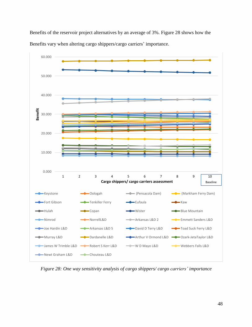
48

Benefits of the reservoir project alternatives by an average of 3%. Figure 28 shows how the

Benefits vary when altering cargo shippers/cargo carriers’ importance.

Figure 28: One way sensitivity analysis of cargo shippers/ cargo carriers’ importance

0.000

10.000

20.000

30.000

40.000

50.000

60.000

1 2 3 4 5 6 7 8 9 10

Be

ne

fit

Cargo shippers/ cargo carriers assessment









Baseline

49

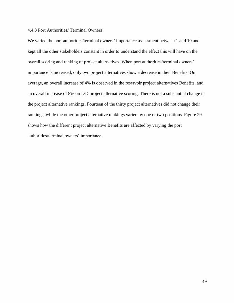
4.4.3 Port Authorities/ Terminal Owners

We varied the port authorities/terminal owners’ importance assessment between 1 and 10 and

kept all the other stakeholders constant in order to understand the effect this will have on the

overall scoring and ranking of project alternatives. When port authorities/terminal owners’

importance is increased, only two project alternatives show a decrease in their Benefits. On

average, an overall increase of 4% is observed in the reservoir project alternatives Benefits, and

an overall increase of 8% on L/D project alternative scoring. There is not a substantial change in

the project alternative rankings. Fourteen of the thirty project alternatives did not change their

rankings; while the other project alternative rankings varied by one or two positions. Figure 29

shows how the different project alternative Benefits are affected by varying the port

authorities/terminal owners’ importance.

50

Figure 29: One way sensitivity analysis of ports authorities/terminal owners’ importance

4.4.4 Department of Parks and Tourism

We vary the department of parks and tourism importance assessment between 1 and 10 in our

next one-way sensitivity analysis. Increasing the importance of department of parks and tourism

decreases the Benefits of the L/D project alternatives by 7% on average. The Benefits of nine of

0.000

10.000

20.000

30.000

40.000

50.000

60.000

1 2 3 4 5 6 7 8 9 10

Be

ne

fit

port authorities/terminal owners assessment

Keystone Oologah (Pensacola Dam)

(Markham Ferry Dam) Fort Gibson Tenkiller Ferry

Eufaula Kaw Hulah

Copan Wister Blue Mountain

Nimrod NorrellL&D Arkansas L&D 2

Emmett Sanders L&D Joe Hardin L&D Arkansas L&D 5

David D Terry L&D Toad Suck Ferry L&D Murray L&D

Dardanelle L&D Arthur V Ormond L&D Ozark-JetaTaylor L&D

James W Trimble L&D Robert S Kerr L&D W D Mayo L&D

Webbers Falls L&D Newt Graham L&D Chouteau L&D

Baseline

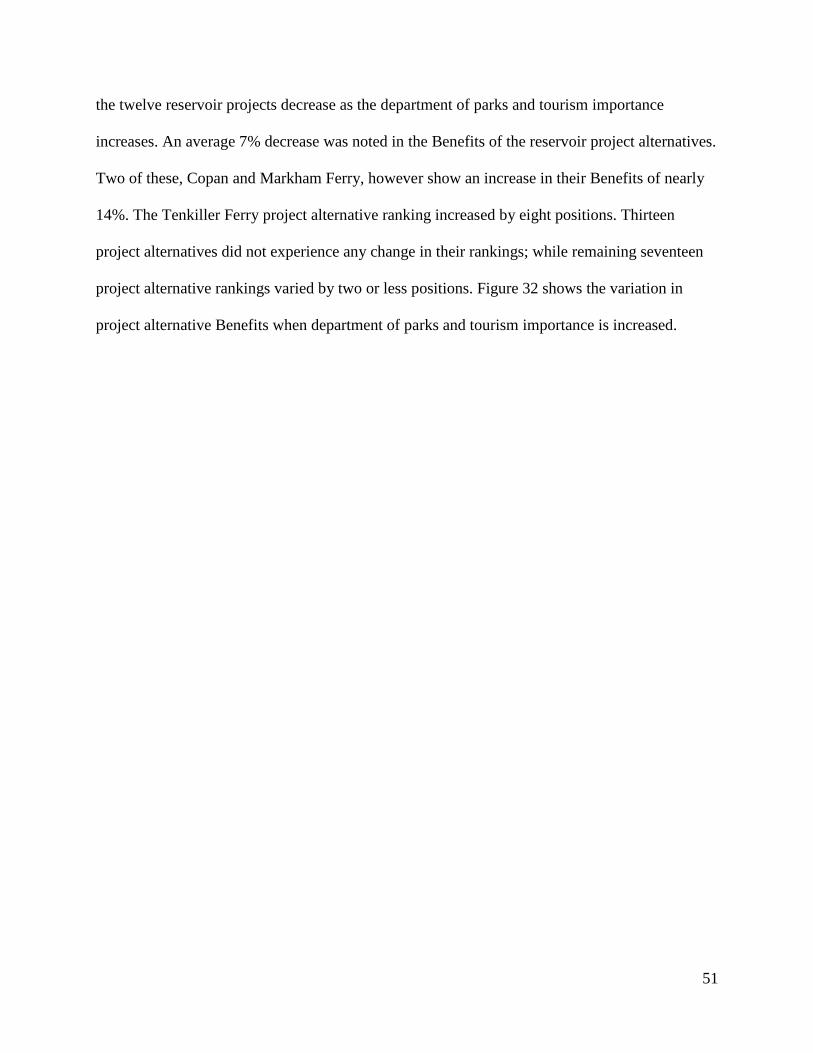
51

the twelve reservoir projects decrease as the department of parks and tourism importance

increases. An average 7% decrease was noted in the Benefits of the reservoir project alternatives.

Two of these, Copan and Markham Ferry, however show an increase in their Benefits of nearly

14%. The Tenkiller Ferry project alternative ranking increased by eight positions. Thirteen

project alternatives did not experience any change in their rankings; while remaining seventeen

project alternative rankings varied by two or less positions. Figure 32 shows the variation in

project alternative Benefits when department of parks and tourism importance is increased.

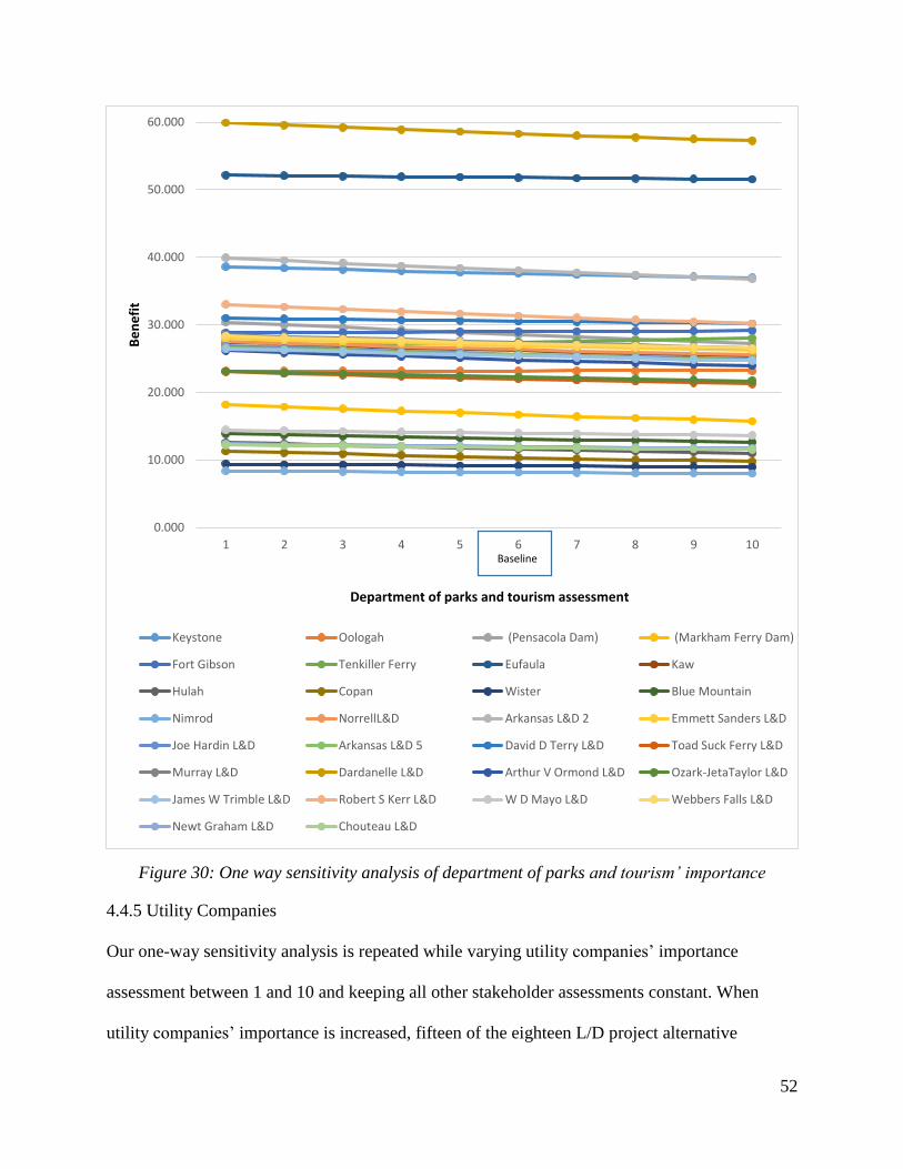
52

Figure 30: One way sensitivity analysis of department of parks and tourism’ importance

4.4.5 Utility Companies

Our one-way sensitivity analysis is repeated while varying utility companies’ importance

assessment between 1 and 10 and keeping all other stakeholder assessments constant. When

utility companies’ importance is increased, fifteen of the eighteen L/D project alternative

0.000

10.000

20.000

30.000

40.000

50.000

60.000

1 2 3 4 5 6 7 8 9 10

Be

ne

fit

Department of parks and tourism assessment









Baseline

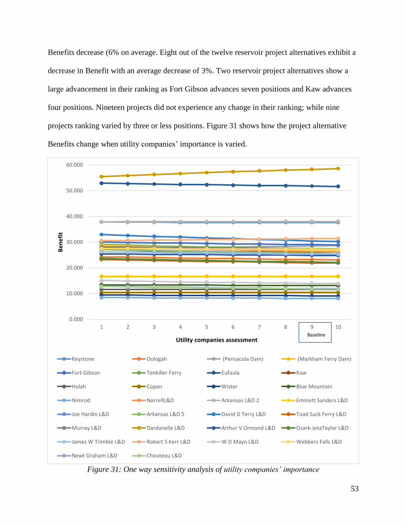
53

Benefits decrease (6% on average. Eight out of the twelve reservoir project alternatives exhibit a

decrease in Benefit with an average decrease of 3%. Two reservoir project alternatives show a

large advancement in their ranking as Fort Gibson advances seven positions and Kaw advances

four positions. Nineteen projects did not experience any change in their ranking; while nine

projects ranking varied by three or less positions. Figure 31 shows how the project alternative

Benefits change when utility companies’ importance is varied.

Figure 31: One way sensitivity analysis of utility companies’ importance

0.000

10.000

20.000

30.000

40.000

50.000

60.000

1 2 3 4 5 6 7 8 9 10

Be

ne

fit

Utility companies assessment









Baseline

54

4.4.6 Local Communities

We repeat our one-way sensitivity analysis by varying the local communities’ importance

assessment between 1 and 10 and keeping all the other stakeholders’ importance assessments

constant in order to understand the effects this will have on the scoring and ranking of project

alternatives. When increasing the local communities’ importance, all L/D project alternative

Benefits decrease except for the Dardanelle L/D. On average, the L/D project alternative

Benefits decrease by 4%. When local communities’ importance is increased, five out of twelve

reservoir project alternative Benefits decreased. The Tenkiller Ferry project alternative exhibits

the largest increase in Benefit (+7%) which causes it to move up five positions in the overall

rankings. All the other project rankings either remained constant or vary no more than two

positions. Figure 30 shows the impact on overall project alternative Benefits when the local

communities’ importance is varied.

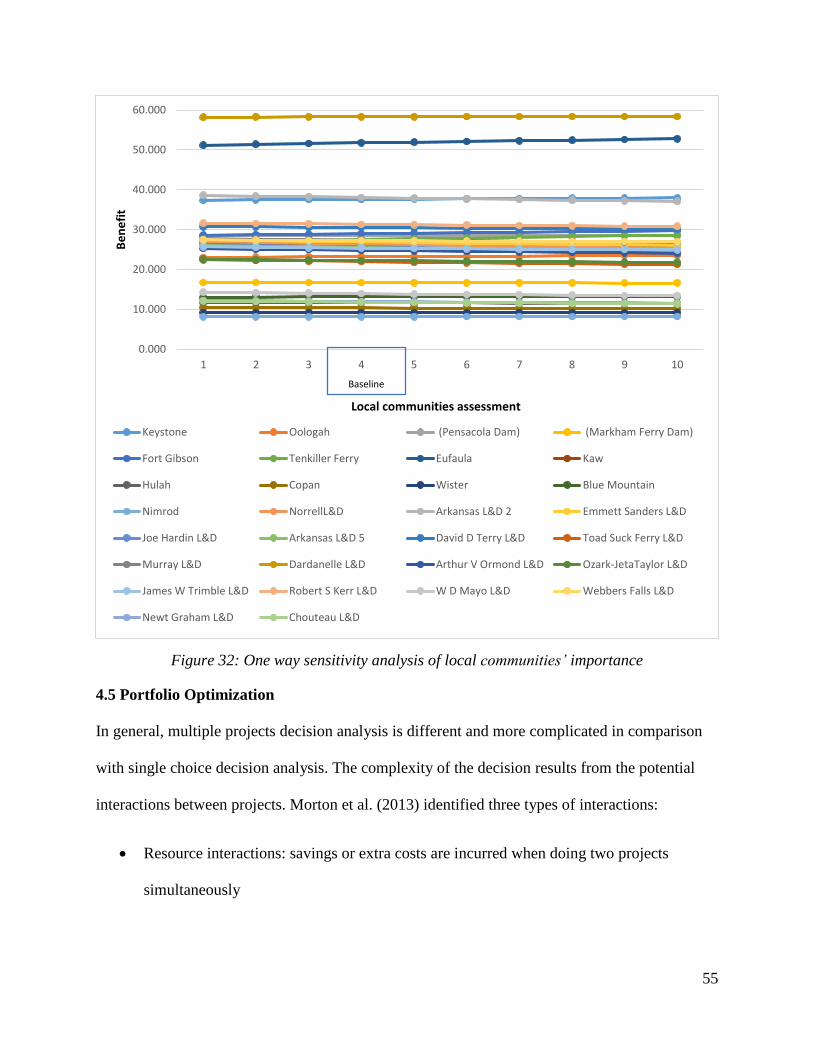
55

Figure 32: One way sensitivity analysis of local communities’ importance

4.5 Portfolio Optimization

In general, multiple projects decision analysis is different and more complicated in comparison

with single choice decision analysis. The complexity of the decision results from the potential

interactions between projects. Morton et al. (2013) identified three types of interactions:

Resource interactions: savings or extra costs are incurred when doing two projects

simultaneously

0.000

10.000

20.000

30.000

40.000

50.000

60.000

1 2 3 4 5 6 7 8 9 10

Be

ne

fit

Local communities assessment









Baseline

Baseline

56

Technical interactions: One project depend on another project or projects are mutually

exclusive

Benefit interactions: Benefits of doing two projects together is different than the sum of

benefits if done individually.

When considering the final allocation of projects, it is important to make sure that the benefits of

multiple projects are balanced and we avoid choosing projects that have the same benefits.

Balance constraints is a common method to balance the project portfolio. This method allows

achievement of a minimum desirable outcome for a particular criterion.

In our inland waterways infrastructure investment model (IWII), we assume that there are no

interactions of any type between our project alternatives. We include balance constraints to attain

a minimum desirable outcome for five of the six values. The objective function of the model is

to maximize the total benefit of a portfolio of IWS infrastructure investment projects. The IWII

model is a binary integer programming model that is formulated as follows:

Sets:

P Set of projects p

I Set of evaluation measures and single dimensional value functions i

J Set of stakeholders j

Parameters:

xip Evaluation measure score of project p for value measure i

Vi(xip): Single dimensional value of value measure i score of project p

wij Weight of the ith single dimensional value for stakeholder j

αj Weight of stakeholder j

B Budget available

Li Minimum acceptable evaluation score for value measure i

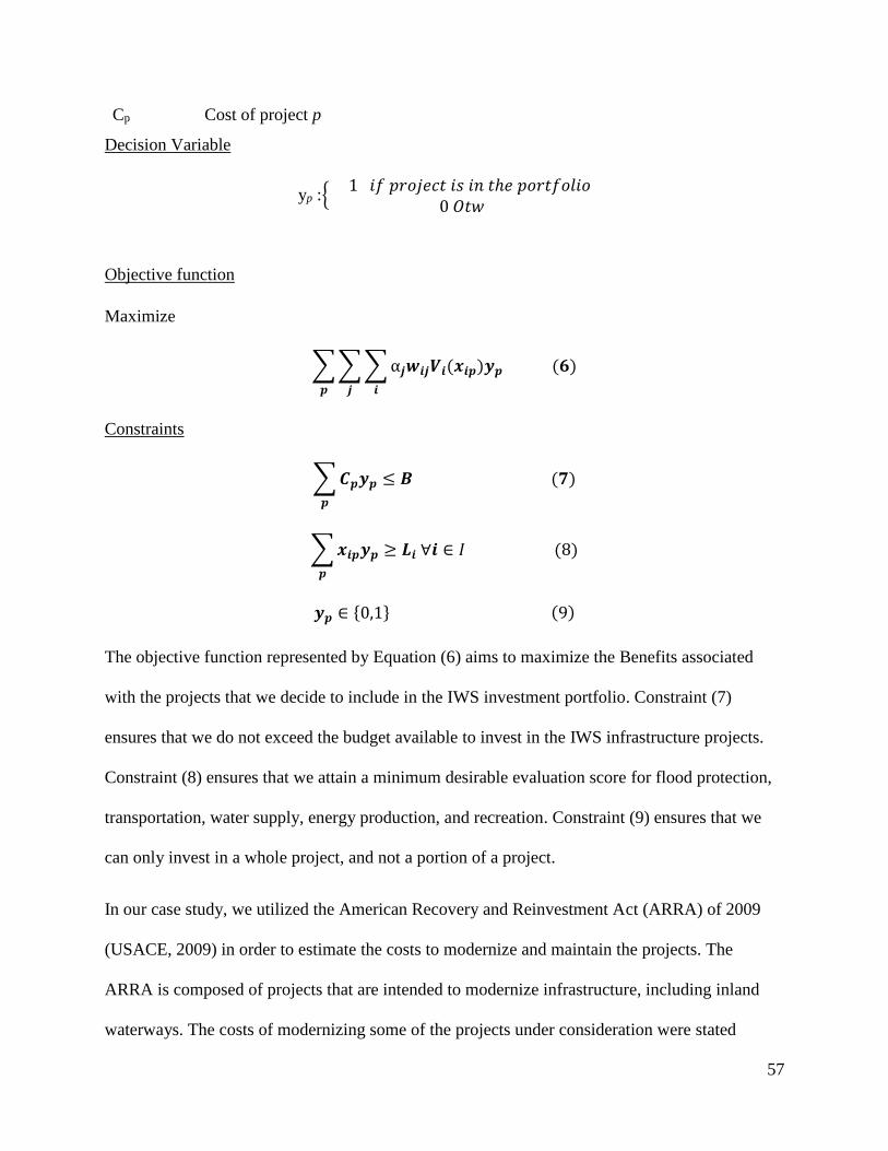
57

Cp Cost of project p

Decision Variable

yp :{ 1 𝑖𝑓 𝑝𝑟𝑜𝑗𝑒𝑐𝑡 𝑖𝑠 𝑖𝑛 𝑡ℎ𝑒 𝑝𝑜𝑟𝑡𝑓𝑜𝑙𝑖𝑜

0 𝑂𝑡𝑤

Objective function

Maximize

∑ ∑ ∑ α𝒋𝒘𝒊𝒋𝑽𝒊(𝒙𝒊𝒑)𝒚𝒑

𝒊𝒋𝒑

(𝟔)

Constraints

∑ 𝑪𝒑𝒚𝒑 ≤ 𝑩 (𝟕)

𝒑

∑ 𝒙𝒊𝒑𝒚𝒑 ≥ 𝑳𝒊 ∀𝒊

𝒑

∈ 𝐼 (8)

𝒚𝒑 ∈ {0,1} (9)

The objective function represented by Equation (6) aims to maximize the Benefits associated

with the projects that we decide to include in the IWS investment portfolio. Constraint (7)

ensures that we do not exceed the budget available to invest in the IWS infrastructure projects.

Constraint (8) ensures that we attain a minimum desirable evaluation score for flood protection,

transportation, water supply, energy production, and recreation. Constraint (9) ensures that we

can only invest in a whole project, and not a portion of a project.

In our case study, we utilized the American Recovery and Reinvestment Act (ARRA) of 2009

(USACE, 2009) in order to estimate the costs to modernize and maintain the projects. The

ARRA is composed of projects that are intended to modernize infrastructure, including inland

waterways. The costs of modernizing some of the projects under consideration were stated

58

separately in the Act. The total cost of modernizing the Arkansas and Oklahoma portions of the

MKARNS was provided. We divided the total cost by the number of L/D projects in the

Arkansas and Oklahoma portion and added it to the projects’ specific costs in order to obtain the

total cost for each project. The Markham Ferry reservoir cost was not given in the Act, so we

used the average cost of modernizing the other reservoirs. Table 23 represents the cost associated

with modernizing each of the projects.

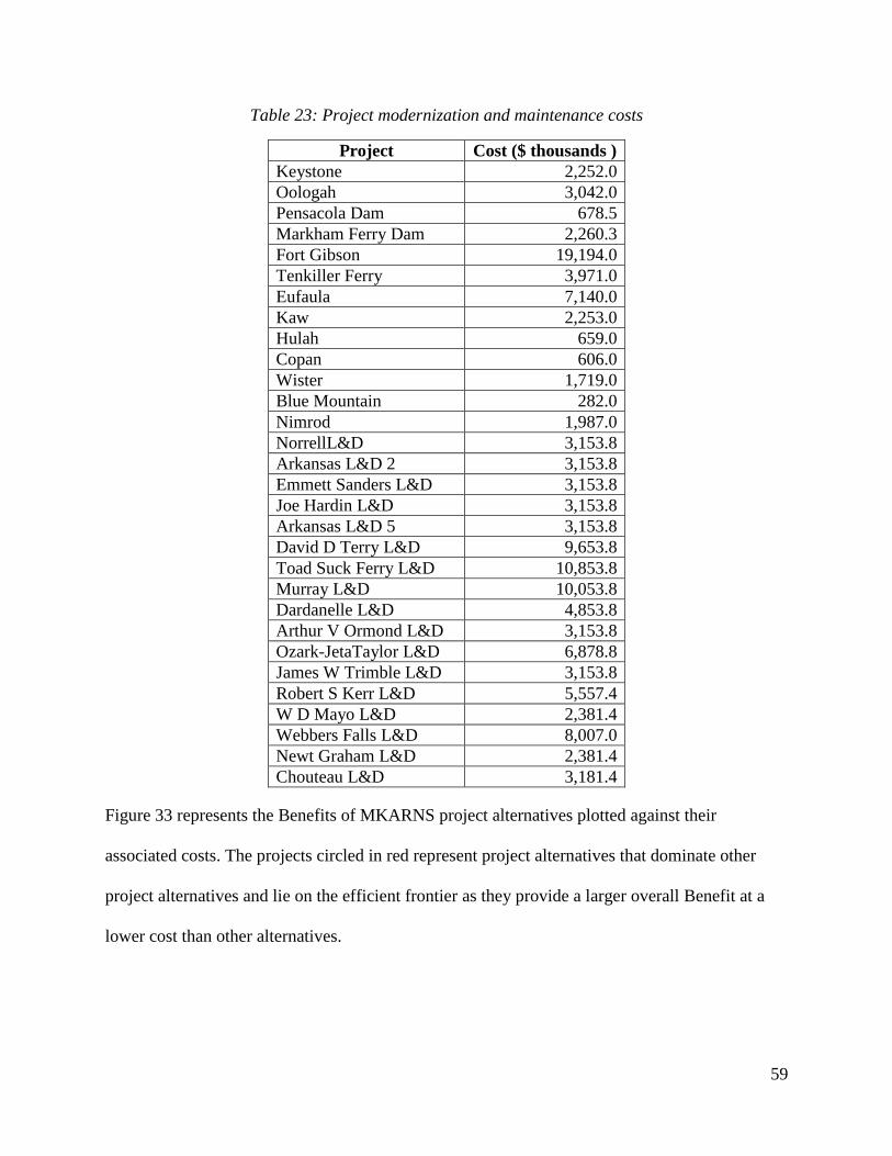
59

Table 23: Project modernization and maintenance costs

Project Cost ($ thousands )

Keystone 2,252.0

Oologah 3,042.0

Pensacola Dam 678.5

Markham Ferry Dam 2,260.3

Fort Gibson 19,194.0

Tenkiller Ferry 3,971.0

Eufaula 7,140.0

Kaw 2,253.0

Hulah 659.0

Copan 606.0

Wister 1,719.0

Blue Mountain 282.0

Nimrod 1,987.0

NorrellL&D 3,153.8

Arkansas L&D 2 3,153.8

Emmett Sanders L&D 3,153.8

Joe Hardin L&D 3,153.8

Arkansas L&D 5 3,153.8

David D Terry L&D 9,653.8

Toad Suck Ferry L&D 10,853.8

Murray L&D 10,053.8

Dardanelle L&D 4,853.8

Arthur V Ormond L&D 3,153.8

Ozark-JetaTaylor L&D 6,878.8

James W Trimble L&D 3,153.8

Robert S Kerr L&D 5,557.4

W D Mayo L&D 2,381.4

Webbers Falls L&D 8,007.0

Newt Graham L&D 2,381.4

Chouteau L&D 3,181.4

Figure 33 represents the Benefits of MKARNS project alternatives plotted against their

associated costs. The projects circled in red represent project alternatives that dominate other

project alternatives and lie on the efficient frontier as they provide a larger overall Benefit at a

lower cost than other alternatives.

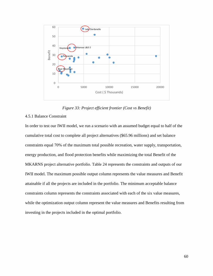
60

Figure 33: Project efficient frontier (Cost vs Benefit)

4.5.1 Balance Constraint

In order to test our IWII model, we run a scenario with an assumed budget equal to half of the

cumulative total cost to complete all project alternatives ($65.96 millions) and set balance

constraints equal 70% of the maximum total possible recreation, water supply, transportation,

energy production, and flood protection benefits while maximizing the total Benefit of the

MKARNS project alternative portfolio. Table 24 represents the constraints and outputs of our

IWII model. The maximum possible output column represents the value measures and Benefit

attainable if all the projects are included in the portfolio. The minimum acceptable balance

constraints column represents the constraints associated with each of the six value measures,

while the optimization output column represent the value measures and Benefits resulting from

investing in the projects included in the optimal portfolio.

0

10

20

30

40

50

60

0 5000 10000 15000 20000

Ben

efit

Cost ( $ Thousands)

Arkansas L&D 2

Pensacola

Blue Mountain

Lake Dardanelle

Keystone

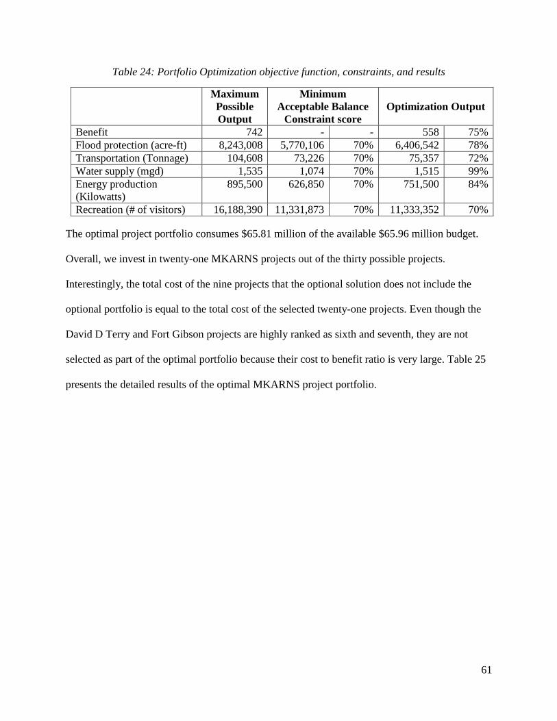
61

Table 24: Portfolio Optimization objective function, constraints, and results

Maximum

Possible

Output

Minimum

Acceptable Balance

Constraint score

Optimization Output

Benefit 742 - - 558 75%

Flood protection (acre-ft) 8,243,008 5,770,106 70% 6,406,542 78%

Transportation (Tonnage) 104,608 73,226 70% 75,357 72%

Water supply (mgd) 1,535 1,074 70% 1,515 99%

Energy production

(Kilowatts)

895,500 626,850 70% 751,500 84%

Recreation (# of visitors) 16,188,390 11,331,873 70% 11,333,352 70%

The optimal project portfolio consumes $65.81 million of the available $65.96 million budget.

Overall, we invest in twenty-one MKARNS projects out of the thirty possible projects.

Interestingly, the total cost of the nine projects that the optional solution does not include the

optional portfolio is equal to the total cost of the selected twenty-one projects. Even though the

David D Terry and Fort Gibson projects are highly ranked as sixth and seventh, they are not

selected as part of the optimal portfolio because their cost to benefit ratio is very large. Table 25

presents the detailed results of the optimal MKARNS project portfolio.

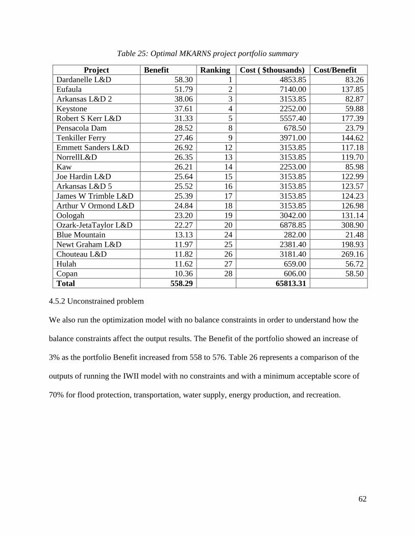
62

Table 25: Optimal MKARNS project portfolio summary

Project Benefit Ranking Cost ( $thousands) Cost/Benefit

Dardanelle L&D 58.30 1 4853.85 83.26

Eufaula 51.79 2 7140.00 137.85

Arkansas L&D 2 38.06 3 3153.85 82.87

Keystone 37.61 4 2252.00 59.88

Robert S Kerr L&D 31.33 5 5557.40 177.39

Pensacola Dam 28.52 8 678.50 23.79

Tenkiller Ferry 27.46 9 3971.00 144.62

Emmett Sanders L&D 26.92 12 3153.85 117.18

NorrellL&D 26.35 13 3153.85 119.70

Kaw 26.21 14 2253.00 85.98

Joe Hardin L&D 25.64 15 3153.85 122.99

Arkansas L&D 5 25.52 16 3153.85 123.57

James W Trimble L&D 25.39 17 3153.85 124.23

Arthur V Ormond L&D 24.84 18 3153.85 126.98

Oologah 23.20 19 3042.00 131.14

Ozark-JetaTaylor L&D 22.27 20 6878.85 308.90

Blue Mountain 13.13 24 282.00 21.48

Newt Graham L&D 11.97 25 2381.40 198.93

Chouteau L&D 11.82 26 3181.40 269.16

Hulah 11.62 27 659.00 56.72

Copan 10.36 28 606.00 58.50

Total 558.29 65813.31

4.5.2 Unconstrained problem

We also run the optimization model with no balance constraints in order to understand how the

balance constraints affect the output results. The Benefit of the portfolio showed an increase of

3% as the portfolio Benefit increased from 558 to 576. Table 26 represents a comparison of the

outputs of running the IWII model with no constraints and with a minimum acceptable score of

70% for flood protection, transportation, water supply, energy production, and recreation.

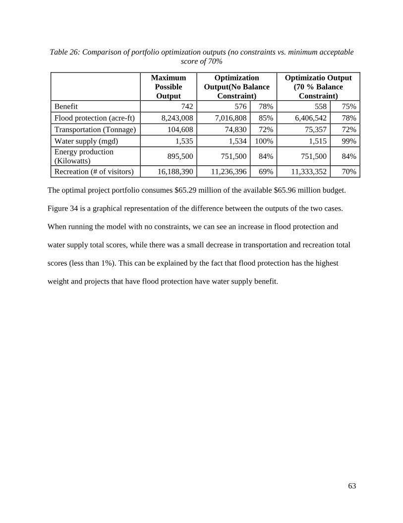
63

Table 26: Comparison of portfolio optimization outputs (no constraints vs. minimum acceptable

score of 70%

Maximum

Possible

Output

Optimization

Output(No Balance

Constraint)

Optimizatio Output

(70 % Balance

Constraint)

Benefit 742 576 78% 558 75%

Flood protection (acre-ft) 8,243,008 7,016,808 85% 6,406,542 78%

Transportation (Tonnage) 104,608 74,830 72% 75,357 72%

Water supply (mgd) 1,535 1,534 100% 1,515 99%

Energy production

(Kilowatts) 895,500 751,500 84% 751,500 84%

Recreation (# of visitors) 16,188,390 11,236,396 69% 11,333,352 70%

The optimal project portfolio consumes $65.29 million of the available $65.96 million budget.

Figure 34 is a graphical representation of the difference between the outputs of the two cases.

When running the model with no constraints, we can see an increase in flood protection and

water supply total scores, while there was a small decrease in transportation and recreation total

scores (less than 1%). This can be explained by the fact that flood protection has the highest

weight and projects that have flood protection have water supply benefit.

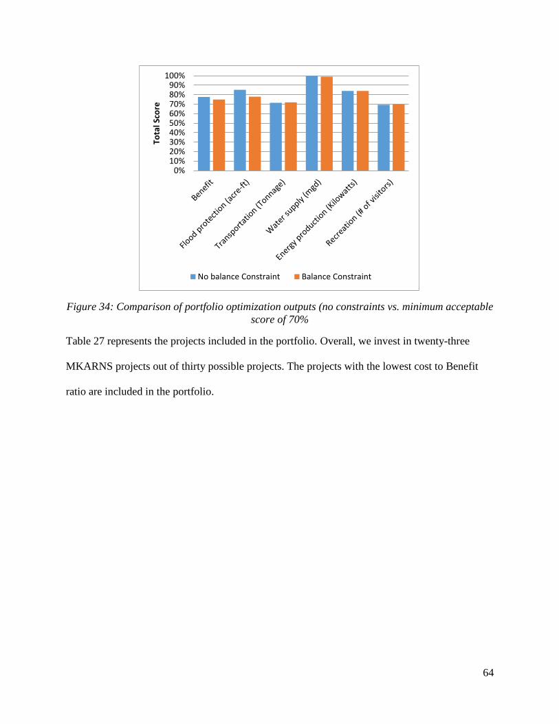
64

Figure 34: Comparison of portfolio optimization outputs (no constraints vs. minimum acceptable

score of 70%

Table 27 represents the projects included in the portfolio. Overall, we invest in twenty-three

MKARNS projects out of thirty possible projects. The projects with the lowest cost to Benefit

ratio are included in the portfolio.

0%10%20%30%40%50%60%70%80%90%

100%

Tota

l Sco

re

No balance Constraint Balance Constraint

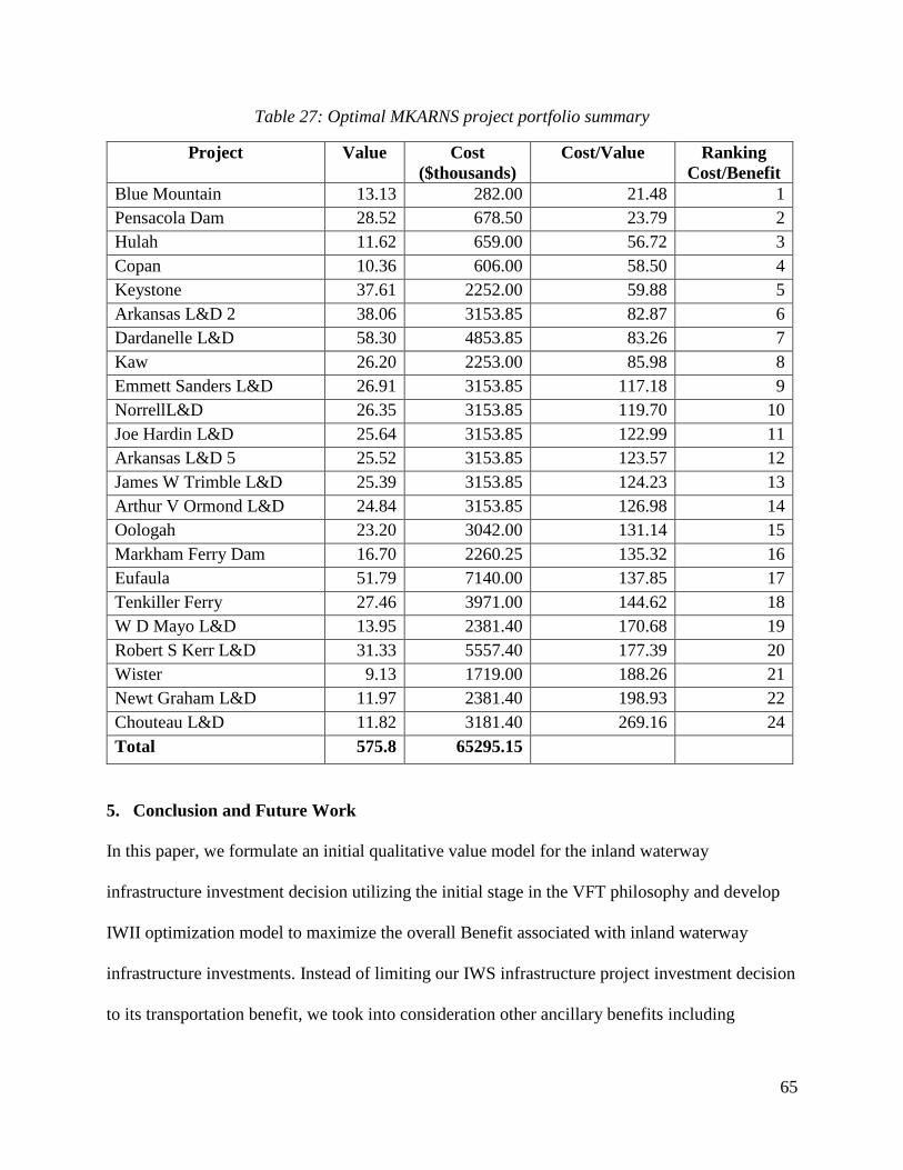
65

Table 27: Optimal MKARNS project portfolio summary

Project Value Cost

($thousands)

Cost/Value Ranking

Cost/Benefit

Blue Mountain 13.13 282.00 21.48 1

Pensacola Dam 28.52 678.50 23.79 2

Hulah 11.62 659.00 56.72 3

Copan 10.36 606.00 58.50 4

Keystone 37.61 2252.00 59.88 5

Arkansas L&D 2 38.06 3153.85 82.87 6

Dardanelle L&D 58.30 4853.85 83.26 7

Kaw 26.20 2253.00 85.98 8

Emmett Sanders L&D 26.91 3153.85 117.18 9

NorrellL&D 26.35 3153.85 119.70 10

Joe Hardin L&D 25.64 3153.85 122.99 11

Arkansas L&D 5 25.52 3153.85 123.57 12

James W Trimble L&D 25.39 3153.85 124.23 13

Arthur V Ormond L&D 24.84 3153.85 126.98 14

Oologah 23.20 3042.00 131.14 15

Markham Ferry Dam 16.70 2260.25 135.32 16

Eufaula 51.79 7140.00 137.85 17

Tenkiller Ferry 27.46 3971.00 144.62 18

W D Mayo L&D 13.95 2381.40 170.68 19

Robert S Kerr L&D 31.33 5557.40 177.39 20

Wister 9.13 1719.00 188.26 21

Newt Graham L&D 11.97 2381.40 198.93 22

Chouteau L&D 11.82 3181.40 269.16 24

Total 575.8 65295.15

5. Conclusion and Future Work

In this paper, we formulate an initial qualitative value model for the inland waterway

infrastructure investment decision utilizing the initial stage in the VFT philosophy and develop

IWII optimization model to maximize the overall Benefit associated with inland waterway

infrastructure investments. Instead of limiting our IWS infrastructure project investment decision

to its transportation benefit, we took into consideration other ancillary benefits including

66

recreation, water supply, energy production, impact on fish and wildlife, and flood protection.

From the literature search, we found that there is no prior published research that incorporates

these multiple IWS ancillary benefits into a single decision model to evaluate IWS infrastructure

investments. This paper proposes a new methodology to evaluate the Benefit of IWS

infrastructure using a VFT philosophy and multiple objective decision optimization.

In this research effort, we attempt to capture the stakeholder opinion on how they value each of

the six ancillary benefits that were assessed. One challenge in conducting this research was

accurately capturing the expert opinion of these values. The importance of ancillary benefits

differs among IWS stakeholders. One common assessment among all IWS stakeholders is highly

valuing flood protection. Another challenge was the assessment of the level of importance placed

on each stakeholder. First, we examined the case when all the stakeholders were considered

equally important in the decision, and then we examined a second scenario where expert opinion

of stakeholder importance was applied. These two assumptions did not show important

differences in the final MKARNS project alternative scoring or rankings, which led us conduct a

set of one-way sensitivity analyses to understand the effects of stakeholders’ importance on the

Benefits and ranking of the project alternatives. As a whole, the one-way sensitivity analysis

shows that the stakeholder importance does not have a significant effect on the scoring or

ranking results. Once the MKARNS project alternatives were evaluated using our VFT

approach, a binary integer programming portfolio optimization model was employed to

maximize the total Benefit of the portfolio while taking in consideration budget and balance

constraints.

There are multiple opportunities to further develop the model present in this paper. The first

potential area for future work is to further examine if linear functions represent the true shape of

67

the value functions: linear, convex, concave or an S-curve for all the value measures. Another

area of potential model improvement is to consider the interactions between the different

projects. The current IWII model assumes that there are no resources, technical, or benefits

interactions between the project alternatives. It is anticipated that difficulties will arise in located

the historical data necessary to make these improvement but further expert input could

potentially enhance the model’s representation of the IWS.

To conclude, the developed value-focused, multi objective portfolio optimization model is a

useful approach in selecting a portfolio of IWS project investments. This methodology allows us

to maximize the total Benefit associated with the project investments while taking in

consideration the necessary budgetary constraints and minimally acceptable IWS benefit

evaluation scores constraints. The developed model allows us to identify a combination of

projects that maximize the total system benefits instead of considering each project individually.

68

References

American Waterways Operators (2013). Jobs and economy: Industry facts. Retrieved January 10,

2015 from http://www.americanwaterways.com/initiatives/jobs-economy/industry-facts .

Axtell, P. G. (2011). Value focused thinking analysis of the Pacific Theater’s future air mobility

en route system. (Master thesis). Air Force Institute of Technology, Wright-Patterson

Air Force Base, Ohio.

Bray, L. G., Murphree, M., & Dager, C. A. (2011). Toward a full accounting of the beneficiaries

of navigable waterways. Center for Transportation Research. The University of

Tennessee.

Chambers, M., & Liu, M. (2012). Maritime trade and transportation by the numbers. Bureau of

Transportation Statistics. Retrieved January 27, 2015, from

http://www.rita.dot.gov/bts/sites/rita.dot.gov.bts/files/publications/by_the_numbers/mari

time_trade_and_transportation/index.html.

Guler, C. U., Johnson, A. W., & Cooper, M. (2012). Case study: Energy industry economic

impacts from Ohio River transportation disruption. The Engineering Economist 57:2, 77-

100.

Iowa Department of Transportation (2008). Barge comparison. Retrieved from

http://www.iowadot.gov/compare.pdf.

Jacobs Engineering U.K. (2011). The value of inland waterways in England and Wales.

Department of Food, Environment and Rural affairs.

Jordan, J. D. (2012). A value focused thinking tutorial for supply chain application. In the

average network flow problem: Shortest path and minimum cost flow formulations,

algorithms, heuristics, and complexity. (Doctoral dissertation). Air Force Institute of

Technology, Wright-Patterson Air Force Base, Ohio.

Katzer, D. J. (2002). Decision analysis with value-focused thinking as a methodology in

structuring the civil engineering operations flight. (Master thesis). Air Force Institute of

Technology, Wright-Patterson Air Force Base, Ohio.

Keeney, R.L. (1992). Value-focused thinking: a path to creative decision making. Cambridge,

Massachusetts: Harvard University Press.

King, C. (2012) Waterway fact sheet. McClellan-Kerr Arkansas River Navigation System.

Oklahoma Department of Transportation. Retrieved January 15, 2015, from

http://www.okladot.state.ok.us/newsmedia/i40bridge/pdfs/Waterways_Barge_Informatio

n.pdf.

Kirkwood, C.W. (1997). Strategic decision making, multi objective decision analysis with

spreadsheets. Belmont: Wadsworth Publishing Company.

http://www.americanwaterways.com/initiatives/jobs-economy/industry-facts

69

Morton, A., Keisler, J., & Salo, A. (2013). Multicriteria portfolio decision analysis for project

selection. The management science group, department of management. London school

of economics and political science.

Nachtmann, H., & Celikkol, S. (2007). Ancillary benefits of the Ouachita River navigation

system.

Nachtmann, H., & Pohl, E.A. (2013). Transportation readiness assessment and valuation for

emergency logistics. International Journal of Emergency Management, Vol. 9, No. 1

(2013).

Neiger, D., Rotaru, K., & Churilov, L. (2009). Supply chain risk identification with value-

focused process engineering. Journal of Operations Management, 27, 154-168.

Oklahoma Department of Transportation (2014). 2014 inland waterway factsheet. Retrieved

January 15, 2015, from

http://www.okladot.state.ok.us/waterway/pdfs/fact_sheet_2014.pdf.

Olson, D. L., & Wu, D. (2010). Enterprise risk management models. Berlin Heidelberg:

Springer-Verlag.

Parnell, G. S. (2007). Chapter 19, Value-focused thinking, methods for conducting military

operational analysis. Military Operations Research Society. Editors Andrew Loerch and

Larry Rainey 2007, pp. 619-656.

Parnell, G. S., Hughes, D. W., Burk, R. C., Driscoll, P. J., Kucik, P. D., Morales, B. L., & Nunn,

L. R. (2013). Survey of value-focused thinking: Applications, research development and

areas for future research. Journal of Multi-criteria Decision Analysis, 20, 49-60.

United Nations Conference on Trade and Development (2014). Review of maritime transport

2013. United Nations publication. Sales No. E.13.II.D.9. New York and Geneva.

United States Army Corps of Engineers (USACE) (2005). Arkansas River navigation study

FEIS: Chapter 4.

USACE (2009). American recovery and reinvestment act of 2009- Civil works expenditure plan

operations and maintenance.

United States Army Corps of Engineers (2010). Recreation program statistics. Retrieved January

15, 2015 from

http://corpslakes.usace.army.mil/visitors/pdfs/RecreationProgramStatistics.pdf.

USACE (2012-1). Little Rock district water management. Retrieved February 11, 2015 from:

http://www.swl-wc.usace.army.mil/pages/AboutRCB.htm.

USACE (2012-2).Recreation fast fact. Retrieved February 15, 2015 from

http://www.corpsresults.us/recreation/recfastfacts.cfm.

http://corpslakes.usace.army.mil/visitors/pdfs/RecreationProgramStatistics.pdf

70

USACE (2013-1). Value to the nation of the USACE’ civil works programs. Retrieved January

30, 2015 from www.iwr.usace.army.mil/ .

USACE (2013-2). USACE hydropower- renewable, reliable, energy independence for America.

Retrieved January 28, 2015 from

www.iwr.usace.army.mil/http://www.usace.army.mil/Portals/2/docs/civilworks/budget/s

trongpt/fy2014sp_hydropower.pdf.

USACE (2013-3).McClellan-Kerr Arkansas River Navigation System. A model system -

resilient, reliable and sustainable. Tulsa district project update. Retrieved February 10,

2015 from http://www.swt.usace.army.mil/Portals/41/docs/library/proj-upd/2013-02.pdf.

USACE (2013-4).Water supply fast fact. Retrieved May 15, 2015 from

http://www.corpsresults.us/watersupply/state.cfml

USACE. Water levels. Retrieved May 15, 2015 from

http://www.swl.usace.army.mil/Missions/WaterLevels.aspx

U.S. Department of Transportation (2013). Tonnage on highways, railroads, and inland

waterways: 2010 Map. Available from:

http://www.ops.fhwa.dot.gov/Freight/freight_analysis/nat_freight_stats/tonhwyrrww201

0.htm.

U.S. Energy Information Administration (2011). Direct federal financial interventions and

subsidies in energy in fiscal year 2010.

U.S. Government Accountability Office (2011). Surface freight transportation: A comparison of

the costs of road, rail, and waterways freight shipments that are not passed on to

consumers.

Reynolds, J. (2013). Hydroelectricity. The Encyclopedia of Arkansas History and Culture.

Retrieved February 13, 2015 from:

http://www.encyclopediaofarkansas.net/encyclopedia/entry-detail.aspx?entryID=5527.

Salo, A., Keisler, J., & Morton, A. (2011). Portfolio decision analysis: Improved methods for

resource allocation, Springer, New York.

Sudar, A., (2005). Measuring non-traditional benefits and cost of inland navigation. Transport.

Res. Board, 3: 47-53.

Texas Transportation Institute (2012). Waterways working for America. Center for Ports and

Waterways. Retrieved February 26, 2015 from

http://www.nationalwaterwaysfoundation.org/study/NWF_117900_2011WorkingForAm

ericaBrochure_FINAL_forWeb.pdf.

Tong, J., Nachtmann, H., & Pohl, E.A. (2013). Value-focused thinking for inland waterborne

cargo prioritization, American Society for Engineering Management Conference

Proceedings, October 2013.

http://www.iwr.usace.army.mil/

http://www.iwr.usace.army.mil/

http://www.swt.usace.army.mil/Portals/41/docs/library/proj-upd/2013-02.pdf

http://www.corpsresults.us/watersupply/state.cfml

http://www.ops.fhwa.dot.gov/Freight/freight_analysis/nat_freight_stats/tonhwyrrww2010.htm

http://www.ops.fhwa.dot.gov/Freight/freight_analysis/nat_freight_stats/tonhwyrrww2010.htm

http://www.eia.gov/analysis/requests/subsidy/

http://www.eia.gov/analysis/requests/subsidy/

71

Town and Country Planning Association (2009). Policy advice note: inland waterways unlocking

the potential and securing the future of inland waterways through the planning system.

Retrieved March 10, 2015 from: https://canalrivertrust.org.uk/media/library/544.pdf.

Waterways Council, Inc. (2013). State profile Arkansas. Retrieved February 26, 2015 from

http://waterwayscouncil.org/wp-content/uploads/2013/03/arkansas-2011.pdf.

Walker, W. (2007). Inland waterway transportation economics program. USACE inland

community of practice workshop. Retrieved January 14, 2015 from

http://www.lrd.usace.army.mil/Portals/73/docs/Navigation/PCXIN/Inland-Wwy-Trans-

Prog_2007-09-20.pdf.

Winthrop, M. F. (1999). Technology selection for the air force research laboratory air vehicles

directorate: An analysis using value focused thinking. (Master thesis). Air Force

Institute of Technology, Wright-Patterson Air Force Base, Ohio.

World Wide Inland Navigation Network. (n.d.). U.S. inland waterways. Retrieved January 15,

2015, from http://www.wwinn.org/us-inland-waterways.

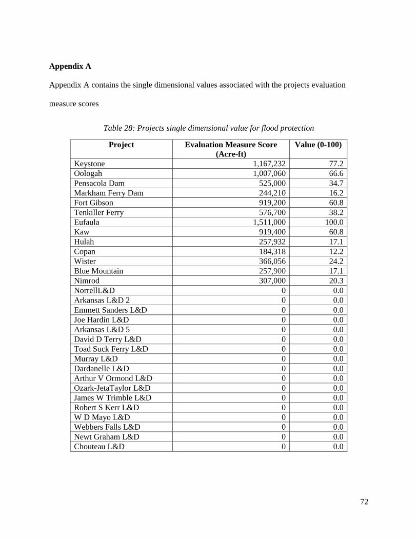
http://www.lrd.usace.army.mil/Portals/73/docs/Navigation/PCXIN/Inland-Wwy-Trans-Prog_2007-09-20.pdf

http://www.lrd.usace.army.mil/Portals/73/docs/Navigation/PCXIN/Inland-Wwy-Trans-Prog_2007-09-20.pdf

72

Appendix A

Appendix A contains the single dimensional values associated with the projects evaluation

measure scores

Table 28: Projects single dimensional value for flood protection

Project Evaluation Measure Score

(Acre-ft)

Value (0-100)

Keystone 1,167,232 77.2

Oologah 1,007,060 66.6

Pensacola Dam 525,000 34.7

Markham Ferry Dam 244,210 16.2

Fort Gibson 919,200 60.8

Tenkiller Ferry 576,700 38.2

Eufaula 1,511,000 100.0

Kaw 919,400 60.8

Hulah 257,932 17.1

Copan 184,318 12.2

Wister 366,056 24.2

Blue Mountain 257,900 17.1

Nimrod 307,000 20.3

NorrellL&D 0 0.0

Arkansas L&D 2 0 0.0

Emmett Sanders L&D 0 0.0

Joe Hardin L&D 0 0.0


David D Terry L&D 0 0.0

Toad Suck Ferry L&D 0 0.0

Murray L&D 0 0.0

Dardanelle L&D 0 0.0

Arthur V Ormond L&D 0 0.0

Ozark-JetaTaylor L&D 0 0.0

James W Trimble L&D 0 0.0

Robert S Kerr L&D 0 0.0

W D Mayo L&D 0 0.0

Webbers Falls L&D 0 0.0

Newt Graham L&D 0 0.0

Chouteau L&D 0 0.0

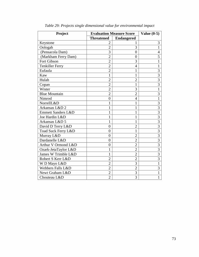
73

Table 29: Projects single dimensional value for environmental impact

Project Evaluation Measure Score Value (0-5)

Threatened Endangered

Keystone 2 1 3

Oologah 2 3 1

(Pensacola Dam) 3 0 4

(Markham Ferry Dam) 2 0 5

Fort Gibson 2 3 1

Tenkiller Ferry 2 4 1

Eufaula 2 1 3

Kaw 1 1 3

Hulah 2 2 3

Copan 2 1 3

Wister 2 3 1

Blue Mountain 2 2 3

Nimrod 0 4 1

NorrellL&D 1 1 3

Arkansas L&D 2 1 1 3

Emmett Sanders L&D 1 1 3

Joe Hardin L&D 1 1 3

Arkansas L&D 5 1 1 3

David D Terry L&D 0 2 3

Toad Suck Ferry L&D 0 1 3

Murray L&D 0 2 3

Dardanelle L&D 0 2 3

Arthur V Ormond L&D 0 2 3

Ozark-JetaTaylor L&D 1 2 3

James W Trimble L&D 1 2 3

Robert S Kerr L&D 2 2 3

W D Mayo L&D 2 3 1

Webbers Falls L&D 2 2 3

Newt Graham L&D 2 3 1

Chouteau L&D 2 3 1

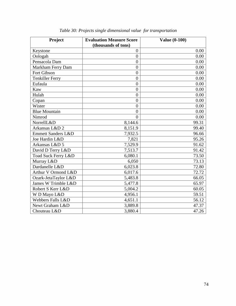
74

Table 30: Projects single dimensional value for transportation


(thousands of tons)

Value (0-100)

Keystone 0 0.00

Oologah 0 0.00

Pensacola Dam 0 0.00

Markham Ferry Dam 0 0.00

Fort Gibson 0 0.00

Tenkiller Ferry 0 0.00

Eufaula 0 0.00

Kaw 0 0.00

Hulah 0 0.00

Copan 0 0.00

Wister 0 0.00

Blue Mountain 0 0.00

Nimrod 0 0.00

NorrellL&D 8,144.6 99.31

Arkansas L&D 2 8,151.9 99.40

Emmett Sanders L&D 7,932.5 96.66

Joe Hardin L&D 7,821 95.26

Arkansas L&D 5 7,529.9 91.62

David D Terry L&D 7,513.7 91.42

Toad Suck Ferry L&D 6,080.1 73.50

Murray L&D 6,050 73.13

Dardanelle L&D 6,023.8 72.80

Arthur V Ormond L&D 6,017.6 72.72

Ozark-JetaTaylor L&D 5,483.8 66.05

James W Trimble L&D 5,477.8 65.97

Robert S Kerr L&D 5,004.2 60.05

W D Mayo L&D 4,956.1 59.51

Webbers Falls L&D 4,651.1 56.12

Newt Graham L&D 3,889.8 47.37

Chouteau L&D 3,880.4 47.26

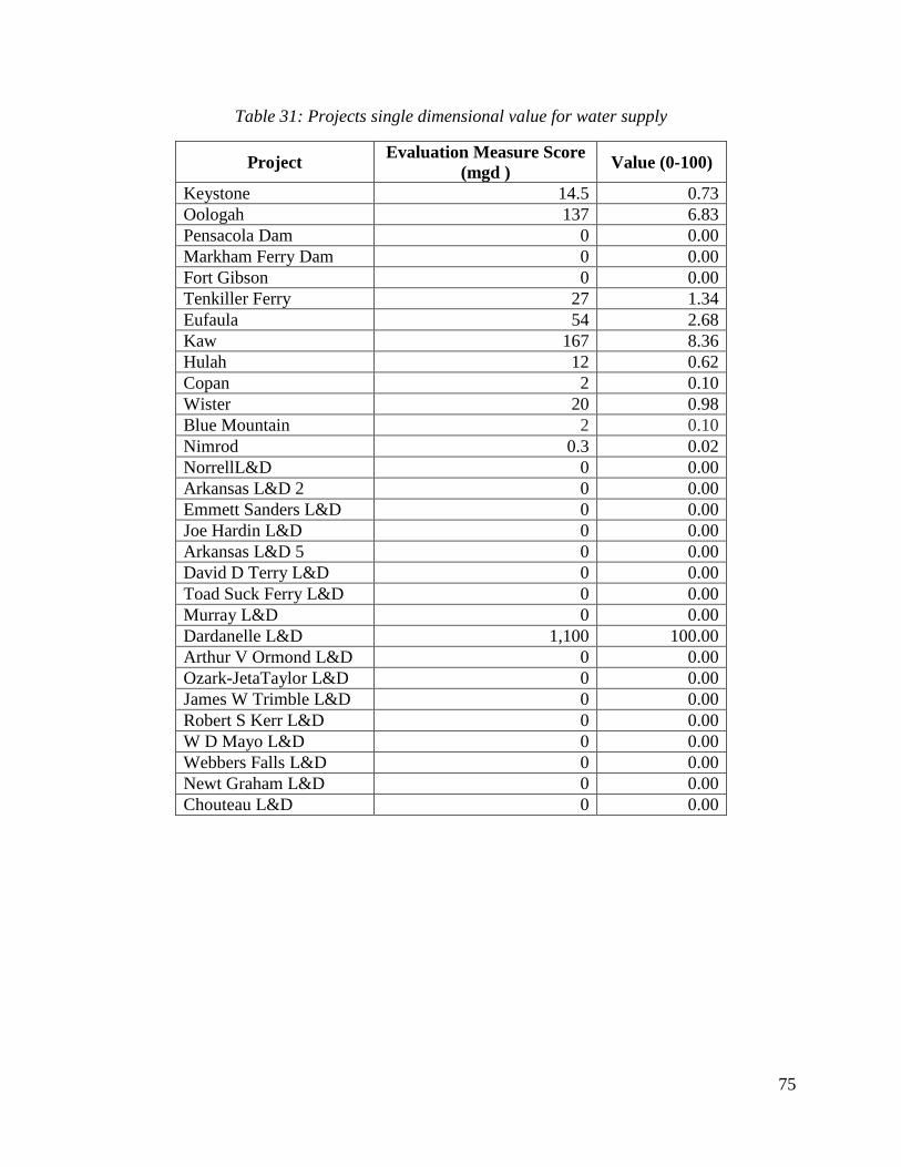
75

Table 31: Projects single dimensional value for water supply


(mgd ) Value (0-100)

Keystone 14.5 0.73

Oologah 137 6.83

Pensacola Dam 0 0.00


Fort Gibson 0 0.00

Tenkiller Ferry 27 1.34

Eufaula 54 2.68

Kaw 167 8.36

Hulah 12 0.62

Copan 2 0.10

Wister 20 0.98


Nimrod 0.3 0.02

NorrellL&D 0 0.00







Murray L&D 0 0.00

Dardanelle L&D 1,100 100.00

Arthur V Ormond L&D 0 0.00


James W Trimble L&D 0 0.00

Robert S Kerr L&D 0 0.00

W D Mayo L&D 0 0.00

Webbers Falls L&D 0 0.00


Chouteau L&D 0 0.00

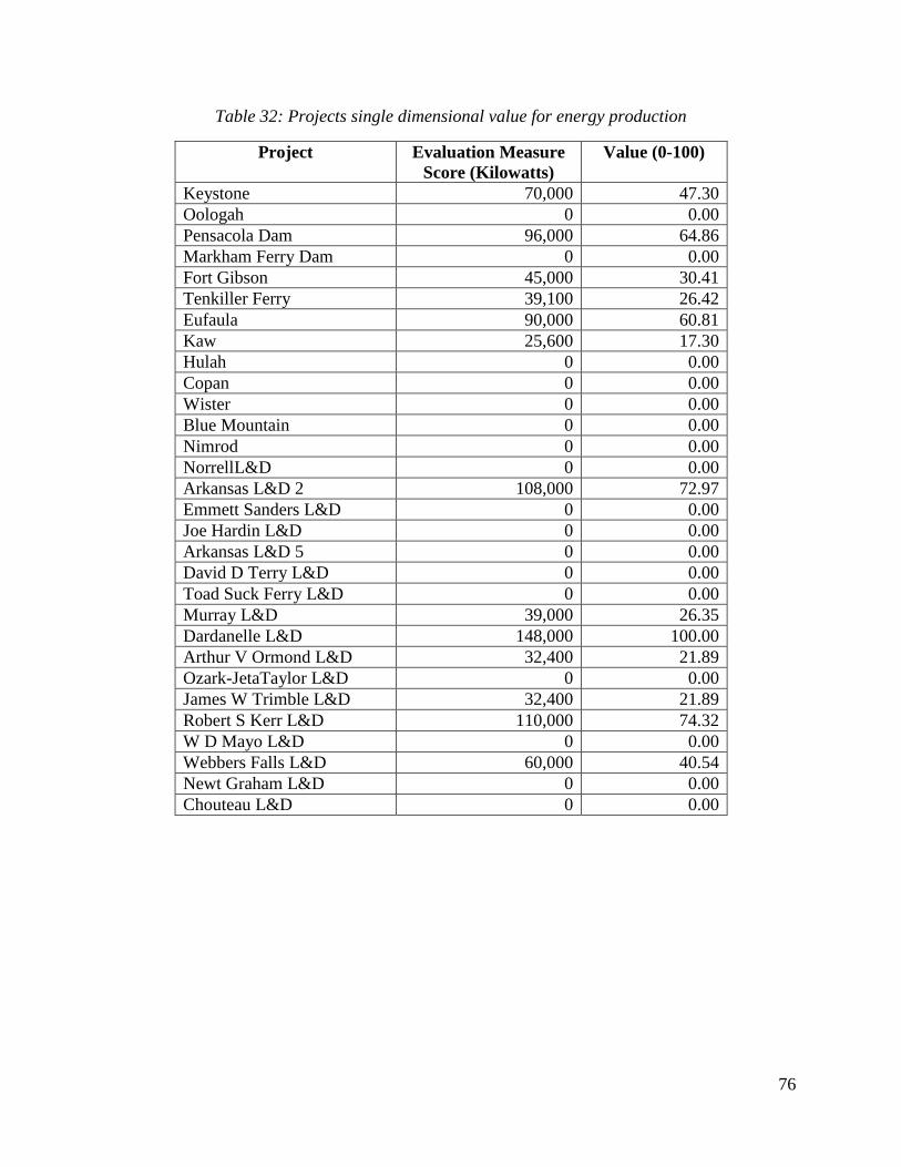
76

Table 32: Projects single dimensional value for energy production

Project Evaluation Measure

Score (Kilowatts)

Value (0-100)

Keystone 70,000 47.30

Oologah 0 0.00



Fort Gibson 45,000 30.41

Tenkiller Ferry 39,100 26.42

Eufaula 90,000 60.81

Kaw 25,600 17.30

Hulah 0 0.00

Copan 0 0.00

Wister 0 0.00


Nimrod 0 0.00

NorrellL&D 0 0.00

Arkansas L&D 2 108,000 72.97






Murray L&D 39,000 26.35

Dardanelle L&D 148,000 100.00

Arthur V Ormond L&D 32,400 21.89


James W Trimble L&D 32,400 21.89

Robert S Kerr L&D 110,000 74.32

W D Mayo L&D 0 0.00

Webbers Falls L&D 60,000 40.54


Chouteau L&D 0 0.00

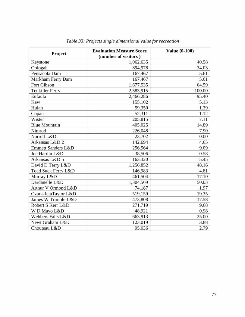
77

Table 33: Projects single dimensional value for recreation


(number of visitors )

Value (0-100)

Keystone 1,062,635 40.58

Oologah 894,978 34.03


Markham Ferry Dam 167,467 5.61

Fort Gibson 1,677,535 64.59

Tenkiller Ferry 2,583,915 100.00

Eufaula 2,466,286 95.40

Kaw 155,102 5.13

Hulah 59,350 1.39

Copan 52,311 1.12

Wister 205,815 7.11

Blue Mountain 405,025 14.89

Nimrod 226,048 7.90

Norrell L&D 23,702 0.00

Arkansas L&D 2 142,694 4.65

Emmett Sanders L&D 256,564 9.09

Joe Hardin L&D 38,506 0.58

Arkansas L&D 5 163,320 5.45

David D Terry L&D 1,256,852 48.16

Toad Suck Ferry L&D 146,983 4.81

Murray L&D 461,504 17.10

Dardanelle L&D 1,304,569 50.03

Arthur V Ormond L&D 74,187 1.97

Ozark-JetaTaylor L&D 519,159 19.35

James W Trimble L&D 473,808 17.58

Robert S Kerr L&D 271,719 9.68

W D Mayo L&D 48,921 0.98

Webbers Falls L&D 663,913 25.00

Newt Graham L&D 123,019 3.88

Chouteau L&D 95,036 2.79

78

Appendix B: One way Sensitivity Analysis Results

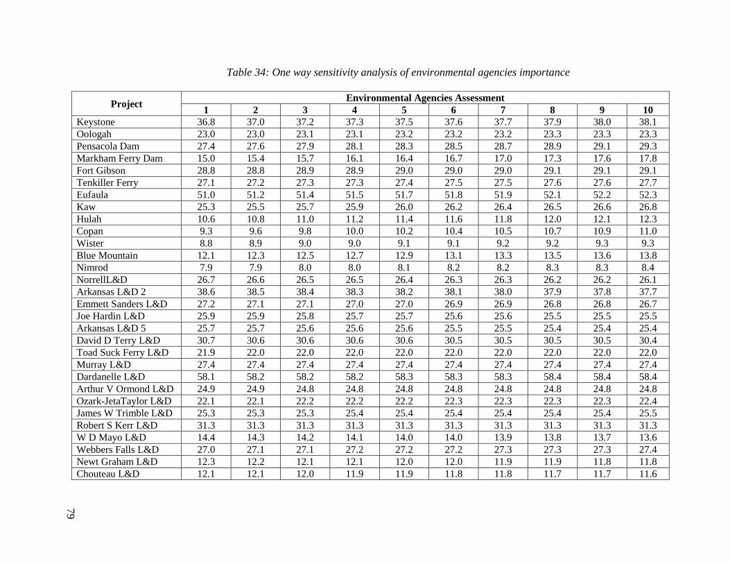
79

Table 34: One way sensitivity analysis of environmental agencies importance

Project Environmental Agencies Assessment

1 2 3 4 5 6 7 8 9 10

Keystone 36.8 37.0 37.2 37.3 37.5 37.6 37.7 37.9 38.0 38.1

Oologah 23.0 23.0 23.1 23.1 23.2 23.2 23.2 23.3 23.3 23.3

Pensacola Dam 27.4 27.6 27.9 28.1 28.3 28.5 28.7 28.9 29.1 29.3

Markham Ferry Dam 15.0 15.4 15.7 16.1 16.4 16.7 17.0 17.3 17.6 17.8

Fort Gibson 28.8 28.8 28.9 28.9 29.0 29.0 29.0 29.1 29.1 29.1

Tenkiller Ferry 27.1 27.2 27.3 27.3 27.4 27.5 27.5 27.6 27.6 27.7

Eufaula 51.0 51.2 51.4 51.5 51.7 51.8 51.9 52.1 52.2 52.3

Kaw 25.3 25.5 25.7 25.9 26.0 26.2 26.4 26.5 26.6 26.8

Hulah 10.6 10.8 11.0 11.2 11.4 11.6 11.8 12.0 12.1 12.3

Copan 9.3 9.6 9.8 10.0 10.2 10.4 10.5 10.7 10.9 11.0

Wister 8.8 8.9 9.0 9.0 9.1 9.1 9.2 9.2 9.3 9.3

Blue Mountain 12.1 12.3 12.5 12.7 12.9 13.1 13.3 13.5 13.6 13.8

Nimrod 7.9 7.9 8.0 8.0 8.1 8.2 8.2 8.3 8.3 8.4

NorrellL&D 26.7 26.6 26.5 26.5 26.4 26.3 26.3 26.2 26.2 26.1

Arkansas L&D 2 38.6 38.5 38.4 38.3 38.2 38.1 38.0 37.9 37.8 37.7

Emmett Sanders L&D 27.2 27.1 27.1 27.0 27.0 26.9 26.9 26.8 26.8 26.7

Joe Hardin L&D 25.9 25.9 25.8 25.7 25.7 25.6 25.6 25.5 25.5 25.5

Arkansas L&D 5 25.7 25.7 25.6 25.6 25.6 25.5 25.5 25.4 25.4 25.4

David D Terry L&D 30.7 30.6 30.6 30.6 30.6 30.5 30.5 30.5 30.5 30.4

Toad Suck Ferry L&D 21.9 22.0 22.0 22.0 22.0 22.0 22.0 22.0 22.0 22.0

Murray L&D 27.4 27.4 27.4 27.4 27.4 27.4 27.4 27.4 27.4 27.4

Dardanelle L&D 58.1 58.2 58.2 58.2 58.3 58.3 58.3 58.4 58.4 58.4

Arthur V Ormond L&D 24.9 24.9 24.8 24.8 24.8 24.8 24.8 24.8 24.8 24.8

Ozark-JetaTaylor L&D 22.1 22.1 22.2 22.2 22.2 22.3 22.3 22.3 22.3 22.4

James W Trimble L&D 25.3 25.3 25.3 25.4 25.4 25.4 25.4 25.4 25.4 25.5

Robert S Kerr L&D 31.3 31.3 31.3 31.3 31.3 31.3 31.3 31.3 31.3 31.3

W D Mayo L&D 14.4 14.3 14.2 14.1 14.0 14.0 13.9 13.8 13.7 13.6

Webbers Falls L&D 27.0 27.1 27.1 27.2 27.2 27.2 27.3 27.3 27.3 27.4

Newt Graham L&D 12.3 12.2 12.1 12.1 12.0 12.0 11.9 11.9 11.8 11.8

Chouteau L&D 12.1 12.1 12.0 11.9 11.9 11.8 11.8 11.7 11.7 11.6

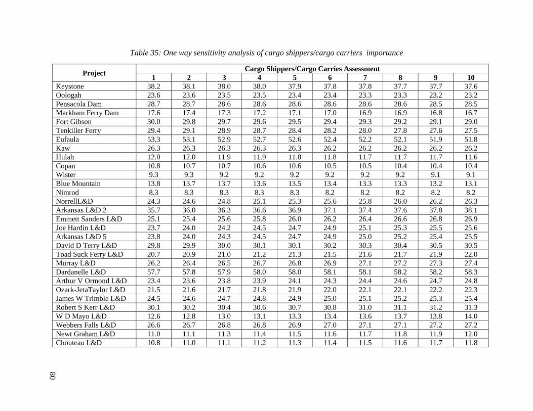
80

Table 35: One way sensitivity analysis of cargo shippers/cargo carriers importance

Project Cargo Shippers/Cargo Carries Assessment

1 2 3 4 5 6 7 8 9 10

Keystone 38.2 38.1 38.0 38.0 37.9 37.8 37.8 37.7 37.7 37.6

Oologah 23.6 23.6 23.5 23.5 23.4 23.4 23.3 23.3 23.2 23.2

Pensacola Dam 28.7 28.7 28.6 28.6 28.6 28.6 28.6 28.6 28.5 28.5


Fort Gibson 30.0 29.8 29.7 29.6 29.5 29.4 29.3 29.2 29.1 29.0

Tenkiller Ferry 29.4 29.1 28.9 28.7 28.4 28.2 28.0 27.8 27.6 27.5

Eufaula 53.3 53.1 52.9 52.7 52.6 52.4 52.2 52.1 51.9 51.8

Kaw 26.3 26.3 26.3 26.3 26.3 26.2 26.2 26.2 26.2 26.2

Hulah 12.0 12.0 11.9 11.9 11.8 11.8 11.7 11.7 11.7 11.6

Copan 10.8 10.7 10.7 10.6 10.6 10.5 10.5 10.4 10.4 10.4

Wister 9.3 9.3 9.2 9.2 9.2 9.2 9.2 9.2 9.1 9.1

Blue Mountain 13.8 13.7 13.7 13.6 13.5 13.4 13.3 13.3 13.2 13.1

Nimrod 8.3 8.3 8.3 8.3 8.3 8.2 8.2 8.2 8.2 8.2

NorrellL&D 24.3 24.6 24.8 25.1 25.3 25.6 25.8 26.0 26.2 26.3

Arkansas L&D 2 35.7 36.0 36.3 36.6 36.9 37.1 37.4 37.6 37.8 38.1


Joe Hardin L&D 23.7 24.0 24.2 24.5 24.7 24.9 25.1 25.3 25.5 25.6

Arkansas L&D 5 23.8 24.0 24.3 24.5 24.7 24.9 25.0 25.2 25.4 25.5

David D Terry L&D 29.8 29.9 30.0 30.1 30.1 30.2 30.3 30.4 30.5 30.5


Murray L&D 26.2 26.4 26.5 26.7 26.8 26.9 27.1 27.2 27.3 27.4

Dardanelle L&D 57.7 57.8 57.9 58.0 58.0 58.1 58.1 58.2 58.2 58.3




Robert S Kerr L&D 30.1 30.2 30.4 30.6 30.7 30.8 31.0 31.1 31.2 31.3

W D Mayo L&D 12.6 12.8 13.0 13.1 13.3 13.4 13.6 13.7 13.8 14.0

Webbers Falls L&D 26.6 26.7 26.8 26.8 26.9 27.0 27.1 27.1 27.2 27.2

Newt Graham L&D 11.0 11.1 11.3 11.4 11.5 11.6 11.7 11.8 11.9 12.0

Chouteau L&D 10.8 11.0 11.1 11.2 11.3 11.4 11.5 11.6 11.7 11.8

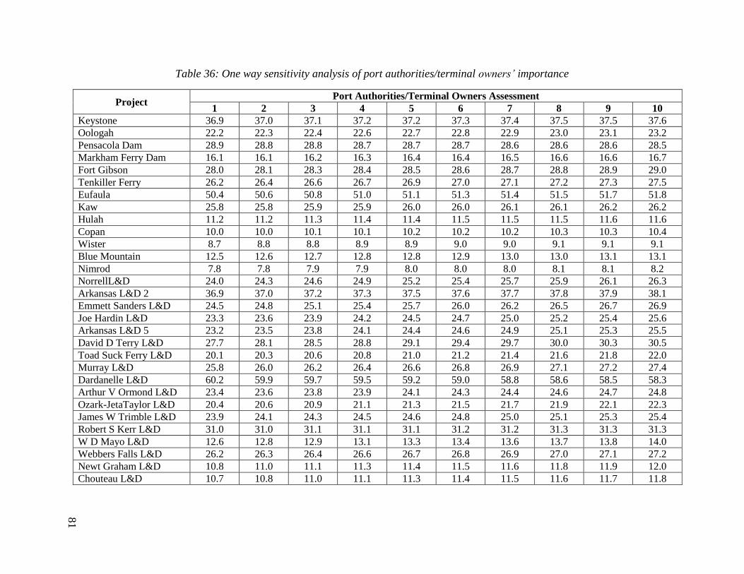
81

Table 36: One way sensitivity analysis of port authorities/terminal owners’ importance

Project Port Authorities/Terminal Owners Assessment

1 2 3 4 5 6 7 8 9 10

Keystone 36.9 37.0 37.1 37.2 37.2 37.3 37.4 37.5 37.5 37.6

Oologah 22.2 22.3 22.4 22.6 22.7 22.8 22.9 23.0 23.1 23.2

Pensacola Dam 28.9 28.8 28.8 28.7 28.7 28.7 28.6 28.6 28.6 28.5


Fort Gibson 28.0 28.1 28.3 28.4 28.5 28.6 28.7 28.8 28.9 29.0

Tenkiller Ferry 26.2 26.4 26.6 26.7 26.9 27.0 27.1 27.2 27.3 27.5

Eufaula 50.4 50.6 50.8 51.0 51.1 51.3 51.4 51.5 51.7 51.8

Kaw 25.8 25.8 25.9 25.9 26.0 26.0 26.1 26.1 26.2 26.2

Hulah 11.2 11.2 11.3 11.4 11.4 11.5 11.5 11.5 11.6 11.6

Copan 10.0 10.0 10.1 10.1 10.2 10.2 10.2 10.3 10.3 10.4

Wister 8.7 8.8 8.8 8.9 8.9 9.0 9.0 9.1 9.1 9.1

Blue Mountain 12.5 12.6 12.7 12.8 12.8 12.9 13.0 13.0 13.1 13.1

Nimrod 7.8 7.8 7.9 7.9 8.0 8.0 8.0 8.1 8.1 8.2

NorrellL&D 24.0 24.3 24.6 24.9 25.2 25.4 25.7 25.9 26.1 26.3

Arkansas L&D 2 36.9 37.0 37.2 37.3 37.5 37.6 37.7 37.8 37.9 38.1


Joe Hardin L&D 23.3 23.6 23.9 24.2 24.5 24.7 25.0 25.2 25.4 25.6

Arkansas L&D 5 23.2 23.5 23.8 24.1 24.4 24.6 24.9 25.1 25.3 25.5

David D Terry L&D 27.7 28.1 28.5 28.8 29.1 29.4 29.7 30.0 30.3 30.5


Murray L&D 25.8 26.0 26.2 26.4 26.6 26.8 26.9 27.1 27.2 27.4

Dardanelle L&D 60.2 59.9 59.7 59.5 59.2 59.0 58.8 58.6 58.5 58.3




Robert S Kerr L&D 31.0 31.0 31.1 31.1 31.1 31.2 31.2 31.3 31.3 31.3

W D Mayo L&D 12.6 12.8 12.9 13.1 13.3 13.4 13.6 13.7 13.8 14.0

Webbers Falls L&D 26.2 26.3 26.4 26.6 26.7 26.8 26.9 27.0 27.1 27.2

Newt Graham L&D 10.8 11.0 11.1 11.3 11.4 11.5 11.6 11.8 11.9 12.0

Chouteau L&D 10.7 10.8 11.0 11.1 11.3 11.4 11.5 11.6 11.7 11.8

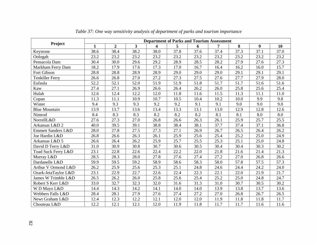
82

Table 37: One way sensitivity analysis of department of parks and tourism importance

Project Department of Parks and Tourism Assessment

1 2 3 4 5 6 7 8 9 10

Keystone 38.6 38.4 38.2 38.0 37.8 37.6 37.4 37.3 37.1 37.0

Oologah 23.2 23.2 23.2 23.2 23.2 23.2 23.2 23.2 23.2 23.2

Pensacola Dam 30.4 30.0 29.6 29.2 28.9 28.5 28.2 27.9 27.6 27.3


Fort Gibson 28.8 28.8 28.9 28.9 29.0 29.0 29.0 29.1 29.1 29.1

Tenkiller Ferry 26.6 26.8 27.0 27.2 27.3 27.5 27.6 27.7 27.9 28.0

Eufaula 52.2 52.1 52.0 51.9 51.9 51.8 51.7 51.7 51.6 51.6

Kaw 27.4 27.1 26.9 26.6 26.4 26.2 26.0 25.8 25.6 25.4

Hulah 12.6 12.4 12.2 12.0 11.8 11.6 11.5 11.3 11.1 11.0

Copan 11.3 11.1 10.9 10.7 10.5 10.4 10.2 10.0 9.9 9.8

Wister 9.4 9.3 9.3 9.2 9.2 9.1 9.1 9.0 9.0 9.0

Blue Mountain 13.9 13.7 13.6 13.4 13.3 13.1 13.0 12.9 12.8 12.6

Nimrod 8.4 8.3 8.3 8.2 8.2 8.2 8.1 8.1 8.0 8.0

NorrellL&D 27.6 27.3 27.0 26.8 26.6 26.3 26.1 25.9 25.7 25.5

Arkansas L&D 2 40.0 39.5 39.1 38.8 38.4 38.1 37.7 37.4 37.1 36.8


Joe Hardin L&D 26.8 26.6 26.3 26.1 25.9 25.6 25.4 25.2 25.0 24.9

Arkansas L&D 5 26.6 26.4 26.2 25.9 25.7 25.5 25.3 25.1 25.0 24.8

David D Terry L&D 31.0 30.9 30.8 30.7 30.6 30.5 30.4 30.4 30.3 30.2


Murray L&D 28.5 28.3 28.0 27.8 27.6 27.4 27.2 27.0 26.8 26.6

Dardanelle L&D 59.9 59.5 59.2 58.9 58.6 58.3 58.0 57.8 57.5 57.3




Robert S Kerr L&D 33.0 32.7 32.3 32.0 31.6 31.3 31.0 30.7 30.5 30.2

W D Mayo L&D 14.4 14.3 14.2 14.1 14.0 14.0 13.9 13.8 13.7 13.6

Webbers Falls L&D 28.4 28.1 27.9 27.6 27.4 27.2 27.0 26.8 26.7 26.5

Newt Graham L&D 12.4 12.3 12.2 12.1 12.0 12.0 11.9 11.8 11.8 11.7

Chouteau L&D 12.2 12.1 12.1 12.0 11.9 11.8 11.7 11.7 11.6 11.6

83

Table 38: One way sensitivity analysis of utility companies’ importance

Project Utility Companies Assessment

1 2 3 4 5 6 7 8 9 10

Keystone 37.8 37.8 37.7 37.7 37.7 37.7 37.6 37.6 37.6 37.6

Oologah 24.3 24.1 24.0 23.8 23.7 23.6 23.4 23.3 23.2 23.1

Pensacola Dam 27.1 27.3 27.5 27.7 27.9 28.1 28.2 28.4 28.5 28.7


Fort Gibson 30.0 29.9 29.7 29.6 29.5 29.3 29.2 29.1 29.0 28.9

Tenkiller Ferry 29.0 28.8 28.6 28.4 28.2 28.0 27.8 27.6 27.5 27.3

Eufaula 52.9 52.7 52.6 52.4 52.3 52.2 52.0 51.9 51.8 51.7

Kaw 26.1 26.1 26.1 26.1 26.2 26.2 26.2 26.2 26.2 26.2

Hulah 11.6 11.6 11.6 11.6 11.6 11.6 11.6 11.6 11.6 11.6

Copan 10.3 10.3 10.3 10.3 10.3 10.4 10.4 10.4 10.4 10.4

Wister 9.4 9.4 9.3 9.3 9.3 9.2 9.2 9.2 9.1 9.1

Blue Mountain 13.4 13.4 13.3 13.3 13.3 13.2 13.2 13.2 13.1 13.1

Nimrod 8.5 8.4 8.4 8.3 8.3 8.3 8.2 8.2 8.2 8.1

NorrellL&D 28.0 27.7 27.5 27.3 27.1 26.9 26.7 26.5 26.3 26.2

Arkansas L&D 2 37.9 37.9 38.0 38.0 38.0 38.0 38.0 38.0 38.1 38.1


Joe Hardin L&D 27.2 27.0 26.8 26.5 26.3 26.2 26.0 25.8 25.6 25.5

Arkansas L&D 5 27.1 26.9 26.7 26.4 26.2 26.0 25.9 25.7 25.5 25.4

David D Terry L&D 33.0 32.6 32.3 31.9 31.6 31.3 31.0 30.8 30.5 30.3


Murray L&D 28.2 28.1 28.0 27.9 27.7 27.7 27.6 27.5 27.4 27.3

Dardanelle L&D 55.5 55.9 56.3 56.7 57.0 57.4 57.7 58.0 58.3 58.6




Robert S Kerr L&D 30.5 30.7 30.8 30.9 31.0 31.1 31.2 31.2 31.3 31.4

W D Mayo L&D 15.0 14.8 14.7 14.6 14.4 14.3 14.2 14.1 14.0 13.8

Webbers Falls L&D 27.5 27.5 27.4 27.4 27.4 27.3 27.3 27.3 27.2 27.2

Newt Graham L&D 12.8 12.7 12.6 12.5 12.4 12.3 12.2 12.1 12.0 11.9

Chouteau L&D 12.7 12.5 12.4 12.3 12.2 12.1 12.0 11.9 11.8 11.7

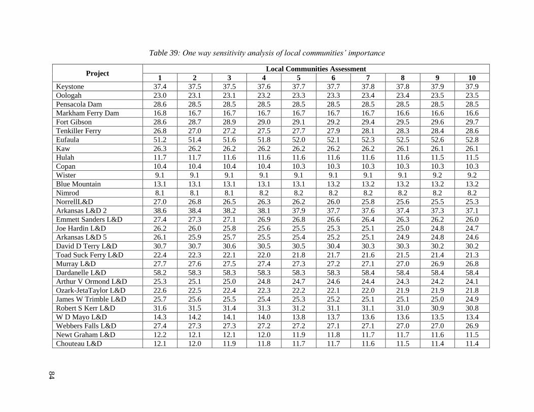
84

Table 39: One way sensitivity analysis of local communities’ importance

Project Local Communities Assessment

1 2 3 4 5 6 7 8 9 10

Keystone 37.4 37.5 37.5 37.6 37.7 37.7 37.8 37.8 37.9 37.9

Oologah 23.0 23.1 23.1 23.2 23.3 23.3 23.4 23.4 23.5 23.5

Pensacola Dam 28.6 28.5 28.5 28.5 28.5 28.5 28.5 28.5 28.5 28.5


Fort Gibson 28.6 28.7 28.9 29.0 29.1 29.2 29.4 29.5 29.6 29.7

Tenkiller Ferry 26.8 27.0 27.2 27.5 27.7 27.9 28.1 28.3 28.4 28.6

Eufaula 51.2 51.4 51.6 51.8 52.0 52.1 52.3 52.5 52.6 52.8

Kaw 26.3 26.2 26.2 26.2 26.2 26.2 26.2 26.1 26.1 26.1

Hulah 11.7 11.7 11.6 11.6 11.6 11.6 11.6 11.6 11.5 11.5

Copan 10.4 10.4 10.4 10.4 10.3 10.3 10.3 10.3 10.3 10.3

Wister 9.1 9.1 9.1 9.1 9.1 9.1 9.1 9.1 9.2 9.2

Blue Mountain 13.1 13.1 13.1 13.1 13.1 13.2 13.2 13.2 13.2 13.2

Nimrod 8.1 8.1 8.1 8.2 8.2 8.2 8.2 8.2 8.2 8.2

NorrellL&D 27.0 26.8 26.5 26.3 26.2 26.0 25.8 25.6 25.5 25.3

Arkansas L&D 2 38.6 38.4 38.2 38.1 37.9 37.7 37.6 37.4 37.3 37.1


Joe Hardin L&D 26.2 26.0 25.8 25.6 25.5 25.3 25.1 25.0 24.8 24.7

Arkansas L&D 5 26.1 25.9 25.7 25.5 25.4 25.2 25.1 24.9 24.8 24.6

David D Terry L&D 30.7 30.7 30.6 30.5 30.5 30.4 30.3 30.3 30.2 30.2


Murray L&D 27.7 27.6 27.5 27.4 27.3 27.2 27.1 27.0 26.9 26.8

Dardanelle L&D 58.2 58.3 58.3 58.3 58.3 58.3 58.4 58.4 58.4 58.4




Robert S Kerr L&D 31.6 31.5 31.4 31.3 31.2 31.1 31.1 31.0 30.9 30.8

W D Mayo L&D 14.3 14.2 14.1 14.0 13.8 13.7 13.6 13.6 13.5 13.4

Webbers Falls L&D 27.4 27.3 27.3 27.2 27.2 27.1 27.1 27.0 27.0 26.9

Newt Graham L&D 12.2 12.1 12.1 12.0 11.9 11.8 11.7 11.7 11.6 11.5

Chouteau L&D 12.1 12.0 11.9 11.8 11.7 11.7 11.6 11.5 11.4 11.4

Documents

Othman Boudhoum Thesis