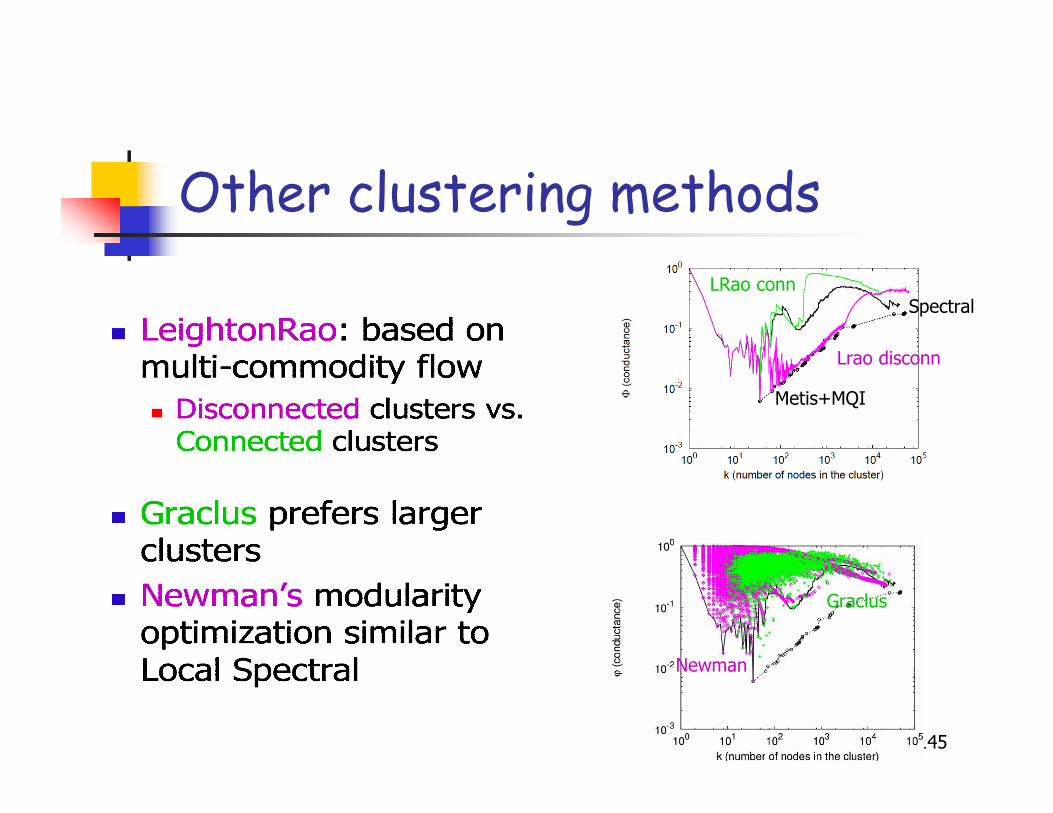
Other clustering methods

145

Spectral

Metis+MQI

Lrao disconn

LRao conn

Newman

Graclus

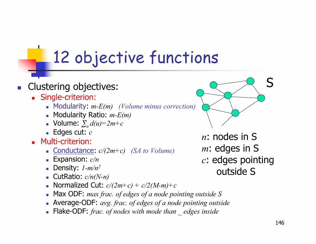
12 objective functions Clustering objectives:

Single-criterion: Modularity: m-E(m) (Volume minus correction) Modularity Ratio: m-E(m) Volume: ∑u d(u)=2m+c Edges cut: c

Multi-criterion: Conductance: c/(2m+c) (SA to Volume) Expansion: c/n Density: 1-m/n2

CutRatio: c/n(N-n) Normalized Cut: c/(2m+c) + c/2(M-m)+c Max ODF: max frac. of edges of a node pointing outside S Average-ODF: avg. frac. of edges of a node pointing outside Flake-ODF: frac. of nodes with mode than _ edges inside

146

S

n: nodes in Sm: edges in Sc: edges pointing outside S

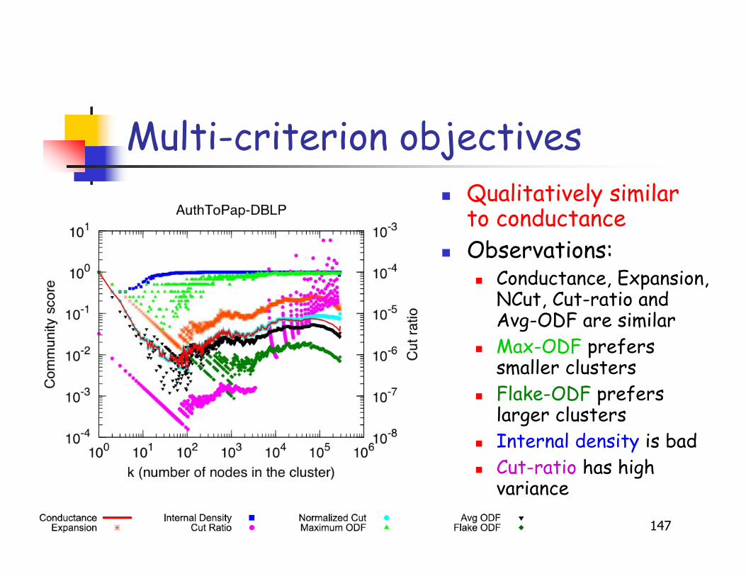
Multi-criterion objectives

147

Qualitatively similarto conductance

Observations: Conductance, Expansion,

NCut, Cut-ratio andAvg-ODF are similar

Max-ODF preferssmaller clusters

Flake-ODF preferslarger clusters

Internal density is bad Cut-ratio has high

variance

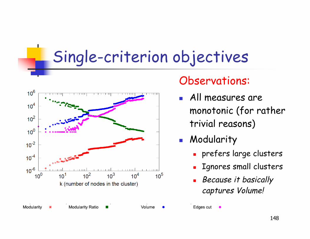
Single-criterion objectives

148

Observations: All measures are

monotonic (for rathertrivial reasons)

Modularity prefers large clusters Ignores small clusters Because it basically

captures Volume!

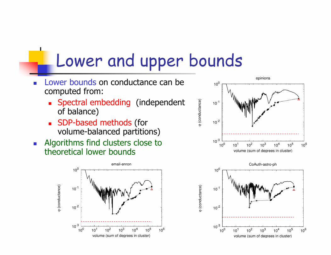
Lower and upper bounds Lower bounds on conductance can be

computed from: Spectral embedding (independent

of balance) SDP-based methods (for

volume-balanced partitions) Algorithms find clusters close to

theoretical lower bounds

149

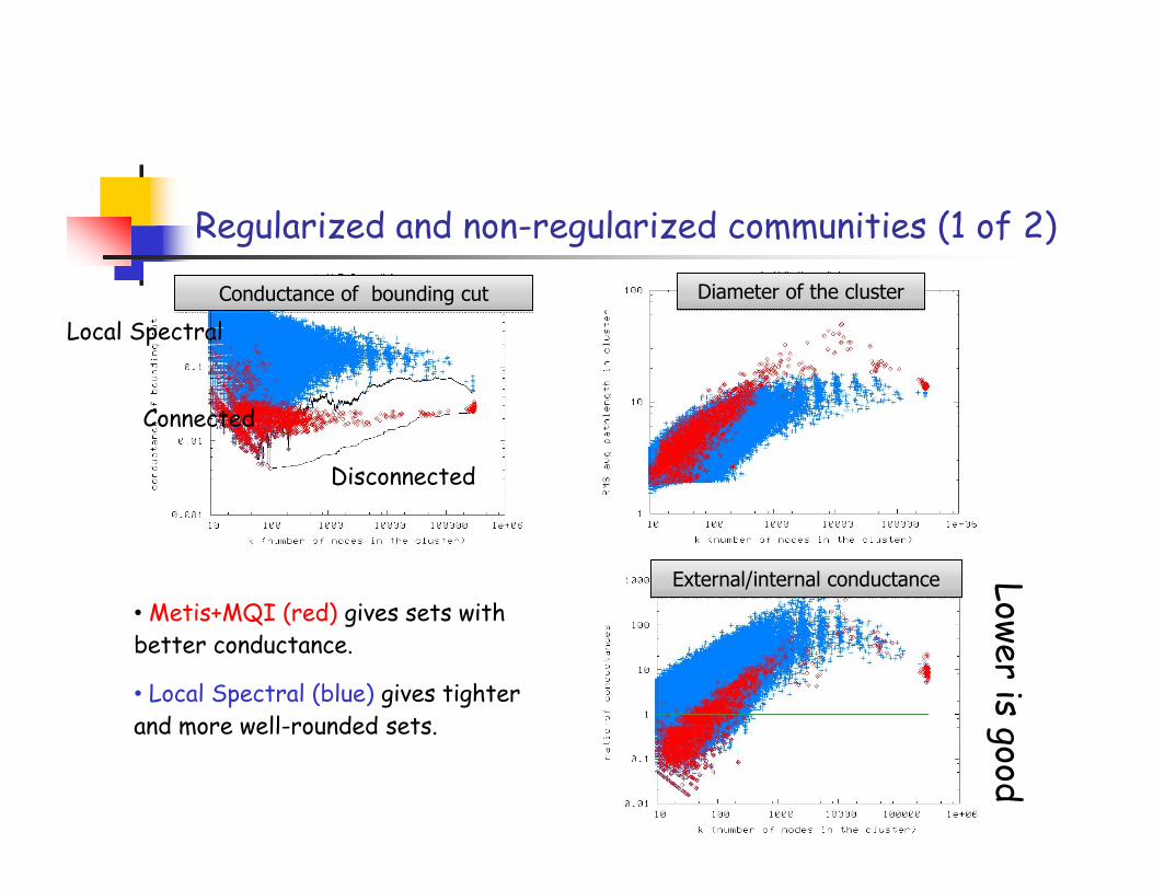
Regularized and non-regularized communities (1 of 2)

• Metis+MQI (red) gives sets withbetter conductance.

• Local Spectral (blue) gives tighterand more well-rounded sets.

External/internal conductanceExternal/internal conductance

Diameter of the clusterDiameter of the clusterConductance of bounding cutConductance of bounding cut

Local Spectral

Connected

Disconnected

Lower is good

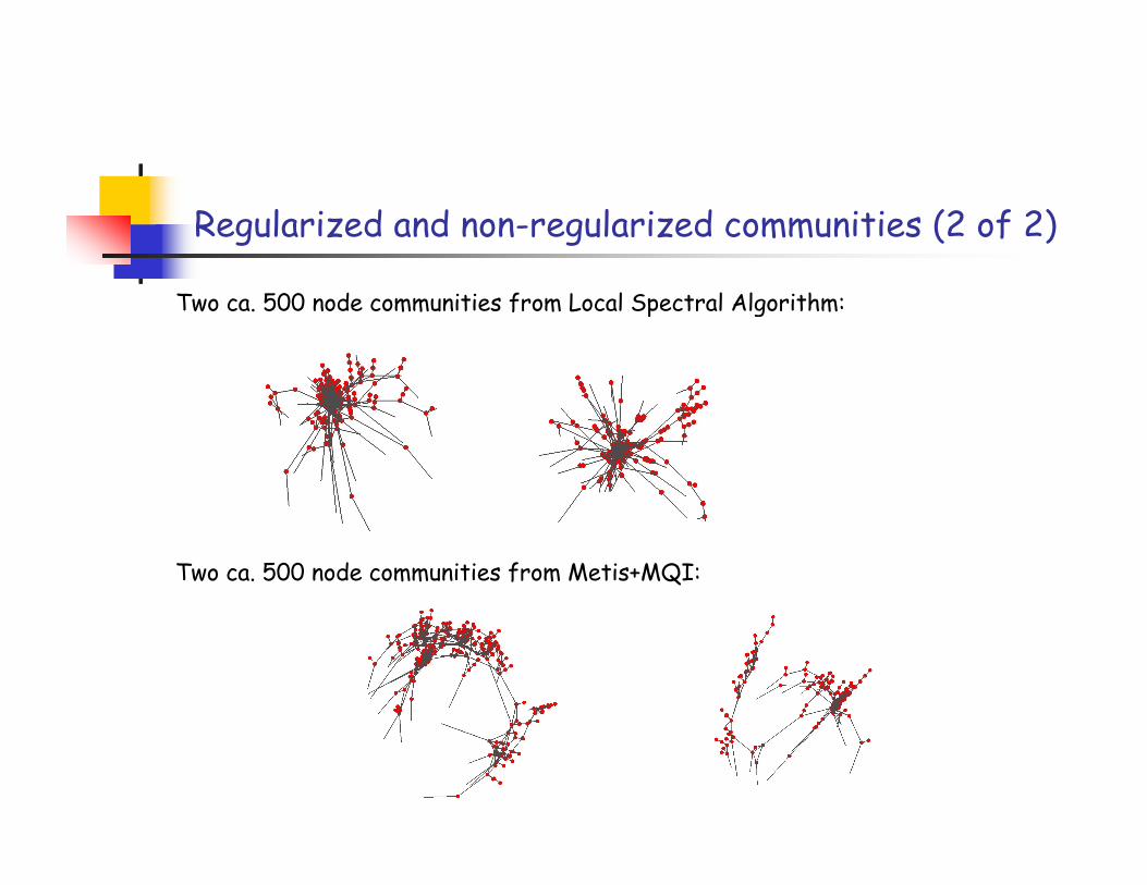
Regularized and non-regularized communities (2 of 2)

Two ca. 500 node communities from Local Spectral Algorithm:

Two ca. 500 node communities from Metis+MQI:

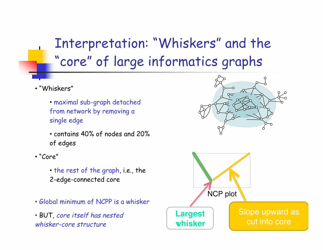
Interpretation: “Whiskers” and the“core” of large informatics graphs

• “Whiskers”

• maximal sub-graph detachedfrom network by removing asingle edge

• contains 40% of nodes and 20%of edges

• “Core”

• the rest of the graph, i.e., the2-edge-connected core

• Global minimum of NCPP is a whisker

• BUT, core itself has nestedwhisker-core structure

NCP plot

Largestwhisker

Slope upward ascut into core

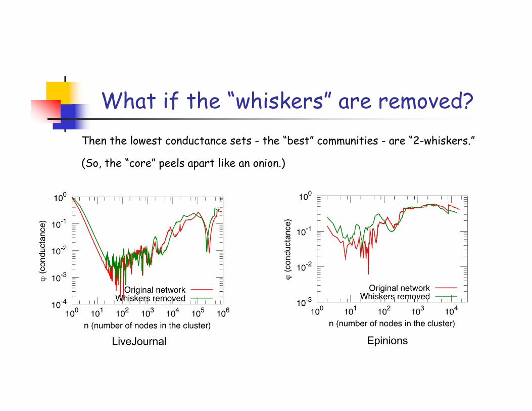
What if the “whiskers” are removed?

LiveJournal Epinions

Then the lowest conductance sets - the “best” communities - are “2-whiskers.”

(So, the “core” peels apart like an onion.)

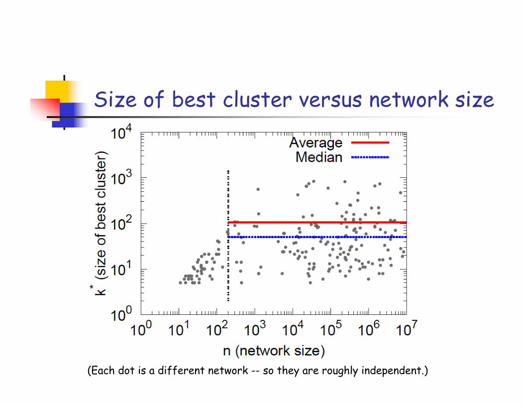
Size of best cluster versus network size

(Each dot is a different network -- so they are roughly independent.)

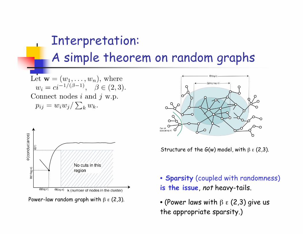
Interpretation:A simple theorem on random graphs

Power-law random graph with β ε (2,3).

Structure of the G(w) model, with β ε (2,3).

• Sparsity (coupled with randomness)is the issue, not heavy-tails.

• (Power laws with β ε (2,3) give usthe appropriate sparsity.)

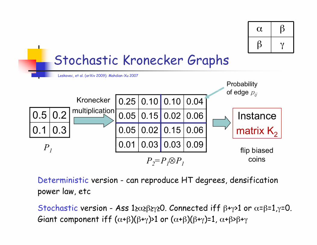
Stochastic Kronecker Graphs

Deterministic version - can reproduce HT degrees, densificationpower law, etc

Stochastic version - Ass 1≥α≥β≥γ≥0. Connected iff β+γ>1 or α=β=1,γ=0.Giant component iff (α+β)(β+γ)>1 or (α+β)(β+γ)=1, α+β>β+γ

Leskovec, et al. (arXiv 2009); Mahdian-Xu 2007

α β

β γ

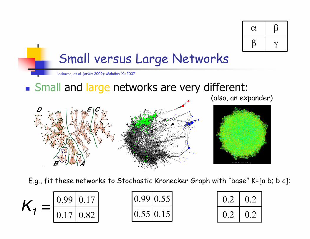
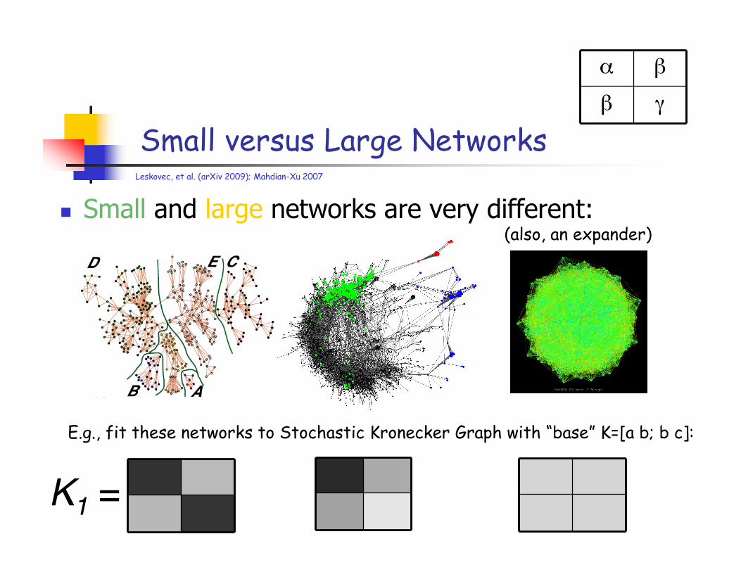
Small versus Large NetworksLeskovec, et al. (arXiv 2009); Mahdian-Xu 2007

Small and large networks are very different:

0.99 0.55

0.55 0.15

0.99 0.17

0.17 0.82K1 =

E.g., fit these networks to Stochastic Kronecker Graph with “base” K=[a b; b c]:

α β

β γ

0.2 0.2

0.2 0.2

(also, an expander)

Small versus Large NetworksLeskovec, et al. (arXiv 2009); Mahdian-Xu 2007

Small and large networks are very different:

K1 =E.g., fit these networks to Stochastic Kronecker Graph with “base” K=[a b; b c]:

α β

β γ

(also, an expander)

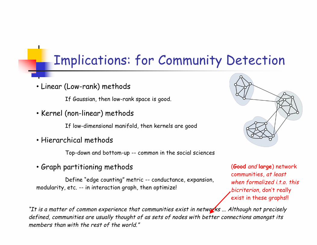
Implications: for Community Detection

• Linear (Low-rank) methodsIf Gaussian, then low-rank space is good.

• Kernel (non-linear) methodsIf low-dimensional manifold, then kernels are good

• Hierarchical methodsTop-down and bottom-up -- common in the social sciences

• Graph partitioning methodsDefine “edge counting” metric -- conductance, expansion,

modularity, etc. -- in interaction graph, then optimize!

“It is a matter of common experience that communities exist in networks ... Although not preciselydefined, communities are usually thought of as sets of nodes with better connections amongst itsmembers than with the rest of the world.”

(Good and large) networkcommunities, at leastwhen formalized i.t.o. thisbicriterion, don’t reallyexist in these graphs!!

Comparison with “Ground truth” (1 of 2)

Networks with “ground truth” communities:

• LiveJournal12:• users create and explicitly join on-line groups

• CA-DBLP:• publication venues can be viewed as communities

• AmazonAllProd:• each item belongs to one or more hierarchically organizedcategories, as defined by Amazon

• AtM-IMDB:• countries of production and languages may be viewed ascommunities (thus every movie belongs to exactly onecommunity and actors belongs to all communities to whichmovies in which they appeared belong)

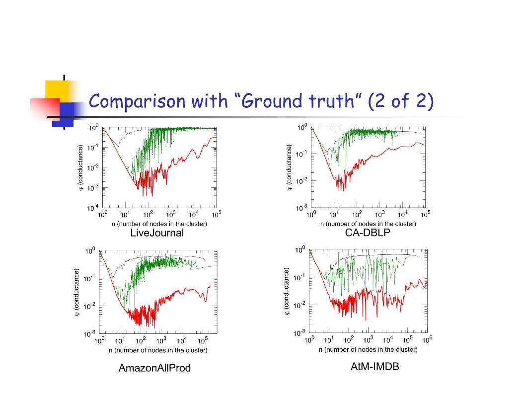
Comparison with “Ground truth” (2 of 2)

LiveJournal CA-DBLP

AmazonAllProd AtM-IMDB

Miscellaneous thoughts ...

Sociological work on community size (Dunbar and Allen)• 150 individuals is maximum community size• Military companies, on-line communities, divisions of corporations all ≤ 150

Common bond vs. common identity theory• Common bond - people are attached to individual community members• Common identity - people are attached to the group as a whole

What edges “mean” and community identification• social networks - reasons an individual adds a link to a friend very diverse• citation networks - links are more “expensive” and semantically uniform.

Implications: high level

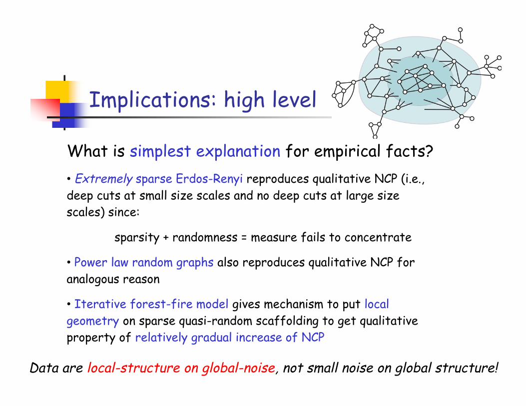
What is simplest explanation for empirical facts?• Extremely sparse Erdos-Renyi reproduces qualitative NCP (i.e.,deep cuts at small size scales and no deep cuts at large sizescales) since:

sparsity + randomness = measure fails to concentrate

• Power law random graphs also reproduces qualitative NCP foranalogous reason

• Iterative forest-fire model gives mechanism to put localgeometry on sparse quasi-random scaffolding to get qualitativeproperty of relatively gradual increase of NCP

Data are local-structure on global-noise, not small noise on global structure!

Implications: high level, cont.

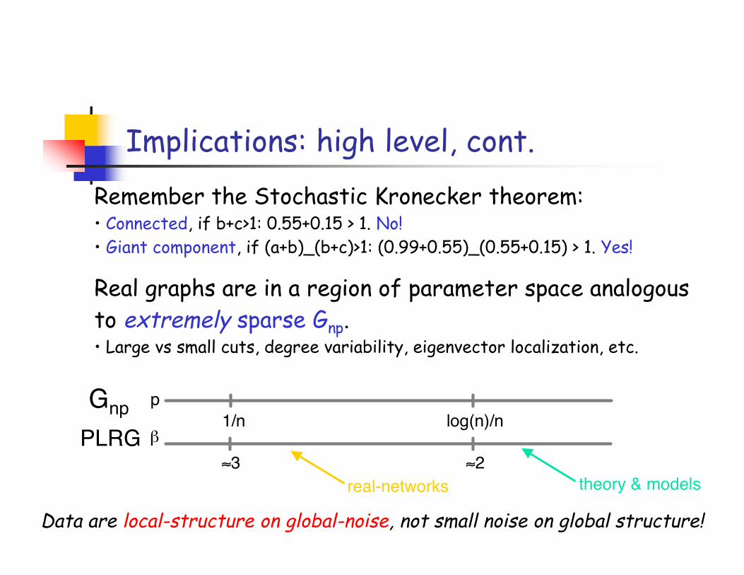
Remember the Stochastic Kronecker theorem:• Connected, if b+c>1: 0.55+0.15 > 1. No!• Giant component, if (a+b)_(b+c)>1: (0.99+0.55)_(0.55+0.15) > 1. Yes!

Real graphs are in a region of parameter space analogousto extremely sparse Gnp.• Large vs small cuts, degree variability, eigenvector localization, etc.

1/nGnp log(n)/n

real-networks theory & models≈3

PLRG≈2

p

β

Data are local-structure on global-noise, not small noise on global structure!

Degree heterogeneity and hyperbolicity

Social and information networks are expander-like atlarge size scales, but:

• Degree heterogeneity enhances hyperbolicity

Lots of evidence:• Scale free and internet graphs are more hyperbolic than other models, MC simulation -Jonckheere and Lohsoonthorne (2007)

• Mapping network nodes to spaces of negative curvature leads to scale-free structure -Krioukov et al (2008)

• Measurements of Internet are Gromov negatively curved - Baryshnikov (2002)

• Curvature of co-links interpreted as thematic layers in WWW - Eckmann and Moses (2002)

Question: Has anyone made this observation precise?

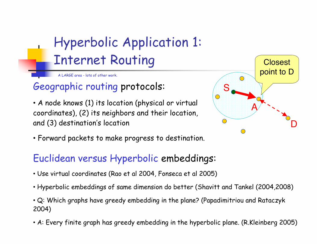
Hyperbolic Application 1:Internet Routing

Geographic routing protocols:• A node knows (1) its location (physical or virtualcoordinates), (2) its neighbors and their location,and (3) destination’s location

• Forward packets to make progress to destination.

A LARGE area - lots of other work.

Euclidean versus Hyperbolic embeddings:• Use virtual coordinates (Rao et al 2004, Fonseca et al 2005)

• Hyperbolic embeddings of same dimension do better (Shavitt and Tankel (2004,2008)

• Q: Which graphs have greedy embedding in the plane? (Papadimitriou and Rataczyk2004)

• A: Every finite graph has greedy embedding in the hyperbolic plane. (R.Kleinberg 2005)

S

DA

Closestpoint to D

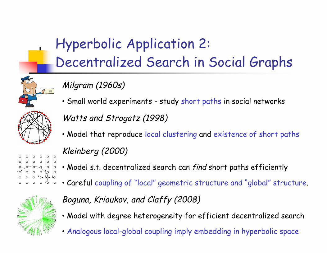
Hyperbolic Application 2:Decentralized Search in Social Graphs

Milgram (1960s)

• Small world experiments - study short paths in social networks

Watts and Strogatz (1998)

• Model that reproduce local clustering and existence of short paths

Kleinberg (2000)

• Model s.t. decentralized search can find short paths efficiently

• Careful coupling of “local” geometric structure and “global” structure.

Boguna, Krioukov, and Claffy (2008)

• Model with degree heterogeneity for efficient decentralized search

• Analogous local-global coupling imply embedding in hyperbolic space

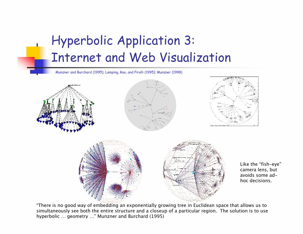
Hyperbolic Application 3:Internet and Web Visualization

Munzner and Burchard (1995); Lamping, Rao, and Pirolli (1995); Munzner (1998)

“There is no good way of embedding an exponentially growing tree in Euclidean space that allows us tosimultaneously see both the entire structure and a closeup of a particular region. The solution is to usehyperbolic … geometry …” Munzner and Burchard (1995)

Like the “fish-eye”camera lens, butavoids some ad-hoc decisions.

“Routing” versus “diffusion” metrics

Consider two classes of “distances” between nodes:

• “Diffusion-type” distance - related to (spectral methods and)diffusion or commute times

• “Geodesic-type” distance - related to (flow-based methods and)routing or shortest paths

Question 1: Which is better? More useful? (As afunction of the type of graph)?

Question 2: Given that a process goes from A to Bwith one of those processes, how does the pathcompare with the other process?

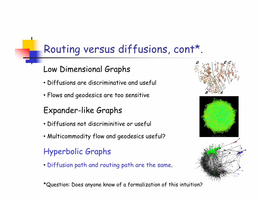
Routing versus diffusions, cont*.

Low Dimensional Graphs• Diffusions are discriminative and useful

• Flows and geodesics are too sensitive

Expander-like Graphs• Diffusions not discriminitive or useful

• Multicommodity flow and geodesics useful?

Hyperbolic Graphs• Diffusion path and routing path are the same.

*Question: Does anyone know of a formalization of this intuition?

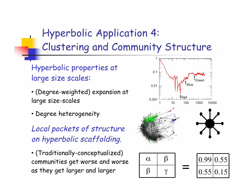
Hyperbolic Application 4:Clustering and Community Structure

Hyperbolic properties atlarge size scales:

• (Degree-weighted) expansion atlarge size-scales

• Degree heterogeneity

Local pockets of structureon hyperbolic scaffolding.

• (Traditionally-conceptualized)communities get worse and worseas they get larger and larger

α β

β γ

0.99 0.55

0.55 0.15=

Implications for Data Analysis and ML

Principled and scalable algorithmic exploratory analysis tools:

• spectral vs. flow vs. combinations; local vs. global vs. improvement; etc.

Doing inference directly on data graphs, and machine learning incomplex data environments:

• don’t do inference on feature vectors with hyperplanes in a vector space

• need methods to do it in high-variability, only approximately low-dimensional, tree-like or expander-like environments.

Implicit regularization via approximate computation:

• spectral vs. flow vs. combinations; local vs. global vs. improvement; etc.

Data Application 1:Approximate eigenvector computation

Many uses of Linear Algebra in ML and DataAnalysis involve approximate computations• Power Method, Truncated Power Method, HeatKernel, TruncatedRandom Walk, PageRank, Truncated PageRank, Diffusion Kernels,TrustRank, etc.

• Often they come with a “generative story,” e.g., random web surfer,teleportation preferences, drunk walkers, etc.

What are these procedures actually computing?• E.g., what optimization problem is 3 steps of Power Method solving?

• Important to know if we really want to “scale up”

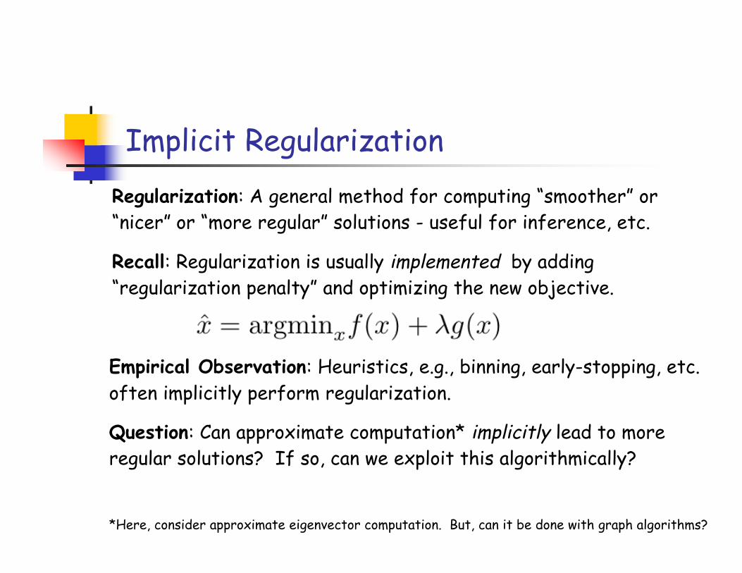
Implicit RegularizationRegularization: A general method for computing “smoother” or“nicer” or “more regular” solutions - useful for inference, etc.

Recall: Regularization is usually implemented by adding“regularization penalty” and optimizing the new objective.

Empirical Observation: Heuristics, e.g., binning, early-stopping, etc.often implicitly perform regularization.

Question: Can approximate computation* implicitly lead to moreregular solutions? If so, can we exploit this algorithmically?

*Here, consider approximate eigenvector computation. But, can it be done with graph algorithms?

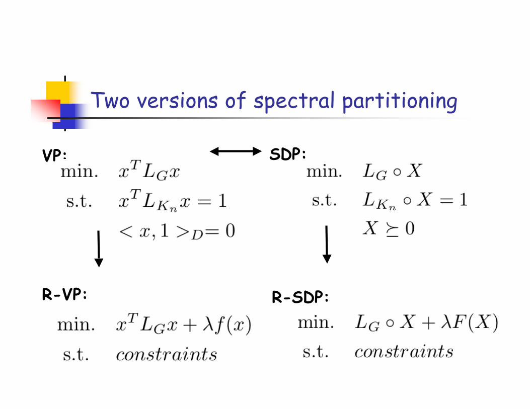
Two versions of spectral partitioning

VP: SDP:

R-SDP:R-VP:

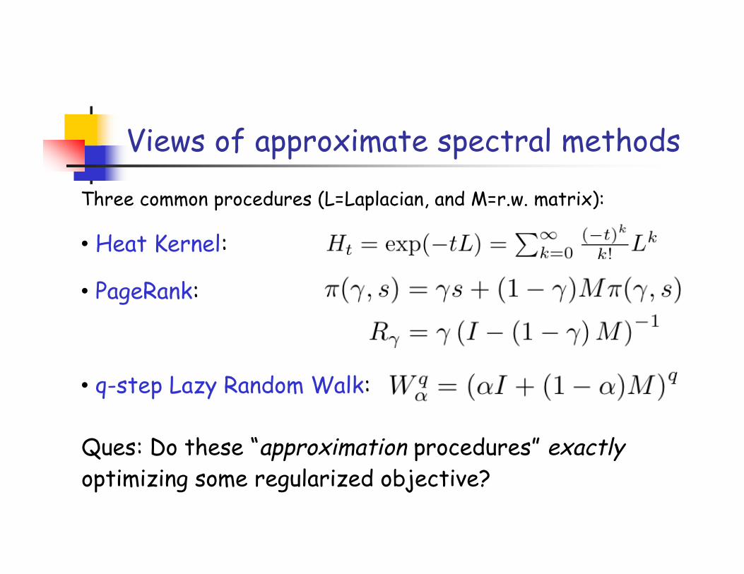
Views of approximate spectral methods

Three common procedures (L=Laplacian, and M=r.w. matrix):

• Heat Kernel:

• PageRank:

• q-step Lazy Random Walk:

Ques: Do these “approximation procedures” exactlyoptimizing some regularized objective?

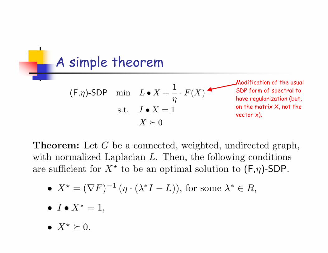
A simple theoremModification of the usualSDP form of spectral tohave regularization (but,on the matrix X, not thevector x).

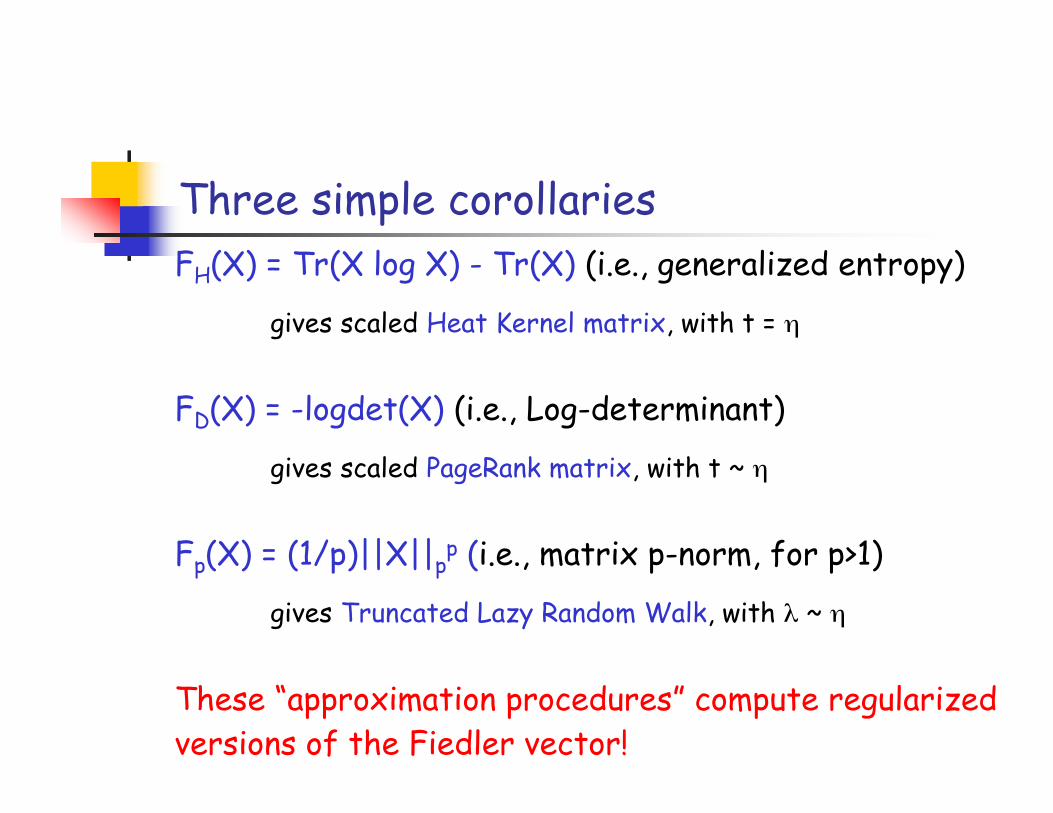
Three simple corollariesFH(X) = Tr(X log X) - Tr(X) (i.e., generalized entropy)

gives scaled Heat Kernel matrix, with t = η

FD(X) = -logdet(X) (i.e., Log-determinant)

gives scaled PageRank matrix, with t ~ η

Fp(X) = (1/p)||X||pp (i.e., matrix p-norm, for p>1)

gives Truncated Lazy Random Walk, with λ ~ η

These “approximation procedures” compute regularizedversions of the Fiedler vector!

Large-scale applications

A lot of work on large-scale data already implicitlyuses these ideas:

• Fuxman, Tsaparas, Achan, and Agrawal (2008): random walks onquery-click for automatic keyword generation

• Najork, Gallapudi, and Panigraphy (2009): carefully “whittlingdown” neighborhood graph makes SALSA faster and better

• Lu, Tsaparas, Ntoulas, and Polanyi (2010): test which page-rank-like implicit regularization models are most consistent with data

Question: Can we formalize this to understand when itsucceeds and when it fails?

Data Application 2: Classification in ML

Supervised binary classification• Observe (X,Y) ε (X,Y) = ( Rn , {-1,+1} ) sampled from unknown distribution P

• Construct classifier α:X->Y (drawn from some family Λ, e.g., hyper-planes) afterseeing k samples from unknown P

Question: How big must k be to get good prediction, i.e., low error?• Risk: R(α) = probability that α misclassifies a random data point

• Empirical Risk: Remp(α) = risk on observed data

Ways to bound | R(α) - Remp(α) | over all α ε Λ

• VC dimension: distribution-independent; typical method

• Annealed entropy: distribution-dependent; but can get much finer bounds

Unfortunately …Sample complexity of dstbn-free learning typically depends onthe ambient dimension to which the data to be classified belongs

• E.g., Ω(d) for learning half-spaces in Rd.

Very unsatisfactory for formally high-dimensional data

• approximately low-dimensional environments (e.g., close to manifolds,empirical signatures of low-dimensionality, etc.)

• high-variability environments (e.g., heavy-tailed data, sparse data, pre-asymptotic sampling regime, etc.)

Ques: Can distribution-dependent tools give improved learningbounds for data with more realistic sparsity and noise?

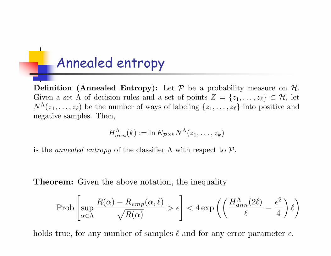
Annealed entropy

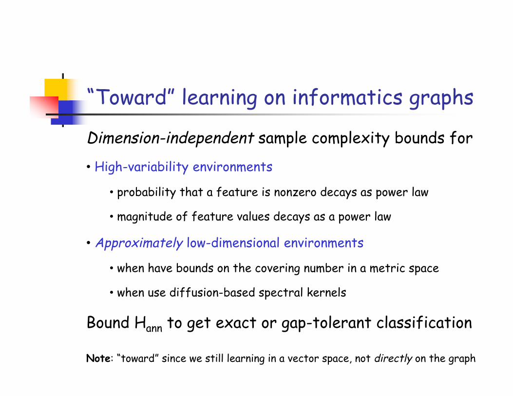
“Toward” learning on informatics graphs

Dimension-independent sample complexity bounds for

• High-variability environments

• probability that a feature is nonzero decays as power law

• magnitude of feature values decays as a power law

• Approximately low-dimensional environments

• when have bounds on the covering number in a metric space

• when use diffusion-based spectral kernels

Bound Hann to get exact or gap-tolerant classification

Note: “toward” since we still learning in a vector space, not directly on the graph

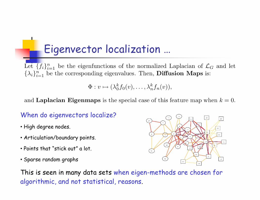
Eigenvector localization …

When do eigenvectors localize?• High degree nodes.

• Articulation/boundary points.

• Points that “stick out” a lot.

• Sparse random graphs

This is seen in many data sets when eigen-methods are chosen foralgorithmic, and not statistical, reasons.

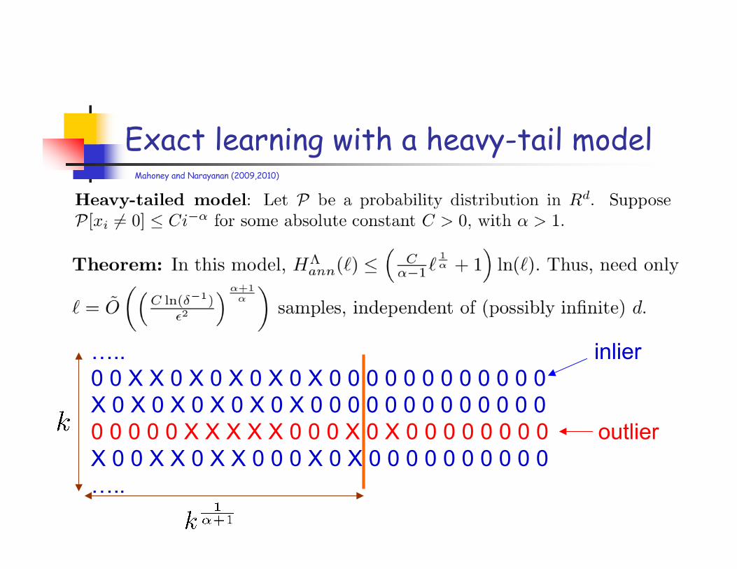
Exact learning with a heavy-tail model

….. inlier0 0 X X 0 X 0 X 0 X 0 X 0 0 0 0 0 0 0 0 0 0 0 0X 0 X 0 X 0 X 0 X 0 X 0 0 0 0 0 0 0 0 0 0 0 0 00 0 0 0 0 X X X X X 0 0 0 X 0 X 0 0 0 0 0 0 0 0 outlierX 0 0 X X 0 X X 0 0 0 X 0 X 0 0 0 0 0 0 0 0 0 0…..

Mahoney and Narayanan (2009,2010)

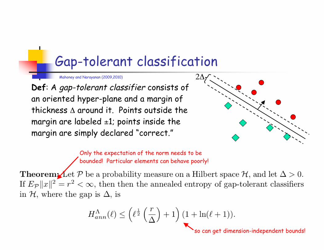
Gap-tolerant classification

Def: A gap-tolerant classifier consists ofan oriented hyper-plane and a margin ofthickness Δ around it. Points outside themargin are labeled ±1; points inside themargin are simply declared “correct.”

so can get dimension-independent bounds!

Only the expectation of the norm needs to bebounded! Particular elements can behave poorly!

Mahoney and Narayanan (2009,2010) 2Δ

Large-margin classification with very“outlying” data points

Apps to dimension-independent large-margin learning:• with spectral kernels, e.g. Diffusion Maps kernel underlying manifold-based methods, on arbitrary graphs

• with heavy-tailed data, e.g., when the magnitude of the elements of thefeature vector decay in a heavy-tailed manner

Technical notes:• new proof bounding VC-dim of gap-tolerant classifiers in Hilbert spacegeneralizes to Banach spaces - useful if dot products & kernels too limiting

• Ques: Can we control aggregate effect of “outliers” in other data models?

• Ques: Can we learn if measure never concentrates?

Mahoney and Narayanan (2009,2010)

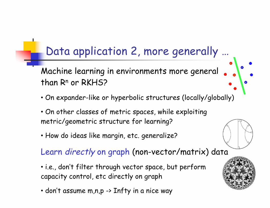
Data application 2, more generally …

Machine learning in environments more generalthan Rn or RKHS?

• On expander-like or hyperbolic structures (locally/globally)

• On other classes of metric spaces, while exploitingmetric/geometric structure for learning?

• How do ideas like margin, etc. generalize?

Learn directly on graph (non-vector/matrix) data

• i.e., don’t filter through vector space, but performcapacity control, etc directly on graph

• don’t assume m,n,p -> Infty in a nice way

Conclusions (1 of 4):General Observations

Network data are often very/extremely large:• Premium on fast/scalable algorithms• (Good - lots of algorithms; Bad - they often return meaningless answers.)

Network data are often very/extremely sparse:• Premium on statistical regularization• (Good - lots of regularization methods; Bad - they work on vectors, notgraphs.)• BTW, this implies “landmark point methods” often inappropriate

Networks have complex, nonlinear, adversarial structure• Structures don’t exist in small (e.g.,thousands of nodes) networks• Need tools to explore things we can’t visualize• Big difference between “analyst appls” and “next-user-interaction apps”

Conclusions (2 of 4):General Observations

• Algorithmic primitives to “probe” networks locally and globally

• Infer properties of original network from statistical andregularization properties of ensembles of approximate solutions

• Real informatics graphs -- very different than small commonly-studied graphs and existing generative models

• Tools promising for coupling local properties (often low-dimensional) and global properties (often expander-like)

• Tools promising to study pre-existing geometry versusgenerated geometry - recall geometry ≈ inference

• Validation is difficult - if you have a clean validation and/or apretty picture, you’re looking at unrealistic network data!

Conclusion (3 of 4) : “Structure” and“randomness” in large informatics graphs

High-level observations to formalize:• There do not exist a “small” number of linear components that capture“most” of the variance/information in the data.• There do not exist “nice” manifolds that describe the data well.• There is “locally linear” structure or geometry on small size scales thatdoes not propagate to global/large size scales.• At large size scales, the “true” geometry is more “hyperbolic” or “tree-like” or “expander-like”.

Important: even if you do not care about communities,conductance, hyperbolicity, etc., these empirical factsplace very severe constraints on the types of modelsand types of analysis tools that are appropriate.

Conclusion (4 of 4):Geometric Network Analysis Tools?

• Approximation algorithms have geometry hidden somewhereSpectral methods, LP methods, tree methods, metric embeddings

• Local Spectral MethodsIdentify geometry at multiple nodes at multiple size scalesNo need to assume local geometries are on a global manifold

• Approximate Computation as Implicit RegularizationApproximate solutions are better than exact solutionsEspecially relevant for extremely sparse/noisy networksUse this to regularize and do inference directly on network?

• Methodological test caseGood “hydrogen atom” for development of algorithmic andstatistical tools for probing graph data more generally