Embed Size (px)
Citation preview

i
SIMULATION OF AN INTEGRATED SOLAR ABSORPTION SYSTEM WITH
ORGANIC RANKINE CYCLE FOR SOIL COOLING APPLICATION
OLABOMI RASAQ ADEKUNLE
A thesis submitted in fulfilment of the
requirements for the award of the degree of
Doctor of Philosophy
Razak School of UTM in Engineering and Advanced Technology
Universiti Teknologi Malaysia
NOVEMBER 2017

ii
DECLARATION
I declare that this thesis entitled “Simulation of an Integrated Solar Absorption System
with Organic Rankine Cycle for Soil Cooling Application” is the result of my own
research except as cited in the references. The thesis has not been accepted for any
degree and is not concurrently submitted in candidature of any other degree.
Signature :
Name : OLABOMI RASAQ ADEKUNLE
Date : NOVEMBER, 2017

iii
DEDICATION
To my beloved (late) Parents; Alhaji Ahmad-Tijani Oladokun Olabomi and Hajia
Wulemat Aibinuola Olabomi,(نجن ميعن ت حيرن ن رن and my very wonderful family ,( ح

iv
ACKNOWLEDGEMENT
All thanks to Allah, who made it possible for me to complete this study at HIS
appointed time. Many thanks to Dr. Saad Abbas who accepted my proposal and introduced
me to Prof. Dato' Ir. Dr. A Bakar Jaafar, who then became my main supervisor, gave me
the supports to achieve my goal and the opportunity to work with him as a Research
Assistant under “eScience” Project. I thank my co-supervisors; Emeritus Prof. Dr. Md
Nor Musa, and Dr Shamsul Sarip for their unconditional support all through. I appreciate
the supports from management of Razak School, and from staff of Ocean Thermal Energy
Centre (Shaffiq Bin Rahmat, Azrin Bin Ariffin, and Ayuni Binti Romainodin).
I really appreciate the untiring support from my mentor, H.R.M Oba Abdul-
Rasheed Ayotunde Olabomi, and my entire family members. Iنcan’tنquantify the efforts
of my brothers and sisters; Alhaji T.A Olabomi, Sherifat Agboola, Dhikrullah Olawale
Olabomi, Muftau Kola Olabomi, Alhaja Jumoke Adeyemi, Alhaji Dele Alamu, Alhaji R.A
Lawal, and their wives and husbands. Special thanks to my friends; Yunus Adegboye,
Sunday Adeoye, Ademola Oladipo, Yakubu A. Momohjimoh, and others, who were
always on visit to my family at home during these periods. Dr. Umar, Dr Abubakar
Sulaiman, Dr Ali Gambo, Dr Obaji, Dr Yusuf Mohammed, and others can rarely be
thanked enough.
I thank the management of “Prototype Engineering Development Institute of
NASENI, Nigeria” for approving my study leave. Special thanks to the Muslim community
of the Institute, and to Mr. Hamzat H. Olaoye, whose personal efforts are unimaginable.
To my darling wife and children (Kafayat Omolola Olabomi, Faridah Omolade
Olabomi, and Sultan Adewole Olabomi), I really appreciate your patience, hopes, and
prayers at all times, without which this achievement might not be possible.
Ultimately, acknowledgement goes to Ministry of Science, Technology and
Innovation (MOSTI) Malaysia, for giving full financial support to this research under
eScience Fund (Project number: 06-01-06-SF1393)نforن“Integration of Rankine Power
and Absorption Refrigeration Cycles for Low Load Optimized Solar Thermal Chilled
Water Soil Cooling System”, from 1st of May 2015 to 31st of October 2017.
v
ABSTRACT
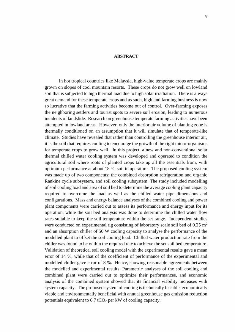
In hot tropical countries like Malaysia, high-value temperate crops are mainly
grown on slopes of cool mountain resorts. These crops do not grow well on lowland
soil that is subjected to high thermal load due to high solar irradiation. There is always
great demand for these temperate crops and as such, highland farming business is now
so lucrative that the farming activities become out of control. Over-farming exposes
the neighboring settlers and tourist spots to severe soil erosion, leading to numerous
incidents of landslide. Research on greenhouse temperate farming activities have been
attempted in lowland areas. However, only the interior air volume of planting zone is
thermally conditioned on an assumption that it will simulate that of temperate-like
climate. Studies have revealed that rather than controlling the greenhouse interior air,
it is the soil that requires cooling to encourage the growth of the right micro-organisms
for temperate crops to grow well. In this project, a new and non-conventional solar
thermal chilled water cooling system was developed and operated to condition the
agricultural soil where roots of planted crops take up all the essentials from, with
optimum performance at about 18 ºC soil temperature. The proposed cooling system
was made up of two components: the combined absorption refrigeration and organic
Rankine cycle subsystem, and soil cooling subsystem. The study included modelling
of soil cooling load and area of soil bed to determine the average cooling plant capacity
required to overcome the load as well as the chilled water pipe dimensions and
configurations. Mass and energy balance analyses of the combined cooling and power
plant components were carried out to assess its performance and energy input for its
operation, while the soil bed analysis was done to determine the chilled water flow
rates suitable to keep the soil temperature within the set range. Independent studies
were conducted on experimental rig consisting of laboratory scale soil bed of 0.25 m2
and an absorption chiller of 50 W cooling capacity to analyse the performance of the
modelled plant to offset the soil cooling load. Chilled water production rate from the
chiller was found to be within the required rate to achieve the set soil bed temperature.
Validation of theoretical soil cooling model with the experimental results gave a mean
error of 14 %, while that of the coefficient of performance of the experimental and
modelled chiller gave error of 8 %. Hence, showing reasonable agreements between
the modelled and experimental results. Parametric analyses of the soil cooling and
combined plant were carried out to optimize their performances, and economic
analysis of the combined system showed that its financial viability increases with
system capacity. The proposed system of cooling is technically feasible, economically
viable and environmentally beneficial with annual greenhouse gas emission reduction
potentials equivalent to 6.7 tCO2 per kW of cooling capacity.
vi
ABSTRAK
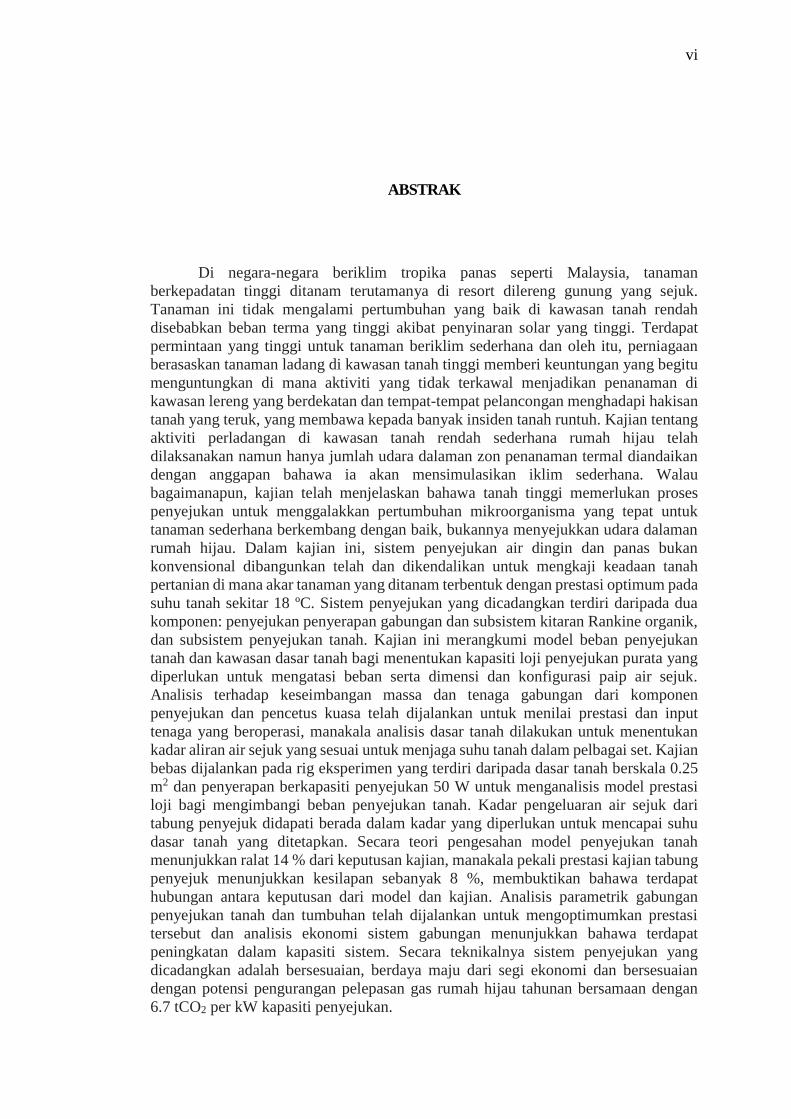
Di negara-negara beriklim tropika panas seperti Malaysia, tanaman
berkepadatan tinggi ditanam terutamanya di resort dilereng gunung yang sejuk.
Tanaman ini tidak mengalami pertumbuhan yang baik di kawasan tanah rendah
disebabkan beban terma yang tinggi akibat penyinaran solar yang tinggi. Terdapat
permintaan yang tinggi untuk tanaman beriklim sederhana dan oleh itu, perniagaan
berasaskan tanaman ladang di kawasan tanah tinggi memberi keuntungan yang begitu
menguntungkan di mana aktiviti yang tidak terkawal menjadikan penanaman di
kawasan lereng yang berdekatan dan tempat-tempat pelancongan menghadapi hakisan
tanah yang teruk, yang membawa kepada banyak insiden tanah runtuh. Kajian tentang
aktiviti perladangan di kawasan tanah rendah sederhana rumah hijau telah
dilaksanakan namun hanya jumlah udara dalaman zon penanaman termal diandaikan
dengan anggapan bahawa ia akan mensimulasikan iklim sederhana. Walau
bagaimanapun, kajian telah menjelaskan bahawa tanah tinggi memerlukan proses
penyejukan untuk menggalakkan pertumbuhan mikroorganisma yang tepat untuk
tanaman sederhana berkembang dengan baik, bukannya menyejukkan udara dalaman
rumah hijau. Dalam kajian ini, sistem penyejukan air dingin dan panas bukan
konvensional dibangunkan telah dan dikendalikan untuk mengkaji keadaan tanah
pertanian di mana akar tanaman yang ditanam terbentuk dengan prestasi optimum pada
suhu tanah sekitar 18 ºC. Sistem penyejukan yang dicadangkan terdiri daripada dua
komponen: penyejukan penyerapan gabungan dan subsistem kitaran Rankine organik,
dan subsistem penyejukan tanah. Kajian ini merangkumi model beban penyejukan
tanah dan kawasan dasar tanah bagi menentukan kapasiti loji penyejukan purata yang
diperlukan untuk mengatasi beban serta dimensi dan konfigurasi paip air sejuk.
Analisis terhadap keseimbangan massa dan tenaga gabungan dari komponen
penyejukan dan pencetus kuasa telah dijalankan untuk menilai prestasi dan input
tenaga yang beroperasi, manakala analisis dasar tanah dilakukan untuk menentukan
kadar aliran air sejuk yang sesuai untuk menjaga suhu tanah dalam pelbagai set. Kajian
bebas dijalankan pada rig eksperimen yang terdiri daripada dasar tanah berskala 0.25
m2 dan penyerapan berkapasiti penyejukan 50 W untuk menganalisis model prestasi
loji bagi mengimbangi beban penyejukan tanah. Kadar pengeluaran air sejuk dari
tabung penyejuk didapati berada dalam kadar yang diperlukan untuk mencapai suhu
dasar tanah yang ditetapkan. Secara teori pengesahan model penyejukan tanah
menunjukkan ralat 14 % dari keputusan kajian, manakala pekali prestasi kajian tabung
penyejuk menunjukkan kesilapan sebanyak 8 %, membuktikan bahawa terdapat
hubungan antara keputusan dari model dan kajian. Analisis parametrik gabungan
penyejukan tanah dan tumbuhan telah dijalankan untuk mengoptimumkan prestasi
tersebut dan analisis ekonomi sistem gabungan menunjukkan bahawa terdapat
peningkatan dalam kapasiti sistem. Secara teknikalnya sistem penyejukan yang
dicadangkan adalah bersesuaian, berdaya maju dari segi ekonomi dan bersesuaian
dengan potensi pengurangan pelepasan gas rumah hijau tahunan bersamaan dengan
6.7 tCO2 per kW kapasiti penyejukan.

vii
TABLE OF CONTENTS
CHAPTER TITLE PAGE
DECLARATION ii
DEDICATION iii
ACKNOWLEDGEMENT iv
ABSTRACT v
ABSTRAK vi
TABLE OF CONTENTS vii
LIST OF TABLES xii
LIST OF FIGURES xiv
LIST OF ABBREVIATIONS xvii
LIST OF SYMBOLS xviii
LIST OF APPENDICES xix
1 INTRODUCTION 1
1.1 Background 1
1.1.1 Energy Demand and Cooling Systems 3
1.1.2 Radiant Soil Cooling 4
1.1.3 Planted Crops and Soil Temperature 5
1.2 Problem Statement 6
1.3 Research Objectives 7
1.4 Scope of the Research 8
1.5 Significance of the Study 9
1.6 Research Questions 10
1.7 Thesis Organization 10
2 LITERATURE REVIEW 13
2.1 Introduction 13
2.2 Energy Issues and Renewable Energy Option 15

viii
2.3 Solar Energy Potentials in the Tropics 17
2.4 Solar Field 22
2.4.1 Solar Collectors 23
2.4.2 Performance Indicators 24
2.5 Solar Cooling Systems 26
2.5.1 Solar Absorption Cooling System 26
2.5.2 Absorption Chiller System 26
2.5.3 Basic Absorption Refrigeration Principles 28
2.5.4 Single, Double, and Multi-Effects Systems 29
2.5.5 Working Fluids and their Properties 30
2.6 Rankine Cycle and Organic Rankine Cycle 32
2.6.1 Organic Rankine Cycle (ORC) 33
2.6.2 Rankine Efficiency 35
2.6.3 Organic Working Fluids 36
2.7 ORC Integrations 36
2.8 Absorption Refrigeration–Organic Rankine Combined
Cycles 37
2.8.1 Combined Cooling, Heating and Power
System driven by Solar Energy 37
2.8.2 Rankine Cycle with Absorption Chiller 38
2.8.3 Goswami Cycle 39
2.8.4 Chilled Water Piping and Flow Rates 41
2.9 Radiant Cooling System 43
2.10 Agricultural Soil Cooling 45
2.10.1 Heat Transfer and Soil Thermal Properties 47
2.11 Economic Analysis 48
2.12 Summary 50
3 RESEARCH METHODOLOGY 52
3.1 Introduction 52
3.2 Cooling Load and Combined Plant Models 54
3.2.1 Soil Heat Transfer and Cooling Load Models 55
3.2.1.1 Soil Surface Heat Transfer 56
3.2.1.2 Soil Surface Heat Balance 57

ix
3.2.1.3 Soil Cooling Load 60
3.2.1.4 Vertical Heat Conduction 60
3.2.1.5 Chilled Water–Soil Heat Transfer 62
3.2.1.6 Earth Tube Material 65
3.2.2 Combined Plant Components Modelling and
Sizing 66
3.2.2.1 VAR–ORC Combined Plant
Components Modelling 69
3.2.3 Combined Plant–Cooling Load–Piping
Systems Integrations 74
3.2.4 Chilled Water Flow Rate Optimization 75
3.3 Energy Balance across the System Boundary 75
3.3.1 Steady State Energy Balance 75
3.3.2 Transient Energy Balance 77
3.4 Performance Evaluation 78
3.4.1 Power Cycle Efficiency 78
3.4.2 Cooling Coefficient of Performance 79
3.4.3 Combined Plant Performance 79
3.4.4 Soil Cooling Efficiency 80
3.5 Model Calculation with C# 81
3.5.1 Solution Algorithm Development 82
3.6 Experimental Investigation 82
3.6.1 Test Site Description 82
3.6.2 Experimental Set up 83
3.6.2.1 Soil Cooling Subsystem 84
3.6.2.2 Chilled Water Production
Subsystem 85
3.6.3 Data Collection Methods 87
3.6.4 Experimental Methods 90
3.6.5 Modified Cooling and Power System 91
3.7 Model Validation 94
3.8 Models Parametric Analysis 95
3.8.1 Soil Cooling Analysis 97
3.8.2 Combined Plant Analysis 98

x
3.8.2.1 Working Fluid Boiling Temperature 98
3.8.2.2 Turbine Inlet Pressure 99
3.8.2.3 Working Fluid Mass Fraction 99
3.9 Project Analysis with RETScreen® 99
3.9.1 Project Information and Site Reference
Conditions 100
3.9.2 Base Case Load and Network 101
3.9.3 Energy Model 101
3.9.4 Cost Analysis 101
3.9.5 Emission Analysis 102
3.9.6 Financial Analysis 103
3.10 Summary 104
4 RESULTS AND DISCUSSION 105
4.1 Introduction 105
4.2 Modelled Systems Characteristics 106
4.3 Analytical Results 106
4.3.1 Mass and Energy Balance across the System
Components 107
4.3.2 Cooling Production 109
4.3.3 Daytime Soil Cooling 109
4.4 Experimental Results 111
4.4.1 Cooling Production 111
4.4.2 Soil Temperature Profile 113
4.5 Models Comparison and Validation 115
4.5.1 Modelled and Experimental Soil Cooling
Rates 116
4.5.2 Modelled and Experimental Chilled Water
System 118
4.5.3 Component Analysis of the Experimental
Chiller 120
4.5.4 Combined Plant Analysis 121
4.6 Parametric Analysis of Soil Cooling System 122
4.7 Parametric Analysis of Combined Plant 125

xi
4.7.1 Gross Power (W_t) Sensitivity to Parameter
Variation 128
4.7.2 Pumping Power (W_sp) Sensitivity to
Parameter Variation 129
4.7.3 Heat Loss (Q_loss) Sensitivity to Parameter
Variation 130
4.7.4 Sensitivity on Cooling COP 131
4.7.5 ORC Efficiency Sensitivity to Parameter
Variation 132
4.7.6 Overall COP Sensitivity to Parameter
Variation 132
4.8 Plant Economic Analysis 134
4.9 Summary 136
5 CONCLUSIONS AND RECOMMENDATIONS 138
5.1 Conclusion 138
5.2 Recommendations 140
REFERENCES 142
Appendices A–I 161-191
xii
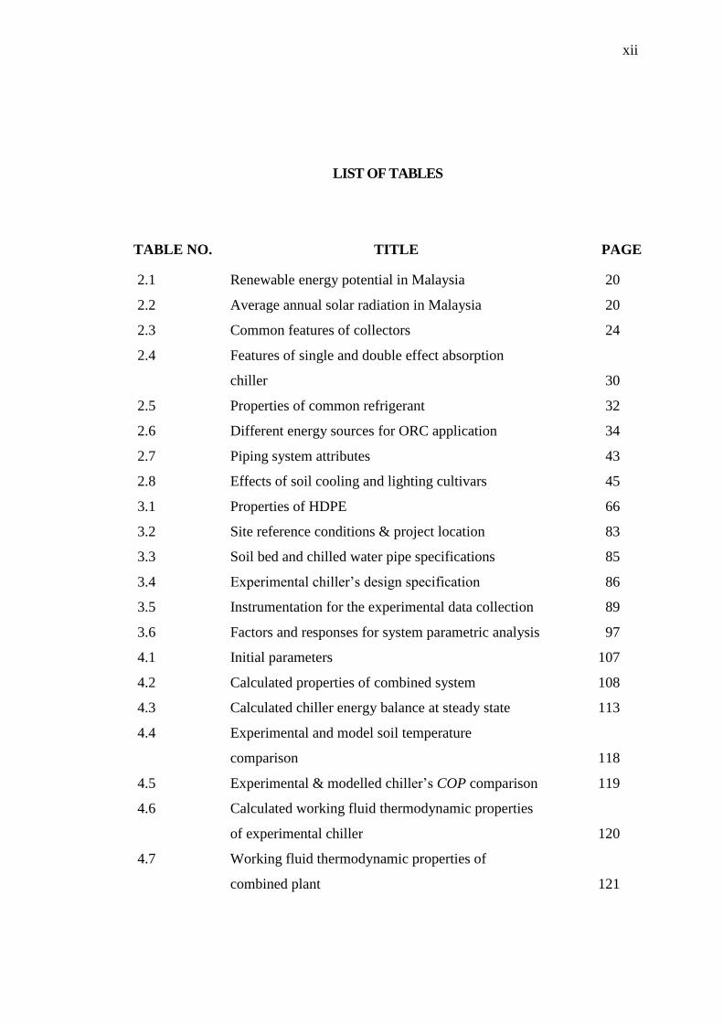
LIST OF TABLES
TABLE NO. TITLE PAGE
2.1 Renewable energy potential in Malaysia 20
2.2 Average annual solar radiation in Malaysia 20
2.3 Common features of collectors 24
2.4 Features of single and double effect absorption
chiller 30
2.5 Properties of common refrigerant 32
2.6 Different energy sources for ORC application 34
2.7 Piping system attributes 43
2.8 Effects of soil cooling and lighting cultivars 45
3.1 Properties of HDPE 66
3.2 Site reference conditions & project location 83
3.3 Soil bed and chilled water pipe specifications 85
3.4 Experimentalنchiller’sنdesignنspecification 86
3.5 Instrumentation for the experimental data collection 89
3.6 Factors and responses for system parametric analysis 97
4.1 Initial parameters 107
4.2 Calculated properties of combined system 108
4.3 Calculated chiller energy balance at steady state 113
4.4 Experimental and model soil temperature
comparison 118
4.5 Experimental & modelled chiller’sنCOP comparison 119
4.6 Calculated working fluid thermodynamic properties
of experimental chiller 120
4.7 Working fluid thermodynamic properties of
combined plant 121

xiii
4.8 Experimental chiller and combined plant energy
balance 122
4.9 Factors and response on soil cooling analysis 123
4.10 Factors and response on combined plant analysis 126
4.11 Factors-responses correlations for combined plant 127
4.12 Projects financial summary 135
4.13 Projects emission reduction summary 136

xiv
LIST OF FIGURES
FIGURE NO. TITLE PAGE
1.1 Effects of soil temperature on development of
planted crop 2
1.2 Conceptual solar VAR-ORC soil cooling system 7
2.1 Review process summary 14
2.2 Forms and classifications of energy 17
2.3 Daily solar radiations proportion on ground surface 18
2.4 Global latitudes of regions 19
2.5 Malaysia’sنpeakنdryنbulbنandنwetنbulbنtemperatures 21
2.6 Daytime horizontal solar radiation in Malaysia. 22
2.7 Basic single-effect absorption refrigeration cycle 29
2.8 Double-effect absorption refrigeration cycle 30
2.9 Schematic representation of Rankine cycle 33
2.10 Block representation of CCHP with ejector system 38
2.11 Rankine cycle with absorption chiller using WHR 39
2.12 Goswami combined power and refrigeration cycle 40
2.13 Constant primary flow configurations for chilled
water distribution 42
2.14 Deep seawater cold season vegetable bed 47
2.15 RETScreen® application paths 50
3.1 Methodology summary 53
3.2 Summarized chart for combined system modelling 54
3.3 Heat transfer model 55
3.4 Block representation of bare soil bed 57
3.5 Solar radiations on bare soil surface 58
3.6 Summarized flow for calculating pipe-soil heat
transfer 63

xv
3.7 Chilled water tube cross section and heat flows 63
3.8 Schematics of resistances to heat transfer across
chilled water tube 64
3.9 Integrated model of combined VAR–ORC system 67
3.10 Component energy balance model 70
3.11 ORC-VAR system boundary 76
3.12 System transient energy flow 77
3.13 Skematic representation of sub-model of absorption
chiller (A), and sub-model of soil bed cooling (B)
experimental set-up 84
3.14 Experimental soil bed and piping configuration 85
3.15 Experimental absorption refrigeration system 87
3.16 Components of the experimental (HN3/H2O) chiller
with chilled water storage 88
3.17 Schematic diagram of cooled experimental soil bed
with temperature and flowrate measurement 88
3.18 Validation path 95
3.19 RETScreen® application paths 100
4.1 Modelled soil temperatures profile during daytime at
different chilled water flowrates 110
4.2 Absorptionنchiller’sنoperatingنtemperatureنprofile 111
4.3 Calculated chilled water flow rate set at 5 ºC 113
4.4 Experimental soil temperature profiles at different
chilled water flow rates 114
4.5 Chilled water flow rate heat removal capacity 115
4.6 Experimental and modelled soil temperature profiles
for different chilled water flow rates 116
4.7 Average values of experimental and modelled soil
temperature profile 117
4.8 Model diagnostics plots for soil cooling analysis 124
4.9 3-D plots of chilled water and ambient air on cooled
soil 124
4.10 Effects of parameters variations on gross power
output 128

xvi
4.11 Effects of parameters variations on solution pump 129
4.12 Effects of parameters variations on heat loss 130
4.13 Effects of parameters variations on cooling COP 131
4.14 Effects of parameters variations on ORC efficiency 132
4.15 Effects of parameter variation on overall COP 133
4.16 Project annual cash flow 136

xvii
LIST OF ABBREVIATIONS
ANOVA - Analysis of Variance
B-C - Benefit-to-Cost
CCHP - Combined Cooling Heating and Power
COP - Coefficient of Performance
CPF - Constant Primary Flow
DOE - Design of Experiment
GHG - Greenhouse Gas
GSHP - Ground Source Heat Pump
HDPE - High Density Polyethylene
HHV - High Heating Value
HTF - Hot Thermal Fluid
HVAC - Heating Ventilation and Air Conditioning
IRR - Internal Rate of Return
LHV - Low Heating Value
NI - National Instrument
NIST - National Institute of Standard Technology
NPV - Net Present Value
OFAT - One Factor At a Time
ORC - Organic Rankine Cycle
RET - Renewable Energy Technology
RSM - Response Surface Methodology
VAR - Vapour Absorption Refrigeration
xviii
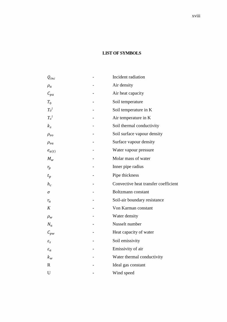
LIST OF SYMBOLS
𝑄𝑖𝑛𝑐 - Incident radiation
𝜌𝑎 - Air density
𝐶𝑝𝑎 - Air heat capacity
𝑇0 - Soil temperature
T01 - Soil temperature in K
Ta1 - Air temperature in K
𝑘𝑠 - Soil thermal conductivity
𝜌𝑣𝑜 - Soil surface vapour density
𝜌𝑣𝑎 - Surface vapour density
𝑒𝑎(𝑡) - Water vapour pressure
𝑀𝑤 - Molar mass of water
𝑟𝑝 - Inner pipe radius
𝑡𝑝 - Pipe thickness
ℎ𝑐 - Convective heat transfer coefficient
𝜎 - Boltzmann constant
𝑟𝑎 - Soil-air boundary resistance
K - Von Karman constant
𝜌𝑤 - Water density
𝑁𝑢 - Nusselt number
𝐶𝑝𝑤 - Heat capacity of water
𝜀𝑠 - Soil emissivity
𝜀𝑎 - Emissivity of air
𝑘𝑤 - Water thermal conductivity
R - Ideal gas constant
U - Wind speed

xix
LIST OF APPENDICES
APPENDIX TITLE PAGE
A Kuala Lumpur–Subang Station Meteorological and
Solar data 162
B Thermodynamic Properties of the Working Fluid at
Specified Conditions 164
C Solution Algorithm and Calculation
Implementation Codes in C# 167
D Experimental Set-up 170
E Soil Temperature Profile 171
F AbsorptionنChiller’sنPerformance 172
G Parametric Analysis of Soil Cooling and Combined
Plant 173
H Project Economic Analyses Details 182
I List of Publications 191

1
CHAPTER 1
1 INTRODUCTION
1.1 Background
Radiant cooling with chilled water is found suitable for a number of
applications (such as building comfort cooling, and agricultural soil cooling) in the
tropical climate countries. This is partly due to better thermal capacity of water, its
less pumping power requirement than the chilled air (Seo. et al., 2014), and most
importantly its effective removal of sensible heat either from living zone, or from the
agricultural soil. This is because human activity leading to heat generation is closer to
the floor than the ceiling, and microbial activities of planted crops mostly take place
in the soil. Meanwhile, high soil temperature affects the performance of crops
(Sattelmacher et al., 1990). Figure 1.1 shows the general effects of soil temperature
difference on root and shoot development of a planted crop. In addition, the operative
temperature of a room for instance, is greatly influenced by the radiant cooling as it
becomes the dominant process of heat transfer (Mikeska. and Svendsen, 2015). This
is therefore increasing the implementation of radiant soil (floor) cooling in the tropical
climate region as a way of reducing the air conditioning loads (Seo. et al., 2014).

2
Figure 1.1: Effects of soil temperature on development of planted crop (Yara, 2015)
Furthermore, implementation of soil cooling process towards the cultivation of
high-value temperate crops in the tropics is observed to be a more energy saving
process than air-cooled greenhouse systems, more importantly it has been established
that most of the physiological processes of planted crops are controlled by soil
temperature which if higher than optimal, will alter the root growth and functionalities
(Nabi and Mullins, 2008). However, soil temperature control requires energy
expenditure which if alternatively provided will make the system to be both
economically viable and environmentally benign. Applying solar thermal technology
to tackle solar radiation imposed load is one of the interesting research areas in the
tropics where there is high solar potential that is available in phase with the load.
Meanwhile, absorption cooling system and organic Rankine power cycle are typical
thermally activated technologies that are found suitable for utilization of low-grade
thermal energy such as geothermal and solar energy (Tchanche et al., 2011;
Khamooshi et al., 2013; Kim et al., 2012) through solar collector. Besides utilizing
low-grade thermal energy, the two cycles use organic working fluids, making their
combination for power and cooling an interesting research area in the recent time. This
study takes the advantage of the thermally activated technologies to overcome the
thermally imposed cooling load through the combined cooling and power plant cycle.
However, unlike previous studies on combined plant systems, cooling is the primary
goal in this study.
C C C C C C
3
1.1.1 Energy Demand and Cooling Systems
In the recent time, research on the application of renewable energy (such as
Solar, Wind, Geothermal, and Ocean thermal) is gaining more attention as a result of
the need to meet ever-growing energy demand (mostly for cooling), and environmental
issues. Solar thermal energy has been popular in the research field as a decentralized
renewable source of energy with higher application potentials in the tropical and sub-
tropical regions (Agyenim et al., 2010; Chua and Oh, 2012). Solar energy is a clean
and abundantly free source of energy which can be found anywhere on the surface of
the earth where day and night exist, and it is easily tapped at the point of use. A major
constraining factor for solar energy application is its seasonal nature resulting from its
availability that is directly tied to day and night cycle, and earth’s orbit around the sun
as well as the local weather condition of a place (such as rainfall, haze, typhoon and
cloud cover). Additionally, solar energy is generally a diffuse energy source (Hlbauer,
1986) and for it to be technologically useful, it must be captured using solar collector
which must be properly sized to avoid unnecessarily increased cost (Bajpai, 2012).
However, series of studies have been conducted on the use of thermal storage (Vadiee
and Martin, 2013; Nizami et al., 2013; Qu et al., 2010) as well as battery bank (Sanaye
and Sarrafi, 2015) to absorb the variation in solar energy supply.
Solar thermal energy has application potentials in diverse areas such as heating,
ventilation, and air-conditioning (HVAC) system as well as in electrical power
generating systems in domestic, industrial, commercial, and agricultural sectors. Solar
thermal applications for cooling systems have received increased research interest in
the recent time (Leavell, 2010; Lu et al., 2013; Agyenim et al., 2010; He et al., 2015),
likewise for Rankine systems to generate electrical power (Luzzi et al., 1999; Stodola
and Modi, 2009; Saitoh et al., 2007; Sanaye and Sarrafi, 2015). Regarded as low-
grade heat energy (Tchanche et al., 2011; Mikeska. and Svendsen, 2015), solar thermal
energy is found suitable for absorption cooling system and organic Rankine power
cycle because the two systems utilize working fluids that change phase at temperatures
below the boiling point of water and at low pressure (Arvay. et al., 2011). The
common features in the thermodynamic properties of the working fluids for the two
cycles have triggered more research interests in the combined power and cooling
4
system using organic Rankine cycle, and absorption refrigeration systems (Saitoh et
al., 2007; Datla, 2012; Abed et al., 2013; Ziviani et al., 2014; Padilla et al., 2010; Feng
et al., 2000; Tamm et al., 2004) and utilizing low-grade heat sources like solar,
geothermal, biomass and industrial waste heat.
1.1.2 Radiant Soil Cooling
For economic reasons and maintenance of sustainable environment, more
energy efficient measures are being analysed by researchers, mostly to meet the
cooling demands; during summer in the temperate regions, and year-round in the hot
and humid tropical regions. This has become imperative as the building energy
consumption accounts for about 40 % of the global energy consumption (Dong, 2010;
Khan et al., 2016). Heating ventilation and air-conditioning (HVAC) system accounts
for a larger percentage of this building energy consumption, amount of which depends
on the climatic region. In Oman, 54.7 % electricity in 2008 was consumed by building,
and air-conditioning took the larger percentage (Gastli and Charabi, 2011). More than
60 % of building electricity consumption the Kingdom of Saudi Arabia is taken by air-
conditioning and refrigeration systems (Said et al., 2012), most of which are vapour
compression types. About 33 % of the total Hong Kong electricity is consumed by
refrigeration and air conditioning system (Fong et al., 2010a). Furthermore, about 15
% of the global total electricity produced is consumed by refrigeration and air-
conditioning systems (Hong et al., 2011). However, radiant floor cooling methods
provide better indoor comfort in building with lower energy requirement relative to
conventional air cooling systems (Zarrella. et al., 2014; Zhao et al., 2016). The result
of the experimental field study on radiant cooling of a tropical residential building by
(Wongkee. et al., 2014a) shows 70 % energy saving compared to conventional air
conditioning system.
A major relative advantage of radiant cooling system over the traditional
HVAC system is its ability to be coupled with renewable energy sources, allowing
high efficiency and more energy savings thereby contributing to reduction in building

5
energy demand and total energy consumption (De Carli and Tonon, 2011; Wu. et al.,
2015; Yu. and Yao, 2015).
1.1.3 Planted Crops and Soil Temperature
The biochemical and physical activities taking place in the soil are effected by
soil temperature; influencing soil water movement and soil microbial activities (Nik.
et al., 1986), with the resultant effect on overall development of roots and shoots of
the planted crops (Nabi and Mullins, 2008). The effects of soil cooling and
supplemental lighting on five selected cultivars were investigated by (Labeke. and
Dambre, 1993) in which soil cooling contributed to increase in flower production of
the tested cultivars and extended the flowering production beyond winter to summer
periods.
Low soil temperature generally favours temperate crops. This is evident in the
cultivation of high-values temperate crops in some high altitudes in the tropics (such
as Cameron highland in Malaysia) where ambient air and soil temperatures are low.
As such, many research studies have been carried out on the cultivation of temperate
crops in the tropics (Mongkon et al., 2014; Mekhilef et al., 2013) but mostly based on
greenhouse farming systems.
Temperate crops can also thrive well on the tropical lowlands by cooling the
soil through hydronic/radiant cooling system. This is considered more energy efficient
than air cooling of the greenhouse currently in practice (Zhao. et al., 2014). With the
huge solar thermal potential in the tropics, the energy efficient soil cooling can be
achieved with innovative chilled water production from a combined plant of vapour
absorption refrigeration and organic Rankine power system, and its application for the
cooling process via network of buried pipes in a dimensioned soil bed.

6
1.2 Problem Statement
Tropical climate countries are mostly characterized with high ambient air
temperature and relative humidity. These have always constituted heavy cooling loads
and resultant increased energy demand for cooling in all sectors. Specifically, only
high temperature adaptive crops thrive well in the hot tropical region because, the year
round high air temperature and relative humidity are beyond the optimal level for most
high-value temperate crops making their cultivation in the tropics a serious challenge
due to heat stress (Peet et al., 2003; Max et al., 2009) that results from the heavy
cooling load. On the other hand, temperate regions are found to be generally cold with
temperature range between 10 ℃ and 20 ºC. Meanwhile, low soil temperature, with
average values between 14 ºC and 22 ºC favours the cultivation of most of the high-
value crops (Yara, 2015). High-value crops are non-staple agricultural crops (such as
fruits, vegetables, spices, condiments ornamentals and flowers,) that are known to have
higher return per hectare of land than other widely cultivated crops, presenting an
opportunity for farmers to increase their income (Othman et al., 2015). Some of these
crops are also cultivated in the tropics but with very low quality and at high cost of
cultivation except on some few highlands (hill/upland agriculture). Meanwhile this at
times results in erosion (Jim and Charles, 2009) and devastation of mountain
ecosystems and adjourning communities.
Besides highland farming, growing of temperate crops on lowlands in the
Tropics has mostly been through greenhouse farming system that involves air-
conditioning of entire volume of the planting zone with the intent to create temperate-
like thermal condition for the planted crops. However, most of the greenhouses
farming systems use conventional cooling that consumes huge amount of power,
thereby contributing to increase in energy demands. Sorption cooling systems could
be applied in this case but also require some amount of energy to operate the pumps
and other parasitic loads.
Thus, in this study, integration of vapour absorption refrigeration cycle with
organic Rankine cycle for simultaneous chilled water production and power
generation, using solar energy is proposed. The proposed system is based on the
7
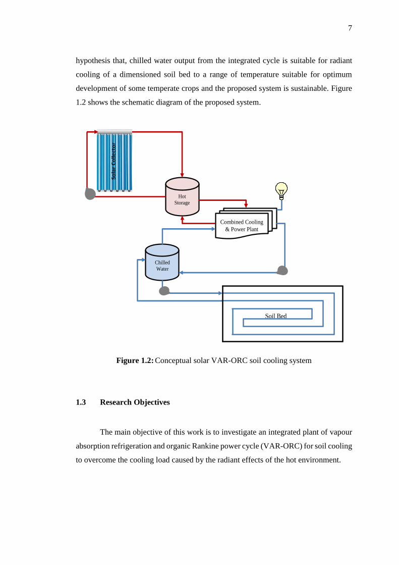
hypothesis that, chilled water output from the integrated cycle is suitable for radiant
cooling of a dimensioned soil bed to a range of temperature suitable for optimum
development of some temperate crops and the proposed system is sustainable. Figure
1.2 shows the schematic diagram of the proposed system.
Figure 1.2: Conceptual solar VAR-ORC soil cooling system
1.3 Research Objectives
The main objective of this work is to investigate an integrated plant of vapour
absorption refrigeration and organic Rankine power cycle (VAR-ORC) for soil cooling
to overcome the cooling load caused by the radiant effects of the hot environment.
Soil Bed
Chilled
Water
Tank
Hot
Storage
Tank
Combined Cooling
& Power Plant
So
lar
Co
lle
cto
r
8
The research objectives are:
i. To develop mathematical models of soil cooling load, and of the combined
plant cooling system performance.
ii. To develop a physical model to optimize the chilled water flow rate that
produces soil temperature distribution suitable for small scale temperate
crop farming.
iii. To develop test rig for the validation of the mathematical model.
iv. To analyse the economics of the developed system in comparison with that
of a conventional system of a similar cooling capacity.
1.4 Scope of the Research
Insulated box has been used for the experimental soil bed in this study and heat
transfer across the walls is assumed negligible. Similarly, since the experimental
chiller is small in capacity, requiring less than 0.5 m2 of solar collector to capture the
needed heat, activation of the chiller was achieved through an electric heater instead.
The study considered only the daytime application of chilled water for soil cooling,
and only the estimation of solar collector size required to capture the needed amount
of heat for running the system based on daily available solar radiation. Furthermore,
the soil used in this study is the local soil obtained from Kuala Lumpur. However,
with the idea of the soil characteristics, the developed model is suitable to estimate the
cooling load elsewhere. Other assumption to reduce the complexity of the model
equations include; (i) temperature profile in the pipe vicinity is not affected by the
presence of the pipe, as such, pipe surface temperature is uniform in the axial direction,
(ii) soil surrounding the pipe is homogeneous and has a constant thermal conductivity,
(iii) chilled water pipe has a uniform cross sectional area in the axial direction, (iv)
consideration is given to vertical heat conduction in the soil bed (Qin et al., 2002), (v)
undisturbed soil temperature is uniform around the chilled water pipe surface (Moncef
and Kreider, 1996) and equal to the external temperature of the pipe (Mongkon et al.,
2014), (vi) there exists a perfect contact between the earth tube (pipe) and the soil (Niu
9
et al., 2015), (vii) heat losses through the heat exchangers of the combined plant are
negligible (Rasih and Ani, 2012), (viii) pressure losses in piping and equipment are
considered negligibly small. The study is focused on cooling of agricultural soil to a
temperature range of 18 ºC ± 2, which is considered to be suitable for most high value
temperate crops.
1.5 Significance of the Study
The main focus of this research is to develop the concept of chilled water
production and power generation using low-grade solar energy, and application of the
chilled water for radiant soil cooling process. The expected result of the study is
significant but not limited to the following;
i. The result of this study intends to contribute to the better utilization of the
free energy source for simultaneous supply of power and cooling system.
ii. This study intends to serve as a tool for research focus on the application
of solar thermal chilled water for soil cooling as well as for comfort cooling
in agriculture and domestic building respectively. This is a less energy
consuming application.
iii. To also aid domestication of high-value temperate crops in the lowland
areas of the Tropics. This can be practiced on a small scale, and can
collectively contribute to the national economy by reducing the importation
of the so called temperate crops.
v. This combined plant is virtually a stand-alone system which can be applied
to radiant floor cooling system in domestic and public places with
advantages of reducing pressure on the energy demand and reducing the
environmental issues associated with the current cooling and primary
energy production systems.
10
1.6 Research Questions
Based on the objectives and scope of this study, the following questions are
intended to be answered;
i. With reference to the location and weather condition, what is the average
cooling load imposed on a meter-square of soil bed?
ii. What size of the soil bed (𝐴𝑠) can a certain plant capacity optimally cool,
and vice versa?
iii. What effective solar field area (𝐴𝑐) will optimally give the thermal energy
(𝑄𝑏) needed to vaporize the refrigerant to produce the desired cooling
(𝑄𝑒𝑣𝑝) and power (𝑊𝑡)?
iv. For a particular chilled water temperature, what is the optimized flow rate
to keep the soil temperature within the set range?
v. What is the overall performance of the combined plant and the soil cooling
system?
vi. Is the developed system economically impressive, and under what
conditions?
1.7 Thesis Organization
The thesis is majorly divided into five chapters; Chapter 1 (Introduction),
Chapter 2 (Literature Review), Chapter 3 (Methodology), Chapter 4 (Results and
Discussions), and Chapter 5 (Conclusions and Recommendations).
The introductory part of the thesis is focused on the background of the study as
it relates to the need for the cooling and the relative advantages of hydronic radiant
cooling against the traditional air cooling system as well as the application of
renewable energy for combined cooling and power systems. It also highlighted the
problems of the traditional systems of cooling and power and the available alternatives

11
to both cooling and power. Objectives of the study were set as well as the scope, and
significance of the study.
Chapter 2 is on the thorough review of the previous studies on both the
combined power and cooling systems, and the radiant cooling system but with focus
on agricultural soil cooling. It was discovered that these two areas of applications are
rarely combined: application chilled water from any source for radiant soil cooling,
and chilled water production from the combined plant have been individually reported
in the literature. However, in the reported combined plants, chilled water production
has always been a secondary goal to improve the efficiency of power generation.
Chapter 3 started with the modelling of the soil cooling load that is to be
overcome by the plant. This was done by taking the soil thermal properties and
location weather conditions into consideration. This was followed by modelling of the
chilled water piping network with reference to the pipe properties and expected
performance. Modelling of the combined plant capacity involves the components
sizing as well as performance optimization. For the implementation of the
mathematical models, software programming codes were developed for models
calculations. The experimental rig, consisting of ammonia based absorption chiller
and a dimensioned soil bed has been used to validate the modelled system. This was
followed by the parametric study of the soil cooling, and of the combined plant, using
RSM. The system economic analysis was carried out using RETScreen analysis
software.
Chapter 4 is on analysis of the analytical and experimental results, and
validation of the models. The results of the parametric analysis and optimization of
the combined plant are presented and discussed. The economic analyses, with the
financial viability and emission reduction resulting from implementing the developed
system, compared with a base case of similar capacity are also presented and discussed.

12
Chapter 5 is the conclusive summary of the thesis but with the emphasis on the
results and new discovery from the present study. Recommendations are also given on
the future areas of study.

13
CHAPTER 2
2 LITERATURE REVIEW
2.1 Introduction
This section of the study is focused on the issues surrounding the present
energy production and utilization, and applications of solar, as a free and safe energy
source for radiant soil cooling systems. The section covers the state of art review on;
i. Solar energy potentials, its harvesting and its contributions to the utilization
of HVAC in the tropical climate countries as well as its possible advantages
of reducing peak energy demand;
ii. The combined power and cooling cycles (utilizing low-grade thermal
energy) with focus on the combination of organic Rankine cycle and vapour
absorption refrigeration cycle (using NH3-H2O and other working fluids);
iii. Radiant soil cooling system, with more emphases on agricultural soil
cooling through the network of chilled water piping and pumping systems;
vii. Heat transfer and soil thermal properties as well as the influence of solar
radiation heat on the development of planted crops;
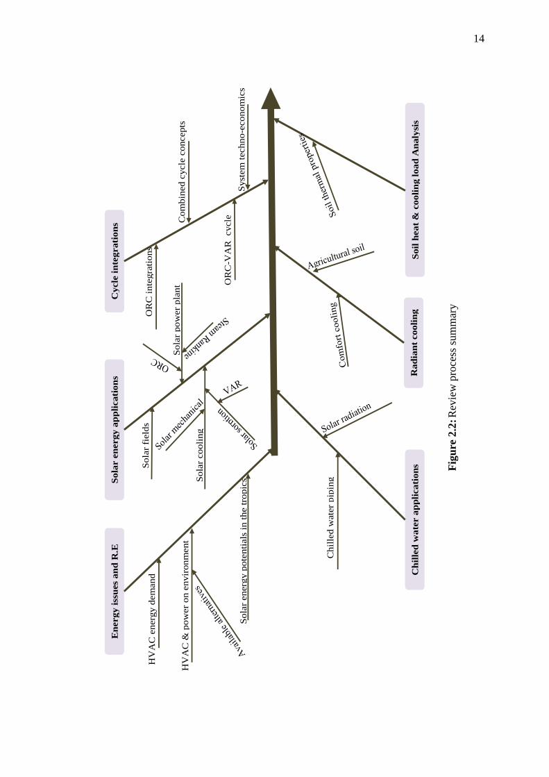
Review of various related theoretical and experimental studies on the subject
are presented so as to examine the outcome of this study with reference to other
published literatures. The summary of the review is presented in Figure 2.1.
14
Figure 2.1 Review process summary
E
nergy i
ssu
es
an
d R
.E
Sola
r e
nergy a
pp
licati
on
s C
ycle
in
tegrati
on
s
Sola
r cooli
ng
Sola
r pow
er
pla
nt O
RC
-VA
R cycle
HV
AC
& p
ow
er
on e
nvir
onm
ent
HV
AC
energ
y d
em
and
S
ola
r fi
eld
s
Sola
r energ
y p
ote
nti
als
in
the t
ropic
s
OR
C i
nte
gra
tions
Com
bin
ed c
ycle
concepts
Ch
ille
d w
ate
r a
pp
licati
on
s R
ad
ian
t cooli
ng
Soil
heat
& c
ooli
ng l
oad
An
aly
sis
Chil
led w
ate
r pip
ing
syst
em
s
Syst
em
techno
-econom
ics
Fig
ure
2.2
: R
evie
w p
roce
ss s
um
mar
y

15
2.2 Energy Issues and Renewable Energy Option
Energy is considered as the pivot of technology and modern day development
and as a result, it can be seen as the additional factor of production: after man, machine,
capital and entrepreneurship (Bajpai, 2012). At the same time the demand for energy,
particularly for cooling and heating is ever increasing (Deng et al., 2011). Conversely,
the larger proportion of the present global energy mix is non-renewable (Kaygusuz,
2012) and environmental unfriendly, necessitating the quest for alternative energy
sources. To achieve all-round development, it is paramount to secure a constant,
reliable, affordable and environmental friendly energy supply that must be efficiently
utilized for the required task, and in the long term, should constitute no threat to the
society.
Research interests have been focused on utilization of alternative and
renewable energy sources (such as solar, wind, biomass, geothermal, ocean thermal,
and tidal) due partly to the overwhelming awareness on issues of the current energy
supply, ranging from its imminent and fast depletion to environmental problems such
as ozone layer depletion, global warming and other pollutions resulting from their
production and/or application. Renewable energy sources are seen as green (Oh et al.,
2010), abundantly free (Marc et al., 2012), and with very little or no harmful effect on
environment either from their usage or their process of production (Chen, 2012).
To support the use of renewable energy, countries around the world have been
coming up with renewable energy policies that are targeted at mitigating the
environmental impacts occasioned by conventional energy sources and also to have
affordable and sustainable energy supplies, by providing motivation (in the form of
feed-in-tariff, subsidies and Renewable Portfolio Standard) towards the development
of renewable energy technologies (Solangi et al., 2011) and to be less reliant on fossil
fuel.
Malaysia ‘Renewable Energy Act (2011)’, is aimed at enhancing the utilization
of indigenous renewable energy sources for national electricity supply security and

16
sustainable socio-economic development through implementation of special tariff and
motivational incentives (Chen, 2012). This is expected to improve the renewable
energy proportion of the national power generation mix, enhance development of
renewable energy industries as well as conserving the environment (Solangi et al.,
2011). This implementation is with the involvement of a number of key Malaysian
government ministries and agencies in energy efficiency improvement (Mekhilef et
al., 2012). Pakistan Council of Renewable Energy Technology (PCRET) and
Alternative Energy Development Board (AEDB) were saddled with the responsibility
of implementation and actualization of renewable energy policy in Pakistan (Khan and
Pervaiz, 2013). Energy Performance Building Directive (EPBD) was established by
the European Parliament in 2002 and was modified in 2009 to mandate each of the
member states to set up minimum energy performance as well as to develop and
implement Energy Performance Certificate (EPC) for the building energy performance
rating (Boyano et al., 2013). In addition, in response to energy crisis witnessed in the
1973 between the Arab nations and the western world, Nigerian government
established the Energy Commission of Nigeria (ECN) in 1979 with the mandate to
conduct research and development (R&D) on renewable energy technologies and to
popularize its applications all over the country (Ilenikhena and Ezemonye, 2010). To
support the utilization of renewable energy, the Chinese National Development and
Reform Committee (NDRC) developed policies to support renewable electricity
generation, heating and cooling as well as RE research to replace oil in many
applications (Wang et al., 2009). Leading examples are found in Denmark, United
States of America, Canada, France, Spain, and Australia where favourable policies
were made to enhance renewable energy technologies (Mendonça et al., 2009; Solangi
et al., 2011).
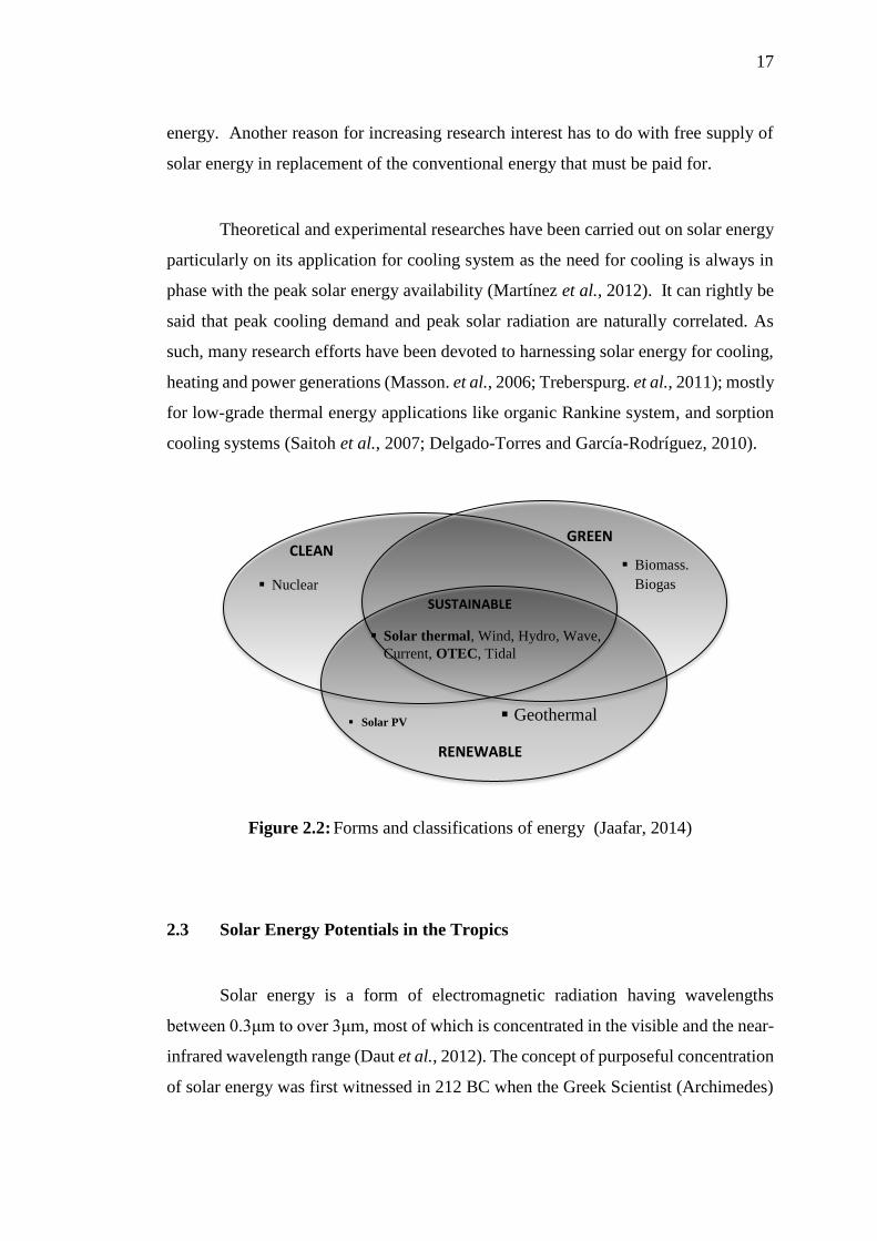
Of all the renewable energy sources, solar energy is found to be the most
promising source (as shown in Figure 2.2); it is in-exhaustive in supply and available
all over the world where day and night exist, and under no monopoly. It is estimated
that about 1.8 x 10¹¹MW of solar energy falls on the earth surface daily which if
properly utilized, could be more than the world energy consumption (Bajpai, 2012).
This is confirming the potential of solar energy as a promising source of alternative
17
energy. Another reason for increasing research interest has to do with free supply of
solar energy in replacement of the conventional energy that must be paid for.
Theoretical and experimental researches have been carried out on solar energy
particularly on its application for cooling system as the need for cooling is always in
phase with the peak solar energy availability (Martínez et al., 2012). It can rightly be
said that peak cooling demand and peak solar radiation are naturally correlated. As
such, many research efforts have been devoted to harnessing solar energy for cooling,
heating and power generations (Masson. et al., 2006; Treberspurg. et al., 2011); mostly
for low-grade thermal energy applications like organic Rankine system, and sorption
cooling systems (Saitoh et al., 2007; Delgado-Torres and García-Rodríguez, 2010).
Figure 2.2: Forms and classifications of energy (Jaafar, 2014)
2.3 Solar Energy Potentials in the Tropics
Solar energy is a form of electromagnetic radiation having wavelengths
between0.3نμmنtoنover3نμm, most of which is concentrated in the visible and the near-
infrared wavelength range (Daut et al., 2012). The concept of purposeful concentration
of solar energy was first witnessed in 212 BC when the Greek Scientist (Archimedes)
CLEAN
Nuclear
GREEN
Biomass.
Biogas
SUSTAINABLE
Solar thermal, Wind, Hydro, Wave,
Current, OTEC, Tidal
Geothermal Solar PV
RENEWABLE

18
devised a method to burn Roman war fleet using concave metallic mirrors (shinning
shield)نtoنconcentrateنtheنsun’sنraysنtoنburnنtheنRomanنfleetن(Kalogirou, 2004).
Solar thermal energy (Figure 2.3) has been very popular in the research field in
recent times as a decentralized energy source for power generation most importantly
in tropical and sub-tropical regions where the potential is relatively higher (Agyenim
et al., 2010; Chua and Oh, 2012). However, a major constraint is that it is a diffuse
energy source (Hlbauer, 1986), thus a solar collector is required to capture it in
technologically useful quantity: the collector must be properly sized to avoid
unnecessarily increased cost (Bajpai, 2012). Another constraining factor is the
seasonal nature of solar energy which results from its availability that is directly tied
to day and night cycle and earth’s orbit round the sun as well as the local weather
condition of a place such as haze, cloud cover, rainfall and typhoon (Mongkon et al.,
2013; Ssembatya. et al., 2014). However, this is usually taken care of by thermal
storage to bridge the demand gap (Ibrahim et al., 2017).
Figure 2.3: Daily solar radiations proportion on ground surface (NASA, 2017)
Generally, the Tropics is a region defined by the Tropic of Cancer in the
northern hemisphere with latitude of 23.5 ⁰N and the Tropic of Capricorn in the
southern hemisphere with latitude of 23.5 ⁰S (as shown in Figure 2.4). This region,
known as tropical zone is mostly found to be torrid. Most countries found in this region
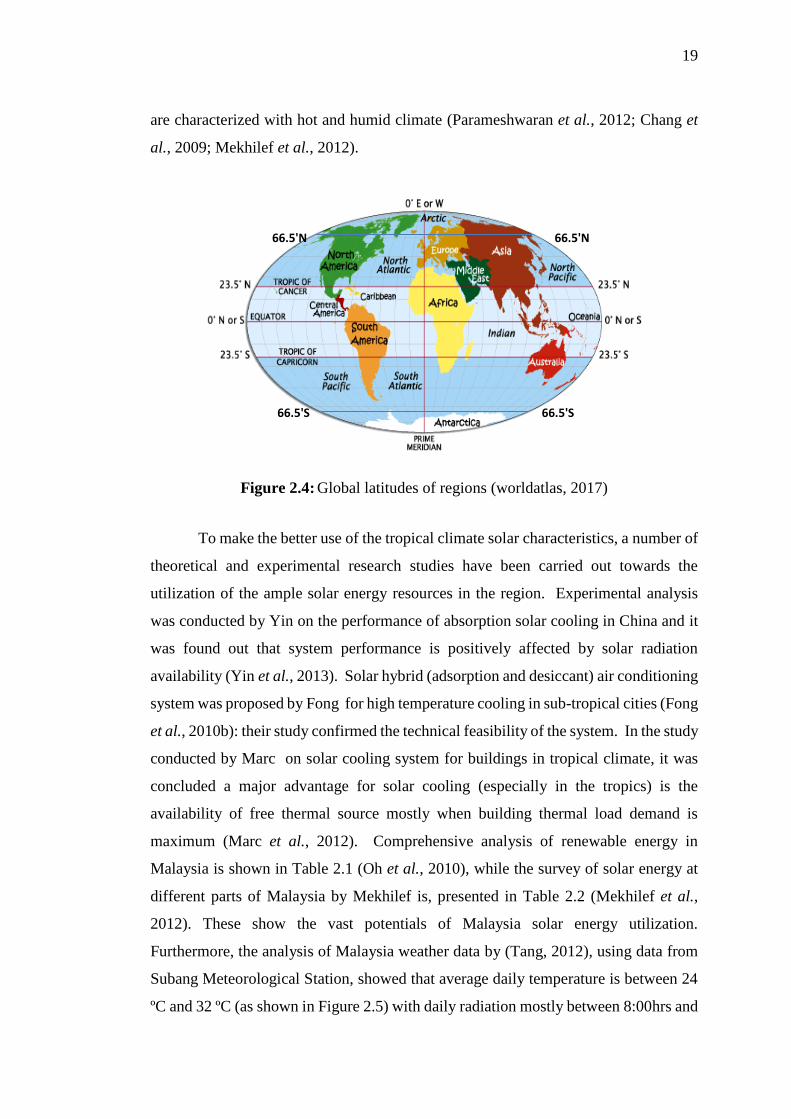
19
are characterized with hot and humid climate (Parameshwaran et al., 2012; Chang et
al., 2009; Mekhilef et al., 2012).
Figure 2.4: Global latitudes of regions (worldatlas, 2017)
To make the better use of the tropical climate solar characteristics, a number of
theoretical and experimental research studies have been carried out towards the
utilization of the ample solar energy resources in the region. Experimental analysis
was conducted by Yin on the performance of absorption solar cooling in China and it
was found out that system performance is positively affected by solar radiation
availability (Yin et al., 2013). Solar hybrid (adsorption and desiccant) air conditioning
system was proposed by Fong for high temperature cooling in sub-tropical cities (Fong
et al., 2010b): their study confirmed the technical feasibility of the system. In the study
conducted by Marc on solar cooling system for buildings in tropical climate, it was
concluded a major advantage for solar cooling (especially in the tropics) is the
availability of free thermal source mostly when building thermal load demand is
maximum (Marc et al., 2012). Comprehensive analysis of renewable energy in
Malaysia is shown in Table 2.1 (Oh et al., 2010), while the survey of solar energy at
different parts of Malaysia by Mekhilef is, presented in Table 2.2 (Mekhilef et al.,
2012). These show the vast potentials of Malaysia solar energy utilization.
Furthermore, the analysis of Malaysia weather data by (Tang, 2012), using data from
Subang Meteorological Station, showed that average daily temperature is between 24
ºC and 32 ºC (as shown in Figure 2.5) with daily radiation mostly between 8:00hrs and
66.5'N 66.5'N
66.5'S 66.5'S

20
18:00hrs clock time per day (as shown in Figure 2.6) but with usually high relative
humidity; between 66 % and 95 % (Tang, 2012).
Table 2.1: Renewable energy potential in Malaysia (Oh et al., 2010)
Renewable Energy Potential (MW)
Mini-hydro 500
Biomass/biogas (oil palm mill waste) 1,300
Municipal solid waste 400
Solar PV 6,500
Wind Low wind speed (less
than 2.0 m/sec)
Table 2.2: Average annual solar radiation in Malaysia (Mekhilef et al., 2012)
Irradiance Yearly average value (kWh/m2)
Kuching 1470
Bandar Baru Bangi 1487
Kuala Lumpur 1571
Petaling Jaya 1571
Seremban 1572
Kuantan 1601
Johor Bahru 1625
Senai 1629
Kota Baru 1705
Kuala Terengganu 1714
Ipoh 1739
Taiping 1768
George Town 1785
Bayan Lepas 1809
Kota Kinabalu 1900

21
Figure 2.5: Malaysia’s peak dry bulb and wet bulb temperatures (Tang, 2012)
Utilization of solar energy offers numerous advantages that include but not
limited to the following;
i. Aiding of decentralized energy supply and energy security;
ii. Environmental safety, as it involves no emission of greenhouse gases;
iii. Rural integration, especially in the developing countries of the world;
iv. Its application for water desalination helps in improving water quality and
quality of lives; and
v. Non-reliance on the gradually depleting fossil fuel.
Meanwhile some of the limitations/constraints include the high initial cost,
infancy of the technology (which can be addressed through continuous R&Ds), and
lack of proper awareness especially in the remote areas where it is most needed.
0
5
10
15
20
25
30
35
Tem
per
ature
(℃)
Time of the day (hr)
Peak dry bulb Temp Wet bulb Temp

22
Figure 2.6: Daytime horizontal solar radiation in Malaysia (Tang, 2012).
2.4 Solar Field
Solar energy is harvested through the solar photovoltaic (PV) cell, solar thermal
collector or their hybrid, referred to as PV/T (Khan and Pervaiz, 2013; Zhang et al.,
2012). Solar PV cells allow direct conversion of solar energy to electrical energy as
direct current (DC) or inverted to alternating current (AC) for appliance usage.
Meanwhile the obtainable efficiency from PV cells is usually between 9 % and 15 %
(Daut et al., 2012; Kalogirou, 2004; Gaglia et al., 2017), depending on the material
making up the PV cell. However, advances in solar PV technologies has actually
caused improvement from what it used to be in the last two decades (Kalogirou, 2004).
Solar thermal collectors do not directly convert solar energy to electrical energy
but it is used majorly to capture solar heat and supply it through thermal fluid for the
activation of HVAC systems (Duan et al., 2012; Tsoutsos. et al., 2009). The
coefficient of performance (COP) of solar collector is however between 0.7 and 2.0
(Fong et al., 2010b; Mokhtar et al., 2010), depending the type of the collector. Review
of solar thermal refrigeration systems was carried out by (Ullah et al., 2013) and it was
concluded thatن “theن solarن photovoltaicن systemن canن provideن electricityن asن wellن asن
refrigerationنbutنsolarنthermalنrefrigerationنisنmoreنefficient”.ننBasedنonنtheنscopeنofن
0
200
400
600
800
1000
1200
Rad
iati
on F
lux (
W/m
2)
Daytime (hr)
Min Rad. Max. Rad. Av. Rad.

23
this work, only solar thermal application is considered and solar energy is harvested
through the solar collector.
2.4.1 Solar Collectors
Basically solar collector constitutes an important part of solar thermal energy
utilization for heating (in form of domestic hot water and space heating), cooling (air-
conditioning/refrigeration), or for power generating system. Solar collector is a heat
exchanger containing absorber pipe with high absorptivity (~0.96) for short wave
length radiation and low emissivity (~0.04) for long wave radiation (Qu, 2008;
Kalogirou, 2004), making it able to absorb incoming solar radiation which is then
converted to heat energy of the transport fluid (such as air, water and oil) and
transferred through the fluid to the point of use. Solar collectors are broadly
categorized into concentrating and non-concentrating types which can be further sub-
divided to various types as shown in Table 2.3. Concentrating types are sun tracking
and consist of a wider parabolic shaped dish with reflecting mirrors that converge the
solarنradiationنtoنitsنvocalنpointنcalledن‘hotنspot’ن(Kadir and Rafeeu, 2010). Parabolic
dishes, parabolic through, and solar tower are major types of solar collector under
concentrating type and are more appropriate for industrial power cycles (Quoilin. and
Lemort, 2009; Price et al., 2002). Flat plate and evacuated tube are the most common
non-concentrating solar collectors (Chidambaram et al., 2011) and are most suitable
for low-grade temperature applications. These are also referred to as stationary
collectors. Non-concentrating collector is considered in this work.

24
Table 2.3: Common features of collectors (Mokhtar et al., 2010; Deng et al., 2011;
Bajpai, 2012)
Solar Collector Temp
Range (℃)
COP
(average) Application
Class Type
Non-
concentrating
Flat Plate 85 0.7 – 0.85 Single effect
Absorption
Evacuated
tube 85 0.7 – 0. 85 Single effect absorption
Concentrating
Parabolic
trough 180 1.4
Double effect
Absorption
Linear Fresnel 180 1.9 Triple effect
Absorption
Solar thermal
large scale
Parabolic
trough
250 2.0
Triple effect absorption
>350 Power block
Central
receiver
250 2.0
Triple effect absorption
>350 Power block
2.4.2 Performance Indicators
Most often, the performance indicators of interest in solar cooling systems are
the solar fraction (𝑆𝑓𝑟𝑎𝑐𝑡𝑖𝑜𝑛), solar thermal gain (𝐺𝑡ℎ𝑒𝑟𝑚𝑎𝑙), and coefficient of
performance (𝐶𝑂𝑃) (Fong et al., 2009).
Solar fraction (𝑆𝑓𝑟𝑎𝑐𝑡𝑖𝑜𝑛) is a measure of proportion of solar energy
contribution to the total energy required by solar cooling system to drive its
refrigeration unit. This is usually applicable when an auxiliary heat supply is involved
(Kadir and Rafeeu, 2010). Solar fraction of value close to 1 is an indication that the
system is more energy efficient. Thus the value of solar fraction will be zero if no
solar energy is involved and 1.0 if the system is totally driven by solar energy.
𝑆𝑓𝑟𝑎𝑐𝑡𝑖𝑜𝑛 =𝑄𝑠𝑜𝑙𝑎𝑟
𝑄𝑠𝑜𝑙𝑎𝑟+𝑄𝑎𝑢𝑥 (2.1)

25
Where 𝑄𝑠𝑜𝑙𝑎𝑟 and 𝑄𝑎𝑢𝑥 are the respective solar energy and auxiliary heat supplied to
activate the system.
Solar thermal gain (𝐺𝑡ℎ𝑒𝑟𝑚𝑎𝑙) is the amount of useful solar energy that can be
obtained through the collector. This is however tied to the type of collector and the
intensity of solar radiation available (Fong et al., 2010b). The useful energy gained is
theoretically given as;
𝑄𝑢 = 𝐴𝑐𝑄𝑖𝑛𝑐𝜂𝑐 (2.2)
Where 𝐴𝑐 is the effective area of the collector, 𝑄𝑖𝑛𝑐 is the solar radiation intensity and
𝜂𝑐 is the thermal efficiency of the collector array.
Thus, the theoretical efficiency of the collector is given as;
𝜂𝑐 =𝑄𝑢
𝑄𝑖𝑛𝑐×𝐴𝑐 (2.3)
𝑄𝑢 can also be expressed in terms of the energy transfer to the thermal fluid,
that is;
𝑄𝑢 = ḿ𝐶𝑝(𝑇ℎ − 𝑇𝑙) (2.4)
Where ḿ and 𝐶𝑝 are the respective mass flow rate and specific heat capacity of the
thermal fluid, and 𝑇ℎ & 𝑇𝑙 are outlet and inlet temperatures of the thermal fluid,
respectively.
Coefficient of performance (𝐶𝑂𝑃) is the performance indicator that measures
the amount of heat energy consumed by a refrigerating unit to net refrigeration effect
of the cooling system. It is otherwise defined as the quotient between the heat absorbed
by the evaporator (𝑄𝑒𝑣𝑝) and the heat gained by the working fluid from the generator
(𝑄𝑔𝑒𝑛). For a sorption refrigeration system, the COP is given as;

26
𝐶𝑂𝑃 = 𝑄𝑒𝑣𝑝
𝑄𝑔𝑒𝑛 (2.5)
Where 𝑄𝑒𝑣𝑝 the refrigeration is effect and 𝑄𝑔𝑒𝑛 is the heat supplied by the generator.
2.5 Solar Cooling Systems
Solar cooling majorly comprises of solar electric compression cooling, solar
mechanical compression cooling, solar desiccant cooling, solar absorption cooling and
solar adsorption cooling (Fong et al., 2009; Baniyounes et al., 2013). However, based
on the scope of this research, only solar absorption cooling system is discussed in
detail.
2.5.1 Solar Absorption Cooling System
Solar absorption cooling/refrigeration system involves pumping of binary
mixture as working fluid (refrigerant and absorber) through a solution heat exchanger,
to the generator for vaporization of the refrigerant. The refrigerant causes the cooling
effect (in the evaporator) after being subjected to a pressure differential through the
expansion valve. The cooled refrigerant is used for cooling process, or to cool another
(heat transport) fluid for further cooling processes. Most common refrigerant-
absorbent (working fluid) pairs are Ammonia-water NH3-H2O), and Lithium bromide-
water (LiBr-H2O). Absorption cooling can be single, double or multiple effects system
(Kalkan et al., 2012). This is discussed in more detail in the following sections.
2.5.2 Absorption Chiller System
Historically, the idea of absorption refrigeration started in the 1700s when it
wasنdiscoveredنthatن‘ice’نcouldنbeنproducedنbyنevaporating water within an evacuated
27
container in the presence of sulfuric acid (Ullah et al., 2013). Ferdinand Carré (A
French Engineer/Scientist) in 1859 designed the first machine that used ammonia-
water working fluid pair to produce ice that was used for food store (Srikhirin. et al.,
2001; Kalkan et al., 2012) and got the first US patent for his absorption unit in 1860
(Deng et al., 2011). The new system (with water-lithium bromide working fluid) was
later introduced in 1950 (Ullah et al., 2013) for commercial purposes.
Absorption refrigeration is considered a closed cycle system that can be driven
by low-grade heat sources like waste heat, geothermal heat, and solar energy to achieve
cooling or refrigeration. Solar absorption cooling system is gaining research attention
in recent times as a result of increase interest in the quests for alternative energy
especially for HVAC systems. Meanwhile, one of the challenges with absorption
cooling system is its relatively low coefficient of performance (between 0.5 and 1.5)
compared with the compression type with COP in excess of 3.0 (Somers et al., 2011;
Agyenim et al., 2010; Kalogirou. et al., 2001). This COP also depends on the working
fluid and the number of stage/effect of the system. As a result, there are many
theoretical and experimental studies on absorption refrigeration system that aimed at
achieving better performance of the system. Studies were conducted by (Abdulateef.
et al., 2007; Abdulateef. et al., 2008) on the comparison of solar driven absorption
refrigerator, based on some selected working fluids to improve the system
performance. In another study, (Khamooshi et al., 2013) did the review of
thermodynamic properties of Ionic liquids as working fluids to overcome some
common challenges associated with the common absorption refrigeration working
fluids like LiBr-H2O and NH3-H2O. Furthermore, the design analysis of solar powered
absorption cooling system was carried out by (Bajpai, 2012), for a definite system to
determine the system optimum parameter. For better improvement on the efficiency
of absorption refrigeration system, an experimental study was conducted by (Sözen et
al., 2012) on a diffusion absorption refrigeration system (DARS) and they came up
with a low energy/cost design for the system. Review of absorption refrigeration
technologies was carried out by (Srikhirin. et al., 2001), considering single, double and
multiple effects and various working fluids to improve absorber performance and to
increase the technological interest in the field of absorption refrigeration systems.
Some of the observed advantages of absorption refrigeration system include;
28
i. Highly economical as it involves low or no maintenance because it has no
moving part;
ii. High reliability and long service life;
iii. Quiet (silent) operation and does not contribute to environmental
pollution;
vi. Helps in efficient energy utilization and more useful in remote places where
grid-tied electricity is a problem;
2.5.3 Basic Absorption Refrigeration Principles
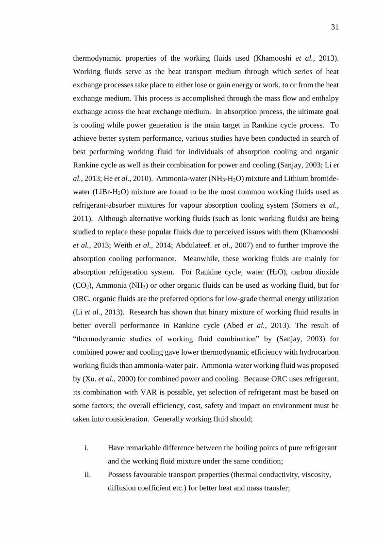
The basic absorption refrigeration cycle is presented in Figure 2.7 with the
main components as; absorber, generator, condenser, and evaporator (Khamooshi et
al., 2013). Starting from the absorber, low pressure aqua-ammonia solution
(containing refrigerant and absorbent) is pumped to the generator at elevated pressure.
The solution passes through a heat exchanger where it is preheated by the return stream
from the generator. Heat is supplied to the generator from the heat source which can
be solar collector, biomass, gas or electric heater, to drives off the refrigerant (in vapour
form) from the mixture of the weak solution. This is also referred to as desorption
(Somers et al., 2011; Kasperski and Eichler, 2012; Garimella, 2012). The liquid
absorbent returns to the absorber through the expansion valve that reduces its pressure.
The refrigerant (strong solution) vapour leaving the generator enters the condenser and
condenses into liquid, where it loses most of its heat (Cloutier, 2002). It then flows
through an expansion valve that causes reduction in its pressure. This pressure
reduction also causes reduction in saturation temperature of the refrigerant; making it
extremely cold (Gupta, 2011; Cai et al., 2014) saturated liquid which then evaporates
and extracts heat from the evaporator space before flowing into absorber tank where it
is absorbed to become weak, low-pressure saturated liquid to repeat the cycle again.
The heat extraction from the evaporator is referred to as refrigeration/cooling effect of
the system

29
Figure 2.7: Basic single-effect absorption refrigeration cycle
2.5.4 Single, Double, and Multi-Effects Systems
Absorption refrigeration system is also grouped (base on the number of
refrigerant vapour generation) into single-effect, double-effect, triple-effect or
multiple-effect (Deng et al., 2011; Garimella, 2012; Hong et al., 2011; Sharizal, 2006)
as shown in Table 2.4. The single effect type (Figure 2.7) operates at lower
temperature than double/triple/multi-effects types. Double-effect types (Figure 2.8), is
characterized with two generators and two solution heat exchangers (Sharizal, 2006).
Low pressure binary solution is pumped through HX1 to HX2 then to the generators 1
and 2 from where it flows to the condenser in which it is condensed and cooled before
flowing through the expansion valve to the evaporator and back to the absorption tank
to repeat the cycle. HX2 can also pass the solution to generator 2 which can as well
pass it to HX1. Literatures showed that two single-effects cycles can form a double-
effect cycle as the COP of double effect is relatively equal to two of the single-effects
COP (Srikhirin. et al., 2001; Ullah et al., 2013). The coefficient of performance of an
absorption refrigeration system is expressed as;
𝐶𝑂𝑃 =𝐶𝑜𝑜𝑙𝑖𝑛𝑔 𝑐𝑎𝑝𝑎𝑐𝑖𝑡𝑦 𝑎𝑐ℎ𝑖𝑒𝑣𝑒𝑑
𝐺𝑒𝑛𝑒𝑟𝑎𝑡𝑜𝑟 ℎ𝑒𝑎𝑡 𝑖𝑛𝑝𝑢𝑡+𝑤𝑜𝑟𝑘 𝑑𝑜𝑛𝑒 𝑜𝑛 𝑡ℎ𝑒 𝑝𝑢𝑚𝑝 (2.6)
Evaporator
Condenser
Heat exchanger
Absorber
Generator

30
Figure 2.8: Double-effect absorption refrigeration cycle (Ullah et al., 2013; Srikhirin.
et al., 2001)
Table 2.4: Features of single and double effect absorption chiller (Deng et al., 2011;
Srikhirin. et al., 2001)
Properties Single-effect Double-effect
Working
fluids LiBr-H2O NH3-H2O LiBr-H2O NH3-H2O
Operating
pressure and
temperature
2 – 3 bar, 70 –
100 ℃ hot
water or direct
fired
2 – 16 bar,
steam or 70 –
110 ℃ hot
water
4 – 8 bar,
steam or 120 –
170 ℃ hot
water
8 – 16 bar, steam
or 170 – 220 ℃
hot water
Refrig. output 5 – 10 ℃ chilled water 5 – 10 ℃ chilled water
Capacity
range 5 – 7,000 kW 4.5 – 90 kW
20 – 11,630
kW <110kW
Cooling
method
Water-cooled or air-cooled
(small unit) Water-cooled or air-cooled
COP range 0.5 – 0.7 0.5 – 0.75 0.7 – 1.2 0.7 – 1.2
2.5.5 Working Fluids and their Properties
Working fluid is vital to both the absorption cooling system and organic
Rankine system, because the performance of both cycles depends on the
HX2
Evaporator
Generator 2
Absorber
Generator 1
HX1
Condenser
31
thermodynamic properties of the working fluids used (Khamooshi et al., 2013).
Working fluids serve as the heat transport medium through which series of heat
exchange processes take place to either lose or gain energy or work, to or from the heat
exchange medium. This process is accomplished through the mass flow and enthalpy
exchange across the heat exchange medium. In absorption process, the ultimate goal
is cooling while power generation is the main target in Rankine cycle process. To
achieve better system performance, various studies have been conducted in search of
best performing working fluid for individuals of absorption cooling and organic
Rankine cycle as well as their combination for power and cooling (Sanjay, 2003; Li et
al., 2013; He et al., 2010). Ammonia-water (NH3-H2O) mixture and Lithium bromide-
water (LiBr-H2O) mixture are found to be the most common working fluids used as
refrigerant-absorber mixtures for vapour absorption cooling system (Somers et al.,
2011). Although alternative working fluids (such as Ionic working fluids) are being
studied to replace these popular fluids due to perceived issues with them (Khamooshi
et al., 2013; Weith et al., 2014; Abdulateef. et al., 2007) and to further improve the
absorption cooling performance. Meanwhile, these working fluids are mainly for
absorption refrigeration system. For Rankine cycle, water (H2O), carbon dioxide
(CO2), Ammonia (NH3) or other organic fluids can be used as working fluid, but for
ORC, organic fluids are the preferred options for low-grade thermal energy utilization
(Li et al., 2013). Research has shown that binary mixture of working fluid results in
better overall performance in Rankine cycle (Abed et al., 2013). The result of
“thermodynamicن studiesن ofن workingن fluidن combination”ن byن (Sanjay, 2003) for
combined power and cooling gave lower thermodynamic efficiency with hydrocarbon
working fluids than ammonia-water pair. Ammonia-water working fluid was proposed
by (Xu. et al., 2000) for combined power and cooling. Because ORC uses refrigerant,
its combination with VAR is possible, yet selection of refrigerant must be based on
some factors; the overall efficiency, cost, safety and impact on environment must be
taken into consideration. Generally working fluid should;
i. Have remarkable difference between the boiling points of pure refrigerant
and the working fluid mixture under the same condition;
ii. Possess favourable transport properties (thermal conductivity, viscosity,
diffusion coefficient etc.) for better heat and mass transfer;

32
iii. Be thermally stable, non-flammable, non-corrosive, non-toxic and non-
fouling;
iv. Be regularly available at reasonable cost;
v. Have low operating temperature and pressure;
In reality, all the desirable properties may be difficult to achieve from a
particular working fluid for a particular purpose. Some of the refrigerants with their
properties are shown in Table 2.5.
Table 2.5: Properties of common refrigerant (Khennich and Galanis, 2012; Kim et
al., 2012; NIST; McQuay, 2002)
Refrigerant Common Application 𝑻 𝒄𝒓𝒊𝒕
(℃)
𝑻 𝒃𝒐𝒊𝒍
(℃)
𝑷 𝒄𝒓𝒊𝒕
(Bar) ODP GWP
R-114 (C2F4Cl2) Sorption cooling 145.7 32.5 14.8 1 3.9
R-245fa (C3H3F5) ORC 154 14.4 36.34 0 820
R-290 Propane
(CH3CH2CH3) ORC 96.7 -42.1 42.5 0 0
R-124 (C2HF4Cl) Sorption cooling 122.5 -12.1 36.4 0.02 620
R-125
(CHF2CF3) Sorption cooling 66.1 -54.6 36.3 0 2800
R-134a
(CH2FCF3)
Sorption cooling, ORC
Power 101.1 -26.1 4.6 0 1300
R-143a (C2H3F3) Sorption cooling 73.1 38.1 0 4300
R-152a (C2H4F2) Sorption cooling 113.6 -24.0 44.9 0 120
R-32 (CH2F2) Sorption cooling 7
8.1 -51.7 57.8 0 650
R-718 (H2O) Sorption cooling, RC 373.9 100 220.6 0 < 1
R-717 (NH3) Sorption, ORC 132.2 -33.3 42.5 0 0
2.6 Rankine Cycle and Organic Rankine Cycle
Traditional steam Rankine cycle has been applied in the past to generate power
but with very high operating temperature and pressure (Kalogirou, 2004). The power

33
range is usually quite large and generally in the range of 10MWe and above with
relatively low efficiency; around 10 % (Arvay. et al., 2011). Basically, Rankine cycle
(Figure 2.9) involves four main steps (Sanjay, 2003; Arvay. et al., 2011), which are;
i. Pumping of working fluid from low pressure to the boiler, at high
pressure;
ii. Heating/superheating of the working fluid at constant pressure in the
boiler to vaporise the working fluid;
iii. Expansion of the vaporized working fluid through the turbine from which
the mechanical work is converted to electrical energy;
iv. Condensation of the working fluid through the condenser before it is
pumped back to repeat the cycle;
Figure 2.9: Schematic representation of Rankine cycle
2.6.1 Organic Rankine Cycle (ORC)
The growing interest in the application of low-to-moderate grade heat energy
has made organic Rankine cycle (ORC) popular in the recent times (Ziviani et al.,
2014). Organic Rankine cycle is similar in configuration and principle to the
traditional steam Rankine cycle (Leslie. et al., 2009) except that;
i. It uses organic working fluid with favourable thermodynamic properties.
Boiler
Condenser
Tu
rbin
e
Pump
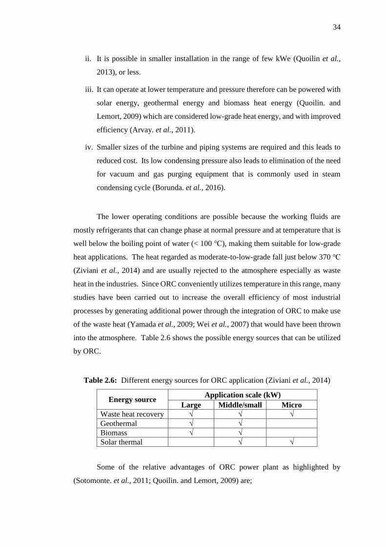
34
ii. It is possible in smaller installation in the range of few kWe (Quoilin et al.,
2013), or less.
iii. It can operate at lower temperature and pressure therefore can be powered with
solar energy, geothermal energy and biomass heat energy (Quoilin. and
Lemort, 2009) which are considered low-grade heat energy, and with improved
efficiency (Arvay. et al., 2011).
iv. Smaller sizes of the turbine and piping systems are required and this leads to
reduced cost. Its low condensing pressure also leads to elimination of the need
for vacuum and gas purging equipment that is commonly used in steam
condensing cycle (Borunda. et al., 2016).
The lower operating conditions are possible because the working fluids are
mostly refrigerants that can change phase at normal pressure and at temperature that is
well below the boiling point of water (< 100 ℃), making them suitable for low-grade
heat applications. The heat regarded as moderate-to-low-grade fall just below 370 ℃
(Ziviani et al., 2014) and are usually rejected to the atmosphere especially as waste
heat in the industries. Since ORC conveniently utilizes temperature in this range, many
studies have been carried out to increase the overall efficiency of most industrial
processes by generating additional power through the integration of ORC to make use
of the waste heat (Yamada et al., 2009; Wei et al., 2007) that would have been thrown
into the atmosphere. Table 2.6 shows the possible energy sources that can be utilized
by ORC.
Table 2.6: Different energy sources for ORC application (Ziviani et al., 2014)
Energy source Application scale (kW)
Large Middle/small Micro
Waste heat recovery √ √ √
Geothermal √ √
Biomass √ √
Solar thermal √ √
Some of the relative advantages of ORC power plant as highlighted by
(Sotomonte. et al., 2011; Quoilin. and Lemort, 2009) are;

35
i. Higher cycle and turbine efficiencies;
ii. Low mechanical stress as a result of low tangential velocity;
iii. With organic liquid, risk of turbine blade erosion (due to moisture in the
vapour flow) is reduced;
iv. Equipment longer life span;
v. Requires no water treatment;
2.6.2 Rankine Efficiency
Generally, for thermal power plant, cycle efficiency is defined as the ratio of
power output to the heat input into the system; this efficiency is defined in terms of the
gross or net power output.
𝜂𝑔𝑟𝑜𝑠𝑠 =𝑃𝑔𝑟𝑜𝑠𝑠
Ǭ𝑏 (2.7)
𝜂𝑛𝑒𝑡 =𝑃𝑛𝑒𝑡
𝑄𝑏
𝑃𝑛𝑒𝑡 = 𝑃𝑔𝑟𝑜𝑠𝑠 − ∑ 𝑊𝑝𝑖 (2.8)
Where 𝑃𝑔 and 𝑃𝑛𝑒𝑡 are turbine gross and net power outputs, respectively, 𝑊𝑝𝑖 is the
power consumed to pump the working fluid, Ǭ𝑏 is boiler heat input to vaporize the
working fluid.
Working fluid plays an important role in the cycle efficiency of Rankine power
system, therefore one of the main challenges in ORC power system is the choice of
appropriate working fluid that can both give maximum efficiency (Karellas. and
Schuster, 2008) and be environmental friendly. The mathematical model by
(Sotomonte. et al., 2011) to find better organic working fluid for ORC in biomass
cogeneration reveals that the cycle efficiency depends more on the thermodynamic
properties of the working fluid than the system configuration.

36
2.6.3 Organic Working Fluids
Primary working fluid conveys the thermal energy from the solar collector to
the boiler where this thermal laden fluid is used to vaporize the organic fluid, which in
turn flows with high pressure to the turbine to perform useful work. Various organic
working fluids have been proposed and used for ORC. R113 (C2Cl3F3) was used by
(Saitoh et al., 2007) in the development and testing of solar organic Rankine cycle,
using scroll expander in the turbine. They then suggested the use of solar organic
Rankine system for future power generation and distribution on small scale. Pentane
was used by (Leslie. et al., 2009) as working fluid in ORC for capturing of 5.5MW of
electricity from 27MW output gas fired steam turbine. The additional energy was
achieved with no fuel addition and almost no emission. The result of mathematical
analysis by (Sotomonte. et al., 2011) confirmed that the efficiency of ORC is a function
of the thermodynamic properties of the organic working fluid. Studies by (Delgado-
Torres and García-Rodríguez, 2010) considered various working fluids (Propane,
R134a, R227ea, R152a, NH3, Isobutane, Butane, R245fa, Neopentane, R245ca,
Isopentane and Pentane) while working on the low-temperature (solar) application for
ORC. The consideration was based on their thermodynamic properties and effects on
the environment.
2.7 ORC Integrations
The possibility of integrating ORC with other cycles and its ability to utilize
heat energy from various low-grade heat sources had made it to become more popular
in recent times. Studies were conducted on optimization of ORC using low-grade heat
recovery (Ziviani et al., 2014), to evaluate the system ability to deliver the electricity,
heating and cooling (using electric air-conditioner) demands of a living apartment.
Combination of ORC with desalination technology was analysed (Delgado-Torres and
García-Rodríguez, 2010); their system was powered by solar energy through the solar
collector to produce fresh water in some areas with problem of rising water scarcity.
Ocean thermal energy conversion (OTEC) is an alternative energy extraction process
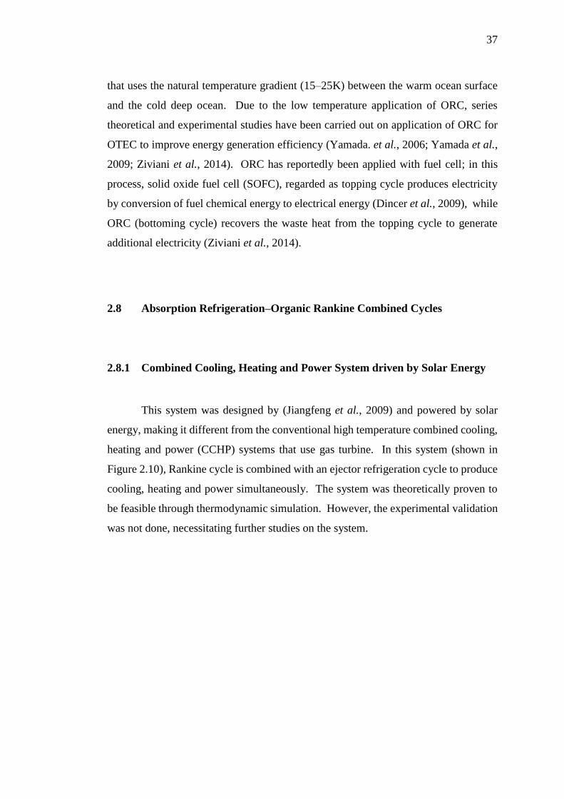
37
that uses the natural temperature gradient (15–25K) between the warm ocean surface
and the cold deep ocean. Due to the low temperature application of ORC, series
theoretical and experimental studies have been carried out on application of ORC for
OTEC to improve energy generation efficiency (Yamada. et al., 2006; Yamada et al.,
2009; Ziviani et al., 2014). ORC has reportedly been applied with fuel cell; in this
process, solid oxide fuel cell (SOFC), regarded as topping cycle produces electricity
by conversion of fuel chemical energy to electrical energy (Dincer et al., 2009), while
ORC (bottoming cycle) recovers the waste heat from the topping cycle to generate
additional electricity (Ziviani et al., 2014).
2.8 Absorption Refrigeration–Organic Rankine Combined Cycles
2.8.1 Combined Cooling, Heating and Power System driven by Solar Energy
This system was designed by (Jiangfeng et al., 2009) and powered by solar
energy, making it different from the conventional high temperature combined cooling,
heating and power (CCHP) systems that use gas turbine. In this system (shown in
Figure 2.10), Rankine cycle is combined with an ejector refrigeration cycle to produce
cooling, heating and power simultaneously. The system was theoretically proven to
be feasible through thermodynamic simulation. However, the experimental validation
was not done, necessitating further studies on the system.
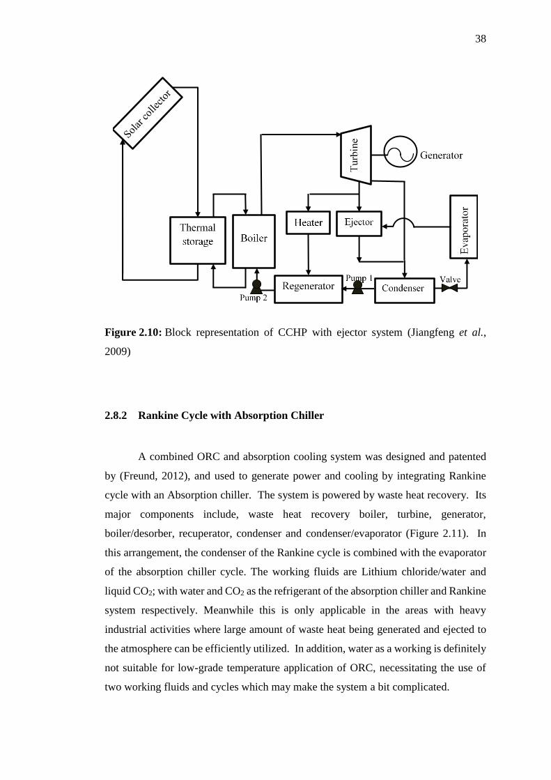
38
Figure 2.10: Block representation of CCHP with ejector system (Jiangfeng et al.,
2009)
2.8.2 Rankine Cycle with Absorption Chiller
A combined ORC and absorption cooling system was designed and patented
by (Freund, 2012), and used to generate power and cooling by integrating Rankine
cycle with an Absorption chiller. The system is powered by waste heat recovery. Its
major components include, waste heat recovery boiler, turbine, generator,
boiler/desorber, recuperator, condenser and condenser/evaporator (Figure 2.11). In
this arrangement, the condenser of the Rankine cycle is combined with the evaporator
of the absorption chiller cycle. The working fluids are Lithium chloride/water and
liquid CO2; with water and CO2 as the refrigerant of the absorption chiller and Rankine
system respectively. Meanwhile this is only applicable in the areas with heavy
industrial activities where large amount of waste heat being generated and ejected to
the atmosphere can be efficiently utilized. In addition, water as a working is definitely
not suitable for low-grade temperature application of ORC, necessitating the use of
two working fluids and cycles which may make the system a bit complicated.
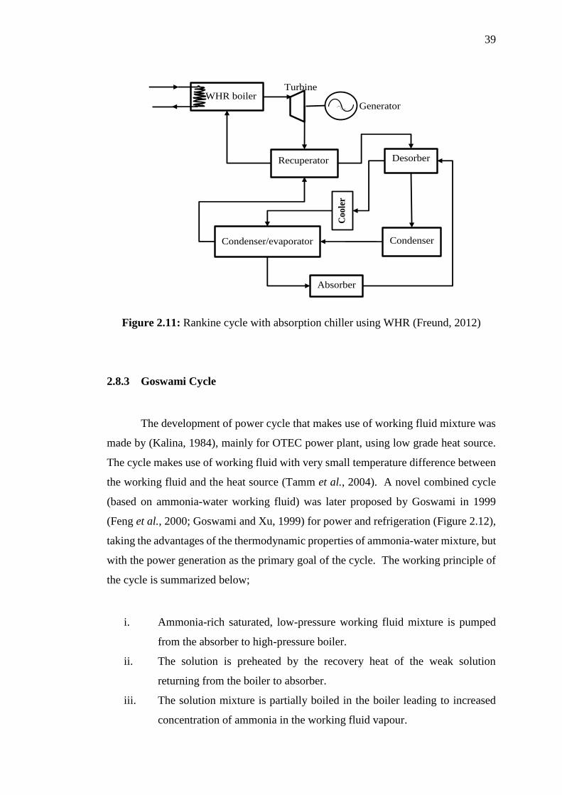
39
Figure 2.11: Rankine cycle with absorption chiller using WHR (Freund, 2012)
2.8.3 Goswami Cycle
The development of power cycle that makes use of working fluid mixture was
made by (Kalina, 1984), mainly for OTEC power plant, using low grade heat source.
The cycle makes use of working fluid with very small temperature difference between
the working fluid and the heat source (Tamm et al., 2004). A novel combined cycle
(based on ammonia-water working fluid) was later proposed by Goswami in 1999
(Feng et al., 2000; Goswami and Xu, 1999) for power and refrigeration (Figure 2.12),
taking the advantages of the thermodynamic properties of ammonia-water mixture, but
with the power generation as the primary goal of the cycle. The working principle of
the cycle is summarized below;
i. Ammonia-rich saturated, low-pressure working fluid mixture is pumped
from the absorber to high-pressure boiler.
ii. The solution is preheated by the recovery heat of the weak solution
returning from the boiler to absorber.
iii. The solution mixture is partially boiled in the boiler leading to increased
concentration of ammonia in the working fluid vapour.
WHR boiler
Desorber Recuperator
Condenser Condenser/evaporator
Absorber
Turbine
Coole
r
Generator

40
iv. Passing through the rectifier, ammonia vapour becomes purified by
condensing out the remaining water.
v. The pure ammonia is then superheated and expanded through the turbine
to produce work.
vi. The expansion in the turbine leads to reduction in ammonia temperature
thereby making it suitable for heat extraction (refrigeration) before being
absorbed by the water in the absorber tank.
Figure 2.12: Goswami combined power and refrigeration cycle (Wang et al., 2016)
Goswami cycle has been investigated by researchers (Xu. and Goswami, 1999),
using low-grade solar collector and geothermal energy respectively to drive the cycle.
Parametric analysis of the cycle had been carried out to improve both the turbine
efficiency and cooling performance of the cycle (Padilla et al., 2010). Experimental
investigations were carried out by (Tamm et al., 2004) for the validation of Goswami
cycle and it was found out that the results of the test data were in agreement with the
theoretical simulations results. Meanwhile, Goswami cycle is reported to produce low
cooling effect (Padilla et al., 2010; Wang et al., 2016) because refrigeration effect
Super heater Boiler
Turbine
Refrigeration H.E
Absorber
Recovery
H.E
Rectifier
Generator
Valve Pump

41
relies only on the pressure reduction caused by turbine expansion. It is most desirable
when the chilled water temperature around (or just below) ambient temperature is
needed. It is also observed that chilled water production is not the primary target/goal
in the Goswami cycle in which case, the inclusion of the refrigeration cycle is also
primarily to improve the efficiency of the power cycle (Xu. et al., 2000). Therefore to
have better cooling effects (where chilled water is primary and power is additional
goal), there is need for further expansion of the exhaust refrigerant vapour from the
turbine. This study did not only introduce further ammonia expansion, but also
reduced the complexity in the design, by non-inclusion of the superheater (since power
generation is a complementary requirement).
2.8.4 Chilled Water Piping and Flow Rates
In HVAC system, and specifically cooling system, chilled water network plays
an important role. Cooling is achieved by distribution of chilled water throughout the
conditioned space via the network of pipes connecting the HVAC equipment with the
space being conditioned. Therefore, efficient use of chilled water through pipe design
and optimal flow rate are important in chilled water application for cooling system.
Optimization of design and synthesis of chilled water network was proposed by (Lee
et al., 2013) which wasن alsoن demonstratedنwithن twoن caseن studiesن conductedن onن “aن
Malaysian wafer fabrication foundry”نandن“aنTaiwaneseنwaferن fabricationنfacility”.
Future study was suggested on the investigation of interaction between the chiller unit
and chilled water network systems. There are a number of studies on the chilled water
network design for cooling system (Miyazaki and Akisawa, 2009; Chen and Xu, 2012;
Liu et al., 2012).
Chilled water pumping has always been considered on three main
configurations (Hubbard, 2011), although these may not be given a detailed
explanation in this research. The configurations include;
i. Constant primary flow (CPF) system,
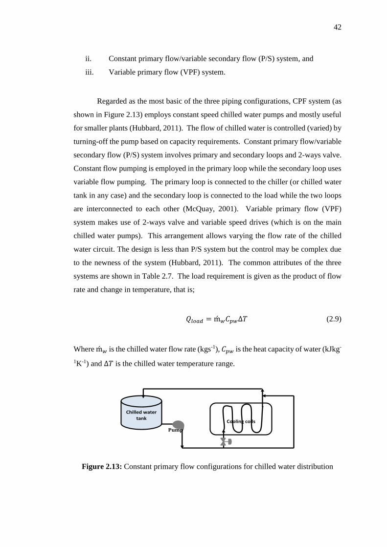
42
ii. Constant primary flow/variable secondary flow (P/S) system, and
iii. Variable primary flow (VPF) system.
Regarded as the most basic of the three piping configurations, CPF system (as
shown in Figure 2.13) employs constant speed chilled water pumps and mostly useful
for smaller plants (Hubbard, 2011). The flow of chilled water is controlled (varied) by
turning-off the pump based on capacity requirements. Constant primary flow/variable
secondary flow (P/S) system involves primary and secondary loops and 2-ways valve.
Constant flow pumping is employed in the primary loop while the secondary loop uses
variable flow pumping. The primary loop is connected to the chiller (or chilled water
tank in any case) and the secondary loop is connected to the load while the two loops
are interconnected to each other (McQuay, 2001). Variable primary flow (VPF)
system makes use of 2-ways valve and variable speed drives (which is on the main
chilled water pumps). This arrangement allows varying the flow rate of the chilled
water circuit. The design is less than P/S system but the control may be complex due
to the newness of the system (Hubbard, 2011). The common attributes of the three
systems are shown in Table 2.7. The load requirement is given as the product of flow
rate and change in temperature, that is;
𝑄𝑙𝑜𝑎𝑑 = ḿ𝑤𝐶𝑝𝑤∆𝑇 (2.9)
Where ḿ𝑤 is the chilled water flow rate (kgs-1), 𝐶𝑝𝑤 is the heat capacity of water (kJkg-
1K-1) and ∆𝑇 is the chilled water temperature range.
Figure 2.13: Constant primary flow configurations for chilled water distribution
Chilled water tank
Cooling coils
Pump
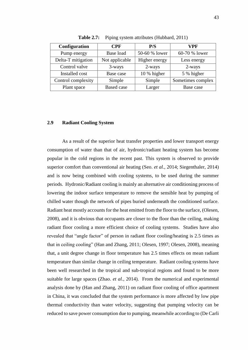
43
Table 2.7: Piping system attributes (Hubbard, 2011)
Configuration CPF P/S VPF
Pump energy Base load 50-60 % lower 60-70 % lower
Delta-T mitigation Not applicable Higher energy Less energy
Control valve 3-ways 2-ways 2-ways
Installed cost Base case 10 % higher 5 % higher
Control complexity Simple Simple Sometimes complex
Plant space Based case Larger Base case
2.9 Radiant Cooling System
As a result of the superior heat transfer properties and lower transport energy
consumption of water than that of air, hydronic/radiant heating system has become
popular in the cold regions in the recent past. This system is observed to provide
superior comfort than conventional air heating (Seo. et al., 2014; Siegenthaler, 2014)
and is now being combined with cooling systems, to be used during the summer
periods. Hydronic/Radiant cooling is mainly an alternative air conditioning process of
lowering the indoor surface temperature to remove the sensible heat by pumping of
chilled water though the network of pipes buried underneath the conditioned surface.
Radiant heat mostly accounts for the heat emitted from the floor to the surface, (Olesen,
2008), and it is obvious that occupants are closer to the floor than the ceiling, making
radiant floor cooling a more efficient choice of cooling systems. Studies have also
revealedنthatن“angleنfactor” of person in radiant floor cooling/heating is 2.5 times as
thatنinنceilingنcooling”ن(Han and Zhang, 2011; Olesen, 1997; Olesen, 2008), meaning
that, a unit degree change in floor temperature has 2.5 times effects on mean radiant
temperature than similar change in ceiling temperature. Radiant cooling systems have
been well researched in the tropical and sub-tropical regions and found to be more
suitable for large spaces (Zhao. et al., 2014). From the numerical and experimental
analysis done by (Han and Zhang, 2011) on radiant floor cooling of office apartment
in China, it was concluded that the system performance is more affected by low pipe
thermal conductivity than water velocity, suggesting that pumping velocity can be
reduced to save power consumption due to pumping, meanwhile according to (De Carli
44
and Tonon, 2011) the radiant floor cooling performance depends more on the thickness
and thermal conductivity of the material in which the cooling pipe (tube) is embedded.
Furthermore, ground-source heat pump (GSHP) has been extensively applied
for soil cooling process where heat removal is achieved through the embedded heat
exchanger pipe (earth tube) that transfers heat between the soil and GSHP (Moncef
and Kreider, 1996; Demir et al., 2009). Design of solar thermal cooling system was
done by (Kalkan et al., 2012), which is to be integrated into present and future
residential apartments. Further study on their work was suggested to include
integration of GSHP system with the building so that soil can act as heat sink for
cooling the building. Various studies have been focused on radiant cooling systems
especially in large spaces with moderate-to-high occupancy density (Mikeska. and
Svendsen, 2015). Zhao, in (Zhao. et al., 2015) studied the prediction of radiant floor
coolingنcapacityنofنlargeنspaces,نusingنXi’anن Xianyang international airport in China
as a case study to find out the extent of transient solar radiation effect on the cooling
capacity of radiant floor cooling system. In the earlier study, they (Zhao. et al., 2014)
did analysis of solar radiation effects on the capacity of radiant floor cooling in the
same airport, based on ‘on-site performance measurement’. Experimental field study
and comfort assessment of radiant cooling of residential building in tropical Thailand
was done by (Wattanakit. et al., 2014; Wongkee. et al., 2014b). The study revealed
that radiant cooling together with dehumidification is able to improve the thermal
comfort of the studied space, with the achievement of about 70 % energy savings
compared with the conventional air conditioning system. However, dehumidification
was suggested to avoid surface condensation of the cooled inner wall, or alternatively
the cooled surface temperature could be kept above the dew point (Ahmed and
Medhat, 2012). All these studies and applications point to the better performance of
chilled water for cooling application than chilled air systems and most importantly for
soil/floor cooling systems.
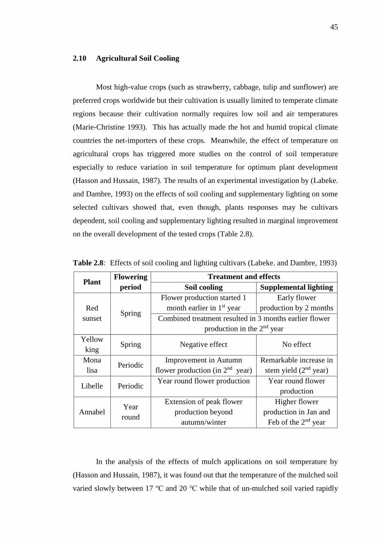
45
2.10 Agricultural Soil Cooling
Most high-value crops (such as strawberry, cabbage, tulip and sunflower) are
preferred crops worldwide but their cultivation is usually limited to temperate climate
regions because their cultivation normally requires low soil and air temperatures
(Marie-Christine 1993). This has actually made the hot and humid tropical climate
countries the net-importers of these crops. Meanwhile, the effect of temperature on
agricultural crops has triggered more studies on the control of soil temperature
especially to reduce variation in soil temperature for optimum plant development
(Hasson and Hussain, 1987). The results of an experimental investigation by (Labeke.
and Dambre, 1993) on the effects of soil cooling and supplementary lighting on some
selected cultivars showed that, even though, plants responses may be cultivars
dependent, soil cooling and supplementary lighting resulted in marginal improvement
on the overall development of the tested crops (Table 2.8).
Table 2.8: Effects of soil cooling and lighting cultivars (Labeke. and Dambre, 1993)
Plant Flowering
period
Treatment and effects
Soil cooling Supplemental lighting
Red
sunset Spring
Flower production started 1
month earlier in 1st year
Early flower
production by 2 months
Combined treatment resulted in 3 months earlier flower
production in the 2nd year
Yellow
king Spring Negative effect No effect
Mona
lisa Periodic
Improvement in Autumn
flower production (in 2nd year)
Remarkable increase in
stem yield (2nd year)
Libelle Periodic Year round flower production Year round flower
production
Annabel Year
round
Extension of peak flower
production beyond
autumn/winter
Higher flower
production in Jan and
Feb of the 2nd year
In the analysis of the effects of mulch applications on soil temperature by
(Hasson and Hussain, 1987), it was found out that the temperature of the mulched soil
varied slowly between 17 ℃ and 20 ℃ while that of un-mulched soil varied rapidly
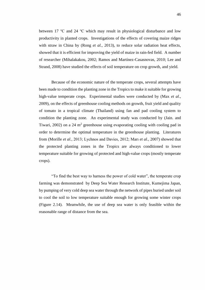
46
between 17 ℃ and 24 ℃ which may result in physiological disturbance and low
productivity in planted crops. Investigations of the effects of covering maize ridges
with straw in China by (Rong et al., 2013), to reduce solar radiation heat effects,
showed that it is efficient for improving the yield of maize in rain-fed field. A number
of researcher (Mihalakakou, 2002; Ramos and Martínez-Casasnovas, 2010; Lee and
Strand, 2008) have studied the effects of soil temperature on crop growth, and yield.
Because of the economic nature of the temperate crops, several attempts have
been made to condition the planting zone in the Tropics to make it suitable for growing
high-value temperate crops. Experimental studies were conducted by (Max et al.,
2009), on the effects of greenhouse cooling methods on growth, fruit yield and quality
of tomato in a tropical climate (Thailand) using fan and pad cooling system to
condition the planting zone. An experimental study was conducted by (Jain. and
Tiwari, 2002) on a 24 m2 greenhouse using evaporating cooling with cooling pad in
order to determine the optimal temperature in the greenhouse planting. Literatures
from (Morille et al.,ن;2013نLychnosنandنDavies,ن;2012نMarı et al., 2007) showed that
the protected planting zones in the Tropics are always conditioned to lower
temperature suitable for growing of protected and high-value crops (mostly temperate
crops).
“Toنfindنtheنbestنwayنtoنharnessنtheنpowerنofنcoldنwater”,نtheنtemperateنcropن
farming was demonstrated by Deep Sea Water Research Institute, Kumejima Japan,
by pumping of very cold deep sea water through the network of pipes buried under soil
to cool the soil to low temperature suitable enough for growing some winter crops
(Figure 2.14). Meanwhile, the use of deep sea water is only feasible within the
reasonable range of distance from the sea.
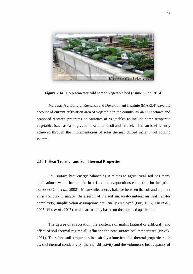
47
Figure 2.14: Deep seawater cold season vegetable bed (KumeGuide, 2014)
Malaysia Agricultural Research and Development Institute (MARDI) gave the
account of current cultivation area of vegetable in the country as 44000 hectares and
proposed research programs on varieties of vegetables to include some temperate
vegetables (such as cabbage, cauliflower, broccoli and lettuce). This can be efficiently
achieved through the implementation of solar thermal chilled radiant soil cooling
system.
2.10.1 Heat Transfer and Soil Thermal Properties
Soil surface heat energy balance as it relates to agricultural soil has many
applications, which include the heat flux and evaporations estimation for irrigation
purposes (Qin et al., 2002). Meanwhile, energy balance between the soil and ambient
air is complex in nature. As a result of the soil surface-to-ambient air heat transfer
complexity, simplification assumptions are usually employed (Puri, 1987; Liu et al.,
2005; Wu. et al., 2015), which are usually based on the intended application.
The degree of evaporation, the existence of mulch (natural or artificial), and
effect of soil thermal regime all influence the near surface soil temperature (Novak,
1981). Therefore, soil temperature is basically a function of its thermal properties such
as; soil thermal conductivity, thermal diffusivity and the volumetric heat capacity of

48
the soil as well as amount of heat transfer to the soil (majorly from solar radiation).
Soil thermal conductivity (Ks), in a simpler form, is the heat flux through the soil
divided by the change in temperature along the heat flux. The thermal conductivity of
soil (Wm−1K−1) is influenced by compactness of the soil and its moisture contents
(Demir et al., 2009; De Carli and Tonon, 2011). Thermal diffusivity on the other hand
is the temperature change resulting from flow of a unit quantity of heat through a unit
volume per unit time (m2𝑠−1). Volumetric heat capacity (kJm-3K-1) of soil is its ability
to store heat energy during change in temperature. The three properties are related as;
∝=𝑘
𝜌𝐶𝑝 (2.10)
Where ∝ is the diffusivity (𝑚2𝑠−1), 𝑘 is the thermal conductivity (𝑊𝑚−1𝐾−1), 𝜌 is
the soil density (𝐾𝑔𝑚−3) and 𝐶𝑝 is the specific heat capacity of the soil. The term 𝜌𝐶𝑝
is the volumetric heat capacity of the soil.
However, this study is not intended to go into more details on the soil heat
transfer but only as it relates to soil heat exchange due solar radiation absorbed by the
soil and the transfer of such heat between the soil surface and the buried chilled water
pipe.
2.11 Economic Analysis
Decision making on systems design requires more than just the thermodynamic
analysis and optimization of the system, as such more attention is being paid to the
system economic analysis (Wang et al., 2016). Particularly, decision making on
Renewable Energy Technology (RET) projects is a complex task that requires the
determination of the technically feasible technology, the energy efficiency index, as
well as the economic efficiency of the potential project. Meanwhile, the decision must
be made at the initial stages of the project which in most cases are new or unfamiliar
projects. RETScreen® software is a unique decision support tool, designed to address

49
this kind of problems. It is a tool that can quickly analyse and evaluate the viability of
one or more renewable energy technology options at the initial stage of the project
(Ackom, 2005). RETScreen® was developed by the Natural Resources Canada (NRC)
with contributions from about 85 experts and organizations including the United
Nations Environment Program (UNEP) and the National Aeronautics & Space
Management (NASA) to provide international weather data base (RETScreen, 2005).
The software runs on Microsoft excel and it is suitably useful for evaluation of energy
production and savings, costs, emissions reductions, financial viability, life cycle cost,
and risk assessment of different types of Energy efficient and Renewable Energy
Technologies. RETScreen has been used by researchers (Lee et al., 2012; Tarigan et
al., 2015; Duggirala, 2010; Ackom, 2005) for feasibility and viability studies of
renewable energy projects and energy efficient technologies. The software is a
stepwise modelling tool (as shown in Figure 2.15), in which each of the steps is
associated with Excel worksheet. The software usually analyses renewable energy
project by comparing its financial and emission details with a base case (using other
energy sources).
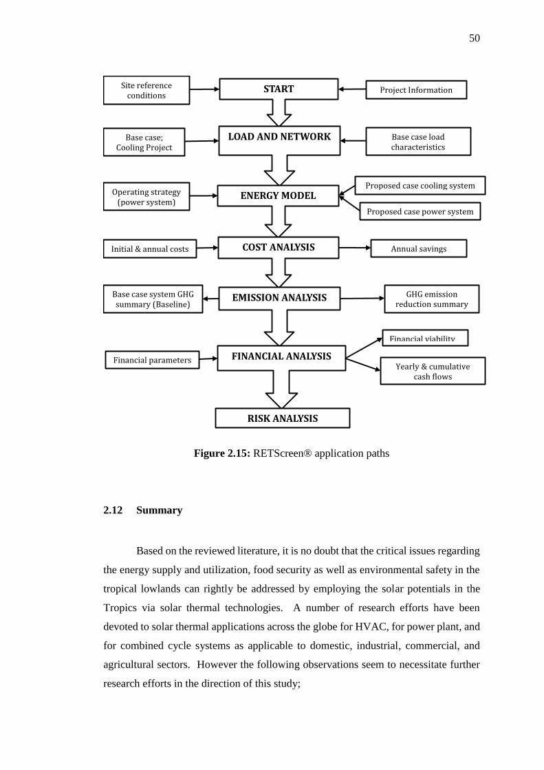
50
Figure 2.15: RETScreen® application paths
2.12 Summary
Based on the reviewed literature, it is no doubt that the critical issues regarding
the energy supply and utilization, food security as well as environmental safety in the
tropical lowlands can rightly be addressed by employing the solar potentials in the
Tropics via solar thermal technologies. A number of research efforts have been
devoted to solar thermal applications across the globe for HVAC, for power plant, and
for combined cycle systems as applicable to domestic, industrial, commercial, and
agricultural sectors. However the following observations seem to necessitate further
research efforts in the direction of this study;
Project Information
Base case; Cooling Project
Proposed case cooling system
Annual savings
Initial & annual costs
Base case system GHG summary (Baseline)
GHG emission reduction summary
Financial parameters
Financial viability
Site reference conditions
Base case load characteristics
Yearly & cumulative cash flows
Proposed case power system
Operating strategy (power system)

51
i. Most of the soil or floor cooling applications reviewed were achieved
through circulation of chilled air; a more energy consuming process than
chilled water. However, few of that chilled water applications for radiant
cooling were mainly obtained from the grid-electricity powered cooling
system.
ii. Most combined power and cooling plants in the literature operating on low-
to-medium grade heat use separate cycles and separate sets of working fluid
for the power and cooling therefore making the plant design a little bit
complex.
iii. For the combined power and cooling cycles that operated on one cycle and
one set of working fluid, power generation formed the primary goal and
cooling was secondary; as such, the temperatures of chilled water
obtainable from such cycles were just a bit below the ambient temperature
and might not be suitable in cases whereنhigherن‘coolingنeffect’نisنrequired.

52
CHAPTER 3
3 RESEARCH METHODOLOGY
3.1 Introduction
This study is on an integrated system of a combined power and refrigeration
plant, and on a radiant soil cooling systems. The combined plant is modelled to meet
the specific requirement to overcome a radiant soil cooling load, therefore the
methodology part of this study starts with the soil heat transfer modelling to determine
theن“soilنcoolingنload”.ن This is done to have an idea of the cooling load which the
modelled combined plant must optimally provide. For the soil cooling process,
thermal properties of the soil at the project location are considered. While the heat
transfers acrossنtheن“soil–pipe–chilled water” section is modelled using properties of
soil, pipe, and chilled water, respectively. For a specified load, the equivalent
combined plant component parts are modelled to determine its overall capacity
(including the required energy input, and the effective size of the solar collector). The
thermodynamic properties of the working fluid are employed in the plant components
modelling. The modelling methodology, equations, and assumptions used are
described in details in the following parts of this chapter.
Relating the soil cooling load to the area of soil bed, gives the idea of the
approximate plant cooling capacity needed to overcome the load (and vice versa), and
the length of the chilled water pipe required to circulate the cooling effect.
Computer programming algorithm and codes are developed for the
implementation of the calculations involved in the models. The modelled system is
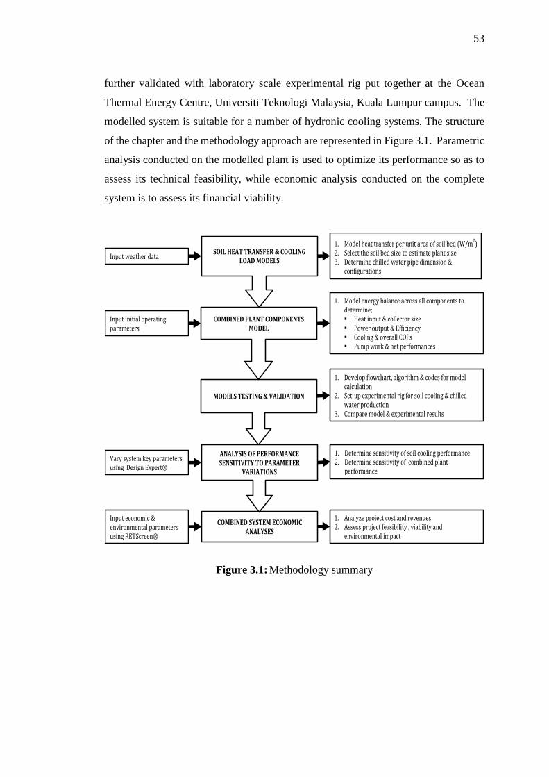
53
further validated with laboratory scale experimental rig put together at the Ocean
Thermal Energy Centre, Universiti Teknologi Malaysia, Kuala Lumpur campus. The
modelled system is suitable for a number of hydronic cooling systems. The structure
of the chapter and the methodology approach are represented in Figure 3.1. Parametric
analysis conducted on the modelled plant is used to optimize its performance so as to
assess its technical feasibility, while economic analysis conducted on the complete
system is to assess its financial viability.
Figure 3.1: Methodology summary
SOIL HEAT TRANSFER & COOLING LOAD MODELS
COMBINED PLANT COMPONENTS MODEL
ANALYSIS OF PERFORMANCE SENSITIVITY TO PARAMETER
VARIATIONS
COMBINED SYSTEM ECONOMIC ANALYSES
MODELS TESTING & VALIDATION
1. Model heat transfer per unit area of soil bed (W/m2)
2. Select the soil bed size to estimate plant size
3. Determine chilled water pipe dimension & configurations
1. Model energy balance across all components to determine; Heat input & collector size
Power output & Efficiency
Cooling & overall COPs
Pump work & net performances
Input weather data
1. Develop flowchart, algorithm & codes for model calculation
2. Set-up experimental rig for soil cooling & chilled water production
3. Compare model & experimental results
1. Determine sensitivity of soil cooling performance
2. Determine sensitivity of combined plant performance
Input economic & environmental parameters using RETScreen®
1. Analyze project cost and revenues
2. Assess project feasibility , viability and environmental impact
Input initial operating parameters
Vary system key parameters, using Design Expert®
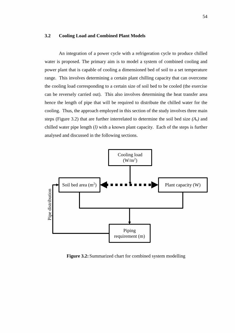
54
3.2 Cooling Load and Combined Plant Models
An integration of a power cycle with a refrigeration cycle to produce chilled
water is proposed. The primary aim is to model a system of combined cooling and
power plant that is capable of cooling a dimensioned bed of soil to a set temperature
range. This involves determining a certain plant chilling capacity that can overcome
the cooling load corresponding to a certain size of soil bed to be cooled (the exercise
can be reversely carried out). This also involves determining the heat transfer area
hence the length of pipe that will be required to distribute the chilled water for the
cooling. Thus, the approach employed in this section of the study involves three main
steps (Figure 3.2) that are further interrelated to determine the soil bed size (As) and
chilled water pipe length (l) with a known plant capacity. Each of the steps is further
analysed and discussed in the following sections.
Figure 3.2: Summarized chart for combined system modelling
Cooling load
(W/m2)
Plant capacity (W)
Piping
requirement (m)
Soil bed area (m2)
Pip
e dis
trib
uti
on

55
3.2.1 Soil Heat Transfer and Cooling Load Models
In this section, the heat transfer between the homogeneous soil structure and
the ambient environment (under the influence of solar radiation) is considered together
with the net transfer occurring as a result of the temperature difference between bulk
soil and the chilled water in the pipe (buried under the soil). The summaries of the soil
heat transfer processes are listed in a stepwise approach below, with illustration in
Figure 3.3.
Figure 3.3: Heat transfer model
i. Modelling of ground (soil) surface heat transfer: that is, heat transfer
resulting from the temperature difference between the bare soil surface and
the ambient environment under the influence of solar radiation;
ii. Modelling of the vertical heat conduction from the soil surface down to the
buried chilled water pipe;
iii. Modelling of heat gained by the chilled water by conduction through the
pipe wall followed by convection from pipe inner surface of the pipe to the
flowing water.
Bare Soil surface
Absorbed incident
solar radiation
Sensible heat
flux from soil
Latent heat flux due
to evaporation
Vertical heat conduction through the soil
Chilled water tube
Convection heat transfer between inner surface of the tube to flowing water
Conductive heat through the tube wall
Conductive heat from soil envelope to the outer tube wall
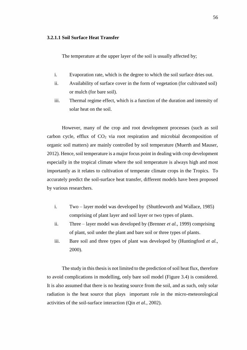
56
3.2.1.1 Soil Surface Heat Transfer
The temperature at the upper layer of the soil is usually affected by;
i. Evaporation rate, which is the degree to which the soil surface dries out.
ii. Availability of surface cover in the form of vegetation (for cultivated soil)
or mulch (for bare soil).
iii. Thermal regime effect, which is a function of the duration and intensity of
solar heat on the soil.
However, many of the crop and root development processes (such as soil
carbon cycle, efflux of CO2 via root respiration and microbial decomposition of
organic soil matters) are mainly controlled by soil temperature (Muerth and Mauser,
2012). Hence, soil temperature is a major focus point in dealing with crop development
especially in the tropical climate where the soil temperature is always high and most
importantly as it relates to cultivation of temperate climate crops in the Tropics. To
accurately predict the soil-surface heat transfer, different models have been proposed
by various researchers.
i. Two – layer model was developed by (Shuttleworth and Wallace, 1985)
comprising of plant layer and soil layer or two types of plants.
ii. Three – layer model was developed by (Brenner et al., 1999) comprising
of plant, soil under the plant and bare soil or three types of plants.
iii. Bare soil and three types of plant was developed by (Huntingford et al.,
2000).
The study in this thesis is not limited to the prediction of soil heat flux, therefore
to avoid complications in modelling, only bare soil model (Figure 3.4) is considered.
It is also assumed that there is no heating source from the soil, and as such, only solar
radiation is the heat source that plays important role in the micro-meteorological
activities of the soil-surface interaction (Qin et al., 2002).
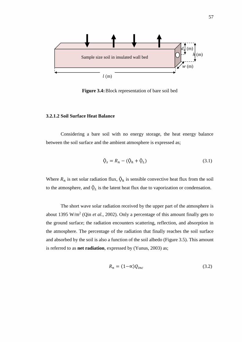
57
Figure 3.4: Block representation of bare soil bed
3.2.1.2 Soil Surface Heat Balance
Considering a bare soil with no energy storage, the heat energy balance
between the soil surface and the ambient atmosphere is expressed as;
Ǭ𝑠 = 𝑅𝑛 − (Ǭℎ + Ǭ𝐿) (3.1)
Where 𝑅𝑛 is net solar radiation flux, Ǭℎ is sensible convective heat flux from the soil
to the atmosphere, and Ǭ𝐿 is the latent heat flux due to vaporization or condensation.
The short wave solar radiation received by the upper part of the atmosphere is
about 1395 W/m2 (Qin et al., 2002). Only a percentage of this amount finally gets to
the ground surface; the radiation encounters scattering, reflection, and absorption in
the atmosphere. The percentage of the radiation that finally reaches the soil surface
and absorbed by the soil is also a function of the soil albedo (Figure 3.5). This amount
is referred to as net radiation, expressed by (Yunus, 2003) as;
𝑅𝑛 = (1−∝)𝑄𝑖𝑛𝑐 (3.2)
Sample size soil in insulated wall bed
(m)
ℎ (m)
(m)
(m)

58
Figure 3.5: Solar radiations on bare soil surface
With respect to Stefan-Boltzmann law, the net radiation absorbed by bare soil
is expressed as;
𝑅𝑛 = (1−∝)𝑄𝑖𝑛𝑐 + 𝜎ℇ𝑠(ℇ𝑎𝑇𝑎4 − 𝑇𝑠
4) (3.3)
Where 𝑄𝑖𝑛𝑐 is incident solar radiation on the soil (W/m2), ∝ is the soil surface albedo,
𝜎 is the Boltzmann constant, ℇ𝑠 & ℇ𝑎 are soil and air emissivities, and 𝑇𝑠 & 𝑇𝑎 are the
respective temperatures at the soil surface and air.
The ground surface–ambient air temperature difference always results in
sensible heat transfer (Ǭ𝒉) between the two sides. This is also affected by the
resistance of the surface to heat transfer (𝑟𝑎). The sensible heat flux from the soil to the
atmosphere (or vice versa) is given by (Novak, 2010; Qin et al., 2002) as;
Ǭℎ =𝜌𝑎𝐶𝑝𝑎(𝑇0−𝑇𝑎)
𝑟𝑎 (3.4)
And the surface resistance to the heat flux (𝑟𝑎) is expressed as;
𝑟𝑎 =ln (𝑍𝑟−
𝑑
𝑍0)2
𝐾2𝑈𝑟 (Liu et al., 2007; Villagarcía et al., 2007; Qin et al., 2002)
(3.5)
Where 𝜌𝑎is density of air above the soil, 𝐶𝑝𝑎 is specific heat of air (at constant
pressure), 𝑟𝑎 is boundary layer resistance (sm-1), 𝑍𝑟 is the reference height, d is 0 for
= (1−∝)
=∝

59
bare soil (Liu et al., 2007; Novak, 2010), 𝑈𝑟 is the wind speed, 𝐾 is Van Karman
constant.
Energy exchange due to evaporation or condensation between the ground
surface and the atmosphere is a function of moisture availability in the atmosphere
(Muerth and Mauser, 2012). The energy required for the evaporation is regarded as
latent heat flux Ǭ𝑳 and is given as;
Ǭ𝐿 = 𝜌𝑤𝑞𝑙𝐸 (3.6)
𝐸 =𝜌𝑣0−𝜌𝑣𝑎
𝑟𝑎𝜌𝑤 (Novak, 2010) (3.7)
𝜌𝑣0(𝑡) = 𝜌𝑣∗(𝑇)ℎ𝑟 = [
1.323
𝑇𝑒(
17.27𝑇−4717.3
𝑇−35.85)]ℎ𝑟 (Tetëns, 1930) modified by
(Novak, 2010).
𝜌𝑣𝑎(𝑡) =𝑒𝑎(𝑡)𝑀𝑤
𝑅𝑇𝑎(𝑡) (Novak 1981)
Therefore, the net heat energy absorbed at the surface of dimensioned soil bed
in this case, is expressed as;
Ǭ𝑠 = 𝑅𝑛 − (Ǭℎ + Ǭ𝐿)𝐴𝑠 (3.8)
Where 𝜌𝑣0 is soil surface vapour density, 𝜌𝑣𝑎
water vapour density at reference height,
ℎ𝑟 is height of soil surface roughness, 𝑒𝑎(𝑡) is water vapour pressure at reference
height, 𝑀𝑤 is molar mass of water, and R is the ideal gas constant, 𝐴𝑠 is the surface
area of the soil bed.

60
3.2.1.3 Soil Cooling Load
With reference to (ASHRAE, 2009), cooling load calculation helps to
determine the total sensible cooling load resulting from heat gained through;
i. Opaque surfaces such as walls, floors, ceilings, and doors;
ii. Transparent fenestration surfaces such as windows, skylights, and glazed
doors;
iii. Infiltration and ventilation;
iv. Occupancy effects;
Opaque body in the above refers to heat gained resulting from the temperature
difference across surfaces or solar gain incident on the surface. In this study, the
cooling load of interest falls in the first category (solar gain incident on the surface)
since a bare soil is being considered in the model. Meanwhile, it is a common practice
in load design to always consider uncertainties that may arise from service conditions
or load variations (Moser and Folkman, 2008). This is usually taken care of by ‘factor
of safety’ which is used either to allow future growth in loads so that the equipment
can operate within the safe range (Sharizal, 2006) , or to reduce the possibility of
oversizing or under-sizing of HVAC equipment (Parameshwaran et al., 2012).
Therefore the cooling load in this study is calculated as the product of the net heat flux
on the soil and a safety factor, given as;
Ǭ𝑙𝑜𝑎𝑑 = Ǭ𝑠 × 𝛾 (3.9)
Where 𝛾 is the factor of safety, and Ǭ𝑠 is the net heat flux on the soil.
3.2.1.4 Vertical Heat Conduction
Conductive heat transfer in soil is considered as the net exchange of kinetic
energy by the soil molecules. This usually occurs from a higher temperature (hot)

61
region to the lower temperature (cold) region (Muerth and Mauser, 2012; Rose, 1969).
In this study, the soil surface is the hot region while the external surface of the chilled
water pipe is the cold region. However, researches by (Moncef and Kreider, 1996) and
(Novak, 1981) have shown that at any given depth (z) below the surface, the
undisturbed ground (soil) temperature (𝑇𝑠𝑢) follows a periodical/harmonic variation
with time and the expression can simply be put as;
𝑇𝑠𝑢(𝑧, 𝑡) = 𝑇𝑚 + 𝑇𝑎𝑚𝑅𝑒(𝑒𝑖𝑤𝑡) (3.10)
This is in consonance with the earlier study conducted by (Kusuda and
Archenbach, 1965) as reported by (Moncef and Kreider, 1996) with reference to
undisturbed soil temperature around chilled water tube.
The heat conduction from the top soil to the chilled water tube can be expressed
using the Fourier heat conduction equation. The vertical heat flux due to conduction
depends largely on the temperature gradient through the conducting depth, and the
thermal conductivity of the soil through which the conduction is taking place (Muerth
and Mauser, 2012). Thus, in the absence of temperature gradient, conduction process
decays.
Ǭ𝑐𝑜𝑛𝑑 = −𝑘𝑠∆𝑇
∆𝑍𝐴𝑠 (3.11)
However, heat conduction through a homogeneous layer (𝑧𝑖 𝑎𝑛𝑑 𝑧𝑖+1) is a
function of the depth and time (Muerth and Mauser, 2012). Therefore;
Ǭ𝑐𝑜𝑛𝑑(𝑖,𝑖+1) = −𝑘𝑠(𝑖)
∆𝑇𝑖(𝑡)
∆𝑍𝑖𝐴𝑠
In this study, conduction heat transfer analysis is limited to the vertical distance
between the soil surface and chilled water tube, therefore our ∆𝑍𝑖 is fixed as 𝑍, and the
transfer considered with respect to time is given as;

62
Ǭ𝑐𝑜𝑛𝑑(𝑡) = −𝑘𝑠∆𝑇𝑠
𝑢(𝑡)
𝑍𝐴𝑠 (3.12)
Where 𝑘𝑠 is the soil thermal conductivity, 𝐴𝑠 is the surface area of the soil bed and ∆𝑍
is the vertical depth between the top soil and the chilled water pipe, 𝑇𝑠𝑢is the
undisturbed soil temperature, 𝑇𝑚 & 𝑇𝑎𝑚 are mean and amplitude of the ground surface
temperature variations, 𝑤 is the angular frequency of the periodic variation (𝑤 =
2𝜋/𝑑𝑎𝑦).
3.2.1.5 Chilled Water–Soil Heat Transfer
Soil cooling process is achieved through the heat transfer from the soil bed,
across the chilled water pipe network (earth tube), to the chilled water flowing through
the pipe. This heat transfer equals to the amount of heat gained by the chilled water as
it flows along the earth tube. Figure 3.6 shows the modelling sequence for the heat
transfer processes. However, the processes occurring around the earth tube is usually
complex (Lee. and Strand, 2006), hence some assumptions made to reduce the
complexities include;
i. The soil surrounding the earth tube is assumed homogeneous with constant
thermal conductivity.
ii. The temperatures of the soil in contact with the earth tube and that of earth
tube external wall are assumed equal.
iii. The presence of the earth tube has no effect on the temperature profile of
the immediate surrounding soil, hence, the temperature at the surface of the
earth tube is uniform along the axial direction (Lee and Strand, 2008).
iv. The earth tube has uniform cross sectional area in axial direction.
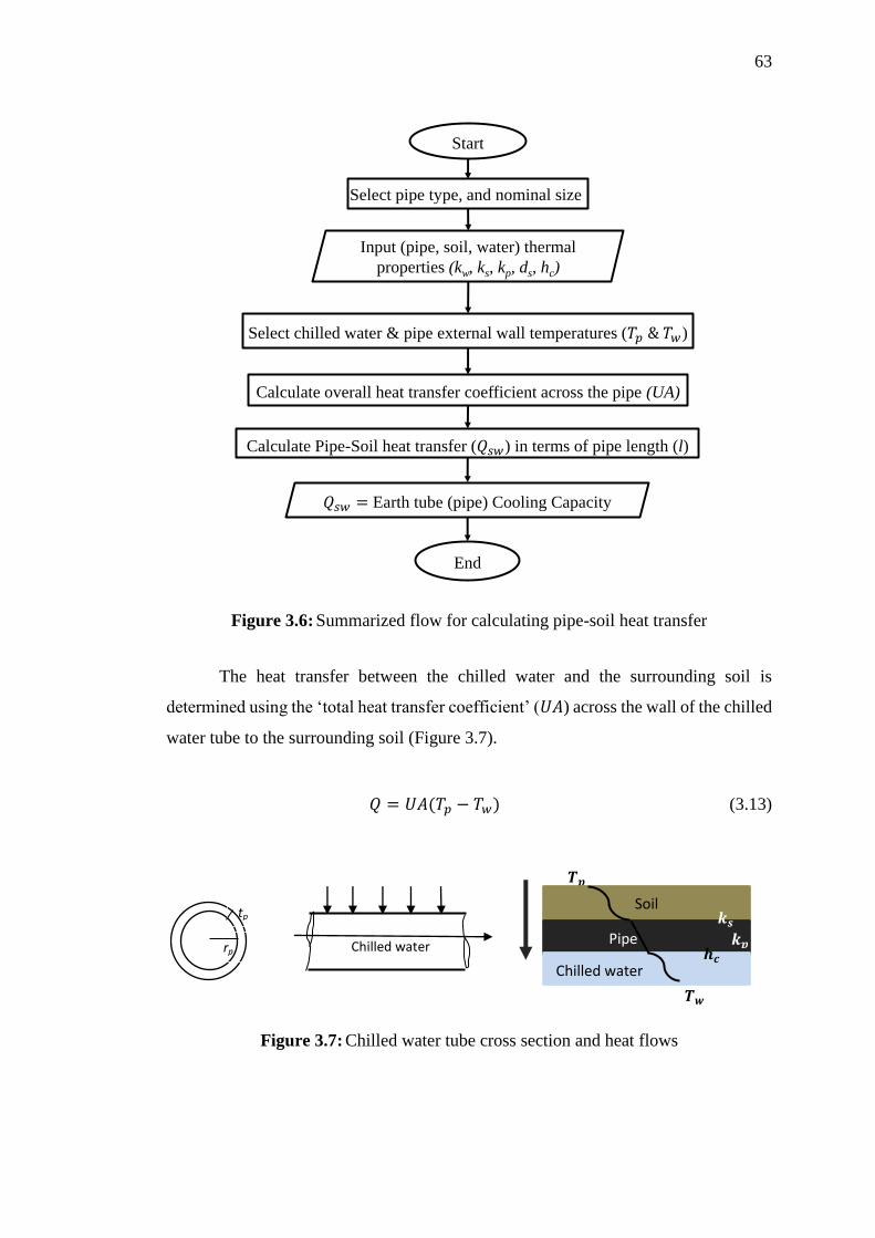
63
Figure 3.6: Summarized flow for calculating pipe-soil heat transfer
The heat transfer between the chilled water and the surrounding soil is
determinedنusingنtheن‘totalنheatنtransferنcoefficient’ن(𝑈𝐴) across the wall of the chilled
water tube to the surrounding soil (Figure 3.7).
𝑄 = 𝑈𝐴(𝑇𝑝 − 𝑇𝑤) (3.13)
Figure 3.7: Chilled water tube cross section and heat flows
Start
Select pipe type, and nominal size
Input (pipe, soil, water) thermal
properties (kw, ks, kp, ds, hc)
Select chilled water & pipe external wall temperatures ( )
Calculate overall heat transfer coefficient across the pipe (UA)
Calculate Pipe-Soil heat transfer ( ) in terms of pipe length (l)
Earth tube (pipe) Cooling Capacity
End
Chilled water rp
tp
Soil
Pipe
Chilled water

64
The overall heat transfer coefficient (𝑈𝐴) is expressed in terms of the resistance
to heat transfer across the earth tube (Lee and Strand, 2008). The resistance against
the flow of heat across the chilled water tube (to the chilled water) from the
surrounding soil (analogous to electrical resistance) is represented in Figure 3.8,
followed by the stepwise analysis of the resistance across each of the boundary layers.
Figure 3.8: Schematics of resistances to heat transfer across chilled water tube
Resistance 𝑅1 to convective heat transfer between the chilled water and the
inner surface of the tube is expressed as;
𝑅1 =1
ℎ𝐴=
1
2𝜋𝑟𝑡𝑙ℎ𝑐 (3.14)
ℎ𝑐 =𝑁𝑢𝑘𝑤
2𝑟𝑡 (Subramanian, 2008)
Resistance R2 to conductive heat transfer from the outer surface of the tube to
its inner surface is given as;
𝑅2 =1
2𝜋𝑙𝑘𝑝ln (
𝑟𝑡+𝑡𝑝
𝑟𝑡) (3.15)
Resistance R3 to conductive heat transfer between surrounding soil and the
external wall of the tube is expressed as;
𝑅3 =1
2𝜋𝑙𝑘𝑠ln (
𝑟𝑡+𝑡𝑝+𝑑𝑠
𝑟𝑡+𝑡𝑝) (3.16)
Total resistance 𝑅𝑡 is given as;
𝑅𝑡 = 𝑅1 + 𝑅2 + 𝑅3 (3.17)
65
Total heat transfer coefficient is expressed as;
𝑈𝑡 = 𝑈𝐴 =1
𝑅𝑡 (3.18)
Assuming steady flow in the system, the heat transfer between the surrounding
soil (outside the tube) and chilled water (in the tube), the net heat transfer is given as;
Ǭ𝑠𝑤 = 𝑈𝐴[𝑇𝑠 − 𝑇𝑤] (3.19)
Where ℎ𝑐 is convective heat transfer coefficient, l is the tube length, 𝑟𝑡 inner radius of
the chilled water tube, 𝑡𝑝is the tube thickness, 𝑑𝑠 is the distance between the tube
external wall and the surrounding soil, 𝑘𝑤 is the thermal conductivity of water, 𝑇𝑠& 𝑇𝑤
are the temperatures of the surrounding soil and chilled water, respectively, and 𝑁𝑢 is
Nusselt number. However, 𝑇𝑠 is assumed equal to 𝑇𝑝.
3.2.1.6 Earth Tube Material
In the HVAC system applications, radiant floor/soil cooling with chilled
water/chilled air is usually achieved through the network of pipes between the HVAC
system and the conditioned space. However, horizontal earth tube system (HETS) is
popular in radiant heat transfer between soil and buried tube with the application of a
working fluid (Mongkon et al., 2014; Lee and Strand, 2008), which is in most cases
air or water. In this study, chilled water is the working fluid through which the heat
transfer takes place.
Furthermore, the exchange off heat between the chilled water and the cooled
surface is usually determined with reference to construction parameters as well as the
difference between the temperatures of the chilled water and the cooled surface (Zhao.
et al., 2015; Zhao et al., 2013). These are also taken into consideration in this study.
Meanwhile, it is observed that material type is not the only determining factor on the

66
thermal performance of earth tubes, as tubes (earth tube) made of aluminium, plastic,
and other materials have previously been used in this application, whereas the main
consideration in material selection (in this case) are; cost, durability, strength, and
resistance to corrosion. With regards to the nature of the present application, High
Density Polyethylene (HDPE) tube (with properties shown in Table 3.1) that has been
used in similar applications by Akbulut. et al., 2016 and Cui et al., 2008, is considered
because;
i. It is easier to install than metal pipes.
ii. It has better resistance to corrosion.
iii. It is cheaper and easier to get.
iv. Less prone to cracks and breaks due to gravitational load.
Table 3.1: Properties of HDPE
Property Numerical value Unit
Melting Temperature (℃) 100-150 (Zalba. et al., 2003) ℃
Thermal conductivity 0.49 (INEOS) (W/m-K)
Heat of fusion 245 (INEOS) kJ/kg
Corrosion resistance Virtually inert (INEOS) -
Specific weight 955 Kg/m3
Tensile strength 22.44 (Hamid et al., 2013) MPa
Specific heat (23 ℃) 2.25 (INEOS) kJ/kg-K
3.2.2 Combined Plant Components Modelling and Sizing
As against previous studies on combined power and cooling systems, in which
the main goal has always been power generation while cooling is usually to improve
the power cycle efficiency, the primary goal in this section of the study is the
achievement of cooling; therefore the modelling of combined plant in this study is
majorly on vapour absorption refrigeration cycle, with inclusion of ORC turbine
(within the same cycle) that is able to make use of absorption cycle refrigerant (NH3)
as its working fluid.
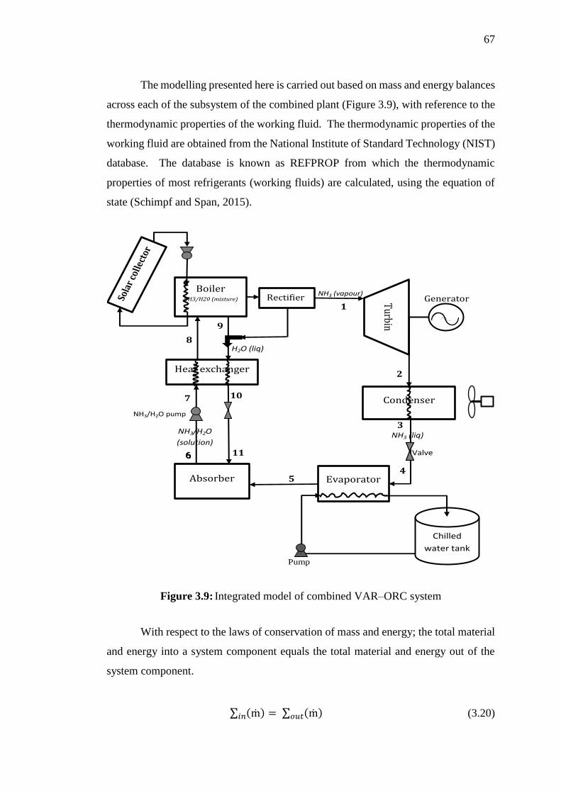
67
The modelling presented here is carried out based on mass and energy balances
across each of the subsystem of the combined plant (Figure 3.9), with reference to the
thermodynamic properties of the working fluid. The thermodynamic properties of the
working fluid are obtained from the National Institute of Standard Technology (NIST)
database. The database is known as REFPROP from which the thermodynamic
properties of most refrigerants (working fluids) are calculated, using the equation of
state (Schimpf and Span, 2015).
Figure 3.9: Integrated model of combined VAR–ORC system
With respect to the laws of conservation of mass and energy; the total material
and energy into a system component equals the total material and energy out of the
system component.
∑ (ṁ)𝑖𝑛 = ∑ (ṁ)𝑜𝑢𝑡 (3.20)
Evaporator
Condenser
Generator Turbin
e
Rectifier
2
1
Heat exchanger
8
9
11
7 10
Absorber
3
4 5
Boiler NH3/H20 (mixture)
Chilled
water tank
NH3/H2O
(solution)
H2O (liq)
NH3 (vapour)
NH3 (liq)
NH3/H2O pump
Valve
Pump

68
∑ (𝜌1𝑉1𝐴1) = ∑ (𝜌2𝑉2𝐴2)𝑜𝑢𝑡𝑖𝑛 (3.21)
Furthermore, rate of change of internal energy (kinetic and potential) within a
system equals net energy transferred by heat, work and mass within the system.
𝑑É𝑠𝑦𝑠𝑡𝑒𝑚
𝑑𝑡= É𝑖𝑛 − É𝑜𝑢𝑡 (3.22)
But at steady state;
𝑑É𝑠𝑦𝑠𝑡𝑒𝑚
𝑑𝑡= 0
Therefore, É𝑖𝑛 = É𝑜𝑢𝑡
Ǭ𝑖𝑛 + Ẃ𝑖𝑛 + ∑ ṁ (ℎ +𝑉2
2+ ᵷ𝑧)𝑖𝑛 = Ǭ𝑜𝑢𝑡 + Ẃ𝑖𝑛 + ∑ ṁ (ℎ +
𝑉2
2+ ᵷ𝑧)𝑜𝑢𝑡 (3.23)
Considering the energy balance with respect to sign convention, that is;
𝐸𝑛𝑒𝑟𝑔𝑦 𝑖𝑛𝑝𝑢𝑡𝑎𝑛𝑑
𝑊𝑜𝑟𝑘 𝑜𝑢𝑡𝑝𝑢𝑡} ⇒ 𝑃𝑜𝑠𝑖𝑡𝑖𝑣𝑒 &
𝐸𝑛𝑒𝑟𝑔𝑦 𝑜𝑢𝑡𝑝𝑢𝑡𝑎𝑛𝑑
𝑊𝑜𝑟𝑘 𝑖𝑛𝑝𝑢𝑡} ⇒ 𝑁𝑒𝑔𝑎𝑡𝑖𝑣𝑒
Ǭ − Ẃ = ∑ ṁ (ℎ +𝑉2
2+ ᵷ𝑧) − ∑ ṁ (ℎ +
𝑉2
2+ ᵷ𝑧)𝑖𝑛𝑜𝑢𝑡 (3.24)
It is also assumed that the changes in potential and kinetic energy are
negligible, therefore;
Ǭ − Ẃ = ṁ(ℎ2 − ℎ1) (3.25)
Meanwhile, for component sizing, the size of each of the components is
expressed in terms of the component heat transfer area (𝐴ℎ𝑡) in m2. This is given as;
69
𝐴ℎ𝑡 =Ǭ
𝑈.∆𝑇𝑙𝑚=
ṁ(ℎ2− ℎ1)
𝑈.∆𝑇𝑙𝑚 (3.26)
Where 𝑈 is the component heat transfer coefficient, ṁ is the fluid mass flow rate,
ℎ2& ℎ1 are the inlet and outlet enthalpies of the fluid across the component, and ∆𝑇𝑙𝑚
is the logarithmic temperature difference between the inlet and outlet fluid.
3.2.2.1 VAR–ORC Combined Plant Components Modelling
The present system is designed to overcome a particular load size. Therefore,
the modelled plant size is equivalent to the load requirement of interest. The modelling
isنdoneنwithنrespectنtoنtheنmassنandنenergyنbalanceنacrossنtheنplant’sنcomponentنparts.نن
To determine the energy and mass balance, each of the plant components is treated as
a separate entity (as represented in Figure 3.10) over which the energy and mass
balances are carried out. The major components of the combined plant include; boiler,
turbine, condenser, evaporator, absorption tank, and solution heat exchanger. Mass
and energy balances have always been the focal point in component modelling of ORC
and sorption cooling systems. Dynamic model for a 30kW LiBr-H2O (single-effect)
absorption chiller was developed by (Marc et al., 2012), considering steady and
transient states based on mass and energy balances of each of the system components,
together with the equations of state and heat transfer. Series of modelling with mass
and energy balances have been carried out by various researchers (Hong et al., 2011;
Borunda. et al., 2016; Pratihar et al., 2010; Sanjay, 2003). To simplify the
mathematical modelling of the combined plant, the following assumptions were made.
1. The plant operates at steady state and the fluids are incompressible.
2. Heat transfer between the system and environment is negligible
3. Expansion through the throttling valve is isentropic (h3 = h4), so zero work
done is assumed across the valve.

70
Figure 3.10: Component energy balance model
Heat is supplied to the boiler from the solar collector via the hot collector fluid
(water) to indirectly heat up and vaporize the refrigerant (NH3) from the working fluid
solution (NH3-H2O). The working fluid is a solution mixture of Ammonia (NH3) and
water (H2O), originally in 35 % and 65 % composition respectively. The total heat
gained by the working fluid in the boiler (𝑄𝑏𝑜𝑖𝑙𝑒𝑟), is modelled as the product of mass
flow, and the enthalpy difference of the working fluid stream between the inlet and
outlet of the boiler (Abed et al., 2013). From the boiler, the superheated vapour
ammonia exits with high pressure to the turbine. The energy balance across the boiler
is given as;
Ǭ𝑏𝑜𝑖𝑙𝑒𝑟 = ṁ1ℎ1 + ṁ9ℎ9 − ṁ8ℎ8 (3.27)
The mass fraction of the working fluid mixture components is expressed in
equation 3.28 as;
ṁ8 = ṁ1 + ṁ9 → ṁ8𝑋8 = ṁ1𝑋1 + ṁ9𝑋9 (3.28)
ṁ8=1−𝑋9
𝑋8−𝑋9ṁ1
ṁ9 =1 − 𝑋8
𝑋8 − 𝑋9ṁ1
The material size of the boiler is determined by considering the heat transfer
area (𝐴𝑏) of the boiler, as expressed in equation 3.29. However, the material type and
properties play a major role in the component sizing.
, , , , ℎ , , ḿ , , , , ℎ , , ḿ

71
𝐴𝑏 =Ǭ𝑏𝑜𝑖𝑙𝑒𝑟
𝑈.∆𝑇𝑙𝑚 (3.29)
Where X represents the NH3 mass fraction in the working fluid, ṁ𝑟, ṁ𝑤, and ṁ𝑠𝑜𝑙 are
the mass flow rates of ammonia, water, and NH3-H2O solution respectively, h is the
enthalpy of the fluids, ∆𝑇𝑙𝑚 is the logarithmic temperature difference between the inlet
and outlet fluids, 𝑈 is the component heat transfer coefficient and a function of the
boiler material type and thermal properties.
The superheated ammonia refrigerant vapour expands through the turbine to
produce useful work, which is converted to electrical power by the turbine generator.
The ammonia vapour pressure exit from the turbine is set to be equal to saturation
pressure at the condenser inlet and the condensation is assumed to be isobaric. That
is;
𝑃2 = 𝑃3(𝑠𝑎𝑡) (3.30)
The gross power output (𝑊𝑡) from the turbine-generator is given as;
𝑊𝑡 = ��𝑟(ℎ1 − ℎ2)𝜂𝑡 (3.31)
Where 𝜂𝑡 = isentropic efficiency of the turbine; usually between 80 and 95 %, (Quoilin
et al., 2013).
However, it should be noted that turbine efficiency values in power generation
systems largely depends on the fuel (heat source) type, and conversion technology
employed.
The NH3 vapour exiting the turbine is cooled and condensed in the condenser,
loosing most of its heat to become saturated liquid. For the modelled plant in this
study, condenser pressure is kept at 10bar and the corresponding (saturated) ammonia
temperature at this point is 25 ℃. Heat removed from the condenser (��𝑐) is given as;

72
��𝑐 = ��𝑟(ℎ2 − ℎ3) (3.32)
Passing through the throttling (expansion) valve, the liquid refrigerant
undergoes a pressure reduction, making its temperature to drastically reduce. The
extremely cold refrigerant flows into the evaporator where it evaporates and exchanges
heat with chilled water in the evaporator. The heat removed from the evaporator (��𝑒𝑣𝑝)
is known as the refrigeration effect (cooling effect) of the cooling system. This is given
as;
��𝑒𝑣𝑝 = 𝑚𝑟 (ℎ5 − ℎ4) (3.33)
ℎ3 = ℎ4 (3.34)
The chilled water flow rate at the evaporator is determined using the heat
transfer relations between the chilled water and the chilled evaporator tube, with
respect to the heat transfer coefficient between them.
ḿ𝑐𝑤 =𝑈𝑐𝐴𝑒𝑣𝑝(∆𝑇𝑒𝑣𝑝)
𝐶𝑝𝑐𝑤(∆𝑇𝑐𝑤) (3.35)
Where ∆𝑇𝑤 & ∆𝑇𝑒𝑣𝑝 are the respective changes in temperatures of the chilled water
and working fluid, 𝐶𝑝𝑐𝑤 is the chilled water heat capacity, and 𝐴𝑒𝑣𝑝 are the area of
the evaporator which can be determined using equation 3.26.
Leaving the evaporator, the refrigerant then exits as saturated vapour, and flows
to the absorption tank where it is absorbed by the low pressure absorbent (H2O) to
again form the solution mixture. From the absorption tank, the solution mixture is
pumped back (through the solution heat exchanger) to the boiler to repeat the cycle.
The energy balance at the absorption tank is given as;
��𝑎𝑏𝑠 = 𝑚5ℎ5 + 𝑚11ℎ11 − 𝑚6ℎ6 (3.36)
73
This is also expressed as;
��𝑎𝑏𝑠 = 𝑚𝑟ℎ5 + 𝑚𝑤ℎ11 − 𝑚𝑠𝑜𝑙ℎ6
The solution heat exchanger (sometimes called pre-heater) is used to maximize
the heat energy recovery process (internal energy recovery) by exchanging heat
between the hot fluid (absorbent) coming from the boiler and the cold high-pressure
working fluid from the absorber. The heat transfer between the two streams is
modelled by considering the energy transfer by the streams across the component at
their different temperatures. The amount of heat exchanged is given as;
��𝐻𝑥 = ḿ7ℎ7 + ḿ9ℎ9 − ḿ8ℎ8 − ḿ10ℎ10 (3.37)
This is also expressed as;
��𝐻𝑥 = ḿ𝑠𝑜𝑙(ℎ7 − ℎ8) + ḿ𝑤(ℎ9 − ℎ10)
Energy is consumed by the solution pump to raise the pressure of working fluid
mixture. The energy consumed by the pump is given as;
��𝑝 =ṁ𝑠𝑜𝑙𝑉7(𝑝7−𝑝6)
𝜂𝑝 (3.38)
Where ṁ𝑠𝑜𝑙 𝑎𝑛𝑑 𝑉 are the mass flow rate and specific volume of H2O-NH3 solution
through the pump, 𝜂𝑝 is the efficiency of the solution pump, 𝑝6 & 𝑝7 are the inlet and
exit pressure through the pump.
Effective solar collector size required for the system activation is determined
using (Bajpai, 2012; Yeh. et al., 2002)relation, expressed as;
𝑄𝑢 = 𝑄𝑖𝑛𝑐 × 𝐴𝑐 (3.39)
74
𝑄𝑏 = 𝑘𝑄𝑢 (3.40)
Where 𝑘 is the efficiency of the solar collector, 𝑄𝑢 is the solar energy (W) absorbed
by the collector, 𝑄𝑖𝑛𝑐 is the available solar heat (per square metre) on the earth (W/m2),
𝐴𝑐 is the effective area of the collector.
3.2.3 Combined Plant–Cooling Load–Piping Systems Integrations
The modelled cooling load (𝑄𝑙𝑜𝑎𝑑) is expressed as the product of the net heat
gained by the soil and a safety factor (𝛾). Safety factor is commonly added to
accommodate possible variation in design values so that the system can optimally cope
with variations in load (Flueckiger et al., 2013) This has been applied by previous
researchers in similar areas of study by adding 10–25 % of the designed values (Liu.
et al., 2014; Sharizal, 2006) depending on the complexity of the design.
𝑄𝑙𝑜𝑎𝑑 = 𝑄𝑠 × 𝛾 (3.41)
The equivalent chiller capacity (𝑄𝑒𝑣𝑝) is expressed as the product of the cooling
load and the area of the soil bed to be cooled.
𝑄𝑒𝑣𝑝 = 𝑄𝑙𝑜𝑎𝑑 × 𝐴𝑠 (3.42)
𝐴𝑠 =𝑄𝑒𝑣𝑝
𝑄𝑙𝑜𝑎𝑑 (3.43)
Relating the chilled water tube cooling capacity (with respect to soil bed area)
with the plant cooling capacity gives the approximate length of the chilled water pipe
(earth tube). With all specifications appropriately selected, the calculated length is
equivalent to the length of the earth tube that is evenly networked through the soil bed
for even temperature distribution within the soil bed.
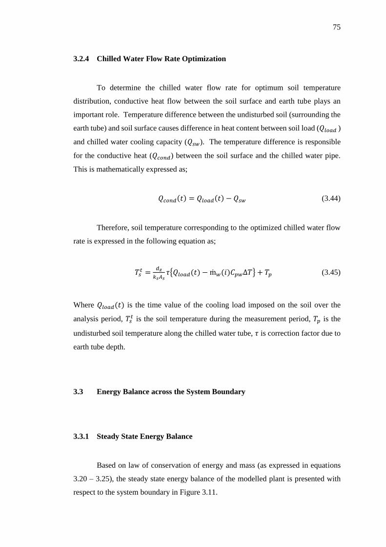
75
3.2.4 Chilled Water Flow Rate Optimization
To determine the chilled water flow rate for optimum soil temperature
distribution, conductive heat flow between the soil surface and earth tube plays an
important role. Temperature difference between the undisturbed soil (surrounding the
earth tube) and soil surface causes difference in heat content between soil load (𝑄𝑙𝑜𝑎𝑑 )
and chilled water cooling capacity (𝑄𝑠𝑤). The temperature difference is responsible
for the conductive heat (𝑄𝑐𝑜𝑛𝑑) between the soil surface and the chilled water pipe.
This is mathematically expressed as;
𝑄𝑐𝑜𝑛𝑑(𝑡) = 𝑄𝑙𝑜𝑎𝑑(𝑡) − 𝑄𝑠𝑤 (3.44)
Therefore, soil temperature corresponding to the optimized chilled water flow
rate is expressed in the following equation as;
𝑇𝑠𝑡 =
𝑑𝑧
𝑘𝑠𝐴𝑠𝜏{𝑄𝑙𝑜𝑎𝑑(𝑡) − ṁ𝑤(𝑖)𝐶𝑝𝑤∆𝑇} + 𝑇𝑝 (3.45)
Where 𝑄𝑙𝑜𝑎𝑑(𝑡) is the time value of the cooling load imposed on the soil over the
analysis period, 𝑇𝑠𝑡 is the soil temperature during the measurement period, 𝑇𝑝 is the
undisturbed soil temperature along the chilled water tube, 𝜏 is correction factor due to
earth tube depth.
3.3 Energy Balance across the System Boundary
3.3.1 Steady State Energy Balance
Based on law of conservation of energy and mass (as expressed in equations
3.20 – 3.25), the steady state energy balance of the modelled plant is presented with
respect to the system boundary in Figure 3.11.
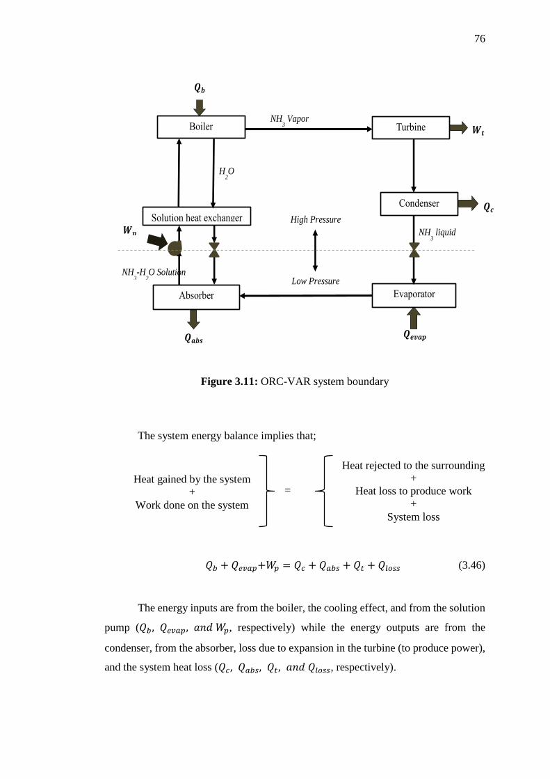
76
Figure 3.11: ORC-VAR system boundary
The system energy balance implies that;
𝑄𝑏 + 𝑄𝑒𝑣𝑎𝑝+𝑊𝑝 = 𝑄𝑐 + 𝑄𝑎𝑏𝑠 + 𝑄𝑡 + 𝑄𝑙𝑜𝑠𝑠 (3.46)
The energy inputs are from the boiler, the cooling effect, and from the solution
pump (𝑄𝑏 , 𝑄𝑒𝑣𝑎𝑝, 𝑎𝑛𝑑 𝑊𝑝, respectively) while the energy outputs are from the
condenser, from the absorber, loss due to expansion in the turbine (to produce power),
and the system heat loss (𝑄𝑐, 𝑄𝑎𝑏𝑠, 𝑄𝑡, 𝑎𝑛𝑑 𝑄𝑙𝑜𝑠𝑠, respectively).
High Pressure
Low Pressure
NH3-H
2O Solution
Boiler Turbine
Condenser
Evaporator Absorber
olutionنheatنexchanger
H2O
NH3 Vapor
NH3 liquid
Heat rejected to the surrounding
+
Heat loss to produce work
+
System loss
Heat gained by the system
+
Work done on the system
=
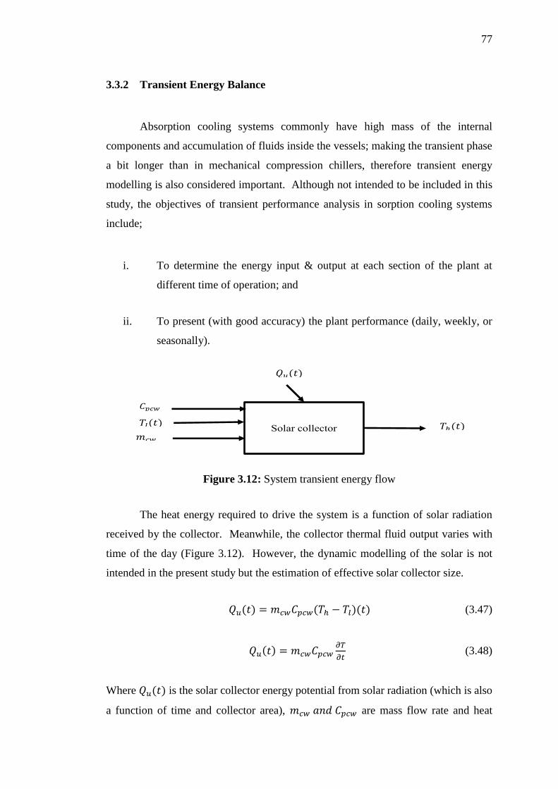
77
3.3.2 Transient Energy Balance
Absorption cooling systems commonly have high mass of the internal
components and accumulation of fluids inside the vessels; making the transient phase
a bit longer than in mechanical compression chillers, therefore transient energy
modelling is also considered important. Although not intended to be included in this
study, the objectives of transient performance analysis in sorption cooling systems
include;
i. To determine the energy input & output at each section of the plant at
different time of operation; and
ii. To present (with good accuracy) the plant performance (daily, weekly, or
seasonally).
Figure 3.12: System transient energy flow
The heat energy required to drive the system is a function of solar radiation
received by the collector. Meanwhile, the collector thermal fluid output varies with
time of the day (Figure 3.12). However, the dynamic modelling of the solar is not
intended in the present study but the estimation of effective solar collector size.
𝑄𝑢(𝑡) = 𝑚𝑐𝑤𝐶𝑝𝑐𝑤(𝑇ℎ − 𝑇𝑙)(𝑡) (3.47)
𝑄𝑢(𝑡) = 𝑚𝑐𝑤𝐶𝑝𝑐𝑤𝜕𝑇
𝜕𝑡 (3.48)
Where 𝑄𝑢(𝑡) is the solar collector energy potential from solar radiation (which is also
a function of time and collector area), 𝑚𝑐𝑤 𝑎𝑛𝑑 𝐶𝑝𝑐𝑤 are mass flow rate and heat
olarنcollector
( )
ℎ( )
( )

78
capacity of the collector thermal fluid, and 𝑇ℎ 𝑎𝑛𝑑 𝑇𝑙 are the respective outlet and inlet
temperatures of the thermal fluid from (and to) the collector.
3.4 Performance Evaluation
Performance analysis of the present system is mainly based on steady state.
The steady state performance evaluation is done to assess the coefficient of
performance and the organic Rankine efficiency of the combined plant. Further
performance analysis is carried out through the parametric analysis and optimization
of the plant by varying the key parameters and studying their effects on the plant
performance. The key parameters of interest in this study are the working fluid
vaporizing temperature and pressure, and the mass fraction of NH3 in the NH3-H2O
working fluid mixture. The parametric analysis is done using RSM of the Design
Expert®. The details are contained in section 3.8.
3.4.1 Power Cycle Efficiency
Power cycle efficiency is defined based on its output of interest. This depends
on whether is it gross power or net power output. The gross power output can be
determined by the turbine shaft power as presented in Equation 3.31. However, the
net power output is affected by the energy consumed by other components (such as the
working fluid pump) during the operation (Schröder et al., 2014). Gross and net power
efficiencies are represented by Equations (3.49) and (3.50), respectively.
𝜂𝑔𝑟𝑜𝑠𝑠 =𝑊𝑡
𝑄𝑖𝑛 (3.49)
𝜂𝑛𝑒𝑡 = {[𝑊𝑡−∑ 𝑊𝑝𝑖]
𝑄𝑖𝑛} (3.50)

79
Where 𝑊𝑝𝑖 represents the power consuming components, 𝑄𝑖𝑛 is the energy required to
vaporize the working fluid.
3.4.2 Cooling Coefficient of Performance
The performance of HVAC system is usually measured in terms of the
Coefficient of Performance (COP), which relates the cooling output to the energy input
for driving the system. This is represented as;
𝐶𝑂𝑃 =Ǭ𝒆𝒗𝒑
Ǭ𝒃𝒐𝒊𝒍𝒆𝒓 (3.51)
3.4.3 Combined Plant Performance
Measuring the performance of power and cooling combined cycle, based on
first law of efficiency by adding the power and refrigeration output then dividing them
by the heat input may result in power cycle exceeding the Carnot efficiency
(Demirkaya et al., 2013); this is justن likeن addingن “orangesن toن apples”ن accordingن toن
(Vijayaraghavan and Goswami, 2003). However, in this study, with cooling as the
primary goal, the performance of the combined plant is expressed as modified COP,
given as;
𝐶𝑂𝑃 = {[ḿ𝑟(ℎ5−ℎ3)]+[(ḿ𝑟(ℎ1−ℎ2)−ḿ𝑠𝑜𝑙𝑉7(𝑃7−𝑃6)]
Ǭ𝑏𝑜𝑖𝑙𝑒𝑟} (3.52)
𝐶𝑂𝑃 =Ǭ𝒆𝒗𝒂𝒑+𝑾𝒏𝒆𝒕
Ǭ𝒃𝒐𝒊𝒍𝒆𝒓 (3.53)
𝑊𝑛𝑒𝑡 = 𝑊𝑡 − ∑ ��𝑝𝑖

80
It is also to be noted that the relative newness of power and refrigeration
systems on a single cycle in the literature (Tamm et al., 2004), resulted in the
modification of the performance calculation expressions.
However, to consider individuals of the two output performances (𝜂𝑂𝑅𝐶
and 𝐶𝑂𝑃𝑐𝑜𝑜𝑙𝑖𝑛𝑔) in relation to the same energy source, their performances can be
represented in equations 3.54 and 3.55, respectively as;
𝜂𝑂𝑅𝐶 =𝑊𝑡
𝑄𝑏−𝑄𝑒𝑣𝑝 (3.54)
𝐶𝑂𝑃𝑐𝑜𝑜𝑙𝑖𝑛𝑔 =𝑄𝑒𝑣𝑝
𝑄𝑏−𝑊𝑡 (3.55)
When the system performance is based on the overall solar energy received by
the collector, equations 3.50 and 3.53 can be modified as;
Ƞ𝑡ℎ𝑒𝑟𝑚𝑎𝑙 = {[𝑊𝑡−∑ 𝑊𝑝𝑖]
𝑄𝑢} (3.56)
𝐶𝑂𝑃𝑡ℎ𝑒𝑟𝑚𝑎𝑙 =Ǭ𝑒𝑣𝑎𝑝+𝑊𝑛𝑒𝑡
Ǭ𝑢 (3.57)
Where ∑ Ǭ𝒑𝒊 indicates the situation where more than one pumps are considered in the
performance measurement, Ǭ𝑢 is the total heat supplied by the collector (through the
thermal fluid).
3.4.4 Soil Cooling Efficiency
The efficiency of soil cooling process considered in this study refers to the
percentage of the soil cooling load that the chilled water is able to overcome. This is
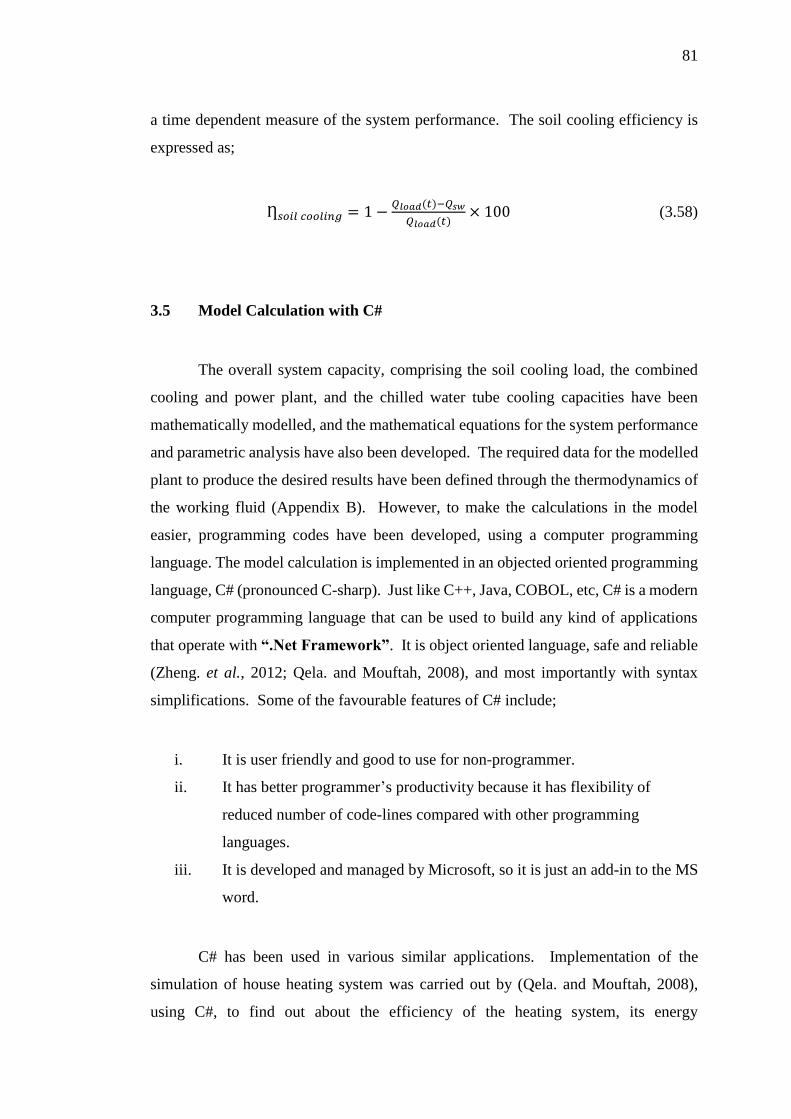
81
a time dependent measure of the system performance. The soil cooling efficiency is
expressed as;
Ƞ𝑠𝑜𝑖𝑙 𝑐𝑜𝑜𝑙𝑖𝑛𝑔 = 1 −𝑄𝑙𝑜𝑎𝑑(𝑡)−𝑄𝑠𝑤
𝑄𝑙𝑜𝑎𝑑(𝑡)× 100 (3.58)
3.5 Model Calculation with C#
The overall system capacity, comprising the soil cooling load, the combined
cooling and power plant, and the chilled water tube cooling capacities have been
mathematically modelled, and the mathematical equations for the system performance
and parametric analysis have also been developed. The required data for the modelled
plant to produce the desired results have been defined through the thermodynamics of
the working fluid (Appendix B). However, to make the calculations in the model
easier, programming codes have been developed, using a computer programming
language. The model calculation is implemented in an objected oriented programming
language, C# (pronounced C-sharp). Just like C++, Java, COBOL, etc, C# is a modern
computer programming language that can be used to build any kind of applications
that operate with “.Net Framework”. It is object oriented language, safe and reliable
(Zheng. et al., 2012; Qela. and Mouftah, 2008), and most importantly with syntax
simplifications. Some of the favourable features of C# include;
i. It is user friendly and good to use for non-programmer.
ii. It has better programmer’s productivity because it has flexibility of
reduced number of code-lines compared with other programming
languages.
iii. It is developed and managed by Microsoft, so it is just an add-in to the MS
word.
C# has been used in various similar applications. Implementation of the
simulation of house heating system was carried out by (Qela. and Mouftah, 2008),
using C#, to find out about the efficiency of the heating system, its energy
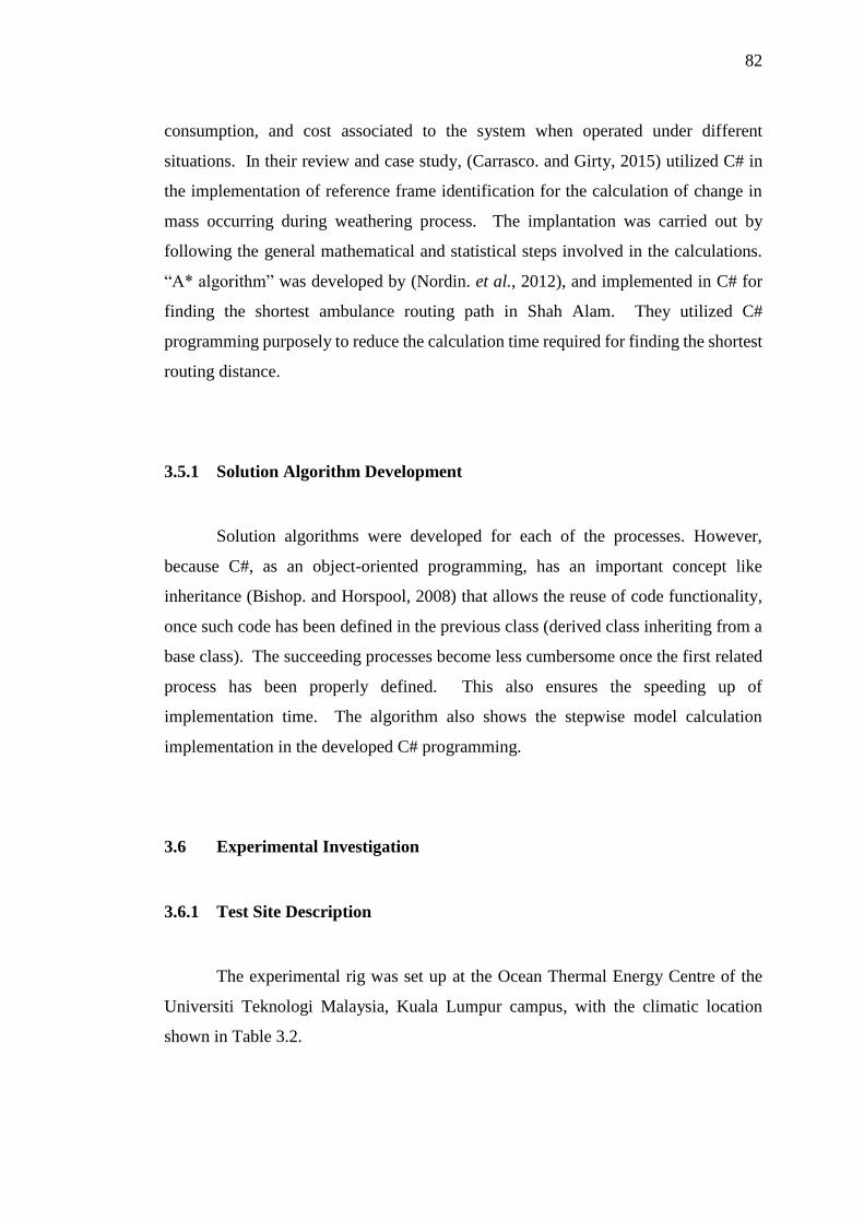
82
consumption, and cost associated to the system when operated under different
situations. In their review and case study, (Carrasco. and Girty, 2015) utilized C# in
the implementation of reference frame identification for the calculation of change in
mass occurring during weathering process. The implantation was carried out by
following the general mathematical and statistical steps involved in the calculations.
“A*نalgorithm” was developed by (Nordin. et al., 2012), and implemented in C# for
finding the shortest ambulance routing path in Shah Alam. They utilized C#
programming purposely to reduce the calculation time required for finding the shortest
routing distance.
3.5.1 Solution Algorithm Development
Solution algorithms were developed for each of the processes. However,
because C#, as an object-oriented programming, has an important concept like
inheritance (Bishop. and Horspool, 2008) that allows the reuse of code functionality,
once such code has been defined in the previous class (derived class inheriting from a
base class). The succeeding processes become less cumbersome once the first related
process has been properly defined. This also ensures the speeding up of
implementation time. The algorithm also shows the stepwise model calculation
implementation in the developed C# programming.
3.6 Experimental Investigation
3.6.1 Test Site Description
The experimental rig was set up at the Ocean Thermal Energy Centre of the
Universiti Teknologi Malaysia, Kuala Lumpur campus, with the climatic location
shown in Table 3.2.

83
Table 3.2: Site reference conditions and project location
Climate data location Kuala Lumpur/Subang
Latitude 3.1 ⁰N
Longitude 101.6 ⁰E
Elevation 22 m
Heating design temperature 16.5 ℃
Cooling design temperature 19.5 ℃
Earth temperature amplitude 7.3 ℃
The day-time solar radiation availability at the test site is usually between
7:00hr and 19:00hr clock time. However, the soil bed was positioned in a place where
it was exposed to about 85 % of the available daytime solar radiation. Thus, it is
expected to exhibit real planting field characteristics.
3.6.2 Experimental Set up
The test rig developed in this study consists of the chilled water production
plant and the soil bed. Thus, the experimental study was conducted in two phases; (i)
chilled water production subsystem and (ii) soil cooling subsystem, as shown in Figure
3.13. Data collected from the set-up include chilled water flow rates and temperatures
from the chiller, the soil bed and the chilled water pipes, using T-type thermocouples.
Each of the subsystems was independently studies and their results were analysed and
compared with those obtained from the mathematical models. The temperatures
recorded during the experimental study were logged to the computer hard disk through
the National instrument data logger.
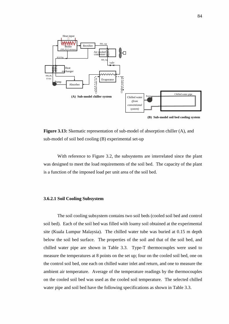
84
Figure 3.13: Skematic representation of sub-model of absorption chiller (A), and
sub-model of soil bed cooling (B) experimental set-up
With reference to Figure 3.2, the subsystems are interrelated since the plant
was designed to meet the load requirements of the soil bed. The capacity of the plant
is a function of the imposed load per unit area of the soil bed.
3.6.2.1 Soil Cooling Subsystem
The soil cooling subsystem contains two soil beds (cooled soil bed and control
soil bed). Each of the soil bed was filled with loamy soil obtained at the experimental
site (Kuala Lumpur Malaysia). The chilled water tube was buried at 0.15 m depth
below the soil bed surface. The properties of the soil and that of the soil bed, and
chilled water pipe are shown in Table 3.3. Type-T thermocouples were used to
measure the temperatures at 8 points on the set up; four on the cooled soil bed, one on
the control soil bed, one each on chilled water inlet and return, and one to measure the
ambient air temperature. Average of the temperature readings by the thermocouples
on the cooled soil bed was used as the cooled soil temperature. The selected chilled
water pipe and soil bed have the following specifications as shown in Table 3.3.
Boiler(NH3/H2O mixture)
Heat input
NH3 liq
Evaporator
Absorber
Rectifier
NH3/H2
O mix
NH3 vap
H2O liq
valve
Pump
Heat
exchanger
Air cooled condenser
Chil
led w
ater
out
Chil
led w
ater
in
(A) Sub-model chiller system Chilled water
(from
conventional
system)
PumpChilled water pipe
(B) Sub-model soil bed cooling system

85
Table 3.3: Soil bed and chilled water pipe specifications
Soil bed container Soil Chilled water pipe
Material
Top
Surface
area
Type Thermal
cond. pH Material Length OD Thickness
Thermal
cond.
Polystyrene
box
0.25
m2 Loamy
1.5
W/m-K
4.85-
5.0 HDPE 1.0 m 0.02m 0.0025m
0.42W/m-
K
High-density polyethylene pipe (HDPE) of 1.0 m length was evenly networked
through the soil bed for the temperature distribution. Chilled water was then pumped
through the buried chilled water pipe to cool the dimensioned soil bed as shown in
Figure 3.14.
Figure 3.14: Experimental soil bed and piping configuration
3.6.2.2 Chilled Water Production Subsystem
The experimental investigation of the chilled water production subsystem had
been done through the study of a mini absorption cooling unit (in Figure 3.15), taking
0.2
5 m
0.1
0 m
0.10 m
0.1
0 m
0.1
5 m
0.2
5 m

86
its operational parameters at steady state to determine its performance characteristics.
The chiller was manufactured by Shandong XINGKE intelligent technology company
limited. It is a thermally activated system, operating on ammonia-water mixture with
0.35/0.65 of NH3/H2O mass fraction, and suitable for chilling a 0.04 m3 space volume
(40 litre) capacity. Table 3.4 gives the basic specification of the chiller, while other
operating details taken during the experimental study are presented in Chapter 4.
Table 3.4: Experimental chiller’sنdesignنspecification
Model Cooling
capacity
Boiler
Pressure
NH3/H2O Mass
Fraction
Total effective
cooling volume
XC-40 50 W 16 bar 0.35/0.65 40 litre
Prior to the experimental study, sections of the evaporator, solution heat
exchanger, and boiler pipes were insulated against the ambient environment to reduce
the interference and losses to as low as possible. The condenser and absorber are air-
cooled and were allowed to be fully exposed to the ambient air; the air-cooling of the
components was aided by a mini fan with 2.5 W capacity. The activation of the chiller
was achieved through an electric heater, and energy delivered by the heater was
quantified in terms of the collector deliverable energy. Chiller’sنrequiredنenergyنwasن
regulated through its thermostat. T-Type thermocouples were used to measure the
operating temperatures and details of the data points are shown in Table 3.5.

87
Figure 3.15: Experimental absorption refrigeration system
3.6.3 Data Collection Methods
The overall set up contained 14 numbers of data collection points; five point
on the chiller, eight on the soil beds and one for the ambient air temperature. Chiller’sن
operating temperatures at the boiler, condenser, evaporator, absorber and solution heat
exchanger were measure via the T-type thermocouples as shown in Figure 3.16).
Condenser
Evaporator
Absorber
Heat exchanger
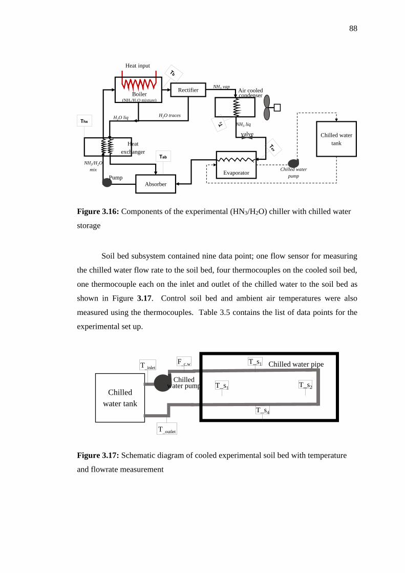
88
Figure 3.16: Components of the experimental (HN3/H2O) chiller with chilled water
storage
Soil bed subsystem contained nine data point; one flow sensor for measuring
the chilled water flow rate to the soil bed, four thermocouples on the cooled soil bed,
one thermocouple each on the inlet and outlet of the chilled water to the soil bed as
shown in Figure 3.17. Control soil bed and ambient air temperatures were also
measured using the thermocouples. Table 3.5 contains the list of data points for the
experimental set up.
Figure 3.17: Schematic diagram of cooled experimental soil bed with temperature
and flowrate measurement
Air cooled condenser
NH3 liq
Evaporator
Absorber
Rectifier
Chilled water
tank
NH3/H2O
mix
NH3 vap
H2O liq
valve
Chilled water
pumpPump
Heat input
Heat
exchanger
Boiler(NH3/H2O mixture)
Thx
Tab
H2O traces
Chilled
water tank
Chilled water pump
Chilled water pipeT_inlet
T_s1F_c.w
T_s4
T_s1T_s2
T_outlet

89
Table 3.5: Instrumentation for the experimental data collection
Data Point Data
Label Medium Measuring Tool
Capacity
Range
Temperature
Cooled Soil bed
T_s 1
T_s 2
T_s3
T_s4
Soil
T – Type Thermocouple
-250 to
+400
Control Soil bed T_control soil
Ambient air (for
soil cooling &
chiller)
T_air Air
Soil bed Chilled
Water Inlet T_inlet
Water Soil bed Chilled
Water outlet T_out
Boiler Exit
Temperature Tb
NH3 Condenser Exit
Temperature Tc
Evaporator
Temperature Tev
Absorber
Temperature Tab
NH3-
H2O Solution Heat
Exchanger Thx
Flow Rates
Chilled water-
to-Soil bed F_c.w H2O
Flow control LCD display
Water sensor
0.01 to
9999 lit/m
National Instrument (NI) data logger was used for the experimental data
acquisition. This required the installation, configuration, and calibration of the test
panel and data measuring tools. Prior to data reading, acquisition and logging, the NI
data logger was installed together with the LabVIEW. This helps in the online
visualization of the acquired data during the experimental campaign. Other data
collection details are contained in Appendix D.

90
3.6.4 Experimental Methods
The experimental rig consists of; (i) the soil cooling subsystem, and (ii) the
chilled water production subsystem.
The chilled water tube was buried in the soil at a depth of 150 mm below the
soil bed surface. The tubes were at 200 mm apart, and 100 mm from the wall of the
soil bed. To achieve the desired soil temperature (18 ℃±2) on the soil bed, four sets
of chilled water flow rate were used and their cooling effects on the soil were observed
at different prevailing weather conditions during the day for the chilled water
temperature between 3 ℃ and 10 ℃. The soil cooling experiment took place between
6:00am to 10:00pm (clock time) within which solar radiation was available. This is
done to observe the effect of chilled water temperature and its flow rates in the presence
and absence of solar radiation heat.
The chilled water production rate was determined by the cooling rate of the
chiller’s evaporator. The chiller unit runs on known operating pressure and working
fluid mass fraction. However, the mass flow rates of the working fluids were
determined, based on its capacity, and operating temperatures and pressures. Working
fluids temperatures at each of the system components were measured from external
surface of the pipes with T-type thermocouples. The true values were however
calculated using Gorman equation (Gorman et al., 2013);
𝑇𝑓𝑙𝑢𝑖𝑑 − 𝑇𝑚𝑒𝑎𝑠𝑢𝑟𝑒𝑑 = (𝑇𝑚𝑒𝑎𝑠𝑢𝑟𝑒𝑑 − 𝑇𝑎𝑚𝑏−𝑎𝑖𝑟) [1−𝜃𝑐𝑟𝑖𝑡
𝜃𝑐𝑟𝑖𝑡] (3.59)
Where; 𝑇𝑚𝑒𝑎𝑠𝑢𝑟𝑒𝑑, 𝑇𝑎𝑖𝑟 and 𝑇𝑓𝑙𝑢𝑖𝑑 are measured temperature, air temperature, and the
actual temperature of the fluid respectively, 𝜃𝑐𝑟𝑖𝑡 is a dimensionless parameter relating
the temperature in x,y,z directions.
The Coefficient of Performance of absorption refrigeration, based on
temperature, has been developed by (Stanish and Perlmutter, 1981), and modified and

91
used for absorption chiller performance verifications by (Kaushik et al., 1983; Mazouz
et al., 2014). However, the theoretically achievable COP based on the ideal cycle
operating on NH3-H2O was reported to be 1.5 (Mazouz et al., 2014) from which only
around 0.5 is actually achievable in the reality (El May et al 2011) from the commercial
absorption chiller cycles.
Further modifications have been made to (Stanish and Perlmutter, 1981)
equation by (Gordon and Ng, 1995) to include the cooling capacity of the chiller in the
analysis of the COP. The modified form of the (Gordon and Ng, 1995) equation
(equation 3.60) is used in this study to analyse the COP of the studied chiller.
1
𝐶𝑂𝑃𝑐𝑜𝑜𝑙𝑖𝑛𝑔= [
𝑇𝑐𝑜𝑛𝑑−𝑇𝑒𝑣𝑝
𝑇𝑒𝑣𝑝] [
𝑇𝑏𝑜𝑖𝑙𝑒𝑟
𝑇𝑏𝑜𝑖𝑙𝑒𝑟−𝑇𝑎𝑏𝑠] + [
1
𝑄𝑒𝑣𝑝] [
𝑇𝑏𝑜𝑖𝑙𝑒𝑟
𝑇𝑏𝑜𝑖𝑙𝑒𝑟−𝑇𝑐𝑜𝑛𝑑] × 𝑄𝑙𝑜𝑠𝑠 (3.60)
Where; 𝑄𝑙𝑜𝑠𝑠 is the system loss (due to the irreversibility) from the components of the
chiller.
𝑄𝑙𝑜𝑠𝑠 = [𝑞𝑐𝑜𝑛𝑑𝑙𝑜𝑠𝑠 + 𝑞𝑎𝑏𝑠
𝑙𝑜𝑠𝑠] − [𝑇𝑐𝑜𝑛𝑑
𝑇𝑒𝑣𝑝× 𝑞𝑒𝑣𝑝
𝑙𝑜𝑠𝑠] − [𝑇𝑐𝑜𝑛𝑑
𝑇𝑏𝑜𝑖𝑙𝑒𝑟× 𝑞𝑏𝑜𝑖𝑙𝑒𝑟
𝑙𝑜𝑠𝑠 ] (3.61)
3.6.5 Modified Cooling and Power System
Upon the exhaustive study of the mini absorption cooling unit, its operational
parameters at steady state were taken to determine its performance characteristics, and
its adaptability with an organic Rankine turbine was investigated. The adaptability is
howeverنaنsimulatedنbased,نreferredنtoنasن“modifiedنcoolingنandنpowerنplant”. The
analysis of the modified plant was carried out based on the operational characteristics
of the experimental absorption chiller unit.
It was reported by (Rice, 1965) that nearly all the pressure drops due to
expansion in ORC turbine occurs in the nozzle. This is caused by reduction in the
nozzle diameter that increases the fluid speed. Therefore the predicted pressure drop

92
could be used to determine the equivalent nozzle diameter for the selected turbine. If
the working fluid pressure differential along the turbine is known, the properties along
this region are used to determine the gross power produced by the turbine; taking the
possible losses into consideration. In the (Rice, 1965) experimental studies on similar
system, the flow of working fluid through the turbine nozzle is considered choked and
nearly all the pressure drop in the turbine occurs at the nozzle with only a negligible
expansion occurring along the rotor. Experimental analysis of Tesla turbine by
(Romanin, 2012) also revealed that at the inlet temperature of similar choked system,
the pressure ratio across the nozzle should be at critical pressure ratio. However,
irrespective of the outlet (downstream) flow condition, the mass flow rate of chocked
flow is constant (Park. et al., 2001). With reference to Figure 3.10, this is simply
expressed in equation as;
𝑃2
𝑃1≈
𝑃𝑛.𝑡
𝑃1 (3.61)
Where 𝑃1, 𝑃2, and 𝑃𝑛.𝑡 are the turbine inlet, outlet, and throat pressures, respectively.
However, (Munson. et al., 2009), cited by (Romanin, 2012) gave the critical
pressure ratio of turbine with air as working fluid at 350K to be about 0.53. It should
be noted that the experimental machines in the references used different working fluids
and this may not make the results obtained from this study to be a perfect match with
them. However, this gives an approximate ranges of expected performance from the
chosen turbine and also displays how the turbine performance correlates with the its
geometries and operational parameters (Rice, 1965).
This approach is also helpful because the experimental rig in this study is
miniature in size, making it a bit difficult to secure a suitable turbine size. Moreover,
it is reported that the knowledge of the turbine nozzle geometries and/or fluid
characteristic can help in predicting the power and efficiency deliverable from the
turbine (Neckel and Godinho, 2015). The conceptual turbine nozzle diameter is
determined using Bernoulli equation;

93
𝑃1 + 12⁄ 𝜌𝑉1
2 + 𝜌𝑔ℎ1 = 𝑃2 + 12⁄ 𝜌𝑉2
2 + 𝜌𝑔ℎ2 (3.63)
The passage of the working fluid through the nozzle (with reduced diameter)
resultsن inنoccurrenceنofن“choke” along the flow in the tube, leading to decrease in
pressure of the fluid, and increase in its velocity but with no effect on the mass flow
rate at the downstream (Javidmand and Hoffmann, 2016). However, height is not
considered in this study, which is a closed system. Therefore, the equation 3.63 is
rewritten in relation to the present study as;
𝑃𝑖 +1
2𝜌𝑣𝑖
2 = 𝑃𝑜 +1
2𝜌𝑣0
2 (3.64)
Based on the continuity equation, the fluid mass flow (ḿ𝑟) through the turbine
nozzle is constant and determined as;
ḿ𝑟 = 𝜌𝑟𝐴𝑖𝑣𝑖 = 𝜌𝑟𝐴𝑜𝑣0 (3.65)
Substituting the fluid velocity term in equation 3.63 with(ḿ𝑟
𝜌𝐴), the pressure
change of the working fluid in the nozzle is expressed as;
∆𝑃 =1
2(
ḿ𝑟2
𝜌) [
1
𝐴𝑜2 −
1
𝐴𝑖2] (3.66)
Where 𝜌 𝑎𝑛𝑑 𝐴 are the density of the working fluid, and the cross sectional area of the
nozzle, and can be written as;
∆𝑃 =1
2(
𝑚𝑟2
𝜌) [
11
4(𝜋𝑑𝑜
2)−
11
4(𝜋𝑑𝑖
2)] (3.67)
The thermodynamic properties of the working fluid together with the prevailing
operating conditions were analysed to assess the performance of the turbine for its
applicability in this system of combined cooling and power. The expansion of the

94
working fluid through the nozzle (due to diameter reduction) leads to the transfer of
the working fluid momentum into kinetic energy that causes the rotation of the turbine
discs.
Changes in working fluid properties at the nozzle diameter were observed and
used for calculating the equivalent work done across the section, using equation 3.68
which is analogous to the one-dimensional model by (Song et al., 2017) in equation
3.69 for calculating the turbine output power.
𝑊𝑡 = ḿ𝑟(ℎ𝑖 − ℎ𝑜)𝜂𝑡 (3.68)
𝑊𝑡 = ḿ𝑟(𝑣𝑖𝑈𝑖 − 𝑣𝑜𝑈𝑜) (3.69)
Experimental analysis of Tesla turbine was first conducted by (Rice, 1965) and
it was concluded that the turbine efficiency could be improved up to 90 %. Similarly,
the experimental studies by (Ho-Yan, 2011) on Tesla turbine indicated the possibility
of more than 70 % efficiency. The studies conducted by (Deam et al., 2008) on mini
scale Tesla turbines (with sub centimetre diameter) using viscous working fluid
showed that the efficiency can be up to 40 % while the experimental and computational
analyses of Tesla turbines by (Hoya and Guha, 2009) gave efficiency of 25 %.
However, the turbine nozzle designed by same authors was able to improve the
efficiency beyond 25 %. These series of previous research give an excellent basis for
the verification of the present micro-scale turbine to be suitable in this application.
3.7 Model Validation
To establish the reliability of the method used in research and the consistency
of the results obtained from such method, model validation is utmost required and this
has always been considered the final stage in the application of system analysis
(Sakellari, 2005). The model developed by (Ayompe. et al., 2011) on forced
circulation of solar water heating using evacuated tube and flat plate collectors was

95
validated with experimental data under different operating and weather conditions.
Cooling and heating performance models for embedded pipe and ground source heat
exchangers have been developed by (Safa. et al., 2015; Liu et al., 2016) and were both
validated with experimental data to access possible improvement in the system. The
model validation path in this study is shown in Figure 3.18. This is followed by
parametric analysis and optimization of the modelled system performance with respect
to variations in its key operating parameters.
Figure 3.18: Validation path
3.8 Models Parametric Analysis
The performance of thermodynamic systems (such as thermally activated
cooling and power) is largely dependent on the suitable selection of the operational
parameters. Therefore, assessment of the system performance and its optimization
Start
Operational
Parameters
Experimental
Setup
Developed
Model
Measured
Results Modeled
Results
Evaluation
(Comparison)
End
System Description

96
have always been based on investigation of the influence of each of the system’s key
parameters (Lee and Strand, 2008). The effects of air flow rates, pipe dimension
(length, diameter, and thickness) on heat transfer between the ground buried pipes
were investigated by (Moncef and Kreider, 1996; Ahmed et al., 2016) through the
parametric analysis.
In this study, the modelled and experimental soil cooling had majorly taken
into consideration, the effects of chilled water flow rates. The chilled water
temperature had been kept within a range, while the climatic effect (in the form of
ambient air temperature due to solar radiation) could not be controlled. Parametric
study is further conducted on the cooling process using the response surface
methodology (RSM) of the Design Expert® software version 10, for further analysis.
Response surface methodology (RSM) comprises of mathematical and statistical
analysis tools, suitable for defining effects of independent parameters (either
separately or in combination) on the output (Hariharan et al., 2013). With RSM,
performance evaluation can be made at intermediate levels that might not have been
experimentally studied (Hariharan et al., 2013; Rout et al., 2014). Central composite
design (Custom) of the RSM was used in this study with 20, and 23 number of (totally
randomized) runs to analyse the parameters for the soil cooling and combined plant
models, respectively. The key parameters (regarded as factors) and their effects
(regarded responses), as well as their types and levels are shown in Table 3.6. Further
results of the parametric analysis are presented in Chapter 4.

97
Table 3.6: Factors and responses for system parametric analysis
Process Factors Responses
Name Type Level Range
Soil
Cooling
Ambient air
Temperature Continuous N/A (25–35) ℃
Soil Temp
(T_s)
Chilled water
Temperature Continuous N/A (1.5–8.5) ℃
Flow rates Discrete 4 (0.24–0.6)
kg/min
Combined
Plant
Boiler’sن
Temperature Discrete 8 (65–65) ℃
W_t, W_sp,
Q_loss,
COP_cooling,
ORC_eff,
COP_overall,
Boiler’sنpressure Discrete 4 (21–21) bar
Working fluid
mass fraction Continuous N/A 0.3–0.7
The analysis of variance (ANOVA) was performed to assess the interaction
between the factors and responses of the system. Probability (p-value) and Fisher
variation ratio (F-value) were used to determine the significance of the models, and
specifically, a p-value not more than 0.05 is desirable (Rout et al., 2014; Puri et al.,
2002; Hariharan et al., 2013; Gontard et al., 1992), which indicates 95 % confidence
interval. The qualities of fit of the models (F-values and P-values) were however
checked to determine the model significance. Furthermore, the diagnostic plots of the
models interaction were observed to check if the model responses are within the set
boundary; for this, LAMBDA values within the required minimum and maximum
values are desirable. Additional results of the parametric analysis are contained in
Appendix G.
3.8.1 Soil Cooling Analysis
In the soil cooling experiments (as described in the previous sections), the
effects of selected chilled water flow rates over a range of temperatures were studied.
However, ambient air temperature also plays an important role on soil temperature and

98
affects the performance of chilled water application on the cooled soil temperature.
The effects of variation in values of these chilled water flow rates and temperature, and
that of ambient air temperature are further studied on the performance of the chilled
water application for soil cooling. Using the developed model, the effects of variation
in experimental values of the chilled water temperature and flow rates, as well as the
temperature of the ambient air were examined on the soil temperature. This was done
to determine the most relevant factor that affects the cooled soil temperature and the
level of significance of the effect.
3.8.2 Combined Plant Analysis
Parametric analysis plays an important role in the performance enhancement
of Rankine cycle and sorption cooling systems and has been applied for such in various
studies (Tamm, 2003; Tamm et al., 2004; Padilla et al., 2010; Yang et al., 2017; Sukri
et al., 2016). The performance investigation through the parametric analysis in this
study is presented in the following sections (3.8.2.1 – 3.8.2.3)نusingن theن“Responseن
Surface Methodology”نofنtheنDesignنExpertنthatنallowsنsimultaneousنanalysisنofنmore
than one factors and responses; unlike the conventional “One-Factor-At-Time”
(OFAT).
3.8.2.1 Working Fluid Boiling Temperature
The performance of a thermally activated system is highly dependent on the
temperature available for its activation. This influences the performance of the
sorption cooling system, the Rankine power cycle as well as the combined cycle
systems. In this study, investigation is carried out on the sensitivity of the system to
change in working fluid boiling temperature from the design value.

99
3.8.2.2 Turbine Inlet Pressure
The effect of pressure differential due to expansion through the turbine is
normally felt on the Rankine power efficiency. However, since the plant in this study
is a combined cycle of Rankine and absorption cooling, the resultant effect of system
sensitivity to turbine inlet pressure is investigated on the combined cycle.
3.8.2.3 Working Fluid Mass Fraction
The cycle makes use of multicomponent working fluid (refrigerant and
absorbent) for which the composition is very sensitive to its thermodynamic properties
at each stage of the cycle, and ultimately on the general performance of both the power
and the cooling systems. The study investigated the sensitivity of the combined cycle
performance with respect to a range of NH3 proportion in NH3-H2O mixture.
3.9 Project Analysis with RETScreen®
Decision making on Renewable Energy Technologies (RETs) remains critical
to implementation of clean energy projects because, the prove that a similar technology
is cost-effective and reliable in some locations may not be enough to establish same in
other locations (Ackom, 2005). Although not intended to be a detailed engineering
design tool (Ackom, 2005), RETScreen software is purposely developed for pre-
feasibility and feasibility studies of RETs projects at the initial stage. The software is
a stepwise program (as shown in Figure 3.19) and contains data tools that run on
Microsoft Excel spread-sheet with various inbuilt project models that include; (i)
Energy efficiency measures, (ii) Power, (iii) Power-multiple technologies, (iv)
Heating, (v) Cooling, (vi) Combined heating and power, (vii) Combined cooling and
power, (viii) Combined heating and cooling, (ix) Combined cooling, heating and
power, and (x) User defined models.
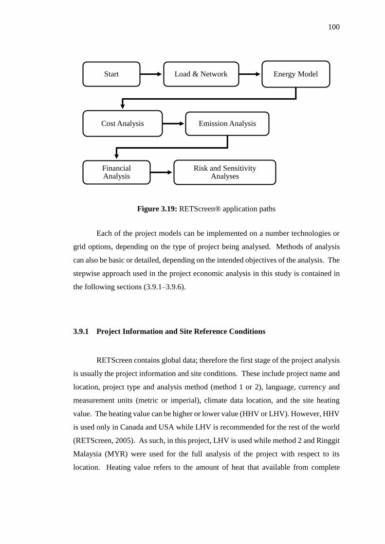
100
Figure 3.19: RETScreen® application paths
Each of the project models can be implemented on a number technologies or
grid options, depending on the type of project being analysed. Methods of analysis
can also be basic or detailed, depending on the intended objectives of the analysis. The
stepwise approach used in the project economic analysis in this study is contained in
the following sections (3.9.1–3.9.6).
3.9.1 Project Information and Site Reference Conditions
RETScreen contains global data; therefore the first stage of the project analysis
is usually the project information and site conditions. These include project name and
location, project type and analysis method (method 1 or 2), language, currency and
measurement units (metric or imperial), climate data location, and the site heating
value. The heating value can be higher or lower value (HHV or LHV). However, HHV
is used only in Canada and USA while LHV is recommended for the rest of the world
(RETScreen, 2005). As such, in this project, LHV is used while method 2 and Ringgit
Malaysia (MYR) were used for the full analysis of the project with respect to its
location. Heating value refers to the amount of heat that available from complete
Start Load & Network Energy Model
Cost Analysis Emission Analysis
Financial Analysis
Risk and Sensitivity Analyses

101
combustion of fuel; measured as a unit of energy per unit mass (kJ/kg) or volume of
substance (J/mol).
3.9.2 Base Case Load and Network
The load and network section of the analysis looks into the base case cooling
load (base load and peak load) with respect to the floor/soil bed area (m2) to be cooled
as well as fuel consumption (kWh) and rate (RM/kWh). Also considered at this stage
is the power source and technology required for the power generation as well as the
costs of generating the power to be used for the cooling system under the base case.
The proposed system characteristics were also analysed with further details in
Appendices H.
3.9.3 Energy Model
Thisنisنtheنpartنofنtheنanalysisنcontainingنtheن‘ olarنResource and Heating Load
calculation worksheets that is used for calculating the passive solar design annual
energy production with respect to system specifications, and site location and
conditions.
3.9.4 Cost Analysis
The cost contents of the project economic analysis include the initial costs and
annual costs. The initial cost which is also referred to as capital cost (Abdullah and
Hieng, 2010) or total investment cost takes the major share of the total project cost in
this study. It usually comprises of the costs associated with; project feasibility study,
project development, engineering design, procurement of components and spare parts,
and miscellaneous expenses.

102
On the other hand, the annual cost (annual operating cost) refers to the cost
incurred during the service life of the project. This is expressed by (Abdullah and
Hieng, 2010) as;
𝐶𝑜𝑝 = 𝐶𝑓𝑐 + 𝐶𝑚 (3.70)
Where 𝐶𝑜𝑝 is the annual operating cost, 𝐶𝑓𝑐 is the annual fuel cost and 𝐶𝑚 is the annual
maintenance cost of the project.
In this project, the initial cost is based on the quotation obtained from the
supplier. Meanwhile, procurement of parts and engineering design form the major
parts of the initial cost. This is because of the project is a mini type and falls under
those for which feasibility and development costs can be ignored (RETScreen, 2005).
It is recommended that the feasibility should be between 1 % and 5 % of the total
project cost, and for smaller project, the proponent can go directly to engineering stage
as the development and feasibility costs may not be justified due to the size of the
project. Further details of the project cost are shown in Appendix H.
3.9.5 Emission Analysis
International Energy Agency (IEA) statistics showed that about 42 % of the
total global CO2 emission came from burning of fossil fuels purposely for electricity
and heat supply in the year 2011 (Mansouri Majoumerd and Assadi, 2014).
Meanwhile, one of the objectives of the application of RETs systems is to reduce the
carbon footprints in the atmosphere for safe and healthy environment (Leavell, 2010;
Kalkan et al., 2012; Khan and Pervaiz, 2013). Therefore, in dealing with economic
analysis of RETs systems, the impact on environment is always considered and
compared with a base case that uses non-renewable energy systems (Smith et al.,
2013). In this study, the emission analysis is done based on the fuel type used to power
the cooling system and on the GHG emission reduction from the system
implementation.
103
The model gives the emission reduction summary for both power and cooling
systems of the proposed case in tons of carbon dioxide (tCO2) equivalence and net
annual GHG emission is calculated and quantified in terms of number of barrels of
crude oil (not consumed) for implementing this project instead of the base case. More
details are contained in appendices H.
3.9.6 Financial Analysis
This section of the economic analysis is concerned with the selection of
operating financial parameters that allow the calculation of; project cost and savings,
annual income, financial viability, yearly cash flows, and cumulative cash flows graph.
The financial parameters include but not limited to fuel/electricity cost escalation and
general inflation rates, with common values between 2 and 3 % (RETScreen, 2005),
discount rate (that is used to calculate annual-life-cost savings), incentives and grants,
debt ratio (0–90 %), interest rate on debt (%), term of debt (year), debt payment plan,
effective income tax (%), depreciation method, rate (%) and period (year), and the
proposed project life that depends on the prevailing circumstances.
In this study, the project cost and savings contained in the financial analysis
worksheets were calculated based on inputs from the cost analysis which are mainly
the engineering design, procurement of parts and miscellaneous expenses. Annual
income basically contains income accrued from electricity cost savings and export,
sales of proceeds from the cooled soil, and GHG reduction resulting from using this
RETs applications. Financial feasibility of the project focuses on the pre and after tax
on equity and assets, simple and equity payback, annual life cycle saving, and benefit-
to-cost (B-C) ratio, that also gives indication of the project viability. Yearly and
cumulative cash flows are net cash flows (pre & after tax) over the life of the project
in tabular and graphical representation respectively.

104
3.10 Summary
In this chapter, models had been developed for; (1) the calculation of soil
cooling load, (2) the component model and sizing of the combined cooling and power
plant to optimally deliver the cooling required to overcome the load of a particular size
of the soil bed, and (3) the piping requirement and chilled water flow rates. Computer
programming codes (in C#) had been developed for implementation of the model
calculations. Based on the developed models, an experimental rig were developed and
tested to validate the modelled systems. The parametric analyses of the modelled plant
have been carried out for its performance assessment, using Design Expert®.
After the technical analysis of the modelled system, the economic analysis had
been carried out with RETScreen® Software to assess the financial viability of the
developed system for cooling application. This analysis is normally done in
comparison of any proposed model with a base case. The results of both the technical
and economic analysis are presented in the following chapter.
105
CHAPTER 4
4 RESULTS AND DISCUSSION
4.1 Introduction
As highlighted in the previous chapter, the modelled system is made up of soil
cooling subsystem and combined plant (for power and cooling) subsystem. The
modelling of the plant was preceded by soil cooling load model. The soil cooling
model was used to predict the cooling load, which in turn helped in estimating the
optimum plant size required to offset the predicted loads (Sharizal, 2006). Based on
the model specifications, test rigs, comprising of laboratory-scale soil bed, and an
absorption chiller of equivalent capacity were used for the experimental verification of
the model. The chilled water application for soil cooling during daytime and the
cooling production from the chiller were experimentally studied and their
performances were analysed. Results from the experimental rigs were then compared
with those obtained from the mathematical analysis for the validation of the developed
models. Parametric analyses were carried out on the soil cooling and the combined
plantنusingن“Responseن urfaceنMethodologyن(RSM)”نofنtheنDesignنofنExpert®.
The economic analyses of system, based on the balance of all expenses and
income from the developed system have been carried out not only to assess the
feasibility of the system, but also its financial viability and emission reductions: this is
basically done in comparison with a base case (Sabetia. and Boyaghchi, 2016;
Stevanovic, 2016; Boyano et al., 2013). Thus; the base case that in this study is
electricity powered system of the same capacity for the same amount of load, and
operated under the same condition for the same length of time.
106
4.2 Modelled Systems Characteristics
With details in section 3.6.2.1 of Chapter 3, the modelled soil cooling load has
been analysed with reference to the solar insolation for Kuala Lumpur–Subang Station,
obtained from the National Aeronautic and Space Administration (NASA); as
contained in the Appendix A. Other parameter values involved in the analytical
models calculations were obtained from published literatures.
Sorption cooling systems are usually rated based on the nominal cooling
capacity (Tozer et al., 2005; Wang et al., 2011; Yin et al., 2013; Thongtip and
Aphornratana, 2017), also referred to as refrigeration capacity. This is used in most
cases to determine the working fluid mass flow rate of the system with known
operating temperatures and pressures. The present cooling subsystem consists of a 50
W rated cooling capacity vapour absorption chilling plant. In modelling the plant, the
thermodynamic properties of the working fluids (from REFPROP) were made use of.
The working fluid is Ammonia-water mixture with 0.35/0.65 (NH3/H2O) initial
composition. Soil cooling analysis was based on the effects of chilled water flow rates
and temperatures on the soil during the daytime, using four sets of chilled water flow
rates.
4.3 Analytical Results
In modelling of combined power and cooling plant, using the mixture of
NH3/H2O working fluid, it is suggested by (Xu. et al., 2000; Lu. and Goswami, 2002)
that; for cycle performance, there exist some optimum operating conditions. In this
study of the combined cooling and power cycle, optimum conditions were selected
based on similar cycles (published in the literature) for the combined cycle and/or
individuals of the ORC and VAR cycles. Based on the selected conditions, the
thermodynamic properties of the working fluid at the major stages of the modelled
cycle plant were used in the model calculations. Modelling of the combined plant was
carried out with respect to operating pressures, temperatures, and working fluid
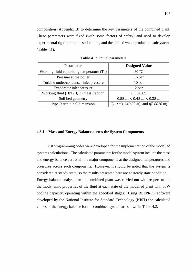
107
composition (Appendix B) to determine the key parameters of the combined plant.
These parameters were fixed (with some factors of safety) and used to develop
experimental rig for both the soil cooling and the chilled water production subsystems
(Table 4.1).
Table 4.1: Initial parameters
Parameter Designed Value
Working fluid vaporizing temperature (T-r) 80 ℃
Pressure at the boiler 16 bar
Turbine outlet/condenser inlet pressure 10 bar
Evaporator inlet pressure 2 bar
Working fluid (HN3/H2O) mass fraction 0.35/0.65
Soil bed geometry 0.55 𝑚 × 0.45 𝑚 × 0.35 𝑚
Pipe (earth tube) dimension l(1.0 m), Ѳ(0.02 m), and t(0.0016 m)
4.3.1 Mass and Energy Balance across the System Components
C# programming codes were developed for the implementation of the modelled
systems calculations. The calculated parameters for the model system include the mass
and energy balance across all the major components at the designed temperatures and
pressures across such components. However, it should be noted that the system is
considered at steady state, so the results presented here are at steady state condition.
Energy balance analysis for the combined plant was carried out with respect to the
thermodynamic properties of the fluid at each state of the modelled plant with 50W
cooling capacity, operating within the specified stages. Using REFPROP software
developed by the National Institute for Standard Technology (NIST) the calculated
values of the energy balance for the combined system are shown in Table 4.2.
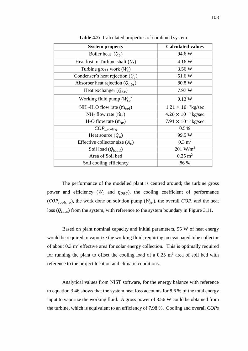
108
Table 4.2: Calculated properties of combined system
System property Calculated values
Boiler heat (𝑄𝑏) 94.6 W
Heat lost to Turbine shaft (𝑄𝑡) 4.16 W
Turbine gross work (𝑊𝑡) 3.56 W
Condenser’sنheatنrejectionن(𝑄𝑐) 51.6 W
Absorber heat rejection (𝑄𝑎𝑏𝑠) 80.8 W
Heat exchanger (𝑄ℎ𝑥) 7.97 W
Working fluid pump (𝑊𝑠𝑝) 0.13 W
NH3-H2O flow rate (ḿ𝑠𝑜𝑙) 1.21 × 10⁻⁴kg/sec
NH3 flow rate (ḿ𝑟) 4.26 × 10⁻⁵ kg/sec
H2O flow rate (ḿ𝑤) 7.91 × 10⁻⁵ kg/sec
COP_cooling 0.549
Heat source (𝑄𝑢) 99.5 W
Effective collector size (𝐴𝑐) 0.3 m2
Soil load (𝑄𝑙𝑜𝑎𝑑) 201 W/m2
Area of Soil bed 0.25 m2
Soil cooling efficiency 86 %
The performance of the modelled plant is centred around; the turbine gross
power and efficiency (𝑊𝑡 and 𝜂𝑂𝑅𝐶), the cooling coefficient of performance
(𝐶𝑂𝑃𝑐𝑜𝑜𝑙𝑖𝑛𝑔), the work done on solution pump (𝑊𝑠𝑝), the overall COP, and the heat
loss (𝑄𝑙𝑜𝑠𝑠) from the system, with reference to the system boundary in Figure 3.11.
Based on plant nominal capacity and initial parameters, 95 W of heat energy
would be required to vaporize the working fluid; requiring an evacuated tube collector
of about 0.3 m2 effective area for solar energy collection. This is optimally required
for running the plant to offset the cooling load of a 0.25 m2 area of soil bed with
reference to the project location and climatic conditions.
Analytical values from NIST software, for the energy balance with reference
to equation 3.46 shows that the system heat loss accounts for 8.6 % of the total energy
input to vaporize the working fluid. A gross power of 3.56 W could be obtained from
the turbine, which is equivalent to an efficiency of 7.98 %. Cooling and overall COPs

109
of 0.549 and 0.566, respectively, are achievable from the modelled system based on
the initial specifications and operating parameters.
4.3.2 Cooling Production
The evaporation taking place at condition 4–5 of the Figure 3.9 is caused by
exchange of heat between the working fluid (NH3) and the chilled water flowing
through the evaporator space (Baniyounes et al., 2013) before the absorption of the
working fluid by the low-pressure absorbent in section 5–6 of the same Figure.
Temperature of the chilled water is designed to vary between 5 ⁰C and 10 ⁰C, with the
minimum temperature corresponding to the maximum temperature of the refrigerant
at the exit from the evaporator space. Flow rate of the chilled water obtainable from
the evaporator is determined using equation (3.35). An average flow rate of 0.282
kg/min of chilled water could be obtained from the evaporator if inlet chilled water
temperature is maintained at 10 ⁰C.
4.3.3 Daytime Soil Cooling
Since the modelled systems (soil load and plant capacity) are based on the
nominal values of load and plant cooling capacity, the performance of the modelled
cooling system is affected by variations in the peak cooling load during the daytime.
It is also considered that in the absence of external heat source (solar radiation heat)
on the soil, its temperature gradient decays over time, leading to a thermal equilibrium
within the soil bed (∆𝑇 = 0, thus; 𝑄𝑐𝑜𝑛𝑑 ≈ 0); bringing the conductive heat flux close
to zero. Thus the soil cooling analysis presented in this study is basically focused on
the daytime, during which the thermal load affects the soil temperature. Soil cooling
efficiency is calculated as;
𝜂𝑆𝑜𝑖𝑙 𝐶𝑜𝑜𝑙𝑖𝑛𝑔 = [1 −(𝑃𝑒𝑎𝑘 𝐿𝑜𝑎𝑑)−(𝐶𝑜𝑜𝑙𝑖𝑛𝑔 𝐶𝑎𝑝𝑎𝑐𝑖𝑡𝑦)
(𝑃𝑒𝑎𝑘 𝑙𝑜𝑎𝑑)] × 100 (4.1)

110
Furthermore, using the solar radiation data from NASA (as contained in
Appendix A, soil temperature was studied for the period of 7:00hr and 19:00hr of the
day within which the solar radiation heat affects the soil. The key factor affecting soil
temperature is the soil solar radiation imposed load which also varies with the time of
the day. Therefore, with respect to the soil bed size in this study, chilled water flow
rates between 0.06 kg/min to 0.6 kg/min were selected to for the cooling process and
their effects were observed for optimal performance in offsetting the load, using
equation 3.45. The cooled soil temperature profile, shown in Figure 4.1 indicates the
effects of the mid-day peak load on the cooling performance based on the selected
chilled water flow rates. It however shows that the performance of the soil cooling
with the selected chilled water flow rates is affected by daytime peak load.
Figure 4.1: Modelled soil temperatures profile during daytime at different chilled
water flowrates
-60
-40
-20
0
20
40
60
80
100
120
140
0
5
10
15
20
25
30
35
Soil
pea
k l
oad
(W
)
Tem
per
ature
(℃
)
Daytime (hr)
Amb Air Temp Ts @ m = 0.24 kg/min Ts @ m = 0.6 kg/min
Ts @ m = 0.06 kg/min Peak load

111
4.4 Experimental Results
4.4.1 Cooling Production
Experimental runs were carried out on the investigated chiller by taking the
temperature profiles of its working fluid across its components to determine its steady
state energy balance and performance characteristics. Chilled water production was
achievedنfromنtheنchiller’sنevaporator, whose cooling rates were used to determine the
chilled water production rates as shown Figure 4.2.
Figure 4.2: Absorption chiller’sنoperatingنtemperature profile
In all the experimental runs, condenser temperature varied between 30 ºC and
35 ºC whereas the evaporator temperature was observed to range between -10 ºC and
-24 ºC with the average steady state value of about -18 ºC (Appendix F); corresponding
to working fluid saturated vapour of 2 bar.
It was observed that the cooling effects in the evaporator commenced when the
working fluid temperature reached about 61 ºC in the boiler. At this point, the
evaporator temperature reduced from ambient value of 29.44 ºC to 27.28 ºC. With
continuous heating, the steady state was reached at about 85 ºC of the working fluid
-40
-20
0
20
40
60
80
100
1 4 7 10 13 16 19 22 25 28 31 34 37 40 43 46 49 52 55 58 61Tem
per
ature
(ºC
)
Time (min)
T_evap T_amb air T_boiler
T_cond T_abs T_hx
112
temperature; corresponding to evaporator, ambient air, condenser, absorber, and
solution heat exchanger temperatures of -19.8 ºC, 29.7 ºC, 33.3 ℃, 37.1 ºC, and 56 ºC,
respectively. The cycle thermodynamic properties at these stages were used for the
analysis of the system.
To determine the chilled water production rate, the evaporator operating
characteristics was analysed. By integrating (conceptual) chilled water tank (with sets
of inlet and outlet chilled water temperatures) with the evaporator, the mass flow rates
of the chilled water were determined through the heat exchange between the chilled
water and the evaporator. Chilled water flow rates were determined using equation 4.2,
given as;
ḿ𝑤 =ḿ𝑟𝐶𝑝𝑟∆𝑇𝑟
𝐶𝑝𝑤∆𝑇𝑤 (4.2)
Where ḿ𝑟 and ḿ𝑤are the respective flow rates of refrigerant and chilled water, 𝐶𝑝𝑟
and 𝐶𝑝𝑤 are the respective heat capacities of refrigerant and water, and ∆𝑇𝑟 and ∆𝑇𝑤
are the respective change in refrigerant and water temperatures due to heat exchange
in the evaporator
From Figure 4.3, the experimental chiller gave an average chilled water flow
rate of 0.3 kg/min (18 kg/hr.), keeping the chilled water temperatures at the exit and
inlet of the chiller are at an average of 5 ºC and 10 ºC, respectively. The chilled water
and refrigerant exit temperatures from the evaporator were assumed equal.

113
Figure 4.3: Calculated chilled water flow rate set at 5 ºC
However, at its steady state when the boiler temperature was 85 ºC, the energy
balances across each of the components were determined as shown in Table 4.3. This
gaveنchiller’sنcoefficient of performance of 0.56. The mass flow rates of the working
fluidsنwereنdeterminedنbasedنonنtheنchiller’sنnominalنcapacity and working fluid mass
fraction.
Table 4.3: Calculated chiller energy balance at steady state
Components Temperature Energy Balance
Boiler 85 90.06
Condenser 33 55.62
Evaporator -19 50.0
Absorber 34 85.0
Bubble pump 85 0.24
4.4.2 Soil Temperature Profile
To cool the soil to the set range of temperatures, chilled water temperatures to
the soil bed were maintained between 2.5 ºC and 10 ºC, while the flow rates were
varied from 0.24 kg/min to 0.6 kg/min. The effects of the chilled water flow rates were
observed on the cooled soil and compared with that of the control soil bed. For
0
0.05
0.1
0.15
0.2
0.25
0.3
0.35
Ch
ille
d W
ate
r F
low
Ra
te (
kg
/min
)
Evaporator Temperature (⁰C)

114
offsetting the cooling load of the soil bed in this study, Figure 4.4 (A – D) show that
the selected flow rates fall within the required rate. While the chilled water flow rate
of 0.24 kg/min (Figure 4.4 A) was only sufficient in the morning and evening periods
(during minimum load), 0.36 kg/min and 0.48 kg/min were observed to be optimally
sufficient during the whole study periods. However, higher chilled water flow rate
(0.6 kg/min) was only be required during the mid-day peak load, which corresponds
to 10:00hr and 16:30hr clock time of the day as shown in Figure 4.4 D. During this
period, the cooling system may be required to operate at maximum capacity.
Figure 4.4: Experimental soil temperature profiles at different chilled water flow
rates
However, besides the chilled water flow rates and temperatures, the effects of
daytime weather condition were observed on the soil temperature profile during the
mid-day, when the air temperature and solar radiation were at the peak. For this,
analyses of factors and responses were conducted, using RMS ofنtheن“DesignنExpert®,
05
1015202530354045
Tem
per
atu
re (
ºC)
Daytime (hr)
T_C.W inlet T_Amb airT_Contr soil T_Cooled soil
05
1015202530354045
Tem
per
atu
re (
ºC)
Daytime (hr)
T_C.W inlet T_Amb airT_Contr soil T_Cooled soil
05
1015202530354045
Tem
per
atu
re (
ºC)
Daytime (hr)
T_CW inlet T_Amb airT_Contr soil T_Cooled soil
05
1015202530354045
Tem
per
atu
re (
ºC)
Daytime (hr)
T_C.W Inlet T_Amb airT_Contr soil T_Cooled soil
D: (0.6 kg/min. Flow rate) C: (0.48 kg/min. Flow rate)
A: (0.24 kg/min. Flow rate)
B: (0.36 kg/min. Flow rate)
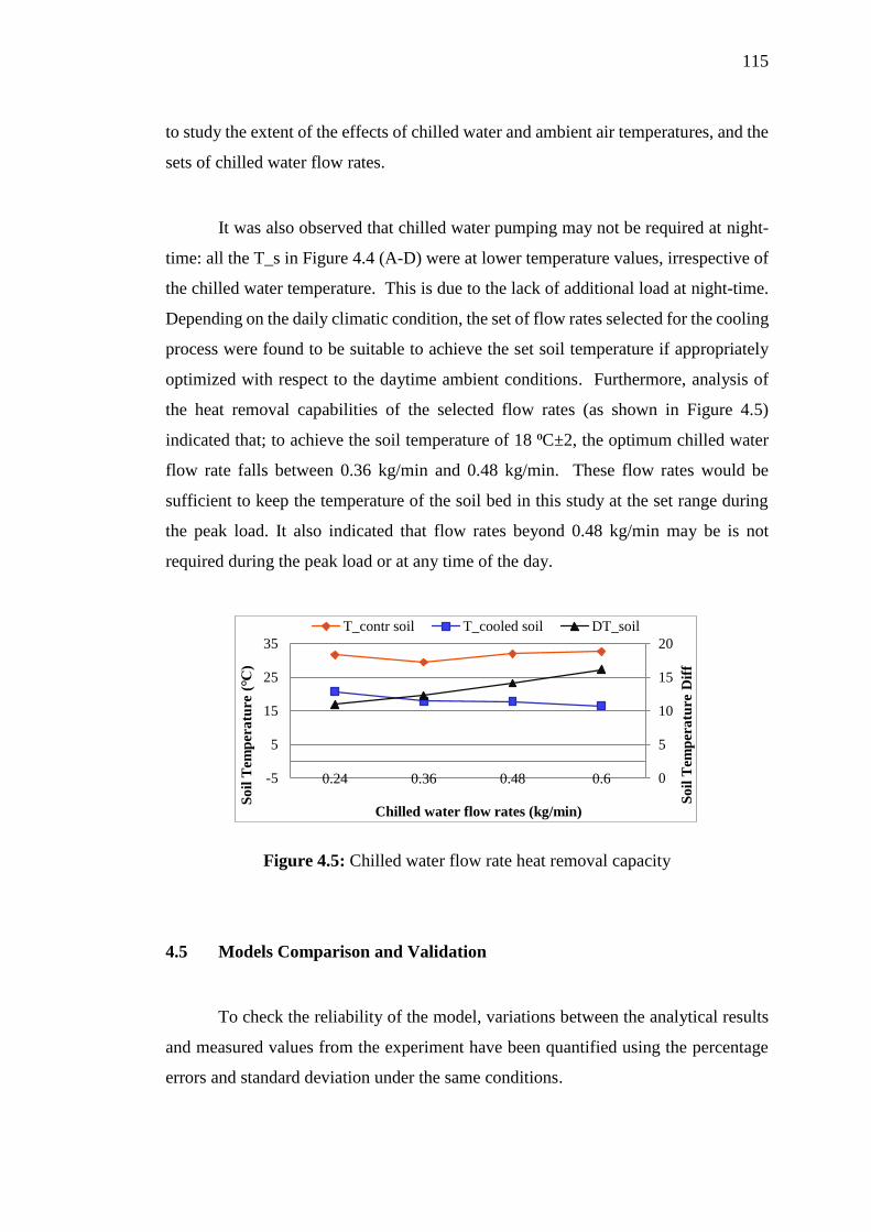
115
to study the extent of the effects of chilled water and ambient air temperatures, and the
sets of chilled water flow rates.
It was also observed that chilled water pumping may not be required at night-
time: all the T_s in Figure 4.4 (A-D) were at lower temperature values, irrespective of
the chilled water temperature. This is due to the lack of additional load at night-time.
Depending on the daily climatic condition, the set of flow rates selected for the cooling
process were found to be suitable to achieve the set soil temperature if appropriately
optimized with respect to the daytime ambient conditions. Furthermore, analysis of
the heat removal capabilities of the selected flow rates (as shown in Figure 4.5)
indicated that; to achieve the soil temperature of 18 ⁰C±2, the optimum chilled water
flow rate falls between 0.36 kg/min and 0.48 kg/min. These flow rates would be
sufficient to keep the temperature of the soil bed in this study at the set range during
the peak load. It also indicated that flow rates beyond 0.48 kg/min may be is not
required during the peak load or at any time of the day.
Figure 4.5: Chilled water flow rate heat removal capacity
4.5 Models Comparison and Validation
To check the reliability of the model, variations between the analytical results
and measured values from the experiment have been quantified using the percentage
errors and standard deviation under the same conditions.
0
5
10
15
20
-5
5
15
25
35
0.24 0.36 0.48 0.6
So
il T
emp
era
ture
Dif
f
So
il T
emp
era
ture
(℃
)
Chilled water flow rates (kg/min)
T_contr soil T_cooled soil DT_soil

116
4.5.1 Modelled and Experimental Soil Cooling Rates
This section of the thesis is focused on the comparison of the daytime soil
temperature profiles. The comparison is based on the results of the analytical and
experimental models soil cooling processes, using the same chilled water inlet
temperatures and flow rates. Figure 4.6 (A–D) show the comparison of experimental
and modelled soil cooling temperature profiles with different chilled water flow rates
and temperatures, and at different ambient air temperatures.
Figure 4.6: Experimental and modelled soil temperature profiles for different chilled
water flow rates
Both the experimental and modelled soil temperatures were observed to
respond to chilled water flow rates and temperatures, and the ambient conditions of
each of the experimental days. The modelled soil temperatures in Figure 4.6 D were
however lower than the experimental values. This is due partly to some simplification
assumptions in the modelling and the use of historical climatic data for the peak load
05
1015202530354045
Tem
per
atu
re (
ºC)
Daytime (hr)
T_C.W inlet T_Amb airTs_Model Ts_Exp
05
1015202530354045
Tem
per
atu
re (
ºC)
Daytime (hr)
T_C.W inlet T_Amb airTs_Model Ts_Exp
05
1015202530354045
Tem
per
atu
re (
ºC)
Daytime (hr)
T_C.W inlet Amb AirTs_Model Ts_Exp
05
1015202530354045
Tem
per
atu
re (
ºC)
Daytime (hr)
T_C.W Inlet T_Amb airTs_(model) Ts_(exp)
D: (0.6 kg/min)
A; (0.24 kg/min) B: (0.36 kg/min)
C: (0.48 kg/min)
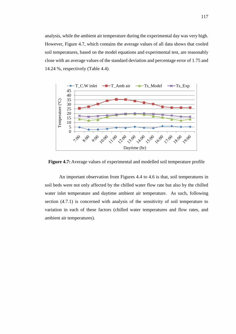
117
analysis, while the ambient air temperature during the experimental day was very high.
However, Figure 4.7, which contains the average values of all data shows that cooled
soil temperatures, based on the model equations and experimental test, are reasonably
close with an average values of the standard deviation and percentage error of 1.75 and
14.24 %, respectively (Table 4.4).
Figure 4.7: Average values of experimental and modelled soil temperature profile
An important observation from Figures 4.4 to 4.6 is that, soil temperatures in
soil beds were not only affected by the chilled water flow rate but also by the chilled
water inlet temperature and daytime ambient air temperature. As such, following
section (4.7.1) is concerned with analysis of the sensitivity of soil temperature to
variation in each of these factors (chilled water temperatures and flow rates, and
ambient air temperatures).
05
1015202530354045
Tem
per
ature
(ºC
)
Daytime (hr)
T_C.W inlet T_Amb air Ts_Model Ts_Exp

118
Table 4.4: Experimental and model soil temperature comparison
Time
(hr)
C.W Inlet
Temp (ºC)
Soil Temp (ºC) % Error STDev
Exp. Model
7:00 4.74 17.31 13.61 21.39 2.62
8:00 2.13 16.50 12.32 17.53 2.96
9:00 2.28 17.05 13.24 27.76 2.69
10:00 3.00 17.88 16.06 25.97 1.29
11:00 4.29 18.65 18.18 13.89 0.33
12:00 3.92 19.55 19.15 6.98 0.28
13:00 5.27 19.98 19.47 4.18 0.36
14:00 4.12 19.92 18.76 2.27 0.82
15:00 3.74 19.28 17.14 2.69 1.51
16:00 6.01 18.47 15.58 7.17 2.04
17:00 6.06 17.72 13.49 12.10 2.30
18:00 5.12 16.55 12.26 18.53 3.04
19:00 5.28 16.26 13.66 24.62 1.84
Average 4.30 18.09 15.61 14.24 1.75
4.5.2 Modelled and Experimental Chilled Water System
The modelled plant and the experimental chiller were compared with respect
to their coefficient of performance, using an ideal absorption cooling cycle COP, and
comparing with the present model using REFPROP. The assessment of the
experimental chiller is based on its temperature profile during operation, thus
coefficient of performance has been analysed based on system operating temperature
using the relation in equation 3.61 (Gordon and Ng, 1995).
Some approximations were made to give room for the analysis of the COP of
the studied chiller: these include;
i. Once the steady state is reached, absorption chillers normally operate
within a close range of boiler temperatures (Gordon and Ng, 1995; Miles
et al., 1993), as such, analysis in this study only considered the boiler’s

119
operation between 82ºC and 90 ºC within which the steady state has been
established.
ii. Since the chiller was insulated against the ambient environment, losses in
the system (from Equation 3.62) that occurred from the air-cooled
condenser and absorber have been approximated to 5 % of the heat input.
Meanwhile, it is required that same operating conditions be set for both
simulated/analytical and experimental setup for them to be reasonably compared
(Massaguer. et al., 2014). Thus the cooling COP for the experimental chiller, based
on measured data and modelled equation has been considered under the same operating
temperature, pressure and working fluid flow rates and mass fraction.
Table 4.5: Experimental & modelled chiller’sنCOP comparison
T_boiler (ºC) COP_cooling
% Error STDev Exp. Model
82 0.528 0.561 5.882 0.023
83 0.507 0.560 9.464 0.037
84 0.500 0.558 10.394 0.041
85 0.493 0.555 11.171 0.044
86 0.489 0.553 11.573 0.045
87 0.497 0.549 9.472 0.037
88 0.506 0.547 7.495 0.029
89 0.513 0.544 5.698 0.022
90 0.520 0.539 3.525 0.013
Averages 0.506 0.552 8.297 0.032
The comparison of the COP of the chiller, based on the measured data and
model equations using REFPROP, is presented in Table 4.5 with average percentage
error of 8.30 and standard deviation of 0.03; showing strong agreement in
performances between measured data and modelled data. This shows that the modelled
equation with the thermodynamic properties of the working fluid, using REFPROP is
suitable to reasonably predict the performances of the system.

120
4.5.3 Component Analysis of the Experimental Chiller
The analysis of the experimental chiller was done, using the temperature data
obtained during its steady state operation. The data were combined with its capacity
and other nominal details and used to determine other thermodynamic properties of the
chiller. The thermodynamic properties calculated with REFPROP are presented in
Table 4.6.
Table 4.6: Calculated working fluid thermodynamic properties of experimental
chiller
Components Temp
(ºC)
Press
(bar)
h
(KJ/Kg)
Internal
Energy (kJ/kg)
S
(KJ/Kg-K)
V
(m3/kg)
Boiler 85 16 1766.60 1607.10 6.0139 0.09969
Condenser 33 16 499.57 496.86 2.0054 0.00169
Evaporator -19 2 256.23 255.93 1.1431 0.00151
Absorber 34 2 41.40 41.17 0.8446 0.00115
Heat
Exchanger 54 16 132.50 130.62 1.1267 0.00117
P inlet = 16 bar NH3:H2O Ratio = 35:65
At the selected stages of the chiller, mass and energy balances across the major
components showed that the heat gained by the working for vaporization is 90.1 W,
while the heat rejection of 55.6 W and 85 W occurred from the condenser and absorber,
respectively. Only 0.2 W of energy was expended on the bubble pump to create
pressure increase at the boiler section. However, the condenser and absorber are air-
cooled; requiring the application of 2.5 W (USB) mini-fan to improve their cooling
performances: this increased the electrical energy requirement of the system to 2.7 W.
The amount of heat to vaporize the working fluid required an evacuated solar collector
(with 95 % thermal efficiency) size of 0.29 m2, with reference to the available solar
radiation at the experimental location.

121
4.5.4 Combined Plant Analysis
The combined plant is the modified chiller with the integration of organic
Rankine turbine, as shown in Figure 3.9. Under the same operating conditions at the
boiler with the experimental chiller, the inclusion of the ORC turbine reduced the
temperature and pressure of the condenser, thus, the working fluid characteristics at
the condenser results in the few observable changes between the experimental chiller
and the combined plant. The coefficient of performance of the chiller and the
efficiency of the ORC were also determined differently from the conventional
approaches. Table 4.7 shows the thermodynamic properties of the combined plant and
its working fluid.
Table 4.7: Working fluid thermodynamic properties of combined plant
Stage Temp
(ºC)
Pressure
(bar)
h
(KJ/Kg)
Internal Energy
(kJ/kg)
S
(KJ/Kg-K)
V
(m3/kg)
Boiler 85 16 1766.6 1607.1 6.0139 0.09969
Turbine 40 10 1671.3 1532.7 5.9383 0.13866
Condenser 25 10 460.82 1498.1 1.8804 0.1286
Evaporator -19 2 256.23 255.93 1.1431 0.00151
Absorber 34 2 41.402 41.172 0.84457 0.00115
Heat
Exchanger 54 16 132.5 130.62 1.1267 0.00117
P inlet = 16 bar NH3:H2O = 35:65
Energy expended due to expansion through the ORC turbine is equivalent to
3.535 W of gross power output. As shown in Table 4.8, about 7.52 % reduction in the
heat rejection by the condenser (from 55.6 W in the experimental chiller to 51.44 W
in the combined plant) was also observed. However, since the working fluid is the
same, in type and composition, and the two systems use the same process path, energy
balance at other components remain the same.
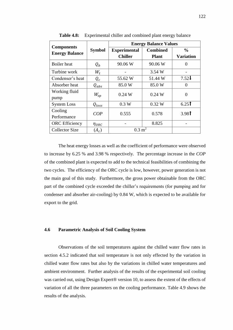
122
Table 4.8: Experimental chiller and combined plant energy balance
Components
Energy Balance Symbol
Energy Balance Values
Experimental
Chiller
Combined
Plant
%
Variation
Boiler heat 𝑄𝑏 90.06 W 90.06 W 0
Turbine work 𝑊𝑡 - 3.54 W -
Condenser’sنheatن 𝑄𝑐 55.62 W 51.44 W 7.52⬇
Absorber heat 𝑄𝑎𝑏𝑠 85.0 W 85.0 W 0
Working fluid
pump 𝑊𝑠𝑝 0.24 W 0.24 W 0
System Loss 𝑄𝑙𝑜𝑠𝑠 0.3 W 0.32 W 6.25⬆
Cooling
Performance COP 0.555 0.578 3.98⬆
ORC Efficiency 𝜂𝑂𝑅𝐶 - 8.825 -
Collector Size (𝐴𝑐) 0.3 m2
The heat energy losses as well as the coefficient of performance were observed
to increase by 6.25 % and 3.98 % respectively. The percentage increase in the COP
of the combined plant is expected to add to the technical feasibilities of combining the
two cycles. The efficiency of the ORC cycle is low, however, power generation is not
the main goal of this study. Furthermore, the gross power obtainable from the ORC
part of the combined cycle exceeded the chiller’sنrequirementsن(forنpumping and for
condenser and absorber air-cooling) by 0.84 W, which is expected to be available for
export to the grid.
4.6 Parametric Analysis of Soil Cooling System
Observations of the soil temperatures against the chilled water flow rates in
section 4.5.2 indicated that soil temperature is not only effected by the variation in
chilled water flow rates but also by the variations in chilled water temperatures and
ambient environment. Further analysis of the results of the experimental soil cooling
was carried out, using Design Expert® version 10, to assess the extent of the effects of
variation of all the three parameters on the cooling performance. Table 4.9 shows the
results of the analysis.

123
Table 4.9: Factors and response on soil cooling analysis
Run
Factors Response
Amb Air
Temp (℃)
Chilled water
Temp (℃)
Chilled water Flow
Rates (kg/min) T_s (℃)
1 31.5 8.5 0.48 19.05
2 25.5 2.5 0.36 17.60
3 31.5 8.5 0.36 19.98
4 31.0 3.5 0.24 19.29
5 25.0 5.5 0.36 18.57
6 35.0 5.0 0.60 17.27
7 31.0 3.5 0.24 19.29
8 25.0 4.5 0.48 17.29
9 27.0 8.5 0.60 17.77
10 31.5 8.5 0.36 19.98
11 35.5 4.5 0.48 18.06
12 31.5 7.5 0.48 18.72
13 35.0 4.5 0.24 19.89
14 29.0 7.5 0.60 17.61
15 25.0 5.5 0.36 18.55
16 25.0 4.8 0.60 16.46
17 26.5 4.5 0.36 18.34
18 35.5 4.5 0.60 17.13
19 29.0 7.5 0.36 19.47
20 25.0 4.5 0.36 18.23
As contained in Appendix G1-1, the overview of the factors-responses
correlations of 0.210, 0.256, and 0.572 for ambient air temperature, chilled water
temperature, and chilled water flow rate respectively, indicated that the effects of
chilled water flow rates is the most significant on cooled soil temperature (T_s), while
those of the ambient air and chilled water temperatures are fairly similar in
significance. The analysis of variance (ANOVA) performed to find out the
interactions of the factors and responses showed that the model is significant. The
model has F and p values of 7.09 and 0.0030, respectively,نandن“Lack of Fit”نwith p
and F values of 2.14 and 0.299. The Lack of Fit is not significant; indicating that the
model is good. The regression equation developed from the ANOVA for the soil
temperature (T_s) is given in equation 4.3 as;
𝑇𝑠 = 17.777 + 0.073 (𝐴) + 0.318(𝐵) − 466.693(𝐶) (4.3)
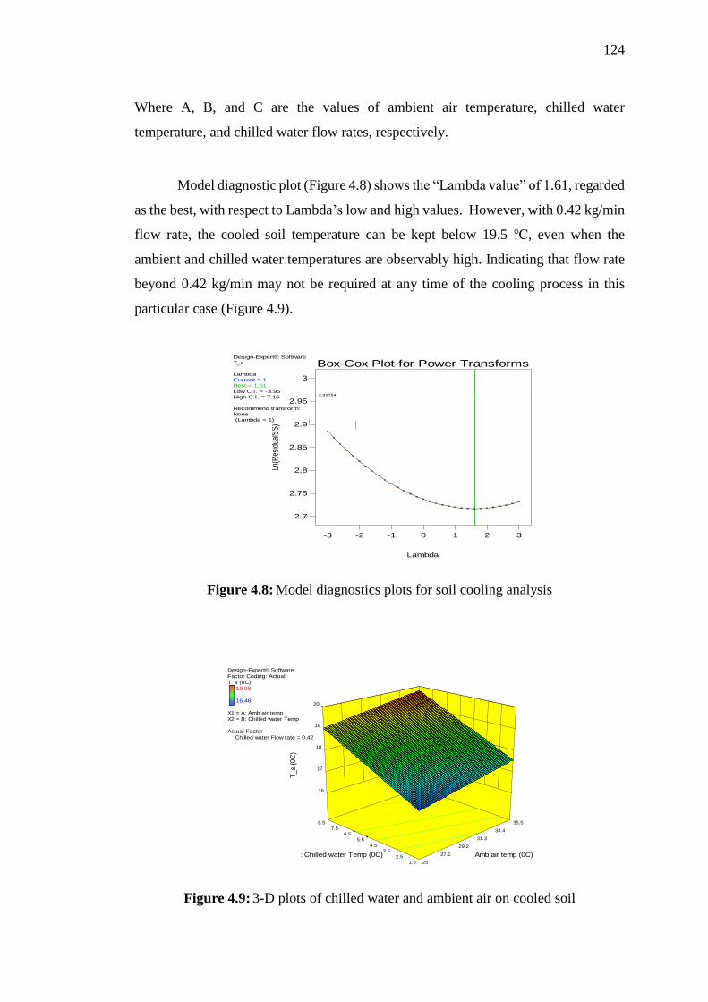
124
Where A, B, and C are the values of ambient air temperature, chilled water
temperature, and chilled water flow rates, respectively.
Model diagnostic plot (Figure 4.8)نshowsنtheن“Lambdaنvalue”نof1.61ن, regarded
as the best, with respect to Lambda’s low and high values. However, with 0.42 kg/min
flow rate, the cooled soil temperature can be kept below 19.5 ℃, even when the
ambient and chilled water temperatures are observably high. Indicating that flow rate
beyond 0.42 kg/min may not be required at any time of the cooling process in this
particular case (Figure 4.9).
Figure 4.8: Model diagnostics plots for soil cooling analysis
Figure 4.9: 3-D plots of chilled water and ambient air on cooled soil
Design-Expert® Software
T_s
Lambda
Current = 1
Best = 1.61
Low C.I. = -3.95
High C.I. = 7.16
Recommend transform:
None
(Lambda = 1)
Lambda
Ln(R
esid
ualS
S)
Box-Cox Plot for Power Transforms
2.7
2.75
2.8
2.85
2.9
2.95
3
-3 -2 -1 0 1 2 3
2.95754
Design-Expert® Software
T_s
Lambda
Current = 1
Best = 1.61
Low C.I. = -3.95
High C.I. = 7.16
Recommend transform:
None
(Lambda = 1)
Lambda
Ln(R
esid
ualS
S)
Box-Cox Plot for Power Transforms
2.7
2.75
2.8
2.85
2.9
2.95
3
-3 -2 -1 0 1 2 3
2.95754
Design-Expert® SoftwareFactor Coding: ActualT_s (0C)
19.98
16.46
X1 = A: Amb air tempX2 = B: Chilled water Temp
Actual FactorC: Chilled water Flow rate = 0.42
1.5
2.5
3.5
4.5
5.5
6.5
7.5
8.5
25
27.1
29.2
31.3
33.4
35.5
16
17
18
19
20
T_s
(0C
)
A: Amb air temp (0C)B: Chilled water Temp (0C)
Design-Expert® SoftwareFactor Coding: ActualT_s (0C)
19.98
16.46
X1 = A: Amb air tempX2 = B: Chilled water Temp
Actual FactorC: Chilled water Flow rate = 0.42
1.5
2.5
3.5
4.5
5.5
6.5
7.5
8.5
25
27.1
29.2
31.3
33.4
35.5
16
17
18
19
20
T_s
(0C
)
A: Amb air temp (0C)B: Chilled water Temp (0C)

125
4.7 Parametric Analysis of Combined Plant
The analysed system in section 4.6.4 was based on the selected parameters of
the combined plant. However, the performance of the plant (gross power output,
pumping power, heat loss, cooling COP, ORC efficiency, and the overall COP) can be
improved by careful selection of the key operation parameters (Yang. et al., 2015).
Furthermore, it has also been reported that, in designing combined systems (such as
CHP, CCHP and CCP), determining the best configuration with respect to the
thermodynamics of all subsystems and overall energy efficiency is considered very
critical (Maraver et al., 2013) right from the initial stage of the project.
In this study, improvement of the plant performance has been carried out
through the parametric analysis, using RSM. Table 4.10 shows the results of analysis
of the key parameters of interest (working fluid mass fraction,نboiler’sنpressure,نandن
working fluid vaporizing temperature). Effects of these parameters on the plant
performance are presented in the following sections of the thesis.

126
Table 4.10: Factors and response on combined plant analysis
Run
Factors Responses
W/F
Temp
(ºC)
Boiler
Press
(bar)
W/F
C.R
W_t
(kW)
W_sp
(kW)
Q_loss
(kW) COP_cooling ORC_eff COP_overall
1 65 12 0.65 0.00213 0.00008 0.00042 0.677 8.551 0.721
2 85 21 0.45 0.00403 0.00023 0.00644 0.590 10.398 0.628
3 65 15 0.45 0.00212 0.00016 0.00167 0.624 6.578 0.657
4 80 21 0.6 0.00356 0.00018 0.00208 0.649 11.628 0.687
5 90 15 0.35 0.00450 0.00021 0.01227 0.529 9.183 0.566
6 100 12 0.5 0.00542 0.00011 0.00779 0.589 13.466 0.635
7 100 21 0.65 0.00542 0.00016 0.00358 0.643 16.338 0.688
8 85 15 0.65 0.00403 0.00011 0.00185 0.657 13.386 0.698
9 100 12 0.5 0.00542 0.00011 0.00779 0.589 13.466 0.635
10 100 18 0.3 0.00542 0.00029 0.02023 0.475 8.936 0.516
11 80 12 0.3 0.00356 0.00018 0.01145 0.518 7.095 0.553
12 70 12 0.4 0.00260 0.00014 0.00388 0.595 7.118 0.629
13 65 21 0.3 0.00212 0.00035 0.00512 0.555 4.856 0.583
14 90 18 0.55 0.00450 0.00016 0.00455 0.621 12.868 0.663
15 90 18 0.55 0.00450 0.00016 0.00185 0.628 13.386 0.665
16 85 21 0.45 0.00403 0.00023 0.00644 0.590 10.398 0.629
17 100 18 0.3 0.00542 0.00029 0.02023 0.475 8.936 0.516
18 65 15 0.45 0.00212 0.00016 0.00167 0.625 6.578 0.657
19 65 15 0.45 0.00212 0.00018 0.00512 0.623 6.126 0.656
20 65 21 0.65 0.00212 0.00016 0.00034 0.677 8.151 0.710
21 80 15 0.5 0.00356 0.00014 0.00392 0.618 10.310 0.666
22 80 15 0.45 0.00356 0.00016 0.00167 0.625 9.659 0.657
23 85 15 0.65 0.00403 0.00011 0.00185 0.657 13.385 0.688
Factors-responses correlations gave the general overview of the sensitivity of
each of the factors on the performances of the plant (as shown in Table 4.11). The
model generally showed that, increasing the working fluid vaporizing temperature only
favours the ORC part at the expense of the cooling performances. Meanwhile, in this
study, cooling is the primary goal, requiring some trade-offs to achieve overall system
optimal performance.

127
Table 4.11: Factors-responses correlations for combined plant
Factor Response Correlation
Working fluid
vaporizing
temperature
(W/F Temp)
Gross Power (W_t) 1.000
Pump Power (W_sp) 0.072
Heat Loss (Q_loss) 0.579
COP_cooling -0.429
ORC_eff 0.728
COP_overall -0.357
Boiler’sنpressureن
(Boiler Press)
Gross Power (W_t) 0.066
Pump Power (W_sp) 0.586
Heat Loss (Q_loss) 0.005
COP_cooling 0.017
ORC_eff 0.102
COP_overall 0.015
Working fluid mass
fraction (C.R)
Gross Power (W_t) -0.055
Pump Power (W_sp) -0.723
Heat Loss (Q_loss) -0.738
COP_cooling 0.904
ORC_eff 0.606
COP_overall 0.929
Variations in boiler pressure only significantly affected the pumping power
requirements, with no significant effects on other outputs of the plant. This correlates
with the studies by (Al-Sulaiman. et al., 2012) in which the effects of variation in
turbine inlet pressure was insignificant and it was concluded that ORC turbine could
be run on low pressure to save cost.
Variation in the working fluid mass fraction significantly and positively
correlated with the cooling performance. It however correlated negatively with heat
loss and pumping power, and insignificantly, negatively correlated with the gross
power output.
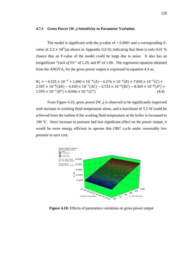
128
4.7.1 Gross Power (W_t) Sensitivity to Parameter Variation
The model is significant with the p-value of < 0.0001 and a corresponding F-
value of 2.2 × 10⁷(as shown in Appendix G2-3); indicating that there is only 0.01 %
chance that an F-value of the model could be large due to noise. It also has an
insignificant “Lack of Fit” of 1.29, and R2 of 1.00. The regression equation obtained
from the ANOVA, for the gross power output is expressed in equation 4.4 as;
𝑊𝑡 = −4.525 × 10⁻³ + 1.080 × 10⁻⁴(𝐴) − 6.276 × 10⁻⁶(𝐵) + 7.830 × 10⁻⁵(𝐶) +
2.587 × 10⁻⁸(𝐴𝐵) − 4.430 × 10⁻⁷(𝐴𝐶) − 2.723 × 10⁻⁶(𝐵𝐶) − 8.369 × 10⁻⁸(𝐴2) +
1.595 × 10⁻⁷(𝐵2) + 8.046 × 10⁻⁶(𝐶2) (4.4)
From Figure 4.10, gross power (W_t) is observed to be significantly improved
with increase in working fluid temperature alone, and a maximum of 5.5 W could be
achieved from the turbine if the working fluid temperature at the boiler is increased to
100 ℃. Since increase in pressure had less significant effect on the power output, it
would be more energy efficient to operate this ORC cycle under reasonably low
pressure to save cost.
Figure 4.10: Effects of parameters variations on gross power output
Design-Expert® Software
Factor Coding: Actual
W_t (W)
0.0054234
0.0021162
X1 = A: W/F Temp
X2 = B: Boiler Press
Actual Factor
C: W/F C.R = 0.475
12 13
14 15
16 17
18 19
20 21
65 72
79 86
93 100
0.002
0.003
0.004
0.005
0.006
W_t
(W
)
A: W/F Temp (C)B: Boiler Press (Bar)
Design-Expert® Software
Factor Coding: Actual
W_t (W)
0.0054234
0.0021162
X1 = A: W/F Temp
X2 = B: Boiler Press
Actual Factor
C: W/F C.R = 0.475
12 13
14 15
16 17
18 19
20 21
65 72
79 86
93 100
0.002
0.003
0.004
0.005
0.006
W_t
(W
)
A: W/F Temp (C)B: Boiler Press (Bar)

129
4.7.2 Pumping Power (W_sp) Sensitivity to Parameter Variation
The model is significant with the p-value of < 0.0001 and a corresponding F-
value of 190.57, meaning that there is less than 0.01 % chance that an F-value of the
model could be large due to noise. The mode has a non-significant “Lack of Fit” of
0.76, and R2 of 0.992, indicating that the model term is good. Similarly, the regression
equation obtained from the ANOVA for the pump energy consumption (W_sp) is
expressed in equation 4.5 as;
𝑊𝑠𝑝 = 1.702 × 10⁻⁴ − 2.848 × 10⁻⁶(𝐴) + 3.563 × 10⁻⁵(𝐵) − 7.567 × 10⁻⁴(𝐶) −
2.972 × 10⁻⁸(𝐴𝐵) + 6.189 × 10⁻⁷(𝐴𝐶) − 2.56 × 10⁻⁵(𝐵𝐶) + 1.806 × 10⁻⁸(𝐴2) −
2.576 × 10⁻⁷(𝐵2) + 7.631 × 10⁻⁴(𝐶2) (4.5)
However from Figure 4.11, effect of boiler pressure variation is observed to be
more significant on the energy required to pump working fluid, with the least
significant effect form the working fluid temperature. Thus, to minimize the pumping
power, lower boiler pressure is equally recommended in this case. This will also save
cost associated with high pressure operation.
Figure 4.11: Effects of parameters variations on solution pump
Design-Expert® Software
Factor Coding: Actual
W_sp (W)
0.0003492
8.48E-005
X1 = A: W/F Temp
X2 = B: Boiler Press
Actual Factor
C: W/F C.R = 0.475
12 13
14 15
16 17
18 19
20 21
65 72
79 86
93 100
5E-005
0.0001
0.00015
0.0002
0.00025
0.0003
0.00035
W_s
p (W
)
A: W/F Temp (C)B: Boiler Press (Bar)
Design-Expert® Software
Factor Coding: Actual
W_sp (W)
0.0003492
8.48E-005
X1 = A: W/F Temp
X2 = B: Boiler Press
Actual Factor
C: W/F C.R = 0.475
12 13
14 15
16 17
18 19
20 21
65 72
79 86
93 100
5E-005
0.0001
0.00015
0.0002
0.00025
0.0003
0.00035
W_s
p (W
)
A: W/F Temp (C)B: Boiler Press (Bar)
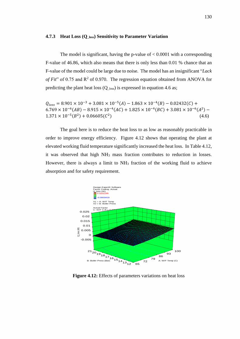
130
4.7.3 Heat Loss (Q_loss) Sensitivity to Parameter Variation
The model is significant, having the p-value of < 0.0001 with a corresponding
F-value of 46.86, which also means that there is only less than 0.01 % chance that an
F-value of the model could be large due to noise. The model has an insignificant “Lack
of Fit”نofن0.75نandنR2 of 0.970. The regression equation obtained from ANOVA for
predicting the plant heat loss (Q_loss) is expressed in equation 4.6 as;
𝑄𝑙𝑜𝑠𝑠 = 8.901 × 10⁻³ + 3.081 × 10⁻⁵(𝐴) − 1.863 × 10⁻⁴(𝐵) − 0.02432(𝐶) +
6.769 × 10⁻⁶(𝐴𝐵) − 8.915 × 10⁻⁴(𝐴𝐶) + 1.825 × 10⁻⁴(𝐵𝐶) + 3.081 × 10⁻⁶(𝐴2) −
1.371 × 10⁻⁵(𝐵2) + 0.06605(𝐶2) (4.6)
The goal here is to reduce the heat loss to as low as reasonably practicable in
order to improve energy efficiency. Figure 4.12 shows that operating the plant at
elevated working fluid temperature significantly increased the heat loss. In Table 4.12,
it was observed that high NH3 mass fraction contributes to reduction in losses.
However, there is always a limit to NH3 fraction of the working fluid to achieve
absorption and for safety requirement.
Figure 4.12: Effects of parameters variations on heat loss
Design-Expert® Software
Factor Coding: Actual
Q_loss (W)
0.0202295
-0.0003419
X1 = A: W/F Temp
X2 = B: Boiler Press
Actual Factor
C: W/F C.R = 0.475
12 13
14 15
16 17
18 19
20 21
65 72
79 86
93 100
-0.005
0
0.005
0.01
0.015
0.02
0.025
Q_l
oss
(W)
A: W/F Temp (C)B: Boiler Press (Bar)
Design-Expert® Software
Factor Coding: Actual
Q_loss (W)
0.0202295
-0.0003419
X1 = A: W/F Temp
X2 = B: Boiler Press
Actual Factor
C: W/F C.R = 0.475
12 13
14 15
16 17
18 19
20 21
65 72
79 86
93 100
-0.005
0
0.005
0.01
0.015
0.02
0.025
Q_l
oss
(W)
A: W/F Temp (C)B: Boiler Press (Bar)

131
4.7.4 Sensitivity on Cooling COP
The model is significant with the p-value of < 0.0001 and a corresponding F-
value of 1559.41, indicating that, there is only about 0.01 % chance that an F-value of
the model could be large due to noise. It also has an insignificant “Lack of Fit”نofن0.61ن
and R2 of 0.999. For the cooling COP, equation 4.7 expresses the regression equation
obtained from the ANOVA, which can be used to predict the cooling COP of the plant.
𝐶𝑂𝑃𝑐𝑜𝑜𝑙𝑖𝑛𝑔 = 0.53197 − 3.379 × 10⁻³(𝐴) + 1.426 × 10⁻³(𝐵) + 0.709(𝐶) − 2.918 ×
10−6(𝐴𝐵) + 3.708 × 10⁻³(𝐴𝐶) − 8.232 × 10⁻⁴(𝐵𝐶) + 4.066 × 10⁻⁷(𝐴2) − 2.349 ×
10−5(𝐵2) − 0.61498(𝐶2) (4.7)
From Figure 4.13,نbothنofنtheنworkingنfluidنtemperatureنandنboiler’sنpressureن
are observed to have negative effects on the cooling COP of the combined plant. Thus
it is recommended that plant be operated at moderate temperature and pressure for
optimal cooling COP.
Figure 4.13: Effects of parameters variations on cooling COP
Design-Expert® Software
Factor Coding: Actual
COP_cooling
0.677087
0.47497
X1 = A: W/F Temp
X2 = B: Boiler Press
Actual Factor
C: W/F C.R = 0.475
12 13
14 15
16 17
18 19
20 21
65 72
79 86
93 100
0.45
0.5
0.55
0.6
0.65
0.7
CO
P_co
olin
g
A: W/F Temp (C)B: Boiler Press (Bar)
Design-Expert® Software
Factor Coding: Actual
COP_cooling
0.677087
0.47497
X1 = A: W/F Temp
X2 = B: Boiler Press
Actual Factor
C: W/F C.R = 0.475
12 13
14 15
16 17
18 19
20 21
65 72
79 86
93 100
0.45
0.5
0.55
0.6
0.65
0.7
CO
P_c
oolin
g
A: W/F Temp (C)B: Boiler Press (Bar)

132
4.7.5 ORC Efficiency Sensitivity to Parameter Variation
The model is significant with the p-value of < 0.0001 and an F-value of 359.87.
It also has non-significant “Lack of Fit’نof1.05ن, and R2 of 0.993 which all indicated
that the model is good. The ANOVA regression equation for efficiency of the organic
Rankine cycle is expressed in equation 4.8 as;
𝑂𝑅𝐶𝑒𝑓𝑓 = −10.228 + +0.290(𝐴) − 0.226(𝐵) − 2.529(𝐶) + 8.321 × 10⁻⁴(𝐴𝐵) +
0.3241(𝐴𝐶) − 0.108(𝐵𝐶) − 1.70110−3(𝐴2) + 6.246 × 10⁻³(𝐵2) − 7.1142(𝐶2) (4.8)
Figure 4.14 shows that the working fluid temperature significantly affects the
ORC efficiency. This could also be observed in Table 4.11 where the response of ORC
efficiency to factors is highest with the working fluid temperature, with a value of
0.728.
Figure 4.14: Effects of parameters variations on ORC efficiency
4.7.6 Overall COP Sensitivity to Parameter Variation
The model is significant, having the p-value of < 0.0001 with a corresponding
F-value of 579.26. It also has an insignificant “Lack of Fit”نofن1.51نand R2 of 0.996.
Design-Expert® Software
Factor Coding: Actual
ORC_eff (%)
16.3385
4.85611
X1 = A: W/F Temp
X2 = B: Boiler Press
Actual Factor
C: W/F C.R = 0.475
12 13
14 15
16 17
18 19
20 21
65 72
79 86
93 100
4
6
8
10
12
14
16
18
OR
C_e
ff (%
)
A: W/F Temp (C)B: Boiler Press (Bar)
Design-Expert® Software
Factor Coding: Actual
ORC_eff (%)
16.3385
4.85611
X1 = A: W/F Temp
X2 = B: Boiler Press
Actual Factor
C: W/F C.R = 0.475
12 13
14 15
16 17
18 19
20 21
65 72
79 86
93 100
4
6
8
10
12
14
16
18
OR
C_e
ff (%
)
A: W/F Temp (C)B: Boiler Press (Bar)
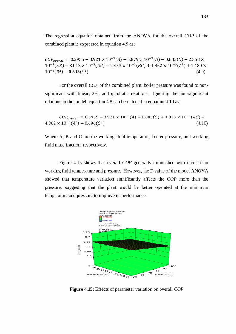
133
The regression equation obtained from the ANOVA for the overall COP of the
combined plant is expressed in equation 4.9 as;
𝐶𝑂𝑃𝑜𝑣𝑒𝑟𝑎𝑙𝑙 = 0.5955 − 3.921 × 10⁻³(𝐴) − 5.879 × 10⁻³(𝐵) + 0.885(𝐶) + 2.358 ×
10−5(𝐴𝐵) + 3.013 × 10⁻³(𝐴𝐶) − 2.453 × 10⁻³(𝐵𝐶) + 4.862 × 10⁻⁶(𝐴2) + 1.480 ×
10−4(𝐵2) − 0.696(𝐶2) (4.9)
For the overall COP of the combined plant, boiler pressure was found to non-
significant with linear, 2FI, and quadratic relations. Ignoring the non-significant
relations in the model, equation 4.8 can be reduced to equation 4.10 as;
𝐶𝑂𝑃𝑜𝑣𝑒𝑟𝑎𝑙𝑙 = 0.5955 − 3.921 × 10⁻³(𝐴) + 0.885(𝐶) + 3.013 × 10⁻³(𝐴𝐶) +
4.862 × 10⁻⁶(𝐴2) − 0.696(𝐶2) (4.10)
Where A, B and C are the working fluid temperature, boiler pressure, and working
fluid mass fraction, respectively.
Figure 4.15 shows that overall COP generally diminished with increase in
working fluid temperature and pressure. However, the F-value of the model ANOVA
showed that temperature variation significantly affects the COP more than the
pressure; suggesting that the plant would be better operated at the minimum
temperature and pressure to improve its performance.
Figure 4.15: Effects of parameter variation on overall COP
Design-Expert® Software
Factor Coding: Actual
COP_overall
0.711296
0.516106
X1 = A: W/F Temp
X2 = B: Boiler Press
Actual Factor
C: W/F C.R = 0.475
12 13
14 15
16 17
18 19
20 21
65 72
79 86
93 100
0.5
0.55
0.6
0.65
0.7
0.75
COP_
over
all
A: W/F Temp (C)B: Boiler Press (Bar)
Design-Expert® Software
Factor Coding: Actual
COP_overall
0.711296
0.516106
X1 = A: W/F Temp
X2 = B: Boiler Press
Actual Factor
C: W/F C.R = 0.475
12 13
14 15
16 17
18 19
20 21
65 72
79 86
93 100
0.5
0.55
0.6
0.65
0.7
0.75
COP_
over
all
A: W/F Temp (C)B: Boiler Press (Bar)

134
4.8 Plant Economic Analysis
The 4th objective of this study is to analyse the economics of the developed
system in comparison with a conventional system of similar cooling capacity, under
the same service conditions.
Economic analysis is carried out not only to assess the financial viability but
also to analyse environmental impact of the project in terms of the emission reduction
in comparison with the selected base case of a same capacity but using different energy
source.
However, since the developed project is less than mini/micro scale, the results
of the analyses may not be impressively significant to conclude on its economic
performance. As such, 3 additional scenarios were analysed under the same operating
conditions so as to observe the developed project in a near practicable sense. The
scenarios analysed with their capacities as; (i) 1.76 kW (or 0.5TR) capacity, (ii) 3.5
kW (or 1TR) capacity, and (iii) 7 kW (or 2TR) capacity.
Analyses of all the four scenarios were carried out based on the projects
financial (internal rate of return, payback time, net present value, and benefit-to-cost
ratio), and environmental (emission analysis) parameters, as contained in Table 4.12
and Table 4.13, respectively. Further details of the techno-economics of the 4
scenarios are contained in appendix H (1-4).
Table 4.12 shows the financial parameters (tax rate, inflation and fuel
escalation rate, project life, and discount rates for each of the considered scenarios.
The inflation rate applies to both the operating and maintenance costs, and the
revenues. An average of RM 2000.00 was used as labour and other inputs costs per
hectare (10,000 m2) of agricultural soil bed per month. Annual vegetable output from
one hectare of land, according to MARDI report by Yahya, was estimated to 18.7 tons
(18,700 kg) (Yahya, 2001), and 1kg of vegetable had been valued at RM 2.5: this is
observed to be reasonably not too optimistic.

135
Table 4.12: Projects financial summary
Economic
Parameter
Items Plant Cooling Capacity
1.76 kW 3.5 kW 7.0 kW
1. Soil bed size (m2) 9.00 18.00 36.00
Fixed Cost (RM) 1. Initial investment 49,350.00 64,525.00 97,650.00
Annual cost (RM)
1. Maintenance &
Repair 350.00 525.00 787.50
2. Labour 21.60 43.20 86.40
3. Tax 0.00 0.00 0.00
Total annual costs (RM) 371.60 568.20 873.90
Annual
Income/Revenue
(RM)
1. Fuel cost saving 3,531.00 7,018.00 13,897.00
2. Electricity export 0.0051 0.0187 0.0505
3. Vegetables sales 60.75 121.50 243.00
Total annual income (RM) 3591.75 7139.52 14140.05
Inflation & Fuel escalation rate (2.5 %) 80.50 164.28 331.65
Expected Annual Cash flow (RM) 3220.15 6571.32 13266.15
IRR 5 % 10 % 14 %
NPV (RM) (1,229.57) 32,902.98 30,607.39
Discount rate 5 % 5 % 10 %
Project life (year) 20 20 20
Payback (year) 12 8 6
Benefits to Cost Ratio 1.34 2.11 1.75
From Table 4.12, the financial viabilities of projects with capacities less than
3.5 kW (1 TR) is observed to be less impressive, considering the NPV and payback
period. This is a laboratory size project which contains nearly all the components of
the bigger capacity sizes; thus, it would be a bit difficult to breakthrough, comparing
the initial cost with the income. Plants with 3.5 kW and 7.0 kW capacities were
observed to be more financially viable with positive NPV, equity payback of 8 years
and 6 years, respectively, and IRR of 10 % and 14 %, respectively. The benefit-to-
cost ratio is better in the 3.5 kW capacity than that of 7.0 kW capacity only because
lower discount rate applied in the former than the later. However, each of the projects
contributed to GHG emission reduction (as shown in Table 4.13), quantified in terms
of the barrels of crude oil not used. The combined yearly cash flows of the projects
over their projected lives in Figure 4.16, also shows that developed project is more
financially viable with bigger capacity.

136
Table 4.13: Projects emission reduction summary
Plant cooling capacity
Net
annual
GHG
emission
reduction
0.05kW 1.76kW 3.5kW 7kW
0.3 tCO2;
Equivalent to
0.7 barrels of
crude oil not
consumed.
11.8 tCO2;
Equivalent to
27.4 Barrels of
crude oil not
consumed.
23.4 tCO2;
Equivalent to
54.4 Barrels of
crude oil not
consumed.
46.4 tCO2;
Equivalent to
108 Barrels of
crude oil not
consumed.
Figure 4.16: Project annual cash flow
4.9 Summary
In this chapter of the thesis, the results had been presented and analysed. The
results presented include the modelling and experimental analyses of the soil cooling,
the chilled water production from absorption chiller, the combined plant and its
parametric analyses, as well as the economic analyses of the developed system for
cooling application.
-150000
-100000
-50000
0
50000
100000
150000
200000
250000
0 1 2 3 4 5 6 7 8 9 10 11 12 13 14 15 16 17 18 19 20Ca
sh F
low
(R
M)
Project Life (year)
1.76 kW 3.5 kW 7.0 kW

137
Analytical models results have been validated with the results obtained from
the experimental setups and good agreements were found between the analyses of the
results obtained from both the experimental rig and the model.
The parametric analyses (through RSM) had been carried out, and the effects
of each of the key parameters had been analysed and discussed for the soil cooling
system, and for combined plant system.
The economic analysis of the combined plant in comparison with a similar
plant for the same application and under the same service condition and environment,
had been studied and discussed. This had shown the viability of the project and its
environmental impacts. The environmental impacts in form of the GHG emission
reduction had also been quantified in terms of the unused barrels of crude oil.
138
CHAPTER 5
5 CONCLUSIONS AND RECOMMENDATIONS
5.1 Conclusion
The energy, in the form of solar heat contained within any given land surface
area, could be harnessed with vapour absorption refrigeration–organic Rankine cycle
(VAR–ORC) combined plant to lower soil temperature. The combined plant makes
use of low-grade solar energy for the production of chilled water in any soil or space
cooling application. However, due to the diffused nature of this source of energy,
solar thermal collector could be installed to capture the required amount of solar energy
to produce a higher rate of chilled water. The cooling load required to lower the soil
temperature could be supplied by an absorption chiller; however, an organic Rankine
cycle would be required to generate the necessary amount of electrical energy to
operate pumps and other ancillary loads of the system.
The cooling load requirement of a particular size of soil bed could only be
optimally offset by a certain capacity of the combined plant. A set of mathematical
models had been successfully developed in this study in order to design a combined
VAR–ORC plant with the right sizing of the required solar thermal collectors for a
given size of a land area. The models would also help in specifying cooling system
requirements as well as the expected system performance.
The physical model developed in this study was suitable for selecting the
chilled water flow rates required to achieve a set of soil temperatures that would be
needed for a particular type of high-value temperate crop. This model had been

139
developed in relation to the soil cooling load, soil bed size and chilled water pipe
dimension; thus, it could be concluded that the application of this physical model could
be extended beyond the experimental size of soil bed in this study with acceptable
range of variations.
The results of the mathematical models in this study had been validated with
those obtained from the experimental rig as presented in Chapter 4, with good
agreement. Variations between the experimental and modelled results were considered
acceptable due to some approximations and simplification assumptions in the models
development. It could be concluded that the developed models could be used to predict
the soil cooling and combined plant performances with reasonable accuracy.
Further analysis of the effects of relevant factors on the performance of the
proposed system using response surface methodology (RSM) showed that chilled water
flow rate had the most significant effect on the temperature of the cooled soil. A
maximum chilled water flow rate of 0.42 kg/min would be sufficient during the peak
load to achieve the set soil temperature (18 ºC ± 2) for 0.25 m2 area of soil bed in this
study.
The effects of the variations in key operating parameters (temperature,
pressure, and working fluid mass fraction) on the combined plant performance showed
that the plant optimum performance would require some trade-offs between the
coefficient of performance and the organic Rankine cycle efficiency. The overall plant
performance diminished at elevated temperature and pressure; thus, operating the plant
at low temperature and pressure would ensure its optimal performance and save the
cost. This is in consonance with the earlier study by (Al-Sulaiman et al., 2012).
The proposed system has higher potential for financial viability with bigger
capacity. As presented in Chapter 4, the economic viability of the proposed system
starts from 3.5 kW capacity upwards. This is based on the financial parameters,
including inflation rate, fuel escalation rates, electricity rate, and selling price of
vegetables.
140
Implementing a project such as in this study has the potential to contribute to
the GHG emission reduction that is equivalent to 6.7 tCO2 per kW of cooling capacity
in a year. It could, therefore, be concluded that the proposed system of soil cooling
would be economically viable and environmentally beneficial.
5.2 Recommendations
This area of study is generally wide in scope and cuts across a number of
technologies and their applications. However, the work reported in this thesis has been
completed within the spate of time and resource, and within the limit of the scope of
this research. As such, the following areas are suggested for future research to gain
more insight into the applications of solar thermal energy for general cooling and
power generation, and for radiant soil or floor cooling systems:
i. Since a complete system, consisting of a large size of soil bed and
bigger capacity of the combined plant, could hardly be explored in a
laboratory and within the stipulated period of this research, any
integration of an absorption chiller with organic Rankine cycle in the
future, for a bigger capacity, for simultaneous cooling and power
generation, would give further insight into the economic viability of the
system;
ii. The study only investigated the sensitivity of soil temperature to the
ambient environment. However, in upgrading the systems to a bigger
size, the dynamic analysis of ambient air and the daytime conditions on
the chilled water plant performance, and its resultant effects on the
cooled soil, should be looked into; and
iii. Since the study had focused only on the agricultural soil cooling, that
is a hydronic radiant cooling system, the application of solar thermal
chilled water from a combined cooling and power could be extended to
a number of radiant cooling systems, including comfort cooling in

141
buildings and other process cooling systems. For such purposes, much
improved programming codes for cooling load and combined plant
capacity estimation should be developed.
142
REFERENCES
Abdulateef., J. M., Sopian., K. and Alghoul, M. A. (2008). Optimum Design for Solar
Absorption Refrigerarion Systems and Comparison of the Performances using
Ammonia-Water, Ammonia-Lithium Nitrate and Ammonia-Sodium
Thiocyanate Solutions. International Journal of Mechanical and Materials
Engineering. 3(1), 17-24.
Abdulateef., J. M., Sopian., K., Alghoul., M. A., Sulaiman., M. Y., Zaharim., A. and
Ahmad, I. (2007). Solar Absorption Refrigeration System Using New Working
Fluid Pairs. International Journal of Energy. 3(1), 1-6.
Abdullah, M. O. and Hieng, T. C. (2010). Comparative analysis of performance and
techno-economics for a H2O–NH3–H2 absorption refrigerator driven by
different energy sources. Applied Energy. 87(5), 1535-1545.
Abed, H., Atashkari, K., Niazmehr, A. and Jamali, A. (2013). Thermodynamic
optimization of combined power and refrigeration cycle using binary organic
working fluid. International Journal of Refrigeration. 36(8), 2160-2168.
Ackom, E. K. (2005). Technical & Economic Viability Analysis of Renewable Energy
Technologies in Ghana. PhD, Brandenburg University of Technology.
Agyenim, F., Knight, I. and Rhodes, M. (2010). Design and experimental testing of
the performance of an outdoor LiBr/H2O solar thermal absorption cooling
system with a cold store. Solar Energy. 84(5), 735-744.
Ahmed, A. and Medhat, A. F. (2012). Tropical Modeling of Concrete-Core-Radiant
Coolingن ystemن “Applicationن onن Alexandria,ن Egypt“.ن 9th International
Conference on Heat Transfer, Fluid Mechanics and Thermodynamics. Malta,
Egypt.
Ahmed, S. F., Amanullah, M. T. O., Khan, M. M. K., Rasul, M. G. and Hassan, N. M.
S. (2016). Parametric study on thermal performance of horizontal earth pipe
cooling system in summer. Energy Conversion and Management. 114, 324-
337.

143
Akbulut.,نU.,نKıncay.,نO.نandنUtlu,نZ.ن.(2016)نAnalysisنofنaنwallنcoolingنsystemنusingن
a heat pump. Renewable Energy. 85, 540-553.
Al-Sulaiman., F. A., Hamdullahpur., F. and Dincer, I. (2012). Performance assessment
of a novel system using parabolic trough solar collectors for combined cooling,
heating, and power production. Renewable Energy. 48, 161-172.
Arvay., P., Muller., M. R., Ramdeen., V. and Cunningham, G. (2011). Economic
Implementation of the Organic Rankine Cycle in Industry. ACEEE Summer
Study on Energy Efficiency in Industry Rutgers University. 1-11.
ASHRAE (2009). Residential cooling and heating load calculations. 2009 American
Society of Heating, Refrigerating and Air-Conditioning Engineers. (pp. 1-16).
ASHRAE.
Ayompe., L. M., Duffy., A., McCormack., S. J. and Conlon, M. (2011). Validated
TRNSYS model for forced circulation solar water heating systems with flat
plate and heat pipe evacuated tube collectors. Applied Thermal Engineering.
31, 1536-1542.
Bajpai, V. K. (2012). Design of Solar Powered Vapour Absorption System.
Proceedings of the World Congress on Engineering WCE 2012 London, U.K.,
1-5.
Baniyounes, A. M., Liu, G., Rasul, M. G. and Khan, M. M. K. (2013). Comparison
study of solar cooling technologies for an institutional building in subtropical
Queensland, Australia. Renewable and Sustainable Energy Reviews. 23, 421-
430.
Bishop., J. and Horspool, R. N. (2008). On the Efficiency of Design Patterns
Implemented in C# 3.0. TOOLS EUROPE. 11, 356-371.
Borunda., M., Jaramillo., O. A., Dorantes., R. and Reyes, A. (2016). Organic Rankine
Cycle coupling with a Parabolic Trough Solar Power Plant for cogeneration
and industrial processes. Renewable Energy. 86, 651-663.
Boyano, A., Hernandez, P. and Wolf, O. (2013). Energy demands and potential savings
in European office buildings: Case studies based on EnergyPlus simulations.
Energy and Buildings. 65, 19-28.
Brenner, A. J., Puigdefa, J., Domingo, F. and Villagarcõ, L. (1999). Evapotranspiration
model for semi-arid shrub-lands tested against data from SE Spain.
Agricultural and Forest Meteorology. 95, 67-84.
144
Cai, D., He, G., Tian, Q. and Tang, W. (2014). Thermodynamic analysis of a novel air-
cooled non-adiabatic absorption refrigeration cycle driven by low grade
energy. Energy Conversion and Management. 86, 537-547.
Carrasco., T. L. and Girty, G. H. (2015). Identifying a reference frame for calculating
mass change during weathering: A review and case study utilizing the C#
program assessing element immobility and critical ratio methodology. Catena.
125, 146-161.
Chang, W. S., Wang, C. C. and Shieh, C. C. (2009). Design and performance of a solar-
powered heating and cooling system using silica gel/water adsorption chiller.
Applied Thermal Engineering. 29(10), 2100-2105.
Chen, Q. and Xu, Y.-C. (2012). An entransy dissipation-based optimization principle
for building central chilled water systems. Energy. 37(1), 571-579.
Chen, W.-n. (2012). Renewable Energy Status in Malaysia. In: Malaysia, S. E. D. A.
(ed.).
Chidambaram, L. A., Ramana, A. S., Kamaraj, G. and Velraj, R. (2011). Review of
solar cooling methods and thermal storage options. Renewable and Sustainable
Energy Reviews. 15(6), 3220-3228.
Chua, S. C. and Oh, T. H. (2012). Solar energy outlook in Malaysia. Renewable and
Sustainable Energy Reviews. 16(1), 564-574.
Cloutier, M. (2002). Refrigeration Cycles. (pp. 1-17).
Cui, P., Yang, H. and Fang, Z. (2008). Numerical analysis and experimental validation
of heat transfer in ground heat exchangers in alternative operation modes.
Energy and Buildings. 40(6), 1060-1066.
Datla, B. V. (2012). Organic Rankine Cycle System Analysis for Low GWP Working
Fluids. International Refrigeration and Air Conditioning Conference. Purdue
University: Purdue e-Pubs.
Daut, I., Zainuddin, F., Irwan, Y. M. and Razliana, A. R. N. (2012). Analysis of Solar
Irradiance and Solar Energy in Perlis, Northern of Peninsular Malaysia. Energy
Procedia. 18, 1421-1427.
De Carli, M. and Tonon, M. (2011). Effect of modelling solar radiation on the cooling
performance of radiant floors. Solar Energy. 85(5), 689-712.
Deam, R. T., Lemma, E., Mace, B. and Collins, R. (2008). On Scaling Down Turbines
to Millimeter Size. Journal of Engineering for Gas Turbines and Power.
130(5), 261-277.

145
Delgado-Torres, A. M. and García-Rodríguez, L. (2010). Analysis and optimization of
the low-temperature solar organic Rankine cycle (ORC). Energy Conversion
and Management. 51(12), 2846-2856.
Demir, H., Koyun, A. and Temir, G. (2009). Heat transfer of horizontal parallel pipe
ground heat exchanger and experimental verification. Applied Thermal
Engineering. 29(2-3), 224-233.
Demirkaya, G., Padilla, R. V. and Goswami, D. Y. (2013). A review of combined
power and cooling cycles. Wiley Interdisciplinary Reviews: Energy and
Environment. 2(5), 534-547.
Deng, J., Wang, R. Z. and Han, G. Y. (2011). A review of thermally activated cooling
technologies for combined cooling, heating and power systems. Progress in
Energy and Combustion Science. 37(2), 172-203.
Dincer, I., Rosen, M. A. and Zamfirescu, C. (2009). Exergetic Performance Analysis
of a Gas Turbine Cycle Integrated With Solid Oxide Fuel Cells. Journal of
Energy Resources Technology. 131(3), 032001.
Dong, B. (2010). Integrated Building Heating, Cooling and Ventilation Control. PhD,
Carnegie Mellon University.
Duan, Z., Zhan, C., Zhang, X., Mustafa, M., Zhao, X., Alimohammadisagvand, B. and
Hasan, A. (2012). Indirect evaporative cooling: Past, present and future
potentials. Renewable and Sustainable Energy Reviews. 16(9), 6823-6850.
Duggirala, B. (2010). Analyzing Sustainable Energy Opportunities for a Small Scale
Off-Grid Facility: A Case Study at Experimental Lakes Area (ELA), Ontario.
Master, University of Manitoba.
Feng, X., Goswami., D. Y. and Bhagwat, S. S. (2000). A combined power/cooling
cycle. Energy. 25, 233-246.
Flueckiger, S. M., Yang, Z. and Garimella, S. V. (2013). Review of Molten-Salt
Thermocline Tank Modeling for Solar Thermal Energy Storage. Heat Transfer
Engineering. 34(10), 787-800.
Fong, K. F., Chow, T. T., Lee, C. K., Lin, Z. and Chan, L. S. (2009). Comparative
study of different solar cooling systems for buildings in subtropical city. Solar
Energy. 84(2), 227-244.
Fong, K. F., Chow, T. T., Lee, C. K., Lin, Z. and Chan, L. S. (2010a). Advancement
of solar desiccant cooling system for building use in subtropical Hong Kong.
Energy and Buildings. 42(12), 2386-2399.
146
Fong, K. F., Lee, C. K., Chow, T. T., Lin, Z. and Chan, L. S. (2010b). Solar hybrid air-
conditioning system for high temperature cooling in subtropical city.
Renewable Energy. 35(11), 2439-2451.
Freund, S. W. 2012. Rankine Cycle Integrated with Absorption Chiller. NY, United
States patent application 12/916,191.
Gaglia, A. G., Lykoudis, S., Argiriou, A. A., Balaras, C. A. and Dialynas, E. (2017).
Energy efficiency of PV panels under real outdoor conditions–An experimental
assessment in Athens, Greece. Renewable Energy. 101, 236-243.
Garimella, S. (2012). Low-grade waste heat recovery for simultaneous chilled and hot
water generation. Applied Thermal Engineering. 42, 191-198.
Gastli, A. and Charabi, Y. (2011). Solar water heating initiative in Oman energy saving
and carbon credits. Renewable and Sustainable Energy Reviews. 15(4), 1851-
1856.
Gontard, N., Guilbert, S. and Cuq, J.-L. (1992). Edible Wheat Gluten Films: Influence
of the Main Process Variables on Film Properties using Response Surface
Methodology. Journal of Food Science. 57(1), 190-199.
Gordon, J. M. and Ng, K. C. (1995). A General Thermodynamic Model for Absorption
Chillers: Theory and Experiment. Heat Recovery Systems & CHP. 15(1), 73-
83.
Gorman, J. M., Sparrow, E. M. and Abraham, J. P. (2013). Differences between
measured pipe wall surface temperatures and internal fluid temperatures. Case
Studies in Thermal Engineering. 1(1), 13-16.
Goswami, D. Y. and Xu, F. (1999). Analysis of a New Thermodynamic Cycle for
Combined Power and Cooling Using Low and Mid Temperature Solar
Collectors Journal of Solar Energy Engineering. 121, 91-97.
Gupta, Y. (2011). Research and Development of a Small - Scale Adsorption Cooling
System. PhD, Arizona State University.
Hamid, F., Akhbar, S. and Halim, K. H. K. (2013). Mechanical and Thermal Properties
of Polyamide 6/HDPE-g- MAH/High Density Polyethylene. Procedia
Engineering. 68, 418-424.
Han, X. and Zhang, X. (2011). Experimental study on a residential temperature–
humidity separate control air-conditioner. Energy and Buildings. 43(12), 3584-
3591.

147
Hariharan, N. M., Sivashanmugam, P. and Kasthurirengan, S. (2013). Optimization of
thermoacoustic refrigerator using response surface methodo- logy*. Journal of
Hydynamics. 25(1), 72-82.
Hasson, A. M. and Hussain, R. (1987). Effect of Polyethylene Mulch on Soil
Temperature Variation under Planted Greenhouse in Aridic Region. Solar &
Wind Technology. 4(4), 459-465.
He, T., Zhang, X., Wang, C., Wang, M., Li, B., Xue, N., Shimizu, K., Takahashi, K.
and Wu, Y. (2015). Application of Solar Thermal Cooling System Driven by
Low Temperature Heat Source in China. Energy Procedia. 70, 454-461.
He, Z., Zhao, Z., Zhang, X. and Feng, H. (2010). Thermodynamic properties of new
heat pump working pairs: 1,3-Dimethylimidazolium dimethylphosphate and
water, ethanol and methanol. Fluid Phase Equilibria. 298(1), 83-91.
Hlbauer, W. M. I. (1986). Performance of solar crop dryers. 5, 121-137.
Ho-Yan, B. P. (2011). Tesla Turbine for Pico Hydro Applications. Guelph Engineering
Journal. 4, 1-8.
Hong, D., Chen, G., Tang, L. and He, Y. (2011). A novel ejector-absorption combined
refrigeration cycle. International Journal of Refrigeration. 34(7), 1596-1603.
Hoya, G. A. and Guha, A. (2009). The design of a test rig and study of the performance
and efficiency of a Tesla disc turbine. Proceedings of the Institution of
Mechanical Engineers. Part A: Journal of Power and Energy, 451-465.
Hubbard, R. S. (2011). Energy Impacts of Chilled-Water-Piping Configuration. In:
Inc, J. C. (ed.). HPAC Engineering.
Huntingford, C., Verhoef, A., Stewart, J. and Huntingfors, C. (2000). Dual versus
single source models for estiamting surface temperature of African Savannah.
Hydrology and Earth System Sciences. 4(1), 185–191.
Ibrahim, N. I., Al-Sulaiman, F. A. and Ani, F. N. (2017). Solar absorption systems
with integrated absorption energy storage–A review. Renewable and
Sustainable Energy Reviews. Article in press, 10.
Ilenikhena, P. A. and Ezemonye, L. N. (2010). Solar Energy Applications in Nigeria.
WEC MONTREAL.
INEOS Typical Engineering Properties of High Density Polyethylene. In: Polymers,
I. O. (ed.). USA: INEOS Olefins & Polymers.
Jaafar, A. B. (2014). Ocean Thermal Energy-driven Development in Malaysia. Ocean
Thermal Energy Conversion Center, Universiti Teknologi Malaysia.
148
Jain., D. and Tiwari, G. N. (2002). Modeling and optimal design of evaporative cooling
system in controlled environment greenhouse. Energy Conversion and
Management. 43, 2235-2250.
Javidmand, P. and Hoffmann, K. A. (2016). A comprehensive modeling of choked
two-phase flow through short-tube orifices with application to alternative
refrigerants HFO-1234yf and HFO-1234ze. International Journal of
Refrigeration. 69, 114-135.
Jiangfeng, W., Dai, Y., Gao, L. and Ma, S. (2009). A new combined cooling, heating
and power system driven by solar energy. Renewable Energy. 34(12), 2780-
2788.
Jim, F. P. G. and Charles, D. J. (2009). Tropical agriculture. The weather and climate
of the tropics. (pp. 6). Royal Meteorological Society: Royal Meteorological
Society.
Kadir, M. Z. A. A. and Rafeeu, Y. (2010). A review on factors for maximizing solar
fraction under wet climate environment in Malaysia. Renewable and
Sustainable Energy Reviews. 14(8), 2243-2248.
Kalina, A. I. (1984). Combined-Cycle System With Novel Bottoming Cycle. Journal
of Engineering for Gas Turbines and Power. 106, 737-742.
Kalkan, N., Young, E. A. and Celiktas, A. (2012). Solar thermal air conditioning
technology reducing the footprint of solar thermal air conditioning. Renewable
and Sustainable Energy Reviews. 16(8), 6352-6383.
Kalogirou, S. A. (2004). Solar thermal collectors and applications. Progress in Energy
and Combustion Science. 30(3), 231-295.
Kalogirou., S., Florides., G., Tassou., S. and Wrobel, L. (2001). Design and
Construction of a Lithium Bromide Water Absorption Refrigerator. CLIMA
2000/Napoli 2001 World Congress. Napoli: CLIMA.
Karellas., S. and Schuster, A. (2008). Supercritical Fluid Parameters in Organic
Rankine Cycle Applications. International Journal of Thermodynamics. 11(3),
101-108.
Kasperski, J. and Eichler, J. (2012). Ammonia–water absorption cycle on three-
dimensional graphs – The Absorption 3D tool software. International Journal
of Refrigeration. 35(7), 1958-1966.
Kaushik, S. C., Tomar, C. S. and Chandra, S. (1983). Coefficient of Performance of an
Ideal Absorption Cycle. Applied Energy. 14, 115-121.

149
Kaygusuz, K. (2012). Energy for sustainable development: A case of developing
countries. Renewable and Sustainable Energy Reviews. 16(2), 1116-1126.
Khamooshi, M., Parham, K. and Atikol, U. (2013). Overview of Ionic Liquids Used as
Working Fluids in Absorption Cycles. Advances in Mechanical Engineering.
2013, 1-7.
Khan, H. A. and Pervaiz, S. (2013). Technological review on solar PV in Pakistan:
Scope, practices and recommendations for optimized system design.
Renewable and Sustainable Energy Reviews. 23, 147-154.
Khan, M. M. A., Ibrahim, N. I., Saidur, R., Mahbubul, I. M. and Al-Sulaiman, F. A.
(2016). Performance assessment of a solar powered ammonia–water absorption
refrigeration system with storage units. Energy Conversion and Management.
126, 316-328.
Khennich, M. and Galanis, N. (2012). Optimal Design of ORC Systems with a Low-
Temperature Heat Source. Entropy. 14(12), 370-389.
Kim, Y. J., Kim, S., Joshi, Y. K., Fedorov, A. G. and Kohl, P. A. (2012).
Thermodynamic analysis of an absorption refrigeration system with ionic-
liquid/refrigerant mixture as a working fluid. Energy. 44(1), 1005-1016.
KumeGuide (2014). Deep Sea Water Research Institute.
Kusuda, T. and Archenbach, P. R. (1965). Earth temperature and thermal diffusivity
at selected stations in the United States. ASHRAE Transaction. 71(1), 61-75.
Labeke., M.-C. v. and Dambre, P. (1993). Response of five Alstroemeria cultivars to
soil cooling and supplementary lighting. Scientia Horticulturae. 56, 135-145.
Leavell, K. A. B. (2010). Practical Solar Thermal Chilled Water. Proceedings from the
Thirty-second Industrial Energy Technology Conference New Orleans, Los
Angeles. ESL-IE-10-05-03, 1-15.
Lee, J.-Y., Chen, C.-L., Wen, T.-L., Ng, D. K. S., Foo, D. C. Y. and Wang, T.-C.
(2013). Synthesis and design of chilled water networks using mathematical
optimization. Applied Thermal Engineering. 58(1-2), 638-649.
Lee, K.-H., Lee, D.-W., Baek, N.-C., Kwon, H.-M. and Lee, C.-J. (2012). Preliminary
determination of optimal size for renewable energy resources in buildings
using RETScreen. Energy. 47(1), 83-96.
Lee, K. H. and Strand, R. K. (2008). The cooling and heating potential of an earth tube
system in buildings. Energy and Buildings. 40(4), 486-494.

150
Lee., K. H. and Strand, R. K. (2006). Implementation of an Earth tube System into
Energyplus Program. In: Illinois, U. o. (ed.).
Leslie., N. P., Sweetser., R. S., Stovall., T. K. and Zimron, O. (2009). Recovered
Energy Generation Using an Organic Rankine Cycle System. In: ASHRAE
(ed.).
Li, H., Bu, X., Wang, L., Long, Z. and Lian, Y. (2013). Hydrocarbon working fluids
for a Rankine cycle powered vapor compression refrigeration system using
low-grade thermal energy. Energy and Buildings. 65, 167-172.
Liu, B. C., Liu, W. and Peng, S. W. (2005). Study of heat and moisture transfer in soil
with a dry surface layer. international Journal of Heat and Mass Transfer. 48,
4579-4589.
Liu, S., Lu, L., Mao, D. and Jia, L. (2007). Evaluating parameterizations of
aerodynamic resistance to heat transfer using field measurements. Hydrology
and Earth System Sciences. 11(1), 769-783.
Liu, X.-f., Liu, J.-p., Lu, J.-d., Liu, L. and Zou, W. (2012). Research on operating
characteristics of direct-return chilled water system controlled by variable
temperature difference. Energy. 40(1), 236-249.
Liu, X., Zhang, Y., Shen, J., Yao, S. and Zhang, Z. (2016). Characteristics of air
cooling for cold storage and power recovery of compressed air energy storage
(CAES) with inter-cooling. Applied Thermal Engineering. 107, 1-9.
Liu., M., Saman., W. and Bruno, F. (2014). Computer simulation with TRNSYS for a
mobile refrigeration system incorporating a phase change thermal storage unit.
Applied Energy. 132, 226-235.
Lu, Z. S., Wang, R. Z., Xia, Z. Z., Lu, X. R., Yang, C. B., Ma, Y. C. and Ma, G. B.
(2013). Study of a novel solar adsorption cooling system and a solar absorption
cooling system with new CPC collectors. Renewable Energy. 50, 299-306.
Lu., S. and Goswami, D. Y. (2002). Theoretical Analysis of Ammonia-Based
Combined Power/Refrigeration Cycle at Low Refrigeration Temperatures.
International Solar Energy Conference Reno, Nevada, USA. ASME, 117-125.
Luzzi, A., Lovegrove., K., Filippi., E., Fricker., H., Schmitz-Goeb., M., Chandapillai.,
M. and Kaneff, S. (1999). Techno-Economic Analysis of a 10 Mwe Solar
Thermal Power Plant using Ammonia-Based Thermochemical Energy Storage.
Solar Energy. 66(2), 91-101.

151
Lychnos, G. and Davies, P. A. (2012). Modelling and experimental verification of a
solar-powered liquid desiccant cooling system for greenhouse food production
in hot climates. Energy. 40(1), 116-130.
Mansouri Majoumerd, M. and Assadi, M. (2014). Techno-economic assessment of
fossil fuel power plants with CO2 capture – Results of EU H2-IGCC project.
International Journal of Hydrogen Energy. 39(30), 16771-16784.
Maraver, D., Sin, A., Royo, J. and Sebastián, F. (2013). Assessment of CCHP systems
based on biomass combustion for small-scale applications through a review of
the technology and analysis of energy efficiency parameters. Applied Energy.
102, 1303-1313.
Marc, O., Sinama, F. and Lucas, F. (2012). Decision making tool to design solar
cooling system coupled with building under tropical climate. Energy and
Buildings. 49, 28-36.
MARDI. Malaysian Agriculture Research and Development Institute.
Marı,ن E. G., Colomer, R. P. G. and Blaise-Ombrecht, C. A. (2007). Performance
analysis of a solar still integrated in a greenhouse. Desalination. 203(1-3), 435-
443.
Martínez, P. J., Martínez, J. C. and Lucas, M. (2012). Design and test results of a low-
capacity solar cooling system in Alicante (Spain). Solar Energy. 86(10), 2950-
2960.
Massaguer., E., Massaguer., A., Montoro., L. and Gonzalez, J. R. (2014). Development
and validation of a new TRNSYS type for the simulation of thermoelectric
generators. Applied Energy. 134, 65-74.
Masson., S. V., Qu., M. and H.Archer, D. (2006). Performance Modeling of a Solar
Drivenن Absorptionن Coolingن ystemن forن Carnegieن Mellonن University’sن
Intelligent Workplace. ICEBO2006, Shenzhen, China. China: Renewable
Energy Resources and a Greener Future.
Max, J. F. J., Horst, W. J., Mutwiwa, U. N. and Tantau, H.-J. (2009). Effects of
greenhouse cooling method on growth, fruit yield and quality of tomato
(Solanum lycopersicum L.) in a tropical climate. Scientia Horticulturae.
122(2), 179-186.
Mazouz, S., Mansouri, R. and Bellagi, A. (2014). Experimental and thermodynamic
investigation of an ammonia/water diffusion absorption machine. International
Journal of Refrigeration. 45, 83-91.

152
McQuay (2001). Chiller Plant Design. In: International, M. (ed.). McQuay
International.
McQuay (2002). Application Guide: Refrigerants. In: International, M. (ed.). McQuay
International.
Mekhilef, S., Faramarzi, S. Z., Saidur, R. and Salam, Z. (2013). The application of
solar technologies for sustainable development of agricultural sector.
Renewable and Sustainable Energy Reviews. 18, 583-594.
Mekhilef, S., Safari, A., Mustaffa, W. E. S., Saidur, R., Omar, R. and Younis, M. A.
A. (2012). Solar energy in Malaysia: Current state and prospects. Renewable
and Sustainable Energy Reviews. 16(1), 386-396.
Mendonça, M., Lacey, S. and Hvelplund, F. (2009). Stability, participation and
transparency in renewable energy policy: Lessons from Denmark and the
United States. Policy and Society. 27(4), 379-398.
Mihalakakou, G. (2002). On estimating soil surface temperature profiles. Energy and
Buildings. 34, 251-259.
Mikeska., T. and Svendsen, S. (2015). Dynamic behavior of radiant cooling system
based on capillary tubes in walls made of high performance concrete. Energy
and Buildings. 108, 92-100.
Miles, D. J., Sannors, D. M., Nowakowski, G. A. and Shelton, S. V. (1993). Gas Fired
Sorption Heat Pump Development. Heat Recovery Systems & CHP. 13(4), 347-
351.
Miyazaki, T. and Akisawa, A. (2009). The influence of heat exchanger parameters on
the optimum cycle time of adsorption chillers. Applied Thermal Engineering.
29(13), 2708-2717.
Mokhtar, M., Ali, M. T., Bräuniger, S., Afshari, A., Sgouridis, S., Armstrong, P. and
Chiesa, M. (2010). Systematic comprehensive techno-economic assessment of
solar cooling technologies using location-specific climate data. Applied
Energy. 87(12), 3766-3778.
Moncef, K. and Kreider, J. F. (1996). Analytical Model for Heat Transfer in an
Underground Air Tunnel. Energy Conversion Management. 17(10), 1561-
1574.
Mongkon, S., Thepa, S., Namprakai, P. and Pratinthong, N. (2013). Cooling
performance and condensation evaluation of horizontal earth tube system for
the tropical greenhouse. Energy and Buildings. 66, 104-111.

153
Mongkon, S., Thepa, S., Namprakai, P. and Pratinthong, N. (2014). Cooling
performance assessment of horizontal earth tube system and effect on planting
in tropical greenhouse. Energy Conversion and Management. 78, 225-236.
Morille, B., Migeon, C. and Bournet, P. E. (2013). Is the Penman–Monteith model
adapted to predict crop transpiration under greenhouse conditions? Application
to a New Guinea Impatiens crop. Scientia Horticulturae. 152, 80-91.
Moser, A. P. and Folkman, S. (2008). Buried Pipe Design. Third Edition. edition. New
York, Chicago, San Francisco, Lisbon, London, Madrid, Mexico City, Milan,
New Delhi, San Juan, Seoul, Singapore, Sydney, Toronto: Mc Graw Hill.
Muerth, M. and Mauser, W. (2012). Environmental Modelling & Software Rigorous
evaluation of a soil heat transfer model for mesoscale climate change impact
studies. Environmental Modelling and Software. 35, 149-162.
Munson., B. R., Young., D. F., Okiishi., T. H. and Huebsch, W. W. (2009).
Fundamentals of Fluid Mechanics. United States of America: John Wiley &
Sons, Inc.
Nabi, G. and Mullins, C. E. (2008). Soil Temperature Dependent Growth of Cotton
Seedlings Before Emergence. Pedosphere. 18(1), 54-59.
NASA , National Aeronautic and Space Administration. Global Energy Budget.
Accessed 2017. Cited 2017
Neckel, A. L. and Godinho, M. (2015). nfluence of geometry on the efficiency of
convergent–divergent nozzles applied to Tesla turbines. Experimental Thermal
and Fluid Science. 62, 131-140.
Nik., A. R., Kasran., B. and Hassan, A. (1986). Soil Temperature Regimes under
Mixed Dipterocarp Forests of Peninsular Malaysia. Pertanika. 9(3), 277-284.
NIST, N. I. o. S. a. T. Reference Fluid Thermodynamic and Transport Properties -
REFPROP. U.S Department of Commerce.
Niu, F., Yu, Y., Yu, D. and Li, H. (2015). Heat and mass transfer performance analysis
and cooling capacity prediction of earth to air heat exchanger. Applied Energy.
137, 211-221.
Nizami, D. J., Lightstone, M. F., Harrison, S. J. and Cruickshank, C. A. (2013).
Negative buoyant plume model for solar domestic hot water tank systems
incorporating a vertical inlet. Solar Energy. 87, 53-63.
Nordin., N. A. M., Zaharudin., Z. A., Maasar., M. A. and Nordin, N. A. (2012). Finding
Shortest Path of the Ambulance Routing: Interface of A* Algorithm using C#

154
Programming. IEEE Symposium on Humanities, Science and Engineering
Researc. Malaysia.
Novak, M. D. (1981). The Moisture and Thermal Regimes od a Bare Soil in the Lower
Fraser Valley During Spring. PhD, The University of British Columbia.
Novak, M. D. (2010). Dynamics of the near-surface evaporation zone and
corresponding effects on the surface energy balance of a drying bare soil.
Agricultural and Forest Meteorology. 150(10), 1358-1365.
Oh, T. H., Pang, S. Y. and Chua, S. C. (2010). Energy policy and alternative energy in
Malaysia: Issues and challenges for sustainable growth. Renewable and
Sustainable Energy Reviews. 14(4), 1241-1252.
Olesen, B. (2008). Radiant Floor Cooling Systems. ASHRAE Journal. 50(9), 16-22.
Olesen, B. W. (1997). Possibilities and limitations of radiant floor cooling.
Othman, N. F., Ya'acob, M. E., Abdul-Rahim, A. S., Othman, M. S., Radzi, M. A. M.,
Hizam, H., Wang, Y. D., Ya'acob, A. M. and Jaafar, H. Z. E. (2015). Embracing
new agriculture commodity through integration of Java Tea as high Value
Herbal crops in solar PV farms. journal of Cleaner Production. 91, 71-77.
Padilla, R. V., Demirkaya, G., Goswami, D. Y., Stefanakos, E. and Rahman, M. M.
(2010). Analysis of power and cooling cogeneration using ammonia-water
mixture. Energy. 35(12), 4649-4657.
Parameshwaran, R., Kalaiselvam, S., Harikrishnan, S. and Elayaperumal, A. (2012).
Sustainable thermal energy storage technologies for buildings: A review.
Renewable and Sustainable Energy Reviews. 16(5), 2394-2433.
Park., K. A., Choi., Y. M., Choi., H. M., Cha., T. S. and Yoon, B. H. (2001). The
evaluation of critical pressure ratios of sonic nozzles at low Reynolds numbers.
Flow Measurement and Instrumentation. 12, 37-41.
Peet, M., Sato, S., Clément, C. and Pressman, E. (2003). Heat Stress Increases
Sensitivity of Pollen, Fruit and Seed Production in Tomatoes (Lycopersicon
Esculentum Mill.) to Non-Optimal Vapor Pressure Deficits. Acta Hortic. 618,
209-215.
Pratihar, A. K., Kaushik, S. C. and Agarwal, R. S. (2010). Simulation of an ammonia–
water compression–absorption refrigeration system for water chilling
application. International Journal of Refrigeration. 33(7), 1386-1394.
155
Price,نH.,نLupfert,نE.,نKearney,نD.,نZarza,نE.,نCohen,نG.,نGee,نR.نandنMahoney,نR.ن
(2002). Advances in Parabolic Trough Solar Power Technology. Journal of
Solar Energy Engineering. 124(2), 109.
Puri, S., Beg, Q. K. and Gupta, R. (2002). Optimization of Alkaline Protease
Production from Bacillus sp. by Response Surface Methodology. Current
Microbiology. 44, 286-290.
Puri, V. M. (1987). Heat and Mass Transfer Analysis and Modeling in Unsaturated
Ground Soils for Buried Tube Systems. Energy in Agriculture. 6, 179-193.
Qela., B. and Mouftah, H. (2008). Simulation of a House Heating System using C# -
an Energy Conservation Perspective. In: University of Ottawa, O., ON Canada
(ed.). School of Information Technology and Engineering, University of
Ottawa, Ottawa, ON Canada.
Qin, Z., Berliner, P. and Karnieli, A. (2002). Numerical solution of a complete surface
energy balance model for simulation of heat fluxes and surface temperature
under bare soil environment. Applied Mathematics and Computation. 130(1),
171-200.
Qu, M. (2008). Model Based Design and Performance Analysis of Solar Absorption
Cooling and Heating System. PhD, Carnegie Mellon University.
Qu, M., Yin, H. and Archer, D. H. (2010). A solar thermal cooling and heating system
for a building: Experimental and model based performance analysis and design.
Solar Energy. 84(2), 166-182.
Quoilin, S., Broek, M. V. D., Declaye, S., Dewallef, P. and Lemort, V. (2013). Techno-
economic survey of Organic Rankine Cycle (ORC) systems. Renewable and
Sustainable Energy Reviews. 22, 168-186.
Quoilin., S. and Lemort, V. (2009). Technological and Economical Survey of Organic
Rankine Cycle Systems. 5th Eyropean Conference on Economics and
Management of Energy Industry. Algarve, Portugal.
Ramos, M. C. and Martínez-Casasnovas, J. A. (2010). Effects of precipitation patterns
and temperature trends on soil water available for vineyards in a Mediterranean
climate area. Agricultural Water Management. 97(10), 1495-1505.
Rasih, R. A. and Ani, F. N. (2012). Double-Effect Solar Absorption Thermal Energy
Storage. Jurnal Mekanikal. (35), 38-53.

156
RETScreen (2005). RETScreen® software. 2007 ed. RETScreen International Clean
Energy Decision Support Centre: RETScreen International Clean Energy
Decision Support Centre.
Rice, W. (1965). An Analytical and Experimental Investigation of Multiple-Disk
Turbines Journal of Engineering for Power. 29-33.
Romanin, V. D. (2012). Theory and Performance of Tesla Turbines. PhD, University
of California, Berkeley.
Rong, L., Hou, X., Jia, Z., Han, Q., Ren, X. and Yang, B. (2013). Effects on soil
temperature, moisture, and maize yield of cultivation with ridge and furrow
mulching in the rainfed area of the Loess Plateau, China. Agricultural Water
Management. 116, 101-109.
Rose, C. W. (1969). Agricultural Physics. 2nd. edition. Oxford, London, Edinburgh,
New York, Toronto, Sydney, Paris, Braunschweig: Pergamon Press, Oxford.
Rout, S. K., Choudhury, B. K., Sahoo, R. K. and Sarangi, S. K. (2014). Multi-objective
parametric optimization of Inertance type pulse tube refrigerator using
response surface methodology and non-dominated sorting genetic algorithm.
Cryogenics. 62, 71-83.
Sabetia., V. and Boyaghchi, F. A. (2016). Multi-objective Optimization of a Solar
Driven Combined Power and Refrigeration System Using Two Evolutionary
Algorithms Based on Exergoeconomic Concept. Journal of Renewable Energy
and Environment. 3(1), 43-51.
Safa., A. A., Fung., A. S. and Kumar, R. (2015). Heating and cooling performance
characterisation of ground source heat pump system by testing and TRNSYS
simulation. Renewable Energy. 84, 565-575.
Said, S. A. M., El-Shaarawi, M. A. I. and Siddiqui, M. U. (2012). Alternative designs
for a 24-h operating solar-powered absorption refrigeration technology.
International Journal of Refrigeration. 35(7), 1967-1977.
Saitoh, T., Yamada, N. and Wakashima, S.-i. (2007). Solar Rankine Cycle System
Using Scroll Expander. Journal of Environment and Engineering. 2(4), 708-
719.
Sakellari, D. (2005). Modelling the Dynamics of Domestic Low-Temperature Heat
Pump Heating Systems for Improved Performance and Thermal Comfort - A
Systems Approach. Doctor of Philosophy Thesis, Royal Institute of Technology
Stockholm, Sweden.
157
Sanaye, S. and Sarrafi, A. (2015). Optimization of combined cooling, heating and
power generation by a solar system. Renewable Energy. 80, 699-712.
Sanjay, V. (2003). Thermodynamics Studies on Alternative Binary Working Fluids
Combinations and Configurations for a Combined Power and Cooling Cycle.
University of Florida.
Sattelmacher, B., Marschner, H. and Kuhne, R. (1990). Effects of Root Zone
Temperature on Root Activity of Two Potato {Sohnum tuberosum L.) Clones
with Different Adaptation to High Temperature. Journal of Agronnomy and
Crop Science. 165, 131-137.
Schimpf, S. and Span, R. (2015). Simulation of a solar assisted combined heat pump
– Organic rankine cycle system. Energy Conversion and Management. 102,
151-160.
Schröder, E., Neumaier, K., Nagel, F. and Vetter, C. (2014). Study on Heat Transfer
in Heat Exchangers for a New Supercritical Organic Rankine Cycle. Heat
Transfer Engineering. 35(18), 1505-1519.
Seo., J.-M., Song., D. and Lee, K. H. (2014). Possibility of coupling outdoor air cooling
and radiant floor cooling under hot and humid climate conditions. Energy and
Buildings. 81, 219-226.
Sharizal, S. A. (2006). Integrated Solar Energy and Absorption Cooling Model for
HVAC (Heating, Ventilating, and Air Onditioning) Applications in Buildings.
PhD, Michigan Technological University.
Shuttleworth, W. J. and Wallace, J. S. (1985). Evaporation from sparse crops-an
energy combination theory. Quarterly Journal of the Royal Meteorological
Society. 111(469), 839-855.
Siegenthaler, J. 2014. Hydronic Radiant Ceiling Cooling for Smaller Buildings.
Hydronics Zones, p.22.
Smith, A. D., Mago, P. J. and Fumo, N. (2013). Benefits of thermal energy storage
option combined with CHP system for different commercial building types.
Sustainable Energy Technologies and Assessments. 1, 3-12.
Solangi, K. H., Islam, M. R., Saidur, R., Rahim, N. A. and Fayaz, H. (2011). A review
on global solar energy policy. Renewable and Sustainable Energy Reviews.
15(4), 2149-2163.

158
Somers, C., Mortazavi, A., Hwang, Y., Radermacher, R., Rodgers, P. and Al-Hashimi,
S. (2011). Modeling water/lithium bromide absorption chillers in ASPEN Plus.
Applied Energy. 88(11), 4197-4205.
Sotomonte., C. A. R., Ribeiro., S., Oliveira., E., Lora., E. E. S. and Venturini, O. J.
(2011). Organic Rankine Cycle Associated with an Absorption Chiller for
Biomass Applications. Engenharia Térmica. 10(01-02), 11-22.
özen,نA.,نMenlik,نT.نandنÖzbaş,نE.ن.(2012)نTheنeffectنofنejectorنonنtheنperformanceن
of diffusion absorption refrigeration systems: An experimental study. Applied
Thermal Engineering. 33-34, 44-53.
Srikhirin., P., Aphornratana., S. and Chungpaibulpatana, S. (2001). A review of
absorption refrigeration technologies. Renewable and Sustainable Energy
Reviews. 5, 343-372.
Ssembatya., M., Pokhrel., M. K. and Reddy, R. (2014). Simulation studies on
performance of solar cooling system in UAE conditions. Energy Procedia. 48,
1007-1016.
Stanish, M. A. and Perlmutter, D. D. (1981). Salt Hydrates as Absorbents in Heat Pump
Cycles. Solar Energy. 26, 333-339.
Stevanovic, S. (2016). Parametric study of a cost-optimal, energy efficient office
building in Serbia. Energy. 117(2016), 492-505.
Stodola, N. and Modi, V. (2009). Penetration of solar power without storage. Energy
Policy. 37(11), 4730-4736.
Subramanian, R. S. (2008). Heat transfer in Flow Through Conduits. In: University,
D. o. C. a. B. E. C. (ed.) Department of Chemical and Biomolecular
Engineering Clarkson University.
Sukri, M. F., Musa, M. N., Senawi, M. Y. and Nasution, H. (2016). Modeling and
Parametric Study of Cooling Loads Characteristics for Automotive
AirConditioning System. Applied Mechanics & Materials. 819, 189-201.
Tamm, G., Goswami, D. Y., Lu, S. and Hasan, A. A. (2004). Theoretical and
experimental investigation of an ammonia–water power and refrigeration
thermodynamic cycle. Solar Energy. 76(1-3), 217-228.
Tamm, G. O. (2003). Experimental Investigation of an Ammonia-Based Combined
Power and Cooling Cycle. PhD, University of Florida.
Tang, C. K. (2012). Chapter 2 – Malaysia’sنWeatherنData.نBuilding Energy Efficiency
Technical Guideline for Passive Design. (pp. 1-30). Malaysia.
159
Tarigan, E., Djuwari and Kartikasari, F. D. (2015). Techno-economic Simulation of a
Grid-connected PV System Design as Specifically Applied to Residential in
Surabaya, Indonesia. Energy Procedia. 65, 90-99.
Tchanche, B. F., Lambrinos, G., Frangoudakis, A. and Papadakis, G. (2011). Low-
grade heat conversion into power using organic Rankine cycles – A review of
various applications. Renewable and Sustainable Energy Reviews. 15(8), 3963-
3979.
Tetëns, O. (1930). Über einige meteorologische begriffe. Z. Geophys. 6, 297–309.
Thongtip, T. and Aphornratana, S. (2017). An experimental analysis of the impact of
primary nozzle geometries on the ejector performance used in R141b ejector
refrigerator. Applied Thermal Engineering. 110, 89-101.
Tozer, R., Syed, A. and Maidment, G. (2005). Extended temperature–entropy (T–s)
diagrams for aqueous lithium bromide absorption refrigeration cycles.
International Journal of Refrigeration. 28(5), 689-697.
Treberspurg., M., Djalili., M., Staller., B. H. and IFZ (2011). New technical solutions
for energy efficient buildings. In: SCI-Network (ed.).
Tsoutsos., T., Karagiorgas., M., Zidianakis., G., Drosou., V., Aidonis., A., Gouskos.,
Z. and Moeses, C. (2009). Development of the Application of Solar Thermal
Cooling Systems in Greece and Cyprus. Fresenius Environmental Bulletin.
8(7b), 1-15.
Ullah, K. R., Saidur, R., Ping, H. W., Akikur, R. K. and Shuvo, N. H. (2013). A review
of solar thermal refrigeration and cooling methods. Renewable and Sustainable
Energy Reviews. 24, 499-513.
Vadiee, A. and Martin, V. (2013). Thermal energy storage strategies for effective
closed greenhouse design. Applied Energy. 109, 337-343.
Vijayaraghavan, S. and Goswami, D. Y. (2003). On Evaluating Efficiency of a
Combined Power and Cooling Cycle. Journal of Energy Resources
Technology. 125(3), 221.
Villagarcía, L., Were, A., Domingo, F., García, M. and Alados-Arboledas, L. (2007).
Estimation of soil boundary-layer resistance in sparse semiarid stands for
evapotranspiration modelling. Journal of Hydrology. 342(1-2), 173-183.
Wang, H., Peterson, R. and Herron, T. (2011). Design study of configurations on
system COP for a combined ORC (organic Rankine cycle) and VCC (vapor
compression cycle). Energy. 36(8), 4809-4820.
160
Wang, J., Wang, J., Zhao, P. and Dai, Y. (2016). Thermodynamic analysis of a new
combined cooling and power system using ammonia–water mixture. Energy
Conversion and Management. 117, 335-342.
Wang, R. Z., Ge, T. S., Chen, C. J., Ma, Q. and Xiong, Z. Q. (2009). Solar sorption
cooling systems for residential applications: Options and guidelines.
International Journal of Refrigeration. 32(4), 638-660.
Wattanakit., S., Chirarattananon., S. and Chaiwiwatworakul, P. (2014). Comfort
Assessment of Radiant Cooling in Building in Tropical Climate. 5th
International Conference on Sustainable Energy and Environment (SEE 2014).
Bangkok, Thailand: Science, Technology and Innovation foe ASEAN Green
Growth.
Wei, D., Lu, X., Lu, Z. and Gu, J. (2007). Performance analysis and optimization of
organic Rankine cycle (ORC) for waste heat recovery. Energy Conversion and
Management. 48(4), 1113-1119.
Weith, T., Preißinger, M., Pöllinger, S. and Brüggemann, D. (2014). Multi-Effect
Plants and Ionic Liquids for Improved Absorption Chillers. Heat Transfer
Engineering. 35(16-17), 1462-1472.
Wongkee., S., Chirarattananon., S. and Chaiwiwatworakul, P. (2014a). A Field Study
of Experimental of Radiant Cooling for Residential Building in a Tropical
Climate. Journal of Automation and Control Engineering. 2(1), 67-70.
Wongkee., S., Chirarattananon., S. and Chaiwiwatworakul, P. (2014b). A study of
radiant cooling for a room with daytime application in tropical climate.
International Journal of Smart Grid and Clean Energy. 3(3), 347-352.
worldatlas Equator Map, Tropic of Cancer Map, Tropic of Capricorn Map, Prime
Meridian. Accessed 2017. Cited 2017.
Wu., X., Zhao., J., Olesen., B. W., Fang., L. and Wanga, F. (2015). A new simplified
model to calculate surface temperature and heat transfer of radiant floor heating
and cooling systems. Energy and Buildings. 105, 285-293.
Xu., F. and Goswami, D. Y. (1999). Thermodynamic properties of ammonia–water
mixtures for power-cycle applications. Energy. 24, 525-536.
Xu., F., Goswami., D. Y. and Bhagwat, S. S. (2000). A combined power/cooling cycle.
Energy. 25, 233-246.
Yahya, T. M. B. T. (2001). Crop Diviersification in Malaysia. Crop Diversification in
the Asia-Pacific Region Bangkok, Thailand. RAP PUBLICATION.

161
Yamada, N., Hoshi, A. and Ikegami, Y. (2009). Performance simulation of solar-
boosted ocean thermal energy conversion plant. Renewable Energy. 34(7),
1752-1758.
Yamada., N., Hoshi., A. and Ikegami, Y. (2006). Thermal Efficiency Enhancement of
Ocean Thermal Energy Conversion ( OTEC ) Using Solar Thermal Energy. 4th
International Energy Conversion Engineering Conference and Exhibit
(IECEC). San Diego, California.
Yang, F., Zhang, H., Yu, Z., Wang, E., Meng, F., Liu, H. and Wang, J. (2017).
Parametric optimization and heat transfer analysis of a dual loop ORC (organic
Rankine cycle) system for CNG engine waste heat recovery. Energy. 118, 753-
775.
Yang., F., Zhang., H., Bei., C., Song., S. and Wang, E. (2015). Parametric optimization
and performance analysis of ORC (organic Rankine cycle) for diesel engine
waste heat recovery with a fin-andtube evaporator. Energy. 91, 128-141.
Yara (2015). Crop Nutrition: Effect of Soil Temperature on Root Development.
Yeh., H.-M., Ho., C.-D. and Hou, J.-Z. (2002). Collector efficiency of double-flow
solar air heaters with fins attached. Energy. 27, 715-727.
Yin, Y. L., Zhai, X. Q. and Wang, R. Z. (2013). Experimental investigation and
performance analysis of a mini-type solar absorption cooling system. Applied
Thermal Engineering. 59(1-2), 267-277.
Yu., G. and Yao, Y. (2015). The Experimental Research on the Heating and Cooling
Performance of Light Floor Radiant Panels. 9th International Symposium on
Heating, Ventilation and Air Conditioning (ISHVAC) and the 3rd International
Conference on Building Energy and Environment (COBEE). Procedia
Engineering.
Yunus, A. C. (2003). Heat Transfer: A Practical Approach. Second. edition.:
McGraw-Hill.
Zalba., B., Marin., J. M. M., Cabeza., L. F. and Mehling, H. (2003). Review on thermal
energy storage with phase change: materials, heat transfer analysis and
applications. Applied Thermal Engineering. 23, 251-283.
Zarrella., A., Carli., M. D. and Peretti, C. (2014). Radiant floor cooling coupled with
dehumidification systems in residential buildings: A simulation-based analysis.
Energy Conversion and Management. 85, 254-263.
162
Zhang, X., Zhao, X., Smith, S., Xu, J. and Yu, X. (2012). Review of R&D progress
and practical application of the solar photovoltaic/thermal (PV/T) technologies.
Renewable and Sustainable Energy Reviews. 16(1), 599-617.
Zhao, K., Liu, X.-H. and Jiang, Y. (2016). Application of radiant floor cooling in large
space buildings – A review. Renewable and Sustainable Energy Reviews. 55,
1083-1096.
Zhao, K., Liu, X. H. and Jiang, Y. (2013). Application of radiant floor cooling in a
large open space building with high-intensity solar radiation. Energy and
Buildings. 66, 246-257.
Zhao., K., Liu., X.-H. and Jiang, Y. (2014). On-site measured performance of a radiant
floorن cooling/heatingن systemن inنXi’anنXianyangن InternationalنAirport.نSolar
Energy. 108(274-286).
Zhao., K., Liu., X.-H. and Jiang, Y. (2015). Cooling capacity prediction of radiant
floors in large spaces of an airport. Solar Energy. 113, 221-235.
Zheng., Z., Zhao., J., Guo., H., Yang., L., Yu., X. and Fang, W. (2012). Character
Segmentation System Based on C# Design and Implementation. 2012
International Workshop on Information and Electronics Engineering (IWIEE).
Procedia Engineering.
Ziviani, D., Beyene, A. and Venturini, M. (2014). Design, Analysis and Optimization
of a Micro-CHP System Based on Organic Rankine Cycle for Ultralow Grade
Thermal Energy Recovery. Journal of Energy Resources Technology. 136(1),
011602.

161
APPENDICES A – I
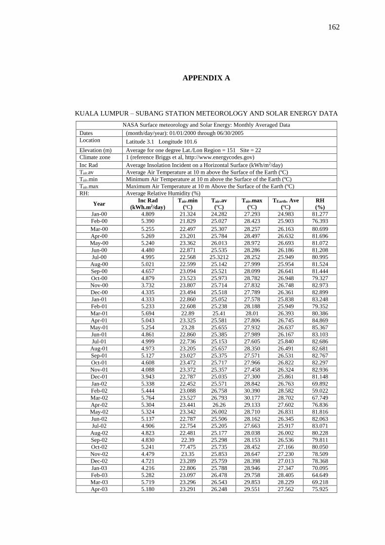
162
APPENDIX A
KUALA LUMPUR – SUBANG STATION METEOROLOGY AND SOLAR ENERGY DATA
NASA Surface meteorology and Solar Energy: Monthly Averaged Data
Dates (month/day/year): 01/01/2000 through 06/30/2005
Location Latitude 3.1 Longitude 101.6
Elevation (m) Average for one degree Lat./Lon Region = 151 Site = 22
Climate zone 1 (reference Briggs et al, http://www.energycodes.gov)
Inc Rad Average Insolation Incident on a Horizontal Surface (kWh/m2/day)
Tair.av Average Air Temperature at 10 m above the Surface of the Earth (ºC)
Tair.min Minimum Air Temperature at 10 m above the Surface of the Earth (ºC)
Tair.max Maximum Air Temperature at 10 m Above the Surface of the Earth (ºC)
RH: Average Relative Humidity (%)
Year Inc Rad
(kWh.m2/day)
Tair.min
(ºC)
Tair.av
(ºC)
Tair.max
(ºC)
TEarth. Ave
(ºC)
RH
(%)
Jan-00 4.809 21.324 24.282 27.293 24.983 81.277
Feb-00 5.390 21.829 25.027 28.423 25.903 76.393
Mar-00 5.255 22.497 25.307 28.257 26.163 80.699
Apr-00 5.269 23.201 25.784 28.497 26.632 81.696
May-00 5.240 23.362 26.013 28.972 26.693 81.072
Jun-00 4.480 22.871 25.535 28.286 26.186 81.208
Jul-00 4.995 22.568 25.3212 28.252 25.949 80.995
Aug-00 5.021 22.599 25.142 27.999 25.954 81.524
Sep-00 4.657 23.094 25.521 28.099 26.641 81.444
Oct-00 4.879 23.523 25.973 28.782 26.948 79.327
Nov-00 3.732 23.807 25.714 27.832 26.748 82.973
Dec-00 4.335 23.494 25.518 27.789 26.361 82.899
Jan-01 4.333 22.860 25.052 27.578 25.838 83.248
Feb-01 5.233 22.608 25.238 28.188 25.949 79.352
Mar-01 5.694 22.89 25.41 28.01 26.393 80.386
Apr-01 5.043 23.325 25.581 27.806 26.745 84.869
May-01 5.254 23.28 25.655 27.932 26.637 85.367
Jun-01 4.861 22.860 25.385 27.989 26.167 83.103
Jul-01 4.999 22.736 25.153 27.605 25.840 82.686
Aug-01 4.973 23.205 25.657 28.350 26.491 82.681
Sep-01 5.127 23.027 25.375 27.571 26.531 82.767
Oct-01 4.608 23.472 25.717 27.966 26.822 82.297
Nov-01 4.088 23.372 25.357 27.458 26.324 82.936
Dec-01 3.943 22.787 25.035 27.300 25.861 81.148
Jan-02 5.338 22.452 25.571 28.842 26.763 69.892
Feb-02 5.444 23.088 26.758 30.390 28.582 59.022
Mar-02 5.764 23.527 26.793 30.177 28.702 67.749
Apr-02 5.304 23.441 26.26 29.133 27.602 76.836
May-02 5.324 23.342 26.002 28.710 26.831 81.816
Jun-02 5.137 22.787 25.506 28.162 26.345 82.063
Jul-02 4.906 22.754 25.205 27.663 25.917 83.071
Aug-02 4.823 22.481 25.177 28.038 26.002 80.228
Sep-02 4.830 22.39 25.298 28.153 26.536 79.811
Oct-02 5.241 77.475 25.735 28.452 27.166 80.050
Nov-02 4.479 23.35 25.853 28.647 27.230 78.509
Dec-02 4.721 23.289 25.759 28.398 27.013 78.368
Jan-03 4.216 22.806 25.788 28.946 27.347 70.095
Feb-03 5.282 23.097 26.478 29.758 28.405 64.649
Mar-03 5.719 23.296 26.543 29.853 28.229 69.218
Apr-03 5.180 23.291 26.248 29.551 27.562 75.925

163
May-03 5.087 23.601 26.6671 30.12 27.625 75.424
Jun-03 4.835 22.479 25.455 28.426 26.573 77.678
Jul-03 4.592 22.737 25.754 29.123 26.920 75.337
Aug-03 4.873 22.787 25.370 28.153 26.383 80.104
Sep-03 4.486 22.647 25.297 27.945 26.622 79.712
Oct-03 4.510 23.172 25.819 28.745 27.131 76.669
Nov-03 4.334 23.509 25.987 28.821 27.509 76.624
Dec-03 3.827 23.432 26.309 29.478 28.174 66.728
Jan-04 5.345 23.981 27.436 30.979 30.127 57.632
Feb-04 5.338 23.872 27.564 31.662 30.006 57.156
Mar-04 5.462 24.211 27.519 31.091 29.775 72.132
Apr-04 5.293 24.567 28.131 31.979 30.404 62.458
May-04 5.346 24.403 28.197 31.698 30.211 59.925
Jun-04 4.7563 22.552 26.309 30.069 27.636 68.495
Jul-04 4.599 22.613 26.019 29.45 27.786 69.562
Aug-04 5.322 22.419 25.556 28.821 27.093 74.610
Sep-04 5.082 22.851 25.959 29.027 27.941 71.673
Oct-04 5.025 23.403 26.539 29.793 28.917 68.167
Nov-04 4.539 24.423 27.414 30.476 30.382 62.612
Dec-04 3.775 24.324 27.397 30.591 30.353 58.124
Jan-05 5.435 23.69 27.421 30.807 30.296 53.760
Feb-05 5.823 24.016 27.363 30.433 29.977 58.869
Mar-05 5.759 23.886 27.163 30.420 29.287 65.451
Apr-05 5.600 23.096 25.951 28.957 27.164 79.654
May-05 4.977 23.128 25.891 28.800 26.904 80.82
Jun-05 4.935 22.951 25.812 28.863 26.454 78.897
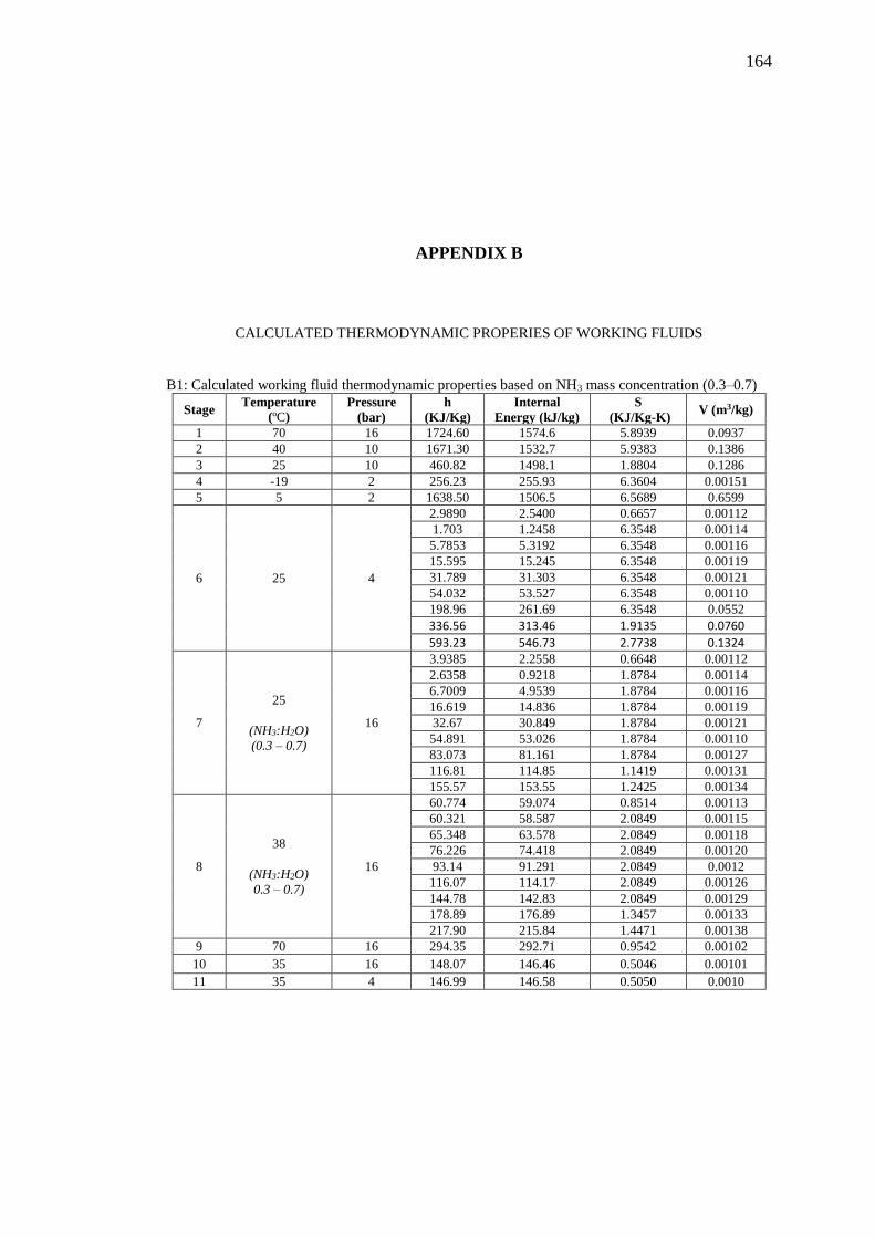
164
APPENDIX B
CALCULATED THERMODYNAMIC PROPERIES OF WORKING FLUIDS
B1: Calculated working fluid thermodynamic properties based on NH3 mass concentration (0.3–0.7)
Stage Temperature
(ºC)
Pressure
(bar)
h
(KJ/Kg)
Internal
Energy (kJ/kg)
S
(KJ/Kg-K) V (m3/kg)
1 70 16 1724.60 1574.6 5.8939 0.0937
2 40 10 1671.30 1532.7 5.9383 0.1386
3 25 10 460.82 1498.1 1.8804 0.1286
4 -19 2 256.23 255.93 6.3604 0.00151
5 5 2 1638.50 1506.5 6.5689 0.6599
6 25 4
2.9890 2.5400 0.6657 0.00112
1.703 1.2458 6.3548 0.00114
5.7853 5.3192 6.3548 0.00116
15.595 15.245 6.3548 0.00119
31.789 31.303 6.3548 0.00121
54.032 53.527 6.3548 0.00110
198.96 261.69 6.3548 0.0552
336.56 313.46 1.9135 0.0760
593.23 546.73 2.7738 0.1324
7
25
(NH3:H2O)
(0.3 – 0.7)
16
3.9385 2.2558 0.6648 0.00112
2.6358 0.9218 1.8784 0.00114
6.7009 4.9539 1.8784 0.00116
16.619 14.836 1.8784 0.00119
32.67 30.849 1.8784 0.00121
54.891 53.026 1.8784 0.00110
83.073 81.161 1.8784 0.00127
116.81 114.85 1.1419 0.00131
155.57 153.55 1.2425 0.00134
8
38
(NH3:H2O)
0.3 – 0.7)
16
60.774 59.074 0.8514 0.00113
60.321 58.587 2.0849 0.00115
65.348 63.578 2.0849 0.00118
76.226 74.418 2.0849 0.00120
93.14 91.291 2.0849 0.0012
116.07 114.17 2.0849 0.00126
144.78 142.83 2.0849 0.00129
178.89 176.89 1.3457 0.00133
217.90 215.84 1.4471 0.00138
9 70 16 294.35 292.71 0.9542 0.00102
10 35 16 148.07 146.46 0.5046 0.00101
11 35 4 146.99 146.58 0.5050 0.0010

165
B2: Calculated working fluid thermodynamic properties at turbine inlet pressure (12 – 15bar)
Stage Temperature
(ºC)
Pressure
(bar)
h
(KJ/Kg)
Internal Energy
(kJ/kg)
S
(KJ/Kg-K) V (m3/kg)
1 70 12 – 21
1742.8 1588.1 6.0748 0.129
1738.3 1584.8 6.0259 0.118
1733.8 1581.5 5.9797 0.109
1729.2 1578.1 5.9358 0.101
1724.6 1574.6 5.8939 0.094
1719.8 1571.1 5.8537 0.0875
1715.00 1567.50 5.8149 0.0819
1710.1 1563.9 5.7775 0.0769
1705.1 1560.1 5.7411 0.0725
1699.9 1556.3 5.7057 0.0684
2 40 10 1671.3 1532.7 5.9383 0.139
3 25 10 460.82 1498.1 1.8804 0.0016
4 -19 2 256.23 255.93 6.3604 0.0015
5 5 2 1638.5 1506.5 6.5689 0.659
6 25 4 54.032 53.527 6.3548 0.0011
7 25 12 – 21
12.000 16.374 14.947 0.822
16.455 14.910 0.8219 0.00119
16.537 14.873 0.8218 0.00119
16.619 14.836 0.8217 0.00119
16.700 14.799 0.8215 0.00119
16.782 14.762 0.8214 0.00119
16.864 14.725 0.8213 0.00119
16.945 14.688 0.8212 0.00119
17.027 14.651 0.8211 0.00119
17.109 14.614 0.8209 0.00119
8 38 12 – 21
75.989 74.542 1.0178 0.00121
76.068 74.501 1.0176 0.00121
76.147 74.459 1.0175 0.00121
76.226 74.418 1.0174 0.00121
76.305 74.376 1.0172 0.00121
76.384 74.335 1.0171 0.00121
76.463 74.294 1.0170 0.00121
76.542 74.252 1.0168 0.00121
76.621 74.211 1.0167 0.00121
76.700 74.170 1.0166 0.00120
9 70 12 – 21
294.02 292.79 0.9544 0.00102
294.10 292.77 0.9544 0.00102
294.18 292.75 0.9543 0.00102
294.27 292.73 0.9543 0.00102
294.35 292.71 0.9542 0.00102
294.43 292.69 0.9541 0.00102
294.51 292.67 0.9541 0.00102
294.59 292.65 0.9540 0.00102
294.68 292.63 0.9539 0.00102
294.76 292.61 0.9539 0.00102
10 35 12 – 21
147.71 146.50 0.5047 0.00101
147.80 146.49 0.5046 0.00101
147.89 146.48 0.5046 0.00101
147.98 146.47 0.5046 0.00101
148.07 146.46 0.5046 0.00101
148.16 146.45 0.5045 0.001001
148.25 146.44 0.5045 0.001001
148.34 146.43 0.5045 0.001001
148.43 146.42 0.5044 0.001001
148.52 146.40 0.5044 0.001001
11 35 4 146.99 146.58 0.5049 0.001006
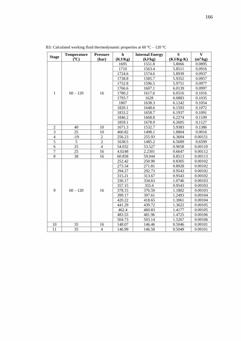
166
B3: Calculated working fluid thermodynamic properties at 60 ºC – 120 ºC
Stage Temperature
(0C)
Pressure
(bar)
h
(KJ/Kg)
Internal Energy
(kJ/kg)
S
(KJ/Kg-K)
V
(m3/kg)
1 60 – 120 16
1695 1551.8 5.8066 0.0895
1710 1563.4 5.8511 0.0916
1724.6 1574.6 5.8939 0.0937
1738.8 1585.7 5.9352 0.0957
1752.8 1596.5 5.9751 0.0977
1766.6 1607.1 6.0139 0.0997
1780.2 1617.6 6.0516 0.1016
1793.7 1628 6.0883 0.1035
1807 1638.3 6.1242 0.1054
1820.1 1648.6 6.1593 0.1072
1833.2 1658.7 6.1937 0.1091
1846.2 1668.8 6.2274 0.1109
1859.1 1678.9 6.2605 0.1127
2 40 10 1671.3 1532.7 5.9383 0.1386
3 25 10 460.82 1498.1 1.8804 0.0016
4 -19 2 256.23 255.93 6.3604 0.00151
5 5 2 1638.5 1485.2 6.5689 0.6599
6 25 4 54.032 53.527 0.9658 0.00110
7 25 16 4.0248 2.2301 0.6647 0.00112
8 38 16 60.858 59.044 0.8513 0.00113
9 60 – 120 16
252.42 250.90 0.8305 0.00102
273.34 271.81 0.8928 0.00102
294.27 292.73 0.9543 0.00102
315.21 313.67 0.9543 0.00102
336.17 334.63 1.0746 0.00103
357.15 355.6 0.9543 0.00103
378.15 376.59 1.1802 0.00103
399.17 397.61 1.2493 0.00104
420.22 418.65 1.3061 0.00104
441.29 439.72 1.3622 0.00105
462.4 460.83 1.4177 0.00105
483.55 481.96 1.4725 0.00106
504.73 503.14 1.5267 0.00106
10 35 16 148.07 146.46 0.5046 0.00101
11 35 4 146.99 146.58 0.5049 0.00101

167
APPENDIX C
C# SOLUTION ALGORITHM AND CALCULATION IMPLEMENTATION
C1: Flowchat fot the proposed System Capacity Model Calculation in C#
C2: Calculation Algorithm in C#
#region Pcc model instance
public PlantCoolingCapacityModel Pcc { get; private set; }
#endregion
#region Compute Parameters
public ICommand ComputeParameters { get; private set; }
public bool CanComputeParameters =>
!Pcc.IsComputed && _Q_inc_Ave != 0 && Pcc.Q_evp != 0 && Pcc.T_r != 0
&& _load_h_instance.LoadedValues != null && Pcc.X_NH3 != 0 && Pcc.n_g != 0 && Pcc.n_t
!= 0
&& Pcc.n_sp != 0 && Pcc.P_6 != 0 && Pcc.P_7 != 0 && Pcc.V_7 != 0 && Pcc.k_c != 0;
public void ComputeParametersVal() {
lock (Pcc) {
Thread thread = new Thread(() => {
Soil Cooling Load Plant Cooling Capacity Pipe (Earth Tube) Cooling Capacity
Start
Input Air Temp, Solar Rad for selected time
Input fixed parameters (Ur, d, Z, Zom, hc, R, Mw, K, ql, w, , )
Calc. Latent heat flux [QL(t)]
Calc. Sensible heat flux [Qh(t)]
Calc. Net Rad Flux [Rn(t)]
Cooling load
[Qload(t)]
Calc. enthalpy (h), entropy (S) & Vol.(V) @ selected temps & Pressures
Calc. collector energy potential (Qu) and Area (As) for the plant capacity
Get Quotations based on all components sizes
Quotation ≤ Budget?
Proceed with selected plant capacity
Plant size = selected Qevp
Select Pipe nominal size (Radius & Thickness)
Input Pipe and Soil thermal parameters (Nu, Ks, Kp, Kw, ds)
Select Chilled water & Pipe external wall Temps (Tw& Tp)
Calc. Chilled water-Pipe heat
transfer resistance (R1)
Calc. Pipe inner-outer walls heat transfer
resistance (R2) Calc. Pipe-Soil
heat transfer resistance (R3)
Calc. Pipe heat transfer coefficient [UA=1/(R1+R2+R3)]
Calc. Pipe Cooling Capacity (Qsw)
Pipe Cooling (Qsw)
Divide Cooling capacity (Qevp) by Pipe cooling capacity (Qsw)
Pipe Length (l)
End
Set plant operating Temps Pressures
Select working fluid (W/F) & conc.
ratio
Estimate Plant Capacity (Qevp) Get Location Weather Data
Select Calculation period (hr.)
Cal soil heat flux [Qs(t)]
Multiply [Qs(t)] by Safety factor ( )
Calc. Plant components energy balance @ (Qt, Wt, Qabs, Qb, Qhx) to determine the capacity
Calc. mr, mwt, & msolfor the W/F
Input Ave Solar Rad [(Qinc(ave.)]
Reduce As
Calculate Cooling load Average [Qload(ave)]
Select soil bed size (As)
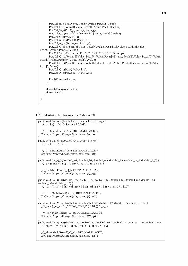
168
Pcc.Cal_m_r(Pcc.Q_evp, Pcc.h[4].Value, Pcc.h[2].Value);
Pcc.Cal_Q_t(Pcc.m[0].Value, Pcc.h[0].Value, Pcc.h[1].Value);
Pcc.Cal_W_t(Pcc.Q_t, Pcc.n_t, Pcc.n_g);
Pcc.Cal_Q_c(Pcc.m[1].Value, Pcc.h[1].Value, Pcc.h[2].Value);
Pcc.Cal_CR(Pcc.X_NH3);
Pcc.Cal_m_sol(Pcc.CR, Pcc.m_r);
Pcc.Cal_m_wt(Pcc.m_sol, Pcc.m_r);
Pcc.Cal_Q_abs(Pcc.m[4].Value, Pcc.h[4].Value, Pcc.m[10].Value, Pcc.h[10].Value,
Pcc.m[5].Value, Pcc.h[5].Value);
Pcc.Cal_W_sp(Pcc.m_sol, Pcc.V_7, Pcc.P_7, Pcc.P_6, Pcc.n_sp);
Pcc.Cal_Q_hx(Pcc.m[6].Value, Pcc.h[6].Value, Pcc.m[8].Value, Pcc.h[8].Value, Pcc.m[7].Value,
Pcc.h[7].Value, Pcc.m[9].Value, Pcc.h[9].Value);
Pcc.Cal_Q_b(Pcc.m[0].Value, Pcc.h[0].Value, Pcc.m[8].Value, Pcc.h[8].Value, Pcc.m[7].Value,
Pcc.h[7].Value);
Pcc.Cal_Q_u(Pcc.Q_b, Pcc.k_c);
Pcc.Cal_A_c(Pcc.Q_u, _Q_inc_Ave);
Pcc.IsComputed = true;
});
thread.IsBackground = true;
thread.Start();
}
}
C3: Calculation Implementation Codes in C#
public void Cal_A_c(double l_Q_u, double l_Q_inc_avg) {
_A_c = l_Q_u / (l_Q_inc_avg * 0.001);
_A_c = Math.Round(_A_c, DECIMALPLACES);
OnOutputPropertyChanged(this, nameof(A_c));
}
public void Cal_Q_u(double l_Q_b, double l_k_c) {
_Q_u = l_Q_b / l_k_c;
_Q_u = Math.Round(_Q_u, DECIMALPLACES);
OnOutputPropertyChanged(this, nameof(Q_u));
}
public void Cal_Q_b(double l_m1, double l_h1, double l_m9, double l_h9, double l_m_8, double l_h_8) {
_Q_b = (l_m1 * l_h1) + (l_m9 * l_h9) - (l_m_8 * l_h_8);
_Q_b = Math.Round(_Q_b, DECIMALPLACES);
OnOutputPropertyChanged(this, nameof(Q_b));
}
public void Cal_Q_hx(double l_m7, double l_h7, double l_m9, double l_h9, double l_m8, double l_h8,
double l_m10, double l_h10) {
_Q_hx = ((l_m7 * l_h7) + (l_m9 * l_h9)) - ((l_m8 * l_h8) + (l_m10 * l_h10));
_Q_hx = Math.Round(_Q_hx, DECIMALPLACES);
OnOutputPropertyChanged(this, nameof(Q_hx));
}
public void Cal_W_sp(double l_m_sol, double l_V7, double l_P7, double l_P6, double l_n_sp) {
_W_sp = (l_m_sol * l_V7 * ((l_P7 - l_P6) * 100)) / l_n_sp;
_W_sp = Math.Round(_W_sp, DECIMALPLACES);
OnOutputPropertyChanged(this, nameof(W_sp));
}
public void Cal_Q_abs(double l_m5, double l_h5, double l_m11, double l_h11, double l_m6, double l_h6) {
_Q_abs = (l_m5 * l_h5) + (l_m11 * l_h11) - (l_m6 * l_h6);
_Q_abs = Math.Round(_Q_abs, DECIMALPLACES);
OnOutputPropertyChanged(this, nameof(Q_abs));
}

169
public void Cal_m_wt(double l_m_sol, double l_m_r) {
_m_wt = (l_m_sol - l_m_r);
_m_wt = Math.Round(_m_wt, DECIMALPLACES);
_m[8].Value = _m[9].Value = _m[10].Value = _m_wt;
OnOutputPropertyChanged(this, nameof(m_wt));
}
public void Cal_m_sol(double l_CR, double l_m_r) {
_m_sol = (l_CR * l_m_r);
_m_sol = Math.Round(_m_sol, DECIMALPLACES);
_m[5].Value = _m[6].Value = _m[7].Value = _m_sol;
OnOutputPropertyChanged(this, nameof(m_sol));
}
public void Cal_CR(double l_X_NH3) {
_CR = 1 / l_X_NH3;
_CR = Math.Round(_CR, DECIMALPLACES);
OnOutputPropertyChanged(this, nameof(CR));
}
public void Cal_Q_c(double l_m2, double l_h2, double l_h3) {
_Q_c = l_m2 * (l_h2 - l_h3);
_Q_c = Math.Round(_Q_c, DECIMALPLACES);
OnOutputPropertyChanged(this, nameof(Q_c));
}
public void Cal_W_t(double l_Q_t, double l_n_t, double l_n_g) {
_W_t = l_Q_t * l_n_t * l_n_g;
_W_t = Math.Round(_W_t, DECIMALPLACES);
OnOutputPropertyChanged(this, nameof(W_t));
}
public void Cal_Q_t(double l_m1, double l_h1, double l_h2) {
_Q_t = l_m1 * (l_h1 - l_h2);
_Q_t = Math.Round(_Q_t, DECIMALPLACES);
OnOutputPropertyChanged(this, nameof(Q_t));
}
public void Cal_m_r(double l_Q_evp, double l_h5, double l_h3) {
_m_r = (l_Q_evp / (l_h5 - l_h3));
_m_r = Math.Round(_m_r, DECIMALPLACES);
_m[0].Value = _m[1].Value = _m[2].Value = _m[3].Value = _m[4].Value = _m_r;
OnOutputPropertyChanged(this, nameof(m_r));
}
public bool Compare_Budget_Quotation(double l_budget, double l_quotation) {
return (l_quotation <= l_budget);
}

170
APPENDIX D
EXPERIMENTAL SET-UPS
Chilled Water Tanks, Cooled Soil bed, and Controlled Soil Bed
Soil Data logging to Computer through NI Data Logger
Absorption Chiller Operating Data Logging to Computer through NI Logger

171
APPENDIX E
SOIL COOLING TEMPERATURE PROFILE
0
5
10
15
20
25
30
35
40
45
50
6:00
6:2
26
:4
47:06
7:2
87:50
8:1
28:34
8:5
69:18
9:4
01
0:0
210:24
10
:4
611:08
11
:3
011:52
12
:1
412:36
12
:5
81
3:2
013:42
14
:0
414:26
14
:4
815:10
15
:3
215:54
16
:1
61
6:3
817:00
17
:2
217:44
18
:0
618:28
18
:5
01
9:1
219:34
19
:5
620:18
20
:4
0
Tem
pera
tu
re (
℃)
Time (min)
Chilled Water Inlet Chilled Water Return Ambient Air Soil Bed Point 1 Soil Bed Point 2
Soil Bed Point 3 Soil Bed Point 4 Uncooled Soil Soil Bed at 50mm Cntrol Bed at 50mm
Flow rate = 0.004kg/sec
0
5
10
15
20
25
30
35
40
45
50
6:0
06
:22
6:4
47
:06
7:2
87
:50
8:1
28
:34
8:5
69
:18
9:4
01
0:0
21
0:2
41
0:4
61
1:0
81
1:3
01
1:5
21
2:1
41
2:3
61
2:5
81
3:2
01
3:4
21
4:0
41
4:2
61
4:4
81
5:1
01
5:3
21
5:5
41
6:1
61
6:3
81
7:0
01
7:2
21
7:4
41
8:0
61
8:2
81
8:5
01
9:1
21
9:3
41
9:5
62
0:1
82
0:4
02
1:0
2
Tem
pera
tu
re (
℃)
Time (min)
Chilled Water Inlet Chilled Water Return Ambient Air Soil Bed Point 1 Soil Bed Point 2
Soil Bed Point 3 Soil Bed Point 4 Uncooled Soil Soil Bed at 50mm Cntrol Bed at 50mm
Flow rate = 0.006kg/sec
0
5
10
15
20
25
30
35
40
45
6:1
3
6:3
6
6:5
9
7:2
2
7:4
5
8:0
8
8:3
1
8:5
4
9:1
7
9:4
0
10
:03
10
:26
10
:49
11
:12
11
:35
11
:58
12
:21
12
:44
13
:07
13
:30
13
:53
14
:16
14
:39
15
:02
15
:25
15
:48
16
:11
16
:34
16
:57
17
:20
17
:43
18
:06
18
:29
18
:52
19
:15
19
:38
20
:01
Te
mp
era
to
re
℃)
Time (min)
Chilled Water Inlet Chilled Water Return Ambient Air Soil Bed Point 1 Soil Bed Point 2
Soil Bed Point 3 Soil Bed Point 4 Controled Soil Cntrol Bed at 50mm Soil Bed at 50mm
Flow rate = 0.008kg/sec
0
5
10
15
20
25
30
35
40
45
50
6:0
0
6:2
6
6:5
2
7:1
8
7:4
4
8:1
0
8:3
6
9:0
2
9:2
8
9:5
4
10
:2
0
10
:4
6
11
:1
2
11
:3
8
12
:0
4
12
:3
0
12
:5
6
13
:2
2
13
:4
8
14
:1
4
14
:4
0
15
:0
6
15
:3
2
15
:5
8
16
:2
4
16
:5
0
17
:1
6
17
:4
2
18
:0
8
18
:3
4
19
:0
0
19
:2
6
19
:5
2
20
:1
8
20
:4
4
21
:1
0
21
:3
6
22
:0
2
Te
mp
era
tu
re
(℃
)
Time (min)
Chilled Water Inlet Chilled Water Return Ambient Air Soil Bed Point 1 Soil Bed Point 2
Soil Bed Point 3 Soil Bed Point 4 Uncooled Soil Soil Bed at 50mm Cntrol Bed at 50mm
Flow rate = 0.01kg/sec

172
APPENDIX F
AB ORPTIONنCHILLER’ نPERFORMANCE
-40
-20
0
20
40
60
80
100
120
140
160
1 6 11 16 21 26 31 36 41 46 51 56 61
Tem
pera
tu
re (
℃)
Time (min)
Evaporator Temp Amb Air Temp Heat Source Temp Cond Inlet Temp
Cond Exit Temp Absorber Temp HX Temp
Chiller’sنPerformanceن (1st Run)
-40
-20
0
20
40
60
80
100
120
140
160
1 6 11 16 21 26 31 36 41 46 51 56 61
Tem
pera
tu
re (
℃)
Time (min)
Evaporator Temp Amb Air Temp Heat Source Temp Cond Inlet Temp
Cond Exit Temp Absorber Temp HX Temp
Chiller’sنPerformanceن (2nd Run)
-40
-20
0
20
40
60
80
100
120
140
160
1 6 11 16 21 26 31 36 41 46 51 56 61
Tem
pera
tu
re (
℃)
Time (min)
Evaporator Temp Amb Air Temp Heat Source Temp Cond Inlet Temp
Cond Exit Temp Absorber Temp HX Temp
Chiller’sPerformance (3rd Run)
-40
-20
0
20
40
60
80
100
120
140
160
1 6 11 16 21 26 31 36 41 46 51 56 61
Tem
peratu
re (
℃)
Time (min)
Evaporator Temp Amb Air Temp Heat Source Temp Cond Inlet Temp
Cond Exit Temp Absorber Temp HX Temp
Chiller’sنPerformanceن(4thنRun)
-40
-20
0
20
40
60
80
100
120
140
160
1 3 5 7 9 11 13 15 17 19 21 23 25 27 29 31 33 35 37 39 41 43 45 47 49 51 53 55 57 59 61 63
Tem
peratu
re (
℃)
Time (min)
Evaporator Temp Amb Air Temp Heat Source Temp Cond Inlet Temp
Cond Exit Temp Absorber Temp HX Temp
Chiller’sنPerformance5)نth Run)
-40
-20
0
20
40
60
80
100
120
140
160
1 6 11 16 21 26 31 36 41 46 51 56 61
Tem
pera
ture (
℃)
Time (min)
Evaporator Temp Amb Air Temp Heat Source Temp Cond Inlet Temp
Cond Exit Temp Absorber Temp HX Temp
Chiller’sنPerformance6)نth Run)
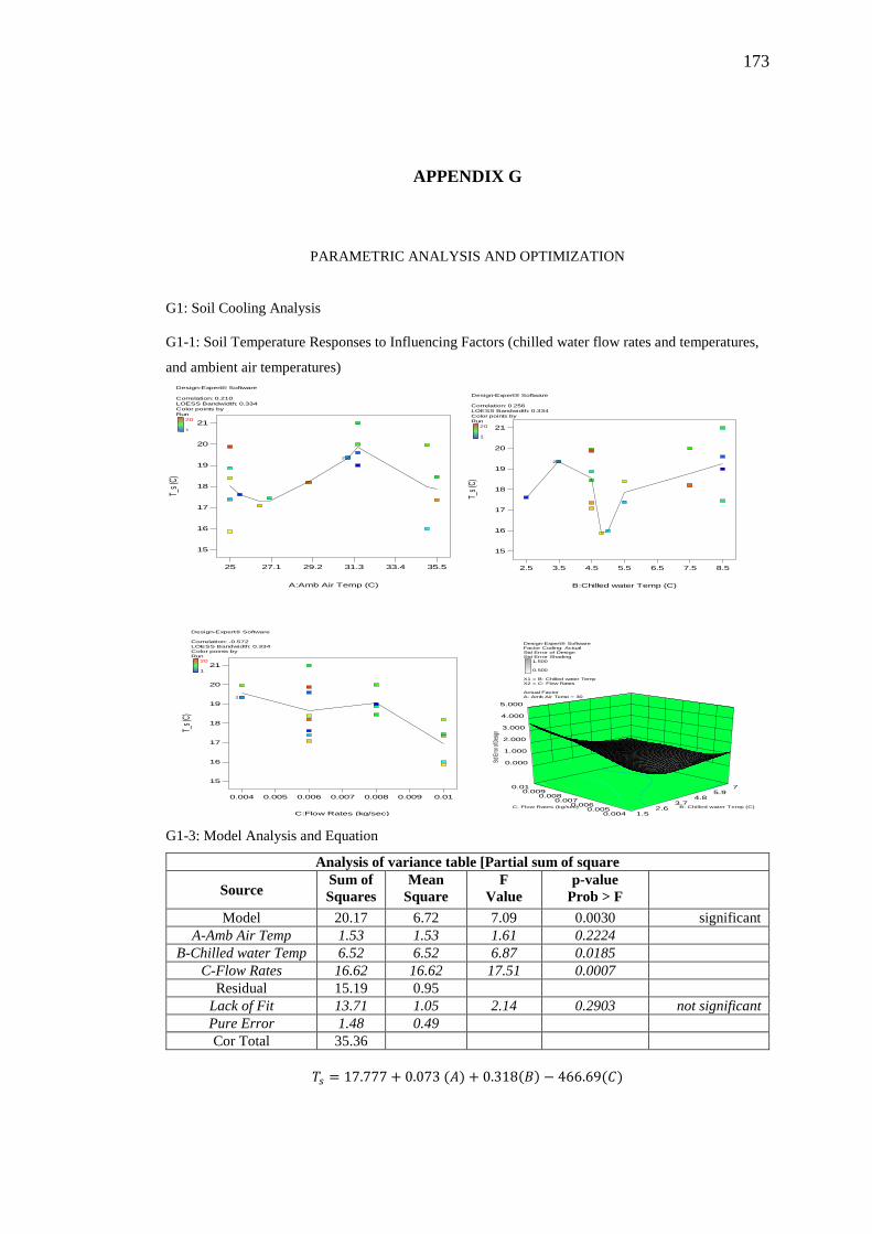
173
APPENDIX G
PARAMETRIC ANALYSIS AND OPTIMIZATION
G1: Soil Cooling Analysis
G1-1: Soil Temperature Responses to Influencing Factors (chilled water flow rates and temperatures,
and ambient air temperatures)
G1-3: Model Analysis and Equation
Analysis of variance table [Partial sum of square
Source Sum of
Squares
Mean
Square
F
Value
p-value
Prob > F
Model 20.17 6.72 7.09 0.0030 significant
A-Amb Air Temp 1.53 1.53 1.61 0.2224
B-Chilled water Temp 6.52 6.52 6.87 0.0185
C-Flow Rates 16.62 16.62 17.51 0.0007
Residual 15.19 0.95
Lack of Fit 13.71 1.05 2.14 0.2903 not significant
Pure Error 1.48 0.49
Cor Total 35.36
𝑇𝑠 = 17.777 + 0.073 (𝐴) + 0.318(𝐵) − 466.69(𝐶)
Design-Expert® Software
Correlation: 0.210
LOESS Bandwidth: 0.334
Color points by
Run
20
1
2
25 27.1 29.2 31.3 33.4 35.5
15
16
17
18
19
20
21
A:Amb Air Temp (C)
T_s
(C)
Design-Expert® Software
Correlation: 0.210
LOESS Bandwidth: 0.334
Color points by
Run
20
1
2
25 27.1 29.2 31.3 33.4 35.5
15
16
17
18
19
20
21
A:Amb Air Temp (C)
T_s
(C)
Design-Expert® Software
Correlation: 0.256
LOESS Bandwidth: 0.334
Color points by
Run
20
1
2
2.5 3.5 4.5 5.5 6.5 7.5 8.5
15
16
17
18
19
20
21
B:Chilled water Temp (C)
T_s
(C)
Design-Expert® Software
Correlation: 0.256
LOESS Bandwidth: 0.334
Color points by
Run
20
1
2
2.5 3.5 4.5 5.5 6.5 7.5 8.5
15
16
17
18
19
20
21
B:Chilled water Temp (C)
T_s
(C)
Design-Expert® Software
Correlation: -0.572
LOESS Bandwidth: 0.334
Color points by
Run
20
1
2
0.004 0.005 0.006 0.007 0.008 0.009 0.01
15
16
17
18
19
20
21
C:Flow Rates (kg/sec)
T_s (
C)
Design-Expert® Software
Correlation: -0.572
LOESS Bandwidth: 0.334
Color points by
Run
20
1
2
0.004 0.005 0.006 0.007 0.008 0.009 0.01
15
16
17
18
19
20
21
C:Flow Rates (kg/sec)
T_s (
C)
Design-Expert® Software
Factor Coding: Actual
Std Error of Design
Std Error Shading
1.500
0.500
X1 = B: Chilled water Temp
X2 = C: Flow Rates
Actual Factor
A: Amb Air Temp = 30
0.004 0.005
0.006 0.007
0.008 0.009
0.01
1.5 2.6
3.7 4.8
5.9 7
0.000
1.000
2.000
3.000
4.000
5.000
Std
Erro
r of D
esig
n
B: Chilled water Temp (C)C: Flow Rates (kg/sec)
Design-Expert® Software
Factor Coding: Actual
Std Error of Design
Std Error Shading
1.500
0.500
X1 = B: Chilled water Temp
X2 = C: Flow Rates
Actual Factor
A: Amb Air Temp = 30
0.004 0.005
0.006 0.007
0.008 0.009
0.01
1.5 2.6
3.7 4.8
5.9 7
0.000
1.000
2.000
3.000
4.000
5.000
Std
Erro
r of D
esign
B: Chilled water Temp (C)C: Flow Rates (kg/sec)

174
G1-4: Model Diagnostics and Graph
G2: Combined Plant Analysis
G2-1: Plant Performance Responses (W_t, W_sp, Q_loss, COP_cooling, ORC_eff, and COP_overall) to
influencing factors (W/F temperatures, Boiler pressure, and W/F concentration ratio)
Design-Expert® Software
T_s
Lambda
Current = 1
Best = 1.61
Low C.I. = -3.95
High C.I. = 7.16
Recommend transform:
None
(Lambda = 1)
Lambda
Ln(R
esid
ualS
S)
Box-Cox Plot for Power Transforms
2.7
2.75
2.8
2.85
2.9
2.95
3
-3 -2 -1 0 1 2 3
2.95754
Design-Expert® Software
T_s
Lambda
Current = 1
Best = 1.61
Low C.I. = -3.95
High C.I. = 7.16
Recommend transform:
None
(Lambda = 1)
Lambda
Ln(R
esid
ualS
S)
Box-Cox Plot for Power Transforms
2.7
2.75
2.8
2.85
2.9
2.95
3
-3 -2 -1 0 1 2 3
2.95754
Design-Expert® Software
Factor Coding: Actual
T_s (C)
20.996
15.864
X1 = A: Amb Air Temp
X2 = B: Chilled water Temp
Actual Factor
C: Flow Rates = 0.007
1.5 2.6
3.7 4.8
5.9 7
25 27
29 31
33 35
15
16
17
18
19
20
21
T_s (
C)
A: Amb Air Temp (C)B: Chilled water Temp (C)
Design-Expert® Software
Factor Coding: Actual
T_s (C)
20.996
15.864
X1 = A: Amb Air Temp
X2 = B: Chilled water Temp
Actual Factor
C: Flow Rates = 0.007
1.5 2.6
3.7 4.8
5.9 7
25 27
29 31
33 35
15
16
17
18
19
20
21
T_s (
C)
A: Amb Air Temp (C)B: Chilled water Temp (C)
Design-Expert® Software
Correlation: 0.072
LOESS Bandwidth: 0.334
Color points by
Run
23
12
2
2
22
65 72 79 86 93 100
5E-005
0.0001
0.00015
0.0002
0.00025
0.0003
0.00035
A:W/F Temp (C)
W_s
p (W
)
Design-Expert® Software
Correlation: 0.072
LOESS Bandwidth: 0.334
Color points by
Run
23
12
2
2
22
65 72 79 86 93 100
5E-005
0.0001
0.00015
0.0002
0.00025
0.0003
0.00035
A:W/F Temp (C)
W_s
p (W
)
Design-Expert® Software
Correlation: 1.000
LOESS Bandwidth: 0.334
Color points by
Run
23
1
3
5
5
2
3
65 72 79 86 93 100
0.002
0.003
0.004
0.005
0.006
A:W/F Temp (C)
W_t
(W)
Design-Expert® Software
Correlation: 1.000
LOESS Bandwidth: 0.334
Color points by
Run
23
1
3
5
5
2
3
65 72 79 86 93 100
0.002
0.003
0.004
0.005
0.006
A:W/F Temp (C)
W_t
(W)
Design-Expert® Software
Correlation: 0.579
LOESS Bandwidth: 0.334
Color points by
Run
23
12
2
2
2
2
2
65 72 79 86 93 100
-0.005
0
0.005
0.01
0.015
0.02
0.025
A:W/F Temp (C)
Q_l
oss
(W)
Design-Expert® Software
Correlation: 0.579
LOESS Bandwidth: 0.334
Color points by
Run
23
12
2
2
2
2
2
65 72 79 86 93 100
-0.005
0
0.005
0.01
0.015
0.02
0.025
A:W/F Temp (C)
Q_l
oss
(W)
Design-Expert® Software
Correlation: -0.429
LOESS Bandwidth: 0.334
Color points by
Run
23
1
2
2
2 2
2
2
65 72 79 86 93 100
0.45
0.5
0.55
0.6
0.65
0.7
A:W/F Temp (C)
COP_
cool
ing
Design-Expert® Software
Correlation: -0.429
LOESS Bandwidth: 0.334
Color points by
Run
23
1
2
2
2 2
2
2
65 72 79 86 93 100
0.45
0.5
0.55
0.6
0.65
0.7
A:W/F Temp (C)
COP_
cool
ing
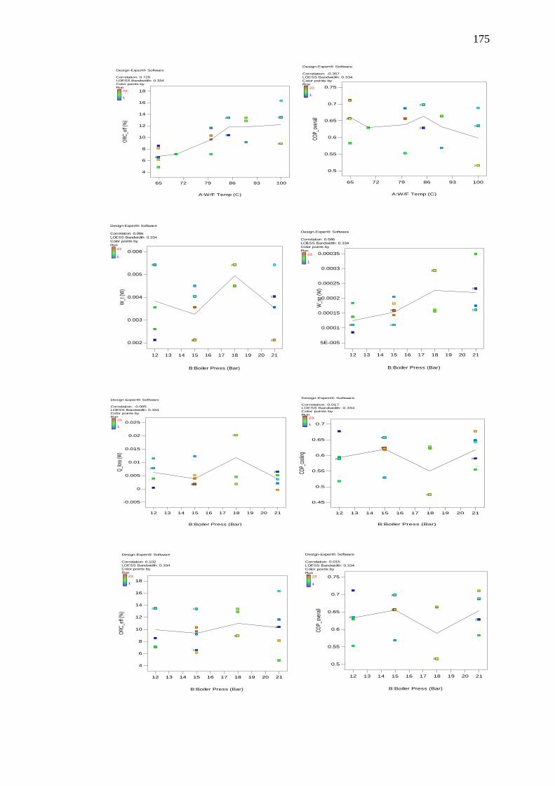
175
Design-Expert® Software
Correlation: 0.728
LOESS Bandwidth: 0.334
Color points by
Run
23
1
2
2
2
22
65 72 79 86 93 100
4
6
8
10
12
14
16
18
A:W/F Temp (C)
ORC
_eff
(%)
Design-Expert® Software
Correlation: 0.728
LOESS Bandwidth: 0.334
Color points by
Run
23
1
2
2
2
22
65 72 79 86 93 100
4
6
8
10
12
14
16
18
A:W/F Temp (C)
ORC
_eff
(%)
Design-Expert® Software
Correlation: -0.357
LOESS Bandwidth: 0.334
Color points by
Run
23
1
2
2
22
2
65 72 79 86 93 100
0.5
0.55
0.6
0.65
0.7
0.75
A:W/F Temp (C)
COP_
over
all
Design-Expert® Software
Correlation: -0.357
LOESS Bandwidth: 0.334
Color points by
Run
23
1
2
2
22
2
65 72 79 86 93 100
0.5
0.55
0.6
0.65
0.7
0.75
A:W/F Temp (C)
COP_
over
all
Design-Expert® Software
Correlation: 0.066
LOESS Bandwidth: 0.334
Color points by
Run
23
1
2
23
2
2
12 13 14 15 16 17 18 19 20 21
0.002
0.003
0.004
0.005
0.006
B:Boiler Press (Bar)
W_t
(W)
Design-Expert® Software
Correlation: 0.066
LOESS Bandwidth: 0.334
Color points by
Run
23
1
2
23
2
2
12 13 14 15 16 17 18 19 20 21
0.002
0.003
0.004
0.005
0.006
B:Boiler Press (Bar)
W_t
(W)
Design-Expert® Software
Correlation: 0.586
LOESS Bandwidth: 0.334
Color points by
Run
23
12
3
2
2 2
2
12 13 14 15 16 17 18 19 20 21
5E-005
0.0001
0.00015
0.0002
0.00025
0.0003
0.00035
B:Boiler Press (Bar)
W_s
p (W
)
Design-Expert® Software
Correlation: 0.586
LOESS Bandwidth: 0.334
Color points by
Run
23
12
3
2
2 2
2
12 13 14 15 16 17 18 19 20 21
5E-005
0.0001
0.00015
0.0002
0.00025
0.0003
0.00035
B:Boiler Press (Bar)
W_s
p (W
)
Design-Expert® Software
Correlation: -0.005
LOESS Bandwidth: 0.334
Color points by
Run
23
1
2
3
2
2
2
12 13 14 15 16 17 18 19 20 21
-0.005
0
0.005
0.01
0.015
0.02
0.025
B:Boiler Press (Bar)
Q_l
oss
(W)
Design-Expert® Software
Correlation: -0.005
LOESS Bandwidth: 0.334
Color points by
Run
23
1
2
3
2
2
2
12 13 14 15 16 17 18 19 20 21
-0.005
0
0.005
0.01
0.015
0.02
0.025
B:Boiler Press (Bar)
Q_l
oss
(W)
Design-Expert® Software
Correlation: 0.017
LOESS Bandwidth: 0.334
Color points by
Run
23
1
2
3
22
2
12 13 14 15 16 17 18 19 20 21
0.45
0.5
0.55
0.6
0.65
0.7
B:Boiler Press (Bar)
COP_
cooli
ng
Design-Expert® Software
Correlation: 0.017
LOESS Bandwidth: 0.334
Color points by
Run
23
1
2
3
22
2
12 13 14 15 16 17 18 19 20 21
0.45
0.5
0.55
0.6
0.65
0.7
B:Boiler Press (Bar)
COP_
cooli
ng
Design-Expert® Software
Correlation: 0.102
LOESS Bandwidth: 0.334
Color points by
Run
23
1
2
2
2
2 2
12 13 14 15 16 17 18 19 20 21
4
6
8
10
12
14
16
18
B:Boiler Press (Bar)
OR
C_e
ff (%
)
Design-Expert® Software
Correlation: 0.102
LOESS Bandwidth: 0.334
Color points by
Run
23
1
2
2
2
2 2
12 13 14 15 16 17 18 19 20 21
4
6
8
10
12
14
16
18
B:Boiler Press (Bar)
OR
C_e
ff (%
)
Design-Expert® Software
Correlation: 0.015
LOESS Bandwidth: 0.334
Color points by
Run
23
1
2
3
22
2
12 13 14 15 16 17 18 19 20 21
0.5
0.55
0.6
0.65
0.7
0.75
B:Boiler Press (Bar)
CO
P_ov
eral
l
Design-Expert® Software
Correlation: 0.015
LOESS Bandwidth: 0.334
Color points by
Run
23
1
2
3
22
2
12 13 14 15 16 17 18 19 20 21
0.5
0.55
0.6
0.65
0.7
0.75
B:Boiler Press (Bar)
CO
P_ov
eral
l
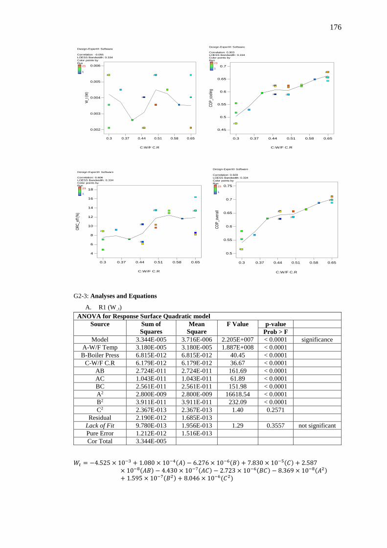
176
G2-3: Analyses and Equations
A. R1 (W_t)
ANOVA for Response Surface Quadratic model
Source Sum of
Squares
Mean
Square
F Value p-value
Prob > F
Model 3.344E-005 3.716E-006 2.205E+007 < 0.0001 significance
A-W/F Temp 3.180E-005 3.180E-005 1.887E+008 < 0.0001
B-Boiler Press 6.815E-012 6.815E-012 40.45 < 0.0001
C-W/F C.R 6.179E-012 6.179E-012 36.67 < 0.0001
AB 2.724E-011 2.724E-011 161.69 < 0.0001
AC 1.043E-011 1.043E-011 61.89 < 0.0001
BC 2.561E-011 2.561E-011 151.98 < 0.0001
A2 2.800E-009 2.800E-009 16618.54 < 0.0001
B2 3.911E-011 3.911E-011 232.09 < 0.0001
C2 2.367E-013 2.367E-013 1.40 0.2571
Residual 2.190E-012 1.685E-013
Lack of Fit 9.780E-013 1.956E-013 1.29 0.3557 not significant
Pure Error 1.212E-012 1.516E-013
Cor Total 3.344E-005
𝑊𝑡 = −4.525 × 10⁻³ + 1.080 × 10⁻⁴(𝐴) − 6.276 × 10⁻⁶(𝐵) + 7.830 × 10⁻⁵(𝐶) + 2.587× 10⁻⁸(𝐴𝐵) − 4.430 × 10⁻⁷(𝐴𝐶) − 2.723 × 10⁻⁶(𝐵𝐶) − 8.369 × 10⁻⁸(𝐴2)+ 1.595 × 10⁻⁷(𝐵2) + 8.046 × 10⁻⁶(𝐶2)
Design-Expert® Software
Correlation: -0.055
LOESS Bandwidth: 0.334
Color points by
Run
23
1
2
3
2
2
0.3 0.37 0.44 0.51 0.58 0.65
0.002
0.003
0.004
0.005
0.006
C:W/F C.R
W_t
(W)
Design-Expert® Software
Correlation: -0.055
LOESS Bandwidth: 0.334
Color points by
Run
23
1
2
3
2
2
0.3 0.37 0.44 0.51 0.58 0.65
0.002
0.003
0.004
0.005
0.006
C:W/F C.R
W_t
(W
)
Design-Expert® Software
Correlation: 0.903
LOESS Bandwidth: 0.334
Color points by
Run
23
1
2
2
2 2
2
2
0.3 0.37 0.44 0.51 0.58 0.65
0.45
0.5
0.55
0.6
0.65
0.7
C:W/F C.R
CO
P_co
olin
g
Design-Expert® Software
Correlation: 0.903
LOESS Bandwidth: 0.334
Color points by
Run
23
1
2
2
2 2
2
2
0.3 0.37 0.44 0.51 0.58 0.65
0.45
0.5
0.55
0.6
0.65
0.7
C:W/F C.R
CO
P_co
olin
g
Design-Expert® Software
Correlation: 0.606
LOESS Bandwidth: 0.334
Color points by
Run
23
1
2
2
2
2 2
0.3 0.37 0.44 0.51 0.58 0.65
4
6
8
10
12
14
16
18
C:W/F C.R
OR
C_e
ff (%
)
Design-Expert® Software
Correlation: 0.606
LOESS Bandwidth: 0.334
Color points by
Run
23
1
2
2
2
2 2
0.3 0.37 0.44 0.51 0.58 0.65
4
6
8
10
12
14
16
18
C:W/F C.R
OR
C_e
ff (%
)
Design-Expert® Software
Correlation: 0.929
LOESS Bandwidth: 0.334
Color points by
Run
23
1
2
2
22
2
0.3 0.37 0.44 0.51 0.58 0.65
0.5
0.55
0.6
0.65
0.7
0.75
C:W/F C.RC
OP
_ove
rall
Design-Expert® Software
Correlation: 0.929
LOESS Bandwidth: 0.334
Color points by
Run
23
1
2
2
22
2
0.3 0.37 0.44 0.51 0.58 0.65
0.5
0.55
0.6
0.65
0.7
0.75
C:W/F C.R
CO
P_o
vera
ll
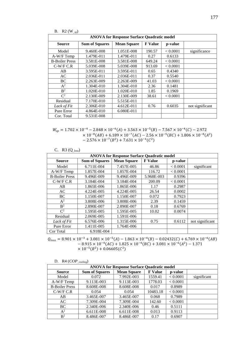
177
B. R2 (W_sp)
ANOVA for Response Surface Quadratic model
Source Sum of Squares Mean Square F Value p-value
Model 9.460E-008 1.051E-008 190.57 < 0.0001 significance
A-W/F Temp 1.479E-011 1.479E-011 0.27 0.6133
B-Boiler Press 3.581E-008 3.581E-008 649.24 < 0.0001
C-W/F C.R 5.039E-008 5.039E-008 913.69 < 0.0001
AB 3.595E-011 3.595E-011 0.65 0.4340
AC 2.036E-011 2.036E-011 0.37 0.5540
BC 2.263E-009 2.263E-009 41.03 < 0.0001
A2 1.304E-010 1.304E-010 2.36 0.1481
B2 1.020E-010 1.020E-010 1.85 0.1969
C2 2.130E-009 2.130E-009 38.61 < 0.0001
Residual 7.170E-010 5.515E-011
Lack of Fit 2.306E-010 4.612E-011 0.76 0.6035 not significant
Pure Error 4.864E-010 6.080E-011
Cor. Total 9.531E-008
𝑊𝑠𝑝 = 1.702 × 10⁻⁴ − 2.848 × 10⁻⁶(𝐴) + 3.563 × 10⁻⁵(𝐵) − 7.567 × 10⁻⁴(𝐶) − 2.972
× 10−8(𝐴𝐵) + 6.189 × 10⁻⁷(𝐴𝐶) − 2.56 × 10⁻⁵(𝐵𝐶) + 1.806 × 10⁻⁸(𝐴2)− 2.576 × 10⁻⁷(𝐵2) + 7.631 × 10⁻⁴(𝐶2)
C. R3 (Q_loss)
ANOVA for Response Surface Quadratic model
Source Sum of Squares Mean Square F Value p-value
Model 6.711E-004 7.457E-005 46.86 < 0.0001 significant
A-W/F Temp 1.857E-004 1.857E-004 116.72 < 0.0001
B-Boiler Press 9.496E-009 9.496E-009 5.968E-003 0.9396
C-W/F C.R 3.184E-004 3.184E-004 200.09 < 0.0001
AB 1.865E-006 1.865E-006 1.17 0.2987
AC 4.224E-005 4.224E-005 26.54 0.0002
BC 1.150E-007 1.150E-007 0.072 0.7923
A2 3.808E-006 3.808E-006 2.39 0.1459
B2 2.890E-007 2.890E-007 0.18 0.6769
C2 1.595E-005 1.595E-005 10.02 0.0074
Residual 2.069E-005 1.591E-006
Lack of Fit 6.576E-006 1.315E-006 0.75 0.6112 not significant
Pure Error 1.411E-005 1.764E-006
Cor Total 6.918E-004
𝑄𝑙𝑜𝑠𝑠 = 8.901 × 10⁻³ + 3.081 × 10⁻⁵(𝐴) − 1.863 × 10⁻⁴(𝐵) − 0.02432(𝐶) + 6.769 × 10⁻⁶(𝐴𝐵)− 8.915 × 10⁻⁴(𝐴𝐶) + 1.825 × 10⁻⁴(𝐵𝐶) + 3.081 × 10⁻⁶(𝐴2) − 1.371× 10⁻⁵(𝐵2) + 0.06605(𝐶2)
D. R4 (COP_cooling)
ANOVA for Response Surface Quadratic model
Source Sum of Squares Mean Square F Value p-value
Model 0.072 7.992E-003 1559.41 < 0.0001 significant
A-W/F Temp 9.113E-003 9.113E-003 1778.03 < 0.0001
B-Boiler Press 8.608E-008 8.608E-008 0.017 0.8989
C-W/F C.R 0.054 0.054 10483.18 < 0.0001
AB 3.465E-007 3.465E-007 0.068 0.7989
AC 7.309E-004 7.309E-004 142.60 < 0.0001
BC 2.340E-006 2.340E-006 0.46 0.5111
A2 6.611E-008 6.611E-008 0.013 0.9113
B2 8.486E-007 8.486E-007 0.17 0.6907

178
C2 1.383E-003 1.383E-003 269.81 < 0.0001
Residual 6.663E-005 5.125E-006
Lack of Fit 1.847E-005 3.694E-006 0.61 0.6937 not significant
Pure Error 4.816E-005 6.020E-006
Cor Total 0.072
𝐶𝑂𝑃𝑐𝑜𝑜𝑙𝑖𝑛𝑔 = 0.53197 − 3.379 × 10⁻³(𝐴) + 1.426 × 10⁻³(𝐵) + 0.709(𝐶) − 2.918 × 10⁻⁶(𝐴𝐵)
+ 3.708 × 10⁻³(𝐴𝐶) − 8.232 × 10⁻⁴(𝐵𝐶) + 4.066 × 10⁻⁷(𝐴2) − 2.349× 10⁻⁵(𝐵2) − 0.61498(𝐶2)
E. R5 (ORC_eff)
ANOVA for Response Surface Quadratic model
Source Sum of Squares Mean Square F Value p-value
Model 199.24 22.14 359.87 < 0.0001 significant
A-W/F Temp 111.77 111.77 1816.91 < 0.0001
B-Boiler Press 1.124E-003 1.124E-003 0.018 0.8945
C-W/F C.R 75.82 75.82 1232.57 < 0.0001
AB 0.028 0.028 0.46 0.5104
AC 5.58 5.58 90.76 < 0.0001
BC 0.040 0.040 0.66 0.4327
A2 1.16 1.16 18.80 0.0008
B2 0.060 0.060 0.98 0.3414
C2 0.19 0.19 3.01 0.1065
Residual 0.80 0.062
Lack of Fit 0.32 0.063 1.05 0.4501 not significant
Pure Error 0.48 0.060
Cor Total 200.04
𝑂𝑅𝐶𝑒𝑓𝑓 = −10.228 + +0.290(𝐴) − 0.226(𝐵) − 2.529(𝐶) + 8.321 × 10⁻⁴(𝐴𝐵) + 0.3241(𝐴𝐶)
− 0.108(𝐵𝐶) − 1.70110−3(𝐴2) + 6.246 × 10⁻³(𝐵2) − 7.1142(𝐶2)
F. R6 (COP_overall)
ANOVA for Response Surface Quadratic model
Source Sum of Squares Mean Square F Value p-value
Model 0.072 7.996E-003 579.26 < 0.0001 significant
A-W/F Temp 6.013E-003 6.013E-003 435.62 < 0.0001
B-Boiler Press 1.071E-005 1.071E-005 0.78 0.3945
C-W/F C.R 0.057 0.057 4157.66 < 0.0001
AB 2.262E-005 2.262E-005 1.64 0.2229
AC 4.825E-004 4.825E-004 34.95 < 0.0001
BC 2.078E-005 2.078E-005 1.51 0.2416
A2 9.449E-006 9.449E-006 0.68 0.4229
B2 3.366E-005 3.366E-005 2.44 0.1424
C2 1.774E-003 1.774E-003 128.52 < 0.0001
Residual 1.794E-004 1.380E-005
Lack of Fit 8.702E-005 1.740E-005 1.51 0.2885 not significant
Pure Error 9.243E-005 1.155E-005
Cor Total 0.072
𝐶𝑂𝑃𝑜𝑣𝑒𝑟𝑎𝑙𝑙 = 0.5955 − 3.921 × 10⁻³(𝐴) − 5.879 × 10⁻³(𝐵) + 0.885(𝐶) + 2.358 × 10⁻⁵(𝐴𝐵)+ 3.013 × 10⁻³(𝐴𝐶) − 2.453 × 10⁻³(𝐵𝐶) + 4.862 × 10⁻⁶(𝐴2) + 1.480× 10⁻⁴(𝐵2) − 0.696(𝐶2)

179
G2-3: Diagnostics and Model Graphs
A. R1 (W_t)
B. R2 (W_sp)
Design-Expert® Software
W_t
Color points by value of
W_t:
0.0054234
0.0021162
Actual
Pred
icte
d
Predicted vs. Actual
2.00E-03
3.00E-03
4.00E-03
5.00E-03
6.00E-03
0.002 0.003 0.004 0.005 0.006
Design-Expert® Software
W_t
Color points by value of
W_t:
0.0054234
0.0021162
Actual
Pred
icte
d
Predicted vs. Actual
2.00E-03
3.00E-03
4.00E-03
5.00E-03
6.00E-03
0.002 0.003 0.004 0.005 0.006
Design-Expert® Software
W_t
Color points by value of
W_t:
0.0054234
0.0021162
Predicted
Exte
rnal
ly S
tude
ntiz
ed R
esid
uals
Residuals vs. Predicted
-4.00
-2.00
0.00
2.00
4.00
0.002 0.003 0.004 0.005 0.006
3.88354
-3.88354
0
Design-Expert® Software
W_t
Color points by value of
W_t:
0.0054234
0.0021162
Predicted
Exte
rnal
ly S
tude
ntiz
ed R
esid
uals
Residuals vs. Predicted
-4.00
-2.00
0.00
2.00
4.00
0.002 0.003 0.004 0.005 0.006
3.88354
-3.88354
0
Design-Expert® Software
W_t
Lambda
Current = 1
Best = 1.01
Low C.I. = 0.95
High C.I. = 1.06
Recommend transform:
None
(Lambda = 1)
Lambda
Ln(R
esid
ualS
S)
Box-Cox Plot for Power Transforms
-28
-26
-24
-22
-20
-18
-16
-14
-3 -2 -1 0 1 2 3
-26.7106
Design-Expert® Software
W_t
Lambda
Current = 1
Best = 1.01
Low C.I. = 0.95
High C.I. = 1.06
Recommend transform:
None
(Lambda = 1)
Lambda
Ln(R
esid
ualS
S)
Box-Cox Plot for Power Transforms
-28
-26
-24
-22
-20
-18
-16
-14
-3 -2 -1 0 1 2 3
-26.7106
Design-Expert® Software
Factor Coding: Actual
W_t (W)
0.0054234
0.0021162
X1 = A: W/F Temp
X2 = B: Boiler Press
Actual Factor
C: W/F C.R = 0.475
12 13
14 15
16 17
18 19
20 21
65 72
79 86
93 100
0.002
0.003
0.004
0.005
0.006
W_
t (W
)
A: W/F Temp (C)B: Boiler Press (Bar)
Design-Expert® Software
Factor Coding: Actual
W_t (W)
0.0054234
0.0021162
X1 = A: W/F Temp
X2 = B: Boiler Press
Actual Factor
C: W/F C.R = 0.475
12 13
14 15
16 17
18 19
20 21
65 72
79 86
93 100
0.002
0.003
0.004
0.005
0.006
W_
t (W
)
A: W/F Temp (C)B: Boiler Press (Bar)
Design-Expert® Software
W_sp
Color points by value of
W_sp:
0.0003492
8.48E-005
Actual
Pre
dict
ed
Predicted vs. Actual
5.00E-05
1.00E-04
1.50E-04
2.00E-04
2.50E-04
3.00E-04
3.50E-04
5E-005
0.0001
0.00015
0.0002
0.00025
0.0003
0.00035
Design-Expert® Software
W_sp
Color points by value of
W_sp:
0.0003492
8.48E-005
Actual
Pre
dict
ed
Predicted vs. Actual
5.00E-05
1.00E-04
1.50E-04
2.00E-04
2.50E-04
3.00E-04
3.50E-045E
-005
0.0001
0.00015
0.0002
0.00025
0.0003
0.00035
Design-Expert® Software
W_sp
Color points by value of
W_sp:
0.0003492
8.48E-005
Predicted
Exte
rnal
ly S
tude
ntiz
ed R
esid
uals
Residuals vs. Predicted
-4.00
-2.00
0.00
2.00
4.00
5E-005
0.0001
0.00015
0.0002
0.00025
0.0003
0.00035
3.88354
-3.88354
0
Design-Expert® Software
W_sp
Color points by value of
W_sp:
0.0003492
8.48E-005
Predicted
Exte
rnal
ly S
tude
ntiz
ed R
esid
uals
Residuals vs. Predicted
-4.00
-2.00
0.00
2.00
4.00
5E-005
0.0001
0.00015
0.0002
0.00025
0.0003
0.00035
3.88354
-3.88354
0
Design-Expert® Software
W_sp
Lambda
Current = 1
Best = 0.2
Low C.I. = -1.61
High C.I. = 1.38
Recommend transform:
None
(Lambda = 1)
Lambda
Ln(R
esid
ualS
S)
Box-Cox Plot for Power Transforms
-21.5
-21
-20.5
-20
-19.5
-19
-3 -2 -1 0 1 2 3
-20.8714
Design-Expert® Software
W_sp
Lambda
Current = 1
Best = 0.2
Low C.I. = -1.61
High C.I. = 1.38
Recommend transform:
None
(Lambda = 1)
Lambda
Ln(R
esid
ualS
S)
Box-Cox Plot for Power Transforms
-21.5
-21
-20.5
-20
-19.5
-19
-3 -2 -1 0 1 2 3
-20.8714
Design-Expert® Software
Factor Coding: Actual
W_sp (W)
0.0003492
8.48E-005
X1 = A: W/F Temp
X2 = B: Boiler Press
Actual Factor
C: W/F C.R = 0.475
12 13
14 15
16 17
18 19
20 21
65 72
79 86
93 100
5E-005
0.0001
0.00015
0.0002
0.00025
0.0003
0.00035
W_s
p (W
)
A: W/F Temp (C)B: Boiler Press (Bar)
Design-Expert® Software
Factor Coding: Actual
W_sp (W)
0.0003492
8.48E-005
X1 = A: W/F Temp
X2 = B: Boiler Press
Actual Factor
C: W/F C.R = 0.475
12 13
14 15
16 17
18 19
20 21
65 72
79 86
93 100
5E-005
0.0001
0.00015
0.0002
0.00025
0.0003
0.00035
W_s
p (W
)
A: W/F Temp (C)B: Boiler Press (Bar)
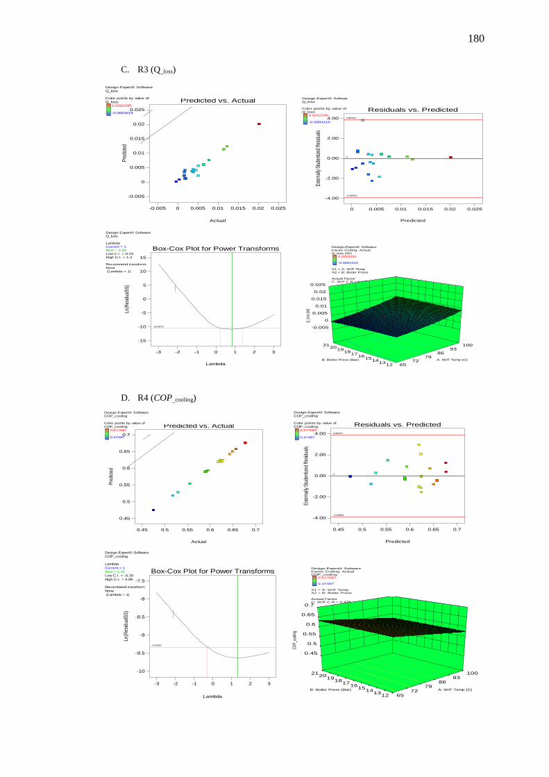
180
C. R3 (Q_loss)
D. R4 (COP_cooling)
Design-Expert® Software
Q_loss
Color points by value of
Q_loss:
0.0202295
-0.0003419
Actual
Pre
dict
ed
Predicted vs. Actual
-0.005
0
0.005
0.01
0.015
0.02
0.025
-0.005 0 0.005 0.01 0.015 0.02 0.025
Design-Expert® Software
Q_loss
Color points by value of
Q_loss:
0.0202295
-0.0003419
Actual
Pre
dict
ed
Predicted vs. Actual
-0.005
0
0.005
0.01
0.015
0.02
0.025
-0.005 0 0.005 0.01 0.015 0.02 0.025
Design-Expert® Software
Q_loss
Color points by value of
Q_loss:
0.0202295
-0.0003419
Predicted
Exte
rnal
ly St
uden
tized
Res
idua
ls
Residuals vs. Predicted
-4.00
-2.00
0.00
2.00
4.00
0 0.005 0.01 0.015 0.02 0.025
3.88354
-3.88354
0
Design-Expert® Software
Q_loss
Color points by value of
Q_loss:
0.0202295
-0.0003419
Predicted
Exte
rnal
ly St
uden
tized
Res
idua
ls
Residuals vs. Predicted
-4.00
-2.00
0.00
2.00
4.00
0 0.005 0.01 0.015 0.02 0.025
3.88354
-3.88354
0
Design-Expert® Software
Q_loss
Lambda
Current = 1
Best = 0.83
Low C.I. = 0.23
High C.I. = 1.4
Recommend transform:
None
(Lambda = 1)
k = 0.00037609
(used to make
response values
positive)
Lambda
Ln(R
esid
ualS
S)
Box-Cox Plot for Power Transforms
-15
-10
-5
0
5
10
15
-3 -2 -1 0 1 2 3
-10.5079
Design-Expert® Software
Q_loss
Lambda
Current = 1
Best = 0.83
Low C.I. = 0.23
High C.I. = 1.4
Recommend transform:
None
(Lambda = 1)
k = 0.00037609
(used to make
response values
positive)
Lambda
Ln(R
esid
ualS
S)
Box-Cox Plot for Power Transforms
-15
-10
-5
0
5
10
15
-3 -2 -1 0 1 2 3
-10.5079
Design-Expert® Software
Factor Coding: Actual
Q_loss (W)
0.0202295
-0.0003419
X1 = A: W/F Temp
X2 = B: Boiler Press
Actual Factor
C: W/F C.R = 0.475
12 13
14 15
16 17
18 19
20 21
65 72
79 86
93 100
-0.005
0
0.005
0.01
0.015
0.02
0.025
Q_l
oss
(W)
A: W/F Temp (C)B: Boiler Press (Bar)
Design-Expert® Software
Factor Coding: Actual
Q_loss (W)
0.0202295
-0.0003419
X1 = A: W/F Temp
X2 = B: Boiler Press
Actual Factor
C: W/F C.R = 0.475
12 13
14 15
16 17
18 19
20 21
65 72
79 86
93 100
-0.005
0
0.005
0.01
0.015
0.02
0.025
Q_l
oss
(W)
A: W/F Temp (C)B: Boiler Press (Bar)
Design-Expert® Software
COP_cooling
Color points by value of
COP_cooling:
0.677087
0.47497
Actual
Pre
dict
ed
Predicted vs. Actual
0.45
0.5
0.55
0.6
0.65
0.7
0.45 0.5 0.55 0.6 0.65 0.7
Design-Expert® Software
COP_cooling
Color points by value of
COP_cooling:
0.677087
0.47497
Actual
Pre
dict
ed
Predicted vs. Actual
0.45
0.5
0.55
0.6
0.65
0.7
0.45 0.5 0.55 0.6 0.65 0.7
Design-Expert® Software
COP_cooling
Color points by value of
COP_cooling:
0.677087
0.47497
Predicted
Exte
rnal
ly S
tude
ntiz
ed R
esid
uals
Residuals vs. Predicted
-4.00
-2.00
0.00
2.00
4.00
0.45 0.5 0.55 0.6 0.65 0.7
3.88354
-3.88354
0
Design-Expert® Software
COP_cooling
Color points by value of
COP_cooling:
0.677087
0.47497
Predicted
Exte
rnal
ly S
tude
ntiz
ed R
esid
uals
Residuals vs. Predicted
-4.00
-2.00
0.00
2.00
4.00
0.45 0.5 0.55 0.6 0.65 0.7
3.88354
-3.88354
0
Design-Expert® Software
COP_cooling
Lambda
Current = 1
Best = 1.32
Low C.I. = -0.29
High C.I. = 4.08
Recommend transform:
None
(Lambda = 1)
Lambda
Ln(R
esid
ualS
S)
Box-Cox Plot for Power Transforms
-10
-9.5
-9
-8.5
-8
-7.5
-3 -2 -1 0 1 2 3
-9.33032
Design-Expert® Software
COP_cooling
Lambda
Current = 1
Best = 1.32
Low C.I. = -0.29
High C.I. = 4.08
Recommend transform:
None
(Lambda = 1)
Lambda
Ln(R
esid
ualS
S)
Box-Cox Plot for Power Transforms
-10
-9.5
-9
-8.5
-8
-7.5
-3 -2 -1 0 1 2 3
-9.33032
Design-Expert® Software
Factor Coding: Actual
COP_cooling
0.677087
0.47497
X1 = A: W/F Temp
X2 = B: Boiler Press
Actual Factor
C: W/F C.R = 0.475
12 13
14 15
16 17
18 19
20 21
65 72
79 86
93 100
0.45
0.5
0.55
0.6
0.65
0.7
COP_
cooli
ng
A: W/F Temp (C)B: Boiler Press (Bar)
Design-Expert® Software
Factor Coding: Actual
COP_cooling
0.677087
0.47497
X1 = A: W/F Temp
X2 = B: Boiler Press
Actual Factor
C: W/F C.R = 0.475
12 13
14 15
16 17
18 19
20 21
65 72
79 86
93 100
0.45
0.5
0.55
0.6
0.65
0.7
CO
P_co
olin
g
A: W/F Temp (C)B: Boiler Press (Bar)
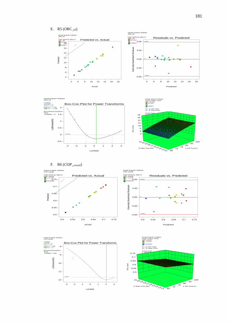
181
E. R5 (ORC_eff)
F. R6 (COP_overall)
Design-Expert® Software
ORC_eff
Color points by value of
ORC_eff:
16.3385
4.85611
Actual
Pre
dict
ed
Predicted vs. Actual
4
6
8
10
12
14
16
18
4 6 8 10 12 14 16 18
Design-Expert® Software
ORC_eff
Color points by value of
ORC_eff:
16.3385
4.85611
Actual
Pre
dict
ed
Predicted vs. Actual
4
6
8
10
12
14
16
18
4 6 8 10 12 14 16 18
Design-Expert® Software
ORC_eff
Color points by value of
ORC_eff:
16.3385
4.85611
Predicted
Exte
rnal
ly S
tude
ntiz
ed R
esid
uals
Residuals vs. Predicted
-4.00
-2.00
0.00
2.00
4.00
4 6 8 10 12 14 16 18
3.88354
-3.88354
0
Design-Expert® Software
ORC_eff
Color points by value of
ORC_eff:
16.3385
4.85611
Predicted
Exte
rnal
ly S
tude
ntiz
ed R
esid
uals
Residuals vs. Predicted
-4.00
-2.00
0.00
2.00
4.00
4 6 8 10 12 14 16 18
3.88354
-3.88354
0
Design-Expert® Software
ORC_eff
Lambda
Current = 1
Best = 0.21
Low C.I. = -0.9
High C.I. = 1.99
Recommend transform:
None
(Lambda = 1)
Lambda
Ln(R
esid
ualS
S)
Box-Cox Plot for Power Transforms
-0.5
0
0.5
1
1.5
2
-3 -2 -1 0 1 2 3
-0.013915
Design-Expert® Software
ORC_eff
Lambda
Current = 1
Best = 0.21
Low C.I. = -0.9
High C.I. = 1.99
Recommend transform:
None
(Lambda = 1)
Lambda
Ln(R
esid
ualS
S)
Box-Cox Plot for Power Transforms
-0.5
0
0.5
1
1.5
2
-3 -2 -1 0 1 2 3
-0.013915
Design-Expert® Software
Factor Coding: Actual
ORC_eff (%)
16.3385
4.85611
X1 = A: W/F Temp
X2 = B: Boiler Press
Actual Factor
C: W/F C.R = 0.475
12 13
14 15
16 17
18 19
20 21
65 72
79 86
93 100
4
6
8
10
12
14
16
18
OR
C_e
ff (%
)
A: W/F Temp (C)B: Boiler Press (Bar)
Design-Expert® Software
Factor Coding: Actual
ORC_eff (%)
16.3385
4.85611
X1 = A: W/F Temp
X2 = B: Boiler Press
Actual Factor
C: W/F C.R = 0.475
12 13
14 15
16 17
18 19
20 21
65 72
79 86
93 100
4
6
8
10
12
14
16
18
OR
C_e
ff (%
)
A: W/F Temp (C)B: Boiler Press (Bar)
Design-Expert® Software
COP_overall
Color points by value of
COP_overall:
0.711296
0.516106
Actual
Pred
icte
d
Predicted vs. Actual
0.5
0.55
0.6
0.65
0.7
0.75
0.5 0.55 0.6 0.65 0.7 0.75
Design-Expert® Software
COP_overall
Color points by value of
COP_overall:
0.711296
0.516106
Actual
Pred
icte
d
Predicted vs. Actual
0.5
0.55
0.6
0.65
0.7
0.75
0.5 0.55 0.6 0.65 0.7 0.75
Design-Expert® Software
COP_overall
Color points by value of
COP_overall:
0.711296
0.516106
Predicted
Exte
rnal
ly S
tude
ntiz
ed R
esid
uals
Residuals vs. Predicted
-4.00
-2.00
0.00
2.00
4.00
0.5 0.55 0.6 0.65 0.7 0.75
3.88354
-3.88354
0
Design-Expert® Software
COP_overall
Color points by value of
COP_overall:
0.711296
0.516106
Predicted
Exte
rnal
ly S
tude
ntiz
ed R
esid
uals
Residuals vs. Predicted
-4.00
-2.00
0.00
2.00
4.00
0.5 0.55 0.6 0.65 0.7 0.75
3.88354
-3.88354
0
Design-Expert® Software
COP_overall
Lambda
Current = 1
Best = 2.05
Low C.I. = 1.29
High C.I. = 3
Recommend transform:
Power
(Lambda = 2.05)
Lambda
Ln(R
esid
ualS
S)
Box-Cox Plot for Power Transforms
-12
-11
-10
-9
-8
-3 -2 -1 0 1 2 3
-11.6884
Design-Expert® Software
COP_overall
Lambda
Current = 1
Best = 2.05
Low C.I. = 1.29
High C.I. = 3
Recommend transform:
Power
(Lambda = 2.05)
Lambda
Ln(R
esid
ualS
S)
Box-Cox Plot for Power Transforms
-12
-11
-10
-9
-8
-3 -2 -1 0 1 2 3
-11.6884
Design-Expert® Software
Factor Coding: Actual
COP_overall
0.711296
0.516106
X1 = A: W/F Temp
X2 = B: Boiler Press
Actual Factor
C: W/F C.R = 0.475
12 13
14 15
16 17
18 19
20 21
65 72
79 86
93 100
0.5
0.55
0.6
0.65
0.7
0.75
CO
P_ov
eral
l
A: W/F Temp (C)B: Boiler Press (Bar)
Design-Expert® Software
Factor Coding: Actual
COP_overall
0.711296
0.516106
X1 = A: W/F Temp
X2 = B: Boiler Press
Actual Factor
C: W/F C.R = 0.475
12 13
14 15
16 17
18 19
20 21
65 72
79 86
93 100
0.5
0.55
0.6
0.65
0.7
0.75
CO
P_ov
eral
l
A: W/F Temp (C)B: Boiler Press (Bar)

182
APPENDIX H
PROJECT INFORMATION ON RETScreen
H1: Project Information and Specifications
1. Proposed case (0.05kW Capacity)
i. Base load cooling system
Technology Absorption
Fuel type User-defined fuel
Fuel rate RM /kJ 0.000
Capacity kW 0.05 104.7 %
COP- seasonal 0.65
Cooling delivered MWh 0.44 60.5 %
ii. Base load power system
Technology Solar thermal power
Power capacity kW 0.0045 13.5 %
Model
Capacity factor % 20.0 %
Electricity delivered to load MWh 0.0026 5.7 %
Electricity exported to grid MWh 0
iii. Operating strategy - base load power system
Electricity rate - base case RM /MWh 218.00
Fuel rate - proposed case power system RM /MWh 0.00
Electricity export rate RM /MWh 218.00
Electricity rate - proposed case RM /MWh 218.00
iv. Proposed case system characteristics
Power Unit Estimate %
Base load power system
Technology Solar thermal power
Operating strategy Full power capacity output
Capacity kW 0 13.5 %
Electricity delivered to load MWh 0 5.7 %
Electricity exported to grid MWh 0
Cooling
Base load cooling system
Technology Absorption
Fuel type User-defined fuel
Capacity kW 0 104.7 %
Cooling delivered MWh 0 60.5 %
2. Proposed case (1.76 kW Capacity)
i. Base load cooling system
Technology Absorption
Fuel type User-defined fuel
Fuel rate MYR/kJ
Capacity kW 1.76 87.5 %
COP- seasonal 0.60
Cooling delivered MWh 15 50.6 %
ii. Base load power system
Technology Solar thermal power
Power capacity kW 0.142 11.2 %
Capacity factor % 20.0 %
Electricity delivered to load MWh 0 7.1 %
Electricity exported to grid MWh 0
iii. Operating strategy - base load power system

183
Electricity rate - base case RM /MWh 218.00
Fuel rate - proposed case power system RM /MWh 0.00
Electricity export rate RM /MWh 218.00
Electricity rate - proposed case RM /MWh 218.00
iv. Proposed case system characteristics
Power Unit Estimate %
Base load power system
Technology Solar thermal power
Operating strategy Full power capacity output
Capacity kW 0.142 11.2 %
Electricity delivered to load MWh 7.1 %
Electricity exported to grid MWh 0
Cooling
Base load cooling system
Technology Absorption
Fuel type User-defined fuel
Capacity kW 2 87.5 %
Cooling delivered MWh 15 50.6 %
3. Proposed case (3.5 kW Capacity)
i. Base load cooling system
Technology Absorption
Fuel type User-defined fuel
Fuel rate RM /kJ
Capacity kW 3.5 79.1 %
COP - seasonal 0.65
Cooling delivered MWh 31 45.8 %
ii. Base load power system
Technology Solar thermal power
Power capacity kW 0.283 13.1 %
Capacity factor % 20.0 %
Electricity delivered to load MWh 11.6 %
Electricity exported to grid MWh 0
iii. Operating strategy - base load power system
Electricity rate - base case RM /MWh 218.00
Fuel rate - proposed case power system RM /MWh 0.00
Electricity export rate RM /MWh 218.00
Electricity rate - proposed case RM /MWh 218.00
iv. Proposed case system characteristics
Power Unit Estimate %
Base load power system
Technology Solar thermal power
Operating strategy Full power capacity output
Capacity kW 0.283 13.1 %
Electricity delivered to load MWh 0 11.6 %
Electricity exported to grid MWh 0
Cooling
Base load cooling system
Technology Absorption
Fuel type User-defined fuel
Capacity kW 4 79.1 %
Cooling delivered MWh 31 45.8 %
4. Proposed case (7.0 kW Capacity)
i. Base load cooling system
Technology Absorption
Fuel type User-defined fuel (Solar)
Fuel rate RM /kJ
Capacity kW 7.0 79.1 %
COP - seasonal 0.65
Cooling delivered MWh 61 45.8 %
ii. Base load power system
Technology Solar thermal power
Power capacity kW 0.565 14.8 %
Capacity factor % 20.0 %
Electricity delivered to load MWh 1 12.0 %
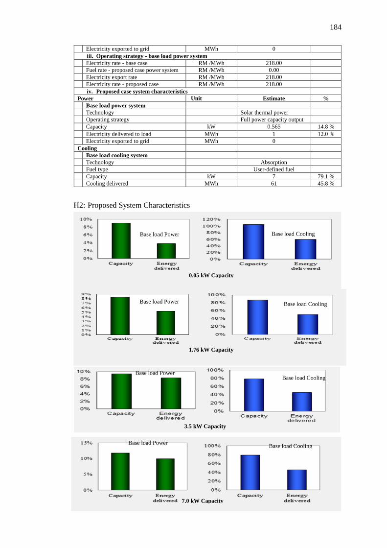
184
Electricity exported to grid MWh 0
iii. Operating strategy - base load power system
Electricity rate - base case RM /MWh 218.00
Fuel rate - proposed case power system RM /MWh 0.00
Electricity export rate RM /MWh 218.00
Electricity rate - proposed case RM /MWh 218.00
iv. Proposed case system characteristics
Power Unit Estimate %
Base load power system
Technology Solar thermal power
Operating strategy Full power capacity output
Capacity kW 0.565 14.8 %
Electricity delivered to load MWh 1 12.0 %
Electricity exported to grid MWh 0
Cooling
Base load cooling system
Technology Absorption
Fuel type User-defined fuel
Capacity kW 7 79.1 %
Cooling delivered MWh 61 45.8 %
H2: Proposed System Characteristics
1.76 kW Capacity
Base load Power Base load Cooling
Base load Power Base load Cooling
3.5 kW Capacity
Base load Power Base load Cooling
0.05 kW Capacity
7.0 kW Capacity
Base load Power Base load Cooling
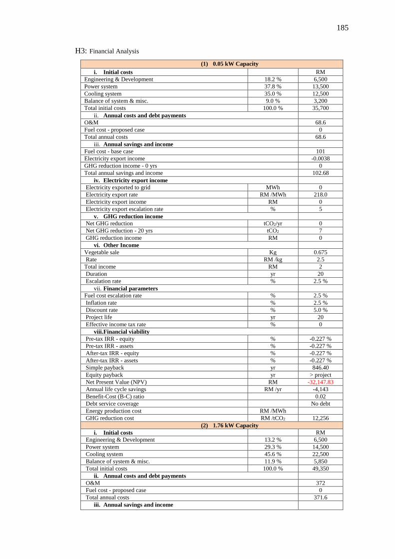
185
H3: Financial Analysis
(1) 0.05 kW Capacity
i. Initial costs RM
Engineering & Development 18.2 % 6,500
Power system 37.8 % 13,500
Cooling system 35.0 % 12,500
Balance of system & misc. 9.0 % 3,200
Total initial costs 100.0 % 35,700
ii. Annual costs and debt payments
O&M 68.6
Fuel cost - proposed case 0
Total annual costs 68.6
iii. Annual savings and income
Fuel cost - base case 101
Electricity export income -0.0038
GHG reduction income - 0 yrs 0
Total annual savings and income 102.68
iv. Electricity export income
Electricity exported to grid MWh 0
Electricity export rate RM /MWh 218.0
Electricity export income RM 0
Electricity export escalation rate % 5
v. GHG reduction income
Net GHG reduction tCO2/yr 0
Net GHG reduction - 20 yrs tCO2 7
GHG reduction income RM 0
vi. Other Income
Vegetable sale Kg 0.675
Rate RM /kg 2.5
Total income RM 2
Duration yr 20
Escalation rate % 2.5 %
vii. Financial parameters
Fuel cost escalation rate % 2.5 %
Inflation rate % 2.5 %
Discount rate % 5.0 %
Project life yr 20
Effective income tax rate % 0
viii. Financial viability
Pre-tax IRR - equity % -0.227 %
Pre-tax IRR - assets % -0.227 %
After-tax IRR - equity % -0.227 %
After-tax IRR - assets % -0.227 %
Simple payback yr 846.40
Equity payback yr > project
Net Present Value (NPV) RM -32,147.83
Annual life cycle savings RM /yr -4,143
Benefit-Cost (B-C) ratio 0.02
Debt service coverage No debt
Energy production cost RM /MWh
GHG reduction cost RM /tCO2 12,256
(2) 1.76 kW Capacity
i. Initial costs RM
Engineering & Development 13.2 % 6,500
Power system 29.3 % 14,500
Cooling system 45.6 % 22,500
Balance of system & misc. 11.9 % 5,850
Total initial costs 100.0 % 49,350
ii. Annual costs and debt payments
O&M 372
Fuel cost - proposed case 0
Total annual costs 371.6
iii. Annual savings and income

186
Fuel cost - base case 3,531
Electricity export income 0.0051
GHG reduction income - 0 yrs 0
Total annual savings and income 3,591.76
iv. Electricity export income
Electricity exported to grid MWh 0
Electricity export rate RM /MWh 218.00
Electricity export income RM 0
Electricity export escalation rate % 5
v. GHG reduction income
Net GHG reduction tCO2/yr 12
Net GHG reduction - 20 yrs tCO2 236
GHG reduction income RM 0
vi. Other income
Vegetable sales Kg 24.3
Rate RM /kg 2.5
Total income RM 60.75
Duration yr 20
Escalation rate % 2.5 %
vii. Financial parameters
Fuel cost escalation rate % 2.5 %
Inflation rate % 2.5 %
Discount rate % 5.0 %
Project life yr 20
Effective income tax rate % 0
viii. Financial viability
Pre-tax IRR - equity % 5.0 %
Pre-tax IRR - assets % 5.0 %
After-tax IRR - equity % 5.0 %
After-tax IRR - assets % 5.0 %
Simple payback yr 15.3
Equity payback yr 12.38
Net Present Value (NPV) RM -1229.57
Annual life cycle savings RM /yr 1337
Benefit-Cost (B-C) ratio 1.34
Debt service coverage No debt
Energy production cost RM /MWh
GHG reduction cost RM /tCO2 (113)
(3) 3.5 kW Capacity
i. Initial costs RM
Engineering and Development 10.2 % 6,500
Power system 32.3 % 20,500
Cooling system 39.4 % 25,000
Balance of system & misc. 18.1 % 11,525
Total initial costs 100.0 % 63,525
ii. Annual costs and debt payments
O&M 568.2
Fuel cost - proposed case 0
Total annual costs 568.2
iii. Annual savings and income
Fuel cost - base case 7,018
Electricity export income 0.019
GHG reduction income - 0 yrs 0
Customer premium income (rebate) 0
Total annual savings and income 7,139
iv. Electricity export income
Electricity exported to grid MWh 0
Electricity export rate RM /MWh 218.00
Electricity export income RM 0
Electricity export escalation rate % 5
v. GHG reduction income
Net GHG reduction tCO2/yr 23
Net GHG reduction - 20 yrs tCO2 468
Net GHG reduction - 0 yrs tCO2 0

187
vi. Other income
Vegetable Sales Kg 48.6
Rate RM /kg 2.5
Total RM 122
Duration yr 20
Escalation rate % 2.5 %
vii. Financial parameters
Fuel cost escalation rate % 2.5 %
Inflation rate % 2.5 %
Discount rate % 5.0 %
Project life yr 20
Effective income tax rate % 0
viii. Financial viability
Pre-tax IRR - equity % 10 %
Pre-tax IRR - assets % 10 %
Simple payback yr 9.7
Equity payback yr 7.93
Net Present Value (NPV) RM 32,902.98
Annual life cycle savings RM /yr 5,645
Benefit-Cost (B-C) ratio 2.11
Debt service coverage No debt
Energy production cost RM /MWh
GHG reduction cost RM/tCO2 (241)
(4) 7 kW Capacity
i. Initial costs RM
Engineering & Development 6.7 % 6,500
Power system 25.6 % 25,000
Cooling system 50.2 % 49,000
Balance of system & misc. 17.6 % 17,150
Total initial costs 100.0 % 97,650
ii. Annual costs and debt payments
O&M 873.9
Fuel cost - proposed case 0
Total annual costs 873.9
iii. Annual savings and income
Fuel cost - base case 13,897
Electricity export income 0
GHG reduction income - 0 yrs 0
Total annual savings and income 14,141
iv. Electricity export income
Electricity exported to grid MWh 0
Electricity export rate RM /MWh 218.00
Electricity export income RM 0.051
Electricity export escalation rate %
v. GHG reduction income
Net GHG reduction tCO2/yr 46
Net GHG reduction - 20 yrs tCO2 927
GHG reduction credit rate RM/tCO2
GHG reduction income RM 0
vi. Other income
Vegetables kg 97.2
Rate RM/kg 2.5
Total RM 243
Duration yr 20
Escalation rate % 2.5 %
vii. Financial parameters
Fuel cost escalation rate % 2.5 %
Inflation rate % 2.5 %
Discount rate % 10.0 %
Project life yr 20
Effective income tax rate % 0
viii. Financial viability
Pre-tax IRR - equity % 14.0 %
Pre-tax IRR - assets % 14.0 %
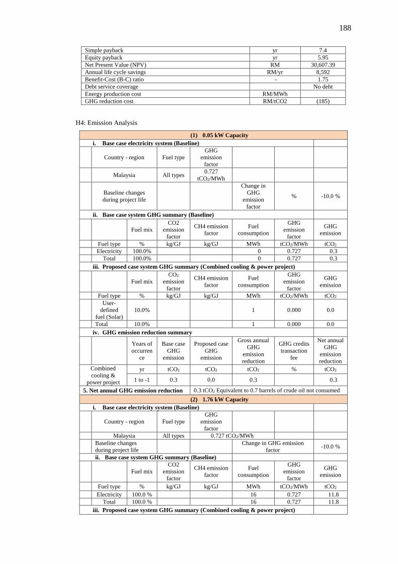
188
Simple payback yr 7.4
Equity payback yr 5.95
Net Present Value (NPV) RM 30,607.39
Annual life cycle savings RM/yr 8,592
Benefit-Cost (B-C) ratio - 1.75
Debt service coverage No debt
Energy production cost RM/MWh
GHG reduction cost RM/tCO2 (185)
H4: Emission Analysis
(1) 0.05 kW Capacity
i. Base case electricity system (Baseline)
Country - region Fuel type
GHG
emission
factor
Malaysia All types 0.727
tCO2/MWh
Baseline changes
during project life
Change in
GHG
emission
factor
% -10.0 %
ii. Base case system GHG summary (Baseline)
Fuel mix
CO2
emission
factor
CH4 emission
factor
Fuel
consumption
GHG
emission
factor
GHG
emission
Fuel type % kg/GJ kg/GJ MWh tCO2/MWh tCO2
Electricity 100.0% 0 0.727 0.3
Total 100.0% 0 0.727 0.3
iii. Proposed case system GHG summary (Combined cooling & power project)
Fuel mix
CO2
emission
factor
CH4 emission
factor
Fuel
consumption
GHG
emission
factor
GHG
emission
Fuel type % kg/GJ kg/GJ MWh tCO2/MWh tCO2
User-
defined
fuel (Solar)
10.0% 1 0.000 0.0
Total 10.0% 1 0.000 0.0
iv. GHG emission reduction summary
Years of
occurren
ce
Base case
GHG
emission
Proposed case
GHG
emission
Gross annual
GHG
emission
reduction
GHG credits
transaction
fee
Net annual
GHG
emission
reduction
Combined
cooling &
power project
yr tCO2 tCO2 tCO2 % tCO2
1 to -1 0.3 0.0 0.3 0.3
5. Net annual GHG emission reduction 0.3 tCO2 Equivalent to 0.7 barrels of crude oil not consumed
(2) 1.76 kW Capacity
i. Base case electricity system (Baseline)
Country - region Fuel type
GHG
emission
factor
Malaysia All types 0.727 tCO2/MWh
Baseline changes
during project life
Change in GHG emission
factor -10.0 %
ii. Base case system GHG summary (Baseline)
Fuel mix
CO2
emission
factor
CH4 emission
factor
Fuel
consumption
GHG
emission
factor
GHG
emission
Fuel type % kg/GJ kg/GJ MWh tCO2/MWh tCO2
Electricity 100.0 % 16 0.727 11.8
Total 100.0 % 16 0.727 11.8
iii. Proposed case system GHG summary (Combined cooling & power project)

189
Fuel mix
CO2
emission
factor
CH4 emission
factor
Fuel
consumption
GHG
emission
factor
GHG
emission
Fuel type % kg/GJ kg/GJ MWh tCO2/MWh tCO2
User-
defined
fuel (Solar)
100 % 28 0.000 0.0
Total 100.0 % 28 0.000 0.0
iv. GHG emission reduction summary
Years of
occurren
ce
Base case
GHG
emission
Proposed case
GHG
emission
Gross annual
GHG
emission
reduction
GHG credits
transaction
fee
Net annual
GHG
emission
reduction
Combined
cooling &
power project
yr tCO2 tCO2 tCO2 % tCO2
1 to -1 11.8 0.0 11.8 11.8
v. Net annual GHG emission reduction 11.8 tCO2, equivalent to 27.4 Barrels of crude oil not
consumed
(3) 3.5 kW Capacity
i. Base case electricity system (Baseline)
Country - region Fuel type GHG
emission
factor
Malaysia All types 0.727 tCO2/MWh
Baseline changes
during project life
Change in GHG emission
factor
-10.0%
ii. Base case system GHG summary (Baseline)
Fuel mix CO2
emission
factor
CH4 emission
factor
Fuel
consumption
GHG
emission
factor
GHG
emission
Fuel type % kg/GJ kg/GJ MWh tCO2/MWh tCO2
Electricity 100.0 % 32 0.727 23.4
Total 100.0 % 32 0.727 23.4
iii. Proposed case system GHG summary (Combined cooling & power project)
Fuel mix CO2
emission
factor
CH4 emission
factor
Fuel
consumption
GHG
emission
factor
GHG
emission
Fuel type % kg/GJ kg/GJ MWh tCO2/MWh tCO2
User-
defined
fuel (Solar)
100 % 47 0.000 0.0
Total 100.0 % 48 0.000 0.0
iv. GHG emission reduction summary
Years of
occurren
ce
Base case
GHG
emission
Proposed case
GHG
emission
Gross annual
GHG
emission
reduction
GHG credits
transaction
fee
Net annual
GHG
emission
reduction
Combined
cooling &
power project
yr tCO2 tCO2 tCO2 % tCO2
1 to -1 23.4 0.0 23.4
23.4
v. Net annual GHG emission reduction 23.4tCO2 Equivalent to 54.4 Barrels of crude oil not
consumed
(4) 7.0 kW Capacity
i. Base case electricity system (Baseline)
Country - region Fuel type
GHG
emission
factor
Malaysia All types 0.727
tCO2/MWh
Baseline changes
during project life
Change in
GHG
emission
factor
% -10.0 %
ii. Base case system GHG summary (Baseline)
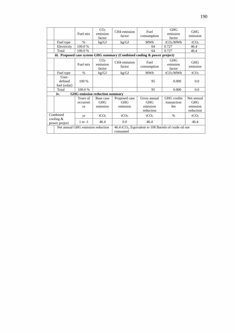
190
Fuel mix
CO2
emission
factor
CH4 emission
factor
Fuel
consumption
GHG
emission
factor
GHG
emission
Fuel type % kg/GJ kg/GJ MWh tCO2/MWh tCO2
Electricity 100.0 % 64 0.727 46.4
Total 100.0 % 64 0.727 46.4
iii. Proposed case system GHG summary (Combined cooling & power project)
Fuel mix
CO2
emission
factor
CH4 emission
factor
Fuel
consumption
GHG
emission
factor
GHG
emission
Fuel type % kg/GJ kg/GJ MWh tCO2/MWh tCO2
User-
defined
fuel (solar)
100 % 95 0.000 0.0
Total 100.0 % 95 0.000 0.0
iv. GHG emission reduction summary
Years of
occurren
ce
Base case
GHG
emission
Proposed case
GHG
emission
Gross annual
GHG
emission
reduction
GHG credits
transaction
fee
Net annual
GHG
emission
reduction
Combined
cooling &
power project
yr tCO2 tCO2 tCO2 % tCO2
1 to -1 46.4 0.0 46.4 46.4
Net annual GHG emission reduction 46.4 tCO2, Equivalent to 108 Barrels of crude oil not
consumed

191
APPENDIX G
List of Publications
1. Techno-economic analysis of innovative solar thermal chilled water and
application for agricultural soil cooling, Renewable and Sustainable Energy
Reviews, 2017, vol. 73 pp. 215-224
2. The Potentials of Solar Thermal Technology for Sustainable Development in
Nigeria, Int. J. of Eng. And Tech. Research, 2015, vol. 3 pp.181-186.
3. Modelling and Experimental Analysis of Solar Powered Organic Rankine and
Vapour Absorption Refrigeration Chilled Water for Radiant Soil Cooling
System, 5th Conference on Emerging Energy and Process Technology
(CONCEPT 2016), Port Dickson, Malaysia, December 2016.
4. Analysis of Stand-alone Chilled Water Radiant Cooling of OTEC Office in
UTM Malaysia with RETScreen, 4th Conference on Emerging Energy and
Process Technology (CONCEPT 2016), Melaka Malaysia, December 2015.
5. Techno-Economic Analysis of Innovative Production and Application of Solar
Thermal Chilled Water for Agricultural Soil Cooling (ECBA 2015), Langkawi,
Malaysia, November 2015.