Osman Karamusfafa Ala Murutoglu Alper OzuimOsman Karamusfafa Leading Indicators Approach for Business Cycle Forecasting and a Study ... M urad KAYACAN Gürsel KONA Dr. M. Kemal YILM

Basic Financial Characteristics in the Banking Sector:An Empirical Analysis (1990-1997)

Osman Karam usfa faLeading Indicators Approach for Business Cycle Forecasting and a Study

on Developing a Leading Economic Indicators Index for the Turkish EconomyAla M u ru tog lu

Chaos Theory, Non-Linear Behavior in Stock Returns,Thin Trading and Market Efficiency in Emerging Markets:

The Case of the Istanbul Stock Exchange A lpe r Ozuim

■

The ISE ReviewQuarterly Econom ics and Finance Review

On Behalf of the Istanbul Stock Exchange Publisher

ContributorsA d a le t P O L A T E rh a n E K E R

Chairman & CEOO s m a n B ÎR S E N

M u ra d K A Y A C A N G ü rse l K O N A

D r. M . K e m a l Y IL M A ZManaging Editor

D r. M era l VARIŞ TEZCANLI

Editor-in-ChiefS a a d e t Ö Z T U N A

S ed a t U Ğ U R G ö k h a n U G A N L e v e n t Ö Z E R A ltu ğ A K S O Y

G ö k h a n Ö N D E R O Ğ L U

Editorial BoardA n î S E R E N

S e z a i B E K G Ö Z H ik m e t T U R L İN

K u d re t V U R G U NA y d ın S E Y M A N Editorial Production & Printing

D r. M era l V A R IŞ T E Z C A N L I M a r t M a tb a a c ılıkR e c e p B İL D İK S a n a tla r ı T ie . L td . Ş ti.

A li K Ü Ç Ü K Ç O L A K H a lu k Ö Z D E M İR

T h e v iew s an d o p in io n s in th is J o u rn a l b e lo n g to th e au th o rs an d do n o t n e c e ssa r ily re f le c t th o se o f th e Is tan b u l S to c k E x c h a n g e m a n a g e m e n t a n d /o r its

T h is re v ie w p u b lish e d q u arte rly . D u e to its leg a l s ta tu s , th e Is tan b u l S to c k E x c h a n g e is e x e m p t fro m c o rp o ra te tax.

A d d ress : IM K B (IS E ), R e s e a rc h D e p a rtm e n t, 8 0 8 6 2 0 Is tin y e , Is ta n b u l/T U R K E Y P h o n e : (0 2 12 ) 2 98 21 0 0 F ax : (0 2 1 2 ) 298 25 0 0

In te rn e t w eb site : h ttp ://w w w .im k b .g o v .tr e -m a il: im k b -f@ im k b .g o v .tr e -m a il: a ra s tir@ im k b .g o v .tr

wd e p a rtm e n ts

Copyright © 1997 ISE All Rights Reserved

http://www.imkb.gov.tr

mailto:[email protected]


The ISE ReviewVolume 3_____ No. 9___________________January/February/March 1999

CONTENTS

ArticlesBasic Financial Characteristics in the Banking Sector: An Empirical

Analysis (1990-1997)Osman Karamustafa............................................................................... 1

Leading Indicators Approach for Business Cycle Forecasting and aStudy on Developing a Leading Economic Indicators Index for the Turkish EconomyAli Mürütoğlu....................................................................................... 21

Chaos Theory, Non-Linear Behavior in Stock Returns, Thin Trading and Market Efficiency in Emerging Markets: The Case of the Istanbul Stock ExchangeAlper Özün.............................................................................................41

Global Capital Markets.............................................................................. 75ISE Market Indicators.................................................................................87Book Reviews.................................................................................................91Emerging Markets: Research Strategies and Benchmarks

Michael Keppler and Martin Lechner “Financial Engineering”: A Complete Guide to Financial Innovation

John F. Marshall & Vipul K. Bansal Investment Intelligence from Insider Trading

H. Nejat SeyhunISE Publication List.....................................................................................97

The ISE Review Volume: 3 No: 9 January/February /March 1999 ISSN 1301-1642 © ISE 1997

BASIC FINANCIAL CHARACTERISTICS IN THE BANKING SECTOR: AN EMPIRICAL ANALYSIS

(1990-1997)

Osman KARAMUSTAFA*

AbstractT h is p a p e r a im s a t a n a ly s in g h o w f in a n c ia l c h a ra c te r is t ic s o f c o m m e r c ia l b a n k s o p e r a t in g in T u r k is h f in a n c ia l m a rk e ts d e v e lo p e d b e tw e e n 1 9 9 0 -1 9 9 7 . F in a n c ia l c h a ra c te r is t ic s a r e d e te rm in e d b y tr a n s f o rm in g d a ta o b ta in e d f ro m b a la n c e s h e e t a n d in c o m e s ta te m e n ts a n d c o l le c tin g th e s e ra tio s in c e r ta in g ro u p s th ro u g h th e u s e o f m u l t iv a r ia te s ta t i s t ic a l te c h n iq u e s , I t is fo u n d th a t f in a n c ia l s t ru c tu re o f b a n k s is th e m o s t im p o r ta n t v a r ia b le d e te rm in in g f in a n c ia l c h a ra c te r is t ic s , w h ic h u s u a l ly h a v e a s ta b le s t ru c tu re in th e p e r io d u n d e r c o n s id e ra t io n .

I. IntroductionIn the finance literature, the use of financial ratios as a data source to determine financial characteristics has usually been confined to firms operating outside the finance sector. Pinchel et aL (1973) were among the first who did research on the subject by studying 48 financial ratios of 221 companies between 1951-69. Similarly, O’Connor (1973) found 10 financial characteristics obtained from 33 financial ratios of 127 companies between 1950-66. He also examined the impact of these financial characteristics on returns on equities. In addition, Laurent (1979) suggested 10 financial characteristics by analysing 45 financial ratios of 63 companies. One of the recent studies on the subject was conducted by Martikainen (1993) who found 3 financial characteristics derived from 11 financial ratios of 28 companies between 1975-86.

These studies attempted to determine a specific number of financial ratios or factors on the basis of analysing a great number of ratios fwhich emphasise a specific financial dimension. Following this, the best ratios

* Faculty of Business Administration and Economics, Department of Management, Sakarya University, Esentepe, AdapazanE-mail: [email protected] Tel: 0264-3460334


Osman Karamustafa

are chosen by means of multivariate statistical techniques. Determining a smaller number of financial ratio groups enables both company management and outside interest groups such as customers, potential investors and researchers to have more valuable information in their decision-making activities. y

Financial ratios have a variety of applications through the use of multivariate statistical techniques. In the literature, correlation structures of ratios are analysed to establish ratio groups (Jackendoff, 1962). Ratios have, furthermore, been used as data sets to classify bonds (Horrigan, 1968; Pinches ve Mingo, 1973), predict company failures and bankruptcies (Beaver, 1966; Altman, 1968; Edmister, 1972; Goktan, 1981; Akta§, 1993) and analyse effects of shares on their returns (Martin, 1971). The use of financial ratios in the banking sector tends to concentrate on exam- lining financial structures of banks that have financial problems (Sinkey, ¡1975; Pettay and Sinkey, 1980) and evaluating their capital structure (Dince and Fortson, 1972). Moreover, in a study of 32 financial ratios of bankrupt banks, Meyer and Pifer (1970) found that bankruptcies could be predicted two years in advance.

All these studies vividly illustrate the significance of financial ratios for both banks and companies. This work makes an attempt to explain the structure of financial characteristics (derived from financial ratios) of commercial banks in Turkey in a certain period. The determination of whether financial characteristics have stable structures assists decision- making process of interest groups dealing with banks (Gombola and Ketz, 1983).

II. Thé Data and Research MethodThe research contains 18 financial ratios of private, public and foreign banks which operate in the Turkish financial system (see, table 2). These ratios are obtained from balance sheet and income statements of the banks between 1990-97. Data set used in the research is taken from 1997 Yearbook of Banks published by Turkish Union of Banks. Financial ratios in the below table have been analysed separately for each year in the period.

Basic Financial Characteristics in the Banking Sector:An Empirical Analysis (1990-1997) 3

Table 2.1: Financial Ratios Used in the Research

(Equity Capital + Profit) / Total Assets (Equity Capital + Profit) / (Deposit+Non-Deposit Resources)

Net Working Capital / Total Assets (Equity Capital + Profit) /(Total Assets +Non-Cash Credit)

Net Profit for the Period / Average T.Assets Net Profit for the Period / Average Equity Capital

Net Profit for the Period / Average Paid-up Capital Liquid Assets / Total AssetsLiquid Assets/ (Deposif+Non-Deposit Resources) FC Liquid Assets / FC LiabilitiesOther Operating Income / Other Operating Expenses Total Income/ Total ExpensesTotal Credits / Total Assets Non-Performing Loans / Total

LoansLong Term Assets/ Total Assets FC Assets / FC Liabilitiesinterest Income on Non-Performing Loans/ Average Total Assets

Interest Income / Interest Expenses

Financial characteristics have been determined by “principal component factor analysis”. Factor analysis is a multivariate statistical method which shows whether correlations or covariances of an observable data set can be explained by a smaller number of unobservable potential factors or variables (Everit and Dunn, 1991). This paper endeavours to account for total variance of 18 financial ratios by reference to a smaller number of factors.

“A reliability test” has been conducted to see if variable groups determined by factor analysis are factors that affect financial characteristics of the banks. “Cronbach Alpha” value derived from this test indicates internal reliability of variables. If internal reliability of variables which make up a factor is below 0.50, these variables are sequentially excluded from the group. The analysis is, then, repeated to define factors in terms of variables which have greater internal reliability (Hair et al,, 1998). In this way, we can determine which variables impinge upon financial characteristics of the banks.

III. The ResultsThe results of the research are presented separately in tables for a seven year period, which contains standard data obtained from the statistical analysis.

Osman Karamustafa

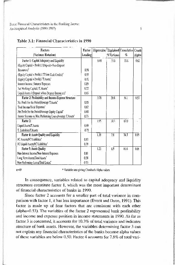
Table 3,1 shows that financial characteristics of commercial banks are grouped under five factors for the year 1990. In practice, variables explaining variance larger than variance of each variable are included in the model (Norusis, 1993), Thus, out of 18 principal components, only those with an eigenvalue greater than 1 are included in the model.

The first column in the table shows factors of the model and variables determining these factors. Factor loading defines to what extent variables affect factors and correlation coefficients between variables and factors. Hence, the most important variable determining factor 1 is the variable (Equity Capital+Profit)/ (Deposit+Non-Deposit Resources) which has the highest factor loading value. Eigenvalue column demonstrates to what degree factors account for total variance of 18 financial ratios. Thus, factor 1 explains 6.40 of the total variance. While factor 1 accounts for 35.6 % ([6.40/181*100) of total variance, factor 2 explains20.6 % of the rest. The first five factors included in the model account for81.6 percent of the variance. As the part of the factors explaining total variance decreases, they become less important in determining financial characteristics. Accordingly, factor 1, which has no relationship with the other factors accounting for the rest of the total variance, is the most crucial factor. “Cronbach Alpha” values in the table represent internal reliability of variables. As a result, six variables, which have the highest factor loading, determine factor 1. On the other hand, alpha reliability values of these six variables are below 0.50 (around 0.39). Although this outcome may indicate that six variables explain a financial characteristics, it also means that they randomly come together and there is an inconsistency among the variables. By leaving out each variable group consecutively, the reliability analysis is repeated to find out the variable causing low alpha value. For the factor 1, if we exclude “Interest Income/Interests Expenses)” variable, internal reliability among the other variables rises to an acceptable level (0.62). Hence, it is necessary to leave out this variable from the model. Variables with (*) sign denote variables producing acceptable alpha values.


Table 3.1: Financial Characteristics in 1990

Factors (Varimax Rotation}

FactorLoading

Eigenvalue Explained % Variance

Cumulative%

CroahAlpha

Factor I: Capital Adequacy and Liquidity(Equity Capita! + Profi!) / (Deposit +Non-Deposil Resources)'(Equity Capital + Profit) / (T.Non-Cash Credits)' {Equity Capital + Profit)/T. Assets' interest Income / Interest Expenses Ne! Working Capital / T. Assets*Liquid Assets / (Deposit +Non-Deposit Resources)*

0.960.950.920.890.720.65

6.40 35.6 35.6 0.62

Factor 2: Profitability and Income-Expense StructureNet Profit for the Period/Average TAssets*Total Income/Total Expenses*Net Profit for the Period/Average Equity Capital* interest Income on Non-Performing Loans/Average T.Assets*

0.950.820.800.73

3.70 20.6 56.1 0,53

Factor 3;Liquid Asseis/F. Assets T. Liabilides/LAssels

0.89-0.75

1.95 10.3 67.0

Factor 4: Assets Quality and LiquidityFC Assests/FC Liabilities*FC Liquid Assets/FC Liabilities’

0.930.79

1.39 7.8 111 0.85

Factor 5: Assets Quality Non-Interest income/Non-Interest Expenses Long Term Assets/Total Assets’ Non-Performing Loans/Total Loans*

0.810.580.53

1.23 6.9 81.6 0.68

n=49 * Variable sets giving Cronbach Alpha values

In consequence, variables related to capital adequacy and liquidity structures constitute factor 1, which was the most important determinant of financial characteristics of banks in 1990.

Since factor 2 accounts for a smaller part of total variance in comparison with factor 1, it has less importance (Everit and Dunn, 1991). This factor is made up of four factors that are consistent with each other (alpha=0.53). The variables of the factor 2 represented bank profitability and income and expense position in income statements in 1990. As far as factor 3 is concerned, it accounts for 10.3% of total variance and indicates structure of bank assets. However, the variables determining factor 3 can not explain any financial characteristics of the banks because alpha values of these variables are below 0.50. Factor 4 accounts for 7.8% of total vari

Osman Karamustafa

ance and is determined by two variables with alpha values above 0.50. These variables indicate the resources obtained from foreign currencies are invested as foreign currency deposited as liquid assets. Considering that alpha values of these variables are 0.85, we can argue that factor 4 explains a financial characteristics of the bank's. This factor can be named after the variables as “assets quality and liquidity”. Regarding factor 5, it explains about 7% of the total variance and is determined by three variables with factor loading above 0.50. Nonetheless, these variables have alpha values of 0.12. When reliability analysis is repeated by excluding “Non-Interest Income / Non-Interest Expenses” variable, alpha values rose to 0.68. As we define this factor in terms of the other two variables, it can be seen that this factor determines assets quality of the banks.

The table 3.2 illustrates financial characteristics for 1991. The most important factor explaining basic financial characteristics is determined by 7 variables and accounts for 44.1 percent of total variance. Reliability of the variables with each other is 0.58 but if we exclude “Interest Income/Interest Expenses” variable from the factor group, alpha value goes up to 0.65. Hence, it is necessary not to include this variable in the model. Upon a closer examination, it can be seen that variables showing the most important financial characteristics of the banks in 1991 were those financial ratios related to capital adequacy.


Table 3.2: Factor Analysis Results for 1991

Factors 1991 (Varimax Rotation)

FactorLoading

Eigenvaiue Explained % Variance

Cumulative%

CroahAlpha

Factor 1: Capital Adequacy (Equity Capital + Profit) / (Deposit+Non-Deposit Resources)*Interest Income / Interest Expenses (Equity Capital+Profit)/ (T. Assets+Non-casb Credits)* Liquid Assets / (Deposit* Non-Deposit Resources)* (Equity Capital + Profit) / T. Assets *Net Working Capital /T, Assets *Net Interest Income on Non-Performing Loans/Average T. Assets’

0.950.940.920.910.890.84

0.73

7.93 44.1 4.1 0.65

Factor 2; Profitability & Income-Expense StructureNet Profit for the Period / Average Equity Capital*Total Income / Total Expenses*Net Profit for the Period / Average T. Assets

0.910.730.69

3.36 18.7 62.8 0.65

Factor 3;Liquid Assets / T. Assets T. Loans/T. Assets FC Liquid Assets / FC Liabilities Non-Perfonning Loans /T . Loans

0.84-0.830.800.53

1.85 ■ 10.3 73.1

Factor 4:Non-Interest income / Non-Interest ExpensesNon-Performing Loans / T. LoansLong Term Assets / T. AssetsFactor 5: Equity Capital ProfitabilityNet Profit for the Period / Average Paid-up Capital

0.81'0.640.62

1.22

1.06

6.8

5.9

79.9

85.8


Factor 2 accounts for 18.7 percent of total variance and factor loading consists of 3 variables, which have alpha values of 0.60. If “Net Profit for the Period / Average Total Assets” is left out, alpha increases to 0.65. Thus, if we define this factor on the basis of “Net Profit for the Period/Average Equity Capital and “Total Income/Total Expenses variables, factor 2 represents profitability and income-expense structure of the banks.

Since alpha values of variables constituting factor 3 and factor 4 are below 0.50, we can suggest that the variables are grouped within these factors randomly. Therefore, factor 3 and factor 4 do not demonstrate any

Osman Karamustafa

financial dimension of the banks. Regarding factor 5 in the table 3.2, it only accounts for 5.9% of the total variance.

The analysis reveals 6 main factors for 1992 (see table 3.3). Nevertheless, factor 2 has an alpha value of 0.24, which means that it does not explain any financial characteristics of the? banks. Hence, the remaining five factors indicate basic financial characteristics.


Factors {Varimax Rotation)

FactorLoading

Eigenvalue Explained%Varianct

Cumulative%

CroahAlpha

Factor 1: Capital Adequacy(Equity Capita! + Profit) / T. Assets*(Equity Capital+Profit)/(T. Assets +Non-Cash Credits)* Net Working Capital / T. Assets’(Equity Capital+Profit)/(Deposit+Non-Deposit Resources)

0.970.920.890.77

4.98 27.7 27.7 0.94

Factor 2:Total Income / Total ExpensesNet interest Income on Non-Performing loans/Average T. AssetsFC Assets / FC LiabilitiesLong Term Assets / T. AssetsInterest Income / Interest ExpenseNet Profit for the Period / Average T. Assets

0.77

0.67-0.60-0.600.570.55

3.20 17.8 45.5

Factor 3: Liquidity StructureFC Liquid Assets/ FC Liabilities T.Loans IT. Assets Liquid Assets/T. Assets*

0.91-0.810.78

2.37 13.2 58.7 0.70

Factor 4: Profitability of Equity Capital Net Profit for the Period / Average Equity Capital 0.84

1.50 8.4 67.1

Factor 5: Liquidity StructureLiquid Assets / (Dcposilf Non-Deposit Resources) 0.91

1.15 6.4 73.5

Factor 6: ProfitabilityNet Profit for the Period / Average Paid-up Capital 0.86

1.10 6.2 79.6

n—54 * Variable sets giving Cronbach Alpha values

Factor 1 is the most important principal component explaining 27.7% of total variance. Alpha values determining four variables of this factor are around 0.62. If “(Equity Capital+Profit)/(Deposits+Non-Deposit Resources)” variable is excluded, alpha values go up to 0.94. Taking all the remaining variables into consideration, this factor determines capital adequacy of the banks.


Factor 3 accounts for 13.2% of the total variance. If we do not include “Total Credits / Total Actives” variable in the model, alpha rises to 0.70. Hence, factor 3 is determined by “Liquid Assets/ Total Assets” and “FC Liquid Assets / FC Liabilities” and represents liquidity structure of the banks.

The last 3 factors for 1992 are affected by a variable. Thus, factor 4, factor 5 and factor 6 account for 8.4%, 6.4% and 6.2% of total variance and denote equity capital profitability, liquidity structure and bank profitability, respectively. We found four factors that explain 81 % of total variance for 1993 (see, table 3.4). Yet, since variables constituting factor 4 have low alpha values, they do not have any explanatory power.


Factors (Varimax Rotation)

FactorLoading

Eigenvalue Explained%Variance

Cumulative%

CroahAlpha

Factor 1: Capital - Assets Quality (Equity Capital + Profit) / (T.Assets+Non-Cash Credits)* FC Assets / FC Liabilities'(Equity Capital + Profit) / TAssets*(Equity Capita 1+Pr ofit)/(Depos it+Non-Deposit Resources) FC Liquid Assets / FC Liabilities Interest Income / Interest Expenses Long Term Assets / T, Assets*

0.920.910.850.840.830,820.77

6.11 34.0 34.0 0.79

Factor 2; Profitability and Income- Expense Structure

Net Profit for the Period / Average Equity Capital* Net Profit for the Period / Avarage Paid-up Capital* Non-Interest Income / Non-interest Expense*Total Income / Total Expenses’Non-Performing Loans / T. Loans

0.810.80-0.750.68-0.60

5.07 28.2 62.2 0.85

Factor 3: Profitability and Income- Expense Structure

Net Working Capital / T. Assets Net Profit for the Period / Average T. Assets* Net interest Income on Non-Performing Loans/ Average T.Assets*

0.840.83

0.78

2.02 11.2 73.4 0.83

Factor 4:Total Loans / Total AssetsLiquid Assets / Total AssetsLiquid Assets / (Deposit+Non-Deposit Resources)

-0.830.810.57

1.32 7.4 80.8

n-55 * Variable sets giving Cronbach Alpha values

10 Osman Karamustafa

Factor 1 reveals the most important financial characteristics of banks as it accounts for a significant part of the total variance. Alpha values of the related variables are about 0.55. If “Interest Income / Interest Expenses” variable is left out, it increases to 0.79. Hence, variables related to capital adequacy and assets quality constitute the most important factor that explains basic financial characteristics of the banks in 1993. Factor 2 accounts for 28.2% of total variance. If “Non-Performing Loans/ Total Loans” variable is excluded, alpha value rises to 0.85. Factor 2 based on four variables in the above table denotes profitability of the banks. With regard to factor 3, if “Net Working Capital / Total Assets” variable is not included, alpha value goes up to 0.83. This factor accounts for 11.2 % percent of total variance and represents profitability of the banks.

For 1994, factor 3 and factor 5 are excluded from the analysis as alpha values of these factors are below 0.50. The remaining three factors determine financial characteristics of the banks (see table 3.5). Factor 1 describing profitability of banks and capital adequacy explains 40.7% of the total variance and is therefore the most important principle component.

Factor 2 accounts for 16.2% of the total variance. If we exclude “Liquid Assets / (Deposit+Non-Deposit Resources)” variable, alpha value increases to 0.53. As a result, this factor denotes profitability and income- expense structures of the banks. In addition, factor 4 defines liquidity structure of the banks and consists of (“Liquid Assets / Total Assets” and “FC Liquid Assets / FC Liabilities) variables with an alpha value of 0.76.


Table 3.5 : Factor Analysis Results for 1994Factors

(Varimax Rotation)Factor

LoadingEigenvalue Explained

^VarianceCumulative

%CroahAlpha

Factor 1: Profitability and Capital Adequacy Net Profit for the Period / Average Total Assets' Total Income / Total Expenses'Net Interest Income on Non-Performing Loans/ Average TAssets4Net Profit for the Period / Avarage Paid-up Capital Net Working Capital / T. Assets *(Equity Capital + Profit) / T. Assets*

0.920.83

0.830.800.670.61

7.32 40.7 40.7 0.72

Factor 2: Profitability&Income-Expense Structure(Equity Capital+Profit)/(Deposit+Non-Deposit Resources)* (Equity Capital + Profit)/(T. Assets+Non-Cash Credits)* Interest Income / interest Expenses*(Equity Capitai + Profit) / TAssets*Liquid Assets / (Deposit-i- Non-Deposit Resources)

0.810.780.730.690.53

2.91 16.2 56.9 0.53

Factor 3:Net Profit for the Period / Average Equity Capital Non-Performing Loans/T. Loans*Long Term Assets / T. Assets1

0.950.920.70

1.81 10.1 67.0

Factor 4: LiquidityLiquid Assets / Total Assets* Total Loans / Total Assets FC Liquid Assets/ FC Liabilities*

0.87-0.780.69

1.54 8.6 75.6 0.76

Factor 5:Non-Interest Income / Non-Interest Expense FC Assets/FC Liabilities (Equity Capital + Profit) / TAssets

0.900.83

1.44 8.0 83.6

n=55 * Variable -sets g iv in g Cronbach Alpha values

The tablé 3.6 illustrates that three factors determine financial characteristics of the banks for 1995. Alpha values of variables with (*) are around 0.93 and constitute factor 1. The high alpha value means that these variables are of considerable significance in defining this factor, which represents profitability and capital adequacy of the banks


12 Osman Karamustafa


FactorLoading

Eigenvalue Explained % Variance

Cumulative%

CroahAlpha

Factor 1: Profitability and Capita! Adequacy Net Profit for the Period / Average Total Assets1 (Equity Capital + Profit) / (T.Assets+Non-Cash Credits)* (Equity Capital + Profit) / T,Assets*Net Profit for the Period / Avarage Paid-up Capital Net Working Capital / T. Assets*Net Interest Income on Non-Performing Loans/Average T. Assets*

0.850.840,760.760.75

0.68

7.12 39.6 39.6 0.93

Factor 2: Income-Expense Structure,Capital Adequacy and Liquidity

Interest Income / Interest Expense*(Equity Capital+Profit)/(Deposit+Non-Deposk Resources)* Liquid Assets / (Deposit+Non-Deposit Resources)’Total Income / Total Expenses*

0.930.860.700.63

2.93 16.3 55.9 0.53

Factor 3: Liquidity and Assets Quality Total Loans /Total Assets Liquid Assets / Total Assets*FC Liquid Assets / FC Liabilities* Non-Performing Loans /T. Loans’

-0.820.800.740.73

2.48 13.8 69.8 0.68

Factor 4:FC Assets / FC Liabilities Non-Interest Income / Non-Interest Expenses

0.880.75

1.25 7.0 76.7

FactorS:Net Profit for the Period / Average Equity Capital Long Term Assets j Total Assets

0.75-0.75

1.00 5.6 82.3


Internal reliability of variables constituting factor 2 is 0.53. This factor explains 16.3% of total variance and defines capital adequacy and liquidity structure. “Liquid Assets/Total Liabilities” and “Non-Performing Loans / Total Loans” variables determine factor 3. It accounts for 13.8% of total variance and represents liquidity and assets structure of the banks. The first three factors in the table 3.7 represent basic financial characteristics of the banks in 1996. Factor 1 accounts for 33.6% of the total variance and is made up of capital adequacy and assets quality variables, which have an alpha value of 0.71.


Table 3.7: Factor Analysis Results for 1996Factors

(Varimax Rotation)Factor

LoadingEigenvalue Explained

%VarianaCumulative

%CroahAlpha

Factor 1: Capital Adequacy and Assets Quality (Equity Capital+Profit)/(Deposit+Non-Deposit Resources) (Equity Capital + Profit) / (T.Assets+Non-Cash Credits)* (Equity Capital + Profit) / T.Asscts'Interest Income / Interest Expenses Long Terra Assets / Total Assets*

0.940.900.890.860.73

6.04 33.6 33.6 0.71

Factor 2: Profitability&Income-Expense StructureNet Profit for the Period / Average Total Assets’Total Income / Total Expenses*Net Profit for the Period / Average Equity Capital*Net Working Capital / T. Assets

0.900.860.750.64

4.03 22.4 56.0 0.61

Factor 3: LiquidityLiquid Assets / Total Assets*Total Loans /Totai Assets FC Liquid Assets /F C Liabilities’Liquid Assets / (Deposit+Non-Deposit Resources)*

0.91-0.840.740.67

2.50 13.9 69.9 0.72

Factor 4:Non-Interest Income / Non-Interest Expenses FC Assets/FC Liabilities Net Interest Income on Non-Performing Loans/ Average T.Assets

0.930.79

-0.66

1.38 7.7 77.5


Factor 2 is defined by four variables, which have factor loading above0.50. These variables explain a principal component provided that “Net Working Capital / Total Assets” variable is excluded from the model. Reliability coefficient of the other three variables is 0.61. Hence, factor 2 defines profitability and income-expense structure. Factor 3 represents Liquidity structure of the banks and explains 13.9 % of the total variance. It is determined by three variables with an alpha value of 0.72 (see, table 3.7).

Table 3.8 presents financial characteristics for 1997. Five principal independent components are determined on the basis of factor analysis. As a result of reliability test, the first three factors were found to determine basic financial characteristics of the banks in 1997. Alpha value of four variables constituting factor 1 is 0.67. This further demonstrates that these variables are consistent with each other. Compared to the other four

Osman Karamustafa.;

factors, this principal component accounts for the largest part of the total variance (33.5%) and is the most important financial characteristics of the banks. Considering factor loading, this factor can be called as “capital adequacy and assets quality” of banks.



FactorLoading

Eigenvalue Explained%Variance

Cumulative%

CroahAlpha

Factor 1: Capital Adequacy and Assets Quality (Equity Capital+Profit)/(Deposit4-Non-Deposit Resources)’ (Equity Capital+Profit)/(T,Assets+Non-Cash Credits)* (Equity Capital + Profit/T,Assets’Long Term Assets / Total Assets’

0.930.920.910.73

6.03 33.5 33.5 0.67

Factor 2: Profitability, Capital Adequacy and Income-Expense Structure

Net Profit for the Period / Average Total Assets*Net Working Capital / T. Assets’Net Interest Income on Non-Performing Loans/ Average TAssets*Total Income / Total Expenses

0.860.82

0.640.60

3.66 20.4 53.9 0.84

Factor 3: LiquidityLiquid Assets / Total Assets*Total Loans/Total Assets FC Liquid Assets / FC Liabilities’

0.91-0.880.70

2.27 12.6 66.6 0.68

Factor 4:FC Assets / FC LiabilitiesNon-Interest Income/ Non-Interest ExpensesNet Profit for the Period / Avarage Paid-up Capital

0.920.91-0.61

1.92 10.7 77.2

Factor 5:Non-Performing Loans / Total Loans \ Net Profit for the Period / Average Equity Capital

-0.90 : o.73 :

1.35 ; 7.5 84.8 ;

n_55 * Variable sets giving Cronbach Alpha values

Since alpha value of the first three variables that constitute factor 2 is 0.84, these variables are important in defining this factor. Factor 2 accounts for 20.4 % of the total variance and defines profitability, capital adequacy and income-expense structure of the banks. Two variables (“Liquid Assets/Total Assets” and “FC Liquid Assets/FC Liabilities”) determine factor 3, which explains 10.7% of the total variance and describes liquidity structure of banks.


IV. Stability of Financial CharacteristicsWhether the ranking of the variables in terms of years are meaningful at the same significance level determines stability of financial characteristics of banks in a certain period. In this study, we determine whether the variables constituting the factors are in the same rank through the use of “Sperman Correlations”.

The table 4.1 shows if factor 1, which is the most significant financial characteristic, has a stable structure in the period of 1990-97. The variables determining factor 1 are in the same rank at a significance level of 0.05 or 0.01 except 1994. This reveals that the variables have a stable structure in the period under consideration except 1994. It can be argued that crisis in 1994 had negative effects on the stability of the financial characteristics of banks.

Table 4.1: Factor 1 Sperman Correlations

Factor 11991 ,8287**1992 ,7255** ,7007**1993 ,7957** ,5996** ,6429**1994 0,2755 ,5005* 0,4283 0,06091995 ,4716* ,6429** ,5542* 0,2074 ,8947**1996 ,9608** ,7792** ,7379** ,8473** 0,1827 0,37051997 ,8824** ,6842** ,6615** ,7317** 0,0361 0,2755 ,9422**

1990 1991 1992 1993 1994 1995 1996

* -Significance level,05 ** Significance level -,01 (2-tailed)

Factor 2 is composed of variables related to profitability and income- expense structures of banks. Variables associated with capital adequacy and liquidity structure have a considerable part in determining these factors in 1995 and 1997. The table 4.2 illustrates in which periods variables constituting factor 2 are stable at a statistically significant level.

Osman Karamustafa


Factor 21991 ,7709**1993 ,6140** ,6863**1994 -0,129 -0,16 -0,1331 ,y1995 0,257 0,2074 0,1558 ,8060**1996 ,7957** ,8885** ,6388** 0,063 0,44481997 ,7461** ,7069** ,5418* 0,2054 0,4365 ,8535**

1990 1991 1993 1994 1995 1996*- Significance level ,05 **- Significance level,01 (2-tailed)

In consequence, factors in 1994 and 1995 did not exhibit stability with the other factor variables. With the exception of these periods, all the factors are stable at a significance level of 0.05 or 0.01.

The table 4.3 presents whether variables of factor 3 have a stable structure in the periods under examination. The variables of this factor were stable at a signficance level of 0.05 in 1992, 1995 and 1996 and they were stable with each other at a significance level of 0.01 in 1995, 1996 and 1997.


Factor 31993 -0,3541995 ,5088* -0,15581996 ,4985* -0,1042 ,8906**1997 0,4303 0,1476 ,7461** ,8101**

1992 1993 1995 1996* - Significance level ,05 **- Significance level ,01 (2-tailed)

As can be seen in the table 4.4, factor 4 does not have a stable structure in the periods under consideration.


Factor <■1992 -0,34371994 0,3746 -0,1187

1990 1992 1994

* - Significance level i ,05 **- Significance level, 01 (2-tailed)


Factor 5 only exhibits stability between 1990 and 1992 (see, table4.5)


Factor 51991 -0,12691992 -,7049** 0,1806

1990 1991 1992* - Significance level ,05 **- Significance level, 01 (2-tailed)

V. Concluding RemarksThis paper offers an analysis of how financial characteristics of commercial banks operating in Turkish financial system developed between 1990- 1997. The results of the study can be summarised as follows:

Variables describing the most important financial characteristics of the banks are generally those connected with capital adequacy of the banks. In addition, variables related to profitability determined factor 1 in 1994 and 1995. Considering that the system was in crisis in both years, it can be pointed out that periods in which capital adequacy is not the most important financial characteristic indicate a crisis in the banking system. Capital adequacy became the most crucial characteristics of the banks together with variables representing assets quality of the banks in 1996 and 1997.

The first three factors are the most significant factors determining financial characteristics because they account for a greater part of total variance. Variables related to capital adequacy exhibit stability year by year. This structure loses its stability relatively as the significance of the factors decreases. During the 1994 crisis, stable structures among the variables determining financial characteristics collapsed.

Although equity capital comprises a small part within total liabilities, its function as creating trust between depositors, other organizations and banks, reducing losses and being a fund resource for banks demonstrates the indispensability of capital adequacy for banks. Variables revealing capital structures of banks are more important than the other financial variables for interest groups in their decision-making process.

Osman Karamustafa

ReferencesA L T M A N , E d w a rd I ., “ F in a n c ia l R a tio s , D is c r im in a n t A n a ly s is o f th e P r e d ic t io n o f

C o rp o ra te B a n k ru p tc y ” , J o u rn a l o f F in a n c e , 2 3 , p p 5 8 9 -6 0 9 , S e p te m b e r 1 9 6 8 .A K T A Ş , R a m a z a n , “ E n d ü s tr i İ ş le tm e le r i iç in M a l i B a ş a r ıs ız l ık T a h m in i (Ç o k

B o y u tlu M o d e l U y g u la m a s ı) ” , T ü r k iy e İş B a n k a s ı K ü l tü r Y a y ın la r ı N o :3 2 3 , A n k a ra , 1 9 9 3 . .5

B A N K A L A R IM IZ 19 9 7 , T ü rk iy e B a n k a la r B ir l iğ i , M a y ıs 1998 .B E A V E R , W ill ia m H ., “ F in a n c ia l R a tio s a s P re d ic to r s o f F a i lu r e ” E m p ir ic a l R e s e a rc h

in A c c o u n t in g ” S e le c te d S tu d ie s , V o l.4 , p p 7 1 -1 1 1 , 1966 .D İ N C E , R .R ., C . F O R T S O N , “ T h e U s e o f D i s c i r im in a n t A n a ly s is to P r e d ic t th e

C a p i ta l A d e q u a c y o f C o m m e rc ia l B a n k s ” , J o u rn a l o f B a n k R e s e a rc h , p p 5 4 - 6 2 , S p r in g , 1 9 7 2 .

E D M I S T E R , R o b e r t O ., “ A n E m p ir ic a l T e s t o f F in a n c ia l R a t io A n a ly s is fo r S m a ll B u s in e s s F a i lu re P re d ic t io n ” , J o u rn a l o f F in a n c ia l a n d Q u a n ti ta t iv e A n a ly s i s ” , p p 1 9 7 7 -9 3 , M a rc h 1972 .

E V E R 1 T T , B .S . a n d D U N N , G ., A p p l ie d M u l t iv a r ia te D a ta A n a ly s is , L o n d o n : E d w a r d A rn o ld , 1991 .

G O M B O L A , M ic h a e l J ., J. E d w a rd K E T Z , “ F in a n c ia l R a t io P a t te rn s in R e ta i l a n d M a n u f a c tu r in g O r g a n iz a t io n s ” ,F in a n c ia l M a n a g e m e n t , p p 4 5 -5 6 , S u m m e r , 1983 .

G Ö K T A N , E rk u t , “ M u h a s e b e O ra n la r ı Y a rd ım ıy la v e D is k r im in a n t A naliz ; T e k n iğ in i K u l la n a ra k E n d ü s tr i İ ş le tm e le r in in M a l i B a ş a r ıs ız l ığ ın ın T a h m in i Ü z e r in d e A m p ir ik B ir A r a ş t ı r m a ” , B a s ı lm a m ış D o ç e n t l ik T e z i, 1 9 8 1 .

H A IR , Jr. J o s e p h , R o lp h e E . A N D E R S O N , R o n a ld L . T A T H A M , W il l ia m C . B L A C K , “ M u ltiv a r ia te D a ta A n a ly s is W ith R e a d in g s ” , 5 .B a s k ı, P re n t ic e - H a ll , ın c , U S A , 1 9 9 8 .

H O R R IG A N , J a m e s O ., “ A S h o r t H is to ry o f F in a n n c İa l R a tio A n a ly s i s ” T h e A c c o u n t in g R e v ie w , 4 3 , p p 2 8 4 -2 9 4 . , 1 9 6 8 .

J A C K E N D O F F , N a th a n ia l , “ A S tu d y o f P u b li s h e d I n d u s t r y F in a n c ia l a n d O p e ra t in g R a t io s ” , S m a ll B u s in e s s M a n a g e m e n t R e s e a rc h R e p o r t , U S A , T e m p le U n i, , 196 2 .

L A U R E N T , C .R ., “ I m p ro v in g T h e E f f ic ie n c y a n d E f f e c t iv e n e s s o f F in a n c ia a l R a tio A n a ly s i s ” , J o u rn a l o f B u s in e s s F in a n c e & A c c o u n t in g , 6 ,3 , p p 4 0 1 -1 3 , 1 9 7 9 .

M A R T IK A IN E N , T e p p o , “ S to c k R e tu rn s a n d C la s s if ic a t io n P a t te rn o f F i r m - S p e c if ic F in a n c ia l V a ria b le s : E m p ir ic a l E v id e n c e W ith F in n is h D a ta ” , J o u rn a l o f B u s in e s s F in a n c e & A c c o u n t in g , 2 0 (4 ) , p p 5 3 7 - 5 5 7 , J u n e 1993 .

M A R T IN , A lv in , “ A n E m p ir ic a l T e s t o f th e R e le v a n c e o f A c c o u n t in g In f o rm a t io n fo r I n v e s tm e n t D e c i s io n s ” , J o u r n a l o f A c c o u n t i n g R e s e a r c h , p p 1 -3 1 , S u p p le m e n t , 197 1 .

M E Y E R , P a u l A ., H o w a rd W . P IF E R , “ P re d ic t io n o f B a n k F a i lu r e s ” , J o u rn a l o f F in a n c e , p p 8 5 3 -6 3 , S e p te m b e r , 1 9 7 0 .

N O R U S IS , M a r i ja J . , “ S P S S fo r W in d o w s P r o fe s s io n a l S ta t is t ic s - R e le a s e 6 .0 ” , S P S S In c , C h ic a g o , U S A , 1 9 9 3 .

P E T T W A Y , R .H ., J.F . S IN K E Y , “ E s ta b l i s h in g O n - S i te B a n k E x a m in a t io n P r io r i ty :A n E a r ly W a rn in g S y s te m U s in g A c c o u n t in g a n d M a r k e t I n f o rm a t io n ” , J o u rn a l o f F in a n c e , p p 1 3 7 -5 0 , M a r c h 1980 .

P IN C H E S , G e o rg e E „ K e n t A . M IN G O , J .K e n t, C A R U T H E R S , “ T h e S ta b i l i ty o f P a t te rn s in In d u s t r ia l O r g a n iz a t io n s ” , T h e J o u rn a l o f F in a n c e , Vo 1:28, N o :3 , p p 3 8 9 -9 6 , 1973 .

Basic Financial Characleristics in the Banking Seclor:An Empirical Analysis (1990-1997) 19

P IN C H E S , G e o rg e E ., K e n t A . M IN G O , “ A M u lt iv a r ia te A n a ly s is o f I n d u s t r ia l B o n d R a t in g s ” , J o u rn a l o f F in a n c e , 2 8 , p p 1 -1 8 , M a rc h 1973 .

S IN K E Y , J .F ., “ A M u l t iv a r ia te S ta t is t ic a l A n a ly s is o f th e C h a ra c te r is t ic s o f P ro b le m B a n k s ” , J o u r n a l o f F in a n c e , p p 2 1 -3 6 , M a rc h , 1975 .

O ’C O N N O R , M e lv in C . “ O n th e U s e fu ln e s s o f F in a n c ia l R a t io s to In v e s to r s in C o m m o n S to c k ” , T h e A c c o u n t in g R e v ie w , p p 3 3 9 -3 5 2 , A p r i l 197 3 .

The ISE Review Volume: 3 No: 9 January/February/March 1999 ISSN 1301-1642 © ISE 1997

LEADING INDICATORS APPROACH FOR BUSINESS CYCLE FORECASTING AND

A STUDY ON DEVELOPING A LEADING ECONOMIC INDICATORS INDEX FOR THE

TURKISH ECONOMY

Ali MÜRÜTOĞLU*

AbstractB u s in e s s c y c le s , o n e o f th e m a in c h a ra c te r is t ic s o f d e v e lo p e d c o u n t r i e s ’ e c o n o m ie s , h a v e b e g u n to p la y a n im p o r ta n t r o le fo r th e T u rk is h E c o n o m y . E s p e c ia l ly a f te r th e 1 9 9 4 c r is is (w h ic h w a s o n e o f th e m o s t s e v e re o n e s in c e th e f o u n d a tio n o f T u rk is h R e p u b l ic ) a n d th e c u r r e n t s lo w -d o w n o f th e e c o n o m y ( m a in ly b e c a u s e o f th e g lo b a l c r is is w h ic h s te m m e d f ro m th e s o u th -e a s t A s ia n c o u n tr ie s a n d R u s s ia ) , i t h a s b e c o m e v i ta l to fo r e s e e th e fu tu re o f th e e c o n o m y (i .e . w h ic h p h a s e th e e c o n o m y w il l b e in th e b u s in e s s c y c le in th e fu tu re ) fo r th e d e c is io n m a k e r s b o th in p u b l ic a n d p r iv a te s e c to rs . T h u s , i t c a n b e p o s s ib le to ta k e c o n t r a r y a c t io n s to r e d u c e th e h a r m f u l e f fe c ts o f r e c e s s io n s .

O n e m e th o d o f s h o r t - te r m fo r e c a s t in g o f e c o n o m ic c o n d i t io n is th e L e a d in g E c o n o m ic I n d ic a to r s A p p r o a c h w h ic h is th e s u b je c t o f th is s tu d y . In th is s tu d y , a f te r e x p la in in g b u s in e s s c y c le s a n d L e a d in g E c o n o m ic In d ic a to rs A p p r o a c h to fo r e c a s t th e b u s in e s s c y c le s , I a n a ly z e n e a r ly 5 0 e c o n o m ic t im e s e r ie s to f in d a L e a d in g E c o n o m ic In d ic a to r s In d e x fo r th e T u rk is h e c o n o m y .T h e r e s u l t in g in d e x is c o m p r is e d o f n in e e c o n o m ic s e r ie s w h ic h a r e s ta n d a r d iz e d a n d c o m p o s e d w i th e q u a l w e ig h t to fo r m “ T h e L e a d in g In d ic a to rs In d e x f o r th e T u rk is h E c o n o m y ” . T h e s e r ie s a re a s fo llo w s ; T o ta l I m p o r t o f I n v e s tm e n t G o o d s , T o ta l I m p o r t o f In te r m e d ia te G o o d s , C u rre n c y , M 2 , R e s e r v e M o n e y , D e p o s i t M o n e y B a n k s ’ C r e d i t s , N e t C r e d i t V o lu m e , C o n s o l id a te d B u d g e t M o n t h ly E x p e n d i tu r e s , T o ta l C a p i t a l o f N e w ly E s ta b l is h e d F irm s .

L introductionGenerally, two kinds of movements can be observed in the economies of the countries with free market economic system. These movements are

* Floor Specialist in the Bonds and Bills Department at the Istanbul Stock Exchange Address: IMKB Tahvil ve Bono Piyasası 80860 Istinye, Istanbul, Phone: 0-212-2982578, e-mail: amurut@lycoserriailcom)The view and opinions expressed here are those of the author and do not reflect those of îhe ISE.

22 Ali Miiriitoglu

the long-run growth (or decline) and short-run fluctuations. Long-run growth (or decline) can be defined as the trend observed in the general economic indicators (such as GNP, employment, industrial production, investment etc) in the long run. On the other hand, short-term fluctuations are the changes of the economic variables (0NP, industrial production, employment, interest rates etc) around this long-run trend. The fluctuations show a cyclical characteristic and are called business cycles.

In recent years, business cycles have become important for Turkey in parallel with the efforts for transforming its economy from planned to free-market economy. As a result, forecasting business cycles has become a necessity for the Turkish economy.

Various kinds of methods have been used in the short-run forecasting of economic activity. These methods vary from the qualitative types, based mainly on the experience and knowledge of the forecaster, to the quantitative methods (e.g., econometric models which are very complicated and based on the cause and effect relationship in the economy). Leading Economic Indicators Approach, one of the types of these methods, is the topic of this paper.

In this study, after providing brief information about business cycles, leading indicators are considered in detail. After examining the leading indicators approach in the world and Turkey, a “Leading Economic Index for the Turkish Economy” is developed in the last section.

II. Business CyclesSeveral definitions of business cycles have been proposed in the literature so far. Among these, the definition proposed by Arthur F. Burns and Mitchell C. Wesley (1946) is the most comprehensive and widely accepted. According to this definition, business cycles are types of fluctuations found in the aggregate economic activity of nations that organize their work mainly in the business enterprise. A cycle consists of expansions occurring at about the same time in many economic activities, followed by similarly general recessions, contractions and revivals which merge into the expansion phase of the next cycle. This sequence of changes is recurrent but not periodic; the time span of business cycles vary from more than one year to ten or twelve years. They are not divisible into shorter cycle of , similar character with amplitudes approximately their own.

On the other hand, some authors claim business cycles of 50-60

Leading Indicators Approach for Business Cylcle Forecasting and a Study onDeveloping a Leading Economic Indicators Index for the Turkish Economy 23

years in length. Especially Kontradief and Schumpeter (1939) argue that business cycles cover 50-60 years period and do not only reflect economic changes but also social changes. However, this definition does not have many advocates.

Business cycles can be divided into two periods. The period that starts from the beginning trough to the end of the peak of the cycle is called the expansion period, from the peak to the ending trough is called the contraction period. Expansion period is further divided into two phases. From the beginning trough to the half of the expansion period is called the recovery phase, from the end of the recovery phase to the peak is called the prosperity phase. Also the contraction period is divided into two phases. The phase that starts from the peak and ends at the middle of the contraction period is called the crisis phase. In this phase, the economic activity declines sharply. The phase from the middle of the contraction period to the next trough is called the recession phase. If the recession phase is long and deep it is called the depression.

III. Leading Indicators ApproachLeading indicators approach assume that economic fluctuations are inevitable. In a certain business cycle, all economic time series do not

Ali Miiriitoglu

move with the general economic condition. Some of them move before, some of them move at the same time while some others follow the general economic condition with a lag. Economic series which move before the general economic condition are called leading series, series that move with the general economic condition are called coinciding series and series that follow the general economic condition with a lag are called the lagging series. Leading indicators approach is based on determining the leading series and using them to forecast the condition of the economy in the near future.

Most of the leading series reflect the future plans about economic activities, decisions about the future and contracts that are related to the future. Economic series like new orders for goods and services, new constructions, activities in the intermediate goods industry, prices of raw materials and intermediate goods, etc. have the potential to show the direction of the future economic activity.

Although the leading indicators approach is an easy and practical way for forecasting economy’s future, it has some drawbacks; firstly, there are limited numbers of economic series that reflect the economic condition regularly. Even the best leading indicator provides forecast correctly at 80-90 per cent of the time. Secondly, the lead time of leading indicators is not stable, it changes with time. Lastly, even if we suppose that the leading indicators forecast the economic condition correctly, both with respect to time and direction, they cannot show the magnitude of the change in economic activity.

IV. Leading Indicators Approach in USA and Europe

A. Leading Indicators Approach in USAIn USA, currently 112 economic indicators are monitored continuously. They are updated when necessary. From these indicators, 61 of them are classified as leading, 24 of them are classified as coinciding and 19 of them are classified as lagging indicators. Remaining 8 indicators can not be classified. These indicators represent 7 different sectors of the economy. These sectors are:

1. Labor and Unemployment,2. Production and Income,3. Consumption, Trade and Sales,4. Fixed Income Investments,

5. Stocks,6. Prices, Costs and Profit7. Money and Credit.

U.S. Department of Commerce, Bureau of Economic Analysis has done studies related to these kind of economic indicators. Findings are published in the monthly periodical Business Conditions Digest. Leading Indicator Index for the US economy is also published in this periodical. There are 11 leading, 4 coinciding and 7 lagging economic indicators stated in Business Conditions Digest. Components of Leading Economic Index of the US economy are follows:1. Average workweek, production workers, manufacturing2. Layoff rate, manufacturing3. Net orders for consumer goods and materials, 1972 dollars4. New building permits, private housing5. Vendor performance, percent of companies receiving slower delivery6. Performance in the sales and deliveries7. Changes in sales prices of important materials8. Consumer expectations index9. Money supply, M2, 1972 dollars10. Contracts and orders for plant and equipment, 1972 dollars11. Stock prices, 500 common stock

Currently in USA, there are some studies for dividing leading indicators into short leading and long leading indicators and changing some of the economic series. The main objective of these studies is to form a Leading Index that reflects the services sector and international economic developments.

B. Leading Indicators for OECD Countries:OECD has been carrying out various studies about leading indicators in the member country’s economy. The OECD indicator system use of Index of Total Industrial Production as the reference series. OECD has been monitoring approximately 190 economic series from 8 main sectors of the economies’ of member countries. Some of these series cannot be monitored for all member countries. The different subject areas from which the leading indicator series are chosen are set out in Table 1.

Leading Indicators Approach for Business Cyicle Forecasting and a Study onpeveloping a Leading Economic Indicators Index for the Turkish Economy 25

Ali Mürütoglu

Table 1: Leading Indicators Used in OECD System

COUNTRIES

I. PRODUCTION, STOCKS AND ORDERS1. Industrial Productions in Specific Branches2. Oalers3. Stocks- Materials- Finished Goods- Imported Products

4. Ratios, e.g. inventory/shipment

I 2 3 4 5 6 7 8 y ¡0 ¡1 12 13 14 15 16 17 18 Î9 20 21 22 23

11

1

1

1

1) 1

1

121

21

1 54

24I1

II. CONSTRUCTION, SALES AND TRADES1. Constructions Approvals2. Construction Starts3. Sales or Registrations of Motor Vehicles4. Retail sales

11

1 I 11111

1

1

1 1 1

1

11

11

3655

HI. LABOUR FORCE1. Ratio, New Employment/Employment2. Layoffs/Initial claims, Unemployment Insurance3. Vacancies4. Hours Worked 1

1

1

1I

1

12 1 2

IV. PRICES, COSTS AND PROFITS1. Wages and Salaries Per Unil of Output2. Price Indices3. Profits

11 1

i2 1 I

1

2

362

V. MONETARY AND FINANCIAL1. Forcing Exchange Holdings2. Deposits3. Credit4. Ratios, e.g. Loans/Deposits5. Money Supply6. Interest Rates7. Slock Prices8. Company Formation

1

1

1

!111

11!11

1

1

1 11I

11

2

1 131

111

I

I 111

11

1

13

1

111

111

1

11

1

2241171412I

VI. FOREIGN TRADE1. Export Aggregates2. Export Components3. Trade Bilance4. Terms of Trade

11 1 1

2

1 1 1 1

1

1

12 16

V II. BUSINESS SURVEYS1. General Situation2. Production3. Orders inflow/New Orders4. Ordersbook/Sales5. Stock of Raw Materials .6. Stock of Finished Goods7. Capacity Utilization8. Bottlenecks9. Employment10. Prices

11

!

1

1

1II

1

1

1

11

i

I

1

121

1

11

1

I

11

1

I11 1

1

1

1

1

I

111

1

I11 1

11

1

2

21

1111

1i

1

1

111

6151!113102231

V III. ECONOMIC ACTIVITY IN FOREIGN COUNTRIES 1 5 2 1 9INDICATORS 12 9 11 8 f) 7 9 1Ü u 9 2 9 9 7 11 it 6 7 12 7 10 4 189

Source: Nilsson, Ronny, “Leading Indicators for OECD, Centra! and Eastern European Countries” in is the Economic Cycle Still Alive; Theory, Evidence and Policy edited by Mario Baldassari and Paulo Annunziato, St. Martin Press Inc. New York, 1994.

COUNTRIES1. Canada 7. Denmark 13. Ireland 19. Sweden2. USA 8. Finland i4. Italy 20. Switzerland3. Japan 9. France 15. Netherlands 21.UK4. Australia 10. Germany 16. Norway 22. Yugoslavia5. Austria 11. Luxembourg 17. Portugal 23. All Countries6. Belgium 12. Greece 18. Spain

Leading Indicators Approach for Business Cylcle Forecasting and a Study onDeveloping a Leading Economic Indicators Index for the Turkish Economy 2.7

V, Studies on Leading Economic Indicators in TurkeyStudies on leading indicators in Turkey are still in its infancy. One reason for this is the argument that claim; Turkish economy is still at the beginning of the free market economy and business cycles which are characteristics of the capitalist economies are as not as important as they are for the developing countries. One other factor that prevent studies on leading indicators approach in Turkey is that until recent times, economic time series have not been published regularly so it is difficult to find reliable economic data in the past period.

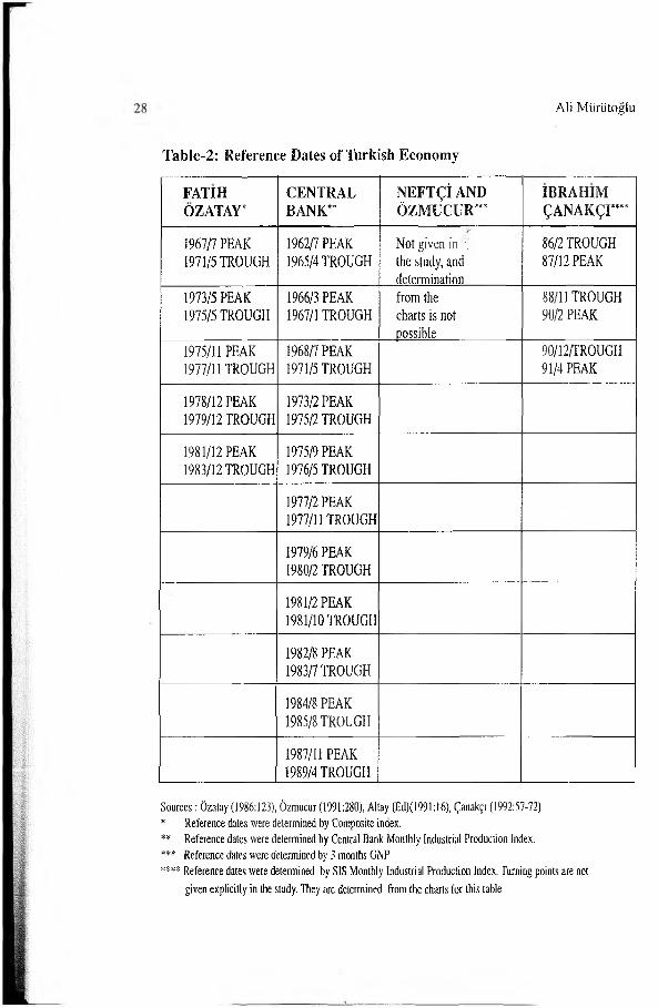
The first study on leading indicators in Turkey was made by Fatih Özatay. Özatay(1986), while searching business cycles in the Turkish economy, constructed a reference series and a leading economic indicators index for the Turkish economy. The second study on this subject was undertaken by Neftçi and Özmucur. In this study, Neftçi and Özmucur (1991) formed an Economic Condition Index (ECI) and a Leading Indicators Index (LII). They also calculated probabilities for the turning points of the cycle. Third study was made by a team within the Central Bank of the Republic of Türkiye (Altay et al., 1991). The last study about the issue was made by Çanakçı (1992). In this study, he analyzed 50 economic series from different sectors of the economy and showed that it is possible to find leading indicators for the Turkish economy. Reference dates (turning points of the cycles) of the Turkish Economy found by above studies are shown in Table-2.

Aîi Mürütoğiu

Table-2: Reference Dates of Turkish Economy

FATIHOZATAY*

CENTRALBANK**

NEFTÇİANDÖZMUCUR***

IBRAHIMÇANAKÇI”**

1967/7 PEAK 1971/5 TROUGH


Not given in •; the study, and determination

86/2 TROUGH 87/12 PEAK



from the charts is not possible

88/11 TROUGH 90/2 PEAK

1975/11 PEAK 1977/11 TROUGH


90/12/TROUGH 91/4 PEAK

1978/12 PEAK 1979/12 TROUGH


1981/12 PEAK 1983/12 TROUGH


1977/2 PEAK 1977/11 TROUGH


1981/2 PEAK 1981/10 TROUGH



1987/11 PEAK 1989/4 TROUGH

Sources: Özatay (1986:123), Özmucur (1991:280), Allay (Ed)(1991:16), Çanakçı (1992:57-72)* Reference dates were deteimined by Composite index.** Reference dates were determined by Central Bank Monthly Industrial Production Index.*** Reference dates were determined by 3 months GNP**** Reference dates were determined by SIS Monthly Industrial Production Index. Turning points are not

given explicitly in the study. They are determined from the charts for this table

v Leading Indicators Approach for Business Cylcle Forecasting and a Study on ̂ Developing a Leading Economic Indicators Index for the Turkish Economy 29

VI. A Study on Developing a Leading Economic Indicators Index for the Turkish EconomyStudies on developing leading indicators indices for the Turkish economy and the results of these studies were mentioned above. Economic series used as leading indicators should always be monitored and updated if necessary. Especially for the countries like Turkey that experiences a rapid and continuous change in its economic structure, such updates become vital. Thinking from this point of view, new leading indicators index for the Turkish Economy is developed in this section. The methodology and findings of this study are explained below:

A. Period of the Study and Definition of the Business CycleIn this study, business cycles are defined as deviations from the long run trend of the economy. Data used in this study compromises a 116 months’ time period from January 1989 to August 1998.

B. Reference SeriesWhen developing a leading indicator index, the first step is to define the reference series (cycle) and find the turning points of this series. In this study SIS (State Institute of Statistics) Monthly Industrial Production Index is used as the reference series. This index is calculated using production data of 112 basic industrial goods which compromise nearly 60% of the total industrial production. It is also calculated separately for mining, manufacturing, electricity, gas and water subsectors of the industry.

The main reason for selecting the SIS Monthly Industrial Production Index as the reference series is the assumption that fluctuations in the Turkish economy mainly reflected in the industrial sector constitutes an important part of the economy. Furthermore, the results of macro economic policy can easily be seen in the industrial sector.

C. Candidate Series for Leading Indicators IndexNearly 50 economic series from different parts of the economy are analyzed in order to develop the Leading Indicators Index.

Regarding the increasing importance of the monetary aggregate figures for the Turkish economy after 1990, series related with money and credit side of the economy are analyzed extensively. Building activities are treated as an indicator of the economic revival and series relating to the building activities, both with respect to building and occupancy permits, are taken into consideration. The number as well as capital amount

30 Ali Miirlitoglu

of newly established companies are closely related with the expectation about the economy’s future. Imports of capital goods and raw materials, in particular, are important for reflecting the future production plans of the firms. Lastly, government expenditures can be cause for a recession or revival by affecting the economy as a whole. ?

D. Decomposition of Time SeriesA time series is composed of trend, seasonal fluctuations, cycle and irregular components. Trend (T) is the long-run increase or decrease persistent in the series. Most time series show an increasing trend in the long-run. Seasonal fluctuations can be defined as movements in the series due to seasonal effects such as changes in the climate, in customs related to the year or to holidays. Irregular component (I) is the random movement that can be seen in the series. Irregular components are caused by unusual events such as war, strike, extremely adverse weather conditions etc.

These components can be combined together using two different ways depending on the characteristic of the increase in values of the series. If the value of increase in the series in the course of time is constant, the additive form is used. Accordingly, in a given time (t), the series Y(t) is expressed as follows;

Y(t) = T(t) + S(t) + C(t) + I(t)

If the increase in series is not constant but it is in proportion with the value of the series in the course of time, in other words, if the increase in the value of the series depends on the series own value, then multiplicative form is used. Accordingly, in a given time (t), the series Y(t) is expressed as follows;

Y(t) = T(t) x S(t) x C(t) x I(t)

Since the increase in economic series in the course of time is related with the series own magnitude, the multiplicative form should be used in the economic series analysis.

After defining economic time series in multiplicative form, each cycle component of the series is determined. In order to do this, other components (trend, seasonal, irregular) of the series are determined and the series is clarified from these components.

In this study, centered moving average (or seasonal index) method is


used to eliminate the seasonal effects from the series. In this method, firstly, 12-month moving averages are calculated using the monthly data. Secondly, 2-months moving averages are calculated from these averages and seasonal indexes are found for each month. Finally, monthly values of original series are divided into seasonal indices for that particular month. The resulting new series is eliminated from the seasonal component and includes only trend, cycle and irregular factors.

The least square (regression) method is used for eliminating trend components from the series. Since proportional increases are important for most economic series, a semi-logarithmic trend equation is used in the regression analysis. This equation can be expressed as:

Ln Y(t) = a + b(t) + u

Here, Y(t) shows the trend component of the series, a is the constant, t is time and u is the error term. For each series, a and b coefficients are determined using the regression analysis. Subsequently, series without seasonal components is divided by series which is calculated using the above equation in order to find the series which is eliminated from seasonal and trend factors.

The new series is eliminated from the seasonal and trend factors and only includes cycle and irregular components. 3-month moving averages are calculated in order to eliminate the irregular components. After this, the resulting series only include the cycle component. The series is standardized by subtracting each month’s value from the average of the series and divided by its standard deviation. The reason for this standardization is to make possible to the comparison of two series with different units.

E. Determining the Turning Points of the SeriesTurning points in the reference series determined by using the above methods are given in Chart 2:

32 Ali Miiriitoglu

Chart 2: SIS Monthly Industrial Production Index (Standard Values)

In the time period between January 1989-August 1998, three completed and one incomplete cycles are determined. The average length of 3 cycles is calculated as 27.4 months. Dates of the turning point in the reference series are given in Table 3:

Table 3: Dates of Turning Points for the Turkish Economy

CYCLE BEGINNINGTROUGH

PEAK TERM INALTROUGH

I 06/89 10/90 07/91II 07/91 12/93 06/94III 06/94 07/95 03/96IV 03/96 07/97 ?

F. Determining the Leading IndicatorsIn order to find leading indicators, turning points and cross correlation analyses of all series with respect to reference series are completed. In the turning point analysis, the leading time (in months) of turning points of candidate series turning points with respect to turning points of reference series are calculated. The average leading time of candidate series throughout the whole cycle is also taken into account. In order to be used as a leading indicator, the leading time of economic series should not vary


significantly while the number of cycles (turning points) in the candidate series must be equal to the number of cycles in the reference series.

For cross correlation analysis, correlation coefficients between the reference series and one, two, three...ten months lagging values of the candidate series are calculated. When determining leading indicators, series whose two, three or more months lagging values have a high correlation coefficient between the reference cycle values are selected.

Following the above analyses, nine economic series are selected as leading indicators. These series are as follows:1. Total Import of Investment Goods, in million dollar2. Total Import of Intermediate Goods, in million dollar3. Currency (in 1987 prices), billion TL4. M2 (in 1987 prices), billion TL5. Reserve Money (in 1987 prices), billion TL6. Deposit Money Banks Credits (in 1987 prices), billion TL7. Net Credit Volume (in 1987 prices), billion TL8. Consolidated Budget Monthly Expenditures (in 1987 prices), billion TL9. Total Capital of Newly Established Firms (in 1987 prices), billion TL

Leading indicators found in this study are in harmony with the finding of the previous studies. Consolidated Budget Monthly Expenditures and M2 were also taken into consideration in the TUSIAD Leading Indicators Index. Imports Volume and Total Imports of Investment Goods are in accord with the study concluded by the Central Bank. Consolidated Budget Monthly Expenditures, Net Credit Volume, Total Import of Investment Goods and M2 were also determined as leading indicators by Çanakçı.

G. Constituting the Index:The Leading Indicators Index is obtained by giving equal weight to the standard values of the above leading indicator series and adding them. In the analyzed period three completed cycle are determined as shown in Table 4.

34 Ali Miirütoglu

Table 4: Turning Points of Leading Indicators Index


PEAK TERMINALTROUGH

I 06/89 07/90 05/91II 05/91 04/93 05/94III 05/94 04/96 10/96IV 10/96 7

Following the analysis of turning points it can be said that the leading indicators index led the reference series very successfully until June 1994, but after this point, the leading power of the index has decreased slightly. However, the turning point analysis by itself is not enough to judge about the power of the leading indicators index. The relationship between the reference series and the index throughout the whole period must be also taken into account. For this purpose, both the Industrial Production Index and the Leading Indicators Index are given in Chart 3.

Chart 3 : Monthly Industrial Production and Leading Indicators Index (Standard Values)

2,00 1,50 1,00 0,50

. 0,00 - 0,50 - 1,00 ••1,50 - 2,00 - 2,50 - 3,00 - 3,50

As it can be observed from the chart, the leading indicators index is(other than a few exceptions) successful in leading the reference series.

SiS MONHTHI.Y INDUSTRIAL PRODUCTION ------ LEADING INDICATOR INDEX

H. Using the Leading Indicators Index in ForecastingThe leading indicators index is now ready for short-term forecasting of the economic activity. There are various methods for using leading indicators index in the short-mn forecasting of economic activity.1 But none of these methods give the correct forecast all the time. In addition, these methods should be considered as completing rather than competing and more than one method must be used to make the forecast more reliable.

Lastly, it must be stated that the result of the forecast of the leading indicator index should be used carefully. When making the final decision, the results of other methods should also be considered. As a fact, all methods of forecasting are only decision tools and findings of these methods should be combined with the insights and experiences of the forecaster.

VII. Summary and ConclusionIn this study, monthly data of nearly 50 economic series from different sectors are analyzed in this study in the time period between January 1989- August 1998 and 9 economic series are determined as leading indicators for the Turkish economy. These series are used to develop a Leading Indicators Index for the Turkish economy which can be used for forecasting the turning points of industrial production. In the period of analysis, three complete and one incomplete cycles are determined in the Industrial Production Index. Accordingly, June 1989, Julyl991, Junel994 and March/1996 are determined as trough dates and October 1990, December 1993, July 1995 and July 1997 are determined as peak dates of these cycles.

The leading economic series that formed the Leading Indicators Index are as follows:I. Total Import of Investment Goods, in million dollar2. Total Import of Intermediate Goods, in million dollar3. Currency (in 1987 prices), billion TL4. M2 (in 1987 prices), billion TL5. Reserve Money (in 1987 prices), billion TL6. Deposit Money Banks Credits (in 1987 prices), billion TL7. Net Credit Volume (in 1987 prices), billion TL8. Consolidated Budget Monthly Expenditures (in 1987 prices), billion TL9. Total Capital of Newly Established'Firms (in 1987 prices), billion TL


1 Interested reader can find details of these methods from the books and articles slated in the Bibliography.

34 Ali Mürütoglu

Table 4: Turning Points of Leading Indicators Index


PEAK TERM INALTROUGH

I 06/89 07/90 05/91II 05/91 04/93 05/94III 05/94 04/96 10/96IV 10/96 ?

Following the analysis of turning points it can be said that the leading indicators index led the reference series very successfully until June 1994, but after this point, the leading power of the index has decreased slightly. However, the turning point analysis by itself is not enough to judge about the power of the leading indicators index. The relationship between the reference series and the index throughout the whole period must be also taken into account. For this purpose, both the Industrial Production Index and the Leading Indicators Index are given in Chart 3.

Chart 3 : Monthly Industrial Production and Leading Indicators Index (Standard Values)

As it can be observed from the chart, the leading indicators index is(other than a few exceptions) successful in leading the reference series.


H. Using the Leading Indicators Index in ForecastingThe leading indicators index is now ready for short-term forecasting of the economic activity. There are various methods for using leading indicators index in the short-run forecasting of economic activity.1 But none of these methods give the correct forecast all the time. In addition, these methods should be considered as completing rather than competing and more than one method must be used to make the forecast more reliable.

Lastly, it must be stated that the result of the forecast of the leading indicator index should be used carefully. When making the final decision, the results of other methods should also be considered. As a fact, all methods of forecasting are only decision tools and findings of these methods should be combined with the insights and experiences of the forecaster.

VII. Summary and ConclusionIn this study, monthly data of nearly 50 economic series from different sectors are analyzed in this study in the time period between January 1989- August 1998 and 9 economic series are determined as leading indicators for the Turkish economy. These series are used to develop a Leading Indicators Index for the Turkish economy which can be used for forecasting the turning points of industrial production. In the period of analysis, three complete and one incomplete cycles are determined in the Industrial Production Index. Accordingly, June 1989, July 1991, Junel994 and March/1996 are determined as trough dates and October 1990, December 1993, July 1995 and July 1997 are determined as peak dates of these cycles.

The leading economic series that formed the Leading Indicators Index are as follows:I. Total Import of Investment Goods, in million dollar2. Total Import of Intermediate Goods, in million dollar3. Currency (in 1987 prices), billion TL4. M2 (in 1987 prices), billion TL5. Reserve Money (in 1987 prices), billion TL6. Deposit Money Banks Credits (in 1987 prices), billion TL7. Net Credit Volume (in 1987 prices), billion TL8. Consolidated Budget Monthly Expenditures (in 1987 prices), billion TL9. Total Capital of Newly Established'Firms (in 1987 prices), billion TL

1 Interested reader can find details of these methods from the books and articles stated in the Bibliography,

36 Ali Miirütoğlu

This study shows that business cycles are found in the Turkish Economy as in other developed countries’ economies and more studies should be done in the area of business cycles and leading indicators approach.

In order to make the leading indicators’ forecast more reliable and useful, some arrangement should be made. Firstly, the current values of most economic series are announced with a long time of 3-4 months delay. This hinders the power of leading indicators in forecasting. Secondly, the scope of series, in particular, the real sector of the economy, should be watched continuously and updated if necessary. Lastly, the number of surveys which shows that expectations of economic actors (firms, households etc) must be increased.

The leading indicator index should be observed in certain time periods and must be updated when necessary. Some series may be omitted from and some others may be inserted in the index. Also the techniques that are used when developing an index must also be updated in the light of new developments.

BibliographyA lta y , S ., A r ık a n , A ., B a k ır , H . v e T a ta r A ., “ L e a d in g In d ic a to rs : T h e T u rk is h

E x p e r ie n c e ” , 20. C IRETKonferansı, B u d a p e ş te , 2 -5 E k im 3991 .A n n u z ia to , P a u lo v e B a ld a s s a r r i , M a r io , e d s . , Is the Business Cycle Still Alive:

Theory, Evidence and Policies, S ( t) . M a r t i n ’s P re s s In c .,N e w Y o rk , 1 9 9 4 . A re n , S a d u n , İstihdam Para ve iktisadi Politika, 10. B a s k ı , S a v a ş Y a y ın la r ı , A n k a ra ,

1 9 9 2 .B o s c h a n C . V e E b a n k s W ., "The Phase- Average Trend, a New Way o f Measuring

Economic Growth”, P ro c e e d in g s o f th e B u s in e s s a n d E c o n o m ic S ta t is t ic s S e c t io n , A m e r ic a n S ta t is t ic a l A s s o c ia t io n , 1 9 7 8 .

B ry G . V e B o s c h a n C ., “Cyclical Analysis o f Time Series : Selected Procedures and Computer Programs”, N B E R , T e c h n ic a l P a p e r , n .2 , 1 9 7 1 .

B u rn s , A .F ., V e M i tc h e l l W .C ., Measuring Business Cycles, N B E R S tu d ie s in B u s in e s s C y c le s N o . 2 , C o lo m b ia U n iv e r s i ty P re s s , N e w Y o rk , 1946 .

Ç a n k ç ı , İ b r a h im , Kısa Vadeli Tahmin Yöntemleri ve Türkiye için Bir Deneme (Öncü Göstergeler Yaklaşımı), D P T U z m a n l ık T e z i, A n k a ra , 1992 .

D e L e e u w F. ; “ T o w a rd a T h e o ry o f L e a d in g In d ic a to r s ” , in L a h ir i K .- M o o re G .H . (e d s .) : Leading Economic Indicators, New Approaches and Forecasting Records, C a m b r id g e U n iv e r s ity P re s s , C a m b r id g e , 199 1 .

K v a n li , A . H ., G u y n e s C .S V e R o b e r t P .J , Introduction to Business Statistics, W e s t P u b lis h in g C o m p a n y , S ( t) . P a u l, 1 9 8 6 .

L a h ir i , K ., M o o re G .H ., e d . , Leading Economic Indicators, New Approaches and Forecasting Records, C a m b r id g e U n iv e r s i ty P re s s , C a m b r id g e , 1991 .

N e ftç i , S a l ih , “ O p t im a l P r e d ic t io n o f C y c lic a l D o w n tu r n s ” , Journal o f Economics Dynamics and Control, 4 , 1 9 8 2 .

N e f tç i ,S .N ., Ö z m u c u r S ., Türkiye Ekonomisi için TÜSİAD Öncü Göstergeler Endeksi, T Ü S İA D , İ s ta n b u l , 1 9 9 1 .

N e f tç i , S a l ih , “ A T im e - s e r ie s F ra m e w o rk f o r th e S tu d y o f L e a d in g in d ic a to r s ” , in L a h i r i K .- M o o re G .H . (e d s .) : Leading Economic Indicators, New Approaches and Forecasting Records, C a m b r id g e U n iv e r s i ty P re s s , C a m b r id g e , 19 9 1 .

N ie m ira , M .P ., “An International Application o f Neftçi’s Probability Approach fo r Signalling Growth Recessions and Recoveries Using Turning Point Indicators", in L a h i r i K .- M o o re G .H . (e d s .) : L e a d in g E c o n o m ic In d ic a to r s , N e w A p p r o a c h e s a n d F o r e c a s t in g R e c o rd s , C a m b r id g e U n iv e r s ity P re s s , C a m b r id g e , 1 9 9 1 .

N i l l s o n , R o n n y ., “Leading Indicators fo r OECD Central and Eastern European Countries''' in Is th e B u s in e s s C y c le S ti l l A liv e : th e o ry , e v id e n c e a n d p o l ic ie s , A n n u z ia to , P. v e B a ld a s s a r r i , M ., e d s , S ( t) . M a r t in ’s P re s s In c ., N e w Y o rk , 1 9 9 4 .

N i l ls o n , R o n n y ., OECD Leading Indicators, O E C D E c o n o m ic S tu d ie s , N o .9 ,1 9 8 7 .Ö z m u c u r , S ü le y m a n , Geleceği Tahmin Yöntemleri, İ s ta n b u l S a n a y i O d a s ı Y a y ın la r ı ,

A v c ıo l M a tb a a s ı , İ s ta n b u l , 1990 .Ö z a ta y F a t ih , Türkiye Ekonomisinde Devresel Hareketler, (A n k a ra Ü n iv e r s i te s i

S o s y a l B il im le r E n s t i tü s ü , D o k to ra T e z i) , A n k a ra , 198 6 .R ic h a r d G .L ., P e te r O .L ., D o u g la s D .P ., Economics, E ig h th E d i t io n , H a rp e r a n d R o w

P u b lis h e r , N e w Y o rk , 1 9 8 7 .S h e a r m a n , H o w a rd J . , The Business Cycle; Growht and Crisis under Capitalism,

P r in c e to n U n iv e r s i ty P re s s , O x fo rd , 1991 .Y ü k s e le r , Z a f e r , “ E k o n o m ik K o n jo n k tü r ü n D e ğ e r l e n d i r i lm e s i v e K a r ş ı la ş ı l a n

S o r u n la r ” Ekonomiyi İzleme Sempozyumu, İ s ta n b u l , 5 -6 M a y ıs 1 9 9 4Z a m o w i tz V ic to r , Business Cycles ; theory, histoıy, indicators and forecasting, T h e

U n iv e r s i ty o f C h ia g o P re s s , C h ia g o 1992 .A N K A , H a b e r B ü lte n le r i (v a r io u s i s s u e s )D e v le t İ s t a t i s t ik E n s t i tü s ü , A y lık E k o n o m ik G ö s te r g e le r (v a r io u s is s u e s )D e v le t İ s ta t i s t ik E n s t i tü s ü , A y lık İ s ta t i s t ik B ü lte n i ( v a r io u s i s s u e s )D e v le t P la n la m a T e ş k ila t ı , A y lık E k o n o m ik G ö s te r g e le r ( v a r io u s is s u e s )H a z in e v e D ış T ic a re t M ü s te ş a r l ığ ı , B a ş l ıc a E k o n o m ik G ö s te r g e le r (v a r io u s is s u e s )T ü rk iy e C u m h u r iy e t M e r k e z B a n k a s ı , A y lık B ü lte n (v a r io u s is s u e s )T ü rk iy e C u m h u r iy e t M e r k e z B a n k a s ı , Ü ç A y lık B ü lte n (v a r io u s i s s u e s )


r

38 Ali MiirutosHu

Appendix 1 : Analyzed Time Series

I. Construction1. Residential Construction (acco ding to the occupancy permits), 1000

m2 //2. Industrial Construction (according to the occupancy permit;:), 1000 m23. Commercial Construction (according to the occupancy permits),

1000 m24. Total Construction (according to the occupancy permits ), 1000 it25. Residential Construction (according to the building permits), 1000 m26. Industrial Construction (according to the building permits), 1000 m27. Commercial Construction (according to the buil^ii g permits),

1000 m28. Total Construction (according to the building permits), 1000 m2

II. Foreign Trade1. Monthly Imports, in million dollars2. Total Import of Investment Goods, in million dollars3. Total Import of Intermediate Goods, in million dollars4. Total Import of Intermediate Goods (excluding crude oil), in million

dollars5. Imports of Crude Oil, in million dollars6. Monthly Exports, in million dollars

III. Money and Credit1. Currency (in current prices), in billion TL2. Currency (in 1987 prices), in billion TL3. Monthly \verage USD Exchange Rate4. M2 (in current prices), in billion TL5. M2 (in 1987 price?), in billion TL •6. Reserve Money (in current prices), in billion TL7. Reserve Money (in 1987 prices), in billion TL8. Central Bank Credits-Public (in urrent prices), in billion TL9. Central Bank Credits-Public (in 1987 prices), in billion TL10.Central Bank Credits-Private (in current prices), in billion TL11. Central Bank Credits-Private (in-1987 prices), in billion TL12.Central Bank Credits-Total (in current prices), in billion TL13.Central BtJik Credits-Total (in 1987 prices), in billion TL14.Bank Credits (in current prices), in billion TL

Leading Indicators Approach for Business CyJcle Forecasting and a S'udy onDeveloping a Leading Economic ndicators Index for the Turkish Economy 39

15.Bank Credits (in 1987 prices), in billion TL16.Net Credit Volume (in current prices), in billion TT17.Net Credit Volume (in 198" prices), in billion TL

IV. Public Finance1. Consolidated Budget .Tonthly Revenues (in current prices), in billion TL2. Consolidated Budget Monthly Revenues (in 1987 prices), in billion TL3. Consolidated Budget Monthly Expenditures (in current prices), in

illion TL4. Consolidated Budget Monthly Expenditures (in 1987 prices),

in billion T \

V. Employment and Wages1. Manufacturing Industry Average Number of Workers, Public,

in persons2. Manufacturing Industry Average Number of Workers, Private,

in persons3. Manufacturing Indus y Average Number of Workers, Total, in persons4. Manufacturing In, ustry Average Wages , Public, in TL/hour5. Manufacturing Industry Average Wages , Private, in TL/hour6. Manufacturing Industry Average Wages , To,al, in TL/hour

VI. Investment1. Number of Capital Increased Firms, number2. Number of Newly Established Firms, number3. Number of Capital Increased + Newly Established Firms, number4. Capital of Capital Increased Firms (in current prices), in billion TL5. Capital of Capital increased Firms (in 1987 prices), in billion TL.6. Capital of Newly Established Firms (in current prices), in billion TL7. Capital of Newly Established Firms (in 1987 prices), in billion TL8. Capital of Capital Increased+Newly Established Firms (in current

prices), in billion TL9. Capital of Capital Increased + Newly Established Firms (in 1987

prices), in billion TL

VII. ISE Composite Index, month-end, close

VIII. SIS Consumer Price Index , 1987 = 100

The ISE Review Volume: 3 No: 9 January/February/March 1999 ISSN 1301-1642 © ISE 1997

CHAOS THEORY, NON-LINEAR BEHAVIOUR IN STOCK RETURNS, THIN TRADING AND

MARKET EFFICIENCY IN EMERGING MARKETS: THE CASE OF THE ISTANBUL

STOCK EXCHANGE

Alper ÖZÜN*

AbstractT h is p a p e r e x a m in e s th e w e a k fo r m e f f ic ie n c y in th e I s ta n b u l S to c k E x c h a n g e in th e p e r io d b e tw e e n 1 9 8 7 a n d 1 9 9 8 b y u s in g d a i ly IS E N a t io n a l - 100 In d e x . U n l ik e p re v io u s e m p ir ic a l p a p e r s , it e m p lo y s d i f fe re n t m e th o d o lo g ie s to ta k e a c c o u n t th e e f fe c ts o f th in t r a d in g , n o n - l in e a r b e h a v io u r in s to c k re tu r n s , c h a n g e s in th e v o la t i l i ty in th e m a rk e t a n d th e t im e -v a r ia t io n in th e m a rk e t r is k p r e m iu m . B y u s in g c h a o s th e o r y in p h y s ic s , c e r ta in g e n e ra l is e d a u to - r e g re s - s iv e m o d e ls in e c o n o m e tr ic s a n d e f f ic ie n t m a rk e t h y p o th e s is in th e f in a n c ia l th e o ry , f o r th e f i r s t t im e , w e s h o w th a t th e IS E h a s b e e n w e a k fo rm e f f ic ie n t b e tw e e n 1 9 8 7 a n d 199 8 e x c e p t f o r 1 9 9 5 a n d 1 9 9 6 in w h ic h th e re e x is ts n o n l in e a r b e h a v io u r a r is in g f r o m r i s k lo v in g a n d i r ra t io n a l b e h a v io u r o f in v e s to rs a f te r 1 9 9 4 e c o n o m ic c r is is .

I. IntroductionThis paper investigates the weak-form efficiency in the Istanbul Stock Exchange in the period between 1987 and 1998 by using daily ISE National-100 Index. Due to its short history, we witness a few papers on the efficiency of the ISE. What is more, the methodologies in those papers use the assumptions and test techniques that are valid in advanced markets, but might not be valid in the emerging markets.

Emerging markets have certain specific conditions that should be accounted in testing their informational efficiency. In this paper, we take account of effect of non-linear behaviour in stock returns and thin trading on the test of the efficiency of the ISE. We use a combination of an aug-

* Assistant Inspector, Türkiye İş Bankası, Inspection Committee, Kavakhdere-Ankara Phone: 0312 413 92 39 or 0 216 310 41 70. e-mail: [email protected]

This article is a summary of the dissertation submitted for MSc in Business Finance at Brunei University (University of West London), UK


42 Aiper Özün

mented logistic map equation for the estimation of the non-linearities in the stock returns, and an AR (1) model with adjusted returns proposed by Milier, Muthuswany and Whaley (1994) to adjustment of returns for thin trading.

In order to check if our results are sensitive to the changes in the volatility in the market that is frequently observed in emerging markets, we estimate GARCH and EG ARCH models. What is more, by following Merton (1980), a GARCH-M model suggested by Bollerslev et al., (1992) is estimated to see if the inefficiency result, if any, is due to time-variation in the market risk premium. The result is also checked by using an EGARCH-M model introduced by Nelson (1991).

In the financial literature for the first time, we find that the ISE is weak-form efficient and an attractive market for the international investors for international portfolio diversification due to its efficiency and high return.

The paper is constructed as follows: In the first part, we present a literature review on the market efficiency in emerging markets including the main papers on the efficiency of the ISE. After explaining the methodology in the second part, we present and discuss the empirical findings of our analysis in the third part. The paper ends with part 4 that includes concluding remarks and suggestions for future research.

II. Literature ReviewEfficient Market Hypothesis (EMH) asserts that financial asset prices reflect all relevant historical and current information and incorporate all forecast information in unbiased forecasts of future prices. Fama (1991) classifies empirical test of market efficiency into three categories in 1991; (I) tests for return predictability; (ii) tests for rapid price adjustments; and (iii) tests for private information.

In a weak-form efficient market in which prediction of the future return by using past values is not possible, asset prices incorporate all historical information and therefore technical analysis is useless but fundamental analysis may work. In that kind of markets, prices are memoryless, unforecastable and change only in response to the arrival of new information. In technical words, asset prices follow a random walk process according to which there is no correlation between subsequent price movements (Samuelson, 1965).

Stock prices in emerging economies move in step much more than in


advanced markeis. Emerging markets’ prices capitalise less firm specific information, and are subject to more economy-wide fluctuations.

Therefore, Samuels (1981), Drake (1985) and Kitchen (1986) argue that securities markets in developing countries are not efficient because of their operating characteristics such as size, market regulation trading costs and the nature of the investors.

Dickinson and Muragu (1994) state that given the large body of evidence on efficiency in developed markets there is a need for ‘'triangulation” in the research by providing evidence from developing markets. Triangulation can be theoretical or implemental through the use • f different research methods, different settings, different data, different assumptions and improved decision making techniques.

Morch (1998) emphasises that property rights, judicial efficiency, clean government and meaningful accounting information let stock markets process information and allocate capital better, and thus contribute to economic growth. The absence of these factors might discourage informed trading and foster noise trading.

Fast economic growth, liberalisation policies in developing markets and financial markets globalisation have provided the proper environment where equity markets could thrive. What is more, Western investors have paid attention to them due to the potentially high rates of returns offer .d by these markets.

Wood and Poshakwale (1998) argue that recent results suggest that daily returns in emerging markets violate market efficiency in the weak form. They find evidence of significant day of week effects from Kuala Lumpur stock exchange, Philippines and Italy. They argue that while account settlement procedures can particularly explain weekly returns in the Philippines, Thailand, KLSE and Germany, they do not explain the negative returns for R ondays particularly in Japan.

Flores and Szafarz (1997) test the information structure of the Warsaw Stock Exchange and refuse that the Polish Stock Exchange is informationally efficient, and microeconomic fundamentals are still absent from the WSE in spite of 772 % growth since 1993 .

Emerson, Hall and Zaiewska-Mitura (1997) test if the Bulgarian Market is becoming more efficient by using a multi-factor model with time-varying coefficients and generalised auto-regressive conditional heteroskedastic (GARCH) errors, and find varying levels of efficiency and varying speeds of movement towards efficiency.

44 Alper Özün

However, Antoniou, Ergul, Holmes (1997) argues that it is difficult to believe that the Nairobi stock market is efficient when there is evidence that some of the most developed markets in the world are characterised by inefficiency. Therefore, both the positive and negative evidence on efficiency in emerging markets may reflect the methodology adopted for testing and the time period under investigation.

Therefore, a test of market efficiency in emerging markets should take account of (i) thin trading, (ii) non-linear dependence in stock returns, and (iii) time-variation in the market risk premium.

While tests of efficiency for developed markets are characterised by high levels of liquidity, sophisticated investors with access to high quality and reliable information and few institutional impediments; in emerging markets, there are low liquidity, thin trading possibly less well informed investors with access to unreliable information and considerable volatility.

Infrequent trading of particular shares can lead to serious biases in empirical work. A major source of possible bias, according to Dickinson and Muragu (1994), is that prices recorded at the end of a time period may relate to a transaction which occurred earlier in or even prior to that period.

Miller, Muthuswamy and Whaley (1994) argue that infrequent trading introduces autocorrelation in the time series of returns for a series which would otherwise exhibit serial independence. They also suggest a methodology to remove the impact of thin trading according to which an AR(1) model is estimated from which the non-trading adjustment can be obtained.

In financial theory, it is generally assumed that all individuals are rational which implies risk aversion, unbiased forecasts and instantaneous responses to information. Their utility functions are assumed to be strictly concave and increasing. Mathematically, this implies that (I) investors always prefer more wealth to less, in other words, the marginal utility of wealth is positive, MU (W) > 0; and (ii) their marginal utility of wealth decreases as they have more and more wealth, in other words, first derivative of their marginal utility of wealth with respect to wealth is negative; dMU (W) / dW < 0. The important result of this assumption for the efficiency analysis is that prices respond linearly to new information due to rationality.

On the other hand, Fraser and MacDonald (1993) argue that in emerging markets, investors may not always display risk aversion and use

their own forecasts which introduces bias into their actions. What is more, they do not always respond instantaneously to information because either the information is not reliable or they do not have opportunity to fully analyse the information. Therefore, they might show risk loving behaviour which create non-linear behaviour in emerging market stock returns.

Therefore, as Antoniou, Ergul, and Holmes (1997) argues, if the generating process is non-linear and a linear model is used to test for efficiency, the hypothesis of random walk may be wrongly accepted because non-linear systems like chaotic ones look similar to a random walk. They conclude that conventional tests of efficiency like autocorrelation tests, run tests and frequency tests are not capable of capturing the non-linearities.

Antoniou, Ergul and Holmes (1997) list mainly five key reasons for non-linear dependence in stock returns. Firstly, because of difficulties in carrying out arbitrage transactions, the characteristics of the market microstructure might lead to nonlinearities.

Secondly, as argued originally by Costa (1994), if the feedback mechanism in price movements is non-linear, then correction is not always proportional to the amount by which the prices deviate from the asset’s real value.

Thirdly, although information arrives randomly to the market, market participants respond to that information with a lag due to the market imperfections such as transaction costs. Investors trade whenever it is economically profitable and not every time news comes to the market.

Fourthly, when announcements of important factors are made less often than the frequency of observations nonlinearities might be observed and this kind of nonlinearities may lead to a clustering of observations resulting in ARCH effects which are consistent with both efficient and inefficient pricing2.

Lastly, capital market theory assumes risk averse investors implying a linear data generating process. However, investors may be risk loving when taking a gamble in an attempt to recover their losses.

Fama and French (1992), on the other hand, argue that nonlinearities might be due to the result of time-variation in the market risk premium. Merton (1980) shows that the risk premium of the market is a function of the volatility of the market as follows:

Chaos Theory, Non-Linear Behaviour in Stock Returns, Thin Trading and MarketEfficiency in Emerging Markets: The Case of the Istanbul Stock Exchange 45

2 For instance, monthly money supply annoncements wiil cause non-linearities in daily and weekly series, but not in quarterly series.

46 Alper Özün

(1) Et-i l^m j — X^ivau-dRm]

Where Rmt is the return on the market portfolio, var¡-¡ is the variance, \ - \ is the market price of risk and Em is the expectation operator. Engle, Lilien, and Robbins (1987) and Bollerslev, Chou, ai>d Kroner (1992) show that this model can be estimated by using a GARCH-M model that allows for time variation in the conditional variance.

The econometric logic behind this model can be summarised as follows:

(2 ) Y,=Jt’xi+yhi2+Ui

Where the conditional error variance ht2 = V (u,/£2¡-i) is defined by

(3) h? = V (u,/n ,,) = e„ + ¿ 6iU2,, +X <!>ih2,.¡ + 8 w,i=l iW

where ht2 is the conditional variance of ut with respect to the information set fí,_i, and w, is a vector of predetermined variables assumed to influence the conditional error variances in addition to the past squared errors. The generalised ARCH model of Bollerslev, or GARCH (p, q), is a special case of the above equation where 8 =0; and

a n d ^(¡)ih2M iW i=l

are the MA and the AR parts of the model, respectively.

Recent research into an explanation of stock return behaviour has drawn on the field of non-linear dynamics, including cfiaos theory. Research on non-linear structure in stock returns includes the use of a bilinear model by Granger and Andersen (1978), and the bispectrum of daily returns for several common stock series by Hinich and Patterson (1985). French (1987) develops models of conditional heteroskedasticity in stock returns.

Chaos, which represents a class of non-linear deterministic as opposed to stochastic systems, has attracted attention due to its ability to produce time series sequences whose characteristics resemble phenomena observed in the market place (Benhabib, 1989, Shaffer, 1991). Although

stochastic models explain many of the fluctuations as due to external random shocks, in a chaotic system these fluctuations are internally generated as part of the deterministic process. Gilmore (1997), argues that a chaotic process also exhibits great sensitivity to small changes in the system and can produce sudden shifts in time series behaviour, along with changes in volatility.

However, there are difficulties in implementing the chaos theory to finance due to the reliability of tests that can detect chaotic behaviour. Sakai and Tokumaru (1980) show that classical autocorrelation tests can not distinguish between chaotic and random behaviour. The correlation dimension test developed by Grassberger and Procaccia (1983) in physics literature might be problematic when applied to financial series due to complexity of the methodologies employed in physics. However, the close return test developed by Mindlin and Gilmore (1992) can be applied to financial data because it works with small data sets and is robust against noise and preserve time-ordering information.

Gilmore (1997) finds that the CRSP returns exhibit nonchaotic nonlinear behaviour that cannot be fully explained by the ARCH-type models used to model non-linear structure in financial data..

Scheicher (1996) finds that returns in the Vienna Stock Exchange are non-normal and shows linear and non-linear dependence based on GARCH and Markov-Switching methods.

Following the analysis of the nonlinearity and complexity of the TOPIX data, Jasic and Poh (1998) develop dier and neural network models for predicting the TOPIX monthly changes which predict better than chance by using single-step prediction.

Hinich and Patterson (1997) ana yse the inability of investigators to make meaningful point forecasts of stock returns despite strong evidence of non-linear dependence caused by the episodic, or transient, nature of the dependencies. They develop a new methodology for detecting transient dependence in a pure white noise process that is applied to intra-day returns of a sample of stocks that are members of the Dow Jones Industrial Average.They use C test, H test, and Engle’ s LM test for ARCH/GARCH which defines another form of non-linearity used to search for transient episodes of conditional heteroskedastic volatility in daily stock returns. In this paper, however, we will use a logistic map equation, which is explained in the second chapter, due to its simplicity.

haos Theory, Non-Linear Behaviour in Stock Returns, Thin Trading and M arketfiiciency in Emerging Markets: The Case of the Istanbul Stock Exchange 47

48 Alper Özün

III. Data and Methodology

3.1. DataThis paper employs daily data on the Istanbul Stock Exchange National- 100 Index for the period July 1, 1987 to May 15, 1998 supplied by the ISE. Daily data is chosen due to the methodology employed which requires consideration of non-trading days and tests on yearly basis.

In order to decrease the volatility in the data, logarithmic values of the indices are used. What is more, the methodology employed in this paper requires use of return.

In this analysis, daily return is calculated as

(4) R,=log of indext - log of indext.}

3.2. MethodologyThis paper investigates the efficiency of the ISE by using a logistic map equation which takes account of the possibility of their being non-linearities in the price series and it has advantage over other non-linear specifications in that it can also capture the feedback mechanism.

As discussed before, non-linearities may be explained in terms of non-linear feedback mechanisms in price movements. According to this logic, if the price of an asset gets too high, self regulating mechanisms generally forces the price to down. If this feedback mechanism is not linear, it is expected that the correction will not always be proportional to the amount by which the price deviates from the asset’s fundamental value. We can explain this process by using following function:

(5) Xt = aXt.} (1- Xt.j) = aXt } - a X \}

It maps the value at time t-1 into the value at time t. XVi is a negative non-linear feedback term competing with the linear term in stabilising the series. If the correction mechanism by the market is not proportional to the deviation, the feedback mechanism might produce non-linear behaviour in financial markets. DeBondt and Thaler (1987) explain these effects by the market psychology in that investors and markets over-react to bad news and under-react to good news.

In corporate this feedback mechanism into a test methodology for efficiency in emerging markets, following equation is estimated:

(6) R, - Oo + CijRt-i 4- a n R nt-i + ut

Where Rt is the return at time t, calculated as the difference of log prices and n = 2,3. The efficient market hypothesis (EMH) requires that cco=oci=an:= 0 and ut is a white noise process. In this paper, the square and cube of returns are used as the non-linear terms.

What is more, as mentioned before, Miller, Muthuswamy and Whaley (1994) argue that thin (or infrequent) trading induces autocorrelation in the time series of returns for a series that would otherwise exhibit serial independence. They argue that a moving average model (MA) that reflects the number of non-trading days should be estimated and then returns should be adjusted accordingly in order to remove the impact of thin trading. However, since it is not easy to determine the non-trading days, they state that estimation of an AR (1) model from which the nontrading corrections can be obtained functions the same task.

In order to obtain adjusted returns, we should firstly estimate a simple random walk equation:

(7) Rt — Cl{ ■¥ &2 Rt / +

Then, adjusted returns can be obtained by using the residuals from the regression above as follows:

(8) Radi, = e, 1(1-a2)

Where Radit is the adjusted return corrected for thin trading at time tIn the light of these methodologies, this paper estimates following

models:

3.2.1. AR(1) Model:

(9) Rt — cxo + (%iRt-i Ut

A weak-form efficient market requires a 0 = oct = 0 and ut to have white-noise process. The equation shows if the first lag of the return is significant in explaining the actual return. However, this model does not account for effects of non-linear behaviour and thin trading. Therefore, this model is not appropriate to test efficiency in emerging markets which are characterised by non-linearity and thin trading.

Chaos Theory, Non-Linear Behaviour in Stock Returns, Thin Trading and M arketEfficiency in Emerging M arkets: The Case of the Istanbul Stock Exchange 49

50 Aîper Özün

3.2.2. AR (1) Model with Non-Linearities:This model, which captures non-linear behaviour in the stock returns in emerging markets, is defined as follows:

(10) R[ ~ 0({)-h CCjRf.j + OCn Ui

However, the return is not adjusted for thin trading.

3.2.3 AR (1) Model with Non-Linearities and Return Adjusted for Thin Trading:

In order to account the effects of infrequent trading upon the efficiency issue, we should estimate the logistic map equation with adjusted returns as follows:

(11) R adi< = Oo 4- a i R adjt.i + a nR n (aciJ)t.} + u,

As explained before, non-linearities might be due to the change in volatility in the market return or time-varying behaviour in the returns. In order to check the robustness of our results we will augment our results using a range of different heteroscedasticity adjusted models.

3.2.4. GARCH (1,1) Model for AR (1) with Non-Linearities and Return Adjusted for Thin Trading:

We firstly investigate if the nonlinearities, if any, are the results of changes in volatility. We estimate a GARCH (p,q) model as argued by Engle (1982) by specifying GARCH (1,1) model defined as follows:

(12) h? = VfuJQ.i) = 60 + Giu2,-} +

where ht2 is the conditional variance of ut with respect to the information set i ln .

For a well defined GARCH (1,1) process, we should have 0O >0, l(j)ikl, and 1- 0 r <Jh > 0. These restrictions ensure that the unconditional variance of ut given by V(ut) = 0o / (1-Gj- <j>i) is positive; and generally Bi is also assumed to be positive.

3.2.5. EGARCH (1,1) Model for AR (1) with Non-Linearities and Return Adjusted for Thin Trading:

We will estimate also exponential GARCH (1,1) or EGARCH (1,1) model

Chaos Theory, Non-Linear Behaviour in Stock Returns, Thin Trading and M arketEfficiency in Emerging Markets: The Case of the Istanbul Stock Exchange 51

defined as:

(13) Log h,2 = Oq -f£ 0 / ( u j hhI) + £ # /* (\u.tJ h tJ - f i j+ ^ fa lo g h 2̂ i~l i~] i - j

where jj. = E ( lut / htl), the value of ft depends on the density function assumed for the standardised disturbances, et = ut/ht. Unlike GARCH (1,1) model, EGARCH(1,1) specification has a well-defined conditional variance for all parameter values , 0O, Bi, 81*. But for the process to be stable, IcJjjk 1 is still needed.

3.2.6. GARCH-M (1,1) Model for AR (1) Model with Non-Linearities and Return Adjusted for Thin Trading:

More importantly, in order to check if the nonlinearities are due to change in the time-variation in the returns, we estimate a GARCH-in mean model, mainly GARCH-M (1,1) as suggested by Merton (1980), Engle, Lilien and Robbins (1987), and Bollerslev, Chou, and Kroner (1992) as follows:

(14) Rad]t = ao + Xh2t OhRadjt-i + a t,R" + u,

(15) h2t = b(} + biu2t-]+b2 ht.i

where h{ is the conditional variance and ut is the error term.

3.2.7. EGARCH-M (1,1) Model for AR (1) with Non-Linearities and Return Adjusted for Thin Trading:

Nelson (1991), on the other hand, argues that it is often the case that the conditional variance, h2t, is not an even function of the past disturbances, ut-i, ut-2,... The exponential GARCH in mean (EGARCH-M) model aims at capturing this behaviour that is often observed when analysing stock market returns. Following Nelson (1991) we estimate EGARCH-M (1,1) models as follow:

(16) Rad>t = ao + Xh2t 0L1 Radjt-i + a nRn(adj)t-j + ut

(17) h2t =b0 + biu2(.i+b2 h,.}

In this model, h2t has the following exponential functional form:

(18) Log h 2 = Qo+0} (ut-il ht.i)+6* (! ut.} / htJ-jij+fylogh2̂ }

52 A lper Özün

where |i = E (lut / htl), the value of |a depends on the density function assumed for the standardised disturbances, et - u,/ht.

Unlike the GARCH-M model, the EGARCH-M model always yields a positive conditional variance for any choice of unknown parameters.

IV. Empirical FindingsBefore starting econometric analysis, the prima-facie evidence from TABLE-1 gives a general idea about the evolution of the ISE. The value of trading rose from $123 million in 1987 to $ 58,104 million in 1997 and 42,284 as of July 1998. Accordingly, the mean of the index rose from 930 in 1987 to 204,737 in 1997 and it is 3557(00) as of July 1998.

Table I: Yearly Trade Values, Mean and Standard Deviation of the Index

Year Value of Trading Mean of Standard Deviation(in $ million) Index of Index

1987 118 930 1891988 115 530 1301989 773 904 5011990 5, 854 4,017 7131991 8, 502 3,715 7081992 8, 567 3,992 3881993 21,770 10,558 4,5961994 23, 203 21,799 4,6841995 52, 357 41,807 8,3091996 37, 737 68,383 12,5471997 58, 104 204,737 65,16719983 42, 284 3,557 399

It is obvious from the dramatical change in the numbers that the changes in regulations and liberalisation of the market have increased interest in the equity market. Further evidence of the maturing of the market can be observed in the following table:

3 Index has been divided by 1,000 since 1998.

Chaos Theory, N on-Linear Behaviour in Stock Returns, Thin Trading and M arketEfficiency in Emerging M arkets: The Case of the Istanbul Stock Exchange 53

Table-2 ISE Historical Values

Year T. Traded Daily Traded Total stock Average Stock Contracts ContractsValue Value Traded TVaded- Total Daily

($ million) ($ million) (million) Daily (‘000) (‘000)1987 118 - 15 - NC NC1988 115 - 32 - 112 -

1989 773 3 238 1 247 11990 5, 854 24 1,537 6 766 31991 8,502 34 4, 531 18 1, 446 61992 8, 567 34 10, 285 41 1,681 71993 21, 770 88 35, 249 143 2,815 111994 23, 203 92 100, 062 396 5, 085 201995 52, 357 209 306, 254 1,220 11,667 461996 37, 737 153 390,917 1, 583 12, 446 501997 58, 104 231 919, 784 3, 650 17, 639 701998-July 42, 284 349 816, 242 6, 746 11, 129 92

However, examination of the standard deviation of the market, which might be taken as a measure of volatility and riskiness of the market, shows that volatility in the return is parallel to the increase in the mean of index except for 1992 and 1998. Main reason for the volatility in the index might be political and economic instability in the country.

54 A i per Özün

Table-3 Rt ~ (Xo + cîj Rt-i *i*

YEAR a 0 ai m i ) 1 X2(l)2 X2(l)3

19.45*1987 -0.001(-0.54)4

0.429(3.23)*

0.26 4.93*+

1988 -0.002(-1.26)

0.200(2.16)*

0.20 2.69 30.75*

1989 0.004(2.49)*

0.345(4.41)*

9.03* 2,21 6,30*

1990 0.001(0.48)

0.330(4.38)*

1.71 0.41 7.86*

1991 0.001 . (0.50)

0.083(0.93)

5.29* 0.93 30.93*

1992 -0.305E-3(-0.21)

0.131(2.08)*

2.91 0.05 0.26

1993 0.006(3.55)*

0.078(1.22)

1.50 0.03 0.10

1994 0.626E-3(0.29)

0.367(5.49)*

4.54* 1.06 4.32*

1995 ' 0.002 (0.92)

0.017(0.27)

9.57* 4.43* 0.01

1996 0.003(2.47)*

0.87(1.37)

0.02 3.92* 0.02

1997 0.004(2.26)*

0.161(1.46)

0.56 2.13 50.31*

1998 -0.052(-0.98)

-0.013(-0.12)

34.68* 0.05 ; 0.01

Figures in parentheses are t statistics* denotes statistically significant at 5 % level of significance

** denotes statistically significant at 10 % level of significance1 denotes lagrange multiplier X2 test for residual serial correlation2 denotes Ramsey’s RESET X2 test for functional form3 denotes X2 test for heleroscedasticity+ By following the LSE tradition we use 3.50 as a critical t value for all misspecification tests

J In presence of homoscedasticity, all t-rations are based on White's heteroscedasticity adjusted standard errors.

Chaos Theory, Non-Linear Behaviour in Stock Returns, Thin Trading and MarketEfficiency in Emerging Markets: The Case of the Istanbul Stock Exchange 55

However, the crucial question with respect to resource allocation is whether the changes in the regulations, non-linearities and thin trading have affected the efficient functioning of the market.

Table 3 shows the result for AR (1) model on yearly basis, As table displays early years of the time series of ISE return require rejection of a simple random walk model, thus acceptance of inefficient pricing, What is more, the diagnostic tests show that the hypothesis that the error term is a white noise process is rejected. Specifically, the series is found to be serially correlated and there is a clear presence of heteroscedasticity for almost all years except for 1992 and 1993. However, after 1992, in which there were remarkable change in regulations as explained before, the first lags of the returns are statistically insignificant except for 1994, where there was a serious crisis in the economy.

Table 4a examines an AR (1) model with non-linearities, mainly the square values of the returns. Although itself it is not significant except for 1987, 1995 and 1996, the introduction of the square of the return in the simple random walk equation leads to the error term having white noise properties for most years. However, we can not accept the random walk model except for 1991 and 1998 since either Oo oti or ocn is statistically significant. This again implies predictability and rejection of weak form efficiency.

56 A lper Özün

Table-4a Rt = oco+ «i Rt-ı + « n RVı + ut (n=2)

YEAR cx0 «I an X2(l y X2(l y X2(l)31987 -0.004

(-1.49)0.429(5.25)*

2.949(2.24)*

0,01 0.01 1.03

1988 -0.003(-1.92)**

0.206(2.35)*

2.084(1.00)

1.14 16.65* 6.97*

1989 0.003(1.54)

0.324(5.34)*

1.828(1.49)

10.83* 0.04 2.61

1990 0.925E-4(0,038)

0.331(4.44)*

0.666(0.48)

1.15 3.86* 6.11*

1991 -0.16E-3(-0.07)

0.068(0.79)

1.049(0.65)

1.31 5.90* 28.22*

1992 -0.39E-3(-0.25)

0.133(2.10)*

0.274(0.21)

2.50 6.58* 0.53

1993 0.006(3.24)*

0.081(1.23)

-0.222(-0.17)

1.61 1.25 0.05

1994 0.002(0.82)

0.362(6.14)*

-1.112(-1.03)

6.18* 3.32 2.21

1995 -0.53]B-3(-0.28)

0.052(0.80)

2.964(2.11)*

3.60* 0.16 0.50E-3

1996 0.002(1.39)

0.021(0.30)

3.405(1.98)*

0.02 0.41 0.01

1997 0.005(2.62)*

0.163(2.62)*

-1.369(-1.46)

1.05 0.41 3.03

1998 -0.052(-0.98)

0.390(0.21)

0.089(0.22)

11.89* 0.24 0.01

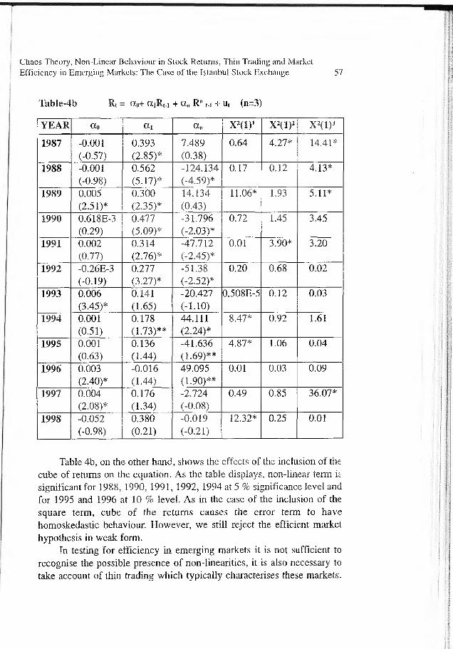
Chaos Theory, N on-Linear Behaviour in Stock Returns, Thin Trading and MarketEfficiency in Emerging M arkets: The Case of the Istanbul Stock Exchange 57

Table-4b Rt = a<>+ aiRt-i + a„ Rn t.i + ut (n=3)

YEAR OCo Cti 0!,n x2(iy X2( l)2 X 2( l )3

1987 -0.001(-0.57)

0.393(2.85)*

7.489(0.38)

0.64 4.27* 14.41*

1988 -0.001(-0.98)

0.562(5.17)*

-124.134(-4.59)*

0.17 0.12 4.13*

1989 0.005(2.51)*

0.300(2.35)*

14.134(0.43)

11.06* 1.93 5.11*

1990 0.618E-3(0.29)

0.477(5.09)*

-31.796(-2.03)*

0.72 1.45 3.45

1991 0.002(0.77)

0.314(2.76)*

-47.712(-2.45)*

0.01 3.90* 3.20

1992 -0.26E-3(-0.19)

0.277(3.27)*

-51.38(-2.52)*

0.20 0.68 0.02

1993 0.006(3.45)*

0.141(1.65)

-20.427(-1.10)

0.508E-5 0.12 0.03

1994 0.001(0.51)

0.178(1.73)**

44.111(2.24)*

8.47* 0.92 1.61

1995 0.001(0.63)

0.136(1.44)

-41.636(1.69)**

4.87* 1.06 0.04

1996 0.003(2.40)*

-0.016(1.44)

49,095(1.90)**

0.01 0.03 0.09

1997 0.004(2.08)*

0.176(1.34)

-2.724(-0.08)

0.49 0.85 36.07*

1998 -0.052(-0.98)

0.380(0.21)

-0.019(-0 .21)

12.32* 0.25 0.01

Table 4b, on the other hand, shows the effects of the inclusion of the cube of returns on the equation. As the table displays, non-linear term is significant for 1988, 1990, 1991, 1992, 1994 at 5 % significance level and for 1995 and 1996 at 10 % level. As in the case of the inclusion of the square term, cube of the returns causes the error term to have homoskedastic behaviour. However, we still reject the efficient market hypothesis in weak form.

In testing for efficiency in emerging markets it is not sufficient to recognise the possible presence of non-linearities, it is also necessary to take account of thin trading which typically characterises these markets.

58 Alper Özün

Thin trading leads to serial correlation. Therefore, observed dependence is not necessarily evidence of predictability, but might be a result of statistical illusion due to thin trading.

As presented on Table 5a, logistic map equation with adjusted returns shows that the ISE National-100 Index tends io be weak-form efficient as a result using of adjusted returns for thin trading. Efficiency requires CXo ~ 0Ci= a„= 0 and error term having white noise properties. Inclusion of the square of returns into AR (1) model with adjusted returns cause first lag of the adjusted returns to be statistically insignificant from zero except for 1990, although in some years the coefficient of the constant term is significantly different from zero. What is more, the effect of thin trading can be clearly observed in this analysis: using adjusted returns for thin trading instead of simple returns leads error térms to be serially uncorrelated except for 1989.

Another important finding of this analysis is that non-linear term in the equation is significant for 1995 and 1996. Nonlinearities in these years might be result of risk loving behaviour of the investors after 1994 crisis. We estimate an AR (1) model with non-linearities and returns for thin trading using cubic terms, as well.

Chaos Theory, Non-Linear Behaviour in Stock Returns. Thin Trading and MarketEfficiency in Emerging Markets: The Case of the Istanbul Stock Exchange 59

Table-5a Radjt = a 0 + a iR adVi +ccnRn (adj)t-i + ut (n=2)

YEAR «0 a i a n x 2U )‘ X2( l )2 X2( l )3

1987 0,019(0.51)

2.129(1.19)

2.512(1.17)

1.10 3.44 4.76*

1988 -0.124(-1.45)

0.768(0,88)

1.925(0.861)

0.29 4.58* 19.87*

1989 -0.362(2.35)*

-0.16(-0.18)

-0.327(-0.25)

4.71* 0.30 1.62

1990 -0.242(-1.39)

0.507(0,49)

0.722(0.46)

1.28 6.07* 4.19*

1991 -0.076(-5.97)*

0.192(0.69)

1.140(0.72)

0.01 0.82 24.03*

1992 -0.120(-4.82)*

0.151(0.41)

0.514(0.37)

0.23 5.45* 1.96

1993 -0.923(-1.16)

-0.368(-0,18)

-0.239(-0.184)

0.55 None 0.01

1994 -0.556(-3.27)*

-1.079(-1.17)

-1.527(-1.23)

0.64 0.01 1.23

1995 -0.017(“8.97)

0.127(1.40)

2.807(2.05)*

0.14 0.42 1.96

1996 -0.064(-5.39)*

0.606(2 .12)*

3.73(2.17)*

0.04 0.22 0,44

1997 -0.089(-4.25)*

-0.168(-0.38)

-0.984(-0.44)

0.09 3.84* 34.15*

1998 0.055(7.27)*

0.156(1.51)

0.03(1-40)

0.01 0.31 0.76

60 Alper Özün

Table-5b Radjt = cxo + aıRatJVı +a„Rn (adiVı + u( (n=3)

YEAR ao ai a« x 2(i y X2(l)2 X2(l)3

1987 -0.142(-0.76)

1.020(1.53)

-1.877(-1.52)

1.40 3.43 5.21*

1988 -0.135(-3.44)*

0.495(1.70)**

-4.070(-1.72)**

0.64 7.62* 18.79*

1989 -0.345(-3.29)*

-0.03(-0.6)

0.259(0.21)

3.29 -0.06 0.21

1990 -0.258(-2.25)*

0.316(0.62)

-0;861(-0.58)

1.39 3.69* 4.57*

1991 -0.075(-6.69)*

0.157(0.92)

-6.201(-1.11)

0.17 2.52 19.18*

1992 -0.118(-6.56)*

0.144(0.74)

-2.340(-0.71)

0.05 1.16 1.38

1993 -0.855(-1.62)

-0.143(-0.14)

0.081(0.15)

0.55 0.03 0.01

1994 -0.494(-4.30)*

-0.543(-1.17)

1.434(1-29)

0.61 0.01 1.14

1995 -0.016(-8.22)*

0.120(1.34)

-28.460(-2.03)*

0.03 0.44 3.12

1996 -0.070(-6.84)*

0.336(1.90)**

-15.55(-2.04)*

0.06 1.12 0.53

1997 -0.086(-5.46)*

-0.072(-0.30)

2.773(0.4)

0.02 2.52 27.83*

1998 0.055(7.17)*

0.162(1.51)

0.008(-1.41)

0.589E-3 0.25 0.74

The non-linear term is statistically significant in 1988 (at 10% significance level), 1995 and 1996 (at 5% significance level), and first lag of the daily adjusted returns is significantly different from zero in 1988 and 1996 at 10 % significance level.

We have reached mainly the same results; inclusion of the adjusted returns into the simple augmented logistic map equation causes error terms to have white noise properties and non-linear terms to be statistically insignificant from zero except for 1995 and 1996 in which market could be characterised by irrational and risk loving investors after 1994 economic crisis.

Chaos Theory, Non-Linear Behaviour in Stock Returns, Thin Trading and M arketEfficiency in Emerging Markets: The Case o f the Istanbul Stock Exchange 61

However, as explained before, nonlinearities found in table 5a and 5b might be the results of (i) changes in volatility and/or (ii) time variation in the risk premium.

Firstly, we determine whether the findings of non-linearities are the results of changes in volatility by estimating GARCH (1,1).

As Table 6a displays, the first lag of the squared adjusted returns in1995 and 1996 is still statistically significant at 10 % significance level.

Table-6a GARCH (1,1) Model5 (n=2)

YEAR oto OCl 0Cn

19871988 -16.504 0.323 0.717

(-2.00)* (0.39) (0.35)1989 -19.176 0.875 1.225

(-0.95) (0.75) (0.73)1990 -9.933 1.304 1.824

(-0.60) (1.30) (1.20)1991 -S.066 0.105 0.517

(-7.61)* (0.43) (0.36)1992 -12.959 0.035 0.177

(-4.52)* (0.08) (0.11)1993 -8.989 0.208 0.837

(-5.84) (0.72) (0.61)1994 -41.840 -0.148 -0.026

(-2.07)* (-0.14) (-0.02)1995 -1.589 0.143 2.657

(-8.38)* (1.55) (1.71)**1996 -6.402 0.620 3.790

(-4.39)* (1.79)** (1.85)**1997 -17.511 -0.139 -0.327

(-4.182)* (-0.27) (-0.21)1998

5 In 1987 and 1998 there are convergence problems in all GARCH models probably due to improper initial values used by Microfit4. Although we have changed initial values as suggested in the Microfit Manual, we have not been able to converge our estimations. The problem exits also for EGARCH model in 1993 and 1994, However, this does not affect either the aim nor the result of this paper.

62 Alper özün

Table™ 6b GARCH (1,1) Model (n=3)

YEAR OCo a i a„

19871988 -16.555 0.247 -1.751

(-2.94)* (0.59) (-0.51)1989 -20.124 0.620 -1.641

(-1.47) (1.05) (-1.01)1990 -16.579 0.698 -1.818

(-1.48) (1.38) (-1.21)1991 -7.934 0.107 -3.817

(-8.59)* (0.72) (-0.65)1992 -12.543 0.071 -1.534

(-6.32)* (0.33) (-0.40)1993 -8.970 0.165 -3.788

(-7.87)* (1.09) (-0.94)1994 -43.015 -0.192 0.153

(-3.17)* (-0.35) (0.11)1995 -1.491 0.135 -29.456

(-7.80)* (1.54) (-1.71)**1996 -7.088 0.327 -15.227

(-5.87)* (1.57) (-1.70)**1997 -16.909 -0.056 0.287

(-5.94)* (-0.22) (0.10)1998

Results on the Table 6b also shows that first lag of the cube of the adjusted returns in 1995 and 1996 is significant at 10 % level while the non-linear term in 1988 is found statistically significant at 10 % level in table 8b is determined insignificant in GARCH (1,1) model.

The results found by GARCH (1,1) model show that the non-linear terms in 1995 and 1996 are not due to volatility changes, while in 1988, the non-linear term might be due to the changes in volatility.

As certain problems arise with ARCH and GARCH processes such as presence of negative conditional variance and non-stationarity in the series, we also repeat the same procedure by using EGARCH (1,1) model as explained in the methodology part.

As Table 7a shows, there exits statistically significant non-linear

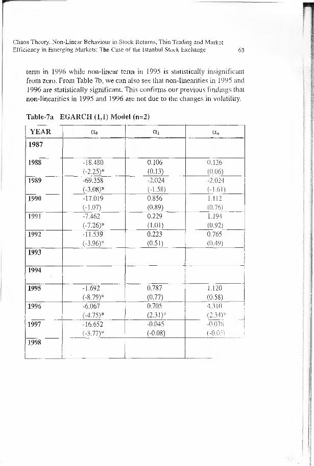
Chaos Theory, N on-Linear Behaviour in Slock Returns, Thin Trading and M arketEfficiency in Emerging Markets: The Case o f the Istanbul Stock Exchange 63

term in 1996 while non-linear te rn in 1995 is statistically insignificant from zero. From Table 7b, we can also see that non-linearities in 1995 and1996 are statistically significant. This confirms our previous findings that non-linearities in 1995 and 1996 are not due to the changes in volatility.

Table-7a EGARCH (1,1) Model (n=2)

YEAR a 0 ai a«

1987

1988 -18.480 0.106 0.126(-2.25)* (0.13) (0.06)

1989 -69.358 -2.024 -2.024(-3,08)* (-1.58) (-1.61)

1990 -17.019 0.856 1.112M.07) (0.89) (0.76)

1991 -7.462 0.229 1.194(-7.26)* (1.01) (0.92)

1992 -11.539 0.223 0.765(-3.96)* (0.51) (0.49)

1993

1994

1995 -1.692 0.787 1.120(-8.79)* (0.77) (0.58)

1996 -6.067 0.705 4.310('4.75)* (2.31)* (2.34)*

1997 -16.652 -0.045 -0.078(-3.77)* (-0.08) (-0.05) !

1998

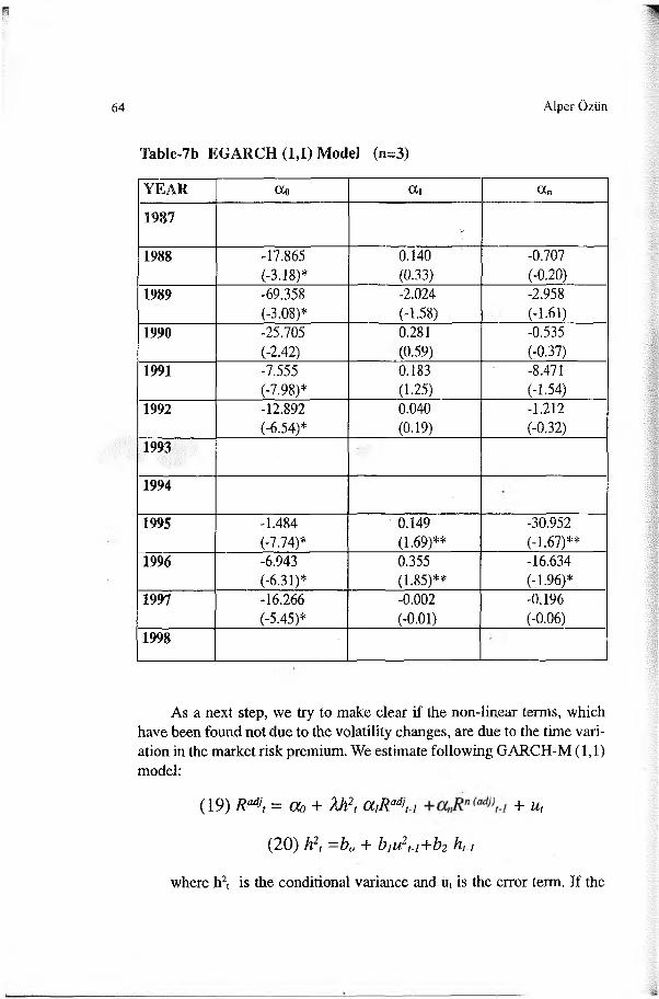
64 A lper Özün

Table-7b EGARCH (1,1) Model (n=3)

YEAR (Xo Oil a„

1987/

1988 -17.865 0.140 -0.707(-3.18)* (0.33) (-0.20)

1989 -69.358 -2.024 -2.958 .(-3.08)* (-1.58) (-1.61)

1990 -25.705 0.281 -0.535(-2.42) (0.59) (-0.37)

1991 -7.555 0.183 -8.471(-7.98)* (1.25) (-1.54)

1992 -12.892 0.040 -1.212(-6.54)* (0.19) (-0.32)

1993

1994

1995 -1.484 0.149 -30.952(-7.74)* (1.69)** (-1.67)**

1996 -6.943 0.355 -16.634(-6.31)* (1.85)** (-1.96)*

1997 -16.266 -0.002 -0.196(-5.45)* (-0.01) (-0.06)

1998

As a next step, we try to make clear if the non-linear terms, which have been found not due to the volatility changes, are due to the time variation in the market risk premium. We estimate following GARCH-M (1,1) model:

(19) Radi, = do + Xh2, a ,R adi, i + u,

(20) h2, =b„ + b,u2,.,+b2 h,.,

where h2t is the conditional variance and ut is the error term. If the

pattern of the results identified above is not due to time-varying risk premia, Oo, oti, and a n should be statistically significant for 1995 and 1996.

Tables 8a and 8b display an interesting result: Inclusion of the conditional variance into the AR (1) model with non-linearities and returns adjusted for thin trading has caused both non-linear terms and first lag of the adjusted returns to be statistically insignificant from zero. Therefore, this finding argues that predictability in 1995 and 1996 is due to the risk- retum relationship rather than inefficient pricing. Market is efficient, and inefficiency is a misleading finding resulting from time-variation in the market risk premium as Merton (1980) suggests.

However, the coefficients of the parameters for 1995 and 1996 in tables 8a and 8b, which are near to the critical t-value of 1.645 at 10 % significance level, encourage us to estimate the model by using also EGARCH-M specification for 1995 and 1996.

As explained before, EGARCH-M model proposed by Nelson (1991) allows for the positive asymmetric effects of past errors on the conditional error variances and always yields a positive conditional variance. Using of the squared and cubed terms in our analysis also encouraged us to employ EGARCH-M model.

Chaos Theory, Non-Linear Behaviour in Stock Returns, Thin Trading and M arketEfficiency in Emerging Markets: The Case o f the Istanbul Stock Exchange 65

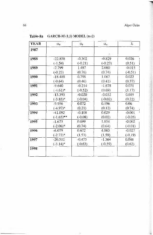
A lper Özün

Table-8a GARCH-M (1,1) MODEL (n=2)

YEAR «0 «1 a n X

1987

1988 -22.858 -0.302 -0.829 0.026(-1.54) (-0.21) (-0.23) (0.51)

1989 -7.799 1.497 2.080 -0.015(-0.23) (0.76) (0.74) (-0.51)

1990 -18.488 0.798 1.067 0.022(-0.64) (0.46) (0.41) (0.37)

1991 -9.640 -0.214 . -1.678 0.071(-4.61)* (-0.52) (0.69) (1.17)

1992 -13.393 -0.020 -0.032 0.019(-3.85)* (-0.04) (-0 .02) (0.22)

1993 -9.956 0.072 0.196 0.06(-4.97)* (0.21) (0 .12) (0.74)

1994 -41.092 -0.108 0.029 -0.001(-1.65)** (-0.08) (0.02) (-0.05)

19 95 -1.673 0.099 1.854 -0.002(-2.06)* (0.74) (0.64) (-0 .01)

1996 -6.079 0.672 4.083 -0.027(-2.72)* (1.53) (1.59) (-0.19)

1997 -20.502 -0.475 -1.364 0.046(-3.14)* (-0.63) (-0.59) (0.62)

1998

Chaos Theory, N on-Linear Behaviour in Stock Returns, Thin Trading and M arketEfficiency in Emerging Markets: The Case o f the Istanbul Stock Exchange 67

Table-8b GARCH-M (1,1) MODEL (n=3)

YEAR oc« OCi a n X

1987

1988 -18.764 0.085 -0.442 0.013(-1.82)** (0.11) (-0.07) (0.25)

1989 -17.539 0.731 -1.941 -0.006(-0.75) (0.73) (-0.71) (-0.20)

1990 -21.946 0.462 -1.105 0.021(-1.20) (0.58) (-0.45) (0.38)

1991 -9.820 -0.140 6.236 0.061(-3.24)* (-0.35) (0.38) (0.74)

1992 -12.62 0.064 -1.412 0.005(-5.25)* (0.26) (-0.32) (0.06)

1993 -9.513 0.117 -2.481 0.045(-6.42)* (0.67) (-0.54) (0.57)

1994 -43.324 -0.204 0.183 0.928 IE-3(-2.58)* (-0.30) (0.11) (0.03)

1995 -1.517 0.134 -29.170 0.004(-1.57) (1.41) (-1-43) (0.03)

1996 -6.976 0.339 -15.734 -0.011(-3.75)* (1.30) (-1.43) (-0.08)

1997 -18.696 -0.197 2.046 0.039(-4.19)* (-0.53) (0.46) (0.53)

1998

Tables 9a and table 9b display the results of EGARCH-M (1,1) specification for AR (1) model with squared and cubic non-linear returns, respectively, and adjusted for thin trading in 1995 and 1996,

68 Aiper Özün

Table- 9a EGARCH-M (1,1) Model (n=2)

YEAR OCo «1 OCn %1995 -0.674 0.159 4.437 -0.172

(-1.06) (1.66)** (! .98)* (-1.42)1996 -4.922 0.889 5.603 -0.148

(-2.80)* (2.51)* (2.42)* (-0.79)

Table- 9b EGARCH-M (1,1) Model (n=3)

YEAR a 0 OCl a„ X

1985 -0.972 0.160 -40.441 -0.086(-3.45)* (1.82)** (-1.97)* (-2.29)*

1996 -5.808 0.479 -23.578 -0.147(-3.35)* (2.04)* (-1.92)** (-0.73)

As expected, by employing EGARCH-M model instead of GARCH-M model, we find out that both inefficiency and nonlinearities founded in Tables 5a and 5b are not due to the time-varying behaviour of the returns. Both constant, first lag of the adjusted returns and non-linear terms are statistically significant which suggest predictability due to inefficient pricing rather than time-variation in the risk premium.

Y. Concluding Remarks and Suggestions for Future ResearchThis paper takes account of effects of non-linear behaviour in stock returns and thin trading on the test of the efficiency of the ISE National- 100 Index. We combine an augmented logistic map equation which considers non-linearity in the returns and an AR(1) model suggested by Miller, Muthuswany and Whaley (1994) from which the non-trading adjustment can be obtained easily. We estimate the models on yearly basis to show the development in the market.

The results of an AR (1) model displays that in its early years, the ISE was characterised by inefficient pricing. Specifically, constant term and first lag of the daily returns are statistically significant and the error term does not have white noise properties for most years up to 1992. However, since 1993, probably due to the remarkable liberalisation and changes in the regulations, the market seems to be efficient.

The results of an AR (1) model with non-linearities show that in some years, non-linear terms are significant. Market participants display irrational, risk loving behaviour, which is reflected itself as non-linearity in market returns.

When we re-estimate our model with returns adjusted for thin trading, on the other hand, we reach an interesting conclusion; the first lag of the adjusted returns have become statistically insignificant from zero, and error terms have been serially uncorrelated. Due to thin trading, prices recorded at the end of a time period have a tendency to represent an outcome of a transaction that occurred earlier in, or prior to, the period in question. Thus, adjusted returns in the equation have caused the time series to exhibit serial independence.

After finding our main results, we checked if the non-linear behaviour in stock return in 1995 and 1996 was due to the changes in the volatility in the market. However, by using GARCH and EG ARCH models, we were able to show that non-linearities are due to the inefficient pricing rather than changes in volatility.

Another possible reason for the predictability in 1995 and 1996 could be a result of time-variation in the market risk premium rather than risk-retum relationship. By using GARCH-M model, we found that predictability in those years were due to the time-variation in the market risk premium. By following Nelson (1991) we estimated EGARCH-M model for those years and found that inefficiency result for 1995 and 1996 were not due to the time-varying behaviour of the returns but inefficient pricing. After 1994 crisis, investors showed irrational and risk-loving behaviour which caused inefficient pricing in the market, and reflect itself as non-linear behaviour in the stock returns which are out of changes in volatility or time-variation in market risk premium.

The importance of this paper for the efficiency of the ISE is that for the first time, except for the work by Antoniou, Ergul, and Holmes (1997), which investigates 1988-1993 period, the ISE has been found informationally weak-form efficient after required “triangulations” in the methodology.

The result in this paper has two important implications:Firstly it has been showed again that test of market efficiency in

emerging markets requires different assumptions and methodologies and the result depends on the methodology employed. Due to the special conditions in emerging markets, it is possible to reject the efficient market hypothesis by using methodologies whose assumptions are valid in

Jhaos Theory, Non-Linear Behaviour in Stock Returns, Thin Trading and M arkeiEfficiency in Em erging M arkets: The Case of the Istanbul Stock Exchange 69.

70 Alper Özün

mature markets.Secondly, despite of the political instability and risk, Turkish finan

cial market is enough strong to allocate the resources efficiently. Investors may not develop profitable trading strategies by using historical values of the index. Technical analysis does not work in the ISE. In other words, it is not possible for the investment professionals to construct portfolios for investors by meeting their individual prefe ences and tolerance for risk.

This pragmatic result has an important implicatio i for international investors and international portfolio diversification. Akdoğan and Akdoğan (1996) fail to accept the hypothesis that the ISE is integrate 1 to a benchmark international capital market. They argue that local exchange in Turkey does not offer premium for international sources of systematic risk and the assets are priced as if the market is segmented from the rest of the world. Therefore, as a weak-form efficient and segmented market, the ISE gives international investors the chance to decrease the non-diver- sifable risk in their portfolios with high return.

Finally, it shruld be emphasised that future research on the test of efficiency in emerging markets should concentrate on the new methodologies which properly reflect the conditions in emerging markets into testable methodologies. What is more, due to the market specific conditions, even each emerging market may require different testing approaches. In that respect, a marriage of financial theory to chaos theory and physics seems to be desirable for the reflection of the complex processes in the emerging markets into econometrics tests.

ReferencesAlexakis, P.& Xanthakis, M., “Day o f the Week Effect on the Greek Stock Market”,

Applied Financial Economics, Vol. 5, 1995, 43-50 Antoniou, A. & Ergul, N. & Holmes, P., “Market Efficiency, Thin Trading and Non-Linear

Behaviour: Evidence from an Em erging Market”, European Financial Management, Vol.3, 1997, pp. 175-88.

Aydoğan, K..& Muradoglu, G. “Do Markets Learn from E perience? Price Reaction to Stock Dividends in the Turkish Market”, Discussion Paper No: 9416-C, Department of Management, Biikent University, Ankara, 1994

Balaban, E., “Informational Efficiency o f the Istanbul Securities Exchange and Some Rationale for Public Regulation”, Discussion Paper No: 9502, Central Bank of Türkiye, 1995

Balaban, E.& Bulu, “Monthly Effects in an Emerging Stock Market”, Unpublished Paper, Research Department, Central Bank of Türkiye, 1995

Balaban, E.& Candemir, H.B., “Istanbul Menkul Kıymetler Borsası’nda Bahama Etkileri”, İşletme ve Finans, vol. 113, 1995, pp. 93-104

Balaban, E.& Candemir, H.B.& Kunter, K., “Istanbul Menkul Kıymetler Borsası’nda

C ,aos Theory, N on-Linear Behaviour in Stock Returns, Thin Trading and M arketEffi iei cy in Emerging Markets: The Case of the Istanbul Stock Exchange 71

Yarıgüçlü Etkinlik”, Sermaye Piyasası Kurulu Yayını, 1995 Ball, R.& Kothar', S.R, “Nonstationary Expected Returns: Implications for Tests of

Market Efficiency and Serial Cos.elation in Returns”, Journal of Financial Economics, Vol. 25, 1989, pp. 5İ-74

Boabang, F., “An Adjustment Procedure for Predicting Betas When Thin Trading is Present: Canadian Evidence”, Journal o f Business Finance and Accounting, Vol. 23 (9&10), December 1996, pp. 1333-57

Buckberg, E., “Emerging Stock Markets and International Asset Pricing” The World Bank Economic Review, Vol.9, 1995, pp. 51-74

Butler, K.C.& Maiaikah, S.J., “Efficiency and Inefficiency in Thinly Traded Stock Markets: Kuwait and Saudi Arabia”, Journal of Banking and Finance, Vol. 16, 1992, pp. 197-210

Chopra, N.J. & Lakanishok, J.& Ritter, J.R., “Measuring Abnormal Performance: Do Stocks Overreact?” Journal o f Financial Economics, Vol. 31, 1992, pp. 25-268

Chuppe, T.M.& Atkin, M., “Regulation o f Securities Markets ; Some Recent Trends and Their Implication for Emerging Markets” The World Bank Policy Research Working Paper,, WPS 829, 1992

Conrad, J. & Gautam, K., “Time Variation in Expected Returns’ Journal of Business, Vol. 61, 1988, pp. 409-2j

Cornelius, P.K., “A Note on the Informational Efficiency o f Emerging Stock Markets”, Weltwirtschaftiches Archiv, Vol. 129, 1993, pp. 820-28

Cross, F., “The Behaviour o f Stock Prices on Fridays and Mondays’, Financial Analysis Journal, Vol. 29, 1973, pp.67-9

Da Costa, N.C.A., “Overreaction in the Brazilian Stock Market’, Journal of Banking and Finance, Vol.18, 1994, pp. 633-42

Dağlı, H., “Türk Hisse Senedi Piyasasında Takvim Etkileri: Haftanin Günü ve Ay Etkileri”, Sermaye Piyasası Kurulu Yayını, 1996

De Gooijer, J.G. & Terasvirta, T & Brannas, K., “Testing Linearity against Non-Linear M oving Average M odels”, Umea Economic Series No: 405, Department of Economics, Umea University, Sweden

Dickinson, JP.& Muragu, K., “Market Efficiency in Developing Countries: A Case Study o f the Nairobi Stock Exchange’ Journal of Business Finance and Accounting, Vol.21, 1994, pp. 133-50

Divecha, A.B.&Drach, J.&Stefek, D., “Emerging Markets: A Quantitative Perspective”, Journal o f Portfolio Management\ Fall 1992, pp. 41-50

Doğu, M., “Gelişen Hisse Senedi Piyasaları ve Türkiye’, Sermaye Piyasası Kurulu Yayım, No:27, 1996

Emerson, R.& Hall, S.G.& Zalewska-Mitura, A., “Evolving Market Efficiency with an Application to Some Bulgarian Shares”, Economics of Planning, Vol. 30, 1997, pp. 75-90

Erunza, V.R., “Emerging Markets: Some N ew C oncepts”, Journal of Portfolio Management', Spring 1994, pp. 82-7

Fama, E.F., “Efficient Capital Markets: A Review o f Theory and Empirical Work’ Journal o f Finance, Vol.25, 1970, pp383-423

Fama, E.F., “Efficient Capital Markets: II”, Journal of Finance, Vol. 46, 1991, pp 1575- 617 Fama, E.F.& French , K.R., “The Cross Sectional o f Expected Returns”, Journal o f

Finance, Vol. 47, 1992, pp 427-65 Fama, E.F.& French , K.R., “Business Conditions and Expected Returns”, Journal of

72 A lper Özün

Financial Economics, Vol. 47, 1992, pp Flores, R.G.& Szafarz, A., “Testing the Information Structure o f Eastern European

Markets: the Warsaw Stock Exchange”, Economics of Planning, Vol.30, 1997, pp 91-105

Fraser, K. M., “The Top Ten Emerging Markets N ow ”, Global Finance, August, 1993, pp. 44-54 v-?

Gilmore, C.G., “Detecting Linear and Non-Linear Dependence in Stock Returns: New Methods Derived from Chaos Theory’, Journal of Business Finance and Accounting, Vol. 23, 1996, pp. 1357-71

Giovannini, A.& Philippe, J., “The Time Variation o f Risk and Return in the Freign Exchange and Stock Markets’ Journal of Finance, Vol. 44, 1989, pp. 307-25

Jasic, T.& Poh, H.L., “Analysis o f the Predictability o f TOPIX Returns Using Neural Networks, Discussion Paper, Department o f Information Systems and Computer Science, National University o f Singapore, 1997

Jegadeesh. N.. "Evidence o f the Predictable Behaviour o f Security Returns”, Journal o f Finance. Vol. 45, 1990, pp. 881-98

Jones, C.M. & Gautam, K. & March, L., “Information, Trading and Volatility”, Journal o f Financial Economics, Vol. 36, 1994, pp. 433-66

King, M.&Wadhwani, S.& Sentana, E., “A Heteroskedastic Factor Model o f Asset Returns and Risk Premia’, FMG Discussion paper, ESRC, May 1990

LeBaron, B., “Same Relations Between Volatility and Serial Correlations in Stock Market Returns”, Journal of Business, Vol. 65, 1992, pp. 199-219

Lee, I.& Pettit, R. & Swankoski, M.V., “Daily Return Relationship Among Asian Stock Markets”, Journal of Business Finance and Accounting, Vol. 17, 1990, pp.265-84

Lo, A.W.& M ackinlay, A .C ., “Stock Market Prices Do Not F ollow Random Walk:Evidence From a Simple Specification Test”, Review of Financial Studies, Vol. 1,1988, pp.41-66

Lo, A.W.& Mackinlay, A.C., “Data-Snooping Biases in the Tests o f Financial Asset Pricing M odels”, Review of Financial Studies, Vol. 3,1990, pp.431-67

Mankiw, N.G.& Romer, D.& Shapiro, M., “Stock Market Forecastability and Volatility: A Statistical Appraisal’ Review of Economic Studies, Vol. 58, 1991, pp.455-77

Massa, M.& Majnoni, G., “Share Prices and Trading Volume: indications o f Stock Exchange Efficiency”, Banca Italia-Servizio di Studi, 1996

Miller, M.H.& Muthuswamy, J.& Whaley, R.E., “Mean Reversion o f Standard and Poor 500 Index Basis Changes: Arbitrage-Induced or Statistical Illusion?”, Journal o f Finance, Vol. 49, 1994, pp 479-513

Muradoğlu, G.& Onkal, D., “Türk hisse Senedi Piyasasinda Yangüçlü Etkinlik’ ODTÜ Geliştirme Dergisi, Vol. 19, 1992, pp. 197-207

Muradoğlu, G.& Unal, M., “Weak Form Efficiency in the Thinly Traded Istanbul Securities Exchange” Middle East Business and Economic Review, Vol.6,1994, 37-44

Pesaran, M.H. & Pesaran, B., “Microfit 4.0 Econometric Analysis Program Package”, Oxford University Press, 1996

Poterba, J.M. & Summers, L.H., “Mean Reversion in Stock Prices: Evidence and Implications”, Journal o f Financial Economics, Vol. 22, 1988, pp. 27-59

Richardson, M.& Smith, T., “A Unified Approach to Testing for Serial Correlation in Stock Returns’, Journal of Business, Vol. 67, 1994, pp. 371-99

Chaos Theory, N on-Linear B ehaviour in Stock Returns, Thin Trading and M arketEfficiency in Emerging Markets: The Case o f the Istanbul Stock Exchange 73

Savit, R., “When Random is Not Random: An Introduction to Chaos in Market Prices”, Journal o f Futures Markets, Vol. 8, 1988, pp. 271-89

Scheicher, M., “Non-Linear Dynam ics: Evidence for a Small Stock Exchange” Wirtschaftswissenschaften No: 9607, Department of Economics, University of Vienna, 1996

Schwert, G.W.& Seguin, P.J., “Heteroskedasticity in Stock Returns” Journal o f Finance, Vol.45,1990, 1237-57

Sentana, E.& Wadhwani, S., “Semi-Parametric Estimation and the Predictability o f Stock Market Returns: Some Lessons from Japan”, Review of Economic Studies, Vol. 58, 1991, pp.547-68

Seyhun, H.N., “Insiders’ Profits, Cost o f Trading, and Market Efficiency” Journal of Financial Economics' Vol. 16, 1986, pp. 189-212

Shapiro, A .C , Multinational Financial Management, Fourth Edition, (Allyn and Bacon: Needham Heights, MA, 1992)

Steeley, J.M., “Deregulation and Market Efficiency: Evidence from the Gilt-Edged Market”, Applied Financial Economics, Vol.2, 1992, pp. 125-43

Summers, L., “Does the Stoc°k Market Rationally Reflect Fundamental Values?” Journal of Finance, Vol. 41, 1986, 591-601

Timmerman, A.G., “Learning, Specification Search and Market Efficiency with an Application to the Danish Stock Market”, Scandinavian Journal of Economics, Vol. 95(2), 1993, pp. 157-73

Trippi, R., “Chaos and Non-Linear Dynamics in the Financial Markets: Theory, Evidence and Application” Irwin Publishing Company, 1995, UK

Wood, D.& Poshakwale, S., “Market Anomalies in Selected Emerging and Developed Stock Markets”, Discussion Paper, Department of Accounting, City University o f Hong Kong, 1998

Yüce, A., “An Examination o f an Emerging Stock Exchange: The Case o f Turkish Stock Market’, Sermaye Piyasası Kurulu Yayım, No: 39, 1996

The ISE Review Volume: 3 No: 9 January /February /March 1999ISSN 1301-1642 © ISE 1997 75

GLOBAL CAPITAL MARKETS

In general, 1998 has been a period in which the effects of the South Eas. Asian Crisis that broke out in m id-1997, were still prevalent. The influences of the crisis were felt not only in the South East Asia region but also in Russia and Brazil. In mid-summer, the Russian government, which was slow and unfortunate at implementing the reforms in shifting the centralized economy to a market-oriented one, devaluated the Ruble by 33% against the US Dollar. While the announcement of a debt moratorium, devaluation and political instability revealed the first signals of the. Russian economy’s downfall, the emergence of a crisis in Brazil have led the investors’ attitudes to shift from risk and, hence, from the emerging markets. As a result, the trading value of risky assets fell dramatically, e.g. the daily trading value of Brazilian Capitalization Bonds amounting to about 315 million US Dollars in July dropped to 82 million US Dollars in October and from 300 million US Dollars to 9 million US Dollars in Russia, in July. This shift in investors’ attitudes and profiles have resulted in capital flows to the developed markets and increased the demand for government securities, in the OECD countries, in particular, contributing to lower nominal long-term interest rates and higher equity prices. However, the financial markets in some OECD countries began to be adversely affected when the flow of capital from risky markets to less risky ones increased significantly in September. “In the United States, the surge toward liquidity was so strong that spreads between on-the-run (newly issued) and off-the-run Treasury securities widened out several basis points, while ,.iost credit spreads gapped sharply upward” (Financial Market Trends, November 1998). Despite the widening spreads, the risk averse attitudes of investors, have caused a downward trend in the prices of these assets and this pressure affected the highly leveraged investors such as hedge funds. When one of the biggest investment companies in USA, namely, The Long Term Management came to the edge of liquidation, new arrangements for hedge funds were put on the agenda. The Federal Reserve has lowered the overnight credit rate three times. Besides the United States, many other developed and emerging countries have taken new measures in financial markets, in particular. In contrast to the USA and Europe, the Japanese banks that have high risk exposures in Asia, began to be highly affected when company bankruptcies increased as they had difficulties in recovering the credits. The tightening of credit

The ISE Rewiew

availability and some structural failures in the banking sector forced the new Japanese government to adopt new regulations for the sector, which were not very sufficient for the solution of the crisis. The bankruptcy of big companies and the outsourcing of many workers in the sector, accelerated the mergers of firms. The biggest bank in the USA emerged as a result of the merging activity of the Nations Bank and Bank America while the second biggest bank of Japan was emanated following the merging of Asahi and Tokai Bank.

The two important developments in money markets were the convergence of the short- term interest rates in the EMU Region, in particular, and the launch of Euro. After Bundesbank lowered the interest rates, with the decision held by the leadership of German and French Central Banks, the other eight countries which will implement Euro lowered their interest rates as well. This decision was taken primarily due to lower growth rates, in Germany, France and Italy which are the main three countries of Euro. Germany’s production in the last quarter of 1998, dropped by 1.8 % while the US registered an increase of 5.6 %.

1998 influenced emerging and developed stock markets in different ways. The flow of capital into developed markets caused dramatic fall in indices that also caused a 17 % fall in the market capitalization of emerging markets as a whole. Examined regionally, the fall was 36 % in Latin America, 20 % in Europe, 6.8 % in the Middle East and Africa while the Asian region was up by 7.2 %. The most dramatic fall in the index and market capitalization was observed in Russia, pointing to a 95 % fall in the Russian-Traded Index and a 83.8 % fall in market capitalization. The comparison of US Dollar based returns in emerging markets indicates that Korea, Greece and Thailand markets were the best performers with 143 %, 93 % and 35 %, respectively, and Russia, Venezuela, Turkey and Brazil performed poorly with -96 %, -57 %, -54 % and -53% fall in indices, respectively. The index return in some developed markets in the same period were as follows: Dow Jones Industrial and FTSE-100 rose by 13.3 % and 16.5 % while Nikkei-225 fell by 7.5% as a result of the close trade relations with the Asian region.

The performances of emerging markets with respect to P/E ratios in January 1999 indicated that the highest rates were observed in Greece (39), Mexico (25), Malaysia (22) and Taiwan-China (21). Except these countries, the P/E ratios fell to the end-1997 levels in almost all emerging markets. The most significant decreases in P/E ratios were observed in the

Global Capital M arkets 77

stock markets’ of Indonesia, Korea, Czech Rep., Thailand, Turkey and Brazil. The P/E ratios in these markets as at end-October were (-109), (-46), (-11), (-4), (8) and (8.4), respectively.

In the first two months of 1999, the ISE was the best performing market indicating a 53,6 % return with respect to ISE-100 Index. In the same period, the returns in some developed markets were as follows: DJ- Industrial 0.54 %, FTSE-100 3 % and Nikkei-225 0.57 %.

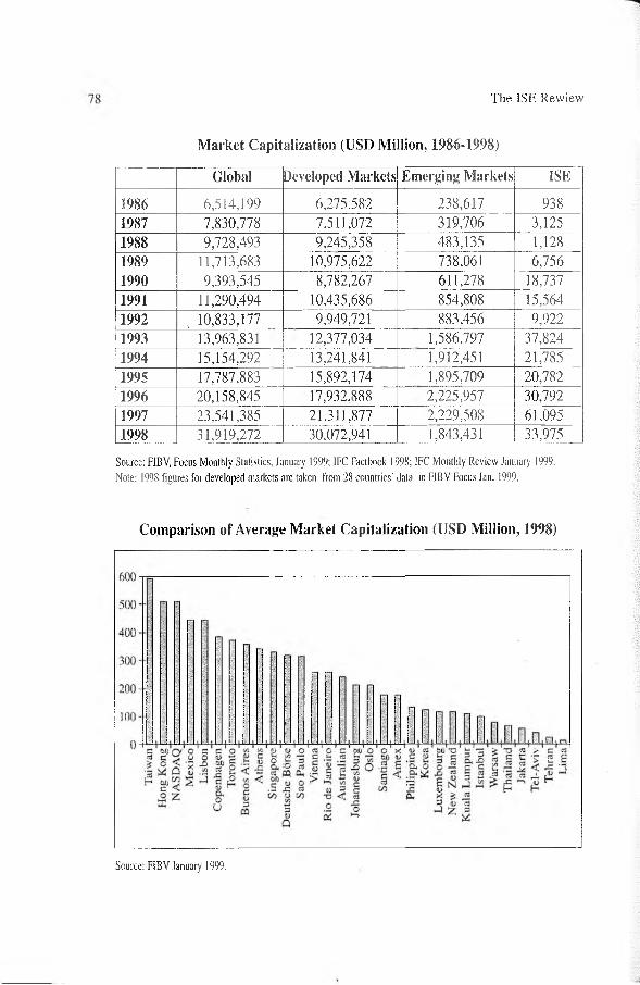
The ISE Rewiew

Market Capitalization (USD Million, 1986-1998)

Global Developed Markets Emerging Markets ISE

1986 6,514,199 6,275,582 238,617 9381987 7,830,778 7,511,072 319,706 3,1251988 9,728,493 9,245,358 483,135 1,1281989 11,713,683 10,975,622 738,061 6,7561990 9,393,545 8,782,267 611,278 18,7371991 11,290,494 10,435,686 854,808 15,5641992 „ 10,833,177 9,949,721 883,456 9,9221993 13,963,831 12,377,034 1,586,797 37,8241994 15,154,292 13,241,841 1,912,451 21,7851995 17,787,883 15,892,174 1,895,709 20,7821996 20,158,845 17,932,888 2,225,957 30,7921997 23,541,385 21,311,877 2,229,508 61,0951998 31,919,272 30,072,941 1,843,431 33,975

Source: FIBV, Focus Monthly Statistics, January 1999; IFC Factbook 1998; 1FC Monthly Review January 1999. Note: 1998 figures for developed markets arc taken from 28 countries' data in FIBV Focus Jan, 1999,

Comparison of Average Market Capitalization (USD Million, 1998)

Source: FIBV January 1999.

Global Capital Markets 79

Worldwide Share of Emerging Capital Markets (19854998)

Source: IFC Factbook 1994-1998, 16-23; IFC Monthly Review, Jan. 1999. F1BV, Focus, Jan. 1999. Note: 1998 global totai data are taken from 50 countries in FiBV, Focus, Jan. 1999.

Share of ISE’s Market Capitalization in World Markets (1986-1998)

3,5%

I I Share in Emerging Markets Share in Developed Markets

Source: IFC Factbooks 1996-1998; IFC M onthly Review, Jan. 1999.

The ISE Rewiew

Main Indicators of Capital Markets 1998

MarketTurnover Velocity (Dec. ‘98}

MarketValue of Share

Trading (million, US$)

Up to Year Total

MarketMarket Cap, of

Shares of Domestic Companies

(millions US$) (Dec.’98)

1 Korea 380,5% NYSE 7.317.949 NYSE 10.271.899,82 NASDAQ 248,0% NASDAQ 5.518.946 NASDAQ 2.524.373,43 Amex 243,3% London 2.887.990 Tokyo 2.439.548,84 Taiwan 224,6% Paris 2.053.300 London 2.297,651,25 Paris 220,3% Deutsche Börse 1,491.796 Osaka 1.871,290,66 Madrid 152,9% Taiwan 895.986 Deutsche Börse 1.094.252,37 Istanbul 120,7% Tokyo 750.831 Paris 985.227,28 Deutsche Borse 113,1% Switzerland 686,956 Switzerland 689,199,39 Athens 97,2% Madrid 640.320 Amsterdam 603.182,2

10 Helsinki 78,9% Italy 488.166 Italy 569.732,111 Switzerland 77,3% Amsterdam 405.211 Toronto 543.394,012 Stockholm 75,1% Toronto 331.848 Montreal 538.533,913 Barcelona 69,5% Chicago 298.912 Madrid 402.162,614 NYSE 68,9% Amex 287.929 Hong Kong 343.566,515 Thailand 65,4% Stockholm 229.961 Bilbao 338.056,016 Italy 64,7% Barcelona 216.159 Barcelona 329.156,817 Oslo 61,4% Hong Kong 206.153 Australian 328.928,518 Lisbon 61,3% Bilbao 200.711 Stockholm 278.707,319 Amsterdam 60,3% Australian 163,054 Taiwan 260.015,120 Singapore 60,1% Osaka 156.567 Brussels 247.583,121 Ljubljana 58,1% Korea 145.061 Johannesburg 168.535,622 Copenhagen 57,1% Sao Paulo 139,583 Rio de Janeiro 162.047,723 Vancouver 56,7% Istanbul 68.479 Sao Paulo 160886,724 Sao Paulo ; 56,2% Copenhagen 64.954 Helsinki 154.832,625 Toronto 52,7% Brussels 61.482 Amex 126.307,026 Bilbao 50,6% Helsinki 61.117 Korea 114.593,327 Australian 47,8% Singapore 58.510 Copenhagen 98.875,628 Warsaw 47,7% Johannesburg 56,941 K.Lumpur 95.561,529 Irish 47,6% Athens 51.393 Singapore 94.986,830 New Zealand 47,3% Lisbon 47.713 Mexico 91.745,831 Tel-Aviv 46,6% Oslo 42.944 Athens 81.552,732 Buenos Aires 42,4% Montreal 37.507 Irish 69.677,033 London 39,3% Irish 36.663 Lisbon 62,954,834 Hong Kong 32,1% Rio de Janerio 33.279 Santiago 51.866,235 Phillippine 30,7% Mexico 31.192 Oslo 46.420,936 Vienna 30,1% Kuala Lumpur 26.839 Buenos Aires 45.332,337 Jakarta 30,0% Buenos Aires 26.056 Tel-Aviv 40.883,438 Tokyo 28,9% Thailand 20.976 Luxembourg 38.138,539 Lima 27,3% Vienna 17.384 Vienna 35.778,940 Brussels 27,0% Tei-Aviv 15.079 Philippine 35.297,041 Johannesburg 23,8% New Zealand 14.279 Thailand 34.252,442 Mexico 21,0% Jakarta 10.637 Istanbul 33.645,643 K. Lumpur 16,8% Philippine 10.148 New Zealand 24.784,044 Tehran 15,9% Warsaw 8.913 Jakarta 22.077,945 Rio de Janerio 9,4% Santiago 4.411 Warsaw 20.461,146 Osaka 8,1% Lima 3.050 Tehran 14.903,347 Montreal 6,0% Vancouver 2.574 Lima 9.868,548 Santiago 5,0% Luxembourg 1.561 Vancouver 4.482,049 Luxembourg 4,1% Tehran 1.362 Ljubljana 2.984,9

Source: FIBV, Focus. Jan. 1999.

G lobal Capital M arkets 81

Trading Volume (USD millions, 1986-1998)

Global Developed Emerging ISE Emerging/Global

(%)

ISE / Emerging

(%)1986 3,573,570 3,490,718 82,852 13 2.32 0.021987 5,846,864 5,682,143 164,721 118 2.82 0.071988 5,997,321 5,588,694 408,627 115 6.81 0.021989 7,468,215 6,302,687 1,165,528 773 15.61 0.071990 5,512,129 4,617,688 894,441 5,854 16.23 0.651991 5,016,379 4,410,855 605,524 8,502 12.07 1.421992 4,778,429 4,165,501 612,928 8,567 12.83 1.341993 7,702,502 6,633,684 1,068,818 21,770 13.88 2.1719 94 10,085,703 8,445,585 1,640,118 23,203 16.26 1.321995 11,666,260 10,632,763 1,033,497 52,357 8.86 4.971996 13,580,050 11,993,232 1,586,818 37,737 11.7 2.381997 19,484,706 16,782,995 2,701,711 58,104 13.9 2.151998 26,854,776 24,887,784 1,966,992 70,396 7.33 3.58

Source: IFC Factbooks 1997-1998; FIBV Focus Jan. 1999.Note: 1998 figures for developed markets are taken from 28 countries in F1BV Focus Jan. 1999.

Number of Trading Companies (1986-1998)

Global Developed Emerging ISE Emerging/Global

(%)

ISE / Emerging

(%)1986 28,173 18,555 9,618 40 34.14 0.421987 29,278 18,265 11,013 50 37.62 0.451988 29,270 17,805 11,465 50 39.17 0.441989 29,486 17,478 12,008 50 40.72 0.421990 28,918 16,403 12,515 110 43.28 0.881991 25,951 16,315 9,636 134 37.13 1.391992 27,586 17,227 10,359 145 37.55 1.401993 28,768 17,431 11,337 152 39.41 1.341994 36,078 19,064 17,014 176 47.16 1.031995 38,864 19,467 19,397 205 49.91 1.061996 42,351 20,088 22,263 228 52.60 1.361997 40,593 '20,656 19,937 258 49.1 1.291998 38,944 21,781 17,163 277 44.1 1.61

Source: IFC Factbooks 1997-1998; FIBV Focus Jan. 1999.Note; 1998 figures for developed markets are taken from 28 countries in FIBV Focus Jan. 1999.

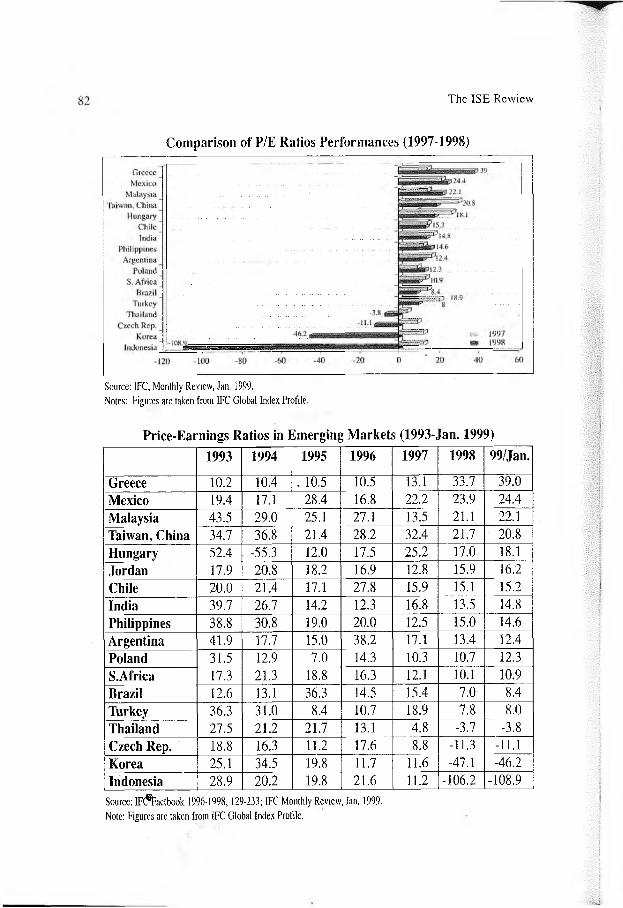
The ISE Rewiew

Comparison of P/E Ratios Performances (1997-1998)

Source: IFC, Monthly Review, Jan. 1999.Notes: Figures arc taken from IFC Global Index Profile.

Price-Earnings Ratios in Emerging Markets (1993-Jan. 1999)

1993 1994 1995 1996 1997 1998 99/Jan.

Greece 10.2 10.4 . 10.5 10.5 13.1 33.7 39.0Mexico 19.4 17.1 28.4 16.8 22.2 23.9 24.4Malaysia 43.5 29.0 25.1 27.1 13.5 21.1 22.1Taiwan, China 34.7 36.8 21.4 28.2 32.4 21.7 20.8Hungary 52.4 -55.3 12.0 17.5 25.2 17.0 18.1Jordan 17.9 20.8 18.2 16.9 12.8 15.9 16.2Chile 20.0 21.4 17.1 27,8 15,9 15.1 15.2India 39.7 26.7 14.2 12.3 16.8 13.5 14.8Philippines 38.8 30.8 19.0 20.0 12.5 15.0 14.6Argentina 41.9 17.7 15.0 38.2 17.1 13.4 12,4Poland 31.5 12.9 7.0 14.3 10.3 10.7 12.3S.Africa 17.3 21.3 18.8 16.3 12.1 ,10.1 10.9Brazil 12.6 13.1 36.3 14.5 15.4 7.0 8.4Turkey 36.3 31.0 8.4 10.7 18.9 7.8 8.0Thailand 27.5 21.2 21.7 13.1 4.8 -3.7 -3.8Czech Rep. 18.8 16.3 11.2 17.6 8.8 -11.3 -11.1Korea 25.1 34.5 19.8 11.7 11.6 -47.1 -46.2Indonesia 28.9 20.2 19.8 21.6 11.2 -106.2 -108.9

Source: IF(?Factbook 1996-1998,129-233; IFC Monthly Review, Jan. 1999. Note: Figures are taken from IFC Global Index Profile.

G lobal Capilal M arkets 8 3

Comparison of Market Returns In USD (1998- Jan. 1999)S. korea _________ ■ ______________________ i____■______ 14,-iGreece ■■ ■ ■ ......... : ............■■■..... r n

Thailand .... ..............■■■T14SPhilippines j t) Ï

Malaysia 3 2.4Singapore -1.7 Ë

China -2 .9 mHong Kong -4.2 Iœ

Poland E S Q

Czech Rep. - 1 1 .6 E S I

Israel - U .8India - 1 6 .5 l

Egypt -14.7 1....... -Taiwan -il J 1. a.

HungaryS. Africa -2K.il-....... ■

Indonesia - n i ! ■■■....■■■-.Chile s r — ......

Colombia •n > i — ---------Argentina •*S.21..................

Mexico -S I * : ........ .............Brazil

Turkey -, i ■ :------------- -- . .Venezuela .•>. .1 .................

Russia ■<.. • ! .......- .... ..... -r — i ...-120 -80 -40 0 40 SO 120 160

Source: The Economist

Market Value/Book Value Ratios (1993-Jan. 1999)

1993 1994 1995 1996 1997 1998 99/Jan.Greece 1.9 1.9 1.8 2.0 2.9 4,9 5,6H ungary 1.6 1.7 1.2 2.0 3.7 3,2 3,4Taiwan, China 3.9 4.4 2.7 3.3 3.8 2,7 2,7Turkey 7.2 6.3 2.7 4.0 9.2 2,6 2,5Jordan 2.0 1.7 1.9 1.7 1.6 1,9 2,0India 4.9 4.2 2.3 2.1 2.7 1,8 1,8S.Africa 1.8 2.6 2.5 .2.3 1.9 1,5 1,8Mexico 2.6 2.2 1.7 1.7 2.5 1,5 1,7Poland 5.7 2.3 1.3 2.6 1.6 1,6 1,6Argentina 1.9 1.4 1.3 1.6 1.8 1,4 1,4Philippines 5.2 4.5 3.2 3.1 1.7 1,3 1,4Chile 2.1 2.5 2.1 1.6 1.6 1,3 1,2Thailand 4.7 3.7 3.3 1.8 0.8 1,3 1,2Indonesia 3.1 2.4 2.3 2.7 1.5 1,2 1,2Malaysia 5.4 3.8 3.3 3.8 1.8 1,1 1,1Czech Rep. 1.3 1.0 0.9 0.9 0.8 0,9 1,0Brazil 0.5 0.6 0.5 0.7 1.1 0,7 0,7Korea 1.4 1.6 1.3 0.8 0.6 0,6 0,7

Source: IFC Faclbook 1996-1998, pp. 129-233; IFC Monthly Review, Jan. 1999.

8 4 The ISE Rewiew

Market Value of Bonds (Million USD, Jan.-Dee. 1998)

Paris Italy

London

Stockholm

Johannesburg Deutsche Börse

Copenhagen Amsterdam

Switzerland Oslo

Santiago

Bilbao Barcelona

Tokyo Istanbul

Amex

IrishBuenos Aires

Tel-Aviv Lisbon

Korea

Brussels Osaka

NYSE Madrid

Lima Luxemburg

Taiwan Warshaw

Mexico

Singapore Vienna

Athens Kuala Lumpur

Australian

Ljubljana New Zealand

Helsinki Montreal

NASDAQ

t - v vH 13.656.087,6 2.710.927,5

11.813.326,2 1.640.838,5 1.503.869,8 1.498.924,7

11.300.065,8296.234,0

159.349,51148.175,3

96.371,289.805.574.414.5

68.219,9 66.525,0 65.594,2

48.568.635.634.7

18.850,3J 18.271,9

111.394,94.848,5

4.408.2 3.835,52.104.2

1.919,11.462,31.241.21.224.3

941,5 885,8

470,43433,9

141.3139.3

1135,5128.3

........... ........ 170Q

I100

: !---- 1-1.000 10.000

---- !---- J ,100.000 1.000.000 10.000.000 100.000.000

Source: FIBV, Focus, Monthly Statistics, Jan. 1999.

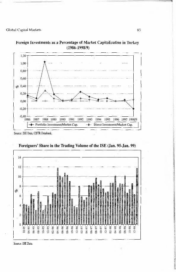
G lobal Capital M arkets 85

Foreign Investments as a Percentage of Market Capitalization in TYirkey(1986-1998/9)

Source: ISE Data.

The ISE Rewiew

0,55

Price Correlations of the ISE (Jan. 1994-Jan. 1999)

0,50

0,45

0,40

0,35

0,30-

0,25

0,20

0,15

0,10

0,05

0,00

-0,05

Czech Rer

FT-100

Iordan

Lidia

• Indonesia

»Philippines

K orea......0 I©Thailand

NikJcei

©M alaysia ©China ► Taiwan

•R u ssia

Hungary®

IFCI Composi te *• Greece

Chile •B raz ilS&P.500 »M exico

• Argentina

a S.A frica

Notes: The correlation coefficient is between 4 and +1. If it is zero, for the given period, it is implied that there is no relation between two series of returns. For monthly return index correlations (IFCI) see. IFC, Monthly Review, Jan. 1999

Comparison of Market Indices (Jan 97=100)

Source: Reuters.Note: Comparisons are in USD.

The ISE Review Volume: 3 No: 9 January/Febmary/March 1999ISSN 1301-1642 © ISE 1997

ISEMarket Indicators

STOCK MARKET

Total Value Market Value DividendYield

P/ERatios

Î '1 Toial Daily Averagei s

c3 (TL Billion) (US$ Million) (TL Billion) (US$ Million) (TL Billion) (US$ Million) «198 6 80 9 13 — 709 938 9.15 5.07

198 7 82 105 118 — — 3,182 3,125 2.82 15.86

i98 8 7 149 115 1 — 2,048 1,128 10.48 4.97

198 9 76 1,736 773 7 3 15,553 6,756 3.44 15.74

199 0 no 15,313 5,854 62 24 55,238 8,737 2,62 23.97

199 1 134 35,487 8,502 144 34 78,907 15,564 3.95 15.88

1992 145 56,339 8,567 224 34 84,809 9,922 6.43 11.39

1993 160 255,222 21,770 1,037 89 546,316 37,824 1.65 25.75

199 4 176 650,864 23,203 2,573 92 ■ 836,118 21,785 2.78 24.83

199 5 205 2,374,055 . 52,357 9,458 209 1,264,998 20,782 3,56 9.23

199 6 228 3,031,185 37,737 12,272 Î53 3,275,038 30,797 2.87 12.15

1997 258 9,048,721 58,104 35,908 231 12,654,308 61,879 1.56 24.39

1998 277 18,029,967 70,396 72,701 284 10,611,820 33,975 3.37 8.84

1999/QIC) 278 2,982,403 8,925 85,212 255 15,752,332 45,034 2.44 11.48

(■) The first quarter includes the Januaiy-Februaiy period.

The ISE Review

Closing Values of the ISE Price Indices

TL BasedNATIONAL-lOO (Jan. 1986=1)

NATI0NAL-1NDÜSTRIALS (Dec.31,90=33)

NAT10NAL-SERVICES (Dec.27,96=i046)i

NATIONAL-FINANCIAL') (Dec. 31,90=33)

1986 1.71 — — —

1987 6.73 — — —

1988 3.74 — — —

1989 22.18 — — —

1990 32.56 32.56 t 32.56 •

19 91 43.69 49.63 — 33.55

1992 40.04 49.15 — 24.34

1993 206.83 222.88 191.901994 272.57 304.74 229.64

1995 400.25 462.47 — 300.04

1996 975.89 1,045:91 1,045.91 914.47

1997 3,451.26 2,660.00 3,593.00 4,522.00

1998 2,597.91 1,943.67 3,697.10 3,269.58

1999/Q10 3,890.83 2,571.63■ ■■■■ ■■ TTC <£• 1>

5,282.76 5,099.84

NATIÛNAL-100 (Jan. 1986=100)

US $ UNATI0NAL-1NDUSTR1ALS

(Dec.31,90=643)

asedNATIONAL-SERVICBS

(Dec.27,96-572)NAÏÏ0NAL-FINANCIALS

(Dec. 31,90=643)1986 131.53 — —

1987 384.57 — — ■ —

1988 119.82

1989 560.57 — — —

1990 642.63 : : 642.63

1991 501.50 569.63 385.14

1992 272.61 334.59 ----' 165.68

1993 833.28 897.96 -- 773.13

1994 413.27 462.03 — 348.18

1995 382.62 442.11 - 286.83

1996 534.01 572.33 572.— : 500.40

1997 981.99 756.91 1,022.40 1,286.75

1998 484.01 362.12 688.79 609.14

1999/Qlf) 647.28 427.82 878.84 848.41

C): The first quarter figures are as of February 26,1999.

İSE M arket Indicators 89

BONOS AND BILLS MARKET

Traded Value

Outright Purchases and Sales Market

Total Daily AverageTL Billion US$ Million TL Billion US$ Million

1991 1,476 312 11 2

1992 17,977 2,406 72 10

1993 122,858 10,728 499 44

1994 269,992 8,832 1,067 35

İ995 739,942 16,509 2,936 66

1996 2,710,973 32,737 10,758 130

1997 5,503,632 35,472 21,840 141

1998 17,995,993 68,399 71,984 274

1999/OH*) 4,031,872 12,157 108,970 329

Repo-Reverse Repo Market

Total Daily AverageTL Billion US $ Million TL Billion US $ Million

1993 59,009 4,794 276 22

1994 756,683 23,704 2,991 94

1995 5,781,776 123,254 22,944 489

1996 18,340,459 221,405 72,780 879

1997 58,192,071 374,384 230,921 1,485

1998 97,278,476 372,201 389,114 1,489

1999/Q10 21,936,731 66,043 592,885 1,785

(*): The first quarter includes the Jamıary-Febıuary period.

90 The ISE Review

— IS E G D S P r i c e Indices (D ecem ber 25-29, 1995=100)

TL Based

30 Days 91 Days 182 J)ays General1996 103.41 110.73 121,71 110.52

1997 102.68 108,76 118.48 110.77

1998 103.57 110.54 119.64 110.26

1999/Q10 104.02 112.29 123.95' 115.09

— ISE GDS Performans Indices (December 25-29,1995=100)

I TL Based

30 Days 91 Days 182 Days1996 222.52 240.92 262.20

1997 441.25 474,75 525.17

1998 812.81 897.19 983.16

1999/Q10 904.19 1,007.18 1,137.52

US $ Based

1996 122.84 132.99 144.74

1997 127.67 137.36 151.95

1998 153.97 169.96 186.24

1999/Q10 152,95 170.37 192.41

(*}: The first quarter figures are as of February 2 6 ,1999.

The ISE Review Volume: 3 No: 9 January/February/March 1999ISSN 1301-1642 © ISE 1997

Book Reviews

Emerging Markets: Research, Sfrategies and Benchmarks, Michael Keppler and Martin Lechner, McGraw-Hill, 1997, pp. x + 374.

Institutional investors who anticipate high returns for their investments and wish to diversify their portfolio, are increasingly directing their attention towards the emerging markets. When low correlations between these markets, both among each other and with developed markets, are combined with high returns, an unconceivable opportunity arises in the diversification of investment portfolios. From the middle of 1980’s, these advantages of the emerging markets, have been better understood by international investors and in line with this fact, a rapid increase was observed in the trading volumes, market capitalization and number of listed companies of the emerging markets. In addition to the great potential presented by the emerging markets, the investors who invest in these markets are face to face with a high risk.

The book named “the emerging markets” considers the potential of emerging markets provided, in particular, for the foreign investors and the risks that could be faced by these investors, and suggests suitable investment strategies. With this aim, the book consists of five? main parts including an introduction and an appendix. Michael Keppler who is one of the writers of the book is the manager of an investment consultancy firm named “Keppler Wealth Managing” that provides consultancy services to an investment fund which won the best performer prize in the category of emerging markets in the years between 1994 and 1995. Martin Leachner who is also the writer of the book have worked in several financial firms in different countries and currently, he works as a market expert in the emerging bond market at an international investment bank.

Following the introduction part, the second part named “the emerging markets and international capital markets” defines the emerging markets concept and provides information on the characteristics of such markets and their differences from developed markets in terms of benchmark indicators such as market capitalization, trading volume and number of listed firms. Following these, the reasons for the high growth rate which is considered the main characteristics of the emerging markets, in com

The ISE Review

parison with developed markets, are analyzed on the basis of countries and regions and forecasts are made for the future. The section continues with the high potential in the emerging markets, possible political and economical risks that may be faced by investors in these markets, their reasons and the adversities that prevailed in the years 1994 and 1995 are examined in depth. At the end of the part, correlations among various emerging markets and the risk/return profiles are analyzed and compared with the developed markets. Emerging markets’ major composite indices that are useful indicators in the decision making process for international investors are also mentioned in this section.

In the third part named “investment strategies”, the selected investment strategies are defined and analyzed according to potential risk and returns. As a result of comparisons made with the Morgan Stanley Capital International (MSCI) World Index which is a market capitalization Index that consists of developed markets show that equally weighted emerging markets give better results. Smaller markets that have low market capitalization provide higher return and lower risk. As a result, the investment strategies that work in developed markets can also be transferred to the emerging markets.

The fourth part is called the “assignment of the wealth”. In this part, the methods that are used by the investor in the most appropriate way for the assignment of different wealth groups like stock certificates representing investment capital, public sector bonds and money market instruments according to the investment period and level of risk-taking are taught. Assignment of wealth is made by comparing the IFCI Compound Index and S & P 500 index with the emerging markets in years between 1989-1995. The same process is realized by the comparison of the IFCI Compound Index and MSCI World Index among the emerging and developed markets. Thus, we can calculate the portion of the portfolios that can be assigned to the emerging markets, for those investors who wish to minimize their risk or to attain the highest return free from risk.

In the fifth part, the investment opportunities and ways that the investors in developed countries have seen in emerging markets are examined. The difficulties that may be faced by the investors who invest directly in emerging markets are stated while investing in depositary certificates representing stock certificates in developed markets was mentioned as a second alternative to invest in emerging markets. As a third method, the advantages and disadvantages of investing in open-ended and close-ended stock certificate investment funds in the emerging markets are explained.

Book Reviews 93

Another method mentioned in the section is buying/selling options issued in the emerging markets or the futures and options markets based on indices in these markets. Finally, buying/selling stock certificates of companies that are listed in the developed markets and which have a business concern in the emerging markets was also stated as another option of investing in emerging markets.

In the appendix part, each one of the 25 emerging stock markets that are comprised in the IFCI Index of the International Finance Corporation are analyzed in terms of agriculture, industry, trade, the development of the economy and stock markets and effective regulations that concerns foreign investors.

“Financial E n g i n e e r i n g A Complete Guide to Financial Innovation. Jack F. Marshall & Vipul Bansal, New York Institute of Finance, 1992, xxiv+728.

The book entitled “Financial Engineering”: A Complete Guide to Financial Innovation which is written by two well-known authors Jack F. Marshall and Vipul Bansal, is a New York Institute of Finance press in 1992.

Consisting of five main parts that concentrate on financial engineering, the book combines the theoretical and practical systematics with an original style and handles almost all aspects of the subject in a way to satisfy the needs of all-level-readers.

The first section is a guide for those who deals with the subject and wish to have a carrier in the field and consists of the definition and concept of financial engineering, the tools of this discipline, the fields in which the financial engineering is widely used and a comparison of financial engineering and financial analysis. The section also provides information on the environmental factors such as: price volatility, globalization of the markets, tax asymmetries, technological advances, advances in financial theory, changes in regulations, decreases in transactions and information costs as a result of the increasing competition. Moreover, the part sheds light on the intrafirm factors such as: liquidity, risk aversion, agency costs and accounting benefits, which the firms need.

The first subtitle of the second section titled “Valuation Relationships and Applications” mainly focuses on: the cash flows, time

94 The ISE Review

value and sensitivity of time value. The following two chapters of this section provides theoretical information on measuring return, portfolio consideration, investment horizon, mathematics of portfolio analysis while chapter seven moves one step further and introduces advanced techniques for risk measurement and hedging tools, measuring hedge effectiveness and finally the cost of hedging. Debt instruments and their valuations, the yield curve, risk inherent in investments such as interest rate risk, default risk, reinvestment risk, call risk, prepayment risk, purchasing power risk are all discussed in chapter eight, entitled “Understanding Interest Rates and Exchange Rates”. The chapter also focuses on the determinants of exchange rate and comparative yield curves. Speculation, arbitrage and market efficiency, the corporate treasurer’s perspective, the importance of risk management are the other subjects of the rest of the chapters of the second section.

The third section in which the physical tools of financial engineering are introduced, consists of nine parts of which the first three deals with product development, futures and forwards and swaps. The fourteenth chapter goes into detail on single period options, calls and puts, multiperiod options: caps, floors, collars, captions, swaption and compound options. Fixed income securities, recent debt market innovations, equity and equity-related instruments, hybrid securities are also discussed in detail in the last three chapters of section three.

In section four, namely the “Financial Engineering Processes and Strategies” constitutes the following subjects: assets liability management, hedging and related risk management techniques, corporate restructuring and the LBO, arbitrage and synthetic instruments, tax driven deals and miscellaneous equity-based strategies.

The book in which almost all of the subjects of financial engineering are examined in detail, ends with a section in which the future directions of financial engineering, the effects of globalization and technology on future trends, legal protections for innovative financial products and services are discussed.

The book is written in a simple and easy to understand manner and it is not only intended for the experts within this field but also the ones who are not very familiar with the subject. With its success in providing the logic of financial engineering beyond all those complex and complicated mathematical formulations, the book is an excellent source for those dealing with the subject and those already working in the field.

Book Reviews 95

Investment Intelligence from Insider Trading, H. Nejat Seyhun, The MIT Press, 1998, pp. xxxvii + 402.

Insider trading can be defined as legal stock transactions of the officers, directors, and large shareholders of a firm in order to make significant profits, using the information which is about the firm’s realities that has been attained earlier than the public. Therefore, outsiders may well consider that imitating publicly available insider trading could provide higher gains than using other information. Given the extra costs and risks of an active trading strategy, the key question for stock market investors is whether publicly available insider trading information can help them to outperform a simple passive index fund.

In the book which has been written by H. Nejat Seyhun, by using the reported insider trading of all publicly held firms over a period of twenty- one year data base (over one million transactions), it has been shown how the investors can use insider information to their advantage. Moreover, the book analyzes the magnitude and duration of the stock price movements, insiders’ profits and risks associated with imitating insider trading after an insider trading has been realized. He also overviews the likely performance of individual firms and of the overall stock market, and compares the value predicted by insider trading with the value of commonly used indicators such as price-eamings ratio, book-to-market ratio, and dividend yield. The goal of the book is to determine whether the outsiders’ portfolio performances significantly increase through using the reported insider trading information.

The book contains three main parts comprised of fifteen chapters including an introduction. In the first section that includes introduction and the first five chapters, the prediction ability of insider trading variables is analyzed. Within the second section from chapter six to thirteen, prediction ability of insider trading of a share value is compared with the commonly-used variables. Cahpter fourteen which is the last part of the book, an implementation strategy is defined and some recommendations are presented to outsider investors.

In the introduction chapter, after insider trading is defined and some background information is provided, the regulations about insider trading are presented. Moreover, the generally-used investment strategies of investors are reviewed and the usefulness of the book to the outsiders is explained.

The ISE Review

After the first chapter that explains the database and variables used in various analysis, the second chapter focuses on how reported insider trading database can be utilized to predict future price movements of stocks. Chapter Three is related to be establishment of stock selection strategies by using the insider trading database. Following the third chapter in which specific stock returns are analyzed, future movements of stock markets, in general, are examined in the fourth chapter. This subject especially is important for determining the market timing. The following chapter provides a method that predict the 1987 market crash.

The first chapter of second part -Chapter Six- compares insider trading with dividend yield to predict the future price movements of stocks. In the following chapter dividend announcement and insider trading are compared. Chapter eight examines comparatively whether insider trading can be used to improve the earnings drift strategies prior to profit announcements that differ from outsiders’ expectations. Chapters Nine and Ten examine the predictive ability of price-eamings ratio (P/E) and book-to-market ratio (B/M) used to determine the fair price of a stock and introduce insider trading as another forecasting variable that can affect the predictive ability of the P/E ratio and the B/M ratio. Chapters eleven and twelve look at corporate takeovers and insider trading around corporate takeovers. They examine whether it is possible to predict the takeover status of bidder and target firms using pre-announcement insider trading. Thirteenth chapter examines the performance of momentum and mean- reversion investment strategies and whether insider trading can be used to improve these strategies. In this chapter the predictable patterns in stock returns using past winners and losers are examined. It is also examined insiders’ reaction to large stock price movements in the past to determine if insiders view these price changes as a potential profit opportunity.

Last part of the book -fourteenth chapter- examines the availability of profits to outsiders who mimic insiders’ transactions. Outsiders interested in mimicking insider trading have to deal with three additional concerns: reporting delays, transaction costs, and the risk of incurring losses from imitating a small number of transactions. The objective of the chap

iter is to take a realistic approach by replicating the information available to outsiders and including the trading costs. The chapter concludes with recommendations to outside investors.

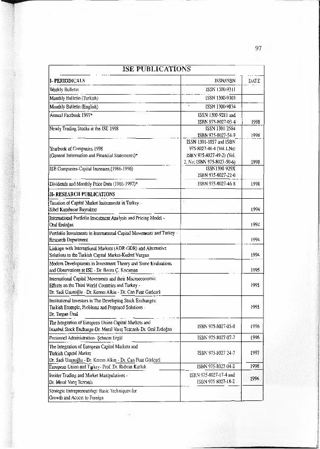
ISE p u b l i c a t i o n s

I- PERIODICALS ISSN/ISBN DATEWeekly Bulletin ISSN 1300-9311Monthly Bulletin (Turkish) ISSN 1300-9303Monthly Bulletin (English) ISSN 1300-9834Annual Factbook 1997* ISSN 1300-928 i and

ISBN 975-8027-03-4 1998Newly Trading Stocks at the ISE 1998 ISSN 1301-2584

ISBN 975-8027-54-9 1998

Yearbook of Companies 1998(General Information and Financial Statements)*

ISSN 1301-1057 and ISBN 975-802748-4 (Vol.LNo*

ISBN 975-802749-2) (Vol. 2. No: ISBN 975-8027-50-6) 1998

ISE Companies-Capital Increases,(1986-1996) ISSN 1300-929X ISBN 975-8027-22-0

Dividends and Monthly Price Data (1986-1997)* ISBN 975-802746-8 1998

II- RESEARCH PUBLICATIONSTaxation of Capital Market Instruments in Turkey - Sibei Kumbasar Bayraktar 1994International Portfolio Investment Analysis and Pricing Model - Oral Erdoğan 1994Portfolio Investments in Internationa! Capital Movements and Turkey - Research Department 1994Linkage with International Markets (ADR-GDR) and Alternative Solutions to the Turkish Capital Market-Kudret Vurgun 1994Modern Developments in Investment Theory and Some Evaluations and Observations at ISE - Dr, Berna Ç. Kocaman 1995International Capital Movements and their MacroeconomicEffects on the Third World Countries and Turkey -Dr. Sadi Uzunoğlu - Dr. Kerem Alkin - Dr. Can Fuat Gürleşe!

1995

Institutional Investors in The Developing Stock Exchanges: Turkish Example, Problems and Proposed Solutions - Dr. Targan Ünal

1995

The Integration o f European Union Capital Markets and Istanbul Stock Exchange-Dr. Meral Varış Tezcanh-Dr. Oral Erdoğan ISBN 975-8027-05-0 1996

Personnel Administration- Şebnem Ergül ISBN 975-8027-07-7 1996The Integration o f European Capital Markets and Turkish Capita! Market -Dr. Sadi Uzunoğlu - Dr. Kerem Alkin - Dr. Can Fuat Giirlesel

ISBN 975-8027-24-7 1997

European Union and T ykey- Prof. Dr. Rıdvan Karluk ISBN 975-8027-04-2. 1996Insider Trading and Market Manipulations - Dr. Meral Varış Tezcanlı

ISBN 975-8027-17-4 and ISBN 975-8027-18-2 1996

Strategic Entrepreneurship: Basic Techniques for Growth and Access to Foreign

98

I S E p u b l i c a t i o n sMarkets for Turkish Companies-Omer Esener ISBN 975-8027-28-X 1997

Research Studies on Capital Markets and ISERegulations Related to Capital Market Operations- Vural GünaS

ISBN 975-7869-04-X ISBN 975-8027-34-4

19961997

Resolution of Small and Medium Size Enterprises’ Financial Needs Through Capital Marketi - R, Ali Küçükçolak ISBN 975-8027-39-5 1998

Equity Options and Trading on the ISE - Dr. Mustafa Kemal Yılmaz ISBN 975-8027-45-X 1998Private Pension Funds : Chilean Example - Çağatay Ergenekon ISBN 975-8027-43-3 1998Analysis of Return Volatility In the Context o f Macroeconomic Conjuncture - Prof. Dr. Hurşit Güneş- Dr. Burak Saltoglu ISBN 975-8027-32-8 1998

What Type of Monetary System? Monetary Discipline and Alternative Resolutions for Monetary Stability - Prof. Dr. Coşkun Can Aktan - Dr. Utku Utkulu-Dr. Selahattin Togay

ISBN 975-8027-47-6 1998

Institutional Investors in the Capital Markets (Dr. Oral Erdoğan-Levent Özer) ISBN 975-8027-51-4 1998Repo and reverse Repo Transactions - Dr. Nuran Cömert Doyrangöl ISBN 975-8027-12-3 1996South Asian Crisis: The Effects on Turkish Economy and the ISE - Research Department ISBN 975-8027-44-1 1998

RESEARCH ON DERIVATIVES MARKETSome Basic Strategies on Securities Market derived from Future Transactions and Options (Mustafa Kemal Yılmaz) 1996

SECTORAL RESEARCHAutomotive Sector- Sibel Kumbasar Bayraktar 1995Textile Sector (Cotton)- Efser Uytun 1995Food Sector - Ebru Tan 1995Glass Sector- Özlem Özdemir 1995Insurance Sector- Çağatay Ergenekon 1995Tourism Sector- Oral Erdoğan 1995Manifactural Paper and Paper Product Sector- Çağatay Ergenekon ISBN 975-8027-09-3 1996Textile Sector (Artificial-synthetic. Woolen. Manufactured Clothing, Leather and Leather Goods)- Efser Uytun ISBN 975-8027-10-7 1996

Food Sector (Vegetable Oil, Meat, Fruit. Dairy Products, Sugar, Flavor Products, Animal Feed) Research Department ISBN 975-8027-19-0 1997

EDUCATIONBasic Information Guide on Capital Markets and Stock Exchange (May 1998) ISBN 975-8027-41-7 1998

III- BOOKLETSQuestions-Answers: ISE and Capital Markets ISBN 975-8027-31-X 1997Guide on Stock Market Transactions ISBN 975-8027-35-2 1997Investors Counselling Center(*) Publications marked by (*) are in Turkish and English.For further inquiries please contact :Training and Publications DepartmentTel : 90 (0212) 298 24 24Fax : 90 (0212) 298 25 00

O bjectives and CoutenfsThe ISE R eview is a journal published quarterly by the Istanbul Stock Exchange (ISE). Theoretical and empirical articles examining primarily the capital markets and securities exchanges as well as economics, money, banking and other financial subjects constitute the scope o f this Journal. The ISE and global securities market performances and book reviews will also be featuring, on merits, within the coverage of this publication.

Copy Guides for AuthorsArticles sent to the ISE R eview will be published alter the examination o l the Managing Editor and the subsequent approval o f the Editorial Board, Standard conditions that the articles should m eet for publication are as follows;1. Articles should be written in both English and Turkish.2. Manuscripts should be typed, single space on an A 4 paper (210 mm. x 297 mm.) with at least 3 cm. margins. Three (3) copies

of the texts should be submitted to:Istanbul Menkul Kıymetler Borsası (ISE),Araştırma Bölüm ü (Research Department)Istinye, 80860, Istanbul T U R K E YArticles will not be returned to the authors. The ISE is not responsible for lost copy or late delivery due to complications during the mailing process.

3. Articles should be original, unpublished or shall not be under consideration for publication elsewhere.4. If and when the article is approved by the Editorial Board, the author should agree that the copyright for articles is

transferred to the publisher. The copyright covers the exclusive right to reproduce and distribute the articles.5. If necessary, the Editorial Board may demand changes, deletions and/or modifications in the contents of the article without

infringing on the basic structure o f the text,6. Articles, approved for publication, should be written in Windows, Word and Excel programs for PC and should be despatched

to the address above, formatted in a 3.5-inch disk.7. The first page of the article should contain a concise and informative title, the full name(s) and afflliation(s) o f the author(s)

and an abstract o f not m ore than 1(H) words, summarizing the significant points o f the article. The full mailing address, telephone and fax numbers o f the corresponding author, acknowledgements and other related notes should also appear in the first page as footnote(s).

8. The main text should be arranged in sequentially numbered sections. The first scction should be titled “Introduction,” while the last section should be titled “Conclusion” as the others should be titled and numbered with a second digit (2 .1 ,3 .2 and so on). Using boldface is necessary to indicate headings,

9. References to personalities in the text should be entered as: Smith (1971) or ( Smith, 1971); two a u th o rs: Smith and Mill (1965) or (Smith and Mill, 1965); three or more authors: Smith, et al. (1974) or (Smith et al., 1974). References to papers by the sam e author(s) in the sam e year are distinguished by the letters a, b, c, etc. (e.g. Smith, 1974a). References should be listed at the end o f the paper in alphabetical order.

10. Footnotes should be subsequently numbered and are to be placed at the bottom o f the related page. Examples o f footnote use are:-Books with one author:

'Hormats, Robert D ., “Reforming the International Monetary System; From Roosevelt to Reagan," Foreign Policy Association, N ew York, 1987, pp. 21-25.

-Books with two authors:'H oel, P.G., Port, S.C. "Introduction to Probability Theory, ” H oughton Mifflin Company,U S, 1971, p. 241.

-Books with more than three authors:^Mendenhall, W,, et al., "Statistics for Management and Economics,” Sixth Edition, WPS K ent Publishing Company, Boston, 1989, p, 54,

-Articles:'Harvey, Campbell R., "The World Price o f Covariance Risk," The Journal o f Finance,Vol. XLVI, N o .l, March 1991, pp. 11-157.

-Publications on behalf o f an institution:'Federal Reserve Bulletin, Washington, 19924993-1994.

11. Tables and figures should be sequentially numbered with a brief informative title. They should be com prehensible without reference to the text incorporating the full text, heading and unit o f measurements. Source o f the information and explanatory footnotes should be provided beneath the table or figure.

12. Equations should be centered and displayed on a separate line. They should be numbered and referred to in the main text by their corresponding numbers. D evelopm ent of mathematical expressions should be presented in appendices,

Documents

Osman Karamusfafa Ala Murutoglu Alper OzuimOsman Karamusfafa Leading Indicators Approach for Business Cycle Forecasting and a Study ... M urad KAYACAN Gürsel KONA Dr. M. Kemal YILM