OS Fall’02

Performance Evaluation

Operating Systems Fall 2002

OS Fall’02

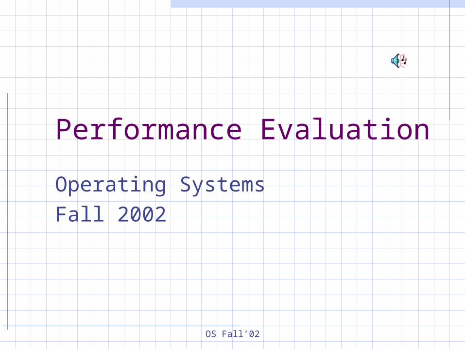
Performance evaluation There are several approaches for

implementing the same OS functionality

Different scheduling algorithmsDifferent memory management schemes

Performance evaluation deals with the question how to compare wellness of different approaches

Metrics, methods for evaluating metrics

OS Fall’02

Performance Metrics

Is something wrong with the following statement:

The complexity of my OS is O(n)?

This statement is inherently flawedThe reason: OS is a reactive program

What is the performance metric for the sorting algorithms?

OS Fall’02

Performance metrics Response time Throughput Utilization Other metrics:

Mean Time Between Failures (MTBF)Supportable load

OS Fall’02

Response time The time interval between a user’s

request and the system responseResponse time, reaction time, turnaround time, etc.

Small response time is good:For the user: waiting lessFor the system: free to do other things

OS Fall’02

Throughput Number of work units done per time

unitApplications being run, files transferred, etc.

High throughput is goodFor the system: was able to serve many clientsFor the user: might imply worse service

OS Fall’02

Utilization Percentage of time the system is

busy servicing clientsImportant for expensive shared systemLess important (if at all) for single user systems, for real time

systems

Utilization and response time are interrelated

Very high utilization may negatively affect response time

OS Fall’02

Performance evaluation methods

Mathematical analysisBased on a rigorous mathematical model

SimulationSimulate the system operation (usually only small parts thereof)

MeasurementImplement the system in full and measure its performance directly

OS Fall’02

Analysis: Pros and Cons+Provides the best insight into the

effects of different parameters and their interaction

Is it better to configure the system with one fast disk or with two slow disks?

+Can be done before the system is built and takes a short time

- Rarely accurateDepends on host of simplifying assumptions

OS Fall’02

Simulation: Pros and Cons+Flexibility: full control of

Simulation model, parameters, Level of detail Disk: average seek time vs. acceleration and

stabilization of the head

+Can be done before the system is built- Simulation of a full system is infeasible- Simulation of the system parts does

not take everything into account

OS Fall’02

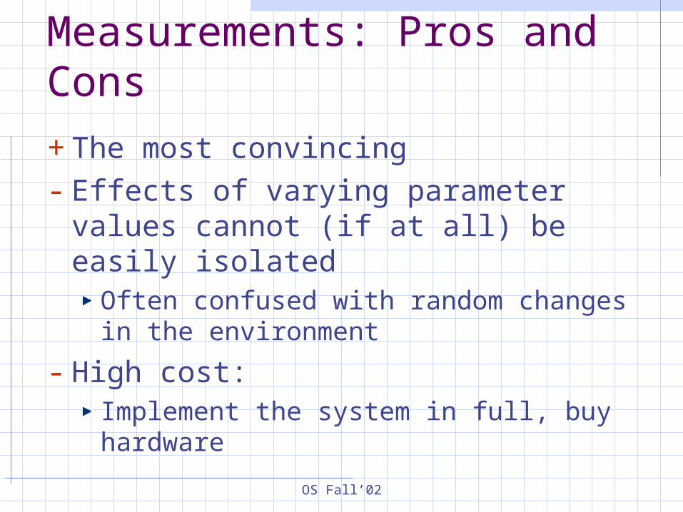
Measurements: Pros and Cons

+The most convincing- Effects of varying parameter values

cannot (if at all) be easily isolatedOften confused with random changes in the environment

- High cost:Implement the system in full, buy hardware

OS Fall’02

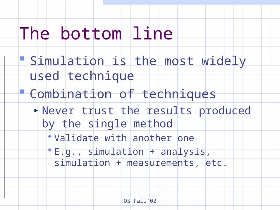
The bottom line Simulation is the most widely used

technique Combination of techniques

Never trust the results produced by the single method Validate with another one E.g., simulation + analysis, simulation +

measurements, etc.

OS Fall’02

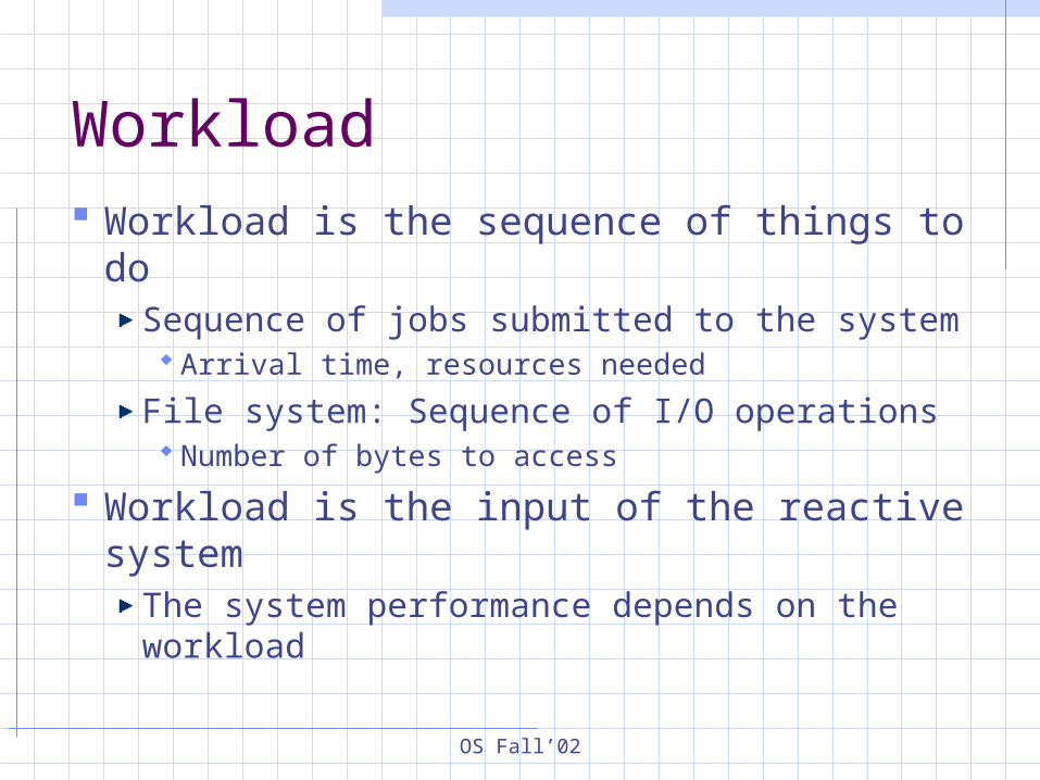
Workload Workload is the sequence of things to

doSequence of jobs submitted to the system Arrival time, resources needed

File system: Sequence of I/O operations Number of bytes to access

Workload is the input of the reactive system

The system performance depends on the workload

OS Fall’02

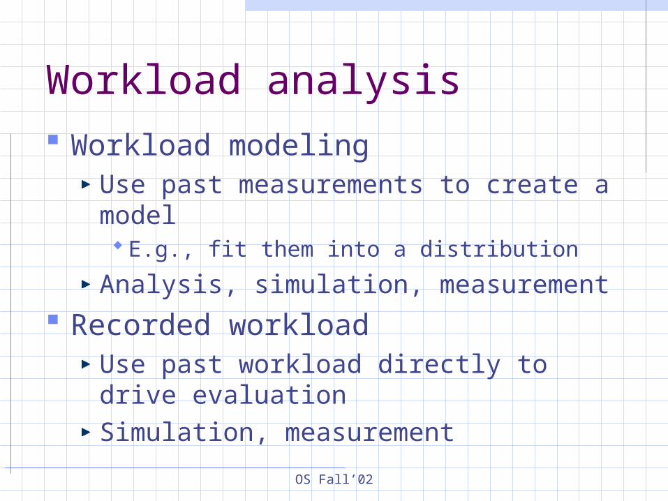
Workload analysis Workload modeling

Use past measurements to create a model E.g., fit them into a distribution

Analysis, simulation, measurement

Recorded workloadUse past workload directly to drive evaluationSimulation, measurement

OS Fall’02

Statistical characterization Every workload item is sampled at

random from the distribution of some random variable

Workload is characterized by a distributionE.g., take all possible job times and fit them to a distribution

OS Fall’02

The Exponential Distribution A lot of low values and a few high

values The distributions of salaries, lifetimes, and

waiting times are often fit the exponential distribution

The distribution ofJob runtimes

Job inter-arrival times

File sizes

OS Fall’02

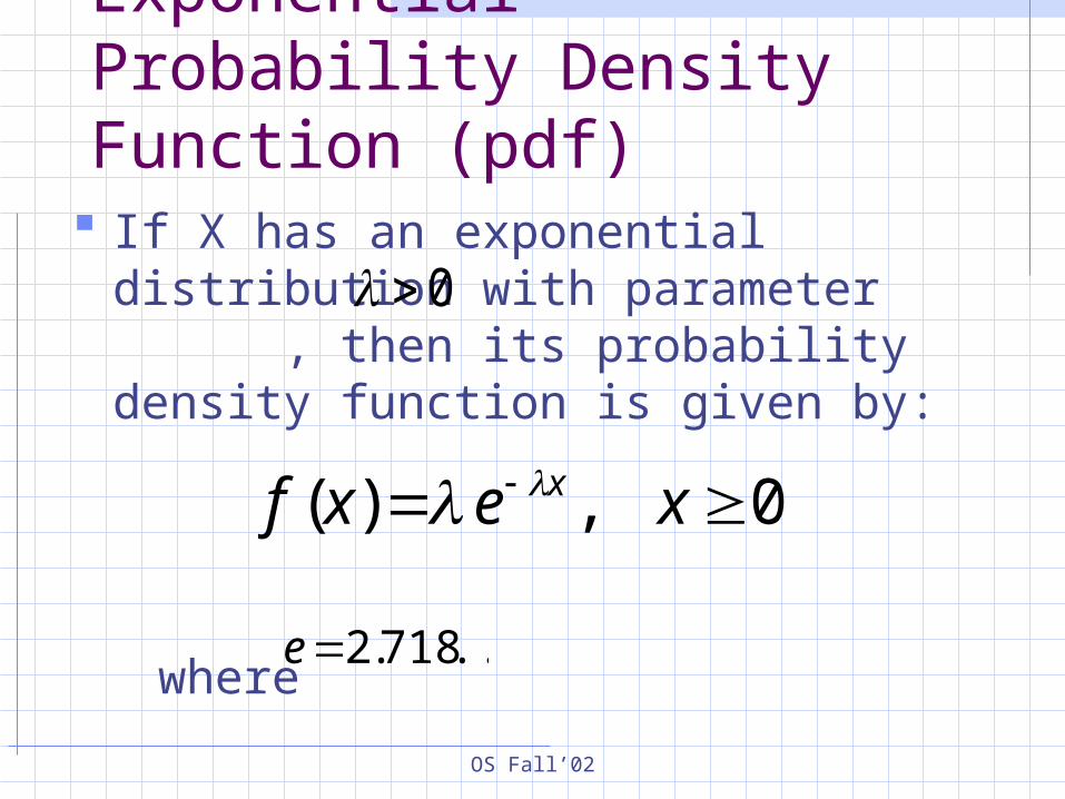
Exponential Probability Density Function (pdf) If X has an exponential distribution with

parameter , then its probability density function is given by:

where...718.2e

0,)( xexf x

0

OS Fall’02

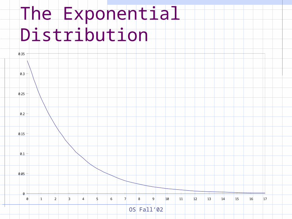
The Exponential Distribution

0

0.05

0.1

0.15

0.2

0.25

0.3

0.35

0 1 2 3 4 5 6 7 8 9 10 11 12 13 14 15 16 17

OS Fall’02

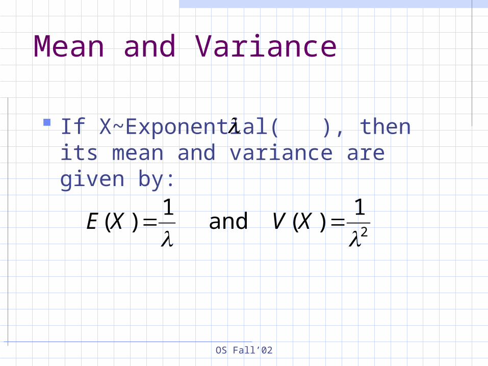
Mean and Variance

If X~Exponential( ), then its mean and variance are given by:

2

1)(and

1)(

XVXE

OS Fall’02

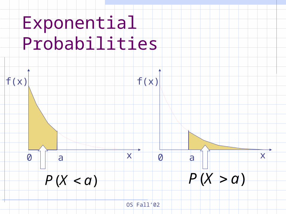
Exponential Probabilities

a x

f(x)

)( aXP

a x

f(x)

)( aXP 0 0

OS Fall’02

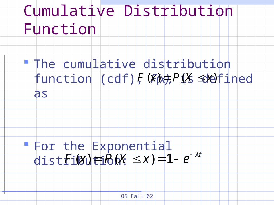
Cumulative Distribution Function

The cumulative distribution function (cdf), F(x), is defined as

For the Exponential distribution:

texXPxF 1)()(

).()( xXPxF

OS Fall’02

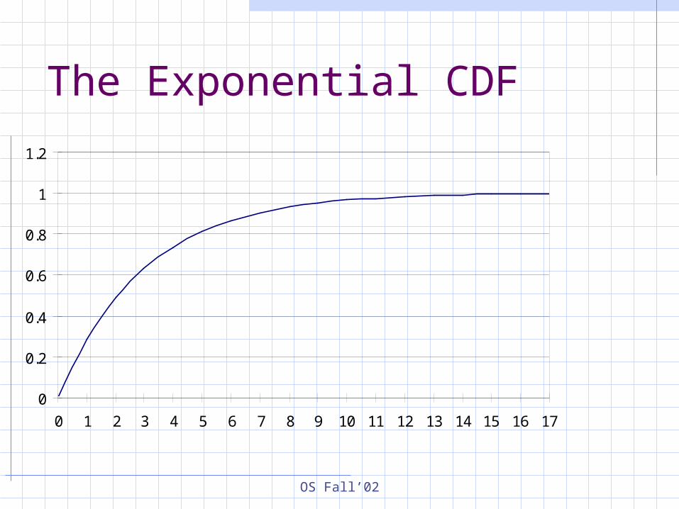
The Exponential CDF

0

0.2

0.4

0.6

0.8

1

1.2

0 1 2 3 4 5 6 7 8 9 10 11 12 13 14 15 16 17

OS Fall’02

Memoryless Property The exponential is the only distribution

with the property that

For modeling runtimes: the probability to run for additional b time units is the same regardless of how much the process has been running already

in average

0, where,)()|( babXPaXbaXP

1

OS Fall’02

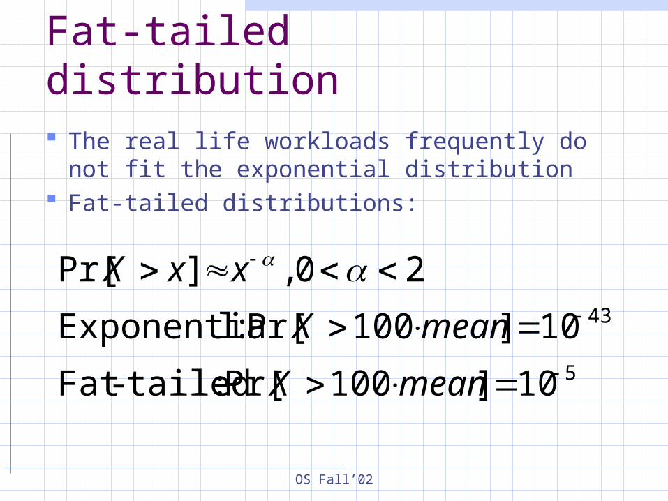
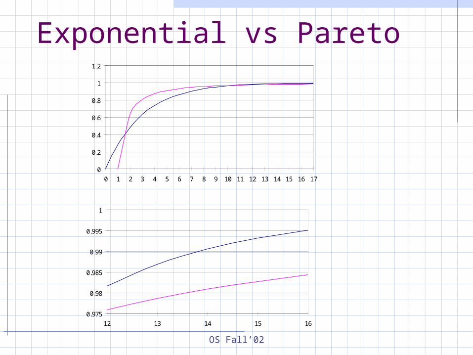
Fat-tailed distribution The real life workloads frequently do not

fit the exponential distribution Fat-tailed distributions:

5

43

10]100Pr[ :tailed-Fat

10]100Pr[ :lExponentia

20 ,]Pr[

meanX

meanX

xxX

OS Fall’02

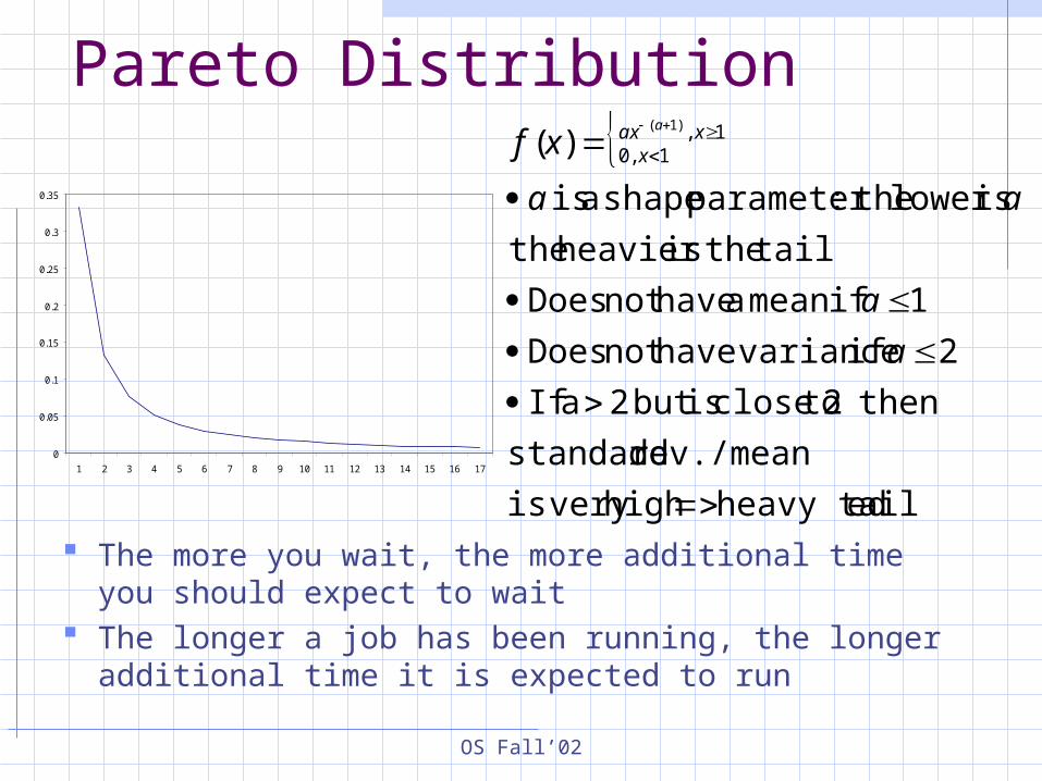
Pareto Distribution

0

0.05

0.1

0.15

0.2

0.25

0.3

0.35

1 2 3 4 5 6 7 8 9 10 11 12 13 14 15 16 17

edheavy tail high very is

dev./mean standard

then 2 toclose isbut 2 a If

2 if variancehavenot Does

1 ifmean a havenot Does

tail theisheavier the

islower the:parameter shape a is

)( 1,1,0

)1(

a

a

aa

xf xaxx

a

The more you wait, the more additional time you should expect to wait

The longer a job has been running, the longer additional time it is expected to run

OS Fall’02

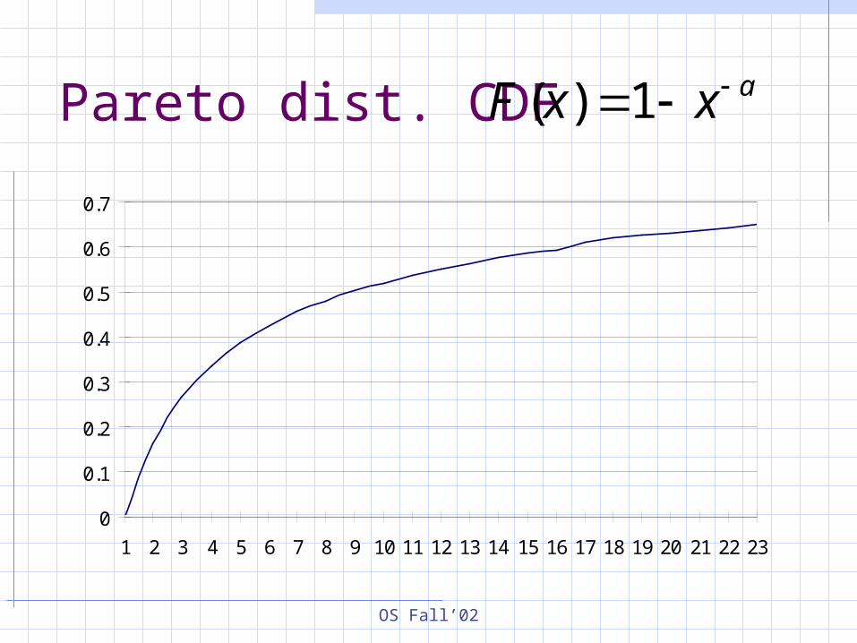
Pareto dist. CDF

0

0.1

0.2

0.3

0.4

0.5

0.6

0.7

1 2 3 4 5 6 7 8 9 10 11 12 13 14 15 16 17 18 19 20 21 22 23

axxF 1)(

OS Fall’02

Exponential vs Pareto

0.975

0.98

0.985

0.99

0.995

1

12 13 14 15 16

0

0.2

0.4

0.6

0.8

1

1.2

0 1 2 3 4 5 6 7 8 9 10 11 12 13 14 15 16 17

OS Fall’02

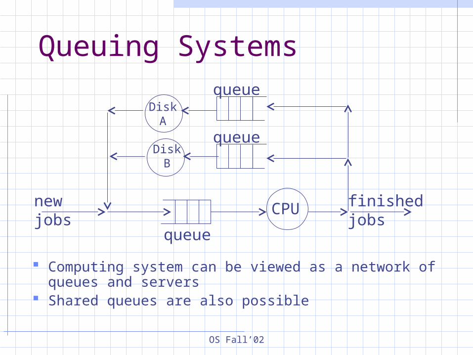
Queuing Systems

Computing system can be viewed as a network of queues and servers

Shared queues are also possible

CPU

DiskA

DiskB

queue

queue

queue

newjobs

finishedjobs

OS Fall’02

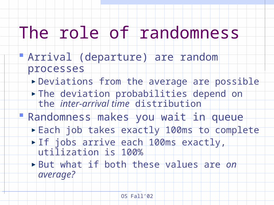
The role of randomness Arrival (departure) are random

processesDeviations from the average are possibleThe deviation probabilities depend on the inter-arrival time distribution

Randomness makes you wait in queueEach job takes exactly 100ms to completeIf jobs arrive each 100ms exactly, utilization is 100%But what if both these values are on average?

OS Fall’02

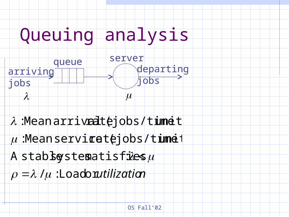
Queuing analysis

arrivingjobs

queue serverdepartingjobs

nutilizatioor Load :/

:satisfies system stableA

unit) (jobs/time rate serviceMean :

unit) (jobs/time rate arrivalMean :

OS Fall’02

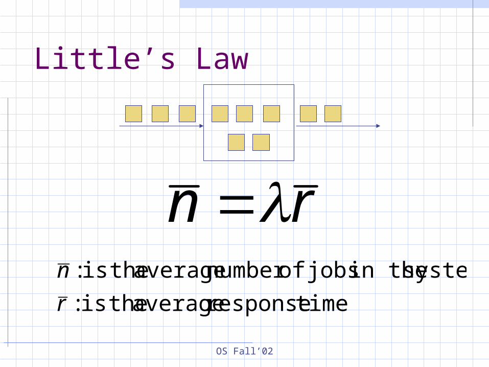
Little’s Law

rn

timeresponse average theis:

system in the jobs ofnumber average theis :

r

n

OS Fall’02

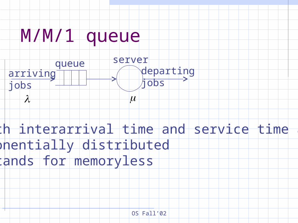
M/M/1 queue

arrivingjobs

queue serverdepartingjobs

Both interarrival time and service time are exponentially distributedM stands for memoryless

OS Fall’02

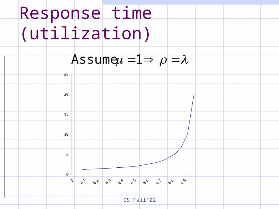
How average response time depends on utilization?

The job arrival and departure are approximated by Poisson processes

The distribution of the number of jobs in the system in the steady state is unique

Use queuing analysis to determine this distribution

Once it is known, can be found Use the Little law to determine

nr

OS Fall’02

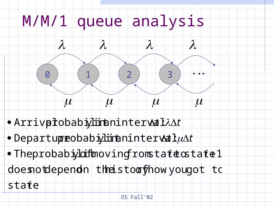
M/M/1 queue analysis

0 1 32

i

i i

tt

tt

state

got toyou how ofhistory on the dependnot does

1 state to state from moving ofy probabilit The

: intervalan in y probabilit Departure

: intervalan in y probabilit Arrival

OS Fall’02

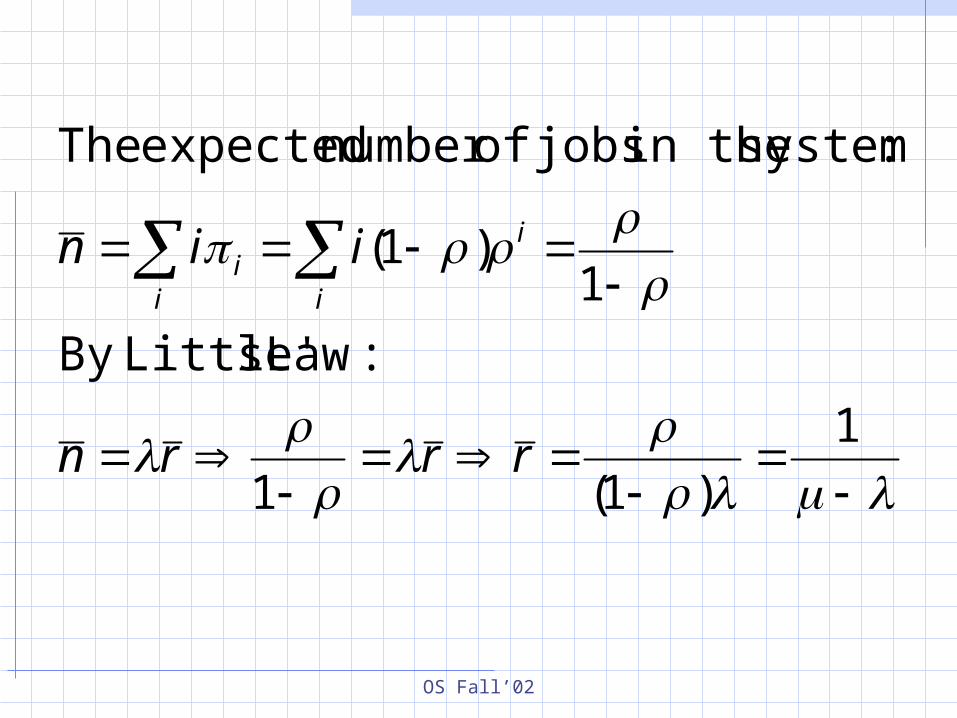
1

)1(1

:Law sLittle'By

1)1(

:system in the jobs ofnumber expected The

rrrn

iin i

iii

OS Fall’02

Response time (utilization)

0

5

10

15

20

25

1 Assume

OS Fall’02

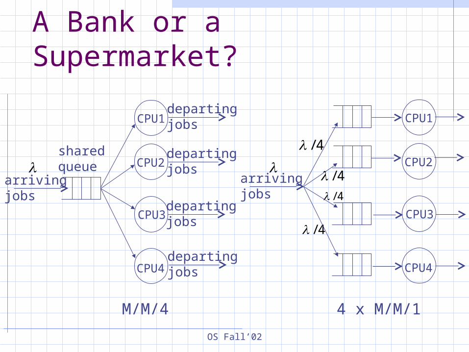
A Bank or a Supermarket?

4/

4/

departingjobs

departingjobs

departingjobs

departingjobs

arrivingjobs

sharedqueue

CPU1

CPU2

CPU3

CPU4

CPU1

CPU2

CPU3

CPU4

arrivingjobs

M/M/4 4 x M/M/1

4/

4/

OS Fall’02

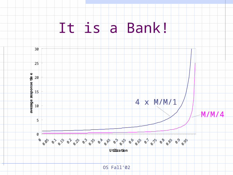
It is a Bank!

0

5

10

15

20

25

30

Utilization

aver

age

resp

on

se t

ime

M/M/4

4 x M/M/1

OS Fall’02

Summary What are the three main performance

evaluation metrics? What are the three main performance

evaluation techniques? What is the most important thing for

performance evaluation? Which workload models do you know? What does make you to wait in

queue? How response time depends on

utilization?

OS Fall’02

To read more Notes Stallings, Appendix A Raj Jain, The Art of Computer

Performance Analysis

OS Fall’02

Next: Processes