Orthogonalizing Penalized Regression

Shifeng Xiong1, Bin Dai2, and Peter Z. G. Qian2

1 Academy of Mathematics and Systems Science

Chinese Academy of Sciences, Beijing 100190

2 Department of Statistics

University of Wisconsin-Madison, Madison, WI 53706

Abstract

Since the penalized likelihood function of the smoothly clipped absolute deviation (SCAD)

penalty is highly non-linear and has many local optima, finding a local solution to achieve the

so-called oracle property is an open problem. We propose an iterative algorithm, called the

OEM algorithm, to fill this gap. The development of the algorithm draws direct impetus from

a missing-data problem arising in design of experiments with an orthogonal complete matrix.

In each iteration, the algorithm imputes the missing data based on the current estimates

of the parameters and updates a closed-form solution associated with the complete data.

By introducing a procedure called active orthogonization, we make the algorithm broadly

applicable to problems with arbitrary regression matrices. In addition to the SCAD penalty,

the proposed algorithm works for other penalties like the MCP, lasso and nonnegative gar-

rote. Convergence and convergence rate of the algorithm are examined. The algorithm has

several unique theoretical properties. For the SCAD and MCP penalties, an OEM sequence

can achieve the oracle property after sufficient iterations. For various penalties, an OEM

sequence converges to a point having grouping coherence for fully aliased regression matri-

ces. For computing the ordinary least squares estimator with a singular regression matrix,

an OEM sequence converges to the Moore-Penrose generalized inverse-based least squares

estimator.

KEY WORDS: Design of experiments; MCP; Missing data; Optimization; Oracle property;

Orthogonal design; SCAD; The EM algorithm; The Lasso.

2Corresponding author: Peter Z. G. Qian. Email: peterq@stat.wisc.edu

1

1 INTRODUCTION

Fan and Li (2001) proposed the smoothly clipped absolute deviation (SCAD) penalty to

achieve simultaneous estimation and variable selection. Consider a linear model

Y = Xβ + ε, (1)

where X = (xij) is the n × p regression matrix, Y ∈ Rn is the response vector, β =

(β1, . . . , βp)′ is the vector of regression coefficients and the distribution of the vector of

random error ε = (ε1, . . . , εn)′ is N(0n, σ2In) with 0n being the nth zero vector and In

being the n × n identity matrix. Throughout, let ‖ · ‖ denote the Euclidean norm. A

regularized least squares estimator of β with this penalty is given by solving

minβ

[‖Y −Xβ‖2 + 2

p∑j=1

Pλ(|βj|)]

, (2)

where for θ > 0,

P ′λ(θ) = λI(θ 6 λ) + (aλ− θ)+I(θ > λ)/(a− 1), (3)

a > 2, λ > 0 is the tuning parameter and I is the indicator function. In order to apply the

penalty Pλ equally on all the variables, X can be standardized so that

n∑i=1

x2ij = 1, for j = 1, . . . , p. (4)

Both theory and computation of the estimator in (2) have been actively studied. On the the-

oretical side, Fan and Li (2001) introduced an important concept, called the oracle property.

An estimator of β having this property can not only select the correct submodel asymptoti-

cally, but also estimate the nonzero coefficients as efficiently as if the correct submodel were

known in advance. On the computational side, existing algorithms for solving this optimiza-

tion problem include local quadratic approximation (Fan and Li 2001; Hunter and Li 2005),

local linear approximation (Zou and Li 2008), the coordinate descent algorithm (Tseng 2001;

2

Tseng and Yun 2009; Breheny and Huang 2010; Mazumder, Friedman, and Hastie 2010) and

the minimization by iterative soft thresholding (MIST) algorithm (Schifano, Strawderman,

and Wells 2010), among others.

Departing from the existing work, we study the SCAD penalty from a new perspective,

targeting on the interface between theory and computing. Fan and Li (2001) proved that

there exists a local solution to (2) with the oracle property. From the optimization viewpoint,

(2) can have many local minima (Huo and Chen 2010) and it is very challenging to find one

of them to achieve the oracle property. To the best of our knowledge, no theoretical results

are available to show that any existing algorithm can provide such a local minimum. We

propose an iterative algorithm, called orthogonalizing EM (OEM), to fill this gap. We will

show in Section 4 that the OEM solution to (2) can indeed achieve the oracle property

under regularity conditions. OEM draws its direct impetus from a missing data problem

with a complete orthogonal design arising in design of experiments. Throughout, a matrix

is orthogonal if its columns are orthogonal. In each iteration, the algorithm imputes the

missing data based on the current estimate of β and updates a closed-form solution to

(2) associated with the complete data. Much beyond this orthogonal design formulation,

the OEM algorithm applies to general data structures by actively orthogonalizing arbitrary

regression matrices.

Though the inspiration of the OEM algorithm stems from the SCAD penalty, it, not

surprisingly, works for the general penalized regression problem:

minβ∈Θ

[‖Y −Xβ‖2 + P (β; λ)], (5)

where β ∈ Θ, Θ is a subset of Rp and λ is the vector of tuning parameters. Besides the

SCAD penalty, choices for P (β; λ) include the ridge regression (Hoerl and Kennard 1970),

the nonnegative garrote (Breiman 1995), the lasso (Tibshirani 1996) and the MCP (Zhang

2010). Algorithms for solving the problem in (5) include those developed in Fu (1998),

Grandvalet (1998), Osborne, Presnell, and Turlach (2000), the LARS algorithm introduced

in Efron, Hastie, Johnstone, and Tibshirani (2004) and the coordinate descent algorithm

3

(Tseng 2001; Friedman, Hastie, Hofling and Tibshirani 2007; Wu and Lange 2008; Tseng

and Yun 2009), and are available in R packages like lars (Hastie and Efron 2011), glmnet

(Friedman, Hastie, and Tibshirani 2011) and scout (Witten and Tibshirani 2011).

In addition to achieving the oracle property for the SCAD and MCP penalties, the OEM

algorithm has several other unique theoretical features. 1. Having grouping coherence: An

estimator β of β in (1) is said to have grouping coherence if it has the same coefficient

for full aliased columns in X (Zou and Hastie 2005). For the lasso, SCAD and MCP,

an OEM sequence converges to a point having grouping coherence. 2. Convergence in

singular case: When X in (1) is singular, the ordinary least squares estimator given by (5)

without any penalty is not unique. For this singular case, an OEM solution, or essentially the

Healy-Westmacott estimator (Healy and Westmacott 1956), converges to the Moore-Penrose

generalized inverse-based least squares estimator.

The remainder of the article will unfold as follows. Section 2 derives the OEM algo-

rithm for a missing data problem with a complete orthogonal design. Section 3 significantly

broadens the applicability of the algorithm by introducing an idea for actively expanding

any regression matrix to an orthogonal matrix. Section 4 establishes the oracle property

of the OEM solution for the SCAD and MCP. Section 5 provides convergence properties of

the OEM algorithm. Section 6 shows that for a regression matrix with full aliased columns,

an OEM sequence for the lasso, SCAD or MCP converges to a solution with grouping co-

herency and illustrates how to use the OEM algorithm to compute the ordinary least squares

estimator for a singular regression matrix. Section 7 provides some discussion.

2 THE OEM ALGORITHM AS A PENALIZED HEALY-

WESTMACOTT PROCEDURE

Orthogonal designs are widely used in science and engineering. Such designs have been

intensively studied in different branches of statistics including design of experiments, infor-

mation theory (MacWilliams and Sloane 1977), liner models, sampling survey and computer

4

experiments. Popular classes of orthogonal designs include orthogonal arrays (Hedayat,

Sloane, and Stufken 1999), orthogonal main-effect plans (Addelman 1962; Wu and Hamada

2009) and orthogonal Latin hypercube designs (Ye 1998; Steinberg and Lin 2006; Bingham,

Sitter, and Tang 2009; Lin, Mukerjee, and Tang 2009; Pang, Liu, and Lin, 2009; Sun, Liu,

and Lin 2009; Lin, Bingham, Sitter, and Tang 2010) from the computer experiments litera-

ture (Santner, Williams, and Notz 2003; Fang, Li, and Sudjianto 2005). In this section, we

motivate the OEM algorithm by using a missing data problem with an orthogonal complete

design. Suppose that the matrix X in (1) for this problem is a submatrix of an m × p

complete orthogonal matrix

Xc = (X ′ ∆′)′, (6)

where ∆ is the (m− n)× p missing matrix. Let

Yc = (Y′, Y′miss)

′ (7)

define the vector of complete observations with Ymiss corresponding to ∆. If Ymiss were

observable, then the ordinary least square estimator of β based on the complete data (Xc,

Yc) has a closed form as Xc is orthogonal. In light of this fact, Healy and Westmacott (1956)

proposed an iterative procedure to compute the ordinary least squares estimator βOLS of β.

In each iteration, their procedure imputes the values of Ymiss and updates the closed-form

ordinary least squares estimator associated with the complete data. The OEM algorithm

follows the same idea but solves (2) with the SCAD penalty. If Ymiss were observable, then

X in (2) and Y can be replaced by Xc and Yc, yielding a closed-form solution to (2). Much

beyond this orthogonal design formulation, we will significantly broaden the applicability of

the algorithm in Section 3 by introducing an idea, called active orthogonalization, to actively

expand any regression matrix into an orthogonal matrix.

Define

A = ∆′∆. (8)

Let (d1, . . . , dp) denote the diagonal elements of X ′cXc. The OEM algorithm for solving the

5

optimization problem in (2) proceeds as follows. Let β(0) be an initial estimate of β. For

k = 0, 1, . . ., impute Ymiss as YI = ∆β(k), let Yc = (Y′, Y′I)′, and solve

β(k+1) = argminβ

[‖Yc −Xcβ‖2 + 2

p∑j=1

Pλ(|βj|)]

(9)

until {β(k)} converges. Letting

u = (u1, . . . , up)′ = X ′Y + Aβ(k), (10)

(9) becomes

β(k+1) = argminβ

[p∑

j=1

(djβ2j − 2ujβj) + 2

p∑j=1

Pλ(|βj|)]

, (11)

which is separable in the dimensions of β. If X in (1) is standardized as in (4) with dj > 1

for all j, (11) has a closed-form

β(k+1)j =

sign(uj)(|uj| − λ

)+/dj, when |uj| 6 (dj + 1)λ,

sign(uj)[(a− 1)|uj| − aλ

]/[(a− 1)dj − 1

], when (dj + 1)λ < |uj| 6 aλdj,

uj/dj, when |uj| > aλdj.

(12)

As pointed out in Dempster, Laird, and Rubin (1977) that the Healy-Westmacott pro-

cedure is essentially an EM algorithm, OEM is an EM algorithm as well. The complete

data Yc = (Y′, Y′miss)

′ in (7) follow a regression model Yc = Xcβ + εc, where εc is from

N(0m, Im). Let βSCAD be a solution to (2), where βSCAD = argmaxβ L(β | Y) and the

penalized likelihood function L(β | Y) is

(2π)−n/2 exp

(−1

2‖Y −Xβ‖2

)exp

[−

p∑j=1

Pλ(|βj|)]

.

6

Given β(k), the E-step of the OEM algorithm for the SCAD is

E[log{L(β|Yc)} | Y,β(k)

]

= −C{‖Y −Xβ‖2 + E

(‖Ymiss −Xβ‖2 | β(k))

+ 2

p∑j=1

Pλ(|βj|)}

= −C{n + ‖Y −Xβ‖2 + ‖∆β(k) −∆β‖2 + 2

p∑j=1

Pλ(|βj|)}

for some constant C > 0. Define

QSCAD(β | β(k)) = ‖Y −Xβ‖2 + ‖∆β(k) −∆β‖2 + 2

p∑j=1

Pλ(|βj|). (13)

The M-step of the OEM algorithm for the SCAD is

β(k+1) = arg minβ

QSCAD(β | β(k)),

which is equivalent to (11).

For the general penalized regression problem in (5), the M-step of the OEM algorithm

becomes

β(k+1) = arg minβ∈Θ

Q(β | β(k)), (14)

where Q replaces QSCAD in (13) for the corresponding penalty function. If Θ and P in (5) are

decomposable as Θ =∏p

j=1 Θj and P (β; λ) =∑p

j=1 Pj(βj; λ), similarly to (11), (14) reduces

to p one-dimensional problems

β(k+1)j = argmin

βj∈Θj

[djβ

2j − 2ujβj + Pj(βj; λ)

], for j = 1, . . . , p, (15)

with u = (u1, . . . , up)′ defined in the same way as in (10). This shortcut applies to the

following penalties:

7

1. The lasso (Tibshirani 1996), where Θj = R,

Pj(βj; λ) = 2λ|βj|, (16)

and (15) becomes

β(k+1)j = sign(uj)

( |uj| − λ

dj

)

+

. (17)

Here, for a ∈ R, (a)+ denotes max{a, 0}.

2. The nonnegative garrote (Breiman 1995), where Θj = {x : xβj > 0}, Pj(βj; λ) =

2λβj/βj, βj is the ordinary least squares estimator of βj, and (15) becomes

β(k+1)j =

(ujβj − λ

djβ2j

)

+

βj.

3. The elastic-net (Zou and Hastie 2005), where Θj = R,

Pj(βj; λ) = 2λ1|βj|+ λ2β2j . (18)

and (15) becomes

β(k+1)j = sign(uj)

( |uj| − λ1

dj + λ2

)

+

. (19)

5. The MCP (Zhang 2010), where Θj = R, Pj(βj; λ) = 2Pλ(|βj|), and

P ′λ(θ) = (λ− θ/a)I(θ 6 aλ) (20)

with a > 1 and θ > 0. If X in (1) is standardized as in (4) with dj > 1 for all j, (15)

becomes

β(k+1)j =

sign(uj)a(|uj| − λ

)+/(adj − 1), when |uj| 6 aλdj,

uj/dj, when |uj| > aλdj

(21)

8

6. The “Berhu” penalty (Owen 2006), where Θj = R, Pj(βj; λ) = 2λ{|βj|I(|βj| < δ) +

(β2j + δ2)I(|βj| > δ)/(2δ)

}for some δ > 0, and (15) becomes

β(k+1)j =

sign(uj)(|uj| − λ

)+/dj, when |uj| < λ + djδ,

ujδ/(λ + djδ), when |uj| > λ + djδ.

Obviously, if the penalty on β disappears, the OEM algorithm reduces to the Healy-

Westmacott procedure. Quite interestingly, Theorem 6 in Section 5 shows that, for the same

X and Y in (1), the OEM algorithm for the elastic-net and lasso numerically converges

faster than the Healy-Westmacott procedure.

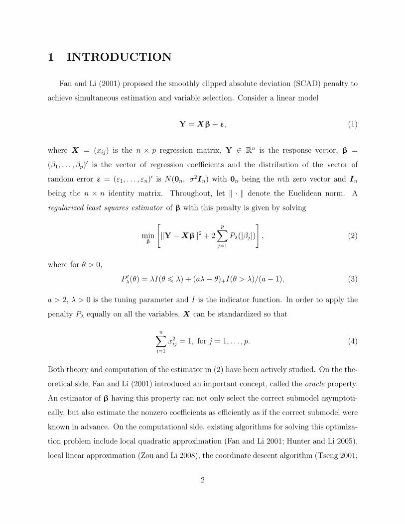
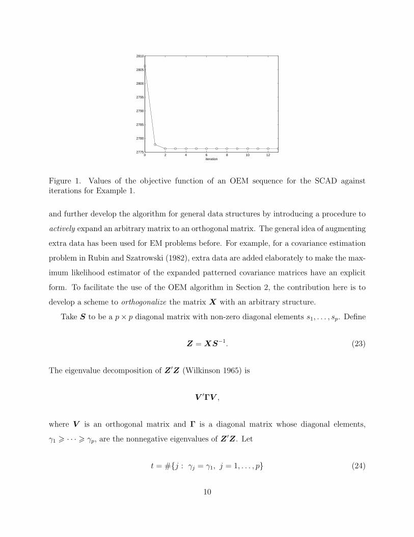
Example 1. For the model in (1), let the complete matrix Xc be a fractional factorial

design from Xu (2009) with 4096 runs in 30 factors. Clearly, Xc is an orthogonal design.

Let X in (1) be the submatrix of Xc consisting of the first 3000 rows and let Y be generated

with σ = 1 and

βj = (−1)j exp[− 2(j − 1)/20

]for j = 1, . . . , p. (22)

Here, p = 30 and n = 3000. Assume the response values corresponding to the last 1096 rows

of Xc are missing. We used the OEM algorithm to solve the optimization problem in (2) with

an initial value β(0) = 0 and a criterion to stop when relative changes in all coefficients are

less than 10−6. For λ = 1 and a = 3.7 in (3), Figure 1 plots values of the objective function

in (2) of the OEM sequence against iteration numbers, where the algorithm converges at

iteration 13.

3 THE GENERAL FORMULATION WITH ACTIVE

ORTHOGONALIZATION

The OEM algorithm in Section 2 was derived for a missing-data problem where X in (1)

is imbedded in a pre-specified orthogonal matrix. We drop this assumption in this section

9

0 2 4 6 8 10 122775

2780

2785

2790

2795

2800

2805

2810

iteration

Figure 1. Values of the objective function of an OEM sequence for the SCAD againstiterations for Example 1.

and further develop the algorithm for general data structures by introducing a procedure to

actively expand an arbitrary matrix to an orthogonal matrix. The general idea of augmenting

extra data has been used for EM problems before. For example, for a covariance estimation

problem in Rubin and Szatrowski (1982), extra data are added elaborately to make the max-

imum likelihood estimator of the expanded patterned covariance matrices have an explicit

form. To facilitate the use of the OEM algorithm in Section 2, the contribution here is to

develop a scheme to orthogonalize the matrix X with an arbitrary structure.

Take S to be a p× p diagonal matrix with non-zero diagonal elements s1, . . . , sp. Define

Z = XS−1. (23)

The eigenvalue decomposition of Z ′Z (Wilkinson 1965) is

V ′ΓV ,

where V is an orthogonal matrix and Γ is a diagonal matrix whose diagonal elements,

γ1 > · · · > γp, are the nonnegative eigenvalues of Z ′Z. Let

t = #{j : γj = γ1, j = 1, . . . , p} (24)

10

denote the number of the γj equal to γ1. For example, if γ1 = γ2 and γ1 > γj for j = 3, . . . , p,

then t = 2. Define

B = diag(γ1 − γt+1, . . . , γ1 − γp) (25)

and

∆ = B1/2V 1S, (26)

where V 1 is the submatrix of V consisting of the last p− t rows. Let Xc be the augmented

matrix of ∆ and X.

Lemma 1. The matrix Xc constructed above is orthogonal.

Proof. Note that

X ′cXc = X ′X + ∆′∆,

which, by plugging (25) and (26), becomes

S[Z ′Z + V ′(γ1Ip − Γ)V ]S = γ1S2. (27)

Now, because

γ1Ip − Γ =

0 0

0 B

,

(27) is orthogonal, which completes the proof.

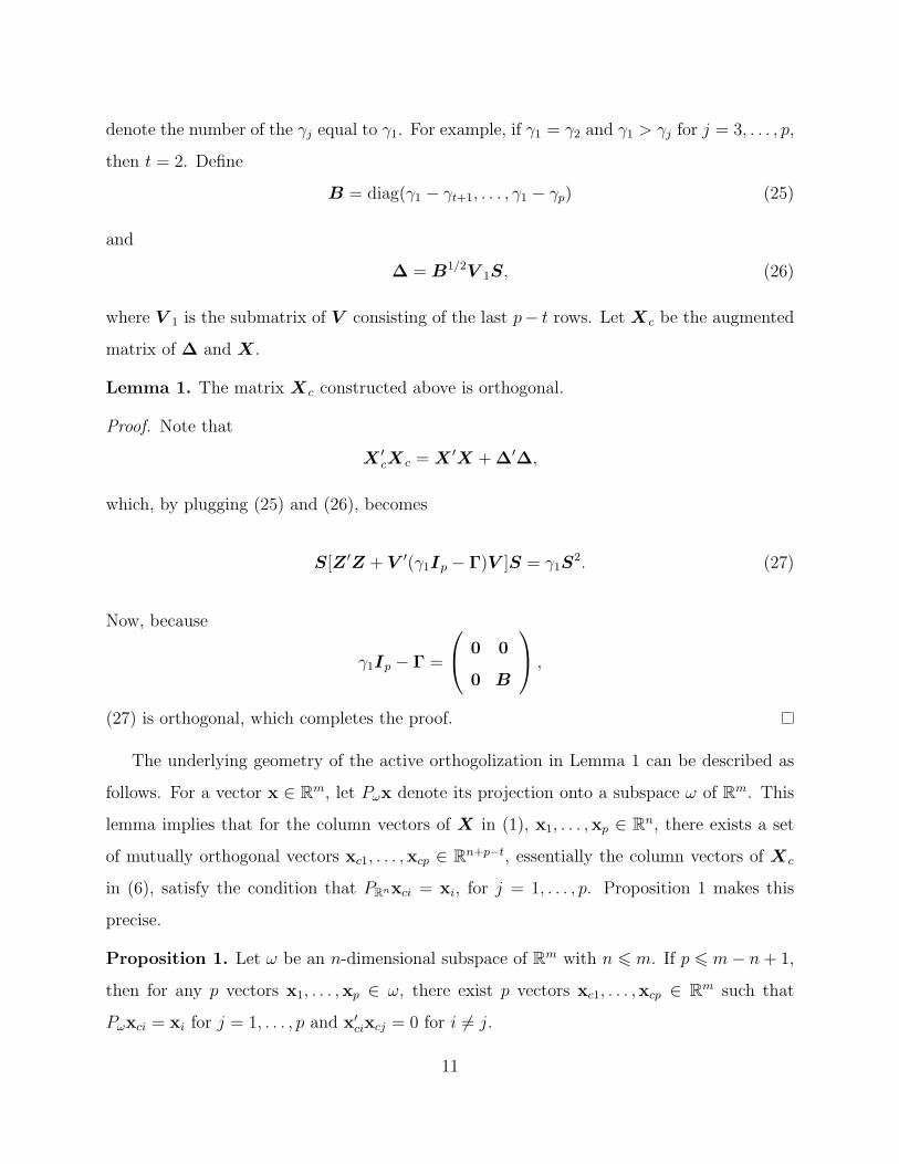
The underlying geometry of the active orthogolization in Lemma 1 can be described as

follows. For a vector x ∈ Rm, let Pωx denote its projection onto a subspace ω of Rm. This

lemma implies that for the column vectors of X in (1), x1, . . . ,xp ∈ Rn, there exists a set

of mutually orthogonal vectors xc1, . . . ,xcp ∈ Rn+p−t, essentially the column vectors of Xc

in (6), satisfy the condition that PRnxci = xi, for j = 1, . . . , p. Proposition 1 makes this

precise.

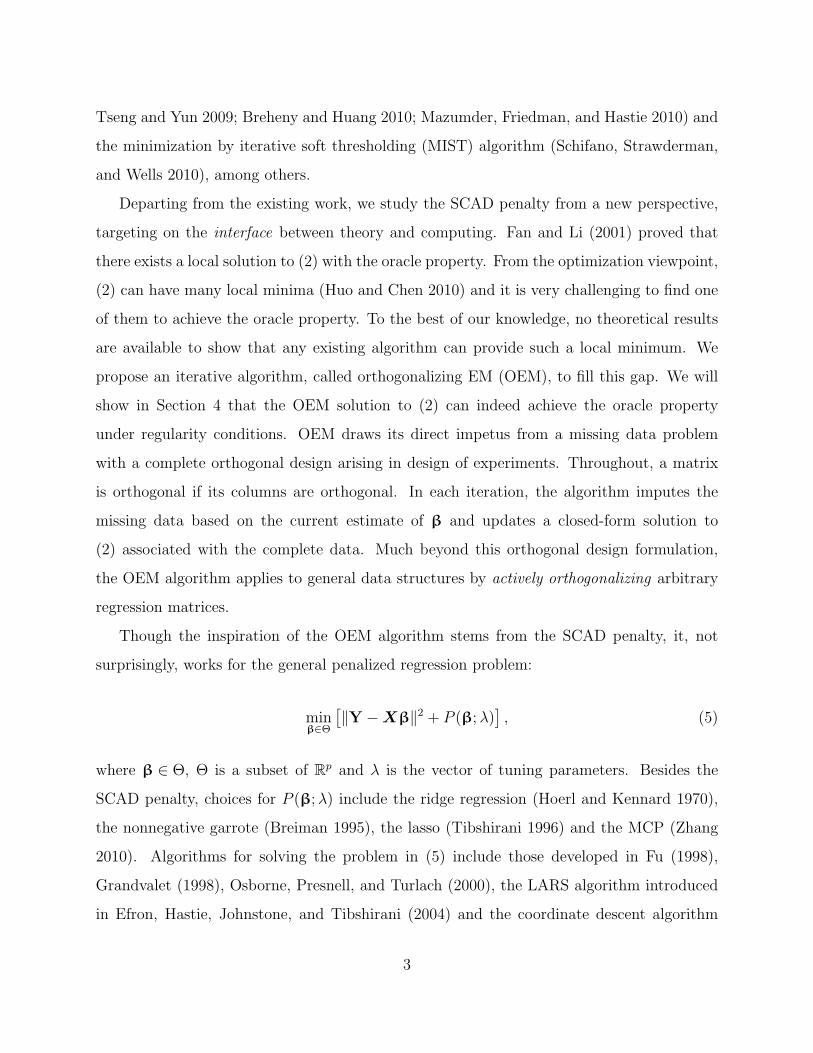
Proposition 1. Let ω be an n-dimensional subspace of Rm with n 6 m. If p 6 m− n + 1,

then for any p vectors x1, . . . ,xp ∈ ω, there exist p vectors xc1, . . . ,xcp ∈ Rm such that

Pωxci = xi for j = 1, . . . , p and x′cixcj = 0 for i 6= j.

11

yx

2

xc2

z

O

xc1

x1

x

Figure 2. Expand two two-dimensional vectors x1 and x2 to two three-dimensional vectorsxc1 and xc2 with x′c1xc2 = 0.

Figure 2 expands two vectors x1 and x2 in R2 to two orthogonal vectors xc1 and xc2 in R3.

Now, if Xc from Lemma 1 is treated as the complete matrix defined in (6), the OEM

algorithm in Section 2 follows through immediately.

When using the OEM algorithm to solve (5), in (10) instead of computing ∆ in (26),

one may compute A = ∆′∆ and the diagonal entries d1, . . . , dp of X ′cXc. Note that

A = γ1S2 −X ′X (28)

and

dj = γ1s2j for j = 1, . . . , p, (29)

where S and Z are defined in (23) and γ1 is the largest eigenvalue of Z ′Z = S−1X ′XS−1.

One way to compute γ1 is to use the power method (Wilkinson 1965) described below.

Given a nonzero initial vector a(0) ∈ Rp, let γ(0)1 = ‖a(0)‖. For k = 0, 1, ..., compute

a(k+1) = X ′Xa(k)/γ(k)1 and γ

(k+1)1 = ‖a(k+1)‖ until convergence. If a(0) is not an eigenvector

12

of any γj that does not equal γ1, then γ(k)1 converges to γ1. For t defined in (24), the

convergence rate is linear (Watkins 2002) specified by

limk→∞

‖γ(k+1)1 − γ1‖‖γ(k)

1 − γ1‖=

γt+1

γ1

.

An easy way to make A = ∆′∆ in (28) positive definite is to replace B in (25) by

B = diag(d− γt+1, . . . , d− γp)

with d > γ1, which changes (28) and (29) to

A = dS2 −X ′X (30)

and

dj = ds2j , for j = 1, . . . , p, (31)

respectively. If d > γ1, then A = ∆′∆ is positive definite.

Remark 1. The matrix S in (23) can be chosen flexibly. One possibility is to use S = Ip

so that

X ′X + ∆′∆ = dIp (32)

with d > γ1, and Xc/√

d is standardized as in (4).

Example 2. Suppose that X in (1) is orthogonal. Take

S = diag

[(

n∑i=1

x2i1)

1/2, . . . , (n∑

i=1

x2ip)

1/2

]. (33)

Since t = p, ∆ in (26) is empty. This result indicates the active orthogonalization procedure

will not overshoot: if X is orthogonal already, it adds no row.

13

Example 3. Let

X =

0 0 3/2

−4/3 −2/3 1/6

2/3 4/3 1/6

−2/3 2/3 −7/6

.

If S = I3, (26) gives ∆ = (−2/√

3, 2/√

3, 1/√

3).

Example 4. Consider a two-level design in three factors, A, B and C:

−1 −1 −1

−1 1 1

1 −1 1

1 1 −1

.

The regression matrix including all main effects and two-way interactions is

X =

−1 −1 −1 1 1 1

−1 1 1 −1 −1 1

1 −1 1 −1 1 −1

1 1 −1 1 −1 −1

,

where the last three columns for the interactions are fully aliased with the first three columns

for the main effects. For S = I3, (26) gives

∆ =

0 −2 0 0 −2 0

0 0 −2 −2 0 0

−2 0 0 0 0 −2

.

The elements in ∆ are chosen flexibly, not restricted to ±1.

Example 5. Consider a 1000 × 10 random matrix X = (xij) with entries independently

14

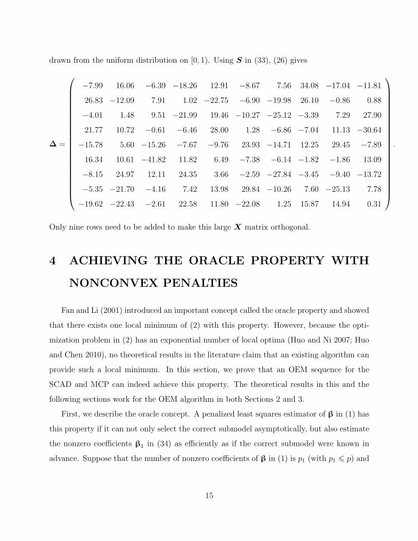
drawn from the uniform distribution on [0, 1). Using S in (33), (26) gives

∆ =

−7.99 16.06 −6.39 −18.26 12.91 −8.67 7.56 34.08 −17.04 −11.81

26.83 −12.09 7.91 1.02 −22.75 −6.90 −19.98 26.10 −0.86 0.88

−4.01 1.48 9.51 −21.99 19.46 −10.27 −25.12 −3.39 7.29 27.90

21.77 10.72 −0.61 −6.46 28.00 1.28 −6.86 −7.04 11.13 −30.64

−15.78 5.60 −15.26 −7.67 −9.76 23.93 −14.71 12.25 29.45 −7.89

16.34 10.61 −41.82 11.82 6.49 −7.38 −6.14 −1.82 −1.86 13.09

−8.15 24.97 12.11 24.35 3.66 −2.59 −27.84 −3.45 −9.40 −13.72

−5.35 −21.70 −4.16 7.42 13.98 29.84 −10.26 7.60 −25.13 7.78

−19.62 −22.43 −2.61 22.58 11.80 −22.08 1.25 15.87 14.94 0.31

.

Only nine rows need to be added to make this large X matrix orthogonal.

4 ACHIEVING THE ORACLE PROPERTY WITH

NONCONVEX PENALTIES

Fan and Li (2001) introduced an important concept called the oracle property and showed

that there exists one local minimum of (2) with this property. However, because the opti-

mization problem in (2) has an exponential number of local optima (Huo and Ni 2007; Huo

and Chen 2010), no theoretical results in the literature claim that an existing algorithm can

provide such a local minimum. In this section, we prove that an OEM sequence for the

SCAD and MCP can indeed achieve this property. The theoretical results in this and the

following sections work for the OEM algorithm in both Sections 2 and 3.

First, we describe the oracle concept. A penalized least squares estimator of β in (1) has

this property if it can not only select the correct submodel asymptotically, but also estimate

the nonzero coefficients β1 in (34) as efficiently as if the correct submodel were known in

advance. Suppose that the number of nonzero coefficients of β in (1) is p1 (with p1 6 p) and

15

partition β as

β = (β′1,β′2)′, (34)

where β2 = 0 and no component of β1 is zero. Divide the regression matrix X in (1) to

(X1 X2) with X1 corresponding to β1. If all the variables that influence the response in

(1) are known, an oracle estimator can be given as β = (β′1, β

′2)′ with β2 = 0, where

β1 − β1 ∼ N(0, σ2(X ′1X1)

−1).

We need several assumptions.

Assumption 1. As n →∞,

X ′Xn

→ Σ =

Σ1 Σ12

Σ21 Σ2

,

where Σ is positive definite and Σ1 is p1 × p1. Furthermore, X/√

n is standardized such

that each entry on the diagonal of X ′X/n is 1, and X ′X/n + ∆′∆ = dIp with d > γ1,

where d = O(1) and γ1 is the largest eigenvalue of X ′X/n.

Assumption 2. The tuning parameter λ = λn in (3) satisfies the condition that, as n →∞,

λn/n → 0 and λn/√

n →∞.

Let {β(k), k = 0, 1, . . . , } be the OEM sequence from (12) for the SCAD with a fixed

a > 2 in (3). We need an assumption on k = kn. Let η be the largest eigenvalue of

Ip1−X ′1X1/(nd). Under Assumption 1, η tends to a limit lying between 0 and 1 as n →∞.

Assumption 3. As n →∞, ηknλn/√

n → 0 and k2n exp(−c(λn/

√n)2) → 0 for any c > 0.

One choice for kn to satisfy Assumption 3 is

kn =

(λn√n

)ν

for some ν > 0.

Under Assumption 2, kn →∞ as n →∞.

16

Under the above assumptions, Theorem 1 shows that β(k) = (β(k)′1 , β

(k)′2 )′ can achieve the

oracle property.

Theorem 1. Suppose that Assumption 1-3 hold. If β(0) = (X ′X)−1X ′Y, then as n →∞,

(i) P(β(k)2 = 0) → 1;

(ii)√

n(β(k)1 − β1) → N(0, σ2Σ−1

1 ) in distribution.

The proof of Theorem 1 is deferred to the Appendix.

Remark 2. From (60) in the proof of Theorem 1, for k = 1, 2, . . ., β(k) is consistent in

variable selection. That is, P(β(k)j 6= 0 for j = 1, . . . , p1) → 1 and P(β

(k)2 = 0) → 1 as

n →∞.

Remark 3. The proof of Theorem 1 uses the convergence rates of P(Ak), P(Bk) and P(Chk ).

If an OEM sequence satisfies the condition that β(k+1)j = 0 when |uj| < λ and β

(k+1)j = uj/d

when |uj| > cλ for some c = O(1), then P(Ak+1) = P(|uj| < λ) and P(Bk+1) = P(|uj| > cλ).

Since an OEM sequence for the MCP satisfies the above condition, an argument very similar

to the proof in the Appendix shows that the convergence rates of P(Ak), P(Bk) and P(Chk )

for the MCP are the same as those with the SCAD. Thus, under Assumption 1-3, Theorem 1

holds for the MCP with a fixed a > 1 in (20).

Huo and Chen (2010) showed that, for the SCAD penalty, solving the global minimum

of (5) leads to an NP-hard problem. Theorem 1 indicates that as far as the oracle property

is concerned, the local solution given by OEM will suffice.

5 CONVERGENCE OF THE OEM ALGORITHM

In this section, we derive theoretical results on convergence properties of the OEM algo-

rithm and compare the convergence rates of OEM for the ordinary least squares estimator

and the elastic-net and lasso. The general penalty in (5) is considered here. Our derivations

employs the main tool in Wu (1983) in conjunction with special properties of the penalties

mentioned in Section 2.

17

We make several assumptions for Θ and P (β; λ) in (5).

Assumption 4. The parameter space Θ is a closed convex subset of Rp.

Assumption 5. For a fixed λ, the penalty P (β; λ) → +∞ as ‖β‖ → +∞.

Assumption 6. For a fixed λ, the penalty P (β; λ) is continuous with respect to β ∈ Θ.

All penalties discussed in Section 2 satisfy these assumptions. The assumptions cover the

case in which the iterative sequence {β(k)} defined in (14) may fall on the boundary of Θ

(Nettleton 1999), like the nonnegative garrote (Breiman 1995) and the nonnegative lasso

(Efron et al. 2004). The bridge penalty (Frank and Friedman 1993) in (37) also satisfies the

above assumptions.

For the model in (1), denote the objective function in (5) by

l(β) = ‖Y −Xβ‖2 + P (β; λ). (35)

For some penalizes like the bridge, it may be numerically infeasible to perform the M-step

in (14). For this situation, following the generalized EM algorithm in Dempster, Laird, and

Rubin (1977), we define a generalized OEM algorithm to be an iterative scheme

β(k) → β(k+1) ∈M(β(k)), (36)

where β →M(β) ⊂ Θ is a point-to-set map such that

Q(φ | β) 6 Q(β | β), for all φ ∈M(β).

Here, Q is given by replacing the SCAD with P (β; λ) in (13). The OEM sequence defined

by (14) is a special case of (36). For example, the generalized OEM algorithm can be used

for the bridge penalty, where Θj = R and

Pj(βj; λ) = λ|βj|a (37)

18

for some a ∈ (0, 1) in (5). Since the solution to (15) with the bridge penalty has no closed

form, one may use one-dimensional search to compute β(k+1)j that satisfies (36). By Assump-

tion 1, {β ∈ Θ : l(β) 6 l(β(0))} is compact for any l(β(0)) > −∞. By Assumption 6, M is

a closed point-to-set map (Zangwill 1969; Wu 1983).

The objective functions of the EM algorithms in the literature like those discussed in

Wu (1983), Green (1990) and McLachlan and Krishnan (2008) are typically continuously

differentiable. This condition does not hold for the objective function in (5) with the lasso

and other penalties. A more general definition of stationary points is needed here. We call

β ∈ Θ a stationary point of l if

lim inft→0+

l((1− t)β + tφ

)− l(β)

t> 0 for all φ ∈ Θ.

Let S denote the set of stationary points of l. Analogous to Theorem 1 in Wu (1983) on the

global convergence of the EM algorithm, we have the following result.

Theorem 2. Let {β(k)} be a generalized OEM sequence generated by (36). Suppose that

l(β(k+1)) < l(β(k)) for all β(k) ∈ Θ \ S. (38)

Then all limit points of {β(k)} are elements of S and l(β(k)) converges monotonically to

l∗ = l(β∗) for some β∗ ∈ S.

Theorem 3. If β∗ is a local minimum of Q(β | β∗), then β∗ ∈ S.

This theorem follows from the fact that l(β)−Q(β | β∗) is differentiable and

∂[l(β)−Q(β | β∗)]

∂β

∣∣∣β=β

∗ = 0.

Remark 4. By Theorem 3, if β(k) /∈ S, then β(k) cannot be a local minimum of Q(β | β(k)).

Thus, there exists at least one point β(k+1) ∈M(β(k)) such that Q(β(k+1) | β(k)) < Q(β(k) |β(k)) and therefore satisfies the condition in (38). As a special case, an OEM sequence

generated by (14) satisfies (38) in Theorem 2.

19

Next, we consider the convergence of a generalized OEM sequence {β(k)} in (36). By

Theorem 3, such results will automatically hold for an OEM sequence as well. If the penalty

function P (β; λ) is convex and l(β) has a unique minimum, Theorem 4 shows that {β(k)}converges to the global minimum.

Theorem 4. Let {β(k)} be defined in Theorem 2. Suppose that l(β) in (35) is a convex

function on Θ with a unique minimum β∗ and that (38) holds for {β(k)}. Then β(k) → β∗

as k →∞.

Proof. We only need to show that S = {β∗}. For φ ∈ Θ with φ 6= β∗ and t > 0, we have

l((1− t)φ + tβ∗

)− l(β∗)

t6 tl(β∗) + (1− t)l(φ)− l(φ)

t= l(β∗)− l(φ) < 0.

This implies φ /∈ S.

Theorem 5 discusses the convergence of an OEM sequence {β(k)} for more general penal-

ties. For a ∈ R, define S(a) = {φ ∈ S : l(φ) = a}. From Theorem 2, all limit points of an

OEM sequence are in S(l∗), where l∗ is the limit of l(β(k)) in Theorem 2. Theorem 5 states

that the limit point is unique under certain conditions.

Theorem 5. Let {β(k)} be a generalized OEM sequence generated by (36) with ∆′∆ > 0.

If (38) holds, then all limit points of {β(k)} are in a connected and compact subset of S(l∗).

In particular, if the set S(l∗) is discrete in that its only connected components are singletons,

then β(k) converges to some β∗ in S(l∗) as k →∞.

Proof. Note that Q(β(k+1) | β(k)) = l(β(k+1)) + ‖∆β(k+1) − ∆β(k)‖2 6 Q(β(k) | β(k)) =

l(β(k)). By Theorem 2, ‖∆β(k+1) −∆β(k)‖2 6 l(β(k)) − l(β(k+1)) → 0 as k → ∞. Thus,

‖β(k+1) −β(k)‖ → 0. This theorem now follows immediately from Theorem 5 of Wu (1983).

Since the bridge, SCAD and MCP penalties all satisfy the condition that S(l∗) is discrete,

an OEM sequence for any of them converges to the stationary points of l. Theorem 5 is

obtained under the condition ∆′∆ > 0. Since the error ε in (1) has a continuous distribution,

20

it is easy to show that Theorem 5 holds with probability one if ∆′∆ is singular when d defined

in (30) and (31) equals γ1.

We now derive the convergence rate of the OEM sequence in (14). Following Dempster,

Laird, and Rubin (1977), write

β(k+1) = M(β(k)),

where the map M(β) = (M1(β), . . . , Mp(β))′ is defined by (14). We capture the convergence

rate of the OEM sequence {β(k)} through M. Assume that (32) holds for d > γ1, where

γ1 is the largest eigenvalue of X ′X. For the active orthogolization in (30) and (31), taking

S = Ip satisfies this assumption; see Remark 1.

Let β∗ be the limit of the OEM sequence {β(k)}. As in Meng (1994), we call

R = lim supk→∞

‖β(k+1) − β∗‖‖β(k) − β∗‖ = lim sup

k→∞

‖M(βk)−M(β∗)‖‖β(k) − β∗‖ (39)

the global rate of convergence for the OEM sequence. If there is no penalty in (5), i.e.,

computing the ordinary least squares estimator, the global rate of convergence R in (39)

becomes the largest eigenvalue of J(β∗), denoted by R0, where J(φ) is the p× p Jacobian

matrix for M(φ) having (i, j)th entry ∂Mi(φ)/∂φj. If (32) holds, then J(β∗) = A/d with

A = ∆′∆. Thus,

R0 =d− γp

d. (40)

For (5), the penalty function P (β; λ) typically is not sufficiently smooth and R in (39)

does not have an analytic form. Theorem 6 gives an upper bound of Rnet, the value of R for

the elastic-net penalty in (18) with λ1, λ2 > 0.

Theorem 6. For ∆ from (6), if (32) holds, then RNET 6 R0.

Proof. Let xj denote the jth column of X and aj denote the jth column of A = ∆′∆,

respectively. For an OEM sequence for the elastic-net, by (19),

Mj(β) = f(x′jY + a′jβ), for j = 1, . . . , p,

21

where

f(u) = sign(u)

( |u| − λ1

d + λ2

)

+

.

For j = 1, . . . , p, observe that

|Mj(β(k))−Mj(β

∗)|‖β(k) − β∗‖ =

|f(x′jY + a′jβ(k))− f(x′jY + a′jβ

∗)||(x′jY + a′jβ

(k))− (x′jY + a′jβ∗)|

· |(x′jY + a′jβ

(k))− (x′jY + a′jβ∗)|

‖β(k) − β∗‖

6 1

d· |a

′j(β

(k) − β∗)|‖β(k) − β∗‖ .

Thus,‖M(β(k))−M(β∗)‖

‖β(k) − β∗‖ 6 1

d· ‖A(β(k) − β∗)‖‖β(k) − β∗‖ 6 d− γp

d.

This completes the proof.

Remark 5. Theorem 6 indicates that, for the same X and Y in (1), the OEM solution for

the elastic-net converges faster than its counterpart for the ordinary least squares. Since the

lasso is a special case of the elastic-net with λ2 = 0 in (18), this theorem holds for the lasso

as well.

Remark 6. From (40) and Theorem 6, the convergence rate of the OEM algorithm depends

on the ratio of the smallest eigenvalue, γp, and the largest eigenvalue, γ1, of X ′X. This rate

is the fastest when γ1 = γp, i.e., if X is orthogonal and standardized. This result suggests

that OEM converges faster if X is orthogonal or nearly orthogonal like from a supersaturated

design or a nearly orthogonal Latin hypercube design (Owen 1994; Tang 1998). This result is

in agreement with the recent finding in the design of experiments community that the use of

orthogonal or nearly orthogonal designs can significantly improve the accuracy of penalized

variable selection methods (Phoa, Pan, and Xu 2009; Deng, Lin, and Qian 2010; Zhu 2011).

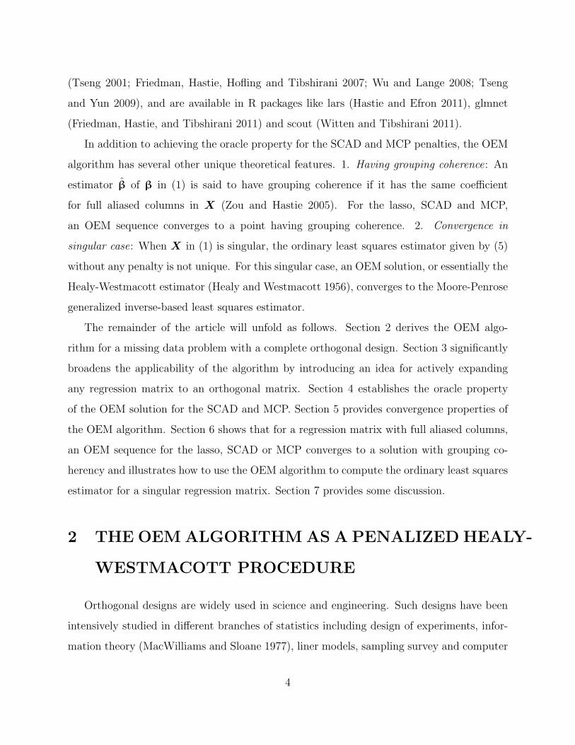
Example 6. We generate X from p dimensional Gaussian distribution N(0,V ) with n

independent observations, where the (i, j)th entry of V is 1 for i = j and ρ for i 6= j. Values

22

50 100 150 2000.65

0.7

0.75

0.8

0.85

0.9

0.95

n50 100 150 200

20

40

60

80

100

120

140

n

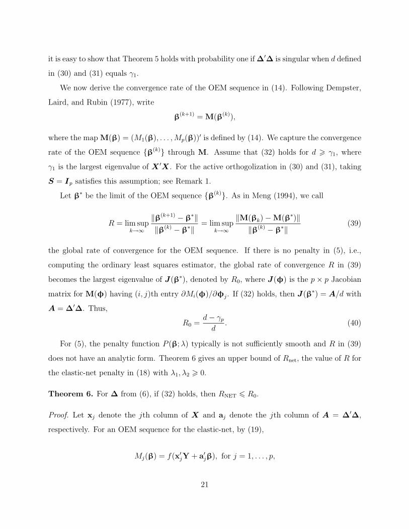
Figure 3. (Left) the average values of R0 in (40) against increasing n for Example 6; (right)the average iteration numbers against increasing n for Example 6, where the dashed andsolid lines denote the ordinary least squares estimator and the lasso, respectively.

of Y and β are generated by (1) and (22). The same setup was used in Friedman, Hastie,

and Tibshirani (2009). For p = 10, ρ = 0.1, λ = 0.5 and increasing n, the left panel of

Figure 3 depicts the average values of R0 in (40) against increasing n and the right panel of

the figure depicts the average iteration numbers against increasing n, with the dashed and

solid lines corresponding to the ordinary least squares estimator and the lasso, respectively.

Quite strikingly, this figure indicates that OEM requires fewer iterations as n becomes larger,

which makes OEM particulary attractive for situations with massive data (SAMSI 2012). It

is important to note that here the OEM sequence for the lasso requires fewer iteration than

its counterpart for the ordinary least squares, empirically validating Theorem 6.

6 POSSESSING GROUPING COHERENCE

In this section, we consider the convergence of the OEM algorithm when the regression

matrix X in (1) is singular due to fully aliased columns or other conditions. Let X be

standardized as in (4) with columns x1, . . . ,xp. If xi and xj are fully aliased, i.e., |xi| = |x2|,then the objective function in (5) for the lasso is not strictly convex and has many minima

(Zou and Hastie 2005). Data with fully aliasing structures commonly appear in observational

studies and various classes of experimental designs like supersaturated designs (Wu 1993;

Lin 1993; Tang and Wu 1997; Li and Lin 2002; Xu and Wu 2005) and factorial designs (Dey

23

and Mukerjee 1999; Mukerjee and Wu 2006).

Zou and Hastie (2005) states that if some columns of X are identical, it is desirable to

have grouping coherence by assigning the same coefficient to them. Definition 1 makes this

precise.

Definition 1. An estimator β = (β1, . . . , βp)′ of β in (1) has grouping coherence if xi = xj

implies βi = βj and xi = −xj implies βi = −βj.

Let 0p denote the zero vector in Rp. Let e+ij be the vector obtained by replacing the ith

and jth entries of 0p with 1. Let e−ij be the vector obtained by replacing the ith and jth

entries of 0p with 1 and −1, respectively. Let E denote the set of all e+ij and e−ij. By Definition

1, an estimator β has grouping coherence if and only if for any α ∈ E with Xα = 0, α′β = 0.

Lemma 2. Suppose that (32) holds. For the OEM sequence {β(k)} of the lasso, SCAD or

MCP, if Xα = 0 and α′β(k) = 0 for α ∈ E , then α′β(k+1) = 0.

Proof. For u defined in (10), we have that α′u = α′X ′Y + α′(dIp −X ′X)β(k) = 0 for any

α ∈ E with Xα = 0 and α′β(k) = 0. Then by (17), (12) and (21), an OEM sequence of the

lasso, SCAD or MCP satisfies the condition that if α′u = 0, then α′β(k+1) = 0 for α ∈ E .

This completes the proof.

Remark 7. Lemma 2 implies that, for k = 1, 2, . . ., β(k) has grouping coherence if β(0) has

grouping coherence. Thus, if {β(k)} converges, then its limit has grouping coherence. By

Theorem 5, if d > λ1 in (32), then an OEM sequence for the SCAD or MCP converges to a

point with grouping coherence.

When X in (1) has fully aliased columns, the objective function in (5) for the lasso

has many minima and hence the condition in Theorem 4 does not hold. Theorem 7 shows

that, even with full aliasing, an OEM sequence (17) for the lasso converges to a point with

grouping coherence.

Theorem 7. Suppose that (32) holds. If β(0) has grouping coherence, then as k →∞, the

OEM sequence {β(k)} of the lasso converges to a limit that has grouping coherence.

24

Proof. Partition the matrix X in (1) as (X1 X2), where no two columns of X2 are fully

aliased and any column of X1 is fully aliased with at least one column of X2. Let J

denote the number of columns in X1. Partition β as (β′1, β′2)′ and β(k) as (β

(k)′1 , β

(k)′2 )′,

corresponding to X1 and X2, respectively. For j = 1, . . . , p, let

ω(j) = #{i = 1, . . . , p : |xi| = |xj|}.

By Lemma 2, for j = 1, . . . , J , β(k)j = β

(k)j′ if xj = xj′ and β

(k)j = −β

(k)j′ otherwise, where

j′ ∈ {J + 1, . . . , p}. It follows that {β(k)2 } can be viewed as an OEM sequence for solving

minθ‖Y − Xθ‖2 + 2

p−J∑j=1

|θj|, (41)

where θ = (θ1, . . . , θp−J)′, and the columns of X are ω(J + 1)xJ+1, . . . , ω(p)xp. Because the

objective function in (41) is strictly convex, by Theorem 4, {β(k)2 } converges to a limit with

grouping coherence. This completes the proof.

Example 7. Consider X in Example 4. Let Y = (2, 1,−4, 1.5)′. Using an initial point

β(0) = 0, the OEM sequence of the lasso with λ = 1 converges to

β = (−0.5625, 0.4375, −0.6875, 0.6875, −0.4375, 0.5625)′,

which has grouping coherence. For the same data and the same initial point, the coordinate

descent sequence converges to 2(−0.5625, 0.4375, −0.6875, 0, 0, 0)′, which does not have

grouping coherence.

Theorem 7 shows that, if the initial point has grouping coherence, then every limit point

of the OEM sequence for the lasso inherits this property. It is now tempting to ask whether

such a result holds for the OEM sequence with λ = 0 in (16), i.e., the Healy and Westmacott

procedure. Since full aliasing is just one possible culprit for making the matrix X in (1) lack

full column rank and hence X ′X become singular, Theorem 8 provides an answer to this

question for the general singular situation.

25

Let r denote the rank of X. When r < p, the singular value decomposition (Wilkinson

1965) of X is

X = U ′

Γ

1/20 0

0 0

V ,

where U is an n× n matirx, V is a p× p orthogonal matrices and Γ0 is a diagonal matrix

whose diagonal elements are the positive eigenvalues, γ1 > · · · > γr, of X ′X. Define

β∗

= (X ′X)+X ′Y, (42)

where + denotes the Moore-Penrose generalized inverse (Ben-Israel and Greville 2003).

Theorem 8. Suppose that X ′X + ∆′∆ = γ1Ip. If β(0) lies in the linear space spanned by

the first r columns of V ′, then as k →∞, for the OEM sequence {β(k)} of the ordinary least

squares, β(k) → β∗.

Proof. Denote D = Ip − γ−11 X ′X. Note that β(k+1) = γ−1

1 X ′Y + Dβ(k). By induction,

β(k) = γ−11 (Ip + D + · · ·+ Dk−1)X ′Y + Dkβ(0)

= γ−11 V ′

Ip +

Ir − γ−1

1 Γ0 0

0 −Ip−r

+ · · ·+

(Ir − γ−1

1 Γ0)k−1 0

0 (−1)k−1Ip−r

V

·V ′

Γ

1/20 0

0 0

UY + Dkβ(0)

= γ−11 V ′

{Ir + (Ir − γ−1

1 Γ0) + · · ·+ (Ir − γ−11 Γ0)

k−1}Γ

1/20 0

0 0

UY + Dkβ(0).

As k →∞, we have that

Dk → V ′

0

Ip−r

V

26

and Dkβ(0) → 0, which implies that

β(k) → V ′

Γ

−1/20 0

0 0

UY = β

∗.

This completes the proof.

The condition X ′X + ∆′∆ = γ1Ip holds if S = Ip in (26).

Remark 8. Computing the Moore-Penrose generalized inverse β∗

in (42) is a difficult prob-

lem. Theorem 8 says that the OEM algorithm provides an efficient solution to this prob-

lem. When r < p, the limiting matrix β∗

given by an OEM sequence has the following

properties. First, it has the minimal Euclidean norm among the least squares estimators

(X ′X)−X ′Y (Ben-Israel and Greville 2003). Second, its model error has a simple form,

E[(β

∗ − β)′(X ′X)(β∗ − β)

]= rσ2. Third, Xα = 0 implies α′β

∗= 0 for any vector α,

which immediately implies that β∗

has grouping coherence.

Example 8. Use the same data and the same initial point in Example 7. The OEM sequence

of the ordinary least squares converges to

β∗

= (−0.6875, 0.5625, −0.8125, 0.8125, −0.5625, 0.6875)′,

which has grouping coherence.

7 DISCUSSION

For the regularized least squares method with the SCAD penalty, finding a local solu-

tion to achieve the oracle property is a well-known open problem. We have proposed an

algorithm, called the OEM algorithm, to fill this gap. For the SCAD and MCP penalties,

this algorithm can provide a local solution with the oracle property. The discovery of the

algorithm is quite accidental, drawing direct impetus from a missing-data problem arising in

design of experiments. The introduction of the active orthogonization procedure in Section 3

27

makes the algorithm applicable to very general data structures from observational studies

and experiments. Recent years have witnessed an explosive interest in both the theoretical

and computational aspects of penalized methods. Our introduction of an algorithm that not

only has desirable numerical convergence properties but also possesses an important theo-

retical property suggests a new interface between these two aspects. Subsequent work in

this direction is expected. The active orthogonization idea is general and may have potential

applications beyond the scope of the OEM algorithm, such as other EM algorithms (Meng

and Rubin 1991; Meng and Rubin 1993; Meng 2007), data augmentation (Tanner and Wong

1987), Markov chain Monte Carlo (Liu 2001), smoothing splines (Wahba and Luo 1997; Luo

1998), mesh-free methods in numerical analysis (Fasshauer 2007) and parallel computing

(Kumar, Grama, Gupta, and Karypis 2003). This procedure may also has intriguing math-

ematical connection with complementary theory in design of experiments (Tang and Wu

1996; Chen and Hedayat 1996; Xu and Wu 2005).

The result on the oracle property in Section 4 uses the assumption that the sample size n

goes to infinity. This result is appealing for practical situations with massive data (SAMSI

2012), such as the data deluge in astronomy, the Internet and marketing (the Economist

2010), large-scale industrial experiments (Xu 2009) and modern simulations in engineering

(NAE 2008), to just name a few. For applications like micro-array and image analysis, one

might be interested in extending the result to the small n and large p case, like in Fan and

Peng (2004). Such an extension, however, poses significant challenges. Even for a fixed p,

the penalized likelihood function for the SCAD can have a large number of local minima

(Huo and Chen 2010). When p goes to infinity, that number can be prohibitively large,

which makes it very difficult to sort out a local minima with the oracle property.

In addition to achieving the oracle property for nonconvex penalties, an OEM sequence

has other unique theoretical properties, including convergence to a point having grouping

coherence for the lasso, SCAD or MCP and convergence to the Moore-Penrose generalized

inverse-based least squares estimator for singular regression matrices. These theoretical

results together with the active orthogonization scheme form the main contribution of the

article.

28

A computer package for distributing the OEM algorithm to the general audience is under

development and will be released. We now remark on the acceleration issue and directions

for future work. The algorithm can be speeded up by using various methods from the EM

literature (McLachlan and Krishnan 2008). For example, following the idea in Varadhan and

Roland (2008), one can replace the OEM iteration in (14) by

β(k+1) = β(k) − 2γr + γ2v,

where r = M(β(k))−β(k), v = M(M(β(k)))−M(β(k))− r and γ = −‖r‖/‖v‖. This scheme

is found to lead to significant reduction of the running time in several examples. For problems

with very large p, one may consider a hybrid algorithm to combine the OEM and coordinate

descent ideas. It partitions β in (1) into G groups and in each iteration, it minimizes the

objective function l in (35) by using the OEM algorithm with respect to one group while

holding the other groups fixed. Here are some details. Group β as β = (β′1, . . . , β′G)′. For

k = 0, 1, . . ., solve

β(k+1)g = arg min

βg

l(β(k+1)1 , . . . , β

(k+1)g−1 , βg,β

(k)g+1, . . . , β

(k)G ) for g = 1, . . . , G (43)

by OEM until convergence. Note that (43) has a much lower dimension than the iteration

in (14). For G = 1, the hybrid algorithm reduces to the OEM algorithm and for G = p, it

becomes the coordinate descent algorithm. Theoretical properties of this hybrid algorithm

will be studied and reported elsewhere.

Extension of the OEM algorithm can be made by imposing special structures on regression

matrices, such as grouped variables (Yuan and Lin 2006; Zhou and Zhu 2008; Huang, Ma,

Xie, and Zhang 2009; Zhao, Rocha, and Yu 2009; Wang, Chen, and Li 2009; Xiong 2010),

mixtures (Khalili and Chen 2007) and heredity constraints (Yuan, Joseph, and Lin 2007;

Yuan, Joseph, and Zou 2009; Choi, Li, and Zhu 2010), among many other possibilities.

APPENDIX: PROOF OF THEOREM 1

29

Proof. We first give some definitions and notation. Let Φ be the cumulative distribution

function of the standard normal random variable. For a > 2 and λ in (3) and d > γ1 in

Assumption 1, define

s(u; λ) =

sign(u)(|u| − λ

)+/d, when |u| 6 (d + 1)λ,

sign(u){(a− 1)|u| − aλ

}/{(a− 1)d− 1

}, when (d + 1)λ < |u| 6 adλ,

u/d, when |u| > adλ,

Let s(u; λ) =[s(u1; λ), . . . , s(up; λ)

].′ The OEM sequence from (12) satisfies the condition

that β(k+1) = s(u(k); λn/n), where

u(k) = (u(k)′1 ,u

(k)′2 )′ =

X ′Yn

+

(dId − X ′Y

n

)β(k). (44)

For k = 1, 2, . . ., define two sequences of events Ak = {β(k)2 = 0} and Bk = {β(k)

1 =

u(k−1)1 /d}. For h > 0 and k = 0, 1, . . ., let Ch

k = {‖β(k)1 − β1‖ 6 hλn/n}. The flow of the

proof is to first show that P(Ak), P(Bk) and P(Chk ) all tend to one at exponential rates as n

goes to infinity, thus establishing Theorem 1 (i), then show that P(∩ki=1Ai) and P(∩k+1

i=1 Bi)

tend to one and finally establish Theorem 1(ii) by noting that the asymptotic normality of

β(k)1 follows when ∩k

i=1Ai and ∩k+1i=1 Bi both occur.

Step 1 . Let G = X(X ′X)−1 with columns g1, . . . ,gp. Let G1 denote its submatrix

with the first p1 columns. Let τ > 0 denote the largest eigenvalue of X ′1X2X

′2X1/n

2.

Define

hA =

1/(2τ), when τ > 0,

+∞, when τ = 0.(45)

Let (v1, . . . ,vp1) = dIp1 − n−1X ′1X1 and b = max{‖v1‖, . . . , ‖vp1‖}. Define

hB =ad

b, (46)

30

with a and d given in (3) and Assumption 1, respectively. For h > 0, define

hC =h

2η, (47)

where η, used in Assumption 3, is the largest eigenvalue of Ip1 −X ′1X1/(nd).

For Ch0 , since β(0) = β + G′ε, we have that

P(Ch0 ) = P(‖G′

1ε‖ 6 hλn/n)

> P(|g′jε| 6 hλn/(n

√p1) for j = 1, . . . .p1

)

> 1−p1∑

j=1

[1− P

(|g′jε| 6 hλn/(n√

p1))]

= 1− 2

p1∑j=1

[1− Φ

(hλn

n√

p1σ‖gj‖)]

. (48)

For A1, note that

P(A1) = P(|β(0)

j | 6 λn/(nd) for j = p1 + 1, . . . , p)

> 1−p∑

j=p1+1

[1− P

(|g′jε| 6 λn/(nd))]

= 1− 2

p∑j=p1+1

[1− Φ

(λn

ndσ‖gj‖)]

. (49)

For B1, note that

P(B1) = P(|β(0)

j | > aλn/n for j = 1, . . . , p1

)

> 1−p1∑

j=1

[1− P

(|βj + g′jε| > aλn/n)]

= 1−p1∑

j=1

[Φ

(nβj + aλn

nσ‖gj‖)− Φ

(nβj − aλn

nσ‖gj‖)]

. (50)

31

For any h > 0, by (48),

P(Ch1 ) > P(Ch

1 ∩B1) = P(Ch0 ∩B1)

> 1− 2

p1∑j=1

[1− Φ

(hλn

n√

p1σ‖gj‖)]

−p1∑

j=1

[Φ

(nβj + aλn

nσ‖gj‖)− Φ

(nβj − aλn

nσ‖gj‖)]

. (51)

Next, consider Ak, Bk and Chk , for k = 2, 3, . . .. If Ak−1 occurs, then by (44),

u(k−1) =X ′Xβ

n+

X ′εn

+

dIp1 −X ′

1X1/n −X ′1X2/n

−X ′2X1/n dIp−p1 −X ′

2X2/n

β

(k−1)1

0

.

Thus,

u(k−1)1 = dβ

(k−1)1 +

X ′1X1

n[β1 − β

(k−1)1 ] +

X ′1ε

n, (52)

u(k−1)2 =

X ′2X1

n[β1 − β

(k−1)1 ] +

X ′2ε

n. (53)

By (53),

P(Ak) > P(Ak ∩ Ak−1 ∩ ChAk−1)

= P({|u(k−1)

j | 6 λn/n for j = p1 + 1, . . . , p} ∩ Ak−1 ∩ ChAk−1

)

> P({‖u(k−1)

2 ‖ 6 λn/n} ∩ Ak−1 ∩ ChAk−1

)

= P({‖n−1X ′

2X1(β1 − β(k−1)1 ) + n−1X ′

2ε‖ 6 λn/n} ∩ Ak−1 ∩ ChAk−1

)

> P({‖n−1X ′

2ε‖ 6 λn/n− τ‖β1 − β(k−1)1 ‖} ∩ Ak−1 ∩ ChA

k−1

)

= P({‖n−1X ′

2ε‖ 6 λn/(2n)‖} ∩ Ak−1 ∩ ChAk−1

)

> P({|x′jε| 6 λn/(2

√p− p1) for j = p1 + 1, . . . , p} ∩ Ak−1 ∩ ChA

k−1

)

> 1− 2

p∑j=p1+1

[1− Φ

(λn

2√

p− p1σ‖xj‖)]

−[1− P(Ak−1)

]− [1− P(ChA

k−1)], (54)

32

where hA is defined in (45).

By (52),

P(Bk) > P(Bk ∩ Ak−1 ∩ ChBk−1)

= P({|dβj + u′j(β1 − β

(k−1)1 ) + n−1x′jε| > adλn/n for j = 1, . . . , p1} ∩ Ak−1 ∩ ChB

k−1

)

> P({|dβj + n−1x′jε| > |u′j(β1 − β

(k−1)1 )|+ adλn/n for j = 1, . . . , p1} ∩ Ak−1 ∩ ChB

k−1

)

> P({|dβj + n−1x′jε| > b‖β1 − β

(k−1)1 ‖+ adλn/n for j = 1, . . . , p1} ∩ Ak−1 ∩ ChB

k−1

)

> P({|dβj + n−1x′jε| > 2adλn/n for j = 1, . . . , p1} ∩ Ak−1 ∩ ChB

k−1

)

> 1−p1∑

j=1

[Φ

(ndβj + 2adλn

σ‖xj‖)− Φ

(ndβj − 2adλn

σ‖xj‖)]

− [1− P(Ak−1)

]

−[1− P(ChB

k−1)], (55)

where hB is defined in (46).

For any h > 0, we have that

P(Chk ) > P(Ch

k ∩Bk ∩ Ak−1 ∩ ChCk−1)

= P({‖(Ip1 −X ′

1X1/(nd))(β(k−1)1 − β1) + X ′

1ε/(nd)‖ 6 hλn/n} ∩Bk ∩ Ak−1 ∩ ChCk−1

)

> P({η‖β(k−1)

1 − β1‖+ ‖X ′1ε/(nd)‖ 6 hλn/n} ∩Bk ∩ Ak−1 ∩ ChC

k−1

)

> P({‖X ′

1ε/(nd)‖ 6 hλn/(2n)} ∩Bk ∩ Ak−1 ∩ ChCk−1

)

> P({|x′jε/(nd)| 6 hλn/(2n

√p1) for j = 1, . . . , p1} ∩Bk ∩ Ak−1 ∩ ChC

k−1

)

> 1− 2

p1∑j=1

[1− Φ

(hλn

2n√

p1σ‖xj‖)]

− [1− P(Ak−1)

]− [1− P(Bk)

]

−[1− P(ChC

k−1)], (56)

where hC is defined in (47).

33

Since 1− Φ(x) = o(exp(−x2/2)

)as x → +∞, (49), (50) and (51) imply that

1− P (A1) = o(exp[−c1(λn/

√n)2]

),

1− P (B1) = o(exp(−c2n)

)= o

(exp[−c2(λn/

√n)2]

),

1− P (Ch1 ) = o

(exp[−c3(λn/

√n)2]

),

where c1, c2 and c3 are positive constants. By induction, it now follows from (54), (55) and

(56) that

1− P (Ak) =[1− P (Ak−1)

]+

[1− P(ChA

k−1)]+ o

(exp[−c4(λn/

√n)2]

)

= o(k exp[−c4(λn/

√n)2]

), (57)

where c4 and c5 are positive constants. Similarly,

1− P (Bk) = o(k exp[−c6(λn/

√n)2]

), (58)

1− P (Chk ) = o

(k exp[−c7(λn/

√n)2]

), (59)

where c6 and c7 are positive constants. By (57), a sufficient condition for P(Ak) → 1 is

k exp[− c(λn/

√n)2

] → 0 (60)

for any c > 0, which is covered by Assumption 3.

Step 2 . Consider the asymptotic normality of β(k)1 . When the events Ak−1, Ak, Bk and

Bk+1 all occur, by (52),

X ′1X1

n(β

(k)1 − β1) =

X ′1ε

n+ d(β

(k)1 − β

(k+1)1 ), (61)

‖β(k+1)1 − β

(k)1 ‖ =

∥∥∥∥(

Ip1 −X ′

1X1

nd

)(β

(k)1 − β

(k−1)1 )

∥∥∥∥ 6 η‖β(k)1 − β

(k−1)1 ‖. (62)

34

When the events C1/21 , C

1/22 , A(k) =

⋂ki=1 Ai and B(k+1) =

⋂k+1i=1 Bi all occur, by (62),

‖β(k+1)1 − β

(k)1 ‖ 6 ηk−1‖β(2)

1 − β(1)1 ‖ 6 ηk−1λn/n. (63)

For any α ∈ Rp with α 6= 0, by (61) and (63),

|√nα′(β(k)1 − β1)−

√nα′(X ′

1X1)−1X ′

1ε|= dn3/2|α′(X ′

1X1)−1(β

(k)1 − β

(k+1)1 )|

6 n−1/2λnηk−1d‖α‖‖n(X ′1X1)

−1‖.

For any x ∈ R, note that

∣∣∣∣P(√

nα′(β(k)1 − β1) 6 x

)− Φ

(x

σ(α′Σ−11 α)1/2

)∣∣∣∣

6∣∣∣∣P

({√nα′(β(k)1 − β1) 6 x} ∩ C

1/21 ∩ C

1/22 ∩ A(k) ∩B(k+1)

)− Φ

(x

σ(α′Σ−11 α)1/2

)∣∣∣∣+

[1− P(C

1/21 )

]+

[1− P(C

1/21 )

]+

[1− P(A(k))

]+

[1− P(B(k+1))

]

6∣∣∣∣P

(√nα′(X ′

1X1)−1X ′

1ε 6 x− n−1/2λnηk−1d‖α‖‖n(X ′1X1)

−1‖)− Φ

(x

σ(α′Σ−11 α)1/2

)∣∣∣∣

+

∣∣∣∣P(√

nα′(X ′1X1)

−1X ′1ε 6 x + n−1/2λnηk−1d‖α‖‖n(X ′

1X1)−1‖)− Φ

(x

σ(α′Σ−11 α)1/2

)∣∣∣∣+3

[1− P(C

1/21 )

]+ 3

[1− P(C

1/21 )

]+ 3

[1− P(A(k))

]+ 3

[1− P(B(k+1))

]

=

∣∣∣∣Φ(

x− n−1/2λnηk−1d‖α‖‖n(X ′

1X1)−1‖

σ[α′n(X ′1X1)−1α]1/2

)− Φ

(x

σ(α′Σ−11 α)1/2

)∣∣∣∣

+

∣∣∣∣Φ(

x + n−1/2λnηk−1d‖α‖‖n(X ′

1X1)−1‖

σ[α′n(X ′1X1)−1α]1/2

)− Φ

(x

σ(α′Σ−11 α)1/2

)∣∣∣∣+6

[1− P(C

1/21 )

]+ 3

[1− P(A(k))

]+ 3

[1− P(B(k+1))

]. (64)

Now, under Assumption 3, by (57), (58) and (59), (64) converges to zero as n → ∞. This

completes the proof.

ACKNOWLEDGEMENTS

35

Xiong is supported by grant 10801130 of the National Natural Science Foundation of

China. Dai is partially support by Grace Wahba through NIH grant R01 EY009946, ONR

grant N00014-09-1-0655 and NSF grant DMS-0906818. Qian is partially supported by NSF

grant CMMI 0969616, an IBM Faculty Award and an NSF Faculty Early Career Development

Award DMS 1055214. The authors thank Xiao-Li Meng and Grace Wahba for comments

and suggestions.

REFERENCES

Addelman, S. (1962), “Orthogonal Main-Effect Plans for Asymmetrical Factorial Experi-

ments,” Technometrics, 4, 21-46.

Ben-Israel, A. and Greville, T. N. E. (2003), Generalized Inverses, Theory and Applications,

2nd ed., New York: Springer.

Bertsekas, D. P. (1999), Nonlinear Programming, 2nd ed., Belmont, MA: Athena Scientific.

Bingham, D., Sitter, R. R. and Tang, B. (2009). “Orthogonal and Nearly Orthogonal

Designs for Computer Experiments,” Biometrika, 96, 51–65.

Breiman, L. (1995), “Better Subset Regression Using the Nonnegative Garrote,” Techno-

metrics, 37, 373–384.

Breheny, P. and Huang, J. (2011), “Coordinate Descent Algorithms for Nonconvex Penal-

ized Regression, With Applications to Biological Feature Selection,” The Annals of

Applied Statistics, in press.

Chen, H. and Hedayat, A. S. (1996), “2n−l designs with Weak Minimum Aberration,” The

Annals of Statistics, 24, 2536–2548.

Choi, N. H., Li W. and Zhu J. (2010), “Variable Selection With the Strong Heredity Con-

straint and Its Oracle Property,” Journal of the American Statistical Association, 105,

354–364.

36

Dempster, A. P., Laird, N. M. and Rubin, D. B. (1977), “Maximum Likelihood from In-

complete Data via the EM Algorithm,” Journal of the Royal Statistical Society, Ser.

B, 39, 1–38.

Deng, X., Lin, C. D. and Qian, P. Z. G. (2010), “Designs for the Lasso,” Technical Report.

Dey, A. and Mukerjee, R. (1999), Fractional Factorial Plans, New York: Wiley.

Efron, B., Hastie, T., Johnstone, I. and Tibshirani, R. (2004), “Least Angle Regression,”

The Annals of Statistics, 32, 407–451.

Fan, J. and Li, R. (2001), “Variable Selection via Nonconcave Penalized Likelihood and Its

Oracle Properties,” Journal of the American Statistical Association, 96, 1348–1360.

Fan, J. and Peng, H. (2004), “On Non-concave Penalized Likelihood With Diverging Num-

ber of Parameters,” The Annals of Statistics, 32, 928–961.

Fang, K. T., Li, R. and Sudjianto, A. (2005), Design and Modeling for Computer Experi-

ments, New York: Chapman and Hall/CRC Press.

Fasshauer, G. F. (2007), Meshfree Approximation Methods With MATLAB, Singapore:

World Scientific Publishing Company.

Frank, L. E. and Friedman, J. (1993), “A Statistical View of Some Chemometrics Regression

Tools,” Technometrics, 35, 109–135.

Friedman, J., Hastie, T., Hofling, H. and Tibshirani, R. (2007), “Pathwise Coordinate

Optimization,” The Annals of Applied Statistics, 1, 302–332.

Friedman, J., Hastie, T. and Tibshirani, R. (2009), “Regularization Paths for Generalized

Linear Models via Coordinate Descent,” Journal of Statistical Software, 33, 1–22.

Friedman, J., Hastie, T. and Tibshirani, R. (2011), “Glmnet,” R package.

Fu, W. J. (1998), “Penalized Regressions: The Bridge versus the LASSO,” Journal of

Computational and Graphical Statistics, 7, 397–416.

37

Grandvalet, Y. (1998), “Least Absolute Shrinkage Is Equivalent to Quadratic Penalization,”

In: Niklasson, L., Boden, M., Ziemske, T. (eds.), ICANN’98. Vol. 1 of Perspectives

in Neural Computing, Springer, 201–206.

Green, P. J. (1990), “On Use of the EM Algorithm for Penalized Likelihood Estimation,”

Journal of the Royal Statistical Society, Ser. B, 52, 443–452.

Hastie, T. and Efron, B. (2011), “Lars,” R package.

Healy, M. J. R. and Westmacott, M. H. (1956), “Missing Values in Experiments Analysed

on Automatic Computers,” Journal of the Royal Statistical Society, Ser. C, 5, 203–206.

Hedayat, A. S., Sloane, N. J. A. and Stufken, J. (1999), Orthogonal Arrays: Theory and

Applications, New York: Springer.

Hoerl, A. E. and Kennard, R. W. (1970), “Ridge Regression: Biased Estimation for

Nonorthogonal Problems,” Technometrics, 12, 55–67.

Huang, J., Ma, S., Xie, H. and Zhang, C-H. (2009), “A Group Bridge Approach for Variable

Selection,” Biometrika, 96, 339–355.

Hunter, D. R. and Li, R. (2005), “Variable Selection Using MM Algorithms,” The Annals

of Statistics, 33, 1617–1642.

Huo, X. and Chen, J. (2010), “Complexity of Penalized Likelihood Estimation,” Journal of

Statistical Computation and Simulation, 80, 747–759 .

Huo, X. and Ni, X. L. (2007), “When Do Stepwise Algorithms Meet Subset Selection

Criteria?” The Annals of Statistics, 35, 870–887.

Khalili, A. and Chen, J. (2007), “Variable Selection in Finite Mixture of Regression Mod-

els,” Journal of the American Statistical Association, 102, 1025–1038.

Kumar, V., Grama, A., Gupta, A. and Karypis, G. (2003), Introduction to Parallel Com-

puting, 2nd ed., Boston, MA: Addison Wesley.

38

Lin, C. D., Bingham, D., Sitter, R. R. and Tang, B. (2010), “A New and Flexible Method

for Constructing Designs for Computer Experiments,” The Annals of Statistics, 38,

1460–1477.

Lin, C. D., Mukerjee, R. and Tang, B. (2009), “Construction of Orthogonal and Nearly

Orthogonal Latin Hypercubes,” Biometrika, 96, 243–247.

Li, R. and Lin, D. K. J. (2002), “Data Analysis in Supersaturated Designs,” Statistics and

Probability Letters, 59, 135–144.

Lin, D. K. J. (1993), “A New Class of Supersaturated Designs,” Technometrics, 35, 28–31.

Liu, J. S. (2001), Monte Carlo Strategies in Scientific Computing, New York: Springer.

Luo, Z. (1998), “Backfitting in Smoothing Spline ANOVA,” The Annals of Statistics, 26,

1733–1759.

MacWilliams, F. J. and Sloane, N. J. A. (1977), The Theory of Error Correcting Codes,

New York: North-Holland.

Mazumder, R., Friedman, J. and Hastie, T. (2010), “SparseNet: Coordinate Descent with

Non-Convex Penalties,” Technical Report.

McLachlan, G. and Krishnan, T. (2008), The EM Algotithm and Extensions, 2nd ed., New

York: Wiley.

Meng, X. L. (1994), “On the Rate of Convergence of the ECM Algorithm,” The Annals of

Statistics, 22, 326–339.

Meng, X. L. (2007), “Thirty Years of EM and Much More,” Statistica Sinica, 17, 839–840.

Meng, X. L. and Rubin, D. (1991), “Using EM to Obtain Asymptotic Variance-Covariance

Matrices: The SEM Algorithm,” Journal of the American Statistical Association, 86,

899–909.

39

Meng, X. L. and Rubin, D. (1993), “Maximum Likelihood Estimation via the ECM Algo-

rithm: A General Framework,” Biometrika, 80, 267–278.

Mukerjee, R. and Wu, C. F. J. (2006), A Modern Theory of Factorial Design, New York:

Springer.

NAE (2008), “Grand Challenges for Engineering,” Technical report, The National Academy

of Engineering.

Nettleton, D. (1999), “Convergence Properties of the EM Algorithm in Constrained Pa-

rameter Spaces,” Canadian Journal of Statistics, 27, 639–648.

Osborne, M. R., Presnell, B. and Turlach, B. (2000), “On the LASSO and Its Dual,” Journal

of Computational and Graphical Statistics, 9, 319–337.

Owen, A. B. (1994), “Controlling Correlations in Latin Hypercube Samples,” Journal of

the American Statistical Association, 89, 1517–1522.

Owen, A. B. (2006), “A Robust Hybrid of Lasso and Ridge Regression,” Technical Report.

Pang, F., Liu, M. Q. and Lin, D. K. J. (2009), “A Construction Method for Orthogonal

Latin Hypercube Designs with Prime Power Levels,” Statistica Sinica, 19, 1721–1728.

Phoa, F. K. H., Pan, Y-H. and Xu, H. (2009), “Analysis of Supersaturated Designs via The

Dantzig Selector,” Journal of Statistical Planning and Inference, 139, 2362–2372.

Rubin, D. B. and Szatrowski, T. H. (1982), “Finding Maximum Likelihood Estimates of

Patterned Covariance Matrices by the EM Algorithm,” Biometrika, 69, 657–660.

SAMSI (2012), Program on Statistical and Computational Methodology for Massive Datasets,

2012-2013.

Santner, T. J., Williams, B. J. and Notz, W. I. (2003), The Design and Analysis of Computer

Experiments, New York: Springer.

40

Schifano, E. D., Strawderman, R. and Wells, M. T. (2010), “Majorization-Minimization

Algorithms for Nonsmoothly Penalized Objective Functions,” Electronic Journal of

Statistics, 23, 1258–1299.

Steinberg, D. M. and Lin, D. K. J. (2006), “A Construction Method for Orthogonal Lain

Hypercube Designs,” Biometrika, 93, 279–288.

Sun, F., Liu, M. and Lin, D. K. J. (2009), “Construction of Orthogonal Latin Hypercube

Designs,” Biometrika, 96, 971–974.

Tang, B. (1998), “Selecting Latin Hypercubes Using Correlation Criteria,” Statistica Sinica,

8, 965–977.

Tang, B. and Wu, C. F. J. (1996), “Characterization of Minimum Aberration 2n−k Designs

in terms of Their Complementary Designs,” The Annals of Statistics, 24, 2549–2559.

Tang, B. and Wu, C. F. J. (1997), “A Method for Constructing Supersaturated Designs

and Its E(s2) Optimality,” Canadian Journal of Statistics, 25, 191–201.

Tanner, M. A. and Wong, W. H. (1987). “The Calculation of Posterior Distributions by

Data Augmentation,” Journal of the American Statistical Association, 82, 528–540.

The Economist (2010), “Special Report on the Data Deluge, (February 27),” The Economist,

394, 3–18.

Tibshirani, R. (1996), “Regression Shrinkage and Selection via the Lasso,” Journal of the

Royal Statistical Society, Ser. B, 58, 267–288.

Tseng, P. (2001), “Convergence of a Block Coordnate Descent Method for Nondifferentialble

Minimization,” Journal of Optimization Theory and Applications, 109, 475–494.

Tseng, P. and Yun, S. (2009), “A Coordinate Gradient Descent Method for Nonsmooth

Separable Minimization,” Mathematical Programming B, 117, 387–423.

41

Varadhan, R. and Roland, C. (2008), “Simple and Globally Convergent Methods for Accel-

erating the Convergence of Any EM Algorithm,” Scandinavian Journal of Statistics,

35, 335–353.

Wahba, G. and Luo, Z. (1997), “Smoothing Spline ANOVA Fits for Very Large, Nearly

Regular Data Sets, with Application to Historical Global Climate Data,” Annals of

Numerical Mathematics, 4579-4598. (Festschrift in Honor of Ted Rivlin, C. Micchelli,

Ed.)

Wang, L., Chen, G. and Li, H. (2007), “Group SCAD Regression Analysis for Microarray

Time Course Gene Expression Data,” Bioinformatics, 23, 1486–1494.

Watkins, D. S. (2002), Fundamentals of Matrix Computations, 2nd ed., New York: Wiley.

Wilkinson, J. H. (1965), The Algebraic Eigenvalue Problem, New York: Oxford University

Press.

Witten, D. M. and Tibshirani, R. (2011), “Scout,” R package.

Wu, C. F. J. (1983), “On the Convergence Properties of the EM Algorithm,” The Annals

of Statistics, 11, 95–103.

Wu, C. F. J. (1993), “Construction of Supersaturated Designs through Partially Aliased

Interactions,” Biometrika, 80, 661–669.

Wu, C. F. J. and Hamada M. (2009), Experiments: Planning, Analysis, and Optimization,

2nd ed., New York: Wiley.

Wu, T. and Lange, K. (2008), “Coordinate Descent Algorithm for Lasso Penalized Regres-

sion,” The Annals of Applied Statistics, 2, 224–244.

Xiong, S. (2010), “Some Notes on the Nonnegative Garrote,” Technometrics, 52, 349–361.

Xu, H. (2009), “Algorithmic Construction of Efficient Fractional Factorial Designs With

Large Run Sizes,” Technometrics, 51, 262–277.

42

Xu, H. and Cheng, C-S. (2008), “A Complementary Design Theory for Doubling,” The

Annals of Statistics, 36, 445–457.

Xu, H. and Wu, C. F. J. (2005), “Construction of Optimal Multi-Level Supersaturated

Designs,” The Annals of Statistics, 33, 2811–2836.

Ye, K. Q. (1998). “Orthogonal Column Latin Hypercubes and Their Applications in Com-

puter Experiments,” Journal of the American Statistical Association, 93, 1430–1439.

Yuan, M. and Lin, Y. (2006), “Model Selection and Estimation in Regression with Grouped

Variables,” Journal of the Royal Statistical Society, Ser. B, 68, 49–68.

Yuan, M., Joseph, V. R. and Lin, Y. (2007), “An Efficient Variable Selection Approach for

Analyzing Designed Experiments,” Technometrics, 49, 430–439.

Yuan, M., Joseph, V. R. and Zou, H. (2009), “Structured Variable Selection and Estima-

tion,” Annals of Applied Statistics, 3, 1738–1757.

Zangwill, W. I. (1969), Nonlinear Programming: A Unified Approach, Englewood Cliffs,

New Jersey: Prentice Hall.

Zhang. C-H. (2010), “Nearly Unbiased Variable Selection under Minimax Concave Penalty,”

The Annals of Statistics, 38, 894–942.

Zhao, P., Rocha, G. and Yu, B. (2009), “The Composite Absolute Penalties Family for

Grouped and Hierarchical Variable Selection,” The Annals of Statistics, 37, 3468–3497.

Zhou, N. and Zhu, J. (2008), “Group Variable Selection via a Hierarchical Lasso and Its

Oracle Property,” Technical Report.

Zhu, Y. (2011), Personal communication.

Zou, H. and Hastie, T. (2005), “Regularization and Variable Selection via the Elastic Net,”

Journal of the Royal Statistical Society, Ser. B, 67, 301–320.

43

Zou, H. and Li, R. (2008), “One-step Sparse Estimates in Nonconcave Penalized Likelihood

Models,” The Annals of Statistics, 36, 1509–1533.

44