ORTHOGONAL PRINCIPAL PLANES

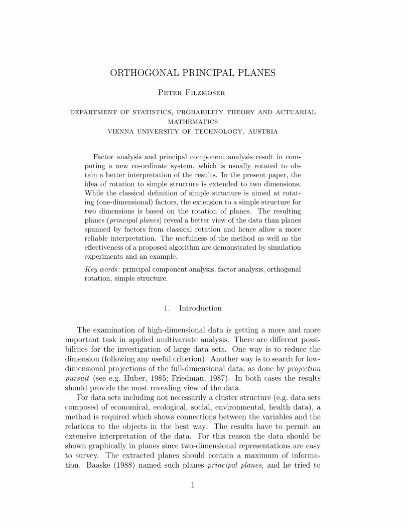
ORTHOGONAL PRINCIPAL PLANES

Peter Filzmoser

department of statistics, probability theory and actuarialmathematics

vienna university of technology, austria

Factor analysis and principal component analysis result in com-puting a new co-ordinate system, which is usually rotated to ob-tain a better interpretation of the results. In the present paper, theidea of rotation to simple structure is extended to two dimensions.While the classical definition of simple structure is aimed at rotat-ing (one-dimensional) factors, the extension to a simple structure fortwo dimensions is based on the rotation of planes. The resultingplanes (principal planes) reveal a better view of the data than planesspanned by factors from classical rotation and hence allow a morereliable interpretation. The usefulness of the method as well as theeffectiveness of a proposed algorithm are demonstrated by simulationexperiments and an example.

Key words: principal component analysis, factor analysis, orthogonalrotation, simple structure.

1. Introduction

The examination of high-dimensional data is getting a more and moreimportant task in applied multivariate analysis. There are different possi-bilities for the investigation of large data sets. One way is to reduce thedimension (following any useful criterion). Another way is to search for low-dimensional projections of the full-dimensional data, as done by projectionpursuit (see e.g. Huber, 1985; Friedman, 1987). In both cases the resultsshould provide the most revealing view of the data.

For data sets including not necessarily a cluster structure (e.g. data setscomposed of economical, ecological, social, environmental, health data), amethod is required which shows connections between the variables and therelations to the objects in the best way. The results have to permit anextensive interpretation of the data. For this reason the data should beshown graphically in planes since two-dimensional representations are easyto survey. The extracted planes should contain a maximum of informa-tion. Baaske (1988) named such planes principal planes, and he tried to

1

find triplets of variables spanning a plane which should represent the othervariables as good as possible.

The present paper gives another approach for obtaining principal planes.At the basis of a decomposition of the (standardized) data matrix by factoranalysis or principal component analysis, the matrix of loadings is rotated toa simple structure for planes. This is a generalization to higher dimensionsof the classical simple structure introduced by Thurstone (1944). One couldextend these thoughts also to higher dimensions; we would then considerprincipal spaces.

Classical rotation methods extract (one-dimensional) factors which shouldcharacterize all variables in a good fashion, and at the same time differentfactors should include different variables. This provides the factors to beinterpreted as non observable quantities, where each factor characterizesother properties. The results are mostly presented by plots where eachfactor is drawn against another one. Unfortunately, these planes are notconstructed to be most meaningful, since by ideal simple structure the vari-ables are close to the axes. The contents of information of a resulting planecould be increased by directly extracting planes instead of vectors (factors).

For rotation to principal planes, two-dimensional factors (pairs of factorsspanning a plane) with the same properties as formulated above are to befound. All variables should be well presented by the principal planes, andeach principal plane should characterize other variables. This constructionenables a configuration, where the variables are close to the principal plane(spanned by two factors), and not just close to the axes. As a consequence,in general more variables are well presented by the resulting plane, andtherefore the interpretation of the results can be more extensive and shouldbe more reliable.

This paper is organized as follows: In section 2 basic considerationsabout simple structure for planes are given. Moreover, the classical varimax-criterion (Kaiser, 1958), in the following abbreviated by VMAX, is extendedto a varimax-criterion for planes (VMAX2). Section 3 is concerned with analgorithm for VMAX2. The rotation is based on an iterative procedure.The criterion is improved step-by-step, until no essential change of the so-lution is visible. Since no explicit solution of the optimization criterionexists, an approximation has to be found in each step of the iteration. Theperformance of the algorithm is demonstrated by simulation experiments insection 4. Section 5 shows the application of the procedure to a real dataset.

2

2. Method

Basis for rotation to principal planes is the unrotated matrix of load-ings obtained by factor analysis or principal component analysis. Let Λdenote the given (p × k) orthogonal pattern, and let f = (f1, . . . , fk)>

be the standardized factors arising by linear transformation of the origi-nal standardized variables y = (y1, . . . , yp)> with the coefficients Λ, i.e.y = Λf + e. In more detail, the (i, j)-th element of Λ, λij, represents theconnection between variable yi and factor fj, and this relation is used forobtaining classical simple structure: High loadings for a variable on one fac-tor should occur, while at the same time the loadings on the other factorsshould be low. For the well known and frequently used varimax-criterion(Kaiser, 1958), the simple structure is realized by maximizing the sum overthe variances of the squared (standardized) factor loadings for each factor,i.e.

1p

k∑

j=1

p∑

i=1

( ˜λij

κi

)4− 1

p2

k∑

j=1

[p

∑

i=1

( ˜λij

κi

)2]2= max . (1)

˜λij is an element of the rotated matrix of loadings, and κ2i =

∑kj=1 λ2

ij(i = 1, . . . , p) is called i-th communality. It describes the proportion ofvariance of the i-th standardized variable explained by all k factors. Thecommunalities are used for standardization to avoid large influence of vari-ables with high communalities.

Simple structure for planes also uses the relationship between variablesand planes, expressed by the multiple correlation. Explicitly, for a vari-able yi (i = 1, . . . , p) and a plane spanned by two different factors fa

and fb (a, b = 1, . . . , k; a 6= b), the multiple correlation between yi andf = (fa, fb)> is defined by

ρyi;f = (ρ>fyiρ−1

ffρfyi)1/2 (2)

(see e.g. Mardia et al., 1979) where ρfyiis a (2× 1)-matrix with the corre-

lations between factors and the variable at hand, and ρff is the correlationmatrix of the factors fa and fb. If the factors are supposed to be orthogonal,ρff (and therefore ρ−1

ff ) is the identity. The correlations between yi andthe factors in the orthogonal case are exactly the loadings, so the aboveequation reduces to

ρyi;f =√

λ2ia + λ2

ib . (3)

To simplify the notation, the multiple correlation between yi and f =(fa, fb)> is denoted by ρi;a,b.

3

A next point for developing a rotation criterion for planes is to definemore precisely how the planes are constructed. The aim is to obtain planesspanned by different and disjoint pairs of factors. If the number of factors, k,is even, q = k/2 pairs of factors are forming the planes. For an odd numberk, one factor is omitted and the results are q = (k − 1)/2 planes. Each setof pairs can be defined by simply ordering the k factors in a particular way(calling the first two factors the first pair, the second two the second pair,etc.). Hence, there are k! such sets of pairs. However, among these k! sets ofpairs many are essentially the same: First of all, all pairs appear twice (as(a, b) and (b, a)), hence, to correct for this, the number k! has to be dividedby 2 for each pair, hence by 2q for the q pairs. Furthermore, sets of q pairsthat only differ with respect to the order in which the pairs are given areequal, hence the result has to be divided by q!, the number of permutationsin which the pairs can occur. This gives a total number of combinations ofdifferent planes with disjoint factors of

E =k!

2qq!. (4)

Let sl (l = 1, . . . , E) denote the indices of the factors for one particularcombination of planes, and let S = {sl | l = 1, . . . , E} be the set of thesecombinations. E.g. for k = 6 factors, one element of S might be the set{(1, 2), (3, 4), (5, 6)}.

A rotation criterion for simple structure for planes has to find the opti-mum over all E combinations of planes, i.e. the best result over all factorcombinations s ∈ S. The simplicity of the structure is defined at the basisof the relation between variables and planes, given by (2) or, for orthogonalfactors, by (3). Similar to the classical case, this value should be high for avariable at one plane and at the same time low at the other planes.

With this knowledge the ideas of VMAX (1) can be easily extendedto a varimax-criterion for planes. The simple structure for planes can berealized by considering the variance of the squared “loadings on the planes”which are defined by (2). If the planes are spanned by the factors {fa, fb}({(a, b)} ∈ s), this variance is

s2a,b =

1p

p∑

i=1

(

ρ2i;a,b

)2− 1

p2

[ p∑

i=1ρ2

i;a,b

]2

(5)

or, since the factors are supposed to be orthogonal,

s2a,b =

1p

p∑

i=1

(

˜λ2ia + ˜λ2

ib

)2− 1

p2

[ p∑

i=1

(

˜λ2ia + ˜λ2

ib

)

]2

(6)

4

where ρ2i;a,b = ˜λ2

ia + ˜λ2ib. Equation (6) describes the variance of the squared

multiple correlations (SMC) of the variables yi with the plane {fa, fb}. Inanalogy to VMAX, the variances given by (6) have to be summarized overall planes of a combination s, and the loadings are to be divided by thecorresponding communalities. The resulting expression has to be maximizedby an orthogonal transformation. Finally, the maximum over all differentcombinations s ∈ S has to be found. Expressed by a formula, the varimax-criterion for planes is defined by

V MAX2 = maxs∈S

∑

{(a,b)}∈s

pp

∑

i=1

( ρi;a,b

κi

)4

−( p

∑

i=1

( ρi;a,b

κi

)2)2

= max

.

(7)The results are principal planes spanned by the factors {fa, fb} ({(a, b)} ∈s). Note that criterion (7) can easily be modified to obtain a two-dimensionalextension of the quartimax-criterion (Carroll, 1953), the quartimax-criterionfor planes:

QMAX2 = maxs∈S

∑

{(a,b)}∈s

p∑

i=1

( ρi;a,b

κi

)4

= max

. (8)

3. Algorithm

A numerical solution of the varimax-criterion for planes can be foundby an iterative process. In each iteration two different planes spanned bythe factors {fa, fb} and {fc, fd} ({(a, b), (c, d)} ∈ s, a 6= c), respectively, areconsidered. In this 4-dimensional space the varimax-criterion for the twoplanes is defined by

V MAX2a,b;c,d = pp

∑

i=1

[

( ρi;a,b

κi

)4+

( ρi;c,d

κi

)4]

−[ p∑

i=1

( ρi;a,b

κi

)2]2

−[ p∑

i=1

( ρi;c,d

κi

)2]2

. (9)

Since an orthogonal rotation in 4 dimensions would be rather complicated,the rotation is performed in 4 steps in the planes {fa, fc}, {fb, fd}, {fa, fd}and {fb, fc}. Steps 1-4 are repeated until (9) cannot be further increased.If this is done, the four steps are applied to another two planes of the com-bination s, and so on. The entire process is started again until convergence,

5

this means until the varimax-criterion for planes (7) cannot be further im-proved. In order to avoid that the algorithm converges to a local maximum,several orthogonal random starts of the whole procedure have to be done(see also Gebhardt, 1968; ten Berge, 1984). More information about thepractical performance of this procedure is given in the next section.

Let us consider the optimization in one particular plane, say, in the planespanned by the factors {fa, fc}, in more detail. The rotated loadings arecomputed by the orthogonal transformation

˜λia = λia cos ϑ + λic sin ϑ (10)˜λic = −λia sin ϑ + λic cos ϑ (11)˜λij = λij for j 6= a, c (12)

and i = 1, . . . , p. The rotation angle in this plane is ϑ. Insertion of therotated loadings into (9) gives

V MAX2a,b;c,d = pp

∑

i=1

[

[(λia cos ϑ + λic sin ϑ)2 + λ2ib]

2

κ4i

+[(−λia sin ϑ + λic cos ϑ)2 + λ2

id]2

κ4i

]

−[ p∑

i=1

(λia cos ϑ + λic sin ϑ)2 + λ2ib

κ2i

]2

−[ p∑

i=1

(−λia sin ϑ + λic cos ϑ)2 + λ2id

κ2i

]2

. (13)

Two indices are underlined in the above formula to indicate, in which planethe rotation is performed. For maximizing (13), the first derivative withrespect to ϑ is calculated and the result is set equal to zero. Since thisderivative has no explicit solution for the parameter ϑ, an approximationcan be found for example by the regula-falsi method (see e.g. Golub andOrtega, 1993) described below.

Equation (13) may be rewritten in the form

f(ϑ) = c1 sin(4ϑ) + c2 cos(4ϑ) + c3 sin(2ϑ) + c4 cos(2ϑ) + c5 (14)

where c1 to c5 are constants depending on the loadings. In general, theperiodicity of the function f is π. This means that for finding the maximumone is interested in a rotation of the factors within the interval (−π

2 , π2 ). The

maximum can be found approximately by performing the following steps:

Step 1: Select P fixed regularly distributed values ϑ1, . . . , ϑP within the inter-val [−π

2 , π2 ] and compute the function values f(ϑ1), . . . , f(ϑP ).

6

Step 2: Search for the maximum f(ϑm) of the P function values and take theneighbors of ϑm, which are ϑm−1 and ϑm+1. For m = 1 the neighborsare −π

2 and ϑ2, for m = P take ϑP−1 and π2 .

Step 3: Compute the values f ′(ϑm−1) and f ′(ϑm+1), which are the starting val-ues for the regula falsi method. Since f is continuous, sgnf ′(ϑm−1) 6=sgnf ′(ϑm+1) if P is large enough.

Step 4: Compute the zero point ϑz of the connection line between f ′(ϑm−1)and f ′(ϑm+1) by

ϑz = ϑm−1 − f ′(ϑm−1)ϑm+1 − ϑm−1

f ′(ϑm+1)− f ′(ϑm−1). (15)

Step 5: If f ′(ϑz) = 0 (or ≈ 0), a real zero of f ′ within the interval (−π2 , π

2 ) hasbeen found. In the other case sgnf ′(ϑz) 6= sgnf ′(ϑm−1) or sgnf ′(ϑz) 6=sgnf ′(ϑm+1), and the procedure can be started with the correspondingnew interval from step 4 .

Figure 1 illustrates the proposed procedure. For P = 10 fixed points(which would be too small in practice) the function values are computed.After performing the regula falsi method, the first approximation of themaximum of f at ϑz is obtained. The second approximation is already veryclose to the real maximum.

Increasing P implies a longer computation time for one iteration of theregula-falsi method. On the other hand, the number of iterations in generaldecreases since the maximum f(ϑm) for larger P (step 2) will in generalbe closer to the final maximum. It turned out in practice that a choice ofP = 50 is a good compromise.

A computer program with the proposed algorithm in the language GAUSScan be obtained from the author.

Figure 1 is inserted about here.

4. Simulation

The proposed rotation method is tested in the following by simulationexperiments. A matrix of loadings with p = 100 variables and k = 4 factorsis generated randomly. The first 50 variables have two nonzero loadings

7

at the first two factors, the last 50 variables have two nonzero loadings atthe last two factors, i.e. the target pattern has complexity 2. The nonzeroloadings are uniformly distributed in the interval [−1, 1]. For each variable,the loadings are standardized by their communality.

The simulated pattern is scrambled in each of 50 replications by ran-dom orthogonal rotations, and the rotation methods quartimax and vari-max (classically and for planes) are applied. For each analysis the iterativeprocess was considered to have converged if the relative difference of theobjective function of two consecutive cycles was below 10−6. The conver-gence was reached in each of the following simulations already after a fewiterations.

The resulting rotated loadings are compared with the original ones bypermuting and reflecting the columns to obtain optimal congruence with thetruly simple pattern. For each row of the loading matrices, the Euclideannorm of the difference to the corresponding row of the truly simple patternwas computed. The mean of these values has been taken as a measure ofgoodness of recovering the original pattern. Expressed by a formula, thismeasure which is called congruence index is defined by

C =1p

p∑

i=1

k∑

j=1

(

λij −k

∑

l=1

ailtlj

)2

1/2

(16)

where λij is the (i, j)-th element of the target pattern, ail is the (i, l)-thelement of the randomly rotated pattern, and tlj is the (l, j)-th element ofthe best transformation matrix obtained by each rotation method at hand.

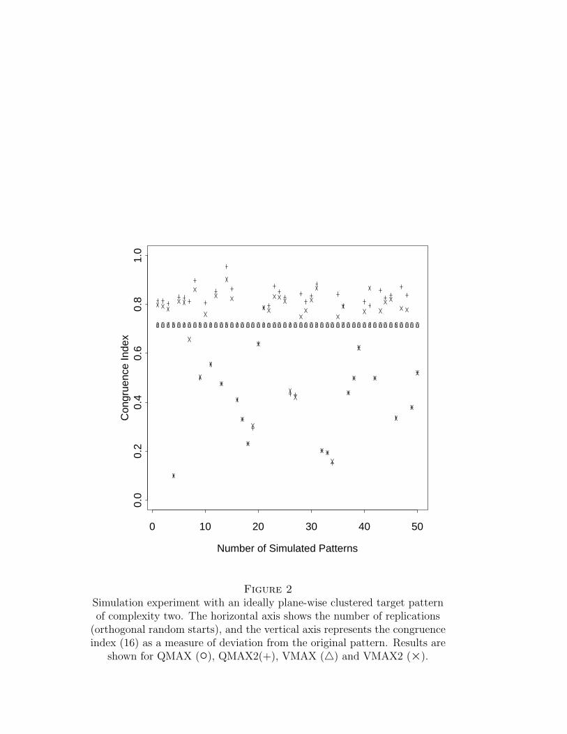
The result of this study is shown in Figure 2. The horizontal axis showsthe number of replications of the simulation, the vertical axis represents thecongruence index (16) as the measure of deviation from the original pattern.The results of QMAX are labeled by ◦, those of QMAX2 by +, VMAX by4, and VMAX2 by ×.

Since no noise has been added to the target pattern, and since the pat-tern is ideally plane-wise clustered, a congruence index of 0 would indicatethe best solution (global minimum). Figure 2 shows that the results for theclassical rotation methods QMAX and VMAX do not change by orthogo-nally rotating the target. Moreover, these methods lead to the same results(up to the given precision of the optimization procedure of the algorithm).QMAX2 and VMAX2 are strongly depending on orthogonal random starts.About half of the solutions of the rotation methods for planes are better thanthe classical methods, some are much better. It is interesting that VMAX2and QMAX2 give about the same result if the solution comes closer to theglobal optimum; otherwise VMAX2 is slightly better than QMAX2.

8


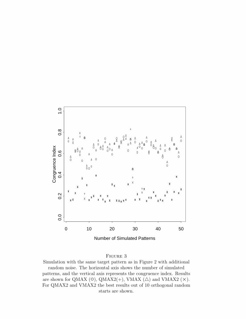
The second simulation experiment uses the same target pattern as be-fore. This pattern is contaminated in each of 50 simulations with randomnoise, the elements of which are distributed according to N(0, 1/10). Thesimulated patterns are scrambled by random orthogonal rotations and thesame rotation methods as in the previous experiment are used for patternrecovery. Since QMAX2 and VMAX2 are sensitive to local optima, 10randomized starting positions are chosen by orthogonal random rotationsof each simulated pattern, and the best solution is taken as the best ap-proximation of the global optimum. The result of this study is presentedin Figure 3 where the number of replications of the simulation is drawnagainst the congruence index (16). A big difference between the classicalmethods and rotation methods for planes is visible. Just for 2 out of 50simulations the classical methods lead to better results. QMAX gives ingeneral a lower value of the congruence index than VMAX. Like in the pre-vious experiment, the results of QMAX2 and VMAX2 are very similar. Itis interesting to compute the average of the congruence indices over all 50simulations. The value for QMAX is 0.64, VMAX gives 0.66, QMAX2 andVMAX2 are much lower with a value of 0.24.


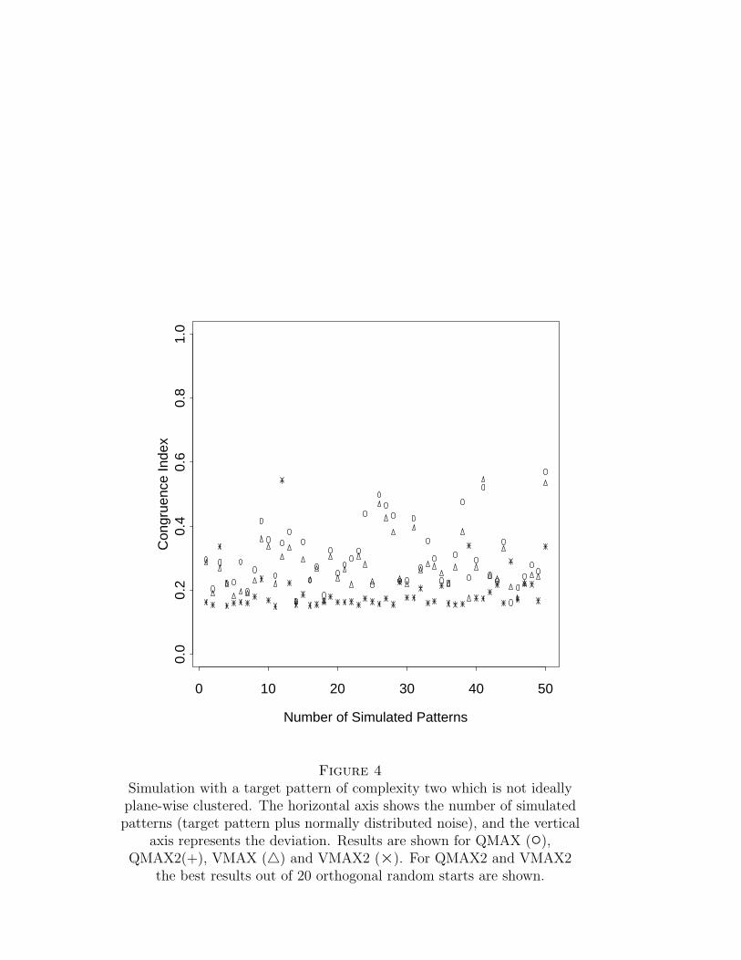
A third simulation experiment is also based on a matrix of loadings ofcomplexity two (i.e. two nonzero loadings on at most two factors), but therows of this target pattern are not ideally plane-wise clustered. In moredetail, the target pattern is of the same size as before (p = 100 variablesand k = 4 factors), the first 40 variables have two nonzero loadings at thefirst two factors, the next 8 variables have two nonzero loadings at factors1 and 3, the next 7 variables at factors 1 and 4, the next 6 variables atfactors 2 and 3, and the remaining 39 variables have two nonzero loadingsat the last two factors. The nonzero loadings are constructed in the sameway as in the first simulation experiment. The pattern is contaminatedin each of 50 simulations with randomly distributed noise (according toN(0, 1/10)), and the resulting loadings are scrambled by random orthogonalrotations. For QMAX2 and VMAX2 the best solutions out of 20 randomizedstarting positions are taken. (The results of QMAX and VMAX are varying

9

only marginally for different orthogonal random starts.) Figure 4 presentsthe resulting congruence index (vertical axis) for each simulated pattern(horizontal axis). Although the solutions of the classical methods and themethods for rotation to principal planes are much closer now, the resultsof QMAX2 and VMAX2 are clearly better. The congruence index is lowerthan 0.2 for about 75% of the results of QMAX2 and VMAX2, but justfor 15% of VMAX and not even for 10% of QMAX. Like in the previousexperiments, the results for QMAX2 and VMAX2 are very similar. Theaverage congruence indices are: 0.30 for QMAX, 0.28 for VMAX, and 0.19for both QMAX2 and VMAX2. When taking the best solutions out of 10instead of 20 orthogonal random starts, the average congruence increases to0.23 for QMAX2 and VMAX2.


The simulation was done on a Pentium PC with 120 MHz. Consideringthe first simulation experiment, the mean computation time over all 50 repli-cations for QMAX, QMAX2, VMAX and VMAX2 is reported in Table 1.The values for QMAX2 and VMAX2 correspond to the time needed for oneout of E different plane combinations (see (4)). Table 1 also summarizes themean computation time for the rotation of 6, 8, 10 and 12 factors. VMAX2needs about twice as much computation time as QMAX2, and there is abig difference between the time for classical rotation and rotation to planes(almost factor 100 for VMAX2). Since the values for QMAX2 and VMAX2have to be multiplied by the number E of different plane combinations, theproposed algorithm becomes impractical for a larger number of factors.

Table 1 is inserted about here.

The previous simulation experiments have shown how well QMAX2 andVMAX2 perform with matrices of loadings with complexity two. However,what would happen when rotating matrices of loadings with complexityone? As an example we consider the pattern shown in the left part of Table2 (p = 8 and k = 4). The middle part of Table 2 shows the result forboth QMAX and VMAX rotation. The true pattern is perfectly recoveredby these methods. Finally, the right part of Table 2 shows the generalresult for QMAX2 and VMAX2, where the first two factors span the firstprincipal plane and the last two factors the second principal plane. a, b, c

10

and d are real numbers within the interval -1 and 1 with the restrictionsa2 + b2 = c2 + d2 = 1. This means that an infinite number of solutionsfor QMAX2 and VMAX2 is possible, each obtained by orthogonal rotationof the principal planes. The reason for this phenomenon can be found byconsidering the rotation algorithm (section 3). The pairwise rotations areonly performed for pairs of factors of different planes; rotations within aprincipal plane are not necessary because the resulting plane will not giveany new information.


5. Example

In this section a data set is considered which origins from a cooperationbetween the research institutes Studia (Schlierbach, Austria) and Albtum(Weihenstephan, Germany). More than 800 variables from different fieldswere measured in the 96 Bavarian districts and cities, mainly in the year1987. Detailed information can be found in a technical report (Studia andAlbtum, 1993).

For reason of clarity nine variables are selected: rate of unemployment(1), median salary (2), percentage of the population in the age 6-15 years (3),percentage of the population older that 60 years (4), percentage of divorcedpersons (5), percentage of commuters (6), average number of persons perhousehold (7), percentage of larceny delicts (8), and percentage of stomachcancer as cause of death (9).

The choice of four factors gives a proportion of explained variation ofabout 93%. Principal common factor analysis without rotation of the factorsresults in the loadings presented in the left part of Table 3. The loadingsafter classical varimax rotation are shown in the right part of Table 3.


The unrotated matrix of loadings is basis for varimax rotation to prin-cipal planes. The best result (maximum of the objective function) of theloadings for 10 orthogonal random starts is shown in the left part of Table4. The first principal plane (PPL1) is spanned by the factors F1 and F2,

11

the second principal plane (PPL2) by F3 and F4. The right part of Table4 summarizes the contribution of each variable to the VMAX2 criterionand the sum over all single contributions for both, the resulting principalplanes from VMAX2 rotation and the planes spanned by F1-F3 and F2-F4resulting from VMAX rotation. The latter factor combinations give themaximum sum of the single contributions, and hence these planes allow thebest two-dimensional representation of the VMAX loadings.

The contribution of a variable to the VMAX2 criterion is high if thisvariable is well presented by only one plane. Variable 1 hence has highcontribution to PPL2 but low (negative) contribution to PPL1 where theloadings are close to zero. Variables 2 and 6 are not well presented bythe principal planes. All other variables (except variable 4) have highercontributions with VMAX2 rotation than with VMAX rotation. Also thesum over the single contributions is higher for VMAX2 which means thatVMAX2 rotation separates the variables into planes in a better way.


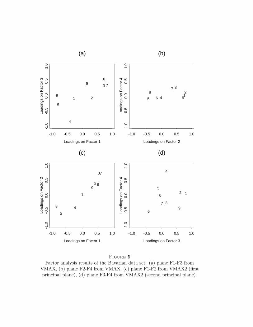
Figure 5 shows the resulting planes from VMAX and VMAX2 rotation.Figure 5a and 5b represent the planes spanned by F1-F3 and F2-F4 fromVMAX, respectively (see Table 3), and Figure 5c and 5d show PPL1 andPPL2 from VMAX2, respectively (see Table 4). The first planes fromVMAX and VMAX2 (Figure 5a and 5c) show some similarity, whereas thesecond planes (Figure 5b and 5d) reveal big differences. Variables 1, 2, 4,6 and 9 are well presented by PPL2 (large distance to the center), but notwell presented by PPL1 (close to the center). Similarly, variables 3, 5, 7 and8 are very well presented by PPL1, but at the same time they are close tothe center in PPL2. The variables in the second plane from VMAX rotationare mainly arranged along the direction of factor 2, whereas in PPL2 thevariables are spread over the whole plane. PPL2 hence makes the connec-tions between variables 1, 2, 4, 6 and 9 visible and allows interpretationsfor these relationships. In this example, however, one still has to be carefulwith interpretations, since connections can also be caused by other variableswhich have not been analyzed. Therefore it is advisable to take the wholedata set for a detailed investigation.


12

6. Summary

The idea of simple structure for planes is an extension of the classicalsimple structure. In the classical case the rotated factors should be asseparated as possible, i.e. each row of the rotated loadings matrix shouldcontain only a few high loadings, the remaining loadings should be low.Simple structure for planes is constructed in that way to obtain planes whichare as separated as possible: For each variable there should be only a fewhigh “loadings on planes”, which are expressed by the multiple correlation(2), otherwise low values are desired. The advantage of this extension isthat the resulting principal planes are aimed to be disjoint. Hence, by justpresenting the principal planes, most information of the matrix of loadingsis given. Since graphical presentations of the loadings by planes are easy tosurvey, especially in connection with factor scores like in a biplot (Gabriel,1971), this is a desired property. For classical rotation methods, usually allpairs of factors have to be shown for a detailed (2-dimensional) presentationof the loadings.

Another property which results from the construction of two-dimensionalsimple structure is that for each principal plane a maximum number ofvariables is not near the origin. Hence, these variables are well presentedby the plane and the interpretation of relationships between these variablesare more reliable.

Analytic solutions of the rotation methods QMAX2 and VMAX2 canbe found by the proposed algorithm. In each step the objective functionincreases monotonically. However, the algorithm often leads to local opti-mality, and the global optimum has to be approximated by applying thealgorithm with several orthogonal random starts. The simulation exampleshave shown that 10 to 20 orthogonal random starts are sufficient for re-covering complicated target patterns. However, for applications it is moreadvisable not to fix the number of randomizations but to continue on search-ing so long as additional tries have a good chance of improving the solutionsalready in store.

The proposed algorithm becomes impractical for a larger number offactors. Since the mean computation times given in Table 1 have to bemultiplied by the number of different plane combinations, VMAX2 rotationfor 10 factors would need about 100.000 seconds for one orthogonal randomstart at the computer used for this study. However, it turned out thatin most cases different plane combinations did not result in new solutions.Further investigation has to be done in examining how many combinationsare sufficient for finding the best result.

In section 2 it was suggested that for an odd number of factors one factor

13

should be omitted for principal plane rotation. Since the number of factorsto be retained in factor analysis is often a hard decision, it could be moreadvisable to retain always an even number of factors.

The simulation has shown that QMAX2 and VMAX2 often give the sameresult. In most applications one would prefer VMAX2 because it turned outthat QMAX2 leads to a main first plane, as the classical quartimax-criterionhas the tendency to converge over a main first vector (Kaiser, 1956, 1958).

If the complexity of a pattern is one (or close to one), the rotated pat-tern obtained by QMAX2 and VMAX2 can be transformed to the patternobtained by QMAX and VMAX by an orthogonal rotation (see Table 2).The solution from QMAX2 and VMAX2 can be seen as an alternative repre-sentation of the original pattern. Hence, in that case QMAX2 and VMAX2are not competitors of the classical rotation criteria.

It is possible to extend the ideas and formulas of simple structure forplanes to simple structure for higher dimensions. The results which we callprincipal spaces have the same properties as principal planes.

References

Baaske, W. (1988). Principal planes: visual structure analysis by clusterbiplot projection pursuit in a multinational survey. Applied Mathe-matics and Computation, 26, 303-314.

Carroll, J.B. (1953). An analytic solution for approximating simple struc-ture in factor analysis. Psychometrika, 18, 23-38.

Friedman, J.H. (1987). Exploratory projection pursuit. Journal of theAmerican Statistical Association, 82(397), 249-266.

Gabriel, K.R. (1971). The biplot graphic display of matrices with applica-tion to principal component analysis. Biometrika, 58(3), 453-467.

Gebhardt, F. (1968). A counterexample to two-dimensional varimax-rotation. Psychometrika, 33, 35-36.

Golub, G.H., and Ortega, J.M. (1993). Scientific computing, An introduc-tion with parallel computing. New York: Academic Press.

Huber, P.J. (1985). Projection Pursuit. The Annals of Statistics, 13/2,435-475.

Kaiser, H.F. (1956). Note on Carroll’s analytic simple structure. Psy-chometrika, 21, 89-92.

14

Kaiser, H.F. (1958). The varimax criterion for analytic rotation in factoranalysis. Psychometrika, 23, 187-200.

Mardia, K.V., Kent J.T., and Bibby, J.M. (1979). Multivariate Analysis.London: Academic Press.

Studia and Albtum (1993). Externe Leistungen der bauerlichen Land-wirtschaft in Bayern. Technical report. STUDIA - Research Group forInternational Analyses, Schlierbach; ALBTUM - Professorship for Ap-plied Agricultural Business Economics, Freising-Weihenstephan, Mu-nich University of Technology. In German.

ten Berge, J.M.F. (1984). A joint treatment of varimax rotation and theproblem of diagonalizing symmetric matrices simultaneously in theleast-squares sense. Psychometrika, 48, 347-358.

Thurstone, L.L. (1944). Second-order factors. Psychometrika, 9, 71-100.

15

Figure 1Regula-falsi algorithm for maximizing the VMAX2 criterion in one plane.f is the function defined by the criterion, and f ′ is the derivative of f .

Figure 2Simulation experiment with an ideally plane-wise clustered target patternof complexity two. The horizontal axis shows the number of replications

(orthogonal random starts), and the vertical axis represents the congruenceindex (16) as a measure of deviation from the original pattern. Results are

shown for QMAX (◦), QMAX2(+), VMAX (4) and VMAX2 (×).

Figure 3Simulation with the same target pattern as in Figure 2 with additional

random noise. The horizontal axis shows the number of simulatedpatterns, and the vertical axis represents the congruence index. Resultsare shown for QMAX (◦), QMAX2(+), VMAX (4) and VMAX2 (×).For QMAX2 and VMAX2 the best results out of 10 orthogonal random

starts are shown.

Figure 4Simulation with a target pattern of complexity two which is not ideallyplane-wise clustered. The horizontal axis shows the number of simulatedpatterns (target pattern plus normally distributed noise), and the vertical

axis represents the deviation. Results are shown for QMAX (◦),QMAX2(+), VMAX (4) and VMAX2 (×). For QMAX2 and VMAX2

the best results out of 20 orthogonal random starts are shown.

Figure 5Factor analysis results of the Bavarian data set: (a) plane F1-F3 from

VMAX, (b) plane F2-F4 from VMAX, (c) plane F1-F2 from VMAX2 (firstprincipal plane), (d) plane F3-F4 from VMAX2 (second principal plane).

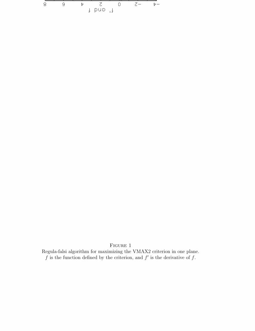
Figure 1Regula-falsi algorithm for maximizing the VMAX2 criterion in one plane.f is the function defined by the criterion, and f ′ is the derivative of f .

Number of Simulated Patterns

Con

grue

nce

Inde

x

0 10 20 30 40 50

0.0

0.2

0.4

0.6

0.8

1.0

Figure 2Simulation experiment with an ideally plane-wise clustered target patternof complexity two. The horizontal axis shows the number of replications

(orthogonal random starts), and the vertical axis represents the congruenceindex (16) as a measure of deviation from the original pattern. Results are

shown for QMAX (◦), QMAX2(+), VMAX (4) and VMAX2 (×).


Con

grue

nce

Inde

x

0 10 20 30 40 50

0.0

0.2

0.4

0.6

0.8

1.0

Figure 3Simulation with the same target pattern as in Figure 2 with additional

random noise. The horizontal axis shows the number of simulatedpatterns, and the vertical axis represents the congruence index. Resultsare shown for QMAX (◦), QMAX2(+), VMAX (4) and VMAX2 (×).For QMAX2 and VMAX2 the best results out of 10 orthogonal random

starts are shown.


Con

grue

nce

Inde

x

0 10 20 30 40 50

0.0

0.2

0.4

0.6

0.8

1.0

Figure 4Simulation with a target pattern of complexity two which is not ideallyplane-wise clustered. The horizontal axis shows the number of simulatedpatterns (target pattern plus normally distributed noise), and the vertical

axis represents the deviation. Results are shown for QMAX (◦),QMAX2(+), VMAX (4) and VMAX2 (×). For QMAX2 and VMAX2

the best results out of 20 orthogonal random starts are shown.

Loadings on Factor 1

Load

ings

on

Fac

tor

3

-1.0 -0.5 0.0 0.5 1.0

-1.0

-0.5

0.0

0.5

1.0

1 2

3

4

5

6

7

8

9

(a)


Load

ings

on

Fac

tor

4

-1.0 -0.5 0.0 0.5 1.0

-1.0

-0.5

0.0

0.5

1.0

12

3

45 6

78

9

(b)


Load

ings

on

Fac

tor

2

-1.0 -0.5 0.0 0.5 1.0

-1.0

-0.5

0.0

0.5

1.0

1

2

3

45

6

7

8

9

(c)


Load

ings

on

Fac

tor

4

-1.0 -0.5 0.0 0.5 1.0

-1.0

-0.5

0.0

0.5

1.0

12

3

4

5

6

7

8

9

(d)

Figure 5Factor analysis results of the Bavarian data set: (a) plane F1-F3 from

VMAX, (b) plane F2-F4 from VMAX, (c) plane F1-F2 from VMAX2 (firstprincipal plane), (d) plane F3-F4 from VMAX2 (second principal plane).

Table 1Mean computation time for one out of E combinations of planes (in

seconds), for 2 planes (4 factors) to 6 planes (12 factors) at the basis of 50replications of a simulation.

Rotation Number of FactorsMethod 4 6 8 10 12QMAX 0.16 0.44 0.94 2.72 6.81QMAX2 2.39 19.23 34.88 46.67 96.70VMAX 0.11 0.33 0.82 1.65 2.47VMAX2 4.70 34.44 76.84 105.66 199.49

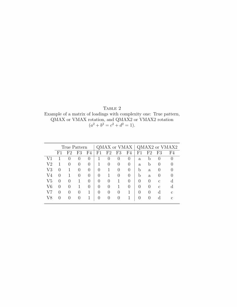
Table 2Example of a matrix of loadings with complexity one: True pattern,

QMAX or VMAX rotation, and QMAX2 or VMAX2 rotation(a2 + b2 = c2 + d2 = 1).

True Pattern QMAX or VMAX QMAX2 or VMAX2F1 F2 F3 F4 F1 F2 F3 F4 F1 F2 F3 F4

V1 1 0 0 0 1 0 0 0 a b 0 0V2 1 0 0 0 1 0 0 0 a b 0 0V3 0 1 0 0 0 1 0 0 b a 0 0V4 0 1 0 0 0 1 0 0 b a 0 0V5 0 0 1 0 0 0 1 0 0 0 c dV6 0 0 1 0 0 0 1 0 0 0 c dV7 0 0 0 1 0 0 0 1 0 0 d cV8 0 0 0 1 0 0 0 1 0 0 d c

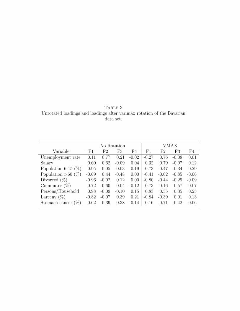
Table 3Unrotated loadings and loadings after varimax rotation of the Bavarian

data set.

No Rotation VMAXVariable F1 F2 F3 F4 F1 F2 F3 F4

Unemployment rate 0.11 0.77 0.21 -0.02 -0.27 0.76 -0.08 0.01Salary 0.60 0.62 -0.09 0.04 0.32 0.79 -0.07 0.12Population 6-15 (%) 0.95 0.05 -0.03 0.19 0.73 0.47 0.34 0.29Population >60 (%) -0.69 0.44 -0.48 0.00 -0.41 -0.02 -0.85 -0.06Divorced (%) -0.96 -0.02 0.12 0.00 -0.80 -0.44 -0.29 -0.09Commuter (%) 0.72 -0.60 0.04 -0.12 0.73 -0.16 0.57 -0.07Persons/Household 0.98 -0.09 -0.10 0.15 0.83 0.35 0.35 0.25Larceny (%) -0.82 -0.07 0.39 0.21 -0.84 -0.39 0.01 0.13Stomach cancer (%) 0.62 0.39 0.38 -0.14 0.16 0.71 0.42 -0.06

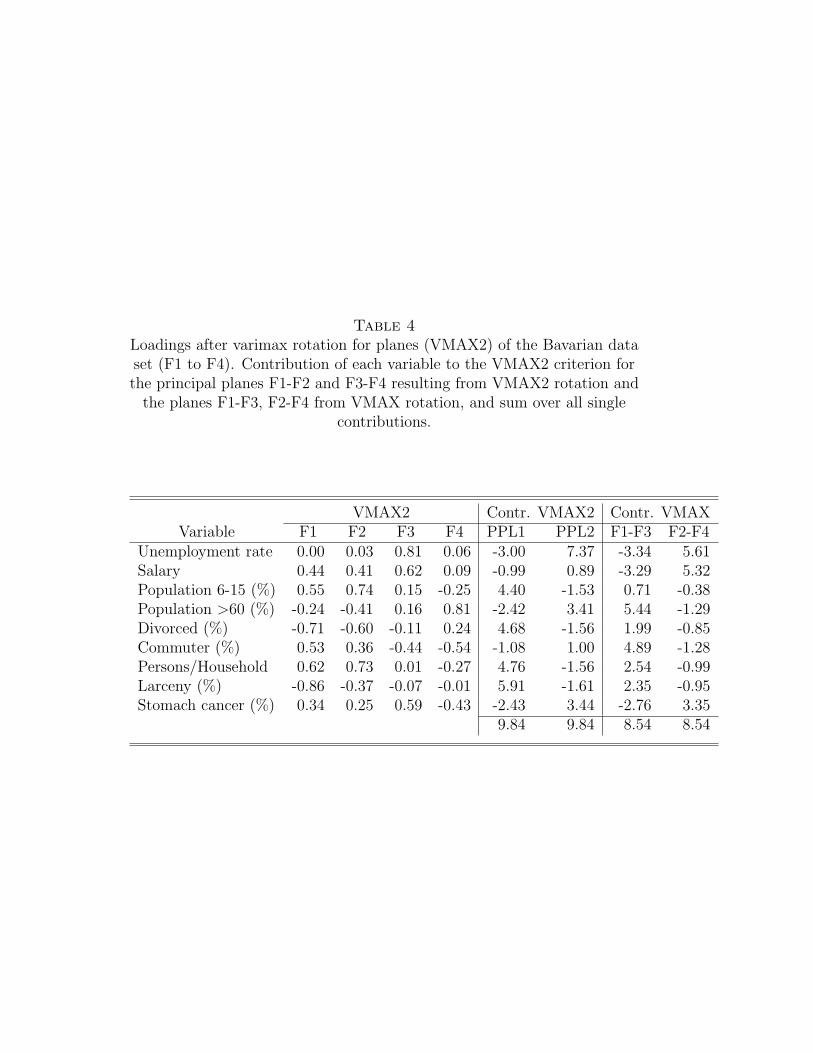
Table 4Loadings after varimax rotation for planes (VMAX2) of the Bavarian dataset (F1 to F4). Contribution of each variable to the VMAX2 criterion forthe principal planes F1-F2 and F3-F4 resulting from VMAX2 rotation and

the planes F1-F3, F2-F4 from VMAX rotation, and sum over all singlecontributions.

VMAX2 Contr. VMAX2 Contr. VMAXVariable F1 F2 F3 F4 PPL1 PPL2 F1-F3 F2-F4

Unemployment rate 0.00 0.03 0.81 0.06 -3.00 7.37 -3.34 5.61Salary 0.44 0.41 0.62 0.09 -0.99 0.89 -3.29 5.32Population 6-15 (%) 0.55 0.74 0.15 -0.25 4.40 -1.53 0.71 -0.38Population >60 (%) -0.24 -0.41 0.16 0.81 -2.42 3.41 5.44 -1.29Divorced (%) -0.71 -0.60 -0.11 0.24 4.68 -1.56 1.99 -0.85Commuter (%) 0.53 0.36 -0.44 -0.54 -1.08 1.00 4.89 -1.28Persons/Household 0.62 0.73 0.01 -0.27 4.76 -1.56 2.54 -0.99Larceny (%) -0.86 -0.37 -0.07 -0.01 5.91 -1.61 2.35 -0.95Stomach cancer (%) 0.34 0.25 0.59 -0.43 -2.43 3.44 -2.76 3.35

9.84 9.84 8.54 8.54

Table 1Mean computation time for one out of E combinations of planes (in

seconds), for 2 planes (4 factors) to 6 planes (12 factors) at the basis of 50replications of a simulation.

Table 2Example of a matrix of loadings with complexity one: True pattern,

QMAX or VMAX rotation, and QMAX2 or VMAX2 rotation(a2 + b2 = c2 + d2 = 1).

Table 3Unrotated loadings and loadings after varimax rotation of the Bavarian

data.

Table 4Loadings after varimax rotation for planes (VMAX2) of the Bavarian dataset (F1 to F4). Contribution of each variable to the VMAX2 criterion forthe principal planes F1-F2 and F3-F4 resulting from VMAX2 rotation and

the planes F1-F3, F2-F4 from VMAX rotation, and sum over all singlecontributions.

ORTHOGONAL PRINCIPAL PLANES

Peter Filzmoser1

department of statistics, probability theory and actuarialmathematics

vienna university of technology, austria

1Department of Statistics, Probability Theory and Actuarial Mathematics, ViennaUniversity of Technology, Wiedner Hauptstr. 8-10, A–1040 Vienna, Austria.The author is most grateful to the referees, the Associate Editor, and the Editor for help-ful suggestions, which resulted in a completely improved version of an earlier manuscript.

Abstract

Factor analysis and principal component analysis result in com-puting a new co-ordinate system, which is usually rotated to ob-tain a better interpretation of the results. In the present paper, theidea of rotation to simple structure is extended to two dimensions.While the classical definition of simple structure is aimed at rotat-ing (one-dimensional) factors, the extension to a simple structure fortwo dimensions is based on the rotation of planes. The resultingplanes (principal planes) reveal a better view of the data than planesspanned by factors from classical rotation and hence allow a morereliable interpretation. The usefulness of the method as well as theeffectiveness of a proposed algorithm are demonstrated by simulationexperiments and an example.

Key words: principal component analysis, factor analysis, orthogonalrotation, simple structure.

Documents

ORTHOGONAL PRINCIPAL PLANES