Embed Size (px)
Citation preview

Orthogonal Laplacianfaces for Face Recognition
Deng Cai ∗
Department of Computer Science
University of Illinois at Urbana Champaign
1334 Siebel Center, 201 N. Goodwin Ave, Urbana, IL 61801, USA
Phone: (217) 344-2189
Xiaofei He
Yahoo Research Labs
3333 W Empire Avenue, Burbank, CA 91504, USA
Phone: (818) 524-3545
Jiawei Han, ACM Fellow
Department of Computer Science
University of Illinois at Urbana Champaign
2132 Siebel Center, 201 N. Goodwin Ave, Urbana, IL 61801, USA
Phone: (217) 333-6903
Fax: (217) 265-6494
Hong-Jiang Zhang, IEEE Fellow
Microsoft Research Asia
3F Beijing Sigma Center, No. 49, Zhichun Road, Beijing 100080, P. R. China
∗corresponding author
1
Abstract
Following the intuition that the naturally occurring face data may be generated by sampling
a probability distribution that has support on or near a sub-manifold of ambient space, we
propose an appearance-based face recognition method, called Orthogonal Laplacianface (OLPP).
Our algorithm is based on the Locality Preserving Projection (LPP) algorithm, which aims at
finding a linear approximation to the eigenfunctions of the Laplace Beltrami operator on the face
manifold. However, LPP is non-orthogonal and this makes it difficult to reconstruct the data.
The OLPP method produces orthogonal basis functions and can have more locality preserving
power than LPP. Since the locality preserving power is potentially related to the discriminating
power, the OLPP is expected to have more discriminating power than LPP. Experimental results
on three face databases demonstrate the effectiveness of our proposed algorithm.
Keywords
Appearance-based vision, face recognition, Locality preserving projection, Orthogonal locality pre-
serving projection,
1 INTRODUCTION
Recently, appearance-based face recognition has received a lot of attention [20][14]. In general, a
face image of size n1 × n2 is represented as a vector in the image space Rn1×n2 . We denote by face
space the set of all the face images. Though the image space is very high dimensional, the face
space is usually a submanifold of very low dimensionality which is embedded in the ambient space.
A common way to attempt to resolve this problem is to use dimensionality reduction techniques
[1][2][8][12][11][17]. The most popular methods discovering the face manifold structure include
Eigenface [20], Fisherface [2], and Laplacianface [9].
Face representation is fundamentally related to the problem of manifold learning [3][16][19]
which is an emerging research area. Given a set of high-dimensional data points, manifold learning
techniques aim at discovering the geometric properties of the data space, such as its Euclidean
embedding, intrinsic dimensionality, connected components, homology, etc. Particularly, learning
representation is closely related to the embedding problem, while clustering can be thought of as
1
finding connected components. Finding a Euclidean embedding of the face space for recognition
is the primary focus of our work in this paper. Manifold learning techniques can be classified
into linear and non-linear techniques. For face processing, we are especially interested in linear
techniques due to the consideration of computational complexity.
The Eigenface and Fisherface methods are two of the most popular linear techniques for face
recognition. Eigenface applies Principal Component Analysis [6] to project the data points along
the directions of maximal variances. The Eigenface method is guaranteed to discover the intrinsic
geometry of the face manifold when it is linear. Unlike the Eigenface method which is unsupervised,
the Fisherface method is supervised. Fisherface applies Linear Discriminant Analysis to project the
data points along the directions optimal for discrimination. Both Eigenface and Fisherface see only
the global Euclidean structure. The Laplacianface method [9] is recently proposed to model the
local manifold structure. The Laplacianfaces are the linear approximations to the eigenfunctions
of the Laplace Beltrami operator on the face manifold. However, the basis functions obtained by
the Laplacianface method are non-orthogonal. This makes it difficult to reconstruct the data.
In this paper, we propose a new algorithm called Orthogonal Laplacianface. O-Laplacianface
is fundamentally based on the Laplacianface method. It builds an adjacency graph which can best
reflect the geometry of the face manifold and the class relationship between the sample points. The
projections are then obtained by preserving such a graph structure. It shares the same locality
preserving character as Laplacianface, but at the same time it requires the basis functions to be
orthogonal. Orthogonal basis functions preserve the metric structure of the face space. In fact,
if we use all the dimensions obtained by O-Laplacianface, the projective map is simply a rotation
map which does not distort the metric structure. Moreover, our empirical study shows that O-
Laplacianface can have more locality preserving power than Laplacianface. Since it has been
shown that the locality preserving power is directly related to the discriminating power [9], the
O-Laplacianface is expected to have more discriminating power than Laplacianface.
The rest of the paper is organized as follows. In Section 2, we give a brief review of the Lapla-
cianface algorithm. Section 3 introduces our O-Laplacianface algorithm. We provide a theoretical
justification of our algorithm in Section 4. Extensive experimental results on face recognition are
presented in Section 5. Finally, we provide some concluding remarks and suggestions for future
work in Section 6.
2
2 A BRIEF REVIEW OF LAPLACIANFACE
Laplacianface is a recently proposed linear method for face representation and recognition. It is
based on Locality Preserving Projection [10] and explicitly considers the manifold structure of the
face space.
Given a set of face images {x1, · · · ,xn} ⊂ Rm, let X = [x1,x2, · · · ,xn]. Let S be a similar-
ity matrix defined on the data points. Laplacianface can be obtained by solving the following
minimization problem:
aopt = arg mina
m∑
i=1
m∑
j=1
(
aTxi − aTxj
)2Sij
= arg mina
aT XLXTa
with the constraint
aT XDXTa = 1
where L = D − S is the graph Laplacian [4] and Dii =∑
j Sij . Dii measures the local density
around xi. Laplacianface constructs the similarity matrix S as:
Sij =
e−‖xi−xj‖
2
t , if xi is among the p nearest
neighbors of xj or xj is among
the p nearest neighbors of xi
0, otherwise.
Here Sij is actually heat kernel weight, the justification for such choice and the setting of the
parameter t can be referred to [3].
The objective function in Laplacianface incurs a heavy penalty if neighboring points xi and xj
are mapped far apart. Therefore, minimizing it is an attempt to ensure that if xi and xj are “close”
then yi (= aTxi) and yj (= aTxj) are close as well [9]. Finally, the basis functions of Laplacianface
are the eigenvectors associated with the smallest eigenvalues of the following generalized eigen-
problem:
XLXTa = λXDXTa
XDXT is non-singular after some pre-processing steps on X in Laplacianface, thus, the basis
functions of Laplacianface can also be regarded as the eigenvectors of the matrix (XDXT )−1XLXT
3
associated with the smallest eigenvalues. Since (XDXT )−1XLXT is not symmetric in general, the
basis functions of Laplacianface are non-orthogonal.
Once the eigenvectors are computed, let Ak = [a1, · · · ,ak] be the transformation matrix. Thus,
the Euclidean distance between two data points in the reduced space can be computed as follows:
dist(yi,yj) = ‖yi − yj‖
= ‖ATxi − ATxj‖
= ‖AT (xi − xj)‖
=√
(xi − xj)T AAT (xi − xj)
If A is an orthogonal matrix, AAT = I and the metric structure is preserved.
3 THE ALGORITHM
In this Section, we introduce a novel subspace learning algorithm, called Orthogonal Locality
Preserving Projection (OLPP). Our Orthogonal Laplacianface algorithm for face representation
and recognition is based on OLPP. The theoretical justifications of our algorithm will be presented
in Section 4.
In appearance-based face analysis one is often confronted with the fact that the dimension of
the face image vector (m) is much larger than the number of face images (n). Thus, the m × m
matrix XDXT is singular. To overcome this problem, we can first apply PCA to project the faces
into a subspace without losing any information and the matrix XDXT becomes non-singular.
The algorithmic procedure of OLPP is stated below.
1. PCA Projection: We project the face images xi into the PCA subspace by throwing away
the components corresponding to zero eigenvalue. We denote the transformation matrix of
PCA by WPCA. By PCA projection, the extracted features are statistically uncorrelated and
the rank of the new data matrix is equal to the number of features (dimensions).
2. Constructing the Adjacency Graph: Let G denote a graph with n nodes. The i-th node
corresponds to the face image xi. We put an edge between nodes i and j if xi and xj are
“close”, i.e. xi is among p nearest neighbors of xj or xj is among p nearest neighbors of
4
xi. Note that, if the class information is available, we simply put an edge between two data
points belonging to the same class.
3. Choosing the Weights: If node i and j are connected, put
Sij = e−‖xi−xj‖
2
t
Otherwise, put Sij = 0. The weight matrix S of graph G models the local structure of the
face manifold. The justification of this weight can be traced back to [3].
4. Computing the Orthogonal Basis Functions: We define D as a diagonal matrix whose
entries are column (or row, since S is symmetric) sums of S, Dii =∑
j Sji. We also define
L = D−S, which is called Laplacian matrix in spectral graph theory [4]. Let {a1,a2, · · · ,ak}
be the orthogonal basis vectors, we define:
A(k−1) = [a1, · · · ,ak−1]
B(k−1) =[
A(k−1)]T
(XDXT )−1A(k−1)
The orthogonal basis vectors {a1,a2, · · · ,ak} can be computed as follow.
• Compute a1 as the eigenvector of (XDXT )−1XLXT associated with the smallest eigen-
value.
• Compute ak as the eigenvector of
M (k) =
{
I − (XDXT )−1A(k−1)[
B(k−1)]−1 [
A(k−1)]T
}
· (XDXT )−1XLXT
associated with the smallest eigenvalue of M (k).
5. OLPP Embedding: Let WOLPP = [a1, · · · ,al], the embedding is as follows.
x → y = W Tx
W = WPCAWOLPP
where y is a l-dimensional representation of the face image x, and W is the transformation
matrix.
5
4 JUSTIFICATIONS
In this section, we provide theoretical justifications of our proposed algorithm.
4.1 Optimal Orthogonal Embedding
We begin with the following definition.
Definition Let a ∈ Rm be a projective map. The Locality Preserving Function f is defined
as follows.
f(a) =aT XLXTa
aT XDXTa(1)
Consider the data are sampled from an underlying data manifold M. Suppose we have a map
g : M → R. The gradient ∇g(x) is a vector field on the manifold, such that for small δx
|g(x + δx) − g(x)| ≈ |〈∇g(x), δx〉| ≤ ‖∇g‖‖δx‖
Thus we see that if ‖∇g‖ is small, points near x will be mapped to points near g(x). We can use
∫
M‖∇g(x)‖2dx
∫
M|g(x)|2dx
(2)
to measure the locality preserving power on average of the map g [3]. With finite number of samples
X and a linear projective map a, f(a) is a discrete approximation of equation (2) [10]. Similarly,
f(a) evaluates the locality preserving power of the projective map a.
Directly minimizing the function f(a) will lead to the original Laplacianface (LPP) algorithm.
Our O-Laplacianface (OLPP) algorithm tries to find a set of orthogonal basis vectors a1, · · · ,ak
which minimizes the locality preserving function. Thus, a1, · · · ,ak are the set of vectors minimizing
f(a) subject to the constraint aTk a1 = aT
k a2 = · · · = aTk ak−1 = 0.
The objective function of OLPP can be written as,
a1 = arg mina
aT XLXTa
aT XDXTa(3)
and,
ak = arg mina
aT XLXTa
aT XDXTa(4)
subject to aTk a1 = aT
k a2 = · · · = aTk ak−1 = 0
6
Since XDXT is positive definite after PCA projection, for any a, we can always normalize it such
that aT XDXTa = 1, and the ratio of aT XLXTa and aT XDXTa remains unchanged. Thus, the
above minimization problem is equivalent to minimizing the value of aT XLXTa with an additional
constraint as follows,
aT XDXTa = 1
Note that, the above normalization is only for simplifying the computation. Once we get the
optimal solutions, we can re-normalize them to get an orthonormal basis vectors.
It is easy to check that a1 is the eigenvector of the generalized eigen-problem:
XLXTa = λXDXTa
associated with the smallest eigenvalue. Since XDXT is non-singular, a1 is the eigenvector of the
matrix (XDXT )−1XLXT associated with the smallest eigenvalue.
In order to get the k-th basis vector, we minimize the following objective function:
f(ak) =aT
k XLXTak
aTk XDXTak
(5)
with the constraints:
aTk a1 = aT
k a2 = · · · = aTk ak−1 = 0, aT
k XDXTak = 1
We can use the Lagrange multipliers to transform the above objective function to include all
the constraints
C(k) = aTk XLXTak − λ
(
aTk XDXTak − 1
)
− µ1aTk a1 − · · · − µk−1a
Tk ak−1
The optimization is performed by setting the partial derivative of C(k) with respect to ak to zero:
∂C(k)
∂ak
= 0
⇒ 2XLXTak − 2λXDXTak − µ1a1 · · · − µk−1ak−1 = 0
(6)
Multiplying the left side of (6) by aTk , we obtain
2aTk XLXTak − 2λaT
k XDXTak = 0
⇒ λ =aT
k XLXTak
aTk XDXTak
(7)
7
Comparing to (5), λ exactly represents the expression to be minimized.
Multiplying the left side of (6) successively by aT1 (XDXT )−1, · · · , aT
k−1(XDXT )−1, we now
obtain a set of k − 1 equations:
µ1aT1 (XDXT )−1a1 + · · · + µk−1a
T1 (XDXT )−1ak−1 = 2aT
1 (XDXT )−1XLXTak
µ1aT2 (XDXT )−1a1 + · · · + µk−1a
T2 (XDXT )−1ak−1 = 2aT
2 (XDXT )−1XLXTak
· · · · · ·
µ1aTk−1(XDXT )−1a1 + · · · + µk−1a
Tk−1(XDXT )−1ak−1 = 2aT
k−1(XDXT )−1XLXTak
We define:
µ(k−1) = [µ1, · · · , µk−1]T , A(k−1) = [a1, · · · ,ak−1]
B(k−1) =[
B(k−1)ij
]
=[
A(k−1)]T
(XDXT )−1A(k−1)
B(k−1)ij = aT
i (XDXT )−1aj
Using this simplified notation, the previous set of k − 1 equations can be represented in a single
matrix relationship
B(k−1)µ(k−1) = 2[
A(k−1)]T
(XDXT )−1XLXTak
thus
µ(k−1) = 2[
B(k−1)]−1 [
A(k−1)]T
(XDXT )−1XLXTak (8)
Let us now multiply the left side of (6) by (XDXT )−1
2(XDXT )−1XLXTak − 2λak − µ1(XDXT )−1a1 − · · · − µk−1(XDXT )−1ak−1 = 0
This can be expressed using matrix notation as
2(XDXT )−1XLXTak − 2λak − (XDXT )−1A(k−1)µ(k−1) = 0
With equation (8), we obtain
{
I − (XDXT )−1A(k−1)[
B(k−1)]−1 [
A(k−1)]T
}
(XDXT )−1XLXTak = λak
As shown in (7), λ is just the criterion to be minimized, thus ak is the eigenvector of
M (k) =
{
I − (XDXT )−1A(k−1)[
B(k−1)]−1 [
A(k−1)]T
}
(XDXT )−1XLXT
8
0 200 400 600 800 1000 12000
0.2
0.4
0.6
0.8
1
Eigenvalues (OLPP vs. LPP)
OLPP
LPP
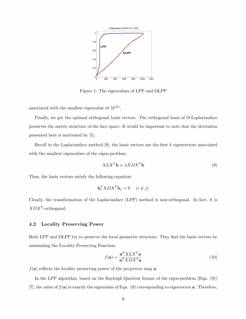
Figure 1: The eigenvalues of LPP and OLPP
associated with the smallest eigenvalue of M (k).
Finally, we get the optimal orthogonal basis vectors. The orthogonal basis of O-Laplacianface
preserves the metric structure of the face space. It would be important to note that the derivation
presented here is motivated by [5].
Recall in the Laplacianface method [9], the basis vectors are the first k eigenvectors associated
with the smallest eigenvalues of the eigen-problem:
XLXTb = λXDXTb (9)
Thus, the basis vectors satisfy the following equation:
bTi XDXTbj = 0 (i 6= j)
Clearly, the transformation of the Laplacianface (LPP) method is non-orthogonal. In fact, it is
XDXT -orthogonal.
4.2 Locality Preserving Power
Both LPP and OLPP try to preserve the local geometric structure. They find the basis vectors by
minimizing the Locality Preserving Function:
f(a) =aT XLXTa
aT XDXTa(10)
f(a) reflects the locality preserving power of the projective map a.
In the LPP algorithm, based on the Rayleigh Quotient format of the eigen-problem (Eqn. (9))
[7], the value of f(a) is exactly the eigenvalue of Eqn. (9) corresponding to eigenvector a. Therefore,
9
the eigenvalues of LPP reflect the locality preserving power of LPP. In OLPP, as we show in Eqn.
(7), the eigenvalues of OLPP also reflect its locality preserving power. This observation motivates
us to compare the eigenvalues of LPP and OLPP.
Fig. 1 shows the eigenvalues of LPP and OLPP. The data set used for this study is the PIE
face database (please see Section 5.2 for details). As can be seen, the eigenvalues of OLPP are con-
sistently smaller than those of LPP, which indicates that OLPP can have more locality preserving
power than LPP.
Since it has been shown in [9] that the locality preserving power is directly related to the
discriminating power, we expect that the O-Laplacianface (OLPP) based face representation and
recognition can obtain better performance than those based on Laplacianface (LPP).
5 EXPERIMENTAL RESULTS
In this section, we investigate the performance of our proposed O-Laplacianface method (PCA+OLPP)
for face representation and recognition. The system performance is compared with the Eigen-
face method (PCA) [21], the Fisherface method (PCA+LDA) [2] and the Laplacianface method
(PCA+LPP) [9], three of the most popular linear methods in face recognition. We use the same
graph structures in the Laplacianface and O-Laplacianface methods, which is built based on the
label information.
In this study, three face databases were tested. The first one is the Yale database1, the second
is the ORL (Olivetti Research Laboratory) database2, and the third is the PIE (pose, illumination,
and expression) database from CMU [18]. In all the experiments, preprocessing to locate the faces
was applied. Original images were manually aligned (two eyes were aligned at the same position),
cropped, and then re-sized to 32×32 pixels, with 256 gray levels per pixel. Each image is represented
by a 1, 024-dimensional vector in image space. Different pattern classifiers have been applied for
face recognition, such as nearest-neighbor [2], Bayesian [13], Support Vector Machine [15]. In this
paper, we apply the nearest-neighbor classifier for its simplicity. The Euclidean metric is used as
our distance measure.
1http://cvc.yale.edu/projects/yalefaces/yalefaces.html2http://www.uk.research.att.com/facedatabase.html
10
(a) Eigenfaces (b) Fisherfaces
(c) Laplacianfaces (d) O-Laplacianfaces
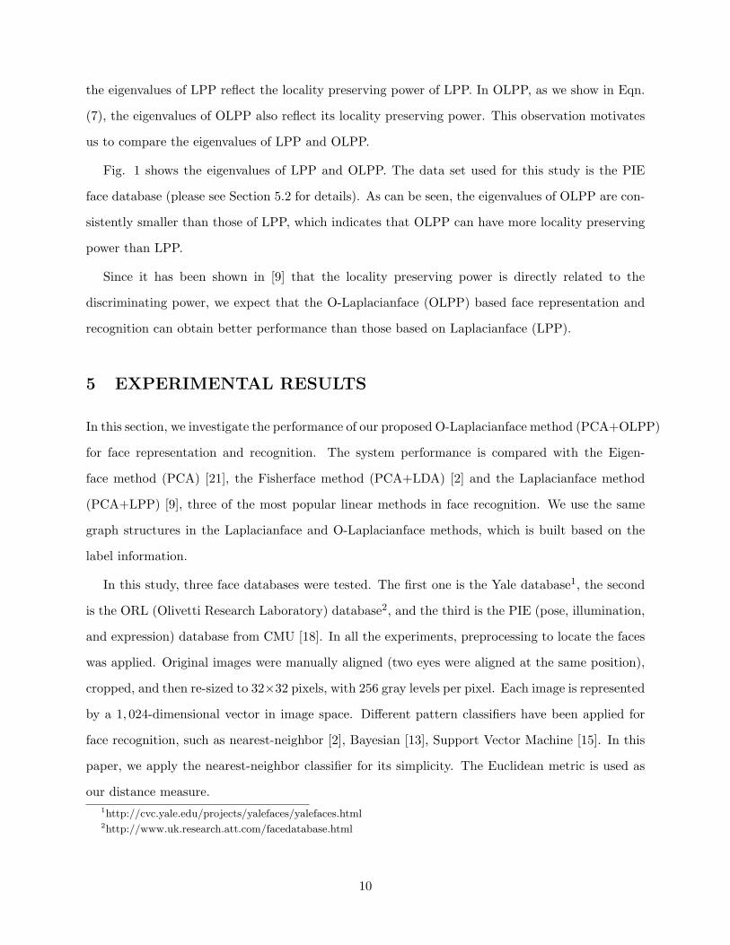
Figure 2: The first 6 Eigenfaces, Fisherfaces, Laplacianfaces, and O-Laplacianfaces calculated from
the face images in the ORL database.
Figure 3: Sample face images from the Yale database. For each subject, there are 11 face images
under different lighting conditions with facial expression.
In short, the recognition process has three steps. First, we calculate the face subspace from the
training samples; then the new face image to be identified is projected into d-dimensional subspace
by using our algorithm; finally, the new face image is identified by a nearest neighbor classifier.
We implemented all the algorithms in Matlab 7.04. The codes as well as the databases in Matlab
format can be downloaded at http://www.ews.uiuc.edu/~dengcai2/Data/data.html.
5.1 Face Representation using O-Laplacianfaces
In this sub-section, we compare the four algorithms for face representation, i.e., Eigenface, Fisher-
face, Laplacianface, and O-Laplacianface. For each of them, the basis vectors can be thought of as
the basis images and any other image is a linear combination of these basis images. It would be
interesting to see how these basis vectors look like in the image domain.
Using the ORL face database, we present the first 6 O-Laplacianfaces in Figure 2, together with
Eigenfaces, Fisherfaces, and Laplacianfaces.
11
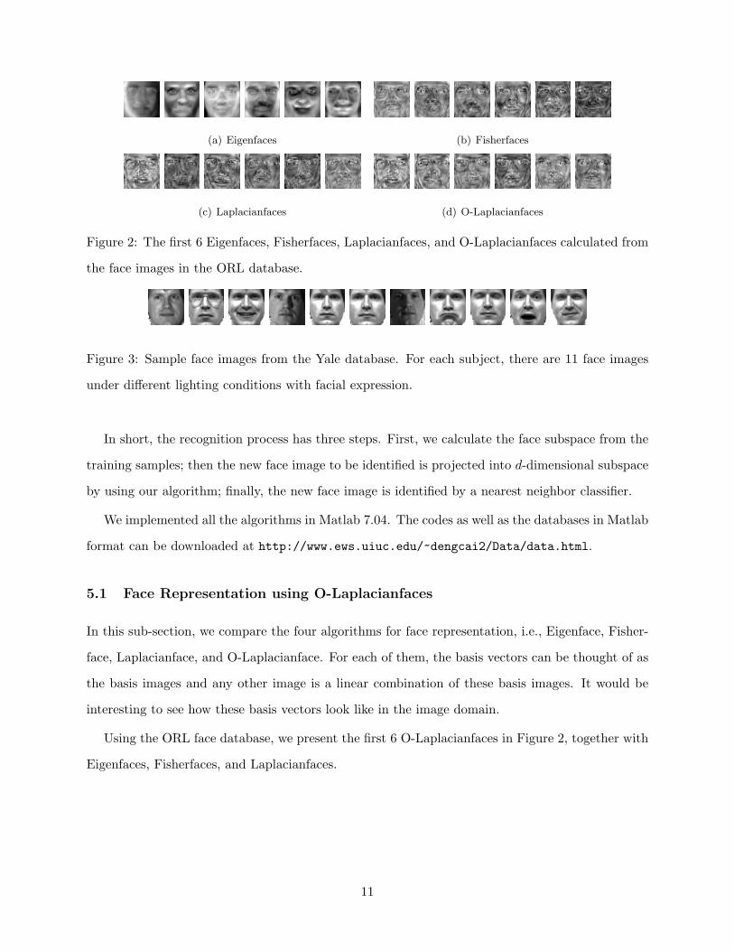
Table 1: Performance comparisons on the Yale database
Method 2 Train 3 Train 4 Train 5 Train
Baseline 56.5% 51.1% 47.8% 45.6%
Eigenfaces 56.5%(29) 51.1%(44) 47.8%(58) 45.2%(71)
Fisherfaces 54.3%(9) 35.5%(13) 27.3%(14) 22.5%(14)
Laplacianfaces 43.5%(14) 31.5%(14) 25.4%(14) 21.7%(14)
O-Laplacianfaces 44.3%(14) 29.9%(14) 22.7%(15) 17.9%(14)
0 5 10 15 20 25
45
50
55
60
65
70
75
80
Dims
Err
or
rate
(%
)
O-Laplacianfaces
Laplacianfaces
Fisherfaces
Eigenfaces
Baseline
(a) 2 Train
0 10 20 30 40
30
40
50
60
70
80
Dims
Err
or
rate
(%
)
O-Laplacianfaces
Laplacianfaces
Fisherfaces
Eigenfaces
Baseline
(b) 3 Train
0 20 40 6020
30
40
50
60
70
80
Dims
Err
or
rate
(%
)
O-Laplacianfaces
Laplacianfaces
Fisherfaces
Eigenfaces
Baseline
(c) 4 Train
0 20 40 60
20
30
40
50
60
70
80
Dims
Err
or
rate
(%
)
O-Laplacianfaces
Laplacianfaces
Fisherfaces
Eigenfaces
Baseline
(d) 5 Train
Figure 4: Error rate vs. dimensionality reduction on Yale database
5.2 Yale Database
The Yale face database was constructed at the Yale Center for Computational Vision and Control.
It contains 165 gray scale images of 15 individuals. The images demonstrate variations in lighting
condition, facial expression (normal, happy, sad, sleepy, surprised, and wink). Figure 3 shows
the 11 images of one individual in Yale data base. A random subset with l(= 2, 3, 4, 5) images
per individual was taken with labels to form the training set, and the rest of the database was
considered to be the testing set. For each given l, we average the results over 20 random splits.
Note that, for LDA, there are at most c − 1 nonzero generalized eigenvalues and, so, an upper
bound on the dimension of the reduced space is c − 1, where c is the number of individuals [2]. In
general, the performance of all these methods varies with the number of dimensions. We show the
best results and the optimal dimensionality obtained by Eigenface, Fisherface, Laplacianface, O-
Laplacianface, and baseline methods in Table 1. For the baseline method, the recognition is simply
performed in the original 1024-dimensional image space without any dimensionality reduction.
12
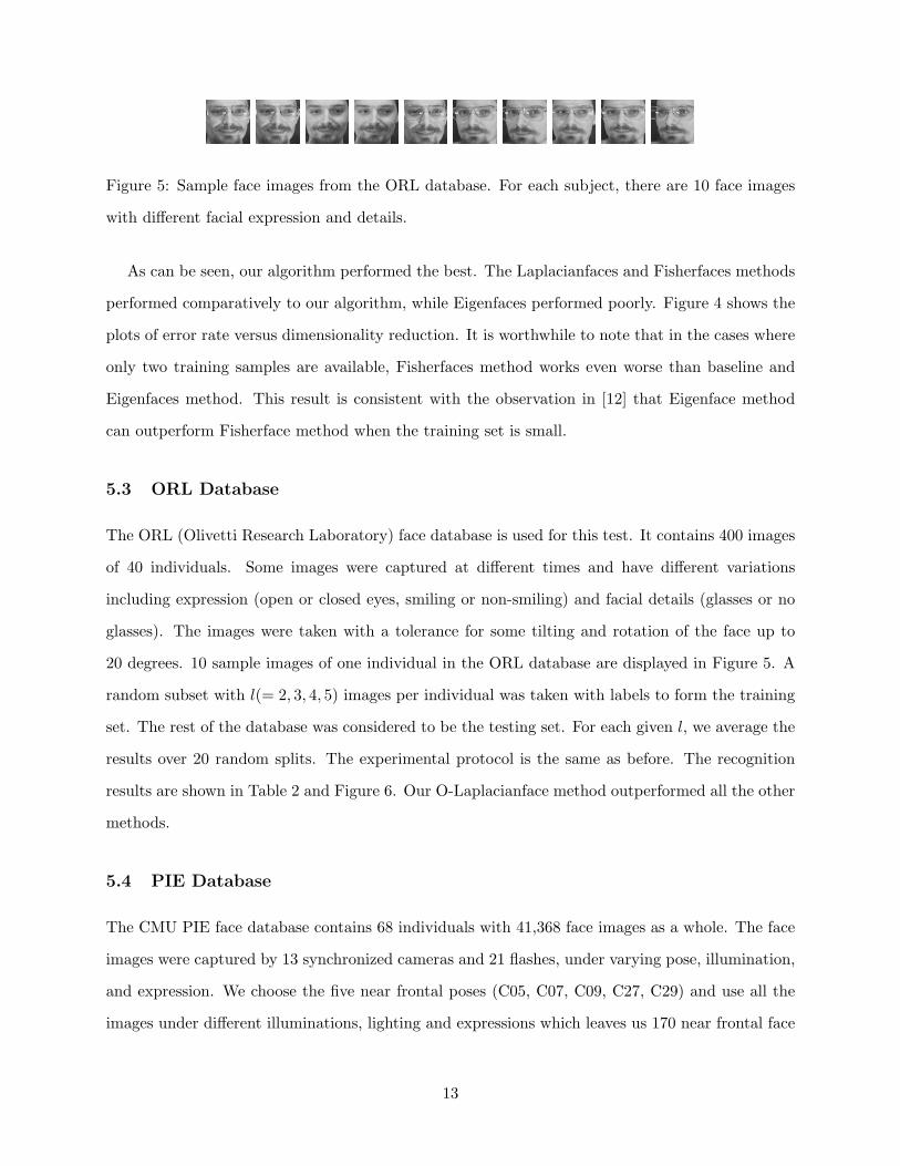
Figure 5: Sample face images from the ORL database. For each subject, there are 10 face images
with different facial expression and details.
As can be seen, our algorithm performed the best. The Laplacianfaces and Fisherfaces methods
performed comparatively to our algorithm, while Eigenfaces performed poorly. Figure 4 shows the
plots of error rate versus dimensionality reduction. It is worthwhile to note that in the cases where
only two training samples are available, Fisherfaces method works even worse than baseline and
Eigenfaces method. This result is consistent with the observation in [12] that Eigenface method
can outperform Fisherface method when the training set is small.
5.3 ORL Database
The ORL (Olivetti Research Laboratory) face database is used for this test. It contains 400 images
of 40 individuals. Some images were captured at different times and have different variations
including expression (open or closed eyes, smiling or non-smiling) and facial details (glasses or no
glasses). The images were taken with a tolerance for some tilting and rotation of the face up to
20 degrees. 10 sample images of one individual in the ORL database are displayed in Figure 5. A
random subset with l(= 2, 3, 4, 5) images per individual was taken with labels to form the training
set. The rest of the database was considered to be the testing set. For each given l, we average the
results over 20 random splits. The experimental protocol is the same as before. The recognition
results are shown in Table 2 and Figure 6. Our O-Laplacianface method outperformed all the other
methods.
5.4 PIE Database
The CMU PIE face database contains 68 individuals with 41,368 face images as a whole. The face
images were captured by 13 synchronized cameras and 21 flashes, under varying pose, illumination,
and expression. We choose the five near frontal poses (C05, C07, C09, C27, C29) and use all the
images under different illuminations, lighting and expressions which leaves us 170 near frontal face
13
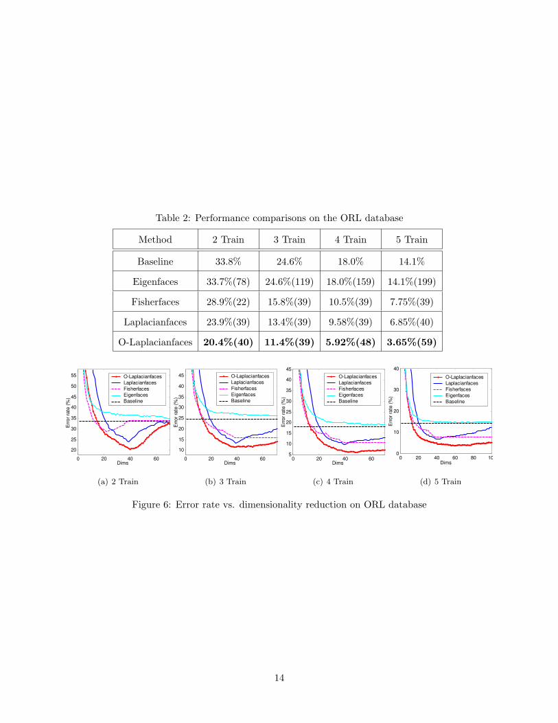
Table 2: Performance comparisons on the ORL database
Method 2 Train 3 Train 4 Train 5 Train
Baseline 33.8% 24.6% 18.0% 14.1%
Eigenfaces 33.7%(78) 24.6%(119) 18.0%(159) 14.1%(199)
Fisherfaces 28.9%(22) 15.8%(39) 10.5%(39) 7.75%(39)
Laplacianfaces 23.9%(39) 13.4%(39) 9.58%(39) 6.85%(40)
O-Laplacianfaces 20.4%(40) 11.4%(39) 5.92%(48) 3.65%(59)
0 20 40 60
20
25
30
35
40
45
50
55
Dims
Err
or
rate
(%
)
O-Laplacianfaces
Laplacianfaces
Fisherfaces
Eigenfaces
Baseline
(a) 2 Train
0 20 40 60
10
15
20
25
30
35
40
45
Dims
Err
or
rate
(%
)
O-Laplacianfaces
Laplacianfaces
Fisherfaces
Eigenfaces
Baseline
(b) 3 Train
0 20 40 605
10
15
20
25
30
35
40
45
Dims
Err
or
rate
(%
)
O-Laplacianfaces
Laplacianfaces
Fisherfaces
Eigenfaces
Baseline
(c) 4 Train
0 20 40 60 80 1000
10
20
30
40
Dims
Err
or
rate
(%
)
O-Laplacianfaces
Laplacianfaces
Fisherfaces
Eigenfaces
Baseline
(d) 5 Train
Figure 6: Error rate vs. dimensionality reduction on ORL database
14
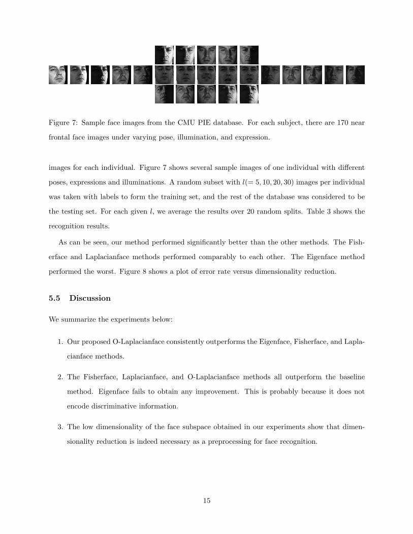
Figure 7: Sample face images from the CMU PIE database. For each subject, there are 170 near
frontal face images under varying pose, illumination, and expression.
images for each individual. Figure 7 shows several sample images of one individual with different
poses, expressions and illuminations. A random subset with l(= 5, 10, 20, 30) images per individual
was taken with labels to form the training set, and the rest of the database was considered to be
the testing set. For each given l, we average the results over 20 random splits. Table 3 shows the
recognition results.
As can be seen, our method performed significantly better than the other methods. The Fish-
erface and Laplacianface methods performed comparably to each other. The Eigenface method
performed the worst. Figure 8 shows a plot of error rate versus dimensionality reduction.
5.5 Discussion
We summarize the experiments below:
1. Our proposed O-Laplacianface consistently outperforms the Eigenface, Fisherface, and Lapla-
cianface methods.
2. The Fisherface, Laplacianface, and O-Laplacianface methods all outperform the baseline
method. Eigenface fails to obtain any improvement. This is probably because it does not
encode discriminative information.
3. The low dimensionality of the face subspace obtained in our experiments show that dimen-
sionality reduction is indeed necessary as a preprocessing for face recognition.
15
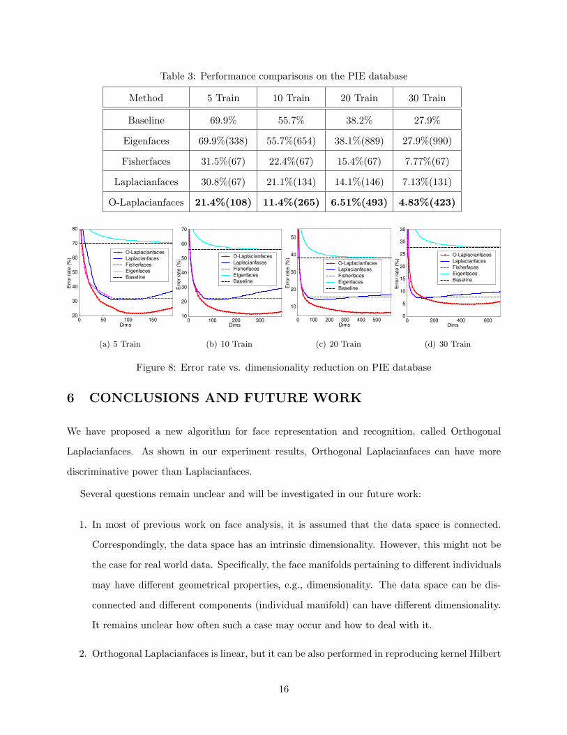
Table 3: Performance comparisons on the PIE database
Method 5 Train 10 Train 20 Train 30 Train
Baseline 69.9% 55.7% 38.2% 27.9%
Eigenfaces 69.9%(338) 55.7%(654) 38.1%(889) 27.9%(990)
Fisherfaces 31.5%(67) 22.4%(67) 15.4%(67) 7.77%(67)
Laplacianfaces 30.8%(67) 21.1%(134) 14.1%(146) 7.13%(131)
O-Laplacianfaces 21.4%(108) 11.4%(265) 6.51%(493) 4.83%(423)
0 50 100 15020
30
40
50
60
70
80
Dims
Err
or
rate
(%
)
O-Laplacianfaces
Laplacianfaces
Fisherfaces
Eigenfaces
Baseline
(a) 5 Train
0 100 200 30010
20
30
40
50
60
70
Dims
Err
or
rate
(%
)
O-Laplacianfaces
Laplacianfaces
Fisherfaces
Eigenfaces
Baseline
(b) 10 Train
0 100 200 300 400 500
10
20
30
40
50
Dims
Err
or
rate
(%
)
O-Laplacianfaces
Laplacianfaces
Fisherfaces
Eigenfaces
Baseline
(c) 20 Train
0 200 400 6000
5
10
15
20
25
30
35
Dims
Err
or
rate
(%
)
O-Laplacianfaces
Laplacianfaces
Fisherfaces
Eigenfaces
Baseline
(d) 30 Train
Figure 8: Error rate vs. dimensionality reduction on PIE database
6 CONCLUSIONS AND FUTURE WORK
We have proposed a new algorithm for face representation and recognition, called Orthogonal
Laplacianfaces. As shown in our experiment results, Orthogonal Laplacianfaces can have more
discriminative power than Laplacianfaces.
Several questions remain unclear and will be investigated in our future work:
1. In most of previous work on face analysis, it is assumed that the data space is connected.
Correspondingly, the data space has an intrinsic dimensionality. However, this might not be
the case for real world data. Specifically, the face manifolds pertaining to different individuals
may have different geometrical properties, e.g., dimensionality. The data space can be dis-
connected and different components (individual manifold) can have different dimensionality.
It remains unclear how often such a case may occur and how to deal with it.
2. Orthogonal Laplacianfaces is linear, but it can be also performed in reproducing kernel Hilbert
16
space which gives rise to nonlinear maps. The performance of OLPP in reproducing kernel
Hilbert space need to be further examined.
References
[1] A. U. Batur and M. H. Hayes. Linear subspace for illumination robust face recognition. In
IEEE Conference on Computer Vision and Pattern Recognition, 2001.
[2] P.N. Belhumeur, J.P. Hepanha, and D.J. Kriegman. Eigenfaces vs. fisherfaces: recognition us-
ing class specific linear projection. IEEE Trans. on Pattern Analysis and Machine Intelligence,
19(7):711–720, 1997.
[3] M. Belkin and P. Niyogi. Laplacian eigenmaps and spectral techniques for embedding and
clustering. In Advances in Neural Information Processing Systems 14, pages 585–591. MIT
Press, Cambridge, MA, 2001.
[4] Fan R. K. Chung. Spectral Graph Theory, volume 92 of Regional Conference Series in Math-
ematics. AMS, 1997.
[5] J. Duchene and S. Leclercq. An optimal transformation for discriminant and principal com-
ponent analysis. IEEE Trans. on PAMI, 10(6):978–983, 1988.
[6] R. O. Duda, P. E. Hart, and D. G. Stork. Pattern Classification. Wiley-Interscience, Hoboken,
NJ, 2nd edition, 2000.
[7] G. H. Golub and C. F. Van Loan. Matrix computations. Johns Hopkins University Press, 3rd
edition, 1996.
[8] R. Gross, J. Shi, and J. Cohn. Where to go with face recognition. In Third Workshop on
Empirical Evaluation Methods in Computer Vision, Kauai, Hawaii, December 2001.
[9] X. He, S. Yan, Y. Hu, P. Niyogi, and H.-J. Zhang. Face recognition using laplacianfaces. IEEE
Trans. on Pattern Analysis and Machine Intelligence, 27(3), 2005.
[10] Xiaofei He and Partha Niyogi. Locality preserving projections. In Advances in Neural Infor-
mation Processing Systems 16. MIT Press, Cambridge, MA, 2003.
17
[11] Q. Liu, R. Huang, H. Lu, and S. Ma. Face recognition using kernel based fisher discrimi-
nant analysis. In Proc. of the fifth International Conference on Automatic Face and Gesture
Recognition, Washington, D. C., May 2002.
[12] A. M. Martinez and A. C. Kak. PCA versus LDA. IEEE Trans. on PAMI, 23(2):228–233,
2001.
[13] B. Moghaddam and A. Pentland. Probabilistic visual learning for object representation. IEEE
Trans. on PAMI, 19(7):696–710, 1997.
[14] H. Murase and S. K. Nayar. Visual learning and recognition of 3-d objects from appearance.
International Journal of Computer Vision, 14, 1995.
[15] P. J. Phillips. Support vector machines applied to face recognition. Advances in Neural
Information Processing Systems, 11:803–809, 1998.
[16] S Roweis and L Saul. Nonlinear dimensionality reduction by locally linear embedding. Science,
290(5500):2323–2326, 2000.
[17] T. Shakunaga and K. Shigenari. Decomposed eigenface for face recognition under various
lighting conditions. In IEEE Conference on Computer Vision and Pattern Recognition, Hawaii,
December 2001.
[18] T. Sim, S. Baker, and M. Bsat. The CMU pose, illuminlation, and expression database. IEEE
Trans. on PAMI, 25(12):1615–1618, 2003.
[19] J. Tenenbaum, V. de Silva, and J. Langford. A global geometric framework for nonlinear
dimensionality reduction. Science, 290(5500):2319–2323, 2000.
[20] M. Turk and A. Pentland. Eigenfaces for recognition. Journal of Cognitive Neuroscience,
3(1):71–86, 1991.
[21] M. Turk and A. P. Pentland. Face recognition using eigenfaces. In IEEE Conference on
Computer Vision and Pattern Recognition, Maui, Hawaii, 1991.
18