ORIGINAL PAPER Jan Awrejcewicz Application and

Acta Mech 226, 2831–2848 (2015)DOI 10.1007/s00707-015-1353-z

ORIGINAL PAPER

Grzegorz Kudra · Jan Awrejcewicz

Application and experimental validation of newcomputational models of friction forces and rolling resistance

Received: 27 October 2014 / Published online: 14 April 2015© The Author(s) 2015. This article is published with open access at Springerlink.com

Abstract In the process of modelling of the Celtic stone rotating and rolling on a plane surface, differentversions of simplified models of contact forces between two contacting bodies are used. The consideredcontact models take into account coupled dry friction force and torque, as well as rolling resistance. Theywere developed using Padé approximations, their modifications, and polynomial functions. Before the use ofthese models, some kinds of regularisations have been made, allowing to avoid singularities in the differentialequations. The models were tested both numerically and experimentally, giving some practical guesses ofthe most essential elements of contact modelling in the Celtic stone numerical simulations. Since the testedcontact models do not require the space discretisation, they can find application in relatively fast numericalsimulations of rigid bodies with friction contacts.

1 Introduction

One can identify examples of mechanical systems with frictional contacts, such as billiard ball, Thompsontop, Celtic stone, electric polishing machine, rolling bearings, where an assumption of the point contact andone-dimensional friction model cannot lead to correct results. Moreover, the rolling resistance can play animportant role in such systems. The one possible approach is to solve the full problem of frictional contact ofdeformable bodies on a finite area by performing the discretisation in space and then application, for example,of the finite element method. However, this leads to a great increase in computational cost of the simulation.On the other hand, some applications (computer games, predictive control) can require more efficient modelsand faster simulations, less accurate but still mapping the most important properties of the real object. In suchcases, the good idea is to develop and use some kinds of simplified models of the resulting friction forces androlling resistance.

A literature survey shows that there were some attempts to develop approximate models of friction forcesand rolling resistance for a finite contact area suitable for relatively fast numerical simulation of rigid bodies.Contensou [7] assumed fully developed sliding and Coulomb friction law on some circular contact area withHertzian pressure distribution and then developed an integral model of the resultant friction force. The obtainedmodel of friction force is often referred to as Coulomb–Contensou friction model.

A group of researchers working in the field of robotics [11], assuming plane and non-deformable contactzone, proposed an ellipsoid as an approximation of limit surface, which bounds the area of admissible valuesof the components of friction force and moment. It is a relatively good approximation for the determination

G. Kudra (B) · J. AwrejcewiczDepartment of Automation, Biomechanics and Mechatronics (K16), Lodz University of Technology,1/15 Stefanowski St., 90-924 Lodz, PolandE-mail: [email protected].: +48-42-6312339Fax: +48-42-6312225

http://crossmark.crossref.org/dialog/?doi=10.1007/s00707-015-1353-z&domain=pdf

2832 G. Kudra, J. Awrejcewicz

of admissible loadings of the contact for which the developed sliding does not occur. For determination of thesliding direction, they used the properties of the convex zone of admissible loadings of the contact, i.e. the factthat its normal direction determines the components of sliding [9]. But in this case, the approximation by theuse of the ellipsoid leads to much higher errors.

Zhuravlev [30] developed essentially the results of Contensou for circular contact area with Coulombfriction law and fully developed sliding, by giving exact analytical expressions for friction force and moment.Since the obtained analytical results are not convenient in practical use, he also proposed the correspondingfirst-order Padé approximants as effective approximation of the integral model of friction [31]. For the same contact,the coupled friction model was approximated by the use of Taylor expansion of the velocity pseudo potential[21]. The same group of authors proposed for this contact an ellipse as an alternative efficient approximationof the relation between the magnitude of friction force and moment [27]. The piece-wise linear approximationof integral friction model for elliptic contact area and the Hertz stress distribution was presented in paper [15].Kireenkov [15] constructed the coupled model of friction forces and rolling resistance for circular contactarea with Coulomb friction law and fully developed sliding. He used the second-order Padé approximants,which are more accurate and suitable for qualitative analysis. The rolling resistance was modelled as a resultof distortion of initial Hertzian stress distribution.

In the work [19], the authors presented some generalisations and modifications of Padé approximantsand applied them in modelling of friction forces for fully developed sliding on circular contact area, withconstant contact pressure. The presented new family of models can be understood as a bridge between Padéapproximations and models proposed by Möller et al. [27]. The continuation of the project [19] is presented inwork [20], where an integral model of dry friction components is built for a general shape of plane contact area.Then, the special model of stress distribution over the elliptic contact patch is developed, being a generalisationof Hertzian distribution, with addition of special distortion related to the resistance of rolling. At the end, someapproximations of the resultant friction forces are exhibited, being piece-wise polynomial functions as well asfurther generalisations and developments of Padé approximants.

A good object for testing coupledmathematicalmodels of dry friction components and rolling resistance forelliptic contact area is the Celtic stone, also known as wobblestone or rattleback. It is usually a semi-ellipsoidalsolid (or another kind of body with a smoothly curved oblong lower surface) with a special mass distribution.Most celts lie on a flat horizontal surface and when set in rotational motion around the vertical axis can rotatein one direction only. The imposition of an initial spin in the opposite direction leads to transverse wobblingand then to spinning in the preferred direction.

The Celtic stone with its special dynamical properties was an object of investigation of many researchers,and the first scientific publication on this subject appeared at the end of the nineteenth century [28]. Dissipation-free rolling without slip is one of the widely used assumptions in modelling of the celt [4,5,23,28].Walker [28]pointed out the non-coincidence of the principal axes of inertia and the principal directions of curvature at theequilibrium contact point as essential in explanation of thewobblestone properties. An analysis of the linearisedequations of the model assuming continuous slipping (quasi-viscous relation between the friction force andvelocity of the contact point) is presented byMagnus [24]. Another model which takes into account dissipation,but is far from reality, is analysed using the asymptotic perturbation theory [6]. Some authors proposed amodel,which assumes rolling without slip and viscous damping (torque about all three axes) [13]. Garcia and Hubbard[8] presented a more realistic modelling with aerodynamic dissipation and slip with dry friction force. Theycompleted the model with an experimental validation. Markeev [25] performed the perturbation analysis oflocal dynamics around the equilibrium points of the model assuming the absence of friction. He also gave theexperimental verification. The modelling of celt closer to reality is proposed by Zhuravlev [32], who assumedthe possibility of slip, but in contrast to all the earlier works, applied the spatial Coulomb–Contensou frictionmodel with linear Padé approximations for circular contact patch [14,30,31]. However, since the frictionforce is the only way of dissipation in the proposed model, the time of the wobblestone motion (until rest) isunrealistically long.In the papers [16,17] there is presented an attempt to more realistic modelling of the Celtic stone dynamics,where both friction force and torque are taken into account, as well as rolling resistance. The Coulomb–Contensou model and the first-order Padé approximants are applied to model the frictional coupling betweentranslational and rotational motion of the circular contact area. The dependence of the dynamical responseon initial conditions and the system parameters is investigated, showing essential differences in the propertiesof the proposed model, when compared with the previous simulation models of the celt. The complete setof hyperbolic tangent functions approximating friction components coupled with rolling friction for circularcontact area is proposed and then applied in thewobblestone dynamicsmodelling in the work [18]. In theworks

Application and experimental validation of new computational models of friction 2833

[1,2], the series of the Celtic stonemodels, with different levels of complexity of themodel of the contact forcesfor the elliptic contact zone (from the independent friction force and torque components, to the second-orderPadé approximants), are investigated. The simulations are compared with the corresponding results obtainedby the use of the model, where the friction components of the integral model are approximated by moreprecise, but much more complicated approximations based on the piece-wise polynomials. The untypicallyforced wobblestone, i.e. situated on a harmonically vibrating base, is investigated numerically in the work [3],where rich bifurcation dynamics is detected and presented.

Section 2 of the present work is devoted to mathematical modelling of the Celtic stone as a rigid bodywith continuous contact with the plane surface. Section 3 presents the corresponding approximate coupledmodels of dry friction components (spatial force and torque), rolling resistance and their implementation inthe wobblestone model. Sections 3.1 and 3.2 are in fact a kind of an extract from the paper [20]. In Sect. 4 wepresent results of numerical and experimental investigations: parameter estimation results, analysis of differentversions of the contact model, comparisons between simulation and experimental solutions. Section 5 givessome final remarks.

2 Mathematical modelling of the wobblestone

2.1 Differential and algebraic equations of motion

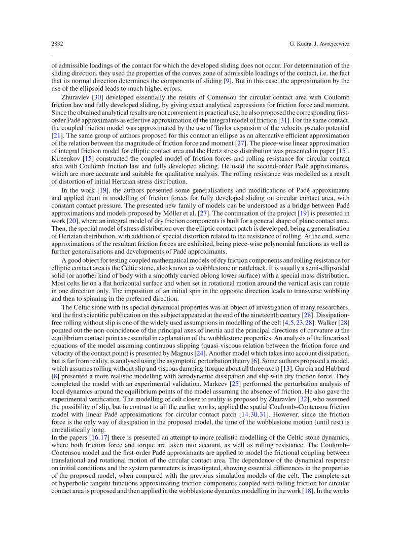
Thewobblestone as a semi-ellipsoid rigid bodywith the geometry centre O andmass centreC (with the relativeposition defined by vector k) touching a rigid, flat and immovable horizontal surface π (parallel to the X1X2plane of the global immovable coordinate system GX1X2X3) at point A is presented in Fig. 1 [1–3,16–18].

The differential equations of motion can be written as follows:

mdvdt

= −mgn + Nn + T(Zi )sε , (1)

drCdt

= v, (2)

Bdω

dt+ ω × (Bω) = (r + k) ×

(Nn + T(Zi )

sε

)+ M(Zi )

sε + M(Z)rε , (3)

ψ = ω3 cosϕ − ω1 sin ϕ

cos θ,

θ = ω1 cosϕ + ω3 sin ϕ,

ϕ = ω2 + tan θ (ω1 sin ϕ − ω3 cosϕ ) , (4)

wherem is the mass of the celt, B is the tensor of inertia of the solid in mass centreC , v is the absolute velocityof mass centre C , ω is the absolute angular velocity of the body, rC = rGC is the vector defining the positionof mass centre C with respect to the origin G of the global coordinate system, N = Nn is the normal reactionof the horizontal plane, n is the unit vector normal to the plane X1X2, T

(Zi )sε (ignored in Fig. 1) is the sliding

friction force in the point of contact A, M(Zi )sε and M(Z)

rε (ignored in Fig. 1) are the dry friction and rolling

Fig. 1 Wobblestone on a horizontal plane π with the coordinate systems


resistance torques applied to the body, respectively. The symbols Z = A, B,C, D, E and i = H, 1, 2, 3denote the version of the contact model (see the Sect. 3.2). Vector r indicates the actual position of the contactpoint A. Equation (1) represents the law of motion of the mass centre of the body in the absolute coordinatesystem, while Eq. (3) exhibits the law of variation of the angular momentum expressed in the local frame,where the notation du/dt stands for the time derivative of vector u in the movable body-fixed coordinatesystem. Equation (4) represents the relations between the components of ω in the local reference frame andderivatives of Cardan angles describing the orientation of the body by the following sequence of three rotationsabout the axes of the local coordinate system Cx1x2x3 (of axes parallel to the geometric axes of the ellipsoid):x3 (by an angle ψ), x1 (by an angle θ ) and x2 (by an angle ϕ).

For any vector u = ux1ex1 +ux2ex2 +ux3ex3 , where ex1 ex2 and ex3 are the unit vectors of the correspondingaxes of the local coordinate system Cx1x2x3, we use notations uxi = ui and exi = ei (i = 1, 2, 3). Moreover,we denote the components of inertia tensor B in the local reference frame as follows:

B =⎡⎣

B1 −B12 −B13−B12 B2 −B23−B13 −B23 B3

⎤⎦ (5)

where Bi = Bxi is the moment of inertia of the body with respect to axis Cxi (i = 1, 2, 3), while Bi j = Bxi x jis the corresponding centrifugal moment of inertia (i, j = 1, 2, 3 and i �= j).

Since the numerical simulations are performed in both the local and global reference frames, one needsthe following rule of transformation between the corresponding coordinates of a vector u:

[uX1 uX2 uX3

]T = BψBn[u1 u2 u3

]T (6)

where

Bψ =⎡⎣cosψ − sinψ 0sinψ cosψ 00 0 1

⎤⎦ , Bn =

⎡⎣

cosϕ 0 sin ϕsin ϕ sin θ cos θ − cosϕ sin θ

− sin ϕ cos θ sin θ cosϕ cos θ

⎤⎦ . (7)

Applying the above transformation to the coordinates of vector n, we get⎧⎨⎩n1n2n3

⎫⎬⎭ = B−1

n B−1ψ

⎧⎨⎩001

⎫⎬⎭ =

⎧⎨⎩

− sin ϕ cos θsin θ

cosϕ cos θ

⎫⎬⎭ . (8)

In order to find the relation between vectors r and n, one can use the following ellipsoid equation:

φ (r) = r21a21

+ r22a22

+ r23a23

− 1 = 0 (9)

(where a1, a2 and a3 are the semi-axes of the ellipsoid along the axes x1, x2 and x3, respectively) and thecondition of tangent contact between the ellipsoid and horizontal plane

n = δdφ

dr, (10)

where δ < 0. The solution to Eqs. (9) and (10) with respect to the components of r and δ in the Cx1x2x3coordinate system reads

r1 = a21n12δ

, r2 = a22n22δ

, r3 = a23n32δ

, (11)

where

δ = −1

2

√a21n

21 + a22n

22 + a23n

23. (12)

The set of Eqs. (1)–(4) consists of 12 scalar first-order ordinary differential equations with 13 unknownfunctions of time: vX1 , vX2 , vX3 , rCX1 , rCX2 , rCX3 , ω1, ω2, ω3, ψ , θ , ϕ and N . The missing equation is thefollowing algebraic expression:

(rC + r + k) · n = 0, (13)


which follows from the fact that the point A always lies in the plane π . Equations (1)–(4) and (13) form nowthe set of differential–algebraic equations of index 3.

Differentiating the condition (13) with respect to time in the global coordinate system GX1X2X3, one gets

d

dt(rC + r + k) · n + (rC + r + k) · dn

dt= 0. (14)

Sinced

dt(rC + r + k) = drC

dt+ d

dt(r + k) + ω × (r + k) , (15)

drC/dt = v, dk/dt = 0 and (dr/dt) · n = 0, Eq. (14) takes the following form:

[v + ω × (r + k)] · n = 0, (16)

which expresses the fact that velocity vA = v + ω × (r + k) lies in the plane π . Equations (1)–(4) and (16)are now the differential–algebraic equations of index 2.

Differentiating the algebraic condition again, one obtains

d

dt(v + ω × (r + k)) · n + (v + ω × (r + k)) · dn

dt= 0. (17)

Sinced

dt(v + ω × (r + k))

dvdt

+ d

dt(ω × (r + k)) + ω × (ω × (r + k))

= dvdt

+ dω

dt× (r + k) + ω ×

(drdt

+ dkdt

)+ ω × (ω × (r + k)) ,

(18)

we finally get the following differential equation:[dvdt

+ dω

dt× (r + k) + ω × dr

dt+ ω × (ω × (r + k))

]· n = 0. (19)

Since in the above expressions the local derivatives of vector r appear, one need to differentiate the expressions(11) with respect to time and then do the same with the local components (8) of vector n.

Now we have the set (1)–(4) and (19) of 13 scalar differential–algebraic equations of index 1, with 13unknown functions of time, but with only 12 derivatives of unknown functions. One can solve themwith respectto the corresponding derivatives and the normal reaction N and obtain the set of 12 differential equations with12 unknown functions. During numerical simulations of the Celtic stone, one should be very careful whenchoosing the numerical method and initial conditions, since, especially during the long time simulations, thereis a risk of violation of two algebraic conditions (13) and (16).

Note that we have chosen the local coordinate system with the axes parallel to the geometric axes ofthe ellipsoid, instead of central and principal axes of inertia. In the second case the tensor of inertia takesa convenient form of diagonal matrix. However this advantage is lost since the unknown N appears in theright-hand side of Eq. (3) (note that function N appears also in the expressions for T(Zi )

sε , M(Zi )sε and M(Z)

rε ).Moreover, the relation between the vectors r and n is simpler in the chosen coordinate system Cx1x2x3.

2.2 Principal curvatures of the ellipsoid

For some developed later contact models we will take into account time variation of the curvatures of thewobblestone surface in the point of contact with the base. While limiting considerations to the surface ofrevolution, the following parametric description of the wobblestone surface can be proposed:

r1 (p, q) = α (p) ,

r2 (p, q) = β (p) cos q,

r3 (p, q) = β (p) sin q (20)


whereα (p) = a1 cos p, β (p) = a2 sin p, (21)

for parameters 0 ≤ p ≤ π and 0 ≤ q < 2π .Now the principal curvatures can be expressed as follows [10]:

κ1 = sgn (β)(β ′′α′ − β ′α′′)

(β ′2 + α′2)3/2 , κ2 = − α′

|β| (β ′2 + α′2)1/2 (22)

where κ1 = R−11 is the curvature in the meridional direction (in the section including the Ox1 axis), whereas

κ2 = R−12 is the curvature in the corresponding transverse direction (R1 and R2 are the corresponding curvature

radii).From Eqs. (22) and (21) we get

κ1 = a1a2(a21 − (

a21 − a22)cos2 p

)3/2 , κ2 = a1

a2(a21 − (

a21 − a22)cos2 p

)1/2 . (23)

Equations (20)–(21) give the relationr21a21

= cos2 p, (24)

which leads to the following form of Eqs. (23):

κ1 = a1a2(a21 − a21−a22

a21r21

)3/2 , κ2 = a1

a2

(a21 − a21−a22

a21r21

)1/2 .(25)

The curvature ratio of ellipsoid κ = κ2/κ1 reads

κ = a21a22

+ r21a21

− r21a22

(26)

where κ > 1 for a1 > a2 and −a1 < r1 < a1. In the case of the contact between the Celtic stone with theplane surface, the principal curvatures and the corresponding principal directions of the ellipsoid surface arealso the relative principal curvature and relative principal directions of the contact.

As mentioned in the Sect. 1, the non-coincidence of the principal directions of curvature and the principalaxes of inertia at the equilibrium contact point is responsible for the typical dynamical properties of the Celticstone. This can be realised in the two ways: (i) an asymmetrical base of the stone with the skewed principaldirections of curvature and (ii) a symmetrical base, but special mass distribution is obtained by the use ofadditional elements mounted on the stone. Since we assume a geometry of the body in the form of an ellipsoid,the wobblestone investigated in this work is of the second kind.

3 Friction and rolling resistance modelling

3.1 Contact pressure distribution, rolling resistance and integral model of friction forces

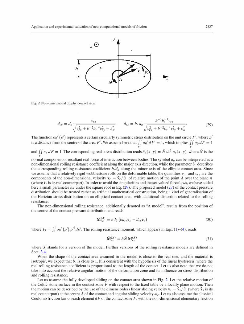
Figure 2 exhibits the non-dimensional elliptic contact area F with the co-ordinate system Axy, where thevector n faces the wobblestone. The real co-ordinates of any point are x = ax and y = a y, where a is the reallength of the major semi-axis of the elliptic contact.

Based on the work [20], we assume the following non-dimensional distribution of the contact pressurebetween the Celtic stone and the base plane:

σε(x, y) = σ0 (x, y)(1 + dcεx + b−1dsε y

)(27)

where

σ0(x, y) = b−1σ0′(√

x2 + b−2y2)

, (28)


Fig. 2 Non-dimensional elliptic contact area

dcε = davr x√

v2r x + b−2b−2r v2ry + ε2R

, dsε = br dab−1b−1

1 vry√v2r x + b−2b−2

r v2ry + ε2R

. (29)

The function σ0′ (ρ′) represents a certain circularly symmetric stress distribution on the unit circle F ′, where ρ′

is a distance from the centre of the area F ′. We assume here that∫∫F ′

σ0′ dF ′ = 1, which implies

∫∫F

σ0 dF = 1

and∫∫F

σε dF = 1. The corresponding real stress distribution reads σε(x, y) = N/a2 σε(x, y), where N is the

normal component of resultant real force of interaction between bodies. The symbol da can be interpreted as anon-dimensional rolling resistance coefficient along the major axis direction, while the parameter br describesthe corresponding rolling resistance coefficient brda along the minor axis of the elliptic contact area. Sincewe assume that a relatively rigid wobblestone rolls on the deformable table, the quantities vr x and vry are thecomponents of the non-dimensional velocity vr = vr/ a of relative motion of the point A over the plane π(where vr is its real counterpart). In order to avoid the singularities and the set-valued force laws, we have addedhere a small parameter εR under the square root in Eq. (29). The proposed model (27) of the contact pressuredistribution should be treated rather as artificial mathematical construction, being a kind of generalisation ofthe Hertzian stress distribution on an elliptical contact area, with additional distortion related to the rollingresistance.

The non-dimensional rolling resistance, additionally denoted as “A model”, results from the position ofthe centre of the contact pressure distribution and reads

M(A)rε = π I3

(bdsεex − dcεey

)(30)

where I3 = ∫ 10 σ0

′ (ρ′) ρ′3dρ′. The rolling resistance moment, which appears in Eqs. (1)–(4), reads

M(X)rε = a N M(X)

rε (31)

where X stands for a version of the model. Further versions of the rolling resistance models are defined inSect. 3.4.

When the shape of the contact area assumed in the model is close to the real one, and the material isisotropic, we expect that br is close to 1. It is consistent with the hypothesis of the linear hysteresis, where thereal rolling resistance coefficient is proportional to the length of the contact. Let us also note that we do nottake into account the relative angular motion of the deformation zone and its influence on stress distributionand rolling resistance.

Let us assume the fully developed sliding on the contact area shown in Fig. 2. Let the relative motion ofthe Celtic stone surface in the contact zone F with respect to the fixed table be a locally plane motion. Thenthe motion can be described by the use of the dimensionless linear sliding velocity vs = vs/ a (where vs is itsreal counterpart) at the centre A of the contact and angular sliding velocity ωs . Let us also assume the classicalCoulomb friction law on each element dF of the contact zone F , with the non-dimensional elementary friction


force dTs = dTs/(μN ) acting on the celt, and its moment dMs = dMs/(a μN ) with respect to the pole A,where dTs is the real elementary force, dMs—the corresponding real moment andμ—dry friction coefficient.Assuming the resultant friction force and torque as Ts = −Tsxex − Ts yey andMs = −Msn, one gets

Tsx (vs, ωs, ϕs) =∫∫

F

σε(x, y)vs cosϕs − ωs y√

(vs cosϕs − ωs y)2 + (vs sin ϕs + ωs x)2dxdy,

Ts y (vs, ωs, ϕs) =∫∫

F

σε(x, y)vs sin ϕs + ωs x√

(vs cosϕs − ωs y)2 + (vs sin ϕs + ωs x)2dxdy,

Ms (vs, ωs, ϕs) =∫∫

F

σε(x, y)ωs

(x2 + y2

) + vs sin ϕs xs − vs cosϕs y√(vs cosϕs − ωs y)2 + (vs sin ϕs + ωs x)2

dxdy.

(32)

In Eq. (32) vs denotes the magnitude of the sliding velocity vs , while ωs is the projection of the vector ωs onthe vector n.

3.2 Approximate models of friction forces

In this section we present a series of different models approximating the integral model of friction (32), forthe contact pressure distribution (27), which do not require the space discretisation during the simulation ofthe wobblestone. All the exhibited models derive from those presented in the work [20], but in order to avoidthe singularities and the set-valued friction laws, they are additionally smoothed by means of introduction ofa small numerical parameter εT . In general, we can write

T(Xi )sε = −μN

(T (Xi )sεx ex + T (Xi )

sεy ey)

,

M(Xi )sε = −μN aM (Xi )

sε n (33)

where Xi stands for a specific version of the contact model.The simplest approximation to be tested, denoted as A0, is one ignoring the coupling between friction force

and torque,

T (A0)sxε = vsx

vsε, T (A0)

syε = vsy

vsε, M (A0)

sε = ωs

ωsε, (34)

where

vsε =√

v2s + ε2T , ωsε =√

ω2s + ε2T , (35)

and where vs x and vs y are components of the vector vs = vs xex + vs yey along the corresponding axes.

3.2.1 Generalisations of Padé approximants

In the work [20] the following approximation of the integral model (32) was proposed:

f (In) =∑n

i=0 a f,ivn−is ωi

s(vs

m f n + bm ff |ωs |m f n

)m−1 , (36)

for f = Tsx , Tsy, Ms , which can be understood as a kind of generalisation of a certain type of the Padéapproximants. The coefficients a f,i = a f,i (ϕs, sgn(ωs)) can be found from the following conditions:

∂ i f (In)

∂vis

∣∣∣∣∣vs=0

= ∂ f

∂vs

∣∣∣∣vs=0

,∂ i f (In)

∂ωis

∣∣∣∣∣ωs=0

= ∂ f

∂ωs

∣∣∣∣ωs=0

, (37)

for i = 0, ..., n1, where f = Tsx , Tsy, Ms .


Here we propose the following regularised version of the approximation (36):

f (In)ε =

∑ni=0 a fε,iv

n−isε ωi

s(vsε

m f n + bm ff |ωs |m f n

)m−1 , (38)

for f = Tsx , Tsy, Ms , where the variable vs has been replaced by the quantity vsε, defined by Eq. (35).The coefficients a f,i = a f,i (ϕs, sgn(ωs)) of the approximation (36) are functions of cos(ϕs) = vsx/vs andsin(ϕs) = vsy/vs . In the regularised version (38) of the model, they are replaced by the expressions vsx/vsεand vsy/vsε , correspondingly. Finally the coefficients a f,i are replaced by the functions a fε,i . The components

f (In)ε of the friction model (38) fulfil the conditions (37) for εT = 0.For n = 1 and n1 = 0 we get the following model:

T (A1)sxε = T (I1)

sxε = vsx − 4bTs bG (e) I2dsεωs(vmTssε + b

mTsTs

|ωs |mTs

)m−1Ts

,

T (A1)syε = T (I1)

syε = vsy + 4bTs H (e) I2dcεωs(vmTssε + b

mTsTs

|ωs |mTs

)m−1Ts

,

M (A1)sε = M (I1)

sε = 4bMs E (e) I2ωs + π I3(dcεvsy − bdsεvsx

)(bmMsMs

|ωs |mMs + vmMssε

)m−1Ms

,

(39)

while for n = 3 and n1 = 1 we have

T (A2)sxε = T (I3)

sxε

= v2sεvsx + ωs(bTs (4G(e)I0vsxωs − bdsε(π I3v2sy + 4G(e)I2ω2s )) − π I3dcεvsxvsy)

(v3mTssε + b

mTsTs

|ωs |3mTs )m−1

Ts

,

T (A2)syε = T (I3)

syε

= v2sεvsy + ωs(bTs (4H(e)I0vsyωs + dcε(π I3v2sx + 4H(e)I2ω2s )) + πbI3dsεvsxvsy)

(v3mTssε + b

mTsTs

|ωs |3mTs )m−1

Ts

,

M (A2)sε = M (I3)

sε

= 4bMsE(e)I2ω3

s + π I3((v2sx + b2v2sy)ωs + v2sε(dcεvsy − bdsεvsx ))

(bmMsMs

|ωs |3mMs + v3mMssε )

m−1Ms

(40)

where one has assumed that mTsx = mTsy = mTs and bTsx = bTsy = bTs .In Eqs. (39)–(40), the parameters and functions defined in the following way have been used:

Ii =∫ 1

0σ0

′ (ρ′) ρ′i dρ′,

G (e) = (K (e) − E (e)) e−2,

H (e) = (E (e) + (

e2 − 1)K (e)

)e−2 (41)

where K (e) and E(e) are the complete elliptic integrals of the first and second kind, while e = √1 − b2 is the

eccentricity of the contact. For numerical evaluation of the elliptic integrals during the simulation process seeRefs. [20,26].

Assuming the general case of the model of the contact pressure distribution presented in Sect. 3.1, all theparameters (b, I0, I2, I3, mTs , bTs , mMs , bMs , br and da) occurring in the non-dimensional models of frictionforces (39)–(40) (see also (29)) will be identified in Sect. 4 from the experimental data.


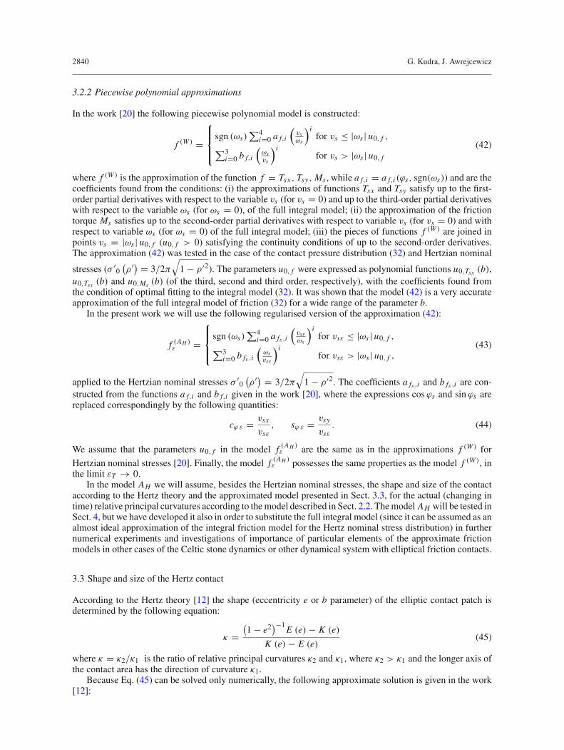
3.2.2 Piecewise polynomial approximations

In the work [20] the following piecewise polynomial model is constructed:

f (W ) =

⎧⎪⎨⎪⎩sgn (ωs)

∑4i=0 a f,i

(vsωs

)ifor vs ≤ |ωs | u0, f ,

∑3i=0 b f,i

(ωsvs

)ifor vs > |ωs | u0, f

(42)

where f (W ) is the approximation of the function f = Tsx , Tsy, Ms , while a f,i = a f,i (ϕs, sgn(ωs)) and are thecoefficients found from the conditions: (i) the approximations of functions Tsx and Tsy satisfy up to the first-order partial derivatives with respect to the variable vs (for vs = 0) and up to the third-order partial derivativeswith respect to the variable ωs (for ωs = 0), of the full integral model; (ii) the approximation of the frictiontorque Ms satisfies up to the second-order partial derivatives with respect to variable vs (for vs = 0) and withrespect to variable ωs (for ωs = 0) of the full integral model; (iii) the pieces of functions f (W ) are joined inpoints vs = |ωs | u0, f (u0, f > 0) satisfying the continuity conditions of up to the second-order derivatives.The approximation (42) was tested in the case of the contact pressure distribution (32) and Hertzian nominal

stresses (σ ′0(ρ′) = 3/2π

√1 − ρ′2). The parameters u0, f were expressed as polynomial functions u0,Tsx (b),

u0,Tsy (b) and u0,Ms (b) (of the third, second and third order, respectively), with the coefficients found fromthe condition of optimal fitting to the integral model (32). It was shown that the model (42) is a very accurateapproximation of the full integral model of friction (32) for a wide range of the parameter b.

In the present work we will use the following regularised version of the approximation (42):

f (AH )ε =

⎧⎪⎨⎪⎩sgn (ωs)

∑4i=0 a fε,i

(vsεωs

)ifor vsε ≤ |ωs | u0, f ,

∑3i=0 b fε,i

(ωsvsε

)ifor vsε > |ωs | u0, f ,

(43)

applied to the Hertzian nominal stresses σ ′0(ρ′) = 3/2π

√1 − ρ′2. The coefficients a fε,i and b fε,i are con-

structed from the functions a f,i and b f,i given in the work [20], where the expressions cosϕs and sin ϕs arereplaced correspondingly by the following quantities:

cϕ ε = vsx

vsε, sϕ ε = vsy

vsε. (44)

We assume that the parameters u0, f in the model f (AH )ε are the same as in the approximations f (W ) for

Hertzian nominal stresses [20]. Finally, the model f (AH )ε possesses the same properties as the model f (W ), in

the limit εT → 0.In the model AH we will assume, besides the Hertzian nominal stresses, the shape and size of the contact

according to the Hertz theory and the approximated model presented in Sect. 3.3, for the actual (changing intime) relative principal curvatures according to themodel described in Sect. 2.2. Themodel AH will be tested inSect. 4, but we have developed it also in order to substitute the full integral model (since it can be assumed as analmost ideal approximation of the integral friction model for the Hertz nominal stress distribution) in furthernumerical experiments and investigations of importance of particular elements of the approximate frictionmodels in other cases of the Celtic stone dynamics or other dynamical system with elliptical friction contacts.

3.3 Shape and size of the Hertz contact

According to the Hertz theory [12] the shape (eccentricity e or b parameter) of the elliptic contact patch isdetermined by the following equation:

κ =(1 − e2

)−1E (e) − K (e)

K (e) − E (e)(45)

where κ = κ2/κ1 is the ratio of relative principal curvatures κ2 and κ1, where κ2 > κ1 and the longer axis ofthe contact area has the direction of curvature κ1.

Because Eq. (45) can be solved only numerically, the following approximate solution is given in the work[12]:


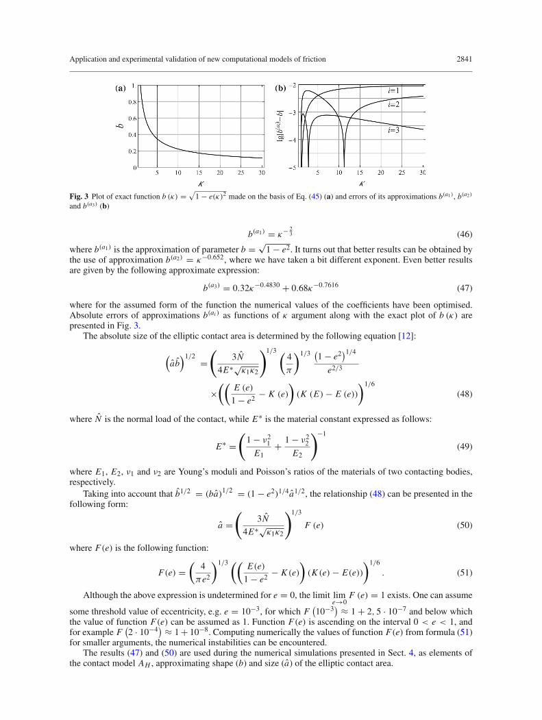
Fig. 3 Plot of exact function b (κ) =√1 − e(κ)2 made on the basis of Eq. (45) (a) and errors of its approximations b(a1), b(a2)

and b(a3) (b)

b(a1) = κ− 23 (46)

where b(a1) is the approximation of parameter b = √1 − e2. It turns out that better results can be obtained by

the use of approximation b(a2) = κ−0.652, where we have taken a bit different exponent. Even better resultsare given by the following approximate expression:

b(a3) = 0.32κ−0.4830 + 0.68κ−0.7616 (47)

where for the assumed form of the function the numerical values of the coefficients have been optimised.Absolute errors of approximations b(ai ) as functions of κ argument along with the exact plot of b (κ) arepresented in Fig. 3.

The absolute size of the elliptic contact area is determined by the following equation [12]:

(ab

)1/2 =(

3N

4E∗√κ1κ2

)1/3 (4

π

)1/3 (1 − e2

)1/4e2/3

×((

E (e)

1 − e2− K (e)

)(K (E) − E (e))

)1/6

(48)

where N is the normal load of the contact, while E∗ is the material constant expressed as follows:

E∗ =(1 − ν21

E1+ 1 − ν22

E2

)−1

(49)

where E1, E2, ν1 and ν2 are Young’s moduli and Poisson’s ratios of the materials of two contacting bodies,respectively.

Taking into account that b1/2 = (ba)1/2 = (1 − e2)1/4a1/2, the relationship (48) can be presented in the

following form:

a =(

3N

4E∗√κ1κ2

)1/3

F (e) (50)

where F(e) is the following function:

F(e) =(

4

πe2

)1/3 ((E(e)

1 − e2− K (e)

)(K (e) − E(e))

)1/6

. (51)

Although the above expression is undetermined for e = 0, the limit lime→0

F (e) = 1 exists. One can assume

some threshold value of eccentricity, e.g. e = 10−3, for which F(10−3

) ≈ 1 + 2, 5 · 10−7 and below whichthe value of function F(e) can be assumed as 1. Function F(e) is ascending on the interval 0 < e < 1, andfor example F

(2 · 10−4

) ≈ 1+ 10−8. Computing numerically the values of function F(e) from formula (51)for smaller arguments, the numerical instabilities can be encountered.

The results (47) and (50) are used during the numerical simulations presented in Sect. 4, as elements ofthe contact model AH , approximating shape (b) and size (a) of the elliptic contact area.


3.4 Implementation of the contact forces models

In order to apply the developed models of the resultant friction forces and rolling resistance in the numericalsimulations of the wobblestone mathematically modelled in Sect. 2, we need some relations between thecorresponding coordinate systems and vectors.

The versors of the coordinate system fixed to the contact patch are defined in the following way:

ex = e1π‖e1π‖ , ey = n × ex (52)

wheree1π = e1 − (e1 · n) n (53)

is the projection of versor e1 of the axis x1 onto the plane π (cf. Fig. 1). Here, we make an assumption that theaxis x1 is never perpendicular to plane π .

The non-dimensional sliding, spinning and rolling velocities are given by the following relations:

vs = vAa , ωs = ω · n,

vr = vs + vrc, vrc = drdt /a

(54)

where vA = v+ω × (r + k), vr is the relative velocity of the contact point (deformation region) over plane π(we assume that a relatively rigid wobblestone rolls on the deformable table) and vrc is the relative velocity ofdeformation region over the stone. Let us note that vrc can also be computed as vrc = (ω2κ

−11 e1−ω1κ

−12 e2)/a.

The corresponding components of the velocities are then determined as follows:

vsx = vs · ex , vsy = vs · ey,vr x = vr · ex , vry = vr · ey, i = 1, 2. (55)

In Sects. 3.1–3.3 we have defined the contact models A (rolling resistance), A0, A1, A2 and AH (frictionforces). Now we introduce the following further definitions of the model versions:

f (Bi )ε = f (Ai )

ε

∣∣∣m f =1

, for f = Tsx , Tsy, Ms,

M(B)rε = M(A)

rε ,

f (Ci )ε = f (Ai )

ε

∣∣∣b=1


M(C)rε = M(A)

rε

∣∣∣b=1

,

f (Di )ε = f (Ai )

ε

∣∣∣da=0


M(D)rε = M(A)

rε ,

f (Ei )ε = f (Ai )

ε

∣∣∣b=br=1

, for f = Tsx , Tsy, Ms

M(E)rε = M(A)

rε

∣∣∣b=br=1

,

(56)

where i = 1, 2 (we exclude the f (AH )ε model from the above definitions). Inmodels B we assume the parameter

m f equal to the one in all approximations of Padé type. Models C make an assumption of circular contactarea, but with an orthotropic rolling resistance kept. In models D we neglect the coupling between rollingresistance and friction force and torque, since the normal stress distribution is not distorted, but the rollingresistance model is preserved. In models E the contact area is circular and rolling resistance is isotropic.

In the case of the model AH , the Hertz nominal stress distribution (σ ′0(ρ′) = 3/2π

√1 − ρ′2) over the

elliptic contact area of size and shape according to the models presented in Sects. 2.2 and 3.3 is assumed. Theother models assume constant elliptic shape and size of the contact area during the motion of the celt, but anon-Hertzian, general case of the contact pressure distribution developed in Sect. 3.1.


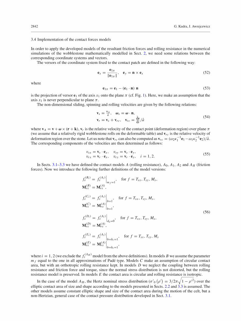
Fig. 4 Experimental model of the Celtic stone

4 Numerical and experimental investigations

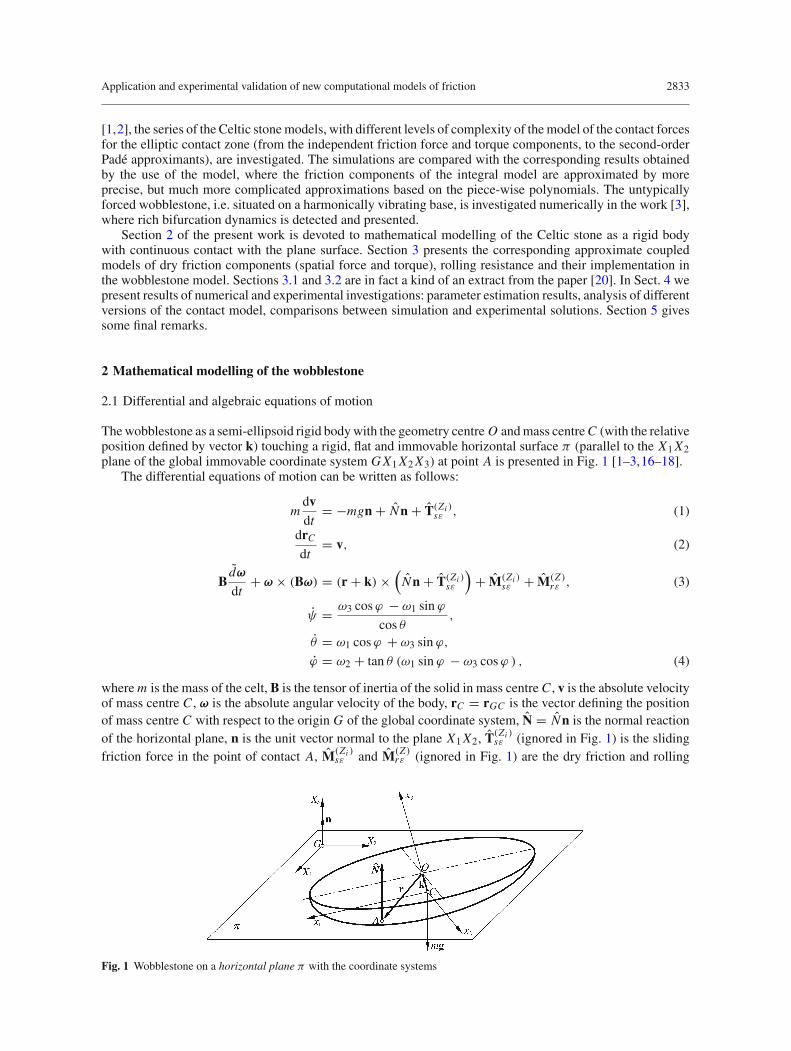
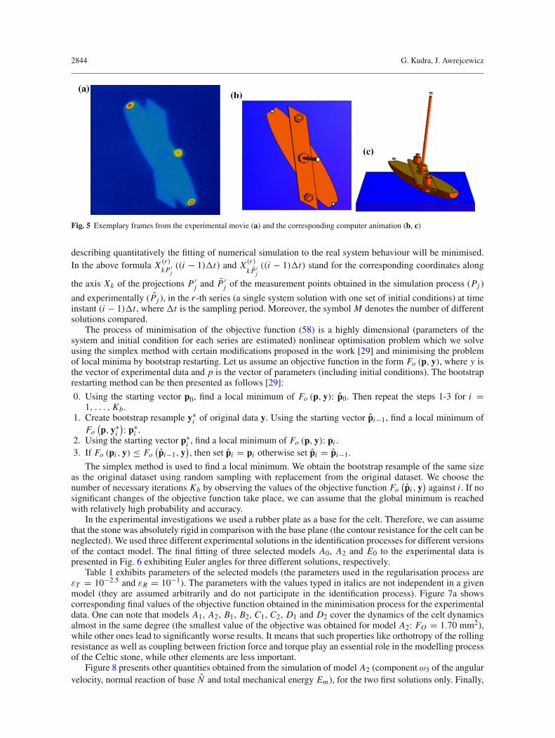
Figure 4 exhibits a photograph of the experimental model of the Celtic stone used in our investigations.The model was constructed by skew attachment of aluminium rod 2 to the semi-ellipsoidal body 1 made ofaluminium alloy EN AW-2017A. By the use of adjustment of the angle between axes of the rod and semi-ellipsoid, one could influence the product of inertia B12. Additional masses 3a and 3b made parameter B12larger. Three small steel elements 5, isolated from the celt thermally and playing the role ofmeasurement points,were placed on the stone. They were heated up before the experiment and then observed by a thermovisionvideo camera. Point P3 was located on top of rod 4 attached to the stone in such a way that it coincided withthe x3 axis of the local reference frame exhibited in Fig. 1.

The Celtic stone used in the experiment had the following parameters (acquired by the use of length andmass measurements as well as numerical integrations over the corresponding volumes): a1 = 110± 0.01mm,a2 = 25 ± 0.01mm, a3 = 25 ± 0.01mm, m = (543.6 ± 0.2) · 10−3 kg, B1 = 247.4 ± 1kg·mm2, B2 =1358.9± 1kg·mm2, B3 = 1374.7± 1 kg·mm2, B12 = 159.1± 1 kg·mm2, B13 = 0± 1 kg·mm2, B23 = 0± 1kg·mm2, k1 = 0 ± 0.1 mm, k2 = 0 ± 0.1 mm, k3 = 4.46 ± 0.1 mm.

The measurements were performed using a single thermovision video camera of 100Hz frequency and120 × 160 definition, located at a certain height above the stone with the axis of lens perpendicular to theplane base. The absolute position of the stone was determined uniquely (assuming the permanent contactbetween the stone and the base) by the coordinates of three points P1, P2 and P3 observed in the cameraimage. The coordinates of the measurement points in the local body-fixed reference frame were rOP11 =−97 ± 0.5 mm, rOP12 = 0 ± 0.5 mm, rOP13 = 4 ± 0.5mm, rOP21 = 97 ± 0.5 mm, rOP22 = 0 ± 0.5mm,rOP23 = 4 ± 0.5mm, rOP31 = 0 ± 0.5mm, rOP32 = 0 ± 0.5mm, rOP33 = 151 ± 0.5mm. Figure 5 shows anexemplary frame from the experimental movie compared to the corresponding one obtained from animationbased on the numerical simulation.

In order to compare the positions of points P1, P2 and P3 obtained from numerical simulations to thecorresponding experimental locations, we express the corresponding absolute positions of the points in thefollowing way:

rGPi = rPi = rC + k + rOPi , i = 1, 2, 3. (57)

Then they are projected centrally, with the centre at the focal point of the camera, onto the plane π .During the process of estimation of the parameters and initial conditions, the following objective function:

Fo = 1

6

M∑r=1

Nr

M∑r=1

Nr∑i=1

3∑j=1

2∑k=1

(X (r)kP ′

j((i − 1)�t)+ X (r)

k P ′j((i − 1)�t)

)2

(58)


Fig. 5 Exemplary frames from the experimental movie (a) and the corresponding computer animation (b, c)

describing quantitatively the fitting of numerical simulation to the real system behaviour will be minimised.In the above formula X (r)

kP ′j((i − 1)�t) and X (r)

k P ′j((i − 1)�t) stand for the corresponding coordinates along

the axis Xk of the projections P ′j and P ′

j of the measurement points obtained in the simulation process (Pj )

and experimentally (Pj ), in the r -th series (a single system solution with one set of initial conditions) at timeinstant (i − 1)�t , where �t is the sampling period. Moreover, the symbol M denotes the number of differentsolutions compared.

The process of minimisation of the objective function (58) is a highly dimensional (parameters of thesystem and initial condition for each series are estimated) nonlinear optimisation problem which we solveusing the simplex method with certain modifications proposed in the work [29] and minimising the problemof local minima by bootstrap restarting. Let us assume an objective function in the form Fo (p, y), where y isthe vector of experimental data and p is the vector of parameters (including initial conditions). The bootstraprestarting method can be then presented as follows [29]:

0. Using the starting vector p0, find a local minimum of Fo (p, y): p0. Then repeat the steps 1-3 for i =1, . . . , Kb.

1. Create bootstrap resample y∗i of original data y. Using the starting vector pi−1, find a local minimum of

Fo(p, y∗

i

): p∗

i .2. Using the starting vector p∗

i , find a local minimum of Fo (p, y): pi .3. If Fo (pi , y) ≤ Fo

(pi−1, y

), then set pi = pi otherwise set pi = pi−1.

The simplex method is used to find a local minimum. We obtain the bootstrap resample of the same sizeas the original dataset using random sampling with replacement from the original dataset. We choose thenumber of necessary iterations Kb by observing the values of the objective function Fo

(pi , y

)against i . If no

significant changes of the objective function take place, we can assume that the global minimum is reachedwith relatively high probability and accuracy.

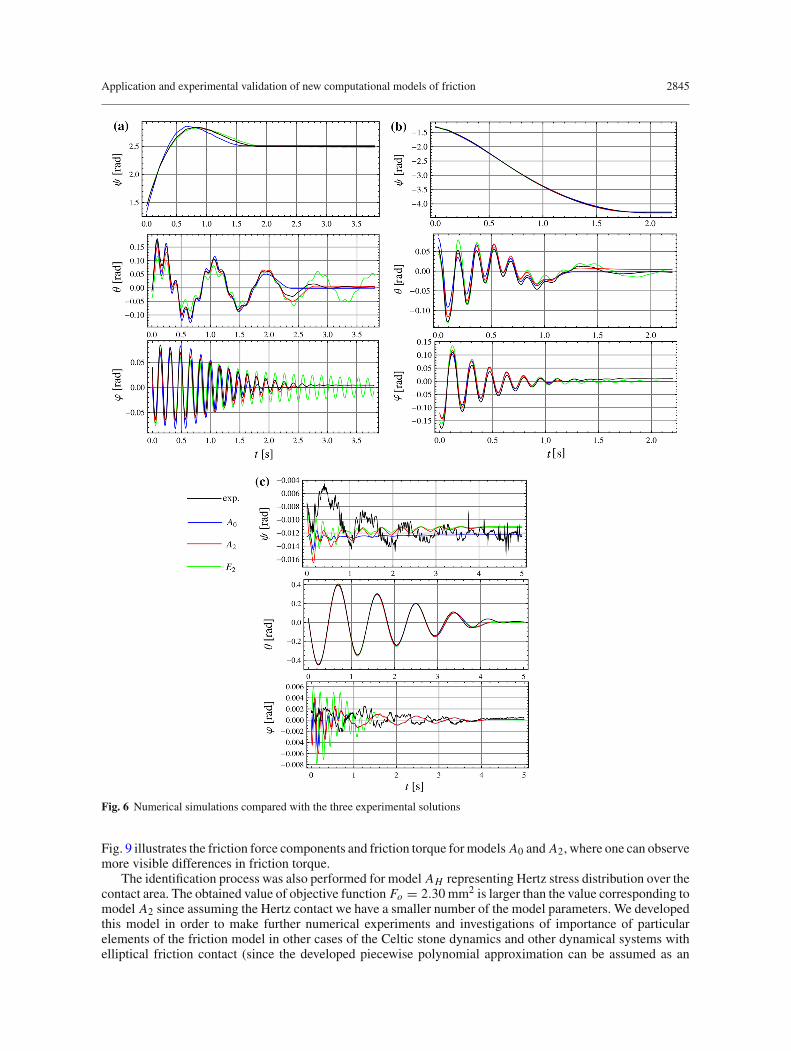
In the experimental investigations we used a rubber plate as a base for the celt. Therefore, we can assumethat the stone was absolutely rigid in comparison with the base plane (the contour resistance for the celt can beneglected). We used three different experimental solutions in the identification processes for different versionsof the contact model. The final fitting of three selected models A0, A2 and E0 to the experimental data ispresented in Fig. 6 exhibiting Euler angles for three different solutions, respectively.

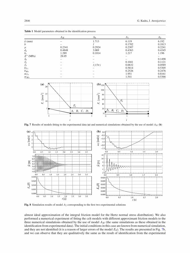
Table 1 exhibits parameters of the selected models (the parameters used in the regularisation process areεT = 10−2.5 and εR = 10−1). The parameters with the values typed in italics are not independent in a givenmodel (they are assumed arbitrarily and do not participate in the identification process). Figure 7a showscorresponding final values of the objective function obtained in the minimisation process for the experimentaldata. One can note that models A1, A2, B1, B2, C1, C2, D1 and D2 cover the dynamics of the celt dynamicsalmost in the same degree (the smallest value of the objective was obtained for model A2: FO = 1.70 mm2),while other ones lead to significantly worse results. It means that such properties like orthotropy of the rollingresistance as well as coupling between friction force and torque play an essential role in the modelling processof the Celtic stone, while other elements are less important.

Figure 8 presents other quantities obtained from the simulation of model A2 (component ω3 of the angularvelocity, normal reaction of base N and total mechanical energy Em), for the two first solutions only. Finally,


Fig. 6 Numerical simulations compared with the three experimental solutions

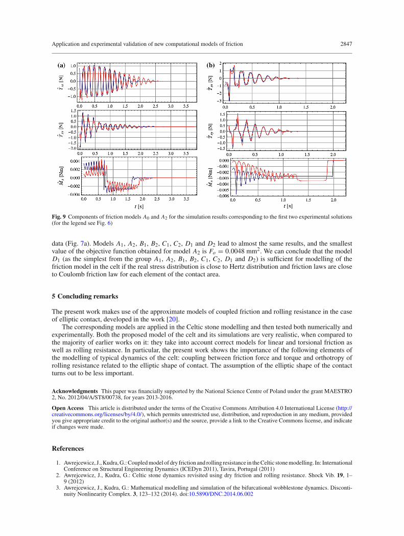
Fig. 9 illustrates the friction force components and friction torque formodels A0 and A2, where one can observemore visible differences in friction torque.

The identification process was also performed for model AH representing Hertz stress distribution over thecontact area. The obtained value of objective function Fo = 2.30 mm2 is larger than the value corresponding tomodel A2 since assuming the Hertz contact we have a smaller number of the model parameters. We developedthis model in order to make further numerical experiments and investigations of importance of particularelements of the friction model in other cases of the Celtic stone dynamics and other dynamical systems withelliptical friction contact (since the developed piecewise polynomial approximation can be assumed as an


Table 1 Model parameters obtained in the identification process

AH A0 A1 A2

a (mm) – 1.713 6.119 6.192b – 1 0.1702 0.1813μ 0.2341 0.2924 0.2307 0.2241da 0.4848 3.069 0.4363 0.4345br 1.289 0.1014 1.217 1.196E∗ (MPa) 28.05 – – –I0 – – – 0.1498I2 – – 0.1041 0.1121I3 – 1/(5π) 0.0632 0.0589bT s – – 0.5814 0.5305bMs – – 0.2526 0.2476mTs – – 1.951 0.8161mMs – – 1.541 0.5366

Fig. 7 Results of models fitting to the experimental data (a) and numerical simulations obtained by the use of model AH (b)

Fig. 8 Simulation results of model A2 corresponding to the first two experimental solutions

almost ideal approximation of the integral friction model for the Hertz normal stress distribution). We alsoperformed a numerical experiment of fitting the celt models with different approximant friction models to thethree numerical simulations obtained by the use of model AH (the same simulations as these obtained in theidentification from experimental data). The initial conditions in this case are known from numerical simulation,and they are not identified (it is a reason of larger errors of the model E0). The results are presented in Fig. 7b,and we can observe that they are qualitatively the same as the result of identification from the experimental


Fig. 9 Components of friction models A0 and A2 for the simulation results corresponding to the first two experimental solutions(for the legend see Fig. 6)

data (Fig. 7a). Models A1, A2, B1, B2, C1, C2, D1 and D2 lead to almost the same results, and the smallestvalue of the objective function obtained for model A2 is Fo = 0.0048 mm2. We can conclude that the modelD1 (as the simplest from the group A1, A2, B1, B2, C1, C2, D1 and D2) is sufficient for modelling of thefriction model in the celt if the real stress distribution is close to Hertz distribution and friction laws are closeto Coulomb friction law for each element of the contact area.

5 Concluding remarks

The present work makes use of the approximate models of coupled friction and rolling resistance in the caseof elliptic contact, developed in the work [20].

The corresponding models are applied in the Celtic stone modelling and then tested both numerically andexperimentally. Both the proposed model of the celt and its simulations are very realistic, when compared tothe majority of earlier works on it: they take into account correct models for linear and torsional friction aswell as rolling resistance. In particular, the present work shows the importance of the following elements ofthe modelling of typical dynamics of the celt: coupling between friction force and torque and orthotropy ofrolling resistance related to the elliptic shape of contact. The assumption of the elliptic shape of the contactturns out to be less important.

Acknowledgments This paper was financially supported by the National Science Centre of Poland under the grant MAESTRO2, No. 2012/04/A/ST8/00738, for years 2013-2016.

Open Access This article is distributed under the terms of the Creative Commons Attribution 4.0 International License (http://creativecommons.org/licenses/by/4.0/), which permits unrestricted use, distribution, and reproduction in any medium, providedyou give appropriate credit to the original author(s) and the source, provide a link to the Creative Commons license, and indicateif changes were made.

References

1. Awrejcewicz, J.,Kudra,G.:Coupledmodel of dry friction and rolling resistance in theCeltic stonemodelling. In: InternationalConference on Structural Engineering Dynamics (ICEDyn 2011), Tavira, Portugal (2011)

2. Awrejcewicz, J., Kudra, G.: Celtic stone dynamics revisited using dry friction and rolling resistance. Shock Vib. 19, 1–9 (2012)

3. Awrejcewicz, J., Kudra, G.: Mathematical modelling and simulation of the bifurcational wobblestone dynamics. Disconti-nuity Nonlinearity Complex. 3, 123–132 (2014). doi:10.5890/DNC.2014.06.002

http://creativecommons.org/licenses/by/4.0/

http://creativecommons.org/licenses/by/4.0/

http://dx.doi.org/10.5890/DNC.2014.06.002


4. Bondi, S.H.: The rigid body dynamics of unidirectional spin. Proc. R. Soc. Lond. A Math. 405, 265–279 (1986)5. Borisov, A.V., Kilin, A.A., Mamaev, I.S.: New effects in dynamics of rattlebacks. Dokl. Phys. 51, 272–275 (2006)6. Caughey, T.K.: A mathematical model of the “Rattleback”. Int. J. Nonlinear Mech. 15, 293–302 (1980)7. Contensou, P.: Couplage entre frottement de glissement et de pivotement dans la téorie de la toupe. Kreiselprobleme

Gyrodynamics, In: IUTAM Symp, Calerina, pp. 201–216 (1962)8. Garcia,A.,Hubbard,M.: Spin reversal of the rattleback: theory and experiment. P.R. Soc. Lond.AMath.418, 165–197 (1988)9. Goyal, S., Ruina, A., Papadopoulos, J.: Planar sliding with dry friction. Part 1. Limit surface and moment func-

tion. Wear 143, 307–330 (1991)10. Gray, A.: Modern Differential Geometry of Curves and Surfaces with Mathematica. pp. 457–480. CRC Press, Boca

Raton (1997)11. Howe, R.D., Cutkosky, M.R.: Practical force-motion models for sliding manipulation. Int. J. Robot. Res. 15, 557–572

(1996)12. Johnson, K.L.: Contact Mechanics. Cambridge University Press, Cambridge (1985)13. Kane, T.R., Levinson, D.A.: Realistic mathematical modeling of the rattleback. Int. J. Nonlinear Mech. 17, 175–186 (1982)14. Kireenkov, A.A.: Combined model of sliding and rolling friction in dynamics of bodies on a rough plane. Mech.

Solids 43, 412–425 (2008)15. Kosenko, I., Aleksandrov, E.: Implementation of the Contensou–Erisman model of friction in frame of the Hertz contact

problem on Modelica. In: 7th Modelica Conference, Como, Italy, pp. 288–298 (2009)16. Kudra, G., Awrejcewicz, J.: Mathematical modelling and numerical simulations of the celtic stone. In: 10th Conference on

Dynamical Systems-Theory and Applications, Lodz, Poland, pp. 919–928 (2009)17. Kudra, G., Awrejcewicz, J.: A wobblestone modelling with coupled model of sliding friction and rolling resistance. In:

XXIV Symposium ”Vibrations in Physical Systems”, Poznan-Bedlewo, Poland, pp. 245–250 (2010)18. Kudra, G., Awrejcewicz, J.: Tangens hyperbolicus approximations of the spatial model of friction coupled with rolling

resistance. Int. J. Bifurc. Chaos 21, 2905–2917 (2011)19. Kudra, G., Awrejcewicz, J.: Bifurcational dynamics of a two-dimensional stick-slip system. Differ. Equ. Dyn. Syst. 20, 301–

322 (2012)20. Kudra, G., Awrejcewicz, J.: Approximate modelling of resulting dry friction forces and rolling resistance for elliptic contact

shape. Eur. J. Mech. A/Solids 42, 358–375 (2013)21. Leine, R.I., Glocker, Ch.: A set-valued force law for spatial Coulomb–Contensou friction. Eur. J. Mech. A/Solid 22, 193–

216 (2003)22. Leine, R.I., Le Saux, C., Glocker, Ch.: Friction models for the rolling disk. In: 5th EUROMECH Nonlinear Dynamics

Conference (ENOC 2005), Eindhoven, The Netherlands (2005)23. Lindberg, J., Longman, R.W.: On the dynamic behavior of the wobblestone. Acta Mech. 49, 81–94 (1983)24. Magnus, K.: Zur Theorie der keltischen Wackelsteine. Zeitschrift für Angewandte Mathematik und Mechanik 5, 54–55

(1974)25. Markeev, A.P.: On the dynamics of a solid on an absolutely rough plane. Regul. Chaotic Dyn. 7, 153–160 (2002)26. Milne-Thompson, L.M.: Elliptic integrals. In: Abramowitz M., Stegun, I.A. (eds.) Hand-Book of Mathematical Functions:

With Formulas, Graphs, and Mathematical Tables, Dover Publications Inc., New York (1972)27. Möller, M., Leine, R.I., Glocker, Ch.: An efficient approximation of orthotropic set-valued laws of normal cone type. In: 7th

EUROMECH Solid Mechanics Conference, Lisbon, Portugal (2009)28. Walker, G.T.: On a dynamical top. Q. J. Pure Appl. Math. 28, 175–184 (1896)29. Wood, S.N.: Minimising model fitting objectives that contain spurious local minima by bootstrap restarting. Biomet-

rics 57, 240–244 (2001)30. Zhuravlev, V.P.: The model of dry friction in the problem of the rolling of rigid bodies. J. Appl. Math. Mech. 62, 705–710

(1998)31. Zhuravlev, V.P.: Friction laws in the case of combination of slip and spin. Mech. Solids. 38, 52–58 (2003)32. Zhuravlev, V.P., Klimov, D.M.: Global motion of the celt. Mech. Solids 43, 320–327 (2008)

Documents

ORIGINAL PAPER Jan Awrejcewicz Application and