Original paper Automated mineralogy and petrology ... · The collection of representative modal mineralogy data as well as textural and chemical information on statistically ... mineralogy,

www.jgeosci.org

Journal of Geosciences, 63 (2018), 47–63 DOI: 10.3190/jgeosci.250

Original paper

Automated mineralogy and petrology – applications of TESCAN Integrated Mineral Analyzer (TIMA)

Tomáš HrsTka1*, Paul GOTTlIeb2, roman skála1, karel breITer1, David MOTl3

1 Institute of Geology, The Czech Academy of Sciences, v.v.i., Rozvojová 269, 165 00 Prague 6-Lysolaje, Czech Republic; [email protected] TESCAN ORSAY HOLDING, a.s., Libušina třída 21, 623 00 Brno, Czech Republic3 TESCAN Brno, s.r.o., Libušina třída 1, 623 00 Brno, Czech Republic* Corresponding author

The collection of representative modal mineralogy data as well as textural and chemical information on statistically significant samples is becoming essential in many areas of Earth and material sciences. Automated Scanning Electron Microscopy (ASEM) systems provide an ideal solution for such tasks. This paper presents the methods and techniques used in the recently developed TESCAN Integrated Mineral Analyzer (TIMA-X) with Version 1.5 TIMA software. The benefits from the use of a fully integrated quantitative energy-dispersive X-ray spectrometry (EDS) and an advanced statistical approach to ASEM systems are demonstrated. Typically, the system can handle more than 500,000 X-ray events per second. Using a common spectral total of 1000 events this represents the acquisition of 500 spectra per second. A number of measurement modes is available to make the most effective use of these spectra depending on the application.For a back-scattered electrons (BSE) map combined with EDS data with spatial resolution of 10 µm, this represents the high-resolution measurement of c. 1 cm2 of a thin section or a polished rock surface in 30 minutes. A patented X-ray spectrum clustering algorithm that lowers the chemical detection limit is described and an example of its use is shown. The modal and textural (liberation, association, size etc.) data produced are statistically robust and provide information across a broad range of Earth and material sciences. A comparison with some other available instruments is also provided together with a number of case studies.

Keywords: TIMA, Automated SEM/EDS, applied mineralogy, modal analysis, artificial intelligence, neural networksReceived: 9 October 2017; accepted: 6 March 2018; handling editor: F. LaufekThe online version of this article (doi: 10.3190/jgeosci.250) contains supplementary electronic material.

instruments are still rather rare and have a limited use because of the difficulties involved in automatically identifying minerals by their color and other properties in reflected light and polarized transmitted light (Pirard 2004; Donskoi et al. 2007; Lane et al. 2008; Poliakov and Donskoi 2014; Berrezueta et al. 2016).

Automated Mineralogy instruments such as QEM-SCAN (Gottlieb et al. 2000) and MLA (Fandrich et al. 2007) were initially designed mainly for use in mineral processing to determine particle mineral liberation from representative samples of plant products (i.e. feeds, con-centrates and tailings). These systems are indeed useful for plant optimization and feed ore characterization for predicting concentrator and leaching performance from ore properties such as grade, elemental deportment, lock-ing, grind size, hardness, and reagent consumption.

Lately, the AM systems have also progressively found their way into many geological research laboratories where they are now being widely used for gathering mineralogical and petrological data. They have been em-ployed to visualize and quantify petrological properties such as alteration, contact zones, fractures, exsolution structures, deformation re-crystallization and mapping

1. Introduction

Information on the modal composition of samples (i.e. volume % or weight % of minerals/phases present) and understanding of their textural relationships are essen-tial in petrologic and petrogenetic studied (Le Bas and Streckeisen 1991; Le Maitre 2002), modelling of ore formation (Rollinson et al. 2011; Smythe et al. 2013; Nie and Peng 2014; Santoro et al. 2014) and in fact in any research related to Earth or material sciences (Gottlieb 2008; Pirrie and Rollinson 2011). Optical microscopy, powder X-ray diffraction (PXRD), scanning electron microscopy (SEM), often supplemented with energy-dispersive X-ray spectroscopy (EDS) and electron-probe microanalysis (EPMA) have represented the key meth-ods used to characterize material properties in the past. Although these techniques still play a crucial role in mineralogy, petrology and geology, the last two decades have seen the widespread use of SEM-based Automated Mineralogy (AM) systems to help identifying minerals by their composition and to quantify their proportions, size and textural relations (Hoal et al. 2009; Pérez-Barnuevo et al. 2013). By contrast, automated optical microscopy

http://dx.doi.org/10.3190/jgeosci.250

Tomáš Hrstka, Paul Gottlieb, Roman Skála, Karel Breiter, David Motl

48

distribution of inclusions as well as other data (Andersen et al. 2009; Haberlah et al. 2010; Knappett et al. 2011; Rollinson et al. 2011; Santoro et al. 2015; Ackerman et al. 2017; Ward et al. 2018).

The AM systems have a number of time- and statistics-optimized analysis methods and modes of operation spe-cifically customized for various industrial and research tasks. These include particle scans, field scans, line scans, specific mineral search routines and other more complex modes (Gottlieb et al. 2000; Fandrich et al. 2007). All these AM systems are based on acquisition, presentation and analysis of hyperspectral data (usually created by a combination of BSE and elemental maps) representing a 2-dimensional (2D) image of flat mineral/phase sec-tions typically for large, statistically significant areas of the sample. A recent trend is that manufacturers of more classic SEM/EDS hardware and elemental quantification software are also starting to follow the example set by AM systems away from traditional (point analysis) and “elemental mapping” to more useful “phase mapping”. Their goal is to create 2D mineral/phase images from geological and other specimens though typically on a smaller scale due to the time constrains (Johnson et al. 2015). It might be foreseen that the two approaches will possibly slowly converge while at the moment combina-tions of both concepts might be necessary to provide the right answers.

In this article we summarize some basic concepts of the use of AM systems in geosciences. Moreover, we demonstrate the latest developments of the TESCAN Integrated Mineral Analyzer (TIMA-X) system and its applications on several typical examples. Some sugges-tions are also made for further developments towards universal, statistically sound instrumental methods for the analysis of minerals and rocks.

2. TESCAN Integrated Mineral Analyzer (TIMA)

2.1. TIMa hardware

The TIMA-X system is based on one to four Energy Dispersive X-ray silicon drift detectors (SDD) attached to standard LM (small) or GM (large) chambers of the TESCAN MIRA (field-emission gun – FEG) or VEGA (thermionic emission – tungsten) platforms.

High throughput is achieved by the use of multiple TIMA EDS detectors operated at very high count rates (in excess of 2,000,000 counts per second, as measured on a platinum standard) and using low-count EDX spectra to identify the minerals at each measurement point (or each homogeneous segment/part of a grain depending on the analysis mode). Hardware and software integration is

also very important. In contrast to classical EDX phase mapping software that requires high count numbers to be collected at each map pixel, the TIMA system is op-timized to deal with rapidly acquired low-count spectra.

The TIMA has specific capabilities for geological applications because of its specialized integration of hardware and software and its high level of automation. The speed, automation and unattended operation allow the researcher to collect detailed data that were not pos-sible to obtain through human-interactive operation of an SEM/EDX system. The multiple EDX detectors, in addi-tion to providing a speed multiplier, have a side-benefit of reducing shading for artefact-free measurement of uneven surfaces with an imperfect polish.

Apart from the back-scattered electron (BSE), second-ary electron (SE), and EDS detectors, the TIMA system can be also accompanied by cathodoluminescence (CL) detector for simultaneous acquisition of CL data during the measurements. An integrated Raman spectroscopy system is also available as an option.

For the larger chamber, up to nine 27 × 47 mm thin sections or fifteen 30 mm diameter or twenty two 25 mm diameter polished blocks can be analyzed in a single batch. The smaller chamber accommodates two 27 × 47 mm thin sections or seven 30 mm diameter or 25 mm diameter polished blocks. A fully automated system (“autoloader”) that is capable of sample exchanges for one hundred 30 mm diameter or 25 mm diameter polished blocks is also available.

All the processing of spectral phase classification is performed already during the data collection in order to use the time efficiently and to produce results by the time when the acquisition is finished. The raw data are also saved together with the processed results to allow for modification of the parameters and off-line reclassifica-tion and/or reinterpretation of the measurements.

2.2. back-scattered electron (bse) image analysis

Imaging and image analysis are fundamental to automated mineral analysis. A stable and well calibrated BSE image is a prerequisite for its proper implementation (Fandrich et al. 2007). The machine calibration is performed on a Fara-day cup and a platinum standard; automated checks and optimizations for long-term measurements are included in the system. At the typical working conditions, the stability of the probe current is better than 0.5 % in 24 hours (for both tungsten and field-emission systems). Consequently, the BSE signal, which depends on the probe current, dis-plays the same (0.5 %) level of stability. It means that if a typical mineral has a mean BSE level of 50.00 arbitrary units, it will not change more than ± 0.25 in 24 hours. The probe current and BSE detector parameters are adjusted


49

automatically to maintain optimum stability. This also al-lows for easy discrimination of phases on a long-term run with BSE image only.

Due to a number of factors the BSE calibration curve of individual BSE detectors is not linear, which creates potential problems in cross-correlation with other sys-tems. Therefore the use of the average atomic number (Z) to monitor the BSE response of a mineral/phase could be suggested to overcome this calibration problem. Lloyd (1987) has examined in detail the use of BSE signal in mineralogy.

It should be noted that the short-term stability and resolution are generally much higher than the long-term one (~0.1 Z compared to ~1 Z or more). This leads to the important ability to use the relative BSE brightness for image/phase segmentation, but gives it a more limited use in the actual mineral/phase identification.

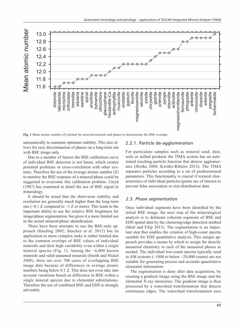
There have been attempts to use the BSE-only ap-proach (Harding 2002; Sánchez et al. 2012) but its application to more complex tasks is rather limited due to the common overlaps of BSE values of individual minerals and their high variability even within a single mineral species (Fig. 1). Among the ~6,000 known minerals and valid unnamed minerals (Smith and Nickel 2008), there are over 700 cases of overlapping BSE image data because of differences in average atomic numbers being below 0.1 Z. This does not even take into account variations based on difference in BSE within a single mineral species due to elemental substitutions. Therefore the use of combined BSE and EDS is strongly advisable.

2.2.1. Particle de-agglomeration

For particulate samples such as mineral sand, dust, soils or milled products the TIMA system has an auto-mated touching-particle function that detects agglomer-ates (Hrstka 2008; Kwitko-Ribeiro 2012). The TIMA separates particles according to a set of predetermined parameters. This functionality is crucial if textural char-acteristics of individual particles/grains are of interest to prevent false association or size-distribution data.

2.3. Phase segmentation

Once individual segments have been identified by the initial BSE image, the next step of the mineralogical analysis is to delineate coherent segments of BSE and EDS spatial data by the clustering/edge detection method (Motl and Filip 2013). The segmentation is an impor-tant step that enables the creation of high-count spectra suitable for EDS quantitative analysis. This unique ap-proach provides a means by which to assign the directly measured chemistry to each of the measured phases as needed. The individual low-count spectra typically used in AM systems (~1000 to below ~20,000 counts) are not suitable for generating precise and accurate quantitative elemental information.

The segmentation is done after data acquisition, by creating a gradient image using the BSE image and the elemental X-ray intensities. The gradient image is then processed by a watershed transformation that detects continuous edges. The watershed transformation uses

dolo

mite

labra

dorite

mic

roclin

eo

rth

ocla

se

tre

mo

lite

adula

ria

sanid

ine

sp

ine

la

no

rth

ite

byto

wnite

clin

ochlo

regla

ucophane

heula

ndite-C

aanth

ophylli

tem

usco

vite

en

sta

tite

gypsum

leu

cite

magnesio

axin

ite

win

chite

zo

isite

ch

ryso

lite

gedrite

pre

hnite

pyro

pe

sta

uro

lite

actin

olit

em

agnesio

horn

ble

nde

ferr

oa

xin

ite

phlo

gopite

ankerite

clin

ozo

isite

dio

psid

eedenite

parg

asite

tsch

erm

akite

11.6

11.8

12.0

12.2

12.4

12.6

12.8

13.0

Me

an

ato

mic

nu

mb

er

Fig. 1 Mean atomic number (Z) plotted for selected minerals and phases to demonstrate the BSE overlaps.


50

Line mapping c)

10 K PARTICLES ~ 22 min (660 000 analytical points)

Point spectroscopyHigh resolution mapping a)

10 K PARTICLES ~ 168 min (5 040 000 analytical points)

b)

10 K PARTICLES ~ 2 min (40 000 analytical points)

Dot mapping d)

10 K PARTICLES ~ 43 min (1 280 000 analytical points)

BSE 2,5 µm & EDS 2,5 µm step

BSE 2,5 µm & EDS 5 µm step + Single EDS for small grainsBSE & EDS 2,5 µm step on a line - lines 30 µm apart

BSE 2,5 µm & Single EDS per segment/grain

20 µm

Quartz Feldspar Topaz Zircon

EDS ANALYTICAL POINT BSE GRID GREATEST INSCRIBED CIRCLE


51

2.4.2. TIMa Point spectrometry (TPs)

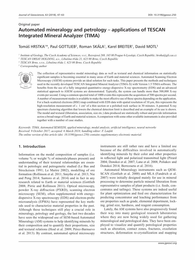
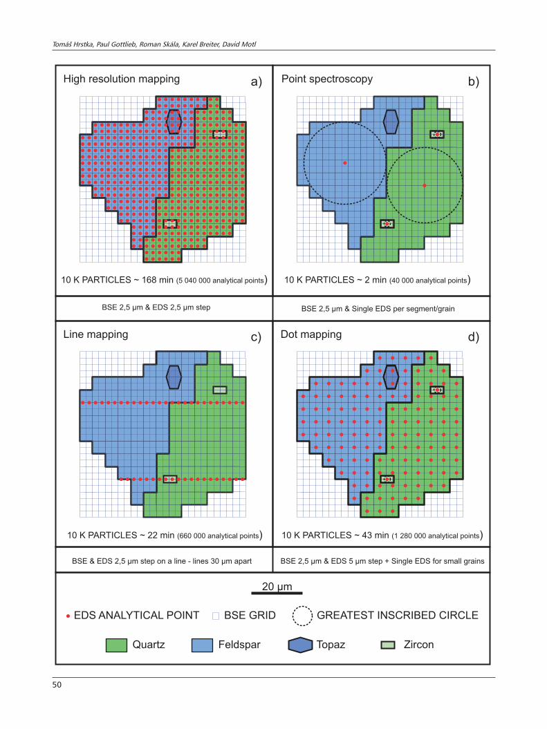
In point spectrometry, individual particles and distinct phases/grains are determined using the BSE image only. Areas of similar BSE brightness are identified as homoge-neous regions. The center of the largest inscribed circle of each region is then used as a single X-ray analysis point to identify a mineral or a phase representing the entire region (Fig. 2b). This method is very fast, but cannot resolve two adjacent phases with similar mean atomic numbers but different chemistry and thus can lead to large areas of misclassification (Fandrich et al. 2007). It can be used to handle various geological samples as far as the minerals of interest have sufficient BSE grey level contrast. This can be difficult to predict for unknown samples and thus only well-known/previously studied samples can be recommended for this type of analysis. Its definite advantage is the high speed as only a single spectrum is collected per homogeneous BSE segment. As stated previously, Z resolution is highly dependent on measurement parameters like beam current, brightness/contrast settings of the instrument, quality of the sample surface, focus etc. (Lloyd 1987; Harding 2002).

2.4.3. TIMa line Mapping (TlM)

Line mapping is used to reduce X-ray acquisition time but still maintain some textural information such as mineral grain size and mineral association. For line map-ping each field is covered by equidistant horizontal lines using a specified “line spacing” (Fig. 2c). The electron beam moves along each line in regularly distributed measurement points using the specified “pixels spacing”. At each point, the BSE level is determined, if the BSE level is above the threshold, the beam is kept on this spot until the specific number of X-ray counts from the spec-trometer is collected. The beam then moves to the next point. When the pre-determined limit of the line length (field size) is reached, the beam moves to the next line and starts over. This procedure is repeated until all lines covering the selected field have been scanned.

Then, the individual lines are divided into multiple linear sections using the combination of the BSE level and the EDS data to determine boundaries between dis-tinct phases.

The EDS data from the measurement points within each line section/segment are summed. The mean BSE level for each line section/segment is determined as well. The mean BSE level and the combined spectrum are used to classify the line sections using the specified classifica-tion scheme to determine the mineral/phase.

The advantage of this method in comparison with Point Spectrometry method is that it resolves boundaries between phases with similar mean atomic number but

one parameter – the minimum gradient that is regarded as an edge. The value of this parameter is controlled by the user. Whenever two segments in contact have a similar composition and, as a result, the gradient between them is low, they are merged into a single segment rather than remain separated. The minimum gradient parameter is used to increase the separation of such phases. If it is too high, the software creates too many segments and, as a result, this yields large datasets and off-line reclassification and data processing takes more time.

2.4. Mineral identification by bse and X-ray analysis (acquisition Modes)

The TIMA currently has four X-ray analysis scanning modes to identify mineral species: High-resolution mapping, Point spectrometry, Line mapping and Dot mapping. These modes have been developed to econo-mize on the X-ray acquisition time. Each mode can be further optimized to perform specific tasks. The most important optimization parameters are the number of X-ray counts per analytical spectrum and the distance spread (pixel spacing) of individual analytical points (Fig. 2).

2.4.1. TIMa High-resolution Mapping (THrM)

In this mode the TIMA first collects the BSE signal at the analytical point and then one X-ray spectrum (typically > 1000 counts) for each point over a regular grid within each segmented particle. The BSE level is used as a threshold so that if the BSE level is outside the specified range (e.g. epoxy), the X-ray spectra are not collected in order to save run time (Fig. 2a). This method can be used to handle various rocks with complex textures or other samples where detailed resolution is required. Due to the optimized data processing and simultaneous use of four SDD detectors, the TIMA acquisition rate, when trans-lated into measurement time elapsed, is approximately 30 minutes for the analysis of 1 cm² of a granitic rock at 10 µm pixel spacing and 1000 counts per spectrum per point (in the THRM mode). This acquisition mode, to-gether with the liberation analysis, can be used to collect modal and textural data (e.g., Žák et al. 2016).

Fig. 2 Sketch illustrating the principles of TIMA acquisition modes. a – High-resolution mapping using the same regular BSE and EDS analysis grid. b – Point mapping uses BSE only to segment the image and collect single EDS spectra from each phase discriminated based on BSE. c – Line mapping records one-dimensional profiles through the sample. d – Dot mapping uses different pixel spacing for the BSE and EDS data collection.


52

different chemistry, and still provides high speed. This method gives only bulk association and modal data due to one dimensional cuts through the particles rather than two dimensional maps of each particle. However, it has the advantage of enabling the measurement of more particles to obtain better sampling statistics.

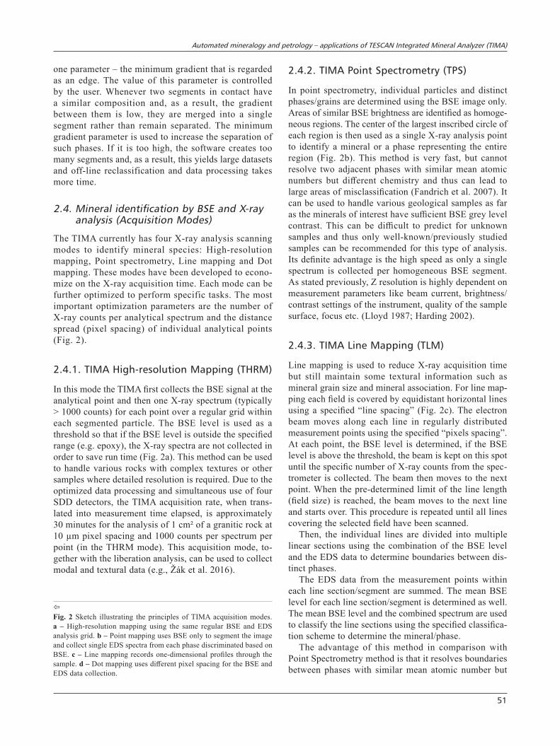
It can be used to handle various complex geological samples with the advantage of high speed if the collection of the full set of quantitative textural data is not critical. It also stores BSE images of each field so the operator can assess the quality of the results (perform QA, i.e. quality assurance) easily and get detailed qualitative information on textures from the BSE images (Fig. 3).

2.4.4. TIMa Dot Mapping (TDM)

Dot mapping imposes a BSE grid with specific resolution (determined as “pixel spacing”) over the entire sample, or specific particles/grains thereof (based on the BSE threshold). It uses the acquired image to segment areas of homogeneous BSE intensities and identifies the center

Fig. 3 Example of thin section modal analysis by the means of TIMA Line Mapping (TLM). Quantitative modal data are obtained fast (10 min for the whole thin section) while textural context is provided by the simultaneously acquired BSE image.

a)

b)c)

d)

e)

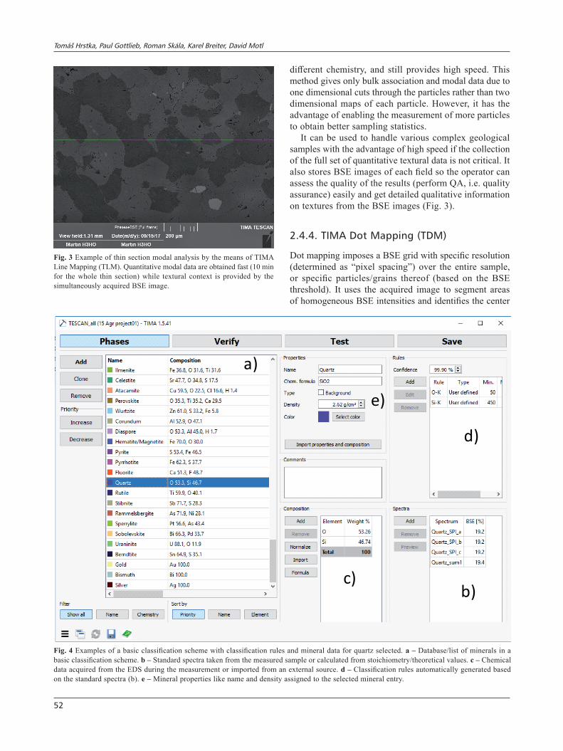
Fig. 4 Examples of a basic classification scheme with classification rules and mineral data for quartz selected. a – Database/list of minerals in a basic classification scheme. b – Standard spectra taken from the measured sample or calculated from stoichiometry/theoretical values. c – Chemical data acquired from the EDS during the measurement or imported from an external source. d – Classification rules automatically generated based on the standard spectra (b). e – Mineral properties like name and density assigned to the selected mineral entry.


53

of greatest inscribed circle. In the second pass it creates a rectangular grid for X-ray acquisition with resolution spec-ified by the “dot spacing” over each of the “preliminary” BSE phase segments determined in the first step. The com-bination of the high-resolution BSE image and the lower-resolution EDS data is used to greatly improve the phase segmentation when the preliminary segments comprise of multiple minerals/phases with similar Z but different chemistry. X-ray data from zones of similar BSE and EDS signals are summed to produce single higher quality spectra for each final segment. Average BSE and summed spectra from each final segment are used to determine the mineral identity. The origin of the second X-ray data grid is centered on each segment. This means that even grains smaller than the “dot spacing” of the X-ray data grid are characterized by at least a single X-ray analysis point.

The Dot Mapping method provides an excellent compromise between the high-resolution mapping and the point spectrometry method in terms of speed versus textural/information detail. As a single X-ray spectrum is collected even for particles smaller than the “dot spac-ing”, even the smallest bright particles and textures are recorded (Fig. 2d).

The data collection procedure can be customized for specific tasks by the variation of its parameters (e.g. very fast analysis of a thin section – Slavík et al. 2016; Acker-man et al. 2017) or very detailed, submicron analysis of complex dust particles or soil contaminants (Harvey et al. 2017; Hrstka et al. 2017a, b).

2.5. Mineral standards library (Classification scheme)

Mineral identification through BSE signals, EDS data or the combination of both requires a library of mineral compositional limits/mineral definition rules or standard spectra (Classification scheme in TIMA – Fig. 4). Any unknown spectra collected from a point or a segment, together with related information from other detectors (BSE, CL, SE etc.), are used to find the closest or first match to the records in the database providing mineral/phase identification. For TIMA, a first match principle is used being based on the combination of mineral definition rules, either determined automatically (from a “standard spectrum” or calculated from a theoretical mineral/phase composition) by the system or created by the user from BSE, X-ray spectral windows counts and/or their ratios. The automation in creating the rules based on standard spectra significantly reduces the time spent on building a classification scheme, especially when tens or hundreds of potential phases are involved. A classification scheme provides not only the name of the identified phase, but also information on its exact chemistry and density needed in all subsequent modal or elemental deportment calcula-

tions. The phase chemistry for a specific classification scheme can be based directly on the collected EDS data, taken from the theoretical stoichiometric composition, or entered manually based on a relevant external analysis [e.g. EMPA, Laser-Ablation Inductively Coupled Plasma Mass Spectrometry (LA-ICP-MS), Proton-Induced X-ray Emission (PIXE), or Micro X-ray fluorescence (µXRF)]. These external analyses can account for elements which are sometimes present in phases in trace amounts but are important for the overall element distribution of the sample (e.g. gold in pyrite, nickel in goethite). This is particularly important for phases containing elements with concentra-tions below EDS detection limits.

The density as a first approximation is based on the mineral/phase identity or external study of the mineral/phase. There is no direct means currently available for measuring mineral density inside a SEM.

Built-in QA routines provide a confusion matrix to point the user to potential problematic phases which could be misidentified/mismatched due to overlaps in the classification parameters. Basic classification schemes are provided with the system as a starter kit. The Webmineral database (Mineralogical database 2017) is included to al-low for quick and easy creation of classification scheme entries from theoretical mineral formulae matching the specific project needs.

In order to further simplify the current workflow, a supervised or fully autonomous system based on artificial intelligence, machine learning and neural networks is under development (Hrstka et al. 2017a).

2.6. Measurement analysis types

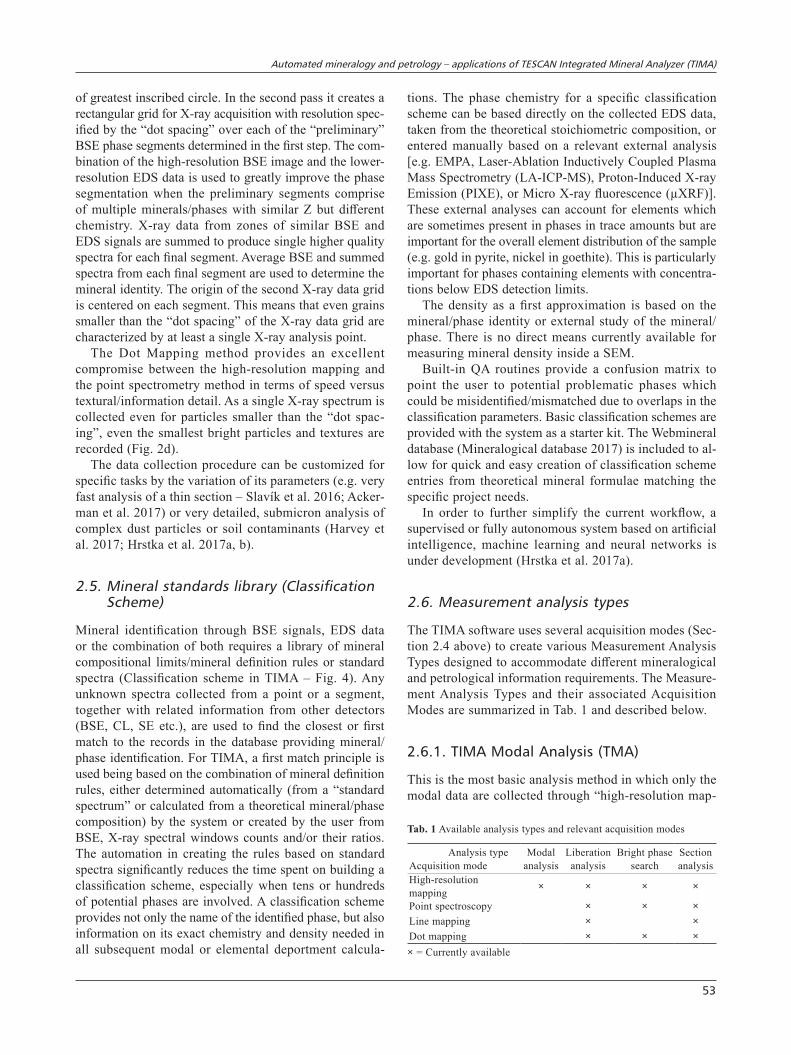
The TIMA software uses several acquisition modes (Sec-tion 2.4 above) to create various Measurement Analysis Types designed to accommodate different mineralogical and petrological information requirements. The Measure-ment Analysis Types and their associated Acquisition Modes are summarized in Tab. 1 and described below.

2.6.1. TIMa Modal analysis (TMa)

This is the most basic analysis method in which only the modal data are collected through “high-resolution map-

Tab. 1 Available analysis types and relevant acquisition modes

Analysis type Acquisition mode

Modal analysis

Liberation analysis

Bright phase search

Section analysis

High-resolution mapping × × × ×

Point spectroscopy × × ×Line mapping × ×Dot mapping × × ×× = Currently available


54

ping” (see Section 2.4.1). It can be applied to particulate material or thin sections and polished blocks to obtain statistically robust modal data. It is in a way similar to classical point counting (Glagolev 1934; Larrea et al. 2014 and references therein), but is able to collect more than 500 analytical points per second!

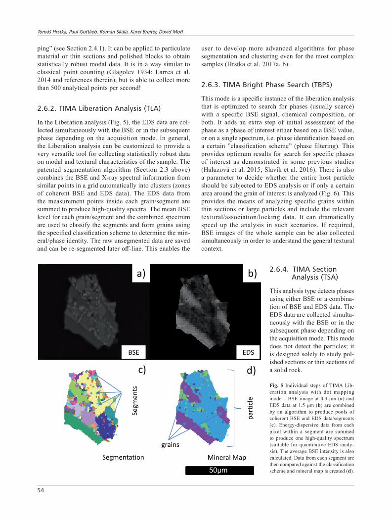
2.6.2. TIMa liberation analysis (Tla)

In the Liberation analysis (Fig. 5), the EDS data are col-lected simultaneously with the BSE or in the subsequent phase depending on the acquisition mode. In general, the Liberation analysis can be customized to provide a very versatile tool for collecting statistically robust data on modal and textural characteristics of the sample. The patented segmentation algorithm (Section 2.3 above) combines the BSE and X-ray spectral information from similar points in a grid automatically into clusters (zones of coherent BSE and EDS data). The EDS data from the measurement points inside each grain/segment are summed to produce high-quality spectra. The mean BSE level for each grain/segment and the combined spectrum are used to classify the segments and form grains using the specified classification scheme to determine the min-eral/phase identity. The raw unsegmented data are saved and can be re-segmented later off-line. This enables the

user to develop more advanced algorithms for phase segmentation and clustering even for the most complex samples (Hrstka et al. 2017a, b).

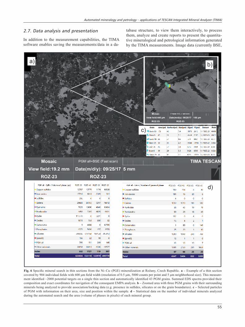
2.6.3. TIMa bright Phase search (TbPs)

This mode is a specific instance of the liberation analysis that is optimized to search for phases (usually scarce) with a specific BSE signal, chemical composition, or both. It adds an extra step of initial assessment of the phase as a phase of interest either based on a BSE value, or on a single spectrum, i.e. phase identification based on a certain ”classification scheme” (phase filtering). This provides optimum results for search for specific phases of interest as demonstrated in some previous studies (Haluzová et al. 2015; Slavík et al. 2016). There is also a parameter to decide whether the entire host particle should be subjected to EDS analysis or if only a certain area around the grain of interest is analyzed (Fig. 6). This provides the means of analyzing specific grains within thin sections or large particles and include the relevant textural/association/locking data. It can dramatically speed up the analysis in such scenarios. If required, BSE images of the whole sample can be also collected simultaneously in order to understand the general textural context.

2.6.4. TIMa section analysis (Tsa)

This analysis type detects phases using either BSE or a combina-tion of BSE and EDS data. The EDS data are collected simulta-neously with the BSE or in the subsequent phase depending on the acquisition mode. This mode does not detect the particles; it is designed solely to study pol-ished sections or thin sections of a solid rock.

pa

rtic

le

grains

Segmentation Mineral Map

50µm

BSE EDS

a) b)

d)c)

Se

gm

en

ts

Fig. 5 Individual steps of TIMA Lib-eration analysis with dot mapping mode – BSE image at 0.3 μm (a) and EDS data at 1.5 μm (b) are combined by an algorithm to produce pools of coherent BSE and EDS data/segments (c). Energy-dispersive data from each pixel within a segment are summed to produce one high-quality spectrum (suitable for quantitative EDS analy-sis). The average BSE intensity is also calculated. Data from each segment are then compared against the classification scheme and mineral map is created (d).


55

2.7. Data analysis and presentation

In addition to the measurement capabilities, the TIMA software enables saving the measurements/data in a da-

tabase structure, to view them interactively, to process them, analyze and create reports to present the quantita-tive mineralogical and petrological information generated by the TIMA measurements. Image data (currently BSE,

a)b)

c)

d)

Fig. 6 Specific mineral search in thin sections from the Ni–Cu–(PGE) mineralization at Rožany, Czech Republic. a – Example of a thin section covered by 904 individual fields with 600 μm field width (resolution of 0.5 μm, 5000 counts per point and 5 μm neighborhood size). This measure-ment identified ~2000 potential targets on a single thin section and automatically identified 43 PGM grains. Summed EDS spectra provided their composition and exact coordinates for navigation of the consequent EMPA analysis. b – Zoomed area with three PGM grains with their surrounding minerals being analyzed to provide association/locking data (e.g. presence in sulfides, silicates or on the grain boundaries). c – Selected particles of PGM with information on their area, size and position within the sample. d – Statistical data on the number of individual minerals analyzed during the automated search and the area (volume of phases in pixels) of each mineral group.


56

2.8. User-defined expressions and queries

User-defined expressions are used for particle classifica-tion, filtering and sorting. This provides the best opportu-nity to explore the data for any specific research project and create outputs based on categorizers. Examples could be plotting drilling log data from several samples studied during a drilling campaign, geological mapping, provenance study, creating complex tables for dashboards and interactive real-time work with data.

2.8.1. expressions and queries

The TIMA software has the ability to select multiple sub-sets of measured data from the database by user-defined queries. The syntax is somewhat similar to a Structured Query Language (SQL) approach but is specifically tai-lored to AM requirements.

Queries can be used to extend capabilities of the exist-ing predefined reports or to create new specific custom reports. The query can be understood as a function that derives a statistics from a (sub-) population of objects, for example total mass of a phase. Depending on the report type, the statistic assessment is applied to all selected measurements or a subpopulation thereof classified using the categorizer or created by filtering of a certain type of objects. This is a highly customizable way to explore the data and to provide appropriate interpretation suitable for every specific mineralogy/petrology research or industry driven task. A suitable example could be looking at the deportment/distribution of a certain element among dif-ferent mineral phases or even individual lithotypes pres-ent in the sample.

2.8.2. Filtering

Filters are used to create an object (e.g. particle or min-eral grain) sub-set for subsequent inclusion in the com-putation and display of images, tables and charts. A filter can be as simple as manually including or excluding a sub-set of measurements or it can be more complex, based on user-defined criteria.

Multiple object properties can be combined in a filter through expressions or through a selection of multiple filters from a pre-defined table. Multiple filters are a form of the logical AND operator; an object must pass all the conditions in a filter group (referred to as “expression”) to be included.

An example of application is the location of grains of zircons in a heavy minerals grain mount for later analysis by e.g. EPMA or LA-ICP-MS. A multiple filter can eas-ily be defined to show particles with zircon grains larger than 30 µm (e.g. combined size (size>30) and phase (MineralPercent(Zircon)>90). It can also be

SE and CL) are combined with the elemental composition and densities of the identified phases/minerals on a pixel by pixel (or segment by segment) basis to produce a va-riety of mineralogical data. There are several predefined reports/data analysis tools that are available; the informa-tion they provide is nearly self-explanatory:● Panorama, Fields, Particle viewer, and Grain view

are used to visualize the images of grains, particles, individual analyzed fields or whole samples.

● Mineral association, Mineral liberation, Mineral locking, Mineral release, Grain size Phase SSA, Porosity and Particle constituents are designed to provide values related to textural analysis of the samples. For the examples of textural analysis reader is referred to e.g. Lastra (2007) or Pérez--Barnuevo et al. (2013).

● Elemental Mass, Elemental deportment and Mineral Mass provide results on modal distribution of mine-rals/phases and the distribution of elements between individual phases/minerals. The performance of a theoretical perfect concentrator is given by the Gra-de-Recovery report. It is used to compare with the actual performance of a mineral concentrator plant and asses its efficiency. See Lotter et al. (2011) and Altree-Williams et al. (2015) for more details on the use of grade-recovery data.An important type of report is the Assay reconcilia-

tion that provides a QA check against an independent chemical assay of a sample. If a representative sample is selected, then two aliquots can be made. The first is measured by TIMA and the modal mineralogy is combined with the mineral chemistries and densities to calculate a theoretical elemental assay of the sample. The calculated assay is compared to the XRF, ICP-MS or any other independent bulk chemical analysis of the other representative aliquot. Very good reconciliation can be achieved but some potential pitfalls related mainly to the sampling statistics and the quality of the preparation of the samples were identified and discussed in literature (Hrstka 2008, 2012; Johnson et al. 2015; Lastra and Paktunc 2016; Pooler and Dold 2017).

Measurement properties report tabulates measure-ment parameters such as the measurement type, acqui-sition mode, pixel spacing with operational statistical values such as measurement time, area, number of fields, number of particles and number of analytical points acquired.

There are also general-purpose reports, which include the Generic output, Particle category and Category view-er. Each of them can be customized for a particular pur-pose by using mineral particle and elemental properties from the measured data in expressions and queries. These reports represent the full potential of the AM systems.


57

used to exclude some artefacts from the measurements based on their size, composition and/or shape. Filtering is also very useful for interactive work where it can be used to focus onto a small subset of relevant information (e.g., particles with density > 3 g/cm3 and size > 100 µm).

2.8.3. sorting

Sorting allows the user to arrange objects (e.g. particles or grains) based on their properties. It allows the user to visualize particles based on their size, mineral or element contents, density or other parameters. This is particularly useful while performing the quality control on the results or for understanding data present in calculations visually. An example would be to sort all the zircon grains found in a thin section by their size or sort all the grains found based on their density to evaluate the phases likely allowing the LA-ICP-MS dating. Another example would be to sort all the particles/grains by element mass, or phase mass to see the most important carriers of a certain element/phase in the tested sample (e.g. to evaluate the possible nugget effect of one big grain hosting most of a certain element).

2.8.4. Categorizing

Unlike the filters that are used to exclude particles/data from charts, tables and visualization the categorizers are employed to subdivide the data into user-defined categories (classes). Each category is defined by a set of rules, based on properties of the data objects (e.g. par-ticle size, liberation, phase contents, elemental content etc.). Combinations of rules of different kind are also possible. Categories are now used only in specific report types. A simple example would be to create individual sub-groups of particles based on their textural properties like liberation or association. (e.g., Area % (Min-eral)>=80 <=100, Area % (Mineral)>=60 <=80, Area %(Mineral)>=20 <=60, Area % (Mineral)>0 <=20). For particulate samples this would create classes of nearly free (liberated) mineral of interest, relatively liberated mineral of interest, mixed particles composed of mineral of interest and other phases and particles with low proportion of the mineral of interest. While liberation or association information are mostly used in mineral processing to model the theoreti-cal behavior of particles in a physical separation unit like cyclone or flotation cell (Sandmann and Gutzmer 2013; Jordens et al. 2016) the same concept can be easily ex-tended to classifying the rock fragments or thin sections according to their petrological classification (“lithotyp-ing”) (Haberlah et al. 2010; Knappett et al. 2011; Higgs et al. 2015). Automated classification according to the QAPF classification scheme for igneous rocks (Le Maitre 2002) can be an excellent example. As we can use the

combined modal and textural criteria at the same time for categorizing, this approach of automated rock type classification can be also adopted for sedimentary and, to a certain degree, even to metamorphic rocks.

2.8.5. Mineral grouping

As the list of phases/minerals identified in a sample can be quite extensive, a grouping function allows a mineral group to be defined and further treated as individual mineral phase (e.g. all feldspars, all amphiboles, all sili-cates, all heavy minerals etc.). Minor minerals of little importance to an analysis could be automatically grouped as “other” based on a minimal mass in the sample thresh-old. Several groupings with different level of detail for classification of minerals/phases (e.g. species, series, subgroups, groups) can be used at the same time to simplify the navigation through data or results reporting (e.g. detailed grouping for modal analysis and simplified grouping for textural/petrographic analysis).

3. Case studies

The many measurement types and acquisition modes of the TIMA system were tested at the Institute of Geology of the Czech Academy of Sciences in numerous scientific projects in areas spanning from ore geology (Haluzová et al. 2015), through paleontology and paleoecology (Slavík et al. 2016), petrology (Svojtka et al. 2016; Žák et al. 2016; Ackerman et al. 2017; Breiter et al. 2017, 2018), archaeology (Neumannová et al. 2016), ecol-ogy/contaminated soil analysis (Harvey et al. 2017) to dust analysis (Hrstka et al. 2017b). The majority of the applications have been linked to the fast collection of statistically robust data on mineral composition and tex-tural characteristics, together with the ability to quickly search for specific minerals or phases within geological samples. To illustrate the novel approach of Dot map (TDM) analysis and Bright phase search (TBPS) in thin sections (specific mineral search), selected case studies on applications of the TIMA AM technology are briefly outlined in this section.

3.1. Case study 1 – fast automated search for specific minerals in thin and polished sections

The modal analysis in combination with Bright phase search (TBPS) was used to provide better constraints on the nature, conditions of formation and evolution of sulphide mineralization at Rožany deposit, northernmost Bohemian Massif (Haluzová et al. 2015). Studied sam-ples were collected in two abandoned quarries (the first


58

quarry: N 51°2.09'; E 14°27.08', the second: N 51°2.05'; E 14°27.87') in 2014–2015. In total, six samples of mas-sive ores, two of disseminated ores and one of the barren dolerite were selected from a large sample collection. These were used to investigate the mineralogy and char-acteristics of the Ni–Cu–(PGE) mineralization.

The distribution of the individual platinum-group minerals (PGM) was established through the detailed “TBPS” analysis. For the eight studied samples, over 29,000 potential target grains (0.5–200 µm in size) were identified based on the BSE brightness. By matching the EDS signature to the classification scheme, 63 PGM grains were located in less than 10 h. Their identifica-tion through the automated system was crosschecked by a detailed manual SEM/EMPA investigation of selected individual grains located through the TIMA analysis. The correlative TIMA workflow allowed exporting the co-ordinates of target grains into the EPMA system. In addition to the previous studies, minerals moncheite [(Pt,Pd)(TeBi)2] and michenerite [(Pd,Pt)BiTe] were revealed and a possible unnamed Pt–As–Te phase was also noted. During the TIMA investigation the PGM were found not only directly in the base-metal sulphides or at sulphide–silicate grain boundaries, but also in matrix silicates, amphiboles and/or chlorites. This indicates that at least part of the PGM was related to the late-stage hydrothermal processes.

The distribution of the individual PGE was shown to correlate with the likely incorporation of Iridium group of PGM (I-PGM) in Ni-bearing sulphides in the form of solid solution. The results are in agreement with the findings of Sandmann and Gutzmer (2015) indicating that high number of polished sections needs to be studied to provide statistically valid data on PGM distribution. The automated approach enabled fast localization and identification of PGM among the BSE-bright phases within the samples. It also helped to assess the economic potential of the deposit and to constrain the ore genesis in comparison with other Ni–Cu–(PGE) mineralizations (Haluzová et al. 2015).

3.2. Case study 2 – palaeoecological characterization of the lochkovian–Pragian boundary

A highly automated approach was used in the paleoeco-logical characterization of the sedimentary record across the Lochkovian–Pragian boundary in the Spanish Central Pyrenees to explain the origin of the anomalously high (17 to 26 ppm) Th contents in this stratigraphic interval as well as to better understand the potential source areas and provenance of impurities in the carbonates (Slavík et al. 2016). In this case the use of AM allowed us to trace the source of Th and identify monazite as its main carrier.

Also the spatial distribution of magnetite in the samples was used to shed some light on the magnetostratigraphic properties of the rocks.

The TIMA has found over a thousand monazite grains, 1–80 µm across, some displayed a complex inner structure formed by visible relict nuclei crystals or crystoclasts rich in Th, surrounded by altered overgrowths with a spongy or crystalline appearance considerably depleted in Th. The outermost rims were again enriched in Th. From the detailed analysis of individual monazite grains, the identi-fied textures and comparison to similar material from other locations worldwide, understanding on the paleoclimate and its evolution was improved (Slavík et al. 2016 and refer-ences therein). Based on this published example, automated mineralogy data together with systematic specific mineral search and related deportment of elements of interest in thin sections and rock samples offers wide and promising applications in identification of source areas, paleoclimate reconstructions and provenience studies in general.

3.3. Case study 3 – Cínovec/Zinnwald Pluton, krušné Hory Mts./erzgebirge

The 1597 m deep borehole CS-1 located in the center of the Cínovec Pluton represents an ideal object for evalua-tion of vertical structure of rare-metal bearing magmatic systems (Štemprok and Šulcek 1969; Štemprok 2016; Breiter et al. 2017).

A combination of textural and chemical methods was applied to the whole-rock and mineral samples to define chemical and mineral composition of all granite facies and to assess the relative role of magmatic and metasomatic processes during differentiation of the pluton and forma-tion of the Cínovec/Zinnwald Li–Sn greisen deposit.

One of the tasks was the estimation of temperature of crystallization of the main granite facies using feldspar geothermometer (Whitney and Stormer 1977).

The Cínovec Pluton is composed of two principal units: a suite of albite–zinnwaldite granites forms upper part to the depth of 735 m, whereas the suite of biotite granites follows in interval 735–1597 m. Both suites locally comprise fine-grained distinctly porphyritic fa-cies (traditionally termed as microgranites) with perthite phenocrysts 5–10 mm in size.

To calculate the primary perthite composition and es-timate the temperature of its crystallization, typical sam-ples of both microgranites (zinnwalditic from the depth of 413 m and biotitic from the depth of 880 m) were selected. The surface of thin section was divided into a square grid (c. 300 squares per a standard section) and the abundances of Ab and Kfs in each square were measured using TIMA. The results of the squares composed only of perthite were highlighted, and carefully inspected to verify if all of the albite really represented perthite ad-


59

mixtures. After the exclusion of all squares containing also the likely primary albite, the mean composition of perthite within the section was calculated. The primary composition of the alkali feldspars was obtained on the basis of modal abundances of the K- and Na-phases and their chemical compositions measured by the EMPA. The calculated Ab component in primary feldspar decreases from c. 40 % in the biotite microgranite (BtGm) at the depth of 860 m to c. 21 % in the zinnwaldite microgranite (ZiGm) at the depth of 413 m. Considering the decrease in pressure during magma ascent in the Eastern Erzge-birge (6 → 1 kbar; Müller et al. 2005) and the primary composition of associated plagioclase (An15 in the BtGm and An05 in the ZiGm), the temperature of the perthite equilibration decreases upwards from approximately 800 °C to 550 °C. In this case the automated collection of modal and textural data allowed better understanding of the granite evolution as detailed in Breiter et al. (2017).

3.4. Case study 4 – estimation of mineral and chemical composition of layered aplite–pegmatite dykes: “line rocks” of Megiliggar, Cornwall

Genetic relation between granitic pegmatites and gran-ites, i.e. a search for the source of particular pegmatite

body in some neighboring granite pluton, is the topic of a long-term debate (London 2008). Despite intense search, localities enabling to study the direct transition from granite pluton to rare-element pegmatite dykes are scarce. One of the best examples is the Megiliggar Rock at the SE contact of the Tregonning Granite in Cornwall, SW England (Stone 1969). Spectacular outcrops in the coastal cliff show the transition from the granite pluton through dyke leucogranites to aplites and pegmatites. The TIMA was used for a detailed study of the modal and chemical compositions of layered parts of the dykes, where the thickness of individual layers varies between 1 and 5 mm (Breiter et al. 2018).

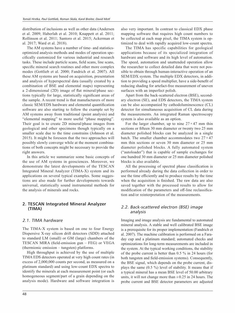
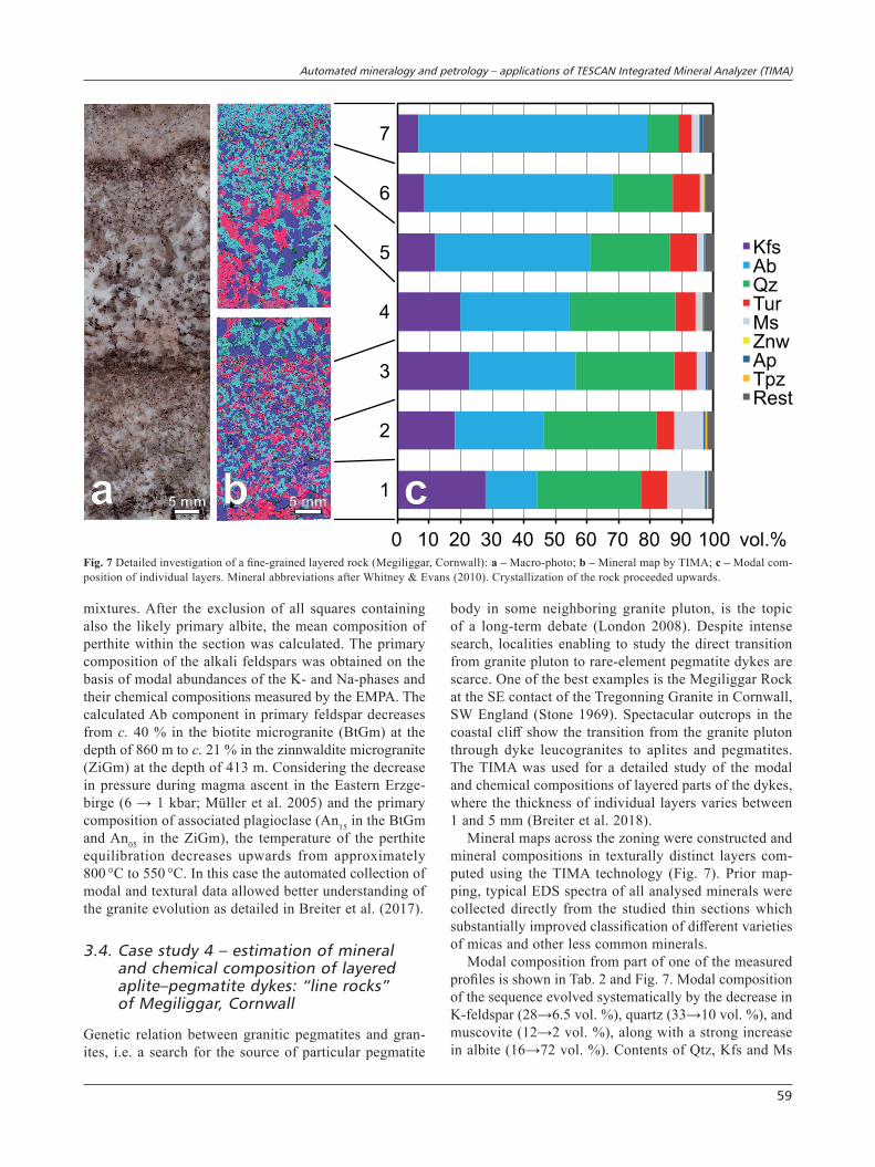
Mineral maps across the zoning were constructed and mineral compositions in texturally distinct layers com-puted using the TIMA technology (Fig. 7). Prior map-ping, typical EDS spectra of all analysed minerals were collected directly from the studied thin sections which substantially improved classification of different varieties of micas and other less common minerals.

Modal composition from part of one of the measured profiles is shown in Tab. 2 and Fig. 7. Modal composition of the sequence evolved systematically by the decrease in K-feldspar (28→6.5 vol. %), quartz (33→10 vol. %), and muscovite (12→2 vol. %), along with a strong increase in albite (16→72 vol. %). Contents of Qtz, Kfs and Ms

0 10 20 30 40 50 60 70 80 90 100

1

2

3

4

5

6

7

KfsAbQzTurMsZnwApT zpRest

vol.%

5 mm 5 mma b c

Fig. 7 Detailed investigation of a fine-grained layered rock (Megiliggar, Cornwall): a – Macro-photo; b – Mineral map by TIMA; c – Modal com-position of individual layers. Mineral abbreviations after Whitney & Evans (2010). Crystallization of the rock proceeded upwards.


60

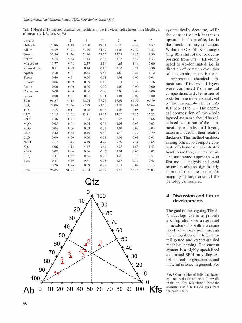
systematically decrease, while the content of Ab increases upwards in the profile, i.e. in the direction of crystallization. Within the Qtz–Ab–Kfs triangle (Fig. 8), a shift of the rock com-position from Qtz + Kfs-domi-nated to Ab-dominated, i.e. in direction of common evolution of leucogranitic melts, is clear.

Approximate chemical com-positions of individual layers were computed from modal compositions and chemistries of rock-forming minerals analyzed by the microprobe (Li by LA-ICP MS) (Tab. 2). The chemi-cal composition of the whole layered sequence should be cal-culated as a mean of the com-positions of individual layers, taken into account their relative thickness. This method enabled, among others, to compute con-tents of chemical elements dif-ficult to analyze, such as boron. The automated approach with fast modal analysis and good textural resolution significantly shortened the time needed for mapping of large areas of the petrological samples.

4. Discussion and future developments

The goal of the ongoing TIMA-X development is to provide a comprehensive automated mineralogy tool with increasing level of automation, through the integration of artificial in-telligence and expert-guided machine learning. The current system is a highly specialized automated SEM providing ex-cellent tool for geosciences and material science in general. For

Tab. 2 Modal and computed chemical compositions of the individual aplite layers from Megiliggar (Cornwall) (vol. % resp. wt. %)

Layer # 1 2 3 4 5 6 7Orthoclase 27.86 18.18 22.60 19.81 11.90 8.39 6.52Albite 16.39 27.94 33.79 34.67 49.02 59.77 72.43Quartz 32.96 35.74 31.16 33.53 25.24 18.97 9.90Schorl 8.14 5.68 7.13 6.36 8.75 8.57 4.33Muscovite 11.77 9.08 2.57 2.10 1.65 1.16 2.00Zinnwaldite 0.11 0.09 0.14 0.15 0.33 0.21 0.30Apatite 0.68 0.81 0.55 0.54 0.60 0.29 1.12Topaz 0.40 0.51 0.00 0.01 0.01 0.00 0.01Fluorite 0.06 0.09 0.09 0.10 0.11 0.12 0.16Rutile 0.00 0.00 0.00 0.02 0.00 0.00 0.00Columbite 0.00 0.00 0.00 0.00 0.00 0.00 0.00Zircon 0.00 0.01 0.01 0.01 0.01 0.02 0.00Sum 98.37 98.13 98.04 97.29 97.62 97.50 96.79SiO2 71.06 73.34 72.99 73.65 70.92 69.41 66.64TiO2 0.15 0.11 0.06 0.06 0.06 0.05 0.04Al2O3 15.15 13.92 13.81 13.07 15.10 16.27 17.22FeOt 1.36 0.97 1.03 0.92 1.25 1.20 0.66MgO 0.05 0.04 0.04 0.04 0.05 0.05 0.03MnO 0.04 0.04 0.03 0.03 0.03 0.02 0.04CaO 0.42 0.52 0.40 0.40 0.46 0.32 0.79Li2O 0.00 0.00 0.00 0.01 0.01 0.01 0.01Na2O 2.17 3.45 4.19 4.27 5.99 7.24 8.65K2O 6.06 4.12 4.17 3.64 2.28 1.63 1.43Rb2O 0.08 0.06 0.06 0.05 0.03 0.02 0.02P2O5 0.31 0.37 0.26 0.26 0.28 0.16 0.51B2O3 0.81 0.56 0.71 0.63 0.87 0.85 0.43F 0.26 0.26 0.09 0.09 0.11 0.09 0.13Sum 96.85 96.95 97.04 96.39 96.46 96.38 96.03

Kfs0 10 20 30 40 50 60 70 80 90 100

Qtz

0

10

20

30

40

50

60

70

80

90

100

Ab

0

10

20

30

40

50

60

70

80

90

100

12

34

7

65

Fig. 8 Composition of individual layers of lined rocks (Megiliggar, Cornwall) in the Ab– Qtz–Kfs triangle. Note the systematic shift to the Ab-apex from the point 1 to 7.


61

further improvements of the AM technology there are still number of topics which can be addressed.

From the instrumentation perspective: further speeding up of data acquisition, and better integration of additional detectors providing extended input of information (Ra-man, WDS, cathodoluminescence, and micro-XRF) might be useful.

From the software perspective: parallelization in data processing and integration of big data concepts could provide significant advantage while working on projects with hundreds or thousands of samples. Also the correla-tive microscopy approach helping to integrate data from other techniques and above-mentioned potential new detectors will be highly beneficial. In the short term, the integration of more sophisticated textural parameters is under development.

Automated classification file construction through the means of artificial intelligence, neural networks, principal component analysis (PCA), machine learning, similar-ity search and hierarchical clustering is also a matter of interest (Hrstka et al. 2017a). The implementation of standards for cross-correlation between different instru-ments would be also highly desirable in the future. This seems particularly important as more AM systems are being developed and there has been very little research comparing their analytical capabilities so far.

5. Conclusions

Combined use of all available signals (mainly BSE and EDS) in conjunction with advanced image and pattern-recognition analysis involving artificial intelligence are required for any modern automated SEM-based mineral analysis system. Such systems can be used not only in their classic domain of mineral processing, plant monitoring, optimization and design but can provide valuable informa-tion in a broad variety of Earth and material sciences. We have demonstrated the high potential of TIMA in extending the everyday tools for geoscience research by a number of case studies. We have also shown that the new generation of automated mineralogy instruments builds on the origi-nal concepts introduced in the early 1970’s but provides additional benefits due to the improvements in analysis modes, full integration of quantitative EDS and availability of computation power and complex programing.

Acknowledgements. We are indebted to Rolando Lastra, Jens Gutzmer, Rogerio Kwitko Ribeiro and the editors for the review. Their comments and suggestions on the manuscript greatly improved the final text. We would also like to thank TESCAN for the support of the TIMA application laboratory at Institute of Geology of the CAS, v. v. i. This study was financed also through Strategie

AV21/4 project and with help of Institute of Geology of the CAS, v. v. i. research plan RVO 67985831. Finally, we would like to thank SGS Minerals for their support of this study.

Electronic supplementary material. Supplementary data on mean atomic numbers of the selected minerals for this paper are available online at the Journal website (http://dx.doi.org/10.3190/ jgeosci.250).

References

Ackerman L, Magna T, Rapprich V, Upadhyay D, Krátký O, Čejková B, Erban V, Kochergina YV, Hrstka T (2017) Contrasting petrogenesis of spatially related carbonatites from Samalpatti and Sevattur, Tamil Nadu, India. Lithos 284: 257–275

Altree-Williams A, Pring A, Ngothai Y, Brugger J (2015) Textural and compositional complexities result-ing from coupled dissolution–reprecipitation reactions in geomaterials. Earth Sci Rev 150: 628–651

Andersen JCØ, Rollinson GK, Snook B, Herrington R, Fairhurst RJ (2009) Use of QEMSCAN® for the char-acterization of Ni-rich and Ni-poor goethite in laterite ores. Miner Eng 22: 1119–1129

Berrezueta E, Ordóñez-Casado B, Bonilla W, Banda R, Castroviejo R, Carrión P, Puglla S (2016) Ore petrography using optical image analysis: application to Zaruma-Portovelo Deposit (Ecuador). Geosciences 6: DOI 10.3390/geosciences6020030

Breiter K, Ďurišová J, Hrstka T, Korbelová Z, Vaňková M, Vašinová Galiová M, Kanický V, Rambousek P, Knésl I, Dobeš P, Dosbaba M (2017) Assessment of magmatic vs. metasomatic processes in rare-metal gran-ites: a case study of the Cínovec/Zinnwald Sn–W–Li deposit, Central Europe. Lithos 292/293: 198–217

Breiter K, Ďurišová J, Hrstka T, Korbelová Z, Vaňková M, Vašinová Galiová M, Müller A, Simons B, Shail RK, Williamson BJ, Davies JA (2018) The transition from granite to banded aplite–pegmatite sheet complexes: an example from Megiliggar Rocks, Tregonning topaz granite, Cornwall. Lithos 302/303: 370–388

Donskoi E, Suthers SP, Fradd SB, Young JM, Campbell JJ, Raynlyn TD, Clout JMF (2007) Utilization of opti-cal image analysis and automatic texture classification for iron ore particle characterisation. Miner Eng 20: 461–471

Fandrich R, Gu Y, Burrows D, Moeller K (2007) Mod-ern SEM-based mineral liberation analysis. Int J Miner Process 84: 310–320

Glagolev AA (1934) Quantitative analysis with the mi-croscope by the point method. Eng Min J 135: 399–400

Gottlieb P (2008) The revolutionary impact of automated mineralogy on mining and mineral processing. In: Wang

http://dx.doi.org/10.3190/jgeosci.250


62

DZ, Sun CY, Wang FL, Zhang LC, Hang L (eds) 24th International Mineral Processing Congress. Science Press, Beijing, pp 165–174

Gottlieb P, Wilkie G, Sutherland D, Ho-Tun E, Suthers S, Perera K, Jenkins B, Spencer S, Butcher A, Rayner J (2000) Using quantitative electron microscopy for pro-cess mineralogy applications. JOM 52: 24–25

Haberlah D, Williams MAJ, Halverson G, McTainsh GH, Hill SM, Hrstka T, Jaime P, Butcher AR, Glasby P (2010) Loess and floods: high-resolution multi-proxy data of Last Glacial Maximum (LGM) slackwater deposi-tion in the Flinders Ranges, semi-arid South Australia. Quat Sci Rev 29:2 673–2693

Haluzová E, Ackerman L, Pašava J, Jonášová Š, Svojtka M, Hrstka T, Veselovský F (2015) Geochronology and characteristics of Ni–Cu–(PGE) mineralization at Rožany, Lusatian Granitoid Complex, Czech Republic. J Geosci 60: 219–236

Harding DP (2002) Mineral identification using a scanning electron microscope. Miner Metall Process 19: 215–219

Harvey PJ, Rouillon M, Dong C, Ettler V, Handley HK, Taylor MP, Tyson E, Tennant P, Telfer V, Trinh R (2017) Geochemical sources, forms and phases of soil contamination in an industrial city. Sci Total Environ 584–585: 505–514

Higgs KE, Haese RR, Golding SD, Schacht U, Watson MN (2015) The Pretty Hill Formation as a natural ana-logue for CO2 storage: an investigation of mineralogical and isotopic changes associated with sandstones exposed to low, intermediate and high CO2 concentrations over geological time. Chem Geol 399: 36–64

Hoal KO, Stammer JG, Appleby SK, Botha J, Ross JK, Botha PW (2009) Research in quantitative mineral-ogy: examples from diverse applications. Miner Eng 22: 402–408

Hrstka T (2008) Preliminary results on the reproducibility of sample preparation and QEMSCAN® measurements for heavy mineral sands samples. Ninth International Congress for Applied Mineralogy, proceedings: ICAM 2008. Australasian Institute of Mining and Metallurgy, Carlton (Vic), pp 107–111

Hrstka T (2012) Paleofluid Chemistry of Orogenic Gold Deposits: Novel Analytical Methods and Case Studies from the Bohemian Massif. Unpublished PhD thesis, Faculty of Science, Charles University in Prague, pp 1–151

Hrstka T, Gottlieb P, Moravec J, Lokoc J (2017a) The future of SEM-based automated mineralogy and artifi-cial intelligence in applied mineralogy. Sci Res Abstr 6: Digilabs, pp 42

Hrstka T, Motl D, Gottlieb P, Hladil J (2017b) Using an automated approach in building a dust particle atlas for research and environmental monitoring. Sci Res Abstr 6: Digilabs pp 43

Johnson C, Pownceby MI, Wilson NC (2015) The appli-cation of automated electron beam mapping techniques to the characterisation of low grade, fine-grained min-eralisation; potential problems and recommendations. Miner Eng 79: 68–83

Jordens A, Marion C, Grammatikopoulos T, Waters KE (2016) Understanding the effect of mineralogy on muscovite flotation using QEMSCAN. Int J Miner Pro-cess 155: 6–12

Knappett C, Pirrie D, Power MR, Nikolakopoulou I, Hilditch J, Rollinson GK (2011) Mineralogical analysis and provenancing of ancient ceramics using automated SEM-EDS analysis (QEMSCAN®): a pilot study on LB I pottery from Akrotiri, Thera. J Archaeolog Sci 38: 219–232

Kwitko-Ribeiro R (2012) New sample preparation de-velopments to minimize mineral segregation in process mineralogy. In: Broekmans MATM (ed) Proceedings of the 10th International Congress of Applied Mineralogy. Springer, Berlin, Heidelberg, pp 411–417

Lane GR, Martin C, Pirard E (2008) Techniques and ap-plications for predictive metallurgy and ore characteriza-tion using optical image analysis. Miner Eng 21: 568–577

Larrea ML, Castro SM, Bjerg EA (2014) A software solution for point counting. Petrographic thin section analysis as a case study. Arabian J Geosci 7: 2981–2989

Lastra R (2007) Seven practical application cases of libera-tion analysis. Int J Miner Process 84: 337–347

Lastra R, Paktunc D (2016) An estimation of the variabil-ity in automated quantitative mineralogy measurements through inter-laboratory testing. Miner Eng 95: 138–145

Le Bas MJ, Streckeisen AL (1991) The IUGS systemat-ics of igneous rocks. J Geol Soc, London 148: 825–833

Le Maitre RW (2002) Igneous Rocks: A Classification and Glossary of Terms. Cambridge University Press, Cambridge, pp 1–236

Lloyd GE (1987) Atomic number and crystallographic contrast images with the SEM: a review of backscattered electron techniques. Mineral Mag 51: 3–19

London D (2008) Pegmatites. Canad Mineral, Spec Publ 10: pp 1–347

Lotter NO, Kormos LJ, Oliveira J, Fragomeni D, White-man E (2011) Modern process mineralogy: two case studies. Miner Eng 24: 638–650

Mineralogical database (2017) Mineralogical database. Accessed on May 10, 2017 at http://www.webmineral.com

Motl D, Filip V (2013) Method and apparatus for material analysis by a focused electron beam using character-istic X-rays and back-scattered electrons. (Patent no. WO2017050303 A1)

Müller A, Breiter K, Seltmann R, Pécskay Z (2005) Quartz and feldspar zoning in the eastern Erzgebirge volcano–plutonic complex (Germany, Czech Republic): evidence of multiple magma mixing. Lithos 80: 201–227


63

Neumannová K, Thér R, Květina P, Hrstka T (2016) Perception of technological variability on the example of Neolithic settlement site in Bylany. Praehistorica 33: 291–306 (in Czech)

Nie J, Peng W (2014) Automated SEM–EDS heavy mineral analysis reveals no provenance shift between glacial loess and interglacial paleosol on the Chinese Loess Plateau. Aeolian Res 13: 71–75

Pérez-Barnuevo L, Pirard E, Castroviejo R (2013) Automated characterisation of intergrowth textures in mineral particles. A case study. Miner Eng 52: 136–142

Pirard E (2004) Multispectral imaging of ore minerals in optical microscopy. Mineral Mag 68: 323–333

Pirrie D, Rollinson GK (2011) Unlocking the applications of automated mineral analysis. Geol Today 27: 226–235

Poliakov A, Donskoi E (2014) Automated relief-based discrimination of non-opaque minerals in optical image analysis. Miner Eng 55: 111–124

Pooler R, Dold B (2017) Optimization and quality control of automated quantitative mineralogy analysis for acid rock drainage prediction. Minerals 7: DOI 10.3390/min7010012

Rollinson GK, Andersen JCØ, Stickland RJ, Boni M, Fairhurst R (2011) Characterisation of non-sulphide zinc deposits using QEMSCAN®. Miner Eng 24: 778–787

Sandmann D, Gutzmer J (2013) Use of mineral liberation analysis (MLA) in the characterization of lithium-bearing micas. J Miner Mater Charact Eng 1: 285–292

Sandmann D, Gutzmer J (2015) Nature and distribution of PGE mineralization in gabbroic rocks of the Lusatian Block, Saxony, Germany. Z Geol Wiss 166: 35–53

Sánchez E, Deluigi MT, Castellano G (2012) Mean atomic number quantitative assessment in backscattered electron imaging. Microsc Microanal 18: 1355–1361

Santoro L, Boni M, Rollinson GK, Mondillo N, Balas-sone G, Clegg AM (2014) Mineralogical characteriza-tion of the Hakkari nonsulfide Zn(Pb) deposit (Turkey): the benefits of QEMSCAN®. Miner Eng 69: 29–39

Santoro L, Rollinson GK, Boni M, Mondillo N (2015) Automated Scanning Electron Microscopy QEMSCAN®-based mineral identification and quantification of the Jabali Zn–Pb–Ag nonsulphide deposit (Yemen). Econ Geol 110: 1083–1099

Slavík L, Valenzuela-Ríos JI, Hladil J, Chadimová L, Liao JC, Hušková A, Calvo H, Hrstka T (2016) Warming or cooling in the Pragian? Sedimentary record and petrophysical logs across the Lochkovian–Pragian boundary in the Spanish Central Pyrenees. Palaeogeogr Palaeoclimatol Palaeoecol 449: 300–320

Smith DGW, Nickel EH (2008) Codification of unnamed minerals. J Petrol 49: 581–583

Smythe DM, Lombard A, Coetzee LL (2013) Rare Earth Element deportment studies utilising QEMSCAN tech-nology. Miner Eng 52: 52–61

Stone M (1969) Nature and origin of banding in the granitic sheets Tremearne, Porthleven, Cornwall. Geol Mag 106: 142–158

Svojtka M, Ackerman L, Medaris LG, Hegner E, Valley JW, Hirajima T, Jelínek E, Hrstka T (2016) Petrologi-cal, geochemical and Sr–Nd–O isotopic constraints on the origin of garnet and spinel pyroxenites from the Moldanubian Zone of the Bohemian Massif. J Petrol 57: 897–920

Štemprok M (2016) Drill hole CS-1 penetrating the Cí-novec/Zinnwald granite cupola (Czech Republic): an A-type granite with important hydrothermal mineraliza-tion. J Geosci 61: 395–423

Štemprok M, Šulcek Z (1969) Geochemical profile through an ore-bearing lithium granite. Econ Geol 64: 392–404

Ward I, Merigot K, McInnes BIA (2018) Application of Quantitative Mineralogical Analysis in archaeological micromorphology: a case study from Barrow Is., Western Australia. J Archaeol Method Theory 25: 45–68

Whitney JA, Stormer JC (1977) The distribution of NaAl-Si3O8 between coexisting microcline and plagioclase and its effect on geothermometric calculations. Amer Miner 62: 687–691

Whitney DL, Evans BW (2010) Abbreviations for names of rock-forming minerals. Amer Miner 95: 185–187

Žák K, Skála R, Řanda Z, Mizera J, Heissig K, Acker-man L, Ďurišová J, Jonášová Š, Kameník J, Magna T (2016) Chemistry of Tertiary sediments in the sur-roundings of the Ries impact structure and moldavite formation revisited. Geochim Cosmochim Acta 179: 287–311

Documents

Original paper Automated mineralogy and petrology ... · The collection of representative modal mineralogy data as well as textural and chemical information on statistically ... mineralogy,