ORIGINAL ARTICLE - University of California, San Diegomaeresearch.ucsd.edu/tartakovsky/Papers/marasco-2014-vegetation.pdfORIGINAL ARTICLE Vegetation Pattern ... DMT was supported in

Bull Math Biol (2014) 76:2866–2883DOI 10.1007/s11538-014-0036-6

ORIGINAL ARTICLE

Vegetation Pattern Formation Due to InteractionsBetween Water Availability and Toxicity in Plant–SoilFeedback

Addolorata Marasco · Annalisa Iuorio · Fabrizio Cartení ·Giuliano Bonanomi · Daniel M. Tartakovsky · Stefano Mazzoleni ·Francesco Giannino

Received: 11 March 2014 / Accepted: 2 October 2014 / Published online: 23 October 2014© Society for Mathematical Biology 2014

Abstract Development of a comprehensive theory of the formation of vegetation pat-terns is still in progress. A prevailing view is to treat water availability as the maincausal factor for the emergence of vegetation patterns. While successful in capturingthe occurrence of multiple vegetation patterns in arid and semiarid regions, this hypoth-esis fails to explain the presence of vegetation patterns in humid environments. We

Electronic supplementary material The online version of this article (doi:10.1007/s11538-014-0036-6)contains supplementary material, which is available to authorized users.

AI was partially supported by the FWF doctoral program “Dissipation and dispersion in nonlinear PDEs”funded under grant W1245. FC was supported by POR Campania FSE 20072013, Project CARINA.DMT was supported in part by the grants from Air Force Office of Scientific Research(DE-FG02-07ER25815) and National Science Foundation (EAR-1246315).

A. MarascoDepartment of Mathematics and Applications “R. Caccioppoli”, University of Naples Federico II,Via Cintia 80126, Naples, Italye-mail: [email protected]

A. IuorioInstitute for Analysis and Scientific Computing, Vienna University of Technology,Wiedner Hauptstraße 8-10, 1040 Vienna, Austriae-mail: [email protected]

F. Cartení · G. Bonanomi · S. Mazzoleni · F. Giannino (B)Department of Agriculture, University of Naples Federico II,Via Università 100, 80055 Portici (Na), Italye-mail: [email protected]

F. Carteníe-mail: [email protected]

G. Bonanomie-mail: [email protected]

123

http://dx.doi.org/10.1007/s11538-014-0036-6

Effect of Toxicity on Vegetation Pattern Formation 2867

explore the rich structure of a toxicity-mediated model of the vegetation pattern for-mation. This model consists of three PDEs accounting for a dynamic balance betweenbiomass, water, and toxic compounds. Different (ecologically feasible) regions of themodel’s parameter space give rise to stable spatial vegetation patterns in Turing andnon-Turing regimes. Strong negative feedback gives rise to dynamic spatial patternsthat continuously move in space while retaining their stable topology.

Keywords Turing pattern · Negative feedback · Bifurcation analysis ·Numerical simulations

1 Introduction

The occurrence of regular vegetation patterns has been studied by plant ecologists fora long time (Watt 1947; White 1971). Different patterns, such as spots, labyrinths,gaps, and stripes, as well as plant rings and fungal fairy rings (Valentin et al. 1999;Bonanomi et al. 2012, 2013), occur in a variety of natural environments (Boale andHodge 1964; Wickens and Collier 1971; Leprun 1999; Okayasu and Aizawa 2001).It has been hypothesized that their development is affected by global phenomena likeclimate change (Rietkerk et al. 2002; Dekker et al. 2009). An extensive analysis of datafrom 249 geographical locations supports this hypothesis by correlating the observedregular vegetation patterns with climatic variables and soil properties (Deblauwe et al.2008). Such studies suggest that vegetation patterns in arid and semiarid environmentsmight provide early warning signs of climate shifts and critical transitions (van deKoppel et al. 1997; Rietkerk et al. 1997, 2004; Scheffer et al. 2009).

Development of a comprehensive theory of the formation of vegetation patterns isstill in progress. Phenomenological models of Lefever and Lejeune (1997) and Lejeuneet al. (1999, 2002) postulate two feedback mechanisms of pattern formation: short-range facilitation of plants under their aerial structures and long-range competitionbetween plants by overlapping root zones. A more prevailing theory identifies wateravailability as the main causal factor for the emergence of vegetation patterns. Itis usually formulated in terms of two coupled partial differential equations (PDEs)governing the dynamics of plant biomass and (surface or soil) water (Klausmeier1999; Hardenberg et al. 2001; Rietkerk et al. 2002; Meron et al. 2004; Ursino andContarini 2006; Gilad et al. 2007a, b; Kealy and Wollkind 2012; Nathan et al. 2013).In these and other similar models, vegetation patterns emerge solely due to a feedbackbetween biomass and water (e.g., water infiltration and/or evaporation, plant wateruptake, and surface water runoff). Treating water availability as the only controlling

S. Mazzolenie-mail: [email protected]

D. M. TartakovskyDepartment of Mechanical and Aerospace Engineering, University of California, San Diego,9500 Gilman Drive, La Jolla, CA 92093, USAe-mail: [email protected]

123

2868 A. Marasco et al.

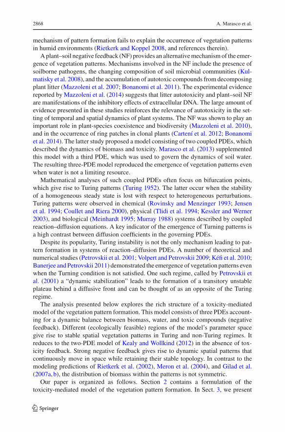
mechanism of pattern formation fails to explain the occurrence of vegetation patternsin humid environments (Rietkerk and Koppel 2008, and references therein).

A plant–soil negative feedback (NF) provides an alternative mechanism of the emer-gence of vegetation patterns. Mechanisms involved in the NF include the presence ofsoilborne pathogens, the changing composition of soil microbial communities (Kul-matisky et al. 2008), and the accumulation of autotoxic compounds from decomposingplant litter (Mazzoleni et al. 2007; Bonanomi et al. 2011). The experimental evidencereported by Mazzoleni et al. (2014) suggests that litter autotoxicity and plant–soil NFare manifestations of the inhibitory effects of extracellular DNA. The large amount ofevidence presented in these studies reinforces the relevance of autotoxicity in the set-ting of temporal and spatial dynamics of plant systems. The NF was shown to play animportant role in plant-species coexistence and biodiversity (Mazzoleni et al. 2010),and in the occurrence of ring patches in clonal plants (Cartení et al. 2012; Bonanomiet al. 2014). The latter study proposed a model consisting of two coupled PDEs, whichdescribed the dynamics of biomass and toxicity. Marasco et al. (2013) supplementedthis model with a third PDE, which was used to govern the dynamics of soil water.The resulting three-PDE model reproduced the emergence of vegetation patterns evenwhen water is not a limiting resource.

Mathematical analyses of such coupled PDEs often focus on bifurcation points,which give rise to Turing patterns (Turing 1952). The latter occur when the stabilityof a homogeneous steady state is lost with respect to heterogeneous perturbations.Turing patterns were observed in chemical (Rovinsky and Menzinger 1993; Jensenet al. 1994; Coullet and Riera 2000), physical (Tlidi et al. 1994; Kessler and Werner2003), and biological (Meinhardt 1995; Murray 1988) systems described by coupledreaction–diffusion equations. A key indicator of the emergence of Turning patterns isa high contrast between diffusion coefficients in the governing PDEs.

Despite its popularity, Turing instability is not the only mechanism leading to pat-tern formation in systems of reaction–diffusion PDEs. A number of theoretical andnumerical studies (Petrovskii et al. 2001; Volpert and Petrovskii 2009; Kéfi et al. 2010;Banerjee and Petrovskii 2011) demonstrated the emergence of vegetation patterns evenwhen the Turning condition is not satisfied. One such regime, called by Petrovskii etal. (2001) a “dynamic stabilization” leads to the formation of a transitory unstableplateau behind a diffusive front and can be thought of as an opposite of the Turingregime.

The analysis presented below explores the rich structure of a toxicity-mediatedmodel of the vegetation pattern formation. This model consists of three PDEs account-ing for a dynamic balance between biomass, water, and toxic compounds (negativefeedback). Different (ecologically feasible) regions of the model’s parameter spacegive rise to stable spatial vegetation patterns in Turing and non-Turing regimes. Itreduces to the two-PDE model of Kealy and Wollkind (2012) in the absence of tox-icity feedback. Strong negative feedback gives rise to dynamic spatial patterns thatcontinuously move in space while retaining their stable topology. In contrast to themodeling predictions of Rietkerk et al. (2002), Meron et al. (2004), and Gilad et al.(2007a, b), the distribution of biomass within the patterns is not symmetric.

Our paper is organized as follows. Section 2 contains a formulation of thetoxicity-mediated model of the vegetation pattern formation. In Sect. 3, we present

123


Fig. 1 A soil–plant–atmospheresystem accounts for thefeedback between plant biomass(B), toxic compounds (T ), andsoil water (W ). The continuouslines represent transfers ofmatter between thecompartments, while the dashedlines represent the influences

B

T W

litte

rfal

l

uptake prec

ipit

atio

n

evap

orat

ion

decay

simulation results representative of an ecologically feasible range of the model para-meters. A linear stability analysis of the model’s homogenous stationary solutions toboth homogeneous and inhomogenous perturbations is presented in Sect. 4. A discus-sion of ecological implications of the toxicity-mediated model is presented in Sect. 5.

2 Mathematical Model

Following Cartení et al. (2012) and Marasco et al. (2013), we postulate that vegetationpatterns emerge as a result of the competition between biomass B (kg/m2), water W(kg/m2), and toxic compounds T (kg/m2). Figure 1 provides a schematic representa-tion of the interactions between these three quantities at any spatial point x = (x, y)�and time t : Growth of biomass B is mediated by water availability, its intrinsic mor-tality, and the toxic compounds; availability of water W is affected by precipitation,evaporation, and transpiration (plant water uptake); and toxic compounds T are pro-duced by the decomposition of dead plants and removed from the soil by intrinsicdegradation and precipitation.

These processes are described by a system of coupled PDEs

∂ B

∂t= DB∇2 B + fB(B, W, T ), fB ≡ cB2W − (d + sT )B; (1a)

∂W

∂t= DW ∇2W + fW (B, W ), fW = p − r B2W − lW ; (1b)

∂T

∂t= fT (B, T ), fT = q(d + sT )B − (k + wp)T (1c)

where the real positive constants DB and DW represent dispersal and effective diffusioncoefficients of biomass and water, respectively. Their values, as well as those of modelparameters c > 0, d > 0, p > 0, q > 0, r > 0, l > 0, s ≥ 0, w ≥ 0 and k ≥ 0,are either chosen in accordance with Klausmeier (1999) and Cartení et al. (2012) or

123


Table 1 Model parameters and their values

Parameter Description Units Values

c Growth rate of B due to water uptake m4 d−1 kg−2 0.002

d Death rate of biomass B d−1 0.01

k Decay rate of toxicity T d−1 0.01 or 0.2

l Water loss due to evaporation and drainage d−1 0.01

p Precipitation rate kg d−1 m−2 [0, 2]q Proportion of toxins in dead biomass – 0.05

r Rate of water uptake m4 d−1 kg−2 0.35

s Sensitivity of plants to toxicity T m2 d−1 kg−1 0 or 0.2

w Washing out of toxins by precipitation kg day−2 m−2 0.001

DB “Diffusion coefficient” for biomass m2 d−1 0.01

DW “Diffusion coefficient” for water m2 d−1 0.8

selected from within an order-of-magnitude feasibility range. They are summarizedin Table 1. Equations (1) are defined on the bounded domain Ω = {0 ≤ x ≤ Lx , 0 ≤y ≤ L y} and are subject to the boundary and initial conditions

∂n B = 0, ∂nW = 0, ∂nT = 0, x ∈ ∂Ω, t ≥ 0 (2a)

and

B(x, 0) = B0(x), W (x, 0) = W0(x), T (x, 0) = 0, x ∈ Ω (2b)

where ∂Ω is the boundary of Ω; ∂n is the normal derivative on ∂Ω; B0 and W0 areinitial spatial distributions of biomass and water, respectively.

Three-equation model (1) accounts for the negative soil–plant feedback due to planttoxicity that is absent in the two-equation models of Klausmeier (1999) and Kealyand Wollkind (2012). The latter two models attribute the occurrence of vegetationpatterns solely to competition between biomass growth and water availability. Settings = 0 in (1) decouples pattern formation from the effects of toxicity and reducesthe structure of our model to that introduced by Kealy and Wollkind (2012). It isworthwhile emphasizing that their simulations and analysis were carried out for aninfinite domain, while we define our model on bounded domain Ω .

3 Pattern Formation: Simulation Results

The simulations reported below are performed on a square lattice of 100 × 100 ele-ments, with initial biomass B0 = 0.2 in N0 = 5,000 randomly selected elements(or the total initial biomass Btot

0 = 1,000) and B0 = 0 in the remaining nodes. Thesimulation time tmax = 274 years consists of 100,000 time steps Δt = 0.01 days.In all simulations, eight of the eleven dimensional model parameters (i.e., two out of

123


s=

0an

yk

s=

0.2 k

=0.

2k

=0.

01p = 0.4 p = 0.6 p = 0.8 p = 1.0 p = 1.1 p = 1.2 p = 2.0

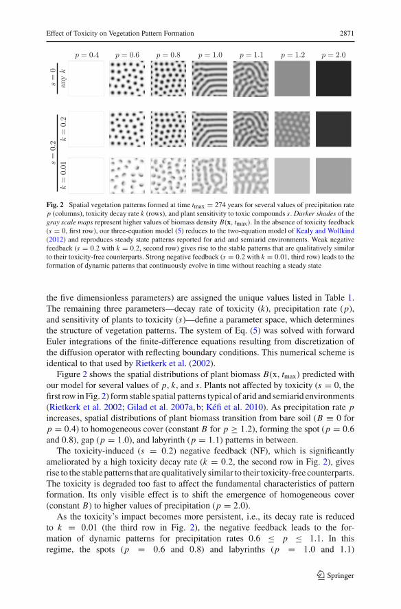
Fig. 2 Spatial vegetation patterns formed at time tmax = 274 years for several values of precipitation ratep (columns), toxicity decay rate k (rows), and plant sensitivity to toxic compounds s. Darker shades of thegray scale maps represent higher values of biomass density B(x, tmax). In the absence of toxicity feedback(s = 0, first row), our three-equation model (5) reduces to the two-equation model of Kealy and Wollkind(2012) and reproduces steady state patterns reported for arid and semiarid environments. Weak negativefeedback (s = 0.2 with k = 0.2, second row) gives rise to the stable patterns that are qualitatively similarto their toxicity-free counterparts. Strong negative feedback (s = 0.2 with k = 0.01, third row) leads to theformation of dynamic patterns that continuously evolve in time without reaching a steady state

the five dimensionless parameters) are assigned the unique values listed in Table 1.The remaining three parameters—decay rate of toxicity (k), precipitation rate (p),and sensitivity of plants to toxicity (s)—define a parameter space, which determinesthe structure of vegetation patterns. The system of Eq. (5) was solved with forwardEuler integrations of the finite-difference equations resulting from discretization ofthe diffusion operator with reflecting boundary conditions. This numerical scheme isidentical to that used by Rietkerk et al. (2002).

Figure 2 shows the spatial distributions of plant biomass B(x, tmax) predicted withour model for several values of p, k, and s. Plants not affected by toxicity (s = 0, thefirst row in Fig. 2) form stable spatial patterns typical of arid and semiarid environments(Rietkerk et al. 2002; Gilad et al. 2007a, b; Kéfi et al. 2010). As precipitation rate pincreases, spatial distributions of plant biomass transition from bare soil (B ≡ 0 forp = 0.4) to homogeneous cover (constant B for p ≥ 1.2), forming the spot (p = 0.6and 0.8), gap (p = 1.0), and labyrinth (p = 1.1) patterns in between.

The toxicity-induced (s = 0.2) negative feedback (NF), which is significantlyameliorated by a high toxicity decay rate (k = 0.2, the second row in Fig. 2), givesrise to the stable patterns that are qualitatively similar to their toxicity-free counterparts.The toxicity is degraded too fast to affect the fundamental characteristics of patternformation. Its only visible effect is to shift the emergence of homogeneous cover(constant B) to higher values of precipitation (p = 2.0).

As the toxicity’s impact becomes more persistent, i.e., its decay rate is reducedto k = 0.01 (the third row in Fig. 2), the negative feedback leads to the for-mation of dynamic patterns for precipitation rates 0.6 ≤ p ≤ 1.1. In thisregime, the spots (p = 0.6 and 0.8) and labyrinths (p = 1.0 and 1.1)

123


s=

0an

yk

s=

0.2 k

=0.

2k

=0.

01p = 0.4 p = 0.6 p = 0.8 p = 1.0 p = 1.1 p = 1.2 p = 2.0

Fig. 3 Temporal evolution of biomass density B(xc, t) at the central pixel of the simulation domain (blackline) and of the biomass density Bave(t) averaged over the entire lattice (gray line), for several values ofprecipitation rate p (columns), toxicity decay rate k (rows), and plant sensitivity to toxic compounds s.The time t on the horizontal axis varies from 0 to tmax = 274 years, with 100,000 time steps. The lack of(s = 0, first row) or weak (s = 0.2 with k = 0.2, second row) toxicity-induced negative feedback results instable steady state asymptotes after exhibiting transitory fluctuations at early times. Strong toxicity-inducednegative feedback (s = 0.2 with k = 0.01 and 0.6 ≤ p ≤ 1.1, third row) gives rise to persistent temporalfluctuations of B(xc, t), indicating that vegetation patterns continue to evolve without reaching a stablespatial configuration

continuously evolve in time, without reaching a steady state (see also the Supple-mentary Material, SPOT_k=0.01_p=0.6.avi, LABYRINTH_k=0.01_p=1.0.avi andGAP_k=0.01_p=1.1.avi). This dynamic behavior represents the biomass “escapingfrom the toxicity” that accumulates in the soil patches previously occupied by thevegetation.

Figure 3 elucidates this phenomenon by exhibiting the temporal evolution of bothbiomass B(xc, t) at the central pixel (black line) and the average biomass of the entirelattice Bave(t) (gray line). The lack of (s = 0, first row) or weak (s = 0.2 withk = 0.2, second row) toxicity-induced negative feedback results in stable steadystate asymptotes Bst(xc) after exhibiting transitory fluctuations at early times. Forbare soil (first column) and uniform cover (last column), the biomass values Bst(xc)

coincide with the average values Bave(tmax). This stable behavior is in sharp contrast tothe persistent temporal fluctuations of B(xc, t) introduced by strong toxicity-inducednegative feedback (s = 0.2 with k = 0.01 and 0.6 ≤ p ≤ 1.1, third row). In thisregime, the biomass density B(xc, t) oscillates indefinitely, i.e., vegetation patternscontinue to evolve without reaching a stable spatial configuration (see also videos inthe Supplementary Material).

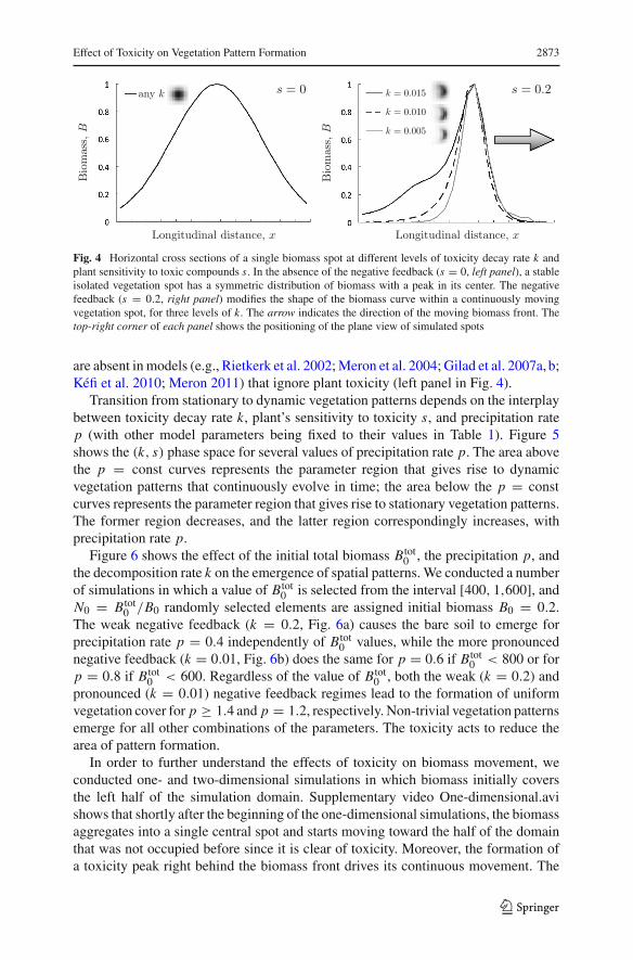
Our model predicts asymmetric distributions of biomass within individual spotsand stripes (Fig. 4). The biomass peak within each spot is shifted toward the directionof the spot’s movement, escaping the zone with the highest toxicity accumulation.The degree of asymmetry increases as toxicity decay rate k decreases (right panel inFig. 4). The biomass distribution exhibits a tail on the side opposite to the direction ofthe spot’s movement. The length of this tail depends on the persistence of toxicity inthe soil: Low values of k result in a short biomass tail due to the high toxicity left in thepreviously occupied soil, while higher k values degrade the soil toxicity and allow alarger portion of biomass to persist in the tail. Such asymmetric biomass distributions

123


s = 0any k

Longitudinal distance, x

Bio

mas

s,B

Bio

mas

s,B

Longitudinal distance, x

s = 0.2k = 0.015

k = 0.010

k = 0.005

Fig. 4 Horizontal cross sections of a single biomass spot at different levels of toxicity decay rate k andplant sensitivity to toxic compounds s. In the absence of the negative feedback (s = 0, left panel), a stableisolated vegetation spot has a symmetric distribution of biomass with a peak in its center. The negativefeedback (s = 0.2, right panel) modifies the shape of the biomass curve within a continuously movingvegetation spot, for three levels of k. The arrow indicates the direction of the moving biomass front. Thetop-right corner of each panel shows the positioning of the plane view of simulated spots

are absent in models (e.g., Rietkerk et al. 2002; Meron et al. 2004; Gilad et al. 2007a, b;Kéfi et al. 2010; Meron 2011) that ignore plant toxicity (left panel in Fig. 4).

Transition from stationary to dynamic vegetation patterns depends on the interplaybetween toxicity decay rate k, plant’s sensitivity to toxicity s, and precipitation ratep (with other model parameters being fixed to their values in Table 1). Figure 5shows the (k, s) phase space for several values of precipitation rate p. The area abovethe p = const curves represents the parameter region that gives rise to dynamicvegetation patterns that continuously evolve in time; the area below the p = constcurves represents the parameter region that gives rise to stationary vegetation patterns.The former region decreases, and the latter region correspondingly increases, withprecipitation rate p.

Figure 6 shows the effect of the initial total biomass Btot0 , the precipitation p, and

the decomposition rate k on the emergence of spatial patterns. We conducted a numberof simulations in which a value of Btot

0 is selected from the interval [400, 1,600], andN0 = Btot

0 /B0 randomly selected elements are assigned initial biomass B0 = 0.2.The weak negative feedback (k = 0.2, Fig. 6a) causes the bare soil to emerge forprecipitation rate p = 0.4 independently of Btot

0 values, while the more pronouncednegative feedback (k = 0.01, Fig. 6b) does the same for p = 0.6 if Btot

0 < 800 or forp = 0.8 if Btot

0 < 600. Regardless of the value of Btot0 , both the weak (k = 0.2) and

pronounced (k = 0.01) negative feedback regimes lead to the formation of uniformvegetation cover for p ≥ 1.4 and p = 1.2, respectively. Non-trivial vegetation patternsemerge for all other combinations of the parameters. The toxicity acts to reduce thearea of pattern formation.

In order to further understand the effects of toxicity on biomass movement, weconducted one- and two-dimensional simulations in which biomass initially coversthe left half of the simulation domain. Supplementary video One-dimensional.avishows that shortly after the beginning of the one-dimensional simulations, the biomassaggregates into a single central spot and starts moving toward the half of the domainthat was not occupied before since it is clear of toxicity. Moreover, the formation ofa toxicity peak right behind the biomass front drives its continuous movement. The

123


Toxicity decay rate, k

Sens

itiv

ity

toto

xici

ty,s

Fig. 5 (k, s) phase space for several values of precipitation rate p. The area above the p = const curvesrepresents the parameter region that gives rise to dynamic vegetation patterns, which continuously evolvein time; the area below the p = const curves represents the parameter region that gives rise to stationaryvegetation patterns. The former region decreases, and the latter region correspondingly increases, withprecipitation rate p. The curves are obtained with numerical simulations in which the (k, s) space isdiscretized by the 25 × 41 elements

Fig. 6 Effect of precipitation rate p, initial biomass B0, and decomposition rate k on pattern formation.The panels k = 0.2 (a) and k = 0.01 (b) show the emerged spatial pattern as a function of precipitationrate (0.4 ≤ p ≤ 2.0) and of initial value of the biomass B. White, gray, and black zones correspond to baresoil, vegetation pattern (i.e., spot, labyrinth, or gaps), and homogeneous vegetation, respectively

two-dimensional biomass dynamics is reflected in its temporal snapshots in Fig. 7.Shortly after the beginning of the simulation, the biomass in the left half of the domainstarts to decrease, giving rise to a biomass front invading the empty half of the domainthat is clear of toxic compounds (second column in Fig. 7). A toxicity peak is formedright behind the biomass front (third column in Fig. 7); it forces the front to keeptraveling in the same direction and impedes the diffusion of biomass to the left. Afterthe first front, the residual biomass in the left part of the domain starts creating newtraveling fronts (fourth column in Fig. 7) until the vertical symmetry is broken and thelinear fronts become continuously moving spots (fifth column in Fig. 7).

123


2-d

map

sTra

nsec

tst = 1 t = 100 t = 800 t = 4000 t = 9000

BWT

Fig. 7 Temporal evolution of the system starting from homogeneous biomass cover in the left half of thesimulation domain. The first row panels show two-dimensional maps of the biomass density. The secondrow panels represent plots of B, W , and T along the central horizontal transect of the domain. Parametervalues are set to p = 0.8, s = 0.2, and k = 0.01

4 Pattern Formation: Linear Stability Analysis

Systematic analysis of mathematical properties of ecological problems consisting ofmore than two PDEs is notoriously challenging (Sherratt 2005; Sherratt and Lord2007; Sherratt 2010). Quasi-steady state approximations, which are often employedto perform stability analyses and to verify the presence of Turing bifurcations, arebased on the phenomenological assumption that the dynamics of one state variable ismuch faster than those of the others (HilleRisLambers et al. 2001; Kéfi et al. 2010).Since this approach presents some drawbacks in the context of vegetation modeling(Flach and Schnell 2006), we do not adopt it here.

The subsequent analysis is facilitated by transforming model (1) into its dimen-sionless form. Let us introduce dimensionless independent and dependent variables

x̃ =√

k

DWx, t̃ = kt, B̃ = kr

cpB, W̃ = k

pW, T̃ = kr

cpqT (3)

and corresponding dimensionless parameters

μ = DB

DW, α = d

k + wp, β = α2cpsq

d2r, γ = α3c2 p2

d3r, λ = αl

d. (4)

Then, Eq. (1) take a dimensionless form (unless otherwise noted we omit the tildes)

∂ B

∂t= μ∇2 B + fB(B, W, T ), fB ≡ γ B2W − (α + βT )B; (5a)

∂W

∂t= ∇2W + fW (B, W, T ), fW = 1 − γ B2W − λW ; (5b)

∂T

∂t= fT (B, W, T ), fT = αB − (1 − βB)T . (5c)

123


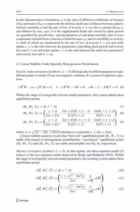
In this dimensionless formulation, μ is the ratio of diffusion coefficients of biomass(DB) and water (DW ); α represents the intrinsic death rate (a balance between a plant’sintrinsic mortality d and the rate of loss of toxicity k + wp due to natural decay, k,and dilution by rain, wp); β is the supplemental death rate caused by plant growth(as quantified by growth rate c and precipitation p) and plant mortality (due to toxiccompounds released from a fraction of dead biomass, q, and its sensibility to toxicity,s), both of which are ameliorated by the rate of loss of toxicity k + wp and wateruptake r ; γ is the ratio between the parameters controlling plant growth and toxicityloss rate k + wp and water uptake r ; λ is the ratio between the water loss parameter land toxicity loss rate k + wp.

4.1 Linear Stability Under Spatially Homogeneous Perturbations

Toxicity-induced negative feedback (s > 0). Biologically feasible homogeneous equi-librium points of model (5) are non-negative solutions of a system of algebraic equa-tions

γ B2W − (α + βT )B = 0, 1 − γ B2W − λW = 0, αB − (1 − βB)T = 0. (6)

Within the range of ecologically relevant model parameters, this system admits threeequilibrium points,

(B1, W1, T1) = (0, λ−1, 0) (7)

(B2, W2, T2) =(

γ + Δ

2(α + β)γ,

2(α + β)βλ + γ − Δ

2λ(β2λ + γ ),−2αβλ + γ + Δ

2(β2λ + γ )

)(8)

(B3, W3, T3) =(

γ − Δ

2(α + β)γ,

2(α + β)βλ + γ + Δ

2λ(β2λ + γ ),−2αβλ + γ + Δ

2(β2λ + γ )

)(9)

where Δ ≡ √γ [γ − 4(α + β)αλ] introduces a constraint γ ≥ 4(α + β)αλ.

A linear stability analysis reveals that “bare-soil” equilibrium point (B1, W1, T1) isstable with respect to homogeneous perturbations; “coexistence” equilibrium points(B2, W2, T2) and (B3, W3, T3) are stable and unstable (see Fig. 8), respectively.

Absence of negative feedback (s = 0). In this regime, our three-equation model (5)reduces to the two-equation model analyzed by Kealy and Wollkind (2012). Withinthe range of ecologically relevant model parameters, the resulting system admits threeequilibrium points,

(B01 , W 0

1 , T 01 ) = (0, λ−1, 0) (10)

(B02 , W 0

2 , T 02 ) =

(γ + √

γ 2 − 4α2λγ

2αγ,

α

γ B02

, αB02

)(11)

(B03 , W 0

3 , T 03 ) =

(γ − √

γ 2 − 4α2λγ

2αγ,

α

γ B03

, αB03

)(12)

123


Bio

mas

s,B

Precipitation rate, p

p∗pS

(a) s �= 0, k = 0.01


p∗pS

Bio

mas

s,B

(b) s �= 0, k = 0.2

Fig. 8 Bifurcation diagram for homogeneous stationary solutions of (5) showing biomass B versus pre-cipitation rate p in the presence of negative feedback (s = 0.2) for k = 0.01 (a) and k = 0.2 (b). Thedotted lines denote stable equilibria of the spatial and non-spatial model. Continuous lines denote unstableequilibria for the spatially homogeneous case. The dashed lines denote equilibria which are asymptoticallystable to spatially homogeneous perturbations but unstable to heterogeneous perturbations. The verticallines p = p∗ and p = pS delineate the region of a Turing bifurcation; the values of p∗ and pS are givenby Eq. (15). Two non-trivial equilibria (i.e., uniform vegetation) exist for p > p∗. Spatial bistability occurswhen p ≥ pS

Bio

mas

s,B

p∗pS


(c) s = 0, any k

Fig. 9 Bifurcation diagram for homogeneous stationary solutions of (5) showing biomass B versus pre-cipitation rate p in the absence of negative feedback (s = 0). The dotted lines denote stable equilibria ofthe spatial and non-spatial model. The continuous lines denote unstable equilibria for the spatially homo-geneous case. The dashed lines denote equilibria which are asymptotically stable to spatially homogeneousperturbations but unstable to heterogeneous perturbations. Spatial bistability occurs when p ≥ pS

with a parameter constraint γ ≥ 4α2λ. This result is identical to that given by Eqs. (4)and (5) in Kealy and Wollkind (2012). A linear stability analysis suggests that bare-soil equilibrium point (B0

1 , W 01 , T 0

1 ) is stable with respect to homogeneous pertur-bations; “coexistence” equilibrium points (B0

2 , W 02 , T 0

2 ) and (B03 , W 0

3 , T 03 ) are stable

and unstable (see Fig. 9 and Kealy and Wollkind (2012)), respectively.The trivial, bare-soil state of (0, λ−1, 0) is unconditionally stable in the range of

ecologically relevant parameter values, but is of limited interest. Likewise, the states(B3, W3, T3) and (B0

3 , W 03 , T 0

3 ) are unstable even to spatially homogeneous perturba-tions and hence are biologically insignificant (Sherratt et al. 2014). We therefore focuson the remaining equilibrium points, (B2, W2, T2) and (B0

2 , W 02 , T 0

2 ), that are stable

123


to homogeneous perturbations. The latter equilibrium point has been shown to giverise to a Turing instability within a certain subspace of the parameter space (Kealy andWollkind 2012).

4.2 Linear Stability Under Spatially Inhomogeneous Perturbations

Occurrence of Turing-like instabilities and resulting patterns can be deduced by ana-lyzing the response of stable homogeneous equilibrium states to inhomogeneous per-turbations (e.g., Kealy and Wollkind 2012; Sherratt et al. 2014 and references therein).

Toxicity-induced negative feedback (s > 0). Consider solutions of (5) composed ofhomogeneous stationary state (B2, W2, T2) and non-uniform infinitesimal perturba-tions,

B(x, t) = B2 + aB(0)eix·h+νt , W (x, t) = W2 + aW (0)eix·h+νt ,

T (x, t) = T2 + aT (0)eix·h+νt . (13)

Here i = √−1, h = (h1, h2)� is the perturbation wave vector, ν is the growth rate, and

ak(t) = ak(0) exp(νt) (k = B, W, T ) are perturbation amplitudes. Substituting (13)into (5) and retaining the first-order terms yield an eigenvalue problem

J(h)a = νa, a(t) = (aB, aW , aT )� (14a)

where h = |h| is the perturbation wave number and

J =⎛⎝−α + 2γ BW − βT − h2μ γ B2 −βB

−2γ BW −h2 − γ B2 − λ 0α + βT 0 βB − 1

⎞⎠ (14b)

The solution of this eigenvalue problem gives rise to dispersion relations, which pro-vide information about the stability of homogeneous stationary point (B2, W2, T2)

to heterogenous perturbations. Specifically, a Hopf bifurcation is said to occur ifI m[μ(h)] = 0 and Re[μ(h)] = 0 at h = 0, while a Turing bifurcation is characterizedby I m[μ(h)] = 0 and Re[μ(h)] = 0 at h = 0. The occurrence of both Hopf andTuring bifurcations was investigated by solving numerically eigenvalue problem (14).

This analysis revealed that for the set of parameters specified in Table 1, state(B2, W2, T2) exhibits a Turing bifurcation (and becomes unstable) if precipitation ratep falls within an interval p∗(k) < p < pS where

p∗(k) ={

0.692478 for k = 0.01

0.596614 for k = 0.2, pS(k) =

{1.14 for k = 0.01

1.13 for k = 0.2; (15)

otherwise, i.e., if p ≥ pS(k), state (B2, W2, T2) does not exhibit a Turing bifurcationand remains asymptotically stable (Fig. 8). In both regimes, Hopf conditions are notsatisfied.

123


Absence of negative feedback (s = 0). A linear stability analysis of homogeneousstationary point (B0

2 , W 02 , T 0

2 ) revealed a similar behavior: A Turing bifurcation occursfor the precipitation rates in the range 0.59 < p < 1.19, while (B0

2 , W 02 , T 0

2 ) remainsstable for p ≥ 1.19 (Fig. 9). It is worthwhile emphasizing that the Turning patternsidentified in the Kealy and Wollkind (2012) analysis of this system correspond to theratio of diffusion coefficients μ ≡ DB/DW that is an order of magnitude smaller thanthat used in our study (see Table 1).

5 Discussion

We analyzed a three-equation model in which vegetation patterns emerge as a result ofnonlinear dynamical interactions (“competition”) between biomass, available water,and plant toxicity. The model allows for pattern formation in both Turing and non-Turning regimes. In particular, for {s = 0.2, k = 0.2, p = 0.6} and {s = 0.2, k =0.2, p = 1.2}, stable patterns (spots and gaps, respectively) emerge in non-Turingregime (15), as also observed by Petrovskii et al. (2001). Depending on environmentalconditions, i.e., for a certain range of parameter values, our model exhibits a bistabilityarea (Figs. 8, 9) in which two stable and one unstable states coexist for the samevalues of infiltration rate p; this behavior is similar to that observed by Rietkerk etal. (2002) and Hardenberg et al. (2001). Another ecologically feasible region of theparameter space gives rise to Turing and non-Turing regimes in which vegetationpatterns continuously evolve in space without ever reaching an equilibrium. Thisregime represents a strong toxicity-induced negative feedback between the vegetationand ambient soil, which is absent in two-equation models of vegetation patterns (e.g.,Klausmeier 1999; Kealy and Wollkind 2012).

Regardless of the parameter subspace, as precipitation rate p decreases the vege-tation cover shifts from uniform to gaps, labyrinths, spots, and, finally, bare soil. Thisbehavior is consistent with the simulation results reported in the literature (e.g., Giladet al. 2007a; Kéfi et al. 2010; Meron et al. 2004; Meron 2011; Rietkerk et al. 2002).The effect of significant toxicity-induced negative feedback is to reduce the parame-ter subspace in which regular vegetation patterns occur (compare Fig. 6a, b). That isbecause toxicity enhances plant mortality, so that a larger amount of initial biomass isneeded to prevent the formation of bare soil when precipitation rate is low. At higherprecipitation rates, toxicity has a destabilizing effect that breaks the pattern formationand leads to homogeneous vegetation covers.

Key differences between the toxicity-induced negative feedback and the classi-cal positive and negative feedback mechanisms (e.g., Klausmeier 1999; Kealy andWollkind 2012) are worthwhile emphasizing. The latter refer to “short-range facilita-tion” and “long-range inhibition”: plants improve their local growth condition, e.g., byincreasing water availability (a positive feedback); the proliferation of plants reducesresources, e.g., water, available to each plant (a negative feedback). Such dynamicsare responsible for the emergence of stable patterns when the positive and negativefeedbacks are balanced. By accounting for the local accumulation of toxic compoundsin the soil due to biomass decomposition, our model disturbs this equilibrium. Whilelow water availability promotes the aggregation of biomass into stable patterns due

123


Fig. 10 Comparison of model simulation outputs (spots and labyrinths in rows) with aerial photographs ofreal vegetation patterns and image interpretation. Spots and labyrinths refer to California, 26◦48′ N, 11253′O and Sudan, 11◦08′ N, 27◦50′ E, respectively

to the local facilitation, this aggregation increases local levels of toxicity and exerts adestabilizing force on the patterns.

If the toxic compounds degrade fast (high values of decay rate k), the toxicity-induced negative feedback is not sufficient to disrupt the formation of stationary veg-etation patterns with reduced biomass productivity (Figs. 3 and 6 with k = 0.2). If thetoxic compounds persist locally in the soil (low values of decay rate k), they force theplants to invade the toxin-free regions, leading to the formation of dynamic vegetationspots that move in space without reaching a steady state (SPOT_k=0.01_p=0.6.avi andOne-dimensional.avi in Supplementary Material). At higher precipitation rates (p ≥0.6), the vegetation patterns do attain a stationary configuration, but the biomass dis-tribution continuously change within the patches (LABYRINTH_k=0.01_p=1.0.aviand GAP_k=0.01_p=1.1.avi in Supplementary Material).

The toxicity-induced negative feedback also affects the biomass distribution withinindividual spots and stripes of vegetation patterns (Fig. 4). In the absence of the negativefeedback, a stable isolated vegetation spot has a symmetric distribution of biomasswith a peak in its center. This is the behavior predicted by a plethora of previousmodels (e.g., Rietkerk et al. 2002; Meron et al. 2004; Gilad et al. 2007a, b; Kéfi et al.2010; Meron 2011). The negative feedback modifies the shape of the biomass curvewithin a continuously moving vegetation spot. The degree of asymmetry increases astoxicity decay rate k decreases. The biomass distribution exhibits a peak shifted inthe direction of the spot’s movement and a tail on the side opposite to the oppositedirection. The length of this tail depends on the persistence of toxicity in the soil: Low

123


values of k result in a short biomass tail due to the high toxicity left in the previouslyoccupied soil, while higher k values degrade the soil toxicity and allow a larger portionof biomass to persist in the tail.

From an ecological point of view, both the continuous movement and the asym-metrical shape of the patterns are very relevant phenomena, although their timescale(years) makes them difficult to be observed and studied with field experiments. Modelparameters used in our simulations resulted in a propagation speed of about 3 m/ywhich is slightly faster than observations (Valentin et al. 1999; Leprun 1999). Suchoverestimation can be explained by the fact that the model is set up with constantprecipitation rates providing small amounts of water during each time step. This is incontrast with precipitation patterns in arid environments, which are concentrated inbrief periods of time with most of the water lost to runoff.

In order to test the occurrence in nature of asymmetrical patterns, analysis of aerialphotographs (Fig. 10) was carried out in two sites reported by Deblauwe et al. (2008).Using specific filters, the aerial photographs (Fig. 10, first column) have been editedto highlight zones of high (black), medium (dark gray), and low (light gray) biomassdensity (Fig. 10, second column), and then are compared to model simulations (Fig. 10,third column). Such analysis clearly shows a good qualitative correspondence betweenreal vegetation spots and the ones predicted by model simulations (Fig. 10, first row).Similarly, labyrinths present a heterogeneous distribution of biomass within the stripesthat was also observed in natural patterns (Fig. 10, second row).

In future work, we will further analyze the conditions for the development ofdynamic patterns and their occurrence in different biological systems.

Acknowledgments Max Rietkerk provided useful comments to improve the manuscript. We thankAntonello Migliozzi for photointerpretation. Photographs in Fig. 10 are data available from the U.S. Geo-logical Survey.

References

Banerjee M, Petrovskii S (2011) Self-organised spatial patterns and chaos in a ratio-dependent predator-preysystem. Theor Ecol 4(1):37–53

Boale SB, Hodge CAH (1964) Observations on vegetation arcs in the Northern region, Somali republic. JEcol 52:511–544

Bonanomi G, Incerti G, Allegrezza M (2013) Assessing the impact of land abandonment, nitrogen enrich-ment and fairy-ring fungi on plant diversity of Mediterranean grasslands. Biodivers Conserv 22:2285–2304

Bonanomi G, Incerti G, Barile E, Capodilupo M, Antignani V, Mingo A, Lanzotti V, Scala F,Mazzoleni S (2011) Phytotoxicity, not nitrogen immobilization, explains plant litter inhibitory effects:evidence from solid-state 13C NMR spectroscopy. New Phytol 191:1018–1030

Bonanomi G, Incerti G, Stinca A, Cartenì F, Giannino F, Mazzoleni S (2014) Ring formation in clonalplants. Community Ecol 15:77–86

Bonanomi G, Mingo A, Incerti G, Mazzoleni S, Allegrezza M (2012) Fairy rings caused by a killer fungusfoster plant diversity in species-rich grassland. J Veg Sci 23:236–248

Cartení F, Marasco A, Bonanomi G, Mazzoleni S, Rietkerk M, Giannino F (2012) Negative plant soilfeedback and ring formation in clonal plants. J Theor Biol 313:153–161

Coullet P, Riera C (2000) Stable static localized structures in one dimension. Phys Rev Lett 84:3069–3072Deblauwe V, Barbier N, Couteron P, Lejeune O, Bogaert J (2008) The global biogeography of semi-arid

periodic vegetation patterns. Global Ecol Biogeogr 17(6):715–723

123


Dekker SC, de Boer HJ, Brovkin V, Fraedrich K, Wassen MJ, Rietkerk M (2009) Biogeophysical feedbackstrigger shifts in the modelled climate system at multiple scales. Biogeosciences Discuss 6:10983–11004

Flach EH, Schnell S (2006) Use and abuse of the quasi-steady-state approximation. Syst Biol (Stevenage)153(4):187–191

Gilad E, Yihzaq H, Meron E (2007a) Localized structures in dryland vegetation: forms and functions. Chaos17:037109

Gilad E, von Hardenberg J, Provenzale A, Shachak M, Meron E (2007b) A mathematical model of plantsas ecosystem engineers. J Theor Biol 244:680–691

HilleRisLambers R, Rietkerk M, van den Bosch F, Prins HHT, de Kroon H (2001) Vegetation patternformation in semi-arid grazing systems. Ecology 82:50–61

Jensen O, Pannbacker VO, Mosekilde E, Dewel G, Borckmans P (1994) Localized structures and frontpropagation in the Lengyel–Epstein model. Phys Rev. E 50:736–749

Kealy BJ, Wollkind DJ (2012) A nonlinear stability analysis of vegetative turing pattern formation for aninteraction diffusion plant-surface water model system in an arid flat environment. Bull Math Biol74(4):803–833

Kéfi S, Eppinga MB, de Ruiter PC (2010) Bistability and regular spatial patterns in arid ecosystems. TheorEcol 3:257–269

Kessler MA, Werner BT (2003) Self-organization of sorted patterned ground. Science 299:380–383Klausmeier CA (1999) Regular and irregular patterns in semiarid vegetation. Science 284:1826–1828Kulmatisky A, Beard KH, Stevens JR, Cobbold SM (2008) Plant-soil feedbacks: a meta-analytical review.

Ecol Lett 11:980–992Lefever R, Lejeune O (1997) On the origin of tiger bush. Bull Math Biol 59:263–294Lejeune O, Couteron P, Lefever R (1999) Short range co-operativity competing with long range inhibition

explains vegetation patterns. Acta Oecol 20:171–183Lejeune O, Tlidi M, Couteron P (2002) Localized vegetation patches: a self-organized response to resource

scarcity. Phys Rev ELeprun JC (1999) The influences of ecological factors on tiger bush and dotted bush patterns along a gradient

from Mali to northern Burkina faso. Catena 37:25–44Marasco A, Iuorio A, Cartení F, Bonanomi G, Giannino F, Mazzoleni S (2013) Water limitation and negative

plant-soil feedback explain vegetation patterns along rainfall gradient. Procedia Environ Sci 19:139–147

Mazzoleni S, Bonanomi G, Giannino F, Rietkerk M, Dekker SC, Zucconi F (2007) Is plant biodiversitydriven by decomposition processes? An emerging new theory on plant diversity. Community Ecol8:103–109

Mazzoleni S, Bonanomi G, Giannino F, Incerti G, Dekker SC, Rietkerk M (2010) Modelling the effects oflitter decomposition on tree diversity patterns. Ecol Model 221:2784–2792

Mazzoleni S, Bonanomi G, Incerti G, Chiusano ML, Termolino P, Mingo A, Senatore M, Giannino F,Cartení F, Rietkerk M, Lanzotti V (2014) Inhibitory and toxic effects of extracellular self-DNA inlitter: a mechanism for negative plant-soil feedbacks? New Phytol. doi:10.1111/nph.13121

Meinhardt H (1995) The Algorithmic Beauty of Sea Shells. Springer, New YorkMeron E (2011) Modeling dryland landscapes. Math Model Nat Phenom 6(1):163–187Meron E, Gilad E, von Hardenberg J, Shachak M, Zarmi Y (2004) Vegetation patterns along a rainfall

gradient. Chaos Solitons Fract 19:367–376Murray JD (1988) Mathematical biology. Springer, New YorkNathan J, von Hardenberg J, Meron E (2013) Spatial instabilities untie the exclusion-principle constraint

on species coexistence. J Theor Biol 335:198–204Okayasu T, Aizawa Y (2001) Systematic analysis of periodic vegetation patterns. Prog Theor Phys 106:705–

720Petrovskii S, Kawasaki K, Takasu F, Shigesada N (2001) Diffusive waves, dynamical stabilization and

spatio-temporal chaos in a community of three competitive species. Jpn J Ind Appl Math 18:459–481Rietkerk M, van de Koppel J (2008) Regular pattern formation in real ecosystems. Trends Ecol Evol

23(3):169–175Rietkerk M, van den Bosch F, van de Koppel J (1997) Site-specific properties and irreversible vegetation

changes in semi-arid grazing systems. Oikos 80:241–252Rietkerk M, Boerlijst MC, van Langevelde F, HilleRisLambers R, van de Koppel J, Kumar L, Prins HHT

(2002) Self-organization of vegetation in arid ecosystems. Am Nat 160:524–530

123

http://dx.doi.org/10.1111/nph.13121


Rietkerk M, Dekker SC, de Ruiter PC, van de Koppel J (2004) Self-organized patchiness and catastrophicshifts in ecosystems. Science 305:1926–1929

Rovinsky AB, Menzinger M (1993) Self-organization induced by the differential ow of activator andinhibitor. Phys Rev Lett 70:778–781

Scheffer M, Bascompte J, Brock WA, Brovkin V, Carpenter SR, Dakos V, Held H, van Nes EH, RietkerkM, Sugihara G (2009) Early-warning signals for critical transitions. Nature 461(3):53–59

Sherratt JA (2005) An analysis of vegetation stripe formation in semi-arid landscapes. J Math Biol 51:183–197

Sherratt JA (2010) Pattern solutions of the Klausmeier model for banded vegetation in semi-arid environ-ments. I. Nonlinearity 23(10):2657–2675

Sherratt JA, Lord GJ (2007) Nonlinear dynamics and pattern bifurcations in a model for vegetation stripesin semi-arid environments. Theor Popul Biol 71:1–11

Sherratt JA, Dagbovie AS, Hilker FM (2014) A mathematical biologist’s guide to absolute and convectiveinstability. Bull Math Biol 76:1–26

Tlidi M, Mandel P, Lefever R (1994) Localized structures and localized patterns in optical bistability. PhysRev Lett 73:640–643

Turing AM (1952) The chemical basis of morphogenesis. Bull Math Biol 52:153–197Ursino N, Contarini S (2006) Stability of banded vegetation patterns under seasonal rainfall and limited

soil moisture storage capacity. Adv Water Resour 29(10):1556–1564Valentin C, d’Herbes JM, Poesen J (1999) Soil and water components of banded vegetation patterns. Catena

37:1–24van de Koppel J, Rietkerk M, Weissing FJ (1997) Catastrophic vegetation shifts and soil degradation in

terrestrial grazing systems. Tree 12(9):352–356Volpert V, Petrovskii S (2009) Reaction-diffusion waves in biology. Phys Life Rev 6:267–310von Hardenberg J, Meron E, Shachak M, Zarmi Y (2001) Diversity of vegetation patterns and desertification.

Phys Rev Lett 87(19):198101Watt AS (1947) Pattern and process in the plant community. J Ecol 35:1–22White LP (1971) Vegetation stripes on sheet wash surfaces. J Ecol 59(2):615–622Wickens GE, Collier FW (1971) Some vegetation patterns in the republic of the Sudan. Geoderma 6:43–59

123

Documents

ORIGINAL ARTICLE - University of California, San Diegomaeresearch.ucsd.edu/tartakovsky/Papers/marasco-2014-vegetation.pdfORIGINAL ARTICLE Vegetation Pattern ... DMT was supported in