ORIGIN OF COLORATION IN BEETLE SCALES: AN OPTICAL AND

STRUCTURAL INVESTIGATION

by

Ramneet Kaur Nagi

A thesis submitted to the faculty of

The University of Utah

in partial fulfillment of the requirements for the degree of

Master of Science

in

Physics

Department of Physics and Astronomy

The University of Utah

December 2014

Copyright © Ramneet Kaur Nagi 2014

All Rights Reserved

The University of Utah Graduate School

STATEMENT OF THESIS APPROVAL

The thesis of Ramneet Kaur Nagi___________________________

has been approved by the following supervisory committee members:

Shanti Deemyad , Chair ____8/12/2014____

Date Approved

Michael H. Bartl , Co-chair ____8/12/2014____

Date Approved

Mikhail E. Raikh , Member ____8/12/2014____

Date Approved

and by ___________ Carleton DeTar________ ________, Chair of the

Department of Physics and Astronomy __ ___ and

by David B. Kieda, Dean of The Graduate School.

ABSTRACT

In this thesis the origin of angle-independent yellowish-green coloration of the

exoskeleton of a beetle was studied. The beetle chosen was a weevil with the Latin name

Eupholus chevrolati. The origin of this weevil’s coloration was investigated by optical

and structural characterization techniques, including optical microscopy, scanning

electron microscopy imaging and focused ion beam milling, combined with three-

dimensional modeling and photonic band structure calculations. Furthermore, using color

theory the pixel-like coloring of the weevil’s exoskeleton was investigated and an

interesting additive color mixing scheme was discovered.

For optical studies, a microreflectance microscopy/spectroscopy set-up was

optimized. This set-up allowed not only for imaging of individual colored exoskeleton

domains with sizes ~2-10 µm, but also for obtaining reflection spectra of these

micrometer-sized domains. Spectra were analyzed in terms of reflection intensity and

wavelength position and shape of the reflection features. To find the origin of these

colored exoskeleton spots, a combination of focused ion beam milling and scanning

electron microscopy imaging was employed. A three-dimensional photonic crystal in the

form of a face-centered cubic lattice of ABC-stacked air cylinders in a biopolymeric

cuticle matrix was discovered. Our photonic band structure calculations revealed the

existence of different sets of stop-gaps for the lattice constant of 360, 380 and 400 nm in

the main lattice directions, Γ-L, Γ-X, Γ-U, Γ-W and Γ-K.

iv

In addition, scanning electron microscopy images were compared to the specific

directional-cuts through the constructed face-centered cubic lattice-based model and the

optical micrographs of individual domains to determine the photonic structure

corresponding to the different lattice directions. The three-dimensional model revealed

stop-gaps in the Γ-L, Γ-W and Γ-K directions.

Finally, the coloration of the weevil as perceived by an unaided human eye was

represented (mathematically) on the xy-chromaticity diagram, based on XYZ color space

developed by CIE (Commission Internationale de l’Eclairage), using the micro-

reflectance spectroscopy measurements. The results confirmed the additive mixing of

various colors produced by differently oriented photonic crystal domains present in the

weevil’s exoskeleton scales, as a reason for the angle-independent dull yellowish-green

coloration of the weevil E. chevrolati.

To my advisor, Dr. Michael H. Bartl, and my parents

CONTENTS

ABSTRACT……………………………………………………………………………..iii

LIST OF FIGURES……………………………………………………………………viii

ACKNOWLEDGEMENTS…………………………………………………………......x

CHAPTERS

1. INTRODUCTION…………………………………………………………………...1

1.1. Photonic Crystals: Properties and Applications………………………………….1

1.2. History of Photonic Crystals………………………………………………….......4

1.3. Theoretical Background in Photonic Crystals…………………………………....4

2. BIOLOGICAL PHOTONIC CRYSTALS………………………………………..10

2.1. Introduction……………………………………………………………………...10

2.2. Materials and Characterization……………………………………………….....11

2.2.1. Optical Characterization………………………………………………....11

2.2.2. Structural Characterization……………………………………………....13

2.3. Results and Discussion…………….……………………………………………14

2.3.1. Micropixelation and Color Mixing………………………………………14

2.3.2. SEM Structural Studies of Individual Scales and Domains……………..17

2.3.3. Band Structure Studies and Comparison to Optical Properties………….25

3. MATHEMATICAL REPRESENTATION OF COLORS ON A COLOR

SPACE………………………………………………………………………………30

3.1. Introduction……………………………………………………………………...30

3.2. Color Theory………………………………………………………………….....32

3.3. The Human Eye and Color Mixing……………………………………………..33

3.4. Calculation of Chromaticity Coordinates……………………………………….35

3.5. Results and Discussion………………………………………………………….39

3.6. Conclusions………………………………………………………………….......47

vii

4. SUMMARY AND CONCLUDING REMARKS...…………………………….....49

REFERENCES…………………………………………………………………….........53

LIST OF FIGURES

1.1 Schematics of photonic crystals. Different colors represent different dielectric

materials…………………………………………………………………………...3

1.2 Brillouin zones of a face-centered cubic crystal: Truncated octahedron is the first

Brillouin zone, and the polyhedron with vertices Γ, L, U, X, W and K is the

irreducible Brillouin zone…………………………………………………………9

2.1 Experimental set up for optical characterization………………………………...11

2.2 Optical microscopy images of iridescent scales of the weevil E. chevrolati,

demonstrating differently colored domains……………………………………...12

2.3 Multiple levels of the weevil E. chevrolati’s hierarchical structure: exoskeleton,

scales and domains (a) Photograph of the weevil E. chevrolati. (b) Optical

microscopy image of iridescent scales attached to the exoskeleton of E. chevrolati

under white light illumination. (c) Magnified optical microscopy image of

individual scales showing differently-colored domains…………………………15

2.4 Optical reflectance spectrum for the weevil E. chevrolati……………………….16

2.5 Reflectance spectra for E. chevrolati as an envelope to the peak reflection from

individual scales………………………………………………………………….16

2.6 Optical reflectance spectra of individual domains on a single scale shown as an

inset........................................................................................................................18

2.7 Reflectance spectra for E. chevrolati as an envelope to the peak reflection from

individual domains……………………………………………………………….18

2.8 SEM of the exposed side surface of the sample scale…………………………...20

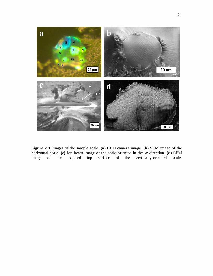
2.9 Images of the sample scale. (a) CCD camera image of the sample scale. (b) SEM

image of the sample scale. (c) Ion beam image of the sample scale oriented in the

xz-direction. (d) SEM image of the exposed top surface of the sample

scale………………………....................................................................................21

2.10 SEM image of the horizontal scale’s top surface after FIB milling……………..22

ix

2.11 SEM image of the melted internal structure when an ion beam current > 430 pA

was used…………………………………………………………………….........22

2.12 SEM image of a single domain…………………………………………………..23

2.13 Cross-sectional scanning electron microscopy images of the individual domains

on the sample scale………………………………………………………………24

2.14 Photonic band diagram of the weevil E. chevrolati……………………………...26

2.15 SEM images of individual single-crystalline domains oriented in Γ-L, Γ-K and Γ-

W directions, with corresponding calculated dielectric function (insets in the

figure)………………………………………………………………………….....27

3.1 The color models: RGB (Additive) and CMYK (Subtractive)………………......33

3.2 Color-matching functions of 1931 CIE standard 2⁰ observer. Red, green and blue

curves represent �̅�, �̅� and 𝑧̅, respectively………………………………………...36

3.3 CIE 1931 xyY color space………………………………………………………..37

3.4 The CIE color space chromaticity diagram……………………………………...39

3.5 xy-chromaticity diagram for multicolored domains……………………………...41

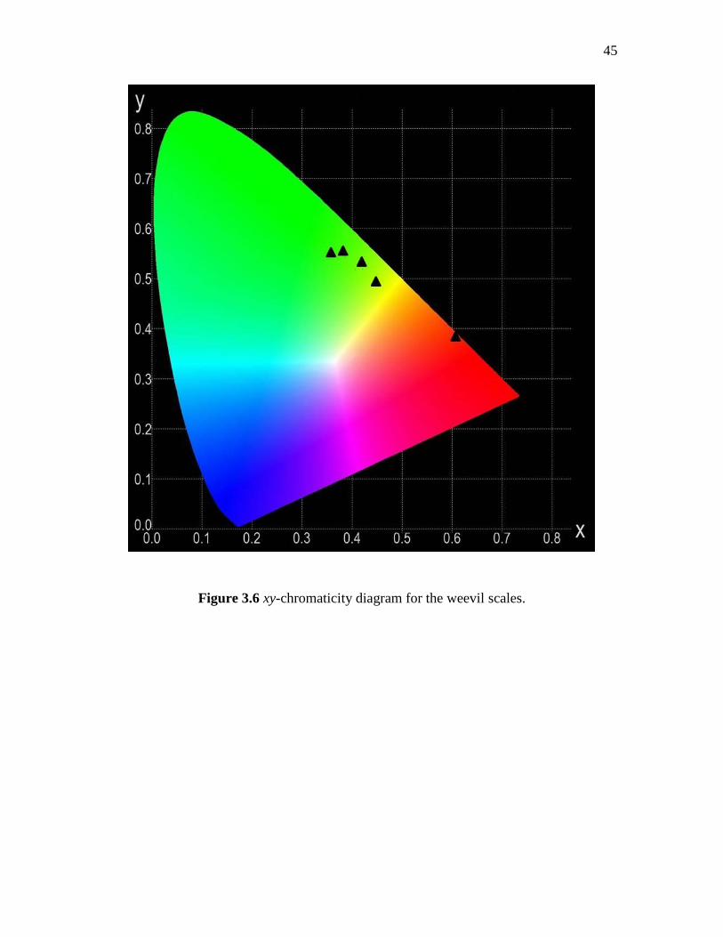
3.6 xy-chromaticity diagram for the weevil scales…………………………………...45

3.7 xy-chromaticity diagram for the whole weevil…………………………………..46

ACKNOWLEDGEMENTS

I express my eternal gratitude and heartfelt thanks to my advisor, Dr. Michael H.

Bartl, for his constant guidance, unconditional support and patience throughout that made

my stint a great learning experience. Dr. Bartl espouses high standards of research and I

am very grateful for his scientific advice and insightful discussions and suggestions and

the wonderful opportunity he gave me to contribute to this interesting and exciting

project. I have greatly benefitted by his intelligence and vast knowledge. I truly

appreciate having him as my advisor.

I extend my sincere gratitude to the members of my supervisory committee, Prof.

Mikhail E. Raikh and Dr. Shanti Deemyad. I am thankful to Prof. Raikh for providing me

with the significant theoretical knowledge through his extremely organized and scholarly

lectures that I could apply in my research work. I am very thankful for and appreciative

of the continued support, guidance and helpful career direction provided by Dr.

Deemyad.

I acknowledge the significant contributions of Dr. Randy Polson in carrying out

the focused-ion beam milling experiments on the beetle scales and Ms. Danielle

Montanari for her band structure calculations and crystal lattice modeling.

I am thankful for the helpful suggestions and feedback I received from all the

members of the Bartl Group, The Bartl Buddies (as we call it!). A special thanks to Dr.

Aditi Risbud for her guidance and words of encouragement.

xi

Lastly, I would like to thank my family for their endless love, care and constant

support.

CHAPTER 1

INTRODUCTION

1.1 Photonic Crystals: Properties and Applications

Researchers have been inspired and determined to explore and solve the mystery

behind the brilliant displays of color and chromatic effects found in the animal and plant

kingdom.1, 2

Though many of the observed colors are due to the pigmentation, several

insects, birds and marine animals have evolved to produce specific types of structures in

their exoskeleton, feathers and bodies for the purpose of coloration.3-9

These structural

colors are produced by diffraction, specular reflection, and interference of light rather

than absorption and diffuse reflection.8, 10-12

The key to structural colors is a periodic

arrangement of dielectric compounds with a periodicity on the order of the wavelength of

visible light.7 Depending upon the periodicity, or lattice parameters, of the structure,

certain wavelengths are classically forbidden to propagate in certain directions through

the structures; hence, they are diffracted and reflected, giving rise to the myriad of

brilliant colors we observe in many insects.

For example, the bright, gem-like reflecting exoskeleton of many species of

beetles, especially Coleoptera and Curculionidae, is not a result of the presence of

pigments but the presence of three-dimensional photonic structures, also referred to as

photonic crystals. To list two particularly interesting beetles, the scales of

Pachyrrhynchus congestus13

weevils have a hexagonal close-packed arrangement of air-

2

spheres built into their exoskeleton, while the weevil Lamprocyphus augustus14

produces

its spectacular green coloration with a diamond-based air-cuticle lattice (i.e., face-

centered cubic system).

In biological systems structural colors are used as a defense mechanism, mating

signals, mimicry or as a camouflage tool to blend into their habitat. Many harmless

organisms have evolved to mimic aposematic* species, for example, the black and yellow

pattern on the hornet moth, Aegeria apiformis, contributes to its resemblance to a wasp or

bee, but is not capable of stinging.15

Animals such as the poison dart frog16

native to

Central and South America and cinnabar moth caterpillar17

display aposematic patterns to

prevent attack by warning potential predators. Not only animals but some plant species

such as scarlet trumpet use their unique pigments also to attract pollinators.18

Millions of years after biology started to develop photonic structures and use

structural colors, modern day research has embraced similar ideas to control light. While

the motivation in biology and technology for developing photonic structures differs (the

former uses these structures to create color effects for camouflage, mimicking, and

signaling, whereas technological applications include coherent control of light,

amplification, and guiding), structural features employed in both biology and technology

are very similar.

In the late 1980s, the quest to find new ways to control light in materials led to the

discovery of photonic band structure materials, also known as photonic crystals. In a

photonic crystal (Figure 1.1), the periodic variation of dielectric constant leads to the

appearance of the photonic band structures. These control how photons move thorough

*Aposematism, a primary defense mechanism, is the use of bright conspicuous coloration or other

perceivable characteristics by the prey animal to warn potential predators.

3

Figure 1.1 Schematics of photonic crystals. Different colors represent different

dielectric materials19

.

the crystal, in a similar way as the periodic arrangement of ions on a lattice gives rise to

the electronic bands which controls the motion of charge carriers in semiconductors.20

Photons propagate through the structure depending on their wavelength. The group of

allowed modes, the wavelengths of light that are allowed to propagate, forms bands. In

several recent studies, several dielectric structures have been predicted (and some also

experimentally confirmed) to show a photonic band-gap, a range of frequencies for which

no electromagnetic modes are classically allowed to propagate through the material.21, 22

Such photonic crystals exhibit a variety of distinct optical phenomena such as

suppression of spontaneous emission20

, omnidirectional mirrors, low-loss waveguiding

and quantum information processing.23

More recent studies show that the position of a

photonic band-gap can be controlled by modifying the refractive index or the periodicity

of the photonic crystal structure.24

4

1.2 History of Photonic Crystals

In 1887, Lord Rayleigh studied the electromagnetic wave propagation in periodic

media and predicted that there exists a one-dimensional photonic band-gap in one-

dimensional photonic crystals.25

These photonic crystals were studied in the form of

periodically arranged multilayer dielectric slabs. About 100 years later, in 1987, two

physicists Eli Yablonovitch and Sajeev John studied photonic crystals independently and

published two milestone papers on high dimensional photonic crystals.20, 26

Yablonovitch,

an American physicist, engineered the photonic density of states, in order to control the

spontaneous emission of materials embedded within the photonic crystal, while John used

photonic crystals to affect the localization and control of light. They created a three-

dimensional structure that exhibited a complete photonic band-gap.21

In 1996, Thomas

Krauss fabricated a two-dimensional photonic crystal structure with photonic band-gaps

at low wavelengths (in the range 800-900nm).27

This led to the novel phenomena in

quantum optics and various technological applications. At the commercial level, photonic

crystals have an excellent application in the form of photonic crystal fibers, developed by

Philip St. J. Russell in 1998.28

1.3 Theoretical Background in Photonic Crystals

Photonic crystals are periodic dielectric structures with zero propagation of

electromagnetic modes for the range of frequencies spanned by the band-gap.20,26

Whenever electromagnetic radiation with a wavelength comparable to the lattice constant

of the photonic crystal is incident upon the crystal, the electromagnetic waves are Bragg-

scattered and undergo constructive or destructive interference. Thus, given the Bragg

condition is satisfied, there exists a range of photon frequencies where no photons are

5

allowed to transmit through the material, called a photonic band-gap. A Brillouin zone

exhibits all the wavevectors k, which are Bragg-reflected by the crystal. Since the

dispersion relation ω(k) is a periodic function of k outside the Brillouin zone, the

calculations for the photonic band-gap are restricted only to the wavevectors k lying

inside the irreducible Brillouin zone instead of considering all possible propagating

directions in the photonic crystal. Hence, all the dispersion curves ω(k) of the photonic

crystal can be represented by the wave vectors k present inside the irreducible Brillouin

zone, which depends on the geometry of the lattice.

In 1928, in his doctoral thesis, Felix Bloch studied the propagation of electronic

waves in three-dimensionally periodic media extending the Floquet’s theorem in one

dimension by Gaston Floquet (1883).29

Bloch proved that waves in a periodic medium

can propagate without getting scattered. He defined the Bloch wave function for a

particle in a periodic environment by a periodic envelope function multiplied by a plane

wave and predicted that the scattering of electrons in a conductor is due to the lattice

defects and not from the periodic atoms.

In 1997, three physicists at the Massachusetts Institute of Technology, John D.

Joannopoulos, Pierre R. Villeneuve and Shanhui Fan applied the same technique to

electromagnetic waves. They showed that one can obtain an eigenvalue equation in only

the magnetic field H by solving Maxwell’s equations as an eigenvalue problem

(analogous to the Schrӧdinger’s equation) starting from the source-free (ρ = J = 0)

Faraday’s and Ampere’s laws at a fixed frequency30

(time dependence 𝑒−𝑖𝜔𝑡):

𝛁 ×1

ɛ(𝐫)𝛁 × 𝐇 = (

𝜔

𝑐)

2

𝐇 (1.1)

6

where 𝛁 ×1

ɛ(𝐫)𝛁 × is the Hermitian eigen-operator, (

𝜔

𝑐)

2

is the eigenvalue, c is the speed

of light, and ɛ(r) , r = (x, y, z), is the dielectric function. The periodic dielectric function

corresponding to a photonic crystal is given by ɛ(r) = ɛ(r + Ri), where Ri are the primitive

lattice vectors (i = 1, 2, 3 for a crystal periodic in one, two, or three dimensions,

respectively).

According to the Bloch-Floquet theorem for periodic eigenproblems, the solutions

to Eq. (1.1) can be chosen in the form 𝐇(𝐫) = 𝒆𝑖𝒌𝐫𝐇𝑛,𝒌(𝐫) with eigenvalues ωn(k)

representing the frequencies of allowed harmonic modes, where k is a Bloch wave

function and 𝐇𝑛,𝒌 is a periodic function satisfying the following equation30

:

(𝛁 + 𝑖𝒌) ×1

ɛ(𝐫)(𝛁 + 𝑖𝒌) × 𝐇𝑛,𝒌 = (

𝜔𝑛(𝒌)

𝑐)

2

𝐇𝑛,𝒌 (1.2)

This equation (1.2) produces a different Hermitian eigenproblem over the primitive cell

of the lattice at each Bloch wavevector k.

If the structure is periodic in all directions, this leads to discrete eigenvalues ωn(k)

which are continuous functions of k with n = 1, 2, ···. The band structure or dispersion

diagram can be obtained plotting these eigenvalues ωn(k) versus the Bloch wavevector k;

where both ω and k are conserved quantities. The eigensolutions are periodic functions of

the wavevector k. By solving equation (1.1) for the first few eigenvalues over the

principle directions in the photonic crystal, the allowed frequencies within the crystal can

be evaluated and summarized in a photonic band diagram.

A complete photonic band-gap can be defined as the range of frequencies ω for

which there are no propagating solutions of Maxwell’s equations (1.2) for any k, with

propagating states above and below the band-gap. The maxima and the minima of the

7

function ω(k) occur at the irreducible Brillouin zone edges, which are obtained by

eliminating the redundant regions inside the first Brillouin zone using the reflection

symmetries.

The harmonic modes can be found by using the variational principle. The

eigenvalues minimize a variational problem in terms of the periodic electric field

envelope 𝑬𝑛,𝒌:

𝜔2𝑛,𝒌 = min𝐄𝑛,𝒌

∫|(∇×𝑖𝒌)×𝐄𝑛,𝒌|2

∫ ɛ|𝐄𝑛,𝒌|2 𝑐2 (1.3)

where the numerator and the denominator correspond to the kinetic and the potential

energy, respectively. By symmetry, the harmonic modes of the propagating

electromagnetic field can be divided into two polarizations, transverse-magnetic (TM)

and transverse-electric (TE), each with its own photonic band structure (dispersion

diagram).

The higher bands are constrained to be orthogonal to the lower bands for 𝑚 < 𝑛.

∫ 𝐇𝑚,𝒌∗ 𝐇𝑛,𝒌 = ∫ ɛ𝐄𝑚,𝒌

∗ 𝐄𝑛,𝒌 = 0 (1.4)

At each k, there exists a gap between the lower dielectric bands concentrated in the high

dielectric region and the upper air bands that are concentrated in the low dielectric. The

dielectric/air bands in the photonic crystal are similar to the valence/conduction bands in

a semiconductor. In order for a complete band-gap to arise in two or three dimensions,

the band gap corresponding to each k point should overlap, which implies a minimum ɛ

contrast.

The existence of a photonic band-gap depends on the two polarizations (TM and

8

TE) of the electromagnetic radiation (classically referred to as the s and p polarizations,

respectively), and the boundary conditions at the material interface.31

An omnidirectional

band-gap is achieved only with a three-dimensional photonic crystal when the incident

electromagnetic radiation with a frequency in the photonic gap region is reflected from

the crystal for all angles of incidence and all polarizations.31

A three-dimensional

photonic structure is a face-centered cubic (fcc) lattice of air cylinders in a high-dielectric

matrix. The first Brillouin zone of such a crystal is a truncated octahedron with an

irreducible Brillouin zone defined by vertices Γ, L, U, X, W and K with origin at the

point Γ = (0, 0, 0), as shown in Figure 1.2. The dispersion curves of the photonic band

diagram can be analyzed by considering the wave vectors k, originating from the Γ-point,

which describe the edge of the polyhedron-shaped irreducible Brillouin zone.

The existence of a complete band-gap depends on the ratio of the dielectric

constants, the volume fraction of the dielectric material, and the geometry of the three-

dimensional periodic structure.32

9

Figure 1.2 Brillouin zones of a face-centered cubic crystal: Truncated octahedron is the

first Brillouin zone, and the polyhedron with vertices Γ, L, U, X, W and K is the

irreducible Brillouin zone.

CHAPTER 2

BIOLOGICAL PHOTONIC CRYSTALS

2.1 Introduction

A delicate interplay of incident light with the intricate patterns of the weevil

Eupholus chevrolati’s exoskeleton scales produces a large number of sparkling colors

and vivid hues. The reason for this beetle’s coloration lies in a hierarchical photonic

structure system covering its exoskeleton, consisting of multicolored micron-sized

domains of three-dimensional photonic crystals. A striking feature of E. chevrolati’s

appearance is that while it has a macroscopic uniform yellowish-green coloration, this

‘uniform’ color is the result of multicolored (from blue to green, yellow and red)

micrometer-sized domains. Figure 2.1 shows various scales with differently colored

domains. To unravel the mystery behind this optical effect, the photonic structure within

each micrometer scale and sub-micrometer domain was investigated using the valuable

characterization techniques such as optical microscopy, scanning electron microscopy

and focused ion beam microscopy. We modeled the three-dimensional architecture of the

photonic crystals from the SEM images, studied the origin and properties of the resulting

photonic band structure, computed the photonic band diagram using MIT’s photonic

bands (MPB) software package,33

and compared the calculations to experimental high-

resolution optical spectroscopy studies.

11

Figure 2.1 Optical microscopy images of iridescent scales of the weevil E. chevrolati,

demonstrating differently colored domains.

2.2 Materials and Characterization

In this section we introduce the experimental techniques used in this thesis

including the optical and structural characterization of biological photonic structures, and

calculation of photonic band diagrams for the structure present inside the exoskeleton of

the weevil E. chevrolati.

2.2.1 Optical Characterization

One of the most common methods to experimentally characterize a photonic

crystal is optical reflectance measurement. The range of wavelengths of electromagnetic

waves, which are forbidden to propagate in a certain direction through the photonic

crystal, are totally reflected, determining the photonic stop-gap (a directional band-

gap).20,26

Experimentally, this is characterized by the presence of an inhibited

12

transmission with an associated reflection peak at the characteristic

frequency/wavelength range.20

The yellowish-green iridescence of the scales found on the exoskeleton of the

weevil E. chevrolati was investigated by the optical microscopy technique. The optical

spectra were taken at normal incidence with an Ocean Optics USB4000 spectrometer

fiber coupled to a Nikon EclipseME600 microscope. White light from a ThorLabs OSL1

Fiber Illuminator was focused onto the specimen using a 20 × objective lens with

numerical aperture (NA) of 0.46. The experimental setup is shown in Figure 2.2. The

reflection measurement was normalized to a high reflectance broadband mirror as 100%.

A pinhole with 0.5 mm aperture was inserted into the image plane of the optical path to

isolate small areas of the exoskeleton (as small as ~5 µm in diameter). The exoskeleton of

the weevil was cut into small sections (~ 1 mm), and reflectance spectra from the

individual domains in the scales were measured and analyzed.

Figure 2.2 Experimental set up for optical characterization.

13

2.2.2 Structural Characterization

The photonic structure inside of iridescent scales of the weevil E. chevrolati was

examined by high-resolution structural analysis based on scanning electron microscopy

(SEM) combined with focused ion beam (FIB) milling. SEM and FIB were conducted

using a FEI NanoNova 630 microscope and a FEI Helios NanoLab 650 system,

respectively. The structural characterization of the weevil scales was executed by first

gently scraping a few scales from the exoskeleton of the weevil onto a microscope slide

using a razor blade. The scales were then transferred onto the conductive carbon adhesive

tab SEM sample holder. The scale was carefully oriented vertical using a scalpel. By

orienting the scale vertical and adjusting the angles of rotation and tilt of the FIB stage, a

layer of thickness ~0.7 µm was removed from the top surface of the scale using FIB with

ion beam current of 430 pA and 30 kV accelerating voltage. The subsurface internal

photonic structure thus exposed, provided us with a view of the all domains within a

single scale. High resolution images of the structure of each domain were taken by FEI

NanoNova SEM. Since the nonconductive specimens tend to charge when scanned by the

electron beam using high vacuum mode, an ultrathin layer of gold was deposited on the

top surface of the scale by sputter coating before SEM imaging.

The SEM images were later processed using the image-processing software

ImageJ. The structural parameters were obtained from analyzing the structural features of

the cross-sectional SEM images of each domain. Using the quantitative information thus

obtained, a face-centered cubic lattice-based30

three-dimensional photonic structure of the

domains was created. The two-dimensional cross-sectional projections of the structure

model obtained by making oblique cuts through the volume were compared with the

14

SEM images taken of each domain on the weevil scale.

2.3 Results and Discussion

In this section we present our detailed analysis of the observed wide range of

chromatic effects in the weevil E. chevrolati (dried specimen) from spectral reflection

studies and anatomy of the weevil by implementation of high-resolution imaging

techniques.

2.3.1. Micropixelation and Color Mixing

To understand the origin of the angle-independent homogeneous yellowish-green

color in the studied weevil (see Figure 2.3 (a)), we employed the routinely used

characterization technique, optical reflection spectroscopy.

A typical optical reflectance spectrum of large sections of the weevil (100’s of

scales) is given in Figure 2.4. It displays a broad reflection peak centered at ~540 nm

consistent with the weevil’s macroscopic yellowish-green appearance. The large number

of spectral features of the reflection peak indicates that this reflection spectrum is a

mixture of many individual reflection peaks originated from different scales. To test this

hypothesis we collected reflectance spectra from individual scales of the weevil’s

exoskeleton. These measurements revealed that reflection properties differ strongly from

scale to scale. This finding is summarized in Figure 2.5, which compares the envelope

reflection peak of a large area of the weevil’s surface with the wavelength position of the

peak maxima of 17 individual scales. It is evident that the overall reflectance behavior of

this weevil is the result of color mixing at the micrometer-scale.

Moreover, analysis of the optical reflection micrographs of individual scales

15

Figure 2.3 Multiple levels of the weevil E. chevrolati’s hierarchical structure:

exoskeleton, scales and domains. (a) Photograph of the weevil E. chevrolati. (b) Optical

microscopy image of iridescent scales attached to the exoskeleton of E. chevrolati under

white light illumination. (c) Magnified optical microscopy image of individual scales

showing differently-colored domains.

16

450 500 550 600 650 700

0

5

10

15

20

Refl

ecta

nce (

%)

Wavelength (nm)

Figure 2.4 Optical reflectance spectrum for the weevil E. chevrolati.

450 500 550 600 650 700

0.0

0.2

0.4

0.6

0.8

1.0

450 500 550 600 650 700

0.0

0.2

0.4

0.6

0.8

1.0

Wavelength (nm)

Ref

lect

an

ce (

norm

ali

zed

)

Figure 2.5 Reflectance spectra for E. chevrolati as an envelope to the peak reflection

from individual scales.

17

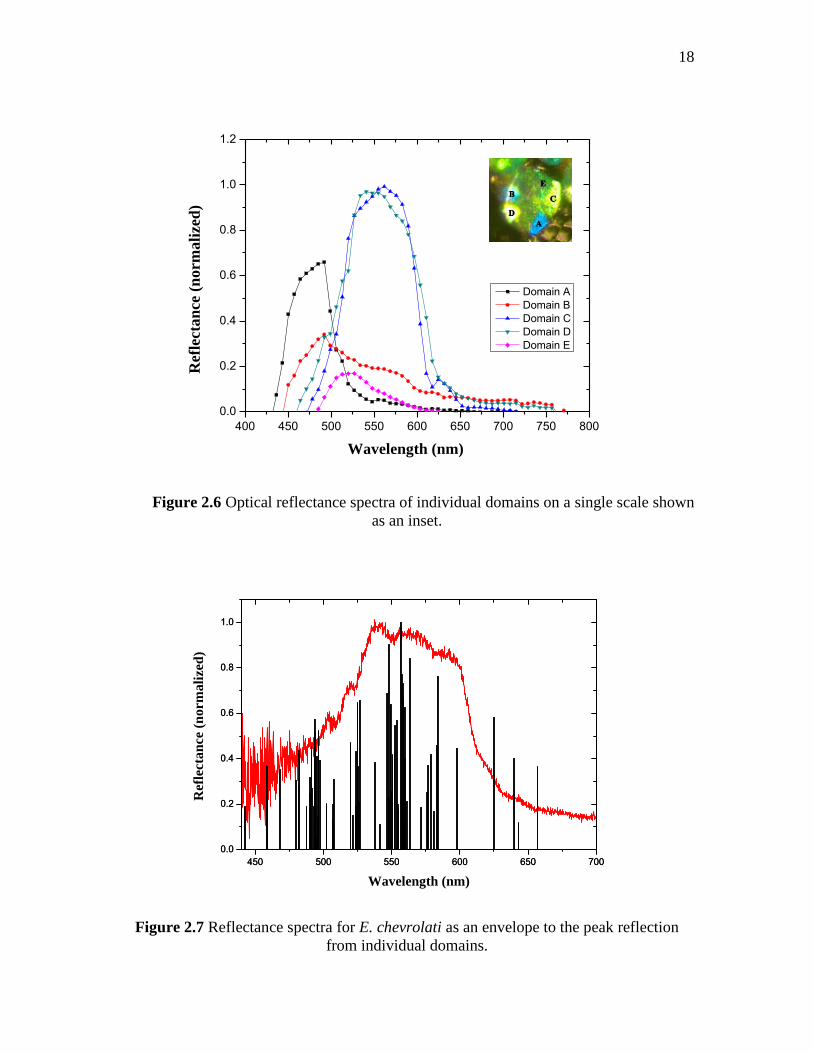
(Figure 2.1) shows that color-mixing occurs at even smaller length scales, namely

between individual domains within a single scale. We therefore optimized our micro-

reflectance spectroscopy set-up to allow us to measure spectra of individual scale

domains (around 2-10 µm in size). The resulting spectra of five domains of a particular

scale are presented in Figure 2.6 (together with the optical micrograph) and demonstrate

the distinct reflection properties of individual domains.

These high spatial-resolution measurements were repeated for a total of 80

different domains within different scales from multiple areas of the weevil’s exoskeleton.

The results are summarized in Figure 2.7. A comparison of all the peak maxima

wavelength positions with the envelope spectrum demonstrates excellent agreement,

confirming the hypothesis of additive color-mixing of pixel-like domains as the origin

behind the yellowish-green coloration of the weevil E. chevrolati. In addition, the

generated mixed color depends on the luminance levels of all individual pixelated color

domains. A full range of colors perceivable by a human observer can be produced from

the colored domains and an adjustment of their luminance levels. To further analyze this

color-mixing phenomenon and find an explanation for the weevil’s angle-independent

coloration with a dull, low saturated hue, the concept of color theory has been applied

and will be discussed in detail in Section 3.2 of Chapter 3.

2.3.2 SEM Structural Studies of Individual Scales and Domains

To examine the origin of the different coloration of individual domains the

structural properties of scales and domains were investigated by a combined SEM

imaging and FIB milling study. For this, the exoskeleton of a dead, dried weevil

specimen was dissected into small pieces and individual scales, and mounted onto SEM

18

400 450 500 550 600 650 700 750 800

0.0

0.2

0.4

0.6

0.8

1.0

1.2

Ref

lecta

nce (

no

rm

ali

zed

)

Wavelength (nm)

Domain A

Domain B

Domain C

Domain D

Domain E

Figure 2.6 Optical reflectance spectra of individual domains on a single scale shown

as an inset.

450 500 550 600 650 700

0.0

0.2

0.4

0.6

0.8

1.0

Refl

ecta

nce (

norm

ali

zed

)

450 500 550 600 650 700

0.0

0.2

0.4

0.6

0.8

1.0

Wavelength (nm)

Figure 2.7 Reflectance spectra for E. chevrolati as an envelope to the peak reflection

from individual domains.

19

sample holders. The FIB milling technique was then used to cut scales and expose the

interior cuticle structure. An example of a random cross-sectional cut is presented in

Figure 2.8.

In a single scale, differently-colored domains are horizontally stacked and spread

across its entire volume, and the structure of each domain extends from the top to the

bottom surface (~5 µm) of the scale. To investigate the structural arrangement of a

domain generating a specific wavelength, the entire scale was first mapped with all the

existing domains on its CCD image (see Figure 2.9 (a)), then, as mentioned in Section

2.2.2, the outermost protective layer of the vertically-oriented scale, as shown in Figure

2.9 (c), was removed from the top using the FIB technique. It was observed that the use

of an ion beam on the horizontal scale on the SEM stub resulted in an uneven top surface,

as can be seen in Figure 2.10. However, after the alignment of the xz-plane of the scale

with the ion beam direction and limiting the ion beam current to 430 pA (higher values of

current rendered the soft chitin structure to melt as can be seen in Figure 2.11) we were

provided with a clean-cut top surface with clearly-defined domain boundaries as shown

in Figure 2.9 (d).

The high-resolution image of the scale’s top surface, thus obtained, was matched

with its CCD image, and each individual domain was depicted in its SEM image (Figure

2.9 (d)). To study the structural characteristics of each domain, individual domains were

then imaged using SEM, as shown in Figure 2.12 and 2.13.

Comparison of the exposed structural features of several different cross-sectional

cuts with previous studies in the Bartl group on other types of weevils (in particular,

Lamprocyphus augustus) revealed strong similarities. More detailed structural

20

Figure 2.8 SEM of the exposed side surface of the sample scale.

examination confirmed a similar structure of ABC stacked layers of air cylinders

arranged in a face-centered-cubic (fcc) lattice in a surrounding dielectric matrix made of

chitin (a polysaccharide-based biopolymer with refractive index of 1.53).

Quantitative analysis yielded a height and radius of the air cylinders of 300 ± 25

nm and 71 ± 7 nm, respectively. The lattice constant, a, was found to vary in the range

between 360 and 400 nm.

21

Figure 2.9 Images of the sample scale. (a) CCD camera image. (b) SEM image of the

horizontal scale. (c) Ion beam image of the scale oriented in the xz-direction. (d) SEM

image of the exposed top surface of the vertically-oriented scale.

22

Figure 2.10 SEM image of the horizontal scale’s top surface after FIB milling.

Figure 2.11 SEM image of the melted internal structure when an ion beam current > 430

pA was used.

23

Figure 2.12 SEM image of a single domain.

24

Figure 2.13 Cross-sectional scanning electron microscopy images of the individual

domains on the sample scale.

25

2.3.3. Band Structure Studies and Comparison to Optical Properties

Due to the presence of additional symmetries of the face-centered cubic lattice

structure, the energy bands are invariant under spatial reflection symmetry, the

wavevectors describing an irreducible Brillouin zone of the lattice are sufficient to define

the photonic band structure. The maxima and minima of the eigenvalues occur at the

edges of irreducible Brillouin zone defined by the vertices Γ, L, U, X, W and K. The

photonic stop-bands are the gaps between any two consecutive allowed modes in the

photonic band diagram. As described in Section 1.3 of Chapter 1, electromagnetic modes

inside a photonic crystal structure can be calculated by finding the eigenvalues of the

modified Hermitian eigenproblem (the frequencies of allowed harmonic modes). MIT’s

photonic bands (MPB) software, designed for the study of photonic band-gap materials,

computes the definite-frequency harmonic modes of Maxwell’s equations in periodic

dielectric structures and dispersion relations.33

Figure 2.14 presents a photonic band

diagram of the weevil E. chevrolati’s photonic crystal structure with a face-centered

cubic arranged air-cylinder lattice, calculated using the above mentioned photonic bands

software.†

A three-dimensional model of the photonic structure inside the weevil was

constructed using the evaluated structural parameters. Two-dimensional projections were

obtained by making cuts along specific directions through the constructed volume of with

face-centered cubic air-cylinder lattice structure (Figure 2.15).† These model crystal faces

were compared to SEM images of the top-surface domains of individual scales (see

Figure 2.13). A detailed comparison is shown in Figure 2.15, where the calculated

† The three-dimensional modeling and photonic band structure calculations (using the MIT photonic bands

(MPB) software) were performed by Danielle Montanari, a graduate student in the Bartl group.

26

0.0

0.2

0.4

0.6

0.8

1.0

1.2

1.4

Fre

qu

ency

(c/

a)

Bloch wavevector

L X U W

Figure 2.14 Photonic band diagram of the weevil E. Chevrolati.

27

Figure 2.15 SEM images of individual single-crystalline domains oriented in Γ-L, Γ-K and Γ-W

directions, with corresponding calculated dielectric function (insets in the figure).

28

dielectric function of model crystal faces in the directions Γ-L, Γ-K and Γ-W is

superimposed over the SEM images of individual domains. It was found that the domains

within the weevil scales do not follow specific main orientation. Each domain, based on a

face-centered cubic lattice, within a scale is relatively oriented in a different direction

resulting in only a certain range of wavelengths in the electromagnetic spectrum being

reflected by it.

From the calculated frequency stop-band positions along main lattice directions,

the corresponding wavelength ranges can be calculated from the mid-gap frequency

values ωo, by choosing structurally-relevant lattice constants. For the weevil photonic

crystal structure, we determined the lattice constant to be in the range 360-400 nm. Thus,

we calculated wavelength stop-gap positions for all main lattice directions for lattice

constants of 360, 380 and 400 nm. Results are listed in Table 2.1. The architecture of the

weevil E. chevrolati’s exoskeleton consists of numerous scales, each scale with several

domains and each domain built on the same set of building blocks, fcc cubic lattice

structure, but different dimensions, more specifically, lattice constants. Depending on

which facet of the domain’s lattice structure is oriented in the direction of incident light,

the structure forbids a range of wavelengths to propagate through the structure.

It can be concluded from the calculated values that each domain within the scale

of the weevil E. chevrolati is capable of exhibiting a wide wavelength range within the

visible part of the electromagnetic spectrum, with different directions spanning different

ranges of wavelengths. As discussed earlier in Section 2.3.1, the yellowish-green

coloration of the weevil results from the additive mixing of different colors reflected

from different domains.

29

Table 2.1 Ranges of wavelength reflected by the photonic crystal structure with different

lattice constants.

Directions Mid-gap Frequency, ωo

(in units of c/a) Wavelength Range (nm)

a = 360 nm a = 380 nm a = 400 nm

Γ-L 0.66 511-585 540-618 568-650

Γ-X 0.74 476-493 503-521 529-548

Γ-U 0.78 451-474 476-500 501-526

Γ-W 0.80 441-462 465-487 490-513

Γ-K 0.79 444-470 469-496 494-522

The comparison of structural data, optical results and band structure calculations

suggest that the wavelength ranges exhibited by the weevil were generated from the same

crystal lattice structure but from differently oriented domains within a lattice constant

range of 360-400 nm. For example, only the fcc lattice structure with lattice constant of

400 nm spans the red wavelength region in the Γ-L direction, whereas the green and blue

wavelengths generate from at least one of the directions of the lattice built with a lattice

constant ranging between 360 and 400 nm.

CHAPTER 3

MATHEMATICAL REPRESENTATION OF COLORS ON A

COLOR SPACE

3.1 Introduction

As with all living organisms, animals evolve through thousands of generations,

which has an enormous impact on their appearance and behavior. This process of change

often results in accordance with their surroundings and the changes in their survival plan.

Theories of evolution explain how various species are considered related to one another,

like humans and apes, for example.

Colors existed long before the conception of life in Mother Nature. However,

studies show that the same objects are perceived of as having different colors by different

observers. Depending on the wavelength ranges in the electromagnetic spectrum required

to reproduce their full visible spectrum, animals can be categorized into dichromats,

trichromats, tetrachromats and pentachromats.34

Humans and some other mammals have

evolved trichromacy from early vertebrates.35-38

It is estimated that trichromatic humans

can discern up to 2.3 million different surface colors39

and can distinguish wavelengths

with a difference of as little as 0.25 nm40

. Fish and birds are tetrachromats, that is, they

have four types of cone cells and can detect energy of ultraviolet wavelength as well,

whereas most other mammals such as the domestic dog and the ferret are dichromats.41

31

Colors help animals in identifying different objects.40, 42

Several ancient scientists including Aristotle were intrigued by the theory of color

and the physical reason behind its existence. Isaac Newton43, 44

, Thomas Young, James

Clerk Maxwell45

and Lord Rayleigh, who are considered the giants in the field of physics,

studied the nature of light and developed theories of color vision. In the early 18th

century, Thomas Young presented his hypothesis on color perception in his lectures,

stating that the presence of three kinds of nerve cells in the human eye results in the

perception of different colors.46

Color vision is the ability to interpret the surrounding environment by processing

the information contained in the visible light.47

The color of an object is a result of the

mixture of all wavelengths in the light leaving the surface of that object. This depends on

the object’s surface properties, its transmission properties and its emission properties.

The viewer’s perception of the color of the object depends on the ambient illumination

and the characteristics of the perceiving eye and brain.

This chapter discusses the wide color ranges produced in the biological world,

and the mathematical representation of perceived colors using color space diagrams. The

color gamut can be specified in a color space such as the CIE XYZ color space, by

calculating the tristimulus values of the three primaries: red, green and blue. The XYZ

color system used here to produce the color gamut was developed by CIE (Commission

Internationale de l'Eclairage) in 1931.48, 49

The perceived color of an object is a visual

effect of a specific color combination, which makes it of absolute importance to

understand the behavior of color mixtures in case of light (additive) and chemical dyes

(subtractive). Color theory provides a guidance to color mixing and perceived colors.

32

3.2 Color Theory

Colorimetry, the science of color, includes the perception of a color by the human

brain and eye50-52

, the physics of electromagnetic radiation visible to the human eye, and

the origin of color in materials.53-55

Colors can be broadly categorized in three ways: primary color, secondary color

and tertiary color. Primary color cannot be produced from any combination of other

colors, whereas secondary and tertiary colors can be created from a combination of two

(primary) colors and three (primary or secondary) colors, respectively. Colors can be

mixed together to produce other colors. This mixing of colors can be additive or

subtractive.56

The creation of color by mixing light of different colors is known as

additive color synthesis. The light sensitive cones in the human eye detect these light

signals and send them to the brain for processing this information. This biological process

is explained in detail in the following section. The additive color process is observed in

television screens where an image is generated by mixing small pixels of red, green and

blue lights. The subtractive color synthesis is the creation of color by mixing different

colors of dyes or paints. The RGB color model is an additive color model, whereas

CMYK color model57

is a subtractive color model (see Figure 3.1).

The concept of color can be divided into two parts: chromaticity and brightness.

The chromaticity represents the quality of a color, and consists of two independent

parameters, hue and saturation. Brightness is one of the three psychological dimensions

of color perception which refers to the visual stimuli of the light intensity. Hue refers to

the purity of a color, and is defined as the degree to which the stimulus can be related

similar to the unique hues (red, green, yellow, and blue). Saturation represents the degree

33

Figure 3.1 The color models: RGB (Additive) and CMYK (Subtractive).

by which a color differs from the gray of the same brightness.

An average human observer’s response to a color can be described in terms of the

amount of three primary colors (red, green, and blue) mixed together additively or

subtractively to produce each wavelength of the visible range before it is perceived by the

human eye.58

3.3 The Human Eye and Color Mixing

Human visual perception is based on the color and the distance59

. Due to the

spatial contrast sensitivity function of the human eye, the closer it is to an object, the finer

detail it can resolve. At greater distances, the human eye tends to lose its visual acuity,

which is a measure of angular resolution, specified in units of cycles per degree (CPD).

The maximum resolution is 50 CPD for a human eye with excellent visual acuity.60

The

farther the eye moves away from an object (from the microscopic to the macroscopic

view), the less resolved the features of the object become. This leads to the merging of

34

colors as the human brain tries to process the incoming information. Instead of seeing

resolved spots/features, the human eye sees a total image of the object. In order to

understand the response of a human observer to the colors found in their surroundings, it

is of importance to understand the biological model of the human eye.

A human retina is a mosaic of two basic types of light sensors, also called

photoreceptors: cone cells and rod cells, which are responsible for color and peripheral

vision, respectively.61

Each cell supplies information required by the visual system to

create awareness of the surrounding environment through physical sensation. The

resulting perception is known as eyesight or vision. Visual acuity, a property of the cone

cells which are highly concentrated near the center of the retina called fovea centralis, is

the ability to distinguish fine detail.62

The lens of the human eye focusses the incoming

light onto the photoreceptive cells of the retina, which is a part of the brain. The retinal

neurons detect visible electromagnetic radiation and respond by producing neural

impulses. Specifically, the photoreceptor proteins in the cells absorb the photons resulting

in a change in the cell’s membrane potential and produce electrical signals, which are

processed by the brain to create an image of the visible surrounding environment. The

color is detected by the cone cells which function best in the bright light. Although the

rod cells are extremely sensitive to dim light, they cannot resolve sharp images or color.

This explains why colors cannot be seen at night as only one photoreceptor cell is active.

Humans are trichromats.47, 61, 63

Their retina consists of three different types of color

receptors (called cone cells in vertebrates) with different absorption ranges of the

electromagnetic spectrum, each containing a different photopigment. Young’s idea of

color vision was that it is a result of the three photoreceptors.46

This was later expanded

35

by Helmholtz using color-matching experiments.64

Each of the three types of cone cells

in the human retina contains a different type of photosensitive pigment.65

Each

photopigment produces a neural response only when it is hit by a photon with a specific

wavelength of light. The response curve is a function of wavelength and varies for each

type of cone, giving the perception of any color sensation. The spectral sensitivity peaks

of the three cone cells S, M, and L lie in the wavelength ranges 420-440 nm (S, short

wavelength), 530-540 nm (M, medium wavelength) and 560-580 nm (L, long

wavelength). They give three different signals based on the extent to which each cone

cell is stimulated. These values of stimulations are called tristimulus values. The set of all

possible tristimulus values determine the color space for a human observer.

3.4 Calculation of Chromaticity Coordinates

The tristimulus values depend on the observer’s field of view due to the

distribution of cone cells in the human eye, so CIE defined a standard observer, which

represents the chromatic response of a human within a 2⁰ arc of the fovea centralis‡.66, 67

This particular angle was chosen by CIE because the fovea, a depression in the inner

retinal surface, contains only the color-sensitive cone cells.61

The chromatic response of

an observer can be represented mathematically by the color-matching functions as shown

in Figure 3.2, which when combined with the spectral power distribution of the incident

light and the spectral reflectance leads to the tristimulus values of a color.

A color can be produced by additively mixing the red, green and blue color

components of visible light. The primary colors are represented as X for red, Y for green

and Z for blue.6 The magnitude of the tristimulus values of a color gives the amount of

‡ A part of the human eye retina, where the density of cone-cells is the highest, responsible for sharp central

vision.

36

400 450 500 550 600 650 700 750

0.0

0.5

1.0

1.5

2.0

Co

lor-m

atc

hin

g f

un

cti

on

s

Wavelength (nm)

Figure 3.2 Color-matching functions of 1931 CIE standard 2⁰ observer.

Red, green and blue curves represent �̅�, �̅� and 𝑧̅, respectively.

each color required to be mixed additively in order to match a particular color. The

chromaticity coordinates x and y can be computed by following the standard procedure

given by CIE.49

The CIE XYZ color space, more specifically, CIE xyY color space is a horseshoe-

shaped three-dimensional representation of all visible colors to a human observer, i.e., the

gamut of all visible chromaticities where the solid outline represents the ‘pure’ hues that

are perceivable to the human eye as shown in Figure 3.3. The parameter Y is a measure of

brightness of a color, and the chromaticity of a color is defined by the parameters x and y.

37

Figure 3.3 CIE 1931 xyY color space.

It is favorable to have a representation of ‘pure’ color in the absence of brightness.68

The

chromaticity coordinates can be conveniently represented using the CIE XYZ model.

Hence, this specific color model was used to define the color gamut, for the biological

photonic structures for a standard human observer.

The color perceived by a human observer can be represented numerically by the

integral of the product of the spectral distribution of light source, spectral reflectance or

transmittance of the object viewed and the color matching function of the standard

observer over the visible range of the electromagnetic spectrum 380-780 nm.69

38

𝑋 = 𝑘 ∫ 𝑅(𝜆)𝐼(𝜆)�̅�(𝜆)

380

780

d𝜆

𝑌 = 𝑘 ∫ 𝑅(𝜆)𝐼(𝜆)�̅�(𝜆)

380

780

d𝜆

𝑍 = 𝑘 ∫ 𝑅(𝜆)𝐼(𝜆)𝑧̅(𝜆)

380

780

d𝜆

where �̅�(𝜆), �̅�(𝜆) and 𝑧̅(𝜆) are the color-matching functions49, 70

, 𝐼(𝜆) is the spectral

power distribution of the light source, R(λ) is the spectral reflectance, dλ is the interval of

wavelength and k is the normalization constant defined as 𝑘 = 100 ∫ 𝐼(𝜆)𝑦 ̅d𝜆⁄ .

The tristimulus values X, Y and Z thus obtained are normalized to obtain the three

chromaticity coordinates x, y and z as below,

𝑥 =𝑋

𝑋 + 𝑌 + 𝑍

𝑦 =𝑌

𝑋 + 𝑌 + 𝑍

𝑧 =𝑍

𝑋 + 𝑌 + 𝑍

Only two chromaticity coordinates, x and y, are needed to define the color of an object

since x + y + z = 1. The two coordinates x and y can be plotted to obtain a two-

dimensional diagram of all possible visible chromaticities called the xy-chromaticity

diagram. The two-dimensional chromaticity diagram demonstrates a linear relation

between the colors when mixed additively as shown in Figure 3.4. A straight line drawn

joining the chromaticity coordinates of any two colors that are mixed includes the

39

Figure 3.4 The CIE color space chromaticity diagram.

chromaticity coordinates of all possible colors of the mixture. In case three colors are

mixed additively, all the colors that can be produced by mixing any fraction of those

three colors lie within the triangular region on the diagram formed by connecting the (x,

y) coordinates of the individual colors. The triangular region, thus formed, is called the

color gamut.6 The color gamut of a device or process is specified in the hue-saturation

plane and is defined as that portion of the color space which can be reproduced. An

unrealized goal within the color display engineering is a device that is able to reproduce

the entire visible color space!

3.5 Results and Discussion

Colorful beetles have been studied by various research groups8, 71-77

and it has

been experimentally shown that the selective reflection of light by multifaceted

40

arrangement of photonic structures inside exoskeleton cuticle scales leads to the brilliant

structural coloration.14, 78

The weevil E. chevrolati belongs to one of the largest animal

family with over 400 species all over the world, called Curculionidae. An average adult

weevil is about 1 - 40 mm long and can be recognized by its elongated head that forms a

snout and antennae with small clubs. These weevils have a somber yellowish-green

appearance, as can be seen in Figure 2.3 (a).

In our research, we chose to study the E. chevrolati weevil because of the brilliant

multicolored micron-sized domains in its scales with three-dimensional photonic crystal

based internal structure. E. chevrolati proved to be an excellent model for:

a. studying the mechanism behind selective angle-independent reflectance

from the structural architecture.

b. understanding its usual dull, pastel-type appearance, in spite of the

presence of bright differently-colored domains on its exoskeleton.

c. producing the color gamut, range of reproducible colors, as observed by a

standard human observer.

The range of colors which can be reproduced by the biological photonic structures was

defined by following the same procedure for the calculation of the chromaticity

coordinates x and y, as explained in Section 3.4. The color gamut for the E. chevrolati

weevil (Figure 3.5) was defined on the CIE 1931 chromaticity diagram by considering

differently-colored domains within its scales, and calculating the xy-chromaticity

coordinates of the three individual domains as listed in Table 3.1. Figure 3.5 shows the

corresponding xy-chromaticity diagram containing the coordinate points of selected

domains of weevil scales.

41

Figure 3.5 xy-chromaticity diagram for multicolored domains.

42

Table 3.1 xy-chromaticity coordinates for the individual domains on the weevil.

Scale No. x y

1 0.59 0.40

2 0.34 0.54

3 0.14 0.19

4 0.44 0.51

5 0.23 0.25

6 0.19 0.21

7 0.16 0.55

8 0.41 0.54

9 0.40 0.50

10 0.15 0.13

11 0.24 0.57

12 0.21 0.44

13 0.27 0.30

14 0.48 0.42

15 0.21 0.25

16 0.24 48

17

18

0.30

0.25

0.54

0.38

43

The area lying within the lines connecting the domain’s chromaticity coordinates

forms the color gamut for the weevil. This area represents all possible colors visible to an

average human observer, which can be produced upon the incidence of light on these

domains on the weevil. In contrast to the three-color RGB gamut in electronic display

systems (TV screens79

, for example), these biological systems demonstrate a wide gamut

of colors which can be reproduced by the additive-mixing of reflected lights from a

number of colored domains spanning almost the entire visible wavelength range.

The calculated chromaticity coordinates corresponding to individual scales on the

weevil are listed in Table 3.2. The corresponding locations in the xy-chromaticity

diagram are shown in Figure 3.6. On comparing the chromaticity diagram for individual

scales (Figure 3.6) with the one obtained for individual domains (Figure 3.5), we found

that all the ‘color’ coordinates of individual scales lie within the color gamut produced

for the three domains of red, green and blue-color. Interestingly, due to the low frequency

of occurrence of blue domains within individual scales, the overall mixed color of

individual scales is located far from the blue range in the xy-chromaticity diagram.

Similarly, when analyzing the color of a whole weevil (without resolving

individual domains or scales), the color gamut is reduced to a single point in the

yellowish-green area on the xy-chromaticity diagram, as shown in Figure 3.7. The

chromaticity coordinates were calculated to be (0.43, 0.55) in excellent agreement to the

observed uniform yellowish-green color of this weevil.

Detailed analysis of the color gamut produced in different size-levels suggested

the additive mixing of primary colors occurring in the E. chevrolati weevils before the

reflected colors are perceived by an observer.

44

Table 3.2 xy-chromaticity coordinates for the individual scales on the weevil E.

chevrolati.

Scale No. x y

1

2

3

0.42

0.38

0.61

0.52

0.55

0.39

4

5

0.44

0.36

0.49

0.54

45

Figure 3.6 xy-chromaticity diagram for the weevil scales.

46

Figure 3.7 xy-chromaticity diagram for the whole weevil.

47

In addition to the color coordinate analysis, the color mixing in E. chevrolati

weevils is further supported by their dull appearance. The weevil appears to be of dull

yellowish-green color when viewed with an unaided eye from a distance but differently

colored brilliant domains become visible when viewed under the microscope. This is a

result of the pointillistic color mixing since the primary-colored domains are placed so

close to one another on the weevil’s exoskeleton that the reflected colors from these

domains merge to generate a perception of other colors.80

Patterns beyond the neural

resolution limit81

are removed from the retinal image by the optical system of the human

eye.82

Pointillism is a painting technique in which the individual bright dots of different

hues are placed so that the color spots blend into a fuller range of tones.83, 84

Most likely,

this macroscopic dull yellowish-green appearance helps the weevil to hide in its

surrounding habitat from its predators such as birds.§85, 86

The mathematical representation of colors (color modeling) and the physical

phenomena taking place inside the human eye suggest that the colors reflected from the

exoskeleton of the studied weevil are mixed additively before the color information is

processed by the human brain. In spite of a wide range of colors produced by the

photonic crystal structure inside the exoskeleton of weevil E. chevrolati, the human eye

perceives only the final color resulting from the additive-mixture of lights of different

colors.

3.6 Conclusions

We studied the weevil E. chevrolati using color theory and xy-chromaticity

diagrams based on the CIE XYZ color model. We found the exoskeleton of the studied

§ A typical bird eye responds to the wavelength range of about 300 - 700 nm in addition to the ultraviolet

wavelength (300 – 400 nm).

48

weevil is studded with micron-sized brilliantly colored domains, arranged beautifully in a

pixel-like alignment similar to that found in modern-day display systems. By carefully

examining the weevil microscopically and by representing the observed colors

mathematically with the help of color models and reflectance spectra measurements, we

found that the perceived yellowish-green color of the weevil is a result of the additive

color mixing of the reflected lights from the photonic structured domains in its scales. As

a possible practical application, this micropixelation and color mixing in the biological

photonic structures, where the individual domains serve as primary color sources, can be

replicated synthetically to be used in the RGB LED lighting designing, which consists of

a red, a green and a blue LED, and delivers a color gamut to screens. Also, the distance

between the red, green and blue points can be increased to reproduce more vivid colors,

much similar to the pointillistic color mixing technique.

CHAPTER 4

SUMMARY AND CONCLUDING REMARKS

We have studied the chromatic effects in biological three-dimensional photonic

crystal structures (iridescent exoskeleton scales of a weevil) operating at visible

wavelengths by a range of experimental and modeling techniques. The optical and

structural properties of the biological photonic crystal were studied by high-resolution

scanning microreflectance spectroscopy, focused ion beam milling and scanning electron

microscopy. From these structural insights the photonic band structure was determined

using MIT’s MPB software that combines Maxwell’s equations with solid-state physics

concepts. In addition, the peculiar pointillistic coloration scheme of the weevil was

investigated using colorimetric**

concepts, and an interesting color-mixing strategy was

discovered.

We found that the structural coloration in the weevil E. chevrolati is a

consequence of the structural arrangement of individual color-producing elements,

referred to as photonic domains, which contain the same photonic crystal lattice structure

but slightly different lattice parameters (varying between 360 and 400 nm) and crystal

orientations. The weevil’s exoskeleton is a multicomponent representation of micron-

sized photonic structures with varying dimensions.

**

Science used to quantify and describe physically the color perception of a human observer.

50

The photonic architecture was investigated by optical and structural techniques.

Our reflectance measurements for the weevil’s hierarchical structure consisted of

multiple levels: domains, scales and exoskeleton. These detailed, hierarchical studies

confirmed the proposed theory of additive color mixing as the reason behind the

yellowish-green coloration of the weevil. We observed that the reflectance spectrum of a

large section of the weevil encloses the peak reflectance maxima positions for the

individual domains and the scales.

On the microscopic level, we investigated the three-dimensional structure of the

photonic crystal within each domain using the high-resolution cutting and imaging

techniques such as focused ion beam milling and scanning electron microscopy. These

studies provided us with the lattice dimensions and existing internal structural

organization and presented the basis for three-dimensional structural modeling and

photonic band structure calculations. Using MIT’s photonics bands software, the

forbidden frequencies ranges for light propagation in the weevil’s photonic crystal

structure were determined. In detail, we first compared the internal photonic structure

(from electron microscopy imaging) with the cross-sectional images of the cuts through

the re-constructed three-dimensional dielectric model (obtained from band structure

calculations) based on face-centered cubic lattice structure along specific directions. We

found good overlap between the two-dimensional model crystal faces with the structural

images, confirming the ABC stacked layers of air cylinders ordered in a fcc-cubic lattice

in a dielectric material.

The calculated photonic band structure of the weevil’s photonic crystal possesses

stop-gaps in all main lattice directions (L-Γ, Γ-X, Γ-U, Γ-W and Γ-K). It was discovered

51

that irrespective of the lattice constant value, longer wavelengths (reds) were generated

only from the Γ-L direction, whereas the shorter ones (violets) were forbidden to enter

the crystal in the Γ-W and Γ-K directions. We observed that the maximum range of colors

that can be produced by a particular domain depends on the value of lattice constant. We

found that photonic structures inside the exoskeleton of the weevil based on different

lattice constants of 360 nm, 380 nm and 400 nm yield overall wavelength ranges between

441 – 585 nm, 465 – 618 nm and 490 – 650 nm, respectively (as listed in Table 2.1). This

result suggests that the sophisticated microdomain orientation of the fcc-based photonic

structures of the weevil E. chevrolati generates a minimum wavelength of ~441 nm

(violet region of electromagnetic spectrum) and a maximum of ~650 nm (the red region).

This is in excellent agreement with our optical reflectance spectroscopy results for

individual domains, with a minimum observed wavelength of ~442 nm and a maximum

of ~657 nm (see Figure 2.7).

As a major contribution of this thesis, we tested our hypothesis of additive color

mixing in biological photonic structures by representing the observed colors on the

mathematically-defined color space, CIE XYZ color space. We produced the color gamut

for different structural levels (domains, scales, exoskeleton) by calculating the

chromaticity coordinates (x, y) for a set of 18 individual domains and 5 different scales.

This numerical analysis of generated colors at the microscopic level and its comparison

to the macroscopic level, the weevil’s exoskeleton, suggests the mixing of colors before

they are observed by a human observer. With regards to the observed dull yellowish-

green appearance of the weevil, our hypothesis is that it is a result of the blend of all the

pointillistic colors reflected from the weevil’s multicolored domains, which are placed in

52

close proximity to each other, before the individual color details are identified and

processed by the human brain.

REFERENCES

1. A. R. Parker, J. Opt. A. Pure Appl. Opt. 2 (6), R15-R28 (2000).

2. S. Kinoshita, S. Yoshioka and J. Miyazaki. Rep. Prog. Phys. 71 (7), 076401 (2008).

3. M. G. Meadows, M. W. Butler, N. I. Morehouse, L. A. Taylor, M. B. Toomey, K. J.

McGraw and R. L. Rutowski. J. R. Soc. Interface 6 (Suppl 2), S107-S113 (2009).

4. L. D'Alba, V. Saranathan, J. A. Clarke, J. A. Vinther, R. O. Prum and M. D.

Shawkey. Biol. Lett. 7 (4), 543-546 (2011).

5. P. Vukusic and J. R. Sambles. Nature 424 (6950), 852-855 (2003).

6. M. Srinivasarao. Chem. Rev. 99 (7), 1935-1962 (1999).

7. J. W. Galusha, L. R. Richey, M. R. Jorgensen, J. S. Gardner and M. H. Bartl. J.

Mater. Chem. 20 (7), 1277-1284 (2010).

8. A. E. Seago, P. Brady, J.-P. Vigneron and T. D. Schultz. J. R. Soc. Interface 6 (Suppl

2), S165-S184 (2009).

9. S. M. Doucet and M. G. Meadows. J. R. Soc. Interface 6 (Suppl 2), S115-S132

(2009).

10. P. Vukusic, J. Sambles, C. Lawrence and R. Wootton. Proc. R. Soc. London, Ser. B:

Biological Sciences 266 (1427), 1403-1411 (1999).

11. D. Osorio and A. Ham. J. Exp. Biol. 205 (14), 2017-2027 (2002).

12. S. Kinoshita and S. Yoshioka. ChemPhysChem 6 (8), 1442-1459 (2005).

13. V. Welch, V. Lousse, O. Deparis, A. Parker and J. P. Vigneron. Phys. Rev. E 75 (4),

041919 (2007).

14. J. W. Galusha, L. R. Richey, J. S. Gardner, J. N. Cha and M. H. Bartl. Phys. Rev. E

77 (5), 050904 (2008).

15. K. Gromysz-Kałkowska and A. Unkiewicz-Winiarczyk. Annales UMCS, Biologia

(2010).

54

16. J. P. Caldwell. J. Zool. 240 (1), 75-101 (1996).

17. W. Schuler and E. Hesse. Behav. Ecol. and Sociobiol. 16 (3), 249-255 (1985).

18. E. B. Poulton. The colours of animals: their meaning and use, especially considered

in the case of insects. (D. Appleton and Company, 1890), pp. 159-215.

19. http://ab-initio.mit.edu/photons/tutorial/

20. E. Yablonovitch. Phys. Rev. Lett. 58 (20), 2059-2062 (1987).

21. E. Yablonovitch, T. J. Gmitter and K. M. Leung. Phys. Rev. Lett. 67 (17), 2295-2298

(1991).

22. S. G. Johnson and J. Joannopoulos. Appl. Phys. Lett. 77 (22), 3490-3492 (2000).

23. J. D. Joannopoulos, R. V. Pierre and F. Shanhui. Nature 386 (6621), 143-149 (1997).

24. M. G. Han, C.-J. Heo, H. Shim, C. G. Shin, S.-J. Lim, J. W. Kim, Y. W. Jin and S.

Lee. Advanced Optical Materials 2 (6), 535-541 (2014).

25. L. Rayleigh. Philos. Mag. Series 5 24 (147), 145-159 (1887).

26. S. John. Physical Rev. Lett. 58 (23), 2486-2489 (1987).

27. T. F. Krauss, R. De La Rue and S. Brand. Nature 383 (6602), 699-702 (1996).

28. J. C. Knight, T. A. Birks, P. S. J. Russell and J. G. Rarity. Appl. Opt. 37 (3), 449-452

(1998).

29. G. Floquet. Ann. ENS [2] 12, 47-88 (1883).

30. S. G. Johnson and J. D. Joannopoulos. Photonic Crystal Tutorial, 1-16 (2003).

31. J. D. Joannopoulos, S. G. Johnson, J. N. Winn and R. D. Meade. Photonic crystals:

molding the flow of light. (Princeton University Press, 2011).

32. M. Maldovan and E. L. Thomas, Periodic Materials and Interference Lithography

(Wiley-VCH Verlag GmbH & Co., 2009), pp. 168-172.

33. S. Johnson and J. Joannopoulos. Opt. Express 8 (3), 173-190 (2001).

34. J. Mollon, J. Bowmaker and G. Jacobs. Proc. R. Soc. London, Ser. B: Biological

Sciences 222 (1228), 373-399 (1984).

35. A. Hudson, E. M. Press and N. Lewiston. Perception 41, 626-630 (2012).

55

36. D. M. Hunt, K. S. Dulai, J. A. Cowing, C. Julliot, J. D. Mollon, J. K. Bowmaker, W.-

H. Li and D. Hewett-Emmett. Vision Res. 38 (21), 3299-3306 (1998).

37. G. Halder, P. Callaerts and W. J. Gehring. Curr. Opin. Genet. Dev. 5 (5), 602-609

(1995).

38. A. K. Surridge, D. Osorio and N. I. Mundy. Trends in Ecology & Evolution 18 (4),

198-205 (2003).

39. M. R. Pointer and G. G. Attridge. Color Res. Appl. 23 (1), 52-54 (1998).

40. J. Mollon, O. Estevez and C. Cavonius. Vision: coding and efficiency, 119-131

(1990).

41. J. K. Bowmaker. Eye (London, England) 12 ( Pt 3b), 541-547 (1998).

42. G. H. Jacobs. Philos. Trans. R. Soc. B: Biological Sciences 364 (1531), 2957-2967

(2009).

43. I. Newton and N. Chittenden. Newton's principia: the mathematical principles of

natural philosophy. (D. Adee, 1848).

44. I. Newton. Philos. Trans. (1665-1678), 3075-3087 (1965).

45. J. C. Maxwell. Philos. Trans. R. Soc. London 150, 57-84 (1860).

46. T. Young. Philos. Trans. R. Soc. London 91, 23-88 (1801).

47. G. H. Jacobs. Biol. Rev. 68 (3), 413-471 (1993).

48. C. CIE, Commission Internationale de l'Eclairage Proceedings, 1931 (Cambridge

University Press Cambridge, 1932).

49. T. Smith and J. Guild. Trans. Opt. Soc. 33 (3), 73-134 (1931).

50. C. Lueck, S. Zeki, K. Friston, M.-P. Deiber, P. Cope, V. J. Cunningham, A.

Lammertsma, C. Kennard and R. Frackowiak. Nature 340, 386-389 (1989).

51. A. Bartels and S. Zeki. Eur. J. Neurosci. 12 (1), 172-193 (2000).

52. H. R. Swanzy. The BMJ 2 (1455), 1089-1096 (1888).

53. J. Schanda. Colorimetry: understanding the CIE system. (John Wiley & Sons, 2007),

pp. 25-34.

54. N. Ohta and A. Robertson. Colorimetry: fundamentals and applications. (John Wiley

& Sons, 2006); pp. 1-114.

56

55. M. Luckiesh. Color and its applications. (D. Van Nostrand Company, 1921, pp. 1-86.

56. K. Nassau. Color for science, art and technology. (Elsevier, 1997), pp. 11-17.

57. S. Jennings. Artist's Color Manual: the complete guide to working with color.

(Chronicle Books, 2003), p. 21.

58. S. K. Shevell. The science of color. (Elsevier, 2003), pp. 26-29.

59. D. R. Proffitt. Curr. Dir. Psychol. 15 (3), 131-135 (2006).

60. J. C. Russ. The image processing handbook. (CRC press, 2010), p. 94.

61. P. Riordan-Eva. Vaughan & Asbury's General Ophthalmology, 18e, edited by P.

Riordan-Eva and E. T. Cunningham (The McGraw-Hill Companies, New York, NY,

2011), Chapter 1.

62. M. A. Ali, M. A. Klyne and K. Tansley. Vision in vertebrates. (Springer, 1985), p.

28.

63. R. G. Boothe. Perception of the visual environment. (Springer, 2002), p. 200.

64. T. Young. Philos. Trans. R. Soc. London 92, 12-48 (1802).

65. C. L. Lerea, A. H. Bunt-Milam and J. B. Hurley. Neuron 3 (3), 367-376 (1989).

66. J. Hirsch and C. A. Curcio. Vision Res. 29 (9), 1095-1101 (1989).

67. M. D. Fairchild. Color appearance models. (John Wiley & Sons, 2013), pp. 76-77.

68. C. Poynton. Digital video and HD: algorithms and interfaces. (Elsevier, 2012), p.

219.

69. F. W. Billmeyer and M. Saltzman. Principles of color technology, 2nd ed. (J. Wiley

& sons, 1981), Chapter 2.

70. G. Wyszecki and W. S. Stiles. Color science: concepts and methods,quantitative data

and formulae, 2nd ed. (Wiley New York, 1982).

71. M. E. McNamara, D. E. G. Briggs, P. J. Orr, H. Noh and H. Cao. Proc. R. Soc. Ser.

B: Biological Sciences, 1114-1121 (2011).

72. L.P. Jiang, B. Q. Dong, X. H. Liu, F. Liu and J. Zi, Chin. Sci. Bull. 57 (24), 3211-

3217 (2012).

73. S. Yoshioka, S. Kinoshita, H. Iida and T. Hariyama. J. Phys. Soc. Jpn. 81 (5),

054801-1 - 054801-7 (2012).

57

74. V. Sharma, M. Crne, J. O. Park and M. Srinivasrao. Science 325 (5939), 449-451

(2009).

75. JF. Colomer, P. Simonis, A. Bay, P. Cloetens, H. Suhonen, M. Rassart, C.

Vandenbem and J. P. Vigneron. Phys. Rev. E 85 (1), 011907-1 - 011907-9 (2012).

76. B. Q. Dong, T. R. Zhan, X. H. Liu, L. P. Jiang, F. Liu, X. H. Hu and J. Zi1. Phys.

Rev. E 84 (1), 011915-1 -011915-5 (2011).

77. F. Liu, B. Q. Dong, X. H. Liu, Y. M. Zheng and J. Zi. Opt. Express 17 (18), 16183-

16191 (2009).

78. J. W. Galusha, L. R. Richey and M. H. Bartl. Presented at the IEEE/LEOS Summer

Topical Meetings, 2008 Digest of the, 2008 (unpublished).

79. A. R. Smith. Presented at the ACM Siggraph Computer Graphics, 1978

(unpublished).

80. N. Krüger, F. Wörgötter. Leonardo 38 (4), 337-340 (2005).

81. J. Beynon. Phys. Educ. 20 (5), 234-237 (1985).

82. F. Campbell, R. Gubisch. J. Physiol. 186 (3), 558-578 (1966).

83. R. S. Berns, S. Byrns, F. Casadio, I. Fiedler, C. Gallagher, F. H. Imai, A. Newman

and L. A. Taplin. Color Res. Appl. 31 (4), 278-293 (2006).

84. G. F. Jenks. Prof. Geogr., 5, 4-6 (1953).

85. T. H. Goldsmith. Sci. Am. 295 (1), 68-75 (2006).

86. S. Wilkie, P. Vissers, D. Das, W. Degrip, J. Bowmaker and D. Hunt. Biochem. J.,

330, 541-547 (1998).