ORIGAMIS - KIT - Fakultät für Mathematiknisbach/media/galoisactiononorigamicurves.pdf · THEGALOISACTIONONORIGAMICURVESANDASPECIALCLASSOF ORIGAMIS FLORIANNISBACH May , A . Wegiveanintroductiontothetheoriesofdessinsd

THE GALOIS ACTION ON ORIGAMI CURVES AND A SPECIAL CLASS OFORIGAMIS

FLORIAN NISBACH

May ,

A. We give an introduction to the theories of dessins d’enfants and Teichmüllercurves and make M. Möller’s construction from [Möl] effective in a way that enablesus to give examples for nontrivial Galois orbits of Teichmüller curves.

Warning: is manuscript has not been properly proofread, especially not by the authorof [Köc]! us, it has to be considered as a preliminary version that might (i.e. probablydoes) contain errors.

. I

e absolute Galois group Gal(� /�) has been a central object of interest for quite sometime. Its appeal is the vast amount of arithmetic information it encodes, which is alsoan explanation for its tremendously complicated structure. To give one example, thequestion which isomorphism types of groups appear as finite quotients of Gal(� /�) isthe inverse Galois problem, a still prospering field of research with wide open problems.A classical review on known results an open questions about Gal(� /�) is [Neu].One approach is to study Galois actions on objects that are relatively easy to understand.Belyi’s theorem [Bel] (see Section ) inspired Grothendieck to define a class of suchcombinatorial objects, the so-called dessins d’enfants, on which the absolute Galois groupacts faithfully. One way of describing a dessin d’enfant is seeing it as as covering of theprojective line ramified over three points. In this sense, a related class of objects areOrigamis, which can be seen as coverings of elliptic curves ramified over a single point.ey allow an SL2(�) action which gives rise to constructing so-called Teichmüller curvesin the correspondingmoduli space. ese curves turn out to be defined over number fields,so they also carry a Galois action. For some time it was unclear if this action was non-trivial, till M. Möller gave an argument in [Möl] that it is indeed faithful. To do this, hetook a subset of the set of dessins on which Gal(� /�) still acts faithful, made Origamisout of them, considered their Teichmüller curves and showed that the Galois actions onall these objects fit together in such a way that the faithfulness does not break underway.e goal of this work is to give a more topological view on Möller’s construction, whichenables us to actually give examples of Galois orbits of Teichmüller curves. e structureis as follows:In Section , we give a short overview of the topological methods we are going to useand adapt them to our needs. Section is an introduction to Belyi theory and dessinsd’enfants. Aer that, we explain the the analytical and algebro-geometric notions ofTeichmüller curves and state some results about their arithmetic properties. e mainpart of this work is Section , where we explain Möller’s fibre product construction toproduce Origamis out of dessins and calculate some of their properties. is will allowus to reprove and slightly extend Möller’s results, and to finally give some examples inthe last section.

FLORIAN NISBACH

Almost everything wrien up here can be read in greater detail in the author’s PhD. thesis[Nis].

. T

In this section we will recall some basic properties of topological coverings that may ormay not be well known. In particular we will calculate the monodromy of the fibre prod-uct and the composition of two coverings in terms of their monodromy. To the surpriseof the author, these formulas are usually not found in topology textbooks. Let us startwith some definitions and conventions.roughout this article, a (topological, unramified) covering is understood to be a con-tinous map p : Y → X , where X is a path-wise connected, locally path-wise connected,semi-locally simply connected topological space (call these spaces coverable), and everypoint x ∈ X has a neighbourhood Ux ∋ x such that p−1(Ux ) is a disjoint union ⨿

i ∈I Uisuch that for all i ∈ I the restrictionp |Ui : Ui → Ux is a homeomorphism. Ux is then calledadmissible neighbourhood of x with respect to p. Sometimes we will lazily drop the spe-cific covering map p and simply writeY/X . e well defined cardinality degp B |p−1(x)|is called degree of the covering.Note that usually, the definition of a covering requires also Y to be path-wise connected.For this situation we will use the term connected covering.As usual, denote the push-forward of paths (or their homotopy classes) by a continousmap f by f∗, i.e. f∗(д) B f ◦ д. For a continous map of pointed spaces f : (Y ,y) →(X ,x), this yields a (functorial) group homomorphism f∗ : π1(Y ,y) → π1(X ,x), which isinjective if f is a covering. In case f is a connected covering and f∗(π1(Y ,y)) ⊆ π1(X ,x)is a normal subgroup, f is called normal or Galois covering. Remember that in this casethe factor group is isomorphic to Deck(Y/X ), the group of deck transformations for thecovering, i.e. the homeomorphisms of Y preserving the fibres of f , which is then oencalled the Galois group of f .Recall the well-known path liing property of coverings: Let д : [0,1] → X be path andp : Y → X a covering, then for every y ∈ p−1(д(0)) there exists a unique li of д withh(0) = y. Denote this li by L

py(д) and its endpoint by e

py (д) B h(1). We compose

paths “from right to le”, more precisely: If α ,β ∈ π1(X ,x0) are two elements of thefundamental group of a topological space then βα shall denote the homotopy class onegets by first passing through a representative of α and then one of β .emonodromy of a covering p : Y → X is defined as follows: Fix a basepoint x0 ∈ X anda numbering p−1(x0) = {y1, . . . ,yd } on its fibre. en the monodromy homomorphismmp is given by

mp : π1(X , x0)→ Sd ,γ 7→ (i 7→ j, if yj = epyi (γ )).

Note that p is a connected covering (i.e. Y is path-wise connected) iff the image of mpis a transitive subgroup of Sd . Of course, as we drop the requirement of Y being path-wise connected, the well-known Galois correspondence between equivalence classes ofcoverings and conjugacy classes of subgroups of the fundamental group breaks. Instead,we have the following easy

Proposition .. Let X be a coverable space and n ∈ �. en there is a bijection{X ′/X covering of degree d }/Fibre preserving homeomorphisms

↔{m : π1(X )→ Sd permutation representation }/conjugation in Sd .

Now let us turn to fibre products of coverings. Recall that for two continousmaps f : A→X , д : B → X , the fibre product A ×X B is given by

A ×X B B{(a, b) ∈ A × B : f (a) = д(b)

}

THE GALOIS ACTION ON ORIGAMI CURVES AND A SPECIAL CLASS OF ORIGAMIS

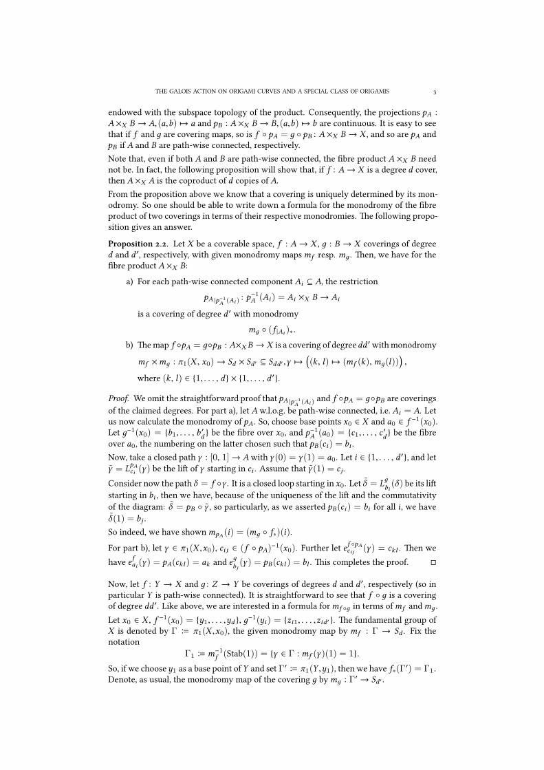
endowed with the subspace topology of the product. Consequently, the projections pA :A ×X B → A,(a,b) 7→ a and pB : A ×X B → B,(a,b) 7→ b are continuous. It is easy to seethat if f and д are covering maps, so is f ◦ pA = д ◦ pB : A ×X B → X , and so are pA andpB if A and B are path-wise connected, respectively.Note that, even if both A and B are path-wise connected, the fibre product A ×X B neednot be. In fact, the following proposition will show that, if f : A→ X is a degree d cover,then A ×X A is the coproduct of d copies of A.From the proposition above we know that a covering is uniquely determined by its mon-odromy. So one should be able to write down a formula for the monodromy of the fibreproduct of two coverings in terms of their respective monodromies. e following propo-sition gives an answer.

Proposition .. Let X be a coverable space, f : A → X , д : B → X coverings of degreed and d ′, respectively, with given monodromy mapsmf resp. mд . en, we have for thefibre product A ×X B:

a) For each path-wise connected component Ai ⊆ A, the restrictionpA |p−1A (Ai ) : p

−1A (Ai ) = Ai ×X B → Ai

is a covering of degree d ′ with monodromymд ◦ (f |Ai )∗.

b) emap f ◦pA = д◦pB : A×X B → X is a covering of degreedd ′withmonodromy

mf ×mд : π1(X , x0)→ Sd × Sd ′ ⊆ Sdd ′ ,γ 7→((k , l) 7→ (mf (k),mд(l))

),

where (k , l) ∈ {1, . . . , d } × {1, . . . , d ′}.

Proof. We omit the straightforward proof that pA |p−1A (Ai ) and f ◦pA = д◦pB are coveringsof the claimed degrees. For part a), let A w.l.o.g. be path-wise connected, i.e. Ai = A. Letus now calculate the monodromy of pA. So, choose base points x0 ∈ X and a0 ∈ f −1(x0).Let д−1(x0) = {b1, . . . , b ′d } be the fibre over x0, and p−1A (a0) = {c1, . . . , c ′d } be the fibreover a0, the numbering on the laer chosen such that pB(ci ) = bi .Now, take a closed path γ : [0, 1]→ Awith γ (0) = γ (1) = a0. Let i ∈ {1, . . . , d ′}, and letγ = L

pAci (γ ) be the li of γ starting in ci . Assume that γ (1) = c j .

Consider now the path δ = f ◦γ . It is a closed loop starting in x0. Let δ = Lдbi(δ) be its li

starting in bi , then we have, because of the uniqueness of the li and the commutativityof the diagram: δ = pB ◦ γ , so particularly, as we asserted pB(ci ) = bi for all i , we haveδ(1) = bj .So indeed, we have shownmpA(i) = (mд ◦ f∗)(i).For part b), let γ ∈ π1(X ,x0), ci j ∈ (f ◦ pA)−1(x0). Further let e f ◦pAci j (γ ) = ckl . en wehave e fai (γ ) = pA(ckl ) = ak and eдbj (γ ) = pB(ckl ) = bl . is completes the proof. □

Now, let f : Y → X and д : Z → Y be coverings of degrees d and d ′, respectively (so inparticular Y is path-wise connected). It is straightforward to see that f ◦ д is a coveringof degree dd ′. Like above, we are interested in a formula formf ◦д in terms ofmf andmд .Let x0 ∈ X , f −1(x0) = {y1, . . . ,yd }, д−1(yi ) = {zi1, . . . ,zid ′ }. e fundamental group ofX is denoted by Γ B π1(X ,x0), the given monodromy map by mf : Γ → Sd . Fix thenotation

Γ1 B m−1f (Stab(1)) = {γ ∈ Γ :mf (γ )(1) = 1}.So, if we choosey1 as a base point ofY and set Γ′ B π1(Y ,y1), then we have f∗(Γ′) = Γ1.Denote, as usual, the monodromy map of the covering д bymд : Γ′ → Sd ′ .

FLORIAN NISBACH

Proposition .. In the situation described above, let γi , i = 1, . . . ,d , be right coset rep-resentatives of Γ1 in Γ, with γ1 = 1, such that e fyi (γi ) = y1. So, we have Γ =

·∪Γ1 · γi .

en, we have:mf ◦д(γ )(i, j) =

(mf (γ )(i),mд(ci (γ ))(j)

)Here, we denote ci (γ ) B (f∗)−1(γkγγ−1i ), k B mf (γ )(i)

Proof. Let γ ∈ π1(X ,x0), α B Lf ◦дzi j (γ ), and further let α(1) = e

f ◦дzi j (γ ) =: zi′j′ . We have

to determine (i ′, j ′).e path β B L

fyi (γ ) = д ◦ α has endpoint β(1) = ymf (γ )(i). In particular, we have

i ′ =mf (γ )(i).

Now, let us determine j ′. So let βν B Lfyν (γν ) be liings (for ν = 1, . . . , d). Remember

that by our choice of the numbering of the γν , we have βν (1) = efyν (γν ) = y1. Using the

notation k B mf (γ )(i), we can write β = β−1k ββi with unique β ∈ π1(Y ,y1). Indeed, wehave: β = βkββ

−1i = L

fy1(γkγγ

−1i ).

W.l.o.g. we have that the liing αi j B Lдzi j (βi ) has endpoint z1j , as we have chosenγ1 = 1,

and for i , 1 we can renumber the zi j , j = 1, . . . ,d ′.Denote α B L

дz1j (β) and l B mд(β(j)), then we have α = α−1kl ααi j , and because of

α(1) = z1mд(β(j))we get:

zi′j′ = ef ◦дzi j (γ ) = α(1) =

(α−1kl ααi j

)(1) = zkl

So finally, j ′ = l =mд(β)(j) =mд(βkββ−1i )(j) =mд(ci (γ ))(j). □

Before we move on, let us state a lemma on normal coverings, which will become handylater on and which the author has learned from Stefan Kühnlein.

Lemma .. Let f : X → Y , f ′ : X ′ → Y be coverings and д : Y → Z be a normal(so in particular connected) covering, and let Z be a Hausdorff space. If д ◦ f � д ◦ f ′,i.e. there is a homeomorphism ϕ : X → X ′ with д ◦ f = д ◦ f ′ ◦ ϕ, then there is a decktransformationψ ∈ Deck(д) such thatψ ◦ f = f ′ ◦ ϕ.

X X ′

Y Y

Z

ϕ

f f ′

ψ

д д

Proof. Choose z ∈ Z , y ∈ д−1(z), x ∈ f −1(y). If we denote x ′ := ϕ(x),y ′ := f ′(x ′),then by hypothesis y ′ ∈ д−1(z). So by normality of д, there is a deck transformationψ ∈ Deck(д) such thatψ (y) = y ′ (which is even unique). Of course,ψ ◦ f (x) = f ′ ◦ϕ(x),and we claim now that we haveψ ◦ f = f ′ ◦ ϕ globally.Consider the set A := {a ∈ X | ψ ◦ f (a) = f ′ ◦ ϕ(a)}. Clearly A , ∅ because x ∈ A. Also,it is closed in X because all the spaces are Hausdorff. We want to show now thatA is alsoopen. Because X is connected, this implies A = X and finishes the proof.So let a ∈ A, and let д(f (a)) ∈ U ⊆ Z be an admissible neighbourhood for both д ◦ fand д ◦ f ′ (and so particularly for д). Furthermore let V ⊆ д−1(U ) be the connectedcomponent containing f (a), andW ⊆ f −1(V ) the one containing a. Denote V ′ := ψ (V ),and by W ′ denote the connected component of f ′−1(V ′) containing ϕ(a). As it is not


clear by hypothesis thatW ′ =W ′′ := ϕ(W ), set W ′ :=W ′ ∩W ′′, which is still an openneighbourhood of ϕ(a), and adjust the other neighbourhoods in the following way:

W := ϕ−1(W ′) ⊆W , V := f (W ), V ′ := f ′(W ′).

Note that we still have a ∈ W , that all these sets are still open, that U := д(V ) = д(V ′),and that the laer is still an admissible neighbourhood forд◦ f andд◦ f ′. By construction,by restricting all the maps to these neighbourhoods we get a commutative pentagon ofhomeomorphisms, so in particular (ψ ◦ f ) |W = (f ′ ◦ϕ) |W , which finishes the proof. □

. D ’ B’

Let us now establish the basic theory of dessins d’enfants. First, we give their definitionand explain Grothendieck’s equivalence to Belyi pairs, which we can, by GAGA, eithersee algebraically or analytically. en, we state Belyi’s famous theorem to establish theaction of Gal(� /�) on dessins and introduce the notions of fields of moduli and fields ofdefinitions of the appearing objects.We will mainly use the language of schemes in the context of algebraic curves, whichseems to be the natural viewpoint here in the eyes of the author. Our notation will staywithin bounds of the ones in the beautiful works [Wol], [Sch] and [Köc], in whichthe curious reader will find many of the details omied here.

.. Dessins and Belyi morphisms.

Definition .. a) A dessin d’enfant (or Grothendieck dessin, or children’s drawing)of degree d is a tuple (B,W ,G,S), consisting of:• A compact oriented connected real 2-dimensional (topological) manifold S ,• two finite disjoint subsets B,W ⊂ S (called the black and white vertices),• an embedded graph G ⊂ S with vertex set V (G) = B

.∪W which is bipartite

with respect to that partition of V (G), such that S \ G is homeomorphic toa finite disjoint union of open discs (called the cells of the dessin, and suchthat |π0(G \ (B ∪W ))| = d .

b) An isomorphism between two dessins D := (B,W ,G,S) and D ′ := (B′,W ′,G ′,S ′)is an orientation preserving homeomorphism f : S → S ′, such that

f (B) = B′, f (W ) =W ′, and f (G) = G ′.

c) By Aut(D) we denote the group of automorphisms of D, i.e. the group of isomor-phisms between D and itself.

So, from a naïve point of view, a dessin is given by drawing several black and white dotson a surface and connecting them in such a manner by edges that the cells which arebounded by these edges are simply connected. e starting point of the theory of dessinsd’enfants is that there are astonishingly many ways of giving the data of a dessin up toisomorphism. In the following proposition, we will survey several of these equivalences.

Proposition .. Giving a dessin in the above sense up to isomorphism is equivalent togiving each of the following data:

a) A finite topological covering β : X ∗ → ��\{0, 1, ∞} of degree d up to equiva-

lence of coverings.b) A conjugacy class of a subgroup G ≤ π1(�

�\{0, 1, ∞}) of index d .

c) A pair of permutations (px , py) ∈ S2d , such that ⟨px , py⟩ ≤ Sd is a transitivesubgroup, up to simultaneous conjugation in Sd .

d) A non-constant holomorphic map β : X → ��of degree d , where X is a com-

pact Riemann surface and β is ramified at most over the set {0, 1, ∞}, up to fibrepreserving biholomorphic maps.

FLORIAN NISBACH

e) A non-constant morphism β : X → ��of degree d , where X is a nonsingular

connected projective curve over � and β is ramified at most over the set {0, 1, ∞},up to fibre preserving �-scheme isomorphisms. Such a morphism is called a Belyimorphism.

Sketch of a proof. e crucial point is the equivalence between an isomorphism class ofdessins in the sense of the definition, and a conjugacy class of a pair of permutations asin c). It is shown by C. Voisin and J. Malgoire in [VM], and, in a slight variation, by G.Jones and D. Singerman in [JS, § ].e equivalence of a), b) and c) is a simple consequence of Proposition ., as the funda-mental group of �

�\{0, 1, ∞} is free in two generators x andy and the two permutations

px and py describe their images under the monodromy map.e equivalence between a) and d) is well-known in the theory of Riemann surfaces: ecomplex structure on �

�is unique, and every topological covering gives rise to a unique

holomorphic covering (compactness coming from metric completion).Finally, the equivalence between d) and e) follows from the well-known GAGA principlefirst stated in [Ser]. □

Let us illustrate these equivalences a lile more: First, note that reconstructing a dessinin the sense of Definition . from d) can be understood in the following explicit way:As S , we take of course the Riemann surface X , as B andW we take the preimages of 0and 1, respectively, and for the edges of G we take the preimages of the open interval(0,1) ⊂ �

�. en, S \ G is the preimage of the set �

�\[0, 1], which is open and simply

connected. So the connected components of S \G are open and simply connected propersubsets of a compact surface and thus homeomorphic to an open disc.Second, this indicates how to get from a dessin to the monodromy of the correspondingcovering: As generators of π1(�

�\{0, 1, ∞}), we fix simple closed curves around 0 and 1

with winding number 1 (say, starting in 12 ), and call them x and y, respecively. Choose a

numbering of the edges of the dessin. en, px consists of the cycles given by listing theedges going out of each black vertex in counter-clockwise direction, and we get py in thesame manner from the white vertices.Before we continue, we will state an easy consequence of Proposition .:

Corollary .. For any d ∈ �, there are only finitely many dessins d’enfants of degree dup to equivalence.

Proof. By Proposition ., a dessin can be characterised by a pair of permutations (px , py) ∈(Sd )

2. So, (d!)2 is an upper bound for the number of isomorphism classes of dessins ofdegree d . □

Next, we will establish the notion of a weak isomorphism between dessins.

Definition .. We call two Belyi morphisms β : X → ��and β ′ : X ′ → �

�weakly

isomorphic if there are biholomorphic ϕ : X → X ′ and ψ : ��→ �

�such that the

following square commutes:

X X ′

��

��

ϕ

β β ′

ψ

Note that in the above definition, if β and β ′ are ramified exactly over {0, 1, ∞}, then ψhas to be a Möbius transformation fixing this set. is subgroupW ≤ Aut(�

�) is clearly


isomorphic to S3 and generated bys : z 7→ 1 − z and t : z 7→ z−1.

In the case of two branch points, ψ can of course still be taken from that group. So fora dessin β , we get up to isomorphism all weakly isomorphic dessins by postcomposingwith all elements ofW . Let us reformulate this on a more abstract level:

Definition and Remark .. a) e groupW acts on the set of dessins from the lebyw ·β := w◦β . e orbits under that action are precisely the weak isomorphismclasses of dessins.

b) For a dessin β we call (by slight abuse of the above definition)Wβ := Stab(β), itsstabiliser inW , the group of nontrivial weak automorphisms.

c) If a dessin β is given by a pair of permutation (px , py), then its images under theaction ofW are described by the following table (where pz := p−1x p−1y ):

β s · β t · β (s ◦ t) · β (t ◦ s) · β (t ◦ s ◦ t) · β(px , py) (py , px ) (pz , py) (py , pz) (pz , px ) (px , pz)

Proof. Part a) was already discussed above. Proving c) amounts to checking what s andt do, and then composing and using ., for example. e calculation has been done in[Sij, p. .]. □

Let us now explain the common notions of pre-clean and clean dessins and introduce aterm for particularly un-clean ones:

Definition and Remark .. Let β be a dessin defined by a pair of permutations (px , py).

a) β is called pre-clean if p2y = 1, i.e. if all white vertices are either of valence 1 or 2.b) β is called clean if all preimages of 1 are ramification points of order precisely 2,

i.e. if all white vertices are of valence 2.c) If β : X → �

�is a Belyi morphism of degree d , then if we define a(z) :=

4z(1 − z) ∈ �[z] we find that a ◦ β is a clean dessin of degree 2d .d) We will call β filthy if it is not weakly isomorphic to a pre-clean dessin, i.e. 1 <{p2x , p2y , p2z }.

Another common class of dessins consists of the unicellular ones. We briefly discuss themhere.

Definition and Remark .. a) A dessin d’enfant D is said to be unicellular if it con-sists of exactly one open cell.

b) If D is represented by a pair of permutations (px , py), it is unicellular iff pz =p−1x p−1y consists of exactly one cycle.

c) If D is represented by a Belyi morphism β : X → ��, it is unicellular iff β has

exactly one pole.d) If D is a dessin in genus 0, it is unicellular iff its graph is a tree.

.. Fields of definition, moduli fields and Belyi’s theorem. Let us recall the notions offields of definition and moduli fields of schemes, varieties and morphisms. Following thethreat in the beginning of this section and the presentation of this material in [Köc],we will use the language of schemes.By Spec, denote the usual spectrum functor from commutative rings to affine schemes.Fix a field K . Remember that a K-scheme is a pair (S ,p), where S is a scheme andp : S → Spec(K) a morphism. (S ,p) is called K-variety if S is reduced and p is a sepa-rated morphism of finite type. A morphism between K-schemes is a scheme morphismforming a commutative triangle with the structure morphisms. Denote the such obtainedcategories by Sch/K and Var/K , respectively.

FLORIAN NISBACH

Keep in mind that p is part of the data of a K-scheme (S ,p), and that changing it gives adifferent K-scheme even though the abstract scheme S stays the same. is allows us todefine an action of Aut(K) on Sch/K :

Definition and Remark .. Let (S ,p) be a K-scheme, and σ ∈ Aut(K).a) Define (S ,p)σ := (S ,Spec(σ) ◦ p).b) Mapping (S ,p) 7→ (S ,p)σ defines a right action of Aut(K) on Sch/K . is restricts

to an action on Var/K .

We are now able to define the terms field of definition and moduli field.

Definition .. a) A subfield k ⊆ K is called afield of definition of a K-scheme (K-variety) (S ,p) if there is a k-scheme (k-variety) (S ′,p ′) such that there is a Carte-sian diagram

S S ′

□

Spec(K) Spec(k)

p p′

Spec(ι)

where ι : k → K is the inclusion. Alternatively, (S ,p) is said to be defined over kthen.

b) For a K-scheme (S ,p), define the following subgroupU (S ,p) ≤ Aut(K):U (S ,p) := {σ ∈ Aut(K) | (S ,p)σ � (S ,p)}

e moduli field of (S ,p) is then defined to be the fixed field under that group:

M(S ,p) := KU (S,p)

Wewill also need to understand the action of Aut(K) onmorphisms. Wewill start the badhabit of omiing the structure morphisms here, which the reader should amend mentally.

Definition .. Let β : S → T be a K-morphism (i.e. a morphism of K-schemes) andσ ∈ Aut(K).

a) e scheme morphism β is of course also a morphism between the K-schemes Sσand T σ . We denote this K-morphism by βσ : Sσ → T σ .

b) Let β ′ : S ′ → T ′ be another K-morphism. en we write β � β ′ if there areK-isomorphisms ϕ : S → S ′ andψ : T → T ′ such thatψ ◦ β = β ′ ◦ϕ. Specifically,we have β � βσ iff there are K-morphisms ϕ,ψ such that the following diagram(where we write down at least some structure morphisms) commutes:

Sσ S

T σ T

Spec(K) Spec(K)

ϕ

βσ β

ψ

p p

Spec(σ )

Let us now define the field of definition and the moduli field of a morphism in the samemanner as above. For an inclusion ι : k → K denote the corresponding base changefunctor by · ×Spec(k) Spec(K).


Definition .. a) A morphism β : S → T of K-schemes (or K-varieties, respec-tively) is said to be defined over a field k ⊆ K if there is a morphism β ′ : S ′ → T ′

of k-schemes (k-varieties) such that β = β ′ ×Spec(k) Spec(K).b) For a morphism β : S → T of K-schemes, define the following subgroup U (β) ≤

Aut(K):U (β) := {σ ∈ Aut(K) | βσ � β }

e moduli field of β is then defined to be the fixed field under this group:M(β) := KU (β)

If, now, β : X → ��is a Belyi morphism, the above notation gives already a version for

a moduli field of β . But this is not the one we usually want, so we formulate a differentversion here:Definition .. Let β : X → �

�be a Belyi morphism, and let Uβ ≤ Aut(�) be the

subgroup of field automorphisms σ such that there exists a �-isomorphism fσ : Xσ → Xsuch that the following diagram commutes:

Xσ X

(��)σ �

�

fσ

βσ β

Proj(σ )

where Proj(σ) shall denote the scheme (not�-scheme!) automorphism of��= Proj(�[X0, X1])

associated to the ring (not �-algebra!) automorphism of �[X0, X1] which extends σ ∈Aut(�) by acting trivially on X0 and X1.en, we call the fixed fieldMβ := �Uβ the moduli field of the dessin corresponding to β .

e difference to Definition . b) is that there, we allow composing Proj(σ) with auto-morphisms of �

�, potentially making the subgroup of Aut(�) bigger and therefore the

moduli field smaller. Let us make that precise, and add some more facts about all thesefields, by citing [Wol, Proposition ]:Proposition .. Let K be a field, and β : S → T a morphism of K-schemes, or ofK-varieties. en:

a) M(S) and M(β) depend only on the K-isomorphism type of S resp. β .b) If furthermore β is a Belyi morphism, then the same goes for Mβ .c) Every field of definition of S (resp. β) contains M(S) (resp. M(β)).d) We have M(S) ⊆ M(β).e) If β is a Belyi morphism, then we also have M(β) ⊆ Mβ .) In this case Mβ (and therefore also M(S) and M(β)) is a number field, i.e. a finite

extension of �.

Proof. Parts a) to e) are direct consequences of the above definitions, and for ) we notethat surely if σ ∈ Aut(�) then deg(β) = deg(βσ ). So by Corollary ., we have [Aut(�) :Uβ ] = |β · Aut(�)| < ∞ and so [Mβ : �] < ∞. □

We can now state Belyi’s famous theorem:eorem (V. G. Belyi). LetC be a smooth projective complex curve. C is definable overa number field if and only if it admits a Belyi morphism β : C → �

�.

In our scope, the gap between Proposition . ) and the “i” part (traditionally called the“obvious” part) of the theorem can be elegantly filled by the following theorem that canbe found in [HH]:

FLORIAN NISBACH

eorem (H. Hammer, F. Herrlich). Let K be a field, and X be a curve over K . en Xcan be defined over a finite extension of M(X ).

e “only i” (traditionally called “trivial”) part of the theorem is a surprisingly explicitcalculation of which several variations are known. e reader may refer to Section . of[GG].

.. e action of Gal(� /�) on dessins. Given a Belyi morphism β : X → ��and an

automorphism σ ∈ Aut(�), in fact βσ : Xσ → ��is again a Belyi morphism, as the

number of branch points is an intrinsic property of the underlying scheme morphism βthat is not changed by changing the structure morphisms. So, Aut(�) acts on the set ofBelyi morphisms, and so, due to Proposition ., on the set of dessins d’enfants. By Belyi’stheorem, this action factors through Gal(� /�). It turns out that this action is faithful.Let us state this well known result in the following

eorem . For every д ∈ �, the action of Gal(� /�) on the set of dessins d’enfants ofgenusд is faithful. is still holds for everyд if we restrict to the clean, unicellular dessinsin genus д.

In genus 1, this can be seen easily as the action defined above is compatible with thej-invariant, i.e. we have σ((j(E))) = j(Eσ ) for an elliptic curve E. It was noted by F.Armknecht in [Arm] that this argument generalises to higher genera, by even restrict-ing to hyperelliptic curves only.e standard proof for genus 0 can be found in [Sch], where it is aributed to H. W.Lenstra, Jr. e result there even stronger than the claim here, as it establishes the faith-fulness of the action even on trees.e fact that the faithfulness does not break when restricting to unicellular and cleandessins can be proven easily by carefully going through the proof of the “trivial” part ofBelyi’s theorem—see [Nis, Proof of eorem G] for details.

. O T

.. Origamis as coverings. Here, we will the exhibit the definition of an Origami firstin the spirit of the previous section and then in the scope of translation surfaces. We willthen present a short survey of the theory of translation surfaces and Teichmüller curves,and finally speak about arithmetic aspects of all these objects.e term “Origami” was coined by P. Lochak—see [Loc] and be aware that it is used ina slightly different meaning there.e standard intuition for constructing an Origami of degreed ∈ � is the following: Taked copies of the unit square [0, 1] × [0, 1] and glue upper edges to lower edges and le toright edges, respecting the orientation, until there are no free edges le, in a way that wedo not end up with more than one connected component. In this way, we get a compacttopological surfaceX together with a tiling intod squares (hence the other common namefor Origamis: square tiled surfaces).Such a tiling naturally defines a (ramified) covering p : X → E of the unique Origami ofdegree 1, which we call E, i.e. a compact surface of genus 1, by sending each square of Xto the unique square of E. p is ramified over one point, namely the image under glueingof the vertices of the square.To bemore exact, fix E B � /�2 (this defines a complex structure on E), thenp is ramified(at most) over 0 + �2. Denote this point by∞ for the rest of this work, and furthermoreE∗ B E \ {∞}, X ∗ B X \ p−1(E∗). Note that p : X ∗ → E∗ is an unramified covering ofdegree d , and the fundamental group of E∗ is free in two generators, so one should expectanalogies to the world of dessins. Let us write down a proper definition:


Definition .. a) AnOrigamiO of degreed is an unramified coveringO B (p : X ∗ →E∗) of degree d , where X ∗ is a (noncompact) topological surface.

b) If O ′ = (p ′ : X ′∗ → E∗) is another Origami, then we say that O is equivalent toO ′ (which we denote by O � O ′), if the defining coverings are isomorphic, i.e. ifthere is a homeomorphism ϕ : X ′∗ → X ∗ such that p ′ = p ◦ ϕ.

c) O = (p : X ∗ → E∗) is called normal if p is a normal covering.

Like in the case of dessins, this is not the only possible way to define an Origami. We listseveral others here:

Proposition .. Giving an Origami in the above sense up to equivalence is equivalent togiving each of the following data:

a) A conjugacy class of a subgroup G ≤ π1(E∗) � F2 of index d .b) A pair of permutations (pA, pB) ∈ S2d , such that ⟨pA, pB⟩ ≤ Sd is a transitive

subgroup, up to simultaneous conjugation in Sd .c) A non-constant holomorphic map p : X → E of degree d , where X is a compact

Riemann surface and p is ramified at most over the set {∞}, up to fibre preservingbiholomorphic maps.

d) A non-constant morphism p : X → E of degree d , where X is a nonsingularconnected projective curve over � and p is ramified at most over the set {∞}, upto fibre preserving isomorphisms.

e proof is completely analogous to the one of Proposition .. See [Kre, Proposition.] for details.

.. Origamis and translation surfaces. As we want to study Origamis as translationsurfaces, let us briefly recall their theory.

Definition .. Let X be a Riemann surface, and let X be its complex structure.

a) A translation structure µ onX is an atlas compatible withX (as real analytic atlases,i.e. their union is an atlas of a real analytic surface), such that for any two chartsf , д ∈ µ, the transition map is locally a translation, i.e. a map

ϕf ,д : U ⊆ �→ U ′ ⊆ �, x 7→ x + tf ,д

for some tf ,д ∈ �. We call the pair Xµ B (X , µ) a translation surface.b) A biholomorphic map f : Xµ → Yν between translation surfaces is called a trans-

lation, or an isomorphism of translation surfaces, if it is locally (i.e. on the level ofcharts) a translation. Xµ and Yν are then called isomorphic (as translation sur-faces). If in this case X = Y , we say that the translation structures µ and ν areequivalent.

c) If µ is a translation structure onX , andA ∈ SL2(�), then we define the translationstructure

A · µ B {A · f | f ∈ µ}where A shall act on � by identifying it with �2 as usual. erefore, we get a leaction of SL2(�) on the set of translation structures on X .

Keep in mind that a translation structure µ on X , seen as a complex structure, is usuallynot equivalent to X!Let us go on by defining affine diffeomorphisms and the notion of the Veech group of atranslation surface:

Definition and Remark .. Let Xµ , Yν be translation surfaces.

FLORIAN NISBACH

a) An affine diffeomorphism f : Xµ → Yν is an orientation preserving diffeomor-phism such that locally (i.e. when going down into the charts) it is a map of theform

x 7→ A · x + t , A ∈ GL2(�), t ∈ � .We call Xµ and Yν affinely equivalent if there is such an affine diffeomorphism.

b) e matrix A =: Af in a) actually is a global datum of f , i.e. it is the same forevery chart. We write der(f ) B Af .

c) An affine diffeomorphism f is a translation iff Af = I .d) If д : Yν → Zξ is another affine diffeomorphism, then der(д◦ f ) = der(д) ·der(f ),

i.e. der : Aff+(Xµ )→ GL2(�), is a group homomorphism.e) We denote the group of all affine orientation preserving diffeomorphisms from

Xµ to itself by Aff+(Xµ ).) Trans(Xµ ) B ker(der) is called the group of translations of Xµ .g) Γ(Xµ ) B im(der) is called the Veech group of Xµ . Its image under the projection

map GL2(�)→ PGL2(�) is called the projective Veech group of Xµ . We denote itby PΓ(Xµ ).

h) If A ∈ SL2(�), then we have A ∈ Γ(Xµ )⇔ Xµ � XA ·µ as translation surfaces.

For a discussion of this, see [Sch, Section .].Note that if (Xµ ) has finite volume, every affine diffeomorphism has to preserve the vol-ume, and as we require affine affine diffeomorphisms also to preserve the orientation, thisyields Γ(Xµ ) ⊆ SL2(�).Our model genus 1 surface E = � /�2 carries a natural translation structure µ0, as �2

acts on� by translations. It is quite easy to see that the Veech groupΓ(Eµ0) is themodulargroup SL2(�): Denote by π : � → E the projection, then every affine diffeomorphismon E lis to a globally affine transformation on � via π . On the other hand, a matrixA ∈ SL2(�) induces an affine diffeomorphism on E if and only if it respects the laice �2,i.e. iff A ∈ SL2(�). Analogously, for B ∈ SL2(�), the veech group of � /(B · �2) (with atranslation structure µB obtainend in the same way as above) is B SL2(�)B−1. Also, wehave Γ(EB ·µ0) = B SL2(�)B−1.Let us fix our favourite generators for SL2(�):

S :=

(0 −11 0

)and T :=

(1 10 1

).

Given a translation surface Xµ and a topological covering f : Y → X , we obtain a trans-lation structure f ∗µ on Y by precomposing small enough charts from µ by f . e mapp : Yf ∗µ → Xµ is then usually called translation covering. In this way, let us define theVeech group of an Origami:

Definition .. Let O = (p : X ∗ → E∗) be an Origami. en we callΓ(O) := Γ(X ∗, p∗µ0)

the Veech group of O .

Let us list some fundamental properties:

Proposition .. If O = (p : X ∗ → E∗) is an Origami, and Γ := Γ(O) its Veech group,then we have:

a) Γ ⊆ SL2(�).b) Γ(X ∗,B · p∗µ0) = BΓB−1 for every B ∈ SL2(�).c) e isomorphism classes of Origamis that are affinely equivalent to O are in bi-

jection with the le cosets of Γ in SL2(�).d) [SL2(�) : Γ] < ∞.


Proofs can be found in [Sch]: a) and b) can be found in Section . there; c) is elemen-tary if we use Schmithüsen’s Proposition . which states that any affine diffeomorphismX ∗ → X ′∗ descends to an affine diffeomorphism E∗ → E∗. Her Corollary . provides aproof for d). ough, part d) can be proven in a more elementary way, by noting that theSL2(�) action on Origamis O = (p : X ∗ → E∗) preserves the volume of X ∗ and thus thedegree of p. We can then conclude with the same argument as in Corollary ..To calculate the Veech groups of the special Origamis appearing later in this work, weuse a rather different characterisation of Veech groups of Origamis found by G. Weitze-Schmithüsen in [Sch]. Remember π1(E∗) � F2 and consider the group homomorphismϕ : Aut(π1(E∗)) → Out(π1(E∗)) � GL2(�). Via the laer isomorphism, we defineOut+(π1(E∗)) B SL2(�) and Aut+(π1(E∗) B ϕ−1(Out+(π1(E∗))). eir elements arecalled “orientation preserving” (outer) automorphisms.

eorem (G. Schmithüsen). Let O B (p : X ∗ → E∗) be an Origami. en we have:

a) Γ(O) = ϕ(Stab(p∗π1(X ∗))).b) If f ∈ Aut+(π1(E∗)), ϕ(f ) = A ∈ SL2(�), and the monodromy of O is given by

mp , then the monodromy of A ·O is given bymp ◦ f .

e first part iseorem in said work, the second is the isomorphism β from Proposition. there.

.. Moduli and Teimüller spaces of curves. We begin by giving a somewhat roughdefinition of different versions of the (coarse) moduli space of compact Riemann surfaces.A very detailed reference on this subject is provided in [HM].

Definition .. a) Define the coarse moduli space of Riemann surfaces of genusд withn distinguished marked points as

Mд,n :={(X , p1, . . . ,pn) | X compact R. s. of genusд, pi ∈ X , pi , pj for i , j

}/∼

where (X , p1, . . . ,pn) ∼ (Y , q1, . . . ,qn) if there is a biholomorphicmapϕ : X → Ywith ϕ(pi ) = qi , i = 1, . . . ,n.

b) Define the coarsemoduli space of Riemann surfaces of genusдwithn non-distinguishedmarked points as

Mд,[n] :={(X , p1, . . . ,pn) | X compact R. s. of genusд, pi ∈ X , pi , pj for i , j

}/∼

where (X , p1, . . . ,pn) ∼ (Y , q1, . . . ,qn) if there is a biholomorphic function ϕ :X → Y and a permutation π ∈ Sn , such that ϕ(pi ) = qπ (i), i = 1, . . . ,n.

c) Finally, define the coarse moduli space of Riemann surfaces of genus д as

Mд := Mд,0 = Mд,[0].

In fact, Mд,n and Mд,[n], which we defined just as sets, can be turned into complex quasi-projective varieties, or complex analytic spaces, of dimension 3д − 3 + n (whenever thisexpression is positive—we have dim(M1,0) = 1, and dim(M0,n) = 0 for n ≤ 3). ere arenatural projections

Mд,n → Mд,[n] → Mд

by forgeing the order of the marked points, and totally forgeing the marked points.All these versions also exist as schemes, which are all defined over �.e usual analytical approach to understanding moduli spaces is Teichmüller theory. Letus recall the basic facts. We begin by giving the definition of Teichmüller spaces:

Definition and Remark .. Let S be a fixed compact Riemann surface of genus д with nmarked points. (Let us write shortly that S is of type (д,n).)

FLORIAN NISBACH

a) If X is another surface of this type, a marking on X is an orientation preservingdiffeomorphism ϕ : S → X which respects the marked points.

b) We define the Teichmüller space of the surface S asT (S) B

{(X , ϕ) | X R. s. of type (д,n), ϕ : S → X a marking} /∼

where (X , ϕ) ∼ (Y , ψ ) if ψ ◦ ϕ−1 : X → Y is homotopic to a biholomorphism re-specting the marked points (where, of course, the homotopy shall fix the markedpoints).

c) If S ′ is another surface of type (д,n), then any choice of a marking on ϕ : S → S ′

yields a bijection T (S ′) → T (S) by precomposing all markings with ϕ, whichgives us the right to just write Tд,n .

In the same manner as above, there exist also versions with non-ordered and withoutmarked points, denoted by Tд,[n] and Tд , respectively. It turns out that Tд,n is a com-plex manifold of dimension 3д − 3 + n whenever this expression is positive. Actually,it is isomorphic to a unit ball of that dimension. e group of orientation preservingdiffeomorphisms of S , denoted by Diffeo+(S), acts on T (S) from the le by composi-tion with the marking. It is clear that this action factors over the mapping class groupΣ(S) B π0(Diffeo+(S)) and that its orbits are precisely the isomorphism types of Rie-mann surfaces of type (д,n), so that we have

T (S)/Σ(S) � Mд,n .

It is also true but far less obvious that Σ(S) acts properly discontinous and with finitestabilisers, and that the above equation holds in the category of complex spaces.Analogous statements hold for surfaces with n non-ordered marked points. Note thatcompact surfaces of genus д with finitely many points removed can be compactifieduniquely and is thus naturally an element of Mд,[n].

.. Teimüller discs and Teimüller curves. Let X be a compact Riemann surface ofgenus д with n punctures, endowed with a translation structure. For B ∈ SL2(�), denotebyXB the Riemann surface thatwe get by endowingX with the complex structure inducedby B · µ. en the identity map id : X = XI → XB is a marking in the sense of Definitionand Remark . a). Note that this map is in general not holomorphic! So we get a map

θ : SL2(�)→ Tд,[n], B 7→ [(XB , id : XI → XB)] .

Since for B ∈ SL2(�)we have that z 7→ B ·z is biholomorphic iff B ∈ SO(2) it is easy to seethatθ factors through SO(2)\ SL2(�) � �. (Fix the laer bijection asm : SO(2)\ SL2(�)→�, [A] 7→ −A−1(i). e reason for this choice become clear in a bit.) e factor map

θ : �→ Tд,[n]is injective. It is in fact biholomorphic, and furthermore an isometry with respect tothe standard hyperbolic metric on � and the Teichmüller metric on Tд,[n] as defined, forexample, in [Hub, p. .]. See [Nag, .. and ..] for details. is leads to thefollowingDefinition .. Let Xµ B (X , µ) be a translation surface of type (д, [n]). en, the iso-metric image

∆Xµ B θ(�) ⊆ Tд,[n]is called the Teichmüller disc associated with Xµ .

e image of a Teichmüller disc ∆Xµ under the projection map into moduli space is, ingeneral, not be an algebraic subvariety. If the Veech group of the translation surfaceXµ isa laice in SL2(�), i.e. if vol(� /Γ(Xµ )) < ∞, then in fact the image of∆Xµ in the modulispace is an algebraic curve, as stated in the following theorem. It is usually aributed toJohn Smillie, but cited from [McM].


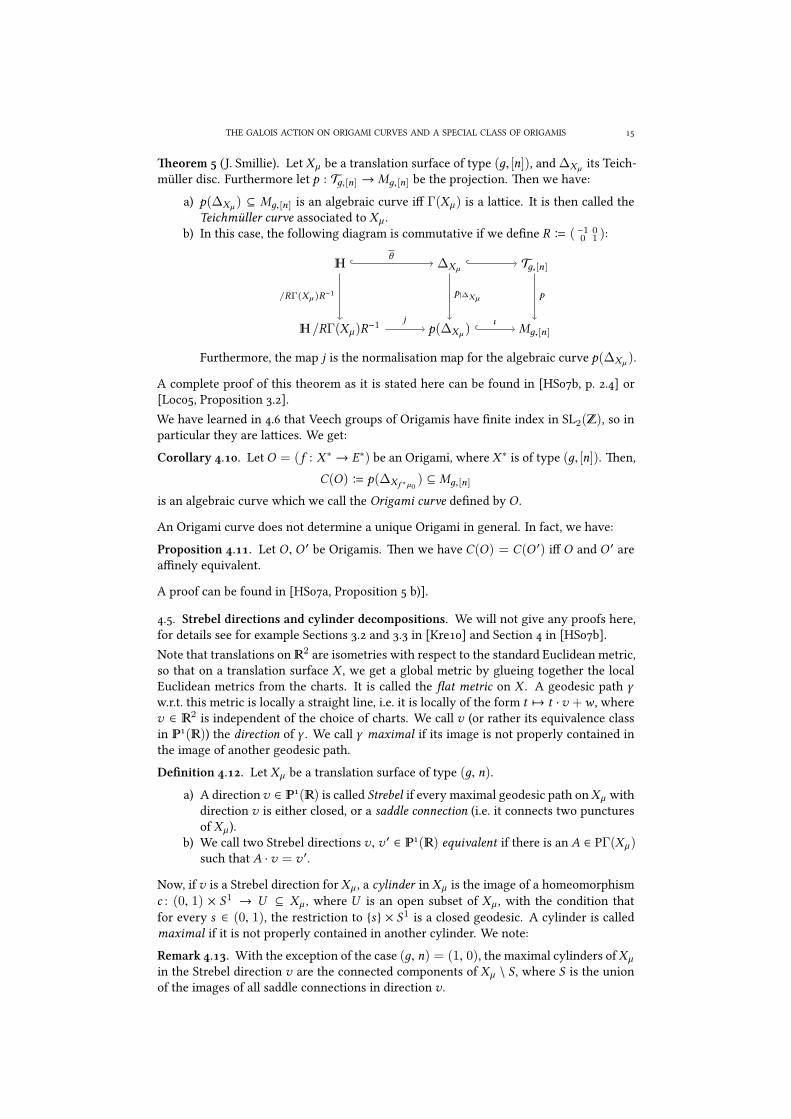
eorem (J. Smillie). Let Xµ be a translation surface of type (д, [n]), and ∆Xµ its Teich-müller disc. Furthermore let p : Tд,[n] → Mд,[n] be the projection. en we have:

a) p(∆Xµ ) ⊆ Mд,[n] is an algebraic curve iff Γ(Xµ ) is a laice. It is then called theTeichmüller curve associated to Xµ .

b) In this case, the following diagram is commutative if we define R B ( −1 00 1 ):

� ∆Xµ Tд,[n]

� /RΓ(Xµ )R−1 p(∆Xµ ) Mд,[n]

θ

/RΓ(Xµ )R−1 p |∆Xµ p

j ι

Furthermore, the map j is the normalisation map for the algebraic curve p(∆Xµ ).

A complete proof of this theorem as it is stated here can be found in [HSb, p. .] or[Loc, Proposition .].We have learned in . that Veech groups of Origamis have finite index in SL2(�), so inparticular they are laices. We get:Corollary .. LetO = (f : X ∗ → E∗) be an Origami, where X ∗ is of type (д, [n]). en,

C(O) B p(∆Xf ∗µ0) ⊆ Mд,[n]

is an algebraic curve which we call the Origami curve defined by O .

An Origami curve does not determine a unique Origami in general. In fact, we have:Proposition .. Let O , O ′ be Origamis. en we have C(O) = C(O ′) iff O and O ′ areaffinely equivalent.

A proof can be found in [HSa, Proposition b)].

.. Strebel directions and cylinder decompositions. We will not give any proofs here,for details see for example Sections . and . in [Kre] and Section in [HSb].Note that translations on�2 are isometries with respect to the standard Euclidean metric,so that on a translation surface X , we get a global metric by glueing together the localEuclidean metrics from the charts. It is called the flat metric on X . A geodesic path γw.r.t. this metric is locally a straight line, i.e. it is locally of the form t 7→ t ·v +w , wherev ∈ �2 is independent of the choice of charts. We call v (or rather its equivalence classin �(�)) the direction of γ . We call γ maximal if its image is not properly contained inthe image of another geodesic path.Definition .. Let Xµ be a translation surface of type (д, n).

a) A directionv ∈ �(�) is called Strebel if every maximal geodesic path onXµ withdirection v is either closed, or a saddle connection (i.e. it connects two puncturesof Xµ ).

b) We call two Strebel directions v, v ′ ∈ �(�) equivalent if there is an A ∈ PΓ(Xµ )such that A · v = v ′.

Now, if v is a Strebel direction for Xµ , a cylinder in Xµ is the image of a homeomorphismc : (0, 1) × S1 → U ⊆ Xµ , where U is an open subset of Xµ , with the condition thatfor every s ∈ (0, 1), the restriction to {s} × S1 is a closed geodesic. A cylinder is calledmaximal if it is not properly contained in another cylinder. We note:Remark .. With the exception of the case (д, n) = (1, 0), the maximal cylinders ofXµin the Strebel direction v are the connected components of Xµ \ S , where S is the unionof the images of all saddle connections in direction v .

FLORIAN NISBACH

Let us restrict to Origamis now and summarise the situation in this case:Proposition .. Let O = (p : X ∗ → E∗) be an Origami. en we have:

a) ere is a bijection between the following sets:• Equivalence classes of Strebel directions of O ,• Conjugacy classes of maximal parabolic subgroups in PΓ(O),• Punctures (called cusps) of the normalisation of theOrigami curve,� /RΓ(O)R−1.

b) e vector ( 10 ) is a Strebel direction of O , called its horizontal Strebel direction.c) Any maximal parabolic subgroup of PΓ(O) is generated by the equivalence class

of a matrix of the form дTwд−1, for somew ∈ �, д ∈ SL2(�).d) e Strebel direction corresponding to a maximal parabolic subgroup ⟨дTwд−1⟩ is

vд B д ·( 10 ). e maximal cylinders ofO in this Strebel direction are the maximalhorizontal cylinders of the Origami д−1 ·O .

Proofs can be found in Sections . and . of [Kre].

.. e action of Gal(� /�) on Origami curves. As the way we constructed Teich-müller curves is clearly of analytical nature, it may be surprising that they have inter-esting arithmetic properties. is kind of connection reminds of the eorem of Belyi,which we can indeed use to prove a small part of the followingProposition .. Let O = (p : X ∗ → E∗) be an Origami and C(O) ⊆ Mд,[n] its Teich-müller curve.

a) en, the normalisation map j : � /R−1Γ(O)R → C(O) and the inclusion ι :C(O) ↪→ Mд,[n] are defined over number fields.

b) Let σ ∈ Gal(� /�) be a Galois automorphism, and Oσ = (pσ : (X ∗)σ → E∗) theGalois conjugate Origami*. en we have†

ισ ((C(O))σ ) = ι(C(Oσ )) ⊆ Mд,[n],

so in particular C(Oσ ) � (C(O))σ .

is result is proven by Möller in [Möl, Proposition .]. e main ingredient to hisproof is the fact that HE , the Hurwitz stack of coverings of elliptic curves ramified overone prescribed point of some prescribed genus and degree, is a smooth stack defined over�. is is a result of Wewers that can be found in [Wew]. One identifies (an orbifoldversion o) C(O) as a geometric connected component of HE . e Gal(� /�)-orbit ofC(O) consists precisely of the geometric connected components of the �-connected com-ponent containingC(O). e definability ofC(O) over a finite extension of� then followsfrom the fact thatHE has only finitely many geometric connected components. Showingthis amounts to showing that the number or Origamis of given degree is finite.For a more detailed account of the proof of part b) than in [Möl], see [Nis, Section.].e desired Galois action on Origami curves is a direct consequence of Proposition .:Corollary .. Let O be a set containing one Origami of each isomorphism type. enthere is a natural right action of Gal(� /�) on the set

C(O) B {C(O) | O ∈ O},where σ ∈ Gal(� /�) sends C(O) to C(Oσ ).

*Note here that we fixed the choice of E = � /�2. We have j(E) = 1728 ∈ �, and thus E is defined over�.

†Strictly speaking, we should use a notation like ιC(O) to distinguish the embeddings of different Origamicurves. We suppress the index for reasons of simplicity and bear in mind that the following formula has twodifferent morphisms called ι .


.. Galois invariants andmoduli fields. Let us now return to the notion ofmoduli fields,which we defined in .. We begin by defining the moduli field of an Origami, and of anOrigami curve:

Definition .. Let O = (p : X ∗ → E∗) be an Origami, and C(O) its Origami curve.

a) Consider the following subgroup of Aut(�):

U (O) B{σ ∈ Aut(�) | ∃� -isomorphism ϕ : Xσ → X : pσ = p ◦ ϕ}

en, M(O) B �U (O) is called the moduli field of O .b) Remember that Mд,[n] is defined over � and define

U (C(O)) B{σ ∈ Aut(�) | C(O) = (C(O))σ

},

where as usual we considerC(O) and (C(O))σ as subsets ofMд,[n]. en, we callM(C(O)) B �U (C(O)) the moduli field of the Origami curve C(O).

Let us first note some easy to prove properties of these moduli fields:

Remark .. Let, again, O = (p : X ∗ → E∗) be an Origami, and C(O) its Origami curve.en we have:

a) M(C(O)) ⊆ M(O).b) [M(O) : �] = |O · Aut(�)| < ∞ and [M(C(O)) : �] = |C(O) · Aut(�)| < ∞.

Proof. Part a) is a consequence of Corollary .: If σ ∈ Aut(�) fixes O , it particularlyfixes C(O).For part b) we begin by noting that we have |O · Aut(�)| < ∞ because the degree of Ois an invariant under the action of Aut(�), and, as we have seen before, we can boundthe number of Origamis of degree d by (d!)2. Furthermore, we have [Aut(�) : U (O)] =|O · Aut(�)|, as U (O) is the stabiliser of O under the action of Aut(�). From [Köc,Lemma .] follows the equality [M(O) : �] = [Aut(�) : U (O)], given that we can showthat U (O) is a closed subgroup of Aut(�). Remember that a subgroup G ≤ Aut(�) isclosed iff there is a subfield F ⊆ �withG = Aut(� /F ). Lemma . in the same article tellsus thatU (O) is closed if there is a finite extension D/M(O) such that Aut(� /D) ≤ U (O).Let us now give a reason for the existence of such an extension D: As E and the branchlocus {∞} are defined over�, it follows from [Gon, eorem .] that p : X → E can bedefined over a number field. Choose such a field of definition D, which is hence a finiteextension of M(O). Obviously, any element σ ∈ Aut(�) that fixes D lies in U (O), so wecan apply Köck’s Lemma . and finally deduce the first half of b).Now we restate these arguments for the second equality: We use a) to deduce [M(C(O)) :�] < ∞. Furthermore, from Proposition . a) follows that the embedded Origami curveC(O) can be defined over a number field, so we can use the same chain of arguments asabove. □

It is interesting to know which properties of Origamis are Galois invariants. Let us listsome fairly obvious ones:

eorem . e following properties of an OrigamiO = (p : X ∗ → E∗) are Galois invari-ants:

a) e index of the Veech group [SL2(�) : Γ(O)].b) e index of the projective Veech group [PSL2(�) : PΓ(O)].c) e property whether or not −I ∈ Γ(O).d) e isomorphism type of the group of translations, Trans(O).

FLORIAN NISBACH

is has surely been noticed before, but in lack of a beer reference we refer to [Nis,Section .] for a proof.As an application, we can bound the degree of the field extension M(C(O))/M(O) fromabove in a way that looks surprising at first:

eorem . Let O = (p : X ∗ → E∗) be an Origami. en we have

[M(O) : M(C(O))] ≤ [SL2(�) : Γ(O)].

Proof. Let O · Aut(�) = {O1, . . . , Ok } and C(O) · Aut(�) = {C1, . . . , Cl }. en we have,as we have shown in Remark . b):

k = [M(O) : �], l = [M(C(O)) : �].

By eorem the Veech groups of all Oi have the same indexm B [SL2(�) : Γ(O)], andby Corollary . we also have

{C1, . . . , Cl } = {C(O1), . . . , C(Ok )}.

From Proposition . c) we know that each curveCj can be the Origami curve of at mostm of the Oi ’s, so we have

l ≥ k

m,

or equivalently kl ≤ m. e le hand side of the laer inequality is by the multiplicity

of degrees of field extensions equal to [M(O) : M(C(O))], and the right hand side is bydefinition the index of the Veech group of O . □

. T G MO

e goal of this section is to recreate M. Möller’s construction of Origamis from dessins,which he used to prove the faithfulness of the Galois action on Origami curves in [Möl],in a more topological way. at is, we will calculate the monodromy of these Origamis(called M-Origamis here) as well as their cylinder decompositions and Veech groups, andwe will reprove said faithfulness result in a way explicit enough to give examples of non-trivial Galois orbits.

.. Pillow case Origamis and M-Origamis. Remember the elliptic curve of our choiceE = � /�2 and that it is defined over �. It carries a group structure; denote its neutralby∞ B 0+�2. Further denote by [2] : E → E the multiplication by 2, and by h : E → �

�

the quotient map under the induced elliptic involution z + �2 7→ −z + �2. e map hshall be chosen such that h(∞) = ∞, and that the other critical values are 0, 1 and someλ ∈ �. By abuse of notation, call their preimages also 0, 1 and λ. By even more abuse ofnotation, call {0, 1 λ,∞} ⊂ E the set of Weierstraß points and recall that it is the kernelof [2]. Note that [2] is an unramified covering of degree 4, and h is a degree 2 coveringramified over {0, 1, λ,∞}.Now let γ : Y → �

�be a connected pillow case cover. at is, let Y be a nonsingular con-

nected projective curve over �, and γ a nonconstant morphism with critγ ⊆ {0,1,λ,∞}.Let π : X B E ×�

�Y → E be its pullback by h, and δ : X → X be the desingularisation of

X (as X will have singularities in general—we will discuss them later in this section). Fi-nally, consider the map let [2]◦π : X → E. In order not to get lost in all these morphisms,we draw a commutative diagram of the situation:


X X Y

□

E ��

E

δ

π π γ

h

[2]

Because γ is a pillow case covering, π is branched (at most) over the Weierstraß points,and so is π . So, [2] ◦ π is branched over at most one points, which means that it definesan Origami if X is connected (which we will show in Remark .).

Definition .. a) In the situation above, we call O(γ ) B ([2] ◦ π : X → E) thepillow case Origami associated to the pillow case cover γ : Y → �

�.

b) If furthermore β B γ is unramified over λ, i.e. it is a Belyi morphism, then wecall O(β) the M-Origami associated to γ .

.. e topological viewpoint. We would like to replace the algebro-geometric fibreproduct by a topological one, in order to apply the results derived in the first section.In fact, aer taking out all critical and ramification points, it will turn out that X ∗ �E∗ ×�

�

∗ Y ∗ as coverings. To show this, we have to control the singular locus of X in theabove diagram. is is a rather elementary calculation in algebraic geometry done in thefollwing

Proposition .. Let C,D be nonsingular projective curves over k , where k is an alge-braically closed field, and Φ : C → �

k , Ψ : D → �k nonconstant rational morphisms

(i.e. ramified covers). en we have for the singular locus of C ×�k D:Sing(C ×�k D) = {(P ,Q) ∈ C ×�k D | Φ is ramified at P ∧Ψ is ramified at Q }

Proof. Since the property of a point of a variety to be singular can be decided locally, wecan first pass on to an affine situation and then conclude by a calculation using the Jacobicriterion.So let (P ,Q) ∈ F B C ×�k D, and let U ⊂ �

k be an affine neighbourhood of Φ(P) =Ψ(Q). Further let P ∈ U ′ ⊂ C, Q ∈ U ′′ ⊂ D be affine neighbourhoods such that Φ(U ′) ⊆U ⊇ Ψ(U ′′). is is possible since the Zariski topology of any variety admits a basisconsisting of affine subvarieties (see [Har] I, Prop. .). Now let pC : F → C, pD :F → D be the canonical projections, then, by the proof of [Har, II m. .] we havep−1C (U ′) � U ′ ×�k D, and repeating that argument on the second factor gives

p−1C (U ′) ∩ p−1D (U ′′) = (pD |p−1C (U ′))−1(U ′′) � U ′ ×�k U ′′ � U ′ ×U U ′′.

e last isomorphism is due to the easy fact that in any category, a monomorphism S → Tinduces an isomorphism A ×S B � A ×T B, given that either of the two exists. So we are,as desired, in an affine situation, as the fibre product of affine varieties is affine.Now, let U = �1

k , and letI ′ = (f1, . . . , fk ) ⊆ k[x1, . . . , xn ] =: Rn , I

′′ = (д1, . . . , дl ) ⊆ k[y1, . . . , ym ] =: Rm

be ideals such that U ′ = V (I ′) ⊆ �nk , U

′′ = V (I ′′) ⊆ �mk . Furthermore let ϕ ∈ Rn , ψ ∈

Rm be polynomials representing the morphisms Φ and Ψ on the affine parts U ′ and U ′′.We denote their images in the affine coordinate rings by ϕ ∈ k[U ′], ψ ∈ k[U ′′]. So we get

F B U ′ ×U U ′′ = V (f1, . . . , fk ,д1, . . . ,дl ,ϕ(x1, . . . ,xn) −ψ (y1, . . . ,ym)) ⊆ �m+n .

FLORIAN NISBACH

e Jacobi matrix of F is given by

JF =

*.................,

∂f1∂x1

. . .∂f1∂xn

...... 0

∂fk∂x1

. . .∂fk∂xn

∂д1∂y1

. . .∂д1∂ym

0...

...∂дl∂y1

. . .∂дl∂ym

∂ϕ∂x1

. . .∂ϕ∂xn

− ∂ψ∂y1

. . . − ∂ψ∂ym

+/////////////////-and by the Jacobi criterion a point (P ,Q) ∈ F is singular iff rk(JF (P ,Q)) < m + n − 1.For P = (p1, . . . , pn) ∈ �n

k , Q = (q1, . . . , qm) ∈ �mk , denote by

MP B((x1 − p1), . . . ,(xn − pn)

)⊆ Rn and

MQ B((y1 − q1), . . . ,(ym − qm)

)⊆ Rm

the corresponding maximal ideals, and, if P ∈ U ′ andQ ∈ U ′′, denote bymP ⊆ k[U ′] andmQ ⊆ k[U ′′] the corresponding maximal ideals in the affine coordinate rings. Before wecontinue, we note that for h ∈ Rn , we have:

h ∈ M2P ⇔ h(P) = 0 ∧ ∀i = 0, . . . , n :

∂h

∂xi(P) = 0. ()

Of course the corresponding statement is true for M2Q ⊆ Rm .

Now let P = (p1, . . . ,pn) ∈ U ′, Q = (q1, . . . ,qm) ∈ U ′′ be ramification points of ϕ andψ ,respectively. is is by definition equivalent to

ϕ − ϕ(P) ∈m2P ∧ ψ −ψ (Q) ∈m2

Q , or,

ϕ − ϕ(P) ∈ M2P + I ′ ∧ ψ −ψ (Q) ∈ M2

Q + I ′′. ()So, there exist a0 ∈ M2

P , a1, . . . , ak ∈ Rn , b0 ∈ M2Q , b1, . . . , bl ∈ Rm such that

ϕ − ϕ(P) = a0 +k∑

i=1

ai fi , ψ −ψ (Q) = b0 +l∑

i=1

biдi .

Writing Rn ∋ h = h(P) + (h − h(P)), we have the decomposition Rn = k ⊕ MP ask-modules, and analogously Rm = k ⊕ MQ . So write

ai = λi + ai ∈ k ⊕ MP , i = 1, . . . , k and bi = µi + bi ∈ k ⊕ MQ , i = 1, . . . , l .

Because I ′ ⊆ MP and I ′′ ⊆ MQ , we have c B ∑ki=1 ai fi ∈ M2

P and d B ∑li=1 biдi ∈ M2

Q .So if we set a B a0 + c ∈ M2

P and b B b0 + d ∈ M2Q , we get

ϕ − ϕ(P) = a +k∑

i=1

λi fi andψ −ψ (Q) = b +l∑

i=1

µiдi

Deriving on both sides of the equations with respect to all the variables, we get, using ():

∀i ∈ {1, . . . , n} : ∂ϕ∂xi

(P) =k∑

j=1

λj∂ fj

∂xi(P) and

∀i ∈ {1, . . . ,m} : ∂ψ∂yi

(Q) =l∑

j=1

µ j∂дj

∂yi(Q).

So the last row of JF (P ,Q) is a linear combination of the first m + n ones. As the twobig non-zero blocks of JF are simply the Jacobi matrices JU ′ and JU ′′ of the nonsingular


curves U ′ and U ′′, they have ranks n − 1 andm − 1, evaluated at P and Q respectively,and we get

rk (JF (P ,Q)) = rk(JU ′(P)) + rk(JU ′′(Q)) = (n − 1) + (m − 1) < m + n − 1,

so (P ,Q) ∈ Sing(U ′ ×U U ′′).Conversely, let (P ,Q) ∈ Sing(F ) be a singular point. en, by the nonsingularity of U ′andU ′′, we have rk(JF (P ,Q)) =m + n − 2. More specifically, the last row of this matrixis a linear combination of the others:

∃λ1, . . . ,λk ∈ k ∀i ∈ {1, . . . , n} :∂ϕ

∂xi(P) =

k∑j=1

λj∂ fj

∂xi(P) and

∃µ1, . . . ,µl ∈ k ∀i ∈ {1, . . . ,m} :∂ψ

∂yi(Q) =

l∑j=1

µ j∂дj

∂yi(Q).

Now set ϕ B ϕ − ϕ(P) −∑λj fj and ψ B ψ −ψ (Q) −∑

µ jдj . en we have ϕ ∈ MP andψ ∈ MQ , and furthermore

∀i ∈ {1, . . . , n} : ∂ϕ∂xi

(P) = 0 and ∀i ∈ {1, . . . ,m} : ∂ψ∂yi

(Q) = 0.

So we can apply () again to get ϕ ∈ M2P , ψ ∈ M2

Q , or,

ϕ − ϕ(P) ∈ M2P + I ′ ∧ ψ −ψ (Q) ∈ M2

Q + I ′′.

is is precisely (), which we have already shown above to be equivalent to P and Q

being ramification points of ϕ andψ , respectively. □

So if we denote �∗ B ��\{0, 1, λ, ∞} and by E∗, Y ∗, X ∗ its preimages under h, β and

π ◦ h, respectively, (and, for the sake of a simpler notation, do not change the names forthe restricted maps,) then we have in particular:

Remark .. e following diagram is Cartesian in the category of topological spacestogether with covering maps:

X ∗ Y ∗

□

E∗ �∗

π β

h

.. e monodromy of M-Origamis. We can now calculate the monodromy of an M-Origami M(β), given the monodromy of a Belyi morphism β by applying Propositions. and .. Fix generators ⟨A,B⟩ = π1(E \ {∞} and ⟨x ,y⟩ = π1(�

�\{0,1,∞} according

as in the figures of the following proof. We will, again, make use of the “two-coordinate”way of labeling fibres of composed coverings we introduced in Proposition ..

eorem . Let β : Y → ��be a Belyi morphism of degree d with monodromy given by

px B mβ (x), py B mβ (y). en, the monodromy of M(β) = ([2] ◦ π : X → E) is given

FLORIAN NISBACH

by

m[2]◦π : π1(E \ {∞})→ S4d

m[2]◦π (A)(i, j) =

(2, j) i = 1

(1,py(j)) i = 2

(4, j) i = 3

(3,p−1y (j)) i = 4

, m[2]◦π (B)(i, j) =

(3, j) i = 1

(4, j) i = 2

(1,p−1x (j)) i = 3

(2,px (j)) i = 4

.

Proof. We imagine �∗ as a pillow case, i.e. an euclidean rectangle R with width-to-heightratio 2 : 1, folded in half and stitched together in the obviousway. e two to one coveringh is then realised by taking two copies ofR, rotating one of them by an angle of π , stitchingthem together and then identifying opposite edges in the usual way. See figure for asketch of this situation. We have π1(�∗) � F3. As depicted, take the paths w , x , y, z as

F .

generators, subject to the relation wxzy = 1. Now, we have π1(E \ {0, 1, λ, ∞}) � F5,and as in the picture we choose a, b, c, d , e as free generators. We can verify easily that

h∗ :π1(E \ {0, 1, λ, ∞})→ π1(�

∗),

a 7→ yw , b 7→ x−1w−1, c 7→ w2, d 7→ xw−1, e 7→ y−1w−1.

Nextwe calculate themonodromy of the coveringπ : X\π−1({0, 1, λ, ∞})→ E\{0, 1, λ, ∞}.As β is unramified over λ, we havemβ (w) = 1 andmβ (z) = p−1x p−1y . Applying Proposi-tion . a) we get

mπ :π1(E \ {0, 1, λ, ∞})→ Sd ,

a 7→ py , b 7→ p−1x , c 7→ 1, d 7→ px , e 7→ p−1y.

Now, we apply Proposition . to calculate the monodromy of [2]◦π . Choose a base pointx0 and paths A and B as generators of π1(E \ {∞}), and label the elements of [2]−1(x0) byy1, . . . ,y4, as indicated in figure . With the sketched choice of numbering, we get thatthe monodromy of [2] is given by

m[2](A) = (1 2)(3 4), m[2](B) = (1 3)(2 4).

A right coset representatives ofm−1[2](Stab(1)) in π1(E \ {∞}), we choose

γ1 B 1, γ2 B A−1, γ3 B B−1, γ4 B B−1A−1


F .

and check that they do what they should by seeing that they li along [2] to paths βiconnecting yi to y1. e next step is to calculate the ci ’s. We get

ci (A) = [2]−1∗ (γkAγ−1i ) =

[2]−1∗ (A−1A · 1) = 1, i = 1

[2]−1∗ (1 · AA) = a, i = 2

[2]−1∗ (B−1A−1AB) = 1, i = 3

[2]−1∗ (B−1AAB) = e, i = 4

and

ci (B) = [2]−1∗ (γkBγ−1i ) =

[2]−1∗ (B−1B · 1) = 1, i = 1

[2]−1∗ (B−1A−1BA) = c, i = 2

[2]−1∗ (1 · BB) = b, i = 3

[2]−1∗ (A−1BAB) = d , i = 4

.

Puing all together, we get the claimed result

m[2]◦π (A)(i, j) =(m[2](A)(i),mπ (ci (A))(j)

)=

(2, j) i = 1

(1,py(j)) i = 2

(4, j) i = 3

(3,p−1y (j)) i = 4

and

m[2]◦π (B)(i, j) =(m[2](B)(i),mπ (ci (B))(j)

)=

(3, j) i = 1

(4, j) i = 2

(1,p−1x (j)) i = 3

(2,px (j)) i = 4

.

□

Now we can easily fill in the gap le open in the beginning of the previous section:

Remark .. If we start with a Belyi morphism β , the topological space X ∗ arising in theconstruction is always connected, so O(β) is indeed an Origami.

Proof. What we have to show is thatmA B m[2]◦π (A) andmB B m[2]◦π (B) generate atransitive subgroup of S4d . So choose i ∈ {1, . . . ,4}, j ∈ {1, . . . ,d }, then it clearly sufficesto construct a path γ ∈ π1(E \ {∞}) with the property thatm[2]◦π (γ )(1,1) = (i, j).

FLORIAN NISBACH

Now, as Y ∗ is connected, there is a path γ ′ ∈ π1(�∗) such thatmβ (γ′)(1) = j. Consider

the homomorphism

φ : π1(�∗)→ π1(E \ {∞}),

x 7→ B−2,

y 7→ A2

By the above theorem, a li of the pathA2 connects the square ofO(β) labelled with (1,k)to the one labelled with(1,py(k)), and a li of B−2 connects (1,k) to (1,px (k)). So we getm[2]◦π (φ(γ

′))(1,1) = (1, j). So to conclude, we set γ B ϵφ(γ ′), where ϵ B 1, A, B or ABfor i = 1, 2, 3 or 4, respectively, and getm[2]◦π (γ )(1,1) = (i, j). □

Laterwewill to know themonodromy of themapπ around theWeierstraß points 0, 1, λ, ∞ ∈E, respectively. erefore, we quickly read off of figure :

Lemma .. If we choose the following simple loops around the Weierstraß points

x ′ B l0 B db−1 y ′ B l1 B ac−1e−1

z ′ B l∞ B bed−1a−1 w ′ B lλ B c,

then we have

h∗(x′) = x2 h∗(y

′) = y2

h∗(z′) = z2 h∗(w

′) = w2.

.. e genus and punctures of M-Origamis. We calculate the genus of the M-Origamiassociated to a Belyi morphism β and give lower and upper bounds depending only onд(Y ) and deg β . We have the following

Proposition .. Let β : Y → ��be a Belyi morphism and d = deg β its degree,m0 B

px ,m1 B py ,m∞ B pz = p−1x p−1y ∈ Sd the monodromy of the standard loops around 0, 1and ∞. Further let д0, д1, д∞ be the number of cycles of even length in a disjoint cycledecomposition ofm0,m1 andm∞, respectively. en we have:

a)

д(X ) = д(Y ) + d − 1

2

∞∑i=0

дi .

b)

д(Y ) +

⌈d

4

⌉≤ д(X ) ≤ д(Y ) + d .

Proof. e Riemann-Hurwitz formula for β says:

2д(Y ) − 2 = d(2д(�) − 2) +∑p∈Y

(ep − 1)

Let us now split up ∑p∈Y (ep − 1) = v0 + v1 + v∞, where vi B

∑p∈β−1(i)(ep − 1). Of

course, vi =∑c cycle inmi (len(c) − 1), where len(c) is the length of a cycle c . Puing that

and the fact that д(�) = 0 in the last equation yields

2д(Y ) − 2 = −2d +∞∑i=0

vi .

Now we write down the Riemann-Hurwitz formula for π . Note that π is at most ramifiedover the preimages of 0, 1 and∞ underh, whichwe denote also by 0, 1 and∞. β is unram-ified over the (image of the) fourth Weierstraß point, and so is π . So again the ramifica-tion term splits up into ∑

p∈X (ep − 1) = v ′0 +v ′1 +v ′∞ with v ′i =∑c cycle inm′i (len(c)− 1),


where m′0,m′1,m′∞ are permutations describing the monodromy of π going around theWeierstraß points 0,1,∞ respectively. Of course д(E) = 1, and so we get

2д(X ) − 2 =∞∑i=0

v ′i .

Subtracting from that equation the one above and dividing by 2 yields

д(X ) = д(Y ) + d − 1

2

∞∑i=0

(vi −v ′i ),

so we can conclude a) with the following

Lemma .. vi −v ′i = дi , where дi is the number of cycles of even length inmi .

e proof of this lemma is elementary. Writem′0 B mπ (x′),m′1 B mπ (y

′),m′∞ B mπ (z′)

as in Lemma ., then we getm′i =m2i by that lemma and Proposition .. Now, note that

the square of a cycle of odd length yields a cycle of the same length, while the square of acycle of even length is the product of two disjoint cycles of half length. So, if c is such aneven length cycle and c2 = c1c2, then obviously (len(c)− 1)− ((len(c1)− 1)+ (len(c2)−1)) = 1. Summing up proves the lemma. □

In part b) of the proposition, the second inequality is obvious as all дi are nonnegative.For the first one, note that we have дi ≤ d

2 , so∑дi ≤ 3

2d , and finally d − 12

∑дi ≥ d

4 . Ofcourse д(X ) and д(Y ) are natural numbers, so we can take the ceiling function. □

It can be explicitly shown that the upper bound of part b) is sharp in some sense: In [Nis,Remark .], for each д ∈ � and for d large enough, we construct dessins of genus д anddegree d , such that the resulting M-Origami has genus д + d .A direct consequence of Proposition ., and the fact that there are only finitely manydessins up to a given degree, is the following observation:

Corollary .. Given a natural numberG ∈ �, there are only finitely many M-Origamiswith genus less or equal to G.

For example, there are five dessins giving M-Origamis of genus 1 and nine giving M-Origamis of genus 2.With the notations of the above proposition and the considerations in the proof, we caneasily count the number of punctures of an M-Origami:

Remark .. Let β : Y → ��be a Belyi morphism, π : X → E the normalisation of

its pullback by the elliptic involution as in Definition ., and Oβ = (p : X → E) theassociated M-Origami.

a) LetW B {0, 1, λ, ∞} ⊆ E be the set of Weierstraß points of E, then we have:n(P) B |π−1(P)| = #(cycles inmP ) + дP , (P ∈ {0, 1, ∞})n(λ) B |π−1(λ)| = degπ = deg β .

b) For Oβ = (p : X → E), we have:|p−1(∞)| = n(0) + n(1) + n(λ) + n(∞).

Proof. Part b) is a direct consequence of a), as by definition p = [2] ◦ π , and [2] : E → E isan unramified cover with [2]−1(∞) =W .For a), the second equality is clear, since, as we noted above, π is unramified over λ. IfP ∈ {0, 1∞}, then n(P) is the number of cycles inm′P =m2

P (where we reuse the notationfrom the proof above). As a cycle in mP corresponds to one cycle in m2

P if its length is

FLORIAN NISBACH

odd, and splits up into two cycles of half length if its length is even, we get the desiredstatement. □

.. e Vee group. We can now calculate the Veech group of an M-Origami with thehelp of eorem . We begin by calculating how SL2(�) acts:

Proposition .. Let β be the dessin of degree d given by a pair of permutations (px , py),and Oβ the associated M-Origami. en we have for the standard generators S , T , −I ofSL2(�):

• S ·Oβ is the M-Origami associated to the pair of permutations (py , px ).• T ·Oβ is the M-Origami associated to the pair of permutations (pz , py), where as

usual pz = p−1x p−1y .• (−I) ·Oβ � Oβ , i.e. −I ∈ Γ(Oβ ).

Proof. We li S , T , −I ∈ SL2(�) � Out+(F2) to the following automorphisms of F2 =⟨A, B⟩, respectively:

φS :A 7→ B, B 7→ A−1

φT :A 7→ A, B 7→ AB

φ−I :A 7→ A−1, B 7→ B−1

Let us, for brevity, writemw B m[2]◦π (w) for an element w ∈ F2, so in particular Oβ isgiven by the pair of permutations (mA,mB) as in eorem .First we calculate themonodromy of theOrigami S ·Oβ , which is given by (mφ−1S (A),mφ−1S (B)):We get

mφ−1S (A)(i, j) =m−1B (i, j) =

(3,px (j)), i = 1

(4,p−1x (j)), i = 2

(1, j), i = 3

(2, j), i = 4

andmφ−1S (B) =mA.

Now we conjugate this pair by the following permutation

c1 : (1, j) 7→ (2, j) 7→ (4, j) 7→ (3, j) 7→ (1, j),

which does of course not change the Origami it defines, and indeed we get:

c1m−1B c−11 (i, j) =

(2, j), i = 1

(1,px (j)), i = 2

(4, j), i = 3

(3,p−1x (j)), i = 4

, c1mAc−11 (i, j) =

(3, j), i = 1

(4, j), i = 2

(1,p−1y (j)), i = 3

(2,py(j)), i = 4

,

which is clearly the M-Origami associated to the dessin given by the pair (py , px ).Next, we discuss the action of the element T in the same manner, and we get:

mφ−1T (A) =mA andmφ−1T (B)(i, j) =m−1A mB(i, j) =

(4,py(j)), i = 1

(3, j), i = 2

(2,p−1y p−1x (j)), i = 3

(1,px (j)), i = 4

.

e reader is invited to follow the author in not losing hope and verifying that with

c2 : (1, j) 7→ (1,py(j)), (2, j) 7→ (2,py(j)), (3, j) 7→ (4,py(j)), (4, j) 7→ (3, j)


we have

c2mAc−12 (i, j) =

(2, j), i = 1

(1,py(j)), i = 2

(4, j), i = 3

(3,p−1y (j)), i = 4

, c2m−1A mBc

−12 (i, j) =

(3, j), i = 1

(4, j), i = 2

(1,pypx (j)), i = 3

(2,p−1x p−1y (j)), i = 4

,

which is the monodromy of the M-Origami associated to (pz , py).For the element −I ∈ SL2(�) we have to calculate mφ−1−I (A)

= m−1A and mφ−1−I (B)= m−1B

which evaluate as

m−1A (i, j) =

(2,p−1y (j)), i = 1

(1, j), i = 2

(4,py(j)), i = 3

(3, j), i = 4

,m−1B (i, j) =

(3,px (j)), i = 1

(4,p−1x (j)), i = 2

(1, j), i = 3

(2, j), i = 4

.

In this case, the permutation

c3 : (1, j)↔ (4, j), (2, j)↔ (3, j)

does the trick and we verify that c3mAc3 =m−1A , c3mBc3 =m−1B , so −I ∈ Γ(Oβ ). □

It will turn out in the next theorem that the Veech group of M-Origamis oen is Γ(2).erefore we list, as an easy corollary from the above proposition, the action of a set ofcoset representatives of Γ(2) in SL2(�).

Corollary .. For an M-Origami Oβ associated to a dessin β given by (px , py), and

α ∈ {I , S , T , ST , TS , TST },

α · Oβ is again an M-Origami, and it is associated to the dessin with the monodromyindicated in the following table:

I S T ST TS TST

px py pz py pz pxpy px py pz px pz

Proof. e first three columns of the above table are true by the above proposition. If wewrite M(px , py) for the M-Origami associated to the dessin given by (px , py), then wecalculate

ST ·M(px , py) = S ·M(pz , py) = M(py , pz),

TS ·M(px , py) = T ·M(py , px ) = M(p−1y p−1x ,px ) � M(pz , px ),

TST ·M(px , py) = T ·M(py ,pz) = M(p−1y p−1z ,pz) = M(px , pz).

□

eorem . Let, again, β be a dessin given by the pair of permutations (px , py).

a) For the associated M-Origami Oβ , we have Γ(2) ⊆ Γ(Oβ ).b) e orbit of Oβ under SL2(�) precisely consists of the M-Origamis associated to

the dessins weakly isomorphic to β .c) If Γ(2) = Γ(Oβ ) then β has no nontrivial weak automorphism, i.e.Wβ = {id}. In

the case that β is filthy, the converse is also true.

FLORIAN NISBACH

Proof. a) We have Γ(2) = ⟨T 2, ST −2S−1, −I ⟩, so we have to show that these threematrices are elements of Γ(Oβ ). We already know by Proposition . that −Iacts trivially. Using the notation of the proof of the above corollary, we calculate:

T 2 ·M(px , py) = T ·M(pz , py) = M(p−1z p−1y , py) � M(px , py),

ST −2S−1 ·M(px , py) = ST −2 ·M(py , px ) = S ·M(py , px ) = M(px , py).

b) By a), the orbit of Oβ under SL2(�) is the set of translates of Oβ under a set ofcoset representatives of Γ(2) in SL2(�). We have calculated them in the abovecorollary, and indeed they are associated to the dessins weakly isomorphic to β .

c) “⇒”: Let Γ(2) = Γ(Oβ ), then by part b) we have6 = | SL2(�) ·Oβ | ≤ |W · β | ≤ 6

so we have equality and indeedWβ is trivial.“⇐”: For now, fix an element id , w ∈ W . By assumption, β � β ′ B w · β . Letπ , π ′ be their pullbacks byh as in Definition .. By Lemma .‡, we have π � π ′.Now assume Oβ � Oβ ′ , so by Lemma ., there exists a deck transformationϕ ∈ Deck([2]) such that π ′ � ϕ ◦ π . But since β (and so β ′) is filthy, ϕ has to fixλ ∈ E, so it is the identity. is is the desired contradiction to π � π ′. By varyingw we get | SL2(�) ·Oβ | = 6, so in particular Γ(Oβ ) = Γ(2).

□

Part b) of the above theorem indicates a relationship between weakly isomorphic dessinsand affinely equivalent M-Origamis. Let us understand this a bit more conceptually:Proposition .. egroupW fromDefinition and Remark . acts on the set of Origamiswhose Veech group contains Γ(2) via the group isomorphism

φ :W → SL2(�)/Γ(2),s 7→ S

t 7→ T.

Furthermore, the map M : β 7→ Oβ , sending a dessin to the corresponding M-Origami, isW -equivariant.

Proof. By the proof of Proposition . c), the action of SL2(�) on the set of Origamiswhose Veech group contains Γ(2) factors through Γ(2). So any group homomorphismG → SL2(�)/Γ(2) defines an action ofG on this set. To see that the mapM is equivariantwith respect to the actions of W on dessins and M-Origamis, respectively, amounts tocomparing the tables in Definition and Remark . and Corollary .. □

.. Cylinder decomposition. By the results of the above section, for an M-Origami Oβwe find that � /Γ(2) � �

�\{0, 1, ∞} covers its Origami curve C(Oβ ) which therefore

has at most three cusps. By Proposition . a) this means that Oβ has at most threenon-equivalent Strebel directions, namely ( 10 ) , (

01 ) and ( 11 ). For each of these, we will

calculate the cylinder decomposition. Before, let us prove the following lemma whichwill help us assert a peculiar condition appearing in the calculation of the decomposition:Lemma .. Let β be a Belyi morphism, and let px , py , pz be the monodromy around0, 1, ∞ as usual. If, for one cycle of py that we denote w.l.o.g. by (1 . . .k), k ≤ deg(β), wehave

∀i = 1, . . . ,k : p2x (i) = p2z (i) = i,

then the dessin representing β appears in figure (where Dn , En , Fn and Gn are dessinswith n black vertices—so we can even write A = F1, B = D1, C = G2): Furthermore,under these conditions β is defined over �.

‡Note that this and the following lemma logically depend only on the calculations in the proof of eorem.


F .

Proof. e idea of the proof is to take cells of length and (this is the conditionp2z (i) = i),bounded by edges, and glue them (preserving the orientation) around a white vertex wuntil the cycle around this vertex is finished, i.e. until there are no more un-glued edgesending in w . e building blocks for this procedure are shown as a and a in the figurebelow. Note that it is not a priori clear that we end up with a closed surface in this process,but the proof will show that this is inevitable.As a first step we consider in which ways we can identify edges or vertices within a cellof length or , meeting the requirements that no black vertex shall have a valence > 2(this is the condition p2x (i) = i) and that the gluing respects the colouring of the vertices.e reader is invited to check that figure lists all the possible ways of doing this. Now

F .

we want to see in which ways we can glue these seven building blocks around the whitevertexw . In the cases b, b and c we already have a closed surface, so we cannot aachany more cells, and end up with the dessins A, B and C. If we start by aaching the cell atow , we can only aach other cells of that type tow . Note that we cannot aach anythingelse to the other white vertex, as this would force us to aach a cell of length > 2 to w

FLORIAN NISBACH

in order to finish the cycle. So, in this case, we get the dessins of series D. Now considerthe cell e. It has bounding edges. To each of its two sides, we can aach anothercopy of e, leaving the number of bounding edges of the resulting object invariant, or acopy of a or d, both choices diminishing the number of boundary edges by 2. Havinga chain of e’s, we cannot glue their two boundary components, as this would not yielda topological surface but rather a sphere with two points identified. So to close the cyclearound the white vertexw , we have to aach on either side either a or d. is way weget the series E, F and G. If, on the other hand, we start with a cell of types a or d, wenote that we can only aach cells of type a, d or e, so we get nothing new.It might be surprising at first that constructing one cycle of py with the given propertiesalready determines the whole dessin. Again, the reader is invited to list the possibilitieswe seem to have forgoen, and check that they are in fact already in our list.Now, clearly all of the dessins of type A, . . . ,E are determined by their cycle structure andhence defined over �. □

Aer this lemma, we are able to calculate the decomposition of an M-Origami into maxi-mal cylinders now. For a maximal cylinder of widthw and height h, we write that it is oftype (w ,h).

eorem . Let Oβ be an M-Origami associated to a dessin β which is given by a pairof permutations (px , py). en we have:

a) If (px , py) does not define one of the dessins listed in Lemma ., then, in theStrebel direction ( 10 ), Oβ has:• for each fixed point of py one maximal cylinder of type (2,2),• for each cycle of length 2 of py one maximal cylinder of type (4,2),• for each cycle of length l > 2 of py two maximal cylinders of type (2l ,1).

b) In particular, we have in this case:

#max. horizontal cylinders = 2 · # cycles in py − # fixed points of p2y .

c) We get the maximal cylinders of Oβ in the Strebel directions ( 01 ) and ( 11 ) if wereplace in a) the pair (px , py) by (py , px ) and (py , pz), respectively.

of eorem . a) First we note that for each cycle c of py of length l , we get two hor-izontal cylinders of length 2l , one consisting of squares labelled (1, j) and (2, j),and one consisting of squares labelled (3, j) and (4, j)—the laer rather belongingto the corresponding inverse cycle in p−1y . ey are maximal iff there lie ramifica-tion points on both their boundaries (except in the trivial case where д(Oβ ) = 1).Since themap π from the construction of anM-Origami is always unramified overλ (see eorem ), there are ramification points on the boundary in the middle ofsuch a pair of cylinders iff the corresponding cycle is not self inverse, i.e. l > 2.On the other two boundary components, there are ramification points iff not forevery entry j appearing in c , we have p2x (j) = p2z (j) = 1. is is due to Lemma., and it is exactly the condition in Lemma ..

b) is a direct consequence of a).c) By Proposition . d) we know that the cylinders in vertical and diagonal direc-

tion are the horizontal ones of S−1 ·Oβ and (TS)−1 ·Oβ . As we know that S ≡ S−1

and (TS)−1 ≡ ST (mod Γ(2)) we read off the claim from the table in Corollary..

□

Finally we list the maximal horizontal cylinders of the M-Origamis associated to thedessins of Lemma .:


Remark .. a) eM-Origami coming fromDn has twomaximal horizontal cylin-ders of type (2n,2) for n ≥ 3 (and else one of type (2n,4)).

b) e M-Origami coming from En has one maximal horizontal cylinder of type(4n,2).

c) eM-Origami coming from Fn has onemaximal horizontal cylinder of type (4n−2,2).

d) e M-Origami coming from Gn has one maximal horizontal cylinder of type(4n − 4,2).

.. Möller’s theorem and variations. We are now able to reprove Möller’s main resultin [Möl] in an almost purely topological way. is will allow us to construct explicit ex-amples of Origamis such that Gal(� /�) acts non-trivially on the corresponding Origamicurves, which was not obviously possible in the original seing.Let us reformulate eorem . from [Möl]:

eorem (M. Möller). a) Let σ ∈ Gal(� /�) be an element of the absolute Galoisgroup, and β be a Belyi morphism corresponding to a clean tree, i.e. a dessin ofgenus 0, totally ramified over∞, such that all the preimages of 1 are ramificationpoints of order precisely 2, and assume that β is not fixed by σ . en we also havefor the Origami curve C(Oβ ) of the associated M-Origami: C(Oβ ) , C(Oβ )

σ (assubvarieties of Mд,[n]).

b) In particular, the action of Gal(� /�) on the set of all Origami curves is faithful.

Wewill gather some lemmaswhichwill enable us to reprove the above theoremwithin thescope of this work and to prove similar statements to part a) for other classes of dessins.Let us begin with the following simple

Lemma .. Let β � β ′ be two dessins, defined by (px , py) and (p ′x , p′y), respectively.

en, for their pullbacks π ,π ′ as in Definition . we also have π � π ′.

Proof. Let deg(β) = deg(β ′) = d (if their degrees differ, the statement is trivially true).Now assume π � π ′. is would imply the existence of a permutation α ∈ Sd such thatcα ◦mπ = mπ ′ , where cα is the conjugation by α . By the proof of eorem , we havemπ (d) = px ,mπ (a) = py , so in particular (cα (px ), cα (py)) = (p ′x , p

′y), which contradicts

the assertion that β � β ′. □

Next, let us check what happens aer postcomposing [2], the multiplication by 2 on theelliptic curve. But we first need the following

Lemma .. Let π : X → E, π ′ : X ′ → E be two coverings. If we have [2] ◦ π � [2] ◦ π ′,then there is a deck transformation ϕ ∈ Deck([2]) such that ϕ ◦ π � π ′.

Proof. Clearly, E is Hausdorff, and [2] is a normal covering, so we can apply Lemma ..□

Proposition .. Assume we have a dessin β given by (px , py), and a Galois automor-phism σ ∈ Gal(� /�) such that β � βσ . If furthermore the -tuple (p2x , p2y , p2z , 1) ∈ (Sd )4contains one permutation with cycle structure distinct from the others, then we haveOβ � (Oβ )

σ .

Proof. First of all, what is (Oβ )σ ? We chose E to be defined over �, so E � Eσ , and [2] is

also defined over �, so [2] = [2]σ , and so ([2] ◦π)σ = [2] ◦πσ which means by definitionthat (Oβ )

σ = Oβσ .Assume now Oβ � Oβσ . So by the above lemma, there is a deck transformation ϕ ∈Deck([2]) such that ϕ ◦π � πσ . e deck transformation group here acts by translations,

FLORIAN NISBACH

so in particular without fixed points. Note that by Lemma ., the tuple (p2x , p2y , p

2z , 1)

describes the ramification of π around the Weierstrass points, and the ramification be-haviour of πσ is the same. So, imposing the condition that one entry in this tuple shallhave a cycle structure distinct from the others, it follows that ϕ = id. So we have evenπ � πσ , and so by Lemma . β � βσ , which contradicts the assumption. □

Now, we have all the tools together to prove eorem .

of eorem . e second claim follows from the first, as the action of Gal(� /�) is faith-ful on trees, and it stays faithful if we restrict to clean ones. We have seen that ineorem.So, choose a nontrivial Galois automorphism σ and a clean tree β of degree d defined by(px , py) such that β � βσ .First we check the condition of Proposition . by showing that the cycle structure of p2zis distinct from the others. p2z consists of two cycles because purity implies even parityof d . As β � βσ , surely d > 2, so p2z , 1, and so it is distinct from p2y = 1. Becauseof the purity, the dessin β has d

2 white vertices, and so d2 + 1 black vertices, which is a

lower bound for the number of cycles in p2x . Again, from d > 2 we conclude that p2x mustconsist of at least 3 cycles and therefore cannot be conjugate to p2z .We claim now that Oβ and Oβσ are not affinely equivalent. By eorem and Corollary. this amounts to checking that β and βσ are not weakly isomorphic. As we will seelater in an example, this cannot be assumed in general, but in this casepx , py , pz consist ofd2 +1 cycles, d2 cycles and 1 cycle, respectively, so any weak isomorphism would actuallyhave to be an isomorphism, which we excluded.So, by Proposition . , C(Oβ ) , C(Oβσ ) as embedded curves in the moduli space. Butas we saw in the proof of Proposition ., the laer is equal to C((Oβ )

σ ), which is inturn equal to (C(Oβ ))

σ by Proposition . b). Altogether we found, for an arbitraryσ ∈ Gal(� /�), an Origami O such that

C(O) , (C(O))σ .

So indeed, the absolute Galois group acts faithfully on the set of Origami curves. □

Inspecting our results that we used to prove Möller’s theorem more closely, we see thatwe can actually use them to give a bigger class of dessins β for which we know that fromβσ � β follows C(Oβ ) , (C(Oβ ))

σ :

eorem . Let β be a dessin such that βσ � β for some σ ∈ Gal(� /�).

a) If β is a tree or a filthy dessin, then Oβ � Oσβ .

b) If furthermore M(β) = Mβ (in the sense of Definitions . and .), then wehave C(Oβ ) , (C(Oβ ))

σ .

Proof. For part a), remember that a dessin with monodromy given by (px , py) is said tobe filthy if it is not weakly isomorphic to a pre-clean one, i.e. 1 < {p2x , p2y , p2z }. So thecondition of Proposition . is satisfied for the permutation 1.e case of β being a tree is a lile bit more tricky. We want to show that the cyclestructure of p2z is unique. β is totally ramified over ∞, so p2z has one cycle if d = deg(β)is odd and two if it is even. First assume it to be odd. If p2x (and so px ) also had only onecycle, then we had β : z 7→ zd which contradicts the assumption β � βσ . We repeat theargument for py . Clearly d > 1, so p2z , 1.


Assume now d ∈ 2�, so p2z has two cycles of length d2 . Assume p2x to be conjugate to it,

then px has either one cycle of length d or two of length d2 . We already discussed the first

case, and in the laer one, there is, for every d , only one tree with that property:

So in particular it is defined over �, which contradicts the hypothesis β � βσ . Again werepeat the argument for py , and as surely d > 2 we have p2z , 1.For part b), we have to check that Oβ and Oσ

β are not affinely equivalent. Again by e-orem b) this is equivalent to β and βσ not being weakly isomorphic. But indeed, theconditon M(β) = Mβ implies that whenever β and βσ are weakly isomorphic for someσ ∈ Gal(� /�), we have actually β � βσ .

□

Note that Example . shows that the condition M(β) = Mβ is actually necessary: theGalois orbit of dessins considered in that example contains a pair of filthy trees which areweakly isomorphic. By the above arguments, the corresponding M-Origamis are distinctbut affinely equivalent. □

From Corollary . we know that in order to act faithfully on the Teichmüller curves ofM-Origamis, the absolute Galois group must act non-trivially on the Teichmüller curvesof M-Origamis of genus д for infinitely many д. In fact, one can show that it acts non-trivially for each д ≥ 4. is is done in [Nis, Proposition .].

. E

We will now illustrate the results of the previous section by some examples. First, wewill construct two non-trivial Galois orbits of Origami curves. To do so, we take twoorbits of dessins from [BZ] and feed them into the M-Origami-machine. en, we willamend them with two examples showing that every arithmetic subgroup SL2(�) of level2 actually appears as the Veech group of an M-Origami.

Example .. Consider the following Galois orbit of dessins:

e dessins are given by Belyi polynomials of the form

β(z) = z3(z − a)2(z2 +

(2a − 7

2

)z +

8

5a2 − 28

5a +

21

5

),

where a runs through the three complex roots of the polynomial24a3 − 84a2 + 98a − 35,

one of which is real and the other two of which are complex conjugate.

FLORIAN NISBACH

We number the edges in such a way that for all three we get px = (1 2 3)(4 5) and, in theordering of the picture, we get

p(1)y = (3 4)(5 6 7), p

(2)y = (2 7)(3 6 4), p

(3)y = (1 7)(3 4 6).

First, we write down the monodromy of the corresponding M-Origamis, using eorem: For all of them, we can choose pB to be

pB = (1 3 9 11 5 7)(2 4 6 8 10 12)(13 15 17 19)(14 16 18 20)

(21 23)(22 24)(25 27)(26 28)

and further we calculate

p(1)

A = (1 2)(3 4)(5 6)(7 8)(9 10 13 14)(11 12 15 16)

(17 18 21 22 25 26)(19 20 27 28 23 24),

p(2)

A = (1 2)(3 4)(5 6 25 26)(7 8 27 28)(9 10 21 22 13 14)

(11 12 15 16 23 24)(17 18)(19 20),

p(3)

A = (1 2 25 26)(3 4 27 28)(5 6)(7 8)(9 10 13 14 21 22)

(11 12 23 24 15 16)(17 18)(19 20).

Now let us draw the Origamis—numbers in small print shall indicate the gluing. We cando that in a way that exhibits the mirror symmetry of the first one (which shows that theOrigami, and thus its curve, is defined over �), and the fact that the other two are mirrorimages of each other, i.e. they are exchanged by the complex conjugation.

7

2 1 12

9

4 3 3

6

4

6 54

56

1

8 7 7

10

8

3

1098

9 10

121111 12

13 14

17

15

18

16

15

1716

18

24 19 272023

21 25

24

22

21

28 2322

1924

27

22 25

28

26

25

20 2726

2328

7

2 112

12

9

4 3 34

655 6

8

1

7

10

7 8

3

14 98

10

24 11 15

2

12

19

1320

914

12 15 2316

18 17 1718

13

20 19 19

14

20

23

21

24

22

21

16 2322

1124

27

2528

26

25

27

26

28


7

2112

1 2

433 411

6 5 56

1

8 7 7

10

8

22 98

1310

5

16 11

2

12

10 13 2114

17

15 11

18

16

15

18 1716

1718

20 19 1920

23

14 21 9

24

22

21

2322

24

27

2528

26

25

27

26

28

Using Proposition . and Remark ., we see that all of these three M-Origamis of degree28 have genus 6 and 18 punctures. e interesting fact is that the three dessins admita weak automorphism lying over z 7→ 1 − z, i.e. they stay the same aer exchangingwhite and black vertices. By Corollary ., this means that S is contained in each oftheir Veech groups. T is contained in neither of them, because by the same corollary thiscannot happen for nontrivial trees, and so all three have the Veech group generated byΓ(2) and S , so their Teichmüller curves have genus 0 with 2 cusps, and no two of theseTeichmüller curves coincide.

Example .. ere is a second non-trivial Galois orbit of genus 0 dessins of degree :

From the catalogue we learn that their Belyi polynomials are of the form

β(z) = z3(z − a)2(z2 +

(43a5 − 34

15a4 − 26

15a3 +

7

5a2 +

20

3a − 28

5

)z

− 8

15a5 − 32

75a4 +

172

75a3 +

148

75a2 − 14

5a − 287

75

),

where a runs through the six complex roots of the following polynomial:20a6 − 84a5 + 84a4 + 56a3 − 294a + 245

As they have the same cycle structure as the three in the Galois orbit discussed in theprevious example, the resulting M-Origamis are of course combinatorially equivalent tothem: ey also are of degree 28 and genus 6, and they have 18 punctures. (We omitto draw them here.) But something is different here: the weak automorphism groupof each of these dessins is trivial. To see this, note that an element of the Group Wstabilising a tree (that is not the dessin of z 7→ zn , or z 7→ (1 − z)n ) has to fix ∞, so it is

FLORIAN NISBACH

either the identity or the element s which acts by exchanging the white and black vertices.Indeed, none of these six dessins keep fixed under s (but interestingly the whole orbitdoes). As these dessins are filthy, we conclude by eorem c) that all six correspondingM-Origamis have Veech group Γ(2). Furthermore, the two columns of the picture arecomplex conjugate to each other, and we get the first row from the second by applyings—which is also the case for the two dessins from the last row. So what is the situationhere? We get three Teichmüller curves, the first two containing the Origamis associatedto the two upper le and upper right dessins, respectively. ey are interchanged bythe complex conjugation. e third curve contains the two other Origamis, associated tothe boom row, so this Teichmüller curve is stabilised under the action of the complexconjugation, and hence defined over �.

Let us turn away from theGalois action now and concentrate on the possible Veech groupsof M-Origamis. As we have learned in Proposition ., it is closely connected tho theweak automorphism groupWβ of the underlying dessin. e remaining possibilities (upto conjugation) not discussed in the two previous examples areWβ =W � S3 andWβ =⟨st⟩ � � /3�. We will indeed present nontrivial examples of such dessins. It would beinteresting to have a classification of dessins with these weak automorphism groups.

Example .. Here, we construct an infinite series of M-Origamis with Veech groupSL2(�). It is quite noteworthy that only the two simplest Origamis in this series arecharacteristic. An Origami O = (f : X ∗ → E∗) is called characteristic if f∗(π1(X ∗)) ≤π1(E

∗) � F2 is a characteristic subgroup. For a detailed account of characteristic Origamissee [Her].We begin with the following series of dessins that S. Kühnlein came up with:Let n ≥ 2. Consider on the set (� /n�)2 the following two maps:

px : (k , l) 7→ (k + 1, l), py : (k , l) 7→ (k , l + 1).

ey are clearly bijective, so we can regard them as elements of Sn2 . Note that theycommute. Also, as pkxply(0, 0) = (k , l), they generate a transitive subgroup of Sn2 andso (px , py) defines a dessin Kn of degree n2. We calculate its monodromy around ∞ aspz = p−1x p−1y : (k , l) 7→ (k − 1, l − 1) and define

c : (k ,l) 7→ (l , k), d : (k , l) 7→ (−k , l − k).

As c2 = d2 = id, both c and d are also bijective and thus elements of Sn2 . Furthermorewe easily verify that

c−1pxc = py , c−1pyc = px , d

−1pxd = pz , d−1pyd = py ,

so we find that s · Kn � t · Kn � Kn and thus by Definition and Remark ., WKn =W . Before we go on, we calculate the genus of Kn . e permutation px consists of ncycles (of length n), and so do py and pz . As its degree is n2, by the Euler formula we get2 − 2д(Kn) = 2n − n2 + n and thus

д(Kn) =n2 − 3n + 2

2.

Now, look at the associated M-Origami OKn of degree 4n2. By the considerations above,we know that it has Veech group SL2(�). But since for n ≥ 3, we have 1 < {p2x , p2y ,p2z },the group of translations cannot act transitively on the squares of OKn which thereforeis not a normal and specifically not a characteristic Origami. According to a remark in[Her], it seems as if not many examples are known for non-characteristic Origamiswith full Veech group SL2(�). Let us close the example by calculating the genus of OKn .We use the formula from Proposition . and therefore we have to count the cycles of

REFERENCES

even length in px , py and pz . We have

д0 = д1 = д∞ =n, n ∈ 2�0, n ∈ 2�+1

and therefore

д(OKn ) = д(Kn) + n2 − 1

2(д0 + д1 + д∞) =

3n2−6n+2

2 , n ∈ 2�3n2−3n+2

2 , n ∈ 2�+1.

Example .. Consider the following genus 1 dessin β :

Its monodromy is given by px = (1 3 4 5)(2 6) and py = (2 1 4 5)(3 6). We set c B (1 2 3)and easily check

cpxc−1 = py , cpyc

−1 = pz = p−1x p−1y , cpzc−1 = px .

It can be easily verified that no permutation in the centraliser of pz exchanges px and pyby conjugation, so the weak isomporphism groupWγ is indeed generated by st and oforder 3. So we have ⟨Γ(2),ST ⟩ ⊆ Γ(Oβ ). Since β is filthy, we can conclude as in the proofof eorem c) that Oβ � S ·Oβ , so indeed we have Γ(Oβ ) = ⟨Γ(2),ST ⟩.

Considering all four examples (plus the SL2(�)-orbit of the second one) we thus get:

Proposition .. Every congruence subgroup of SL2(�) of level 2 appears as the Veechgroup of an M-Origami.

R

[Arm] Frederik Armknecht. “Über die Aktion der absoluten Galoisgruppe auf hyper-elliptischen Kinderzeichnungen”. MA thesis. .

[Bel] G. V. Belyi. “Galois extensions of a maximal cyclotomic field”. In: Izv. Akad.Nauk SSSR Ser. Mat. . (), pp. –, . : -.

[BZ] Jean Bétréma and Alexander K. Zvonkin. Arbres plans et polynômes de Shabat: catalogue. hp://www.labri.fr/perso/betrema/arbres/. .

[GG] Ernesto Girondo and Gabino Gonzalez-Diez. Introduction to compact Riemannsurfaces and dessins denfants. . publ. London Mathematical Society studenttexts ; . Cambridge: CambridgeUniversity Press, . : ----; ----.

[Gon] Gabino González-Diez. “Variations on Belyi’s theorem”. In: Q. J. Math. .(), pp. –. : -.

[Har] Robin Hartshorne. Algebraic geometry. . printed. Graduate texts in mathe-matics ; . New York: Springer, . : ---.

[Her] Frank Herrlich. “Teichmüller curves defined by characteristic origamis”. In:e geometry of Riemann surfaces and abelian varieties. Vol. . Contemp.Math. Providence, RI: Amer. Math. Soc., , pp. –.

REFERENCES

[HH] Horst Hammer and Frank Herrlich. “A remark on the moduli field of a curve”.In: Archiv der Mathematik ( ). ./s---, pp. –.: -X. : http://dx.doi.org/10.1007/s00013-003-4649-5.

[HM] Joe Harris and Ian Morrison.Moduli of curves. Graduate texts in mathematics; . New York: Springer, .

[HSa] Frank Herrlich and Gabriela Schmithüsen. “A comb of origami curves in themoduli space M3 with three dimensional closure”. In: Geom. Dedicata (), pp. –. : -.

[HSb] Frank Herrlich and Gabriela Schmithüsen. “On the boundary of Teichmüllerdisks in Teichmüller and in Schoky space”. In: Handbook of Teichmüller the-ory. Vol. I. Vol. . IRMA Lect. Math.eor. Phys. Eur. Math. Soc., Zürich, ,pp. –.

[Hub] John H. Hubbard. Teichmüller theory and applications to geometry, topology,and dynamics. Vol. : Teichmüller theory. Ithaca: Matrix editions, .

[JS] Gareth A. Jones and David Singerman. “eory of Maps on Orientable Sur-faces”. In: Proceedings of the LondonMathematical Society s-. (), pp. –. : 10.1112/plms/s3-37.2.273. eprint: http://plms.oxfordjournals.org / content / s3 - 37 / 2 / 273 . full . pdf + html. : http : / / plms .oxfordjournals.org/content/s3-37/2/273.short.

[Köc] Bernhard Köck. “Belyi’s theorem revisited”. In: Beiträge Algebra Geom. .(), pp. –. : -.

[Kre] Karsten Kremer. “Invariants of complex and p-adic origami-curves”. PhD the-sis. Karlsruhe, . : ----.

[Loc] Pierre Lochak. “On arithmetic curves in the moduli spaces of curves”. In: J.Inst. Math. Jussieu . (), pp. –. : -.

[McM] Curtis T. McMullen. “Billiards and Teichmüller curves on Hilbert modular sur-faces”. In: J. Amer. Math. Soc. . (), – (electronic). : -.

[Möl] MartinMöller. “Teichmüller curves, Galois actions and GT -relations”. In:Math-ematische Nachrichten . (), pp. –. : -. : 10.1002 / mana . 200310292. : http : / / dx . doi . org / 10 . 1002 / mana .200310292.

[Nag] Subhashis Nag. e complex analytic theory of Teichmüller spaces. CanadianMathematical Society series of monographs and advanced texts. New York:Wiley, .

[Neu] Jürgen Neukirch. “Über die absolute Galoisgruppe algebraischer Zahlkörper”.In: Jber. Deutsch. Math.-Verein. . (/), pp. –. : -.

[Nis] Florian Nisbach. “e Galois action on Origami curves and a special class ofOrigamis”. Karlsruhe, KIT, Diss., . PhD thesis. . : http://digbib.ubka.uni-karlsruhe.de/volltexte/1000025252.

[Sch] Gabriela Schmithüsen. “Veech groups of origamis”. PhD thesis. .[Sch] Leila Schneps. “Dessins d’enfants on the Riemann sphere”. In:eGrothendieck

theory of dessins d’enfants. Ed. by Leila Schneps. Vol. . London Mathemati-cal Society lecture note series. Cambridge: Cambridge Univ. Pr., , pp. –. : ---.

[Ser] Jean-Pierre Serre. “Géométrie algébrique et géométrie analytique”. In: Ann.Inst. Fourier, Grenoble (–), pp. –. : -.

[Sij] Jeroen Sijsling. “Dessins d’enfant”. MA thesis. Groningen, .[VM] Christine Voisin and Jean Malgoire. Cartes cellulaires. Cahiers Mathématiques

Montpellier, No. . U.E.R. de Mathématiques, Université des Sciences et Tech-niques du Languedoc, Montpellier, , iv+ pp. (loose errata).

[Wew] Stefan Wewers. “Construction of Hurwitz spaces”. PhD thesis. .

http://dx.doi.org/10.1007/s00013-003-4649-5

http://dx.doi.org/10.1007/s00013-003-4649-5

http://dx.doi.org/10.1112/plms/s3-37.2.273

http://plms.oxfordjournals.org/content/s3-37/2/273.full.pdf+html

http://plms.oxfordjournals.org/content/s3-37/2/273.full.pdf+html

http://plms.oxfordjournals.org/content/s3-37/2/273.short

http://plms.oxfordjournals.org/content/s3-37/2/273.short

http://dx.doi.org/10.1002/mana.200310292




http://digbib.ubka.uni-karlsruhe.de/volltexte/1000025252

http://digbib.ubka.uni-karlsruhe.de/volltexte/1000025252

REFERENCES

[Wol] JürgenWolfart. “Kinderzeichnungen undUniformisierungstheorie”. In: Preprint().

Documents

ORIGAMIS - KIT - Fakultät für Mathematiknisbach/media/galoisactiononorigamicurves.pdf · THEGALOISACTIONONORIGAMICURVESANDASPECIALCLASSOF ORIGAMIS FLORIANNISBACH May , A . Wegiveanintroductiontothetheoriesofdessinsd