ORIENTATION DETERMINATION OF CRYO-EM IMAGES USINGLEAST UNSQUARED DEVIATIONS

LANHUI WANG∗, AMIT SINGER† , AND ZAIWEN WEN‡

Abstract. A major challenge in single particle reconstruction from cryo-electron microscopyis to establish a reliable ab-initio three-dimensional model using two-dimensional projection imageswith unknown orientations. Common-lines based methods estimate the orientations without addi-tional geometric information. However, such methods fail when the detection rate of common-linesis too low due to the high level of noise in the images. An approximation to the least squares globalself consistency error was obtained in [41] using convex relaxation by semidefinite programming. Inthis paper we introduce a more robust global self consistency error and show that the correspondingoptimization problem can be solved via semidefinite relaxation. In order to prevent artificial cluster-ing of the estimated viewing directions, we further introduce a spectral norm term that is added asa constraint or as a regularization term to the relaxed minimization problem. The resulted problemsare solved by using either the alternating direction method of multipliers or an iteratively reweightedleast squares procedure. Numerical experiments with both simulated and real images demonstratethat the proposed methods significantly reduce the orientation estimation error when the detectionrate of common-lines is low.

Key words. Angular reconstitution, cryo-electron microscopy, single particle reconstruction,common lines, least unsquared deviations, semidefinite relaxation, alternating direction method ofmultipliers, iteratively reweighted least squares

AMS subject classification. 92E10, 68U10, 94A08, 92C55, 90C22, 90C25

1. Introduction. In single particle analysis, cryo-electron microscopy (Cryo-EM) is used to attain a resolution sufficient to interpret fine details in three-dimensional(3D) macromolecular structures [12, 13, 50, 53]. Cryo-EM is used to acquire 2D pro-jection images of thousands of individual, identical frozen-hydrated macromoleculesat random unknown orientations and positions. The collected images are extremelynoisy due to the limited electron dose used for imaging to avoid excessive beam dam-age. In addition, the unknown orientational information of the imaged particles needto be estimated for 3D reconstruction. An ab-initio estimation of the orientations ofimages using the random-conical tilt technique [33] or common-lines based approaches[40, 41, 48] are often applied after multivariate statistical analysis [18, 49] and clas-sification techniques [29, 42, 47] that are used to sort and partition the large set ofimages by their viewing directions, producing “class averages” of enhanced signal-to-noise ratio (SNR). Using the ab-initio estimation of the orientations, a preliminary3D map is reconstructed from the images by a 3D reconstruction algorithm. Theinitial model is then iteratively refined [28] in order to obtain a higher-resolution 3Dreconstruction.

The Fourier projection-slice theorem (see, e.g., [26]) plays a fundamental role inthe common-lines based reconstruction methods. The theorem states that restrictingthe 3D Fourier transform of the volume to a planar central slice yields the Fouriertransform of a 2D projection of the volume in a direction perpendicular to the slice

∗The Program in Applied and Computational Mathematics (PACM), Princeton University, FineHall, Washington Road, Princeton, NJ 08544-1000, USA, lanhuiw@math.princeton.edu, Corre-sponding author. Tel.: +1 609 258 5785; fax: +1 609 258 1735.†Department of Mathematics and PACM, Princeton University, Fine Hall, Washington Road,

Princeton, NJ 08544-1000, USA, amits@math.princeton.edu‡Department of Mathematics, MOE-LSC and Institute of Natural Sciences, Shanghai Jiao Tong

University, Pao Yue-Kong Library, 800 Dongchuan Rd, Shanghai, China, zw2109@sjtu.edu.cn

1

arX

iv:1

211.

7045

v2 [

cs.L

G]

10

Apr

201

3

Fig. 1.1: Fourier projection-slice theorem. In the middle, Pi is a polar Fouriertransform of projection Pi on the left. The red line ~cij represents the direction of a

common-line between Pi and Pj on Pi. On the right, the two transformed images

Pi and Pj intersect with each other at the common-line after rotations Ri and Rj ,yielding the equation (3.3).

(Figure 1.1). Thus, any two projections imaged from non-parallel viewing directionsintersect at a line in Fourier space, which is called the common-line between thetwo images. The common-lines between any three images with linearly independentprojection directions determine their relative orientation up to handedness. This isthe basis of the “angular reconstitution” technique of van Heel [48], which was alsodeveloped independently by Vainshtein and Goncharov [46]. In this technique, theorientations of additional projections are determined in a sequential manner. Farrowand Ottensmeyer [10] used quaternions to obtain the relative orientation of a newprojection in a least square sense. The main problem with such techniques is thatthey are sensitive to false detection of common lines that leads to the accumulation oferrors. Penczek et.al. [31] tried to obtain the rotations corresponding to all projectionssimultaneously by minimizing a global energy functional, which requires a brute forcesearch in an exponentially large parametric space of all possible orientations for allprojections. Mallick et. al. [22] and Singer et al. [40] applied Bayesian approaches touse common-lines information from different groups of projections. Recently, Singerand Shkolnisky [41] developed two algorithms based on eigenvectors and semidefiniteprogramming for estimating the orientations of all images. These two algorithmscorrespond to convex relaxations of the global self-consistency error minimization,and can accurately estimate all orientations at relatively low common-line detectionrates.

When the signal-to-noise ratio (SNR) of the image is significantly low, the detectedcommon-lines consist of a modest number of noisy inliers, which are explained well bythe image orientations, along with a large number of outliers, that have no structure.The standard common-lines based methods, including those using least squares (LS)[10, 41], are sensitive to these outliers. In this paper we estimate the orientationsusing a different, more robust self consistency error, which is the sum of unsquared

2

residuals [27, 44], rather than the sum of squared residuals of the LS formulation.Convex relaxations of least unsquared deviations (LUD) have been recently proposedfor other applications, such as robust principal component analysis [19] and robustsynchronization of orthogonal transformations [54]. Under certain noise models for thedistribution of the outliers (e.g., the haystack model of [19]), such convex relaxationsenjoy proven guarantees for exact and stable recovery with high probability. Suchtheoretical and empirical improvements that LUD brings compared to LS serve as themain motivation to consider in this paper the application of LUD to the problem oforientation estimation from common-lines in single particle reconstruction.

The LUD minimization problem is solved here via semidefinite relaxation. Whenthe detection rate of common-lines is extremely low, the estimated viewing directionsof the projection images are observed to cluster together. This artificial clusteringcan be explained by the fact that images that share the same viewing direction alsoshare more than one common line. In order to mitigate this spurious clustering ofestimated viewing directions, we add to the minimization formulation a spectral normterm, either as a constraint or as a regularization term. The resulting minimizationproblem is solved by the alternating direction method of multipliers (ADMM), whichhas been proved to converge to the global minimizer in many cases [16]. We alsoconsider the application of the iteratively reweighted least squares (IRLS) procedure,which is not guaranteed to converge to the global minimizer, but performs well in ournumerical experiments. We demonstrate that the ab-initio models resulted by ournew methods are more accurate and require fewer refinement iterations compared toleast squares based methods.

The paper is organized as follows: In Section 2 we review the detection proce-dure of common lines between images. Section 3 presents the LS and LUD globalself-consistency cost functions. Section 4 introduces the semidefinite relaxation androunding procedure for the LUD formulation. The additional spectral norm constraintis considered in Section 5. The ADMM method for obtaining the global minimizer isdetailed in Section 6, and the IRLS procedure is described in Section 7. Numericalresults for both simulated and real data are provided in Section 8. Finally, Section 9is a summary.

2. Detection of common-lines between images. Typically, the first step fordetecting common lines is to compute the 2D Fourier transform of each image on apolar grid using, e.g., the non-uniform fast Fourier transform (NUFFT) [9, 11, 15].The transformed images have resolution nr in the radial direction and resolution nθin the angular direction, that is, the radial resolution nr is the number of equi-spacedsamples along each ray in the radial direction, and the angular resolution nθ is thenumber of angularly equally-spaced Fourier rays computed for each image (Figure1.1). For simplicity, we let nθ be an even number. The transformed images are

denoted as(~lk0 ,~lk1 , . . . ,

~lknθ−1

), where ~lkm =

(lkm,1, l

km,2, . . . , l

km,nr

)is an nr dimensional

vector, m ∈ {0, 1, . . . , nθ − 1} is the index of a ray, k ∈ {1, 2, . . . ,K} is the indexof an image and K is the number of images. The DC term is shared by all linesindependently of the image, and is therefore excluded for comparison. To determinethe common line between two images Pi and Pj , the similarity between all nθ radial

lines ~li0,~li1, . . . ,

~linθ−1 from the first image with all nθ radial lines ~lj0,~lj1, . . . ,

~ljnθ−1 fromthe second image are measured (overall n2

θ comparisons), and the pair of radial lines~limi,j and ~ljmj,i with the highest similarity is declared as the common-line pair betweenthe two images. However, as a radial line is the complex conjugate of its antipodal line,

3

the similarity measure between ~lim1and ~ljm2

has the same value as that between their

antipodal lines ~lim1+nθ/2and ~ljm2+nθ/2

(where addition of indices is taken modulo nθ).

Thus the number of distinct similarity measures that need to be computed is n2θ/2

obtained by restricting the index m1 to take values between 0 and nθ/2 and lettingm2 take any of the nθ possibilities (see also [48] and [30], p. 255). Equivalently, itis possible to compare real valued 1D line projections of the 2D projection images,instead of comparing radial Fourier lines that are complex valued. According to theFourier projection-slice theorem, each 1D projection is obtained by the inverse Fouriertransform of the corresponding Fourier radial line ~lkm and its antipodal line ~lkm+nθ/2

,

and is denoted as ~skm. The 1D projection lines of a cryo-EM image can be displayedas a 2D image known as a “sinogram” (see [38, 48]).

Traditionally, the pair of radial lines (or sinogram lines) that has the maximumnormalized cross correlation is declared as the common line, that is,

(mi,j ,mj,i) = arg max0≤m1<nθ/2, 0≤m2<nθ

⟨~lim1

,~ljm2

⟩∥∥∥~lim1

∥∥∥ ∥∥∥~ljm2

∥∥∥ , for all i 6= j, (2.1)

where mi,j is a discrete estimate for where the j’th image intersects with the i’thimage. In practice, a weighted correlation, which is equivalent to applying a combi-nation of high-pass and low-pass filters is used to determine proximity. As noted in[48], the normalization is performed so that the correlation coefficient becomes a morereliable measure of similarity between radial lines. Note that even with clean images,this estimate will have a small deviation from its ground truth (unknown) value dueto discretization errors. With noisy images, large deviations of the estimates fromtheir true values (say, errors of more than 10◦) are frequent, and their frequency in-creases with the level of noise. We refer to common lines whose mi,j and mj,i valueswere estimated accurately (up to a given discretization error tolerance) as “correctlydetected” common lines, or “inliers” and to the remaining common lines as “falselydetected”, or “outliers”.

3. Weighted LS and least unsquared deviation (LUD). We define thedirections of detected common-lines between the transformed image i and transformedimage j as unit vectors (Figure 1.1)

~cij =(c1ij , c

2ij

)= (cos (2πmij/nθ) , sin (2πmij/nθ)) , (3.1)

~cji =(c1ji, c

2ji

)= (cos (2πmji/nθ) , sin (2πmji/nθ)) , (3.2)

where ~cij and ~cji are on the transformed images i and j respectively, and mij andmji are discrete estimate for the common lines’ positions using (2.1). Let the rotationmatrices Ri ∈ SO(3), i = 1, · · · ,K represent the orientations of the K images.According to the Fourier projection-slice theorem, the common lines on every twoimages should be the same after the 2D transformed images are inserted in the 3DFourier space using the corresponding rotation matrices, that is,

Ri

(~cTij0

)= Rj

(~cTji0

)for 1 ≤ i < j ≤ K. (3.3)

These can be viewed as

(K2

)linear equations for the 6K variables corresponding

to the first two columns of the rotation matrices (the third column of each rotation

4

(a) SNR=1/32 (b) SNR=1/64 (c) x2 vs |x|

Fig. 3.1: Left and Middle: The histogram plots of errors in the detected common-

lines ~cij for all i and j, i.e.,∥∥∥Ri (~cij , 0)

T −Rj (~cji, 0)T∥∥∥ where Ri is a true rotation

matrix for all i. The fat tail in (b) indicates the detected common-lines contain a largeamount of outliers. Right: elucidating the difference between the squared distanceand the absolute deviation.

matrix does not contribute in (3.3) due to the zero third entries in the common-linevectors in R3). The weighted LS approach for solving this system can be formulatedas the minimization problem

minR1,...,RK∈SO(3)

∑i 6=j

wij

∥∥∥Ri (~cij , 0)T −Rj (~cji, 0)

T∥∥∥2

, (3.4)

where the weights wij indicate the confidence in the detections of common-lines be-

tween pairs of images. Since (~cij , 0)T

and (~cji, 0)T

are 3D unit vectors, their rotations

are also unit vectors; that is,∥∥∥Ri (~cij , 0)

T∥∥∥ =

∥∥∥Rj (~cji, 0)T∥∥∥ = 1. It follows that the

minimization problem (3.4) is equivalent to the maximization problem of the sum ofdot products

maxR1,...,RK∈SO(3)

∑i6=j

wij〈Ri (~cij , 0)T, Rj (~cji, 0)

T 〉. (3.5)

When the weight wij = 1 for each pair i 6= j, (3.5) is equivalent to the LS problemthat was considered in [31], and more recently in [41] using convex relaxation of thenon-convex constraint set. The solution to the LS problem may not be optimal dueto the typically large proportion of outliers (Figure 3.1).

To guard the estimation of the orientations from outliers, we replace the sum ofweighted squared residuals in (3.4) with the more robust sum of unsquared residualsand obtain

minR1,...,RK∈SO(3)

∑i 6=j

∥∥∥Ri (~cij , 0)T −Rj (~cji, 0)

T∥∥∥ , (3.6)

or equivalently,

minR1,...,RK∈SO(3)

∑i 6=j

∥∥∥(~cij , 0)T −RTi Rj (~cji, 0)

T∥∥∥ . (3.7)

We refer to the minimization problem (3.6) as the least unsquared deviation (LUD)problem. The self consistency error given in (3.6) reduces the contribution from large

5

residuals that may result from outliers (Figure 3.1c). We remark that it is also possibleto consider the weighted version of (3.6), namely

minR1,...,RK∈SO(3)

∑i 6=j

wij

∥∥∥Ri (~cij , 0)T −Rj (~cji, 0)

T∥∥∥ .

For simplicity, we focus here on the unweighted version.

4. Semidefinite Programming Relaxation (SDR) and the RoundingProcedure. Both the weighted LS problem (3.4) and the LUD problem (3.6) arenon-convex and therefore extremely difficult to solve if one requires the matrices Rito be rotations, that is, when adding the constraints

RiRTi = I3, det (Ri) = 1, for i = 1, . . . ,K, (4.1)

where I3 is the 3×3 identity matrix. A relaxation method that neglects the constraints(4.1) will simply collapse to the trivial solution R1 = . . . = RK = 0 which obviouslydoes not satisfy the constraint (4.1).

The relaxation in [41] that uses semidefinite programming (SDP) can be modifiedin a straightforward manner in order to deal with non-unity weights wij in (3.5).We present this modification here for three reasons. First, the weighted version isrequired by the IRLS procedure (see Section 7). Second, the rounding procedure afterSDP employed here is slightly different than the one presented in [41] and is closerin spirit to the rounding procedure of Goemans and Williamson for the MAX-CUTproblem [14]. Finally, in the Appendix we prove exact recovery of the rotations bythe semidefinite relaxation procedure when the detected common-lines are all correct.

4.1. Constructing the Gram matrix G from the rotations Ri. We denotethe columns of the rotation matrix Ri by R1

i , R2i , and R3

i , and write the rotationmatrices as

Ri =

| | |R1i R2

i R3i

| | |

, i = 1, . . . ,K.

We define a 3 × 2K matrix R by concatenating the first two columns of all rotationmatrices:

R =

| | |R1

1 R21 · · · R1

k

| | |

| | |R2k · · · R1

K R2K

| | |

. (4.2)

The Gram matrix G for the matrix R is a 2K×2K matrix of inner products betweenthe 3D column vectors of R, that is,

G = RTR. (4.3)

Clearly, G is a rank-3 semidefinite positive matrix (G < 0), which can be convenientlywritten as a block matrix

G = (Gij)i,j=1,··· ,K ,

where Gij is the 2× 2 upper left block of the rotation matrix RTi Rj , that is,

Gij =

((R1

i )T

(R2i )T

)(R1i R2

i

).

6

In addition, the orthogonality of the rotation matrices (RTi Ri = I) implies that

Gii = I2, i = 1, 2, · · · ,K, (4.4)

where I2 is the 2× 2 identity matrix.

4.2. SDR for weighted LS. We first define two 2K × 2K matrices S =(Sij)i,j=1,··· ,K and W = (Wij)i,j=1,··· ,K , where the 2 × 2 sub-blocks Sij and Wij

are given by

Sij = ~cTji~cij ,

and

Wij = wij

(1 11 1

).

Both matrices S and W are symmetric and they store all available common-line in-formation and weight information, respectively. It follows that the objective function(3.5) is the trace of the matrix (W ◦ S)G:∑

i 6=j

wij〈Ri (~cij , 0)T, Rj (~cji, 0)

T 〉 = trace ((W ◦ S)G) , (4.5)

where the symbol ◦ denotes the Hadamard product between two matrices. A naturalrelaxation of the optimization problem (3.5) is thus given by the SDP problem

maxG∈R2K×2K

trace ((W ◦ S)G) (4.6)

s.t. Gii = I2, i = 1, 2, · · · ,K, (4.7)

G < 0 (4.8)

The non-convex rank-3 constraint on the Gram matrix G is missing from this semidef-inite relaxation (SDR) [21]. The problem (4.6)-(4.8) is an SDP that can be solvedby standard SDP solvers. In particular, it can be well solved by the solver SDPLR[4] which takes advantage of the low-rank property of G. SDPLR is a first-order al-gorithm via low-rank factorization and hence can provide approximate solutions forlarge scale problems. Moreover, the iterations of SDPLR are extremely fast.

4.3. SDR for LUD. Similar to defining the Gram matrix G in (4.3), we definea 3K × 3K matrix G as G = (Gij)i,j=1,··· ,K , where each Gij is a 3× 3 block defined

as Gij = RTi Rj . Then, a natural SDR for (3.7) is given by

minG<0

∑i 6=j

∥∥∥(~cij , 0)T − Gij (~cji, 0)

T∥∥∥ , s.t. Gii = I3. (4.9)

The constraints missing in this SDP formulation are the non-convex rank-3 constraintand the determinant constraints det(Gij) = 1 on the Gram matrix G. However, the

solution G to (4.9) is not unique. Note that if a set of rotation matrices {Ri} isthe solution to (3.7), then the set of conjugated rotation matrices {JRiJ} is also thesolution to (3.7), where the matrix J is defined as

J =

1 0 00 1 00 0 −1

.

7

Thus, another solution to (4.9) is the Gram matrix GJ = (GJij)i,j=1,··· ,K with the 3×3

sub-blocks given by GJij = JRTi JJRjJ = JRTi RjJ . It can be verified that 12 (G+ GJ)

is also a solution to (4.9). Using the fact that

1

2(Gij + GJij) =

Gij00

0 0 0

,

the problem (4.9) is reduced to

minG<0

∑i 6=j

∥∥~cTij −Gij~cTji∥∥ , s.t. Gii = I2. (4.10)

This is a SDR for the LUD problem (3.6). The problem (4.10) can be solved usingADMM (see details in section 6.2).

4.4. The Randomized Rounding Procedure. The matrix R is recoveredfrom a random projection of the solution G of the SDP (4.6). We randomly drawa 2K × 3 matrix P from the Stiefel manifold V3(R2K). The random matrix P iscomputed using the orthogonal matrix Q and the upper triangular matrix R fromQR factorization of a random matrix with standard i.i.d Gaussian entries, that is,P = Q sign (diag (R)), where sign stands for the entry-wise sign function and diag(R)is a diagonal matrix whose diagonal entries are the same as those of the matrix R.The matrix P is shown to be drawn uniformly from the Stiefel manifold in [24]. Weproject the solution G onto the subspace spanned by the three columns of the matrixGP 1.

The 2K×3 matrix GP is a proxy to the matrix RT (up to a global 3×3 orthogonaltransformation). In other words, we can regard the 3×2K matrix (GP )T as composedfrom K matrices of size 3× 2, denoted Ai (i = 1, . . . ,K), namely,

(GP )T =(A1 A2 · · · AK

)The two columns of each Ai correspond to R1

i and R2i (compare to (4.2)). We therefore

estimate the matrix R[1,2]i =

(R1i R2

i

)as the closest matrix to Ai on the Stiefel

manifold V2(R3) in the Frobenius matrix norm. The closest matrix is given by (see,

e.g., [1]) R[1,2]i = UiV

Ti , where Ai = UiΣiV

Ti is the singular value decomposition of Ai.

We note that except for the orthogonality constraint (4.7), the semidefinite program(4.6)–(4.8) is identical to the Goemans–Williamson SDP for finding the maximumcut in a weighted graph [14], where the SDR and the randomized rounding procedure[21, 43] for maximum cut problem is proved to have a 0.87 performance guarantee.From the complexity point of view, SDP can be solved in polynomial time to any givenprecision. The idea of using SDP for determining image orientations in cryo-EM wasoriginally proposed in [41].

5. The Spectral Norm Constraint. In our numerical experiments (see Sec-tion 8), we observed that in the presence of many “outliers” (i.e., a large proportionof misidentified common-lines), the estimated viewing directions2 that are obtained

1The 3 dimensional subspace can also be spanned by the eigenvectors associated with the topthree eigenvalues of G, while the fourth largest eigenvalue is expected to be significantly smaller; seealso [41].

2The viewing direction is the third column of the underlying rotation matrix.

8

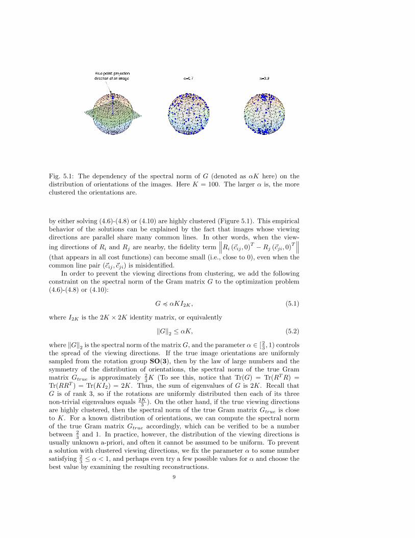
Fig. 5.1: The dependency of the spectral norm of G (denoted as αK here) on thedistribution of orientations of the images. Here K = 100. The larger α is, the moreclustered the orientations are.

by either solving (4.6)-(4.8) or (4.10) are highly clustered (Figure 5.1). This empiricalbehavior of the solutions can be explained by the fact that images whose viewingdirections are parallel share many common lines. In other words, when the view-

ing directions of Ri and Rj are nearby, the fidelity term∥∥∥Ri (~cij , 0)

T −Rj (~cji, 0)T∥∥∥

(that appears in all cost functions) can become small (i.e., close to 0), even when thecommon line pair (~cij ,~cji) is misidentified.

In order to prevent the viewing directions from clustering, we add the followingconstraint on the spectral norm of the Gram matrix G to the optimization problem(4.6)-(4.8) or (4.10):

G 4 αKI2K , (5.1)

where I2K is the 2K × 2K identity matrix, or equivalently

‖G‖2 ≤ αK, (5.2)

where ‖G‖2 is the spectral norm of the matrix G, and the parameter α ∈ [ 23 , 1) controls

the spread of the viewing directions. If the true image orientations are uniformlysampled from the rotation group SO(3), then by the law of large numbers and thesymmetry of the distribution of orientations, the spectral norm of the true Grammatrix Gtrue is approximately 2

3K (To see this, notice that Tr(G) = Tr(RTR) =Tr(RRT ) = Tr(KI2) = 2K. Thus, the sum of eigenvalues of G is 2K. Recall thatG is of rank 3, so if the rotations are uniformly distributed then each of its threenon-trivial eigenvalues equals 2K

3 ). On the other hand, if the true viewing directionsare highly clustered, then the spectral norm of the true Gram matrix Gtrue is closeto K. For a known distribution of orientations, we can compute the spectral normof the true Gram matrix Gtrue accordingly, which can be verified to be a numberbetween 2

3 and 1. In practice, however, the distribution of the viewing directions isusually unknown a-priori, and often it cannot be assumed to be uniform. To preventa solution with clustered viewing directions, we fix the parameter α to some numbersatisfying 2

3 ≤ α < 1, and perhaps even try a few possible values for α and choose thebest value by examining the resulting reconstructions.

9

6. The Alternating Direction Method of Multipliers (ADMM) for SDRswith Spectral Norm Constraint. The application of ADMM to SDP problems wasconsidered in [55]. Here we generalize the application of ADMM to the optimizationproblems considered in previous sections. ADMM is a multiple-splitting algorithmthat minimizes the augmented Lagrangian function in an alternating fashion such thatin each step it minimizes over one block of the variables with all other blocks fixed,and then update the Lagrange multipliers. We apply ADMM to the dual problemssince the linear constraints (6.2) satisfy AA∗ = I which simplifies the computationof subproblems. The strong duality theorem, which is known as Slater’s theorem,guarantees that in the presence of a strictly feasible solution, a primal problem canbe solved by solving its dual problem. To obtain a strictly feasible solution to theprimal problems with the positive semidefinite constraint, the linear constraint (6.2)and the spectral norm constraint (6.3), we can construct a Gram matrix G in (4.3)using rotations sampled from a uniform distribution over the rotation group. There-fore, strong duality holds for the primal problems, and the primal problems can besolved by applying ADMM to their corresponding dual problems.

6.1. The relaxed weighted LS problem. The weighted LS problem after SDR(4.6)-(4.8) can be efficiently solved using SDPLR [4]. However, SDPLR is not suitablefor the problem after the spectral norm constraint on G (5.2) is added to (4.6)-(4.8).This is because the constraint (5.2) can be written as αKI − G < 0, but αKI − Gdoes not have a low rank structure. Moreover, SDP solvers using polynomial-timeprimal-dual interior point methods are designed for small to medium sized problems.Therefore, they are not suitable for our problem. Instead, we devise here a versionof ADMM which takes advantage of the low-rank property of G. After the spectralnorm constraint (5.2) is added, the problem (4.6)-(4.8) becomes

minG<0

− 〈C,G〉 (6.1)

s.t. A (G) = b (6.2)

‖G‖2 ≤ αK (6.3)

where

A (G) =

G11ii

G22ii√

22 G

12ii +

√2

2 G21ii

i=1,2,...,K

, b =

b1ib2ib3i

i=1,2,...,K

, (6.4)

b1i = b2i = 1, b3i = 0 for all i,

Gpqij denotes the (p, q) th element in the 2×2 sub-block Gij , C = W ◦S is a symmetricmatrix and 〈C,G〉 = trace (CG). Following the equality 〈A (G) ,y〉 = 〈G,A∗ (y)〉 for

arbitrary y =

y1i

y2i

y3i

i=1,2,...,K

, the adjoint of the operator A is defined as

A∗ (y) = Y =

(Y 11 Y 12

Y 21 Y 22

),

where for i = 1, 2, . . . ,K

Y 11ii = y1

i , Y22ii = y2

i , and Y 12ii = Y 21

ii = y3i /√

2.

10

It can be verified that AA∗ = I. The dual problem of problem (6.1)-(6.3) is

maxy,X<0

min‖G‖2≤αK

−〈C,G〉 − 〈y,A (G)− b〉 − 〈G,X〉 . (6.5)

By rearranging terms in (6.5), we obtain

maxy,X<0

min‖G‖2≤αK

−〈C +X +A∗ (y) , G〉+ yTb. (6.6)

Using the fact that the dual norm of the spectral norm is the nuclear norm (Propo-sition 2.1 in [34]), we can obtain from (6.6) the dual problem

maxy,X<0

yTb− αK ‖C +X +A∗ (y)‖∗ , (6.7)

where ‖·‖∗ denotes the nuclear norm. Introducing a variable Z = C + X + A∗ (y) ,we obtain from (6.7) that

miny,X<0

− yTb + αK ‖Z‖∗ (6.8)

s.t. Z = C +X +A∗ (y) . (6.9)

Since Z is a symmetric matrix, ‖Z‖∗ is the summation of the absolute values of theeigenvalues of Z. The augmented Lagrangian function of (6.8)-(6.9) is defined as

L (y, Z,X,G) =− yTb + αK ‖Z‖∗ + 〈G,C +X +A∗ (y)− Z〉

+µ

2‖C +X +A∗ (y)− Z‖2F , (6.10)

where µ > 0 is a penalty parameter. Using the augmented Lagrangian function(6.10), we devise an ADMM that minimizes (6.10) with respect to y, Z, X, and G inan alternating fashion, that is, given some initial guess, in each iteration the followingthree subproblems are solved sequentially:

yk+1 = arg minyL(y, Zk, Xk, Gk

), (6.11)

Zk+1 = arg minZL(yk+1, Z,Xk, Gk

), (6.12)

Xk+1 = arg minX<0L(yk+1, Zk+1, X,Gk

), (6.13)

and the Lagrange multiplier G is updated by

Gk+1 = Gk + γµ(C +Xk+1 +A∗

(yk+1

)− Zk+1

), (6.14)

where γ ∈(

0, 1+√

52

)is an appropriately chosen step length.

To solve the subproblem (6.11), we use the first order optimality condition

∇yL(y, Zk, Xk, Gk

)= 0

and the fact that AA∗ = I, and we obtain

yk+1 = −A(C +Xk − Zk

)− 1

µ(A (G)− b) .

11

By rearranging the terms of L(yk+1, Z,Xk, Gk

), it can be verified that the sub-

problem (6.12) is equivalent to

minZ

αK

µ‖Z‖∗ +

1

2

∥∥Z −Bk∥∥2

F,

where Bk = C + Xk + A∗(yk+1

)+ 1

µGk. Let Bk = UΛUT be the spectral de-

composition of the matrix Bk, where Λ = diag (λ) = diag (λ1, . . . , λ2K) . ThenZk+1 = Udiag (z)UT , where z is the optimal solution of the problem

minz

αK

µ‖z‖1 +

1

2‖z− λ‖22 , (6.15)

It can be shown that the unique solution of (6.15) admits a closed form called the soft-thresholding operator, following a terminology introduced by Donoho and Johnstone[8]; it can be written as

zi =

{0, if |λi| ≤ αK/µ(1− α

µ/|λi|)λi, otherwise.

The problem (6.13) can be shown to be equivalent to

minX

∥∥X −Hk∥∥2

F, s.t. X < 0,

where Hk = Zk+1 − C − A∗(yk+1

)− 1

µGk. The solution Xk+1 = V+Σ+V

T+ is the

Euclidean projection of Hk onto the semidefinite cone (section 8.1.1 in [3]), where

V ΣV T =(V+ V−

)( Σ+ 00 Σ−

)(V T+V T−

)is the spectral decomposition of the matrix Hk, and Σ+ and Σ− are the positive andnegative eigenvalues of Hk.

It follows from the update rule (6.14) that

Gk+1 = (1− γ)Gk + γµ

(C +Xk+1 +A∗

(yk+1

)− Zk+1 +

1

µGk)

= (1− γ)Gk + γµ(Xk+1 −Hk

).

6.2. The relaxed LUD problem. Consider the LUD problem after SDR:

minG<0

∑i<j

∥∥~cTij −Gij~cTji∥∥ s.t. A (G) = b, (6.16)

where G, A and b are defined in (4.3) and (6.4) respectively. The ADMM devisedto solve (6.16) is similar to and simpler than the ADMM devised to solve the onewith the spectral norm constraint. We focus on the more difficult problem with thespectral norm constraint. Introducing xij = ~cTij−Gij~cTji and adding the spectral normconstraint ‖G‖2 ≤ αK, we obtain

minxij ,G<0

∑i<j

‖xij‖ s.t. A (G) = b, xij = ~cTij −Gij~cTji, ‖G‖2 ≤ αK. (6.17)

12

The dual problem of problem (6.17) is

maxθij ,y,X<0

minxij ,‖G‖2≤αK

∑i<j

(‖xij‖ −

⟨θij ,xij − ~cTij +Gij~c

Tji

⟩)−〈y,A (G)− b〉−〈G,X〉 .

(6.18)By rearranging terms in (6.18), we obtain

maxθij ,y,X<0

minxij ,‖G‖2≤αK

− 〈Q (θ) +X +A∗ (y) , G〉+ yTb

+∑i<j

(‖xij‖ − 〈θij ,xij〉+

⟨θij ,~c

Tij

⟩), (6.19)

where θ = (θij)i,j=1,...,K , θij =(θ1ij , θ

2ij

)T, ~cij =

(c1ij , c

2ij

),

Q (θ) =1

2

(Q11 (θ) Q12 (θ)Q21 (θ) Q22 (θ)

)and Qpq (θ) =

0 θp12c

q21 · · · θp1Kc

qK1

cq21θp12 0 · · · θp2Kc

qK2

......

. . ....

cqK1θp1K cqK2θ

p2K · · · 0

for p, q = 1, 2. It is easy to verify that for 1 ≤ i < j ≤ K

minxij

(‖xij‖ − 〈θij ,xij〉) =

{0 if ‖θij‖ ≤1

−∞ otherwise.(6.20)

In fact, (6.20) is obtained using the inequality

‖xij‖ − 〈θij ,xij〉 = ‖xij‖ − ‖θij‖ ‖xij‖ 〈θij/ ‖θij‖ ,xij/ ‖xij‖〉≥ ‖xij‖ − ‖θij‖ ‖xij‖ = (1− ‖θij‖) ‖xij‖ , (6.21)

and the inequality in (6.21 ) holds when θij and xij have the same direction. Usingthe fact that the dual norm of the spectral norm is the nuclear norm and the fact in(6.20), we can obtain from (6.19) the dual problem

minθij ,y,X<0

− yTb−∑i<j

⟨θij ,~c

Tij

⟩+ αK ‖Z‖∗ (6.22)

s.t. Z = Q (θ) +X +A∗ (y) , and ‖θij‖ ≤ 1. (6.23)

The augmented Lagrangian function of problem (6.22)-(6.23) is defined as

L (y,θ, Z,X,G) =− yTb + αK ‖Z‖∗ −∑i<j

⟨θij ,~c

Tij

⟩+ 〈G,Q (θ) +X +A∗ (y)− Z〉

+µ

2‖Q (θ) +X +A∗ (y)− Z‖2F , (6.24)

for ‖θij‖ ≤ 1, where µ > 0 is a penalty parameter. Similar to section 6.1, usingthe augmented Lagrangian function (6.24), ADMM is used to minimize (6.24) withrespect to y, θ, Z, X, and G alternatively, that is, given some initial guess, in each

13

iteration the following four subproblems are solved sequentially:

yk+1 = arg minyL(y,θk, Zk, Xk, Gk

), (6.25)

θk+1ij = arg min

‖θij‖≤1L(yk+1,θ, Zk, Xk, Gk

), (6.26)

Zk+1 = arg minZL(yk+1,θk+1, Z,Xk, Gk

), (6.27)

Xk+1 = arg minX<0L(yk+1,θk+1, Zk+1, X,Gk

), (6.28)

and the Lagrange multiplier G is updated by

Gk+1 = Gk + γµ(Q(θk+1

)+Xk+1 +A∗

(yk+1

)− Zk+1

), (6.29)

where γ ∈(

0, 1+√

52

)is an approprately chosen step length. The methods to solve

subproblems (6.25), (6.27) and (6.28) are similar to those used in (6.11), (6.12) and(6.13). To solve subproblem (6.26), we rearrange the terms of L

(yk+1,θ, Zk, Xk, Gk

)and obtain an eqivalent problem

minθij−⟨θij ,~c

Tij

⟩+µ

2‖θij~cji + Φij‖2F , s.t. ‖θij‖ ≤ 1,

where Φ = Xk+A∗(yk+1

)−Zk+ 1

µGk , Φ =

(Φ11 Φ12

Φ21 Φ22

)and Φij =

(Φ11ij Φ12

ij

Φ21ij Φ22

ij

).

Problem (6.29) is further simplified as

minθij

⟨θij , µΦij~c

Tji − ~cTij

⟩+µ

2‖θij‖2 , s.t. ‖θij‖ ≤ 1,

whose solution is

θij =

1µ~cTij − Φij~c

Tij if

∥∥∥ 1µ~cTij − Φij~c

Tij

∥∥∥ ≤ 1,

~cTij−µΦij~cTij

‖~cTij−µΦij~cTij‖otherwise.

The practical issues related to how to take advantage of low-rank assumption of Gin the eigenvalue decomposition performed at each iteration, strategies for adjustingthe penalty parameter µ, the use of a step size γ for updating the primal variableX and termination rules using the in-feasibility measures are discussed in details in[55]. The convergence analysis on ADMM using more than two blocks of variablescan be found in [16]. However, there is one condition of Assumption A (page 5) in [16]that cannot be satisfied for our problem: the condition that the feasible set should bepolyhedral, whereas the SDP cone in our problem is not a polyhedral. To generalizethe convergence analysis in [16] to our problem, we will need to show that the localerror bounds (page 8 - 9 in [16]) hold for the SDP cone. Currently we do not have arigorous convergence proof for ADMM for our problem.

7. The Iterative Reweighted Least Squares (IRLS) Procedure. Since ~cijand ~cji are unit vectors, it is tempting to replace the LUD problem (3.7) with the

14

following semidefinite relaxation:

minG∈R2K×2K

F (G) =∑

i,j=1,2,...,K

√2− 2

∑p,q=1,2

Gpqij Spqij (7.1)

s.t. Gii = I2, i = 1, 2, · · · ,K, (7.2)

G < 0, (7.3)

‖G‖2 ≤ αK (optional), (7.4)

where α is a fixed number between 23 and 1, and the spectral norm constraint on G

(7.4) is added when the solution to the problem (7.1)-(7.3) is a set of highly clusteredrotations. Notice that this relaxed problem is, however, not convex since the objectivefunction (7.1) is concave. We propose to solve (7.1)-(7.3) (possibly with (7.4)) by anvariant of the IRLS procedure [5, 6, 19], which at best converges to a local minimizer.With a good initial guess for G it can be hoped that the global minimizer is obtained.Such an initial guess can be taken as the LS solution.

Algorithm 1 (the IRLS procedure) Solve optimization problem (7.1)-(7.3) (withthe spectral norm constraint on G (7.4) if the input parameter α satisfies 2

3 ≤ α < 1),and then recover the orientations by rounding.

Require: a 2K × 2K common-line matrix S, a regularization parameter ε, a param-eter α and the total number of iterations Niter

w0ij = 1 ∀i, j = 1, · · · ,K;

G0 = 0;for k = 1→ Niter, step size = 1 do

update W by setting wij = wk−1ij ;

if 23 ≤ α < 1, obtain Gk by solving the problem (6.1)-(6.3) using ADMM;

otherwise, obtain Gk by solving (4.6)–(4.8) using SDPLR (with initial guess Gk−1);

rkij =√

2− 2∑p,q=1,2G

pqij S

pqij + ε2;

wkij = 1/rkij ;

the residual rk =∑Ki,j=1 r

kij ;

end forobtain estimated orientations R1, . . . , RK from GNiter using the randomized round-ing procedure in section 4.4.

Before the rounding procedure, the IRLS procedure finds an approximate solutionto the optimization problem (7.1)-(7.3) (possibly with (7.4)) by solving its smoothingversion

minG∈R2K×2K

F (G, ε) =∑

i,j=1,2,...,K

√2− 2

∑p,q=1,2

Gpqij Spqij + ε2 (7.5)

s.t. Gii = I2, i = 1, 2, · · · ,K, (7.6)

G < 0, (7.7)

‖G‖2 ≤ αK (optional). (7.8)

where ε > 0 is a small number. The solution to the smoothing version is close tothe solution to the original problem. In fact, let G∗ε = arg minF (G, ε) and G∗ =

15

arg minF (G), then we shall verify that

|F (G∗ε )− F (G∗)| ≤ 4K2ε. (7.9)

Using the fact that

0 ≤ F (G, ε)− F (G) < 4K2ε,

we obtain

(F (G∗, ε)− F (G∗ε , ε)) + (F (G∗ε )− F (G∗))

=(F (G∗, ε)− F (G∗))− (F (G∗ε , ε)− F (G∗ε ))≤4K2ε.

Since F (G∗, ε)− F (G∗ε , ε) ≥ 0 and F (G∗ε )− F (G∗) ≥ 0, the inequality (7.9) holds.

In each iteration, the IRLS procedure solves the problem

Gk+1 = arg minG<0

∑i 6=j

wkij(2− 2 〈Gij , Sij〉+ ε2

)s.t. A(G) = b, (optional: ‖G‖2 ≤ αK)

(7.10)on the (k + 1)th iteration, where w0

ij = 1, and

wkij = 1/√

2− 2⟨Gkij , Sij

⟩+ ε2, ∀k > 0.

In other words, in each iteration, more emphasis is given to detected common-linesthat are better explained by the current estimate Gk of the Gram matrix. Theinclusion of the regularization parameter ε ensures that no single detected common-line can gain undue influence when solving

Gk+1 = arg maxG<0

⟨W k ◦ S,G

⟩s.t. A(G) = b (optional: ‖G‖2 ≤ αK). (7.11)

We repeat the process until the residual sequence {rk} has converged, or the maximumnumber of iterations has been reached. We shall verify that the value of the costfunction is non-increasing, and that every cluster point of the sequence of IRLS is astationary point of (7.5) - (7.7) in the following lemma and theorem, for the problemwithout the spectral norm constraint on G. The arguments can be generalized to thecase with the spectral norm constraint. The proof of Theorem 7.2 follows the methodof proof for Theorem 3 in the paper [25] by Mohan et. al..

Lemma 7.1. The value of the cost function sequence is monotonically non-increasing, i.e.,

F (Gk+1, ε) ≤ F (Gk, ε). (7.12)

where{Gk}

is the sequence generated by the IRLS procedure of Algorithm 1.

Proof. Since Gk is the solution of (7.11), there exists yk ∈ R2K and Xk ∈ R2K×2K

such that

−A∗(yk) +Xk +W k−1 ◦ S = 0, A(Gk)− b = 0, (7.13)

Gk < 0, Xk < 0,⟨Gk, Xk

⟩= 0. (7.14)

16

Hence we have

0 = −(yk)T (A(Gk)− b) + (yk+1)T (A(Gk+1)− b)

= (yk+1 − yk)T (A(Gk)− b) +⟨A∗(yk+1), Gk+1 −Gk

⟩=⟨Xk+1 +W k ◦ S,Gk+1 −Gk

⟩≤⟨W k ◦ S,Gk+1 −Gk

⟩(7.15)

=1

2

∑i 6=j

(−βkij

(2− 2

⟨Gk+1ij , Sij

⟩+ ε2

)+ βkij

(2− 2

⟨Gkij , Sij

⟩+ ε2

))

=1

2

∑i 6=j

− 2− 2⟨Gk+1ij , Sij

⟩+ ε2√

2− 2⟨Gkij , Sij

⟩+ ε2

+√

2− 2⟨Gkij , Sij

⟩+ ε2

, (7.16)

where the third equality uses (7.13), and the inequality (7.15) uses (7.14). From (7.16)we obtain

F (Gk, ε)2 =

∑i 6=j

√2− 2

⟨Gkij , Sij

⟩+ ε2

2

≥

∑i 6=j

√2− 2

⟨Gkij , Sij

⟩+ ε2

∑i 6=j

2− 2⟨Gk+1ij , Sij

⟩+ ε2√

2− 2⟨Gkij , Sij

⟩+ ε2

≥

∑i 6=j

√2− 2

⟨Gk+1ij , Sij

⟩+ ε2

2

= F (Gk+1, ε)2, (7.17)

where the last inequality uses Cauchy-Schwarz inequality and the equality holds ifand only if √

2− 2⟨Gk+1ij , Sij

⟩+ ε2√

2− 2⟨Gkij , Sij

⟩+ ε2

= c for all i 6= j, (7.18)

where c is a constant. Thus (7.12) is confirmed.Theorem 7.2. The sequence of iterates

{Gk}

of IRLS is bounded, and everycluster point of the sequence is a stationary point of (7.5) - (7.7).

Proof. Since trace(Gk) = 2K and Gk < 0, the sequence{Gk}

is bounded. Itfollows that W k and trace((W k ◦ S)Gk+1) are bounded. Using the strong duality ofSDP, we conclude that bTyk+1 =trace((W k ◦ S)Gk+1) is bounded. In addition, fromthe KKT conditions (7.13) - (7.14) we obtain −A∗(yk+1) + W k ◦ S < 0. Using thedefinition of A∗ and S, the property of semi-definite matrices and the fact that W k

is bounded, it can be verified that yk is bounded. Using (7.13) again, we obtain∥∥Xk∥∥ =

∥∥A∗(yk)−W k−1 ◦ S∥∥ ≤ ∥∥A∗(yk)

∥∥+∥∥W k−1 ◦ S

∥∥ ,which implies that Xk is bounded.

We now show that every cluster point of{Gk}

is a stationary point of (7.5) -

(7.7). Suppose to the contrary and let G be a cluster point of{Gk}

that is nota stationary point. By the definition of cluster point, there exists a subsequence

17

{Gki ,W ki , Xki ,yki

}of{Gk,W k, Xk,yk

}converging to

(G, W , X, y

). By passing to

a further subsequence if necessary, we can assume that{Gki+1,W ki+1, Xki+1,yki+1

}is also convergent and we denote its limit by

(G, W , X, y

). Gki+1 is defined as (7.10)

or (7.11) and satisfies the KKT conditions (7.13) - (7.14). Passing to limits, we seethat

−A∗(y) + X + W ◦ S = 0,A(G)− b = 0,

G < 0, X < 0,⟨G, X

⟩= 0.

Thus we conclude that G is a maximizer of the following convex optimization problem,

maxG<0

⟨W ◦ S,G

⟩s.t. A(G) = b.

Next, by assumption, G is not a stationary point of (7.5) - (7.7). This implies that G

is not a maximizer of the problem above and thus⟨W ◦ S, G

⟩>⟨W ◦ S, G

⟩. From

this last relation and (7.17) - (7.18) it follows that

F (G, ε) < F (G, ε). (7.19)

Otherwise if F (G, ε) = F (G, ε), then⟨Gij , Sij

⟩=⟨Gij , Sij

⟩due to (7.17) - (7.18),

and thus we would obtain⟨W ◦ S, G

⟩=⟨W ◦ S, G

⟩which is a contradiction.

On the other hand, it follows from Lemma 7.1 that the sequence{F (Gk, ε)

}converges. Thus we have that

limF (Gk, ε) = limF (Gki , ε) = F (G, ε) = limF (Gki+1, ε) = F (G, ε)

which contradicts (7.19). Hence, every cluster point of the sequence is a stationarypoint of (7.5) - (7.7).

In addition, using Holder’s inequality, the analysis can be generalized to thereweighted approach to solve

minG<0

∑i 6=j

(2− 2 〈Gij , Sij〉)p2 s.t. A(G) = b, (optional: ‖G‖2 ≤ αK) (7.20)

where 0 < p < 1. Convergence analysis of IRLS for different applications with p < 1can be found in [6, 19]. The problem (7.20) is a SDR of the problem

minR1,...,RK∈SO(3)

∑i 6=j

∥∥∥Ri (~cij , 0)T −Rj (~cji, 0)

T∥∥∥p . (7.21)

The smaller p is, the more penalty the outliers in the detected common-lines receive.

8. Numerical results. All numerical experiments were performed on a machinewith 2 Intel(R) Xeon(R) CPUs X5570, each with 4 cores, running at 2.93 GHz. Inall the experiments, the polar Fourier transform of images for common-line detectionhad radial resolution nr = 100 and angular resolution nθ = 360. The number ofiterations was set to be Niter = 10 in all IRLS procedures. The reconstruction fromthe images with estimated orientations used the Fourier based 3D reconstruction

18

Clean SNR = 1/16 SNR = 1/32 SNR = 1/64

Fig. 8.1: The first column shows three clean images of size 129× 129 pixels generatedfrom a 50S ribosomal subunit volume with different orientations. The other threecolumns show three noisy images corresponding to those in the first column withSNR= 1/16, 1/32 and 1/64, respectively.

package FIRM3 [52]. The reconstructed volumes are shown in Figure 8.2 and 8.5using the visualization system Chimera [32].

To evaluate the accuracy or the resolution of the reconstructions, we used the 3DFourier Shell Correlation (FSC) [36]. FSC measures the normalized cross-correlationcoefficient between two 3D volumes over corresponding spherical shells in Fourierspace, i.e.,

FSC (i) =

∑j∈Shelli F (V1) (j) · F (V2) (j)√∑

j∈Shelli |F (V1) (j)|2 ·∑

j∈Shelli |F (V2) (j)|2, (8.1)

where F (V1) and F (V2) are the Fourier transforms of volume V1 and volume V2

respectively, the spatial frequency i ranges from 1 to N/2−1 times the unit frequency1/(N · pixel size), N is the size of a volume, and Shelli := {j : 0.5 + (i − 1) + ε ≤‖j‖ < 0.5 + i + ε} where ε =1e-4. In this form, the FSC takes two 3D volumes andconverts them into a 1D array. In Section 8.2, we used the FSC 0.143 cutoff criterion[2, 37] to determine the resolutions of the ab-initio models and the refined models.

8.1. Experiments on simulated images. We simulated 500 centered imagesof size 129 × 129 pixels with pixel size 2.4A of the 50S ribosomal subunit (the topvolume in Figure 8.2), where the orientations of the images were sampled from theuniform distribution over SO(3). White Gaussian noise was added to the clean imagesto generate noisy images with SNR= 1/16, 1/32 and 1/64 respectively (Figure 8.1).

3The FIRM package is available at https://web.math.princeton.edu/~lanhuiw/software.html.

19

Fig. 8.2: The clean volume (top), the reconstructed volumes and the MSEs (8.2) of theestimated rotations. From 2nd to 4th row, no spectral norm constraint was used (i.e.,α = N/A) for all algorithms. The last 4 rows are all results of very noisy images withSNR = 1/64, where the result using the IRLS procedure without α is not availabledue to the highly clustered estimated projection directions, and the result from theIRLS procedure with α = 0.67 for the spectral norm constraint is best.

20

Common-line pairs that were detected with an error smaller than 10◦ were consideredto be correct. The common-line detection rates were 64%, 44% and 23% for imageswith SNR=1/16, 1/32 and 1/64 respectively (Figure 3.1).

To measure the accuracy of the estimated orientations, we defined the meansquared error (MSE) of the estimated rotation matrices R1, . . . , RK as

MSE =1

K

K∑i=1

∥∥∥Ri − ORi∥∥∥2

, (8.2)

where O is the optimal solution to the registration problem between the two sets of

rotations {R1, . . . , RK} and{R1, . . . , RK

}in the sense of minimizing the MSE. As

shown in [41], there is a simple procedure to obtain both O and the MSE from the

singular value decomposition of the matrix 1K

∑Ki=1 RiR

Ti .

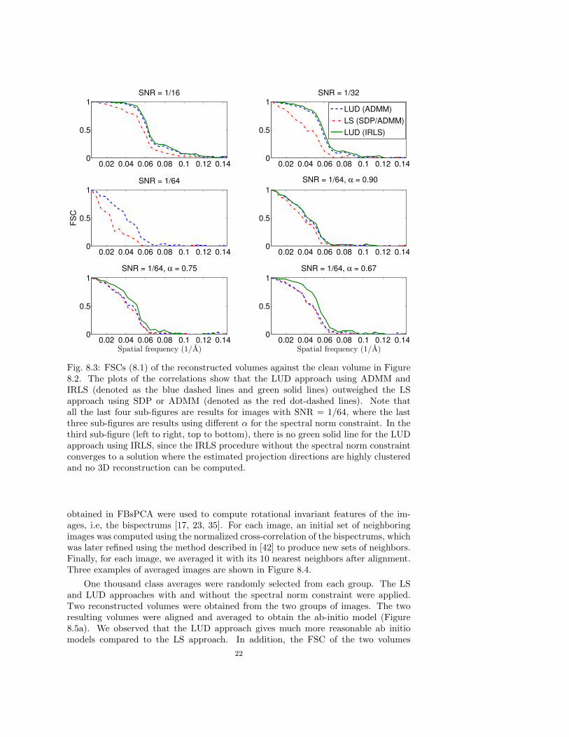
We applied the LS approach using SDP and ADMM, and the LUD approach usingADMM and IRLS to estimate the images’ orientations, then computed the MSEs ofthe estimated rotation matrices, and lastly reconstructed the volume (Figure 8.2).In order to measure the accuracy of the reconstructed volumes, we measured eachvolume’s FSC (8.1) (Figure 8.3) against the clean 50S ribosomal subunit volume, thatis, in our measurement V1 was the reconstructed volume, and V2 was the “groundtruth” volume.

When SNR= 1/16 and 1/32, the common-line detection rate was relatively high(64% and 44%), the algorithms without the spectral norm constraint onG were enoughto make a good estimation. The LUD approach using ADMM and IRLS outweighedthe LS approach in terms of accuracy measured by MSE and FSC (Figure 8.2-8.3).Note that the LS approach using SDP failed when SNR = 1 /32, while the LUDapproach using either ADMM or IRLS succeeded. When SNR=1/64, the common-linedetection rate was relatively small (23%), and most of the detected common-lines wereoutliers (Figure 3.1), the algorithms without spectral norm constraint ‖G‖2 ≤ αKdid not work. Especially, the viewing directions of images estimated by the IRLSprocedures without ‖G‖2 ≤ αK converged to two clusters around two antipodaldirections, yielding no 3D reconstruction. The LUD approach using ADMM failedin this case, however, the IRLS procedure with an appropriate regularization on thespectral norm (i.e., α = 0.67 since the true rotations were uniformly sampled overSO(3)) gave the best reconstruction.

8.2. Experiments on a real dataset. A set of micro-graphs of E. coli 50Sribosomal subunits was provided by Dr. M. van Heel. These micro-graphs wereacquired by a Philips CM20 at defocus values between 1.37 and 2.06 µm, and they werescanned at 3.36 A/pixel. The particles (particularly E. coli 50S ribosomal subunits)were picked using the automated particle picking algorithm in EMAN Boxer [20].Then using the IMAGIC software package ([45, 51]), the 27,121 particle images of size90×90 pixels were phase-flipped to remove the phase-reversals in the CTF, bandpassfiltered at 1/150 and 1/8.4 A, normalized by their variances, and then translationallyaligned with the rotationally-averaged total sum. The particle images were randomlydivided into 2 disjoint groups of equal number of images. The following steps wereperformed to each group separately.

The images were rotationally aligned and averaged to produce class averages ofbetter quality, following the procedure detailed in [58]. For each group, the imageswere denoised and compressed using Fourier-Bessel based principal component anal-ysis (FBsPCA) [57]. Then, triple products of Fourier-Bessel expansion coefficients

21

0.02 0.04 0.06 0.08 0.1 0.12 0.140

0.5

1SNR = 1/16

0.02 0.04 0.06 0.08 0.1 0.12 0.140

0.5

1SNR = 1/32

0.02 0.04 0.06 0.08 0.1 0.12 0.140

0.5

1

FS

C

SNR = 1/64

0.02 0.04 0.06 0.08 0.1 0.12 0.140

0.5

1

SNR = 1/64, α = 0.90

0.02 0.04 0.06 0.08 0.1 0.12 0.140

0.5

1

Spatial frequency (1/A)

SNR = 1/64, α = 0.75

0.02 0.04 0.06 0.08 0.1 0.12 0.140

0.5

1

Spatial frequency (1/A)

SNR = 1/64, α = 0.67

LUD (ADMM)

LS (SDP/ADMM)

LUD (IRLS)

Fig. 8.3: FSCs (8.1) of the reconstructed volumes against the clean volume in Figure8.2. The plots of the correlations show that the LUD approach using ADMM andIRLS (denoted as the blue dashed lines and green solid lines) outweighed the LSapproach using SDP or ADMM (denoted as the red dot-dashed lines). Note thatall the last four sub-figures are results for images with SNR = 1/64, where the lastthree sub-figures are results using different α for the spectral norm constraint. In thethird sub-figure (left to right, top to bottom), there is no green solid line for the LUDapproach using IRLS, since the IRLS procedure without the spectral norm constraintconverges to a solution where the estimated projection directions are highly clusteredand no 3D reconstruction can be computed.

obtained in FBsPCA were used to compute rotational invariant features of the im-ages, i.e, the bispectrums [17, 23, 35]. For each image, an initial set of neighboringimages was computed using the normalized cross-correlation of the bispectrums, whichwas later refined using the method described in [42] to produce new sets of neighbors.Finally, for each image, we averaged it with its 10 nearest neighbors after alignment.Three examples of averaged images are shown in Figure 8.4.

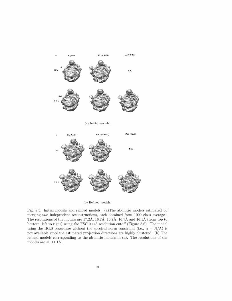
One thousand class averages were randomly selected from each group. The LSand LUD approaches with and without the spectral norm constraint were applied.Two reconstructed volumes were obtained from the two groups of images. The tworesulting volumes were aligned and averaged to obtain the ab-initio model (Figure8.5a). We observed that the LUD approach gives much more reasonable ab initiomodels compared to the LS approach. In addition, the FSC of the two volumes

22

Raw image Average image1st Neighbor 2nd Neighbor

Fig. 8.4: Noise reduction by image averaging. Three raw ribosomal images are shownin the first column. Their closest two neighbours (i.e., raw images having similarorientations after alignments) are shown in the second and third columns. The averageimages shown in the last column were obtained by averaging over 10 neighbours ofeach raw image.

was computed to estimate the resolution of the ab-initio model (Figure 8.6). Amongall the ab-initio models, the one obtained by LS is at the lowest resolution 17.2A,while the one obtained by LUD through IRLS procedure is the highest resolution16.1A. Notice that the FSC measures the variance error, but not the bias error of theab-initio model. We also notice that the viewing directions of images estimated bythe IRLS procedures without the spectral norm constraint converged to two clustersaround two antipodal directions, resulting in no 3D reconstruction. Moreover, for thisdataset, adding the spectral norm constraint on G with α = 0.85 did not improve theaccuracy of the result, although this helped with regularizing the convergence in theIRLS procedure.

The two resulting volumes were then iteratively refined using 10,000 raw imagesin each group. In each refinement iteration, 2,000 template images were generatedby projecting the 3D model from the previous iteration, then the orientations of theraw images were estimated using reference-template matching, and finally a new 3Dmodel was reconstructed from the 10,000 raw images with highest correlation with thereference images. Each refinement iteration took about 4 hours. Therefore, a goodab-initio model should be able to accelerate the refinement process by reducing thetotal number of refinement iterations. The FSC plots in Figure 8.6a - 8.6e show theconvergence of the refinement process using different ab-initio models. We observedthat all the refined models are at the resolution 11.1A. However, the worst ab-initio

23

model obtained by LS needed 7 iterations (about 28 hours) for convergence (Figure8.6a), while the best ab-initio model obtained by LUD needed 3 iterations (about 12hours) for convergence (Figure 8.6b and Figure 8.6d). Figure 8.6f uses FSC plots tocompare the refined models. We observed that the refined models in Figure 8.6b -8.6e were consistent to each other, while the refined model obtained by LS in Figure8.6a was slightly different from others.

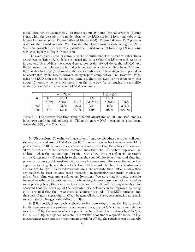
The average cost time for computing the ab-initio models in these two subsectionsare shown in Table (8.1). It is not surprising to see that the LS approach was thefastest and that adding the spectral norm constraint slowed down the ADMM andIRLS procedures. The reason is that a large portion of the cost time in ADMM andIRLS is due to the projections onto the semidefinite cone. These steps are expected tobe accelerated by the recent advance on eigenspace computation [56]. However, whenusing the LUD approach for the real data set, the time saved in the refinement wasabout 16 hours, which is much more than the time cost for computing the ab-initiomodels (about 0.5 - 1 hour when ADMM was used).

α = N/A 23 ≤ α ≤ 1

K LS LUD LS LUD(SDP) ADMM IRLS (ADMM) ADMM IRLS

500 7s 266s 469s 78s 454s 3353s1000 31s 1864s 3913s 619s 1928s 20918s

Table 8.1: The average cost time using different algorithms on 500 and 1000 imagesin the two experimental subsections. The notation α = N/A means no spectral normconstraint ‖G‖2 ≤ αK is used.

9. Discussion. To estimate image orientations, we introduced a robust self con-sistency error and used ADMM or the IRLS procedure to solve the associated LUDproblem after SDR. Numerical experiments demonstrate that the solution is less sen-sitive to outliers in the detected common-lines than the LS method approach. Inaddition, when the common-line detection rate is low, the spectral norm constrainton the Gram matrix G can help to tighten the semidefinite relaxation, and thus im-proves the accuracy of the estimated rotations in some cases. Moreover, the numericalexperiments using the real data set (Section 8.2) demonstrate that the ab-initio mod-els resulted by the LUD based methods are more accurate than initial models thatare resulted by least squares based methods. In particular, our initial models re-quires fewer time-consuming refinement iterations. We note that it is also possibleto consider other self consistency errors involving the unsquared deviations raised tosome power p (e.g., the cases p = 1, 2 correspond to LUD and LS, respectively). Weobserved that the accuracy of the estimated orientations can be improved by usingp < 1 provided that the initial guess is “sufficiently good”. The LUD approach andthe spectral norm constraint on G can be generalized to the synchronization approachto estimate the images’ orientations in [39].

In [54], the LUD approach is shown to be more robust than the LS approachfor the synchronization problem over the rotation group SO(d). Given some relativerotations RTi Rj , the synchronization problem is to estimate the rotations Ri ∈ SO(d),i = 1, . . . ,K up to a global rotation. It is verified that under a specific model of themeasurement noise and the measurement graph for RTi Rj , the rotations can be exactly

24

and stably recovered using LUD, exhibiting a phase transition behavior in terms of theproportion of noisy measurements. The problem of orientation determination usingcommon-lines between cryo-EM images is similar to the synchronization problem. Thedifference is that the pairwise information given by the relative rotation RTi Rj is full,while that given by the common-lines ~cTji~cij is partial. Moreover, the measurementnoise of each detected common-line ~cij depends on image i and j, and thus it cannotbe simply modeled, which brings the difficulties in verifying the conditions for theexact and stable orientation determination we observed.

10. Acknowledgements. The authors would like to thank Zhizhen Zhao forproducing class averages from the experimental ribosomal images. The work of L.Wang and A. Singer was partially supported by Award Number FA9550-12-1-0317from AFOSR, by Award Number R01GM090200 from the NIGMS, by the Alfred P.Sloan Foundation, and by the Simons Foundation. The work of Z. Wen was partiallysupported by NSFC grant 11101274.

References.[1] K. S. Arun, T. S. Huang, and S. D. Blostein. Least-Squares Fitting of Two 3-D

Point Sets. IEEE Trans. Pattern Anal. Mach. Intell., 9(5):698–700, May 1987.[2] X. Bai, I. S. Fernandez, G. McMullan, and S. HW Scheres. Ribosome structures

to near-atomic resolution from thirty thousand cryo-EM particles. eLife Sciences,2, 2013.

[3] S. Boyd and L. Vandenberghe. Convex Optimization. Cambridge UniversityPress, New York, NY, USA, 2004.

[4] S. Burer and R. D. C. Monteiro. A Nonlinear Programming Algorithm for SolvingSemidefinite Programs via Low-rank Factorization. Mathematical Programming(series B), 95:2003, 2001.

[5] Emmanuel J. Candes, Michael B. Wakin, and Stephen P. Boyd. Enhancing spar-sity by reweighted `1 minimization. Journal of Fourier Analysis and Applications,14:877–905, 2008.

[6] I. Daubechies, R. DeVore, M. Fornasier, and C. S. Gunturk. Iterativelyreweighted least squares minimization for sparse recovery. Communications onPure and Applied Mathematics, 63(1):1–38, 2010.

[7] E. de Klerk. Aspects of Semidefinite Programming: Interior Point Algorithmsand Selected Applications. Applied Optimization. Springer, 2002.

[8] D. L. Donoho and I. M. Johnstone. Adapting to Unknown Smoothnessvia Wavelet Shrinkage. Journal of the American Statistical Association,90(432):1200+, December 1995.

[9] A. Dutt and V. Rokhlin. Fast Fourier Transforms for Nonequispaced Data.SIAM Journal on Scientific Computing, 14(6):1368–1393, 1993.

[10] N. A. Farrow and F. P. Ottensmeyer. A posteriori determination of relativeprojection directions of arbitrarily oriented macromolecules. J. Opt. Soc. Am.A, 9(10):1749–1760, Oct 1992.

[11] J. A. Fessler and B. P. Sutton. Nonuniform fast Fourier transforms using min-max interpolation. IEEE Transactions on Signal Processing, 51(2):560 – 574,2003.

[12] J. Frank. Three Dimensional Electron Microscopy of Macromolecular Assemblies.Academic Press, Inc., 1996.

[13] J. Frank. Cryo-electron microscopy as an investigative tool: the ribosome as anexample. BioEssays, 23(8):725–732, 2001.

[14] M. X. Goemans and D.P. Williamson. Improved Approximation Algorithms

25

for Maximum Cut and Satisfiability Problems Using Semidefinite Programming.Journal of the ACM, 42:1115–1145, 1995.

[15] L. Greengard and J. Lee. Accelerating the Nonuniform Fast Fourier Transform.SIAM Review, 46(3):443–454, 2004.

[16] M. Hong and Z.-Q. Luo. On the Linear Convergence of the Alternating DirectionMethod of Multipliers. ArXiv e-prints, August 2012.

[17] R. I. Kondor. A complete set of rotationally and translationally invariant featuresfor images. CoRR, abs/cs/0701127, 2007.

[18] L. Lebart, A. Morineau, and K. M. Warwick. Multivariate descriptive statisti-cal analysis: correspondence analysis and related techniques for large matrices.Wiley series in probability and mathematical statistics: Applied probability andstatistics. Wiley, 1984.

[19] G. Lerman, M. McCoy, J. A. Tropp, and T. Zhang. Robust computation of linearmodels, or How to find a needle in a haystack. arXiv:1202.4044v1 [cs.IT], 2012.

[20] S.J. Ludtke, P. R. Baldwin, and W. Chiu. EMAN: Semiautomated Software forHigh-Resolution Single-Particle Reconstructions. Journal of Structural Biology,128(1):82 – 97, 1999.

[21] Z. Luo, W. Ma, A. So, Y. Ye, and S. Zhang. Semidefinite Relaxation of QuadraticOptimization Problems. IEEE Signal Processing Magazine, 27(3):20–34, may2010.

[22] S.P. Mallick, S. Agarwal, D.J. Kriegman, S.J. Belongie, B. Carragher, andC.S. Potter. Structure and view estimation for tomographic reconstruction: Abayesian approach. In Computer Vision and Pattern Recognition, 2006 IEEEComputer Society Conference on, volume 2, pages 2253–2260, 2006.

[23] R. Marabini and J. M. Carazo. On a new computationally fast image invariantbased on bispectral projections. Pattern Recogn. Lett., 17(9):959–967, 1996.

[24] F. Mezzadri. How to generate random matrices from the classical compact groups.Notices of the AMS, 54:592–604, 2007.

[25] K. Mohan and M. Fazel. Iterative reweighted algorithms for matrix rank mini-mization. Journal of Machine Learning Research, 13:3441–3473, 2012.

[26] F. Natterer. The Mathematics of Computerized Tomography. Classics in Appl.Math. 32. SIAM, Philadelphia, 2001.

[27] H. Nyquist. Least orthogonal absolute deviations. Computational Statistics &Data Analysis, 6(4):361–367, June 1988.

[28] P. Penczek, R. Grassucci, and J. Frank. The ribosome at improved resolution:New techniques for merging and orientation refinement in 3D cryo-electron mi-croscopy of biological particles. Ultramicroscopy, 53(3):251 – 270, 1994.

[29] P. Penczek, M. Radermacher, and J. Frank. Three-dimensional reconstruction ofsingle particles embedded in ice. Ultramicroscopy, 40(1):33–53, 1992.

[30] P. A. Penczek, R. A. Grassucci, and J. Frank. The ribosome at improved resolu-tion: New techniques for merging and orientation refinement in 3d cryo-electronmicroscopy of biological particles. Ultramicroscopy, 53(3):251 – 270, 1994.

[31] P. A. Penczek, J. Zhu, and J. Frank. A common-lines based method for determin-ing orientations for N > 3 particle projections simultaneously. Ultramicroscopy,63(3-4):205 – 218, 1996.

[32] E. F. Pettersen, T. D. Goddard, C. C. Huang, G. S. Couch, D. M. Greenblatt,E. C. Meng, and T. E. Ferrin. UCSF Chimera - A visualization system forexploratory research and analysis. Journal of Computational Chemistry, 25:1605–1612, 2004.

26

[33] M. Radermacher, T. Wagenknecht, A. Verschoor, and J. Frank. A new 3-D recon-struction scheme applied to the 50S ribosomal subunit of E. coli. Ultramicroscopy,141:RP1–2, 1986.

[34] B. Recht, M. Fazel, and P. A. Parrilo. Guaranteed Minimum-Rank Solutions ofLinear Matrix Equations via Nuclear Norm Minimization. SIAM Rev., 52(3):471–501, August 2010.

[35] B. M. Sadler and G. B. Giannakis. Shift- and rotation-invariant object recon-struction using the bispectrum. J. Opt. Soc. Am. A, 9(1):57–69, Jan 1992.

[36] W. O. Saxton and W. Baumeister. The correlation averaging of a regularlyarranged bacterial cell envelope protein. Journal of Microscopy, 127(2):127–138,1982.

[37] S. HW Scheres and S. Chen. Prevention of overfitting in cryo-EM structuredetermination. Nat Meth, 9:853–854, 2012.

[38] I. I. Serysheva, E. V. Orlova, W. Chiu, M. B. Sherman, S. L. Hamilton, andM. van Heel. Electron cryomicroscopy and angular reconstitution used to visu-alize the skeletal muscle calcium release channel. Nat Struct Mol Biol, 2:18–24,1995.

[39] Y. Shkolnisky and A. Singer. Viewing direction estimation in cryo-EM usingsynchronization. SIAM Journal on Imaging Sciences, 5(3):1088–1110, 2012.

[40] A. Singer, R. R. Coifman, F. J. Sigworth, D. W. Chester, and Y. Shkolnisky.Detecting consistent common lines in cryo-EM by voting. Journal of StructuralBiology, 169(3):312–322, 2010.

[41] A. Singer and Y. Shkolnisky. Three-Dimensional Structure Determination fromCommon Lines in Cryo-EM by Eigenvectors and Semidefinite Programming.SIAM Journal on Imaging Sciences, 4(2):543–572, 2011.

[42] A. Singer, Z. Zhao, Y. Shkolnisky, and R. Hadani. Viewing Angle Classification ofCryo-Electron Microscopy Images Using Eigenvectors. SIAM Journal on ImagingSciences, 4(2):723–759, 2011.

[43] A. So, J. Zhang, and Y. Ye. On approximating complex quadratic optimizationproblems via semidefinite programming relaxations. Math. Program., 110(1):93–110, March 2007.

[44] H. Spath and G. A. Watson. On orthogonal linear approximation. Numer. Math.,51(5):531–543, October 1987.

[45] H. Stark, M. V. Rodnina, H. Wieden, F. Zemlin, W. Wintermeyer, and M. vanHeel. Ribosome interactions of aminoacyl-tRNA and elongation factor Tu in thecodon-recognition complex. Nat Struct Mol Biol, 9:849–854, 2002.

[46] B. Vainshtein and A. Goncharov. Determination of the spatial orientation ofarbitrarily arranged identical particles of an unknown structure from their pro-jections. In Proc. llth Intern. Congr. on Elec. Mirco., pages 459–460, 1986.

[47] M. van Heel. Multivariate statistical classification of noisy images (randomlyoriented biological macromolecules). Ultramicroscopy, 13(1-2):165 – 183, 1984.

[48] M. van Heel. Angular reconstitution: A posteriori assignment of projection di-rections for 3D reconstruction. Ultramicroscopy, 21(2):111 – 123, 1987.

[49] M. van Heel and J. Frank. Use of multivariates statistics in analysing the imagesof biological macromolecules. Ultramicroscopy, 6(1):187 – 194, 1981.

[50] M. van Heel, B. Gowen, R. Matadeen, E. V. Orlova, R. Finn, T. Pape, D. Cohen,H. Stark, R. Schmidt, M. Schatz, and A. Patwardhan. Single-particle electroncryo-microscopy: towards atomic resolution. Quarterly Reviews of Biophysics,33(04):307–369, 2000.

27

[51] M. van Heel, G. Harauz, E. V. Orlova, R. Schmidt, and M. Schatz. A newgeneration of the imagic image processing system. Journal of Structural Biology,116(1):17 – 24, 1996.

[52] C. Vonesch, Lanhui Wang, Y. Shkolnisky, and A. Singer. Fast wavelet-basedsingle-particle reconstruction in Cryo-EM. In Biomedical Imaging: From Nanoto Macro, 2011 IEEE International Symposium on, pages 1950 –1953, 2011.

[53] L. Wang and F. J. Sigworth. Cryo-EM and single particles. Physiology(Bethesda), 21:13–18, 2006.

[54] L. Wang and A. Singer. Exact and stable recovery of rotations for robust synchro-nization, 2012. submitted. Also availabe at http://arxiv.org/abs/1211.2441.

[55] Z. Wen, D. Goldfarb, and W. Yin. Alternating direction augmented Lagrangianmethods for semidefinite programming. Mathematical Programming Computa-tion, 2:203–230, 2010.

[56] Z. Wen, C. Yang, X. Liu, and Y. Zhang. Trace-Penalty Minimization for Large-scale Eigenspace Computation. Optimization Online, 2013.

[57] Z. Zhao and A. Singer. Fourier-Bessel rotational invariant eigenimages, 2012.Submitted. Also available at http://arxiv.org/abs/1211.1968.

[58] Z. Zhao and A. Singer. Rotationally Invariant Image Representation for ViewingAngle Classification, 2013. In preparation.

[59] Z. Zhu, A. So, and Y. Ye. Universal Rigidity and Edge Sparsification for Sensor-Network Localization. SIAM Journal on Optimization, 20(6):3059–3081, 2010.

Appendix. Exact recovery of the Gram matrix G from correct common-lines. Here we prove that if the detected common-lines ~cji (defined in (3.1)) are allcorrect and at least three images have linearly independent projection directions (i.e.,the viewing directions of the three images are not on the same great circle on thesphere shown in Figure 5.1), then the Gram matrix G obtained by solving the LSproblem (4.6)-(4.8) or the LUD problem (4.10) is uniquely the one defined in (4.3).To verify the uniqueness of the solution G, it is enough to show rank(G)= 3 due to theSDP solution uniqueness theorem (page 36-39 in [7], [59]). Without loss of generality,we consider the SDP for the LS approach when applied on three images (i.e., K = 3and wij = 1 in the problem (4.6) - (4.8)):

maxG6×6<0

∑i,j=1,2,3

⟨Gij ,~c

Tji~cij

⟩s.t. Gii = I2,

Since the solution G is positive semidefinite, we can decompose G as

G =

u1T

1

u2T

1

u1T

2

u2T

2

u1T

3

u2T

3

(

u11 u2

1 u12 u2

2 u13 u2

3

),

where upi , p = 1, 2 and i = 1, 2, 3 are column vectors. We will show rank(G)= 3, i.e.,any four vectors among

{u1

1,u21,u

12,u

22,u

13,u

23

}span a space with dimensionality at

most 3.Define arrays ui as

ui = (u1i ,u

2i ),

28

then the inner product⟨Gij ,~c

Tji~cij

⟩=⟨uTi uj ,~c

Tji~cij

⟩= 〈~cjiui,~cijuj〉=⟨c1jiu

1i + c2jiu

2i , c

1iju

1j + c2iju

2j

⟩≤ 1,

where the last inequality follows the Cauchy-Schwarz inequality and the facts thatall ~cij are unit vectors, u1

i and u2i are unit vectors and orthogonal to each other due

to the constraint Gii = I2, and thus all c1iju1j + c2iju

2j are unit vectors on the Fourier

slices of the images. The equality holds if and only if

c1jiu1i + c2jiu

2i = c1iju

1j + c2iju

2j . (A.1)

Thus when the maximum is achieved, due to (A.1) and the fact that the projection di-rections of the images are linearly independent, dim(span{u1

i ,u2i }∩span{u1

j ,u2j})= 1

and thus dim(span{u1i ,u

2i ,u

1j ,u

2j})= 3. Therefore, without loss of generality, we

only have to show that dim(span{u11,u

12,u

13,u

23})≤ 3. Using (A.1), assume that

span{u11,u

21}∩span{u1

3,u23}=span{v1} and span{u1

2,u22}∩span{u1

3,u23} = span{v2},

where v1 and v2 are linearly independent vectors (otherwise all three projection direc-tions are linearly dependent and thus the 3 Fourier slices of the images intersect at thesame line). Therefore we have span{v1,v2}=span{u1

3,u23}, span{v1,u

11}⊆span{u1

1,u21}

and span{v2,u12}⊆span{u1

2,u22}. Thus dim(span{u1

1,u12,u

13,u

23}) = dim(span{u1

1,u12,

v1,v2}) ≤ dim(span{u11,u

21,u

12,u

22}) ≤ 3.

29

(a) Initial models.

(b) Refined models.

Fig. 8.5: Initial models and refined models. (a)The ab-initio models estimated bymerging two independent reconstructions, each obtained from 1000 class averages.The resolutions of the models are 17.2A, 16.7A, 16.7A, 16.7A and 16.1A (from top tobottom, left to right) using the FSC 0.143 resolution cutoff (Figure 8.6). The modelusing the IRLS procedure without the spectral norm constraint (i.e., α = N/A) isnot available since the estimated projection directions are highly clustered. (b) Therefined models corresponding to the ab-initio models in (a). The resolutions of themodels are all 11.1A.

30

0.02 0.04 0.06 0.08 0.1 0.12 0.140

0.2

0.4

0.6

0.8

1

Spatial frequency (1/A)

FS

C

Initial models, 17.2A1st iteration, 15.2A2nd iteration, 13.2A3rd iteration, 12.2A4th iteration, 11.6A5th iteration, 11.4A6th iteration, 11.1A7th iteration, 11.1A0.143 FSC criterion

(a) LS, SDP

0.02 0.04 0.06 0.08 0.1 0.12 0.140

0.2

0.4

0.6

0.8

1

Spatial frequency (1/A)

FS

C

Initial models, 16.7A1st iteration, 11.7A2nd iteration, 11.1A3rd iteration, 11.1A0.143 FSC criterion

(b) LUD, ADMM

0.02 0.04 0.06 0.08 0.1 0.12 0.140

0.2

0.4

0.6

0.8

1

Spatial frequency (1/A)

FS

C

Initial models, 16.7A1st iteration, 13.2A2nd iteration, 11.6A3rd iteration, 11.4A4th iteration, 11.1A5th iteration, 11.1A0.143 FSC criterion

(c) LS, ADMM, α = 0.85

0.02 0.04 0.06 0.08 0.1 0.12 0.140

0.2

0.4

0.6

0.8

1

Spatial frequency (1/A)

FS

C

Initial models, 16.7A1st iteration, 12.8A2nd iteration, 11.1A3rd iteration, 11.1A0.143 FSC criterion

(d) LUD, ADMM, α = 0.85

0.02 0.04 0.06 0.08 0.1 0.12 0.140

0.2

0.4

0.6

0.8

1

Spatial freqency (1/A)

FS

C

Initial models, 16.1A1st iteration, 13.0A2nd iteration, 11.4A3rd iteration, 11.1A4th iteration, 11.1A0.143 FSC criterion

(e) LUD, IRLS, α = 0.85

0.02 0.04 0.06 0.08 0.1 0.12 0.140

0.2

0.4

0.6

0.8

1

Spatial frequency (1/A)

FS

C

LS, SDP

LUD, ADMM

LS, ADMM, α = 0.85

LUD, IRLS, α = 0.85

(f) Comparison of refined models.

Fig. 8.6: Convergence of the refinement process. In sub-figure (a) - (e), the FSCplots show the convergence of the refinement iterations. The ab-initio models (Fig-ure 8.5a used in (a) - (e) were obtained by solving the LS/LUD problems usingSDP/ADMM/IRLS. The numbers of refinement iterations performed in (a) - (e) are7, 3, 5, 3 and 4 respectively. The sub-figure (f) are FSC plots of the refined modelsin (a), (b), (c) and (e) against the refined model in (d), which are measurements ofsimilarities between the refined models in Figure 8.5b.

31