Organizational Barriers to Technology Adoption:

Evidence from Soccer-Ball Producers in Pakistan∗

David Atkin†, Azam Chaudhry‡, Shamyla Chaudry§,

Amit K. Khandelwal¶ and Eric Verhoogen‖

Sept. 2016

Forthcoming, Quarterly Journal of Economics

Abstract

This paper studies technology adoption in a cluster of soccer-ball producers in Sialkot, Pak-

istan. We invented a new cutting technology that reduces waste of the primary raw material and

gave the technology to a random subset of producers. Despite the clear net benefits for nearly

all firms, after 15 months take-up remained puzzlingly low. We hypothesize that an important

reason for the lack of adoption is a misalignment of incentives within firms: the key employees

(cutters and printers) are typically paid piece rates, with no incentive to reduce waste, and the

new technology slows them down, at least initially. Fearing reductions in their effective wage, em-

ployees resist adoption in various ways, including by misinforming owners about the value of the

technology. To investigate this hypothesis, we implemented a second experiment among the firms

that originally received the technology: we offered one cutter and one printer per firm a lump-

sum payment, approximately a month’s earnings, conditional on demonstrating competence in

using the technology in the presence of the owner. This incentive payment, small from the point

of view of the firm, had a significant positive effect on adoption. The results suggest that mis-

alignment of incentives within firms is an important barrier to technology adoption in our setting.

∗We are grateful to Tariq Raza, our project manager, and to Research Consultants (RCONS), our local surveyfirm, in particular Irfan Ahmad, Kashif Abid and Syed Hassan Raza Rizvi, for tireless work in carrying out the firmsurveys; to Fatima Aqeel, Muhammad Haseeb Ashraf, Sabyasachi Das, Golvine de Rochambeau, Abdul RehmanKhan, Menghan Xu, and Daniel Rappoport for excellent research assistance; to the Editor (Pol Antras) and fouranonymous referees whose suggestions greatly improved the manuscript; to Laura Alfaro, Charles Angelucci, SimonBoard, Esther Duflo, Florian Ederer, Cecilia Fieler, Dean Karlan, Navin Kartik, Asim Khwaja, Rocco Macchiavello,David McKenzie, Moritz Meyer-ter-Vehn, Ben Olken, Ralph Ossa, Simon Quinn, Anja Sautmann, Chris Udry, Jo-hannes Van Biesebroeck, Rodrigo Wagner, Reed Walker, Chris Woodruff, Daniel Xu and many seminar audiencesfor helpful discussions; and to the International Growth Centre, especially Ijaz Nabi and Naved Hamid, for generousresearch support. We are particularly indebted to Annalisa Guzzini, who shares credit for the invention of the newtechnology described in the text, and to Naved Hamid, who first suggested we study the soccer-ball sector in Sialkot.The two Online Appendices that accompany this manuscript can be found on the journal’s website. All errors are ours.†MIT, Dept. of Economics. E-mail: atkin@mit.edu‡Lahore School of Economics, Dept. of Economics. E-mail: azam@lahoreschool.edu.pk§Lahore School of Economics, Dept. of Economics. E-mail: shamyla@lahoreschool.edu.pk¶Columbia University, Graduate School of Business. E-mail: ak2796@columbia.edu‖Columbia University, SIPA and Dept. of Economics. E-mail: eric.verhoogen@columbia.edu. Corresponding

author.

I Introduction

Observers of the process of technological diffusion have been struck by how slow it is for many

technologies.1 A number of the best-known studies have focused on agriculture or medicine,2 but

diffusion has also been observed to be slow among large firms in manufacturing. In a classic study

of major industrial technologies, Mansfield (1961) found that it took more than 10 years for half

of major U.S. iron and steel firms to adopt by-product coke ovens or continuous annealing lines,

technologies that were eventually adopted by all major firms. More recently, Bloom, Eifert, Ma-

hajan, McKenzie, and Roberts (2013) found that many Indian textile firms are not using standard

(and apparently cheap to implement) management practices that have diffused widely elsewhere.

The surveys by Hall and Khan (2003) and Hall (2005) contain many more examples.

Why is adoption so slow for so many technologies? The question is key to understanding the

process of economic development and growth. It is also a difficult one to study empirically, espe-

cially among manufacturing firms. It is rare to be able to observe firms’ technology use directly,

and rarer still to have direct measures of the costs and benefits of adoption, or of what information

firms have about a given technology. As a consequence, it is difficult to distinguish between various

possible explanations for low adoption rates.

In this paper, we present evidence from a cluster of soccer-ball producers in Sialkot, Pakistan,

that a conflict of interest between employees and owners within firms is an important barrier to

adoption. The cluster is economically significant, producing 30 million soccer balls per year, includ-

ing for the largest global brands (and the 2014 World Cup). The setting has two main advantages

for understanding the adoption process. The first is that the industry is populated by a substan-

tial number of firms — 135 by our initial count — producing a relatively standardized product,

using largely the same, simple production process. The technology we focus on is applicable at

a large enough number of firms to conduct statistical inference. The second, and perhaps more

important, advantage is that our research team, through a series of fortuitous events, discovered

a useful innovation: we invented a new technology that represents, we argue, a clear increase in

technical efficiency for nearly all firms in the sector. The most common soccer-ball design combines

20 hexagonal and 12 pentagonal panels. The panels are cut from rectangular sheets of an artificial

leather called rexine, typically by bringing a hydraulic press down on a hand-held metal die. Our

new technology, described in more detail below, is a die that increases the number of pentagons

that can be cut from a rectangular sheet, by implementing the densest packing of pentagons in a

plane known to mathematicians. A conservative estimate is that the new die reduces rexine cost

per pentagon by 6.76 percent and total costs by approximately 1 percent — a modest reduction

but a non-trivial one in an industry where mean profit margins are 8 percent. The new die requires

1In a well-cited review article, Geroski (2000, p.604) writes: “The central feature of most discussions of technologydiffusion is the apparently slow speed at which firms adopt new technologies.” Perhaps the foremost economichistorian of technology, Nathan Rosenberg, writes “[I]f one examines the history of the diffusion of many inventions,one cannot help being struck by two characteristics of the diffusion process: its apparent overall slowness on the onehand and the wide variations in the rates of acceptance of different inventions on the other” (Rosenberg (1972, p. 6)).

2See, for instance, Ryan and Gross (1943), Griliches (1957), Coleman and Menzel (1966), Foster and Rosenzweig(1995), and Conley and Udry (2010).

1

minimal adjustments to other aspects of the production process. Importantly, we observe adoption

of the new die very accurately, in contrast to studies that must infer technology adoption from

changes in residual-based measures of productivity such as those reviewed in Syverson (2011).

We randomly allocated the new technology to a subset of 35 firms (which we refer to as the

“tech drop” group) in May 2012. To a second group of 18 firms (the “cash drop” group) we gave

cash equal to the value of the new die (US$300), and to a third group of 79 firms (the “no drop”

group) we gave nothing. We expected the technology to be adopted quickly by the tech-drop firms,

and we planned to focus on spillovers to the cash-drop and no-drop firms; we are pursuing this line

of inquiry in a companion project. In the first 15 months of the experiment, however, the most

striking fact was how few firms adopted, even among the tech-drop group. As of August 2013, five

firms from the tech-drop group and one from the no-drop group had used the new die to produce

more than 1,000 balls, our preferred measure of adoption.3 The experiences of the adopters indi-

cated that the technology was working as expected; we were reassured, for instance, by the fact

that the one no-drop adopter was one of the largest firms in the cluster, and had purchased a total

of 40 dies on 15 separate occasions. Overall, however, adoption remained puzzlingly low.

In our March-April 2013 survey round, we asked non-adopters in the tech-drop group why they

had not adopted. Of a large number of possible responses, the leading answer was resistance from

employees. Anecdotal evidence from a number of firms also suggested that workers were resisting

the new die, in part by misinforming owners about the productivity benefits of the die. Moreover,

we noticed that the pay scheme of the large adopter (purchaser of the 40 dies) differed from the

local norm: while more than 90 percent of firms pay a pure piece rate, it pays a fixed monthly

salary plus a performance bonus.

The qualitative evidence led us to hypothesize that a misalignment of incentives within the firm

is an important reason for the lack of adoption. The new die slows cutters down, certainly in the

initial period when they are learning how to use it, and possibly in the longer run.4 If the piece

rate is not adjusted, the cutters’ effective wage falls. Unless owners modify the payment scheme,

the benefits of using the new technology accrue to owners and the costs are borne by the cutters.

Realizing this, the workers resist adoption, including by misinforming owners about the value of

the technology. We formalize this intuition in a simple model of strategic communication between

an imperfectly informed principal (the owner) and a perfectly informed agent (the cutter). When

principals are limited to standard piece-rate contracts that must be set ex-ante, there is an equilib-

rium in which the agent seeks to discourage the principal from adopting a technology like ours and

influences the principal not to adopt.5 A simple modification to the labor contract, conditioning

the wage contract on marginal cost, an ex-post-revealed characteristic of the technology, induces

3In this introduction, we use our “liberal” measure of adoption; see Section III below for a discussion of our“liberal” and “conservative” adoption measures.

4Our data suggest that the long-run speed is only slightly slower than for the existing die, although the workersdid not know this prior to adoption and may plausibly have been worried that they would be substantially slowerin the long run as well as the short.

5If we assume, following Crawford and Sobel (1982), that players are able to coordinate on the “most informative”equilibrium in every cheap-talk subgame, then this equilibrium is unique.

2

the agent to encourage adoption of the technology and the principal to adopt it.

To investigate the misalignment-of-incentives hypothesis, we implemented a second experiment.

In September 2013, we randomly divided the set of 31 tech-drop firms that were still in business

into two subgroups, a treatment subgroup (which we call Group A) and a control subgroup (Group

B). To Group B, we simply gave a reminder about the benefits of the die and an offer of another

demonstration of the cutting pattern. To Group A, we gave the reminder but also explained the is-

sue of misaligned incentives to the owner and offered an incentive-payment treatment: we offered to

pay one cutter and one printer a lump-sum bonus roughly equivalent to a month’s earnings (US$150

and US$120, respectively), conditional on demonstrating competence with the new technology in

the presence of the owner. This bonus was designed to mimic (as closely as possible, given firms’

reluctance to participate) the “conditional” wage contracts we model in the theory. (We also paid

printers a bonus because the new die requires a slight modification to the printing process, and

printers face a similar but weaker disincentive to adopt.) The one-time bonus payments were small

relative both to revenues from soccer-ball sales for the firms, approximately US$57,000 per month

at the median, and to the variable-cost reductions from adopting of our technology, approximately

US$413 per month at the median.

Fifteen firms were assigned to Group A and 16 to Group B. Of the 13 Group A firms that had

not already adopted the new die, 8 accepted the incentive-payment intervention, and five adopted

the new die within six months of the second experiment. Of the 13 Group B firms that had not

already adopted the new die, none adopted within six months of the experiment and one adopted

in the next six-month period. Although the sample size is small, we find a positive, statistically sig-

nificant effect of the incentive intervention on adoption, with the probability of adoption increasing

by 0.27-0.32 from a baseline adoption rate of 0.16 in our intent-to-treat specifications. Our results

remain significant when using permutation tests that are robust to small sample sizes. The fact

that such small payments had a significant effect on adoption suggests that the misalignment of

incentives is indeed an important barrier to adoption in this setting.

After the second experiment, we asked owners and their employees a number of survey ques-

tions about wage-setting and communication within the firm, and the results are supportive of the

hypotheses that piece-rate contracts are sticky and that cutters have misinformed owners about

the technology. We argue that the results do not support a leading alternative hypothesis, that

our second experiment mechanically induced adoption by subsidizing the fixed costs of adoption,

because it cannot quantitatively explain both low initial adoption rates and an increase in adop-

tion of the magnitude we find in response to the second experiment. We also argue against the

hypothesis that the second experiment merely increased the salience of the technology to owners,

and that this alone led to increased adoption.

A natural question is why the firms themselves did not adjust their payment schemes to incen-

tivize their employees to adopt the technology. Our model suggests two possible explanations. The

first is that owners simply did not realize that such an alternative payment scheme was possible or

desirable, just as the technical innovation had not occurred to them. The second is that there was

3

a transaction cost involved in changing payment schemes that exceeded the expected benefits in

this case. In the end, the two hypotheses have similar observable implications and are difficult to

distinguish empirically. The important point is that many firms did not in fact adjust the payment

scheme and as a consequence there was scope for our modest payment intervention to have an effect

on adoption.

To our knowledge, this is the first study to randomly allocate a new technology to manufactur-

ing firms to examine the adoption process.6 But the paper is related to several different literatures.

There is a long literature, largely descriptive, on how conflicts of interest in the workplace may

affect productivity. One strand, dating back at least to the work of Taylor (1896, 1911) on scien-

tific management, and including classic studies by Mathewson (1931), Roy (1952), Edwards (1979)

and Clawson (1980), has focused on how employees in piece-rate systems may conceal information

about how quickly they are capable of working or about productivity improvements they have

discovered.7 A distinctive aspect of our study, relative to this strand, is the focus on workers

dissuading owners from using a technology from outside the firm. Another strand of literature,

much of it focusing on historical cases, has emphasized worker resistance to the adoption of such

externally-developed technologies (Lazonick, 1979, 1990; Mokyr, 1990). But the most commonly

cited cases are of resistance to labor-saving technologies by groups of skilled artisans whose skills

were in danger of being rendered obsolete. By contrast, our technology is labor-using : the new

die simply slows cutters down while they are learning to use it, and possibly in the longer run; we

would expect demand for skilled cutters to increase marginally. There appears to have been little

previous empirical research on worker resistance to such technologies.

A number of other explanations for slow technology adoption by manufacturing firms have been

advanced. Bloom and Van Reenen (2007, 2010) and Bloom et al. (2013) suggest that a lack of

product-market competition may be responsible for the failure to adopt beneficial management

practices. Rosenberg (1982), David (1990), Bresnahan and Trajtenberg (1995) and others have

emphasized that new technologies often require changes in complementary technologies, which take

time to implement. In our setting, firms sell almost all output on international export markets that

appear to be quite competitive, and our technology requires extremely modest changes to other

aspects of production, so these common explanations do not appear to be directly applicable.

There is an active literature in development economics on technology adoption in agriculture,

where measures of technology use are more readily available than in manufacturing (e.g. Foster

and Rosenzweig (1995), Munshi (2004), Bandiera and Rasul (2006), Conley and Udry (2010), Du-

flo, Kremer, and Robinson (2011), Suri (2011), Hanna, Mullainathan, and Schwartzstein (2014),

BenYishay and Mobarak (2014), Beaman, Ben-Yishay, Magruder, and Mobarak (2015), Emerick,

de Janvry, Sadoulet, and Dar (2016)). In addition to being important for development in their

own right, manufacturing firms raise issues of organizational conflict that do not arise when the

6A recent study by Hardy and McCasland (2016), which appeared after our paper was widely circulated, randomlyallocated a weaving technology to textile producers in Ghana, but focuses on diffusion rather than barriers to adoption.

7A more recent precursor is a case study by Freeman and Kleiner (2005), who provide descriptive evidence thatan American shoe company’s shift away from piece rates helped it to increase productivity.

4

decision-makers are individual smallholder farmers. Also, risk arguably plays a less important role

among manufacturing firms, both because there is a lower degree of production risk (making in-

ference about the benefits of a technology more straightforward) and because factory owners are

typically richer and presumably less risk-averse than smallholder farmers.8

Our paper is also related to a small but growing literature on field experiments in firms, includ-

ing the experiments with fruit-pickers by Bandiera, Barankay, and Rasul (2005, 2007, 2009) and

with microenterprises by de Mel, McKenzie, and Woodruff (2008). The Bloom et al. (2013) study,

mentioned above, randomly allocated consulting services among Indian textile plants and argues

that this generated exogenous variation in management practices (arguably a form of technology)

which can be used to estimate the effect of those practices on plant outcomes. The authors suggest

that “informational constraints” are an important factor leading firms not to adopt simple, ap-

parently beneficial, practices that are widespread elsewhere. Our study investigates how conflicts

of interest within firms can impede the flow of information to managers and provides a possible

micro-foundation for such informational constraints.9

The theoretical model we develop combines ideas from the literature on strategic communica-

tion following Crawford and Sobel (1982) and the voluminous literature on principal-agent models

of the employment relationship (reviewed for instance by Lazear and Oyer (2013) and Gibbons and

Roberts (2013)). Gibbons (1987) formalizes the argument that (assuming employers cannot commit

to future contracts) workers paid piece rates may hide information about labor-saving productivity

improvements from their employers, to prevent employers from reducing rates.10 Carmichael and

MacLeod (2000) explore the contexts in which firms will commit to fixing piece rates in order to

alleviate these “ratchet” effects. Holmstrom and Milgrom (1991) show that high-powered incen-

tives such as piece rates may induce employees to focus too much on the incentivized task to the

detriment of other tasks, which could include reporting accurately on the value of a technology.

Our study supports the argument of Milgrom and Roberts (1995) that piece rates may need to

be combined with other incentives (in our case higher pay conditional on adopting the new tech-

nology) in order to achieve high performance. Perhaps the closest theoretical antecedent is Dow

and Perotti (2013), in which losers within the firm may block the adoption of a new technology

because it reduces their share of quasi-rents (but do not communicate strategically).11 Garicano

8Also related are recent papers on adoption of health technologies in the presence of externalities (Miguel andKremer, 2004; Cohen and Dupas, 2010; Dupas, 2014), on adoption of change-holding behavior by Kenyan retailmicro-enterprises (Beaman, Magruder, and Robinson, 2014), and on adoption of energy-efficient technologies byhouseholds and firms in the US (Anderson and Newell, 2004; Fowlie, Greenstone, and Wolfram, 2015a,b). Again,organizational conflict does not appear to play an important role in these settings.

9Our study is also related to the “insider econometrics” literature reviewed by Ichniowski and Shaw (2013), whichfocuses on relationships between management practices and productivity, typically in a cross-sectional context, andgenerally does not focus on technology adoption. A recent experimental study by Khan, Khwaja, and Olken (2016)of tax collectors in Pakistan focuses on a related issue: the effect of altering wage contracts on employee performance.

10Lazear (1986) also notes that workers under a piece-rate scheme may have an incentive to restrict outputto avoid such a ratchet effect, but argues that (assuming employers can commit to future contracts) this can becounteracted by a suitable set of piece rates in all periods. The key difference between Lazear (1986) and Gibbons(1987) is the assumption about the employer’s ability to commit.

11This idea has parallels in the work of Marglin (1974) and Stole and Zwiebel (1996), who argue that ownersmay prefer technically less-efficient technologies that shift the distribution of rents in their favor. Also related, with

5

and Rayo (2016) review a number of models of “organizational failures” that may lead firms not

to adopt surplus-enhancing innovations. We view our model primarily as an application of insights

from the organizational-economics literature to our setting, although we are not aware of a pre-

vious theoretical treatment of the specific idea that workers on piece-rate contracts may dissuade

owners from adopting surplus-enhancing technologies from outside the firm. Our main contribution

is empirical: while the organizational-economics literature has had to rely almost entirely on case

studies for supporting evidence on organizational failures, we are able to document — and explore

the reasons for — such a failure in an experimental setting.12

The paper is organized as follows. Section II provides background on the Sialkot cluster and

describes the new cutting technology. Section III describes our surveys and presents summary

statistics. Section IV details the roll-out of the new technology and documents rates of early

adoption. Section V discusses qualitative evidence on organizational barriers and summarizes our

model of strategic communication in a principal-agent context, the full exposition of which has

been relegated to Online Appendix B. Section VI describes the incentive-payment experiment and

evaluates the results. Section VII presents additional evidence on the hypothesized theoretical

mechanisms. Section VIII considers the leading alternative interpretations of our findings, and

Section IX concludes. All figures and tables with the prefix “A” can be found in Online Appendix A.

II Background and Description of the New Technology

II.A The industry

Sialkot is a city of 1.6 million people in the province of Punjab, Pakistan. The soccer-ball cluster

dates to British colonial rule. In 1889, a British sergeant asked a Sialkoti saddle-maker to repair

a damaged ball, and then to make a new ball made from scratch. The industry expanded through

spinoffs and new entrants. (The history of the industry is reviewed in more detail in Atkin et al.

(2016).) By the 1970s, the city had become a center of offshore production for many European

soccer-ball companies. In 1982, a firm in Sialkot manufactured the FIFA World Cup ball for the

first time. Virtually all of Pakistan’s soccer ball production is concentrated in Sialkot and exported

to foreign markets. While in recent years the industry has faced increasing competition from

East Asian, especially Chinese, suppliers,13 Sialkot remains the major source for the world’s hand-

stitched soccer balls. It provided, for example, the hand-stitched balls used in the 2012 Olympic

Games.14

To the best of our knowledge, there were 135 manufacturing firms producing soccer balls in

very different emphases, are Dearden, Ickes, and Samuelson (1990), Aghion and Tirole (1997), Dessein (2002) andKrishna and Morgan (2008).

12Additionally, whereas the literature reviewed by Garicano and Rayo (2016) has focused on major technicaldisruptions, this paper shows that firms have difficulty adapting even to incremental technological improvements.While the foregone surplus is modest in this case, it seems plausible that such mini-failures are common inorganizations, and that their cumulative effect is substantial.

13The evolution of soccer-ball imports to the U.S. (which tracks soccer balls specifically, unlike other majorimporters) is shown in Figure A.1.

14The ball for the 2014 World Cup, also produced in Sialkot, used a new thermo-molding technology.

6

Sialkot as of November 2011. The firms themselves employ approximately 12,000 workers, and

outsourced employment of stitchers in stitching centers and households is estimated to be more

than twice that number (Khan, Munir, and Willmott, 2007). The largest firms have hundreds of

employees and produce for international brands such as Nike and Adidas, among others. These

firms manufacture both high-quality “match” and medium-quality “training” balls, often with a

brand or team logo, as well as lower quality “promotional” balls, often with an advertiser’s logo.

The remaining producers are small- and medium-size firms (the median firm size is 25 employees)

which typically produce promotional balls either for clients they meet through industry fairs and

online markets or under subcontract to larger firms.

II.B The production process

Before presenting our new technology, we briefly explain the standard production process. As men-

tioned above, most soccer balls (approximately 90 percent in our sample) are of a standard design

combining 20 hexagons and 12 pentagons (see Figure A.2). There are four stages of production. In

the first stage, shown in Figure A.3, layers of cloth (cotton and/or polyester) are glued to an arti-

ficial leather called rexine using a latex-based adhesive, to form what is called a laminated rexine

sheet (henceforth “laminated rexine”). The rexine, cloth and latex are the most expensive inputs

to production, together accounting for approximately 46 percent of the total cost of each soccer

ball (or more if higher-quality rexine, which tends to be imported, is used). In the second stage,

shown in Figure A.4, a skilled cutter uses a metal die and a hydraulic press to cut the hexagonal

and pentagonal panels from the laminated rexine. The cutter positions the die by hand before

activating the press with a foot-pedal. He then slides the rexine along and places the die again to

make the next cut.15 In the third stage, shown in Figure A.5, logos or other insignia are printed

on the panels. This requires a “screen,” held in a wooden frame, that allows ink to pass through

to create the desired design. Typically the dies cut pairs of hexagons or pentagons, making an

indentation between them but leaving them attached to be printed as a pair, using one swipe of

ink. In the fourth stage, shown in Figure A.6, the panels are stitched together around an inflatable

bladder. Unlike the previous three stages, this stage is often outsourced to specialized stitching

centers or stitchers’ homes. This stage is the most labor-intensive part of the production process,

accounting for approximately 71 percent of total labor costs.

The production process is remarkably similar across the range of firms in Sialkot. A few larger

firms have automated the cutting process, cutting half or full laminated rexine sheets at once, or

attaching a die to a press that moves on its own, but even these firms typically continue to do hand-

cutting for a substantial share of their production. A few firms in the cluster have implemented

machine-stitching, but this has no implications for the first three stages of production.

Prior to our study, the most commonly used dies cut two panels at a time with the panels

sharing an entire edge (Figure I). Hexagons tessellate (i.e. completely cover a plane), and ex-

perienced cutters are able to cut with a small amount of waste — approximately 8 percent of a

laminated rexine sheet, mostly around the edges. (See the laminated rexine “net” remaining after

15All of the owners and employees we have encountered have been men.

7

cutting hexagons in Figure II.) By contrast, pentagons do not tessellate, and using the traditional

two-pentagon die even experienced cutters typically waste 20-24 percent of the laminated rexine

sheet (Figure III). The leftover laminated rexine has little value; typically it is sold to brickmakers

who burn it to fire their kilns.

II.C The innovation

In June 2011, as we were first exploring the possibility of studying the soccer-ball sector, we sought

out a consultant who could recommend a beneficial new technique or practice that had not yet

diffused in the industry. We found a Pakistan-based consultant who appears to have been respon-

sible for introducing the existing two-hexagon and two-pentagon dies many years ago. (Previously,

firms had used single-panel dies.) We offered the consultant US$4,125 to develop a cost-saving

innovation for us. The consultant spent several days in Sialkot but was unable to improve on the

existing technology. After this setback, a co-author on this project, Eric Verhoogen, happened to

watch a YouTube video of a Chinese firm producing the Adidas “Jabulani” thermo-molded soccer

ball used in the 2010 FIFA World Cup. The video showed an automated press cutting pentagons

for an interior lining of the Jabulani ball, using a pattern different from the one we knew was being

used in Sialkot (Figure A.7). Based on the pattern in the video, Verhoogen and Annalisa Guzzini,

an architect (who is also his wife), developed a blueprint for a four-pentagon die (Figure IV).16

Through an intermediary, we contracted with a diemaker in Sialkot to produce the die (Figure

A.8). It was only after we had received the first die and piloted it with a firm in Sialkot that we

discovered that the cutting pattern is well known to mathematicians. The pattern appeared in a

1990 paper in Discrete & Computational Geometry (Kuperberg and Kuperberg, 1990).17 It also

appears, conveniently enough, on the Wikipedia “Pentagon” page (Figure A.9).

The pentagons in the new die are offset, with the two leftmost pentagons sharing half an edge,

rather than a full edge. For this reason, we refer to the new die as the “offset” die, and treat other

dies with pentagons sharing half an edge as variations on our technology. A two-pentagon variant

of our design can be made using the specifications in the blueprint (with the two leftmost and two

rightmost pentagons in the blueprint on the right side of Figure IV cut separately). This version is

easier to maneuver with one hand and can be used with the same cutting rhythm as the traditional

two-pentagon die. It is the version that has proven more popular with firms.

16One might wonder whether firms in Sialkot also observed the production process in the Chinese firm producingfor Adidas, since it was so easy for us to do so. We found one owner, of one of the larger firms in Sialkot, who saidthat he had been to China and observed the offset cutting pattern (illustrated in the left panel in Figure IV) andwas planning to implement it on a new large cutting press to cut half a laminated rexine sheet at once, a processknown as “table cutting”. As of May 2012, he had not yet implemented the new pattern, however, and he had notdeveloped a hand-held offset die. It is also important to note that two of the largest firms in Sialkot have not allowedus to see their production processes. As these two firms are known to produce for Adidas, we suspect that theywere aware of the offset cutting pattern before we arrived. What is clear, however, is that neither the offset cuttingpattern nor the offset die were in any other firm we visited as of the beginning of our experiment in May 2012.

17The cutting pattern represents the densest known packing of regular pentagons into a plane. Kuperberg andKuperberg (1990) conjecture that the pattern represents the densest possible packing, but this is not a theorem.

8

II.D Benefits and costs

In order to quantify the various components of benefits and costs of using the offset die, we draw

on several rounds of survey data that we describe in more detail in Section III below. We start

by comparing the typical number of pentagons per sheet using the traditional die with the num-

ber using the offset die. The dimensions of pentagons and hexagons vary slightly across orders,

even for balls of a given official size (e.g. size 5, the standard size for adults), depending on the

thickness and quality of the laminated rexine sheet used. The most commonly used pentagons

have edge-length 43.5 mm, 43.75 mm, 44 mm or 44.25 mm after stitching. The first two columns

of Table I report the means and standard deviations of the numbers of pentagons per sheet for

each size, using a standard (39 in. by 54 in.) sheet of laminated rexine. Column 1 uses information

from owner self-reports; we elicited the information in more than one round, and here we pool

observations across rounds. Column 2 reports direct observations by our survey team, during the

implementation of our first experiment. In the fifth row, we have multiplied the raw measures by

the ratio of means for size 44 mm and the corresponding size; the rescaled measure provides an

estimate of the number of pentagons per sheet the firm would obtain using a 44 mm die. The owner

reports and direct observations correspond reasonably closely, with owners slightly overestimating

pentagons per sheet relative to our direct observations. Both measures suggest that cutters obtain

approximately 250 pentagons per sheet using the traditional die.

Using the offset die and cutting 44 mm pentagons, it is possible to achieve 272 pentagons per

sheet, as illustrated in Figure IV.18 For 43.5 mm pentagons, it is possible to achieve 280 pentagons.

Columns 3-4 of Table I report the means and standard deviations of pentagons per sheet using

the offset die. As discussed in more detail below, relatively few firms have adopted the offset die,

and therefore we have few observations. But even with this caveat, we can say with a high level of

confidence that more pentagons can be obtained per sheet using the offset die. The directly observed

mean is 275.4, and the standard errors indicate that difference from the mean for the traditional

die (either owner reports or direct observations) is significant at greater than the 99 percent level.

In order to convert these figures into cost savings we need to know the proportion of costs that

materials and cutting labor account for. Table A.1 provides a cost breakdown for a promotional

ball obtained from our baseline survey.19 The table shows that the laminated rexine (rexine plus

cotton/polyester plus latex) accounts for roughly half of the unit cost of production: 46 percent

on average. The inflatable bladder is the second most important material input, accounting for 21

percent of the unit cost. Labor of all types accounts for 28 percent, but labor for cutting makes up

less than 1 percent of the unit cost. In the second column, we report the input cost in rupees; the

mean cost of a two-layer promotional ball is Rs 211 (US$2.11).20

18If a cutter reduces the margin between cuts, or if the laminated rexine sheet is slightly larger than 39 in. by 54in., it is possible to cut more than 272 pentagons with a size 44 mm die.

19In the baseline survey, firms were asked for a cost breakdown of a size-5 promotional ball with two layers (one cot-ton and one polyester), the rexine they most commonly use on a two-layer size-5 promotional ball, a glue comprised of50 percent latex and 50 percent chemical substitute (a cheaper alternative), and a 60-65 gram inflatable latex bladder.

20The exchange rate has varied from 90 Rs/US$ to 105 Rs/US$ over the period of the study. To make calculationseasy, we will use an exchange rate of 100 Rs/US$ throughout the paper.

9

The cost savings from the offset die vary across firms, depending in part on the type of rexine

used and the number of layers of cloth glued to it, which themselves depend on a firm’s mix of

promotional, training and match balls. In Table II, we present estimates of the distribution of the

benefits and costs of adopting the offset die for firms. Not all firms were willing to provide a cost

breakdown by input in the baseline survey, and only a subset of firms have adopted the offset die. To

compute the distributions, we adopt a hot-deck imputation procedure that replaces a firm’s missing

value for a particular cost component with a draw from the empirical distribution (i.e. non-missing

values) within the firm’s size stratum.21 Following Andridge and Little (2010), we bootstrap this

entire procedure 1,000 times and calculate the quantiles and mean of each variable in each iteration,

with the table reporting the mean and standard deviation for each statistic over the 1,000 iterations.

In Row 1 of Table II, we report the distribution of the percentage reduction in the cost of lam-

inated rexine used to cut pentagons when moving to the offset die. The pentagon cost reduction

is 6.76 percent at the median and ranges from 4.24 percent at the 10th percentile to 10.15 percent

at the 90th percentile. Combining these figures with the laminated rexine share of total unit costs

(which has the distribution reported in Row 2) and multiplying by 33 percent (the share of pen-

tagons in total laminated rexine costs, since a standard ball uses more hexagons than pentagons

and the hexagons are bigger) yields the percentage reduction in variable material costs reported

in Row 3. The reduction in variable material costs is 0.98 percent at the median and ranges from

0.59 percent at the 10th percentile to 1.62 percent at the 90th percentile.22

The offset die requires cutters to be more careful in the placement of the die when cutting, at

least while they are learning how to use it. A conservative estimate of the increase in labor time for

cutters (for the preferred two-pentagon variant) is 100 percent.23 (In Section VI.B below we discuss

why the 100 percent number is very conservative.) If firms compensate workers for this extra labor

time, labor costs will increase. The fourth row of Table II reports the distribution of the cutter’s

wage as a share of unit costs across firms. As noted earlier, the cutter’s share of cost is quite low.24

Multiplying the cutter share by 33 percent (assuming that pentagons take up one third of cutting

time, equivalent to their share of laminated rexine cost) and then by 100 percent (our conservative

estimate of the increase in labor time) yields the percentage increase in variable labor costs from

21As discussed below, in our first experiment firms were stratified according to total monthly output (measuredin number of balls) at baseline. One stratum (the “late-responder” stratum) is composed of firms that did notrespond to the baseline survey. Because information on laminated rexine shares was collected only at baseline, wedraw laminated rexine shares for late responders from the empirical distribution that pools the other strata. (We donot pool for the other variables, for which we have information on the late responders from later rounds.)

22Note that because a firm at a given percentile of the distribution of rexine cost reductions is not necessarilythe same as the firm at that percentile of the distribution of rexine as a share of cost, the numbers should not bemultiplied across rows for a particular percentile.

23As noted above, the two-pentagon version of the offset die has proven more popular with firms. As discussed inmore detail in Section IV below, we offered firms the ability to trade in the four-pentagon die, and all firms that tradedin requested the less-expensive two-pentagon version. This suggests that any potential speed benefits from cutting fourpentagons at a time with the four-pentagon die are negated by the fact it is heavier and so more difficult to maneuver.

24The cutter wage as a share of costs reported here is lower than in Table A.1 because that table reports inputcomponents as a share of the cost of a promotional ball. In Table II, we explicitly account for firms’ product mixesacross promotional, training and match balls. To get the firm’s average ball cost, we divide its reported price by oneplus its reported profit margin for each ball type and then construct a weighted-average unit cost using output weightsfor each type. The cutter share of cost is calculated as the per-ball payment divided by this weighted-average unit cost.

10

adopting the offset die if the firms were to compensate workers (Row 5). Although the offset die

is slower and requires more care to use, our surveys suggest that firms were not concerned that

adoption would lead them to miss more deadlines or increase defect rates.25

Although the proportional increase in cutting time is potentially large, the cutter’s share of

costs is sufficiently low that the variable labor cost increase is very small. Row 6 reports the

net variable cost reduction, the difference between the variable materials cost reduction and the

variable labor cost increase. The net variable cost reduction is 0.82 percent at the median, and

ranges from 0.42 percent at the 10th percentile to 1.47 percent at the 90th percentile. Although

these numbers are small in absolute terms, the cost reductions are not trivial given the low profit

margins in the industry: 8.39 percent at the median and 8.42 percent at the mean. Row 7 shows

the ratio of the net variable cost reductions to average profits; the mean and median ratios are

13.07 percent and 10.63 percent, respectively. If we multiply the net variable cost reduction by

total monthly output, we obtain the total monthly savings, in rupees, from adopting the offset die

(Row 8). The large variation in output across firms induces a high degree of heterogeneity in total

monthly cost savings. The mean and median monthly cost savings are Rs 137,770 (US$273) and

Rs 41,350 (US$413), respectively, and savings range from Rs 3,660 (US$37) at the 10th percentile

to Rs 397,950 (US$3,980) at the 90th percentile.

These reductions in variable cost must be compared with the fixed costs of adopting the offset

die. There are a number of such costs, but they are modest in monetary terms. The market price

for a two-pentagon offset die is approximately Rs 10,000 ($100). As we explain below, we paid this

fixed cost for the firms in the tech-drop group. The offset die requires few changes to other aspects

of the production process, since the pentagons that it cuts are identical to the pentagons cut by

the traditional die, but there are two adjustments that many firms make, related to the fact that

pairs of pentagons cut by the offset die remain attached in a different way (i.e. sharing half an

edge) than those cut by the traditional die. First, for balls with printed pentagons the printing

screens must be re-designed and re-made to match the offset pattern. Designers typically charge

Rs 600 (US$6) for a new design; for the minority of firms that do not have in-house screenmaking

capabilities, a new screen costs Rs 200 (US$2) from an outside screenmaker. (New screens must in

any case be made for any new order but we include them to be conservative.) Second, some firms

use a “combing” machine, a device to enlarge the holes at the edges of panels made by the cutting

die to further facilitate sewing. These machines also use dies. A two-pentagon combing die that

works with pentagons cut by the two-pentagon offset die costs approximately Rs 10,000 (US$100).

For both printing and combing, it is always possible to cut and work with separate pentagons, but

25After the endline survey, we conducted a short survey on firms in Experiment 2 (see Section VI) to collectinformation on deadlines and defect rates. As shown in Panel A of Appendix Table A.2, defect rates for thetraditional and offset dies (reported by adopters) are virtually identical. Moreover, firms did not appear concernedabout missing orders prior to adopting the die, nor did any adopter report missing an order deadline because theoffset die was too slow. The table further reveals that the cutting stage is not a bottleneck in the production process(Panel B of Table A.2). At full capacity, the median firm only requires 20 days a month of cutting. Firms easilyadjust to reach full capacity, or to meet tight deadlines, by expanding both the number of cutters and the hours eachcutter works. Moreover, most firms can find an additional cutter within a day or less. Taken together, this evidenceindicates that firms were not concerned about missing deadlines if they adopted the offset die.

11

there is a speed benefit to keeping the pairs of pentagons attached. Adding together the cost of

the die, the cost of a new screen design and screen, and a new combing die (that not all firms use),

a conservative estimate of total fixed costs of adoption is Rs 20,800 (US$208).

A common way for firms to make calculations about the desirability of adoption is to use a rule of

thumb (or “hurdle”) for the length of time required to recoup the fixed costs of adoption (the “pay-

back period”). Reviewing a variety of studies from the U.S. and U.K., Lefley (1996) reports that

the “hurdles” vary from 2-4 years, while Anderson and Newell (2004) infer from energy-efficiency

audits in the U.S. that firms are using hurdles of 1-2 years. The final two rows of Table II report the

distribution of the number of days needed to recover the fixed costs of adoption detailed above. For

this calculation, we calculate output per cutter per month and hence the cost savings per cutter per

month (Row 9). Dividing our conservative estimate of per-cutter fixed costs (assuming that each

cutter needs his own offset die and combing die) by the cost savings per cutter gives the number of

days needed to recoup the fixed costs, reported in Row 10. The median firm can recover all fixed

costs within 43 days; the payback period ranges from 10 days at the 10th percentile to 248 days at

the 90th percentile (which corresponds to firms that produce very few balls). The final row reports

the distribution of days to recover fixed costs that exclude the cost of purchasing the die; this row

is relevant for the tech-drop firms, to which we gave dies at no cost. In this scenario, the median

time to recover fixed costs is only 22 days, and three-quarters of firms can recover the fixed costs

within eight weeks. In short, the available evidence indicates that for almost all firms, assuming

that they are not extraordinarily myopic, there are clear net benefits to adopting the offset die.

III Data and Summary Statistics

Between September and November 2011, we conducted a listing exercise of soccer-ball produc-

ers within Sialkot. We found 157 producers that we believed were active in the sense that they had

produced soccer balls in the previous 12 months and cut their own laminated rexine. Of the 157

firms on our initial list, we subsequently discovered that 22 were not active by our definition. Of

the remaining 135 firms, 3 served as pilot firms for testing our technology.

We carried out a baseline survey between January and June 2012. Of the 132 active non-pilot

firms, 85 answered the survey; we refer to them as the “initial responder” sample. The low response

rate was in part due to negative experiences with previous surveyors. (In the mid-1990s, there was

a child-labor scandal in the industry in Sialkot. Firm owners were initially quite distrustful of us in

part for that reason.) In subsequent survey rounds our reputation in Sialkot improved and we were

able to collect information from an additional 31 of the 47 non-responding producers (the “late

responder” sample), to bring the total number of responders to 116. The baseline survey collected

firm and owner characteristics, standard performance variables (e.g. output, employment, prices,

product mix and inputs) and information about firms’ networks (supplier, family, employee and

business networks). To date, we have conducted seven subsequent survey rounds: July 2012, Octo-

ber 2012, January 2013, March-April 2013, September-November 2013, January-March 2014, and

October-December 2014. The follow-up surveys have again collected information on the various

12

performance measures as well as information pertinent to the adoption of the new cutting technol-

ogy. In tech-drop firms, we have explicitly asked about usage of the offset die. For the other groups,

we have sought to determine whether firms are using the offset die without explicitly mentioning

the offset die, by probing indirectly about changes in the factory. In addition, we have obtained

reports of sales of the offset dies from the six diemakers operating in Sialkot. We have detailed

information on the dates firms have ordered offset dies from the diemakers, the dates the diemakers

have delivered the dies, and the numbers of offset dies purchased. Based on this information, we

believe that we have complete knowledge of offset dies purchased in Sialkot, even by firms that

have never responded to any of our surveys.

We face three important choices about how to measure adoption. One is whether to impose

a lower bound on the number of balls produced with the offset die. Several firms have reported

that they have experimented with the die but have not actually used it for a client’s order. To

be conservative, we have chosen not to count such firms as adopters. Our preferred measure of

adoption requires that firms have produced at least 1,000 balls with the offset die. The measure is

not particularly sensitive to the lower bound; we perform robustness checks using different cutoffs in

Section VI.B below. (See footnote 45.) A second decision we face is how to deal with the volatility

of orders and output in the industry. Many of the smaller and medium-sized firms have large orders

some months and no orders in others. In addition, a particular offset die may not be useful on all

orders. Ball designs and pentagon/hexagon sizes requested by clients vary, and clients have been

known to request that firms use exactly the same dies as on previous orders. For these reasons, we

consider the number of balls ever produced (rather than produced in the last month) with the offset

die when constructing the adoption measure. The third choice we face is whether to use information

we gained from firms outside of the formal survey process. Because we have been concerned about

recall bias over periods of more than one month, our surveys have asked firms about their production

in the previous month. However, our project team has been in regular, ongoing contact with firms,

including between survey rounds, and has submitted field notes that summarize these interactions.

In one case in particular, the firm told our enumerators that it had produced more than 1,000 balls

using the offset die, but that order did not happen to fall in the month preceding a survey wave. To

address this issue, we construct two measures of adoption: a “conservative” measure that classifies

adoption using only survey data, and a “liberal” measure that classifies adoption using both survey

data and field reports. Our preferred measure uses the liberal definition because it incorporates all

the information we have regarding firms’ activities, but we report results for both measures.

Table III presents summary statistics on various firm characteristics, including means and val-

ues at several quantiles. Panel A reports statistics for the sample of 85 initial responders and Panel

B for the full sample that also includes the 31 late responders. Because the late responders did

not respond to the baseline, we have a smaller set of variables for the full sample. As firms’ re-

sponses are often noisy, where possible we have taken within-firm averages across all survey rounds

for which we have responses (indicated by “avg ...” at the beginning of variable names in the

table). Focusing on the initial-responder sample where we have more complete data, a number of

13

facts are worth emphasizing. The median firm is medium-size (18.3 employees, producing 10,000

balls/month) but there are also some very large firms (the highest reported employment and pro-

duction are 1,700 people and 275,000 balls per month, respectively).26 Profit rates vary across ball

types but are generally low, approximately 8 percent at the median and 12 percent at the 90th

percentile. (For further discussion of the heterogeneity in profit rates (mark-ups) across firms, see

Atkin et al (2015).) The corresponding firm size and profit margins in the full sample (Panel B) are

slightly larger, indicating that the late responders are larger and more profitable than the initial

responders. For most firms, all or nearly all of their production of size-5 balls uses the standard

20 hexagon-12 pentagon design. The industry is relatively mature; firm age is 19.5 years at the

median and 54 years at the 90th percentile. Finally, cutters tend to have high tenure; the mean

tenure in the current firm for a head cutter is 11 years (9 years at the median). One other salient

fact is that the vast majority of firms pay pure piece rates to their cutters and printers. Among

the initial responders, 79 of 85 firms pay a piece rate to their cutters, with the remainder paying a

daily, weekly or monthly salary sometimes accompanied by performance bonuses.27

IV Experiment 1: The Technology-Drop Experiment

In this section we briefly describe our first experiment, the technology-drop experiment. For the

purposes of the current paper, the first experiment mainly serves to provide evidence of low adop-

tion, a puzzle we investigate using our second experiment, motivated in Section V and described in

Section VI. As mentioned in the introduction, we originally planned to focus on spillovers of the

technology to non-tech-drop firms. This in part explains why we treated a relatively small propor-

tion of firms in the first experiment. We are planning to focus on spillovers in a companion project.28

The 85 firms in the initial-responder sample were divided into four strata based on quartiles of

the number of balls produced in a normal month from the baseline survey. Within these strata firms

were randomly assigned to one of three groups: the tech-drop group, the cash-drop group, and the

no-drop group. We included the cash-drop group in order to shed light on the possible role of credit

constraints in the technology-adoption decision.29 The top panel of Table IV summarizes the dis-

26The employment numbers understate the true size of firms since the most labor intensive stage of production,stitching, is often done outside of firms in stitching centers or homes.

27In a later survey round, we also found that more than 90 percent of firms pay their printers a piece rate.28Spillovers are thought to be a key mechanism generating increasing returns and they also provide the primary

economic rationale for industrial policies to increase investment in innovation. To investigate such spillovers andtheir pathways, we collected detailed data on firm networks, as mentioned in Section III. We chose the number offirms to be treated based on calculations for statistical power to pick up spillover effects. We are continuing to trackinformation flows and adoption by non-tech-drop firms, and are planning to analyze the patterns in the companionproject. But given the low adoption rates among the tech-drop firms — and hence the very limited adoption amongfirms who did not receive the technology — we decided to focus first on the puzzle of low take-up among the firmswe gave the technology to. We chose not to do the second experiment on the non-tech-drop firms (cash-drop andno-drop groups) from the first experiment for the reasons discussed footnote 44. There are natural synergies betweenthe two projects since, in the presence of misaligned incentives, we would predict that spillovers disproportionatelyoriginate from firms with better alignment of incentives.

29In an experiment with micro-enterprises in Sri Lanka, de Mel, McKenzie, and Woodruff (2008) find very highreturns — higher than going interest rates — to drops of cash of US$100 or US$200 (or of capital of roughly similarmagnitudes), suggesting that the micro-enterprises operate under credit constraints. Although our prior was that thecash value of the offset die would matter less to the larger firms in our sample, we included the cash-drop component

14

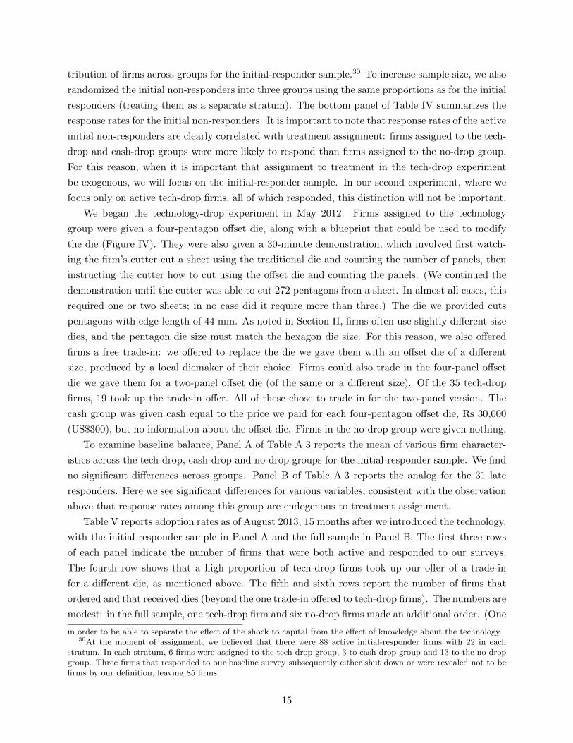
tribution of firms across groups for the initial-responder sample.30 To increase sample size, we also

randomized the initial non-responders into three groups using the same proportions as for the initial

responders (treating them as a separate stratum). The bottom panel of Table IV summarizes the

response rates for the initial non-responders. It is important to note that response rates of the active

initial non-responders are clearly correlated with treatment assignment: firms assigned to the tech-

drop and cash-drop groups were more likely to respond than firms assigned to the no-drop group.

For this reason, when it is important that assignment to treatment in the tech-drop experiment

be exogenous, we will focus on the initial-responder sample. In our second experiment, where we

focus only on active tech-drop firms, all of which responded, this distinction will not be important.

We began the technology-drop experiment in May 2012. Firms assigned to the technology

group were given a four-pentagon offset die, along with a blueprint that could be used to modify

the die (Figure IV). They were also given a 30-minute demonstration, which involved first watch-

ing the firm’s cutter cut a sheet using the traditional die and counting the number of panels, then

instructing the cutter how to cut using the offset die and counting the panels. (We continued the

demonstration until the cutter was able to cut 272 pentagons from a sheet. In almost all cases, this

required one or two sheets; in no case did it require more than three.) The die we provided cuts

pentagons with edge-length of 44 mm. As noted in Section II, firms often use slightly different size

dies, and the pentagon die size must match the hexagon die size. For this reason, we also offered

firms a free trade-in: we offered to replace the die we gave them with an offset die of a different

size, produced by a local diemaker of their choice. Firms could also trade in the four-panel offset

die we gave them for a two-panel offset die (of the same or a different size). Of the 35 tech-drop

firms, 19 took up the trade-in offer. All of these chose to trade in for the two-panel version. The

cash group was given cash equal to the price we paid for each four-pentagon offset die, Rs 30,000

(US$300), but no information about the offset die. Firms in the no-drop group were given nothing.

To examine baseline balance, Panel A of Table A.3 reports the mean of various firm character-

istics across the tech-drop, cash-drop and no-drop groups for the initial-responder sample. We find

no significant differences across groups. Panel B of Table A.3 reports the analog for the 31 late

responders. Here we see significant differences for various variables, consistent with the observation

above that response rates among this group are endogenous to treatment assignment.

Table V reports adoption rates as of August 2013, 15 months after we introduced the technology,

with the initial-responder sample in Panel A and the full sample in Panel B. The first three rows

of each panel indicate the number of firms that were both active and responded to our surveys.

The fourth row shows that a high proportion of tech-drop firms took up our offer of a trade-in

for a different die, as mentioned above. The fifth and sixth rows report the number of firms that

ordered and that received dies (beyond the one trade-in offered to tech-drop firms). The numbers are

modest: in the full sample, one tech-drop firm and six no-drop firms made an additional order. (One

in order to be able to separate the effect of the shock to capital from the effect of knowledge about the technology.30At the moment of assignment, we believed that there were 88 active initial-responder firms with 22 in each

stratum. In each stratum, 6 firms were assigned to the tech-drop group, 3 to cash-drop group and 13 to the no-dropgroup. Three firms that responded to our baseline survey subsequently either shut down or were revealed not to befirms by our definition, leaving 85 firms.

15

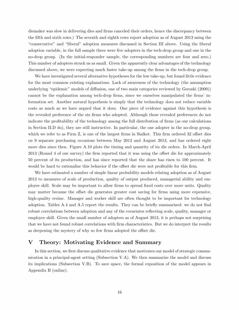
diemaker was slow in delivering dies and firms canceled their orders, hence the discrepancy between

the fifth and sixth rows.) The seventh and eighth rows report adoption as of August 2013 using the

“conservative” and “liberal” adoption measures discussed in Section III above. Using the liberal

adoption variable, in the full sample there were five adopters in the tech-drop group and one in the

no-drop group. (In the initial-responder sample, the corresponding numbers are four and zero.)

This number of adopters struck us as small. Given the apparently clear advantages of the technology

discussed above, we were expecting much faster take-up among the firms in the tech-drop group.

We have investigated several alternative hypotheses for the low take-up, but found little evidence

for the most common existing explanations. Lack of awareness of the technology (the assumption

underlying “epidemic” models of diffusion, one of two main categories reviewed by Geroski (2000))

cannot be the explanation among tech-drop firms, since we ourselves manipulated the firms’ in-

formation set. Another natural hypothesis is simply that the technology does not reduce variable

costs as much as we have argued that it does. One piece of evidence against this hypothesis is

the revealed preference of the six firms who adopted. Although these revealed preferences do not

indicate the profitability of the technology among the full distribution of firms (as our calculations

in Section II.D do), they are still instructive. In particular, the one adopter in the no-drop group,

which we refer to as Firm Z, is one of the largest firms in Sialkot. This firm ordered 32 offset dies

on 9 separate purchasing occasions between May 2012 and August 2013, and has ordered eight

more dies since then. Figure A.10 plots the timing and quantity of its die orders. In March-April

2013 (Round 4 of our survey) the firm reported that it was using the offset die for approximately

50 percent of its production, and has since reported that the share has risen to 100 percent. It

would be hard to rationalize this behavior if the offset die were not profitable for this firm.

We have estimated a number of simple linear probability models relating adoption as of August

2013 to measures of scale of production, quality of output produced, managerial ability and em-

ployee skill. Scale may be important to allow firms to spread fixed costs over more units. Quality

may matter because the offset die generates greater cost saving for firms using more expensive,

high-quality rexine. Manager and worker skill are often thought to be important for technology

adoption. Tables A.4 and A.5 report the results. They can be briefly summarized: we do not find

robust correlations between adoption and any of the covariates reflecting scale, quality, manager or

employee skill. Given the small number of adopters as of August 2013, it is perhaps not surprising

that we have not found robust correlations with firm characteristics. But we do interpret the results

as deepening the mystery of why so few firms adopted the offset die.

V Theory: Motivating Evidence and Summary

In this section, we first discuss qualitative evidence that motivates our model of strategic commu-

nication in a principal-agent setting (Subsection V.A). We then summarize the model and discuss

its implications (Subsection V.B). To save space, the formal exposition of the model appears in

Appendix B (online).

16

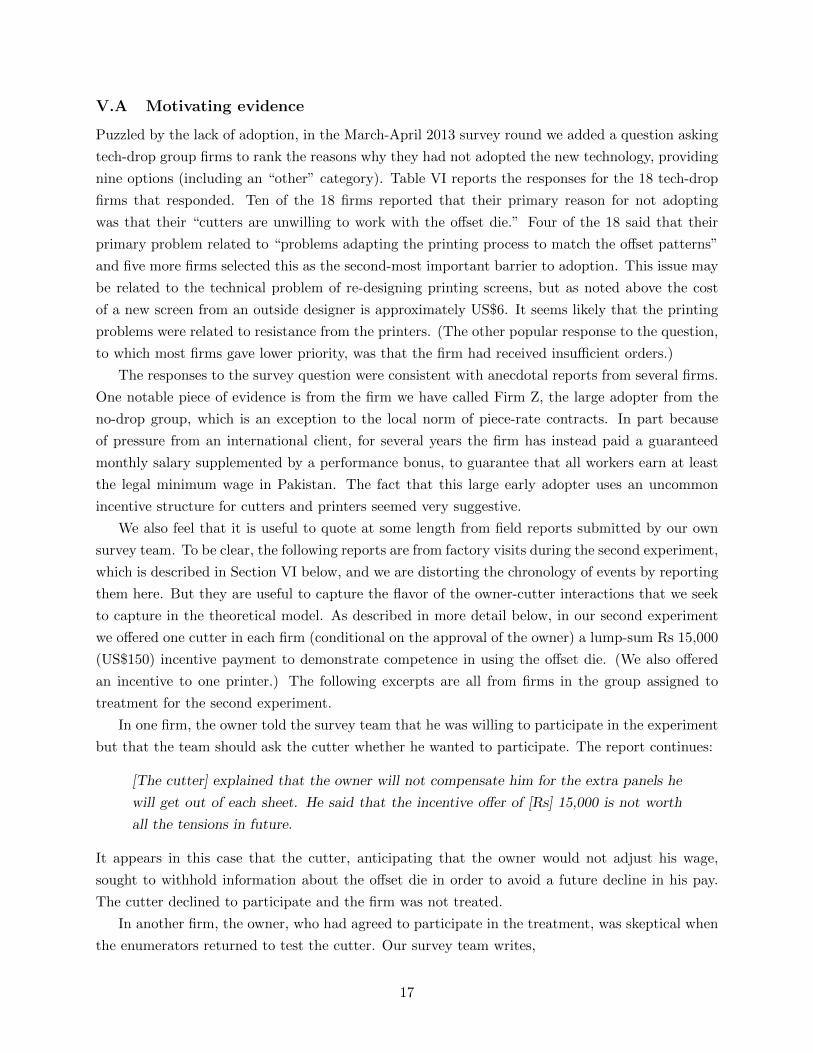
V.A Motivating evidence

Puzzled by the lack of adoption, in the March-April 2013 survey round we added a question asking

tech-drop group firms to rank the reasons why they had not adopted the new technology, providing

nine options (including an “other” category). Table VI reports the responses for the 18 tech-drop

firms that responded. Ten of the 18 firms reported that their primary reason for not adopting

was that their “cutters are unwilling to work with the offset die.” Four of the 18 said that their

primary problem related to “problems adapting the printing process to match the offset patterns”

and five more firms selected this as the second-most important barrier to adoption. This issue may

be related to the technical problem of re-designing printing screens, but as noted above the cost

of a new screen from an outside designer is approximately US$6. It seems likely that the printing

problems were related to resistance from the printers. (The other popular response to the question,

to which most firms gave lower priority, was that the firm had received insufficient orders.)

The responses to the survey question were consistent with anecdotal reports from several firms.

One notable piece of evidence is from the firm we have called Firm Z, the large adopter from the

no-drop group, which is an exception to the local norm of piece-rate contracts. In part because

of pressure from an international client, for several years the firm has instead paid a guaranteed

monthly salary supplemented by a performance bonus, to guarantee that all workers earn at least

the legal minimum wage in Pakistan. The fact that this large early adopter uses an uncommon

incentive structure for cutters and printers seemed very suggestive.

We also feel that it is useful to quote at some length from field reports submitted by our own

survey team. To be clear, the following reports are from factory visits during the second experiment,

which is described in Section VI below, and we are distorting the chronology of events by reporting

them here. But they are useful to capture the flavor of the owner-cutter interactions that we seek

to capture in the theoretical model. As described in more detail below, in our second experiment

we offered one cutter in each firm (conditional on the approval of the owner) a lump-sum Rs 15,000

(US$150) incentive payment to demonstrate competence in using the offset die. (We also offered

an incentive to one printer.) The following excerpts are all from firms in the group assigned to

treatment for the second experiment.

In one firm, the owner told the survey team that he was willing to participate in the experiment

but that the team should ask the cutter whether he wanted to participate. The report continues:

[The cutter] explained that the owner will not compensate him for the extra panels he

will get out of each sheet. He said that the incentive offer of [Rs] 15,000 is not worth

all the tensions in future.

It appears in this case that the cutter, anticipating that the owner would not adjust his wage,

sought to withhold information about the offset die in order to avoid a future decline in his pay.

The cutter declined to participate and the firm was not treated.

In another firm, the owner, who had agreed to participate in the treatment, was skeptical when

the enumerators returned to test the cutter. Our survey team writes,

17

[The owner] told us that the firm is getting only 2 to 4 extra pentagon panels by using

our offset panel... The owner thinks that the cost savings are not large enough to adopt

the offset die... He allowed us to time the cutter.

The team then continued to the cutting room without the owner.

On entering the cutting area, we saw the cutter practicing with our offset die... We

tested the cutter... He got 279 pentagon pieces in 2 minutes 32 seconds... The cutter

privately told us that he can get 10 to 12 pieces extra by using our offset die.

The owner then arrived in the cutting area.

We informed the owner about the cutter’s performance. The owner asked the cutter

how many more pieces he can get by using the offset die. The cutter replied, “only 2

to 4 extra panels.”

It appears that the cutter had been misinforming the owner. But the cutter did not hide the

performance of the die in the cutting process itself, likely either because it was difficult to do so or

because he did not want to jeopardize his incentive payment.

The owner asked the cutter to cut a sheet in front of him. The cutter got 275 pieces

in 2 minutes 25 seconds. The owner looked satisfied by the cutter’s speed... The owner

requested us to experiment with volleyball dies.

This firm subsequently adopted the offset die.

In a third firm, the owner reported that he had modified the wage he pays to his cutter to make

up for the slower speed of the offset die. Our team writes,

[The owner] said that it takes 1 hour for his cutter to cut 25 sheets with the conventional

die. With the offset die it takes his cutter 15 mins more to cut 25 sheets for which he

pays him [Rs] 100 extra for the day which is not a big deal.

This firm has generally not been cooperative in our survey, and we have not been able to verify

that the firm has produced more than 1,000 balls with the offset die, and for this reason is not

classified as an adopter.

V.B Summary of model

The survey results and qualitative evidence highlight the role of misaligned incentives and suggest

that workers are discouraging some firms from adopting. But this raises two important questions.

First, given that owners should be aware that workers have an incentive to discourage adoption

of the offset dies, why are they influenced by what the workers say? Second, why do owners not

simply offer a different labor contract, to give workers an incentive to support the adoption the

cost-saving technology? To address these questions and to motivate our second experiment, we

develop a model embedding a cheap-talk interaction along the lines of Crawford and Sobel (1982)

18

in a standard principal-agent model. We recognize that other models with misaligned incentives

and an ability of cutters to impose direct costs on firms may generate similar predictions. (See in

particular Dow and Perotti (2013) and Sections 4 and 5 of Garicano and Rayo (2016).) But in our

view the model provides a particularly parsimonious account of the main forces at play. (As noted

above, the full exposition is in Appendix B (online).)

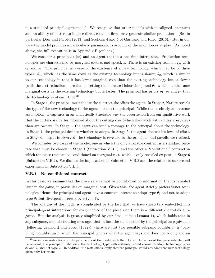
We consider a principal (she) and an agent (he) in a one-time interaction. Production tech-

nologies are characterized by marginal cost, c, and speed, s. There is an existing technology, with

c0 and s0. The principal is aware of the existence of a new technology, which may be of three

types: θ1, which has the same costs as the existing technology but is slower; θ2, which is similar

to our technology in that it has lower marginal cost than the existing technology but is slower

(with the cost reduction more than offsetting the increased labor time); and θ3, which has the same

marginal costs as the existing technology but is faster. The principal has priors ρ1, ρ2 and ρ3 that

the technology is of each type.31

In Stage 1, the principal must choose the contract she offers the agent. In Stage 2, Nature reveals

the type of the new technology to the agent but not the principal. While this is clearly an extreme

assumption, it captures in an analytically tractable way the observation from our qualitative work

that the cutters are better informed about the cutting dies (which they work with all day every day)

than are owners. In Stage 3, the agent can send a message to the principal about the technology.

In Stage 4, the principal decides whether to adopt. In Stage 5, the agent chooses his level of effort.

In Stage 6, output is observed, the technology is revealed to the principal, and payoffs are realized.

We consider two cases of the model, one in which the only available contract is a standard piece

rate that must be chosen in Stage 1 (Subsection V.B.1), and the other a “conditional” contract in

which the piece rate can be conditioned on marginal cost, which is only revealed ex post, in Stage 6

(Subsection V.B.2). We discuss the implications in Subsection V.B.3 and the relation to our second

experiment in Subsection V.B.4.

V.B.1 No conditional contracts

In this case, we assume that the piece rate cannot be conditioned on information that is revealed

later in the game, in particular on marginal cost. Given this, the agent strictly prefers faster tech-

nologies. Hence the principal and agent have a common interest to adopt type θ3 and not to adopt

type θ1 but divergent interests over type θ2.

The analysis of the model is complicated by the fact that we have cheap talk embedded in a

principal-agent interaction: for every choice of the piece rate there is a different cheap-talk sub-

game. But the analysis is greatly simplified by our first lemma (Lemma 1), which holds that in

any subgame, modulo treating messages that induce the same action by the principal as equivalent

(following Crawford and Sobel (1982)), there are just two possible subgame equilibria: a “bab-

bling” equilibrium in which the principal ignores what the agent says and does not adopt; and an

31We impose restrictions on the parameters of the model such that, for all the values of the piece rate that willbe relevant, the principal, if she knew the technology type with certainty, would choose to adopt technology typesθ2 and θ3 and not type θ1. In addition, the restrictions imply that the principal would not adopt the new technologygiven only her priors.

19

“informative” equilibrium in which the agent seeks to encourage adoption of type θ3 and discourage

adoption of types θ1 and θ2, and the principal is influenced by the agent’s message. We place no

restrictions on the richness of the space of possible messages, but as shorthand we will refer to a

message that encourages the principal to adopt as “technology is good” and one that discourages

her as “technology is bad.” In the informative subgame equilibrium (if it exists), if the principal

hears the message “technology is bad”, she infers that the technology is type θ1 or θ2; if “technology

is good”, she infers θ3. One implication of Lemma 1 is that there cannot exist an equilibrium in

which the agent fully reveals the technology type to the principal.

Our key proposition in this case (Proposition 1) holds that there exists an equilibrium in which

the principal offers the same piece rate as under the existing technology, the agent says “technology

is bad” if it is type θ1 or θ2 and “technology is good” if it is type θ3, and the principal follows the

agent’s advice. In particular, if the technology is type θ2 the agent discourages the principal from

adopting and she does not to adopt.32 It is common in the literature on cheap talk to assume that

players will coordinate on the most informative equilibrium in cheap-talk interactions.33 If we adopt

this assumption (for every cheap-talk subgame), then the equilibrium described in Proposition 1 is

unique.

V.B.2 Conditional contracts

In this case, we allow the principal at Stage 0 to pay a fixed cost, G, to be able to offer a contract

that conditions the piece rate on marginal cost, revealed in Stage 6. Given our assumptions, only

type θ2 differs in marginal cost from the existing technology. The conditional contract is useful in

that it enables the principal to offer a higher piece rate if the technology is type θ2. The fixed cost

G can be interpreted as the cost of a commitment device to pay a piece rate above the one that

would be paid for the existing technology (β0), which otherwise the principal would not be able to

credibly commit to. (We discuss other possible interpretations in Section V.B.3 below.)

Our main proposition in this case (Proposition 2) holds that there exists an equilibrium in

which, if the contracting fixed cost G is sufficiently small, the principal pays G and offers a supple-

ment to the piece rate if the technology is revealed to by type θ2. Given the supplement, the agent

wants to adopt the same technologies that the principal wants to adopt, θ2 or θ3, and technologies

of type θ2 are adopted.

“Sufficiently small” for G means less than the expected benefit of adopting technology θ2 rela-

tive to the existing technology, which depends on speed and cost of the technologies as well as the

principal’s prior, ρ2, that the technology is type θ2. If ρ2 is sufficiently low, then the principal will

32A word of explanation about whether the equilibrium involves “misinformation”: formally, the actual wordsthat the agent uses to convey his message are immaterial; what matters is how the principal interprets the message,and in the Proposition-1 equilibrium the principal interprets “technology is bad” to mean “technology is type θ1or θ2.” In this sense, the agent technically does not “misinform” the principal about type θ2 and we avoid usingthis terminology in the theory. But in the empirical setting we have found that workers tend to use particularwords to discourage adoption that paint the type θ2 technology as ineffective, and describing the communication asmisinformation there is more apt.

33Crawford and Sobel (1982) argue that the most informative equilibrium is “a reasonable one for agents tocoordinate on” because it is Pareto-optimal in their setting. Other justifications for the assumption have also beendiscussed in the literature; see e.g. Chen, Kartik, and Sobel (2008).

20

not pay G and the players will be back in the world of the first case, where their interests diverge

and type θ2 will not be adopted. Again, if we assume players coordinate on the most informative

subgame equilibria, then the Proposition-2 equilibrium is unique.

V.B.3 Discussion

Let us come back to the two questions posed at the beginning of the model summary. First, why

are owners influenced by cutters’ messages, given that they should be aware that cutters have an

incentive to resist adoption of our die? The answer from the model is that the interests of the

principal and agent are sufficiently aligned — they have common interests over types θ1 and θ3

— that the agent’s message can be informative. In particular, in the Proposition-1 equilibrium,

the principal can infer whether θ = θ3 or θ ∈ {θ1, θ2}, and this is valuable enough that she pays

attention to the agent’s message, knowing that it may lead her not to adopt type θ2.

Second, why don’t owners offer a labor contract that incentivizes cutters to support the adop-

tion of our die? The model suggests two reasons. One is simply that the principal may be unaware

of the existence of the conditional contract; this corresponds to the no-conditional-contracts case.

The conditional contract may be an organizational innovation that was previously unknown, at

least to some firms, in the same way that our technical innovation was previously unknown.

Another reason, corresponding to the conditional-contracts case, is that the principal is aware

of the conditional contract but perceives the cost of implementing it to be higher than the expected

benefit. The contracting fixed cost, G, can be interpreted in a number of ways. It may be that a

fairness norm has arisen around standard piece-rate contracts, such that any deviation would carry

a morale cost. Or firms may worry that if they offer a higher piece rate in one case, workers will

demand higher rates in others. G can also be interpreted as a cost of a commitment device for the

principal’s pledge to pay the higher piece rate if the technology is type θ2.34 Finally, the fixed cost

can be interpreted in light of the ratchet effect (e.g. Gibbons (1987)). If a worker on a piece-rate

contract discovers a labor-saving innovation, he may not reveal it to the owner if he expects her

to cut the piece rate in response. It may be optimal for the principal to commit to not changing

the piece rate in order to encourage labor-saving innovations. If most innovations in Sialkot are

labor-saving, this may explain why piece rates are sticky and why it may be costly for firms to start

offering conditional contracts — contracts that open the door to ratcheting. In Section VII below,

we discuss the previous cutting innovation in Sialkot, which was labor-saving. It seems plausible

for firms to expect other new technologies to be labor-saving as well, and to be reluctant to modify

piece rates for this reason.

These two possible explanations for the stickiness of labor contracts — that owners are not

aware of the existence of conditional contracts, and that the benefits owners expect do not out-

weigh the costs of adopting them — have similar implications for the players’ behavior. In either

case, the principal offers a pure (non-conditional) piece rate contract and a technology of type θ2 is

34In our model, marginal cost is revealed in Stage 6, after effort has been supplied in Stage 5. Since the game isone-shot, the principal would have an incentive not to pay the higher piece rate as promised. (This incentive would bepresent under the existing technology as well, but it seems plausible that it would be more difficult for firms to avoidpaying the going rate in the industry, which here corresponds to the optimal piece rate under the existing technology.)

21

not adopted. The key point is that, for whatever reason, many owners did not in fact adjust labor

contracts. This left scope for our incentive intervention, described below, to have an effect.

This discussion is related to a broader debate in organizational economics about the underlying

causes of organizational failure, of which the lack of adoption of our dies is arguably an example.

An organization may fail because it was poorly designed ex ante. Or its design may represent an

ex-ante optimal solution to trade-offs between uncertain costs and benefits, but a shock yields a

sub-optimal outcome ex post. In our context, the idea that an owner is simply not aware of the

existence of conditional contracts corresponds to the first view. The idea that the owner perceives

the fixed cost of offering a conditional contract to be greater than the expected benefit of adopting a

type-θ2 technology corresponds to the second. Our preferred interpretation is the latter; we believe

that most owners are aware of the possibility of conditional contracts, but choose not to offer them

because they assign low probability to the arrival of beneficial new technologies like our dies. But

we recognize that the two interpretations predict similar behavior and it is difficult to discriminate

between them empirically.35

V.B.4 Motivation for incentive intervention

Testing the implications of our model presents a number of practical challenges. In principle, one

approach would be to pay the fixed cost, G, for firms and examine whether they change the labor

contract and adopt the technology. But this cost is not observable and depends on complex social

dynamics within firms; it is not clear how much we (the experimenters) would pay, or to whom.

Another approach would be to offer a piece-rate supplement ourselves. But firms are reluctant to

share the detailed production information that would be required to implement such a payment.

The challenges we faced simply in surveying firms indicated to us that it would be impossible to

manipulate the piece rate directly in our second experiment.36

Facing these constraints, we opted for a third approach: we offered a one-time lump-sum pay-

ment to one cutter and one printer per firm, conditional on revealing the offset die to be cost-saving

in front of the owner. (Presumably, other non-monetary inducements such as increased authority

or greater work schedule flexibility could have served a role similar to our one-time lump-sum

payment.) In Appendix B.4, we prove a formal proposition that if such a conditional lump-sum

payment by a third-party experimenter is sufficiently large, then there exists an equilibrium in

which the agent encourages adoption of type θ2 and the principal adopts it, even if she would not

have offered the conditional contract on her own. Intuitively, the incentive payment plays the same

role as the supplement to the piece rate in the conditional-contracts case: it raises the payoff to the

agent of revealing the technology to be type θ2. Empirically, the main implication is that we would

expect a sufficiently large lump-sum incentive payment to increase adoption of the offset die. It is

35A third view should be considered: that the pure (non-conditional) piece rate is a first-best contract (withno misalignment of incentives) ex ante, and the misalignment arises only because of the intervening shock. In ourmodel, this can be interpreted as a limiting case of the second view above, where ex ante the owner is certain thatthe technology is not of type θ2 (that is, ρ2 = 0).

36In the end, one-third of firms chose not to participate in the much less invasive intervention we decided toimplement; see Section VI below for details. This confirmed our earlier belief that firms’ willingness to participatewould be limited.

22

worth noting that “sufficiently large” in this context is relative to the possible wage losses of a single

cutter, not to the revenues or profits of a firm. Indeed, we will see below that a lump-sum incentive

payment that appears small from the point of view of firms has a large effect on adoption.37

VI Experiment 2: The Incentive-Payment Experiment

VI.A Experimental design

Motivated by the theoretical model, we conducted our second experiment, the incentive-payment

experiment, in September-November 2013. To avoid interfering with the process of diffusion to the

non-tech-drop firms that is the focus of our companion project on spillovers (see footnote 28), we

focused on the 35 tech-drop firms (including both initial responders and initial non-responders).

The 31 still-active firms among these were divided into four similarly sized strata:38 (1) firms in the

two smaller strata from the tech-drop experiment that had not yet adopted the die as of August

2013; (2) firms in the two larger strata from the tech-drop experiment that had not yet adopted the

die; (3) firms from the initial non-responder stratum from the tech-drop experiment that had not

yet adopted the die; and (4) firms that had already adopted the die.39 Within each stratum, firms

were randomly assigned with equal proportion to a treatment subgroup (which we call Group A)

and a control subgroup (Group B). There were 15 firms assigned to Group A and 16 to Group B.

To firms in Group B we gave a reminder about the offset die and the new cutting pattern,

and explicitly informed them about the two-pentagon variant of the offset die (which, as noted

above, had proven more popular than the four-pentagon offset die we originally distributed.) We

also offered to do a new demonstration with their cutters. To each firm in Group A, we gave the

same refresher, the same information about the two-pentagon variant, and the same offer of a new

demonstration. In addition, we explained the misalignment of incentives to the owner and offered

to pay one cutter and one printer lump-sum bonuses roughly equivalent to their monthly incomes

— 15,000 Rs (US$150) and 12,000 Rs (US$120), respectively — on the condition that within one

month they demonstrate competence in using the new technology in front of the owner. If the owner

agreed to the intervention, we explained the intervention to one cutter and one printer chosen by

the owner, paid them 1/3 of the incentive payment on the spot, and scheduled a time to return to

test their performance using the die.40

The performance target for cutters was 272 pentagons from a single sheet in three minutes using

37Note, however, that the required size of the lump-sum transfer may vary across workers, depending on individualand firm characteristics. In the first anecdote above, for instance, it appears that the proposed payment was notlarge enough to induce the cutter to report accurately. In all other cases it appears that the proposed transfer waslarge enough to induce cutters to participate in the intervention.

38At the time of randomization, we believed that 34 of these firms were still active. Three of these weresubsequently revealed to have stopped manufacturing soccer balls.

39As shown in Table V, there were four adopters as of August 2013 in the full sample using the conservativedefinition (which is based on our survey data), and five adopters according to the liberal definition (which combinessurvey data with field reports submitted by our enumerators). We stratified using the liberal definition, our preferredmeasure.

40To the extent possible, we attempted to make the payment directly to the cutter and printer. In two cases, theowner insisted that we pay him and that he pass on the money to the employees, and we acceded to this request.

23

the offset die. The target for the printer was 48 pairs of offset pentagons in three minutes.41 We

provided the owner with 20 laminated rexine sheets and printing screens for offset pentagon pairs

for his workers to practice with, and a nominal Rs 5,000 (US$50) to cover additional costs such as

overhead (e.g. electricity while the cutters were practicing). We returned after approximately one

month to test the employees and, upon successful achievement of the performance targets, to pay

the remaining 2/3 of the incentive payments. Without revealing ahead of time that we would do

so, we allowed for a buffer of 30 seconds and 5 pentagons for cutters and 30 seconds for printers.

Table VII evaluates baseline balance by comparing firm characteristics across Group A and

Group B firms at the time of our visit to explain the intervention (September 2013). No differences

in means are statistically significant. It appears that the randomization was successful.42

VI.B Results

Ten of the 15 Group A firms agreed to participate in the experiment.43 Table A.6 reports the times

achieved by the chosen cutter at each firm (all using the two-pentagon variant of the offset die).

The average time was 2 minutes and 52 seconds, approximately 27 percent longer than the typical

time to cut with the traditional die (2 minutes and 15 seconds). For this reason, we believe that the

100 percent increase in labor time factored into the cost calculations in Section II is conservative. In

addition, many cutters expressed confidence that with additional use they could lower their cutting

time. All printers easily achieved their target, consistent with the assumption in Section II that,

despite some printers’ fears, the offset die does not increase labor time for printing.

To measure short-run adoption responses, we carried out a survey round in January-March 2014

(Round 6 of our survey), 2-5 months after the completion of the incentive-payment intervention.

Before turning to the formal regressions, it is useful to examine the raw adoption statistics. Of the

10 Group A firms that agreed to participate in the experiment, two had already adopted the die.

Of the remaining eight firms, five subsequently adopted using the liberal definition (or four using

the conservative definition). Of the 16 Group B firms, three firms had already adopted prior to the

invention. None of the remaining 13 firms adopted in the short run, by either measure. To examine

medium-run responses, we carried out another survey round in October-December 2014 (Round 7

of our survey), 11-13 months after the completion of the intervention. If the technology is beneficial,

as we have argued, one would expect it eventually to be adopted by all firms (once there has been

sufficient social learning, for instance) and there would then be no long-run effect of our incentive

treatment. In this sense, it would be reasonable to expect the medium- and long-run treatment

effect to be smaller than the short-run one. Indeed, by Oct.-Dec. 2014, one initial non-adopter

41The 3-minute targets were chosen after conducting speed tests at two of the pilot firms mentioned in SectionIV. They are approximately 33 percent higher than the time to cut a single sheet using the original die and the timeto print 48 two-pentagon panels cut using the original die.

42Because of an error by our enumerators, one firm that was assigned to Group B was offered the incentive-payment intervention. This occurred while two co-authors of the paper were in the field, and the error was caughtwithin hours of its occurrence. To maintain balance, we randomly selected one as-yet-untreated Group A firmfrom the same stratum and re-assigned it to Group B. As neither firm adopted, our results hold with the originalrandomization (available upon request).

43In two of these 10 firms, it was not possible to complete the printer performance test.

24

in Group B (that is, a Group B firm that had not yet adopted at the start of Experiment 2) had

adopted the die (by either definition).

Table VIII uses the liberal adoption measure to assess formally the impact of the incentive-

payment intervention on adoption rates. All regressions include dummies for the four strata de-

scribed above. Panel A reports impacts on adoption in the short run, and Panel B in the medium

run. Focusing on the short run first, the first-stage estimates (Column 1) indicate, not surpris-

ingly, that assignment to Group A is significantly associated with greater probability of receiving

the incentive-payment treatment; that is, we have a strong first stage. The dependent variable in

Columns 2-4 is a 0/1 indicator for whether a firm has adopted. The OLS estimate of the coefficient

on treatment in Column 2 is positive and significant, but one might be worried about selection

into treatment. The reduced-form (intent-to-treat, ITT) result in Column 3 does not suffer from

such selection issues and indicates a positive and significant (at the 5 percent level) causal relation-

ship between assignment and adoption. The estimate indicates that the probability of adoption

increased by 0.32 among those assigned to treatment (from a baseline of 13 percent).44 The IV

estimate (the effect of treatment on the treated) is substantially higher: 0.48. However, since the

one third of firms who refused the intervention may have chosen to do so because of particularly

large costs of adoption (or small benefits), these IV estimates should be treated with caution. The

medium-run ITT estimate in Panel B is slightly lower at 0.27 (and statistically significant at the

10 percent level) because of the one Group B firm that adopted in the second six-month period

after the intervention. (The number of observations falls in the medium-run results because two

firms exited.) Table IX reports very similar results using the conservative adoption measure — the

short-run ITT is 0.31 and statistically significant at the 5 percent level, and the medium-run ITT

is 0.26 and statistically significant at the 10 percent level.45

To check robustness, Table X reports results using an alternative indicator of adoption: whether

the firm purchased its first offset die (beyond the trade-in that we paid for) after September 1, 2013.

Of the eight firms that accepted the intervention and had not adopted by August 2013, three sub-

sequently purchased their first offset die. (One of these firms had not yet produced with it at the

time of our Oct.-Dec. 2014 survey round.)46 Table X shows that the positive causal effect of the

44An interesting question to consider is how our estimates would differ if we had included the non-tech-drop firmsin our second experiment — that is, if we had offered the technology and incentive payment at the same time to firmsthat had not received the offset die initially. We suspect that the ITT estimate would have been larger among thesefirms. Among the original tech-drop firms, cutters that did not reveal that the technology was a good one beforeExperiment 2 may have been particularly reluctant to do so in Experiment 2, since it would have revealed that theyhad previously been mis-reporting the benefits of the technology. By contrast, if we had given the technology andincentive simultaneously to the original non-tech-drop firms, cutters in those firms would have had no reason to bereluctant. Because of this difference, treating the non-tech-drop firms in Experiment 2 would not have representeda simple increase in sample size; we believe that it would not have been appropriate to pool the data from thetech-drop and non-tech-drop groups.

45Tables A.7-A.9 re-run the results using more stringent adoption thresholds of 5,000, 10,000 or 20,000 balls,respectively (as opposed to the 1,000 ball threshold used in Tables VIII-IX). The results are even stronger becauseno control firm is classified as an adopter using these cutoffs. Note that the adoption rates are the same for the 5000and 10000 cutoffs, so the numbers in those tables are identical to each other.

46In addition, one large Group-A firm that was already classified as an adopter because it was using the offsetcutting pattern for table cutting (see footnote 16), purchased its first die (beyond the four-panel offset die weoriginally gave) following the beginning of our intervention.

25

incentive-payment treatment on adoption is robust to using this alternative measure. As before,

we report both short- and medium-run impacts. The short- and medium-run ITT estimates are

0.27 and 0.28, respectively, and are both statistically significant at the 5 percent level.

It is important to acknowledge that the sample sizes in the incentive-payment experiment are

small. An alternative to large-N statistical inference are permutation tests whose properties are

independent of sample size. (See Bloom et al (2013) for the use of this type of inference in a similar

context.) We determine the proportion of all 25,872,000 possible treatment assignments that would

produce coefficients as large as or larger than the ones we find (holding the observed outcome for

each firm unchanged).47 This procedure does not require asymptotic approximations. Given the

selection discussion above, we focus on the ITT estimates in Column 3 of Tables VIII-X. Figure

A.11 plots the distribution of coefficients obtained from regressing the liberal adoption measure on

assignment to Group A for the millions of possible treatment assignments. Because of the small

number of adopters, there are only a handful of possible coefficients, despite the large number of

possible assignments. For the short run, our estimated ITT is the most extreme coefficient that

could be observed under any treatment assignment and is equal to the critical value for a 1 percent

significance test. For the medium run, where we would expect the treatment effect to have begun

to attenuate, a fraction 0.061 of assignments are more extreme and our point estimate is equal to

the critical value for a 10 percent significance test. Figure A.12 reports the corresponding plots

using the conservative adoption measure. Our short-run ITT estimate lies between the 1 and 5

percent critical values, with a fraction 0.018 of assignments being more extreme. Our medium-run

ITT estimate lies just below the 10 percent critical value with a fraction 0.118 of assignments being

more extreme. Figure A.13 presents a similar analysis for our alternative indicator of adoption, die

purchases. The short-run ITT estimate is the most extreme outcome possible and is equal to the 1

percent critical value. The medium-run ITT estimate is equal to the 5 percent critical value, with

a fraction 0.036 of assignments being more extreme.

To sum up: although the level of significance dips slightly below 90 percent in one of the speci-

fications (using the more conservative adoption measure and the small-sample-robust permutation

test in the medium-run specification, when we would expect the effect to have begun to attenu-

ate), overall the results strongly suggest that, consistent with our theoretical model of misaligned

incentives, the incentive-payment treatment spurred adoption among firms.

VII Additional Evidence on Mechanisms

In this section, we present additional (non-experimental) evidence on two key features of our

theoretical model: wage stickiness and information flows within the firm. So as not to reveal the

existence of the offset die to non-tech-drop firms, most of the questions we discuss were asked only

of the 31 tech-drop firms involved in the second experiment, and we focus on these tech-drop firms

47Within each of the four strata, we assigned treatment status with equal proportion. The stratum of smaller firmscontained 6 firms, the stratum of larger firms contained 12 firms, the stratum of initial non-responders contained 8

firms and the stratum of already-adopters contained 5 firms. This means there are 25, 872, 000 =(63

)(126

)(84

)((52

)+(53

))possible treatment assignments.

26

throughout this section. (This section focuses on responses from Round 7 of our survey, conducted

in Oct.-Dec. 2014.)

To shed light on wage stickiness, we recorded the wages of cutters and printers for each month

between August 2013 and September 2014. Generally, it appears that firms change wages relatively

seldom. Of the 24 tech-drop firms that provided complete information, 10 did not change the head

cutter’s wage at all over the entire 13 month period, a period of 8.4 percent annual inflation

(Table A.10). Thirteen out of 24 did not change the wage for the head printer. This evidence is

corroborated by the survey responses from the head cutters and printers themselves: only 2 out of

15 cutters who responded indicated that their wage had changed during this period, and only 4 out

of 17 printers reported a change. We asked firms why they changed wages, and the responses for the

few firms that provided answers are in Table A.11. The two main reasons cited by owners were (a)

inflation and (b) the change was a regular “end of year” change. Only one firm reported changing

wages because of the offset die. In addition to the reasons discussed in Section V.B.3 above, another

possible reason for the wage stickiness is that it is conventional to use round numbers for piece rates.

Figure A.14 shows that 78 percent of piece rates are 1, 1.5, 2, 2.5, 3 or 4 Rupees per ball. Given

this convention, it may be that wage increases must be reasonably large when they occur. These

several pieces of evidence reinforce the idea that piece rates are sticky, consistent with the ideas (a)

that they are chosen in Stage 1 of the game, prior to the technology arriving, and (b) that there is

a significant cost to adopting contracts that involve changing piece rates.

We also asked owners and head cutters directly why payments were not conditioned on the tech-

nology and whether such a possibility was ever discussed. The reason cited most often by owners

(6 out of 18) is that offering such incentives would lead workers to expect additional incentives in

the future. The next two most common answers were that workers would perceive these incentives

as unfair or that the owners did not think of it (Table A.12). Cutters overwhelmingly state that

they feel it is not their place to make suggestions to the owner about the payment schemes (Table

A.13). In almost no case did the owner report discussing payments to adopt the die with any

employee (Table A.14). Similarly, cutters never report talking to the owner or other co-workers

about payments to adopt the die. These responses are consistent with both of the hypotheses for

lack of adjustment of contracts discussed above: that owners and cutters were largely unaware of

the possibility of conditional contracts, or that both were aware of the contracts but that there

were transaction costs associated with adopting them.

Turning to information flows within the firm, we asked owners if they had ever had a con-

versation with their head cutter, other cutters or head printer about whether to adopt the offset

die.48 It appears that this question did not capture all forms of communication between owners and

cutters. For instance, of the 10 firms that reported “cutters unwilling” as the main reason for not

adopting the technology in Round 4 of our survey (Table VI), only six reported that they had had

48The exact wording of the questions were “Did you have a conversation with [the following employee] aboutwhether you should adopt the offset die?” and “If yes, what did they say?” with response codes “(a) the technologyis beneficial and should be adopted, (b) the technology is not beneficial and should not be adopted, (c) not surewhether the technology is beneficial or not, (d) other ( ).”

27

a conversation with the head cutter about whether to adopt the die. Presumably the remaining

respondents received signals from cutters through less direct means, or were too proud to admit

to taking advice from subordinates. With this caveat, the responses do suggest that owners are

being swayed by the opinions of cutters in their adoption decisions. Ten of 22 respondents reported

consulting with their head cutter about the decision (Table A.15). There is a clear association

between what the cutter recommends and what owners eventually do. Table A.16 reports the rec-

ommendations given by the cutters in the 10 cases where owners report consulting them, and the

firms’ corresponding adoption decisions using the liberal definition. In all three instances where the

head cutter recommended adopting, the firm adopted; in four of the six instances where the head

cutter’s recommendation was negative, the firm did not adopt.49 These responses are consistent

with the assumption in the model that owners are less informed than cutters, and the result that

in some circumstances the principal finds it worthwhile to follow the cutter’s advice.

As mentioned above, additional corroborative evidence for our story comes from firms’ experi-

ence with a previous innovation in the cutting process. Prior to 1994, all firms used a single-panel

die to cut pentagons. In 1994, the first firms began using the two-panel non-offset pentagon die

pictured on the right-hand side of Figure I, referred to in Sialkot as the “back-to-back” die. This

die is much faster than a single-pentagon die, since each strike by the hydraulic press cuts two pen-

tagons, and the die does not appear to have reduced the number of pentagons per sheet. Owners

report that the back-to-back die was adopted much more quickly than our offset die has been, and

with little resistance from cutters. All 14 owners who could recall the speed of adoption indicated

that they adopted the die within six months of hearing about it (Table A.17). Furthermore, 23 out

of the 24 respondents report there was no resistance among cutters to adopt this die (Table A.18)

and very few firms changed their payment structure in any way (Table A.19). Relating this evi-

dence to our theory, the back-to-back die can be interpreted as corresponding to technology type θ3

(equal marginal cost but faster than the existing technology), which both principal and agent want

to adopt. The fact that the back-to-back die was adopted quickly and with little resistance from

cutters reinforces two ideas from the theory: first, that cutters’ and owners’ interests over some new

technologies coincide (a precondition for informative communication); and second, that the mis-

alignment of incentives for our offset die is (at least in part) responsible for the slow adoption of it.

VIII Alternative Hypotheses

In this section, we examine what we consider to be the two leading competing explanations for

the results of our second experiment: (1) that we mechanically induced firms to adopt by subsidiz-

ing the fixed costs of adoption, rather than by aligning incentives and inducing information flows

within firms; and (2) that we simply increased the salience of the new technology and this in itself

led firms to adopt.

49Using the conservative definition, in five of the six cases the firm did not adopt.

28

VIII.A Subsidies for fixed costs

Suppose in our model that the principal and agent had the same information about the technology.

The owner would then simply weigh the expected variable cost reduction from the new technol-

ogy against the fixed costs of adoption, F . These fixed costs might include a lump-sum bonus

to workers to compensate them for a learning period in which their incomes are reduced. Our

incentive-payment experiment could be seen as providing a subsidy for these fixed costs, and the

subsidy may itself have induced the owner to adopt.

Is this a quantitatively plausible explanation of our findings? To organize our thinking about

this question, we can write the present discounted value of expected additional profit from adoption

for firm f as follows:

Πf = −Ff + P

∞∑t=1

NV Bf

(1 + r)t= −Ff + P

(NV Bf

r

)(1)

where Πf is expected profit, Ff are fixed costs of adoption, which must be paid up front and may

be firm-specific; P is the probability perceived by the firm that the technology works as we said it

does; NV Bf are net variable benefits per cutter per month; and r is the market interest rate.50 Net

Variable Benefits can be calculated for each firm following the method of Section II.D; we assume

that these are constant over time. For firms that did not have to buy the die (i.e. the tech-drop

firms) a conservative estimate of “observed” fixed costs is Rs 10,800/US$108 to cover the cost of

making new screens and purchasing a new combing die. (See Section II.D.) In this section, we make

the assumption that the Rs 32,000/US$320 we paid in the incentive-payment treatment were also

necessary and part of the true fixed cost of adoption.51 We thus take the total observed fixed costs

to be Rs 42,800/US$428.52 Including the incentive payments in fixed costs seems conservative; in

the incentive-payment experiment, only one worker felt that the payment was insufficient to cover

his costs of adoption, suggesting that the incentive payments were greater than the “training” cost

faced by workers in the great majority of firms.

As a first step toward answering the quantitative plausibility question, suppose that there is no

uncertainty about the technology (i.e. P = 1) and no unobserved fixed costs (i.e. no fixed costs

beyond the US$428 mentioned above.) Under these assumptions, equation (1) can be reconciled

with non-adoption only if firms face extremely high interest rates and hence have a small effec-

50Here we are abstracting from the possibility that firms can learn from others about the profitability of adoption,which would tend to lead them to delay adoption (and wait for others to adopt), as emphasized by Foster andRosenzweig (1995). Such an effect could help to explain low initial adoption, but not the large increase in adoptionin response to our second experiment, and the argument of this section that our subsidies were too small to generatethe latter would continue to hold in a more complex social-learning model.

51As discussed in Section VI.A, we paid Rs 15,000/US$150 to the cutter, Rs 12,000/US$120 to the printer, plusRs 5,000/US$50 to the owner to cover overhead. In Section II.D, we assumed that workers wages went up by 100percent to compensate them for using the slower technology. The discussions in Sections V and VII suggest thatmany firms do not adjust their wages and so in this section we assume that firms make no changes in piece ratesbut make a one-off lump-sum payment to cutters and printers of the same size as in our Experiment 2.

52We take these to be the fixed costs per cutter. This is a conservative assumption since it is possible that firmscould, for example, share the combing machine across cutters.

29

tive discount factor 1/(1 + r).53 The values of firm-specific interest rates that set Πf = 0 in (1)

represent lower bounds on the firm-specific interest rates for non-adopters. At the 10th percentile,

the lower bound is 13.8 percent per month; at the 90th percentile, the lower bound is 134 percent

per month. We asked firms explicitly about the interest rates they face, and the responses ranged

from 9 percent to 25 percent per year ; these are an order of magnitude lower than the implied

lower bound for most firms. That is, in the absence of both uncertainty about the technology and

unobserved fixed costs, the interest rates (or rate of discounting) that would be required to explain

the low initial rates of adoption appear to be implausibly high.

This argument leaves open the possibility that some combination of uncertainty and unobserved

fixed costs can account for the low initial rates of adoption we observed. To address this possibility,

we take a different approach: we allow for both uncertainty and unobserved fixed costs and ask

whether these can explain both the low rates of initial adoption and the magnitude of the response

to our incentive-payment intervention. The unobserved fixed costs may represent attention costs

for the owner or psychic costs involved in changing established routines. We assume, conservatively,

that the interest rate is the highest of the self-reported interest rates, 25 percent per year. As a

benchmark, we assume that owners place a 50 percent probability on the event that the technology

works as we described (i.e. P = 0.5); we consider alternative priors below. Under these assump-

tions, we can place bounds on the values of unobserved fixed costs that can explain the behavior

we observe. In particular, from (1), if a firm does not adopt initially, it must be that Πf < 0 and

hence that Ff > (0.5)NV Bf

0.0187 . (A 25 percent annualized interest rate corresponds to a 1.87 percent

monthly rate.) If a firm adopts in response to the incentive-payment experiment, it must be that

Πf > 0 after the US$320 reduction in fixed costs, and hence that Ff < (0.5)NV Bf

0.0187 + 320. These

bounds on fixed costs are plotted by rank in Figure V for the 31 firms in the incentive-payment

experiment (using the liberal adoption measure). The solid black bars indicate upper bounds on

fixed costs for the initial adopters (for which we can only calculate upper bounds). The white

bars indicate lower bounds for the never-adopters (for which we can only calculate lower bounds).

The solid grey bars indicate lower bounds for initial non-adopters that adopted in response to the

incentive treatment (i.e compliers in Experiment 2); the black outlines above the solid grey bars

indicate upper bounds for these firms. The figure highlights that the US$320 subsidy (indicated

by the distance between the top of the solid grey bars and the black outlines just above them) is

small relative to the implied lower bound on fixed costs for almost all initial non-adopters.

In this context, the key question is whether a plausible distribution of unobserved fixed costs

is consistent with the adoption responses and implied bounds illustrated in the figure. It turns out

that if we impose even minimal structure on the distribution of unobserved fixed costs then it is very

unlikely that the distribution would generate both the initial lack of adoption (which requires that

unobserved fixed costs be large) and the large response to the second experiment (which requires

that US$320 make a significant difference to the adoption decisions of a large number of firms).

53This is another way of stating the argument from Section II.D that the observable fixed costs of adoption canbe recouped within a relatively short amount of time by almost all firms.

30

Suppose that fixed costs are distributed log normally:

ln(Ff ) = µ+ εf (2)

where εf ∼ N (0, σ2ε). Using maximum likelihood, we can estimate the values of µ and the error

variance, σ2ε , that can best account for the observed adoption responses in both experiments.54

Panel A of Table XI reports these estimates µ̂ and σ̂2ε under six priors ranging from P = 0.01 to

P = 1. With these estimates in hand, we can ask: what is the ITT estimate we would obtain from

a US$320 subsidy on adoption, the size of the payment in Experiment 2? To answer this question

we use µ̂ and σ̂2ε to simulate fixed cost draws 1,000 times, with Figure A.15 displaying the full

distribution of Group A firms switching from non-adoption to adoption as a result of a US$320

payment. In Panel B of Table XI, we report the average ITT estimate and the standard deviation

from these simulations. The ITT estimates range between 0.01 and 0.10 for priors between P = 1

and P = 0.05, much lower than the 0.32 we obtained in our incentive-payment experiment (see

Panel A of Table VIII, Column 3).55 Even for the most pessimistic prior of P = 0.01, we only

obtain an ITT of 0.24. Although such a low prior is theoretically possible, it seems unrealistically

pessimistic given the nature of the technology.56 In summary, it appears that if unobserved fixed

costs are the reason for low adoption in Experiment 1, a US$320 subsidy alone cannot plausibly

explain the magnitude of the increase in adoption we observed in Experiment 2.

54We use the short-run liberal adoption rates for this exercise. Let adopt1f denote an indicator if firm f hadadopted the technology in Experiment 1, and adopt2f an analogous indicator for adoption after Experiment 2. Thelog likelihood function for Group A firms is:

L(µ, σε) =∑f

(1− adopt1f )(adopt2f ) ln

Φ

ln[P(

NV Bf

0.0187

)+ 320

]− µ

σε

− Φ

ln[P(

NV Bf

0.0187

)]− µ

σε

+(1− adopt1f )(1− adopt2f ) ln

1− Φ

ln[P(

NV Bf

0.0187

)+ 320

]− µ

σε

(3)

+(adopt1f ) ln

Φ

ln[P(

NV Bf

0.0187

)]− µ

σε

The first expression on the right-hand-side of (3) captures the contribution to the likelihood of initial non-adopterGroup-A firms who are induced to switch from non-adoption to adoption because of the $320 subsidy. The secondexpression captures initial non-adopter Group-A firms who are not induced to switch adoption status. The thirdexpression is the contribution of initial adopter firms. For Group-B firms, the likelihood function is the same exceptadopt2f = 0 ∀f and there is no US$320 payment inside the argument of the normal CDF, Φ(.). We pool both groupswhen maximizing the likelihood function.

55Panel C of Table XI reports the corresponding probabilities that five or more Group A firms adopt in theshort-run (recall that the incentive-payment treatment induced five adopters according to the liberal adoptionmeasure). The probability of observing an increase in adoption of that magnitude is exceedingly low, between 0.000and 0.013, for all but the most pessimistic prior of P = 0.01.

56Recall that we visited each treatment firm and performed a demonstration of the technology in front of theowner. This demonstration involved having the firm’s cutter cut using the traditional die and count the pentagonsand then cut using the offset die and count the pentagons. The latter was repeated until the cutter achieved272 pentagons from a sheet. In no case did this require more than three sheets. The nature of the technology issufficiently transparent that, even if the owners were not convinced of all aspects of the technology, it seems to usimplausible that they placed less than 1 percent probability on the fact that the technology worked as we said it did.

31

VIII.B Salience

A second alternative explanation is that the incentive-payment treatment increased the salience of

the new technology and that this itself led firms to adopt, independent of any effects on information

flows within the firm. There are two variants of this explanation. One variant is that the reminder

about the technology during the incentive-intervention visit itself “nudged” firms into adoption.

This variant seems an unlikely explanation. We gave the same reminder to the control firms for

the incentive intervention (Group B firms) and we saw no firms adopt in the next six months as

a result. Also, it is worth noting that we visited all of the tech-drop firms multiple times in our

survey rounds. During each of these visits, we discussed the new technology with them and if they

were not using it we asked why.

A subtler variant of the salience story is that by putting more money on the table we sent a

stronger signal about our own beliefs about the efficacy of our technology, and that this in turn

led firms to update their priors about the technology, inducing some firms to adopt. While this

explanation is sufficiently flexible that it is difficult to dismiss definitively, it also seems unlikely

to have played a major role. We believe that it was clear to firms from the outset, in the initial

technology-drop implementation, that we thought that the technology was effective. We then re-

turned to each firm numerous times and in the case of the tech-drop firms discussed the offset die

each time. The amount of money we spent on surveying each firm far exceeded the US$320 pay-

ment in the incentive intervention. In short, while in retrospect it seems clear that many owners

did not believe us when we told them that the technology works, it does not appear that their

skepticism was based on their beliefs about how strongly we held our beliefs, or that the US$320

affected their beliefs about how strongly we held our beliefs. It seems more likely that they simply

thought all along that we had insufficient knowledge and experience in the industry, and hence that

our (strongly held) confidence in the technology was misplaced.

IX Conclusion

This paper has two basic empirical findings. First, despite the evident advantages of the technol-

ogy we invented, a surprisingly small number of firms have adopted it, even among the set of firms

that we gave it to. This is consistent with a long tradition of research that has found diffusion to be

slow for many technologies, but given the characteristics of our technology — low fixed costs, mini-

mal required changes to other aspects of the production process, easily measured cost advantages —

the low adoption rate seems particularly puzzling. Second, with a modest change to the incentives of

key employees in the firm — very small in monetary terms relative to firms’ revenues and the bene-

fits of adoption — we induced a statistically significant increase in adoption. This is consistent with

the hypothesis that a misalignment of incentives within the firm is an important barrier to adoption.

Although we do not observe all of the communication between employees and owners, it appears that

at least one way that employees have resisted the adoption of our new technology is by misinforming

owners about the value of the technology. It further appears that the incentive-payment interven-

tion had a significant effect because it induced workers to reveal the benefits of the technology.

32

A natural question is why many owners did not simply change the payment scheme on their own,

to give employees a greater incentive to adopt the new technology. Survey evidence indicates that

some firms are not aware of the availability of alternative payment schemes, and that many firms

believe that there are non-trivial transaction costs involved in changing contracts, even implicit ones.

One would expect owners to weigh any costs of modifying contracts against the expected benefits

of adopting new technologies. If owners have low priors that a new technology is beneficial (or that

a beneficial new technology will arrive in the future), they may rationally be unwilling to pay even

quite small transaction costs. Although it is difficult for us to distinguish empirically between lack

of awareness of alternative contracts and stickiness of contracts as explanations for why owners did

not change payment schemes, the key point is that many owners did not in fact change schemes

and this left scope for our very modest incentive intervention to have a large effect on adoption.

Our study carried out a particular intervention with a particular technology in a particular

sector. This naturally raises questions about external validity. For example, both of our experi-

ments were relatively “hands-off”: we gave limited advice to firms after the initial demonstration

in the first experiment, or the incentive payment in the second. Would organizational barriers

still hinder adoption if the innovators (or their salespeople) had financial incentives to work with

firms to promote adoption? We strongly suspect so, since there would still be costs associated with

overcoming such barriers, and it is not clear that innovators’ incentives would be strong enough

to induce them to pay such costs for firms, or that the firms themselves would be willing ex ante

to grant innovators the access and time to identify the barriers and resolve them (especially if

they receive negative feedback about the technology from their own workers).57 Nevertheless, we

recognize that more research is required, in other sectors, with other technologies, to determine to

what extent our findings in Sialkot can be generalized.

With that caveat, we believe that three implications of our study are likely to apply more

broadly. First, we have provided reasonably direct evidence of a complementarity, in the sense

of Milgrom and Roberts (1990, 1995), between a technological innovation (the offset die) and an

organizational innovation (conditional wage contracts). We suspect that similar complementari-

ties between technical and organizational innovations exist in many other settings, and that it is

common for technology adoption to require organizational changes in order to be successful.

Second, there appears to be a form of inertia in employment relationships that can hinder

technological change. We have argued that firms’ choices of labor contracts depend on the rate

at which beneficial new technologies are expected to arrive. It also appears that labor contracts,

once established, are difficult to modify. The implication is that firms and industries that evolve

in technologically stable environments may be less able to adapt to technological change than new

firms and industries, or firms and industries that evolve in technologically dynamic environments.

Simple piece-rate contracts may well have been optimal for firms in Sialkot before we showed up,

but the very fact that firms in Sialkot have been producing for decades using them may itself have

57We also believe that our results are directly relevant to a number of real-world settings in which innovationsare developed by non-profits and public-sector entities (e.g. agricultural extension services) that have weak financialincentives but that nonetheless aim to promote adoption of beneficial new technologies.

33

contributed to low adoption rates of the offset die.

Finally, it seems likely that for technology adoption to be successful employees need to have an

expectation that they will share in the gains from adoption. Such an expectation may be generated

by a variety of different types of contracts, implicit or explicit. But to the extent that firms must rely

on the knowledge of shopfloor workers about the value of new technologies or how best to implement

them, it appears to be important that some sort of credible gain-sharing mechanism be in place.

References

Aghion, P., and J. Tirole (1997): “Formal and Real Authority in Organizations,” Journal of PoliticalEconomy, 105(1), 1–29.

Anderson, S. T., and R. G. Newell (2004): “Information Programs for Technology Adoption: TheCase of Energy-Efficiency Audits,” Resource and Energy Economics, 26(1), 27 – 50.

Andridge, R. R., and R. A. Little (2010): “A Review of Hot Deck Imputation for Survey Non-response,”International Statistics Review, 78(1), 40–64.

Atkin, D., A. Chaudhry, S. Chaudry, A. K. Khandelwal, T. Raza, and E. Verhoogen (2016):“On the Origins and Development of Pakistan’s Soccer-Ball Cluster,” World Bank Economic Review(ABCDE Conference Papers & Proceedings).

Atkin, D., A. Chaudhry, S. Chaudry, A. K. Khandelwal, and E. Verhoogen (2015): “Mark-upand Cost Dispersion across Firms: Direct Evidence from Producer Surveys in Pakistan,” AmericanEconomic Review Papers & Proceedings, 105(5), 537–544.

Bandiera, O., I. Barankay, and I. Rasul (2005): “Social Preferences and the Response to Incentives:Evidence from Personnel Data,” Quarterly Journal of Economics, 120(3), 917–962.

(2007): “Incentives for Managers and Inequality among Workers: Evidence from a Firm-LevelExperiment,” Quarterly Journal of Economics, 122(2), 729–773.

(2009): “Social Connections and Incentives in the Workplace: Evidence from Personnel Data,”Econometrica, 77(4), 1047–1094.

Bandiera, O., and I. Rasul (2006): “Social Networks and Technology Adoption in NorthernMozambique,” Economic Journal, 116(514), 869 – 902.

Beaman, L., A. Ben-Yishay, J. Magruder, and A. M. Mobarak (2015): “Can Network Theory-basedTargeting Increase Technology Adoption?,” Unpub. paper, Northwestern Univ.

Beaman, L., J. Magruder, and J. Robinson (2014): “Minding Small Change among Small Firms inKenya,” Journal of Development Economics, 108, 69 – 86.

BenYishay, A., and A. M. Mobarak (2014): “Social Learning and Communication,” NBER workingpaper no. 20139.

Bloom, N., B. Eifert, A. Mahajan, D. McKenzie, and J. Roberts (2013): “Does ManagementMatter? Evidence from India,” Quarterly Journal of Economics, 128(1), 1–51.

Bloom, N., and J. Van Reenen (2007): “Measuring and Explaining Management Practices Across Firmsand Countries,” Quarterly Journal of Economics, 122(4), 1351–1408.

(2010): “Why Do Management Practices Differ across Firms and Countries?,” Journal of EconomicPerspectives, 24(1), 203–24.

Bresnahan, T. F., and M. Trajtenberg (1995): “General Purpose Technologies: ‘Engines ofGrowth’?,” Journal of Econometrics, 65(1), 83 – 108.

Carmichael, H. L., and W. B. MacLeod (2000): “Worker Cooperation and the Ratchet Effect,”Journal of Labor Economics, 18(1), 1–19.

Chen, Y., N. Kartik, and J. Sobel (2008): “Selecting Cheap-Talk Equilibria,” Econometrica, 76(1),117–136.

Clawson, D. (1980): Bureaucracy and the Labor Process: The Transformation of US Industry, 1860-1920.Monthly Review Press New York.

34

Cohen, J., and P. Dupas (2010): “Free Distribution or Cost-Sharing? Evidence from a RandomizedMalaria Prevention Experiment,” Quarterly Journal of Economics, 125(1), 1–45.

Coleman, James, E. K., and H. Menzel (1966): Medical Innovation: A Diffusion Study. Bobbs-Merrill,New York.

Conley, T., and C. Udry (2010): “Learning about a New Technology: Pineapple in Ghana,” AmericanEconomic Review, 100(1), 35–69.

Crawford, V. P., and J. Sobel (1982): “Strategic Information Transmission,” Econometrica, 50(6),1431–1451.

David, P. A. (1990): “The Dynamo and the Computer: An Historical Perspective on the ModernProductivity Paradox,” American Economic Review Papers and Proceedings, 80(2), 355–61.

de Mel, S., D. J. McKenzie, and C. Woodruff (2008): “Returns to Capital in Microenterprises:Evidence from a Field Experiment,” Quarterly Journal of Economics, 123(4), 1329–1372.

Dearden, J., B. W. Ickes, and L. Samuelson (1990): “To Innovate or Not to Innovate: Incentives andInnovation in Hierarchies,” American Economic Review, 80(5), 1105–1124.

Dessein, W. (2002): “Authority and Communication in Organizations,” Review of Economic Studies,69(4), 811 – 838.

Dow, J., and E. Perotti (2013): “Resistance to Change,” Unpub. paper, London Business School.

Duflo, E., M. Kremer, and J. Robinson (2011): “Nudging Farmers to Use Fertilizer: Theory andExperimental Evidence from Kenya,” American Economic Review, 101(6), 2350–2390.

Dupas, P. (2014): “Short-run Subsidies and Long-Run Adoption of New Health Products: Evidence froma Field Experiment,” Econometrica, 82(1), 197–228.

Edwards, R. C. (1979): Contested Terrain: The Transformation of the Workplace in the TwentiethCentury. Basic Books.

Emerick, K., A. de Janvry, E. Sadoulet, and M. H. Dar (2016): “Technological Innovations,Downside Risk, and the Modernization of Agriculture,” American Economic Review, 106(6), 1537–61.

Foster, A. D., and M. R. Rosenzweig (1995): “Learning by Doing and Learning from Others: HumanCapital and Technical Change in Agriculture,” Journal of Political Economy, 103(6), 1176–1209.

Fowlie, M., M. Greenstone, and C. Wolfram (2015a): “Are the Non-monetary Costs of EnergyEfficiency Investments Large? Understanding Low Take-Up of a Free Energy Efficiency Program,”American Economic Review, 105(5), 201–04.

(2015b): “Do Energy Efficiency Investments Deliver? Evidence from the Weatherization AssistanceProgram,” Unpub. paper, UC Berkeley.

Freeman, R. B., and M. M. Kleiner (2005): “The Last American Shoe Manufacturers: DecreasingProductivity and Increasing Profits in the Shift from Piece Rates to Continuous Flow Production,”Industrial Relations: A Journal of Economy and Society, 44(2), 307–330.

Garicano, L., and L. Rayo (2016): “Why Organizations Fail: Models and Cases,” Journal of EconomicLiterature, 54(1), 137–192.

Geroski, P. A. (2000): “Models of Technology Diffusion,” Research Policy, 29(4–5), 603 – 625.

Gibbons, R. (1987): “Piece-Rate Incentive Schemes,” Journal of Labor Economics, pp. 413–429.

Gibbons, R., and J. Roberts (2013): “Economic Theories of Incentives in Organizations,” in Handbookof Organizational Economics, ed. by R. Gibbons, and J. Roberts. Princeton: Princeton University Press.

Griliches, Z. (1957): “Hybrid Corn: An Exploration in the Economics of Technological Change,”Econometrica, 25(4), 501–22.

Hall, B. (2005): “Innovation and Diffusion,” in Oxford Handbook of Innovation, ed. by J. Fagerberg, D. C.Mowery, and R. R. Nelson, pp. 459–484. Oxford University Press.

Hall, B., and B. Khan (2003): “Adoption of New Technology,” in New Economy Handbook, ed. by D. C.Jones. Academic Press, San Diego.

Hanna, R., S. Mullainathan, and J. Schwartzstein (2014): “Learning Through Noticing: Theoryand Experimental Evidence in Farming,” Quarterly Journal of Economics, 129(3), 1311–1353.

Hardy, M., and J. McCasland (2016): “It Takes Two: Experimental Evidence on the Determinants ofTechnology Diffusion,” Unpub. paper, University of British Columbia.

Holmstrom, B., and P. Milgrom (1991): “Multi-Task Principal-Agent Analyses: Incentive Contracts,

35

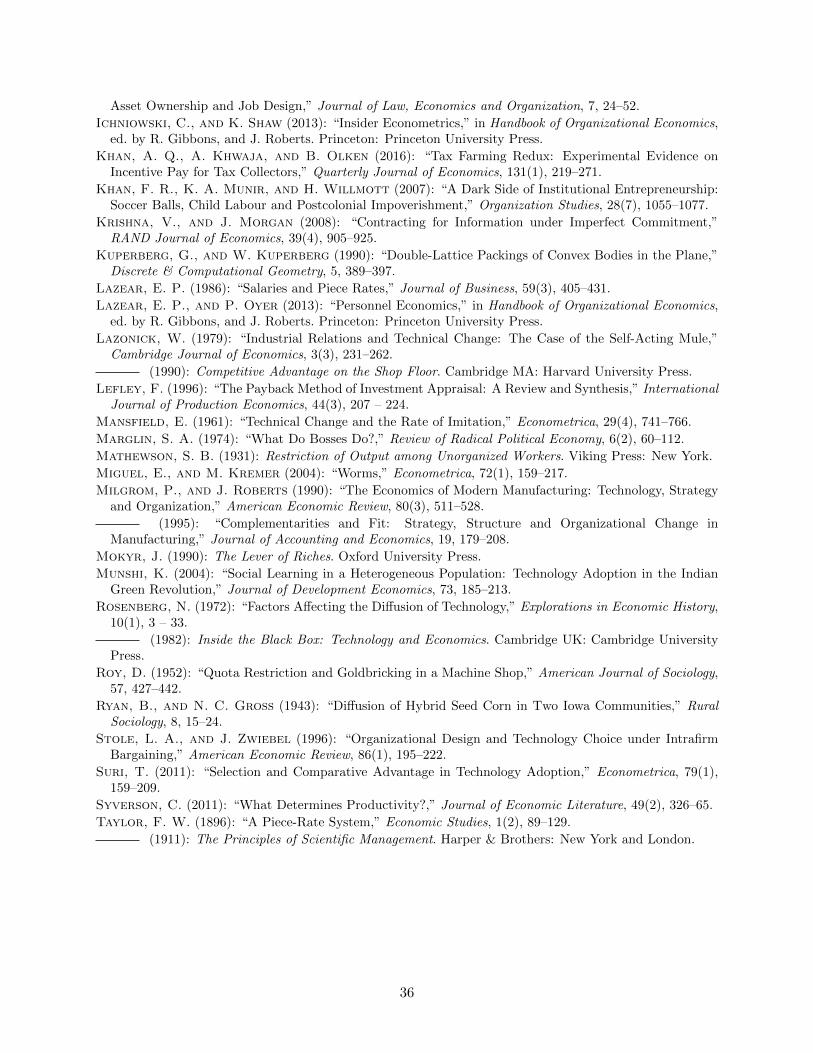
Asset Ownership and Job Design,” Journal of Law, Economics and Organization, 7, 24–52.

Ichniowski, C., and K. Shaw (2013): “Insider Econometrics,” in Handbook of Organizational Economics,ed. by R. Gibbons, and J. Roberts. Princeton: Princeton University Press.

Khan, A. Q., A. Khwaja, and B. Olken (2016): “Tax Farming Redux: Experimental Evidence onIncentive Pay for Tax Collectors,” Quarterly Journal of Economics, 131(1), 219–271.

Khan, F. R., K. A. Munir, and H. Willmott (2007): “A Dark Side of Institutional Entrepreneurship:Soccer Balls, Child Labour and Postcolonial Impoverishment,” Organization Studies, 28(7), 1055–1077.

Krishna, V., and J. Morgan (2008): “Contracting for Information under Imperfect Commitment,”RAND Journal of Economics, 39(4), 905–925.

Kuperberg, G., and W. Kuperberg (1990): “Double-Lattice Packings of Convex Bodies in the Plane,”Discrete & Computational Geometry, 5, 389–397.

Lazear, E. P. (1986): “Salaries and Piece Rates,” Journal of Business, 59(3), 405–431.

Lazear, E. P., and P. Oyer (2013): “Personnel Economics,” in Handbook of Organizational Economics,ed. by R. Gibbons, and J. Roberts. Princeton: Princeton University Press.

Lazonick, W. (1979): “Industrial Relations and Technical Change: The Case of the Self-Acting Mule,”Cambridge Journal of Economics, 3(3), 231–262.

(1990): Competitive Advantage on the Shop Floor. Cambridge MA: Harvard University Press.

Lefley, F. (1996): “The Payback Method of Investment Appraisal: A Review and Synthesis,” InternationalJournal of Production Economics, 44(3), 207 – 224.

Mansfield, E. (1961): “Technical Change and the Rate of Imitation,” Econometrica, 29(4), 741–766.

Marglin, S. A. (1974): “What Do Bosses Do?,” Review of Radical Political Economy, 6(2), 60–112.

Mathewson, S. B. (1931): Restriction of Output among Unorganized Workers. Viking Press: New York.

Miguel, E., and M. Kremer (2004): “Worms,” Econometrica, 72(1), 159–217.

Milgrom, P., and J. Roberts (1990): “The Economics of Modern Manufacturing: Technology, Strategyand Organization,” American Economic Review, 80(3), 511–528.

(1995): “Complementarities and Fit: Strategy, Structure and Organizational Change inManufacturing,” Journal of Accounting and Economics, 19, 179–208.

Mokyr, J. (1990): The Lever of Riches. Oxford University Press.

Munshi, K. (2004): “Social Learning in a Heterogeneous Population: Technology Adoption in the IndianGreen Revolution,” Journal of Development Economics, 73, 185–213.

Rosenberg, N. (1972): “Factors Affecting the Diffusion of Technology,” Explorations in Economic History,10(1), 3 – 33.

(1982): Inside the Black Box: Technology and Economics. Cambridge UK: Cambridge UniversityPress.

Roy, D. (1952): “Quota Restriction and Goldbricking in a Machine Shop,” American Journal of Sociology,57, 427–442.

Ryan, B., and N. C. Gross (1943): “Diffusion of Hybrid Seed Corn in Two Iowa Communities,” RuralSociology, 8, 15–24.

Stole, L. A., and J. Zwiebel (1996): “Organizational Design and Technology Choice under IntrafirmBargaining,” American Economic Review, 86(1), 195–222.

Suri, T. (2011): “Selection and Comparative Advantage in Technology Adoption,” Econometrica, 79(1),159–209.

Syverson, C. (2011): “What Determines Productivity?,” Journal of Economic Literature, 49(2), 326–65.

Taylor, F. W. (1896): “A Piece-Rate System,” Economic Studies, 1(2), 89–129.

(1911): The Principles of Scientific Management. Harper & Brothers: New York and London.

36

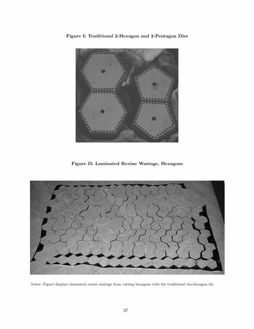
Figure I: Traditional 2-Hexagon and 2-Pentagon Dies

Figure II: Laminated Rexine Wastage, Hexagons

Notes: Figure displays laminated rexine wastage from cutting hexagons with the traditional two-hexagon die.

37

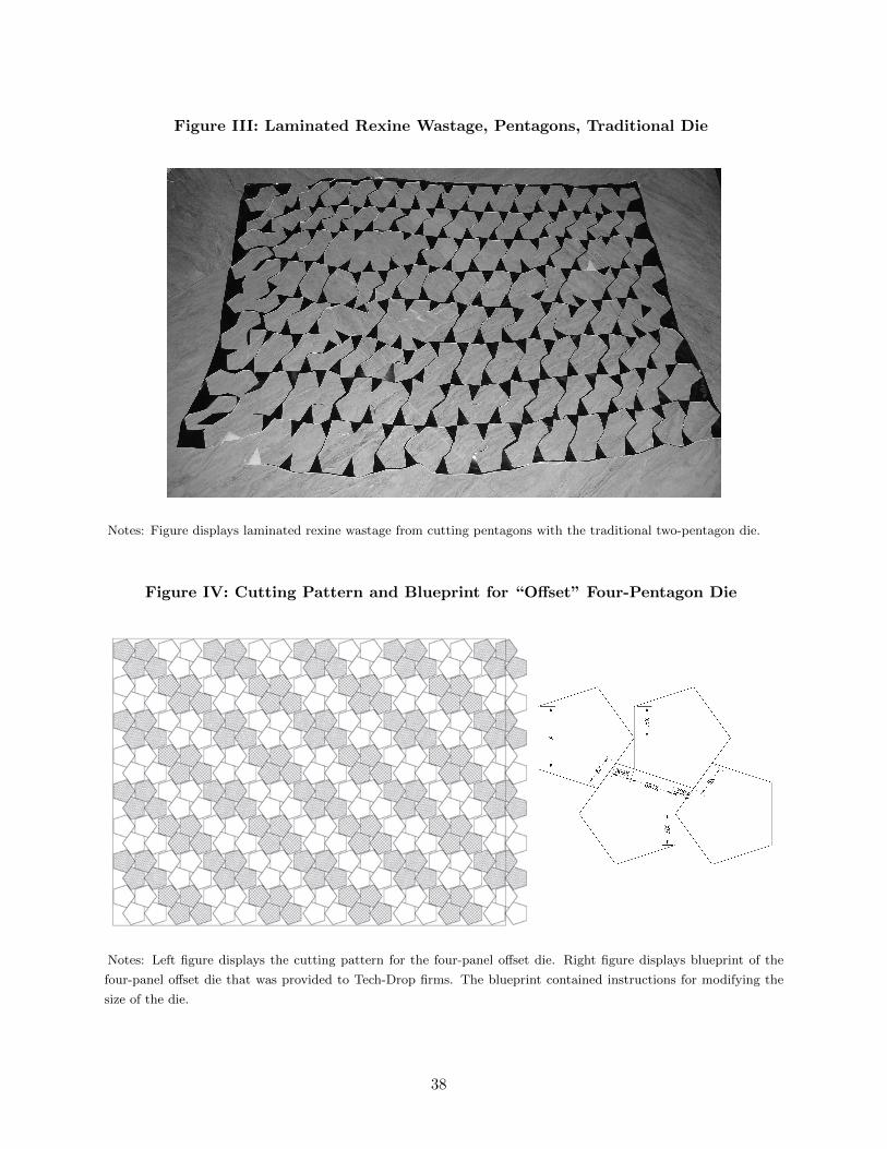
Figure III: Laminated Rexine Wastage, Pentagons, Traditional Die

Notes: Figure displays laminated rexine wastage from cutting pentagons with the traditional two-pentagon die.

Figure IV: Cutting Pattern and Blueprint for “Offset” Four-Pentagon Die

Notes: Left figure displays the cutting pattern for the four-panel offset die. Right figure displays blueprint of the

four-panel offset die that was provided to Tech-Drop firms. The blueprint contained instructions for modifying the

size of the die.

38

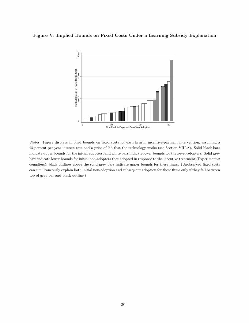
Figure V: Implied Bounds on Fixed Costs Under a Learning Subsidy Explanation

010

000

2000

030

000

Impl

ied

Bou

nds

on F

ixed

Cos

ts (

US

$)

0 10 20 30Firm Rank in Expected Benefits of Adoption

Notes: Figure displays implied bounds on fixed costs for each firm in incentive-payment intervention, assuming a

25 percent per year interest rate and a prior of 0.5 that the technology works (see Section VIII.A). Solid black bars

indicate upper bounds for the initial adopters, and white bars indicate lower bounds for the never-adopters. Solid grey

bars indicate lower bounds for initial non-adopters that adopted in response to the incentive treatment (Experiment-2

compliers); black outlines above the solid grey bars indicate upper bounds for these firms. (Unobserved fixed costs

can simultaneously explain both initial non-adoption and subsequent adoption for these firms only if they fall between

top of grey bar and black outline.)

39

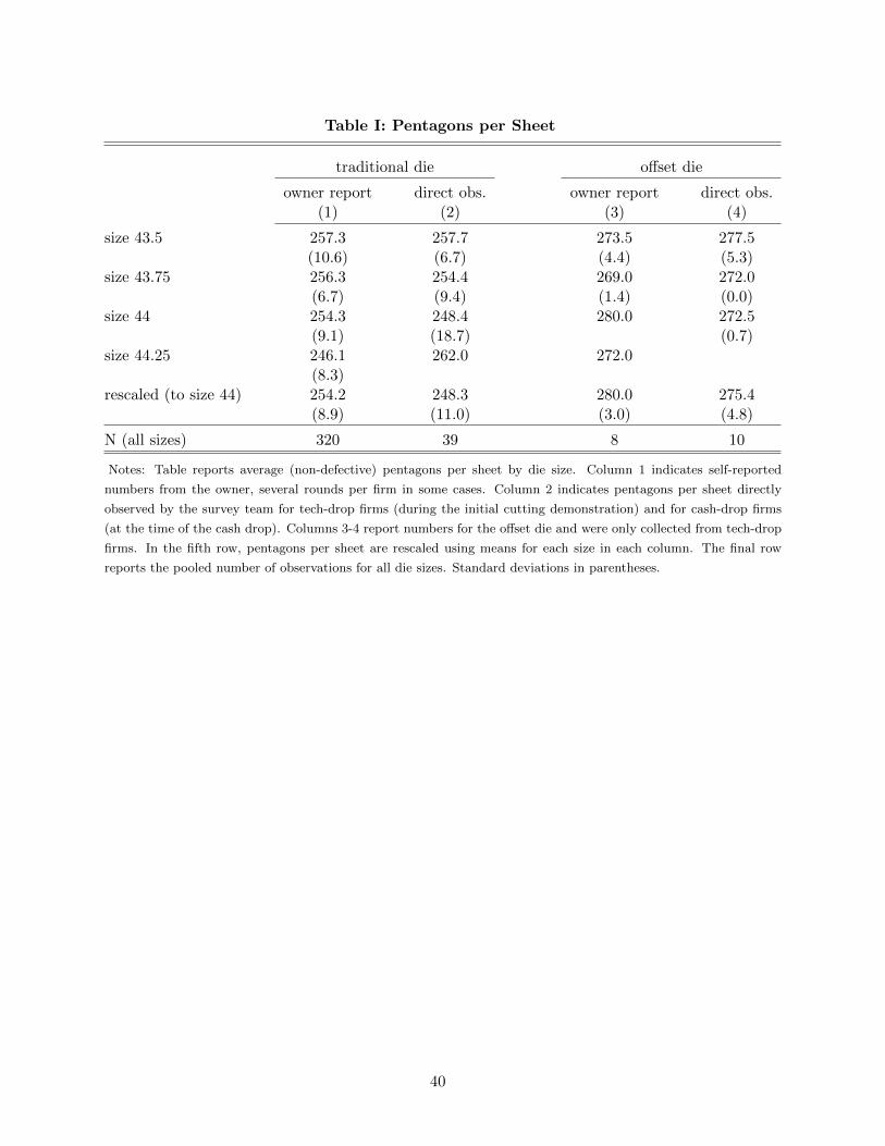
Table I: Pentagons per Sheet

traditional die offset die

owner report direct obs. owner report direct obs.(1) (2) (3) (4)

size 43.5 257.3 257.7 273.5 277.5(10.6) (6.7) (4.4) (5.3)

size 43.75 256.3 254.4 269.0 272.0(6.7) (9.4) (1.4) (0.0)

size 44 254.3 248.4 280.0 272.5(9.1) (18.7) (0.7)

size 44.25 246.1 262.0 272.0(8.3)

rescaled (to size 44) 254.2 248.3 280.0 275.4(8.9) (11.0) (3.0) (4.8)

N (all sizes) 320 39 8 10

Notes: Table reports average (non-defective) pentagons per sheet by die size. Column 1 indicates self-reported

numbers from the owner, several rounds per firm in some cases. Column 2 indicates pentagons per sheet directly

observed by the survey team for tech-drop firms (during the initial cutting demonstration) and for cash-drop firms

(at the time of the cash drop). Columns 3-4 report numbers for the offset die and were only collected from tech-drop

firms. In the fifth row, pentagons per sheet are rescaled using means for each size in each column. The final row

reports the pooled number of observations for all die sizes. Standard deviations in parentheses.

40

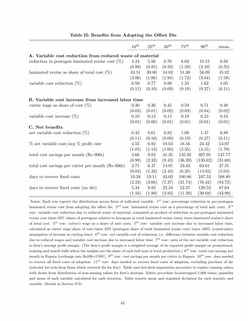
Table II: Benefits from Adopting the Offset Die

10th 25th 50th 75th 90th mean

A. Variable cost reduction from reduced waste of materialreduction in pentagon laminated rexine cost (%) 4.24 5.56 6.76 8.02 10.15 6.93

(0.99) (0.85) (0.59) (1.59) (2.10) (0.70)laminated rexine as share of total cost (%) 34.51 39.80 44.83 51.30 56.09 45.82

(3.06) (1.86) (1.94) (1.72) (3.84) (1.58)variable cost reduction (%) 0.59 0.77 0.98 1.24 1.62 1.05

(0.11) (0.10) (0.09) (0.19) (0.27) (0.11)

B. Variable cost increase from increased labor timecutter wage as share of cost (%) 0.30 0.36 0.45 0.59 0.71 0.48

(0.03) (0.01) (0.02) (0.03) (0.04) (0.02)variable cost increase (%) 0.10 0.12 0.15 0.19 0.23 0.16

(0.01) (0.00) (0.01) (0.01) (0.01) (0.01)C. Net benefitsnet variable cost reduction (%) 0.42 0.61 0.82 1.09 1.47 0.89

(0.11) (0.10) (0.09) (0.19) (0.27) (0.11)% net variable cost/avg % profit rate 4.55 6.82 10.63 16.56 24.42 13.07

(1.05) (1.13) (1.60) (2.35) (4.15) (1.79)total cost savings per month (Rs 000s) 3.66 9.82 41.35 135.92 397.95 137.77

(0.99) (2.33) (9.43) (36.39) (130.62) (31.68)total cost savings per cutter per month (Rs 000s) 2.75 6.47 14.91 33.83 63.61 27.31

(0.83) (1.33) (2.43) (6.28) (14.02) (5.04)days to recover fixed costs 10.28 19.11 43.03 100.86 247.53 168.80

(2.23) (3.66) (7.37) (21.74) (76.42) (84.72)days to recover fixed costs (no die) 5.34 9.92 22.34 52.37 128.53 87.64

(1.16) (1.90) (3.83) (11.29) (39.68) (43.99)

Notes: Each row reports the distribution across firms of indicated variable. 1st row: percentage reduction in per-pentagon

laminated rexine cost from adopting the offset die. 2nd row: laminated rexine cost as a percentage of total unit costs. 3rd

row: variable cost reduction due to reduced waste of material, computed as product of reduction in per-pentagon laminated

rexine cost times 33% (share of pentagons relative to hexagons in total laminated rexine costs) times laminated rexine’s share

of total cost. 4th row: cutter’s wage as a share of unit costs. 5th row: variable cost increase due to increased labor time,

calculated as cutter wage share of cost times 33% (pentagon share of total laminated rexine cost) times 100% (conservative

assumption of increase in cutting time). 6th row: net variable cost of reduction, i.e. difference between variable cost reduction

due to reduced wages and variable cost increase due to increased labor time. 7th row: ratio of the net variable cost reduction

to firm’s average profit margin. (The firm’s profit margin is a weighted average of its reported profit margin on promotional,

training and match balls where the weights are the share of each ball type in total production.) 8th row: total cost savings per

month in Rupees (exchange rate Rs100=US$1). 9th row: cost savings per month per cutter in Rupees. 10th row: days needed

to recover all fixed costs of adoption. 11th row: days needed to recover fixed costs of adoption, excluding purchase of die

(relevant for tech-drop firms which received die for free). Table uses hot-deck imputation procedure to replace missing values

with draws from distribution of non-missing values for firm’s stratum. Entire procedure bootstrapped 1,000 times; quantiles

and mean of each variable calculated for each iteration. Table reports mean and standard deviation for each statistic and

variable. Details in Section II.D.

41

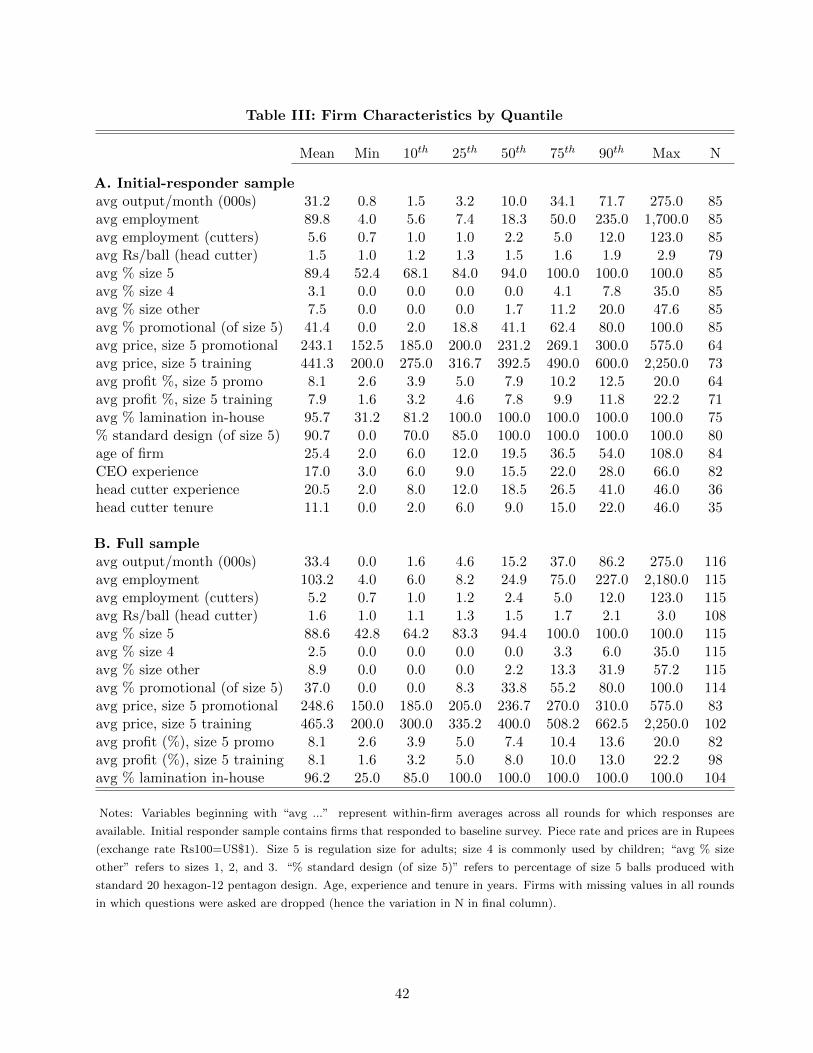
Table III: Firm Characteristics by Quantile

Mean Min 10th 25th 50th 75th 90th Max N

A. Initial-responder sampleavg output/month (000s) 31.2 0.8 1.5 3.2 10.0 34.1 71.7 275.0 85avg employment 89.8 4.0 5.6 7.4 18.3 50.0 235.0 1,700.0 85avg employment (cutters) 5.6 0.7 1.0 1.0 2.2 5.0 12.0 123.0 85avg Rs/ball (head cutter) 1.5 1.0 1.2 1.3 1.5 1.6 1.9 2.9 79avg % size 5 89.4 52.4 68.1 84.0 94.0 100.0 100.0 100.0 85avg % size 4 3.1 0.0 0.0 0.0 0.0 4.1 7.8 35.0 85avg % size other 7.5 0.0 0.0 0.0 1.7 11.2 20.0 47.6 85avg % promotional (of size 5) 41.4 0.0 2.0 18.8 41.1 62.4 80.0 100.0 85avg price, size 5 promotional 243.1 152.5 185.0 200.0 231.2 269.1 300.0 575.0 64avg price, size 5 training 441.3 200.0 275.0 316.7 392.5 490.0 600.0 2,250.0 73avg profit %, size 5 promo 8.1 2.6 3.9 5.0 7.9 10.2 12.5 20.0 64avg profit %, size 5 training 7.9 1.6 3.2 4.6 7.8 9.9 11.8 22.2 71avg % lamination in-house 95.7 31.2 81.2 100.0 100.0 100.0 100.0 100.0 75% standard design (of size 5) 90.7 0.0 70.0 85.0 100.0 100.0 100.0 100.0 80age of firm 25.4 2.0 6.0 12.0 19.5 36.5 54.0 108.0 84CEO experience 17.0 3.0 6.0 9.0 15.5 22.0 28.0 66.0 82head cutter experience 20.5 2.0 8.0 12.0 18.5 26.5 41.0 46.0 36head cutter tenure 11.1 0.0 2.0 6.0 9.0 15.0 22.0 46.0 35

B. Full sampleavg output/month (000s) 33.4 0.0 1.6 4.6 15.2 37.0 86.2 275.0 116avg employment 103.2 4.0 6.0 8.2 24.9 75.0 227.0 2,180.0 115avg employment (cutters) 5.2 0.7 1.0 1.2 2.4 5.0 12.0 123.0 115avg Rs/ball (head cutter) 1.6 1.0 1.1 1.3 1.5 1.7 2.1 3.0 108avg % size 5 88.6 42.8 64.2 83.3 94.4 100.0 100.0 100.0 115avg % size 4 2.5 0.0 0.0 0.0 0.0 3.3 6.0 35.0 115avg % size other 8.9 0.0 0.0 0.0 2.2 13.3 31.9 57.2 115avg % promotional (of size 5) 37.0 0.0 0.0 8.3 33.8 55.2 80.0 100.0 114avg price, size 5 promotional 248.6 150.0 185.0 205.0 236.7 270.0 310.0 575.0 83avg price, size 5 training 465.3 200.0 300.0 335.2 400.0 508.2 662.5 2,250.0 102avg profit (%), size 5 promo 8.1 2.6 3.9 5.0 7.4 10.4 13.6 20.0 82avg profit (%), size 5 training 8.1 1.6 3.2 5.0 8.0 10.0 13.0 22.2 98avg % lamination in-house 96.2 25.0 85.0 100.0 100.0 100.0 100.0 100.0 104

Notes: Variables beginning with “avg ...” represent within-firm averages across all rounds for which responses are

available. Initial responder sample contains firms that responded to baseline survey. Piece rate and prices are in Rupees

(exchange rate Rs100=US$1). Size 5 is regulation size for adults; size 4 is commonly used by children; “avg % size

other” refers to sizes 1, 2, and 3. “% standard design (of size 5)” refers to percentage of size 5 balls produced with

standard 20 hexagon-12 pentagon design. Age, experience and tenure in years. Firms with missing values in all rounds

in which questions were asked are dropped (hence the variation in N in final column).

42

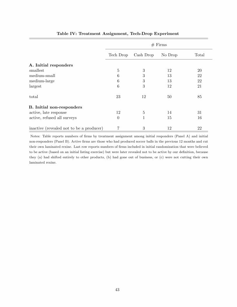
Table IV: Treatment Assignment, Tech-Drop Experiment

# Firms

Tech Drop Cash Drop No Drop Total

A. Initial responderssmallest 5 3 12 20medium-small 6 3 13 22medium-large 6 3 13 22largest 6 3 12 21

total 23 12 50 85

B. Initial non-respondersactive, late response 12 5 14 31active, refused all surveys 0 1 15 16

inactive (revealed not to be a producer) 7 3 12 22

Notes: Table reports numbers of firms by treatment assignment among initial responders (Panel A) and initial

non-responders (Panel B). Active firms are those who had produced soccer balls in the previous 12 months and cut

their own laminated rexine. Last row reports numbers of firms included in initial randomization that were believed

to be active (based on an initial listing exercise) but were later revealed not to be active by our definition, because

they (a) had shifted entirely to other products, (b) had gone out of business, or (c) were not cutting their own

laminated rexine.

43

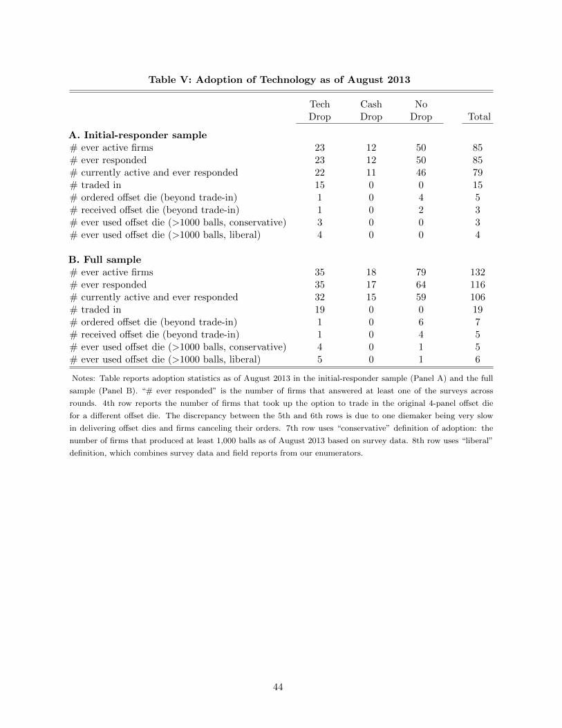
Table V: Adoption of Technology as of August 2013

TechDrop

CashDrop

NoDrop Total

A. Initial-responder sample# ever active firms 23 12 50 85# ever responded 23 12 50 85# currently active and ever responded 22 11 46 79# traded in 15 0 0 15# ordered offset die (beyond trade-in) 1 0 4 5# received offset die (beyond trade-in) 1 0 2 3# ever used offset die (>1000 balls, conservative) 3 0 0 3# ever used offset die (>1000 balls, liberal) 4 0 0 4

B. Full sample# ever active firms 35 18 79 132# ever responded 35 17 64 116# currently active and ever responded 32 15 59 106# traded in 19 0 0 19# ordered offset die (beyond trade-in) 1 0 6 7# received offset die (beyond trade-in) 1 0 4 5# ever used offset die (>1000 balls, conservative) 4 0 1 5# ever used offset die (>1000 balls, liberal) 5 0 1 6

Notes: Table reports adoption statistics as of August 2013 in the initial-responder sample (Panel A) and the full

sample (Panel B). “# ever responded” is the number of firms that answered at least one of the surveys across

rounds. 4th row reports the number of firms that took up the option to trade in the original 4-panel offset die

for a different offset die. The discrepancy between the 5th and 6th rows is due to one diemaker being very slow

in delivering offset dies and firms canceling their orders. 7th row uses “conservative” definition of adoption: the

number of firms that produced at least 1,000 balls as of August 2013 based on survey data. 8th row uses “liberal”

definition, which combines survey data and field reports from our enumerators.

44

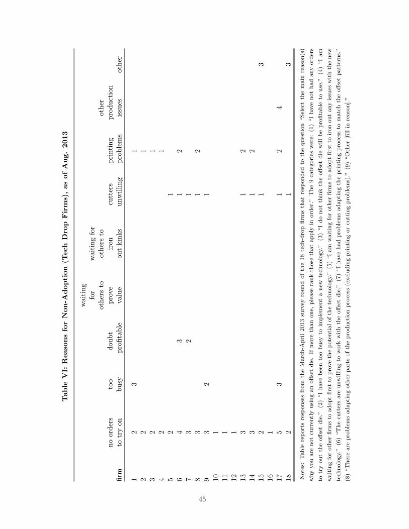
Tab

leV

I:R

easo

ns

for

Non

-Ad

op

tion

(Tech

Dro

pF

irm

s),

as

of

Au

g.

2013

firm

no

ord

ers

totr

yon

too

bu

syd

oub

tp

rofi

tab

le

wai

tin

gfo

rot

her

sto

pro

veva

lue

wai

tin

gfo

rot

her

sto

iron

out

kin

ks

cutt

ers

unw

illi

ng

pri

nti

ng

pro

ble

ms

oth

erp

rod

uct

ion

issu

esot

her

12

31

22

13

21

42

15

21

64

31

27

32

18

31

29

32

110

111

112

113

31

214

31

215

21

316

117

53

12

418

21

3

Note

s:T

able

rep

ort

sre

sponse

sfr

om

the

Marc

h-A

pri

l2013

surv

eyro

und

of

the

18

tech

-dro

pfirm

sth

at

resp

onded

toth

eques

tion

“Sel

ect

the

main

reaso

n(s

)

why

you

are

not

curr

entl

yusi

ng

an

off

set

die

.If

more

than

one,

ple

ase

rank

those

that

apply

inord

er.”

The

9ca

tegori

esw

ere:

(1)

“I

hav

enot

had

any

ord

ers

totr

yout

the

off

set

die

.”(2

)“I

hav

eb

een

too

busy

toim

ple

men

ta

new

tech

nolo

gy.

”(3

)“I

do

not

thin

kth

eoff

set

die

will

be

pro

fita

ble

touse

.”(4

)“I

am

wait

ing

for

oth

erfirm

sto

adopt

firs

tto

pro

ve

the

pote

nti

al

of

the

tech

nolo

gy.

”(5

)“I

am

wait

ing

for

oth

erfirm

sto

adopt

firs

tto

iron

out

any

issu

esw

ith

the

new

tech

nolo

gy.

”(6

)“T

he

cutt

ers

are

unw

illing

tow

ork

wit

hth

eoff

set

die

.”(7

)“I

hav

ehad

pro

ble

ms

adapti

ng

the

pri

nti

ng

pro

cess

tom

atc

hth

eoff

set

patt

erns.

”

(8)

“T

her

eare

pro

ble

ms

adapti

ng

oth

erpart

sof

the

pro

duct

ion

pro

cess

(excl

udin

gpri

nti

ng

or

cutt

ing

pro

ble

ms)

.”(9

)“O

ther

[fill

inre

aso

n].”

45

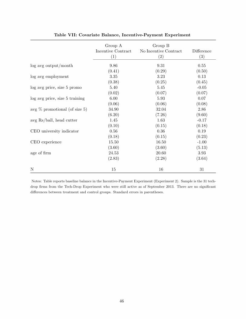
Table VII: Covariate Balance, Incentive-Payment Experiment

Group AIncentive Contract

(1)

Group BNo Incentive Contract

(2)Difference

(3)

log avg output/month 9.86 9.31 0.55(0.41) (0.29) (0.50)

log avg employment 3.35 3.23 0.13(0.38) (0.25) (0.45)

log avg price, size 5 promo 5.40 5.45 -0.05(0.02) (0.07) (0.07)

log avg price, size 5 training 6.00 5.93 0.07(0.06) (0.06) (0.08)

avg % promotional (of size 5) 34.90 32.04 2.86(6.20) (7.26) (9.60)

avg Rs/ball, head cutter 1.45 1.63 -0.17(0.10) (0.15) (0.18)

CEO university indicator 0.56 0.36 0.19(0.18) (0.15) (0.23)

CEO experience 15.50 16.50 -1.00(3.60) (3.60) (5.13)

age of firm 24.53 20.60 3.93(2.83) (2.28) (3.64)

N 15 16 31

Notes: Table reports baseline balance in the Incentive-Payment Experiment (Experiment 2). Sample is the 31 tech-

drop firms from the Tech-Drop Experiment who were still active as of September 2013. There are no significant

differences between treatment and control groups. Standard errors in parentheses.

46

Table VIII: Incentive-Payment Experiment (Liberal Adoption Measure)

Dep. var.: adoption (>1,000 balls, liberal measure)

FirstStage OLS

ReducedForm (ITT)

IV(TOT)

(1) (2) (3) (4)

A. Short-Run (as of Round 6)received treatment 0.48*** 0.48***

(0.15) (0.15)assigned to group A 0.68*** 0.32**

(0.12) (0.12)

stratum dummies Y Y Y Ymean of group B (control group) 0.19 0.19 0.19R-squared 0.57 0.69 0.60 0.69N 31 31 31 31

B. Medium-Run (as of Round 7)received treatment 0.41** 0.37**

(0.16) (0.17)assigned to group A 0.72*** 0.27*

(0.12) (0.14)

stratum dummies Y Y Y Ymean of group B (control group) 0.27 0.27 0.27R-squared 0.60 0.61 0.52 0.61N 29 29 29 29

Notes: Table reports results of incentive-payment experiment on adoption rates using the liberal definition of

adoption. Panel A reports short-run results as of Round 6 (Jan.-March 2014). Panel B reports medium-run results

as of Round 7 (Oct.-Dec. 2014). The dependent variable in Column 1 is an indicator variable for whether the

firm received treatment. Two firms exited between Rounds 6 and 7. All regressions include stratum dummies, and

report robust standard errors. Significance: * 0.10, ** 0.05; *** 0.01.

47

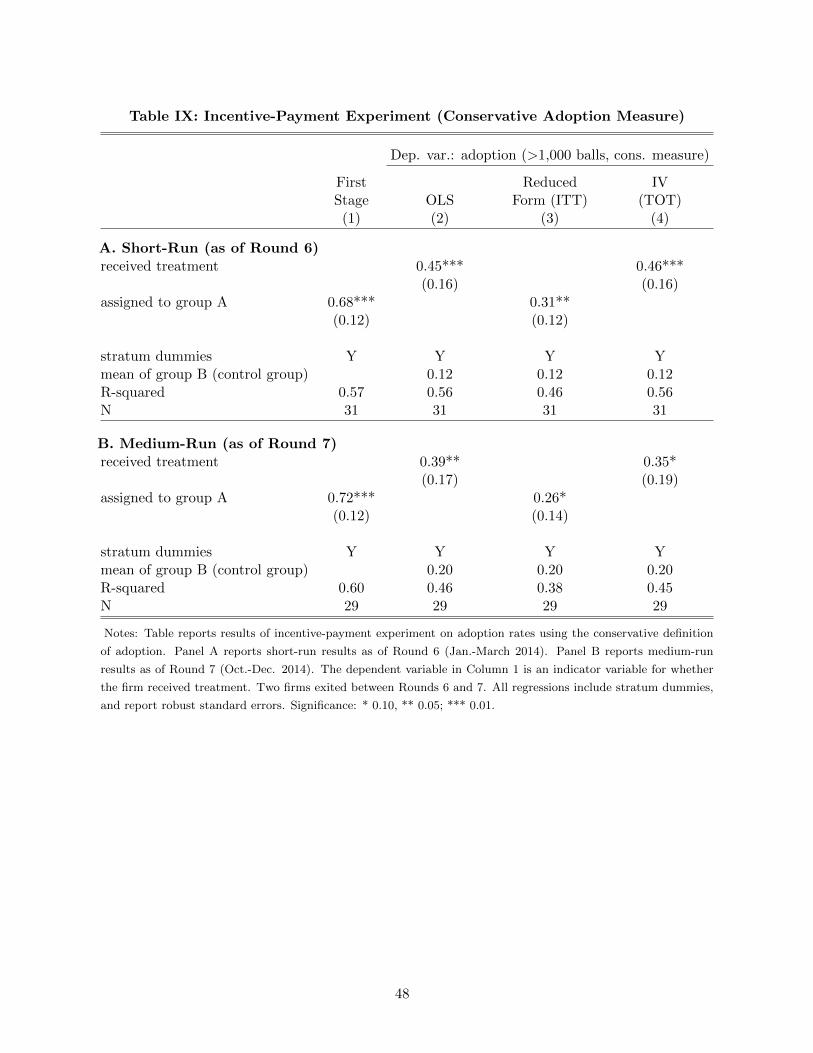
Table IX: Incentive-Payment Experiment (Conservative Adoption Measure)

Dep. var.: adoption (>1,000 balls, cons. measure)

FirstStage OLS

ReducedForm (ITT)

IV(TOT)

(1) (2) (3) (4)

A. Short-Run (as of Round 6)received treatment 0.45*** 0.46***

(0.16) (0.16)assigned to group A 0.68*** 0.31**

(0.12) (0.12)

stratum dummies Y Y Y Ymean of group B (control group) 0.12 0.12 0.12R-squared 0.57 0.56 0.46 0.56N 31 31 31 31

B. Medium-Run (as of Round 7)received treatment 0.39** 0.35*

(0.17) (0.19)assigned to group A 0.72*** 0.26*

(0.12) (0.14)

stratum dummies Y Y Y Ymean of group B (control group) 0.20 0.20 0.20R-squared 0.60 0.46 0.38 0.45N 29 29 29 29

Notes: Table reports results of incentive-payment experiment on adoption rates using the conservative definition

of adoption. Panel A reports short-run results as of Round 6 (Jan.-March 2014). Panel B reports medium-run

results as of Round 7 (Oct.-Dec. 2014). The dependent variable in Column 1 is an indicator variable for whether

the firm received treatment. Two firms exited between Rounds 6 and 7. All regressions include stratum dummies,

and report robust standard errors. Significance: * 0.10, ** 0.05; *** 0.01.

48

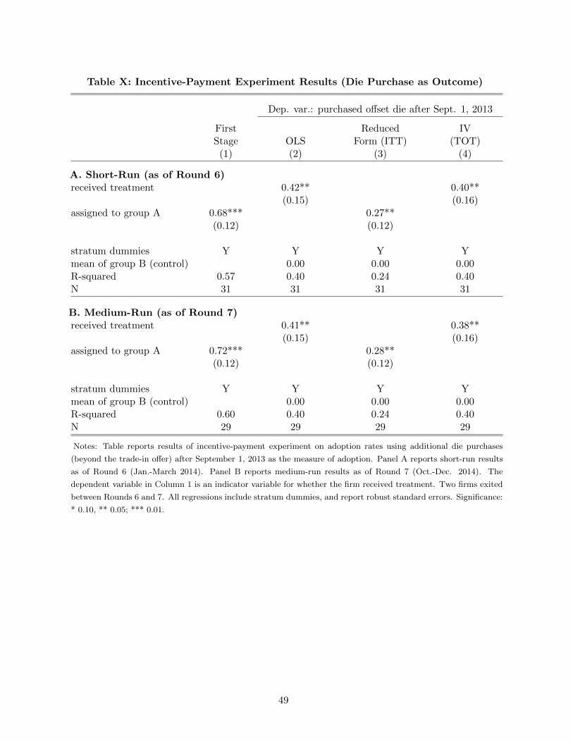
Table X: Incentive-Payment Experiment Results (Die Purchase as Outcome)

Dep. var.: purchased offset die after Sept. 1, 2013

FirstStage OLS

ReducedForm (ITT)

IV(TOT)

(1) (2) (3) (4)

A. Short-Run (as of Round 6)received treatment 0.42** 0.40**

(0.15) (0.16)assigned to group A 0.68*** 0.27**

(0.12) (0.12)

stratum dummies Y Y Y Ymean of group B (control) 0.00 0.00 0.00R-squared 0.57 0.40 0.24 0.40N 31 31 31 31

B. Medium-Run (as of Round 7)received treatment 0.41** 0.38**

(0.15) (0.16)assigned to group A 0.72*** 0.28**

(0.12) (0.12)

stratum dummies Y Y Y Ymean of group B (control) 0.00 0.00 0.00R-squared 0.60 0.40 0.24 0.40N 29 29 29 29

Notes: Table reports results of incentive-payment experiment on adoption rates using additional die purchases

(beyond the trade-in offer) after September 1, 2013 as the measure of adoption. Panel A reports short-run results

as of Round 6 (Jan.-March 2014). Panel B reports medium-run results as of Round 7 (Oct.-Dec. 2014). The

dependent variable in Column 1 is an indicator variable for whether the firm received treatment. Two firms exited

between Rounds 6 and 7. All regressions include stratum dummies, and report robust standard errors. Significance:

* 0.10, ** 0.05; *** 0.01.

49

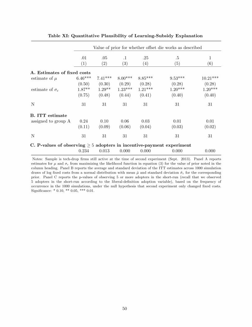
Table XI: Quantitative Plausibility of Learning-Subsidy Explanation

Value of prior for whether offset die works as described

.01 .05 .1 .25 .5 1(1) (2) (3) (4) (5) (6)

A. Estimates of fixed costsestimate of µ 6.46*** 7.41*** 8.00*** 8.85*** 9.53*** 10.21***

(0.50) (0.30) (0.29) (0.28) (0.28) (0.28)estimate of σε 1.87** 1.29** 1.23*** 1.21*** 1.20*** 1.20***

(0.75) (0.48) (0.44) (0.41) (0.40) (0.40)

N 31 31 31 31 31 31

B. ITT estimateassigned to group A 0.24 0.10 0.06 0.03 0.01 0.01

(0.11) (0.09) (0.06) (0.04) (0.03) (0.02)

N 31 31 31 31 31 31

C. P-values of observing ≥ 5 adopters in incentive-payment experiment0.234 0.013 0.000 0.000 0.000 0.000

Notes: Sample is tech-drop firms still active at the time of second experiment (Sept. 2013). Panel A reportsestimates for µ and σε from maximizing the likelihood function in equation (3) for the value of prior noted in thecolumn heading. Panel B reports the average and standard deviation of the ITT estimates across 1000 simulationdraws of log fixed costs from a normal distribution with mean µ̂ and standard deviation σ̂ε for the correspondingprior. Panel C reports the p-values of observing 5 or more adopters in the short-run (recall that we observed5 adopters in the short-run according to the liberal-definition adoption variable), based on the frequency ofoccurrence in the 1000 simulations, under the null hypothesis that second experiment only changed fixed costs.Significance: * 0.10, ** 0.05, *** 0.01.

50