HUNGARIAN JOURNAL OF INDUSTRY AND CHEMISTRY

Vol. 43(1) pp. 33–38 (2015) hjic.mk.uni-pannon.hu

DOI: 10.1515/hjic-2015-0006

ORGANISATION OF THE ANALYTICAL, STOICHIOMETRIC, AND THERMODYNAMIC INFORMATION FOR WATER CHEMISTRY CALCULATIONS

RITA FÖLDÉNYI* AND AURÉL MARTON

Department of Environmental Science, University of Pannonia, Egyetem u. 10., Veszprém, 8200, HUNGARY

A common feature of the chemical processes of the hydrosphere and water treatment plants is that essentially the same types of chemical equilibrium reactions occur in both fields. These equilibria could be acid/base, complexation, redox, precipitation, and interfacial processes. Since these reactions may also occur in combination, the aqueous environments are unavoidably multispecies systems. Due to multiple equilibria, the state of aggregation, the state of oxidation, as well as the electric charge of the species may change dramatically. Calculation of the equilibrium concentration of the species is facilitated by the availability of analytical, stoichiometric, and thermodynamic information that are consistently organised into an ASTI matrix. The matrix makes it possible to apply a uniform algebraic treatment for all occurring equilibria even, if later on, further reactions have to be included in the chemical model. The use of the ASTI matrix enables us to set up the necessary mass balance equations and equilibrium relationships, which together form a non-linear system of equations (NLSE). The goal of our paper is to show that the use of the ASTI matrix approach in cooperation with the powerful engineering calculation software, MATHCAD14, results in fast and easy handling of the NLSE-s and, consequently, the calculations of speciation in aqueous systems. The paper demonstrates the method of application in three examples: the calculation of the pH dependence of the solubility of calcite in closed and open systems, the calculation of the pH and pε in a system where acid/base reactions, complexation equilibria, and redox equilibria occur, and a study of adsorption of lead ions on aluminium oxide.

Keywords: multiple solution equilibria, ASTI matrix method, solubility of calcite, redox calculation, adsorption of lead

1. Introduction

Information on the speciation profile of aqueous systems is of primary importance in many fields of chemistry. The usual acid/base, complexation, redox, precipitation, and interfacial reactions may occur simultaneously leading to the formation of a large number of species in both natural and artificial aquatic systems. Contemporary numerical and graphical treatments of aqueous equilibria were presented in seminal publications in the fields of environmental engineering [1], natural aquatic systems [2–7] and geochemistry [8, 9]. An important aspect of the recent approaches is the systematic organisation of the analytical, stoichiometric, and thermodynamic information relevant to the studied system. The input of structured information became particularly indispensable in the use of the modern computer programs dedicated to chemical equilibrium modelling: MINEQL [10], MINEQL+ [11], MINTEQA [12], PHREEQC [13], and WHAM [14], to name a few.

*Correspondence: foldenyi@almos.uni-pannon.hu

2. Methods

2.1. Organisation of Information into the ASTI Matrix

In order to collect and organise data for the equilibrium calculations a strict distinction has to be made between the terms: reagent, reactions, species and components. Under laboratory conditions, reagents (denoted hereafter by A) are simply those chemicals that are present at the beginning of reactions. Each reagent is characterised by its analytical molar concentration (c in mol dm-3 or M). Under environmental conditions, we have to assume the presence of a ‘contaminating’ compound of reagents: e.g. acid rain forms as a result of due to the presence of nitric acid in rainwater.

When reagents are mixed, several reactions may take place (the total number of reactions is denoted by R). For each reaction, the relevant equilibrium constant (K) refers to the correct stoichiometry of the reaction, such as

H2CO3 ⇄ HCO3- + H+, K1 = 10-6.35 (1)

HCO3- ⇄ CO3

2- + H+, K2 = 10-10.33 (2)

FÖLDÉNYI AND MARTON

Hungarian Journal of Industry and Chemistry

34

where the K values are given for a specified temperature (25 ºC), pressure (101.3 kPa), and ionic strength (0.1 M).

The considered reactions or chemical models generate a large number of chemical particles with appreciable stabilities. This set of entities is called species (the number of species is denoted by S). The smallest subset of selected species that enable us to describe the formation of all the other species of the system are called components (their number is denoted by C). In order to meet the requirements of the Gibbs phase rule [15], the needed number of components has to be calculated from the relationship C = S - R. If there are 6 reactions and 10 species then from the list of species four species have to be selected as component C = 4. The concept of this component is the “key and door” to the organisation of the database and, consequently, to equilibrium calculations.

In principle, any subset of the species can be selected (promoted) as a component, but chemical considerations dictate some rules that have to be kept in mind:

1. H2O and H+ have to always be selected as components,

2. Species with fixed activities whose concentrations do not change during the reactions have to be selected as components too; such species are the solvent (H2O), solid phases (e.g. CaCO3), and gases of known pressure (e.g. atmospheric CO2, p = 10-3.5 atm), and

3. Species that are presumably present in dominant concentrations will also be selected as components.

After selecting the components, the formation reactions for the rest of the species have to be written up in terms of these components. The equilibrium (formation) constant of the species is calculated by Hess’s law using algebraic manipulation of the reactions, in such a way, to obtain the target reaction. The left-hand side of the target reaction only contains components and the right-hand side only displays the species e.g.: if in the studied system CO3

2- is selected as a component (besides H2O and H+) then by using Eqs.(1) and (2), the formation of the HCO3

- and H2CO3 species should be given as:

CO32- + H+ ⇄ HCO3

- , (K2)-1 (3)

CO32- + 2H+ ⇄ H2CO3 . (K1·K2)-1 (4)

When the formation of all the (S - C) species is expressed in this way then the stoichiometric relationship between the components and species is revealed. In addition to this, the stoichiometric connection between the components and reagents has to be established too. This can be done by synthesising the reagents through the reaction of the components, just like in the case of species, but now only the stoichiometric coefficients are relevant.

The above procedure highlights the central role of the component and allows us to arrange the available analytical, stoichiometric and thermodynamic

information into a coherent matrix abbreviated hereafter as the ASTI matrix. The columns and rows of the matrix list the C number of components and all the S number of species, respectively. The elements of the matrix are filled with the respective stoichiometric coefficients (including zeros too). Analytical concentrations (c) and the equilibrium constants (K) are introduced into this matrix as shown in the examples discussed below.

For the calculation of the unknown concentration of S species, we need the S stoichiometrically independent equation. The main purpose of our effort to develop the ASTI matrix is to draw up the required S equations. Based on the columns and rows matrix two types of equations can be drawn up. The mass balance equations (MB) are based on the columns of the ASTI matrix and are drawn up usually for all the C components (in exceptional cases, not all the MB equations are needed, see Example 1. below). The MB equation is, in fact, an additive relationship showing the weighed concentration sum of all species containing the particular component. The weighing factors are the respective stoichiometric coefficients. The other type of equations, based on the ASTI matrix, are the equilibrium relationships (ER). This multiplicative type of equations are drawn up on the basis of the rows of the species. The ER gives the equilibrium concentration of the (S - C) species expressed as a product of the concentration of all the C components raised to the power of the stoichiometric coefficients (which could be zeros too). Consequently, the ER-s expresses the concentration of the species in terms of the concentration of the components. It is worth noting, that a different choice of components yields different MB equations and ER (a further indication of the importance of the choice of component in the equilibrium calculation). The application of these principles will be shown in the examples below. The mass balance equations together with the equilibrium relationships form a (usually) non-linear system of equations (NLSE) for calculating the concentration of all the S species.

2.2. Solving the Non-Linear System of Equations (NLSE) using MATHCAD

MATHCAD 14 (PTC. Inc.) is a versatile and powerful engineering calculation software. It works seamlessly with numbers, units, equations, texts, and graphs. After giving the required K, analytical concentration data, and assigning initial values for the unknown variables, the S number of NLSE is introduced on the screen between the Given and Find commands. MATHCAD then rapidly solves the NLSE by using the iterative Levenberg - Marquardt algorithm [16]. For example, the solution of the NLSE with ten unknowns takes only a couple of seconds.

To assign a good guess for ten variables is rather cumbersome; therefore, the algebraic reduction of the number of unknowns is desirable. This can be done by substituting the equilibrium relationships into the mass balance equations, which reduces the number of variables against the number of components (C < S). In

ORGANISATION OF THE ANALYTICAL, STOICHIMETRIC, AND THERMODYNAMIC INFORMATION

43(1) pp. 33–38 (2015) DOI: 10.1515/hjic-2015-0006

35

this case, the solution of the C number of NLSE (instead of the S) returns the equilibrium concentration of the components, which are then substituted into the applicable ER to obtain the concentration of the (S - C) species. In addition to this algebraic method of the reduction of variables, chemical considerations may also be applied to reduce the number of species. Chemical background information often suggests that certain species of the system are present in minor concentrations only. These terms may then be safely omitted from the additive type of MB equations and neglected from the set of ER-s. This principle works for the opposite case too. Sometimes it is desirable to improve the original chemical model by including further equilibria. This can be done seamlessly if the new equilibria are expressed also in terms of the components and the ASTI matrix is augmented by the required new data.

The above considerations clearly highlight the appreciable advantage of using the ASTI matrices in association with MATHCAD. The ASTI matrix can be decomposed and treated by the well known methods of matrix algebra. Here; however, we like to keep chemistry in focus, so the matrix algebraic solution is not treated here explicitly, because its elegant and concise formalism conceals chemical insights.

3. Simulation Results

3.1. Calculation of the pH Dependence of the Solubility of Calcite in Open and Closed Systems (Example 1)

The solubility of CaCO3(s) in water is calculated as a function of pH for an open and a closed system. The open system is exposed to the atmosphere where pCO2 is 10-3.5 atm, where the exchange of CO2 molecules between the solution and gas phases is allowed. Considering the similarities between the two systems, and for brevity, the process leading to the ASTI matrix and the NLSE is shown only for the open system, while the results are presented for both systems. In the open system, we have three species whose equilibrium concentrations (activity, a) are known (H2O(l) with a = 1, CaCO3(s) with a = 1, pCO2 = 10-3.5 atm) so, according to rules of selection from above, they have to be selected as components. The details of the procedure are shown below:

Reagents, A=3: H2O(l) a = 1, CaCO3(s) a = 1, pCO2= 10-3.5 Reactions, R = 5:

H2O ⇄ H+ + OH- Kv = 10-14 Ca2+ + CO3

2- ⇄ CaCO3(s) Ks = 108.35 CO2(g) + H2O ⇄ H2CO3

* KH = 10-1.5 CO3

2- + H+ ⇄ HCO3- K1 = 1010.3

HCO3- + H+ ⇄ H2CO3

* K2 = 106.3 Species, S = 9: H2O, H+, OH-, CO3

2-, HCO3-, H2CO3

*, CO2(g), CaCO3(s), Ca2+ Components, C = S – R = 4 H2O, H+, CaCO3(s), CO2(g) ASTI matrix

S/C H2O H+ CO2(g) CaCO3(s) K (logK)

H2O 1

H+ 1

CO2(g) 1

CaCO3(s) 1

OH- 1 -1 Kw (-14)

Ca2+ 2 -1 1 Ks-1·KH

-1·K1·K2 (9.8)

H2CO3* 1 1 KH (-1.5)

HCO3- 1 -1 1 KH·K2

-1 (-7.8)

CO32- 1 -2 1 KH·(K1·K2)-1 (-18.1)

A/TOT M

a(H2O) 1 1

a(CaCO3(s)) 1 1

pCO2(g) 1 10-3.5

Mass balance equations, MB TOTH = [H+] - [OH-] + 2[Ca2+] - [HCO3

-] - 2[CO32-] = 0

Equilibrium relationships, ER [OH-] = Kv·[H+]-1 [Ca2+] = Ks

-1·KH-1·K1·K2 ·(pCO2)-1·[H+]2

[H2CO3*] = KH· pCO2 [HCO3

-] = KH·K2-1·pCO2·[H+]-1

[CO32-] = KH·(K1·K2)-1·pCO2·[H+]-2

The required six equations (MB + ER) are therefore available for the calculation of the six unknown concentrations (H+, OH-, CO3

2-, HCO3-,

H2CO3*, and Ca2+). The NLSE was solved by

MATHCAD and the results are shown in Table 1. For the closed system, the ASTI matrix can be

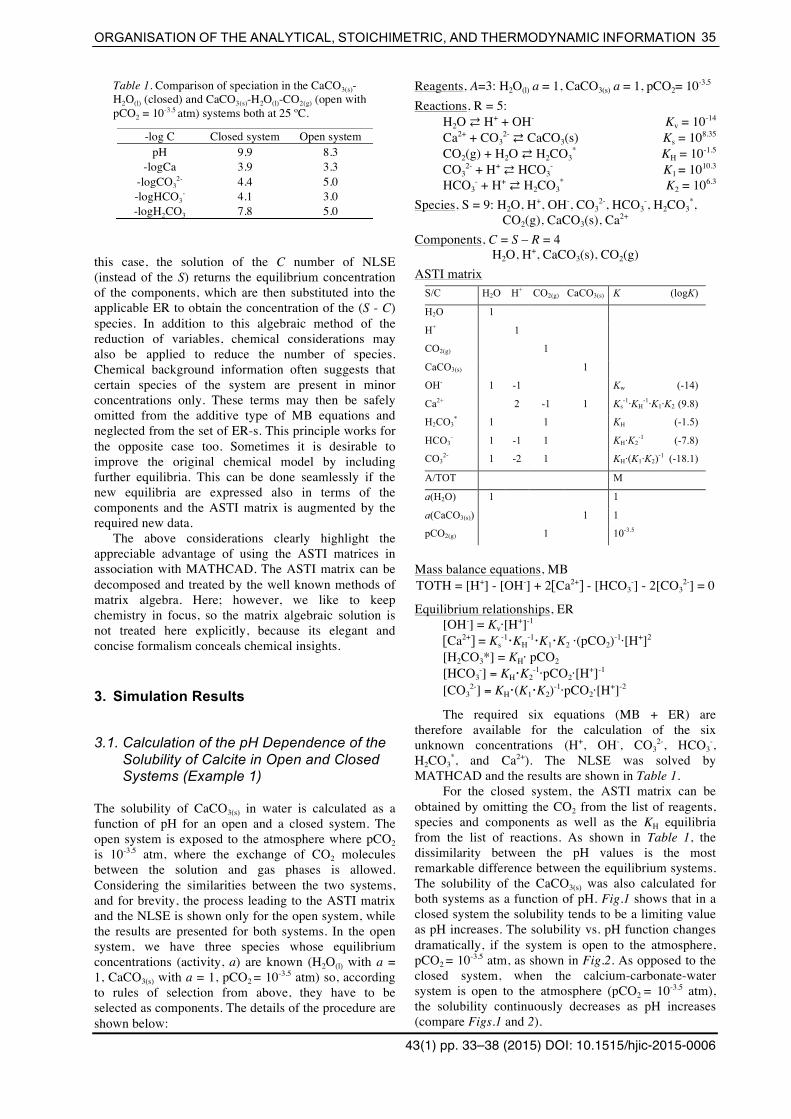
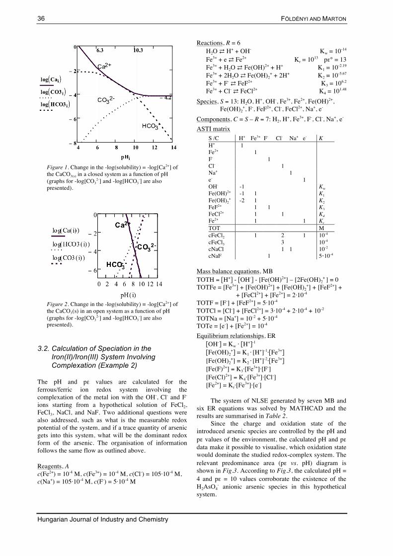
obtained by omitting the CO2 from the list of reagents, species and components as well as the KH equilibria from the list of reactions. As shown in Table 1, the dissimilarity between the pH values is the most remarkable difference between the equilibrium systems. The solubility of the CaCO3(s) was also calculated for both systems as a function of pH. Fig.1 shows that in a closed system the solubility tends to be a limiting value as pH increases. The solubility vs. pH function changes dramatically, if the system is open to the atmosphere, pCO2 = 10-3.5 atm, as shown in Fig.2. As opposed to the closed system, when the calcium-carbonate-water system is open to the atmosphere (pCO2 = 10-3.5 atm), the solubility continuously decreases as pH increases (compare Figs.1 and 2).

Table 1. Comparison of speciation in the CaCO3(s)-H2O(l) (closed) and CaCO3(s)-H2O(l)-CO2(g) (open with pCO2 = 10-3.5 atm) systems both at 25 ºC.

-log C Closed system Open system pH 9.9 8.3

-logCa 3.9 3.3 -logCO3

2- 4.4 5.0 -logHCO3

- 4.1 3.0 -logH2CO3 7.8 5.0

FÖLDÉNYI AND MARTON

Hungarian Journal of Industry and Chemistry

36

3.2. Calculation of Speciation in the Iron(II)/Iron(III) System Involving Complexation (Example 2)

The pH and pε values are calculated for the ferrous/ferric ion redox system involving the complexation of the metal ion with the OH-, Cl- and F- ions starting from a hypothetical solution of FeCl2, FeCl3, NaCl, and NaF. Two additional questions were also addressed, such as what is the measurable redox potential of the system, and if a trace quantity of arsenic gets into this system, what will be the dominant redox form of the arsenic. The organisation of information follows the same flow as outlined above.

Reagents, A c(Fe2+) = 10-4 M, c(Fe3+) = 10-4 M, c(Cl-) = 105·10-4 M, c(Na+) = 105·10-4 M, c(F-) = 5·10-4 M

Reactions, R = 6 H2O ⇄ H+ + OH- Kw = 10-14 Fe3+ + e ⇄ Fe2+ Kr = 1013 pε° = 13 Fe3+ + H2O ⇄ Fe(OH)2+ + H+ K1 = 10-2.19 Fe3+ + 2H2O ⇄!Fe(OH)2

+ + 2H+ K2 = 10-5.67 Fe3+ + F- ⇄ FeF2+ K3 = 106.2 Fe3+ + Cl- ⇄ FeCl2+ K4 = 101.48

Species, S = 13: H2O, H+, OH-, Fe3+, Fe2+, Fe(OH)2+, Fe(OH)2

+, F-, FeF2+, Cl-, FeCl2+, Na+, e- Components, C = S – R = 7: H2, H+, Fe3+, F-, Cl-, Na+, e- ASTI matrix

S /C H+ Fe3+ F- Cl- Na+ e- K H+ 1 Fe2+ 1 F- 1 Cl- 1 Na+ 1 e- 1 OH- -1 Kw Fe(OH)2+ -1 1 K1 Fe(OH)2

+ -2 1 K2 FeF2+ 1 1 K3 FeCl2+ 1 1 K4 Fe2+ 1 1 Kr TOT M cFeCl2 1 2 1 10-4 cFeCl3 3 10-4 cNaCl 1 1 10-2 cNaF 1 5·10-4

Mass balance equations, MB TOTH = [H+] - [OH-] - [Fe(OH)2+] – [2Fe(OH)2

+ ] = 0 TOTFe = [Fe3+] + [Fe(OH)2+] + [Fe(OH)2

+] + [FeF2+] + + [FeCl2+] + [Fe2+] = 2·10-4 TOTF = [F-] + [FeF2+] = 5·10-4

TOTCl = [Cl-] + [FeCl2+] = 3·10-4 + 2·10-4 + 10-2 TOTNa = [Na+] = 10-2 + 5·10-4 TOTe = [e-] + [Fe2+] = 10-4 Equilibrium relationships, ER

[OH-] = Kw ⋅ [H+]-1 [Fe(OH)2

+] = K1 ⋅ [H+]-1⋅[Fe3+] [Fe(OH)2

+] = K2 ⋅ [H+]-2⋅[Fe3+] [Fe(F)2+] = K3·[Fe3+]·[F-] [Fe(Cl)2+] = K4·[Fe3+]·[Cl-] [Fe2+] = Kr·[Fe3+]·[e-]

The system of NLSE generated by seven MB and six ER equations was solved by MATHCAD and the results are summarised in Table 2.

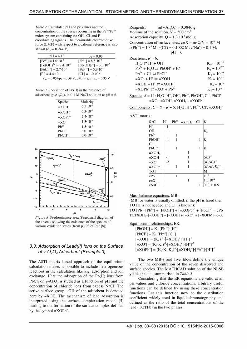
Since the charge and oxidation state of the introduced arsenic species are controlled by the pH and pε values of the environment, the calculated pH and pε data make it possible to visualise, which oxidation state would dominate the studied redox-complex system. The relevant predominance area (pε vs. pH) diagram is shown in Fig.3. According to Fig.3, the calculated pH = 4 and pε = 10 values corroborate the existence of the H2AsO4

- anionic arsenic species in this hypothetical system.

Figure 2. Change in the -log(solubility) = -log[Ca2+] of the CaCO3(s) in an open system as a function of pH (graphs for -log[CO3

2-] and -log[HCO3-] are also

presented).

Figure 1. Change in the -log(solubility) = -log[Ca2+] of the CaCO3(s) in a closed system as a function of pH (graphs for -log[CO3

2-] and -log[HCO3-] are also

presented).

ORGANISATION OF THE ANALYTICAL, STOICHIMETRIC, AND THERMODYNAMIC INFORMATION

43(1) pp. 33–38 (2015) DOI: 10.1515/hjic-2015-0006

37

3.3. Adsorption of Lead(II) Ions on the Surface of γ-Al2O3 Adsorbent (Example 3)

The ASTI matrix based approach of the equilibrium calculation makes it possible to include heterogeneous reactions in the calculation like e.g. adsorption and ion exchange. Here the adsorption of the Pb(II) ions from PbCl2 on γ-Al2O3 is studied as a function of pH and the concentration of chloride ions from excess NaCl. The active surface group, -OH of the adsorbent is denoted here by ≡XOH. The mechanism of lead adsorption is interpreted using the surface complexation model [5] leading to the formation of the surface complex defined by the symbol ≡XOPb+.

Reagents: m(γ-Al2O3) = 0.3846 g Volume of the solution, V = 500 cm3 Adsorption capacity, Q = 1.3·10-4 mol g-1 Concentration of surface sites, c≡X = m·Q/V = 10-4 M c(Pb2+) = 10-5 M; c(Cl-) = 0.1002 M; c(Na+) = 0.1 M; pH = 6 Reactions, R = 6:

H2O ⇄ H+ + OH- Kw = 10-14 Pb2+ + H2O ⇄ PbOH+ + H+ K1 = 10-7.7 Pb2+ + Cl- ⇄ PbCl+ K2 = 101.6 ≡XO- + H+ ⇄ ≡XOH K3 = 107.7 ≡XOH + H+ ⇄ ≡XOH2

+ K4 = 106 ≡XOPb+ ⇄ ≡XO- + Pb2+ K5 = 10-6.1

Species, S = 11: H2O, H+, OH-, Pb2+, PbOH+, Cl-, PbCl+, ≡XO-, ≡XOH, ≡XOH2

+, ≡XOPb+ Components, C = S – R = 5: H2O, H+, Pb2+, Cl-, ≡XOH2

+

ASTI matrix: S /C H+ Pb2+ ≡XOH2

+ Cl- K H+ 1 OH- -1 Kw Pb2+ 1 PbOH+ -1 1 1 K1 Cl- PbCl+ 1 1 K2 ≡XOH2

+ 1 ≡XOH -1 1 (K4)-1 ≡XO- -2 1 (K3·K4)-1 ≡XOPb+ 1 1 (K3·K4·K5)-1 TOT M cPb 1 10-5 c≡X 1 1.3·10-4 cNaCl 1 0; 0.1; 0.5

Mass balance equations, MB: (MB for water is usually omitted, if the pH is fixed then TOTH is not needed and Cl- is known): TOTPb =[Pb2+] + [PbOH+] + [≡XOPb+] + [PbCl+] = cPb TOTXOH2=[≡XOH2

+] + [≡XOH] + [≡XO-] + [≡XOPb+]= c≡X

Equilibrium relationships, ER: [PbOH+] = K1⋅[Pb2+]⋅[H+]-1 [PbCl+] = K2⋅[Pb2+]⋅[Cl-] [≡XOH] = (K4)-1 ⋅[≡XOH2

+]⋅[H+]-1 [≡XO-] = (K3⋅K4)-1⋅[≡XOH2

+]⋅[H+]-2 [≡XOPb+] = (K3⋅K4⋅K5)-1⋅[≡XOH2

+]⋅[Pb2+]⋅[H+]-2

The two MB-s and five ER-s define the unique value of the concentration of the seven dissolved and surface species. The MATHCAD solution of the NLSE yields the data summarised in Table 3.

Considering that the ER equations are valid at all pH values and chloride concentrations, arbitrary useful functions can be defined by using these concentration functions. Let this function now be the distribution coefficient widely used in liquid chromatography and defined as the ratio of the total concentrations of the lead (TOTPb) in the two phases:

Figure 3. Predominance area (Pourbaix) diagram of the arsenic showing the existence of the species of various oxidation states (from p.193 of Ref [8]).

Table 2. Calculated pH and pε values and the concentration of the species occurring in the Fe2+/Fe3+ redox system containing the OH-, Cl- and F- coordinating ligands. The measurable electromotive force (EMF) with respect to a calomel reference is also shown (εref = 0.244 V).

pH = 4.13 pε = 9.93 [Fe2+] = 1.0·10-4 [Fe3+] = 8.5·10-8 [Fe(OH)2+]= 7.4·10-6 [Fe(OH)2

+] = 3.3·10-5 [FeCl2+] = 2.7·10-8 [FeF2+] = 5.9·10-5 [F-] = 4.4·10-4 [Cl-] = 1.0·10-2 εind = 0.059·pε = 0.59 V; EMF = εind - εref = 0.35 V

Table 3. Speciation of Pb(II) in the presence of adsorbent (γ-Al2O3), in 0.1 M NaCl solution at pH = 6.

Species Molarity ≡XOH 6.3·10-5 ≡XOH2

+ 6.3·10-5 ≡XOPb+ 2.4·10-6 ≡XO- 1.3·10-6 Pb2+ 1.5·10-6 PbCl+ 6.0·10-6 PbOH+ 3.0·10-8

FÖLDÉNYI AND MARTON

Hungarian Journal of Industry and Chemistry

38

D =TOTPb on the ads.

TOTPb in the solutn.= [XOPb+ ]

[Pb2+ ]+[PbOH+ ]+[PbCl+ ]

(5)

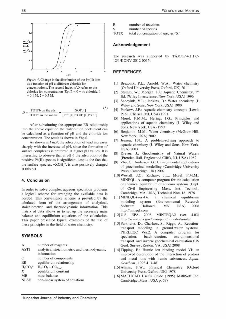
After substituting the appropriate ER relationship into the above equation the distribution coefficient can be calculated as a function of pH and the chloride ion concentration. The result is shown in Fig.4.

As shown in Fig.4, the adsorption of lead increases sharply with the increase of pH, since the formation of surface complexes is preferred at higher pH values. It is interesting to observe that at pH 6 the adsorption of the positive Pb(II) species is significant despite the fact that the surface species, ≡XOH2

+, is also positively charged at this pH.

4. Conclusion

In order to solve complex aqueous speciation problems a logical scheme for arranging the available data is needed. This convenience scheme is provided by the tabulated form of the arrangement of analytical, stoichiometric, and thermodynamic information. This matrix of data allows us to set up the necessary mass balance and equilibrium equations of the calculation. This paper presented typical examples of the use of these principles in the field of water chemistry.

SYMBOLS

A number of reagents ASTI analytical stoichiometric and thermodynamic

information C number of components ER equilibrium relationship H2CO3* H2CO3 + CO2(aq) K equilibrium constant MB mass balance NLSE non-linear system of equations

R number of reactions S number of species TOTX total concentration of species ‘X’

Acknowledgement

The research was supported by TÁMOP-4.1.1.C-12/1/KONV-2012-0015.

REFERENCES

[1] Brezonik, P.L.; Arnold, W.A.: Water chemistry (Oxford University Press, Oxford, UK) 2011

[2] Stumm, W.; Morgan, J.J.: Aquatic Chemistry, 3rd Ed. (Wiley Interscience, New York, USA) 1996

[3] Snoeyink, V.L.; Jenkins, D.: Water chemistry (J. Wiley and Sons, New York, USA) 1980

[4] Pankow, J.F.: Aquatic chemistry concepts (Lewis Publ., Chelsea, MI, USA) 1991

[5] Morel, F.M.M.; Hering, J.G.: Principles and applications of aquatic chemistry (J. Wiley and Sons, New York, USA) 1993

[6] Benjamin, M.M.: Water chemistry (McGraw-Hill, New York, USA) 2002

[7] Jensen, J.N.: A problem-solving approach to aquatic chemistry (J. Wiley and Sons, New York, USA) 2003

[8] Drever, J.: Geochemistry of Natural Waters (Prentice-Hall, Englewood Cliffs, NJ, USA) 1982

[9] Zhu, C.; Anderson, G.: Environmental applications of geochemical modelling (Cambridge University Press, Cambridge, UK) 2002

[10] Westall, J.C.; Zachary, J.L.; Morel, F.M.M.: MINEQL, A computer program for the calculation of chemical equilibrium of aqueous systems (Dept. of Civil Engineering, Mass. Inst. Technol., Cambridge, MA, USA) Technical Note 18, 1976

[11] MINEQL+ver.4.6, a chemical equilibrium modeling system (Environmental Research Software, Hallowell, MN, USA) 2008 http://mineql.com

[12] U.S. EPA. 2006. MINTEQA2 (ver. 4.03) http://www.epa.gov/ceampubl/mmedia/minteq

[13] Parkhurst, D.; Charlton, S.; Riggs, A.: Reaction-transport modeling in ground-water systems. PHREEQC Ver.2. A computer program for speciation, batch-reaction, one-dimensional transport, and inverse geochemical calculation (US Geol. Survey, Reston, VA, USA) 2008

[14] Tipping, E.: Humic ion binding model VI: an improved description of the interaction of protons and metal ions with humic substances. Aquat. Geochem., 1998 4, 3-48

[15] Atkins, P.W.: Physical Chemistry (Oxford University Press, Oxford, UK) 1978

[16] MATHCAD User’s Guide (1995) MathSoft Inc. Cambridge, Mass., USA p. 637

Figure 4. Change in the distribution of the Pb(II) ions as a function of pH at different chloride ion concentrations. The second index of D refers to the chloride ion concentration (Eq.(5)): 0 = no chloride, 1 = 0.1 M, 2 = 0.5 M.