Embed Size (px)
Citation preview

Ordinary Differential Equations with
Applications
Carmen Chicone
Springer

To Jenny, for giving me the gift of time.
Preface
This book is based on a two-semester course in ordinary differential equa-tions that I have taught to graduate students for two decades at the Uni-versity of Missouri. The scope of the narrative evolved over time froman embryonic collection of supplementary notes, through many classroomtested revisions, to a treatment of the subject that is suitable for a year (ormore) of graduate study.
If it is true that students of differential equations give away their point ofview by the way they denote the derivative with respect to the independentvariable, then the initiated reader can turn to Chapter 1, note that I writex, not x′, and thus correctly deduce that this book is written with an eyetoward dynamical systems. Indeed, this book contains a thorough intro-duction to the basic properties of differential equations that are needed toapproach the modern theory of (nonlinear) dynamical systems. However,this is not the whole story. The book is also a product of my desire todemonstrate to my students that differential equations is the least insularof mathematical subjects, that it is strongly connected to almost all areasof mathematics, and it is an essential element of applied mathematics.
When I teach this course, I use the first part of the first semester to pro-vide a rapid, student-friendly survey of the standard topics encountered inan introductory course of ordinary differential equations (ODE): existencetheory, flows, invariant manifolds, linearization, omega limit sets, phaseplane analysis, and stability. These topics, covered in Sections 1.1–1.8 ofChapter 1 of this book, are introduced, together with some of their im-portant and interesting applications, so that the power and beauty of thesubject is immediately apparent. This is followed by a discussion of linear
viii Preface
systems theory and the proofs of the basic theorems on linearized stabil-ity in Chapter 2. Then, I conclude the first semester by presenting oneor two realistic applications from Chapter 3. These applications provide acapstone for the course as well as an excellent opportunity to teach themathematics graduate students some physics, while giving the engineeringand physics students some exposure to applications from a mathematicalperspective.
In the second semester, I introduce some advanced concepts related toexistence theory, invariant manifolds, continuation of periodic orbits, forcedoscillators, separatrix splitting, averaging, and bifurcation theory. However,since there is not enough time in one semester to cover all of this materialin depth, I usually choose just one or two of these topics for presentation inclass. The material in the remaining chapters is assigned for private studyaccording to the interests of my students.
My course is designed to be accessible to students who have only stud-ied differential equations during one undergraduate semester. While I doassume some knowledge of linear algebra, advanced calculus, and analysis,only the most basic material from these subjects is required: eigenvalues andeigenvectors, compact sets, uniform convergence, the derivative of a func-tion of several variables, and the definition of metric and Banach spaces.With regard to the last prerequisite, I find that some students are afraidto take the course because they are not comfortable with Banach spacetheory. However, I put them at ease by mentioning that no deep propertiesof infinite dimensional spaces are used, only the basic definitions.
Exercises are an integral part of this book. As such, many of them areplaced strategically within the text, rather than at the end of a section.These interruptions of the flow of the narrative are meant to provide anopportunity for the reader to absorb the preceding material and as a guideto further study. Some of the exercises are routine, while others are sectionsof the text written in “exercise form.” For example, there are extended ex-ercises on structural stability, Hamiltonian and gradient systems on man-ifolds, singular perturbations, and Lie groups. My students are stronglyencouraged to work through the exercises. How is it possible to gain an un-derstanding of a mathematical subject without doing some mathematics?Perhaps a mathematics book is like a musical score: by sight reading youcan pick out the notes, but practice is required to hear the melody.
The placement of exercises is just one indication that this book is notwritten in axiomatic style. Many results are used before their proofs are pro-vided, some ideas are discussed without formal proofs, and some advancedtopics are introduced without being fully developed. The pure axiomaticapproach forbids the use of such devices in favor of logical order. The otherextreme would be a treatment that is intended to convey the ideas of thesubject with no attempt to provide detailed proofs of basic results. Whilethe narrative of an axiomatic approach can be as dry as dust, the excite-ment of an idea-oriented approach must be weighed against the fact that
Preface ix
it might leave most beginning students unable to grasp the subtlety of thearguments required to justify the mathematics. I have tried to steer a mid-dle course in which careful formulations and complete proofs are given forthe basic theorems, while the ideas of the subject are discussed in depthand the path from the pure mathematics to the physical universe is clearlymarked. I am reminded of an esteemed colleague who mentioned that acertain textbook “has lots of fruit, but no juice.” Above all, I have tried toavoid this criticism.
Application of the implicit function theorem is a recurring theme in thebook. For example, the implicit function theorem is used to prove the rec-tification theorem and the fundamental existence and uniqueness theoremsfor solutions of differential equations in Banach spaces. Also, the basic re-sults of perturbation and bifurcation theory, including the continuation ofsubharmonics, the existence of periodic solutions via the averaging method,as well as the saddle node and Hopf bifurcations, are presented as appli-cations of the implicit function theorem. Because of its central role, theimplicit function theorem and the terrain surrounding this important re-sult are discussed in detail. In particular, I present a review of calculus ina Banach space setting and use this theory to prove the contraction map-ping theorem, the uniform contraction mapping theorem, and the implicitfunction theorem.
This book contains some material that is not encountered in most treat-ments of the subject. In particular, there are several sections with the title“Origins of ODE,” where I give my answer to the question “What is thisgood for?” by providing an explanation for the appearance of differentialequations in mathematics and the physical sciences. For example, I showhow ordinary differential equations arise in classical physics from the fun-damental laws of motion and force. This discussion includes a derivationof the Euler–Lagrange equation, some exercises in electrodynamics, andan extended treatment of the perturbed Kepler problem. Also, I have in-cluded some discussion of the origins of ordinary differential equations inthe theory of partial differential equations. For instance, I explain the ideathat a parabolic partial differential equation can be viewed as an ordinarydifferential equation in an infinite dimensional space. In addition, travelingwave solutions and the Galerkin approximation technique are discussed.In a later “origins” section, the basic models for fluid dynamics are intro-duced. I show how ordinary differential equations arise in boundary layertheory. Also, the ABC flows are defined as an idealized fluid model, and Idemonstrate that this model has chaotic regimes. There is also a section oncoupled oscillators, a section on the Fermi–Ulam–Pasta experiments, andone on the stability of the inverted pendulum where a proof of linearizedstability under rapid oscillation is obtained using Floquet’s method andsome ideas from bifurcation theory. Finally, in conjunction with a treat-ment of the multiple Hopf bifurcation for planar systems, I present a short
x Preface
introduction to an algorithm for the computation of the Lyapunov quanti-ties as an illustration of computer algebra methods in bifurcation theory.
Another special feature of the book is an introduction to the fiber con-traction principle as a powerful tool for proving the smoothness of functionsthat are obtained as fixed points of contractions. This basic method is usedfirst in a proof of the smoothness of the flow of a differential equationwhere its application is transparent. Later, the fiber contraction principleappears in the nontrivial proof of the smoothness of invariant manifoldsat a rest point. In this regard, the proof for the existence and smoothnessof stable and center manifolds at a rest point is obtained as a corollary ofa more general existence theorem for invariant manifolds in the presenceof a “spectral gap.” These proofs can be extended to infinite dimensions.In particular, the applications of the fiber contraction principle and theLyapunov–Perron method in this book provide an introduction to some ofthe basic tools of invariant manifold theory.
The theory of averaging is treated from a fresh perspective that is in-tended to introduce the modern approach to this classical subject. A com-plete proof of the averaging theorem is presented, but the main theme ofthe chapter is partial averaging at a resonance. In particular, the “pen-dulum with torque” is shown to be a universal model for the motion of anonlinear oscillator near a resonance. This approach to the subject leadsnaturally to the phenomenon of “capture into resonance,” and it also pro-vides the necessary background for students who wish to read the literatureon multifrequency averaging, Hamiltonian chaos, and Arnold diffusion.
I prove the basic results of one-parameter bifurcation theory—the saddlenode and Hopf bifurcations—using the Lyapunov–Schmidt reduction. Thefact that degeneracies in a family of differential equations might be un-avoidable is explained together with a brief introduction to transversalitytheory and jet spaces. Also, the multiple Hopf bifurcation for planar vectorfields is discussed. In particular, and the Lyapunov quantities for polyno-mial vector fields at a weak focus are defined and this subject matter isused to provide a link to some of the algebraic techniques that appear innormal form theory.
Since almost all of the topics in this book are covered elsewhere, there isno claim of originality on my part. I have merely organized the material ina manner that I believe to be most beneficial to my students. By readingthis book, I hope that you will appreciate and be well prepared to use thewonderful subject of differential equations.
Columbia, Missouri Carmen ChiconeJune 1999
Acknowledgments
I would like to thank all the people who have offered valuable suggestionsfor corrections and additions to this book, especially, Sergei Kosakovsky,M. B. H. Rhouma, and Douglas Shafer. Also, I thank Dixie Fingerson formuch valuable assistance in the mathematics library.
Invitation
Please send your corrections or comments.E-mail: [email protected]: Department of Mathematics
University of MissouriColumbia, MO 65211
Contents
Preface vii
1 Introduction to Ordinary Differential Equations 11.1 Existence and Uniqueness . . . . . . . . . . . . . . . . . . . 11.2 Types of Differential Equations . . . . . . . . . . . . . . . . 41.3 Geometric Interpretation of Autonomous Systems . . . . . . 61.4 Flows . . . . . . . . . . . . . . . . . . . . . . . . . . . . . . 12
1.4.1 Reparametrization of Time . . . . . . . . . . . . . . 141.5 Stability and Linearization . . . . . . . . . . . . . . . . . . . 171.6 Stability and the Direct Method of Lyapunov . . . . . . . . 231.7 Introduction to Invariant Manifolds . . . . . . . . . . . . . . 28
1.7.1 Smooth Manifolds . . . . . . . . . . . . . . . . . . . 361.7.2 Tangent Spaces . . . . . . . . . . . . . . . . . . . . . 441.7.3 Change of Coordinates . . . . . . . . . . . . . . . . . 521.7.4 Polar Coordinates . . . . . . . . . . . . . . . . . . . 56
1.8 Periodic Solutions . . . . . . . . . . . . . . . . . . . . . . . 711.8.1 The Poincare Map . . . . . . . . . . . . . . . . . . . 711.8.2 Limit Sets and Poincare–Bendixson Theory . . . . . 79
1.9 Review of Calculus . . . . . . . . . . . . . . . . . . . . . . . 931.9.1 The Mean Value Theorem . . . . . . . . . . . . . . . 981.9.2 Integration in Banach Spaces . . . . . . . . . . . . . 1001.9.3 The Contraction Principle . . . . . . . . . . . . . . . 1061.9.4 The Implicit Function Theorem . . . . . . . . . . . . 116
1.10 Existence, Uniqueness, and Extensibility . . . . . . . . . . . 117
xiv Contents
2 Linear Systems and Stability 1272.1 Homogeneous Linear Differential Equations . . . . . . . . . 128
2.1.1 Gronwall’s Inequality . . . . . . . . . . . . . . . . . 1282.1.2 Homogeneous Linear Systems: General Theory . . . 1302.1.3 Principle of Superposition . . . . . . . . . . . . . . . 1312.1.4 Linear Equations with Constant Coefficients . . . . . 135
2.2 Stability of Linear Systems . . . . . . . . . . . . . . . . . . 1512.3 Stability of Nonlinear Systems . . . . . . . . . . . . . . . . 1552.4 Floquet Theory . . . . . . . . . . . . . . . . . . . . . . . . . 162
2.4.1 Lyapunov Exponents . . . . . . . . . . . . . . . . . . 1762.4.2 Hill’s Equation . . . . . . . . . . . . . . . . . . . . . 1792.4.3 Periodic Orbits of Linear Systems . . . . . . . . . . 1832.4.4 Stability of Periodic Orbits . . . . . . . . . . . . . . 185
3 Applications 1993.1 Origins of ODE: The Euler–Lagrange Equation . . . . . . . 1993.2 Origins of ODE: Classical Physics . . . . . . . . . . . . . . . 203
3.2.1 Motion of a Charged Particle . . . . . . . . . . . . . 2053.2.2 Motion of a Binary System . . . . . . . . . . . . . . 2063.2.3 Disturbed Kepler Motion and Delaunay Elements . . 2153.2.4 Satellite Orbiting an Oblate Planet . . . . . . . . . . 2223.2.5 The Diamagnetic Kepler Problem . . . . . . . . . . 228
3.3 Coupled Pendula: Beats . . . . . . . . . . . . . . . . . . . . 2333.4 The Fermi–Ulam–Pasta Oscillator . . . . . . . . . . . . . . 2363.5 The Inverted Pendulum . . . . . . . . . . . . . . . . . . . . 2413.6 Origins of ODE: Partial Differential Equations . . . . . . . 247
3.6.1 Infinite Dimensional ODE . . . . . . . . . . . . . . . 2493.6.2 Galerkin Approximation . . . . . . . . . . . . . . . . 2613.6.3 Traveling Waves . . . . . . . . . . . . . . . . . . . . 2743.6.4 First Order PDE . . . . . . . . . . . . . . . . . . . . 278
4 Hyperbolic Theory 2834.1 Invariant Manifolds . . . . . . . . . . . . . . . . . . . . . . . 2834.2 Applications of Invariant Manifolds . . . . . . . . . . . . . . 3024.3 The Hartman–Grobman Theorem . . . . . . . . . . . . . . . 305
4.3.1 Diffeomorphisms . . . . . . . . . . . . . . . . . . . . 3054.3.2 Differential Equations . . . . . . . . . . . . . . . . . 311
5 Continuation of Periodic Solutions 3175.1 A Classic Example: van der Pol’s Oscillator . . . . . . . . . 318
5.1.1 Continuation Theory and Applied Mathematics . . . 3245.2 Autonomous Perturbations . . . . . . . . . . . . . . . . . . 3265.3 Nonautonomous Perturbations . . . . . . . . . . . . . . . . 340
5.3.1 Rest Points . . . . . . . . . . . . . . . . . . . . . . . 3435.3.2 Isochronous Period Annulus . . . . . . . . . . . . . . 343
Contents xv
5.3.3 The Forced van der Pol Oscillator . . . . . . . . . . 3475.3.4 Regular Period Annulus . . . . . . . . . . . . . . . . 3565.3.5 Limit Cycles–Entrainment–Resonance Zones . . . . 3675.3.6 Lindstedt Series and the Perihelion of Mercury . . . 3745.3.7 Entrainment Domains for van der Pol’s Oscillator . 382
5.4 Forced Oscillators . . . . . . . . . . . . . . . . . . . . . . . . 384
6 Homoclinic Orbits, Melnikov’s Method, and Chaos 3916.1 Autonomous Perturbations: Separatrix Splitting . . . . . . 3966.2 Periodic Perturbations: Transverse Homoclinic Points . . . 4066.3 Origins of ODE: Fluid Dynamics . . . . . . . . . . . . . . . 421
6.3.1 The Equations of Fluid Motion . . . . . . . . . . . . 4226.3.2 ABC Flows . . . . . . . . . . . . . . . . . . . . . . . 4316.3.3 Chaotic ABC Flows . . . . . . . . . . . . . . . . . . 434
7 Averaging 4517.1 The Averaging Principle . . . . . . . . . . . . . . . . . . . . 4517.2 Averaging at Resonance . . . . . . . . . . . . . . . . . . . . 4607.3 Action-Angle Variables . . . . . . . . . . . . . . . . . . . . . 477
8 Local Bifurcation 4838.1 One-Dimensional State Space . . . . . . . . . . . . . . . . . 484
8.1.1 The Saddle-Node Bifurcation . . . . . . . . . . . . . 4848.1.2 A Normal Form . . . . . . . . . . . . . . . . . . . . . 4868.1.3 Bifurcation in Applied Mathematics . . . . . . . . . 4878.1.4 Families, Transversality, and Jets . . . . . . . . . . . 489
8.2 Saddle-Node Bifurcation by Lyapunov–Schmidt Reduction . 4968.3 Poincare–Andronov–Hopf Bifurcation . . . . . . . . . . . . 502
8.3.1 Multiple Hopf Bifurcation . . . . . . . . . . . . . . . 513
References 531
Index 545
1Introduction to Ordinary DifferentialEquations
This chapter is about the most basic concepts of the theory of differentialequations. We will answer some fundamental questions: What is a differen-tial equation? Do differential equations always have solutions? Are solutionsof differential equations unique? However, the most important goal of thischapter is to introduce a geometric interpretation for the space of solutionsof a differential equation. Using this geometry, we will introduce some ofthe elements of the subject: rest points, periodic orbits, and invariant man-ifolds. Finally, we will review the calculus in a Banach space setting anduse it to prove the classic theorems on the existence, uniqueness, and ex-tensibility of solutions. References for this chapter include [8], [11], [49],[51], [78], [83], [95], [107], [141], [164], and [179].
1.1 Existence and Uniqueness
Let J ⊆ R, U ⊆ Rn, and Λ ⊆ R
k be open subsets, and suppose thatf : J × U × Λ → R
n is a smooth function. Here the term “smooth” meansthat the function f is continuously differentiable. An ordinary differentialequation (ODE) is an equation of the form
x = f(t, x, λ) (1.1)
where the dot denotes differentiation with respect to the independent vari-able t (usually a measure of time), the dependent variable x is a vector ofstate variables, and λ is a vector of parameters. As convenient terminology,
2 1. Introduction to Ordinary Differential Equations
especially when we are concerned with the components of a vector differ-ential equation, we will say that equation (1.1) is a system of differentialequations. Also, if we are interested in changes with respect to parameters,then the differential equation is called a family of differential equations.
Example 1.1. The forced van der Pol oscillator
x1 = x2,
x2 = b(1 − x21)x2 − ω2x1 + a cos Ωt
is a differential equation with J = R, x = (x1, x2) ∈ U = R2,
Λ = (a, b, ω,Ω) : (a, b) ∈ R2, ω > 0, Ω > 0,
and f : R × R2 × Λ → R
2 defined in components by
(t, x1, x2, a, b, ω, Ω) → (x2, b(1 − x21)x2 − ω2x1 + a cos Ωt).
If λ ∈ Λ is fixed, then a solution of the differential equation (1.1) is afunction φ : J0 → U given by t → φ(t), where J0 is an open subset of J ,such that
dφ
dt(t) = f(t, φ(t), λ) (1.2)
for all t ∈ J0.In this context, the words “trajectory,” “phase curve,” and “integral
curve” are also used to refer to solutions of the differential equation (1.1).However, it is useful to have a term that refers to the image of the solutionin R
n. Thus, we define the orbit of the solution φ to be the set φ(t) ∈ U :t ∈ J0.
When a differential equation is used to model the evolution of a statevariable for a physical process, a fundamental problem is to determine thefuture values of the state variable from its initial value. The mathematicalmodel is then given by a pair of equations
x = f(t, x, λ), x(t0) = x0
where the second equation is called an initial condition. If the differentialequation is defined as equation (1.1) and (t0, x0) ∈ J × U , then the pairof equations is called an initial value problem. Of course, a solution of thisinitial value problem is just a solution φ of the differential equation suchthat φ(t0) = x0.
If we view the differential equation (1.1) as a family of differential equa-tions depending on the parameter vector and perhaps also on the initialcondition, then we can consider corresponding families of solutions—if theyexist—by listing the variables under consideration as additional arguments.For example, we will write t → φ(t, t0, x0, λ) to specify the dependence of
1.1 Existence and Uniqueness 3
a solution on the initial condition x(t0) = x0 and on the parameter vectorλ.
The fundamental issues of the general theory of differential equationsare the existence, uniqueness, extensibility, and continuity with respect toparameters of solutions of initial value problems. Fortunately, all of theseissues are resolved by the following foundational results of the subject:Every initial value problem has a unique solution that is smooth with respectto initial conditions and parameters. Moreover, the solution of an initialvalue problem can be extended in time until it either reaches the domain ofdefinition of the differential equation or blows up to infinity.
The next three theorems are the formal statements of the foundationalresults of the subject of differential equations. They are, of course, usedextensively in all that follows.
Theorem 1.2 (Existence and Uniqueness). If J ⊆ R, U ⊆ Rn, and
Λ ⊆ Rk are open sets, f : J × U × Λ → R
n is a smooth function, and(t0, x0, λ0) ∈ J × U × Λ, then there exist open subsets J0 ⊆ J , U0 ⊆ U ,Λ0 ⊆ Λ with (t0, x0, λ0) ∈ J0 × U0 × Λ0 and a function φ : J0 × J0 ×U0 × Λ0 → R
n given by (t, s, x, λ) → φ(t, s, x, λ) such that for each point(t1, x1, λ1) ∈ J0 × U0 × Λ0, the function t → φ(t, t1, x1, λ1) is the uniquesolution defined on J0 of the initial value problem given by the differentialequation (1.1) and the initial condition x(t1) = x1.
Recall that if k = 1, 2, . . . ,∞, a function defined on an open set is calledCk if the function together with all of its partial derivatives up to andincluding those of order k are continuous on the open set. Similarly, a func-tion is called real analytic if it has a convergent power series representationwith a positive radius of convergence at each point of the open set.
Theorem 1.3 (Continuous Dependence). If, for the system (1.1), thehypotheses of Theorem 1.2 are satisfied, then the solution φ : J0 ×J0 ×U0 ×Λ0 → R
n of the differential equation (1.1) is a smooth function. Moreover,if f is Ck for some k = 1, 2, . . . ,∞ (respectively, f is real analytic), thenφ is also Ck (respectively, real analytic).
As a convenient notation, we will write |x| for the usual Euclidean normof x ∈ R
n. However, because all norms on Rn are equivalent, the results of
this section are valid for an arbitrary norm on Rn.
Theorem 1.4 (Extensibility). If, for the system (1.1), the hypotheses ofTheorem 1.2 hold, and if the maximal open interval of existence of the so-lution t → φ(t) (with the last three of its arguments suppressed) is given by(α, β) with ∞ ≤ α < β < ∞, then |φ(t)| approaches ∞ or φ(t) approachesa point on the boundary of U as t → β.
In case there is some finite T and limt→T |φ(t)| approaches ∞, we saythe solution blows up in finite time.
4 1. Introduction to Ordinary Differential Equations
The existence and uniqueness theorem is so fundamental in science thatit is sometimes called the “principle of determinism.” The idea is that ifwe know the initial conditions, then we can predict the future states of thesystem. The principle of determinism is of course validated by the proofof the existence and uniqueness theorem. However, the interpretation ofthis principle for physical systems is not as clear as it might seem. Theproblem is that solutions of differential equations can be very complicated.For example, the future state of the system might depend sensitively onthe initial state of the system. Thus, if we do not know the initial stateexactly, the final state may be very difficult (if not impossible) to predict.
The variables that we will specify as explicit arguments for the solutionφ of a differential equation depend on the context, as we have mentionedabove. However, very often we will write t → φ(t, x) to denote the solutionsuch that φ(0, x) = x. Similarly, when we wish to specify the parameter vec-tor, we will use t → φ(t, x, λ) to denote the solution such that φ(0, x, λ) = x.
Example 1.5. The solution of the differential equation x = x2, x ∈ R, isgiven by the elementary function
φ(t, x) =x
1 − xt.
For this example, J = R and U = R. Note that φ(0, x) = x. If x > 0, thenthe corresponding solution only exists on the interval J0 = (−∞, x−1).Also, we have that |φ(t, x)| → ∞ as t → x−1. This illustrates one of thepossibilities mentioned in the extensibility theorem, namely, blow up infinite time.
Exercise 1.6. Consider the differential equation x = −√x, x ∈ R. Find the
solution with dependence on the initial point, and discuss the extensibility ofsolutions.
1.2 Types of Differential Equations
Differential equations may be classified in several different ways. In thissection we note that the independent variable may be implicit or explicit,and that higher order derivatives may appear.
An autonomous differential equation is given by
x = f(x, λ), x ∈ Rn, λ ∈ R
k; (1.3)
that is, the function f does not depend explicitly on the independent vari-able. If the function f does depend explicitly on t, then the correspondingdifferential equation is called nonautonomous.
1.2 Types of Differential Equations 5
In physical applications, we often encounter equations containing second,third, or higher order derivatives with respect to the independent variable.These are called second order differential equations, third order differentialequations, and so on, where the the order of the equation refers to the orderof the highest order derivative with respect to the independent variable thatappears explicitly. In this hierarchy, a differential equation is called a firstorder differential equation.
Recall that Newton’s second law—the rate of change of the linear mo-mentum acting on a body is equal to the sum of the forces acting onthe body—involves the second derivative of the position of the body withrespect to time. Thus, in many physical applications the most commondifferential equations used as mathematical models are second order differ-ential equations. For example, the natural physical derivation of van derPol’s equation leads to a second order differential equation of the form
u + b(u2 − 1)u + ω2u = a cos Ωt. (1.4)
An essential fact is that every differential equation is equivalent to a firstorder system. To illustrate, let us consider the conversion of van der Pol’sequation to a first order system. For this, we simply define a new variablev := u so that we obtain the following system:
u = v,
v = −ω2u + b(1 − u2)v + a cos Ωt. (1.5)
Clearly, this system is equivalent to the second order equation in the sensethat every solution of the system determines a solution of the second or-der van der Pol equation, and every solution of the van der Pol equationdetermines a solution of this first order system.
Let us note that there are many possibilities for the construction ofequivalent first order systems—we are not required to define v := u. Forexample, if we define v = au where a is a nonzero constant, and follow thesame procedure used to obtain system (1.5), then we will obtain a familyof equivalent first order systems. Of course, a differential equation of orderm can be converted to an equivalent first order system by defining m − 1new variables in the obvious manner.
If our model differential equation is a nonautonomous differential equa-tion of the form x = f(t, x), where we have suppressed the possible de-pendence on parameters, then there is an “equivalent” autonomous systemobtained by defining a new variable as follows:
x = f(τ, x),τ = 1. (1.6)
For example, if t → (φ(t), τ(t)) is a solution of this system with φ(t0) = x0and τ(t0) = t0, then τ(t) = t and
φ(t) = f(t, φ(t)), φ(t0) = x0.
6 1. Introduction to Ordinary Differential Equations
Thus, the function t → φ(t) is a solution of the initial value problem
x = f(t, x), x(t0) = x0.
In particular, every solution of the nonautonomous differential equationcan be obtained from a solution of the autonomous system (1.6).
We have just seen that all ordinary differential equations correspond tofirst order autonomous systems. As a result, we will pay special attentionto the properties of autonomous systems. In most cases, the conversion ofa higher order differential equation to a first order system is useful. Onthe other hand, the conversion of nonautonomous equations (or systems)to autonomous systems is not always wise. However, there is one notableexception. Indeed, if a nonautonomous system is given by x = f(t, x) wheref is a periodic function of t, then, as we will see, the conversion to anautonomous system is very often the best way to analyze the system.
Exercise 1.7. Find a first order system that is equivalent to the third orderdifferential equation
εx′′′ + xx′′ − (x′)2 + 1 = 0
where ε is a parameter and the ′ denotes differentiation with respect to theindependent variable.
1.3 Geometric Interpretation of AutonomousSystems
In this section we will describe a very important geometric interpretationof the autonomous differential equation
x = f(x), x ∈ Rn. (1.7)
The function given by x → (x, f(x)) defines a vector field on Rn associ-
ated with the differential equation (1.7). Here the first component of thefunction specifies the base point and the second component specifies thevector at this base point. A solution t → φ(t) of (1.7) has the property thatits tangent vector at each time t is given by
(φ(t), φ(t)) = (φ(t), f(φ(t))).
In other words, if ξ ∈ Rn is on the orbit of this solution, then the tangent
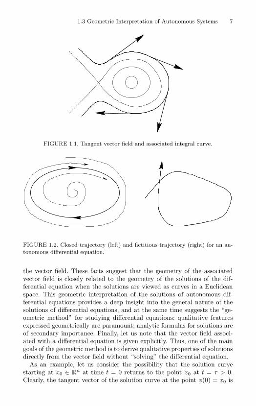
line to the orbit at ξ is generated by the vector (ξ, f(ξ)), as depicted inFigure 1.1.
We have just mentioned two essential facts: (i) There is a one-to-onecorrespondence between vector fields and autonomous differential equa-tions. (ii) Every tangent vector to a solution curve is given by a vector in
1.3 Geometric Interpretation of Autonomous Systems 7
FIGURE 1.1. Tangent vector field and associated integral curve.
FIGURE 1.2. Closed trajectory (left) and fictitious trajectory (right) for an au-tonomous differential equation.
the vector field. These facts suggest that the geometry of the associatedvector field is closely related to the geometry of the solutions of the dif-ferential equation when the solutions are viewed as curves in a Euclideanspace. This geometric interpretation of the solutions of autonomous dif-ferential equations provides a deep insight into the general nature of thesolutions of differential equations, and at the same time suggests the “ge-ometric method” for studying differential equations: qualitative featuresexpressed geometrically are paramount; analytic formulas for solutions areof secondary importance. Finally, let us note that the vector field associ-ated with a differential equation is given explicitly. Thus, one of the maingoals of the geometric method is to derive qualitative properties of solutionsdirectly from the vector field without “solving” the differential equation.
As an example, let us consider the possibility that the solution curvestarting at x0 ∈ R
n at time t = 0 returns to the point x0 at t = τ > 0.Clearly, the tangent vector of the solution curve at the point φ(0) = x0 is
8 1. Introduction to Ordinary Differential Equations
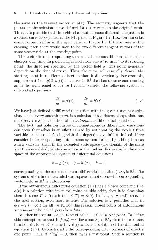
the same as the tangent vector at φ(τ). The geometry suggests that thepoints on the solution curve defined for t > τ retraces the original orbit.Thus, it is possible that the orbit of an autonomous differential equation isa closed curve as depicted in the left panel of Figure 1.2. However, an orbitcannot cross itself as in the right panel of Figure 1.2. If there were such acrossing, then there would have to be two different tangent vectors of thesame vector field at the crossing point.
The vector field corresponding to a nonautonomous differential equationchanges with time. In particular, if a solution curve “returns” to its startingpoint, the direction specified by the vector field at this point generallydepends on the time of arrival. Thus, the curve will generally “leave” thestarting point in a different direction than it did originally. For example,suppose that t → (g(t), h(t)) is a curve in R
2 that has a transverse crossingas in the right panel of Figure 1.2, and consider the following system ofdifferential equations
dx
dt= g′(t),
dy
dt= h′(t). (1.8)
We have just defined a differential equation with the given curve as a solu-tion. Thus, every smooth curve is a solution of a differential equation, butnot every curve is a solution of an autonomous differential equation.
The fact that solution curves of nonautonomous differential equationscan cross themselves is an effect caused by not treating the explicit timevariable on an equal footing with the dependent variables. Indeed, if weconsider the corresponding autonomous system formed by adding time asa new variable, then, in the extended state space (the domain of the stateand time variables), orbits cannot cross themselves. For example, the statespace of the autonomous system of differential equations
x = g′(τ), y = h′(τ), τ = 1,
corresponding to the nonautonomous differential equation (1.8), is R3. The
system’s orbits in the extended state space cannot cross—the correspondingvector field in R
3 is autonomous.If the autonomous differential equation (1.7) has a closed orbit and t →
φ(t) is a solution with its initial value on this orbit, then it is clear thatthere is some T > 0 such that φ(T ) = φ(0). In fact, as we will show inthe next section, even more is true: The solution is T -periodic; that is,φ(t + T ) = φ(t) for all t ∈ R. For this reason, closed orbits of autonomoussystems are also called periodic orbits.
Another important special type of orbit is called a rest point. To definethis concept, note that if f(x0) = 0 for some x0 ∈ R
n, then the constantfunction φ : R → R
n defined by φ(t) ≡ x0 is a solution of the differentialequation (1.7). Geometrically, the corresponding orbit consists of exactlyone point. Thus, if f(x0) = 0, then x0 is a rest point. Such a solution is

1.3 Geometric Interpretation of Autonomous Systems 9
FIGURE 1.3. A curve in phase space consisting of four orbits of an autonomousdifferential equation.
also called a steady state, a critical point, an equilibrium point, or a zero(of the associated vector field).
What are all the possible orbit types for autonomous differential equa-tions? The answer depends on what we mean by “types.” However, we havealready given a partial answer: An orbit can be a point, a simple closedcurve, or the homeomorphic image of an interval. A geometric picture ofall the orbits of an autonomous differential equation is called its phase por-trait or phase diagram. This terminology comes from the notion of phasespace in physics, the space of positions and momenta. But here the phasespace is simply the space R
n, the domain of the vector field that definesthe autonomous differential equation. For the record, the state space inphysics is the space of positions and velocities. However, when used in thecontext of abstract vector fields, the terms state space and phase space aresynonymous. The fundamental problem of the geometric theory of differen-tial equations is evident: Given a differential equation, determine its phaseportrait.
Because there are essentially only the three types of orbits mentioned inthe last paragraph, it might seem that phase portraits would not be toocomplicated. However, as we will see, even the portrait of a single orbit canbe very complex. Indeed, the homeomorphic image of an interval can be avery complicated subset in a Euclidean space. As a simple but importantexample of a complex geometric feature of a phase portrait, let us note thecurve that crosses itself in Figure 1.1. Such a curve cannot be an orbit ofan autonomous differential equation. However, if the crossing point on thedepicted curve is a rest point of the differential equation, then such a curvecan exist in the phase portrait as a union of the four orbits indicated inFigure 1.3.
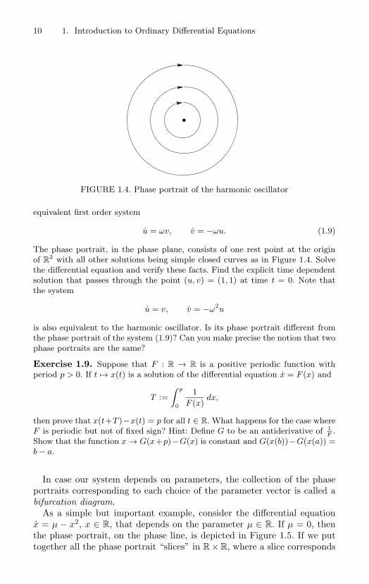
Exercise 1.8. Consider the harmonic oscillator (a model for an undampedspring) given by the second order differential equation u + ω2u = 0 with the
10 1. Introduction to Ordinary Differential Equations
FIGURE 1.4. Phase portrait of the harmonic oscillator
equivalent first order system
u = ωv, v = −ωu. (1.9)
The phase portrait, in the phase plane, consists of one rest point at the originof R
2 with all other solutions being simple closed curves as in Figure 1.4. Solvethe differential equation and verify these facts. Find the explicit time dependentsolution that passes through the point (u, v) = (1, 1) at time t = 0. Note thatthe system
u = v, v = −ω2u
is also equivalent to the harmonic oscillator. Is its phase portrait different fromthe phase portrait of the system (1.9)? Can you make precise the notion that twophase portraits are the same?
Exercise 1.9. Suppose that F : R → R is a positive periodic function withperiod p > 0. If t → x(t) is a solution of the differential equation x = F (x) and
T :=∫ p
0
1F (x)
dx,
then prove that x(t+T )−x(t) = p for all t ∈ R. What happens for the case whereF is periodic but not of fixed sign? Hint: Define G to be an antiderivative of 1
F.
Show that the function x → G(x+p)−G(x) is constant and G(x(b))−G(x(a)) =b − a.
In case our system depends on parameters, the collection of the phaseportraits corresponding to each choice of the parameter vector is called abifurcation diagram.
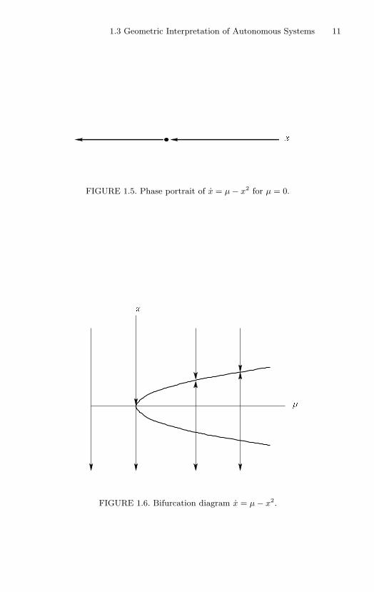
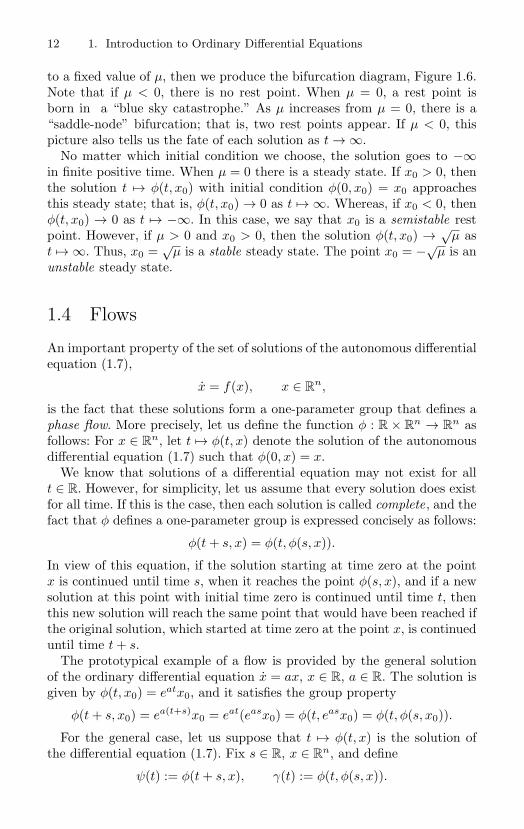
As a simple but important example, consider the differential equationx = µ − x2, x ∈ R, that depends on the parameter µ ∈ R. If µ = 0, thenthe phase portrait, on the phase line, is depicted in Figure 1.5. If we puttogether all the phase portrait “slices” in R × R, where a slice corresponds
1.3 Geometric Interpretation of Autonomous Systems 11
x
FIGURE 1.5. Phase portrait of x = µ − x2 for µ = 0.
x
FIGURE 1.6. Bifurcation diagram x = µ − x2.
12 1. Introduction to Ordinary Differential Equations
to a fixed value of µ, then we produce the bifurcation diagram, Figure 1.6.Note that if µ < 0, there is no rest point. When µ = 0, a rest point isborn in a “blue sky catastrophe.” As µ increases from µ = 0, there is a“saddle-node” bifurcation; that is, two rest points appear. If µ < 0, thispicture also tells us the fate of each solution as t → ∞.
No matter which initial condition we choose, the solution goes to −∞in finite positive time. When µ = 0 there is a steady state. If x0 > 0, thenthe solution t → φ(t, x0) with initial condition φ(0, x0) = x0 approachesthis steady state; that is, φ(t, x0) → 0 as t → ∞. Whereas, if x0 < 0, thenφ(t, x0) → 0 as t → −∞. In this case, we say that x0 is a semistable restpoint. However, if µ > 0 and x0 > 0, then the solution φ(t, x0) → √
µ ast → ∞. Thus, x0 =
√µ is a stable steady state. The point x0 = −√
µ is anunstable steady state.
1.4 Flows
An important property of the set of solutions of the autonomous differentialequation (1.7),
x = f(x), x ∈ Rn,
is the fact that these solutions form a one-parameter group that defines aphase flow. More precisely, let us define the function φ : R × R
n → Rn as
follows: For x ∈ Rn, let t → φ(t, x) denote the solution of the autonomous
differential equation (1.7) such that φ(0, x) = x.We know that solutions of a differential equation may not exist for all
t ∈ R. However, for simplicity, let us assume that every solution does existfor all time. If this is the case, then each solution is called complete, and thefact that φ defines a one-parameter group is expressed concisely as follows:
φ(t + s, x) = φ(t, φ(s, x)).
In view of this equation, if the solution starting at time zero at the pointx is continued until time s, when it reaches the point φ(s, x), and if a newsolution at this point with initial time zero is continued until time t, thenthis new solution will reach the same point that would have been reached ifthe original solution, which started at time zero at the point x, is continueduntil time t + s.
The prototypical example of a flow is provided by the general solutionof the ordinary differential equation x = ax, x ∈ R, a ∈ R. The solution isgiven by φ(t, x0) = eatx0, and it satisfies the group property
φ(t + s, x0) = ea(t+s)x0 = eat(easx0) = φ(t, easx0) = φ(t, φ(s, x0)).
For the general case, let us suppose that t → φ(t, x) is the solution ofthe differential equation (1.7). Fix s ∈ R, x ∈ R
n, and define
ψ(t) := φ(t + s, x), γ(t) := φ(t, φ(s, x)).
1.4 Flows 13
Note that φ(s, x) is a point in Rn. Therefore, γ is a solution of the differ-
ential equation (1.7) with γ(0) = φ(s, x). The function ψ is also a solutionof the differential equation because
dψ
dt=
dφ
dt(t + s, x) = f(φ(t + s, x)) = f(ψ(t)).
Finally, note that ψ(0) = φ(s, x) = γ(0). We have proved that both t →ψ(t) and t → γ(t) are solutions of the same initial value problem. Thus, bythe uniqueness theorem, γ(t) ≡ ψ(t). The idea of this proof—two functionsthat satisfy the same initial value problem are identical—is often used inthe theory and the applications of differential equations.
By the theorem on continuous dependence, φ is a smooth function. Inparticular, for each fixed t ∈ R, the function x → φ(t, x) is a smoothtransformation of R
n. In particular, if t = 0, then x → φ(0, x) is theidentity transformation. Let us also note that
x = φ(0, x) = φ(t − t, x) = φ(t, φ(−t, x)) = φ(−t, φ(t, x)).
In other words, x → φ(−t, x) is the inverse of the function x → φ(t, x).Thus, in fact, x → φ(t, x) is a diffeomorphism for each fixed t ∈ R.
If J × U is a product open subset of R × Rn, and if φ : J × U → R
n
is a function given by (t, x) → φ(t, x) such that φ(0, x) ≡ x and suchthat φ(t + s, x) = φ(t, φ(s, x)) whenever both sides of the equation aredefined, then we say that φ is a flow. Of course, if t → φ(t, x) defines thefamily of solutions of the autonomous differential equation (1.7) such thatφ(0, x) ≡ x, then φ is a flow.
Exercise 1.10. For each integer p, construct the flow of the differential equa-tion x = xp.
Exercise 1.11. Consider the differential equation x = t. Construct the familyof solutions t → φ(t, ξ) such that φ(0, ξ) = ξ for ξ ∈ R. Does φ define a flow?Explain.
Suppose that x0 ∈ Rn, T > 0, and that φ(T, x0) = x0; that is, the
solution returns to its initial point after time T . Then φ(t + T, x0) =φ(t, φ(T, x0)) = φ(t, x0). In other words, t → φ(t, x0) is a periodic func-tion with period T . The smallest number T > 0 with this property is calledthe period of the periodic orbit through x0.
Exercise 1.12. Write u + αu = 0, u ∈ R, α ∈ R as a first order system.Determine the flow of the system, and verify the flow property directly. Also,describe the bifurcation diagram of the system.
Exercise 1.13. Determine the flow of the first order system
x = y2 − x2, y = −2xy.
14 1. Introduction to Ordinary Differential Equations
Show that (almost) every orbit lies on an circle. Note that the flow gives rationalparameterizations for the circular orbits. Hint: Define z := x + iy.
In the mathematics literature, the notations t → φt(x) and t → φt(x)are often used in place of t → φ(t, x) for the solution of the differentialequation
x = f(x), x ∈ Rn,
that starts at x at time t = 0. We will use all three notations. The onlypossible confusion arises when subscripts are used for partial derivatives.However, the meaning of the notation will be clear from the context inwhich it appears.
1.4.1 Reparametrization of TimeSuppose that U is an open set in R
n, f : U → Rn is a smooth function, and
g : U → R is a positive smooth function. What is the relationship amongthe solutions of the differential equations
x = f(x), (1.10)x = g(x)f(x)? (1.11)
The vector fields defined by f and gf have the same direction at eachpoint in U , only their lengths are different. Thus, by our geometric inter-pretation of autonomous differential equations, it is intuitively clear thatthe differential equations (1.10) and (1.11) have the same phase portraitsin U . This fact is a corollary of the next proposition.
Proposition 1.14. If J ⊂ R is an open interval containing the origin andγ : J → R
n is a solution of the differential equation (1.10) with γ(0) =x0 ∈ U , then the function B : J → R given by
B(t) =∫ t
0
1g(γ(s))
ds
is invertible on its range K ⊆ R. If ρ : K → J is the inverse of B, thenthe identity
ρ′(t) = g(γ(ρ(t))
holds for all t ∈ K, and the function σ : K → Rn given by σ(t) = γ(ρ(t)) is
the solution of the differential equation (1.11) with initial condition σ(0) =x0.
1.4 Flows 15
Proof. The function s → 1/g(γ(s)) is continuous on J . So B is definedon J and its derivative is everywhere positive. Thus, B is invertible on itsrange. If ρ is its inverse, then
ρ′(t) =1
B′(ρ(t))= g(γ(ρ(t))),
and
σ′(t) = ρ′(t)γ′(ρ(t)) = g(γ(ρ(t))f(γ(ρ(t)) = g(σ(t))f(σ(t)).
Exercise 1.15. Use Proposition 1.14 to prove that differential equations (1.10)and (1.11) have the same phase portrait in U .
The fact that ρ in Proposition 1.14 is the inverse of B can be expressedby the formula
t =∫ ρ
0
1g(γ(s))
ds.
Thus, if we view ρ as a new time-like variable (that is, a variable thatincreases with time), then we have
dt
dρ=
1g(γ(ρ))
,
and therefore the differential equation (1.11), with the change of indepen-dent variable from t to ρ, is given by
dx
dρ=
dx
dt
dt
dρ= f(x).
In particular, this is just differential equation (1.10) with the independentvariable renamed.
The same result is obtained from a different point of view by using thedefinition of the solution of a differential equation to obtain the identity
d
dt[γ(ρ(t))] = g(γ(ρ(t)))f(γ(ρ(t))).
Equivalently, we have that
ρ′(t)γ′(ρ(t)) = g(γ(ρ(t)))f(γ(ρ(t))),
and therefore
γ′(ρ(t)) = f(γ(ρ(t))).
16 1. Introduction to Ordinary Differential Equations
If we view this equation as a differential equation for γ, then we can expressit in the form
dγ
dρ= f(γ(ρ)).
As a convenient expression, we say that the differential equation (1.10)is obtained from the differential equation (1.11) by a reparametrization oftime.
In the most important special cases the function g is constant. If its con-stant value is c > 0, then the reparametrization of the differential equationx = cf(x) by ρ = ct results in the new differential equation
dx
dρ= f(x).
Reparametrization in these cases is also called rescaling.Note that rescaling, as in the last paragraph, of the differential equation
x = cf(x) produces a differential equation in which the parameter c hasbeen eliminated. This idea is often used to simplify differential equations.Also, the same rescaling is used in applied mathematics to render the inde-pendent variable dimensionless. For example, if the original time variable tis measured in seconds, and the scale factor c has the units of 1/sec, thenthe new variable ρ is dimensionless.
The next proposition is a special case of the following claim: Every au-tonomous differential equation has a complete reparametrization (see Ex-ercise 1.19).
Proposition 1.16. If the differential equation x = f(x) is defined on Rn,
then the differential equation
x =1
1 + |f(x)|2 f(x) (1.12)
is defined on Rn and its flow is complete.
Proof. The vector field corresponding to the differential equation (1.12) issmoothly defined on all of R
n. If σ is one of its solutions with initial valueσ(0) = x0 and t is in the domain of σ, then, by integration with respect tothe independent variable, we have that
σ(t) − σ(0) =∫ t
0
11 + |f(σ(s))|2 f(σ(s)) ds.
Note that the integrand has norm less than one and use the triangle in-equality (taking into account the fact that t might be negative) to obtainthe following estimate:
|σ(t)| ≤ |x0| + |t|.
1.5 Stability and Linearization 17
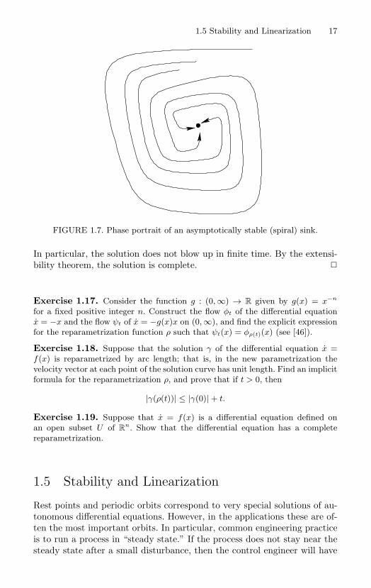
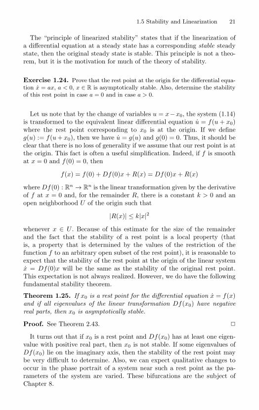
FIGURE 1.7. Phase portrait of an asymptotically stable (spiral) sink.
In particular, the solution does not blow up in finite time. By the extensi-bility theorem, the solution is complete.
Exercise 1.17. Consider the function g : (0, ∞) → R given by g(x) = x−n
for a fixed positive integer n. Construct the flow φt of the differential equationx = −x and the flow ψt of x = −g(x)x on (0, ∞), and find the explicit expressionfor the reparametrization function ρ such that ψt(x) = φρ(t)(x) (see [46]).
Exercise 1.18. Suppose that the solution γ of the differential equation x =f(x) is reparametrized by arc length; that is, in the new parametrization thevelocity vector at each point of the solution curve has unit length. Find an implicitformula for the reparametrization ρ, and prove that if t > 0, then
|γ(ρ(t))| ≤ |γ(0)| + t.
Exercise 1.19. Suppose that x = f(x) is a differential equation defined onan open subset U of R
n. Show that the differential equation has a completereparametrization.
1.5 Stability and Linearization
Rest points and periodic orbits correspond to very special solutions of au-tonomous differential equations. However, in the applications these are of-ten the most important orbits. In particular, common engineering practiceis to run a process in “steady state.” If the process does not stay near thesteady state after a small disturbance, then the control engineer will have
18 1. Introduction to Ordinary Differential Equations
U
x
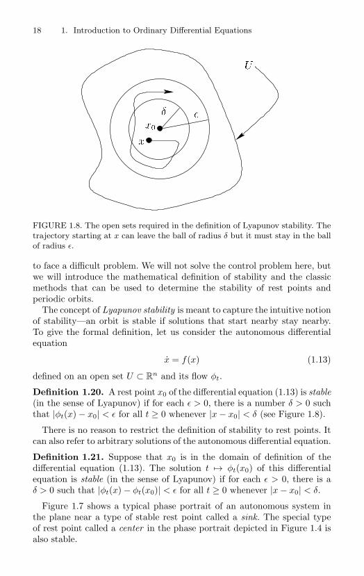
x
FIGURE 1.8. The open sets required in the definition of Lyapunov stability. Thetrajectory starting at x can leave the ball of radius δ but it must stay in the ballof radius ε.
to face a difficult problem. We will not solve the control problem here, butwe will introduce the mathematical definition of stability and the classicmethods that can be used to determine the stability of rest points andperiodic orbits.
The concept of Lyapunov stability is meant to capture the intuitive notionof stability—an orbit is stable if solutions that start nearby stay nearby.To give the formal definition, let us consider the autonomous differentialequation
x = f(x) (1.13)
defined on an open set U ⊂ Rn and its flow φt.
Definition 1.20. A rest point x0 of the differential equation (1.13) is stable(in the sense of Lyapunov) if for each ε > 0, there is a number δ > 0 suchthat |φt(x) − x0| < ε for all t ≥ 0 whenever |x − x0| < δ (see Figure 1.8).
There is no reason to restrict the definition of stability to rest points. Itcan also refer to arbitrary solutions of the autonomous differential equation.
Definition 1.21. Suppose that x0 is in the domain of definition of thedifferential equation (1.13). The solution t → φt(x0) of this differentialequation is stable (in the sense of Lyapunov) if for each ε > 0, there is aδ > 0 such that |φt(x) − φt(x0)| < ε for all t ≥ 0 whenever |x − x0| < δ.
Figure 1.7 shows a typical phase portrait of an autonomous system inthe plane near a type of stable rest point called a sink. The special typeof rest point called a center in the phase portrait depicted in Figure 1.4 isalso stable.
1.5 Stability and Linearization 19
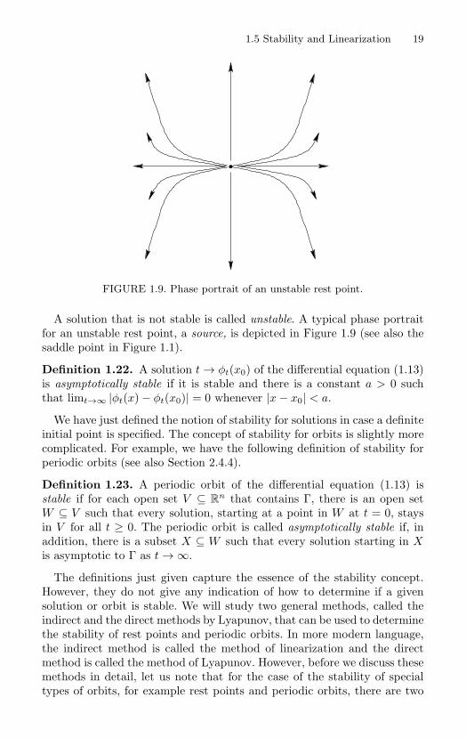
FIGURE 1.9. Phase portrait of an unstable rest point.
A solution that is not stable is called unstable. A typical phase portraitfor an unstable rest point, a source, is depicted in Figure 1.9 (see also thesaddle point in Figure 1.1).
Definition 1.22. A solution t → φt(x0) of the differential equation (1.13)is asymptotically stable if it is stable and there is a constant a > 0 suchthat limt→∞ |φt(x) − φt(x0)| = 0 whenever |x − x0| < a.
We have just defined the notion of stability for solutions in case a definiteinitial point is specified. The concept of stability for orbits is slightly morecomplicated. For example, we have the following definition of stability forperiodic orbits (see also Section 2.4.4).
Definition 1.23. A periodic orbit of the differential equation (1.13) isstable if for each open set V ⊆ R
n that contains Γ, there is an open setW ⊆ V such that every solution, starting at a point in W at t = 0, staysin V for all t ≥ 0. The periodic orbit is called asymptotically stable if, inaddition, there is a subset X ⊆ W such that every solution starting in Xis asymptotic to Γ as t → ∞.
The definitions just given capture the essence of the stability concept.However, they do not give any indication of how to determine if a givensolution or orbit is stable. We will study two general methods, called theindirect and the direct methods by Lyapunov, that can be used to determinethe stability of rest points and periodic orbits. In more modern language,the indirect method is called the method of linearization and the directmethod is called the method of Lyapunov. However, before we discuss thesemethods in detail, let us note that for the case of the stability of specialtypes of orbits, for example rest points and periodic orbits, there are two
20 1. Introduction to Ordinary Differential Equations
main problems: (i) Locating the special solutions. (ii) Determining theirstability.
For the remainder of this section and the next, the discussion will be re-stricted to the analysis for rest points. Our introduction to the methods forlocating and determining the stability of periodic orbits must be postponeduntil some additional concepts have been introduced.
Let us note that the problem of the location of rest points for the dif-ferential equation x = f(x) is exactly the problem of finding the roots ofthe equation f(x) = 0. Of course, finding roots may be a formidable task,especially if the function f depends on parameters and we wish to findits bifurcation diagram. In fact, in the search for rest points, sophisticatedtechniques of algebra, analysis, and numerical analysis are often required.This is not surprising when we stop to think that solving equations is oneof the fundamental themes in mathematics. For example, it is probably nottoo strong to say that the most basic problem in linear algebra, abstractalgebra, and algebraic geometry is the solution of systems of polynomialequations. The results of all of these subjects are sometimes needed to solveproblems in differential equations.
Let us suppose that we have identified some point x0 ∈ Rn such that
f(x0) = 0. What can we say about the stability of the corresponding restpoint? One of the great ideas in the subject of differential equations—not tomention other areas of mathematics—is linearization. This idea, in perhapsits purest form, is used to obtain the premier method for the determina-tion of the stability of rest points. The linearization method is based ontwo facts: (i) Stability analysis for linear systems is “easy.” (ii) Nonlinearsystems can be approximated by linear systems. These facts are just reflec-tions of the fundamental idea of differential calculus: Replace a nonlinearfunction by its derivative!
To describe the linearization method for rest points, let us consider (ho-mogeneous) linear systems of differential equations; that is, systems of theform x = Ax where x ∈ R
n and A is a linear transformation of Rn. If the
matrix A does not depend on t—so that the linear system is autonomous—then there is an effective method that can be used to determine the stabilityof its rest point at x = 0. In fact, we will show in Chapter 2 that if all ofthe eigenvalues of A have negative real parts, then x = 0 is an asymptot-ically stable rest point for the linear system. (The eigenvalues of a lineartransformation are defined on page 135.)
If x0 is a rest point for the nonlinear system x = f(x), then there is anatural way to produce a linear system that approximates the nonlinearsystem near x0: Simply replace the function f in the differential equationwith the linear function x → Df(x0)(x − x0) given by the first nonzeroterm of the Taylor series of f at x0. The linear differential equation
x = Df(x0)(x − x0) (1.14)
is called the linearized system associated with x = f(x) at x0.
1.5 Stability and Linearization 21
The “principle of linearized stability” states that if the linearization ofa differential equation at a steady state has a corresponding stable steadystate, then the original steady state is stable. This principle is not a theo-rem, but it is the motivation for much of the theory of stability.
Exercise 1.24. Prove that the rest point at the origin for the differential equa-tion x = ax, a < 0, x ∈ R is asymptotically stable. Also, determine the stabilityof this rest point in case a = 0 and in case a > 0.
Let us note that by the change of variables u = x−x0, the system (1.14)is transformed to the equivalent linear differential equation u = f(u + x0)where the rest point corresponding to x0 is at the origin. If we defineg(u) := f(u + x0), then we have u = g(u) and g(0) = 0. Thus, it should beclear that there is no loss of generality if we assume that our rest point is atthe origin. This fact is often a useful simplification. Indeed, if f is smoothat x = 0 and f(0) = 0, then
f(x) = f(0) + Df(0)x + R(x) = Df(0)x + R(x)
where Df(0) : Rn → R
n is the linear transformation given by the derivativeof f at x = 0 and, for the remainder R, there is a constant k > 0 and anopen neighborhood U of the origin such that
|R(x)| ≤ k|x|2
whenever x ∈ U . Because of this estimate for the size of the remainderand the fact that the stability of a rest point is a local property (thatis, a property that is determined by the values of the restriction of thefunction f to an arbitrary open subset of the rest point), it is reasonable toexpect that the stability of the rest point at the origin of the linear systemx = Df(0)x will be the same as the stability of the original rest point.This expectation is not always realized. However, we do have the followingfundamental stability theorem.
Theorem 1.25. If x0 is a rest point for the differential equation x = f(x)and if all eigenvalues of the linear transformation Df(x0) have negativereal parts, then x0 is asymptotically stable.
Proof. See Theorem 2.43.
It turns out that if x0 is a rest point and Df(x0) has at least one eigen-value with positive real part, then x0 is not stable. If some eigenvalues ofDf(x0) lie on the imaginary axis, then the stability of the rest point maybe very difficult to determine. Also, we can expect qualitative changes tooccur in the phase portrait of a system near such a rest point as the pa-rameters of the system are varied. These bifurcations are the subject ofChapter 8.
22 1. Introduction to Ordinary Differential Equations
Exercise 1.26. Prove: If x = 0, x ∈ R, then x = 0 is Lyapunov stable. Considerthe differential equations x = x3 and x = −x3. Prove that whereas the originis not a Lyapunov stable rest point for the differential equation x = x3, it isLyapunov stable for the differential equation x = −x3. Note that the linearizeddifferential equation at x = 0 in both cases is the same; namely, x = 0.
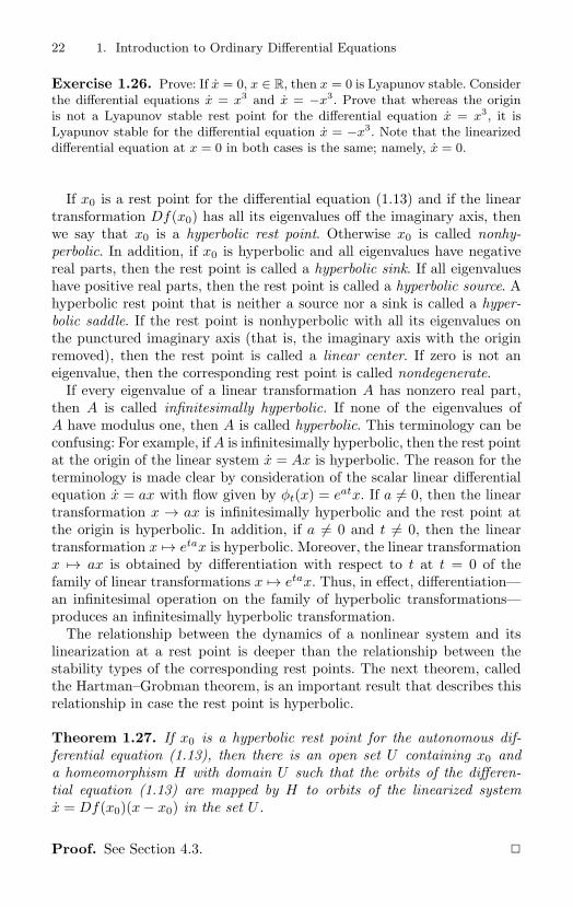
If x0 is a rest point for the differential equation (1.13) and if the lineartransformation Df(x0) has all its eigenvalues off the imaginary axis, thenwe say that x0 is a hyperbolic rest point. Otherwise x0 is called nonhy-perbolic. In addition, if x0 is hyperbolic and all eigenvalues have negativereal parts, then the rest point is called a hyperbolic sink. If all eigenvalueshave positive real parts, then the rest point is called a hyperbolic source. Ahyperbolic rest point that is neither a source nor a sink is called a hyper-bolic saddle. If the rest point is nonhyperbolic with all its eigenvalues onthe punctured imaginary axis (that is, the imaginary axis with the originremoved), then the rest point is called a linear center. If zero is not aneigenvalue, then the corresponding rest point is called nondegenerate.
If every eigenvalue of a linear transformation A has nonzero real part,then A is called infinitesimally hyperbolic. If none of the eigenvalues ofA have modulus one, then A is called hyperbolic. This terminology can beconfusing: For example, if A is infinitesimally hyperbolic, then the rest pointat the origin of the linear system x = Ax is hyperbolic. The reason for theterminology is made clear by consideration of the scalar linear differentialequation x = ax with flow given by φt(x) = eatx. If a = 0, then the lineartransformation x → ax is infinitesimally hyperbolic and the rest point atthe origin is hyperbolic. In addition, if a = 0 and t = 0, then the lineartransformation x → etax is hyperbolic. Moreover, the linear transformationx → ax is obtained by differentiation with respect to t at t = 0 of thefamily of linear transformations x → etax. Thus, in effect, differentiation—an infinitesimal operation on the family of hyperbolic transformations—produces an infinitesimally hyperbolic transformation.
The relationship between the dynamics of a nonlinear system and itslinearization at a rest point is deeper than the relationship between thestability types of the corresponding rest points. The next theorem, calledthe Hartman–Grobman theorem, is an important result that describes thisrelationship in case the rest point is hyperbolic.
Theorem 1.27. If x0 is a hyperbolic rest point for the autonomous dif-ferential equation (1.13), then there is an open set U containing x0 anda homeomorphism H with domain U such that the orbits of the differen-tial equation (1.13) are mapped by H to orbits of the linearized systemx = Df(x0)(x − x0) in the set U .
Proof. See Section 4.3.
1.6 Stability and the Direct Method of Lyapunov 23
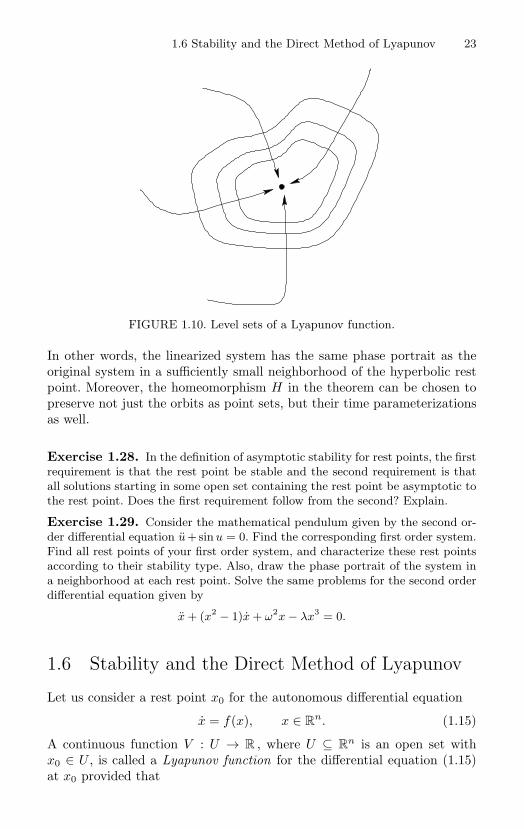
FIGURE 1.10. Level sets of a Lyapunov function.
In other words, the linearized system has the same phase portrait as theoriginal system in a sufficiently small neighborhood of the hyperbolic restpoint. Moreover, the homeomorphism H in the theorem can be chosen topreserve not just the orbits as point sets, but their time parameterizationsas well.
Exercise 1.28. In the definition of asymptotic stability for rest points, the firstrequirement is that the rest point be stable and the second requirement is thatall solutions starting in some open set containing the rest point be asymptotic tothe rest point. Does the first requirement follow from the second? Explain.
Exercise 1.29. Consider the mathematical pendulum given by the second or-der differential equation u+sin u = 0. Find the corresponding first order system.Find all rest points of your first order system, and characterize these rest pointsaccording to their stability type. Also, draw the phase portrait of the system ina neighborhood at each rest point. Solve the same problems for the second orderdifferential equation given by
x + (x2 − 1)x + ω2x − λx3 = 0.
1.6 Stability and the Direct Method of Lyapunov
Let us consider a rest point x0 for the autonomous differential equation
x = f(x), x ∈ Rn. (1.15)
A continuous function V : U → R , where U ⊆ Rn is an open set with
x0 ∈ U , is called a Lyapunov function for the differential equation (1.15)at x0 provided that
24 1. Introduction to Ordinary Differential Equations
(i) V (x0) = 0,
(ii) V (x) > 0 for x ∈ U − x0,
(iii) the function x → gradV (x) is continuous for x ∈ U − x0, and, onthis set, V (x) := gradV (x) · f(x) ≤ 0.
If, in addition,
(iv ) V (x) < 0 for x ∈ U − x0,
then V is called a strict Lyapunov function.
Theorem 1.30 (Lyapunov’s Stability Theorem). If x0 is a rest pointfor the differential equation (1.15) and V is a Lyapunov function for thesystem at x0, then x0 is stable. If, in addition, V is a strict Lyapunovfunction, then x0 is asymptotically stable.
The idea of Lyapunov’s method is very simple. In many cases the levelsets of V are “spheres” surrounding the rest point x0 as in Figure 1.10.Suppose this is the case and let φt denote the flow of the differential equa-tion (1.15). If y is in the level set Sc = x ∈ R
n : V (x) = c of the functionV , then, by the chain rule, we have that
d
dtV (φt(y))
∣∣∣t=0
= gradV (y) · f(y) ≤ 0. (1.16)
The vector grad V is an outer normal for Sc at y. (Do you see why it mustbe the outer normal?) Thus, V is not increasing on the curve t → φt(y) att = 0, and, as a result, the image of this curve either lies in the level setSc, or the set φt(y) : t > 0 is a subset of the set in the plane with outerboundary Sc. The same result is true for every point on Sc. Therefore, asolution starting on Sc is trapped; it either stays in Sc, or it stays in the setx ∈ R
n : V (x) < c. The stability of the rest point follows easily from thisresult. If V is a strict Lyapunov function, then the solution curve definitelycrosses the level set Sc and remains inside the set x ∈ R
n : V (x) < c forall t > 0. Because the same property holds at all level sets “inside” Sc, therest point x0 is asymptotically stable.
If the level sets of our Lyapunov function are as depicted in Figure 1.10,then the argument just given proves the stability of the rest point. How-ever, it is not clear that the level sets of a Lyapunov function must havethis simple configuration. For example, some of the level sets may not bebounded.
The proof of Lyapunov’s stability theorem requires a more delicate anal-ysis. Let us use the following notation. For α > 0 and ζ ∈ R
n, define
Sα(ζ) := x ∈ Rn : |x − ζ| = α,
Bα(ζ) := x ∈ Rn : |x − ζ| < α,
Bα(ζ) := x ∈ Rn : |x − ζ| ≤ α.
1.6 Stability and the Direct Method of Lyapunov 25
Proof. Suppose that ε > 0 is given, and note that, in view of the definitionof Lyapunov stability, it suffices to assume that Bε(x0) is contained inthe domain U of the Lyapunov function V . Using the fact that Sε(x0)is a compact set not containing x0, there is a number m > 0 such thatV (x) ≥ m for all x ∈ Sε(x0). Also, there is some δ > 0 with δ < ε suchthat the maximum value M of V on the compact set Bδ(x0) satisfies theinequality M < m. If not, consider the closed balls given by Bε/k(x0) fork ≥ 2, and extract a sequence of points xk∞
k=1 such that xk ∈ Bε/k(x0)and V (xk) ≥ m. Clearly, this sequence converges to x0. Using the continuityof the Lyapunov function V at x0, we have limk→∞ V (xk) = V (x0) = 0, incontradiction.
Let ϕt denote the flow of (1.15). If x ∈ Bδ(x0), then
d
dtV (ϕt(x)) = gradV (ϕt(x))f(ϕt(x)) ≤ 0.
Thus, the function t → V (ϕt(x)) is not increasing. Since V (ϕ0(x)) ≤ M <m, we must have V (ϕt(x)) < m for all t ≥ 0 for which the solution t →ϕt(x) is defined. But, for these values of t, we must also have ϕt(x) ∈Bε(x0). If not, there is some T > 0 such that |ϕT (x) − x0| ≥ ε. Sincet → |ϕt(x) − x0| is a continuous function, there must then be some τ with0 < τ ≤ T such that |ϕτ (x) − x0| = ε. For this τ , we have V (ϕτ (x)) ≥ m,in contradiction. Thus, ϕt(x) ∈ Bε(x0) for all t ≥ 0 for which the solutionthrough x exists. By the extensibility theorem, if the solution does not existfor all t ≥ 0, then |ϕt(x)| → ∞ as t → ∞, or ϕt(x) approaches the boundaryof the domain of definition of f . Since neither of these possibilities occur,the solution exists for all positive time with its corresponding image in theset Bε(x0). Thus, x0 is stable.
If, in addition, the Lyapunov function is strict, we will show that x0 isasymptotically stable.
Let x ∈ Bδ(x0). By the compactness of Bε(x0), either limt→∞ φt(x) = x0,or there is a sequence tk∞
k=1 of real numbers 0 < t1 < t2 · · · with tk → ∞such that the sequence ϕtk
(x)∞n=1 converges to some point x∗ ∈ Bε(x0)
with x∗ = x0. If x0 is not asymptotically stable, then such a sequence existsfor at least one point x ∈ Bδ(x0).
Using the continuity of V , it follows that limk→∞ V (ϕtk(x)) = V (x∗).
Also, V decreases on orbits. Thus, for each natural number k, we havethat V (ϕtk
(x)) > V (x∗). But, in view of the fact that the function t →V (φt(x∗)) is strictly decreasing, we have
limk→∞
V (ϕ1+tk(x)) = lim
k→∞V (ϕ1(ϕtk
(x))) = V (ϕ1(x∗)) < V (x∗).
Thus, there is some natural number such that V (φ1+t(x)) < V (x∗).
Clearly, there is also an integer n > such that tn > 1 + t. For thisinteger, we have the inequalities V (φtn(x)) < V (φ1+t
(x)) < V (x∗), incontradiction.
26 1. Introduction to Ordinary Differential Equations
Example 1.31. The linearization of x = −x3 at x = 0 is x = 0. It providesno information about stability. Define V (x) = x2 and note that V (x) =2x(−x3) = −2x4. Thus, V is a strict Lyapunov function, and the rest pointat x = 0 is asymptotically stable.
Example 1.32. Consider the harmonic oscillator x+ω2x = 0 with ω > 0.The equivalent first order system
x = y, y = −ω2x
has a rest point at (x, y) = (0, 0). Define the total energy (kinetic energyplus potential energy) of the harmonic oscillator to be
V =12x2 +
ω2
2x2 =
12(y2 + ω2x2).
A computation shows that V = 0. Thus, the rest point is stable. The energyof a physical system is often a good choice for a Lyapunov function!
Exercise 1.33. As a continuation of example (1.32), consider the equivalentfirst order system
x = ωy, y = −ωx.
Study the stability of the rest point at the origin using Lyapunov’s direct method.
Exercise 1.34. Consider a Newtonian particle of mass m moving under theinfluence of the potential U . If the position coordinate is denoted by
q = (q1, . . . , qn),
then the equation of motion (F = ma) is given by
mq = − grad U(q).
If q0 is a strict local minimum of the potential, show that the equilibrium (q, q) =(0, q0) is Lyapunov stable. Hint: Consider the total energy of the particle.
Exercise 1.35. Determine the stability of the rest points of the following sys-tems. Formulate properties of the unspecified scalar function g so that the restpoint at the origin is stable or asymptotically stable.
1. x = y − x3,
y = −x − y3
2. x = y + αx(x2 + y2),y = −x + αy(x2 + y2)
3. x = 2xy − x3,
y = −x2 − y5
4. x = y − xg(x, y),y = −x − yg(x, y)
1.6 Stability and the Direct Method of Lyapunov 27
5. x = y + xy2 − x3 + 2xz4,
y = −x − y3 − 3x2y + 3yz4,
z = − 52y2z3 − 2x2z3 − 1
2z7
Exercise 1.36. Determine the stability of all rest points for the following dif-ferential equations. For the unspecified scalar function g determine conditions sothat the origin is a stable and/or asymptotically stable rest point.
1. x + εx + ω2x = 0, ε > 0, ω > 0
2. x + sin x = 0
3. x + x − x3 = 0
4. x + g(x) = 0
5. x + εx + g(x) = 0, ε > 0
6. x + x3 + x = 0.
The total energy is a good choice for the strict Lyapunov function required tostudy system 5. It almost works. Can you modify the total energy to obtain astrict Lyapunov function? If not, see Exercise 2.45. Alternatively, consider apply-ing the following refinement of Theorem 1.30: Suppose that x0 is a rest point forthe differential equation x = f(x) with flow φt and V is a Lyapunov function atx0. If, in addition, there is a neighborhood W of the rest point x0 such that foreach point p ∈ W \x0, the function V is not constant on the set φt(p) : t ≥ 0,then x0 is asymptotically stable (see Exercise 1.113).
Exercise 1.37. [Basins of Attraction] Consider system 5 in the previous exer-cise, and note that if g(0) = 0 and g′(0) > 0, then there is a rest point at the originthat is asymptotically stable. Moreover, this fact can be proved by the principleof linearization. Thus, it might seem that finding a strict Lyapunov function inthis case is wasted effort. However, the existence of a strict Lyapunov functiondetermines more than just the stability of the rest point; the Lyapunov functioncan also be used to estimate the basin of attraction of the rest point; that is (ingeneral), the set of all points in the space that are asymptotic to the rest point.Consider the (usual) first order system corresponding to the differential equation
x + εx + x − x3 = 0
for ε > 0, and describe the basin of attraction of the origin. Define a subset ofthe basin of attraction, which you have described, and prove that it is containedin the basin of attraction. Formulate and prove a general theorem about theexistence of Lyapunov functions and the extent of basins of attraction of restpoints.
In engineering practice, physical systems (for example a chemical plant or apower electronic system) are operated in steady state. When a disturbance occursin the system, the control engineer wants to know if the system will return tothe steady state. If not, she will have to take drastic action! Do you see whytheorems of the type requested in this exercise (a possible project for the rest ofyour mathematical life) would be of practical value?
Exercise 1.38. Prove the following instability result: Suppose that V is asmooth function defined on an open neighborhood U of the rest point x0 of
28 1. Introduction to Ordinary Differential Equations
the autonomous system x = f(x) such that V (x0) = 0 and V (x) > 0 on U \x0.If for each neighborhood of x0 there is a point where V has a positive value, thenx0 is not stable.
1.7 Introduction to Invariant Manifolds
In this section we will define the concept of a manifold as a generalizationof a linear subspace of R
n, and we will begin our discussion of the centralrole that manifolds play in the theory of differential equations.
Let us note that the fundamental definitions of the calculus are local innature. For example, the derivative of a function at a point is determinedonce we know the values of the function in some neighborhood of the point.This fact is the basis for the manifold concept: Informally, a manifold is asubset of R
n such that, for some fixed integer k ≥ 0, each point in the subsethas a neighborhood that is essentially the same as the Euclidean spaceR
k. To make this definition precise we will have to define what is meantby a neighborhood in the subset, and we will also have to understand themeaning of the phrase “essentially the same as R
k.” However, these notionsshould be intuitively clear: In effect, a neighborhood in the manifold is anopen subset that is diffeomorphic to R
k.Points, lines, planes, arcs, spheres, and tori are examples of manifolds.
Some of these manifolds have already been mentioned. Let us recall that acurve is a smooth function from an open interval of real numbers into R
n.An arc is the image of a curve. Every solution of a differential equation is acurve; the corresponding orbit is an arc. Thus, every orbit of a differentialequation is a manifold. As a special case, let us note that a periodic orbitis a one-dimensional torus.
Consider the differential equation
x = f(x), x ∈ Rn, (1.17)
with flow φt, and let S be a subset of Rn that is a union of orbits of this
flow. If a solution has its initial condition in S, then the corresponding orbitstays in S for all time, past and future. The concept of a set that is theunion of orbits of a differential equation is formalized in the next definition.
Definition 1.39. A set S ⊆ Rn is called an invariant set for the differen-
tial equation (1.17) if, for each x ∈ S, the solution t → φt(x), defined on itsmaximal interval of existence, has its image in S. Alternatively, the orbitpassing through each x ∈ S lies in S. If, in addition, S is a manifold, thenS is called an invariant manifold.
We will illustrate the notion of invariant manifolds for autonomous dif-ferential equations by describing two important examples: the stable, un-stable, and center manifolds of a rest point; and the energy surfaces ofHamiltonian systems.
1.7 Introduction to Invariant Manifolds 29
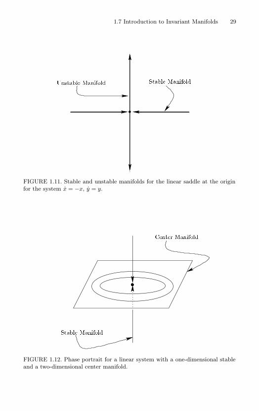
Stable ManifoldUnstable Manifold
FIGURE 1.11. Stable and unstable manifolds for the linear saddle at the originfor the system x = −x, y = y.
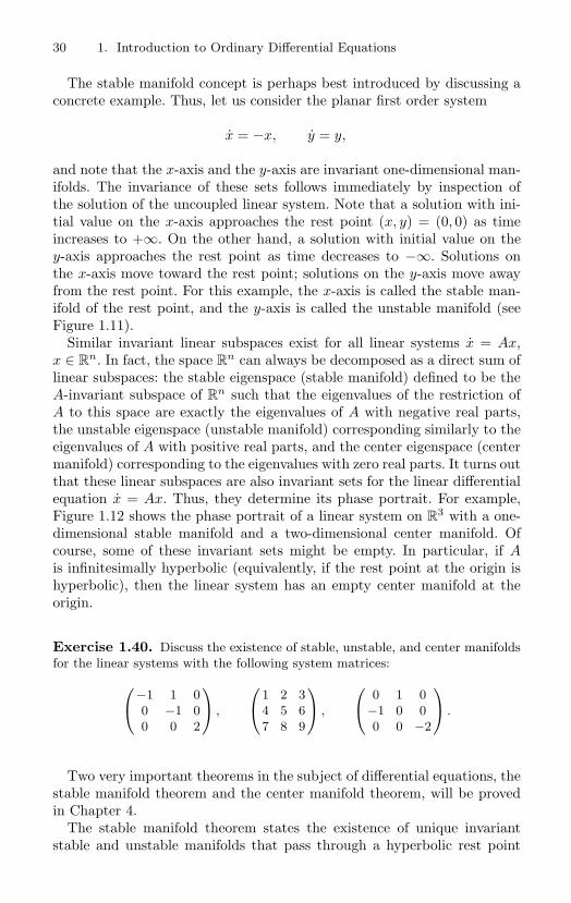
Center Manifold
Stable Manifold
FIGURE 1.12. Phase portrait for a linear system with a one-dimensional stableand a two-dimensional center manifold.
30 1. Introduction to Ordinary Differential Equations
The stable manifold concept is perhaps best introduced by discussing aconcrete example. Thus, let us consider the planar first order system
x = −x, y = y,
and note that the x-axis and the y-axis are invariant one-dimensional man-ifolds. The invariance of these sets follows immediately by inspection ofthe solution of the uncoupled linear system. Note that a solution with ini-tial value on the x-axis approaches the rest point (x, y) = (0, 0) as timeincreases to +∞. On the other hand, a solution with initial value on they-axis approaches the rest point as time decreases to −∞. Solutions onthe x-axis move toward the rest point; solutions on the y-axis move awayfrom the rest point. For this example, the x-axis is called the stable man-ifold of the rest point, and the y-axis is called the unstable manifold (seeFigure 1.11).
Similar invariant linear subspaces exist for all linear systems x = Ax,x ∈ R
n. In fact, the space Rn can always be decomposed as a direct sum of
linear subspaces: the stable eigenspace (stable manifold) defined to be theA-invariant subspace of R
n such that the eigenvalues of the restriction ofA to this space are exactly the eigenvalues of A with negative real parts,the unstable eigenspace (unstable manifold) corresponding similarly to theeigenvalues of A with positive real parts, and the center eigenspace (centermanifold) corresponding to the eigenvalues with zero real parts. It turns outthat these linear subspaces are also invariant sets for the linear differentialequation x = Ax. Thus, they determine its phase portrait. For example,Figure 1.12 shows the phase portrait of a linear system on R
3 with a one-dimensional stable manifold and a two-dimensional center manifold. Ofcourse, some of these invariant sets might be empty. In particular, if Ais infinitesimally hyperbolic (equivalently, if the rest point at the origin ishyperbolic), then the linear system has an empty center manifold at theorigin.
Exercise 1.40. Discuss the existence of stable, unstable, and center manifoldsfor the linear systems with the following system matrices:
−1 1 0
0 −1 00 0 2
,
1 2 3
4 5 67 8 9
,
0 1 0
−1 0 00 0 −2
.
Two very important theorems in the subject of differential equations, thestable manifold theorem and the center manifold theorem, will be provedin Chapter 4.
The stable manifold theorem states the existence of unique invariantstable and unstable manifolds that pass through a hyperbolic rest point
1.7 Introduction to Invariant Manifolds 31
tangent to the corresponding stable and unstable eigenspaces of the corre-sponding linearized system. Let us note that the Hartman–Grobman theo-rem implies that a hyperbolic rest point has stable and unstable invariantsets that are homeomorphic images of the corresponding invariant man-ifolds for the corresponding linearized system, but it gives no indicationthat these invariant sets are smooth manifolds.
The existence of stable and unstable invariant manifolds is important.However, at this point in our study only a glimpse into their essential role inthe analysis of differential equations is possible. For example, their existenceprovides a theoretical basis for determining the analytic properties of theflow of a differential equation in the neighborhood of a hyperbolic restpoint. They also serve to bound other invariant regions in the phase space.Thus, the network of all stable and unstable manifolds forms the “skeleton”for the phase portrait. Finally, the existence of the stable and unstablemanifolds in the phase space, especially their intersection properties, liesat the heart of an explanation of the complex motions associated with manynonlinear ordinary differential equations. In particular, this phenomenon isfundamental in the study of deterministic chaos (see Chapter 6).
For rest points of a differential equation that are not hyperbolic, the cen-ter manifold theorem states the existence of an invariant manifold tangentto the corresponding center eigenspace. This center manifold is not nec-essarily unique, but the differential equation has the same phase portraitwhen restricted to any one of the center manifolds at the same rest point.Analysis using center manifolds is often required to understand many ofthe most delicate problems that arise in the theory and applications ofdifferential equations. For example, the existence and smoothness proper-ties of center manifolds are foundational results in bifurcation theory (seeChapter 8).
Invariant manifolds, called energy surfaces, are useful in the study ofHamiltonian systems of differential equations. To define this importantclass of differential equations, let H : R
n × Rn → R be a smooth func-
tion given by
(q1, . . . , qn, p1, . . . , pn) → H(q1, . . . , qn, p1, . . . , pn),
and define the associated Hamiltonian system on R2n with Hamiltonian H
by
qi =∂H
∂pi, pi = −∂H
∂qi, i = 1, . . . , n.
Let us note that the dimension of the phase space of a Hamiltonian systemis required to be even. The reason for this restriction will soon be madeclear.
As a prototypical example of a Hamiltonian system, let H : R2 → R be
given by H(x, y) := 12 (y2 + ω2x2). The associated Hamiltonian system is
32 1. Introduction to Ordinary Differential Equations
the harmonic oscillator
x = y, y = −ω2x.
More generally, suppose that U : Rn → R and let H : R
n × Rn → R be
given by
H(q, p) =p2
2m+ U(q)
where p2 := p21 + · · · + p2
n. A Hamiltonian in this form is called a classicalHamiltonian. The corresponding Hamiltonian system
q =1m
p, p = − gradU(q)
is equivalent to Newton’s equation of motion for a particle influenced bya conservative force (see Exercise 1.34). The vector quantity p := mq iscalled the (generalized) momentum, the function U is called the potentialenergy, and the function p → 1
2mp2 = m2 q2 is called the kinetic energy.
The configuration space for the classical mechanical system is the spaceconsisting of all possible positions of the system. If the configuration space islocally specified by n coordinates (q1, . . . , qn), then the Hamiltonian systemis said to have n degrees of freedom. For example, for the pendulum, theconfiguration space can be taken to be R with the coordinate q1 specifyingthe angular position of the bob relative to the downward vertical. It is asystem with one degree of freedom. Of course, for this example, the physicalpositions are specified by the angular coordinate q1 modulo 2π. Thus, theconfiguration space can also be viewed as a nonlinear manifold—namely,the unit circle in the plane. This is yet another way in which manifoldsarise in the study of mechanical systems.
The phase space of a Hamiltonian system is the subset of Rn × R
n of allpositions and momenta specified by the coordinates (q1, . . . , qn, p1, . . . , qn).The dimension of the phase space is therefore even; it is the space in whichthe Hamiltonian system evolves. The state space is also a subset of R
n ×R
n, but it is the space of positions and velocities with the coordinates(q1, . . . , qn, q1, . . . , qn) (see Chapter 3).
For c ∈ R and the Hamiltonian H : Rn × R
n → R, the correspondingenergy surface with energy c is defined to be the set
Sc = (q, p) ∈ Rn × R
n : H(q, p) = c.
If gradH(p, q) = 0 for each (p, q) ∈ Sc, then the set Sc is called a regularenergy surface.
Note that the vector field given by
gradH = (∂H
∂q,∂H
∂p)
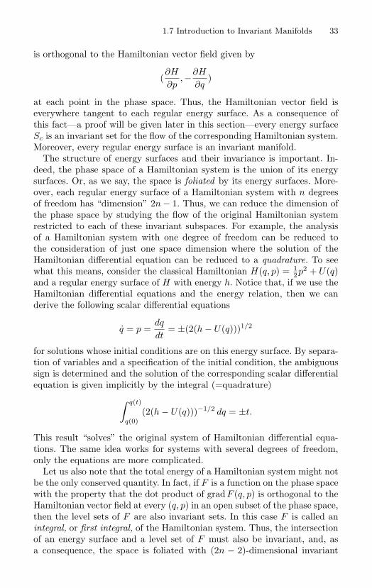
1.7 Introduction to Invariant Manifolds 33
is orthogonal to the Hamiltonian vector field given by
(∂H
∂p,−∂H
∂q)
at each point in the phase space. Thus, the Hamiltonian vector field iseverywhere tangent to each regular energy surface. As a consequence ofthis fact—a proof will be given later in this section—every energy surfaceSc is an invariant set for the flow of the corresponding Hamiltonian system.Moreover, every regular energy surface is an invariant manifold.
The structure of energy surfaces and their invariance is important. In-deed, the phase space of a Hamiltonian system is the union of its energysurfaces. Or, as we say, the space is foliated by its energy surfaces. More-over, each regular energy surface of a Hamiltonian system with n degreesof freedom has “dimension” 2n − 1. Thus, we can reduce the dimension ofthe phase space by studying the flow of the original Hamiltonian systemrestricted to each of these invariant subspaces. For example, the analysisof a Hamiltonian system with one degree of freedom can be reduced tothe consideration of just one space dimension where the solution of theHamiltonian differential equation can be reduced to a quadrature. To seewhat this means, consider the classical Hamiltonian H(q, p) = 1
2p2 + U(q)and a regular energy surface of H with energy h. Notice that, if we use theHamiltonian differential equations and the energy relation, then we canderive the following scalar differential equations
q = p =dq
dt= ±(2(h − U(q)))1/2
for solutions whose initial conditions are on this energy surface. By separa-tion of variables and a specification of the initial condition, the ambiguoussign is determined and the solution of the corresponding scalar differentialequation is given implicitly by the integral (=quadrature)∫ q(t)
q(0)(2(h − U(q)))−1/2 dq = ±t.
This result “solves” the original system of Hamiltonian differential equa-tions. The same idea works for systems with several degrees of freedom,only the equations are more complicated.
Let us also note that the total energy of a Hamiltonian system might notbe the only conserved quantity. In fact, if F is a function on the phase spacewith the property that the dot product of gradF (q, p) is orthogonal to theHamiltonian vector field at every (q, p) in an open subset of the phase space,then the level sets of F are also invariant sets. In this case F is called anintegral, or first integral, of the Hamiltonian system. Thus, the intersectionof an energy surface and a level set of F must also be invariant, and, asa consequence, the space is foliated with (2n − 2)-dimensional invariant
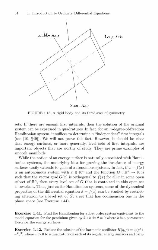
34 1. Introduction to Ordinary Differential Equations
Middle Axis
Short Axis
Long Axis
FIGURE 1.13. A rigid body and its three axes of symmetry
sets. If there are enough first integrals, then the solution of the originalsystem can be expressed in quadratures. In fact, for an n-degree-of-freedomHamiltonian system, it suffices to determine n “independent” first integrals(see [10, §49]). We will not prove this fact. However, it should be clearthat energy surfaces, or more generally, level sets of first integrals, areimportant objects that are worthy of study. They are prime examples ofsmooth manifolds.
While the notion of an energy surface is naturally associated with Hamil-tonian systems, the underlying idea for proving the invariance of energysurfaces easily extends to general autonomous systems. In fact, if x = f(x)is an autonomous system with x ∈ R
n and the function G : Rn → R is
such that the vector grad G(x) is orthogonal to f(x) for all x in some opensubset of R
n, then every level set of G that is contained in this open setis invariant. Thus, just as for Hamiltonian systems, some of the dynamicalproperties of the differential equation x = f(x) can be studied by restrict-ing attention to a level set of G, a set that has codimension one in thephase space (see Exercise 1.44).
Exercise 1.41. Find the Hamiltonian for a first order system equivalent to themodel equation for the pendulum given by θ+k sin θ = 0 where k is a parameter.Describe the energy surfaces.
Exercise 1.42. Reduce the solution of the harmonic oscillator H(q, p) = 12 (p2+
ω2q2) where ω > 0 to a quadrature on each of its regular energy surfaces and carry
1.7 Introduction to Invariant Manifolds 35
out the integration explicitly. (This is not the simplest way to solve the equationsof motion, but you will learn a valuable method that is used, for example, in theconstruction of the solution of the equations of motion for the Hamiltonian systemmentioned in the previous exercise.)
Exercise 1.43. [Gradient Systems] If H is a Hamiltonian, then the vector fieldgrad H is everywhere orthogonal to the corresponding Hamiltonian vector field.However, the vector field grad H defines a differential equation in its own rightthat has many interesting and useful properties. More generally, for a smoothfunction G : R
n → R (maybe n is odd), let us define the associated gradientsystem
x = grad G(x).
Because a conservative force is the negative gradient of a potential, many authorsdefine the gradient system with potential G to be
x = − grad G(x).
While our definition is the usual one for mathematical studies, the definitionwith the negative sign is perhaps more natural for physical applications. Provethe following facts: A gradient system has no periodic orbits. If a gradient systemhas a rest point, then all of the eigenvalues of the linearization at the rest point arereal. If n = 2, then the orbits of the gradient system are orthogonal trajectoriesfor the orbits of the Hamiltonian system with Hamiltonian G. If x ∈ R
n is anisolated maximum of the function G : R
n → R, then x is an asymptotically stablerest point of the corresponding gradient system.
Exercise 1.44. [Rigid Body Motion] A system that is not Hamiltonian, butclosely related to this class, is given by Euler’s equations for rigid body motion.The angular momentum M = (M1, M2, M3) of a rigid body, relative to a coordi-nate frame rotating with the body with axes along the principal axes of the bodyand with origin at its center of mass, is related to the angular velocity vector Ωby M = AΩ, where A is a symmetric matrix called the inertia matrix. Euler’sequation is M = M × Ω. Equivalently, the equation for the angular velocity isAΩ = (AΩ) × Ω. If A is diagonal with diagonal components (moments of iner-tia) (I1, I2, I3), show that Euler’s equations for the components of the angularmomentum are given by
M1 = −( 1I2
− 1I3
)M2M3,
M2 =( 1I1
− 1I3
)M1M3,
M3 = −( 1I1
− 1I2
)M1M2.
Assume that 0 < I1 ≤ I2 ≤ I3. Find some invariant manifolds for this system. Canyou use your results to find a qualitative description of the motion? As a physicalexample, take this book and hold its covers together with a rubber band. Then,toss the book vertically three times, imparting a rotation in turn about each ofits axes of symmetry (see Figure 1.13). Are all three rotary motions Lyapunovstable? Do you observe any other interesting phenomena associated with the
36 1. Introduction to Ordinary Differential Equations
motion? For example, pay attention to the direction of the front cover of thebook after each toss. Hint: Look for invariant quadric surfaces; that is, manifoldsdefined as level sets of quadratic polynomials (first integrals) in the variables(M1, M2, M3). For example, show that the kinetic energy given by 1
2 〈AΩ, Ω〉is constant along orbits. The total angular momentum (length of the angularmomentum) is also conserved. For a complete mathematical description of rigidbody motion, see [10]. For a mathematical description of the observed “twist”in the rotation of the tossed book, see [16]. One aspect of this problem worthmentioning is the fact that Euler’s equations do not describe the motion of thebook in space. To do so would require a functional relationship between thecoordinate system rotating with the body and the position coordinates relativeto a fixed coordinate frame in space.
1.7.1 Smooth ManifoldsBecause the modern definition of a smooth manifold can appear quiteformidable at first sight, we will formulate a simpler equivalent definitionfor the class of manifolds called the submanifolds of R
n. Fortunately, thisclass is rich enough to contain the manifolds that are met most often in thestudy of differential equations. In fact, every manifold can be “embedded”as a submanifold of some Euclidean space. Thus, the class that we willstudy can be considered to contain all manifolds.
Recall that a manifold is supposed to be a set that is locally the same asR
k. Thus, whatever is meant by “locally the same,” every open subset ofR
k must be a manifold.If W ⊆ R
k is an open set and g : W → Rn−k is a smooth function, then
the graph of g is the subset of Rn defined by
graph(g) := (w, g(w)) ∈ Rn : w ∈ W.
The set graph(g) is the same as W ⊆ Rk up to a nonlinear change of
coordinates. By this we mean that there is a smooth map G with domainW and image graph(g) such that G has a smooth inverse. In fact, such amap G : W → graph(g) is given by G(w) = (w, g(w)). Clearly, G is smooth.Its inverse is the linear projection on the first k coordinates of the point(w, g(w)) ∈ graph(g); that is, G−1(w, g(w)) = w. Thus, G−1 is smooth aswell.
Open subsets and graphs of smooth functions are the prototypical exam-ples of what we will call submanifolds. However, these classes are too re-strictive; they include objects that are in fact globally the same as some Eu-clidean space. The unit circle T in the plane, also called the one-dimensionaltorus, is an example of a submanifold that is not of this type. Indeed,T := (x, y) : x2 + y2 = 1 is not the graph of a scalar function defined onan open subset of R. However, every point of T is contained in a neighbor-hood in T that is the graph of such a function. In fact, each point in T is
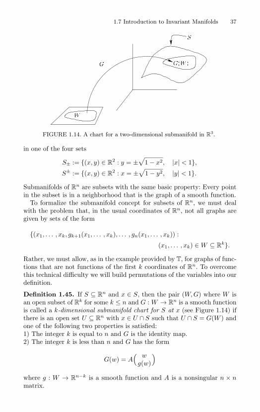
1.7 Introduction to Invariant Manifolds 37
GW
W
S
G
FIGURE 1.14. A chart for a two-dimensional submanifold in R3.
in one of the four sets
S± := (x, y) ∈ R2 : y = ±
√1 − x2, |x| < 1,
S± := (x, y) ∈ R2 : x = ±
√1 − y2, |y| < 1.
Submanifolds of Rn are subsets with the same basic property: Every point
in the subset is in a neighborhood that is the graph of a smooth function.To formalize the submanifold concept for subsets of R
n, we must dealwith the problem that, in the usual coordinates of R
n, not all graphs aregiven by sets of the form
(x1, . . . , xk, gk+1(x1, . . . , xk), . . . , gn(x1, . . . , xk)) :
(x1, . . . , xk) ∈ W ⊆ Rk.
Rather, we must allow, as in the example provided by T, for graphs of func-tions that are not functions of the first k coordinates of R
n. To overcomethis technical difficulty we will build permutations of the variables into ourdefinition.
Definition 1.45. If S ⊆ Rn and x ∈ S, then the pair (W, G) where W is
an open subset of Rk for some k ≤ n and G : W → R
n is a smooth functionis called a k-dimensional submanifold chart for S at x (see Figure 1.14) ifthere is an open set U ⊆ R
n with x ∈ U ∩ S such that U ∩ S = G(W ) andone of the following two properties is satisfied:1) The integer k is equal to n and G is the identity map.2) The integer k is less than n and G has the form
G(w) = A( w
g(w)
)where g : W → R
n−k is a smooth function and A is a nonsingular n × nmatrix.
38 1. Introduction to Ordinary Differential Equations
Definition 1.46. The set S ⊆ Rn is called a k-dimensional smooth sub-
manifold of Rn if there is a k-dimensional submanifold chart for S at every
point x in S.
If (W, G) is a submanifold coordinate chart, then the map G is called asubmanifold coordinate map. If S is a submanifold of R
n, then, even thoughwe have not defined the concept, let us also call S a smooth manifold.
As an example, let us show that T is a one-dimensional manifold. Con-sider a point in the subset S+ = (x, y) : x =
√1 − y2, |y| < 1 of T. Define
the set W := t ∈ R : |t| < 1, the function g : W → R by g(t) =√
1 − t2,the set U := (x, y) ∈ R
2 : (x − 1)2 + y2 <√
2, and the matrix
A :=(
0 11 0
).
Then we have
T ∩ U =(x
y
)∈ R
2 :(x
y
)=
(0 11 0
)(t
g(t)
), t ∈ W
.
Similarly, T is locally the graph of a smooth function at points in the subsetsS− and S±, as required.
A simple but important result about submanifold coordinate charts isthe following proposition.
Proposition 1.47. If (W, G) is a submanifold coordinate chart for a k-dimensional submanifold of R
n, then the function G : W → S is invertible.Moreover, the inverse of G is the restriction of a smooth function that isdefined on all of R
n.
Proof. The result is obvious if k = n. If k < n, then define Π : Rn → R
k tobe the linear projection on the first k-coordinates; that is, Π(x1, . . . , xn) =(x1, . . . , xk), and define
F : G(W ) → W
byF (s) = ΠA−1s.
Clearly, F is smooth as a function defined on all of Rn. Also, if w ∈ W ,
then
F G(w) = F(A(
wg(w)
))= ΠA−1A
( wg(w)
)= w.
If s ∈ G(W ), then s = A(
wg(w)
)for some w ∈ W . Hence, we also have
G(F (s)) = G(w) = s.
This proves that F is the inverse of G.
1.7 Introduction to Invariant Manifolds 39
If S is a submanifold, then we can use the submanifold coordinate chartsto define the open subsets of S.
Definition 1.48. If S is a submanifold, then the open subsets of S are allpossible unions of all sets of the form G(W ) where (W, G) is a submanifoldchart for S.
The next proposition is an immediate consequence of the definitions.
Proposition 1.49. If S is a submanifold of Rn and if V is an open subset
of S, then there is an open set U of Rn such that V = S ∩ U ; that is, the
topology defined on S using the submanifold charts agrees with the subspacetopology on S.
As mentioned above, one of the main reasons for defining the manifoldconcept is to distinguish those subsets of R
n on which we can use thecalculus. To do so, let us first make precise the notion of a smooth function.
Definition 1.50. Suppose that S1 is a submanifold of Rm, S2 is a subman-
ifold of Rn, and F is a function F : S1 → S2. We say that F is differentiable
at x1 ∈ S1 if there are submanifold coordinate charts (W1, G1) at x1 and(W2, G2) at F (x1) such that the map G−1
2 F G1 : W1 → W2 is differ-entiable at G−1
1 (x1) ∈ W1. If F is differentiable at each point of an opensubset V of S1, then we say that F is differentiable on V .
Definition 1.51. Suppose that S1 and S2 are manifolds. A smooth func-tion F : S1 → S2 is called a diffeomorphism if there is a smooth functionH : S2 → S1 such that H(F (s)) = s for every s ∈ S1 and F (H(s)) = s forevery s ∈ S2. The function H is called the inverse of F and is denoted byF−1.
With respect to the notation in Definition 1.50, we have defined theconcept of differentiability for the function F : S1 → S2, but we have notyet defined what we mean by its derivative! However, we have determinedthe derivative relative to the submanifold coordinate charts used in thedefinition. Indeed, the local representative of the function F is given byG−1
2 F G1, a function defined on an open subset of a Euclidean space withrange in another Euclidean space. By definition, the local representative ofthe derivative of F relative to the given submanifold charts is the usualderivative in Euclidean space of this local representative of F . In the nextsubsection, we will interpret the derivative of F without regard to the choiceof a submanifold coordinate chart; that is, we will give a coordinate-freedefinition of the derivative of F (see also Exercise 1.52).
Exercise 1.52. Prove: The differentiability of a function defined on a manifolddoes not depend on the choice of submanifold coordinate chart.
40 1. Introduction to Ordinary Differential Equations
We have used the phrase “smooth function” to refer to a function that iscontinuously differentiable. In view of Definition 1.50, the smoothness of afunction defined on a manifold is determined by the smoothness of its localrepresentatives—functions that are defined on open subsets of Euclideanspaces. It is clear that smoothness of all desired orders can be defined inthe same manner by imposing the requirement on local representatives.More precisely, if F is a function defined on a manifold S, then we willsay that F is an element of Cr(S), for r a nonnegative integer, r = ∞,or r = ω, provided that at each point of S there is a local representativeof F all of whose partial derivatives up to and including those of order rare continuous. If r = ∞, then all partial derivatives are required to becontinuous. If r = ω, then all local representatives are all required to haveconvergent power series representations valid in a neighborhood of eachpoint of their domains. A function in Cω is called real analytic.
In the subject of differential equations, specifying the minimum numberof derivatives of a function required to obtain a result often obscures themain ideas that are being illustrated. Thus, as a convenient informality,we will often use the phrase “smooth function” to mean that the functionin question has as many continuous derivatives as needed. However, thereare instances where the exact requirement for the number of derivativesis essential. In these cases, we will refer to the appropriate class of Cr
functions.The next definition formalizes the concept of a coordinate system.
Definition 1.53. Suppose that S is a k-dimensional submanifold. If Vis an open subset of S, W is an open subset of R
k, and Ψ : V → Wis a diffeomorphism, then the pair (V, Ψ) is called a coordinate system orcoordinate chart on S.
Exercise 1.54. Prove: If (W, G) is a submanifold coordinate chart for a man-ifold S, then (G(W ), G−1) is a coordinate chart on S.
The abstract definition of a manifold is based on the concept of coordi-nate charts. Informally, a set S together with a collection of subsets S isdefined to be a k-dimensional manifold if every point of S is contained in atleast one set in S and if, for each member V of S, there is a correspondingopen subset W of R
k and a function Ψ : V → W that is bijective. If twosuch subsets V1 and V2 overlap, then the domain of the map
Ψ1 Ψ−12 : Ψ2(V1 ∩ V2) → W1
is an open subset of Rk whose range is contained in an open subset of
Rk. The set S is called a manifold provided that all such “overlap maps”
are smooth (see [92] for the formal definition). This abstract notion of amanifold has the advantage that it does not require a manifold to be asubset of a Euclidean space.
1.7 Introduction to Invariant Manifolds 41
Exercise 1.55. Prove: If F : Rm → R
n is smooth and F (S1) ⊆ S2 for subman-ifolds S1 and S2, then the restriction of F to S1 is differentiable.
Exercise 1.56. Prove: If α ∈ R, then the map T → T given by
(x, y) → (x cos α − y sin α, x sin α + y cos α)
is a diffeomorphism.
Now that we know the definition of a manifold, we are ready to provethat linear subspaces of R
n and regular level sets of smooth functions aremanifolds.
Proposition 1.57. A linear subspace of Rn is a submanifold.
Proof. Let us suppose that S is the span of the k linearly independent vec-tors v1, . . . , vk in R
n. We will show that S is a k-dimensional submanifoldof R
n.Let e1, . . . , en denote the standard basis of R
n. By a basic result fromlinear algebra, there is a set consisting of n − k standard basis vectorsfk+1, . . . , fn such that the vectors
v1, . . . , vk, fk+1, . . . , fn
are a basis for Rn. (Why?) Let us denote the remaining set of standard
basis vectors by f1, . . . , fk. For each j = 1, . . . , k, there are scalars λji and
µji such that
fj =k∑
i=1
λjivi +
n∑i=k+1
µjifi.
Hence, if (t1, . . . , tk) ∈ Rk, then the vector
k∑j=1
tjfj −k∑
j=1
tj
( n∑i=k+1
µjifi
)=
k∑j=1
tj
( k∑i=1
λjivi
)is in S. Hence, relative to the basis f1, · · · , fn, the vector
(t1, . . . , tk,−k∑
j=1
tjµjk+1, . . . ,−
k∑j=1
tjµjn)
is in S.Define g : R
k → Rn−k by
g(t1, . . . , tk) :=(
−k∑
j=1
tjµjk+1, . . . ,−
k∑j=1
tjµjn
)
42 1. Introduction to Ordinary Differential Equations
and let A denote the permutation matrix that maps the vectors f1, . . . , fn
to their standard order e1, . . . , en; that is, Afi = ei for i = 1, . . . , n. Itfollows that the pair (Rk, G), where G : R
k → Rn is defined by
G(w) = A( w
g(w)
),
is a k-dimensional submanifold chart such that G(Rk) = Rn ∩ S. In fact,
by the construction, it is clear that the image of G is a linear subspace ofS. Moreover, because the image of G has dimension k as a vector space,the subspace G(Rk) is equal to S.
As mentioned previously, linear subspaces often arise as invariant mani-folds of differential equations. For example, consider the differential equa-tion given by x = Ax where x ∈ R
n and A is an n × n matrix. If S isan invariant subspace for the matrix A, for example, one of its generalizedeigenspaces, then, by Proposition 1.57, S is a submanifold of R
n. Also, S isan invariant set for the linear system of differential equations. A completeproof of this proposition requires some results from linear systems theorythat will be presented in Chapter 2. However, the essential features of theproof can be simply illustrated in the special case where the linear trans-formation A restricted to S has a complete set of eigenvectors. In otherwords, S is a k-dimensional subspace of R
n spanned by k linearly indepen-dent eigenvectors v1, . . . , vk of A. Under this assumption, if Avi = λivi,then t → eλitvi is a solution of x = Ax. Also, note that eλitvi is an eigen-vector of A for each t ∈ R. Therefore, if x0 ∈ S, then there are scalars(a1, . . . , ak) such that x0 =
∑ki=1 aivi and
t →k∑
i=1
eλitaivi
is the solution of the ordinary differential equation with initial conditionx(0) = x0. Clearly, the corresponding orbit stays in S for all t ∈ R.
Linear subspaces can be invariant sets for nonlinear differential equations.For example, consider the Volterra–Lotka system
x = x(a − by), y = y(cx − d).
In case a, b, c, and d are all positive, this system models the interactionof the population y of a predator and the population x of its prey. Forthis system, the x-axis and the y-axis are each invariant sets. Indeed, sup-pose that (0, y0) is a point on the y-axis corresponding to a population ofpredators with no prey, then t → (0, e−dty0) is the solution of the systemstarting at this point that models this population for all future time. Thissolution stays on the y-axis for all time, and, as there are is no spontaneousgeneration of prey, the predator population dies out in positive time.
1.7 Introduction to Invariant Manifolds 43
Let us now discuss level sets of functions. Recall that if H : Rn → R is a
smooth function, then the level set of H with energy c is the set
Sc := x ∈ Rn : H(x) = c.
Moreover, if gradH(x) = 0 for each x ∈ Sc, then Sc is called a regular levelset.
Proposition 1.58. If H : Rn → R is a smooth function, then each of its
regular level sets is an (n − 1)-dimensional submanifold of Rn.
It is instructive to outline a proof of this result because it provides ourfirst application of a nontrivial and very important theorem from advancedcalculus, namely, the implicit function theorem.
Suppose that Sc is a regular level set of H, choose a ∈ Sc, and defineF : R
n → R byF (x) = H(x) − c.
Let us note that F (a) = 0. Also, because gradH(a) = 0, there is at least oneinteger 1 ≤ i ≤ n such that the corresponding partial derivative ∂F/∂xi
does not vanish when evaluated at a. For notational convenience let ussuppose that i = 1. All other cases can be proved in a similar manner.
We are in a typical situation: We have a function F : R × Rn−1 → R
given by (x1, x2, . . . , xn) → F (x1, . . . , xn) such that
F (a1, . . . , an) = 0,∂F
∂x1(a1, a2, . . . , an) = 0.
This calls for an application of the implicit function theorem. A preliminaryversion of the theorem is stated here; a more general version will be provedlater (see Theorem 1.182).
If f : R × R
m → Rn is given by (p, q) → f(p, q), then, for fixed b ∈ R
m,consider the function R
→ Rn defined by p → f(p, b). Its derivative at
a ∈ R will be denoted by fp(a, b). Of course, with respect to the usual
bases of R and R
n, this derivative is represented by an n × matrix ofpartial derivatives.
Theorem 1.59 (Implicit Function Theorem). Suppose that F : Rm ×
Rk → R
m is a smooth function given by (p, q) → F (p, q). If (a, b) is inR
m × Rk such that F (a, b) = 0 and Fp(a, b) = 0, then there exist two open
metric balls U ⊆ Rm and V ⊆ R
k with (a, b) ∈ U × V together with asmooth function g : V → U such that g(b) = a and F (g(v), v) = 0 for eachv ∈ V . Moreover, if (u, v) ∈ U × V and F (u, v) = 0, then u = g(v).
Continuing with our outline of the proof of Proposition 1.58, let us ob-serve that, by an application of the implicit function theorem to F , thereis an open set Z ⊆ R with a1 ∈ Z, an open set W ⊆ R
n−1 contain-ing the point (a2, . . . , an), and a smooth function g : W → Z such that
44 1. Introduction to Ordinary Differential Equations
g(a2, . . . , an) = a1 and
H(g(x2, . . . , xn), x2, . . . , xn) − c ≡ 0.
The set
U := (x1, . . . , xn) ∈ Rn : x1 ∈ Z and (x2, . . . , xn) ∈ W = Z × W
is open. Moreover, if x = (x1, . . . , xn) ∈ Sc ∩ U , then x1 = g(x2, . . . , xn).Thus, we have that
Sc ∩ U = (g(x2, . . . , xn), x2, . . . , xn) : (x2, . . . , xn) ∈ W
= u ∈ Rn : u = A
( wg(w)
)for some w ∈ W
where A is the permutation of Rn given by
(y1, . . . , yn) → (yn, y1, . . . , yn−1).
In particular, it follows that Sc is an (n − 1)-dimensional manifold.
Exercise 1.60. Show that Sn := (x1, . . . , xn) ∈ R
n : x12 + · · · + xn
2 = 1 isan (n − 1)-dimensional manifold.
Exercise 1.61. Show that the surface of revolution S obtained by rotatingthe circle given by (x − 2)2 + y2 = 1 around the y-axis is a two-dimensionalmanifold. This manifold is homeomorphic to a (two-dimensional) torus T
2 :=T×T. Construct a homeomorphism. This exercise points out the weakness of ourdefinition of a manifold. The set T
2 is not defined as a subset of some Rn. This
leads to the question “Is T2 a manifold?” The answer is that T
2 can be given thestructure of a smooth two-dimensional manifold that is diffeomorphic to S, butthis requires the abstract definition of a manifold.
Exercise 1.62. Suppose that J is an interval in R and γ : J → Rn is a smooth
function. The image C of γ is, by definition, a curve in Rn. Is C a one-dimensional
manifold? Formulate and prove a theorem that gives sufficient conditions for C tobe a manifold. Hint: Consider the function t → (t2, t3) for t ∈ R and the functiont → (1 − t2, t − t3) for two different domains: t ∈ R and t ∈ (−∞, 1).
Exercise 1.63. Show that the closed unit disk in R2 is not a manifold. Actually,
it is a manifold with boundary. How should this concept be formalized?
1.7.2 Tangent SpacesWe have used, informally, the following proposition: If S is a manifold inR
n, and (x, f(x)) is tangent to S for each x ∈ S, then S is an invariantmanifold for the differential equation x = f(x). To make this propositionprecise, we will give a definition of the concept of a tangent vector on amanifold. This definition is the main topic of this section.
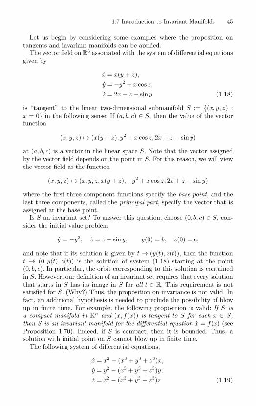
1.7 Introduction to Invariant Manifolds 45
Let us begin by considering some examples where the proposition ontangents and invariant manifolds can be applied.
The vector field on R3 associated with the system of differential equations
given by
x = x(y + z),y = −y2 + x cos z,
z = 2x + z − sin y (1.18)
is “tangent” to the linear two-dimensional submanifold S := (x, y, z) :x = 0 in the following sense: If (a, b, c) ∈ S, then the value of the vectorfunction
(x, y, z) → (x(y + z), y2 + x cos z, 2x + z − sin y)
at (a, b, c) is a vector in the linear space S. Note that the vector assignedby the vector field depends on the point in S. For this reason, we will viewthe vector field as the function
(x, y, z) → (x, y, z, x(y + z),−y2 + x cos z, 2x + z − sin y)
where the first three component functions specify the base point, and thelast three components, called the principal part, specify the vector that isassigned at the base point.
Is S an invariant set? To answer this question, choose (0, b, c) ∈ S, con-sider the initial value problem
y = −y2, z = z − sin y, y(0) = b, z(0) = c,
and note that if its solution is given by t → (y(t), z(t)), then the functiont → (0, y(t), z(t)) is the solution of system (1.18) starting at the point(0, b, c). In particular, the orbit corresponding to this solution is containedin S. However, our definition of an invariant set requires that every solutionthat starts in S has its image in S for all t ∈ R. This requirement is notsatisfied for S. (Why?) Thus, the proposition on invariance is not valid. Infact, an additional hypothesis is needed to preclude the possibility of blowup in finite time. For example, the following proposition is valid: If S isa compact manifold in R
n and (x, f(x)) is tangent to S for each x ∈ S,then S is an invariant manifold for the differential equation x = f(x) (seeProposition 1.70). Indeed, if S is compact, then it is bounded. Thus, asolution with initial point on S cannot blow up in finite time.
The following system of differential equations,
x = x2 − (x3 + y3 + z3)x,
y = y2 − (x3 + y3 + z3)y,
z = z2 − (x3 + y3 + z3)z (1.19)
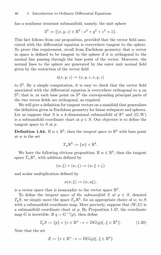
46 1. Introduction to Ordinary Differential Equations
has a nonlinear invariant submanifold; namely, the unit sphere
S2 := (x, y, z) ∈ R
3 : x2 + y2 + z2 = 1.
This fact follows from our proposition, provided that the vector field asso-ciated with the differential equation is everywhere tangent to the sphere.To prove this requirement, recall from Euclidean geometry that a vectorin space is defined to be tangent to the sphere if it is orthogonal to thenormal line passing through the base point of the vector. Moreover, thenormal lines to the sphere are generated by the outer unit normal fieldgiven by the restriction of the vector field
η(x, y, z) := (x, y, z, x, y, z)
to S2. By a simple computation, it is easy to check that the vector field
associated with the differential equation is everywhere orthogonal to η onS
2; that is, at each base point on S2 the corresponding principal parts of
the two vector fields are orthogonal, as required.We will give a definition for tangent vectors on a manifold that generalizes
the definition given in Euclidean geometry for linear subspaces and spheres.Let us suppose that S is a k-dimensional submanifold of R
n and (G, W )is a submanifold coordinate chart at p ∈ S. Our objective is to define thetangent space to S at p.
Definition 1.64. If w ∈ Rk, then the tangent space to R
k with base pointat w is the set
TwRk := w × R
k.
We have the following obvious proposition: If w ∈ Rk, then the tangent
space TwRk, with addition defined by
(w, ξ) + (w, ζ) := (w, ξ + ζ)
and scalar multiplication defined by
a(w, ξ) := (w, aξ),
is a vector space that is isomorphic to the vector space Rk.
To define the tangent space of the submanifold S at p ∈ S, denotedTpS, we simply move the space TwR
k, for an appropriate choice of w, to Swith a submanifold coordinate map. More precisely, suppose that (W, G) isa submanifold coordinate chart at p. By Proposition 1.47, the coordinatemap G is invertible. If q = G−1(p), then define
TpS := p × v ∈ Rn : v = DG(q)ξ, ξ ∈ R
k. (1.20)
Note that the set
S := v ∈ Rn : v = DG(q)ξ, ξ ∈ R
k
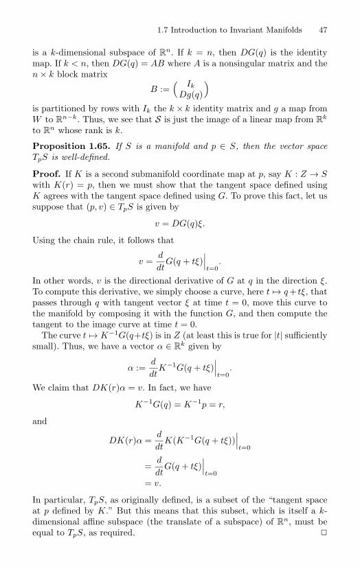
1.7 Introduction to Invariant Manifolds 47
is a k-dimensional subspace of Rn. If k = n, then DG(q) is the identity
map. If k < n, then DG(q) = AB where A is a nonsingular matrix and then × k block matrix
B :=( Ik
Dg(q)
)is partitioned by rows with Ik the k × k identity matrix and g a map fromW to R
n−k. Thus, we see that S is just the image of a linear map from Rk
to Rn whose rank is k.
Proposition 1.65. If S is a manifold and p ∈ S, then the vector spaceTpS is well-defined.
Proof. If K is a second submanifold coordinate map at p, say K : Z → Swith K(r) = p, then we must show that the tangent space defined usingK agrees with the tangent space defined using G. To prove this fact, let ussuppose that (p, v) ∈ TpS is given by
v = DG(q)ξ.
Using the chain rule, it follows that
v =d
dtG(q + tξ)
∣∣∣t=0
.
In other words, v is the directional derivative of G at q in the direction ξ.To compute this derivative, we simply choose a curve, here t → q + tξ, thatpasses through q with tangent vector ξ at time t = 0, move this curve tothe manifold by composing it with the function G, and then compute thetangent to the image curve at time t = 0.
The curve t → K−1G(q+tξ) is in Z (at least this is true for |t| sufficientlysmall). Thus, we have a vector α ∈ R
k given by
α :=d
dtK−1G(q + tξ)
∣∣∣t=0
.
We claim that DK(r)α = v. In fact, we have
K−1G(q) = K−1p = r,
and
DK(r)α =d
dtK(K−1G(q + tξ))
∣∣∣t=0
=d
dtG(q + tξ)
∣∣∣t=0
= v.
In particular, TpS, as originally defined, is a subset of the “tangent spaceat p defined by K.” But this means that this subset, which is itself a k-dimensional affine subspace (the translate of a subspace) of R
n, must beequal to TpS, as required.

48 1. Introduction to Ordinary Differential Equations
Exercise 1.66. Prove: If p ∈ S2, then the tangent space TpS
2, as in Defini-tion 1.20, is equal to
p × v ∈ R3 : 〈p, v〉 = 0.
Definition 1.67. The tangent bundle TS of a manifold S is the union ofits tangent spaces; that is, TS :=
⋃p∈S TpS. Also, for each p ∈ S, the
vector space TpS is called the fiber of the tangent bundle over the basepoint p.
Definition 1.68. Suppose that S1 and S2 are manifolds, and F : S1 → S2is a smooth function. The derivative, also called the tangent map, of F isthe function F∗ : TS1 → TS2 defined as follows: For each (p, v) ∈ TpS1, let(W1, G1) be a submanifold chart at p in S1, (W2, G2) a submanifold chart atF (p) in S2, (G−1
1 (p), ξ) the vector in TG−11 (p)W1 such that DG1(G−1
1 (p))ξ =v, and (G−1
2 (F (p)), ζ) the vector in TG−12 (F (p))W2 such that
ζ = D(G−12 F G1)(G−1
1 (p))ξ.
The tangent vector F∗(p, v) in TF (p)S2 is defined by
F∗(p, v) =(F (p), DG2(G−1
2 (F (p))ζ).
Definition 1.68 certainly seems to be rather complex. However, it is alsovery natural. We simply use the local representatives of the function F andthe definition of the tangent bundle to define the derivative F∗ as the mapwith two component functions. The first component is F (to ensure thatbase points map to base points) and the second component is defined bythe derivative of a local representative of F at each base point.
The following proposition is obvious from the definitions.
Proposition 1.69. The tangent map is well-defined and it is linear oneach fiber of the tangent bundle.
The derivative, or tangent map, of a function defined on a manifold hasa geometric interpretation that is the key to understanding its applicationsin the study of differential equations. We have already discussed this inter-pretation several times for various special cases. However, because it is soimportant, let us consider the geometric interpretation of the derivative inthe context of the notation introduced in Definition 1.68. If t → γ(t) is acurve—a smooth function defined on an open set of R—with image in thesubmanifold S1 ⊆ R
m such that γ(0) = p, and if
v = γ(0) =d
dtγ(t)
∣∣∣t=0
,
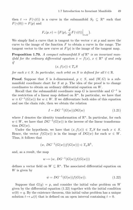
1.7 Introduction to Invariant Manifolds 49
then t → F (γ(t)) is a curve in the submanifold S2 ⊆ Rn such that
F (γ(0)) = F (p) and
F∗(p, v) =(F (p),
d
dtF (γ(t))
∣∣∣t=0
).
We simply find a curve that is tangent to the vector v at p and move thecurve to the image of the function F to obtain a curve in the range. Thetangent vector to the new curve at F (p) is the image of the tangent map.
Proposition 1.70. A compact submanifold S of Rn is an invariant man-
ifold for the ordinary differential equation x = f(x), x ∈ Rn if and only
if(x, f(x)) ∈ TxS
for each x ∈ S. In particular, each orbit on S is defined for all t ∈ R.
Proof. Suppose that S is k-dimensional, p ∈ S, and (W, G) is a sub-manifold coordinate chart for S at p. The idea of the proof is to changecoordinates to obtain an ordinary differential equation on W .
Recall that the submanifold coordinate map G is invertible and G−1 isthe restriction of a linear map defined on R
n. In particular, we have thatw ≡ G−1(G(w)) for w ∈ W . If we differentiate both sides of this equationand use the chain rule, then we obtain the relation
I = DG−1(G(w))DG(w) (1.21)
where I denotes the identity transformation of Rn. In particular, for each
w ∈ W , we have that DG−1(G(w)) is the inverse of the linear transforma-tion DG(w).
Under the hypothesis, we have that (x, f(x)) ∈ TxS for each x ∈ S.Hence, the vector f(G(w)) is in the image of DG(w) for each w ∈ W .Thus, it follows that
(w, DG−1(G(w))f(G(w))) ∈ TwRk,
and, as a result, the map
w → (w, DG−1(G(w))f(G(w)))
defines a vector field on W ⊆ Rn. The associated differential equation on
W is given by
w = DG−1(G(w))f(G(w)). (1.22)
Suppose that G(q) = p, and consider the initial value problem on Wgiven by the differential equation (1.22) together with the initial conditionw(0) = q. By the existence theorem, this initial value problem has a uniquesolution t → ω(t) that is defined on an open interval containing t = 0.
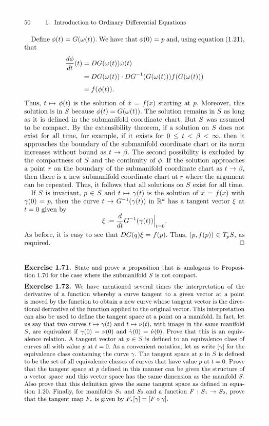
50 1. Introduction to Ordinary Differential Equations
Define φ(t) = G(ω(t)). We have that φ(0) = p and, using equation (1.21),that
dφ
dt(t) = DG(ω(t))ω(t)
= DG(ω(t)) · DG−1(G(ω(t)))f(G(ω(t)))
= f(φ(t)).
Thus, t → φ(t) is the solution of x = f(x) starting at p. Moreover, thissolution is in S because φ(t) = G(ω(t)). The solution remains in S as longas it is defined in the submanifold coordinate chart. But S was assumedto be compact. By the extensibility theorem, if a solution on S does notexist for all time, for example, if it exists for 0 ≤ t < β < ∞, then itapproaches the boundary of the submanifold coordinate chart or its normincreases without bound as t → β. The second possibility is excluded bythe compactness of S and the continuity of φ. If the solution approachesa point r on the boundary of the submanifold coordinate chart as t → β,then there is a new submanifold coordinate chart at r where the argumentcan be repeated. Thus, it follows that all solutions on S exist for all time.
If S is invariant, p ∈ S and t → γ(t) is the solution of x = f(x) withγ(0) = p, then the curve t → G−1(γ(t)) in R
k has a tangent vector ξ att = 0 given by
ξ :=d
dtG−1(γ(t))
∣∣∣t=0
.
As before, it is easy to see that DG(q)ξ = f(p). Thus, (p, f(p)) ∈ TpS, asrequired.
Exercise 1.71. State and prove a proposition that is analogous to Proposi-tion 1.70 for the case where the submanifold S is not compact.
Exercise 1.72. We have mentioned several times the interpretation of thederivative of a function whereby a curve tangent to a given vector at a pointis moved by the function to obtain a new curve whose tangent vector is the direc-tional derivative of the function applied to the original vector. This interpretationcan also be used to define the tangent space at a point on a manifold. In fact, letus say that two curves t → γ(t) and t → ν(t), with image in the same manifoldS, are equivalent if γ(0) = ν(0) and γ(0) = ν(0). Prove that this is an equiv-alence relation. A tangent vector at p ∈ S is defined to an equivalence class ofcurves all with value p at t = 0. As a convenient notation, let us write [γ] for theequivalence class containing the curve γ. The tangent space at p in S is definedto be the set of all equivalence classes of curves that have value p at t = 0. Provethat the tangent space at p defined in this manner can be given the structure ofa vector space and this vector space has the same dimension as the manifold S.Also prove that this definition gives the same tangent space as defined in equa-tion 1.20. Finally, for manifolds S1 and S2 and a function F : S1 → S2, provethat the tangent map F∗ is given by F∗[γ] = [F γ].
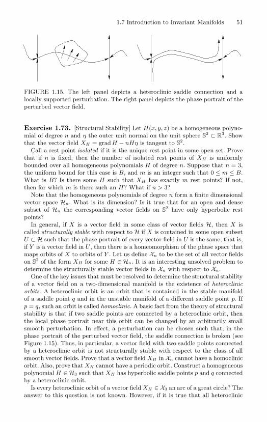
1.7 Introduction to Invariant Manifolds 51
FIGURE 1.15. The left panel depicts a heteroclinic saddle connection and alocally supported perturbation. The right panel depicts the phase portrait of theperturbed vector field.
Exercise 1.73. [Structural Stability] Let H(x, y, z) be a homogeneous polyno-mial of degree n and η the outer unit normal on the unit sphere S
2 ⊂ R3. Show
that the vector field XH = grad H − nHη is tangent to S2.
Call a rest point isolated if it is the unique rest point in some open set. Provethat if n is fixed, then the number of isolated rest points of XH is uniformlybounded over all homogeneous polynomials H of degree n. Suppose that n = 3,the uniform bound for this case is B, and m is an integer such that 0 ≤ m ≤ B.What is B? Is there some H such that XH has exactly m rest points? If not,then for which m is there such an H? What if n > 3?
Note that the homogeneous polynomials of degree n form a finite dimensionalvector space Hn. What is its dimension? Is it true that for an open and densesubset of Hn the corresponding vector fields on S
2 have only hyperbolic restpoints?
In general, if X is a vector field in some class of vector fields H, then X iscalled structurally stable with respect to H if X is contained in some open subsetU ⊂ H such that the phase portrait of every vector field in U is the same; that is,if Y is a vector field in U , then there is a homeomorphism of the phase space thatmaps orbits of X to orbits of Y . Let us define Xn to be the set of all vector fieldson S
2 of the form XH for some H ∈ Hn. It is an interesting unsolved problem todetermine the structurally stable vector fields in Xn with respect to Xn.
One of the key issues that must be resolved to determine the structural stabilityof a vector field on a two-dimensional manifold is the existence of heteroclinicorbits. A heteroclinic orbit is an orbit that is contained in the stable manifoldof a saddle point q and in the unstable manifold of a different saddle point p. Ifp = q, such an orbit is called homoclinic. A basic fact from the theory of structuralstability is that if two saddle points are connected by a heteroclinic orbit, thenthe local phase portrait near this orbit can be changed by an arbitrarily smallsmooth perturbation. In effect, a perturbation can be chosen such that, in thephase portrait of the perturbed vector field, the saddle connection is broken (seeFigure 1.15). Thus, in particular, a vector field with two saddle points connectedby a heteroclinic orbit is not structurally stable with respect to the class of allsmooth vector fields. Prove that a vector field XH in Xn cannot have a homoclinicorbit. Also, prove that XH cannot have a periodic orbit. Construct a homogeneouspolynomial H ∈ H3 such that XH has hyperbolic saddle points p and q connectedby a heteroclinic orbit.
Is every heteroclinic orbit of a vector field XH ∈ X3 an arc of a great circle? Theanswer to this question is not known. However, if it is true that all heteroclinic
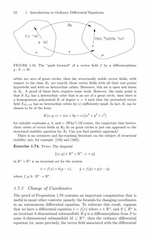
52 1. Introduction to Ordinary Differential Equations
S
Dggyfgygy
y
fgy
Dg
g
M
FIGURE 1.16. The “push forward” of a vector field f by a diffeomorphismg : S → M .
orbits are arcs of great circles, then the structurally stable vector fields, withrespect to the class X3, are exactly those vector fields with all their rest pointshyperbolic and with no heteroclinic orbits. Moreover, this set is open and densein Xn. A proof of these facts requires some work. However, the main point isthat if XH has a heteroclinic orbit that is an arc of a great circle, then there isa homogeneous polynomial K of degree n = 3 such that the perturbed vectorfield XH+εK has no heteroclinic orbits for |ε| sufficiently small. In fact, K can bechosen to be of the form
K(x, y, z) = (ax + by + cz)(x2 + y2 + z2)
for suitable constants a, b, and c. (Why?) Of course, the conjecture that hetero-clinic orbits of vector fields in H3 lie on great circles is just one approach to thestructural stability question for X3. Can you find another approach?
There is an extensive and far-reaching literature on the subject of structuralstability (see, for example, [150] and [160]).
Exercise 1.74. Prove: The diagonal
(x, y) ∈ Rn × R
n : x = y
in Rn × R
n is an invariant set for the system
x = f(x) + h(y − x), y = f(y) + g(x − y)
where f, g, h : Rn → R
n.
1.7.3 Change of CoordinatesThe proof of Proposition 1.70 contains an important computation that isuseful in many other contexts; namely, the formula for changing coordinatesin an autonomous differential equation. To reiterate this result, supposethat we have a differential equation x = f(x) where x ∈ R
n, and S ⊆ Rn is
an invariant k-dimensional submanifold. If g is a diffeomorphism from S tosome k-dimensional submanifold M ⊆ R
m, then the ordinary differentialequation (or, more precisely, the vector field associated with the differential
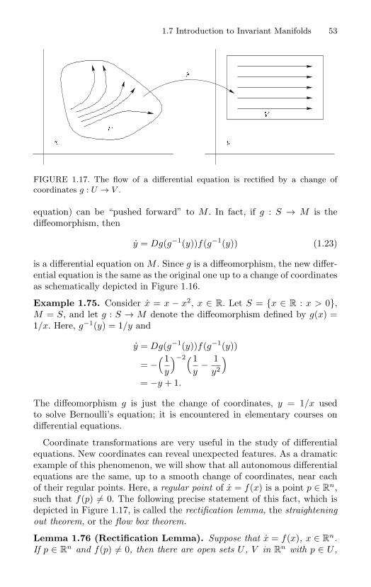
1.7 Introduction to Invariant Manifolds 53
g
U
x y
V
FIGURE 1.17. The flow of a differential equation is rectified by a change ofcoordinates g : U → V .
equation) can be “pushed forward” to M . In fact, if g : S → M is thediffeomorphism, then
y = Dg(g−1(y))f(g−1(y)) (1.23)
is a differential equation on M . Since g is a diffeomorphism, the new differ-ential equation is the same as the original one up to a change of coordinatesas schematically depicted in Figure 1.16.
Example 1.75. Consider x = x − x2, x ∈ R. Let S = x ∈ R : x > 0,M = S, and let g : S → M denote the diffeomorphism defined by g(x) =1/x. Here, g−1(y) = 1/y and
y = Dg(g−1(y))f(g−1(y))
= −(1
y
)−2(1y
− 1y2
)= −y + 1.
The diffeomorphism g is just the change of coordinates, y = 1/x usedto solve Bernoulli’s equation; it is encountered in elementary courses ondifferential equations.
Coordinate transformations are very useful in the study of differentialequations. New coordinates can reveal unexpected features. As a dramaticexample of this phenomenon, we will show that all autonomous differentialequations are the same, up to a smooth change of coordinates, near eachof their regular points. Here, a regular point of x = f(x) is a point p ∈ R
n,such that f(p) = 0. The following precise statement of this fact, which isdepicted in Figure 1.17, is called the rectification lemma, the straighteningout theorem, or the flow box theorem.
Lemma 1.76 (Rectification Lemma). Suppose that x = f(x), x ∈ Rn.
If p ∈ Rn and f(p) = 0, then there are open sets U , V in R
n with p ∈ U ,
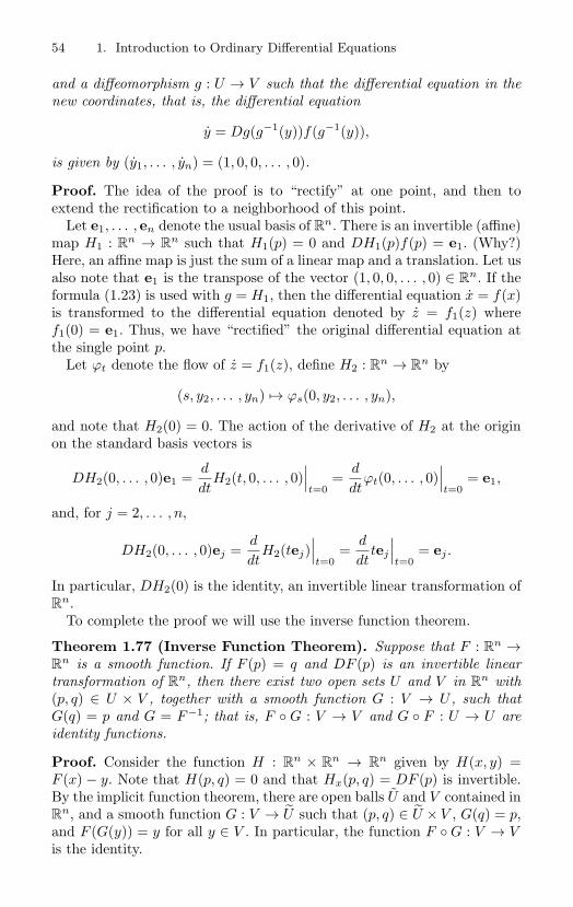
54 1. Introduction to Ordinary Differential Equations
and a diffeomorphism g : U → V such that the differential equation in thenew coordinates, that is, the differential equation
y = Dg(g−1(y))f(g−1(y)),
is given by (y1, . . . , yn) = (1, 0, 0, . . . , 0).
Proof. The idea of the proof is to “rectify” at one point, and then toextend the rectification to a neighborhood of this point.
Let e1, . . . , en denote the usual basis of Rn. There is an invertible (affine)
map H1 : Rn → R
n such that H1(p) = 0 and DH1(p)f(p) = e1. (Why?)Here, an affine map is just the sum of a linear map and a translation. Let usalso note that e1 is the transpose of the vector (1, 0, 0, . . . , 0) ∈ R
n. If theformula (1.23) is used with g = H1, then the differential equation x = f(x)is transformed to the differential equation denoted by z = f1(z) wheref1(0) = e1. Thus, we have “rectified” the original differential equation atthe single point p.
Let ϕt denote the flow of z = f1(z), define H2 : Rn → R
n by
(s, y2, . . . , yn) → ϕs(0, y2, . . . , yn),
and note that H2(0) = 0. The action of the derivative of H2 at the originon the standard basis vectors is
DH2(0, . . . , 0)e1 =d
dtH2(t, 0, . . . , 0)
∣∣∣t=0
=d
dtϕt(0, . . . , 0)
∣∣∣t=0
= e1,
and, for j = 2, . . . , n,
DH2(0, . . . , 0)ej =d
dtH2(tej)
∣∣∣t=0
=d
dttej
∣∣∣t=0
= ej .
In particular, DH2(0) is the identity, an invertible linear transformation ofR
n.To complete the proof we will use the inverse function theorem.
Theorem 1.77 (Inverse Function Theorem). Suppose that F : Rn →
Rn is a smooth function. If F (p) = q and DF (p) is an invertible linear
transformation of Rn, then there exist two open sets U and V in R
n with(p, q) ∈ U × V , together with a smooth function G : V → U , such thatG(q) = p and G = F−1; that is, F G : V → V and G F : U → U areidentity functions.
Proof. Consider the function H : Rn × R
n → Rn given by H(x, y) =
F (x) − y. Note that H(p, q) = 0 and that Hx(p, q) = DF (p) is invertible.By the implicit function theorem, there are open balls U and V contained inR
n, and a smooth function G : V → U such that (p, q) ∈ U × V , G(q) = p,and F (G(y)) = y for all y ∈ V . In particular, the function F G : V → Vis the identity.
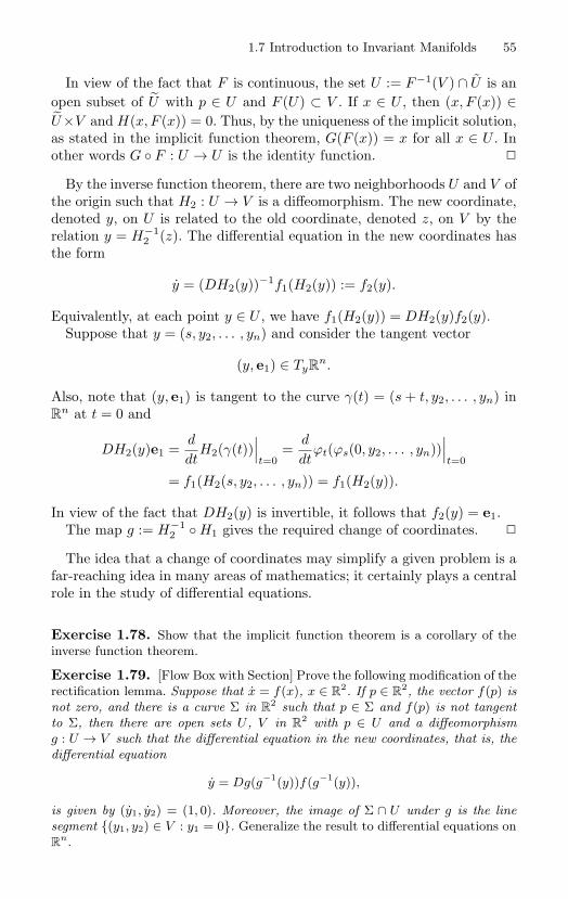
1.7 Introduction to Invariant Manifolds 55
In view of the fact that F is continuous, the set U := F−1(V ) ∩ U is anopen subset of U with p ∈ U and F (U) ⊂ V . If x ∈ U , then (x, F (x)) ∈U×V and H(x, F (x)) = 0. Thus, by the uniqueness of the implicit solution,as stated in the implicit function theorem, G(F (x)) = x for all x ∈ U . Inother words G F : U → U is the identity function.
By the inverse function theorem, there are two neighborhoods U and V ofthe origin such that H2 : U → V is a diffeomorphism. The new coordinate,denoted y, on U is related to the old coordinate, denoted z, on V by therelation y = H−1
2 (z). The differential equation in the new coordinates hasthe form
y = (DH2(y))−1f1(H2(y)) := f2(y).
Equivalently, at each point y ∈ U , we have f1(H2(y)) = DH2(y)f2(y).Suppose that y = (s, y2, . . . , yn) and consider the tangent vector
(y, e1) ∈ TyRn.
Also, note that (y, e1) is tangent to the curve γ(t) = (s + t, y2, . . . , yn) inR
n at t = 0 and
DH2(y)e1 =d
dtH2(γ(t))
∣∣∣t=0
=d
dtϕt(ϕs(0, y2, . . . , yn))
∣∣∣t=0
= f1(H2(s, y2, . . . , yn)) = f1(H2(y)).
In view of the fact that DH2(y) is invertible, it follows that f2(y) = e1.The map g := H−1
2 H1 gives the required change of coordinates.
The idea that a change of coordinates may simplify a given problem is afar-reaching idea in many areas of mathematics; it certainly plays a centralrole in the study of differential equations.
Exercise 1.78. Show that the implicit function theorem is a corollary of theinverse function theorem.
Exercise 1.79. [Flow Box with Section] Prove the following modification of therectification lemma. Suppose that x = f(x), x ∈ R
2. If p ∈ R2, the vector f(p) is
not zero, and there is a curve Σ in R2 such that p ∈ Σ and f(p) is not tangent
to Σ, then there are open sets U , V in R2 with p ∈ U and a diffeomorphism
g : U → V such that the differential equation in the new coordinates, that is, thedifferential equation
y = Dg(g−1(y))f(g−1(y)),
is given by (y1, y2) = (1, 0). Moreover, the image of Σ ∩ U under g is the linesegment (y1, y2) ∈ V : y1 = 0. Generalize the result to differential equations onR
n.
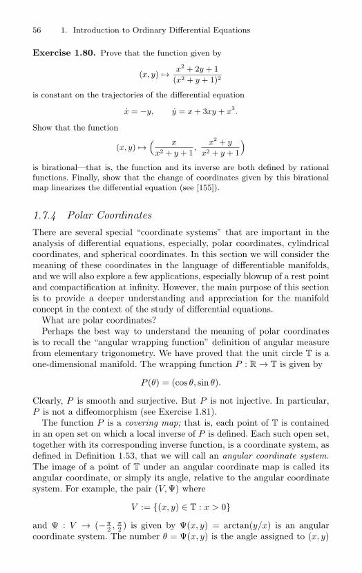
56 1. Introduction to Ordinary Differential Equations
Exercise 1.80. Prove that the function given by
(x, y) → x2 + 2y + 1(x2 + y + 1)2
is constant on the trajectories of the differential equation
x = −y, y = x + 3xy + x3.
Show that the function
(x, y) →( x
x2 + y + 1,
x2 + y
x2 + y + 1
)
is birational—that is, the function and its inverse are both defined by rationalfunctions. Finally, show that the change of coordinates given by this birationalmap linearizes the differential equation (see [155]).
1.7.4 Polar CoordinatesThere are several special “coordinate systems” that are important in theanalysis of differential equations, especially, polar coordinates, cylindricalcoordinates, and spherical coordinates. In this section we will consider themeaning of these coordinates in the language of differentiable manifolds,and we will also explore a few applications, especially blowup of a rest pointand compactification at infinity. However, the main purpose of this sectionis to provide a deeper understanding and appreciation for the manifoldconcept in the context of the study of differential equations.
What are polar coordinates?Perhaps the best way to understand the meaning of polar coordinates
is to recall the “angular wrapping function” definition of angular measurefrom elementary trigonometry. We have proved that the unit circle T is aone-dimensional manifold. The wrapping function P : R → T is given by
P (θ) = (cos θ, sin θ).
Clearly, P is smooth and surjective. But P is not injective. In particular,P is not a diffeomorphism (see Exercise 1.81).
The function P is a covering map; that is, each point of T is containedin an open set on which a local inverse of P is defined. Each such open set,together with its corresponding inverse function, is a coordinate system, asdefined in Definition 1.53, that we will call an angular coordinate system.The image of a point of T under an angular coordinate map is called itsangular coordinate, or simply its angle, relative to the angular coordinatesystem. For example, the pair (V, Ψ) where
V := (x, y) ∈ T : x > 0
and Ψ : V → (−π2 , π
2 ) is given by Ψ(x, y) = arctan(y/x) is an angularcoordinate system. The number θ = Ψ(x, y) is the angle assigned to (x, y)
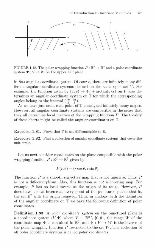
1.7 Introduction to Invariant Manifolds 57
W
V
x
P
r
y
FIGURE 1.18. The polar wrapping function P : R2 → R
2 and a polar coordinatesystem Ψ : V → W on the upper half plane.
in this angular coordinate system. Of course, there are infinitely many dif-ferent angular coordinate systems defined on the same open set V . Forexample, the function given by (x, y) → 4π + arctan(y/x) on V also de-termines an angular coordinate system on T for which the correspondingangles belong to the interval ( 7π
2 , 9π2 ).
As we have just seen, each point of T is assigned infinitely many angles.However, all angular coordinate systems are compatible in the sense thatthey all determine local inverses of the wrapping function P . The totalityof these charts might be called the angular coordinates on T.
Exercise 1.81. Prove that T is not diffeomorphic to R.
Exercise 1.82. Find a collection of angular coordinate systems that cover theunit circle.
Let us next consider coordinates on the plane compatible with the polarwrapping function P : R
2 → R2 given by
P (r, θ) = (r cos θ, r sin θ).
The function P is a smooth surjective map that is not injective. Thus, Pis not a diffeomorphism. Also, this function is not a covering map. Forexample, P has no local inverse at the origin of its range. However, Pdoes have a local inverse at every point of the punctured plane; that is,the set R
2 with the origin removed. Thus, in analogy with the definitionof the angular coordinate on T we have the following definition of polarcoordinates.
Definition 1.83. A polar coordinate system on the punctured plane isa coordinate system (V, Ψ) where V ⊂ R
2 \ 0, 0, the range W of thecoordinate map Ψ is contained in R
2, and Ψ : V → W is the inverse ofthe polar wrapping function P restricted to the set W . The collection ofall polar coordinate systems is called polar coordinates.
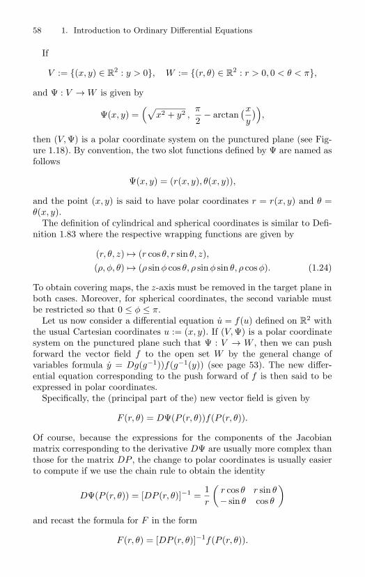
58 1. Introduction to Ordinary Differential Equations
If
V := (x, y) ∈ R2 : y > 0, W := (r, θ) ∈ R
2 : r > 0, 0 < θ < π,
and Ψ : V → W is given by
Ψ(x, y) =(√
x2 + y2 ,π
2− arctan
(x
y
)),
then (V, Ψ) is a polar coordinate system on the punctured plane (see Fig-ure 1.18). By convention, the two slot functions defined by Ψ are named asfollows
Ψ(x, y) = (r(x, y), θ(x, y)),
and the point (x, y) is said to have polar coordinates r = r(x, y) and θ =θ(x, y).
The definition of cylindrical and spherical coordinates is similar to Defi-nition 1.83 where the respective wrapping functions are given by
(r, θ, z) → (r cos θ, r sin θ, z),(ρ, φ, θ) → (ρ sin φ cos θ, ρ sin φ sin θ, ρ cos φ). (1.24)
To obtain covering maps, the z-axis must be removed in the target plane inboth cases. Moreover, for spherical coordinates, the second variable mustbe restricted so that 0 ≤ φ ≤ π.
Let us now consider a differential equation u = f(u) defined on R2 with
the usual Cartesian coordinates u := (x, y). If (V, Ψ) is a polar coordinatesystem on the punctured plane such that Ψ : V → W , then we can pushforward the vector field f to the open set W by the general change ofvariables formula y = Dg(g−1))f(g−1(y)) (see page 53). The new differ-ential equation corresponding to the push forward of f is then said to beexpressed in polar coordinates.
Specifically, the (principal part of the) new vector field is given by
F (r, θ) = DΨ(P (r, θ))f(P (r, θ)).
Of course, because the expressions for the components of the Jacobianmatrix corresponding to the derivative DΨ are usually more complex thanthose for the matrix DP , the change to polar coordinates is usually easierto compute if we use the chain rule to obtain the identity
DΨ(P (r, θ)) = [DP (r, θ)]−1 =1r
(r cos θ r sin θ− sin θ cos θ
)and recast the formula for F in the form
F (r, θ) = [DP (r, θ)]−1f(P (r, θ)).
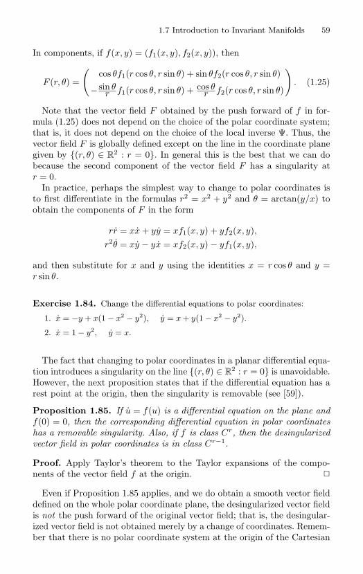
1.7 Introduction to Invariant Manifolds 59
In components, if f(x, y) = (f1(x, y), f2(x, y)), then
F (r, θ) =
(cos θf1(r cos θ, r sin θ) + sin θf2(r cos θ, r sin θ)
− sin θr f1(r cos θ, r sin θ) + cos θ
r f2(r cos θ, r sin θ)
). (1.25)
Note that the vector field F obtained by the push forward of f in for-mula (1.25) does not depend on the choice of the polar coordinate system;that is, it does not depend on the choice of the local inverse Ψ. Thus, thevector field F is globally defined except on the line in the coordinate planegiven by (r, θ) ∈ R
2 : r = 0. In general this is the best that we can dobecause the second component of the vector field F has a singularity atr = 0.
In practice, perhaps the simplest way to change to polar coordinates isto first differentiate in the formulas r2 = x2 + y2 and θ = arctan(y/x) toobtain the components of F in the form
rr = xx + yy = xf1(x, y) + yf2(x, y),r2θ = xy − yx = xf2(x, y) − yf1(x, y),
and then substitute for x and y using the identities x = r cos θ and y =r sin θ.
Exercise 1.84. Change the differential equations to polar coordinates:
1. x = −y + x(1 − x2 − y2), y = x + y(1 − x2 − y2).
2. x = 1 − y2, y = x.
The fact that changing to polar coordinates in a planar differential equa-tion introduces a singularity on the line (r, θ) ∈ R
2 : r = 0 is unavoidable.However, the next proposition states that if the differential equation has arest point at the origin, then the singularity is removable (see [59]).
Proposition 1.85. If u = f(u) is a differential equation on the plane andf(0) = 0, then the corresponding differential equation in polar coordinateshas a removable singularity. Also, if f is class Cr, then the desingularizedvector field in polar coordinates is in class Cr−1.
Proof. Apply Taylor’s theorem to the Taylor expansions of the compo-nents of the vector field f at the origin.
Even if Proposition 1.85 applies, and we do obtain a smooth vector fielddefined on the whole polar coordinate plane, the desingularized vector fieldis not the push forward of the original vector field; that is, the desingular-ized vector field is not obtained merely by a change of coordinates. Remem-ber that there is no polar coordinate system at the origin of the Cartesian
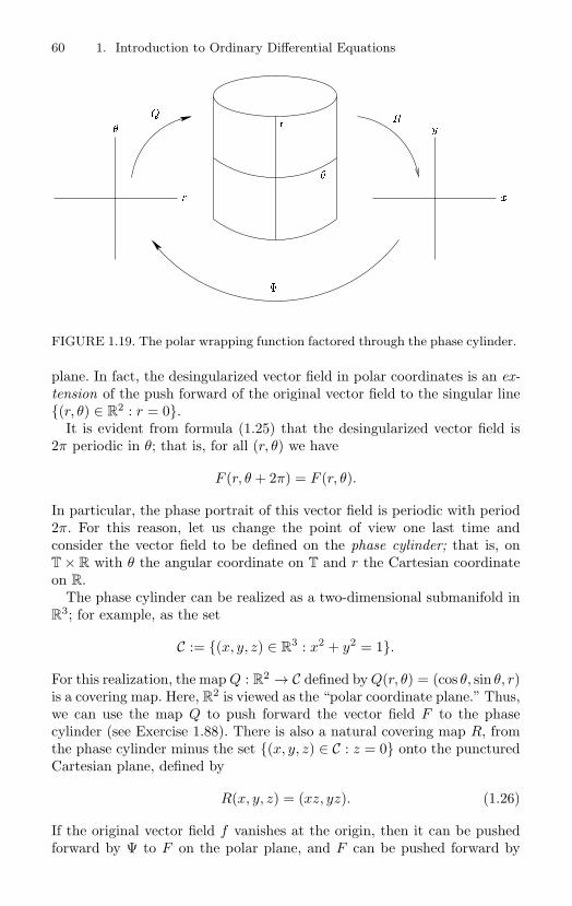
60 1. Introduction to Ordinary Differential Equations
r
x
yR
Q
r
FIGURE 1.19. The polar wrapping function factored through the phase cylinder.
plane. In fact, the desingularized vector field in polar coordinates is an ex-tension of the push forward of the original vector field to the singular line(r, θ) ∈ R
2 : r = 0.It is evident from formula (1.25) that the desingularized vector field is
2π periodic in θ; that is, for all (r, θ) we have
F (r, θ + 2π) = F (r, θ).
In particular, the phase portrait of this vector field is periodic with period2π. For this reason, let us change the point of view one last time andconsider the vector field to be defined on the phase cylinder; that is, onT × R with θ the angular coordinate on T and r the Cartesian coordinateon R.
The phase cylinder can be realized as a two-dimensional submanifold inR
3; for example, as the set
C := (x, y, z) ∈ R3 : x2 + y2 = 1.
For this realization, the map Q : R2 → C defined by Q(r, θ) = (cos θ, sin θ, r)
is a covering map. Here, R2 is viewed as the “polar coordinate plane.” Thus,
we can use the map Q to push forward the vector field F to the phasecylinder (see Exercise 1.88). There is also a natural covering map R, fromthe phase cylinder minus the set (x, y, z) ∈ C : z = 0 onto the puncturedCartesian plane, defined by
R(x, y, z) = (xz, yz). (1.26)
If the original vector field f vanishes at the origin, then it can be pushedforward by Ψ to F on the polar plane, and F can be pushed forward by
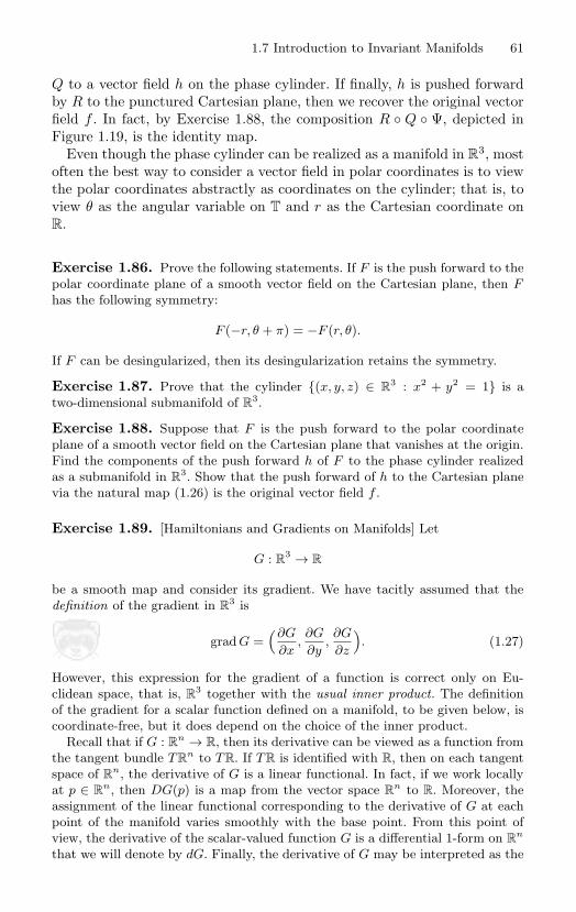
1.7 Introduction to Invariant Manifolds 61
Q to a vector field h on the phase cylinder. If finally, h is pushed forwardby R to the punctured Cartesian plane, then we recover the original vectorfield f . In fact, by Exercise 1.88, the composition R Q Ψ, depicted inFigure 1.19, is the identity map.
Even though the phase cylinder can be realized as a manifold in R3, most
often the best way to consider a vector field in polar coordinates is to viewthe polar coordinates abstractly as coordinates on the cylinder; that is, toview θ as the angular variable on T and r as the Cartesian coordinate onR.
Exercise 1.86. Prove the following statements. If F is the push forward to thepolar coordinate plane of a smooth vector field on the Cartesian plane, then Fhas the following symmetry:
F (−r, θ + π) = −F (r, θ).
If F can be desingularized, then its desingularization retains the symmetry.
Exercise 1.87. Prove that the cylinder (x, y, z) ∈ R3 : x2 + y2 = 1 is a
two-dimensional submanifold of R3.
Exercise 1.88. Suppose that F is the push forward to the polar coordinateplane of a smooth vector field on the Cartesian plane that vanishes at the origin.Find the components of the push forward h of F to the phase cylinder realizedas a submanifold in R
3. Show that the push forward of h to the Cartesian planevia the natural map (1.26) is the original vector field f .
Exercise 1.89. [Hamiltonians and Gradients on Manifolds] Let
G : R3 → R
be a smooth map and consider its gradient. We have tacitly assumed that thedefinition of the gradient in R
3 is
grad G =(∂G
∂x,∂G
∂y,∂G
∂z
). (1.27)
However, this expression for the gradient of a function is correct only on Eu-clidean space, that is, R
3 together with the usual inner product. The definitionof the gradient for a scalar function defined on a manifold, to be given below, iscoordinate-free, but it does depend on the choice of the inner product.
Recall that if G : Rn → R, then its derivative can be viewed as a function from
the tangent bundle TRn to TR. If TR is identified with R, then on each tangent
space of Rn, the derivative of G is a linear functional. In fact, if we work locally
at p ∈ Rn, then DG(p) is a map from the vector space R
n to R. Moreover, theassignment of the linear functional corresponding to the derivative of G at eachpoint of the manifold varies smoothly with the base point. From this point ofview, the derivative of the scalar-valued function G is a differential 1-form on R
n
that we will denote by dG. Finally, the derivative of G may be interpreted as the
62 1. Introduction to Ordinary Differential Equations
the differential of G. In this interpretation, if V is a tangent vector at p ∈ Rn
and γ is a curve such that γ(0) = p and γ(0) = V , then
dG(V ) =d
dsG(γ(s))
∣∣∣s=0
.
If G is a scalar function defined on a manifold, then all of our interpretations forthe derivative of G are still viable.
The definition of the gradient requires a new concept: A Riemannian metric ona manifold is a smooth assignment of an inner product in each tangent space ofthe manifold. Of course, the usual inner product assigned in each tangent space ofR
n is a Riemannian metric for Rn. Moreover, the manifold R
n together with thisRiemannian metric is called Euclidean space. Note that the Riemannian metriccan be used to define length. For example, the norm of a vector is the square rootof the inner product of the vector with itself. It follows that the shortest distancebetween two points is a straight line. Thus, the geometry of Euclidean space isEuclidean geometry, as it should be. More generally, if γ is a curve in Euclideanspace connecting two points p and q; that is, γ(0) = p and γ(1) = q, then thelength of the curve
∫ 1
0
√〈γ(t), γ(t)〉 dt,
where the angle brackets denote the usual inner product, is minimized over allsuch curves defined on the unit interval by the curve γ(t) = tq + (1 − t)p thatparametrizes the straight line joining the points. Similarly, suppose that g is aRiemannian metric on a manifold M and p, q ∈ M . Roughly speaking, a curvedefined on the unit interval that joins the points p and q is called a geodesic if itminimizes the integral
∫ 1
0
√gγ(t)(γ(t), γ(t)) dt
where, in general, the symbolism gr(v, w) denotes the inner product of the twovectors (r, v) and (r, w) in TrM . The “Riemannian geometry” on a manifoldwhere geodesics play the role of lines is determined by the choice of a Riemannianmetric.
The gradient of G : M → R with respect to the Riemannian metric g is thevector field, denoted by grad G, such that
dGp(V ) = gp(V, grad G) (1.28)
for each point p ∈ M and every tangent vector V ∈ TpM . The associated gradientsystem on the manifold is the differential equation p = grad G(p).
Prove: The gradient vector field is uniquely defined. Prove: If the Riemannianmetric g on R
3 is the usual inner product at each point of R3, then the invariant
definition (1.28) of gradient agrees with the Euclidean gradient.Consider the upper half plane of R
2 with the Riemannian metric
g(x,y)(V, W ) = y−2〈V, W 〉 (1.29)
where the angle brackets denote the usual inner product. The upper half planewith the metric g is called the Poincare or Lobachevsky plane; its geodesics are
1.7 Introduction to Invariant Manifolds 63
vertical lines and arcs of circles whose centers are on the x-axis. The geometryis non-Euclidean; for example, if p is a point not on such a circle, then thereare infinitely many such circles passing through p that are parallel to (do notintersect) the given circle.
Find the gradient of the function G(x, y) = x2 + y2 with respect to the Rie-mannian metric (1.29) and draw the phase portrait of the corresponding gradientsystem on the upper half plane. Compare this phase portrait with the phase por-trait of the gradient system with respect to the usual metric on the plane.
If S is a submanifold of Rn, then S inherits a Riemannian metric from the
usual inner product on Rn. Suppose that F : R
n → R. What is the relationshipbetween the gradient of F on R
n and the gradient of the function F restricted toS with respect to the inherited Riemannian metric (see Exercise 1.73)?
Hamiltonian systems on manifolds are defined in essentially the same way asgradient systems except that the Riemannian metric is replaced by a symplecticform. In order to properly define and analyze symplectic forms, the calculus ofdifferential forms is required (see [10], [68], and [167]). However, for completeness,a symplectic form on a manifold is a smooth assignment of a bilinear, skew-symmetric, nondegenerate 2-form in each tangent space. A 2-form ω on a vectorspace X is nondegenerate provided that y = 0 is the only element of X such thatω(x, y) = 0 for all x ∈ X. Prove: If a manifold has a symplectic form, then thedimension of the manifold is even.
Suppose that M is a manifold and ω is a symplectic form on M . The Hamilto-nian vector field associated with a smooth scalar function H defined on M is theunique vector field XH such that, for every point p ∈ M and all tangent vectorsV at p, the following identity holds:
dHp(V ) = ωp(XH , V ). (1.30)
Suppose that M := R2n, view R
2n as Rn × R
n so that each tangent vector Von M is decomposed as V = (V1, V2) with V1, V2 ∈ R
n, and define
ω(V, W ) := (V1, V2)(
0 I−I 0
) (W1
W2
).
Show that ω is a symplectic form on M and Hamilton’s equations are producedby the invariant definition (1.30) of the Hamiltonian vector field.
Push forward the Euclidean gradient (1.27) of the function G : R3 → R to the
image of a cylindrical coordinate map, define
G(r, θ, z) = G(r cos θ, r sin θ, z),
and show that the push forward gives the result
grad G =(∂G
∂r,
1r2
∂G∂θ
,∂G∂z
). (1.31)
(In practice, the function G is usually again called G! These two functions arelocal representations of the same function in two different coordinate systems.)Recall the formula for the gradient in cylindrical coordinates from vector analysis;namely,
grad G =∂G∂r
er +1r
∂G∂θ
eθ +∂G∂z
ez. (1.32)
64 1. Introduction to Ordinary Differential Equations
Show that the gradient vector fields (1.31) and (1.32) coincide.Express the usual inner product in cylindrical coordinates, and use the invari-
ant definition of the gradient to determine the gradient in cylindrical coordinates.Repeat the exercise for spherical coordinates.
Exercise 1.90. [Electrostatic Dipole Potential] Suppose that two point chargeswith opposite signs, each with charge q, placed a units apart and located symmet-rically with respect to the origin on the z-axis in space, produce the electrostaticpotential
G0(x, y, z) = kq[(x2 + y2 + (z − a
2)2)−1/2 − (x2 + y2 + (z +
a
2)2)−1/2]
where k > 0 is a constant and q > 0. If we are interested only in the field farfrom the charges, the “far field,” then a is relatively small and therefore the firstnonzero term of the Taylor series of the electrostatic potential with respect to aat a = 0 gives a useful approximation of G0. This approximation, an example ofa “far field approximation,” is called the dipole potential in Physics (see [66, Vol.II, 6-1]). Show that the dipole potential is given by
G(x, y, z) = kqaz(x2 + y2 + z2)−3/2.
By definition, the electric field E produced by the dipole potential associated withthe two charges is E := − grad G. Draw the phase portrait of the differentialequation u = E(u) whose orbits are the “dipole” lines of force. Discuss thestability of all rest points. Hint: Choose a useful coordinate system that reducesthe problem to two dimensions.
Blow Up at a Rest Point
As an application of polar coordinates, let us determine the phase portraitof the differential equation in the Cartesian plane given by
x = x2 − 2xy, y = y2 − 2xy, (1.33)
(see [59]). This system has a unique rest point at the origin that is nothyperbolic. In fact, the system matrix for the linearization at the originvanishes. Thus, linearization provides no information about the phase por-trait of the system near the origin.
Because the polar coordinate representation of a plane vector field isalways singular at the origin, we might expect that the polar coordinaterepresentation of a planar vector field is not particularly useful to determinethe phase portrait near the origin. However, this is not the case. Oftenpolar coordinates are the best way to analyze the vector field near theorigin. The reason is that the desingularized vector field in polar coordinatesis a smooth extension to the singular line represented as the equator ofthe phase cylinder. All points on the equator are collapsed to the singlerest point at the origin in the Cartesian plane. Or, as we say, the equatoris the blowup of the rest point. This extension is valuable because thephase portrait of the vector field near the original rest point corresponds
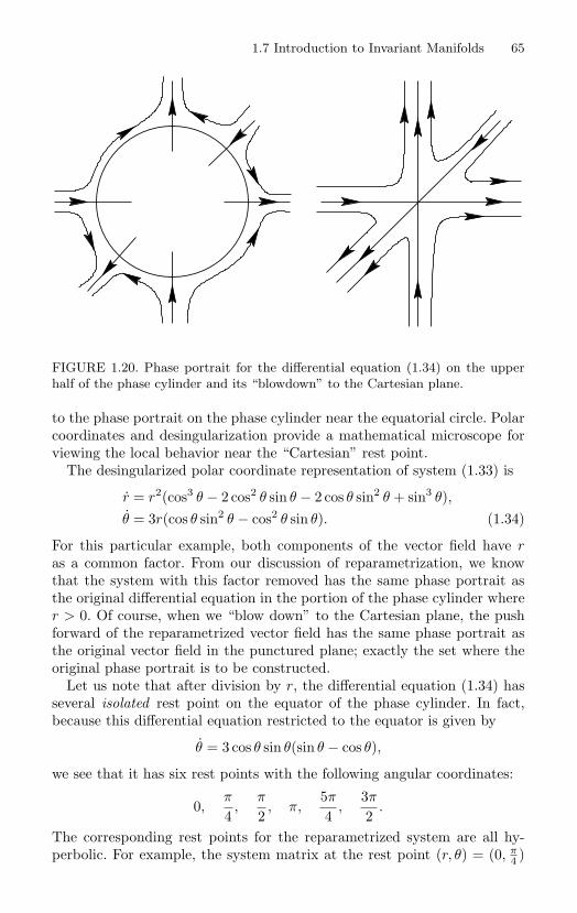
1.7 Introduction to Invariant Manifolds 65
FIGURE 1.20. Phase portrait for the differential equation (1.34) on the upperhalf of the phase cylinder and its “blowdown” to the Cartesian plane.
to the phase portrait on the phase cylinder near the equatorial circle. Polarcoordinates and desingularization provide a mathematical microscope forviewing the local behavior near the “Cartesian” rest point.
The desingularized polar coordinate representation of system (1.33) is
r = r2(cos3 θ − 2 cos2 θ sin θ − 2 cos θ sin2 θ + sin3 θ),θ = 3r(cos θ sin2 θ − cos2 θ sin θ). (1.34)
For this particular example, both components of the vector field have ras a common factor. From our discussion of reparametrization, we knowthat the system with this factor removed has the same phase portrait asthe original differential equation in the portion of the phase cylinder wherer > 0. Of course, when we “blow down” to the Cartesian plane, the pushforward of the reparametrized vector field has the same phase portrait asthe original vector field in the punctured plane; exactly the set where theoriginal phase portrait is to be constructed.
Let us note that after division by r, the differential equation (1.34) hasseveral isolated rest point on the equator of the phase cylinder. In fact,because this differential equation restricted to the equator is given by
θ = 3 cos θ sin θ(sin θ − cos θ),
we see that it has six rest points with the following angular coordinates:
0,π
4,
π
2, π,
5π
4,
3π
2.
The corresponding rest points for the reparametrized system are all hy-perbolic. For example, the system matrix at the rest point (r, θ) = (0, π
4 )
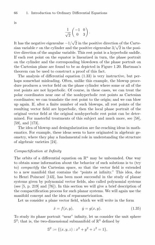
66 1. Introduction to Ordinary Differential Equations
is
1√2
(−1 00 3
).
It has the negative eigenvalue −1/√
2 in the positive direction of the Carte-sian variable r on the cylinder and the positive eigenvalue 3/
√2 in the posi-
tive direction of the angular variable. This rest point is a hyperbolic saddle.If each rest point on the equator is linearized in turn, the phase portraiton the cylinder and the corresponding blowdown of the phase portrait onthe Cartesian plane are found to be as depicted in Figure 1.20. Hartman’stheorem can be used to construct a proof of this fact.
The analysis of differential equation (1.33) is very instructive, but per-haps somewhat misleading. Often, unlike this example, the blowup proce-dure produces a vector field on the phase cylinder where some or all of therest points are not hyperbolic. Of course, in these cases, we can treat thepolar coordinates near one of the nonhyperbolic rest points as Cartesiancoordinates; we can translate the rest point to the origin; and we can blowup again. If, after a finite number of such blowups, all rest points of theresulting vector field are hyperbolic, then the local phase portrait of theoriginal vector field at the original nonhyperbolic rest point can be deter-mined. For masterful treatments of this subject and much more, see [58],[59], and [173].
The idea of blowup and desingularization are far-reaching ideas in math-ematics. For example, these ideas seem to have originated in algebraic ge-ometry, where they play a fundamental role in understanding the structureof algebraic varieties [24].
Compactification at Infinity
The orbits of a differential equation on Rn may be unbounded. One way
to obtain some information about the behavior of such solutions is to (tryto) compactify the Cartesian space, so that the vector field is extendedto a new manifold that contains the “points at infinity.” This idea, dueto Henri Poincare [143], has been most successful in the study of planarsystems given by polynomial vector fields, also called polynomial systems(see [5, p. 219] and [76]). In this section we will give a brief description ofthe compactification process for such planar systems. We will again use themanifold concept and the idea of reparametrization.
Let us consider a plane vector field, which we will write in the form
x = f(x, y), y = g(x, y). (1.35)
To study its phase portrait “near” infinity, let us consider the unit sphereS
2; that is, the two-dimensional submanifold of R3 defined by
S2 := (x, y, z) : x2 + y2 + z2 = 1,
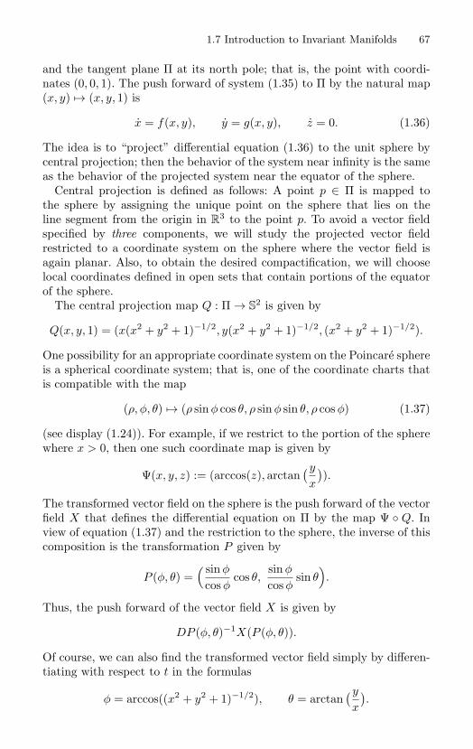
1.7 Introduction to Invariant Manifolds 67
and the tangent plane Π at its north pole; that is, the point with coordi-nates (0, 0, 1). The push forward of system (1.35) to Π by the natural map(x, y) → (x, y, 1) is
x = f(x, y), y = g(x, y), z = 0. (1.36)
The idea is to “project” differential equation (1.36) to the unit sphere bycentral projection; then the behavior of the system near infinity is the sameas the behavior of the projected system near the equator of the sphere.
Central projection is defined as follows: A point p ∈ Π is mapped tothe sphere by assigning the unique point on the sphere that lies on theline segment from the origin in R
3 to the point p. To avoid a vector fieldspecified by three components, we will study the projected vector fieldrestricted to a coordinate system on the sphere where the vector field isagain planar. Also, to obtain the desired compactification, we will chooselocal coordinates defined in open sets that contain portions of the equatorof the sphere.
The central projection map Q : Π → S2 is given by
Q(x, y, 1) = (x(x2 + y2 + 1)−1/2, y(x2 + y2 + 1)−1/2, (x2 + y2 + 1)−1/2).
One possibility for an appropriate coordinate system on the Poincare sphereis a spherical coordinate system; that is, one of the coordinate charts thatis compatible with the map
(ρ, φ, θ) → (ρ sin φ cos θ, ρ sin φ sin θ, ρ cos φ) (1.37)
(see display (1.24)). For example, if we restrict to the portion of the spherewhere x > 0, then one such coordinate map is given by
Ψ(x, y, z) := (arccos(z), arctan(y
x
)).
The transformed vector field on the sphere is the push forward of the vectorfield X that defines the differential equation on Π by the map Ψ Q. Inview of equation (1.37) and the restriction to the sphere, the inverse of thiscomposition is the transformation P given by
P (φ, θ) =( sin φ
cos φcos θ,
sin φ
cos φsin θ
).
Thus, the push forward of the vector field X is given by
DP (φ, θ)−1X(P (φ, θ)).
Of course, we can also find the transformed vector field simply by differen-tiating with respect to t in the formulas
φ = arccos((x2 + y2 + 1)−1/2), θ = arctan(y
x
).
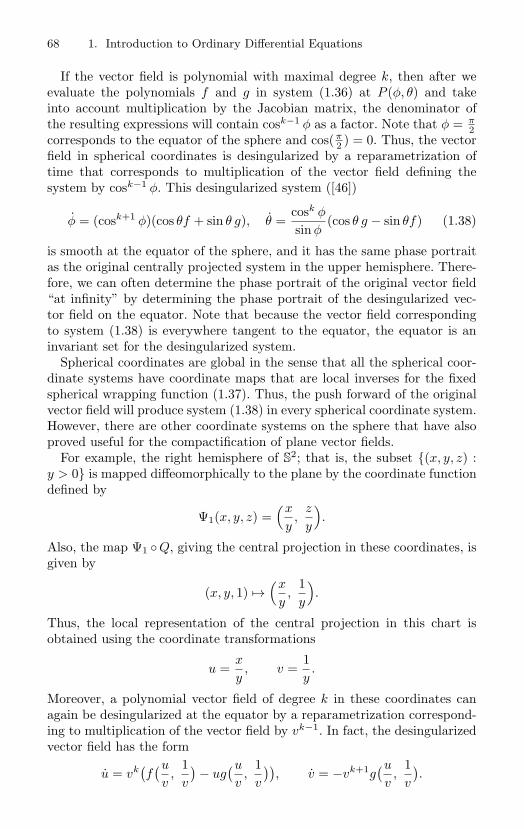
68 1. Introduction to Ordinary Differential Equations
If the vector field is polynomial with maximal degree k, then after weevaluate the polynomials f and g in system (1.36) at P (φ, θ) and takeinto account multiplication by the Jacobian matrix, the denominator ofthe resulting expressions will contain cosk−1 φ as a factor. Note that φ = π
2corresponds to the equator of the sphere and cos(π
2 ) = 0. Thus, the vectorfield in spherical coordinates is desingularized by a reparametrization oftime that corresponds to multiplication of the vector field defining thesystem by cosk−1 φ. This desingularized system ([46])
φ = (cosk+1 φ)(cos θf + sin θ g), θ =cosk φ
sin φ(cos θ g − sin θf) (1.38)
is smooth at the equator of the sphere, and it has the same phase portraitas the original centrally projected system in the upper hemisphere. There-fore, we can often determine the phase portrait of the original vector field“at infinity” by determining the phase portrait of the desingularized vec-tor field on the equator. Note that because the vector field correspondingto system (1.38) is everywhere tangent to the equator, the equator is aninvariant set for the desingularized system.
Spherical coordinates are global in the sense that all the spherical coor-dinate systems have coordinate maps that are local inverses for the fixedspherical wrapping function (1.37). Thus, the push forward of the originalvector field will produce system (1.38) in every spherical coordinate system.However, there are other coordinate systems on the sphere that have alsoproved useful for the compactification of plane vector fields.
For example, the right hemisphere of S2; that is, the subset (x, y, z) :
y > 0 is mapped diffeomorphically to the plane by the coordinate functiondefined by
Ψ1(x, y, z) =(x
y,
z
y
).
Also, the map Ψ1 Q, giving the central projection in these coordinates, isgiven by
(x, y, 1) →(x
y,
1y
).
Thus, the local representation of the central projection in this chart isobtained using the coordinate transformations
u =x
y, v =
1y.
Moreover, a polynomial vector field of degree k in these coordinates canagain be desingularized at the equator by a reparametrization correspond-ing to multiplication of the vector field by vk−1. In fact, the desingularizedvector field has the form
u = vk(f(u
v,
1v
)− ug
(u
v,
1v
)), v = −vk+1g
(u
v,
1v
).
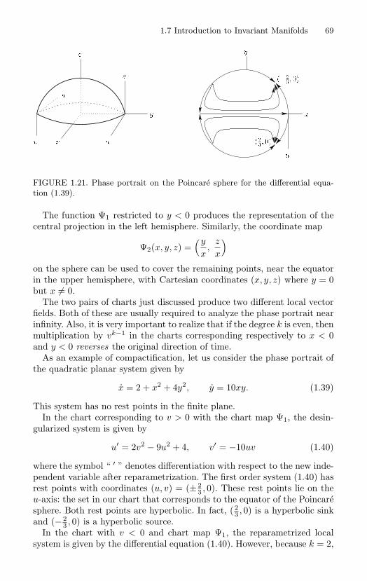
1.7 Introduction to Invariant Manifolds 69
y
v
z
uxv
u
x
u
y
FIGURE 1.21. Phase portrait on the Poincare sphere for the differential equa-tion (1.39).
The function Ψ1 restricted to y < 0 produces the representation of thecentral projection in the left hemisphere. Similarly, the coordinate map
Ψ2(x, y, z) =(y
x,
z
x
)on the sphere can be used to cover the remaining points, near the equatorin the upper hemisphere, with Cartesian coordinates (x, y, z) where y = 0but x = 0.
The two pairs of charts just discussed produce two different local vectorfields. Both of these are usually required to analyze the phase portrait nearinfinity. Also, it is very important to realize that if the degree k is even, thenmultiplication by vk−1 in the charts corresponding respectively to x < 0and y < 0 reverses the original direction of time.
As an example of compactification, let us consider the phase portrait ofthe quadratic planar system given by
x = 2 + x2 + 4y2, y = 10xy. (1.39)
This system has no rest points in the finite plane.In the chart corresponding to v > 0 with the chart map Ψ1, the desin-
gularized system is given by
u′ = 2v2 − 9u2 + 4, v′ = −10uv (1.40)
where the symbol “ ′ ” denotes differentiation with respect to the new inde-pendent variable after reparametrization. The first order system (1.40) hasrest points with coordinates (u, v) = (± 2
3 , 0). These rest points lie on theu-axis: the set in our chart that corresponds to the equator of the Poincaresphere. Both rest points are hyperbolic. In fact, (2
3 , 0) is a hyperbolic sinkand (− 2
3 , 0) is a hyperbolic source.In the chart with v < 0 and chart map Ψ1, the reparametrized local
system is given by the differential equation (1.40). However, because k = 2,
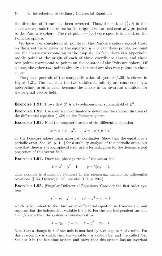
70 1. Introduction to Ordinary Differential Equations
the direction of “time” has been reversed. Thus, the sink at ( 23 , 0) in this
chart corresponds to a source for the original vector field centrally projectedto the Poincare sphere. The rest point (− 2
3 , 0) corresponds to a sink on thePoincare sphere.
We have now considered all points on the Poincare sphere except thoseon the great circle given by the equation y = 0. For these points, we mustuse the charts corresponding to the map Ψ2. In fact, there is a hyperbolicsaddle point at the origin of each of these coordinate charts, and theserest points correspond to points on the equator of the Poincare sphere. Ofcourse, the other two points already discussed are also rest points in thesecharts.
The phase portrait of the compactification of system (1.39) is shown inFigure 1.21. The fact that the two saddles at infinity are connected by aheteroclinic orbit is clear because the x-axis is an invariant manifold forthe original vector field.
Exercise 1.91. Prove that S2 is a two-dimensional submanifold of R
3.
Exercise 1.92. Use spherical coordinates to determine the compactification ofthe differential equation (1.39) on the Poincare sphere.
Exercise 1.93. Find the compactification of the differential equation
x = x + y − y3, y = −x + y + x3
on the Poincare sphere using spherical coordinates. Show that the equator is aperiodic orbit. See [46, p. 411] for a stability analysis of this periodic orbit, butnote that there is a typographical error in the formula given for the desingularizedprojection of this vector field.
Exercise 1.94. Draw the phase portrait of the vector field
x = x2 + y2 − 1, y = 5(xy − 1).
This example is studied by Poincare in his pioneering memoir on differentialequations ([143, Oeuvre, p. 66]; see also [107, p. 204]).
Exercise 1.95. [Singular Differential Equations] Consider the first order sys-tem
x′ = y, y′ = z, εz′ = y2 − xz − 1,
which is equivalent to the third order differential equation in Exercise 1.7, andsuppose that the independent variable is τ ∈ R. For the new independent variablet = τ/ε show that the system is transformed to
x = εy, y = εz, z = y2 − xz − 1.
Note that a change in t of one unit is matched by a change in τ of ε units. Forthis reason, if ε is small, then the variable τ is called slow and t is called fast.Set ε = 0 in the fast time system and prove that this system has an invariant
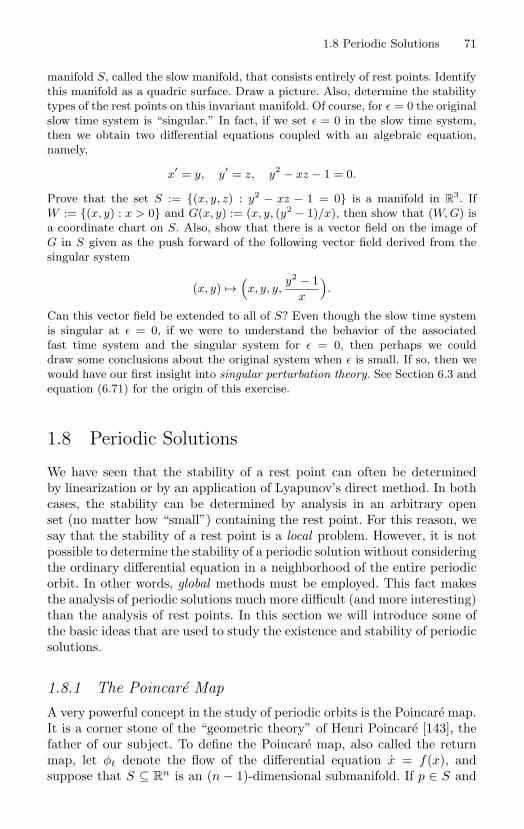
1.8 Periodic Solutions 71
manifold S, called the slow manifold, that consists entirely of rest points. Identifythis manifold as a quadric surface. Draw a picture. Also, determine the stabilitytypes of the rest points on this invariant manifold. Of course, for ε = 0 the originalslow time system is “singular.” In fact, if we set ε = 0 in the slow time system,then we obtain two differential equations coupled with an algebraic equation,namely,
x′ = y, y′ = z, y2 − xz − 1 = 0.
Prove that the set S := (x, y, z) : y2 − xz − 1 = 0 is a manifold in R3. If
W := (x, y) : x > 0 and G(x, y) := (x, y, (y2 − 1)/x), then show that (W, G) isa coordinate chart on S. Also, show that there is a vector field on the image ofG in S given as the push forward of the following vector field derived from thesingular system
(x, y) →(x, y, y,
y2 − 1x
).
Can this vector field be extended to all of S? Even though the slow time systemis singular at ε = 0, if we were to understand the behavior of the associatedfast time system and the singular system for ε = 0, then perhaps we coulddraw some conclusions about the original system when ε is small. If so, then wewould have our first insight into singular perturbation theory. See Section 6.3 andequation (6.71) for the origin of this exercise.
1.8 Periodic Solutions
We have seen that the stability of a rest point can often be determinedby linearization or by an application of Lyapunov’s direct method. In bothcases, the stability can be determined by analysis in an arbitrary openset (no matter how “small”) containing the rest point. For this reason, wesay that the stability of a rest point is a local problem. However, it is notpossible to determine the stability of a periodic solution without consideringthe ordinary differential equation in a neighborhood of the entire periodicorbit. In other words, global methods must be employed. This fact makesthe analysis of periodic solutions much more difficult (and more interesting)than the analysis of rest points. In this section we will introduce some ofthe basic ideas that are used to study the existence and stability of periodicsolutions.
1.8.1 The Poincare MapA very powerful concept in the study of periodic orbits is the Poincare map.It is a corner stone of the “geometric theory” of Henri Poincare [143], thefather of our subject. To define the Poincare map, also called the returnmap, let φt denote the flow of the differential equation x = f(x), andsuppose that S ⊆ R
n is an (n − 1)-dimensional submanifold. If p ∈ S and
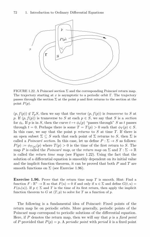
72 1. Introduction to Ordinary Differential Equations
x
S
p
P p
FIGURE 1.22. A Poincare section Σ and the corresponding Poincare return map.The trajectory starting at x is asymptotic to a periodic orbit Γ. The trajectorypasses through the section Σ at the point p and first returns to the section at thepoint P (p).
(p, f(p)) ∈ TpS, then we say that the vector (p, f(p)) is transverse to S atp. If (p, f(p)) is transverse to S at each p ∈ S, we say that S is a sectionfor φt. If p is in S, then the curve t → φt(p) “passes through” S as t passesthrough t = 0. Perhaps there is some T = T (p) > 0 such that φT (p) ∈ S.In this case, we say that the point p returns to S at time T . If there isan open subset Σ ⊆ S such that each point of Σ returns to S, then Σ iscalled a Poincare section. In this case, let us define P : Σ → S as follows:P (p) := φT (p)(p) where T (p) > 0 is the time of the first return to S. Themap P is called the Poincare map, or the return map on Σ and T : Σ → R
is called the return time map (see Figure 1.22). Using the fact that thesolution of a differential equation is smoothly dependent on its initial valueand the implicit function theorem, it can be proved that both P and T aresmooth functions on Σ (see Exercise 1.96).
Exercise 1.96. Prove that the return time map T is smooth. Hint: Find afunction F : R
n → R so that F (u) = 0 if and only if u ∈ Σ and define G(t, u) =F (φt(u)). If p ∈ Σ and T is the time of its first return, then apply the implicitfunction theorem to G at (T, p) to solve for T as a function of p.
The following is a fundamental idea of Poincare: Fixed points of thereturn map lie on periodic orbits. More generally, periodic points of thePoincare map correspond to periodic solutions of the differential equation.Here, if P denotes the return map, then we will say that p is a fixed pointof P provided that P (p) = p. A periodic point with period k is a fixed point
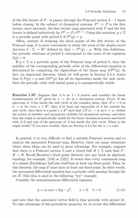
1.8 Periodic Solutions 73
of the kth iterate of P—it passes through the Poincare section k − 1 timesbefore closing. In the subject of dynamical systems, P 1 := P is the firstiterate; more precisely, the first iterate map associated with P and the kthiterate is defined inductively by P k := P P k−1. Using this notation, p ∈ Σis a periodic point with period k if P k(p) = p.
Often, instead of studying the fixed points of the kth iterate of thePoincare map, it is more convenient to study the zeros of the displacementfunction δ : Σ → R
n defined by δ(p) = P k(p) − p. With this definition,the periodic solutions of period k correspond to the roots of the equationδ(p) = 0.
If p ∈ Σ is a periodic point of the Poincare map of period k, then thestability of the corresponding periodic orbit of the differential equation isdetermined by computing the eigenvalues of the linear map DP k(p). Infact, an important theorem, which we will prove in Section 2.4.4, statesthat if P (p) = p and DP k(p) has all its eigenvalues inside the unit circle,then the periodic orbit with initial point p is asymptotically stable.
Exercise 1.97. Suppose that A is an 2 × 2 matrix and consider the lineartransformation of R
2 given by x → Ax as a dynamical system. Prove: If thespectrum of A lies inside the unit circle in the complex plane, then Akx → 0 ask → ∞ for every x ∈ R
2. Also, if at least one eigenvalue of A lies outside theunit circle, then there is a point x ∈ R
2 such that ||Akx|| → ∞ as k → ∞. Definethe notion of stability and asymptotic stability for dynamical systems, and showthat the origin is asymptotically stable for the linear dynamical system associatedwith A if and only if the spectrum of A lies inside the unit circle. When is theorigin stable? If you have trouble, then see Section 2.4.4 for the n × n case.
In general, it is very difficult to find a suitable Poincare section and toanalyze the associated Poincare map. However, there are many situationswhere these ideas can be used to great advantage. For example, supposethat there is a Poincare section Σ and a closed ball B ⊆ Σ such that P :B → B. Recall Brouwer’s fixed point theorem (see any book on algebraictopology, for example, [116] or [122]). It states that every continuous mapof a closed (Euclidean) ball into itself has at least one fixed point. Thus, bythis theorem, the map P must have at least one fixed point. In other words,the associated differential equation has a periodic orbit passing through theset B. This idea is used in the following “toy” example.
Consider the nonautonomous differential equation
y = (a cos t + b)y − y3, a > 0, b > 0 (1.41)
and note that the associated vector field is time periodic with period 2π.To take advantage of this periodicity property, let us recast this differential
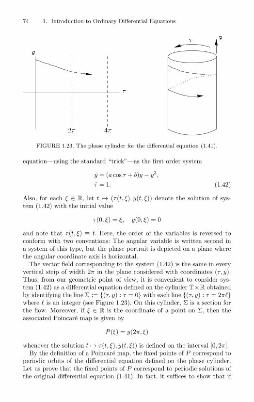
74 1. Introduction to Ordinary Differential Equations
y
y
FIGURE 1.23. The phase cylinder for the differential equation (1.41).
equation—using the standard “trick”—as the first order system
y = (a cos τ + b)y − y3,
τ = 1. (1.42)
Also, for each ξ ∈ R, let t → (τ(t, ξ), y(t, ξ)) denote the solution of sys-tem (1.42) with the initial value
τ(0, ξ) = ξ, y(0, ξ) = 0
and note that τ(t, ξ) ≡ t. Here, the order of the variables is reversed toconform with two conventions: The angular variable is written second ina system of this type, but the phase portrait is depicted on a plane wherethe angular coordinate axis is horizontal.
The vector field corresponding to the system (1.42) is the same in everyvertical strip of width 2π in the plane considered with coordinates (τ, y).Thus, from our geometric point of view, it is convenient to consider sys-tem (1.42) as a differential equation defined on the cylinder T×R obtainedby identifying the line Σ := (τ, y) : τ = 0 with each line (τ, y) : τ = 2πwhere is an integer (see Figure 1.23). On this cylinder, Σ is a section forthe flow. Moreover, if ξ ∈ R is the coordinate of a point on Σ, then theassociated Poincare map is given by
P (ξ) = y(2π, ξ)
whenever the solution t → τ(t, ξ), y(t, ξ)) is defined on the interval [0, 2π].By the definition of a Poincare map, the fixed points of P correspond to
periodic orbits of the differential equation defined on the phase cylinder.Let us prove that the fixed points of P correspond to periodic solutions ofthe original differential equation (1.41). In fact, it suffices to show that if
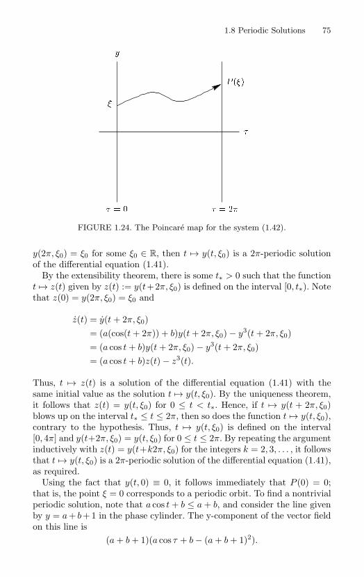
1.8 Periodic Solutions 75
P
y
FIGURE 1.24. The Poincare map for the system (1.42).
y(2π, ξ0) = ξ0 for some ξ0 ∈ R, then t → y(t, ξ0) is a 2π-periodic solutionof the differential equation (1.41).
By the extensibility theorem, there is some t∗ > 0 such that the functiont → z(t) given by z(t) := y(t+2π, ξ0) is defined on the interval [0, t∗). Notethat z(0) = y(2π, ξ0) = ξ0 and
z(t) = y(t + 2π, ξ0)= (a(cos(t + 2π)) + b)y(t + 2π, ξ0) − y3(t + 2π, ξ0)= (a cos t + b)y(t + 2π, ξ0) − y3(t + 2π, ξ0)= (a cos t + b)z(t) − z3(t).
Thus, t → z(t) is a solution of the differential equation (1.41) with thesame initial value as the solution t → y(t, ξ0). By the uniqueness theorem,it follows that z(t) = y(t, ξ0) for 0 ≤ t < t∗. Hence, if t → y(t + 2π, ξ0)blows up on the interval t∗ ≤ t ≤ 2π, then so does the function t → y(t, ξ0),contrary to the hypothesis. Thus, t → y(t, ξ0) is defined on the interval[0, 4π] and y(t+2π, ξ0) = y(t, ξ0) for 0 ≤ t ≤ 2π. By repeating the argumentinductively with z(t) = y(t+k2π, ξ0) for the integers k = 2, 3, . . . , it followsthat t → y(t, ξ0) is a 2π-periodic solution of the differential equation (1.41),as required.
Using the fact that y(t, 0) ≡ 0, it follows immediately that P (0) = 0;that is, the point ξ = 0 corresponds to a periodic orbit. To find a nontrivialperiodic solution, note that a cos t + b ≤ a + b, and consider the line givenby y = a+ b+1 in the phase cylinder. The y-component of the vector fieldon this line is
(a + b + 1)(a cos τ + b − (a + b + 1)2).
76 1. Introduction to Ordinary Differential Equations
Since
a cos τ + b − (a + b + 1)2 ≤ (a + b + 1) − (a + b + 1)2 < 0,
the vector field corresponding to the first order system “points” into theregion that lies below the line. In particular, if 0 ≤ ξ ≤ a + b + 1, then0 ≤ P (ξ) ≤ a + b + 1; that is, P maps the closed interval [0, a + b + 1] intoitself. Hence, the Brouwer fixed point theorem can be applied to prove theexistence of a periodic orbit (see also Exercise 1.98). But, because P (0) = 0,this application of the Brouwer fixed point theorem gives no informationabout the existence of nontrivial periodic solutions. The remedy, as we willsoon see, is to construct a P invariant closed interval that does not containξ = 0.
Suppose that P ′(0) > 1; that is, the trivial periodic solution is unstable.Then, there is some c > 0 such that 0 < c < a + b + 1 and P ′(ξ) > 1 aslong as 0 ≤ ξ ≤ c. By the mean value theorem, P (c) = P ′(ξ)c for someξ, 0 < ξ < c. Thus, P (c) > c. Using this inequality and the fact that Pis a Poincare map, it is easy to see that the interval c ≤ ξ ≤ a + b + 1 ismapped into itself by P and, as a result, there is at least one fixed pointin this interval. This fixed point corresponds to a periodic solution of thedifferential equation (1.41).
To prove that P ′(0) > 1 we will use a variational equation. This methodis employed very often in the analysis of differential equations. The presentelementary example is a good place to learn the basic technique. The idea issimple: The derivative of the solution of a differential equation with respectto its initial value is itself the solution of a differential equation.
Recall that P (ξ) = y(2π, ξ). Since
d
dty(t, ξ) = (a cos t + b)y(t, ξ) − y3(t, ξ)
we have that
d
dtyξ(t, ξ) = (a cos t + b)yξ(t, ξ) − 3y2(t, ξ)yξ(t, ξ).
Because y(0, ξ) = ξ, we also have the initial condition yξ(0, ξ) = 1. More-over, at the point ξ = 0 the function t → y(t, ξ) is identically zero. Thus, ift → w(t) is the solution of the variational initial value problem
w = (a cos t + b)w, w(0) = 1,
then P ′(0) = w(2π).Note that the variational differential equation is linear. Its solution is
given by
w(t) = e∫ t0 (a cos t+b) dt = ea sin t+bt.
1.8 Periodic Solutions 77
In particular, we have
P ′(0) = w(2π) = e2πb > 1,
as required. Moreover, this computation shows that the periodic solutiongiven by y(t) ≡ 0 is unstable. (Why?)
Exercise 1.98. Prove Brouwer’s fixed point theorem for a closed interval in R.Hint: Use the intermediate value theorem.
Exercise 1.99. Find the initial point for the nontrivial periodic solution in theinterval 0 < ξ < a + b + 1 for (1.41) as a function of a and b. Are there exactlytwo periodic solutions?
Exercise 1.100. Find conditions on a(t) and on f that ensure the existence ofat least one (nontrivial) periodic solution for a differential equation of the form
y = a(t)y + f(y).
Exercise 1.101. Consider the differential equation (1.41) on the cylinder, andthe transformation given by u = (y + 1) cos τ , v = (y + 1) sin τ that maps theportion of the cylinder defined by the inequality y > −1 into the plane. Whatis the image of this transformation? Find the differential equation in the newcoordinates, and draw its phase portrait.
We have proved that there is at least one 2π-periodic solution of thedifferential equation (1.41) with initial condition in the interval 0 < ξ <a + b + 1. But even more is true: This periodic orbit is stable and unique.To prove this fact, let us suppose that 0 < ξ0 < a + b + 1 and P (ξ0) = ξ0,so that the corresponding solution t → y(t, ξ0) is 2π-periodic.
To determine the stability type of the solution with initial value ξ0, itsuffices to compute P ′(ξ0). As before, P ′(ξ0) = w(2π) where t → w(t) isthe solution of the variational initial value problem
w = [(a cos t + b) − 3y2(t, ξ0)]w, w(0) = 1.
It follows that
P ′(ξ0) = w(2π)
= e∫ 2π0 a cos t+b−3y2(t,ξ0) dt
= e2πb−3∫ 2π0 y2(t,ξ0) dt.
To compute∫ 2π
0 y2 dt, note that because y(t, ξ0) > 0 for all t, we havethe following equality
y(t, ξ0)y(t, ξ0)
= a cos t + b − y2(t, ξ0).
78 1. Introduction to Ordinary Differential Equations
Using this formula and the periodicity of the solution t → y(t, ξ0), we havethat ∫ 2π
0y2(t, ξ0) dt = 2πb −
∫ 2π
0
y(t, ξ0)y(t, ξ0)
dt = 2πb,
and, as a result,
P ′(ξ0) = e2πb−3(2πb) = e−4πb < 1.
Hence, every periodic solution in the interval [0, a + b + 1] is stable. Theuniqueness of the periodic solution is a consequence of this result. In fact,the map P is real analytic. Thus, if P has infinitely many fixed pointsin a compact interval, then P is the identity. This is not true, so P hasonly a finite number of fixed points. If ξ0 and ξ1 are the coordinates oftwo consecutive fixed points, then the displacement function, that is, ξ →P (ξ) − ξ, has negative slope at two consecutive zeros, in contradiction.
Exercise 1.102. Find an explicit formula for the solution of the differentialequation (1.41) and use it to give a direct proof for the existence of a nontrivialperiodic solution.
Exercise 1.103. Is it possible for the Poincare map for a scalar differentialequation not to be the identity map on a fixed compact interval and at the sametime have infinitely many fixed points in the interval?
Exercise 1.104. Show that the (stroboscopic) Poincare map for the differentialequation (1.41) has exactly one fixed point on the interval (0, ∞). How many fixedpoints are there on (−∞, ∞)?
Exercise 1.105. Consider the second order differential equation
x + f(x)x + g(x) = 0
where f and g are 2π-periodic functions. Determine conditions on f and g thatensure the existence of a periodic solution.
Exercise 1.106. Compute the time required for the solution of the system
x = x(1 − y), y = y(x − 1)
with initial condition (x, y) = (1, 0) to arrive at the point (x, y) = (2, 0). Notethat this system has a section map y → h(y) defined from a neighborhood of(x, y) = (1, 0) on the line given by x = 1 to the line given by x = 2. Computeh′(0).
Exercise 1.107. Observe that the x-axis is invariant for the system
x = 1 + xy, y = 2xy2 + y3,
and the trajectory starting at the point (1, 0) crosses the line x = 3 at (3, 0).Thus, there is a section map h and a time-of-flight map T from the line x = 1 tothe line x = 3 with both functions defined on some open interval about the point(1, 0) on the line x = 1. Compute T ′(0) and h′(0).
1.8 Periodic Solutions 79
1.8.2 Limit Sets and Poincare–Bendixson TheoryThe general problem of finding periodic solutions for differential equationsis still an active area of mathematical research. Perhaps the most welldeveloped theory for periodic solutions is for differential equations definedon the plane. But, even in this case, the theory is far from complete. Forexample, consider the class of planar differential equations of the form
x = f(x, y), y = g(x, y)
where f and g are quadratic polynomials. There are examples of such“quadratic systems” that have four isolated periodic orbits—“isolated”means that each periodic orbit is contained in an open subset of the planethat contains no other periodic orbits (see Exercise 1.132). However, noone knows at present if there is a quadratic system with more than fourisolated periodic orbits. The general question of the number of isolatedperiodic orbits for a polynomial system in the plane has been open since1905; it is called Hilbert’s 16th problem (see [47], [97], [145], and [154]).
While there are certainly many difficult issues associated with periodicorbits of planar systems, an extensive theory has been developed that hasbeen successfully applied to help determine the dynamics of many mathe-matical models. Some of the basic results of this theory will be explainedlater in this section after we discuss some important general properties offlows of autonomous, not necessarily planar, systems.
The properties that we will discuss enable us to begin to answer thequestion “What is the long term behavior of a dynamical system?” Thisis often the most important question about a mathematical model. Askan engineer what he wants to know about a model ordinary differentialequation. Often his response will be the question “What happens if westart the system running and then wait for a long time?” or, in engineeringjargon, “What is the steady state behavior of the system?” We alreadyknow how to answer these questions in some special circumstances wherethe steady state behavior corresponds to a rest point or periodic orbit.However, we need the following definitions to precisely describe the limitingbehavior of an orbit.
Definition 1.108. Suppose that φt is a flow on Rn and p ∈ R
n. A point xin R
n is called an omega limit point (ω-limit point) of the orbit through p ifthere is a sequence of numbers t1 ≤ t2 ≤ t3 ≤ · · · such that limi→∞ ti = ∞and limi→∞ φti
(p) = x. The collection of all such omega limit points isdenoted ω(p) and is called the omega limit set (ω-limit set) of p. Similarly,the α-limit set α(p) is defined to be the set of all limits limi→∞ φti
(p) wheret1 ≥ t2 ≥ t3 ≥ · · · and limi→∞ ti = −∞.
Definition 1.109. The orbit of the point p with respect to the flow φt iscalled forward complete if t → φt(p) is defined for all t ≥ 0. Also, in thiscase, the set φt(p) : t ≥ 0 is called the forward orbit of the point p. The
80 1. Introduction to Ordinary Differential Equations
orbit is called backward complete if t → φt(p) is defined for all t ≤ 0 andthe backward orbit is φt(p) : t ≤ 0.
Proposition 1.110. If p ∈ Rn and the orbit of the flow φt through the
point p is forward complete, then ω(p) is a closed invariant set.
Proof. Suppose that x ∈ ω(p) and consider φT (x) for some fixed T > 0.There is a sequence t1 ≤ t2 ≤ t3 ≤ · · · with ti → ∞ and φti(p) → x asi → ∞. Note that t1 + T ≤ t2 + T ≤ t3 + T ≤ · · · and that φti+T (p) =φT (φti(p)). By the continuity of the flow, we have that φT (φti(p)) → φT (x)as i → ∞. Thus, φT (x) ∈ ω(p), and therefore ω(p) is an invariant set.
To show ω(p) is closed, it suffices to show that ω(p) is the intersection ofclosed sets. In fact, we have that
ω(p) =⋂τ≥0
closure φt(p) : t ≥ τ.
Proposition 1.111. Suppose that p ∈ Rn and the orbit of the flow φt
through the point p is forward complete. If the forward orbit of p has com-pact closure, then ω(p) is nonempty, compact, and connected.
Proof. The sequence φn(p)∞n=1 is contained in the compact closure of
the orbit through p. Thus, it has at least one limit point x. In fact, thereis an infinite sequence of integers n1 ≤ n2 ≤ · · · such that φni(p) → x asi → ∞. Hence, x ∈ ω(p), and therefore ω(p) = ∅.
Since ω(p) is a closed subset of the compact closure of the orbit throughp, the set ω(p) is compact.
To prove that ω(p) is connected, suppose to the contrary that thereare two disjoint open sets U and V whose union contains ω(p) such thatω(p) ∩ U = ∅ and ω(p) ∩ V = ∅. There is some t1 > 0 such that φt1(p) ∈ Uand some t2 > t1 such that φt2(p) ∈ V . But the set K = φt(p) : t1 ≤ t ≤t2 is the continuous image of an interval, hence a connected set. Thus Kcannot be contained in U ∪ V . In particular, there is at least one τ1 > 0such that φτ1(p) is not in this union.
Similarly we can construct a sequence τ1 ≤ τ2 ≤ · · · such that
limi→∞
τi = ∞
and for each i the point φτi(p) is in the complement of U ∪ V . By the
compactness, the sequence φτi(p)∞
i=1 has a limit point x. Clearly, x isalso in ω(p) and in the complement of U ∪ V . This is a contradiction.
Exercise 1.112. Construct examples to show that the compactness hypothesisof Proposition 1.111 is necessary.
Exercise 1.113. Suppose that x0 is a rest point for the differential equationx = f(x) with flow φt, and V is a Lyapunov function at x0. If, in addition, there
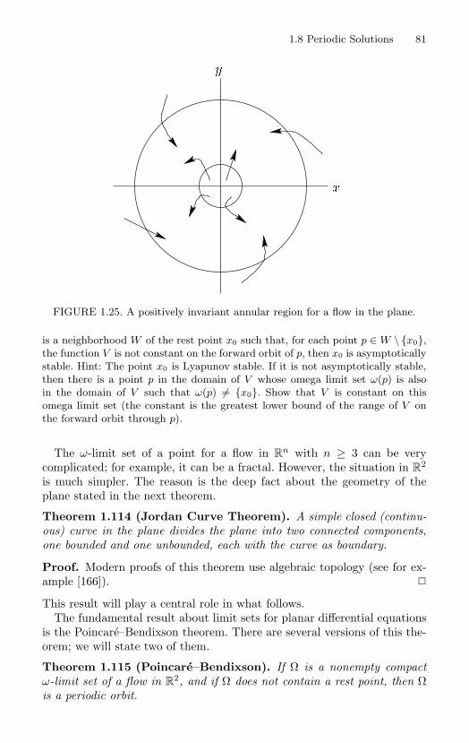
1.8 Periodic Solutions 81
y
x
FIGURE 1.25. A positively invariant annular region for a flow in the plane.
is a neighborhood W of the rest point x0 such that, for each point p ∈ W \ x0,the function V is not constant on the forward orbit of p, then x0 is asymptoticallystable. Hint: The point x0 is Lyapunov stable. If it is not asymptotically stable,then there is a point p in the domain of V whose omega limit set ω(p) is alsoin the domain of V such that ω(p) = x0. Show that V is constant on thisomega limit set (the constant is the greatest lower bound of the range of V onthe forward orbit through p).
The ω-limit set of a point for a flow in Rn with n ≥ 3 can be very
complicated; for example, it can be a fractal. However, the situation in R2
is much simpler. The reason is the deep fact about the geometry of theplane stated in the next theorem.
Theorem 1.114 (Jordan Curve Theorem). A simple closed (continu-ous) curve in the plane divides the plane into two connected components,one bounded and one unbounded, each with the curve as boundary.
Proof. Modern proofs of this theorem use algebraic topology (see for ex-ample [166]).
This result will play a central role in what follows.The fundamental result about limit sets for planar differential equations
is the Poincare–Bendixson theorem. There are several versions of this the-orem; we will state two of them.
Theorem 1.115 (Poincare–Bendixson). If Ω is a nonempty compactω-limit set of a flow in R
2, and if Ω does not contain a rest point, then Ωis a periodic orbit.
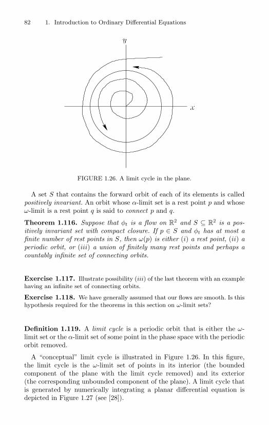
82 1. Introduction to Ordinary Differential Equations
y
x
FIGURE 1.26. A limit cycle in the plane.
A set S that contains the forward orbit of each of its elements is calledpositively invariant. An orbit whose α-limit set is a rest point p and whoseω-limit is a rest point q is said to connect p and q.
Theorem 1.116. Suppose that φt is a flow on R2 and S ⊆ R
2 is a pos-itively invariant set with compact closure. If p ∈ S and φt has at most afinite number of rest points in S, then ω(p) is either (i) a rest point, (ii) aperiodic orbit, or (iii) a union of finitely many rest points and perhaps acountably infinite set of connecting orbits.
Exercise 1.117. Illustrate possibility (iii) of the last theorem with an examplehaving an infinite set of connecting orbits.
Exercise 1.118. We have generally assumed that our flows are smooth. Is thishypothesis required for the theorems in this section on ω-limit sets?
Definition 1.119. A limit cycle is a periodic orbit that is either the ω-limit set or the α-limit set of some point in the phase space with the periodicorbit removed.
A “conceptual” limit cycle is illustrated in Figure 1.26. In this figure,the limit cycle is the ω-limit set of points in its interior (the boundedcomponent of the plane with the limit cycle removed) and its exterior(the corresponding unbounded component of the plane). A limit cycle thatis generated by numerically integrating a planar differential equation isdepicted in Figure 1.27 (see [28]).
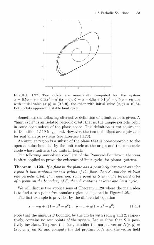
1.8 Periodic Solutions 83
-4 -2 0 2 4
-4
-2
0
2
4
FIGURE 1.27. Two orbits are numerically computed for the systemx = 0.5x − y + 0.1(x2 − y2)(x − y), y = x + 0.5y + 0.1(x2 − y2)(x + y): onewith initial value (x, y) = (0.5, 0), the other with initial value (x, y) = (0, 5).Both orbits approach a stable limit cycle.
Sometimes the following alternative definition of a limit cycle is given. A“limit cycle” is an isolated periodic orbit; that is, the unique periodic orbitin some open subset of the phase space. This definition is not equivalentto Definition 1.119 in general. However, the two definitions are equivalentfor real analytic systems (see Exercise 1.123).
An annular region is a subset of the plane that is homeomorphic to theopen annulus bounded by the unit circle at the origin and the concentriccircle whose radius is two units in length.
The following immediate corollary of the Poincare–Bendixson theoremis often applied to prove the existence of limit cycles for planar systems.
Theorem 1.120. If a flow in the plane has a positively invariant annularregion S that contains no rest points of the flow, then S contains at leastone periodic orbit. If in addition, some point in S is in the forward orbitof a point on the boundary of S, then S contains at least one limit cycle.
We will discuss two applications of Theorem 1.120 where the main ideais to find a rest-point free annular region as depicted in Figure 1.25.
The first example is provided by the differential equation
x = −y + x(1 − x2 − y2), y = x + y(1 − x2 − y2). (1.43)
Note that the annulus S bounded by the circles with radii 12 and 2, respec-
tively, contains no rest points of the system. Let us show that S is posi-tively invariant. To prove this fact, consider the normal vector N(x, y) =(x, y, x, y) on ∂S and compute the dot product of N and the vector field
84 1. Introduction to Ordinary Differential Equations
corresponding to the differential equation. In fact, the dot product
x2(1 − x2 − y2) + y2(1 − x2 − y2) = (x2 + y2)(1 − x2 − y2)
is positive on the circle with radius 12 and negative on the circle with radius
2. Therefore, S is positively invariant and, by Theorem 1.120, there is atleast one limit cycle in S.
The differential equation (1.43) is so simple that we can find a formulafor its flow. In fact, by changing to polar coordinates (r, θ), the transformedsystem
r = r(1 − r2), θ = 1
decouples, and its flow is given by
φt(r, θ) =(( r2e2t
1 − r2 + r2e2t
) 12, θ + t
). (1.44)
Note that φt(1, θ) = (1, θ + t) and, in particular, φ2π(1, θ) = (1, θ + 2π).Thus, the unit circle in the plane is a periodic orbit with period 2π. Here,of course, we must view θ as being defined modulo 2π, or, better yet, wemust view the polar coordinates as coordinates on the cylinder T × R (seeSection 1.7.4).
If the formula for the flow (1.44) is rewritten in rectangular coordinates,then the periodicity of the unit circle is evident. In fact, the periodic solu-tion starting at the point (cos θ, sin θ) ∈ R
2 (in rectangular coordinates) att = 0 is given by
t → (x(t), y(t)) = (cos(θ + t), sin(θ + t)).
It is easy to see that if r = 0, then the ω-limit set ω((r, θ)) is the entireunit circle. Thus, the unit circle is a limit cycle.
If we consider the positive x-axis as a Poincare section, then we have
P (x) =( x2e4π
1 − x2 + x2e4π
) 12.
Here P (1) = 1 and P ′(1) = e−4π < 1. In other words, the intersection pointof the limit cycle with the Poincare section is a hyperbolic fixed point ofthe Poincare map; that is, the linearized Poincare map has no eigenvalueon the unit circle of the complex plane. In fact, here the single eigenvalueof the linear transformation of R given by x → P ′(1)x is inside the unitcircle. It should be clear that in this case the limit cycle is an asymptoticallystable periodic orbit. We will also call such an orbit a hyperbolic stable limitcycle. (The general problem of the stability of periodic orbits is discussedin Chapter 2.)
1.8 Periodic Solutions 85
As a second example of the application of Theorem 1.120, let us considerthe very important differential equation,
θ + λθ + sin θ = µ
where λ > 0 and µ are constants, and θ is an angular variable; that is, θ isdefined modulo 2π. This differential equation is a model for an unbalancedrotor or pendulum with viscous damping λθ and external torque µ.
Consider the equivalent first order system
θ = v, v = − sin θ + µ − λv, (1.45)
and note that, since θ is an angular variable, the natural phase space forthis system is the cylinder T × R. With this interpretation we will showthe following result: If |µ| > 1, then system (1.45) has a globally attractinglimit cycle. The phrase “globally attracting limit cycle” means that thereis a limit cycle Γ on the cylinder and Γ is the ω-limit set of every point onthe cylinder. In other words, the steady state behavior of the unbalancedrotor, with viscous damping and sufficiently large torque, is stable periodicmotion. (See [109] for the existence of limit cycles for the case |µ| ≥ 1.)
The system (1.45) with |µ| > 1 has no rest points. (Why?) Also thequantity − sin θ + µ − λv is negative for sufficiently large positive valuesof v, and it is positive for negative values of v that are sufficiently largein absolute value. Therefore, there are numbers v− < 0 and v+ > 0 suchthat every forward orbit is contained in the compact subset of the cylinderA := (r, θ) : v− ≤ v ≤ v+. In addition, A is diffeomorphic to a closedannular region in the plane. It follows that the Poincare–Bendixson theoremis valid in A, and therefore the ω-limit set of every point on the cylinder isa limit cycle.
There are several ways to prove that the limit cycle is unique. However,let us consider a proof based on the following propositions: (i) If the diver-gence of a vector field is everywhere negative, then the flow of the vectorfield contracts volume (see Exercise 1.131). (ii) Every periodic orbit in theplane surrounds a rest point (see Exercise 1.127). (A replacement for thefirst proposition is given in Exercise 1.137.)
To apply the propositions, note that the divergence of the vector field forsystem (1.45) is the negative number −λ. Also, if |µ| > 1, then this systemhas no rest points. By the second proposition, no periodic orbit of thesystem is contractable on the cylinder (see panel (a) of Figure 1.28). Thus,if there are two periodic orbits, they must bound an invariant annularregion on the cylinder as in panel (b) of Figure 1.28. But this contradictsthe fact that the area of the annular region is contracted by the flow. Itfollows that there is a unique periodic orbit on the cylinder that is a globallyattracting limit cycle.
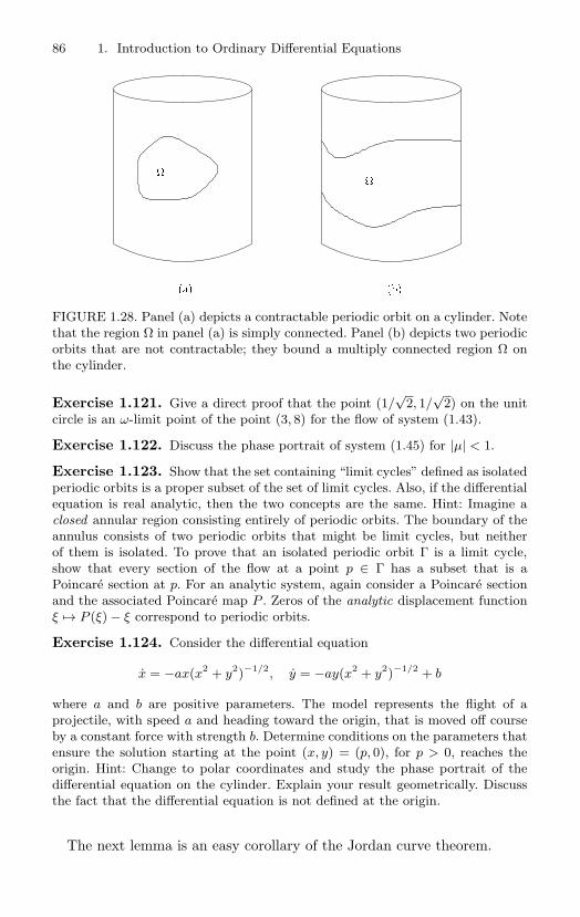
86 1. Introduction to Ordinary Differential Equations
ba
FIGURE 1.28. Panel (a) depicts a contractable periodic orbit on a cylinder. Notethat the region Ω in panel (a) is simply connected. Panel (b) depicts two periodicorbits that are not contractable; they bound a multiply connected region Ω onthe cylinder.
Exercise 1.121. Give a direct proof that the point (1/√
2, 1/√
2) on the unitcircle is an ω-limit point of the point (3, 8) for the flow of system (1.43).
Exercise 1.122. Discuss the phase portrait of system (1.45) for |µ| < 1.
Exercise 1.123. Show that the set containing “limit cycles” defined as isolatedperiodic orbits is a proper subset of the set of limit cycles. Also, if the differentialequation is real analytic, then the two concepts are the same. Hint: Imagine aclosed annular region consisting entirely of periodic orbits. The boundary of theannulus consists of two periodic orbits that might be limit cycles, but neitherof them is isolated. To prove that an isolated periodic orbit Γ is a limit cycle,show that every section of the flow at a point p ∈ Γ has a subset that is aPoincare section at p. For an analytic system, again consider a Poincare sectionand the associated Poincare map P . Zeros of the analytic displacement functionξ → P (ξ) − ξ correspond to periodic orbits.
Exercise 1.124. Consider the differential equation
x = −ax(x2 + y2)−1/2, y = −ay(x2 + y2)−1/2 + b
where a and b are positive parameters. The model represents the flight of aprojectile, with speed a and heading toward the origin, that is moved off courseby a constant force with strength b. Determine conditions on the parameters thatensure the solution starting at the point (x, y) = (p, 0), for p > 0, reaches theorigin. Hint: Change to polar coordinates and study the phase portrait of thedifferential equation on the cylinder. Explain your result geometrically. Discussthe fact that the differential equation is not defined at the origin.
The next lemma is an easy corollary of the Jordan curve theorem.
1.8 Periodic Solutions 87
Lemma 1.125. If Σ is a section for the flow φt and if p ∈ Σ, then theorbit through the point p intersects Σ in a monotone sequence; that is, ifφt1(p), φt2(p), φt3(p) all lie on Σ and if t1 < t2 < t3, then φt2(p) liesbetween φt1(p) and φt3(p) on Σ.
Proof. The proof is left as an exercise. Hint: Consider the curve formedby the union of φt(p) : t1 ≤ t ≤ t2 and the subset of Σ between φt1(p)and φt2(p). Draw a picture.
Corollary 1.126. If Σ is a section for the flow φt and if p ∈ Σ, thenω(p) ∩ Σ contains at most one point.
Proof. The proof is by contradiction. Suppose that ω(p) ∩ Σ contains atleast two points, x1 and x2. By rectification of the flow at x1 and at x2, thatis, by the rectification lemma (Lemma 1.76), it is easy to see that there aresequences φti
(p)∞i=1 and φsi
(p)∞i=1 in Σ such that limi→∞ φti
(p) = x1and limi→∞ φsi(p) = x2. The fact that such sequences can be found in Σfollows from the rectification lemma in Exercise 1.79. Indeed, we can choosethe rectifying neighborhood so that the image of the Poincare section is aline segment transverse to the rectified flow. In this case, it is clear thatif an orbit has one of its points in the rectifying neighborhood, then thisorbit passes through the Poincare section.
By choosing a local coordinate on Σ, let us assume that Σ is an openinterval. Working in this local chart, there are open subintervals J1 at x1and J2 at x2 such that J1∩J2 = ∅. Moreover, by the definition of limit sets,there is an integer m such that φtm
(p) ∈ J1; an integer n such that sn > tmand φsn
(p) ∈ J2; and an integer such that t > sn and φt(p) ∈ J1. By
Lemma 1.125, the point φsn(p) must be between the points φtm(p) andφt
(p) on Σ. But this is impossible because the points φtm(p) and φt(p)
are in J1, whereas φsn(p) is in J2.
We are now ready to prove the Poincare–Bendixson theorem (Theo-rem 1.115): If Ω is a nonempty compact ω-limit set of a flow in R
2, andif Ω does not contain a rest point, then Ω is a periodic orbit.
Proof. Suppose that ω(p) is compact and contains no rest points. Choosea point q ∈ ω(p). We will show first that the orbit through q is closed.
Consider ω(q). Note that ω(q) ⊆ ω(p) and let x ∈ ω(q). Since x is nota rest point, there is a section Σ at x and a sequence on Σ consisting ofpoints on the orbit through q that converges to x. These points are in ω(p).But, by the last corollary, this is impossible unless this sequence consistsof the singleton point x. Since q is not a rest point, this implies that q lieson a closed orbit Γ, as required. In particular, the limit set ω(p) containsthe closed orbit Γ.
To complete the proof we must show ω(p) ⊆ Γ. If ω(p) = Γ, then we willuse the connectedness of ω(p) to find a sequence pn∞
n=1 ⊂ ω(p) \ Γ thatconverges to a point z on Γ. To do this, consider the union A1 of all open
88 1. Introduction to Ordinary Differential Equations
balls with unit radius centered at some point in Γ. The set A1 \ Γ mustcontain a point in ω(p). If not, consider the union A1/2, (respectively A1/4)of all open balls with radius 1
2 (respectively 14 ) centered at some point in
Γ. Then the set A1/4 together with the complement of the closure of A1/2“disconnects” ω(p), in contradiction. By repeating the argument with ballswhose radii tend to zero, we can construct a sequence of points in ω(p) \ Γwhose distance from Γ tends to zero. Using the compactness of ω(p), thereis a subsequence, again denoted by pn∞
n=1, in ω(p) \ Γ that converges toa point z ∈ Γ.
Let U denote an open set at z such that the flow is rectified in a diffeo-morphic image of U . There is some integer n such that pn ∈ U . But, byusing the rectification lemma, it is easy to see that the orbit through pn
has a point y of intersection with some Poincare section Σ at z. Becausepn is not in Γ, the points y and z are distinct elements of the set ω(p) ∩ Σ,in contradiction to Corollary 1.126.
Exercise 1.127. Suppose that γ is a periodic orbit of a smooth flow definedon R
2. Prove that γ surrounds a rest point of the flow. That is, the boundedcomponent of the plane with the periodic orbit removed contains a rest point.
Exercise 1.128. Use Exercise 1.127 to prove the Brouwer fixed point theoremfor the closed unit disk D in R
2. Hint: First prove the result for a smooth func-tion f : D → D by considering the vector field f(x) − x, and then use the factthat a continuous transformation of D is the uniform limit of smooth transfor-mations [95, p. 253].
Exercise 1.129. Construct an example of a differential equation defined on allof R
3 that has a periodic orbit but no rest points.
Exercise 1.130. Prove: The ω-limit set of an orbit of a gradient system con-sists entirely of rest points.
Exercise 1.131. Prove: The flow of a vector field whose divergence is every-where negative contracts volume. Hint: If a vector field F on R
n with the usualEuclidean structure is given in components by F = (F1, F2, . . . , Fn), then
div F =n∑
i=1
∂Fi
∂xi.
Apply the change of variables formula for multiple integrals to an integral thatrepresents the volume of a region in R
n.
Exercise 1.132. Is a limit cycle isolated from all other periodic orbits? Hint:Consider planar vector fields of class C1 and those of class C ω—real analyticvector fields. Study the Poincare map on an associated transversal section.
Let us consider a result that can often be used to show that no periodicorbits exist.
1.8 Periodic Solutions 89
Proposition 1.133 (Bendixson’s Criterion). Consider a smooth dif-ferential equation on the plane
x = g(x, y), y = h(x, y)
and let f(x, y) := (g(x, y), h(x, y)). If the divergence of f given by
div f(x, y) := gx(x, y) + hy(x, y)
is not identically zero and of fixed sign in a simply connected region Ω, thenthe system has no periodic orbits in Ω.
Proof. Suppose that Γ is a closed orbit in Ω and let G denote the boundedregion of the plane bounded by Γ. Note that the line integral of the oneform g dy−h dx over Γ vanishes. (Why?) However, by Green’s theorem, theintegral can be computed by integrating the two-form (div f)dxdy over G.Since, by the hypothesis, the divergence of f does not vanish, the integralof the two-form over G does not vanish, in contradiction. Thus, no suchperiodic orbit can exist.
Theorem 1.134. Consider a smooth differential equation on the plane
x = g(x, y), y = h(x, y)
that has the origin as a rest point. Let J denote the Jacobian matrix forthe transformation (x, y) → (g(x, y), h(x, y)), and let φt denote the flow ofthe differential equation. If the following three conditions are satisfied, thenthe origin is globally asymptotically stable.
Condition 1. For each (x, y) ∈ R2, the trace of J given by gx(x, y) +
hy(x, y) is negative.Condition 2. For each (x, y) ∈ R
2, the determinant of J given bygx(x, y)hy(x, y) − gy(x, y)hx(x, y) is positive.
Condition 3. For each (x, y) ∈ R2, the forward orbit φt(x, y) : 0 ≤
t < ∞ is bounded.
Proof. From the hypotheses on the Jacobian matrix, if there is a rest point,the eigenvalues of its associated linearization all have negative real parts.Therefore, each rest point is a hyperbolic attractor; that is, the basin ofattraction of the rest point contains an open neighborhood of the rest point.This fact follows from Hartman’s theorem (Theorem 1.27) or Theorem 2.34.In particular, the origin is a hyperbolic attractor.
By the hypotheses, the trace of the Jacobian (the divergence of the vectorfield) is negative over the entire plane. Thus, by Bendixson’s criterion, thereare no periodic solutions.
Let Ω denote the basin of attraction of the origin. Using the continuityof the flow, it is easy to prove that Ω is open. In addition, it is easy toprove that the boundary of Ω is closed and contains no rest points.
90 1. Introduction to Ordinary Differential Equations
We will show that the boundary of Ω is positively invariant. If not, thenthere is a point p in the boundary and a time T > 0 such that either φT (p)is in Ω or such that φT (p) is in the complement of the closure of Ω inthe plane. In the first case, since φT (p) is in Ω, it is clear that p ∈ Ω, incontradiction. In the second case, there is an open set V in the complementof the closure of Ω that contains φT (p). The inverse image of V under thecontinuous map φT is an open set U containing the boundary point p. Bythe definition of boundary, U contains a point q ∈ Ω. But then, q is mappedto a point in the complement of the closure of Ω, in contradiction to thefact that q is in the basin of attraction of the origin.
If the boundary of Ω is not empty, consider one of its points. The(bounded) forward orbit through the point is precompact and containedin the (closed) boundary of Ω. Thus, its ω-limit set is contained in theboundary of Ω. Since the boundary of Ω contains no rest points, an ap-plication of the Poincare–Bendixson theorem shows this ω-limit set is aperiodic orbit, in contradiction. Thus, the boundary is empty and Ω is theentire plane.
Theorem 1.134 is a (simple) special case of the “Markus-Yamabe prob-lem.” In fact, the conclusion of the theorem is true without assuming Con-dition 3 (see [81]).
Exercise 1.135. Prove: If δ > 0, then the origin is a global attractor for thesystem
u = (u − v)3 − δu, v = (u − v)3 − δv.
Also, the origin is a global attractor of orbits in the first quadrant for the system
u = uv(u − v)(u + 1) − δu, v = vu(v − u)(v + 1) − δv.
(Both of these first order systems are mentioned in [181].)
Exercise 1.136. [Dulac’s Criterion] Recall the notation used in the state-ment of Bendixson’s criterion (Proposition 1.133). Prove Dulac’s generalizationof Bendixson’s criterion: If there is a smooth function B(x, y) defined on Ω suchthat the quantity (Bg)x + (Bh)y is not identically zero and of fixed sign on Ω,then there are no periodic orbits in Ω. Use Dulac’s criterion to prove a result dueto Nikolai N. Bautin: The system
x = x(a + bx + cy), y = y(α + βx + γy)
has no limit cycles. Hint: Look for a Dulac function of the form xrys.
Exercise 1.137. [Uniqueness of Limit Cycles] Prove the following proposition:If the divergence of a plane vector field is of fixed sign in an annular region Ω ofthe plane, then the associated differential equation has at most one periodic orbitin Ω. Hint: Use Green’s theorem. Also, recall Dulac’s criterion from Exercise 1.136and note that if the divergence of the plane vector field F is not of fixed sign in
1.8 Periodic Solutions 91
Ω, then it might be possible to find a nonnegative function B : Ω → R such thatthe divergence of BF does have fixed sign in Ω. As an example, consider the vander Pol oscillator,
x = y, y = −x + λ(1 − x2)y
and the “Dulac function” B(x, y) = (x2 + y2 − 1)−1/2. Show that van der Pol’ssystem has at most one limit cycle in the plane. (The remarkable Dulac function Bwas discovered by L. A. Cherkas.) Can you prove that the van der Pol oscillatorhas at least one limit cycle in the plane? Hint: Change coordinates using theLienard transformation
u = x, v = y − λ(x − 13x3)
to obtain the Lienard system
u = v + λ(u − 13u3), v = −u.
In Chapter 5 we will prove that the van der Pol system has a limit cycle if λ > 0is sufficiently small. However, this system has a limit cycle for each λ > 0. Forthis result, and for more general results about limit cycles of the important classof planar systems of the form
x = y − F (x), y = −g(x),
see [78, p. 154], [95, p. 215], [107, p. 267], and [141, p. 250].
Exercise 1.138. Prove that the system
x = x − y − x3, y = x + y − y3
has a unique globally attracting limit cycle on the punctured plane. Find all restpoints of the system
x = x − y − xn, y = x + y − yn,
where n is a positive odd integer and determine their stability. Prove that thesystem has a unique stable limit cycle. What is the limiting shape of the limitcycle as n → ∞?
Exercise 1.139. [Rigid Body Motion] The Euler equations for rigid body mo-tion are presented in Exercise 1.44. Recall that the momentum vector is given byM = AΩ where A is a symmetric matrix and Ω is the angular velocity vector,and Euler’s equation is given by M = M ×Ω. For ν a positive definite symmetricmatrix and F a constant vector, consider the differential equation
M = M × Ω + F − νM.
Here, the function M → νM represents viscous friction and F is the externalforce (see [14]). Prove that all orbits of the differential equation are bounded,and therefore every orbit has a compact ω-limit set.
92 1. Introduction to Ordinary Differential Equations
Exercise 1.140. Prove that the origin is a center for the system x+x2+x = 0.Also, show that this system has unbounded orbits. Is there a separatrix betweenthe bounded and unbounded solutions?
Exercise 1.141. Draw the phase portrait for the system x = x2 − x3. Is thesolution with initial conditions x(0) = 1
2 and x(0) = 0 periodic?
Exercise 1.142. Draw the phase portrait of the Hamiltonian system x + x −x2 = 0. Give an explicit formula for the Hamiltonian and use it to justify thefeatures of the phase portrait.
Exercise 1.143. Let t → x(t) denote the solution of the initial value problem
x + x + x + x3 = 0, x(0) = 1, x(0) = 0.
Determine limt→∞
x(t).
Exercise 1.144. Show that the system
x = x − y − (x2 +32y2)x, y = x + y − (x2 +
12y2)y
has a unique limit cycle.
Exercise 1.145. Find the rest points in the phase plane of the differentialequation x+(x2 +x2 −1)x+x = 0 and determine their stability. Also, show thatthe system has a unique stable limit cycle.
Exercise 1.146. Determine the ω-limit set of the solution of the system
x = 1 − x + y3, y = y(1 − x + y)
with initial condition x(0) = 10, y(0) = 0.
Exercise 1.147. Show that the system
x = −y + xy, y = x +12(x2 − y2)
has periodic solutions, but no limit cycles.
Exercise 1.148. Consider the van der Pol equation
x + (x2 − ε)x + x = 0,
where ε is a real parameter. How does the stability of the trivial solution changewith ε. Show that the van der Pol equation has a unique stable limit cycle forε = 1. What would you expect to happen to this limit cycle as ε shrinks to ε = 0.What happens for ε < 0?
Exercise 1.149. Find an explicit nonzero solution of the differential equation
t2x2x + x = 0.
Define new variables u = 2(3tx2)−1/2, v = −4x(3x3)−1/2 and show that
dv
du=
3v(v − u2)2u(v − u)
.
Draw the phase portrait of the corresponding first order system
u = 2u(v − u), v = 3v(v − u2).
1.9 Review of Calculus 93
1.9 Review of Calculus
The basic definitions of the calculus extend easily to multidimensionalspaces. In fact, these definitions are essentially the same when extendedto infinite dimensional spaces. Thus, we will begin our review with thedefinition of differentiation in a Banach space.
Definition 1.150. Let U be an open subset of a Banach space X, let Ydenote a Banach space, and let the symbol ‖ ‖ denote the norm in bothBanach spaces. A function f : U → Y is called (Frechet) differentiable ata ∈ U if there is a bounded linear operator Df(a) : X → Y , called thederivative of f , such that
limh→0
1‖h‖‖f(a + h) − f(a) − Df(a)h‖ = 0.
If f is differentiable at each point in U , then function f is called differen-tiable.
Using the notation of Definition 1.150, let L(X, Y ) denote the Banachspace of bounded linear transformations from X to Y , and note that thederivative of f : U → Y is the function Df : U → L(X, Y ) given byx → Df(x).
The following proposition is a special case of the chain rule.
Proposition 1.151. Suppose that U is an open subset of a Banach spaceand f : U → Y . If f is differentiable at a ∈ U and v ∈ U , then
d
dtf(a + tv)
∣∣t=0 = Df(a)v.
Proof. The proof is obvious for v = 0. Assume that v = 0 and considerthe scalar function given by
α(t) := ‖1t(f(a + tv) − f(a)) − Df(a)v)‖
=1|t| ‖f(a + tv) − f(a) − Df(a)tv‖
for t = 0. It suffices to show that limt→0 α(t) = 0.Choose ε > 0. Since f is differentiable, there is some δ > 0 such that
1‖h‖‖f(a + h) − f(a) − Df(a)h‖ < ε
whenever 0 < ‖h‖ < δ. If |t| < δ‖v‖−1, then ‖tv‖ < δ and
1|t|‖v‖‖f(a + tv) − f(a) − Df(a)tv‖ < ε.
In particular, we have that α(t) ≤ ‖v‖ε whenever |t| < δ‖v‖−1, as required.
94 1. Introduction to Ordinary Differential Equations
The following is a list of standard facts about the derivative; the proofsare left as exercises. For the statements in the list, the symbols X, Y , Xi,and Yi denote Banach spaces.
(i) If f : X → Y is differentiable at a ∈ X, then f is continuous at a.
(ii) If f : X → Y and g : Y → Z are both differentiable, then h = g fis differentiable, and its derivative is given by the chain rule
Dh(x) = Dg(f(x))Df(x).
(iii) If f : X → Y1 × · · · × Yn is given by f(x) = (f1(x), . . . , fn(x)), and iffi is differentiable for each i, then so is f and, in fact,
Df(x) = (Df1(x), . . . , Dfn(x)).
(iv) If the function f : X1×X2×· · ·×Xn → Y is given by (x1, . . . , xn) →f(x1, . . . , xn), then the ith partial derivative of f at a1, . . . , an ∈X1 × · · ·×Xn is the derivative of the function g : Xi → Y defined byg(xi) = f(a1, . . . , ai−1, xi, ai+1, . . . , an). This derivative is denotedDif(a). Of course, if f is differentiable, then its partial derivativesall exist and, if we define h = (h1, . . . , hn), we have
Df(x)h =n∑
i=1
Dif(x)hi.
Conversely, if all the partial derivatives of f exist and are continuousin an open set
U ⊂ X1 × X2 × · · · × Xn,
then f is continuously differentiable in U .
(v) If f : X → Y is a bounded linear map, then Df(x) = f for all x ∈ X.
The Cr-norm of an r-times continuously differentiable function f : U →Y , defined on an open subset U of X, is defined by
‖f‖r = ‖f‖0 + ‖Df‖0 + · · · ‖Drf‖0
where ‖ ‖0 denotes the usual supremum norm, as well as the operatornorms over U ; for example,
‖f‖0 = supu∈U
‖f(u)‖
and
‖Df‖0 = supu∈U
(sup
‖x‖=1‖Df(u)x‖
).
1.9 Review of Calculus 95
Also, let us use Cr(U, Y ) to denote the set of all functions f : U → Y suchthat ‖f‖r < ∞. Of course, the set Cr(U, Y ) is a Banach space of functionswith respect to the Cr-norm.
Although the basic definitions of differential calculus extend unchangedto the Banach space setting, this does not mean that there are no newphenomena in infinite dimensional spaces. The following examples and ex-ercises illustrate some of the richness of the theory. The basic idea is thatfunctions can be defined on function spaces in ways that are not availablein the finite dimensional context. If such a function is defined, then its dif-ferentiability class often depends on the topology of the Banach space in asubtle manner.
Example 1.152. Let X = C([0, 1]) and define F : X → X by
F (g)(t) := sin g(t)
(see [49]). We have the following proposition: The function F is continu-ously differentiable and
(DF (g)h)(t) = (cos g(t))h(t).
To prove it, let us first compute
|F (g + h)(t) − F (g)(t) − DF (g)h(t)|= | sin(g(t) + h(t)) − sin g(t) − (cos g(t))h(t)|= | sin g(t) cos h(t) + cos g(t) sin h(t) − sin g(t) − (cos g(t))h(t)|= |(−1 + cos h(t)) sin g(t) + (−h(t) + sin h(t)) cos g(t)|≤ ‖F (g)‖| − 1 + cos h(t)| + ‖ cos g‖| − h(t) + sin h(t)|
≤ 12(‖F (g)‖ ‖h‖2 + ‖ cos g‖ ‖h‖2).
This proves that F is differentiable.The function DF : X → L(X, X) given by g → DF (g) is clearly contin-
uous, in fact,
‖DF (g1) − DF (g2)‖ = sup‖h‖=1
‖DF (g1)h − DF (g2)h‖
= sup‖h‖=1
supt
|(cos g1(t))h(t) − (cos g2(t))h(t)|
≤ sup‖h‖=1
supt
|h(t)||g1(t) − g2(t)|
= ‖g1 − g2‖.
Thus F is continuously differentiable, as required.
Example 1.153. Let X := L2([0, 1]) and define F : X → X by
F (g)(t) = sin g(t).
96 1. Introduction to Ordinary Differential Equations
The function F is Lipschitz, but not differentiable.To prove that F is Lipschitz, simply recall that | sin x − sin y| ≤ |x − y|
and estimate as follows:
‖F (g1) − F (g2)‖2 =∫ 1
0| sin g1(t) − sin g2(t)|2 dt
≤∫ 1
0|g1(t) − g2(t)|2 dt
≤ ‖g1 − g2‖2.
We will show that F is not differentiable at the origin. To this end, letus suppose that F is differentiable at the origin with derivative DF (0). Wehave that F (0) = 0, and, by Proposition (1.151), all directional derivativesof F at the origin exist. Therefore, it follows that
lims→0
F (sg) − F (0)s
= lims→0
F (sg)s
= DF (0)g
for all g ∈ L2([0, 1]).To reach a contradiction, we will first prove that DF (0) is the identity
map on L2([0, 1]). To do this, it suffices to show that DF (0)g = g for everycontinuous function g ∈ L2([0, 1]). Indeed, this reduction follows becausethe (equivalence classes of) continuous functions are dense in L2([0, 1]).
Let us assume that g is continuous and square integrable. We will showthat the directional derivative of F at the origin in the direction g existsand is equal to g. In other words, we will show that
lims→0
F (sg)s
= g;
that is,
lims→0
∫ 1
0
∣∣∣ sin(sg(t))s
− g(t)∣∣∣2 ds = 0. (1.46)
Indeed, let us define
ψs(t) :=∣∣∣ sin(sg(t))
s− g(t)
∣∣∣2, s > 0
and note that
ψs(t) ≤(∣∣∣ sin(sg(t))
s
∣∣∣ + |g(t)|)2
.
Because | sin x| ≤ |x| for all x ∈ R, we have the estimates
ψs(t) ≤( |sg(t)|
|s| + |g(t)|)2
≤ 4|g(t)|2.
1.9 Review of Calculus 97
Moreover, the function t → 4|g(t)|2 is integrable, and therefore the functiont → ψs(t) is dominated by an integrable function.
If t is fixed, thenlims→0
ψs(t) = 0.
To prove this fact, let us observe that |g(t)| < ∞. If g(t) = 0, then ψs(t) = 0for all s and the result is clear. If g(t) = 0, then
ψs(t) =∣∣∣g(t)
( sin(sg(t))sg(t)
− 1)∣∣∣2
=∣∣∣g(t)
∣∣∣2∣∣∣ sin(sg(t))sg(t)
− 1∣∣∣2
and again ψs(t) → 0 as s → 0.We have proved that the integrand of the integral in display (1.46) is
dominated by an integrable function and converges to zero. Hence, therequired limit follows from the dominated convergence theorem and, more-over, DF (0)g = g for all g ∈ L2([0, 1]).
Because DF (0) is the identity map, it follows that
limh→0
‖F (h) − h‖‖h‖ = 0.
But let us consider the sequence of functions hn∞n=1 ⊂ L2([0, 1]) defined
by
hn(t) :=
π/2, 0 ≤ t ≤ 1/n,0, t > 1/n.
Since
‖hn‖ =(∫ 1
0(hn(t))2dt
)1/2=
( 1n
π2
4
)1/2=
1√n
π
2,
it follows that hn → 0 as n → ∞. Also, let us note that
‖F (hn) − hn‖ =(∫ 1
0| sin hn(t) − hn(t)|2dt
)1/2
=( 1
n
∣∣∣1 − π
2
∣∣∣2)1/2
and therefore
limn→∞
‖F (hn) − hn‖‖hn‖ = lim
n→∞
1√n(1 − π
2 )1√n
π2
=1 − π
2π2
= 0.
This contradiction proves that F is not differentiable at the origin. Is Fdifferentiable at any other point?
98 1. Introduction to Ordinary Differential Equations
Exercise 1.154. Consider the evaluation map
eval : Cr(U, Y ) × U → Y
defined by (f, u) → f(u). Prove that eval is a Cr map. Also, compute its deriva-tive.
Exercise 1.155. Suppose that f : R → R is a C2 function such that thequantity supx∈R
|f ′′(x)| is bounded. Prove that F : X → X as in Example 1.153is C1. The assumption that f is C2 can be replaced by the weaker hypothesisthat f is C1. This is a special case of the omega lemma (see [2, p. 101]). IfM is a compact topological space, U is an open subset of a Banach space X,and g is in Cr(U, Y ) where Y is a Banach space and r > 1, then the mapΩg : C0(M, U) → C0(M, Y ) given by Ωg(f) = g f is Cr and its derivativeis given by
(DΩg(f)h)(m) = Dg(f(m))h(m).
1.9.1 The Mean Value TheoremThe mean value theorem for functions of several variables is very important.However, the proof is somewhat more delicate than the usual proof for thecase of a scalar function of one variable. Let us begin with a special case.
Theorem 1.156. Suppose that [a, b] is a closed interval, Y is a Banachspace, and f : [a, b] → Y is a continuous function. If f is differentiableon the open interval (a, b) and there is some number M > 0 such that‖f ′(t)‖ ≤ M for all t ∈ (a, b), then
‖f(b) − f(a)‖ ≤ M(b − a).
Proof. Let ε > 0 be given and define φ : [a, b] → R by
φ(t) = ‖f(t) − f(a)‖ − (M + ε)(t − a).
Clearly, φ is a continuous function such that φ(a) = 0. We will show thatφ(b) ≤ ε.
Define S := t ∈ [a, b] : φ(t) ≤ ε. Since φ(a) = 0, we have that a ∈ S.In particular S = ∅. By the continuity of φ, there is some number c suchthat a < c < b and [a, c) ⊆ S. Moreover, since φ is continuous φ(t) → φ(c)as t → c. Thus, since φ(t) ≤ ε for a ≤ t < c, we must have φ(c) ≤ ε and, infact, [a, c] ⊆ S.
Consider the supremum c∗ of the set of all c such that a ≤ c ≤ b and[a, c] ⊆ S. Let us show that c∗ = b. If c∗ < b, then consider the derivativeof f at c∗ and note that because
lim‖h‖→0
‖f(c∗ + h) − f(c∗) − f ′(c∗)h‖‖h‖ = 0,
1.9 Review of Calculus 99
there is some h such that c∗ < c∗ + h < b and
‖f(c∗ + h) − f(c∗) − f ′(c∗)h‖ ≤ ε‖h‖.
Set d = c∗ + h and note that
‖f(d) − f(c∗)‖ ≤ ‖f(c∗ + h) − f(c∗) − f ′(c∗)h‖ + ‖f ′(c∗)h‖≤ ε‖h‖ + M‖h‖≤ (ε + M)(d − c∗).
Moreover, since
‖f(d) − f(a)‖ ≤ ‖f(d) − f(c∗)‖ + ‖f(c∗) − f(a)‖≤ (ε + M)(d − c∗) + (M + ε)(c∗ − a) + ε
≤ (ε + M)(d − a) + ε,
we have that‖f(d) − f(a)‖ − (ε + M)(d − a) ≤ ε,
and, as a result, d ∈ S, in contradiction to the fact that c∗ is the supremum.Thus, c∗ = b, as required.
Use the equality c∗ = b to conclude that
‖f(b) − f(a)‖ ≤ (ε + M)(b − a) + ε
≤ M(b − a) + ε(1 + (b − a))
for all ε > 0. By passing to the limit as ε → 0, we obtain the inequality
‖f(b) − f(a)‖ ≤ M(b − a),
as required.
Theorem 1.157 (Mean Value Theorem). Suppose that f : X → Y isdifferentiable on an open set U ⊆ X with a, b ∈ U and a + t(b − a) ∈ U for0 ≤ t ≤ 1. If there is some M > 0 such that
sup0≤t≤1
‖Df(a + t(b − a))‖ ≤ M,
then‖f(b) − f(a)‖ ≤ M‖b − a‖.
Proof. Define g(t) := f(a + t(b − a)). Clearly, g is differentiable on [0, 1]and, by the chain rule, g′(t) = Df(a + t(b − a))(b − a). In particular,
‖g′(t)‖ ≤ ‖Df(a + t(b − a))‖‖b − a‖ ≤ M‖b − a‖.
Here, g : [0, 1] → Y and ‖g′(t)‖ ≤ M‖b − a‖ for 0 ≤ t ≤ 1. By the previoustheorem,
‖g(1) − g(0)‖ ≤ M‖b − a‖,
that is,‖f(b) − f(a)‖ ≤ M‖b − a‖.
100 1. Introduction to Ordinary Differential Equations
1.9.2 Integration in Banach SpacesThis section is a brief introduction to integration on Banach spaces follow-ing the presentation in [106]. As an application, we will give an alternativeproof of the mean value theorem and a proof of a version of Taylor’s theo-rem.
Let I denote a closed interval of real numbers and X a Banach space withnorm ‖ ‖. A simple function f : I → X is a function with the followingproperty: There is a finite cover of I consisting of disjoint subintervals suchthat f restricted to each subinterval is constant. Here, each subinterval canbe open, closed, or half open.
A sequence fn∞n=1 of not necessarily simple functions, each mapping I
to X, converges uniformly to a function f : I → X if for each ε > 0 thereis an integer N > 0 such that ‖fn(t) − fm(t)‖ < ε whenever n, m > N andt ∈ I.
Definition 1.158. A regulated function is a uniform limit of simple func-tions.
Lemma 1.159. Every continuous function f : I → X is regulated.
Proof. The function f is uniformly continuous. To see this, consider F :I × I → X defined by F (x, y) = f(y)−f(x) and note that F is continuous.Since the diagonal D = (x, y) ∈ I × I : x = y is a compact subset ofI × I (Why?), its image F (D) is compact in X. Hence, for each ε > 0,a finite number of ε-balls in X cover the image of D. Taking the inverseimages of the elements of some such covering, we see that there is an opencover V1, . . . , Vn of the diagonal in I × I such that if (x, y) ∈ Vi, then‖F (x, y)‖ < ε. For each point (x, x) ∈ D, there is a ball centered at (x, x)and contained in I × I that is contained in some Vi. By compactness, afinite number of such balls cover D. Let δ denote the minimum radius ofthe balls in this finite subcover. If |x − y| < δ, then (x, y) ∈ Bδ(x, x) andin fact ‖(x, y) − (x, x)‖ = |y − x| < δ. Thus, (x, y) ∈ Vi for some i inthe set 1, . . . , n, and, as a result, we have that ‖F (x, y)‖ < ε; that is,‖f(y) − f(x)‖ = ‖F (x, y)‖ < ε, as required.
Let us suppose that I = x ∈ R : a ≤ x ≤ b. For each natural numbern, there is some δ > 0 such that if |x − y| < δ, then ‖f(x) − f(y)‖ < 1
n .Let us define a corresponding simple function fn by fn(x) = f(a) for a ≤x ≤ a + δ
2 , fn(x) = f(a + δ2 ) for a + δ
2 < x ≤ a + δ, fn(x) = f(a + δ) fora + δ < x ≤ a + 3δ
2 , and so on until a + k δ2 ≥ b. This process terminates
after a finite number of steps because I has finite length. Also, we have theinequality ‖fn(x) − f(x)‖ < 1
n for all x ∈ I. Thus, the sequence of simplefunctions fn∞
n=1 converges uniformly to f .
1.9 Review of Calculus 101
Definition 1.160. The integral of a simple function f : I → X over theinterval I = [a, b] is defined to be∫ b
a
f(t) dt :=n∑
j=1
µ(Ij)vj
where I1, . . . , In is a partition of I, f |Ij (t) ≡ vj , and µ(Ij) denotes thelength of the interval Ij .
Proposition 1.161. If f is a simple function on I, then the integral of fover I is independent of the choice of the partition of I.
Proof. The proof is left as an exercise.
Proposition 1.162. If f is a regulated function defined on the intervalI = [a, b], and if fn∞
n=1 is a sequence of simple functions converginguniformly to f , then the sequence defined by n →
∫ b
afn(t) dt converges
in X. Moreover, if in addition gn∞n=1 is a sequence of simple functions
converging uniformly to f , then
limn→∞
∫ b
a
fn(t) dt = limn→∞
∫ b
a
gn(t) dt.
Proof. We will show that the sequence n →∫ b
afn(t) dt is Cauchy. For this,
consider the quantity
‖∫ b
a
fn(t) dt −∫ b
a
fm(t) dt‖.
Using χL to denote the characteristic function on the interval L, we havethat, for some partitions of I and vectors vi and wi,
fn(x) =k∑
i=1
χIi(x)vi, fm(x) =
l∑i=1
χJi(x)wi.
The partitions I1, . . . , Ik and J1, . . . , Jl have a common refinement; thatis, there is a partition of the interval I such that each subinterval in thenew partition is contained in one of the subintervals I1, . . . , Ik, J1, . . . , Jl.Let this refinement be denoted by K1, . . . , Kp and note that
fn(x) =p∑
i=1
χKi(x)αi, fm(x) =
p∑i=1
χKi(x)βi.
Also, we have the inequality
‖∫ b
a
fn(t) dt −∫ b
a
fm(t) dt‖ = ‖p∑
i=1
µ(Ki)αi −p∑
i=1
µ(Ki)βi‖
≤p∑
i=1
µ(Ki)‖αi − βi‖.
102 1. Introduction to Ordinary Differential Equations
There are points ti ∈ Ki so thatp∑
i=1
µ(Ki)‖αi − βi‖ =p∑
i=1
µ(Ki)‖fn(ti) − fm(ti)‖
and, because∑p
i=1 µ(Ki) = b − a,p∑
i=1
µ(Ki)‖fn(ti) − fm(ti)‖ ≤ (b − a) maxi
‖fn(ti) − fm(ti)‖
≤ (b − a) maxx∈I
‖fn(x) − fm(x)‖.
By combining the previous inequalities and using the fact that the sequencefn∞
n=1 converges uniformly, it follows that the sequence n →∫ b
afn(t) dt
is a Cauchy sequence and thus converges to an element of X.Suppose that gn∞
n=1 is a sequence of simple functions that convergesuniformly to f , and let us suppose that∫ b
a
fn(t) dt → F,
∫ b
a
gn(t) dt → G.
We have the estimates
‖F − G‖ ≤ ‖F −∫ b
a
fn(t) dt‖ + ‖∫ b
a
fn dt −∫ b
a
gn dt‖ + ‖∫ b
a
gn dt − G‖
and
‖∫ b
a
fn dt −∫ b
a
gn dt‖ ≤ (b − a) maxx∈I
‖fn(x) − gn(x)‖
≤ (b − a) maxx∈I
(‖fn(x) − f(x)‖ + ‖f(x) − gn(x)‖).
The desired result, the equality F = G, follows by passing to the limit onboth sides of the previous inequality.
In view of the last proposition, we have the following basic definition:
Definition 1.163. Let f be a regulated function on the interval [a, b] andfn∞
n=1 a sequence of simple functions converging uniformly to f in X.The integral of f denoted
∫ b
af(t) dt is defined to be the limit of the sequence
n →∫ b
afn dt in X.
Proposition 1.164. The functional f →∫ b
af(t) dt, defined on the space
of regulated functions, is linear.
Proof. If f and g are regulated on the interval [a, b], with sequences ofsimple functions fn → f and gn → g, then cfn + dgn → cf + dg and∫ b
a
(cf + dg)(t) dt =∫ b
a
(cfn + dgn)(t) dt.
1.9 Review of Calculus 103
But, for these simple functions, after a common refinement,∫ b
a
cfn + dgn dt =n∑
i=1
µ(Ii)(cvi + dwi) = c
n∑i=1
µ(Ii)vi + d
n∑i=1
µ(Ii)wi.
Proposition 1.165. If λ : X → R is a continuous linear functional andif f : I → X is regulated, then the composition λf := λ f : I → R isregulated, and
λ
∫ b
a
f(t) dt =∫ b
a
(λf)(t) dt.
Proof. If fn∞n=1 is a sequence of simple functions converging uniformly
to f andfn(x) =
∑i
χIi(x)vi,
thenλ(fn(x)) =
∑i
χIi(x)λ(vi)
and, in particular, λfn is a simple function for each n. Moreover, λ f isregulated by λfn.
A continuous linear functional, by definition, has a bounded operatornorm. Therefore, we have that
|λfn(x) − λf(x)| = |λ(fn(x) − f(x))|≤ ‖λ‖‖fn(x) − f(x)‖
and∣∣∣λ ∫ b
a
f(t) dt −∫ b
a
λf(t) dt∣∣∣
≤∣∣∣λ ∫ b
a
f(t) dt − λ
∫ b
a
fn(t) dt∣∣∣ +
∣∣∣λ ∫ b
a
fn(t) dt −∫ b
a
λf(t) dt∣∣∣
≤ ‖λ‖‖∫ b
a
f(t) dt −∫ b
a
fn(t) dt‖ +∣∣∣ ∫ b
a
λfn(t) dt −∫ b
a
λf(t) dt∣∣∣.
The result follows by passing to the limit as n → ∞.
Proposition 1.166. If f : [a, b] → X is regulated, then
‖∫ b
a
f(t) dt‖ ≤ (b − a) supt∈[a,b]
‖f(t)‖. (1.47)
Proof. Note that the estimate (1.47) is true for simple functions; in fact,we have
‖∑
µ(Ii)vi‖ ≤∑
µ(Ii) sup(vi) ≤ (b − a)‖f‖.
104 1. Introduction to Ordinary Differential Equations
Because f is regulated, there is a sequence fn∞n=1 of simple functions
converging to f and, using this sequence, we have the following estimates:
‖∫ b
a
f(t) dt‖ ≤ ‖∫ b
a
f(t) dt −∫ b
a
fn(t) dt‖ + ‖∫ b
a
fn(t) dt‖
≤ ‖∫ b
a
f(t) dt −∫ b
a
fn(t) dt‖ + (b − a) supx
‖fn(x)‖
≤ ‖∫ b
a
f(t) dt −∫ b
a
fn(t) dt‖
+(b − a) supx
‖fn(x) − f(x)‖ + (b − a) supx
‖f(x)‖.
The desired result is obtained by passing to the limit as n → ∞.
Let us now apply integration theory to prove the mean value theorem. Wewill use the following proposition.
Proposition 1.167. Suppose that U is an open subset of X. If f : U → Yis a smooth function, and x + ty ∈ U for 0 ≤ t ≤ 1, then
f(x + y) − f(x) =∫ 1
0Df(x + ty)y dt. (1.48)
Proof. Let λ : Y → R be a continuous linear functional and consider thefunction F : [0, 1] → R given by
F (t) = λ(f(x + ty)) =: λf(x + ty).
The functional λ is C1 because it is linear. Also, the composition of smoothmaps is smooth. Thus, F is C1.
By the fundamental theorem of calculus, we have that
F (1) − F (0) =∫ 1
0F ′(t) dt,
or, equivalently,
λ(f(x + y) − f(x)) = λf(x + y) − λf(x)
=∫ 1
0λ(Df(x + ty)y) dt
= λ
∫ 1
0Df(x + ty)y dt.
Here, f(x + y) − f(x) and∫ 10 Df(x + ty)y dt are elements of Y , and λ has
the same value on these two points. Moreover, by our construction, thisis true for all continuous linear functionals. Thus, it suffices to prove the
1.9 Review of Calculus 105
following claim: If u, v are in X and λ(u) = λ(v) for all continuous linearfunctionals, then u = v. To prove the claim, set w = u − v and note thatZ := tw : t ∈ R is a closed subspace of Y . Moreover, λ0 : Z → R
defined by λ0(tw) = t‖w‖ is a linear functional on Z such that ‖λ0(tw)‖ =|t|‖w‖ = ‖tw‖. Thus, ‖λ0‖ = 1, and λ0 is continuous. By the Hahn–Banachtheorem, λ0 extends to a continuous linear functional λ on all of Y . But forthis extension we have, λ(w) = λ(1 · w) = ‖w‖ = 0. Thus, we have w = 0,and u = v.
With the same hypotheses as in Proposition 1.167, the mean value the-orem (Theorem 1.157) states that if x + t(z − x) ∈ U for 0 ≤ t ≤ 1, then
‖f(z) − f(x)‖ ≤ ‖z − x‖ supt∈[0,1]
‖Df(x + t(z − x))‖. (1.49)
Proof. By Proposition 1.167 we have that
‖f(z) − f(x)‖ = ‖∫ 1
0Df(x + t(z − x))(z − x) dt‖.
Also, the function t → Df(x + t(z − x))(z − x) is continuous. Thus, thedesired result is an immediate consequence of Lemma 1.159 and Proposi-tion 1.166.
The next theorem is a special case of Taylor’s theorem (see [2, p. 93] andExercise 1.169).
Theorem 1.168 (Taylor’s Theorem). Suppose that U is an open subsetof X. If f : U → Y is C1 and x + th ∈ U for 0 ≤ t ≤ 1, then
f(x + h) = f(x) + Df(x)h +∫ 1
0(Df(x + th)h − Df(x)h) dt.
Proof. By Proposition 1.167 we have
f(x + h) = f(x) +∫ 1
0Df(x + th)h dt
= f(x) +∫ 1
0((Df(x + th)h − Df(x)h) + Df(x)h) dt
= f(x) + Df(x)h +∫ 1
0(Df(x + th)h − Df(x)h) dt,
as required.
Exercise 1.169. Prove the following generalization of Theorem 1.168. Supposethat U is an open subset of X. If f : U → Y is Cr and x + th ∈ U for 0 ≤ t ≤ 1,
106 1. Introduction to Ordinary Differential Equations
then
f(x + h) = f(x) + Df(x)h + D2f(x)h2 + · · · Drf(x)hr
+∫ 1
0
(1 − t)r−1
(r − 1)!(Drf(x + th)hr − Drf(x)hr) dt.
1.9.3 The Contraction PrincipleIn this section, let us suppose that (X, d) is a metric space. A point x0 ∈ Xis a fixed point of a function T : X → X if T (x0) = x0. The fixed point x0is called globally attracting if limn→∞ Tn(x) = x0 for each x ∈ X.
Definition 1.170. Suppose that T : X → X, and λ is a real number suchthat 0 ≤ λ < 1. The function T is called a contraction (with contractionconstant λ) if
d(T (x), T (y)) ≤ λd(x, y)whenever x, y ∈ X.
The next theorem is fundamental; it states that a contraction, viewed asa dynamical system, has a globally attracting fixed point.
Theorem 1.171 (Contraction Mapping Theorem). If the function Tis a contraction on the complete metric space (X, d) with contraction con-stant λ, then T has a unique fixed point x0 ∈ X. Moreover, if x ∈ X, thenthe sequence Tn(x)∞
n=0 converges to x0 as n → ∞ and
d(Tn(x), x0) ≤ λn
1 − λd(x, x0).
Proof. Let us prove first that fixed points of T are unique. Indeed, ifT (x0) = x0 and T (x1) = x1, then, by virtue of the fact that T is a contrac-tion, d(T (x0), T (x1)) ≤ λd(x0, x1), and, by virtue of the fact that x0 andx1 are fixed points, d(T (x0), T (x1)) = d(x0, x1). Thus, we have that
d(x0, x1) ≤ λd(x0, x1).
If x0 = x1, then d(x0, x1) = 0 and therefore λ ≥ 1, in contradiction.To prove the existence of a fixed point, let x ∈ X and consider the
corresponding sequence of iterates Tn(x)∞n=1. By repeated applications
of the contraction property, it follows that
d(Tn+1(x), Tn(x)) ≤ λd(Tn(x), Tn−1(x)) ≤ · · · ≤ λnd(T (x), x).
Also, by using the triangle inequality together with this result, we obtainthe inequalities
d(Tn+p(x), Tn(x)) ≤ d(Tn+p(x), Tn+p−1(x)) + · · · + d(Tn+1(x), Tn(x))≤ (λn+p−1 + · · · + λn)d(T (x), x)≤ λn(1 + λ + · · · + λp−1)d(T (x), x)
≤ λn
1 − λd(T (x), x). (1.50)
1.9 Review of Calculus 107
Since 0 ≤ λ < 1, the sequence λn∞n=1 converges to zero, and therefore
Tn(x)∞n=1 is a Cauchy sequence. Thus, this sequence converges to some
point x0 ∈ X.We will prove that x0 is a fixed point of the map T . Let us first note
that, because the sequences Tn+1(x)∞n=0 and Tn(x)∞
n=1 are identical,limn→∞ Tn+1(x) = x0. Also, by the contraction property, it follows that Tis continuous and
d(Tn+1(x), T (x0)) = d(T (Tn(x)), T (x0)) ≤ λd(Tn(x), x0).
Therefore, using the continuity of T , we have the required limit
limn→∞ Tn+1(x) = lim
n→∞ T (Tn(x)) = T (x0).
To prove the estimate in the theorem, pass to the limit as p → ∞ in theinequality (1.50) to obtain
d(x0, Tn(x)) ≤ λn
1 − λd(T (x), x).
Exercise 1.172. Suppose that X is a set and n is a positive integer. Prove: IfT is a function, T : X → X, and if T n has a unique fixed point, then T has aunique fixed point.
For a contraction mapping depending on parameters, there is a uniformversion of the contraction principle.
Definition 1.173. Suppose that A is a set, T : X × A → X, and λ ∈ R issuch that 0 ≤ λ < 1. The function T is a uniform contraction if
d(T (x, a), T (y, a)) ≤ λd(x, y)
whenever x, y ∈ X and a ∈ A.
For uniform contractions in a Banach space where the metric is definedin terms of the Banach space norm by d(x, y) = ‖x − y‖, we have thefollowing result (see [49]).
Theorem 1.174 (Uniform Contraction Theorem). Suppose that Xand Y are Banach spaces, U ⊆ X and V ⊆ Y are open subsets, U denotesthe closure of U , the function T : U ×V → U is a uniform contraction withcontraction constant λ, and, for each y ∈ V , let g(y) denote the uniquefixed point of the contraction x → T (x, y) in U . If k is a non-negative in-teger and T ∈ Ck(U × V,X), then g : V → X is in Ck(V,X). Also, if T isreal analytic, then so is g.
108 1. Introduction to Ordinary Differential Equations
Proof. We will prove the theorem for k = 0, 1.By the definition of g given in the statement of the theorem, the identity
T (g(y), y) = g(y) holds for all y ∈ Y . If k = 0, then
‖g(y + h) − g(y)‖ = ‖T (g(y + h), y + h) − T (g(y), y)‖
≤ ‖T (g(y + h), y + h) − T (g(y), y + h)‖+ ‖T (g(y), y + h) − T (g(y), y)‖
≤ λ‖g(y + h) − g(y)‖ + ‖T (g(y), y + h) − T (g(y), y)‖,
and therefore
‖g(y + h) − g(y)‖ ≤ 11 − λ
‖T (g(y), y + h) − T (g(y), y)‖.
But T is continuous at the point (g(y), y). Thus, if ε > 0 is given, there issome δ > 0 such that
‖T (g(y), y + h) − T (g(y), y)‖ < ε whenever ‖h‖ < δ.
In other words, g is continuous, as required.Suppose that k = 1 and consider the function g : V → U given by
g(y) = T (g(y), y). We will prove that g is C1.The first observation is simple. If g is C1, then, by the chain rule,
Dg(y) = Tx(g(y), y)Dg(y) + Ty(g(y), y).
In other words, if Dg(y) exists, we expect it to be a solution of the equation
z = Tx(g(y), y)z + Ty(g(y), y). (1.51)
We will prove that, for each y ∈ V , the mapping
z → Tx(g(y), y)z + Ty(g(y), y),
on the Banach space of bounded linear transformations from Y to X, is acontraction. In fact, if z1 and z2 are bounded linear transformations fromY to X, then
‖Tx(g(y), y)z1 + Ty(g(y), y) − (Tx(g(y), y)z2 + Ty(g(y), y))‖≤ ‖Tx(g(y), y)‖‖z1 − z2‖.
Thus, the map is a contraction whenever ‖Tx(g(y), y)‖ < 1. In fact, as wewill soon see, ‖Tx(g(y), y)‖ ≤ λ. Once this inequality is proved, it followsfrom the contraction principle that for each y ∈ V the equation (1.51) hasa unique solution z(y). The differentiability of the the function y → g(y) isthen proved by verifying the limit
lim‖h‖→0
‖g(y + h) − g(y) − z(y)h‖‖h‖ = 0. (1.52)
1.9 Review of Calculus 109
To obtain the required inequality ‖Tx(g(y), y)‖ ≤ λ, let us use the factthat T is C1. In particular, the partial derivative Tx is a continuous functionand
lim‖h‖→0
‖T (x + h, y) − T (x, y) − Tx(x, y)h‖‖h‖ = 0.
Let ξ ∈ X be such that ‖ξ‖ = 1 and note that for each ε > 0, if we seth = εξ, then we have
‖Tx(x, y)ξ‖ = ‖1εTx(x, y)h‖
≤ 1ε
(‖T (x + h, y) − T (x, y) − Tx(x, y)h‖
+ ‖T (x + h, y) − T (x, y)‖)
=‖T (x + h, y) − T (x, y) − Tx(x, y)h‖
‖h‖ +λ‖h‖‖h‖ .
Passing to the limit as ε → 0, we obtain ‖Tx(x, y)ξ‖ ≤ λ, as required.To prove (1.52), set γ = γ(h) := g(y + h) − g(y). Since, g(y) is a fixed
point of the contraction mapping T , we have
γ = T (g(y) + γ, y + h) − T (g(y), y).
Set
∆ := T (g(y) + γ, y + h) − T (g(y), y) − Tx(g(y), y)γ − Ty(g(y), y)h
and note that
γ = T (g(y) + γ, y + h) − T (g(y), y) − Tx(g(y), y)γ−Ty(g(y), y)h + Tx(g(y), y)γ + Ty(g(y), y)h
= Tx(g(y), y)γ + Ty(g(y), y)h + ∆.
Also, since T is C1, we have for each ε > 0 a δ > 0 such that ‖∆‖ <ε(‖γ‖ + ‖h‖) whenever ‖γ‖ < δ and ‖h‖ < δ.
The function h → γ(h) is continuous. This follows from the first part ofthe proof since T ∈ C0. Thus, we can find δ1 > 0 so small that δ1 < δ and‖γ(h)‖ < δ whenever ‖h‖ < δ1, and therefore
‖∆(γ(h), h)‖ ≤ ε(‖γ(h)‖ + ‖h‖) whenever ‖h‖ < δ1.
For ‖h‖ < δ1, we have
‖γ(h)‖ = ‖Tx(g(y), y)γ + Ty(g(y), y)h + ∆(γ, y)‖
≤ λ‖γ‖ + ‖Ty(g(y), y)‖‖h‖ + ε(‖γ(h)‖ + ‖h‖)
110 1. Introduction to Ordinary Differential Equations
and, as a result,
(1 − λ − ε)‖γ(h)‖ ≤ (‖Ty(g(y), y)‖ + ε)‖h‖.
If we take ε < 1 − λ, then
‖γ(h)‖ ≤ 11 − λ − ε
(‖Ty(g(y), y)‖ + ε)‖h‖ := ψ‖h‖,
and it follows that
‖∆(γ(h), h)‖ ≤ ε(1 + ψ)‖h‖, ‖h‖ < δ1, 0 < ε < 1 − λ.
Finally, recall equation (1.51),
z = Tx(g(y), y)z + Ty(g(y), y),
and note that
(I − Tx(g(y), y))(γ(h) − z(y)h) = γ(h) − Tx(g(y), y)γ(h) − Ty(g(y), y)h= ∆(γ(h), h).
Also, since ‖Tx(g(y), y)‖ < λ < 1, we have
(I − Tx(g(y), y))−1 = I +∞∑
j=1
T jx
and‖(I − Tx(g(y), y))−1‖ ≤ 1
1 − ‖Tx‖ ≤ 11 − λ
.
This implies the inequality
‖γ(h) − z(y)h‖ ≤ ε
1 − λ(1 + ψ)‖h‖,
and the limit (1.52) follows.By our previous result about solutions of contractions being continuously
dependent on parameters, y → z(y) is continuous. This completes the proofof the theorem for the case k = 1.
Let us extend the contraction principle to bundles. The result of thisextension, called the fiber contraction theorem [93], is useful in proving thesmoothness of functions that are defined as fixed points of contractions.
Let X and Y denote metric spaces. A map Γ : X × Y → X × Y of theform
Γ(x, y) = (Λ(x), Ψ(x, y))
where Λ : X → X, and Ψ : X × Y → Y is called a bundle map overthe base Λ with principal part Ψ. Here, the triple (X × Y, X, π), whereπ : X × Y → X given by the projection π(x, y) = x, is called the trivialbundle over X with fiber Y .
1.9 Review of Calculus 111
Definition 1.175. Suppose that µ ∈ R is such that 0 ≤ µ < 1. Thebundle map Γ : X ×Y → X ×Y is called a fiber contraction if the functiony → Γ(x, y) is a contraction with contraction constant µ for every y ∈ Y .
Theorem 1.176 (Fiber Contraction Theorem). Suppose that X andY denote metric spaces, and that Γ : X ×Y → X ×Y is a continuous fibercontraction over Λ : X → X with principal part Ψ : X × Y → Y . If Λ hasa globally attracting fixed point x∞, and if y∞ is a fixed point of the mapy → Ψ(x∞, y), then (x∞, y∞) is a globally attracting fixed point of Γ.
Remark: The proof does not require the metric spaces X or Y to becomplete.
Proof. Let dX denote the metric for X, let dY denote the metric for Y ,and let the metric on X × Y be defined by d := dX + dY . We must showthat for each (x, y) ∈ X × Y we have limn→∞ Γn(x, y) = (x∞, y∞) wherethe limit is taken with respect to the metric d.
For notational convenience, let us denote the map y → Ψ(x, y) by Ψx.Then, for example, we have
Γn(x, y) = (Λn(x), ΨΛn(x) ΨΛn−1(x) · · · Ψx(y)),
and, using the triangle inequality, the estimate
d(Γn(x, y), (x∞, y∞)) ≤ d(Γn(x, y), Γn(x, y∞)) + d(Γn(x, y∞), (x∞, y∞)).(1.53)
Note that
d(Γn(x, y), Γn(x, y∞)) = dY (ΨΛn(x) ΨΛn−1(x) · · · Ψx(y),ΨΛn+1(x) ΨΛn(x) · · · Ψx(y∞)).
Moreover, if µ is the contraction constant for the fiber contraction Γ, thenwe have
d(Γn(x, y), Γn(x, y∞)) ≤ µndY (y, y∞).
Thus, d(Γn(x, y), Γn(x, y∞)) → 0 as n → ∞.For the second summand of (1.53), we have
d(Γn(x, y∞), (x∞, y∞)) ≤ dX(Λn(x), x∞) + dY (ΨΛn(x) · · · Ψx(y∞), y∞).
By the hypothesis that x∞ is a global attractor, the first summand on theright hand side of the last inequality converges to zero as n → ∞. Thus, tocomplete the proof, it suffices to verify the limit
limn→∞ dY (ΨΛn(x) ΨΛn−1(x) · · · Ψx(y∞), y∞) = 0. (1.54)
112 1. Introduction to Ordinary Differential Equations
Let us observe that
dY (ΨΛn(x) · · · Ψx(y∞), y∞) ≤ dY (ΨΛn(x) · · · Ψx(y∞), ΨΛn(x)(y∞))+dY (ΨΛn(x)(y∞), y∞)
≤ µdY (ΨΛn−1(x) · · · Ψx(y∞), y∞)+dY (ΨΛn(x)(y∞), y∞),
and by induction that
dY (ΨΛn(x) ΨΛn−1(x) · · · Ψx(y∞), y∞) ≤n∑
j=0
µn−jdY (ΨΛj(x)(y∞), y∞).
For each nonnegative integer m, define am := dY (ΨΛm(x)(y∞), y∞). Eacham is nonnegative and
am = dY (Ψ(Λm(x), y∞), Ψ(x∞, y∞)).
Using the continuity of Ψ and the hypothesis that x∞ is a globally attract-ing fixed point, it follows that the sequence am∞
m=0 converges to zeroand is therefore bounded. If A is an upper bound for the elements of thissequence, then for each m = 0, 1, . . . ,∞ we have 0 ≤ am < A.
Let ε > 0 be given. There is some K > 0 so large that
0 ≤ 12ak < (1 − µ)ε
whenever k ≥ K. Hence, if n ≥ K, then
n∑j=0
µn−jaj =K−1∑j=0
µn−jaj +n∑
j=K
µn−jaj
≤ AK−1∑j=0
µn−j +12(1 − µ)ε
n∑j=K
µn−j
≤ Aµn−K−1
1 − µ+
12ε.
Moreover, there is some N ≥ K such that
µn−K−1 <(1 − µ)ε
2A
whenever n ≥ N . In other words, limn→∞∑n
j=0 µn−jaj = 0.
As mentioned above, the fiber contraction principle is often used to provethat functions obtained as fixed points of contractions are smooth. We willuse this technique as one method to prove that the flow defined by a smooth
1.9 Review of Calculus 113
differential equation is smooth, and we will use a similar argument againwhen we discuss the smoothness of invariant manifolds. Thus, it seemsappropriate to codify the ideas that are used in these proofs to apply thefiber contraction principle. We will discuss a general guide to the analysisand a simple result to illustrate the procedure.
The setting for our analysis is given by a contraction Λ : C → C, where Cdenotes a closed subset of a Banach space of continuous functions that mapa Banach space X to a Banach space Y . Let α∞ ∈ C denote the uniquefixed point of Λ, and recall that α∞ is globally attracting; that is, if α ∈ C,then Λn(α) → α∞ as n → ∞.
Define the Banach space of all (supremum norm) bounded continuousfunctions from X to the linear maps from X to Y and denote this spaceby C(X, L(X, Y )). Elements of C(X, L(X, Y )) are the candidates for thederivatives of functions in C. Also, let C1 denote the subset of C consistingof all continuously differentiable functions with bounded derivatives.
The first step of the method is to show that if α ∈ C1, then the derivativeof Λ has the form
((DΛ)(α))(ξ) = Ψ(α, Dα)(ξ)
where ξ ∈ X and where Ψ is a map
Ψ : C × C(X, L(X, Y )) → C(X, L(X, Y )).
Next, define the bundle map
Λ : C × C(X, L(X, Y )) → C × C(X, L(X, Y ))
by
(α,Φ) → (Λ(α), Ψ(α,Φ))
and prove that Λ is a fiber contraction.Finally, pick a point α0 ∈ C1 so that (α0, Dα0) ∈ C(X, L(X, Y )), let
(φ0, Φ0) = (α0, Dα0), and define
(φn+1, Φn+1) = Λ(φn, Φn).
By the fiber contraction principle, the sequence given by (φn, Φn) convergesto (α∞, Φ∞) where Φ∞ ∈ C(X, L(X, Y )). By the construction of Ψ, ifn ≥ 0, then D(φn) = Φn. If the convergence is uniform (or at least uniformon compact subsets of X), then we obtain the desired result, D(α∞) = Φ∞,as an application of the following theorem from advanced calculus (seeExercise 1.181).
Theorem 1.177. If a sequence of differentiable functions is uniformlyconvergent and if the corresponding sequence of their derivatives is uni-formly convergent, then the limit function of the original sequence is dif-ferentiable and its derivative is the limit of the corresponding sequence ofderivatives.
114 1. Introduction to Ordinary Differential Equations
Moreover, we have Φ∞ ∈ C(X, L(X, Y )), and therefore Φ∞ is continuous.In particular, the fixed point α∞ is continuously differentiable.
We will state a simple result to illustrate a typical application of the fibercontraction principle. For this, let us consider specifically the linear spaceC0(RM , RN ) consisting of all continuous functions f : R
M → RN and let
C0(RM , RN ) denote the subspace consisting of all f ∈ C0(RM , RN ) suchthat the supremum norm is finite; that is,
‖f‖ := supξ∈RM
|f(ξ)| < ∞.
Of course, C0(RM , RN ) is a Banach space with the supremum norm. Also,let B0
ρ(RM , RN ) denote the subset of C0(RM , RN ) such that, for
f ∈ B0ρ(RM , RN ),
the Lipschitz constant of f is bounded by ρ; that is,
Lip(f) := supξ1 =ξ2
|f(ξ1) − f(ξ2)||ξ1 − ξ2|
≤ ρ.
It can be proved (see Exercise 1.180) that B0ρ(RM , RN ) is a closed subset of
C0(RM , RN ). It follows that B0ρ(RM , RN ) is a complete metric space with
respect to the supremum norm.If f ∈ C0(RM , RN ) and f is continuously differentiable with derivative
Df , then recall that Df is an element of the space C0(RM , L(RM , RN )),the space of continuous functions from R
M to the bounded linear mapsfrom R
M to RN . The subspace F of all such maps that are bounded with
respect to the norm
‖Φ‖ := supξ∈RN
(sup|v|=1
|Φ(ξ)v|),
is a Banach space. The subset Fρ of this space given by the closed metricball of radius ρ > 0 (that is, all Φ such that ‖Φ‖ ≤ ρ) is again a completemetric space relative to the norm just defined.
Theorem 1.178. If 0 < δ < 1 and F : RN → R
N is a continuouslydifferentiable function such that ‖F‖ < ∞ and ‖DF‖ < δ, then for eachnumber ρ with 0 < ρ < 1, the functional equation f = F f has a uniquesolution α in B0
ρ(RM , RN ). Moreover, α is continuously differentiable with‖Dα‖ < δ.
Proof. If f ∈ B0ρ(RM , RN ), then the function F f is continuous. Also,
we have that
‖F f‖ ≤ supξ∈RM
|F (f(ξ))| ≤ supζ∈RN
|F (ζ)| < ∞,
1.9 Review of Calculus 115
and, by the mean value theorem,
|F (f(ξ1)) − F (f(ξ2))| ≤ ‖DF‖|f(ξ1) − f(ξ2)| < δ Lip(f)|ξ1 − ξ2|;
that is, Lip(F f) < δ Lip(f) ≤ δρ < ρ. In other words, F f is an elementof the space B0
ρ(RM , RN ).Let us define Λ : B0
ρ(RM , RN ) → B0ρ(RM , RN ) by
Λ(f)(ξ) := F (f(ξ)),
and note that if f1 and f2 are in B0ρ(RM , RN ), then
|Λ(f1)(ξ) − Λ(f2)(ξ)| < δ‖f1 − f2‖;
that is, Λ is a contraction on the complete metric space B0ρ(RM , RN ). There-
fore, there is a unique function α ∈ B0ρ(RM , RN ) such that α = F α.
Moreover, if f ∈ B0ρ(RM , RN ), then limn→∞ Λn(f) = α.
It remains to prove that the function α is continuously differentiable. Tothis end, let us note that if φ ∈ B0
ρ(RM , RN ) and Φ ∈ Fρ, then
‖DF (φ(ξ))Φ(ξ)‖ < δρ < ρ.
Also, let us define a function Ψ : B0ρ(RM , RN ) × Fρ → Fρ by
Ψ(φ,Φ)(ξ) := DF (φ(ξ))Φ(ξ).
It follows that the function Φ → Ψ(φ,Φ) is a contraction on Fρ; in fact,
‖Ψ(φ,Φ1)(ξ) − Ψ(φ,Φ2)(ξ)‖ < δ‖Φ1 − Φ2‖.
In other words, the function
Λ : B0ρ(RM , RN ) × Fρ → B0
ρ(RM , RN ) × Fρ
given by
Λ(φ,Φ) := (Λ(φ),Ψ(φ,Φ))
is a fiber contraction.Let Φ∞ denote the unique fixed point of the contraction Φ → Ψ(α,Φ)
over the fixed point α. Also, let us define a sequence in B0ρ(RM , RN ) × Fρ
as follows: (φ0, Φ0) = (0, 0) and, for each positive integer n,
(φn+1, Φn+1) := Λ(φn, Φn).
Note that Dφ0 = Φ0 and, proceeding by induction, if Dφn = Φn, then
Dφn+1 = DΛ(φn) = DF (φn)Dφn = Ψ(φn, Dφn) = Ψ(φn, Φn) = Φn+1;
116 1. Introduction to Ordinary Differential Equations
that is, Dφn = Φn for all integers n ≥ 0.By the fiber contraction theorem, we have that
limn→∞ φn = α, lim
n→∞ Dφn = Φ∞.
The sequence φn∞n=0 converges uniformly to α and the sequence of its
derivatives converges uniformly to a limit. By Theorem 1.177 we have thatα is differentiable with derivative Φ∞. Thus, α is continuously differen-tiable.
Exercise 1.179. Let U denote an open ball in Rn or the entire space, and V
an open ball in Rm. Prove that the set of bounded continuous functions from U
to Rn is a Banach space, hence a complete metric space. Also, prove that the set
of continuous functions from U into V as well as the set of continuous functionsfrom V to R
n are Banach spaces.
Exercise 1.180. Prove that B0ρ(RM , R
N ) is a closed subset of the Banach spaceC0(RM , R
N ).
Exercise 1.181. Prove Theorem 1.177.
1.9.4 The Implicit Function TheoremThe implicit function theorem is one of the most useful theorems in analysis.We will prove it as a corollary of the uniform contraction theorem.
Theorem 1.182 (Implicit Function Theorem). Suppose that X, Y ,and Z are Banach spaces, U ⊆ X, V ⊆ Y are open sets, F : U×V → Z is aC1 function, and (x0, y0) ∈ U×V with F (x0, y0) = 0. If Fx(x0, y0) : X → Zhas a bounded inverse, then there is a product neighborhood U0×V0 ⊆ U×Vwith (x0, y0) ∈ U0×V0 and a C1 function β : V0 → U0 such that β(y0) = x0.Moreover, if F (x, y) = 0 for (x, y) ∈ U0 × V0, then x = β(y).
Proof. Define L : Z → X by Lz = [Fx(x0, y0)]−1z and G : U × V → Xby G(x, y) = x − LF (x, y). Note that G is C1 on U × V and F (x, y) = 0if and only if G(x, y) = x. Moreover, we have that G(x0, y0) = x0 andGx(x0, y0) = I − LFx(x0, y0) = 0.
Since G is C1, there is a product neighborhood U0 × V1 whose factorsare two metric balls, U0 ⊆ U centered at x0 and V1 ⊆ V centered at y0,such that
‖Gx(x, y)‖ <12
whenever (x, y) ∈ U0 × V1.Let us suppose that the ball U0 has radius δ > 0. Note that the function
given by y → F (x0, y) is continuous and vanishes at y0. Thus, there is a
1.10 Existence, Uniqueness, and Extensibility 117
metric ball V0 ⊆ V1 centered at y0 such that
‖L‖‖F (x0, y)‖ <δ
2
for every y ∈ V0. With this choice of V0, if (x, y) ∈ U0 × V0, then, by themean value theorem,
‖G(x, y) − x0‖ = ‖G(x, y) − G(x0, y) + G(x0, y) − x0‖≤ ‖G(x, y) − G(x0, y)‖ + ‖LF (x0, y)‖
≤ supu∈U1
‖Gx(u, y)‖‖x − x0‖ +δ
2≤ δ.
In other words, G(x, y) ∈ U0; that is, G : U0 × V0 → U0.Again, by the mean value theorem, it is easy to see that G is a uniform
contraction; in fact,
‖G(x1, y) − G(x2, y)‖ ≤ supu∈U1
‖Gx(u, y)‖‖x1 − x2‖
≤ 12‖x1 − x2‖.
Thus, there is a unique smooth function y → β(y) defined on the open ballV0 such that β(y0) = x0 and G(β(y), y) ≡ β(y). In particular,
β(y) = β(y) − LF (β(y), y)
and therefore F (β(y), y) ≡ 0, as required.
1.10 Existence, Uniqueness, and Extensibility
In this section we will prove the basic existence and uniqueness theorems fordifferential equations. We will also prove a theorem on extensibility of so-lutions. While the theorems on existence, uniqueness, and extensibility arethe foundation for theoretical study of ordinary differential equations, thereis another reason to study their proofs. In fact, the techniques used in thissection are very important in the modern development of our subject. Inparticular, the implicit function theorem is used extensively in perturbationtheory, and the various extensions of the contraction principle are funda-mental techniques used to prove the existence and smoothness of invariantmanifolds. We will demonstrate these tools by proving the fundamentalexistence theorem for differential equations in two different ways.
Suppose that J ⊆ R, Ω ⊆ Rn, and Λ ⊆ R
m are all open sets, and
f : J × Ω × Λ → Rn
118 1. Introduction to Ordinary Differential Equations
given by (t, x, λ) → f(t, x, λ) is a continuous function. Recall that if λ ∈ Λ,then a solution of the ordinary differential equation
x = f(t, x, λ) (1.55)
is a differentiable function σ : J0 → Ω defined on some open subintervalJ0 ⊆ J such that
dσ
dt(t) = f(t, σ(t), λ)
for all t ∈ J0. For t0 ∈ J , x0 ∈ Ω, and λ0 ∈ Λ, the initial value problemassociated with the differential equation (1.55) is given by the differentialequation together with an initial value for the solution as follows:
x = f(t, x, λ0), x(t0) = x0. (1.56)
If σ is a solution of the differential equation as defined above such that inaddition σ(t0) = x0, then we say that σ is a solution of the initial valueproblem (1.56).
Theorem 1.183. If the function f : J × Ω × Λ → Rn in the differential
equation (1.55) is continuously differentiable, t0 ∈ J , x0 ∈ Ω, and λ0 ∈Λ, then there are open sets J0 ⊆ J , Ω0 ⊆ Ω, and Λ0 ⊆ Λ such that(t0, x0, λ0) ∈ J0×Ω0×Λ0, and a unique C1 function σ : J0×Ω0×Λ0 → R
n
given by (t, x, λ) → σ(t, x, λ) such that t → σ(t, x0, λ0) is a solution of theinitial value problem (1.56).
Proof. The proof we will give is due to Joel Robbin [148]. Suppose thatσ is a solution of the initial value problem (1.56), δ > 0, and σ is definedon the interval [t0 − δ, t0 + δ]. In this case, if we define τ := (t − t0)/δ andz(τ) = σ(δτ + t0) − x0, then z(0) = 0 and for −1 ≤ τ ≤ 1,
dz
dτ(τ) = δσ(δτ + t0) = δf(δτ + t0, z + x0, λ0). (1.57)
Conversely, if the differential equation (1.57) has a solution defined ona subinterval of −1 ≤ τ ≤ 1, then the differential equation (1.55) hasa solution. Thus, it suffices to show the following proposition: If δ > 0 issufficiently small, then the differential equation (1.57) has a solution definedon the interval −1 ≤ τ ≤ 1.
Define the Banach spaces
X := φ ∈ C1([−1, 1], Rn) : φ(0) = 0, Y := C([−1, 1], Rn)
where the norm on Y is the usual supremum norm, the norm on X is givenby
‖φ‖1 = ‖φ‖ + ‖φ′‖,
and φ′ denotes the first derivative of φ. Also, define the function
F : K × J × Ω × Λ × X → Y
1.10 Existence, Uniqueness, and Extensibility 119
byF (δ, t, x, λ, φ)(τ) = φ′(τ) − δf(δτ + t, φ(τ) + x, λ).
We will apply the implicit function theorem to F .We will show that the function F is C1. Since the second summand in
the definition of F is C1, it suffices to show that the map d given by φ → φ′
is a C1 map from X to Y .Note that φ′ ∈ Y for each φ ∈ X and d is a linear transformation.
Because‖dφ‖ ≤ ‖dφ‖ + ‖φ‖ = ‖φ‖1,
the linear transformation d is continuous. Since the map d : X → Y islinear and bounded, it is its own derivative. In particular, d is continuouslydifferentiable.
If (t0, x0, λ0) ∈ J × Ω × Λ, then F (0, t0, x0, λ0, 0)(τ) = 0. Also, if we setδ = 0 before the partial derivative is computed, then it is easy to see that
Fφ(0, t0, x0, λ0, 0) = d.
In order to show that Fφ(0, t0, x0, λ0, 0) has a bounded inverse, it sufficesto show that d has a bounded inverse. To this end, define L : Y → X by
(Ly)(τ) =∫ τ
0y(s)ds.
Clearly,(d L) (y) = y and (L d) (ψ) = ψ.
Thus, L is an inverse for d. Moreover, since
‖Ly‖1 = ‖Ly‖ + ‖(d L)y‖
≤ ‖y‖ + ‖y‖ ≤ 2‖y‖,
it follows that L is bounded.By an application of the implicit function theorem to F , we have proved
the existence of a unique smooth function (δ, t, x, λ) → β(δ, t, x, λ), withdomain an open set K0 × J0 × Ω0 × Λ0 containing the point (0, t0, x0, λ0)and range in X such that β(0, t0, x0, λ0) = 0 and
F (δ, t, x, λ, β(δ, t, x, λ)) ≡ 0.
Thus, there is some δ > 0 such that
τ → z(τ, t0, x0, λ0) := β(δ, t0, x0, λ0)(τ)
is the required solution of the differential equation (1.57). Of course, thissolution depends smoothly on τ and all of its parameters.
120 1. Introduction to Ordinary Differential Equations
We will now consider a proof of Theorem 1.183 that uses the contractionprinciple and the fiber contraction theorem. For this, it is convenient tomake a minor change in notation and to introduce a few new concepts.
Instead of working directly with the initial value problem (1.56), we willstudy the solutions of initial value problems of the form
x = F (t, x), x(t0) = x0 (1.58)
where there is no dependence on parameters. In fact, there is no loss of gen-erality in doing so. Note that the initial value problem (1.56) is “equivalent”to the following system of differential equations:
y = f(t, y, λ), λ = 0, y(t0) = y0. (1.59)
In particular, if we define x = (y, λ) and F (t, (y, λ)) := (f(t, y, λ), 0), thensolutions of the initial value problem (1.56) can be obtained from solutionsof the corresponding initial value problem (1.58) in the obvious manner.Moreover, smoothness is preserved. Thus, it suffices to work with the initialvalue problem (1.58).
The existence of a local solution for the initial value problem (1.58) canbe proved using only the continuity of the function F . However, is F ismerely continuous, then a solution of the initial value problem may not beunique. A sufficient condition for uniqueness is the requirement that F isLipschitz with respect to its second argument; that is, there is a constantλ > 0 such that for each t ∈ J and for all x1, x2 ∈ Ω,
|f(t, x1) − f(t, x2)| ≤ λ|x1 − x2|
where |x| is the usual norm of x ∈ Rn. We will not prove the most general
possible result; rather we will prove the following version of Theorem 1.183.
Theorem 1.184. If the function F : J × Ω → Rn in the initial value
problem (1.58) is continuous and Lipschitz (with respect to its second ar-gument), t0 ∈ J , and x0 ∈ Ω, then there are open sets J0 ⊆ J andΩ0 ⊆ Ω such that (t0, x0) ∈ J0 × Ω0 and a unique continuous functionσ : J0 × Ω0 → R
n given by (t, x) → σ(t, x) such that t → σ(t, x0) is asolution of the initial value problem (1.58). If, in addition, F is C1, thenso is the function σ.
Proof. The function t → x(t) is a solution of the initial value problem ifand only if it is a solution of the integral equation
x(t) = x0 +∫ t
t0
F (s, x(s)) ds.
In fact, if dx/dt = F (t, x), then, by integration, we obtain the integralequation. On the other hand, if t → x(t) satisfies the integral equation,
1.10 Existence, Uniqueness, and Extensibility 121
then, by the fundamental theorem of calculus
dx
dt= F (t, x(t)).
Fix (t0, x0) ∈ J×Ω. Let b(t0, δ) and B(x0, ν) denote metric balls centeredat t0 and x0 with positive radii, respectively δ and ν, such that
b(t0, δ) × B(x0, ν) ⊆ J × Ω.
Since F is continuous on J × Ω, there is some number M > 0 such that
sup(t,x)∈b(t0,δ)×B(x0,ν)
|F (t, x)| ≤ M.
Since F is Lipschitz on J × Ω, there is some number λ > 0 such that, foreach t ∈ J and all x1, x2 ∈ Ω,
|F (t, x1) − F (t, x2)| ≤ λ|x1 − x2|.
If F ∈ C1 on J × Ω, then there is some number K > 0 such that
sup(t,x)∈b(t0,δ)×B(x0,ν)
‖DF (t, x)‖ ≤ K, (1.60)
where, recall, DF (t, x) is the derivative of the map x → F (t, x) and
‖DF (t, x)‖ := supv∈Rn:|v|=1
|DF (t, x)v|
with |x| the usual norm of x ∈ Rn.
Choose δ > 0 so that δλ < min(1, ν2 ) and δM < ν
2 , and define the Banachspace
X := C(b(t0, δ) × B(x0,ν
2), B(x0, ν))
with norm given by
‖φ‖ = sup(t,x)∈b(t0,δ)×B(x0, ν
2 )|φ(t, x)|.
In case F is C1, let us agree to choose δ as above, but with the additionalrestriction that δK < 1. Finally, define the operator Λ on X by
Λ(φ)(t, x) = x +∫ t
t0
F (s, φ(s, x)) ds. (1.61)
Let us prove that Λ : X → X. Clearly, we have Λ(φ) ∈ C(b(t0, δ) ×B(x0,
ν2 ), Rn). In view of the inequality
|Λ(φ)(t, x) − x0| ≤ |x − x0| +∫ t
t0
|F (s, φ(s, x))| ds
≤ |x − x0| + δM
<12ν +
12ν,
122 1. Introduction to Ordinary Differential Equations
the range of the operator Λ is in B(x0, ν), as required.The operator Λ is a contraction. In fact, if φ1, φ2 ∈ X, then
|Λ(φ1)(t, x) − Λ(φ2)(t, x)| ≤∫ t
t0
|F (s, φ1(s, x)) − F (s, φ2(s, x))| ds
≤ δλ‖φ1 − φ2‖,
and therefore‖Λ(φ1) − Λ(φ2)‖ ≤ δM‖φ1 − φ2‖,
as required. By the contraction principle, Λ has a unique fixed point. Thisfunction is a solution of the initial value problem (1.58) and it is continu-ously dependent on the initial condition.
If φ∞ denotes the fixed point of Λ, then ddtφ∞(t, x) = F (t, φ∞(t, x)). In
view of the fact that the functions φ∞ and F are continuous, it followsthat, for each fixed x ∈ B(x0,
ν2 ), the function t → φ∞(t, x) is C1. To
show that φ∞ is C1, it suffices to show that for each fixed t ∈ b(t0, δ)the function x → φ∞(t, x) is C1. We will prove this fact using the fibercontraction principle. The idea for this part of the proof is due to JorgeSotomayor [165].
Let us define a Banach space consisting of the “candidates” for the deriva-tives of functions in X with respect to their second arguments. To this end,let L(Rn, Rn) denote the set of linear transformations of R
n and define theBanach space
Y := C(b(t0, δ) × B(x0,ν
2), L(Rn, Rn))
consisting of all indicated functions that are bounded with respect to thenorm on Y given by
‖Φ‖ := sup(t,x)∈b(t0,δ)×B(x0, ν
2 )‖Φ(t, x)‖,
where, as defined above,
‖Φ(t, x)‖ := supv∈Rn:|v|=1
|Φ(t, x)v|.
Let I denote the identity transformation on Rn, DF (t, x) the derivative
of the map x → F (t, x), and define Ψ : X × Y → Y by
Ψ(φ,Φ)(t, x) := I +∫ t
t0
DF (s, φ(s, x))Φ(s, x) ds.
Also, define Γ : X × Y → X × Y by
Γ(φ,Φ) := (Λ(φ),Ψ(φ,Φ)).
1.10 Existence, Uniqueness, and Extensibility 123
To prove that Γ is a bundle map, is suffices to check that Γ is continuous.The proof of this fact uses the compactness of the interval b(t0, δ); thedetails are left to the reader.
Let us prove that Γ is a fiber contraction. Recall that we have chosen theradius of the time interval, δ > 0, so small that δK < 1, where the numberK is defined in equation (1.60). Using this fact, we have
‖Ψ(φ,Φ1)(t, x) − Ψ(φ,Φ2)(t, x)‖
= ‖∫ t
t0
DF (s, φ(s, x))(Φ1(s, x) − Φ2(s, x)) ds‖
< δK‖Φ1 − Φ2‖,
as required.Let φ0(t, x) ≡ x and note that (φ0, I) ∈ X × Y . By the fiber contraction
theorem (Theorem 1.176), the iterates of the point (φ0, I) under Γ convergeto a globally attracting fixed point, namely, (φ∞, Φ∞), where in this caseφ∞ is the solution of the initial value problem (the fixed point of Λ) andΦ∞ is the unique fixed point of the contraction Φ → Ψ(φ∞, Φ) on Y .
We will prove that Dφ∞(t, ·) = Φ∞(t, ·). (The derivative denoted byD is the partial derivative with respect to the second variable.) Let usstart with the equation Dφ0(t, x) = I, and for each integer n > 1 define(φn, Φn) := Γn(φ0, I) so that
Φn+1(t, x) = Ψ(φn, Φn)(t, x) := I +∫ t
t0
DF (s, φn(s, x))Φn(s, x) ds,
φn+1(t, x) = x +∫ t
t0
F (s, φn(s, x)) ds.
Let us show the identity Dφn(t, ·) = Φn(t, ·) for each integer n ≥ 0. Theequation is true for n = 0. Proceeding by induction on n, let us assumethat the equation is true for some fixed integer n ≥ 0. Then, using the factthat we can “differentiate under the integral,” the derivative
Dφn+1(t, x) =∂
∂x(x +
∫ t
t0
F (s, φn(s, x)) ds)
is clearly equal to
I +∫ t
t0
DF (s, φn(s, x))Φn(s, x) ds = Φn+1(t, x),
as required. Thus, we have proved that the sequence Dφn(t, ·)∞n=0 con-
verges to Φ∞(t, ·). Finally, by Theorem 1.177 we have that Dφ∞(t, ·) =Φ∞(t, ·).
124 1. Introduction to Ordinary Differential Equations
Exercise 1.185. It is very easy to show that a C2 differential equation has aC1 flow. Why? We have proved above the stronger result that a C1 differentialequation has a C1 flow. Show that a Cr differential equation has a Cr flow forr = 2, 3, . . . , ∞. Also, show that a real analytic differential equation has a realanalytic flow.
So far we have proved that initial value problems have unique solutionsthat exist on some (perhaps small) interval containing the initial time. If wewish to find a larger interval on which the solution is defined, the followingproblem arises. Suppose that the initial value problem
x = f(t, x), x(t0) = x0
has a solution t → φ(t) defined on some interval J containing t0. Maybethe solution is actually defined on some larger time interval J1 ⊇ J . If wehave a second solution ψ(t) defined on J1, then, by our local uniquenessresult, ψ(t) = φ(t) on J . But, we may ask, does ψ(t) = φ(t) on J1? Theanswer is yes.
To prove this fact, consider all the open intervals containing J . The unionof all such intervals on which φ(t) = ψ(t) is again an open interval J∗; itis the largest open interval on which φ and ψ agree. Let us prove thatJ∗ ⊇ J1. If not, then the interval J∗ has an end point t1 ∈ J1 that is notan endpoint of J1. Suppose that t1 is the right hand endpoint of J∗. Bycontinuity,
φ(t1) = ψ(t1).
Thus, by our local existence theorem, there is a unique solution of theinitial value problem
x = f(t, x), x(t1) = φ(t1)
defined in some neighborhood of t1. It follows that φ(t) = ψ(t) on somelarger interval. This contradiction implies that J∗ ⊇ J1, as required. Inparticular, if a solution extends, then it extends uniquely.
Our existence theorem for solutions of initial value problems gives noinformation about the length of the maximal interval of existence. In fact,the exact domain on which a given solution is defined is usually very difficultto determine. We will formulate and prove an abstract theorem in thisdirection that is often useful. However, before formulating this result, letus recall that even if the vector field associated with a differential equationhas no singularities, solutions of the differential equation may not existfor all t ∈ R. The classic example (already mentioned) is the initial valueproblem
x = x2, x(0) = 1.
The maximal interval of existence of the solution x(t) = (1 − t)−1 is theinterval (−∞, 1). Moreover, this solution blows up in finite time, that is,
1.10 Existence, Uniqueness, and Extensibility 125
x(t) → ∞ as t → 1−. Following the presentation in [95], the next theoremshows that our example illustrates the typical behavior.
Theorem 1.186. Let U ⊆ Rn and J ⊆ R be open sets such that the open
interval (α, β) is contained in J . Also, let x0 ∈ U . If f : J × U → Rn is a
C1 function and the maximal interval of existence of the solution t → φ(t)of the initial value problem x = f(t, x), x(t0) = x0 is α < t0 < β withβ < ∞, then for each compact set K ⊂ U there is some t ∈ (α, β) such thatφ(t) ∈ K. In particular, either |φ(t)| becomes unbounded or φ(t) approachesthe boundary of U as t → β.
Proof. Suppose that the solution φ has maximal interval of existence (α, β)with β < ∞ and K is a compact subset of U such that φ(t) ∈ K for allt ∈ (α, β). We will show that under these assumptions the interval (α, β)is not maximal.
The set [t0, β] × K is compact. Thus, there is some M > 0 such that|f(t, x)| < M for each (t, x) ∈ [t0, β] × K. Moreover, the function φ :[t0, β) → K is continuous.
We will show that the function φ extends continuously to the interval[t0, β]. Note first that φ is uniformly continuous on [t0, β). In fact, if s1, s2 ∈[t0, β) and s1 < s2, then
|φ(s2) − φ(s1)| =∣∣∣ ∫ s2
s1
f(t, φ(t)) dt∣∣∣ ≤ M |s2 − s1|. (1.62)
A standard theorem from advanced calculus states that φ extends contin-uously to [t0, β]. However, for completeness we will prove this fact for ourspecial case.
Construct a sequence tn∞n=1 of numbers in the interval [t0, β) that
converges to β, and recall that a convergent sequence is Cauchy. By in-equality (1.62), the sequence φ(tn)∞
n=1 is also Cauchy. Hence, there issome ω ∈ R such that φ(tn) → ω as n → ∞.
Let us extend the function φ to the closed interval [t0, β] by definingφ(β) = ω. We will prove that this extension is continuous. For this, itsuffices to show that if sj∞
n=1 is a sequence in [t0, β) that converges to β,then limj→∞ φ(sj) = ω. (Why?)
We have that
|φ(sj) − ω| ≤ |φ(sj) − φ(tj)| + |φ(tj) − ω|.
Let ε > 0 be given. If δ = ε/(2M), then |φ(s) − φ(t)| < ε/2 whenevers, t ∈ [t0, β) and |s − t| < δ. Also, because
|sj − tj | ≤ |sj − β| + |tj − β|,
there is some integer N such that |sj − tj | < δ whenever j ≥ N , andtherefore
|φ(sj) − ω| ≤ ε
2+ |φ(tj) − ω|
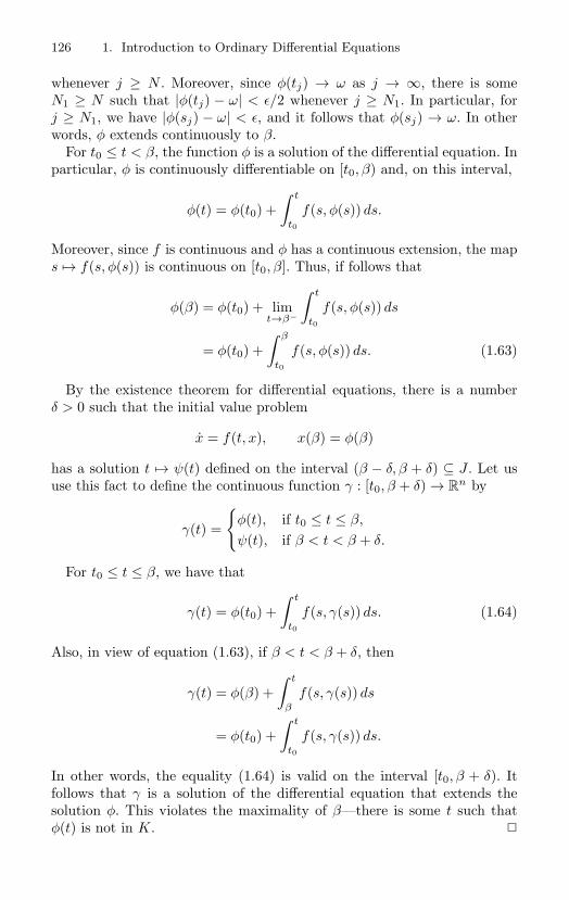
126 1. Introduction to Ordinary Differential Equations
whenever j ≥ N . Moreover, since φ(tj) → ω as j → ∞, there is someN1 ≥ N such that |φ(tj) − ω| < ε/2 whenever j ≥ N1. In particular, forj ≥ N1, we have |φ(sj) − ω| < ε, and it follows that φ(sj) → ω. In otherwords, φ extends continuously to β.
For t0 ≤ t < β, the function φ is a solution of the differential equation. Inparticular, φ is continuously differentiable on [t0, β) and, on this interval,
φ(t) = φ(t0) +∫ t
t0
f(s, φ(s)) ds.
Moreover, since f is continuous and φ has a continuous extension, the maps → f(s, φ(s)) is continuous on [t0, β]. Thus, if follows that
φ(β) = φ(t0) + limt→β−
∫ t
t0
f(s, φ(s)) ds
= φ(t0) +∫ β
t0
f(s, φ(s)) ds. (1.63)
By the existence theorem for differential equations, there is a numberδ > 0 such that the initial value problem
x = f(t, x), x(β) = φ(β)
has a solution t → ψ(t) defined on the interval (β − δ, β + δ) ⊆ J . Let ususe this fact to define the continuous function γ : [t0, β + δ) → R
n by
γ(t) =
φ(t), if t0 ≤ t ≤ β,
ψ(t), if β < t < β + δ.
For t0 ≤ t ≤ β, we have that
γ(t) = φ(t0) +∫ t
t0
f(s, γ(s)) ds. (1.64)
Also, in view of equation (1.63), if β < t < β + δ, then
γ(t) = φ(β) +∫ t
β
f(s, γ(s)) ds
= φ(t0) +∫ t
t0
f(s, γ(s)) ds.
In other words, the equality (1.64) is valid on the interval [t0, β + δ). Itfollows that γ is a solution of the differential equation that extends thesolution φ. This violates the maximality of β—there is some t such thatφ(t) is not in K.
2Linear Systems and Stability
In this chapter we will study the differential equation
x = A(t)x + f(x, t), x ∈ Rn
where A is a smooth n × n matrix-valued function and f is a smoothfunction such that f(0, t) = fx(0, t) ≡ 0. Note that if f has this form, thenthe associated homogeneous linear system x = A(t)x is the linearization ofthe differential equation along the zero solution t → φ(t) ≡ 0.
One of the main objectives of the chapter is the proof of the basic resultsrelated to the principle of linearized stability. For example, we will provethat if the matrix A is constant and all of its eigenvalues have negative realparts, then the zero solution (also called the trivial solution) is asymptoti-cally stable. However, much of the chapter is devoted to the general theoryof homogeneous linear systems; that is, systems of the form x = A(t)x. Inparticular, we will study the important special cases where A is a constantor periodic function.
In case t → A(t) is a constant function, we will show how to reducethe solution of the system x = Ax to a problem in linear algebra. Also, bydefining the matrix exponential, we will discuss the flow of this autonomoussystem as a one-parameter group with generator A.
The nonautonomous system x = A(t)x is not completely understood.However, the solution of the system for the special case where t → A(t) isa periodic matrix-valued function is reducible to the constant matrix case.We will develop a useful theory of periodic matrix systems, called Floquettheory, and use it to prove this basic result. The Floquet theory will ap-pear again later when we discuss the stability of periodic nonhomogeneous
128 2. Linear Systems and Stability
systems. In particular, we will use Floquet theory in a stability analysis ofthe inverted pendulum (see Section 3.5).
Because linear systems theory is so well developed, it is used extensivelyin many areas of applied science. For example, linear systems theory is anessential tool for electromagnetics, circuit theory, and the theory of vibra-tion. In addition, the results of this chapter are a fundamental componentof control theory.
2.1 Homogeneous Linear Differential Equations
This section is devoted to a general discussion of the homogeneous linearsystem
x = A(t)x, x ∈ Rn
where t → A(t) is a smooth function from some open interval J ⊆ R to thespace of n × n matrices. Here, the continuity properties of matrix-valuedfunctions are determined by viewing the space of n × n matrices as R
n2;
that is, every matrix is viewed as an element in the Cartesian space bysimply listing the rows of the matrix consecutively to form a row vector oflength n2. We will prove an important general inequality and then use itto show that solutions of linear systems cannot blow up in finite time. Wewill discuss the basic result that the set of solutions of a linear system is avector space, and we will exploit this fact by showing how to construct thegeneral solution of a linear homogeneous system with constant coefficients.
2.1.1 Gronwall’s InequalityThe important theorem proved in this section does not belong to the theoryof linear differential equations per se, but it is presented here because it willbe used to prove the global existence of solutions of homogeneous linearsystems.
Theorem 2.1 (Gronwall’s Inequality). Suppose that a < b and let α,φ, and ψ be nonnegative continuous functions defined on the interval [a, b].Moreover, suppose that either α is a constant function, or α is differentiableon [a, b] with positive derivative α, If, for all t ∈ [a, b],
φ(t) ≤ α(t) +∫ t
a
ψ(s)φ(s) ds, (2.1)
then
φ(t) ≤ α(t)e∫ t
aψ(s) ds (2.2)
for all t ∈ [a, b].
2.1 Homogeneous Linear Differential Equations 129
Proof. In case α is a constant function, let us assume for the moment thatα > 0. If α is not constant, then, because α > 0 and α is nonnegative, wehave that α is positive on the interval (a, b]. However, let us also assumefor the moment that α(a) > 0.
The function on the interval [a, b] defined by t → α(t) +∫ t
aψ(s)φ(s) ds
is positive and exceeds φ. Thus, we have that
φ(t)
α(t) +∫ t
aψ(s)φ(s) ds
≤ 1.
Multiply both sides of this inequality by ψ(t), add and subtract α(t) in thenumerator of the resulting fraction, rearrange the inequality, and use theobvious estimate to obtain the inequality
α(t) + ψ(t)φ(t)
α(t) +∫ t
aψ(s)φ(s) ds
≤ α(t)α(t)
+ ψ(t),
which, when integrated over the interval [a, t], yields the inequality
ln(α(t) +
∫ t
a
ψ(s)φ(s) ds)
− ln(α(a)) ≤∫ t
a
ψ(s) ds + ln(α(t)) − ln(α(a)).
After we exponentiate both sides of this last inequality and use hypothe-sis (2.1), we find that, for each t in the interval [a, b],
φ(t) ≤ α(t)e∫ t
aψ(s) ds ≤ α(t)e
∫ ta
ψ(s) ds. (2.3)
Finally, if α ≡ 0 or α(a) = 0, then for each ε > 0 we have the inequality
φ(t) ≤ (α(t) + ε) +∫ t
a
ψ(s)φ(s) ds,
and, as a result of what we have just proved, we have the estimate
φ(t) ≤ (α(t) + ε)e∫ t
aψ(s) ds.
The desired inequality follows by passing to the limit (for each fixed t ∈[a, b]) as ε → 0.
Exercise 2.2. What can you say about a continuous function f : R → [0, ∞)if
f(x) ≤∫ x
0f(t) dt?
130 2. Linear Systems and Stability
Exercise 2.3. Prove the “specific Gronwall lemma” [157]: If, for t ∈ [a, b],
φ(t) ≤ δ2(t − a) + δ1
∫ t
a
φ(s) ds + δ3,
where φ is a nonnegative continuous function on [a, b], and δ1 > 0, δ2 ≥ 0, andδ3 ≥ 0 are constants, then
φ(t) ≤(δ2
δ1+ δ3
)eδ1(t−a) − δ2
δ1.
2.1.2 Homogeneous Linear Systems: General TheoryConsider the homogeneous linear system
x = A(t)x, x ∈ Rn. (2.4)
By our general existence theory, the initial value problem
x = A(t)x, x(t0) = x0 (2.5)
has a unique solution that exists on some open interval containing t0. How-ever, for this linear system a stronger statement is true.
Theorem 2.4. If t → A(t) is continuous on the interval α < t < β andif α < t0 < β (maybe α = −∞ or β = ∞), then the solution of the initialvalue problem (2.5) is defined on the open interval (α, β).
Proof. If x0 = 0, then φ(t) ≡ 0 is a solution of the initial value problemthat is defined on the interval (α, β).
Suppose that x0 = 0. Because the continuous function t → A(t) isbounded on each compact subinterval of (α, β), it is easy to see that thefunction (t, x) → A(t)x is locally Lipschitz with respect to its second ar-gument. Consider the solution t → φ(t) of the initial value problem (2.5)given by the general existence theorem (Theorem 1.184) and let J0 denoteits maximal interval of existence. Suppose that J0 does not contain (α, β).For example, suppose that the right hand end point b of J0 is less than β.We will show that this assumption leads to a contradiction. The proof forthe left hand end point is similar.
If t ∈ J0, then we have
φ(t) − φ(t0) =∫ t
t0
A(s)φ(s) ds.
By the continuity of A and the compactness of [t0, b], there is some M > 0such that ‖A(t)‖ ≤ M for all t ∈ [t0, b]. (The notation ‖ ‖ is used for thematrix norm corresponding to some norm ‖ ‖ on R
n.) Thus, for t ∈ J0, we
2.1 Homogeneous Linear Differential Equations 131
have the following inequality:
‖φ(t)‖ ≤ ‖x0‖ +∫ t
t0
‖A(s)‖‖φ(s)‖ ds
≤ ‖x0‖ +∫ t
t0
M‖φ(s)‖ ds.
In addition, by Gronwall’s inequality, with ψ(t) := M , we have
‖φ(t)‖ ≤ ‖x0‖eM
∫ tt0
ds = ‖x0‖eM(t−t0).
Thus, ‖φ(t)‖ is uniformly bounded on [t0, b).By the extensibility theorem and the fact that the boundary of R
n isempty, we must have ‖φ(t)‖ → ∞ as t → b−, in contradiction to theexistence of the uniform bound.
Exercise 2.5. Use Gronwall’s inequality to prove the following important in-equality: If t → β(t) and t → γ(t) are solutions of the smooth differential equationx = f(x) and both are defined on the time interval [0, T ], then there is a constantL > 0 such that
|β(t) − α(t)| ≤ |β(0) − α(0)|eLt.
Thus, two solutions diverge from each other at most exponentially fast. Also,if the solutions have the same initial condition, then they coincide. Therefore,the result of this exercise provides an alternative proof of the general uniquenesstheorem for differential equations.
2.1.3 Principle of SuperpositionThe foundational result about linear homogeneous systems is the principleof superposition: The sum of two solutions is again a solution. A precisestatement of this principle is the content of the next proposition.
Proposition 2.6. If the homogeneous system (2.4) has two solutions φ1(t)and φ2(t), each defined on some interval (a, b), and if λ1 and λ2 are num-bers, then t → λ1φ1(t) + λ2φ2(t) is also a solution defined on the sameinterval.
Proof. To prove the proposition, we use the linearity of the differentialequation. In fact, we have
d
dt(λ1φ1(t) + λ2φ2(t)) = λ1φ1(t) + λ2φ2(t)
= λ1A(t)φ1(t) + λ2A(t)φ2(t)
= A(t)(λ1φ1(t) + λ2φ2(t)).
132 2. Linear Systems and Stability
As a natural extension of the principle of superposition, we will provethat the set of solutions of the homogeneous linear system (2.4) is a finitedimensional vector space of dimension n.
Definition 2.7. A set of n solutions of the homogeneous linear differen-tial equation (2.4), all defined on the same open interval J , is called afundamental set of solutions on J if the solutions are linearly independentfunctions on J .
Proposition 2.8. If t → A(t) is defined on the interval (a, b), then thesystem (2.4) has a fundamental set of solutions defined on (a, b).
Proof. If c ∈ (a, b) and e1, . . . , en denote the usual basis vectors in Rn,
then there is a unique solution t → φi(t) such that φi(c) = ei for i =1, . . . , n. Moreover, by Theorem 2.4, each function φi is defined on theinterval (a, b). Let us assume that the set of functions φi : i = 1, . . . , n islinearly dependent and derive a contradiction. In fact, if there are scalars αi,i = 1, . . . , n, not all zero, such that
∑ni=1 αiφi(t) ≡ 0, then
∑ni=1 αiei ≡ 0.
In view of the linear independence of the usual basis, this is the desiredcontradiction.
Proposition 2.9. If F is a fundamental set of solutions of the linear sys-tem (2.4) on the interval (a, b), then every solution defined on (a, b) can beexpressed as a linear combination of the elements of F .
Proof. Suppose that F = φ1, . . . , φn. Pick c ∈ (a, b). If t → φ(t) isa solution defined on (a, b), then φ(c) and φi(c), for i = 1, . . . , n, are allvectors in R
n. We will show that the set B := φi(c) : i = 1, . . . , nis a basis for R
n. If not, then there are scalars αi, i = 1, . . . , n, not allzero, such that
∑ni=1 αiφi(c) = 0. Thus, y(t) :=
∑ni=1 αiφi(t) is a solution
with initial condition y(c) = 0. But the zero solution has the same initialcondition. Thus, y(t) ≡ 0, and therefore
∑ni=1 αiφi(t) ≡ 0. This contradicts
the hypothesis that F is a linearly independent set, as required.Using the basis B, there are scalars β1, . . . , βn ∈ R such that φ(c) =∑ni=1 βiφi(c). It follows that both φ and
∑ni=1 βiφi are solutions with the
same initial condition, and, by uniqueness, φ =∑n
i=1 βiφi.
Definition 2.10. An n × n matrix function t → Ψ(t), defined on an openinterval J , is called a matrix solution of the homogeneous linear system (2.4)if each of its columns is a (vector) solution. A matrix solution is calleda fundamental matrix solution if its columns form a fundamental set ofsolutions. In addition, a fundamental matrix solution t → Ψ(t) is calledthe principal fundamental matrix at t0 ∈ J if Ψ(t0) = I.
If t → Ψ(t) is a matrix solution of the system (2.4) on the interval J ,then Ψ(t) = A(t)Ψ(t) on J . By Proposition 2.8, there is a fundamentalmatrix solution. Moreover, if t0 ∈ J and t → Φ(t) is a fundamental matrixsolution on J , then (by the linear independence of its columns) the matrix
2.1 Homogeneous Linear Differential Equations 133
Φ(t0) is invertible. It is easy to see that the matrix solution defined byΨ(t) := Φ(t)Φ−1(t0) is the principal fundamental matrix solution at t0.Thus, system (2.4) has a principal fundamental matrix solution at eachpoint in J .
Definition 2.11. The state transition matrix for the homogeneous linearsystem (2.4) on the open interval J is the family of fundamental matrixsolutions t → Ψ(t, τ) parametrized by τ ∈ J such that Ψ(τ, τ) = I, whereI denotes the n × n identity matrix.
Proposition 2.12. If t → Φ(t) is a fundamental matrix solution for thesystem (2.4) on J , then Ψ(t, τ) := Φ(t)Φ−1(τ) is the state transition ma-trix. Also, the state transition matrix satisfies the Chapman–Kolmogorovidentities
Ψ(τ, τ) = I, Ψ(t, s)Ψ(s, τ) = Ψ(t, τ)
and the identities
Ψ(t, s)−1 = Ψ(s, t),∂Ψ∂s
(t, s) = −Ψ(t, s)A(s).
Proof. See Exercise 2.13.
A two-parameter family of operator-valued functions that satisfies theChapman–Kolmogorov identities is called an evolution family.
In the case of constant coefficients, that is, in case t → A(t) is a constantfunction, the corresponding homogeneous linear system is autonomous,and therefore its solutions define a flow. This result also follows from theChapman–Kolmogorov identities.
To prove the flow properties, let us show first that if t → A(t) is aconstant function, then the state transition matrix Ψ(t, t0) depends onlyon the difference t−t0. In fact, since t → Ψ(t, t0) and t → Ψ(t+s, t0+s) areboth solutions satisfying the same initial condition at t0, they are identical.In particular, with s = −t0, we see that Ψ(t, t0) = Ψ(t − t0, 0). If we defineφt := Ψ(t, 0), then using the last identity together with the Chapman–Kolmogorov identities we find that
Ψ(t + s, 0) = Ψ(t, −s) = Ψ(t, 0)Ψ(0,−s) = Ψ(t, 0)Ψ(s, 0).
Thus, we recover the group property φt+s = φtφs. Since, in addition, φ0 =Ψ(0, 0) = I, the family of operators φt defines a flow. In this context, φt isalso called an evolution group.
If t → Φ(t) is a fundamental matrix solution for the linear system (2.4)and v ∈ R
n, then t → Φ(t)v is a (vector) solution. Moreover, every solutionis obtained in this way. In fact, if t → φ(t) is a solution, then there issome v such that Φ(t0)v = φ(t0). (Why?) By uniqueness, we must haveΦ(t)v = φ(t). Also, note that Ψ(t, t0)v has the property that Ψ(t0, t0)v = v.
134 2. Linear Systems and Stability
In other words, Ψ “transfers” the initial state v to the final state Ψ(t, t0)v.Hence, the name “state transition matrix.”
Exercise 2.13. Prove Proposition 2.12.
Exercise 2.14. Suppose u = f(u) is a differential equation on Rn with flow
φt. Show that the family of principal fundamental matrix solutions Φ(t, u) of thefamily of variational equations w = Df(φt(u))w is a linear cocycle over the flowφt; that is, a family of functions, each mapping from R × R
n to the set of lineartransformations of R
n such that Φ(0, u) = I and Φ(t+ s, u) = Φ(t, φs(u))Φ(s, u).(To learn why cocycles are important, see [39].)
The linear independence of a set of solutions of a homogeneous lineardifferential equation can be determined by checking the independence of aset of vectors obtained by evaluating the solutions at just one point. Thisuseful fact is perhaps most clearly expressed by Liouville’s formula.
Proposition 2.15 (Liouville’s formula). Suppose that t → Φ(t) is amatrix solution of the homogeneous linear system (2.4) on the open intervalJ . If t0 ∈ J , then
det Φ(t) = det Φ(t0)e∫ t
t0tr A(s) ds
where det denotes determinant and tr denotes trace. In particular, Φ(t) is afundamental matrix solution if and only if the columns of Φ(t0) are linearlyindependent.
Proof. The matrix solution t → Φ(t) is a differentiable function. Thus, wehave that
limh→0
1h
[Φ(t + h) − (I + hA(t))Φ(t)] = 0.
In other words, using the “little oh” notation,
Φ(t + h) = (I + hA(t))Φ(t) + o(h). (2.6)
(Formally, the little oh has the following meaning: f(x) = g(x)+ o(h(x)) if
limx→0+
|f(x) − g(x)|h(x)
= 0.
Thus, we should write o(±h) in equation (2.6), but this technicality is notimportant in this proof.)
Using the definition of the determinant of an n × n matrix, that is, ifB := (bij), then
det B =∑
σ
sgn(σ)n∏
i=1
bi,σ(i),
2.1 Homogeneous Linear Differential Equations 135
and by the fact that the determinant of a product of matrices is the productof their determinants, we have
det Φ(t + h) = det(I + hA(t)) det Φ(t) + o(h)= (1 + h trA(t)) det Φ(t) + o(h),
and therefored
dtdet Φ(t) = trA(t) det Φ(t).
Integration of this last differential equation gives the desired result.
Exercise 2.16. Find a fundamental matrix solution of the system
x =(
1 −1/t1 + t −1
)x, t > 0.
Hint: x(t) =(
1t
)is a solution.
2.1.4 Linear Equations with Constant CoefficientsIn this section we will consider the homogeneous linear system
x = Ax, x ∈ Rn (2.7)
where A is a real n × n (constant) matrix. We will show how to reducethe problem of constructing a fundamental set of solutions of system (2.7)to a problem in linear algebra. In addition, we will see that the principalfundamental matrix solution at t = 0 is given by the exponential of thematrix tA just as the fundamental scalar solution at t = 0 of the scalardifferential equation x = ax is given by t → eat.
Let us begin with the essential observation of the subject: The solutions ofsystem (2.7) are intimately connected with the eigenvalues and eigenvectorsof the matrix A. To make this statement precise, let us recall that a complexnumber λ is an eigenvalue of A if there is a complex nonzero vector v suchthat Av = λv. In general, the vector v is called an eigenvector associatedwith the eigenvalue λ if Av = λv. Moreover, the set of all eigenvectorsassociated with an eigenvalue forms a vector space. Because a real matrixcan have complex eigenvalues, it is convenient to allow for complex solutionsof the differential equation (2.7). Indeed, if t → u(t) and t → v(t) are realfunctions, and if t → φ(t) is defined by φ(t) := u(t)+ iv(t), then φ is calleda complex solution of system (2.7) provided that u + iv = Au + iAv. Ofcourse, if φ is a complex solution, then we must have u = Au and v = Av.Thus, it is clear that φ is a complex solution if and only if its real andimaginary parts are real solutions. This observation is used in the nextproposition.
136 2. Linear Systems and Stability
Proposition 2.17. Let A be a real n×n matrix and consider the ordinarydifferential equation (2.7).
(1) The function given by t → eλtv is a real solution if and only if λ ∈ R,v ∈ R
n, and Av = λv.
(2) If v = 0 is an eigenvector for A with eigenvalue λ = α + iβ suchthat β = 0, then the imaginary part of v is not zero. In this case, ifv = u + iw ∈ C
n, then there are two real solutions
t → eαt[(cos βt)u − (sin βt)w],
t → eαt[(sinβt)u + (cos βt)w].
Moreover, these solutions are linearly independent.
Proof. If Av = λv, then
d
dt(eλtv) = λeλtv = eλtAv = Aeλtv.
In particular, the function t → eλtv is a solution.If λ = α + iβ and β = 0, then, because A is real, v must be of the form
v = u + iw for some u, w ∈ Rn with w = 0. The real and imaginary parts
of the corresponding solution
eλtv = e(α+iβ)t(u + iw)= eαt(cos βt + i sin βt)(u + iw)= eαt[(cos βt)u − (sin βt)w + i((sinβt)u + (cos βt)w)]
are real solutions of the system (2.7). To show that these real solutionsare linearly independent, suppose that some linear combination of themwith coefficients c1 and c2 is identically zero. Evaluation at t = 0 and att = π/(2β) yields the equations
c1u + c2w = 0, c2u − c1w = 0.
By elimination of u we find that (c21 + c2
2)w = 0. Since w = 0, both coeffi-cients must vanish. This proves (2).
Finally, we will complete the proof of (1). Suppose that λ = α + iβ andv = u+ iv. If eλtv is real, then β = 0 and w = 0. Thus, in fact, λ and v arereal. On the other hand, if λ and v are real, then eλtv is a real solution. Inthis case,
λeλtv = Aeλtv,
and we have that λv = Av.
2.1 Homogeneous Linear Differential Equations 137
A fundamental matrix solution of system (2.7) can be constructed explic-itly if the eigenvalues of A and their multiplicities are known. To illustratethe basic idea, let us suppose that C
n has a basis B := v1, . . . , vn con-sisting of eigenvectors of A, and let λ1, . . . , λn denote the correspondingeigenvalues. For example, if A has n distinct eigenvalues, then the set con-sisting of one eigenvector corresponding to each eigenvalue is a basis of C
n.At any rate, if B is a basis of eigenvectors, then there are n correspondingsolutions given by
t → eλitvi, i = 1, . . . , n,
and the matrix
Φ(t) = [eλ1tv1, . . . eλntvn],
which is partitioned by columns, is a matrix solution. Because det Φ(0) =0, this solution is a fundamental matrix solution, and moreover Ψ(t) :=Φ(t)Φ−1(0) is the principal fundamental matrix solution of (2.7) at t =0. Let us note that a principal fundamental matrix for a real system isnecessarily real. In fact, if Λ(t) denotes the imaginary part of a principalfundamental matrix solution, then Λ(0) = 0. But then, by the uniquenessof solutions of initial value problems, Λ(t) ≡ 0. Thus, even if some of theeigenvalues of A are complex, the fundamental matrix solution t → Φ(t)defined above is real.
Continuing under the assumption that A has a basis B of eigenvectors,let us show that there is a change of coordinates that transforms the systemx = Ax, x ∈ R
n, to a decoupled system of n scalar differential equations.To prove this result, let us first define the matrix B := [v1, . . . , vn] whosecolumns are the eigenvectors in B. The matrix B is invertible. Indeed,consider the action of B on the usual basis vectors and recall that the vectorobtained by multiplication of a vector by a matrix is a linear combination ofthe columns of the matrix; that is, if w = (w1, . . . , wn) is (the transpose of)a vector in C
n, then the product Bw is equal to∑n
i=1 wivi. In particular,we have Bei = vi, i = 1, . . . , n. This proves that B is invertible. In fact,B−1 is the unique linear map such that B−1vi = ei.
Using the same idea, let us compute
B−1AB = B−1A[v1, . . . , vn]
= B−1[λ1v1, . . . , λnvn]
= [λ1e1, . . . , λnen]
=
λ1 0. . .
0 λn
.
In other words, D := B−1AB is a diagonal matrix with the eigenvaluesof A as its diagonal elements. The diffeomorphism of C
n given by the
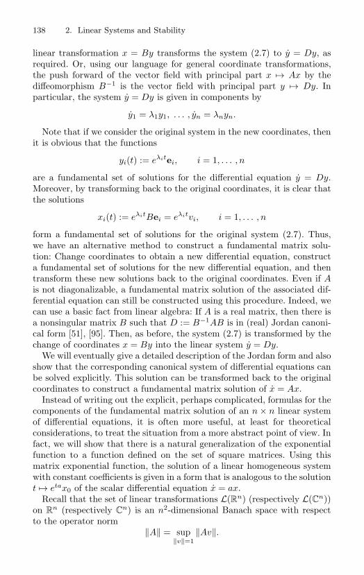
138 2. Linear Systems and Stability
linear transformation x = By transforms the system (2.7) to y = Dy, asrequired. Or, using our language for general coordinate transformations,the push forward of the vector field with principal part x → Ax by thediffeomorphism B−1 is the vector field with principal part y → Dy. Inparticular, the system y = Dy is given in components by
y1 = λ1y1, . . . , yn = λnyn.
Note that if we consider the original system in the new coordinates, thenit is obvious that the functions
yi(t) := eλitei, i = 1, . . . , n
are a fundamental set of solutions for the differential equation y = Dy.Moreover, by transforming back to the original coordinates, it is clear thatthe solutions
xi(t) := eλitBei = eλitvi, i = 1, . . . , n
form a fundamental set of solutions for the original system (2.7). Thus,we have an alternative method to construct a fundamental matrix solu-tion: Change coordinates to obtain a new differential equation, constructa fundamental set of solutions for the new differential equation, and thentransform these new solutions back to the original coordinates. Even if Ais not diagonalizable, a fundamental matrix solution of the associated dif-ferential equation can still be constructed using this procedure. Indeed, wecan use a basic fact from linear algebra: If A is a real matrix, then there isa nonsingular matrix B such that D := B−1AB is in (real) Jordan canoni-cal form [51], [95]. Then, as before, the system (2.7) is transformed by thechange of coordinates x = By into the linear system y = Dy.
We will eventually give a detailed description of the Jordan form and alsoshow that the corresponding canonical system of differential equations canbe solved explicitly. This solution can be transformed back to the originalcoordinates to construct a fundamental matrix solution of x = Ax.
Instead of writing out the explicit, perhaps complicated, formulas for thecomponents of the fundamental matrix solution of an n × n linear systemof differential equations, it is often more useful, at least for theoreticalconsiderations, to treat the situation from a more abstract point of view. Infact, we will show that there is a natural generalization of the exponentialfunction to a function defined on the set of square matrices. Using thismatrix exponential function, the solution of a linear homogeneous systemwith constant coefficients is given in a form that is analogous to the solutiont → etax0 of the scalar differential equation x = ax.
Recall that the set of linear transformations L(Rn) (respectively L(Cn))on R
n (respectively Cn) is an n2-dimensional Banach space with respect
to the operator norm‖A‖ = sup
‖v‖=1‖Av‖.
2.1 Homogeneous Linear Differential Equations 139
Most of the theory we will develop is equally valid for either of the vectorspaces R
n or Cn. When the space is not at issue, we will denote the Banach
space of linear transformations by L(E) where E may be taken as eitherR
n or Cn. The theory is also valid for the set of (operator norm) bounded
linear transformations of an arbitrary Banach space.
Exercise 2.18. Prove: L(E) is a finite dimensional Banach space with respectto the operator norm.
Exercise 2.19. The space of n×n matrices is a topological space with respectto the operator topology. Prove that the set of matrices with n distinct eigenvaluesis open and dense. A property that is defined on the countable intersection ofopen dense sets is called generic.
Proposition 2.20. If A ∈ L(E), then the series I +∑∞
n=11n!A
n is abso-lutely convergent.
Proof. It suffices to show that the sequence of partial sums SN∞N=1 for
the series 1 +∑∞
n=11n!‖An‖ is a Cauchy sequence. Let us define
SN := 1 + ‖A‖ +12!
‖A2‖ + · · · +1
N !‖AN‖.
Note that the partial sums of the convergent series
∞∑n=0
‖A‖n
n!= e‖A‖
form a Cauchy sequence. Using this fact, the estimate ‖An‖ ≤ ‖A‖n, andthe triangle inequality, it follows that SN is a Cauchy sequence in L(E).
Define the exponential map exp : L(E) → L(E) by
exp(A) := I +∞∑
n=1
1n!
An.
Also, let us use the notation eA := exp(A).The main properties of the exponential map are summarized in the fol-
lowing proposition.
Proposition 2.21. Suppose that A, B ∈ L(E).
(0) If A ∈ L(Rn), then eA ∈ L(Rn).
(1) If B is nonsingular, then B−1eAB = eB−1AB.
(2) If AB = BA, then eA+B = eAeB.
140 2. Linear Systems and Stability
(3) e−A = (eA)−1. In particular, the image of exp is in the general lineargroup GL(E) consisting of the invertible elements of L(E).
(4) ddt (e
tA) = AetA = etAA. In particular, t → etA is the fundamentalmatrix solution of the system (2.7) at t = 0.
(5) ‖eA‖ ≤ e‖A‖.
Proof. The proof of (0) is obvious.To prove (1), define
SN := I + A +12!
A2 + · · · +1
N !AN ,
and note that if B is nonsingular, then B−1AnB = (B−1AB)n. Thus, wehave that
B−1SNB = I + B−1AB +12!
(B−1AB)2 + · · · +1
N !(B−1AB)N ,
and, by the definition of the exponential map,
limN→∞
B−1SNB = eB−1AB .
Using the continuity of the linear map on L(E) defined by C → B−1CB,it follows that
limN→∞
B−1SNB = B−1eAB,
as required.As the first step in the proof of (4), consider the following proposition: If
s, t ∈ R, then e(s+t)A = esAetA. To prove it, let us denote the partial sumsfor the series representation of etA by
SN (t) := I + tA +12!
(tA)2 + · · · +1
N !(tA)N
= I + tA +12!
t2A2 + · · · +1
N !tNAN .
We claim that
SN (s)SN (t) = SN (s + t) +2N∑
n=N+1
Pn(s, t)An (2.8)
where Pn(s, t) is a homogeneous polynomial of degree n such that
|Pn(s, t)| ≤ (|s| + |t|)n
n!.
2.1 Homogeneous Linear Differential Equations 141
To obtain this identity, note that the nth order term of the product, atleast for 0 ≤ n ≤ N , is given by( n∑
j=0
1(n − j)!j!
sn−jtj)An =
( 1n!
n∑j=0
n!(n − j)!j!
sn−jtj)An =
1n!
(s + t)nAn.
Also, for N + 1 ≤ n ≤ 2N , the nth order term is essentially the same, onlysome of the summands are missing. In fact, these terms all have the form( n∑
j=0
δ(j)(n − j)!j!
sn−jtj)An
where δ(j) has value zero or one. Each such term is the product of An
and a homogeneous polynomial in two variables of degree n. Moreover, therequired estimate for the polynomial follows from the fact that |δ(j)| ≤ 1.This proves the claim.
Using equation (2.8), we have the following inequality
‖SN (s)SN (t) − SN (s + t)‖ ≤2N∑
n=N+1
|Pn(s, t)| ‖A‖n
≤2N∑
n=N+1
(|s| + |t|)n
n!‖A‖n.
Also, using the fact that the series∞∑
n=0
(|s| + |t|)n
n!‖A‖n
is convergent, it follows that its partial sums, denoted QN , form a Cauchysequence. In particular, if ε > 0 is given, then for sufficiently large N wehave
|Q2N − QN | < ε.
Moreover, since
Q2N − QN =2N∑
n=N+1
(|s| + |t|)n
n!‖A‖n,
it follows thatlim
N→∞‖SN (s)SN (t) − SN (s + t)‖ = 0.
Using this fact and passing to the limit as N → ∞ on both sides of theinequality
‖esAetA − e(s+t)A‖ ≤ ‖esAetA − SN (s)SN (t)‖
+ ‖SN (s)SN (t) − SN (s + t)‖
+ ‖SN (s + t) − e(s+t)A‖,
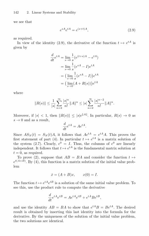
142 2. Linear Systems and Stability
we see that
esAetA = e(s+t)A, (2.9)
as required.In view of the identity (2.9), the derivative of the function t → etA is
given by
d
dtetA = lim
s→0
1s(e(t+s)A − etA)
= lims→0
1s(esA − I)etA
=(
lims→0
1s(esA − I)
)etA
=(
lims→0
(A + R(s)))etA
where
‖R(s)‖ ≤ 1|s|
∞∑n=2
|s|nn!
‖A‖n ≤ |s|∞∑
n=2
|s|n−2
n!‖A‖n.
Moreover, if |s| < 1, then ‖R(s)‖ ≤ |s|e‖A‖. In particular, R(s) → 0 ass → 0 and as a result,
d
dtetA = AetA.
Since ASN (t) = SN (t)A, it follows that AetA = etAA. This proves thefirst statement of part (4). In particular t → etA is a matrix solution ofthe system (2.7). Clearly, e0 = I. Thus, the columns of e0 are linearlyindependent. It follows that t → etA is the fundamental matrix solution att = 0, as required.
To prove (2), suppose that AB = BA and consider the function t →et(A+B). By (4), this function is a matrix solution of the initial value prob-lem
x = (A + B)x, x(0) = I.
The function t → etAetB is a solution of the same initial value problem. Tosee this, use the product rule to compute the derivative
d
dtetAetB = AetAetB + etABetB ,
and use the identity AB = BA to show that etAB = BetA. The desiredresult is obtained by inserting this last identity into the formula for thederivative. By the uniqueness of the solution of the initial value problem,the two solutions are identical.
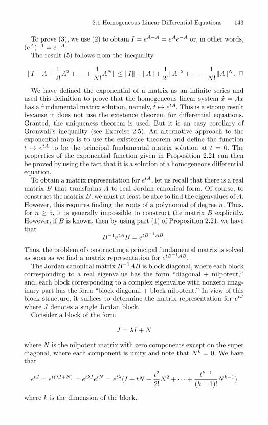
2.1 Homogeneous Linear Differential Equations 143
To prove (3), we use (2) to obtain I = eA−A = eAe−A or, in other words,(eA)−1 = e−A.
The result (5) follows from the inequality
‖I +A+12!
A2 + · · ·+ 1N !
AN‖ ≤ ‖I‖+ ‖A‖+12!
‖A‖2 + · · ·+ 1N !
‖A‖N .
We have defined the exponential of a matrix as an infinite series andused this definition to prove that the homogeneous linear system x = Axhas a fundamental matrix solution, namely, t → etA. This is a strong resultbecause it does not use the existence theorem for differential equations.Granted, the uniqueness theorem is used. But it is an easy corollary ofGronwall’s inequality (see Exercise 2.5). An alternative approach to theexponential map is to use the existence theorem and define the functiont → etA to be the principal fundamental matrix solution at t = 0. Theproperties of the exponential function given in Proposition 2.21 can thenbe proved by using the fact that it is a solution of a homogeneous differentialequation.
To obtain a matrix representation for etA, let us recall that there is a realmatrix B that transforms A to real Jordan canonical form. Of course, toconstruct the matrix B, we must at least be able to find the eigenvalues of A.However, this requires finding the roots of a polynomial of degree n. Thus,for n ≥ 5, it is generally impossible to construct the matrix B explicitly.However, if B is known, then by using part (1) of Proposition 2.21, we havethat
B−1etAB = etB−1AB .
Thus, the problem of constructing a principal fundamental matrix is solvedas soon as we find a matrix representation for etB−1AB .
The Jordan canonical matrix B−1AB is block diagonal, where each blockcorresponding to a real eigenvalue has the form “diagonal + nilpotent,”and, each block corresponding to a complex eigenvalue with nonzero imag-inary part has the form “block diagonal + block nilpotent.” In view of thisblock structure, it suffices to determine the matrix representation for etJ
where J denotes a single Jordan block.Consider a block of the form
J = λI + N
where N is the nilpotent matrix with zero components except on the superdiagonal, where each component is unity and note that Nk = 0. We havethat
etJ = et(λI+N) = etλIetN = etλ(I + tN +t2
2!N2 + · · · +
tk−1
(k − 1)!Nk−1)
where k is the dimension of the block.
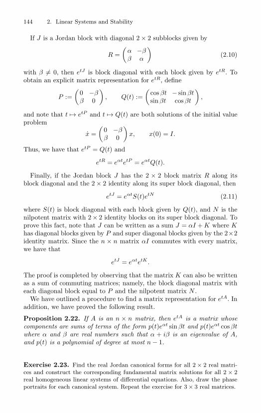
144 2. Linear Systems and Stability
If J is a Jordan block with diagonal 2 × 2 subblocks given by
R =(
α −ββ α
)(2.10)
with β = 0, then etJ is block diagonal with each block given by etR. Toobtain an explicit matrix representation for etR, define
P :=(
0 −ββ 0
), Q(t) :=
(cos βt − sin βtsin βt cos βt
),
and note that t → etP and t → Q(t) are both solutions of the initial valueproblem
x =(
0 −ββ 0
)x, x(0) = I.
Thus, we have that etP = Q(t) and
etR = eαtetP = eαtQ(t).
Finally, if the Jordan block J has the 2 × 2 block matrix R along itsblock diagonal and the 2 × 2 identity along its super block diagonal, then
etJ = eαtS(t)etN (2.11)
where S(t) is block diagonal with each block given by Q(t), and N is thenilpotent matrix with 2 × 2 identity blocks on its super block diagonal. Toprove this fact, note that J can be written as a sum J = αI + K where Khas diagonal blocks given by P and super diagonal blocks given by the 2×2identity matrix. Since the n × n matrix αI commutes with every matrix,we have that
etJ = eαtetK .
The proof is completed by observing that the matrix K can also be writtenas a sum of commuting matrices; namely, the block diagonal matrix witheach diagonal block equal to P and the nilpotent matrix N .
We have outlined a procedure to find a matrix representation for etA. Inaddition, we have proved the following result.
Proposition 2.22. If A is an n × n matrix, then etA is a matrix whosecomponents are sums of terms of the form p(t)eαt sin βt and p(t)eαt cos βtwhere α and β are real numbers such that α + iβ is an eigenvalue of A,and p(t) is a polynomial of degree at most n − 1.
Exercise 2.23. Find the real Jordan canonical forms for all 2 × 2 real matri-ces and construct the corresponding fundamental matrix solutions for all 2 × 2real homogeneous linear systems of differential equations. Also, draw the phaseportraits for each canonical system. Repeat the exercise for 3 × 3 real matrices.
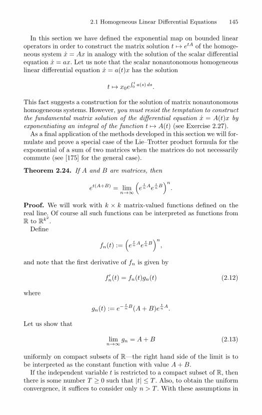
2.1 Homogeneous Linear Differential Equations 145
In this section we have defined the exponential map on bounded linearoperators in order to construct the matrix solution t → etA of the homoge-neous system x = Ax in analogy with the solution of the scalar differentialequation x = ax. Let us note that the scalar nonautonomous homogeneouslinear differential equation x = a(t)x has the solution
t → x0e∫ t0 a(s) ds.
This fact suggests a construction for the solution of matrix nonautonomoushomogeneous systems. However, you must resist the temptation to constructthe fundamental matrix solution of the differential equation x = A(t)x byexponentiating an integral of the function t → A(t) (see Exercise 2.27).
As a final application of the methods developed in this section we will for-mulate and prove a special case of the Lie–Trotter product formula for theexponential of a sum of two matrices when the matrices do not necessarilycommute (see [175] for the general case).
Theorem 2.24. If A and B are matrices, then
et(A+B) = limn→∞
(e
tn Ae
tn B
)n
.
Proof. We will work with k × k matrix-valued functions defined on thereal line. Of course all such functions can be interpreted as functions fromR to R
k2.
Define
fn(t) :=(e
tn Ae
tn B
)n
,
and note that the first derivative of fn is given by
f ′n(t) = fn(t)gn(t) (2.12)
where
gn(t) := e− tn B(A + B)e
tn A.
Let us show that
limn→∞ gn = A + B (2.13)
uniformly on compact subsets of R—the right hand side of the limit is tobe interpreted as the constant function with value A + B.
If the independent variable t is restricted to a compact subset of R, thenthere is some number T ≥ 0 such that |t| ≤ T . Also, to obtain the uniformconvergence, it suffices to consider only n > T . With these assumptions in
146 2. Linear Systems and Stability
force, consider the estimate
‖e− tn B(A + B)e
tn A − (A + B)‖
≤ e|t|n ‖B‖‖(A + B)e
tn B − (A + B) + (A + B) − e
tn B(A + B)‖
≤ e|T |n ‖B‖(‖A + B‖‖e
tn B − I‖ + ‖I − e
tn B‖‖A + B‖
)and note that
‖etn B − I‖ ≤ T
ne‖B‖.
The uniform convergence follows immediately because T/n can be madearbitrarily small by taking n sufficiently large.
We will use the limit (2.13) to show that the sequence of functionsfn∞
n=1 converges uniformly on compact sets.Let us show first that the required convergence is uniform on the interval
[0, T ]. To prove this fact, integrate both sides of equation (2.12) to obtainthe equality
fn(t) = I +∫ t
0fn(s)gn(s) ds,
and, in turn, the estimate
‖fm(t) − fn(t)‖ =∫ t
0‖fm(s)gm(s) − fm(s)gn(s)
+fm(s)gn(s) − fn(s)gn(s)‖ ds
≤∫ t
0‖fm(s)‖‖gm(s) − gn(s)‖ ds
+∫ t
0‖fm(s) − fn(s)‖‖gn(s)‖ ds. (2.14)
Because the sequence of functions gn∞n=1 converges uniformly on [0, T ], it
is uniformly bounded. Also, by using the definition of fn and the propertiesof the norm, we have the uniform bound
‖fn(t)‖ ≤ eT‖A‖eT‖B‖.
Hence, there is a constant M ≥ 0 such that, for the uniform (supremum)norm on the interval [0, T ], we have the inequalities ‖fn‖ ≤ M and ‖gn‖ ≤M for each positive integer n. Moreover, since the sequence of functionsgn∞
n=1 converges uniformly on [0, T ], there is some integer N > 0 suchthat
‖gm − gn‖ < ε
2.1 Homogeneous Linear Differential Equations 147
whenever n ≥ N and m ≥ M .Let ε > 0 be given. Using the inequality (2.14) and the uniform estimates
given in the last paragraph, it follows that
‖fm(t) − fn(t)‖ ≤ Mεt + M
∫ t
0‖fm(s) − fn(s)‖ ds,
and, by Gronwall’s inequality,
‖fm − fn‖ ≤ εMTeMT .
Thus, we have proved that fn∞n=1 is a Cauchy sequence in the uniform
norm on the interval [0, T ].For the required uniform convergence on the interval [−T, 0], apply the
result just obtained to the sequence of functions hn∞n=1 defined by
hn(t) := fn(−t) =(e
tn (−A)e
tn (−B)
)n
.
Because fn∞n=1 is a Cauchy sequence in the uniform norm, there is a
continuous function f , defined on the interval [−T, T ], such that
limn→∞ fn = f.
Also, the sequence gn∞n=1 converges to the constant function with value
A + B. Using these facts together with the identity f ′n(t) = fn(t)gn(t),
let us note that the sequence f ′n∞
n=1 converges uniformly to the functiondefined by t → f(t)(A + B). Thus, the function f is differentiable, f ′(t) =f(t)(A + B) (see the proof of Theorem 1.176), and f(0) = I. The solutionof this initial value problem is
f(t) = et(A+B),
that is, the limit function f is as required in the statement of the theorem.
Exercise 2.25. Compute the fundamental matrix solution at t = 0 for thesystem x = Ax where
A :=
1 2 3
0 1 40 0 1
.
Exercise 2.26. Determine the phase portrait for the system(xy
)=
(0 1
−1 −k
) (xy
).
Make sure you distinguish the cases k < −2, k > 2, k = 0, 0 < k < 2, and−2 < k < 0.
148 2. Linear Systems and Stability
Exercise 2.27. Find a matrix function t → A(t) such that
t → exp( ∫ t
0A(s) ds
)
is not a matrix solution of the system x = A(t)x. However, show that the givenexponential formula is a solution in the scalar case. When is it a solution for thematrix case?
Exercise 2.28. [Lie Groups and Lax Pairs] Is the map
exp : L(E) → GL(E)
injective? Is this map surjective? Do the answers to these questions depend onthe choice of E as R
n or Cn? Prove that the general linear group is a submanifold
of RN with N = n2 in case E = R
n, and N = 2n2 in case E = Cn. Show that the
general linear group is a Lie group; that is, the group operation (matrix product),is a differentiable map from GL(E) × GL(E) → GL(E). Consider the tangentspace at the identity element of GL(E). Note that, for each A ∈ L(E), the mapt → exp(tA) is a curve in GL(E) passing through the origin at time t = 0. Usethis fact to prove that the tangent space can be identified with L(E). It turns outthat L(E) is a Lie algebra. More generally, a vector space is called a Lie algebraif for each pair of vectors A and B, a product, denoted by [A, B], is defined onthe vector space such that the product is bilinear and also satisfies the followingalgebraic identities: (skew-symmetry) [A, B] = −[B, A], and (the Jacobi identity)
[[A, B], C] + [[B, C], A] + [[C, A], B] = 0.
Show that L(E) is a Lie algebra with respect to the product [A, B] := AB −BA.For an elementary introduction to the properties of these structures, see [91].
The delicate interplay between Lie groups and Lie algebras leads to a far-reaching theory. To give a flavor of the relationship between these structures,consider the map Ad : GL(E) → L(L(E)) defined by Ad(A)(B) = ABA−1. Thismap defines the adjoint representation of the Lie group into the automorphismsof the Lie algebra. Prove this. Also, Ad is a homomorphism of groups: Ad(AB) =Ad(A) Ad(B). Note that we may as well denote the automorphism group of L(E)by GL(L(E)). Also, define ad : L(E) → L(L(E)) by ad(A)(B) = [A, B]. The mapad is a homomorphism of Lie algebras. Now, ϕt := Ad(etA) defines a flow in L(E).The associated differential equation is obtained by differentiation. Show that ϕt
is the flow of the differential equation
x = Ax − xA = ad(A)x. (2.15)
This differential equation is linear; thus, it has the solution t → et ad(A). By theusual argument it now follows that et ad(A) = Ad(etA). In particular, we have thecommutative diagram
L(E) ad−→ L(L(E))expexp
GL(E) Ad−→ GL(L(E)).
2.1 Homogeneous Linear Differential Equations 149
The adjoint representation of GL(E) is useful in the study of the subgroups ofGL(E), and it is also used to identify the Lie group that is associated with a givenLie algebra. But consider instead the following application to spectral theory. Acurve t → L(t) in L(E) is called isospectral if the spectrum of L(t) is the same asthe spectrum of L(0) for all t ∈ R. We have the following proposition: Supposethat A ∈ L(E). If t → L(t) is a solution of the differential equation (2.15), thenthe solution is isospectral. The proof is just a restatement of the content of thecommutative diagram. In fact, L(t) is similar to L(0) because
L(t) = Ad(etA)L(0) = etAL(0)e−tA.
A pair of curves t → L(t) and t → M(t) is called a Lax pair if
L = LM − ML.
The sign convention aside, the above proposition shows that if (L, M) is a Laxpair and if M is constant, then L is isospectral. Prove the more general result: If(L, M) is a Lax pair, then L is isospectral.
Finally, prove that
d
dt
(etAetBe−tAe−tB)∣∣∣
t=0= 0
and
d
dt
(e
√tAe
√tBe−√
tAe−√tB)∣∣∣
t=0= AB − BA. (2.16)
As mentioned above, [A, B] is in the tangent space at the identity of GL(E).Thus, there is a curve γ(t) in GL(E) such that γ(0) = I and γ(0) = [A, B]. Onesuch curve is t → et[A,B]. However, since the Lie bracket [A, B] is an algebraicobject computed from the tangent vectors A and B, it is satisfying that there isanother such curve formed from the curves t → etA and t → etB whose respectivetangent vectors at t = 0 are A and B.
Exercise 2.29. Prove that if α is a real number and A is an n × n real matrixsuch that 〈Av, v〉 ≤ α‖v‖2 for all v ∈ R
n, then ‖etA‖ ≤ eαt for all t ≥ 0. Hint:Consider the differential equation x = Ax and the inner product 〈x, x〉. Prove thefollowing more general result suggested by Weishi Liu. Suppose that t → A(t)and t → B(t) are smooth n × n matrix valued functions defined on R such that〈A(t)v, v〉 ≤ α(t)‖v‖2 and 〈B(t)v, v〉 ≤ 0 for all t ≥ 0 and all v ∈ R
n. If t → x(t)is a solution of the differential equation x = A(t)x + B(t)x, then
‖x(t)‖ ≤ e∫ t0 α(s) ds‖x(0)‖
for all t ≥ 0.
Exercise 2.30. Let v ∈ R3, assume v = 0, and consider the differential equa-
tion
x = v × x, x(0) = x0
150 2. Linear Systems and Stability
where × denotes the cross product in R3. Show that the solution of the differential
equation is a rigid rotation of the initial vector x0 about the direction v. If thedifferential equation is written as a matrix system
x = Sx
where S is a 3 × 3 matrix, show that S is skew symmetric and that the flowφt(x) = etSx of the system is a group of orthogonal transformations. Show thatevery solution of the system is periodic and relate the period to the length of v.
Exercise 2.31. [An infinite dimensional ODE] Let E denote the Banach spaceC([0, 1]) given by the set of all continuous functions f : [0, 1] → R with thesupremum norm
‖f‖ = sups∈[0,1]
|f(s)|
and consider the operator U : E → E given by (Uf)(s) = f(as) where 0 ≤ a ≤ 1.Also, let g ∈ E denote the function given by s → bs where b is a fixed realnumber. Find the solution of the initial value problem
x = Ux, x(0) = g.
This is a simple example of an ordinary differential equation on an infinite di-mensional Banach space (see Section 3.6).
Exercise 2.32. Prove the following generalization of the Lie-Trotter productformula. If γ : R → L(E) is a smooth function and A := γ(0), then
etA = limn→∞
(γ(t/n))n.
The Lie-Trotter formula is recovered by inserting γ(t) = etAetB . For exam-ple, et[A,B] can be approximated using the generalized product formula and for-mula (2.16).
Exercise 2.33. Write a report on the application of the Lie-Trotter formulato obtain numerical approximations of the solution of the initial value problemx = (A + B)x, x(0) = v with expressions of the form
T (t, n)v = (e(t/n)Ae(t/n)B)nv.
For example, approximate x(1) for such systems where
A :=(
a 00 b
), B :=
(c −dd c
).
Compare the results of numerical experiments using your implementation(s) ofthe “Lie-Trotter method” and your favorite choice of alternative method(s) tocompute x(1). Note that etA and etB can be input explicitly for the suggestedexample. Can you estimate the error ‖T (1, n)v − eA+Bv‖? Generalizations ofthis scheme are sometimes used to approximate differential equations where the“vector field” can be split into two easily solved summands. Try the same ideato solve nonlinear ODE of the form x = f(x) + g(x) where etA is replaced by theflow of x = f(x) and etB is replaced by the flow of x = g(x).
2.2 Stability of Linear Systems 151
2.2 Stability of Linear Systems
A linear homogeneous differential equation has a rest point at the origin. Wewill use our results about the solutions of constant coefficient homogeneouslinear differential equations to study the stability of this rest point. Thenext result is fundamental.
Theorem 2.34. Suppose that A is an n × n (real) matrix. The followingstatements are equivalent:
(1) There is a norm | |a on Rn and a real number λ > 0 such that for
all v ∈ Rn and all t ≥ 0,
|etAv|a ≤ e−λt|v|a.
(2) If | |g denotes a norm on Rn, there is a constant C ≥ 1 and a real
number λ > 0 such that for all v ∈ Rn and all t ≥ 0,
|etAv|g ≤ Ce−λt|v|g.
(3) Every eigenvalue of A has negative real part.
Moreover, if −λ exceeds the largest of all the real parts of the eigenvalues ofA, then λ can be taken to be the decay constant in (1) or (2). Also, if everyeigenvalue of A has negative real part, then the zero solution of x = Ax isasymptotically stable.
Proof. We will show that (1) ⇒ (2) ⇒ (3) ⇒ (1).To show (1) ⇒ (2), let | |a be the norm in statement (1) and | |g
the norm in statement (2). Because these norms are defined on the finitedimensional vector space R
n, they are equivalent. In particular, there areconstants K1 > 0 and K2 > 0 such that for all x ∈ R
n we have
K1|x|g ≤ |x|a ≤ K2|x|g.
(Prove this!)If t ≥ 0 and x ∈ R
n, then
|etAx|g ≤ 1K1
|etAx|a ≤ 1K1
e−λt|x|a ≤ K2
K1e−λt|x|g,
as required.To show (2) ⇒ (3), suppose that statement (2) holds but statement (3)
does not. In particular, A has an eigenvalue µ ∈ C, say µ = α + iβ withα ≥ 0. Moreover, there is at least one eigenvector v = 0 corresponding tothis eigenvalue. As we have seen, this implies that x = Ax has a solutiont → γ(t) of the form t → eαt((cos βt)u − (sin βt)w) where v = u + iw,u ∈ R
n and w ∈ Rn. As α ≥ 0 and at least one of the vectors u and v is
152 2. Linear Systems and Stability
not zero, it is clear that limt→∞ γ(t) = 0. But if statement (2) holds, thenlimt→∞ γ(t) = 0, in contradiction.
To finish the proof we will show (3) ⇒ (1). Let us assume that state-ment (3) holds. Since A has a finite set of eigenvalues and each of itseigenvalues has negative real part, there is a number λ > 0 such that thereal part of each eigenvalue of A is less than −λ.
By Proposition 2.22, the components of etA are sums of terms of the formp(t)eαt sin βt or p(t)eαt cos βt where α is the real part of an eigenvalue ofA and p(t) is a polynomial of degree at most n − 1. In particular, if thematrix etA, partitioned by columns, is given by [c1(t), . . . , cn(t)], then eachcomponent of each vector ci(t) is a sum of such terms.
If v = (v1, . . . , vn) is a vector in Rn, then with respect to the usual norm
of Rn we have
|etAv| ≤n∑
i=1
|ci(t)||vi|.
Because
|vi| ≤( n∑
i=1
|vi|2)1/2 = |v|,
it follows that
|etAv| ≤ |v|n∑
i=1
|ci(t)|.
If β1, . . . , β are the nonzero imaginary parts of the eigenvalues of A andif α denotes the largest real part of an eigenvalue of A, then using thestructure of the components of the vector ci(t) it follows that
|ci(t)|2 ≤ e2αt2n−2∑k=0
|dki(t)||t|k
where each coefficient dki(t) is a quadratic form in
sin β1t, . . . , sin βt, cos β1t, . . . , cos βt.
There is a constant M > 0 that does not depend on i or k such that thesupremum of |dki(t)| for t ∈ R does not exceed M2. In particular, for eachi = 1, . . . , n, we have
|ci(t)|2 ≤ e2αtM22n−2∑k=0
|t|k,
and as a result
|etAv| ≤ |v|n∑
i=1
|ci(t)| ≤ eαtnM |v|( 2n−2∑
k=0
|t|k)1/2
.
2.2 Stability of Linear Systems 153
Because α < −λ < 0, there is some τ > 0 such that for t ≥ τ , we havethe inequality
e(λ+α)tnM( 2n−2∑
k=0
|t|k)1/2 ≤ 1,
or equivalently
eαtnM( 2n−2∑
k=0
|t|k)1/2 ≤ e−λt.
In particular, if t ≥ τ , then for each v ∈ Rn we have
|etAv| ≤ e−λt|v|. (2.17)
To finish the proof, we will construct a new norm for which the sameinequality is valid for all t ≥ 0. In fact, we will prove that
|v|a :=∫ τ
0eλs|esAv| ds
is the required norm.The easy proof required to show that | |a is a norm on R
n is left tothe reader. To obtain the norm estimate, note that for each t ≥ 0 thereis a nonnegative integer m and a number T such that 0 ≤ T < τ andt = mτ + T . Using this decomposition of t, we find that
|etAv|a =∫ τ
0eλs|esAetAv| ds
=∫ τ−T
0eλs|e(s+t)Av| ds +
∫ τ
τ−T
eλs|e(s+t)A| ds
=∫ τ−T
0eλs|emτAe(s+T )Av| ds
+∫ τ
τ−T
eλs|e(m+1)τAe(T−τ+s)Av| ds.
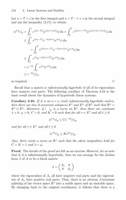
154 2. Linear Systems and Stability
Let u = T + s in the first integral and u = T − τ + s in the second integraland use the inequality (2.17), to obtain
|etAv|a =∫ τ
T
eλ(u−T )|e(mτ+u)Av| du +∫ T
0eλ(u+τ−T )|e((m+1)τ+u)Av| du
≤∫ τ
T
eλ(u−T )e−λ(mτ)|euAv| du
+∫ T
0eλ(u+τ−T )e−λ(m+1)τ |euAv| du
≤∫ τ
0eλue−λ(mτ+T )|euAv| du
= e−λt
∫ τ
0eλu|euAv| du
≤ e−λt|v|a,
as required.
Recall that a matrix is infinitesimally hyperbolic if all of its eigenvalueshave nonzero real parts. The following corollary of Theorem 2.34 is thebasic result about the dynamics of hyperbolic linear systems.
Corollary 2.35. If A is an n × n (real) infinitesimally hyperbolic matrix,then there are two A-invariant subspaces Es and Eu of R
n such that Rn =
Es ⊕ Eu. Moreover, if | |g is a norm on Rn, then there are constants
λ > 0, µ > 0, C > 0, and K > 0 such that for all v ∈ Es and all t ≥ 0
|etAv|g ≤ Ce−λt|v|g,
and for all v ∈ Eu and all t ≤ 0
|etAv|g ≤ Keµt|v|g.
Also, there exists a norm on Rn such that the above inequalities hold for
C = K = 1 and λ = µ.
Proof. The details of the proof are left as an exercise. However, let us notethat if A is infinitesimally hyperbolic, then we can arrange for the Jordanform J of A to be a block matrix
J =(
As 00 Au
)where the eigenvalues of As all have negative real parts and the eigenval-ues of Au have positive real parts. Thus, there is an obvious J-invariantsplitting of the vector space R
n into a stable space and an unstable space.By changing back to the original coordinates, it follows that there is a
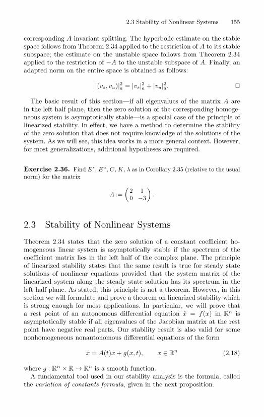
2.3 Stability of Nonlinear Systems 155
corresponding A-invariant splitting. The hyperbolic estimate on the stablespace follows from Theorem 2.34 applied to the restriction of A to its stablesubspace; the estimate on the unstable space follows from Theorem 2.34applied to the restriction of −A to the unstable subspace of A. Finally, anadapted norm on the entire space is obtained as follows:
|(vs, vu)|2a = |vs|2a + |vu|2a.
The basic result of this section—if all eigenvalues of the matrix A arein the left half plane, then the zero solution of the corresponding homoge-neous system is asymptotically stable—is a special case of the principle oflinearized stability. In effect, we have a method to determine the stabilityof the zero solution that does not require knowledge of the solutions of thesystem. As we will see, this idea works in a more general context. However,for most generalizations, additional hypotheses are required.
Exercise 2.36. Find Es, Eu, C, K, λ as in Corollary 2.35 (relative to the usualnorm) for the matrix
A :=(
2 10 −3
).
2.3 Stability of Nonlinear Systems
Theorem 2.34 states that the zero solution of a constant coefficient ho-mogeneous linear system is asymptotically stable if the spectrum of thecoefficient matrix lies in the left half of the complex plane. The principleof linearized stability states that the same result is true for steady statesolutions of nonlinear equations provided that the system matrix of thelinearized system along the steady state solution has its spectrum in theleft half plane. As stated, this principle is not a theorem. However, in thissection we will formulate and prove a theorem on linearized stability whichis strong enough for most applications. In particular, we will prove thata rest point of an autonomous differential equation x = f(x) in R
n isasymptotically stable if all eigenvalues of the Jacobian matrix at the restpoint have negative real parts. Our stability result is also valid for somenonhomogeneous nonautonomous differential equations of the form
x = A(t)x + g(x, t), x ∈ Rn (2.18)
where g : Rn × R → R
n is a smooth function.A fundamental tool used in our stability analysis is the formula, called
the variation of constants formula, given in the next proposition.
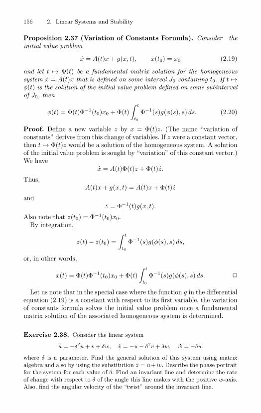
156 2. Linear Systems and Stability
Proposition 2.37 (Variation of Constants Formula). Consider theinitial value problem
x = A(t)x + g(x, t), x(t0) = x0 (2.19)
and let t → Φ(t) be a fundamental matrix solution for the homogeneoussystem x = A(t)x that is defined on some interval J0 containing t0. If t →φ(t) is the solution of the initial value problem defined on some subintervalof J0, then
φ(t) = Φ(t)Φ−1(t0)x0 + Φ(t)∫ t
t0
Φ−1(s)g(φ(s), s) ds. (2.20)
Proof. Define a new variable z by x = Φ(t)z. (The name “variation ofconstants” derives from this change of variables. If z were a constant vector,then t → Φ(t)z would be a solution of the homogeneous system. A solutionof the initial value problem is sought by “variation” of this constant vector.)We have
x = A(t)Φ(t)z + Φ(t)z.
Thus,A(t)x + g(x, t) = A(t)x + Φ(t)z
andz = Φ−1(t)g(x, t).
Also note that z(t0) = Φ−1(t0)x0.By integration,
z(t) − z(t0) =∫ t
t0
Φ−1(s)g(φ(s), s) ds,
or, in other words,
x(t) = Φ(t)Φ−1(t0)x0 + Φ(t)∫ t
t0
Φ−1(s)g(φ(s), s) ds.
Let us note that in the special case where the function g in the differentialequation (2.19) is a constant with respect to its first variable, the variationof constants formula solves the initial value problem once a fundamentalmatrix solution of the associated homogeneous system is determined.
Exercise 2.38. Consider the linear system
u = −δ2u + v + δw, v = −u − δ2v + δw, w = −δw
where δ is a parameter. Find the general solution of this system using matrixalgebra and also by using the substitution z = u+ iv. Describe the phase portraitfor the system for each value of δ. Find an invariant line and determine the rateof change with respect to δ of the angle this line makes with the positive w-axis.Also, find the angular velocity of the “twist” around the invariant line.
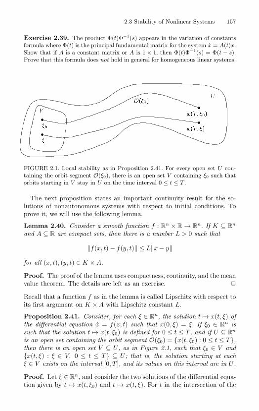
2.3 Stability of Nonlinear Systems 157
Exercise 2.39. The product Φ(t)Φ−1(s) appears in the variation of constantsformula where Φ(t) is the principal fundamental matrix for the system x = A(t)x.Show that if A is a constant matrix or A is 1 × 1, then Φ(t)Φ−1(s) = Φ(t − s).Prove that this formula does not hold in general for homogeneous linear systems.
xT
O
V
U
xT
FIGURE 2.1. Local stability as in Proposition 2.41. For every open set U con-taining the orbit segment O(ξ0), there is an open set V containing ξ0 such thatorbits starting in V stay in U on the time interval 0 ≤ t ≤ T .
The next proposition states an important continuity result for the so-lutions of nonautonomous systems with respect to initial conditions. Toprove it, we will use the following lemma.
Lemma 2.40. Consider a smooth function f : Rn × R → R
n. If K ⊆ Rn
and A ⊆ R are compact sets, then there is a number L > 0 such that
‖f(x, t) − f(y, t)‖ ≤ L‖x − y‖
for all (x, t), (y, t) ∈ K × A.
Proof. The proof of the lemma uses compactness, continuity, and the meanvalue theorem. The details are left as an exercise.
Recall that a function f as in the lemma is called Lipschitz with respect toits first argument on K × A with Lipschitz constant L.
Proposition 2.41. Consider, for each ξ ∈ Rn, the solution t → x(t, ξ) of
the differential equation x = f(x, t) such that x(0, ξ) = ξ. If ξ0 ∈ Rn is
such that the solution t → x(t, ξ0) is defined for 0 ≤ t ≤ T , and if U ⊆ Rn
is an open set containing the orbit segment O(ξ0) = x(t, ξ0) : 0 ≤ t ≤ T,then there is an open set V ⊆ U , as in Figure 2.1, such that ξ0 ∈ V andx(t, ξ) : ξ ∈ V, 0 ≤ t ≤ T ⊆ U ; that is, the solution starting at eachξ ∈ V exists on the interval [0, T ], and its values on this interval are in U .
Proof. Let ξ ∈ Rn, and consider the two solutions of the differential equa-
tion given by t → x(t, ξ0) and t → x(t, ξ). For t in the intersection of the
158 2. Linear Systems and Stability
intervals of existence of these solutions, we have that
x(t, ξ) − x(t, ξ0) = ξ − ξ0 +∫ t
0f(x(s, ξ), s) − f(x(s, ξ0), s) ds
and
‖x(t, ξ) − x(t, ξ0)‖ ≤ ‖ξ − ξ0‖ +∫ t
0‖f(x(s, ξ), s) − f(x(s, ξ0), s)‖ ds.
We can assume without loss of generality that U is bounded, hence itsclosure is compact. It follows from the lemma that the smooth function fis Lipschitz on U × [0, T ] with a Lipschitz constant L > 0. Thus, as long as(x(t, ξ), t) ∈ U × [0, T ], we have
‖x(t, ξ) − x(t, ξ0)‖ ≤ ‖ξ − ξ0‖ +∫ t
0L‖x(s, ξ) − x(s, ξ0)‖ ds
and by Gronwall’s inequality
‖x(t, ξ) − x(t, ξ0)‖ ≤ ‖ξ − ξ0‖eLt.
Let δ > 0 be such that δeLT is less than the distance from O(ξ0) to theboundary of U . Since, on the intersection J of the domain of definition ofthe solution t → x(t, ξ) with [0, T ] we have
‖x(t, ξ) − x(t, ξ0)‖ ≤ ‖ξ − ξ0‖eLT ,
the vector x(t, ξ) is in the bounded set U as long as t ∈ J and ‖ξ − ξ0‖ < δ.By the extensibility theorem, the solution t → x(t, ξ) is defined at least onthe interval [0, T ]. Thus, the desired set V is ξ ∈ U : ‖ξ − ξ0‖ < δ.
We are now ready to formulate a theoretical foundation for Lyapunov’sindirect method, that is, the method of linearization. The idea should befamiliar: If the system has a rest point at the origin, the linearization ofthe system has an asymptotically stable rest point at the origin, and thenonlinear part is appropriately bounded, then the nonlinear system alsohas an asymptotically stable rest point at the origin.
Theorem 2.42. Consider the initial value problem (2.19) for the casewhere A := A(t) is a (real) matrix of constants. If all eigenvalues of Ahave negative real parts and there are positive constants a > 0 and k > 0such that ‖g(x, t)‖ ≤ k‖x‖2 whenever ‖x‖ < a, then there are positive con-stants C, b, and α that are independent of the choice of the initial time t0such that the solution t → x(t) of the initial value problem satisfies
‖x(t)‖ ≤ C‖x0‖e−α(t−t0) (2.21)
for t ≥ t0 whenever ‖x0‖ ≤ b. In particular, the function t → x(t) isdefined for all t ≥ t0, and the zero solution (the solution with initial valuex(t0) = 0), is asymptotically stable.
2.3 Stability of Nonlinear Systems 159
Proof. By Theorem 2.34 and the hypothesis on the eigenvalues of A, thereare constants C > 1 and λ > 0 such that
‖etA‖ ≤ Ce−λt (2.22)
for t ≥ 0. Fix δ > 0 such that δ < a and Ckδ − λ < 0, define α := λ − Ckδand b := δ/C, and note that α > 0 and 0 < b < δ < a.
If ‖x0‖ < b, then there is some half open interval J = t ∈ R : t0 ≤ t < τsuch that the solution t → x(t) of the differential equation with initialcondition x(t0) = x0 exists and satisfies the inequality
‖x(t)‖ < δ (2.23)
on the interval J .For t ∈ J , use the estimate
‖g(x(t), t)‖ ≤ kδ‖x(t)‖,
the estimate (2.22), and the variation of constants formula
x(t) = e(t−t0)Ax0 + e(t−t0)A∫ t
t0
e(t0−s)Ag(x(s), s) ds
to obtain the inequality
‖x(t)‖ ≤ Ce−λ(t−t0)‖x0‖ +∫ t
t0
Ce−λ(t−s)kδ‖x(s)‖ ds.
Rearrange the inequality to the form
eλ(t−t0)‖x(t)‖ ≤ C‖x0‖ + Ckδ
∫ t
t0
eλ(s−t0)‖x(s)‖ ds
and apply Gronwall’s inequality to obtain the estimate
eλ(t−t0)‖x(t)‖ ≤ C‖x0‖eCkδ(t−t0);
or equivalently
‖x(t)‖ ≤ C‖x0‖e(Ckδ−λ)(t−t0) ≤ C‖x0‖e−α(t−t0). (2.24)
Thus, if ‖x0‖ < b and ‖x(t)‖ < δ for t ∈ J , then the required inequal-ity (2.21) is satisfied for t ∈ J .
If J is not the interval [t0,∞), then the set of all numbers τ > t0 suchthat the solution t → x(t) with initial condition x(t0) = x0 is defined fort0 ≤ t < τ and ‖x(t)‖ < δ has a finite supremum that we again denote byτ . In this case, because ‖x0‖ < δ/C and in view of the inequality (2.24),we have that
‖x(t)‖ < δe−α(t−t0) (2.25)
160 2. Linear Systems and Stability
for t0 ≤ t < τ . In particular, the solution is bounded by δ on the inter-val [t0, τ). Therefore, by the extensibility theorem there is some numberε > 0 such that the solution is defined on the interval K := [t0, τ + ε).Using the fact that the function t → ‖x(t)‖ is continuous on K and theinequality (2.25), it follows that
‖x(τ)‖ < δe−α(τ−t0) < δ.
By using this inequality and again using the continuity of the functiont → ‖x(t)‖ on K, there is a number η > 0 such that t → x(t) is defined onthe interval [t0, τ + η), and, on this interval, ‖x(t)‖ < δ. This contradictsthe fact that τ is maximal.
Corollary 2.43. If f : Rn → R
n is smooth, f(ξ) = 0, and and all eigen-values of Df(ξ) have negative real parts, then the differential equationx = f(x) has an asymptotically stable rest point at ξ. Moreover, if −αis a number larger than every real part of an eigenvalue of Df(x0), and φt
is the flow of the differential equation, then there is a neighborhood U of ξand a constant C > 0 such that
‖φt(x) − ξ‖ ≤ C‖x‖e−αt
whenever x ∈ U and t ≥ 0.
Proof. It suffices to prove the corollary for the case ξ = 0. By Taylor’stheorem (Theorem 1.168), we can rewrite the differential equation in theform x = Df(0)x + g(x) where
g(x) :=∫ 1
0(Df(sx) − Df(0))x ds.
The function ξ → Df(ξ) is smooth. Thus, by the mean value theorem(Theorem 1.49),
‖Df(sx) − Df(0)‖ ≤ ‖sx‖ supτ∈[0,1]
‖D2f(τsx)‖
≤ ‖x‖ supτ∈[0,1]
‖D2f(τx)‖.
Again, by the smoothness of f , there is an open ball B centered at theorigin and a constant k > 0 such that
supτ∈[0,1]
‖D2f(τx)‖ < k
for all x ∈ B. Moreover, by an application of Proposition 1.166 and theabove estimates we have that
‖g(x)‖ ≤ sups∈[0,1]
‖x‖‖Df(sx) − Df(0)‖ ≤ k‖x‖2
2.3 Stability of Nonlinear Systems 161
whenever x ∈ B. The desired result now follows directly from Theorem 2.42.
Exercise 2.44. Generalize the previous result to the Poincare–Lyapunov The-orem: Let
x = Ax + B(t)x + g(x, t), x(t0) = x0, x ∈ Rn
be a smooth initial value problem. If
(1) A is a constant matrix with spectrum in the left half plane,
(2) B(t) is the n×n matrix, continuously dependent on t such that ‖B(t)‖ → 0as t → ∞,
(3) g(x, t) is smooth and there are constants a > 0 and k > 0 such that
‖g(x, t)‖ ≤ k‖x‖2
for all t ≥ 0 and ‖x‖ < a,
then there are constants C > 1, δ > 0, λ > 0 such that
‖x(t)‖ ≤ C‖x0‖e−λ(t−t0), t ≥ t0
whenever ‖x0‖ ≤ δ/C. In particular, the zero solution is asymptotically stable.
Exercise 2.45. This exercise gives an alternative proof of the principle of lin-earized stability for autonomous systems using Lyapunov’s direct method. Con-sider the system
x = Ax + g(x), x ∈ Rn
where A is a real n × n matrix and g : Rn → R
n is a smooth function. Supposethat every eigenvalue of A has negative real part, and that for some a > 0, thereis a constant k > 0 such that, using the usual norm in R
n,
|g(x)| ≤ k|x|2
whenever |x| < a. Prove that the origin is an asymptotically stable rest point byconstructing a quadratic Lyapunov function. For this, let 〈·, ·〉 denote the usualinner product on R
n, and let A∗ denote the transpose of the real matrix A.Suppose that there is a real symmetric positive definite n × n matrix that alsosatisfies Lyapunov’s equation
A∗B + BA = −I
and define V : Rn → R by
V (x) = 〈x, Bx〉.Show that the restriction of V to a sufficiently small neighborhood of the origin isa strict Lyapunov function. To do this, you will have to estimate a certain innerproduct using the Schwarz inequality. Also, show that
B :=∫ ∞
0etA∗
etA dt
162 2. Linear Systems and Stability
is a symmetric positive definite n × n matrix that satisfies Lyapunov’s equation.Use the fact that A∗ and A have the same eigenvalues together with the exponen-tial estimates for a hyperbolic matrix to prove that the integral converges. Notethat Lyapunov’s equation gives a purely algebraic way to construct a Lyapunovfunction from the system matrix A. Finally, prove that the origin is asymptoti-cally stable for the system x = Ax + g(x) where
A :=
−1 2 0
−2 −1 00 0 −3
, g(u, v, w) :=
u2 + uv + v2 + wv2
w2 + uvww3
.
Exercise 2.46. Suppose that f : Rn → R
n is conservative; that is, there issome function g : R
n → R and f(x) = grad g(x). Also, suppose that M and ∆are symmetric positive definite n×n matrices. Consider the differential equation
Mx + ∆x + f(x) = 0, x ∈ Rn
and note that, in case M and ∆ are diagonal, the differential equation can beviewed as a model of n particles each moving according to Newton’s secondlaw in a conservative force field with viscous damping. Prove that the functionV : R
n → R defined by
V (x, y) :=12〈My, y〉 +
∫ 1
0〈f(tx), x〉 dt
decreases along orbits of the associated first order system
x = y, My = −∆y − f(x);
in fact, V = −〈∆y, y〉. Conclude that the system has no periodic orbits. Also,prove that if f(0) = 0 and Df(0) is positive definite, then the system has anasymptotically stable rest point at the origin. Prove this fact in two ways: usingthe function V and by the method of linearization.
2.4 Floquet Theory
In this section, we will begin the study of linear systems of the form
x = A(t)x, x ∈ Rn (2.26)
where t → A(t) is a T -periodic continuous matrix-valued function. Themain theorem in this section, Floquet’s theorem, gives a canonical form foreach fundamental matrix solution. This result will be used to show thatthere is a periodic time-dependent change of coordinates that transformssystem (2.26) into a homogeneous linear system with constant coefficients.
Floquet’s theorem is a corollary of the following result about the rangeof the exponential map.
2.4 Floquet Theory 163
Theorem 2.47. If C is a nonsingular n×n matrix, then there is an n×nmatrix B, possibly complex, such that eB = C. If C is a nonsingular realn × n matrix, then there is a real n × n matrix B such that eB = C2.
Proof. If S is a nonsingular n × n matrix such that S−1CS = J is inJordan canonical form, and if eK = J , then SeKS−1 = C. As a result,eSKS−1
= C and B = SKS−1 is the desired matrix. Thus, it suffices toconsider the nonsingular matrix C or C2 to be a Jordan block.
For the first statement of the theorem, assume that C = λI + N whereN is nilpotent; that is, Nm = 0 for some integer m with 0 ≤ m < n.Because C is nonsingular, λ = 0 and we can write C = λ(I + (1/λ)N). Acomputation using the series representation of the function t → ln(1 + t)at t = 0 shows that, formally (that is, without regard to the convergenceof the series), if B = (lnλ)I + M where
M =m−1∑j=1
(−1)j+1
jλjN j ,
then eB = C. But because N is nilpotent, the series are finite. Thus, theformal series identity is an identity. This proves the first statement of thetheorem.
If C is real, note that the real eigenvalues of C2 are all positive. Considerin turn four types of real Jordan blocks: rI where r > 0; rI + N wherer > 0 and N is real nilpotent; block diagonal with 2 × 2 subblocks of theform R as in equation (2.10) corresponding to eigenvalues with nonzeroimaginary parts; and “block diagonal plus block nilpotent.” Because thereal eigenvalues are positive, a real “logarithm” for the first two types ofblocks is obtained by the matrix formula given above. For the third blocktype, write
R = r
(cos θ − sin θsin θ cos θ
)where r > 0, and note that a real logarithm is given by
ln rI +(
0 −θθ 0
).
Finally, for a “block diagonal plus block nilpotent” Jordan block, factorthe Jordan block as follows:
R(I + N )
where R is block diagonal with R along the diagonal and N has 2 × 2blocks on its super diagonal all given by R−1. Note that we have alreadyobtained logarithms for each of these factors. Moreover, it is not difficultto check that the two logarithms commute. Thus, a real logarithm of theJordan block is obtained as the sum of real logarithms of the factors.
164 2. Linear Systems and Stability
Theorem 2.48 (Floquet’s Theorem). If Φ(t) is a fundamental matrixsolution of the T -periodic system (2.26), then, for all t ∈ R,
Φ(t + T ) = Φ(t)Φ−1(0)Φ(T ).
In addition, for each possibly complex matrix B such that
eTB = Φ−1(0)Φ(T ),
there is a possibly complex T -periodic matrix function t → P (t) such thatΦ(t) = P (t)etB for all t ∈ R. Also, there is a real matrix R and a real2T -periodic matrix function t → Q(t) such that Φ(t) = Q(t)etR for allt ∈ R.
Proof. Since the function t → A(t) is periodic, it is defined for all t ∈ R.Thus, by Theorem 2.4, all solutions of the system are defined for t ∈ R.
If Ψ(t) := Φ(t + T ), then Ψ is a matrix solution. Indeed, we have that
Ψ(t) = Φ(t + T ) = A(t + T )Φ(t + T ) = A(t)Ψ(t),
as required.Define
C := Φ−1(0)Φ(T ) = Φ−1(0)Ψ(0),
and note that C is nonsingular. The matrix function t → Φ(t)C is clearlya matrix solution of the linear system with initial value Φ(0)C = Ψ(0). Bythe uniqueness of solutions, Ψ(t) = Φ(t)C for all t ∈ R. In particular, wehave that
Φ(t + T ) = Φ(t)C = Φ(t)Φ−1(0)Φ(T ),Φ(t + 2T ) = Φ((t + T ) + T ) = Φ(t + T )C = Φ(t)C2.
By Theorem 2.47, there is a matrix B, possibly complex, such that
eTB = C.
Also, there is a real matrix R such that
e2TR = C2.
If P (t) := Φ(t)e−tB and Q(t) := Φ(t)e−tR, then
P (t + T ) = Φ(t + T )e−TBe−tB = Φ(t)Ce−TBe−tB = Φ(t)e−tB = P (t),
Q(t + 2T ) = Φ(t + 2T )e−2TRe−tR = Φ(t)e−tR = Q(t).
Thus, we have P (t + T ) = P (t), Q(t + 2T ) = Q(t), and
Φ(t) = P (t)etB = Q(t)etR,
as required.
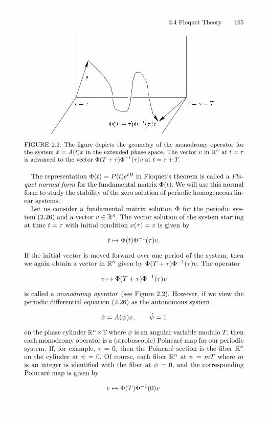
2.4 Floquet Theory 165
T v
v
t t T
FIGURE 2.2. The figure depicts the geometry of the monodromy operator forthe system x = A(t)x in the extended phase space. The vector v in R
n at t = τis advanced to the vector Φ(T + τ)Φ−1(τ)v at t = τ + T .
The representation Φ(t) = P (t)etB in Floquet’s theorem is called a Flo-quet normal form for the fundamental matrix Φ(t). We will use this normalform to study the stability of the zero solution of periodic homogeneous lin-ear systems.
Let us consider a fundamental matrix solution Φ for the periodic sys-tem (2.26) and a vector v ∈ R
n. The vector solution of the system startingat time t = τ with initial condition x(τ) = v is given by
t → Φ(t)Φ−1(τ)v.
If the initial vector is moved forward over one period of the system, thenwe again obtain a vector in R
n given by Φ(T + τ)Φ−1(τ)v. The operator
v → Φ(T + τ)Φ−1(τ)v
is called a monodromy operator (see Figure 2.2). However, if we view theperiodic differential equation (2.26) as the autonomous system
x = A(ψ)x, ψ = 1
on the phase cylinder Rn×T where ψ is an angular variable modulo T , then
each monodromy operator is a (stroboscopic) Poincare map for our periodicsystem. If, for example, τ = 0, then the Poincare section is the fiber R
n
on the cylinder at ψ = 0. Of course, each fiber Rn at ψ = mT where m
is an integer is identified with the fiber at ψ = 0, and the correspondingPoincare map is given by
v → Φ(T )Φ−1(0)v.
166 2. Linear Systems and Stability
The eigenvalues of a monodromy operator are called characteristic multi-pliers of the corresponding time-periodic homogeneous system (2.26). Thenext proposition states that characteristic multipliers are nonzero complexnumbers that are intrinsic to the periodic system—they do not depend onthe choice of the fundamental matrix or the initial time.
Proposition 2.49. The following statements are valid for the periodic lin-ear homogeneous system (2.26).
(1) Every monodromy operator is invertible. In particular, every charac-teristic multiplier is nonzero.
(2) If M1 and M2 are monodromy operators, then they have the sameeigenvalues. In particular, there are exactly n characteristic multipli-ers, counting multiplicities.
Proof. The first statement of the proposition is obvious from the defini-tions.
To prove statement (2), let us consider the principal fundamental matrixΦ(t) at t = 0. If Ψ(t) is a fundamental matrix, then Ψ(t) = Φ(t)Ψ(0). Also,by Floquet’s theorem,
Φ(t + T ) = Φ(t)Φ−1(0)Φ(T ).
Consider the monodromy operator M given by
v → Ψ(T + τ)Ψ−1(τ)v
and note that
Ψ(T + τ)Ψ−1(τ) = Φ(T + τ)Ψ(0)Ψ−1(0)Φ−1(τ)= Φ(T + τ)Φ−1(τ)= Φ(τ)Φ−1(0)Φ(T )Φ−1(τ)= Φ(τ)Φ(T )Φ−1(τ).
In particular, the eigenvalues of the operator Φ(T ) are the same as theeigenvalues of the monodromy operator M. Thus, all monodromy operatorshave the same eigenvalues.
Because
Φ(t + T ) = Φ(t)Φ−1(0)Φ(T ),
some authors define characteristic multipliers to be the eigenvalues of thematrices defined by Φ−1(0)Φ(T ) where Φ(t) is a fundamental matrix. How-ever, both definitions gives the same characteristic multipliers. To prove thisfact, let us consider the Floquet normal form Φ(t) = P (t)etB and note thatΦ(0) = P (0) = P (T ). Thus, we have that
Φ−1(0)Φ(T ) = eTB .
2.4 Floquet Theory 167
Also, by using the Floquet normal form,
Φ(T )Φ−1(0) = P (T )eTBΦ−1(0)= Φ(0)eTBΦ−1(0)= Φ(0)(Φ−1(0)Φ(T ))Φ−1(0),
and therefore Φ−1(0)Φ(T ) has the same eigenvalues as the monodromyoperator given by
v → Φ(T )Φ−1(0)v.
In particular, the traditional definition agrees with our geometrically mo-tivated definition.
Returning to the Floquet normal form P (t)etB for the fundamental ma-trix Φ(t) and the monodromy operator
v → Φ(T + τ)Φ−1(τ)v,
we have that
Φ(T + τ)Φ−1(τ) = P (τ)eTBP−1(τ).
Thus, the characteristic multipliers of the system are the eigenvalues of eTB .The complex number µ is called a characteristic exponent (or a Floquetexponent) of the system, if ρ is a characteristic multiplier and eµT = ρ.Note that if eµT = ρ, then µ + 2πik/T is also a Floquet exponent foreach integer k. Thus, although the characteristic multipliers are uniquelydefined, the Floquet exponents are not.
Exercise 2.50. Suppose that a : R → R is a T -periodic function. Find thecharacteristic multiplier and a Floquet exponent of the T -periodic system x =a(t)x. Also, find the Floquet normal form for the principal fundamental matrixsolution of this system at t = t0.
Exercise 2.51. For the autonomous linear system x = Ax a fundamental ma-trix solution t → Φ(t) satisfies the identity Φ(T − t) = Φ(T )Φ−1(t). Show that,in general, this identity does not hold for nonautonomous homogeneous linearsystems. Hint: Write down a Floquet normal form matrix Φ(t) = P (t)etB thatdoes not satisfy the identity and then show that it is the solution of a (periodic)nonautonomous homogeneous linear system.
Let us suppose that a fundamental matrix for the system (2.26) is repre-sented in Floquet normal form by P (t)etB . We have seen that the charac-teristic multipliers of the system are the eigenvalues of eTB . However, thedefinition of the Floquet exponents does not mention the eigenvalues ofB. Are the eigenvalues of B Floquet exponents? This question is answeredaffirmatively by the following general theorem about the exponential map.
168 2. Linear Systems and Stability
Theorem 2.52. If A is an n×n matrix and if λ1, . . . , λn are the eigenval-ues of A repeated according to their algebraic multiplicity, then λk
1 , . . . , λkn
are the eigenvalues of Ak and eλ1 , . . . , eλn are the eigenvalues of eA.
Proof. We will prove the theorem by induction on the dimension n.The theorem is clearly valid for 1 × 1 matrices. Suppose that it is true
for all (n − 1) × (n − 1) matrices. Define λ := λ1, and let v = 0 denote acorresponding eigenvector so that Av = λv. Also, let e1, . . . , en denote theusual basis of C
n. There is a nonsingular n×n matrix S such that Sv = e1.(Why?) Thus,
SAS−1e1 = λe1,
and it follows that the matrix SAS−1 has the block form
SAS−1 =(
λ ∗0 A
).
The matrix SAkS−1 has the same block form, only with the block di-agonal elements λk and Ak. Clearly the eigenvalues of this block matrixare λk together with the eigenvalues of Ak. By induction, the eigenvaluesof Ak are the kth powers of the eigenvalues of A. This proves the secondstatement of the theorem.
Using the power series definition of exp, we see that eSAS−1has block
form, with block diagonal elements eλ and eA. Clearly, the eigenvalues ofthis block matrix are eλ together with the eigenvalues of eA. Again usinginduction, it follows that the eigenvalues of eA are eλ2 , . . . , eλn . Thus, theeigenvalues of eSAS−1
= SeAS−1 are eλ1 , . . . , eλn .
Theorem 2.52 is an example of a spectral mapping theorem. If we letσ(A) denote the spectrum of the matrix A, that is, the set of all λ ∈ C suchthat λI − A is not invertible, then, for our finite dimensional matrix, σ(A)coincides with the set of eigenvalues of A. Theorem 2.52 can be restated asfollows: eσ(A) = σ(eA).
The next result uses Floquet theory to show that the differential equa-tion (2.26) is equivalent to a homogeneous linear system with constantcoefficients. This result demonstrates that the stability of the zero solutioncan often be determined by the Floquet multipliers.
Theorem 2.53. There is a time-dependent (2T -periodic) change of coor-dinates, x = Q(t)y, that transforms the periodic system (2.26) to a (real)constant coefficient linear system.
(1) If the characteristic multipliers of the periodic system (2.26) all havemodulus less than one; equivalently, if all characteristic exponentshave negative real part, then the zero solution is asymptotically stable.
(2) If the characteristic multipliers of the periodic system (2.26) all havemodulus less than or equal to one; equivalently, if all characteristic
2.4 Floquet Theory 169
exponents have nonpositive real part, and if the algebraic multiplic-ity equals the geometric multiplicity of each characteristic multiplierwith modulus one; equivalently, if the algebraic multiplicity equals thegeometric multiplicity of each characteristic exponent with real partzero, then the zero solution is Lyapunov stable.
(3) If at least one characteristic multiplier of the periodic system (2.26)has modulus greater than one; equivalently, if a characteristic expo-nent has positive real part, then the zero solution is unstable.
Proof. We will prove the first statement of the theorem and part (1). Theproof of the remaining two parts is left as an exercise. However, for part (2),note that since the differential equation is linear, the Lyapunov stabilitymay reasonably be determined from the eigenvalues of a linearization.
There is a real matrix R and a real 2T -periodic matrix Q(t) such thatthe principal fundamental matrix solution Φ(t) of the system is representedby
Φ(t) = Q(t)etR.
Also, there is a matrix B and a T -periodic matrix P such that
Φ(t) = P (t)etB .
The characteristic multipliers are the eigenvalues of eTB . Using the factthat Φ(0) is the identity matrix, we have that
Φ(2T ) = e2TR = e2TB ,
and in particular(eTB)2 = e2TR.
By Theorem 2.52, the eigenvalues of e2TR are the squares of the character-istic multipliers. These all have modulus less than one. Thus, by anotherapplication of Theorem 2.52, all eigenvalues of the real matrix R have neg-ative real parts.
Let us use the change of variables x = Q(t)y to compute
A(t)x = Q(t)y + Q(t)y,
or equivalentlyQ(t)y = (A(t)Q(t) − Q(t))y
andy = Q−1(t)(A(t)Q(t) − Q(t))y.
Also, let us use the Floquet representation Q(t) = Φ(t)e−tR to compute
Q(t) = A(t)Φ(t)e−tR + Φ(t)e−tR(−R)= A(t)Q(t) − Q(t)R.
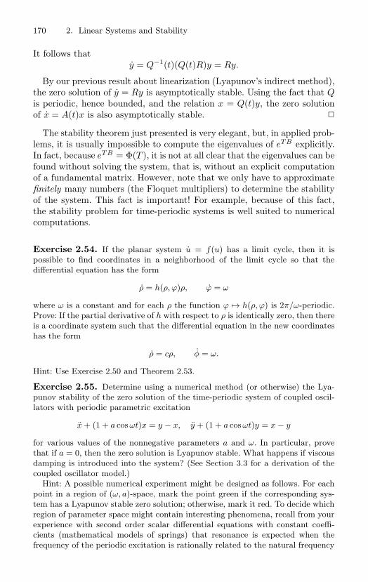
170 2. Linear Systems and Stability
It follows thaty = Q−1(t)(Q(t)R)y = Ry.
By our previous result about linearization (Lyapunov’s indirect method),the zero solution of y = Ry is asymptotically stable. Using the fact that Qis periodic, hence bounded, and the relation x = Q(t)y, the zero solutionof x = A(t)x is also asymptotically stable.
The stability theorem just presented is very elegant, but, in applied prob-lems, it is usually impossible to compute the eigenvalues of eTB explicitly.In fact, because eTB = Φ(T ), it is not at all clear that the eigenvalues can befound without solving the system, that is, without an explicit computationof a fundamental matrix. However, note that we only have to approximatefinitely many numbers (the Floquet multipliers) to determine the stabilityof the system. This fact is important! For example, because of this fact,the stability problem for time-periodic systems is well suited to numericalcomputations.
Exercise 2.54. If the planar system u = f(u) has a limit cycle, then it ispossible to find coordinates in a neighborhood of the limit cycle so that thedifferential equation has the form
ρ = h(ρ, ϕ)ρ, ϕ = ω
where ω is a constant and for each ρ the function ϕ → h(ρ, ϕ) is 2π/ω-periodic.Prove: If the partial derivative of h with respect to ρ is identically zero, then thereis a coordinate system such that the differential equation in the new coordinateshas the form
ρ = cρ, φ = ω.
Hint: Use Exercise 2.50 and Theorem 2.53.
Exercise 2.55. Determine using a numerical method (or otherwise) the Lya-punov stability of the zero solution of the time-periodic system of coupled oscil-lators with periodic parametric excitation
x + (1 + a cos ωt)x = y − x, y + (1 + a cos ωt)y = x − y
for various values of the nonnegative parameters a and ω. In particular, provethat if a = 0, then the zero solution is Lyapunov stable. What happens if viscousdamping is introduced into the system? (See Section 3.3 for a derivation of thecoupled oscillator model.)
Hint: A possible numerical experiment might be designed as follows. For eachpoint in a region of (ω, a)-space, mark the point green if the corresponding sys-tem has a Lyapunov stable zero solution; otherwise, mark it red. To decide whichregion of parameter space might contain interesting phenomena, recall from yourexperience with second order scalar differential equations with constant coeffi-cients (mathematical models of springs) that resonance is expected when thefrequency of the periodic excitation is rationally related to the natural frequency
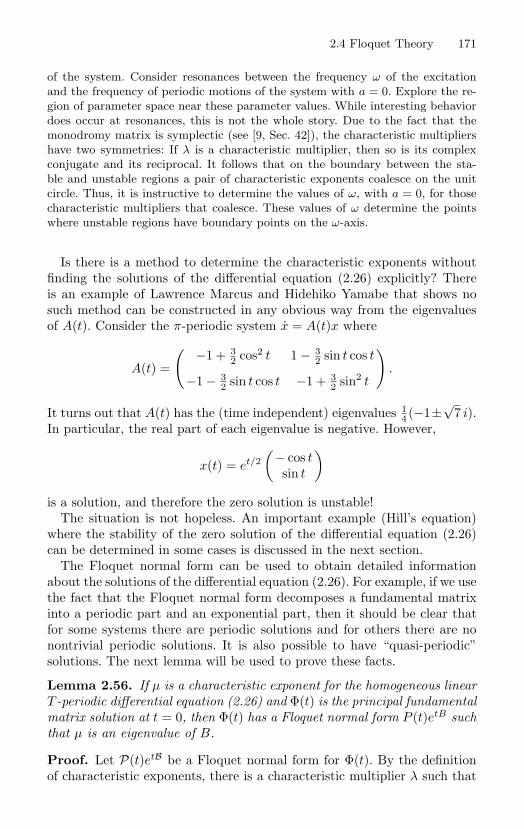
2.4 Floquet Theory 171
of the system. Consider resonances between the frequency ω of the excitationand the frequency of periodic motions of the system with a = 0. Explore the re-gion of parameter space near these parameter values. While interesting behaviordoes occur at resonances, this is not the whole story. Due to the fact that themonodromy matrix is symplectic (see [9, Sec. 42]), the characteristic multipliershave two symmetries: If λ is a characteristic multiplier, then so is its complexconjugate and its reciprocal. It follows that on the boundary between the sta-ble and unstable regions a pair of characteristic exponents coalesce on the unitcircle. Thus, it is instructive to determine the values of ω, with a = 0, for thosecharacteristic multipliers that coalesce. These values of ω determine the pointswhere unstable regions have boundary points on the ω-axis.
Is there is a method to determine the characteristic exponents withoutfinding the solutions of the differential equation (2.26) explicitly? Thereis an example of Lawrence Marcus and Hidehiko Yamabe that shows nosuch method can be constructed in any obvious way from the eigenvaluesof A(t). Consider the π-periodic system x = A(t)x where
A(t) =
(−1 + 3
2 cos2 t 1 − 32 sin t cos t
−1 − 32 sin t cos t −1 + 3
2 sin2 t
).
It turns out that A(t) has the (time independent) eigenvalues 14 (−1±
√7 i).
In particular, the real part of each eigenvalue is negative. However,
x(t) = et/2(
− cos tsin t
)is a solution, and therefore the zero solution is unstable!
The situation is not hopeless. An important example (Hill’s equation)where the stability of the zero solution of the differential equation (2.26)can be determined in some cases is discussed in the next section.
The Floquet normal form can be used to obtain detailed informationabout the solutions of the differential equation (2.26). For example, if we usethe fact that the Floquet normal form decomposes a fundamental matrixinto a periodic part and an exponential part, then it should be clear thatfor some systems there are periodic solutions and for others there are nonontrivial periodic solutions. It is also possible to have “quasi-periodic”solutions. The next lemma will be used to prove these facts.
Lemma 2.56. If µ is a characteristic exponent for the homogeneous linearT -periodic differential equation (2.26) and Φ(t) is the principal fundamentalmatrix solution at t = 0, then Φ(t) has a Floquet normal form P (t)etB suchthat µ is an eigenvalue of B.
Proof. Let P(t)etB be a Floquet normal form for Φ(t). By the definitionof characteristic exponents, there is a characteristic multiplier λ such that
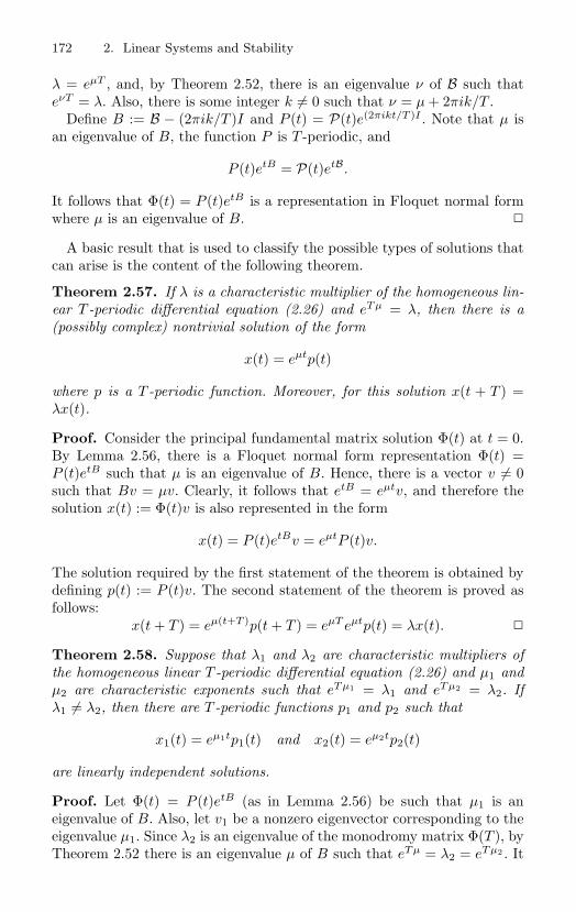
172 2. Linear Systems and Stability
λ = eµT , and, by Theorem 2.52, there is an eigenvalue ν of B such thateνT = λ. Also, there is some integer k = 0 such that ν = µ + 2πik/T .
Define B := B − (2πik/T )I and P (t) = P(t)e(2πikt/T )I . Note that µ isan eigenvalue of B, the function P is T -periodic, and
P (t)etB = P(t)etB.
It follows that Φ(t) = P (t)etB is a representation in Floquet normal formwhere µ is an eigenvalue of B.
A basic result that is used to classify the possible types of solutions thatcan arise is the content of the following theorem.
Theorem 2.57. If λ is a characteristic multiplier of the homogeneous lin-ear T -periodic differential equation (2.26) and eTµ = λ, then there is a(possibly complex) nontrivial solution of the form
x(t) = eµtp(t)
where p is a T -periodic function. Moreover, for this solution x(t + T ) =λx(t).
Proof. Consider the principal fundamental matrix solution Φ(t) at t = 0.By Lemma 2.56, there is a Floquet normal form representation Φ(t) =P (t)etB such that µ is an eigenvalue of B. Hence, there is a vector v = 0such that Bv = µv. Clearly, it follows that etB = eµtv, and therefore thesolution x(t) := Φ(t)v is also represented in the form
x(t) = P (t)etBv = eµtP (t)v.
The solution required by the first statement of the theorem is obtained bydefining p(t) := P (t)v. The second statement of the theorem is proved asfollows:
x(t + T ) = eµ(t+T )p(t + T ) = eµT eµtp(t) = λx(t).
Theorem 2.58. Suppose that λ1 and λ2 are characteristic multipliers ofthe homogeneous linear T -periodic differential equation (2.26) and µ1 andµ2 are characteristic exponents such that eTµ1 = λ1 and eTµ2 = λ2. Ifλ1 = λ2, then there are T -periodic functions p1 and p2 such that
x1(t) = eµ1tp1(t) and x2(t) = eµ2tp2(t)
are linearly independent solutions.
Proof. Let Φ(t) = P (t)etB (as in Lemma 2.56) be such that µ1 is aneigenvalue of B. Also, let v1 be a nonzero eigenvector corresponding to theeigenvalue µ1. Since λ2 is an eigenvalue of the monodromy matrix Φ(T ), byTheorem 2.52 there is an eigenvalue µ of B such that eTµ = λ2 = eTµ2 . It
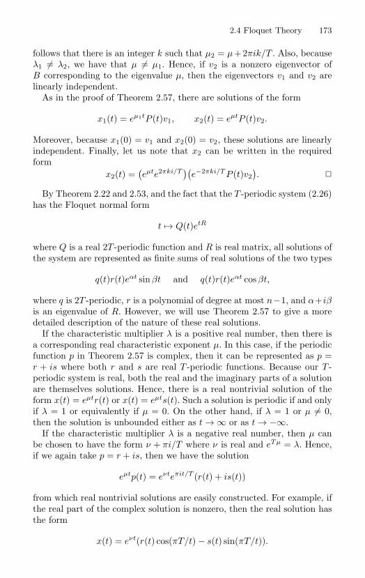
2.4 Floquet Theory 173
follows that there is an integer k such that µ2 = µ+2πik/T . Also, becauseλ1 = λ2, we have that µ = µ1. Hence, if v2 is a nonzero eigenvector ofB corresponding to the eigenvalue µ, then the eigenvectors v1 and v2 arelinearly independent.
As in the proof of Theorem 2.57, there are solutions of the form
x1(t) = eµ1tP (t)v1, x2(t) = eµtP (t)v2.
Moreover, because x1(0) = v1 and x2(0) = v2, these solutions are linearlyindependent. Finally, let us note that x2 can be written in the requiredform
x2(t) =(eµte2πki/T
)(e−2πki/T P (t)v2
).
By Theorem 2.22 and 2.53, and the fact that the T -periodic system (2.26)has the Floquet normal form
t → Q(t)etR
where Q is a real 2T -periodic function and R is real matrix, all solutions ofthe system are represented as finite sums of real solutions of the two types
q(t)r(t)eαt sin βt and q(t)r(t)eαt cos βt,
where q is 2T -periodic, r is a polynomial of degree at most n−1, and α+iβis an eigenvalue of R. However, we will use Theorem 2.57 to give a moredetailed description of the nature of these real solutions.
If the characteristic multiplier λ is a positive real number, then there isa corresponding real characteristic exponent µ. In this case, if the periodicfunction p in Theorem 2.57 is complex, then it can be represented as p =r + is where both r and s are real T -periodic functions. Because our T -periodic system is real, both the real and the imaginary parts of a solutionare themselves solutions. Hence, there is a real nontrivial solution of theform x(t) = eµtr(t) or x(t) = eµts(t). Such a solution is periodic if and onlyif λ = 1 or equivalently if µ = 0. On the other hand, if λ = 1 or µ = 0,then the solution is unbounded either as t → ∞ or as t → −∞.
If the characteristic multiplier λ is a negative real number, then µ canbe chosen to have the form ν + πi/T where ν is real and eTµ = λ. Hence,if we again take p = r + is, then we have the solution
eµtp(t) = eνteπit/T (r(t) + is(t))
from which real nontrivial solutions are easily constructed. For example, ifthe real part of the complex solution is nonzero, then the real solution hasthe form
x(t) = eνt(r(t) cos(πT/t) − s(t) sin(πT/t)).
174 2. Linear Systems and Stability
Such a solution is periodic if and only if λ = −1 or equivalently if ν = 0.In this case the solution is 2T -periodic. If ν = 0, then the solution isunbounded.
If λ is complex, then we have µ = α+ iβ and there is a solution given by
x(t) = eαt(cos βt + i sin βt)(r(t) + is(t)).
Thus, there are real solutions
x1(t) = eαt(r(t) cos βt − s(t) sin βt),x2(t) = eαt(r(t) sin βt + s(t) cos βt).
If α = 0, then both solutions are unbounded. If α = 0 and if there arerelatively prime positive integers m and n such that 2πm/β = nT , thenthe solution is nT -periodic. If no such integers exist, then the solution iscalled quasi-periodic.
We will prove in Section 2.4.4 that the stability of a periodic orbit is de-termined by the stability of the corresponding fixed point of a Poincare mapdefined on a Poincare section that meets the periodic orbit. Generically, thestability of the fixed point of the Poincare map is determined by the eigen-values of its derivative at the fixed point. For example, if the eigenvaluesof the derivative of the Poincare map at the fixed point corresponding tothe periodic orbit are all inside the unit circle, then the periodic orbit isasymptotically stable. It turns out that the eigenvalues of the derivative ofthe Poincare map are closely related to the characteristic multipliers of atime-periodic system, namely, the variational equation along the periodicorbit. We will have much more to say about the general case later. Herewe will illustrate the idea for an example where the Poincare map is easyto compute.
Suppose that
u = f(u, t), u ∈ Rn (2.27)
is a smooth nonautonomous differential equation. If there is some T > 0such that f(u, t + T ) = f(u, t) for all u ∈ R
n and all t ∈ R, then thesystem (2.27) is called T -periodic.
The nonautonomous system (2.27) is made “artificially” autonomous bythe addition of a new equation as follows:
u = f(u, ψ), ψ = 1 (2.28)
where ψ may be viewed as an angular variable modulo T . In other words,we can consider ψ + nT = ψ whenever n is an integer. The phase cylinderfor system (2.28) is R
n×T, where T (topologically the unit circle) is definedto be R modulo T . This autonomous system provides the correct geometrywith which to define a Poincare map.
2.4 Floquet Theory 175
For each ξ ∈ Rn, let t → u(t, ξ) denote the solution of the differential
equation (2.27) such that u(0, ξ) = ξ, and note that t → (u(t, ξ), t) is thecorresponding solution of the system (2.28). The set Σ := (ξ, ψ) : ψ = 0is a Poincare section, and the corresponding Poincare map is given byξ → u(T, ξ).
If there is a point p ∈ Rn such that f(p, t) = 0 for all t ∈ R, then the
function t → (p, t), or equivalently t → (u(t, p), t), is a periodic solution ofthe system (2.28) with period T . Moreover, let us note that u(T, p) = p.Thus, the periodic solution corresponds to a fixed point of the Poincaremap as it should.
The derivative of the Poincare map at p is the linear transformation ofR
n given by the partial derivative uξ(T, p). Moreover, by differentiatingboth the differential equation (2.27) and the initial condition u(0, ξ) = ξwith respect to ξ, it is easy to see that the matrix function t → uξ(t, p)is the principal fundamental matrix solution at t = 0 of the (T -periodiclinear) variational initial value problem
W = fu(u(t, p), t)W, W (0) = I. (2.29)
If the solution of system (2.29) is represented in the Floquet normal formuξ(t, p) = P (t)etB , then the derivative of the Poincare map is given byuξ(T, p) = eTB . In particular, the characteristic multipliers of the vari-ational equation (2.29) coincide with the eigenvalues of the derivative ofthe Poincare map. Thus, whenever the principle of linearized stability isvalid, the stability of the periodic orbit is determined by the characteristicmultipliers of the periodic variational equation (2.29).
As an example, consider the pendulum with oscillating support
θ + (1 + a cos ωt) sin θ = 0.
The zero solution, given by θ(t) ≡ 0, corresponds to a 2π/ω-periodic so-lution of the associated autonomous system. A calculation shows that thevariational equation along this periodic solution is equivalent to the secondorder differential equation
x + (1 + a cos ωt)x = 0,
called a Mathieu equation.Since, as we have just seen (see also Exercise 2.55), equations of Mathieu
type arise frequently in applications, the Floquet analysis of such equationsis important. In Section 2.4.2 we will show how the stability of the zero solu-tion of the Mathieu equation, and, in turn, the stability of the zero solutionof the pendulum with oscillating support, is related in a delicate mannerto the amplitude a and the frequency ω of the periodic displacement.
176 2. Linear Systems and Stability
Exercise 2.59. This is a continuation of Exercise 2.30. Suppose that v : R →R
3 is a periodic function. Consider the differential equation
x = v(t) × x
and discuss the stability of its periodic solutions.
2.4.1 Lyapunov ExponentsAn important generalization of Floquet exponents, called Lyapunov expo-nents, are introduced in this section. This concept is used extensively inthe theory of dynamical systems (see, for example, [80], [114], [134], and[185]).
Consider a (nonlinear) differential equation
u = f(u), u ∈ Rn (2.30)
with flow ϕt. If ε ∈ R, ξ, v ∈ Rn, and η := ξ + εv, then the two solutions
t → ϕt(ξ), t → ϕt(ξ + εv)
start at points that are O(ε) close; that is, the absolute value of the differ-ence of the two points in R
n is bounded by the usual norm of v times ε.Moreover, by Taylor expansion at ε = 0, we have that
ϕt(ξ + εv) − ϕt(ξ) = εDϕt(ξ)v + O(ε2)
where Dϕt(ξ) denotes the derivative of the function u → ϕt(u) evaluated atu = ξ. Thus, the first order approximation of the difference of the solutionsat time t is εDϕt(ξ)v where t → Dϕt(ξ) is the principal fundamental matrixsolution at t = 0 of the linearized equation
W = Df(ϕt(ξ))W
along the solution of the original system (2.30) starting at ξ. To see thisfact, just note that
ϕt(u) = f(ϕt(u))
and differentiate both sides of this identity with respect to u at u = ξ.If we view v as a vector in the tangent space to R
n at ξ, denoted TξRn,
then Dϕt(ξ)v is a vector in the tangent space Tϕt(ξ)Rn. For each such v,
if v = 0, then it is natural to define a corresponding linear operator L,from the linear subspace of TξR
n generated by v to the linear subspaceof Tϕt(ξ)R
n generated by Dϕt(ξ)v, defined by L(av) = Dϕt(ξ)av wherea ∈ R. Let us note that the norm of this operator measures the relative“expansion” or “contraction” of the vector v; that is,
‖L‖ = supa=0
‖Dφt(ξ)av‖‖av‖ =
‖Dφt(ξ)v‖‖v‖ .
2.4 Floquet Theory 177
Our two solutions can be expressed in integral form; that is,
ϕt(ξ) = ξ +∫ t
0f(ϕs(ξ)) ds,
ϕt(ξ + εv) = ξ + εv +∫ t
0f(ϕs(ξ + εv)) ds.
Hence, as long as we consider a finite time interval or a solution that iscontained in a compact subset of R
n, there is a Lipschitz constant Lip(f) >0 for the function f , and we have the inequality
‖ϕt(ξ + εv) − ϕt(ξ)‖ ≤ ε‖v‖ + Lip(f)∫ t
0‖ϕs(ξ + εv) − ϕs(ξ)‖ ds.
By Gronwall’s inequality, the separation distance between the solutions isbounded by an exponential function of time. In fact, we have the estimate
‖ϕt(ξ + εv) − ϕt(ξ)‖ ≤ ε‖v‖et Lip(f).
The above computation for the norm of L and the fact that the separationrate between two solutions is at most exponential motivates the followingdefinition (see [114]).
Definition 2.60. If, for some ξ ∈ Rn, the solution t → ϕt(ξ) of the differ-
ential equation (2.30) is defined for all t ≥ 0, and if v ∈ Rn is a nonzero
vector, then the Lyapunov exponent at ξ in the direction v for the flow ϕt
is
χ(p, v) := lim supt→∞
1t
ln(‖Dφt(ξ)v‖
‖v‖
).
As a simple example, let us consider the planar system
x = −ax, y = by
where a and b are positive parameters, and let us note that its flow is givenby
ϕt(x, y) = (e−atx, ebty).
By an easy computation using the definition of the Lyapunov exponents,it follows that if v is given by v = (w, z) and z = 0, then χ(ξ, v) = b. Ifz = 0 and w = 0, then χ(ξ, v) = −a. In particular, there are exactly twoLyapunov exponents for this system. Of course, the Lyapunov exponentsin this case correspond to the eigenvalues of the system matrix.
Although our definition of Lyapunov exponents is for autonomous sys-tems, it should be clear that since the definition only depends on the funda-mental matrix solutions of the associated variational equations along orbits
178 2. Linear Systems and Stability
of the system, we can define the same notion for solutions of abstract time-dependent linear systems. Indeed, for a T -periodic linear system
u = A(t)u, u ∈ Rn (2.31)
with principal fundamental matrix Φ(t) at t = 0, the Lyapunov exponentdefined with respect to the nonzero vector v ∈ R
n is
χ(v) := lim supt→∞
1t
ln(‖Φ(t)v‖
‖v‖
).
Proposition 2.61. If µ is a Floquet exponent of the system (2.31), thenthe real part of µ is a Lyapunov exponent.
Proof. Let us suppose that the principal fundamental matrix Φ(t) is givenin Floquet normal form by
Φ(t) = P (t)etB .
If µ = a + bi is a Floquet exponent, then there is a corresponding vectorv such that eTBv = eµT v. Hence, using the Floquet normal form, we havethat
Φ(T )v = eµT v.
If t ≥ 0, then there is a nonnegative integer n and a number r such that0 ≤ r < T and
1t
ln(‖Φ(t)v‖
‖v‖
)=
1T
( nT
nT + r
)( 1n
ln(‖P (nT + r)erBenµT v‖
‖v‖
))=
1T
( nT
nT + r
)( 1n
ln |enTa| +1n
ln(‖P (r)erBv‖
‖v‖
)).
Clearly, n → ∞ as t → ∞. Thus, it is easy to see that
limt→∞
1T
( nT
nT + r
)( 1n
ln |enTa| +1n
ln(‖P (r)erBv‖
‖v‖
))= a.
Let us suppose that a differential equation has a compact invariant setthat contains an orbit whose closure is dense in the invariant set. Then,the existence of a positive Lyapunov exponent for this orbit ensures thatnearby orbits tend to separate exponentially fast from the dense orbit.However, since these orbits are confined to a compact invariant set, theymust also be bounded. This suggests that each small neighborhood in theinvariant set undergoes both stretching and folding as it evolves with theflow. The subsequent kneading of the invariant set due to this stretchingand folding would tend to mix the evolving neighborhoods so that they

2.4 Floquet Theory 179
eventually intertwine in a complicated manner. For this reason, the ex-istence of a positive Lyapunov exponent is often taken as a signature of“chaos.” While this criterion is not always valid, the underlying idea thatthe stretching implied by a positive Lyapunov exponent is associated withcomplex motions is important in the modern theory of dynamical systems.
Exercise 2.62. Show that if two points are on the same orbit, then the corre-sponding Lyapunov exponents are the same.
Exercise 2.63. Prove the “converse” of Proposition 2.61; that is, every Lya-punov exponent for a time-periodic system is a Floquet exponent.
Exercise 2.64. If x = f(x), determine the Lyapunov exponent χ(ξ, f(ξ)).
Exercise 2.65. How many Lyapunov exponents are associated with an orbitof a differential equation in an n-dimensional phase space.
Exercise 2.66. Suppose that x is in the omega limit set of an orbit. Are theLyapunov exponents associated with x the same as those associated with theoriginal orbit?
Exercise 2.67. In all the examples in this section, the lim sup can be replacedby lim. Are there examples where the superior limit is a finite number, but thelimit does not exist? This is (probably) a challenging exercise! For an answersee [114] and [134].
2.4.2 Hill’s EquationA famous example where Floquet theory applies to give good stabilityresults is Hill’s equation,
u + a(t)u = 0, a(t + T ) = a(t).
This equation was introduced by George W. Hill in his study of the motionsof the moon. Roughly speaking, the motion of the moon can be viewed asa harmonic oscillator in a periodic gravitational field. However, this modelequation arises in many areas of applied mathematics where the stability ofperiodic motions is an issue. A prime example, mentioned in the previoussection, is the stability analysis of small oscillations of a pendulum whoselength varies with time.
If we define
x :=(
uu
),
then Hill’s equation is equivalent to the first order system x = A(t)x where
A(t) =(
0 1−a(t) 0
).
180 2. Linear Systems and Stability
We will apply linear systems theory, especially Floquet theory, to analyzethe stability of the zero solution of this linear T -periodic system.
The first step in the stability analysis is an application of Liouville’sformula (2.15). In this regard, you may recall from your study of scalarsecond order linear differential equations that if u + p(t)u + q(t)u = 0 andthe Wronskian of the two solutions u1 and u2 is defined by
W (t) := det(
u1(t) u2(t)u1(t) u2(t)
),
then
W (t) = W (0)e− ∫ t0 p(s) ds. (2.32)
Note that for the equivalent first order system
x =(
0 1−q(t) −p(t)
)x = B(t)x
with fundamental matrix Ψ(t), formula (2.32) is a special case of Liouville’sformula
det Ψ(t) = det Ψ(0)e∫ t0 tr B(s)ds.
At any rate, let us apply Liouville’s formula to the principal fundamentalmatrix Φ(t) at t = 0 for Hill’s system to obtain the identity det Φ(t) ≡ 1.Since the determinant of a matrix is the product of the eigenvalues ofthe matrix, we have an important fact: The product of the characteristicmultipliers of the monodromy matrix, Φ(T ), is 1.
Let the characteristic multipliers for Hill’s equation be denoted by λ1and λ2 and note that they are roots of the characteristic equation
λ2 − (tr Φ(T ))λ + det Φ(T ) = 0.
For notational convenience let us set 2φ = tr Φ(T ) to obtain the equivalentcharacteristic equation
λ2 − 2φλ + 1 = 0
whose solutions are given by
λ = φ ±√
φ2 − 1.
There are several cases to consider depending on the value of φ.Case 1: If φ > 1, then λ1 and λ2 are distinct positive real numbers such
that λ1λ2 = 1. Thus, we may assume that 0 < λ1 < 1 < λ2 with λ1 = 1/λ2and there is a real number µ > 0 (a characteristic exponent) such thateTµ = λ2 and e−Tµ = λ1. By Theorem 2.57 and Theorem 2.58, there is afundamental set of solutions of the form
e−µtp1(t), eµtp2(t)
2.4 Floquet Theory 181
where the real functions p1 and p2 are T -periodic. In this case, the zerosolution is unstable.
Case 2: If φ < −1, then λ1 and λ2 are both real and both negative. Also,since λ1λ2 = 1, we may assume that λ1 < −1 < λ2 < 0 with λ1 = 1/λ2.Thus, there is a real number µ > 0 (a characteristic exponent) such thate2Tµ = λ2
1 and e−2Tµ = λ22. As in Case 1, there is a fundamental set of
solutions of the form
eµtq1(t), e−µtq2(t)
where the real functions q1 and q2 are 2T -periodic. Again, the zero solutionis unstable.
Case 3: If −1 < φ < −1, then λ1 and λ2 are complex conjugates eachwith nonzero imaginary part. Since λ1λ1 = 1, we have that |λ1| = 1, andtherefore both characteristic multipliers lie on the unit circle in the complexplane. Because both λ1 and λ2 have nonzero imaginary parts, one of thesecharacteristic multipliers, say λ1, lies in the upper half plane. Thus, there isa real number θ with 0 < θT < π and eiθT = λ1. In fact, there is a solutionof the form eiθt(r(t)+ is(t)) with r and s both T -periodic functions. Hence,there is a fundamental set of solutions of the form
r(t) cos θt − s(t) sin θt, r(t) sin θt + s(t) cos θt.
In particular, the zero solution is stable (see Exercise 2.69) but not asymp-totically stable. Also, the solutions are periodic if and only if there arerelatively prime positive integers m and n such that 2πm/θ = nT . If suchintegers exist, all solutions have period nT . If not, then these solutions arequasi-periodic.
We have just proved the following facts for Hill’s equation: Suppose thatΦ(t) is the principal fundamental matrix solution of Hill’s equation at t = 0.If | tr Φ(T )| < 2, then the zero solution is stable. If | tr Φ(T )| > 2, then thezero solution is unstable.
Case 4: If φ = 1, then λ1 = λ2 = 1. The nature of the solutions dependson the canonical form of Φ(T ). If Φ(T ) is the identity, then e0 = Φ(T ) andthere is a Floquet normal form Φ(t) = P (t) where P (t) is T -periodic andinvertible. Thus, there is a fundamental set of periodic solutions and thezero solution is stable. If Φ(T ) is not the identity, then there is a nonsingularmatrix C such that
CΦ(T )C−1 = I + N = eN
where N = 0 is nilpotent. Thus, Φ(t) has a Floquet normal form Φ(t) =P (t)etB where B := C−1( 1
T N)C. Because
etB = C−1(I +t
TN)C,
182 2. Linear Systems and Stability
the matrix function t → etB is unbounded, and therefore the zero solutionis unstable.
Case 5: If φ = −1, then the situation is similar to Case 4, except thefundamental matrix is represented by Q(t)etB where Q(t) is a 2T -periodicmatrix function.
By the results just presented, the stability of Hill’s equation is reduced,in most cases, to a determination of the absolute value of the trace ofits principal fundamental matrix evaluated after one period. While this isa useful fact, it leaves open an important question: Can the stability bedetermined without imposing a condition on the solutions of the equation?It turns out that in some special cases this is possible (see [115] and [189]).A theorem of Lyapunov [114] in this direction follows.
Theorem 2.68. If a : R → R is a positive T -periodic function such that
T
∫ T
0a(t) dt ≤ 4,
then all solutions of the Hill’s equation x + a(t)x = 0 are bounded. Inparticular, the trivial solution is stable.
The proof of Theorem 2.68 is outlined in Exercises 2.69 and 2.74.
Exercise 2.69. Prove: If all solutions of the T -periodic system x = A(t)x arebounded, then the trivial solution is Lyapunov stable.
Exercise 2.70. Consider the second order system
u + u + cos(t) u = 0.
Prove: If ρ1 and ρ2 are the characteristic multipliers of the corresponding firstorder system, then ρ1ρ2 = exp(−2π). Also, show that this result implies thePoincare map for the system is dissipative; that is, it contracts area.
Exercise 2.71. Prove: The equation
u − (2 sin2 t)u + (1 + sin 2t)u = 0.
does not have a fundamental set of periodic solutions.
Exercise 2.72. Discuss the stability of the trivial solution of the scalar time-periodic system x = (cos2 t)x.
Exercise 2.73. Prove: The zero solution is unstable for the system x = A(t)xwhere
A(t) :=(
1/2 − cos t 12147 3/2 + sin t
).
Exercise 2.74. Prove Theorem 2.68. Hint: If Hill’s equation has an unboundedsolution, then there is a real solution t → x(t) and a real Floquet multiplier suchthat x(t + T ) = λx(t). Define a new function t → u(t) by
u(t) :=x(t)x(t)
,
2.4 Floquet Theory 183
and show that u is a solution of the Riccati equation
u = −a(t) − u2.
Use the Riccati equation to prove that the solution x has at least one zero in theinterval [0, T ]. Also, show that x has two distinct zeros on some interval whoselength does not exceed T . Finally, use the following proposition to finish theproof. If f is a smooth function on the finite interval [α, β] such that f(α) = 0,f(β) = 0, and such that f is positive on the open interval (α, β), then
(β − α)∫ β
α
|f ′′(t)|f(t)
dt > 4.
To prove this proposition, first suppose that f attains its maximum at γ andshow that
4β − α
≤ 1γ − α
+1
β − γ=
1f(γ)
(f(γ) − f(α)γ − α
− f(β) − f(γ)β − γ
).
Then, use the mean value theorem and the fundamental theorem of calculus tocomplete the proof.
Exercise 2.75. Prove: If t → a(t) is negative, then the Hill’s equation x +a(t)x = 0 has an unbounded solution. Hint: Multiply by x and integrate byparts.
2.4.3 Periodic Orbits of Linear SystemsIn this section we will consider the existence and stability of periodic solu-tions of the time-periodic system
x = A(t)x + b(t), x ∈ Rn (2.33)
where t → A(t) is a T -periodic matrix function and t → b(t) is a T -periodicvector function.
Theorem 2.76. If the number one is not a characteristic multiplier of theT -periodic homogeneous system x = A(t)x, then (2.33) has at least oneT -periodic solution.
Proof. Let us show first that if t → x(t) is a solution of system (2.33)and x(0) = x(T ), then this solution is T -periodic. Define y(t) := x(t + T ).Note that t → y(t) is a solution of (2.33) and y(0) = x(0). Thus, by theuniqueness theorem x(t + T ) = x(t) for all t ∈ R.
If Φ(t) is the principal fundamental matrix solution of the homogeneoussystem at t = 0, then, by the variation of constants formula,
x(T ) = Φ(T )x(0) + Φ(T )∫ T
0Φ−1(s)b(s) ds.
184 2. Linear Systems and Stability
Therefore, x(T ) = x(0) if and only if
(I − Φ(T ))x(0) = Φ(T )∫ T
0Φ−1(s)b(s) ds.
This equation for x(0) has a solution whenever the number one is not aneigenvalue of Φ(T ). (Note that the map x(0) → x(T ) is the Poincare map.Thus, our periodic solution corresponds to a fixed point of the Poincaremap).
By Floquet’s theorem, there is a matrix B such that the monodromymatrix is given by
Φ(T ) = eTB .
In other words, by the hypothesis, the number one is not an eigenvalue ofΦ(T ).
Corollary 2.77. If A(t) = A, a constant matrix such that A is infinitesi-mally hyperbolic (no eigenvalues on the imaginary axis), then the differen-tial equation (2.33) has at least one T -periodic solution.
Proof. The monodromy matrix eTA does not have 1 as an eigenvalue.
Exercise 2.78. Discuss the uniqueness of the T -periodic solutions of the sys-tem (2.33). Also, using Theorem 2.53, discuss the stability of the T -periodicsolutions.
In system (2.33) if b = 0, then the trivial solution is a T -periodic solution.The next theorem states a general sufficient condition for the existence ofa T -periodic solution.
Theorem 2.79. If the T -periodic system (2.33) has a bounded solution,then it has a T -periodic solution.
Proof. Consider the principal fundamental matrix solution Φ(t) at t = 0 ofthe homogeneous system corresponding to the differential equation (2.33).By the variation of constants formula, we have the equation
x(T ) = Φ(T )x(0) + Φ(T )∫ T
0Φ−1(s)b(s) ds.
Also, by Theorem 2.47, there is a constant matrix B such that Φ(T ) = eTB .Thus, the stroboscopic Poincare map P is given by
P (ξ) := Φ(T )ξ + Φ(T )∫ T
0Φ−1(s)b(s) ds
= eTB(ξ +
∫ T
0Φ−1(s)b(s) ds
).
2.4 Floquet Theory 185
If the solution with initial condition x(0) = ξ0 is bounded, then thesequence P j(ξ0)∞
j=0 is bounded. Also, P is an affine map; that is, P (ξ) =Lξ + y where L = eTB = Φ(T ) is a real invertible linear map and y is anelement of R
n.Note that if there is a point x ∈ R
n such that P (x) = x, then thesystem (2.33) has a periodic orbit. Thus, if we assume that there are noperiodic orbits, then the equation
(I − L)ξ = y
has no solution ξ. In other words, y is not in the range R of the operatorI − L.
There is some vector v ∈ Rn such that v is orthogonal to R and the
inner product 〈v, y〉 does not vanish. Moreover, because v is orthogonal tothe range, we have
〈(I − L)ξ, v〉 = 0
for each ξ ∈ Rn, and therefore
〈ξ, v〉 = 〈Lξ, v〉. (2.34)
Using the representation P (ξ) = Lξ + y and an induction argument, itis easy to prove that if j is a nonnegative integer, then P j(ξ0) = Ljξ0 +∑j−1
k=0 Lky. By taking the inner product with v and repeatedly applyingthe reduction formula (2.34), we have
〈P j(ξ0), v〉 = 〈ξ0, v〉 + (j − 1)〈y, v〉.
Moreover, because 〈v, y〉 = 0, it follows immediately that
limj→∞
〈P j(ξ0), v〉 = ∞,
and therefore the sequence P j(ξ0)∞j=0 is unbounded, in contradiction.
2.4.4 Stability of Periodic OrbitsConsider a (nonlinear) autonomous system of differential equations on R
n
given by u = f(u) with a periodic orbit Γ. Also, for each ξ ∈ Rn, define
the vector function t → u(t, ξ) to be the solution of this system with theinitial condition u(0, ξ) = ξ.
If p ∈ Γ and Σ′ ⊂ Rn is a section transverse to f(p) at p, then, as a
corollary of the implicit function theorem, there is an open set Σ ⊆ Σ′ anda function T : Σ → R, the time of first return to Σ′, such that for eachσ ∈ Σ, we have u(T (σ), σ) ∈ Σ′. The map P, given by σ → u(T (σ), σ), isthe Poincare map corresponding to the Poincare section Σ.
186 2. Linear Systems and Stability
The Poincare map is defined only on Σ, a manifold contained in Rn. It
is convenient to avoid choosing local coordinates on Σ. Thus, we will viewthe elements in Σ also as points in the ambient space R
n. In particular, ifv ∈ R
n is tangent to Σ at p, then the derivative of P in the direction v isgiven by
DP(p)v = (dT (p)v)f(p) + uξ(T (p), p)v. (2.35)
The next proposition relates the spectrum of DP(p) to the Floquet multi-pliers of the first variational equation
W = Df(u(t, p))W.
Proposition 2.80. If Γ is a periodic orbit and p ∈ Γ, then the union ofthe set of eigenvalues of the derivative of a Poincare map at p ∈ Γ and thesingleton set 1 is the same as the set of characteristic multipliers of thefirst variational equation along Γ. In particular, zero is not an eigenvalue.
Proof. Recall that t → uξ(t, ξ) is the principal fundamental matrix solu-tion at t = 0 of the first variational equation and, since
d
dtf(u(t, ξ)) = Df(u(t, ξ)ut(t, ξ) = Df(u(t, ξ)f(u(t, ξ)),
the vector function t → f(u(t, ξ)) is the solution of the variational equationwith the initial condition W (0) = f(ξ). In particular,
uξ(T (p), p)f(p) = f(u(T (p), p)) = f(p),
and therefore f(p) is an eigenvector of the linear transformation uξ(T (p), p)with eigenvalue the number one.
Since Σ is transverse to f(p), there is a basis of Rn of the form
f(p), s1, . . . , sn−1
with si tangent to Σ at p for each i = 1, . . . , n − 1. It follows that thematrix uξ(T (p), p) has block form, relative to this basis, given by(
1 a0 b
)where a is 1 × (n − 1) and b is (n − 1) × (n − 1). Moreover, each v ∈ R
n
that is tangent to Σ at p has block form (the transpose of) (0, vΣ). As aresult, we have the equality
uξ(T (p), p)v =(
1 a0 b
)(0vΣ
).
2.4 Floquet Theory 187
Using (2.35), the block form of uξ(T (p), p), and the fact that the rangeof DP(p) is tangent to Σ at p, it follows that
DP(p)v =(
dT (p)v + avΣbvΣ
)=
(0
bvΣ
).
In other words, the derivative of the Poincare map may be identified withb and the differential of the return time map with −a. In particular, theeigenvalues of the derivative of the Poincare map coincide with the eigen-values of b.
Exercise 2.81. Prove that the characteristic multipliers of the first variationalequation along a periodic orbit do not depend on the choice of p ∈ Γ.
Most of the rest of this section is devoted to a proof of the followingfundamental theorem.
Theorem 2.82. Suppose that Γ is a periodic orbit for the autonomousdifferential equation u = f(u) and P is a corresponding Poincare mapdefined on a Poincare section Σ such that p ∈ Γ ∩ Σ. If the eigenvalues ofthe derivative DP(p) are inside the unit circle in the complex plane, thenΓ is asymptotically stable.
There are several possible proofs of this theorem. The approach usedhere is adapted from [95].
To give a complete proof of Theorem 2.82, we will require several prelim-inary results. Our first objective is to show that the point p is an asymptot-ically stable fixed point of the dynamical system defined by the Poincaremap on Σ.
Let us begin with a useful simple replacement of the Jordan normal formtheorem that is adequate for our purposes here (see [99]).
Proposition 2.83. An n×n (possibly complex) matrix A is similar to anupper triangular matrix whose diagonal elements are the eigenvalues of A.
Proof. Let v be a nonzero eigenvector of A corresponding to the eigenvalueλ. The vector v can be completed to a basis of C
n that defines a matrixQ partitioned by the corresponding column vectors Q := [v, y1, . . . , yn−1].Moreover, Q is invertible and
[Q−1v, Q−1y1, . . . , Q−1yn−1] = [e1, . . . , en]
where e1, . . . , en denote the usual basis elements.Note that
Q−1AQ = Q−1[λv, Ay1, . . . , Ayn−1]= [λe1, Q
−1Ay1, . . . , Q−1Ayn−1].
188 2. Linear Systems and Stability
In other words, the matrix Q−1AQ is given in block form by
Q−1AQ =(
λ ∗0 A
)where A is an (n−1)×(n−1) matrix. In particular, this proves the theoremfor all 2 × 2 matrices.
By induction, there is an (n − 1) × (n − 1) matrix R such that R−1ARis upper triangular. The matrix (QR)−1AQR where
R =(
1 00 R
)is an upper triangular matrix with the eigenvalues of A as its diagonalelements, as required.
Let ρ(A) denote the spectral radius of A, that is, the maximum modulusof the eigenvalues of A.
Proposition 2.84. Suppose that A is an n×n matrix. If ε > 0, then thereis a norm on C
n such that ‖A‖ε < ρ(A) + ε. If A is a real matrix, then therestriction of the “ε-norm” to R
n is a norm on Rn with the same property.
Proof. The following proof is adapted from [99]. By Proposition 2.83, thereis a matrix Q such that
QAQ−1 = D + N
where D is diagonal with the eigenvalues of A as its diagonal elements, andN is upper triangular with each of its diagonal elements equal to zero.
Let µ > 0, and define a new diagonal matrix S with diagonal elements
1, µ−1, µ−2, . . . , µ1−n.
A computation shows that
S(D + N)S−1 = D + SNS−1.
Also, it is easy to show—by writing out the formulas for the components—that every element of the matrix SNS−1 is O(µ).
Define a norm on Cn, by the formula
‖v‖µ := ‖SQv‖ = 〈SQv, SQv〉
where the angle brackets on the right hand side denote the usual Euclideaninner product on C
n. It is easy to verify that this procedure indeed definesa norm on C
n that depends on the parameter µ.Post multiplication by SQ of both sides of the equation
SQAQ−1S−1 = D + SNS−1
2.4 Floquet Theory 189
yields the formula
SQA = (D + SNS−1)SQ.
Using this last identity we have that
‖Av‖2µ = ‖SPAv‖2 = ‖(D + SNS−1)SQv‖2.
Let us define w := SQv and then expand the last norm into inner productsto obtain
‖Av‖2µ = 〈Dw, Dw〉 + 〈SNS−1w, Dw〉
+〈Dw, SNS−1w〉 + 〈SNS−1w, SNS−1w〉.
A direct estimate of the first inner product together with an applicationof the Schwarz inequality to each of the other inner products yields thefollowing estimate:
‖Av‖2µ ≤ (ρ2(A) + O(µ))‖w‖2.
Moreover, we have that ‖v‖µ = ‖w‖. In particular, if ‖v‖µ = 1 then ‖w‖ =1, and it follows that
‖A‖2µ ≤ ρ2(A) + O(µ).
Thus, if µ > 0 is sufficiently small, then ‖A‖µ < ρ(A) + ε, as required.
Corollary 2.85. If all the eigenvalues of the n × n matrix A are insidethe unit circle in the complex plane, then there is an “adapted norm” anda number λ, with 0 < λ < 1, such that ‖Av‖a < λ‖v‖a for all vectors v,real or complex. In particular A is a contraction with respect to the adaptednorm. Moreover, for each norm on R
n or Cn, there is a positive number C
such that ‖Anv‖ ≤ Cλn‖v‖ for all nonnegative integers n.
Proof. Under the hypothesis, we have ρ(A) < 1; thus, there is a numberλ such that ρ(A) < λ < 1. Using Proposition 2.84, there is an adaptednorm so that ‖A‖a < λ. This proves the first part of the corollary. Toprove the second part, recall that all norms on a finite dimensional spaceare equivalent. In particular, there are positive numbers C1 and C2 suchthat
C1‖v‖ ≤ ‖v‖a ≤ C2‖v‖
for all vectors v. Thus, we have
C1‖Anv‖ ≤ ‖Anv‖a ≤ ‖A‖na‖v‖a ≤ C2λ
n‖v‖.
After dividing both sides of the last inequality by C1 > 0, we obtain thedesired estimate.
190 2. Linear Systems and Stability
We are now ready to return to the dynamics of the Poincare map Pdefined above. Recall that Γ is a periodic orbit for the differential equationu = f(u) and P : Σ → Σ′ is defined by P(σ) = u(T (σ), σ) where T is thereturn time function. Also, we have that p ∈ Γ ∩ Σ.
Lemma 2.86. Suppose that V ⊆ Rn is an open set with compact closure
V such that Γ ⊂ V and V is contained in the domain of the function f . Ift∗ ≥ 0, then there is an open set W ⊆ V that contains Γ and is such that,for each point ξ ∈ W , the solution t → u(t, ξ) is defined and stays in V onthe interval 0 ≤ t ≤ t∗. Moreover, if ξ and ν are both in W and 0 ≤ t ≤ t∗,then there is a number L > 0 such that
‖u(t, ξ) − u(t, ν)‖ < ‖ξ − ν‖eLt∗ .
Proof. Using the fact that V is a compact subset of the domain of f andLemma 2.40, the function f is globally Lipschitz on V with a Lipschitzconstant L > 0. Also, there is a minimum positive distance m from theboundary of V to Γ.
An easy application of Gronwall’s inequality can be used to show that ifξ, ν ∈ V , then
‖u(t, ξ) − u(t, ν)‖ ≤ ‖ξ − ν‖eLt (2.36)
for all t such that both solutions are defined on the interval [0, t].Define the set
Wq := ξ ∈ Rn : ‖ξ − q‖eLt∗ < m
and note that Wq is open. If ξ ∈ Wq, then
‖ξ − q‖ < me−Lt∗ < m.
Thus, it follows that Wq ⊆ V .Using the extensibility theorem (Theorem 1.186), it follows that if ξ ∈
Wq, then the interval of existence of the solution t → u(t, ξ) can be extendedas long as the orbit stays in the compact set V . The point q is on the periodicorbit Γ. Thus, the solution t → u(t, q) is defined for all t ≥ 0. Using thedefinition of Wq and an application of the inequality (2.36) to the solutionsstarting at ξ and q, it follows that the solution t → u(t, ξ) is defined andstays in V on the interval 0 ≤ t ≤ t∗.
The union W :=⋃
q∈Γ Wq is an open set in V containing Γ with theproperty that all solutions starting in W remain in V at least on the timeinterval 0 ≤ t ≤ t∗.
Define the distance of a point q ∈ Rn to a set S ⊆ R
n by
dist(q, S) = infx∈S
|q − x|
2.4 Floquet Theory 191
where the norm on the right hand side is the usual Euclidean norm. Simi-larly, the (minimum) distance between two sets is defined as
dist(A, B) = inf|a − b| : a ∈ A, b ∈ B.
(Warning: dist is not a metric.)
Proposition 2.87. If σ ∈ Σ and if limn→∞ Pn(σ) = p, then
limt→∞ dist(u(t, σ), Γ) = 0.
Proof. Let ε > 0 be given and let Σ0 be an open subset of Σ such thatp ∈ Σ0 and such that Σ0, the closure of Σ0, is a compact subset of Σ. Thereturn time map T is continuous; hence, it is uniformly bounded on the setΣ0, that is,
supT (η) : η ∈ Σ0 = T ∗ < ∞.
Let V be an open subset of Rn with compact closure V such that Γ ⊂ V
and V is contained in the domain of f . By Lemma 2.86, there is an openset W ⊆ V such that Γ ⊂ W and such that, for each ξ ∈ W , the solutionstarting at ξ remains in V on the interval 0 ≤ s ≤ T ∗.
Choose δ > 0 so small that the set
Σδ := η ∈ Σ : |η − p| < δ
is contained in W ∩ Σ0, and such that
|η − p|eLT ∗< minm, ε
for all η ∈ Σδ. By Lemma 2.86, if η ∈ Σδ, then, for 0 ≤ s ≤ T ∗, we havethat
|u(s, η) − u(s, p)| < ε.
By the hypothesis, there is some integer N > 0 such that Pn(σ) ∈ Σδ
whenever n ≥ N .Using the group property of the flow, let us note that
Pn(σ) = u(n−1∑j=0
T (Pj(σ)), σ).
Moreover, if t ≥∑N−1
j=0 T (Pj(σ)), then there is some integer n ≥ N andsome number s such that 0 ≤ s ≤ T ∗ and
t =n−1∑j=0
T (Pj(σ)) + s.
192 2. Linear Systems and Stability
For this t, we have Pn(σ) ∈ Σδ and
dist(u(t, σ), Γ) = minq∈Γ
|u(t, σ) − q|
≤ |u(t, σ) − u(s, p)|
= |u(s, u(n−1∑j=0
T (Pj(σ)), σ)) − u(s, p)|
= |u(s, Pn(σ)) − u(s, p)|.
It follows that dist(u(t, σ), Γ) < ε whenever t ≥∑N−1
j=0 T (Pj(σ)). In otherwords,
limt→∞ dist(u(t, σ), Γ) = 0,
as required.
We are now ready for the proof of Theorem 2.82.
Proof. Suppose that V is a neighborhood of Γ. We must prove that there isa neighborhood U of Γ such that U ⊆ V with the additional property thatevery solution of u = f(u) that starts in U stays in V and is asymptotic toΓ.
We may as well assume that V has compact closure V and V is containedin the domain of f . Then, by Lemma 2.86, there is an open set W thatcontains Γ and is contained in the closure of V with the additional propertythat every solution starting in W exists and stay in V on the time interval0 ≤ t ≤ 2τ where τ := T (p) is the period of Γ.
Also, let us assume without loss of generality that our Poincare sectionΣ is a subset of a hyperplane Σ′ and that the coordinates on Σ′ are chosenso that p lies at the origin. By our hypothesis, the linear transformationDP(0) : Σ′ → Σ′ has its spectrum inside the unit circle in the complexplane. Thus, by Corollary 2.85, there is an adapted norm on Σ′ and anumber λ with 0 < λ < 1 such that ‖DP(0)‖ < λ.
Using the continuity of the map σ → DP(σ), the return time map, andthe adapted norm, there is an open ball Σ0 ⊆ Σ centered at the originsuch that Σ0 ⊂ W , the return time map T restricted to Σ0 is bounded by2τ , and ‖DP(σ)‖ < λ whenever σ ∈ Σ0. Moreover, using the mean valuetheorem, it follows that
‖P(σ)‖ = ‖P(σ) − P(0)‖ < λ‖σ‖,
whenever σ ∈ Σ0. In particular, if σ ∈ Σ0, then P(σ) ∈ Σ0.Let us show that all solutions starting in Σ0 are defined for all positive
time. To see this, consider σ ∈ Σ0 and note that, by our construction, thesolution t → u(t, σ) is defined for 0 ≤ t ≤ T (σ) because T (σ) < 2τ . Wealso have that u(T (σ), σ) = P(σ) ∈ Σ0. Thus, the solution t → u(t, σ)
2.4 Floquet Theory 193
can be extended beyond the time T (σ) by applying the same reasoningto the solution t → u(t, P(σ)) = u(t + u(Tσ), σ)). This procedure can beextended indefinitely, and thus the solution t → u(t, σ) can be extendedfor all positive time.
Define U := u(t, σ) : σ ∈ Σ0 and t > 0. Clearly, Γ ⊂ U and also everysolution that starts in U stays in U for all t ≥ 0. We will show that U isopen. To prove this fact, let ξ := u(t, σ) ∈ U with σ ∈ Σ0. If we consider therestriction of the flow given by u : (0,∞) × Σ0 → U , then, using the sameidea as in the proof of the rectification lemma (Lemma 1.76), it is easy tosee that the derivative Du(t, σ) is invertible. Thus, by the inverse functiontheorem (Theorem 1.77), there is an open set in U at ξ diffeomorphic to aproduct neighborhood of (t, σ) in (0,∞) × Σ0. Thus, U is open.
To show that U ⊆ V , let ξ := u(t, σ) ∈ U with σ ∈ Σ0. There is someinteger n ≥ 0 and some number s such that
t =n−1∑j=0
T (Pj(σ)) + s
where 0 ≤ s < T (Pn(σ)) < 2τ . In particular, we have that ξ = u(s,Pn(σ)).But since 0 ≤ s < 2τ and Pn(σ) ∈ W it follows that ξ ∈ V .
Finally, for this same ξ ∈ U , we have as an immediate consequence ofProposition 2.87 that limt→∞ dist(u(t, Pn(ξ)),Γ) = 0. Moreover, for eacht ≥ 0, we also have that
dist(u(t, ξ), Γ) = dist(u(t, u(s,Pn(ξ)),Γ) = dist(u(s + t, Pn(ξ)),Γ).
It follows that limt→∞ dist(u(t, ξ), Γ) = 0, as required.
A useful application of our results can be made for a periodic orbit Γ ofa differential equation defined on the plane. In fact, there are exactly twocharacteristic multipliers of the first variational equation along Γ. Since oneof these characteristic multipliers must be the number one, the product ofthe characteristic multipliers is the eigenvalue of the derivative of everyPoincare map defined on a section transverse to Γ. In view of Liouville’sformula and the fact that the determinant of a matrix is the product of itseigenvalues, we have the following proposition.
Proposition 2.88. If Γ is a periodic orbit of period ν of the autonomousdifferential equation u = f(u) on the plane, and if P is a Poincare mapdefined at p ∈ Γ, then, using the notation of this section, the eigenvalue λΓof the derivative of P at p is given by
λΓ = det uξ(T (p), p) = e∫ ν0 div f(u(t,p)) dt.
In particular, if λΓ < 1 then Γ is asymptotically stable, whereas if λΓ > 1then Γ is unstable.
194 2. Linear Systems and Stability
The flow near an attracting limit cycle is very well understood. A nextproposition states that the orbits of points in the basin of attraction of thelimit cycle are “asymptotically periodic.”
Proposition 2.89. Suppose that Γ is an asymptotically stable periodic or-bit with period T . There is a neighborhood V of Γ such that if ξ ∈ V , thenlimt→∞ ‖u(t + T, ξ) − u(t, ξ)‖ = 0 where ‖ ‖ is an arbitrary norm on R
n.(In this case, the point ξ is said to have asymptotic period T .)
Proof. By Lemma 2.86, there is an open set W such that Γ ⊂ W and thefunction ξ → u(T, ξ) is defined for each ξ ∈ W . Using the continuity of thisfunction, there is a number δ > 0 such that δ < ε/2 and
‖u(T, ξ) − u(T, η)‖ <ε
2
whenever ξ, η ∈ W and ‖ξ − η‖ < δ.By the hypothesis, there is a number T ∗ so large that dist(u(t, ξ), Γ) < δ
whenever t ≥ T ∗. In particular, for each t ≥ T ∗, there is some q ∈ Γ suchthat ‖u(t, ξ) − q‖ < δ. Using this fact and the group property of the flow,we have that
‖u(t + T, ξ) − u(t, ξ)‖ ≤ ‖u(T, u(t, ξ)) − u(T, q)‖ + ‖q − u(t, ξ)‖≤ ε
2+ δ < ε
whenever t ≥ T ∗. Thus, limt→∞ ‖u(t + T, ξ) − u(t, ξ)‖ = 0, as required.
A periodic orbit can be asymptotically stable without being hyperbolic.In fact, it is easy to construct a limit cycle in the plane that is asymp-totically stable whose Floquet multiplier is the number one. By the lastproposition, points in the basin of attraction of such an attracting limitcycle have asymptotic periods equal to the period of the limit cycle. How-ever, if the periodic orbit is hyperbolic, then a stronger result is true: Notonly does each point in the basin of attraction have an asymptotic period,each such point has an asymptotic phase. This is the content of the nextresult.
Theorem 2.90. If Γ is an attracting hyperbolic periodic orbit, then thereis a neighborhood V of Γ such that for each ξ ∈ V there is some q ∈ Γsuch that limt→∞ ‖u(t, ξ) − u(t, q)‖ = 0. (In this case, ξ is said to haveasymptotic phase q.)
Proof. Let Σ be a Poincare section at p ∈ Γ such that Σ has compactclosure. Moreover, let us suppose, without loss of generality, that Σ has thefollowing additional properties: If σ ∈ Σ, then (1) limn→∞ Pn(σ) = p; (2)T (σ) < 2T (p); and (3) ‖DT (σ)‖ < 2‖DT (p)‖ where T is the return timefunction on Σ.
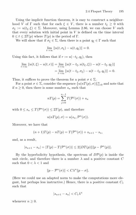
2.4 Floquet Theory 195
Using the implicit function theorem, it is easy to construct a neighbor-hood V of Γ such that for each ξ ∈ V , there is a number tξ ≥ 0 withσξ := u(tξ, ξ) ∈ Σ. Moreover, using Lemma 2.86, we can choose V suchthat every solution with initial point in V is defined on the time interval0 ≤ t ≤ 2T (p) where T (p) is the period of Γ.
We will show that if σξ ∈ Σ, then there is a point qξ ∈ Γ such that
limt→∞ ‖u(t, σξ) − u(t, qξ)‖ = 0.
Using this fact, it follows that if r := u(−tξ, qξ), then
limt→∞ ‖u(t, ξ) − u(t, r)‖ = lim
t→∞ ‖u(t − tξ, u(tξ, ξ)) − u(t − tξ, qξ)‖
= limt→∞ ‖u(t − tξ, σξ) − u(t − tξ, qξ)‖ = 0.
Thus, it suffices to prove the theorem for a point σ ∈ Σ.For a point σ ∈ Σ, consider the sequence u(nT (p), σ)∞
n=0 and note thatif n ≥ 0, then there is some number sn such that
nT (p) =n−1∑j=0
T (Pj(σ)) + sn
with 0 ≤ sn ≤ T (Pn(σ)) ≤ 2T (p), and therefore
u(nT (p), σ) = u(sn,Pn(σ)).
Moreover, we have that
(n + 1)T (p) − nT (p) = T (Pn(σ)) + sn+1 − sn,
and, as a result,
|sn+1 − sn| = |T (p) − T (Pn(σ))| ≤ 2‖DT (p)‖‖p − Pn(p)‖.
By the hyperbolicity hypothesis, the spectrum of DP(p) is inside theunit circle, and therefore there is a number λ and a positive constant Csuch that 0 < λ < 1 and
‖p − Pn(σ)‖ < Cλn‖p − σ‖.
(Here we could use an adapted norm to make the computations more ele-gant, but perhaps less instructive.) Hence, there is a positive constant C1such that
|sn+1 − sn| < C1λn
whenever n ≥ 0.
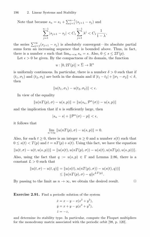
196 2. Linear Systems and Stability
Note that because sn = s1 +∑n−1
j=1 (sj+1 − sj) and
n−1∑j=1
|sj+1 − sj | < C1
n−1∑j=1
λj < C11
1 − λ,
the series∑∞
j=1(sj+1 − sj) is absolutely convergent—its absolute partialsums form an increasing sequence that is bounded above. Thus, in fact,there is a number s such that limn→∞ sn = s. Also, 0 ≤ s ≤ 2T (p).
Let ε > 0 be given. By the compactness of its domain, the function
u : [0, 2T (p)] × Σ → Rn
is uniformly continuous. In particular, there is a number δ > 0 such that if(t1, σ1) and (t2, σ2) are both in the domain and if |t1 − t2|+ ‖σ1 −σ2‖ < δ,then
‖u(t1, σ1) − u(t2, σ2)‖ < ε.
In view of the equality
‖u(nT (p), σ) − u(s, p)‖ = ‖u(sn,Pn(σ)) − u(s, p)‖
and the implication that if n is sufficiently large, then
|sn − s| + ‖Pn(σ) − p‖ < ε,
it follows that
limn→∞ ‖u(nT (p), σ) − u(s, p)‖ = 0.
Also, for each t ≥ 0, there is an integer n ≥ 0 and a number s(t) such that0 ≤ s(t) < T (p) and t = nT (p)+s(t). Using this fact, we have the equation
‖u(t, σ) − u(t, u(s, p))‖ = ‖u(s(t), u(nT (p), σ)) − u(s(t), u(nT (p), u(s, p))‖.
Also, using the fact that q := u(s, p) ∈ Γ and Lemma 2.86, there is aconstant L > 0 such that
‖u(t, σ) − u(t, q)‖ = ‖u(s(t), u(nT (p), σ)) − u(s(t), q))‖≤ ‖u(nT (p), σ) − q‖eLT (p).
By passing to the limit as n → ∞, we obtain the desired result.
Exercise 2.91. Find a periodic solution of the system
x = x − y − x(x2 + y2),
y = x + y − y(x2 + y2),
z = −z,
and determine its stability type. In particular, compute the Floquet multipliersfor the monodromy matrix associated with the periodic orbit [98, p. 120].
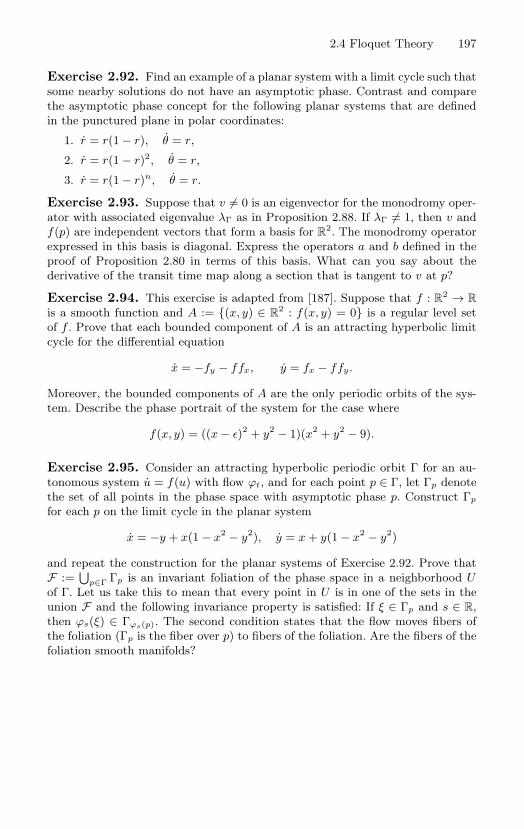
2.4 Floquet Theory 197
Exercise 2.92. Find an example of a planar system with a limit cycle such thatsome nearby solutions do not have an asymptotic phase. Contrast and comparethe asymptotic phase concept for the following planar systems that are definedin the punctured plane in polar coordinates:
1. r = r(1 − r), θ = r,
2. r = r(1 − r)2, θ = r,
3. r = r(1 − r)n, θ = r.
Exercise 2.93. Suppose that v = 0 is an eigenvector for the monodromy oper-ator with associated eigenvalue λΓ as in Proposition 2.88. If λΓ = 1, then v andf(p) are independent vectors that form a basis for R
2. The monodromy operatorexpressed in this basis is diagonal. Express the operators a and b defined in theproof of Proposition 2.80 in terms of this basis. What can you say about thederivative of the transit time map along a section that is tangent to v at p?
Exercise 2.94. This exercise is adapted from [187]. Suppose that f : R2 → R
is a smooth function and A := (x, y) ∈ R2 : f(x, y) = 0 is a regular level set
of f . Prove that each bounded component of A is an attracting hyperbolic limitcycle for the differential equation
x = −fy − ffx, y = fx − ffy.
Moreover, the bounded components of A are the only periodic orbits of the sys-tem. Describe the phase portrait of the system for the case where
f(x, y) = ((x − ε)2 + y2 − 1)(x2 + y2 − 9).
Exercise 2.95. Consider an attracting hyperbolic periodic orbit Γ for an au-tonomous system u = f(u) with flow ϕt, and for each point p ∈ Γ, let Γp denotethe set of all points in the phase space with asymptotic phase p. Construct Γp
for each p on the limit cycle in the planar system
x = −y + x(1 − x2 − y2), y = x + y(1 − x2 − y2)
and repeat the construction for the planar systems of Exercise 2.92. Prove thatF :=
⋃p∈Γ Γp is an invariant foliation of the phase space in a neighborhood U
of Γ. Let us take this to mean that every point in U is in one of the sets in theunion F and the following invariance property is satisfied: If ξ ∈ Γp and s ∈ R,then ϕs(ξ) ∈ Γϕs(p). The second condition states that the flow moves fibers ofthe foliation (Γp is the fiber over p) to fibers of the foliation. Are the fibers of thefoliation smooth manifolds?
3Applications
Is the subject of ordinary differential equations important? The ultimateanswer to this question is certainly beyond the scope of this book. However,two main points of evidence for an affirmative answer are provided in thischapter:
• Ordinary differential equations arise naturally from the foundationsof physical science.
• Ordinary differential equations are useful tools for solving physicalproblems.
You will have to decide if the evidence is sufficient. Warning: If you paytoo much attention to philosophical issues concerning the value of a math-ematical subject, then you might stop producing mathematics. However,if you pay no attention to the value of a subject, then how will you knowthat it is worthy of study?
3.1 Origins of ODE: The Euler–Lagrange Equation
Let us consider a smooth function L : Rk × R
k × R → R, a pair of pointsp1, p2 ∈ R
k, two real numbers t1 < t2, and the set C := C(p1, p2, t1, t2) ofall smooth curves q : R → R
k such that q(t1) = p1 and q(t2) = p2. Usingthis data, there is a function Φ : C → R given by
Φ(q) =∫ t2
t1
L(q(t), q(t), t) dt. (3.1)
200 3. Applications
The Euler–Lagrange equation, an ordinary differential equation associatedwith the function L—called the Lagrangian—arises from the followingproblem: Find the extreme points of the function Φ. This variational prob-lem is the basis for Lagrangian mechanics.
Recall from the calculus that an extreme point of a smooth functionis simply a point at which its derivative vanishes. To use this definitiondirectly for the function Φ, we would have to show that C is a manifoldand that Φ is differentiable. This can be done. However, we will bypassthese requirements by redefining the notion of extreme point. In effect, wewill define the concept of directional derivative for a scalar function on aspace of curves. Then, an extreme point is defined to be a point where alldirectional derivatives vanish.
Recall our geometric interpretation of the derivative of a smooth functionon a manifold: For a tangent vector at a point in the domain of the function,take a curve whose tangent at time t = 0 is the given vector, move the curveto the range of the function by composing it with the function and thendifferentiate the resulting curve at t = 0 to produce the tangent vector onthe range that is the image of the original vector under the derivative ofthe function. In the context of the function Φ on the space of curves C, letus consider a curve γ : R → C. Note that for s ∈ R, the point γ(s) ∈ Cis a curve γ(s) : R → R
k as defined above. So, in particular, if t ∈ R,then γ(s)(t) ∈ R
k. Rather than use the cumbersome notation γ(s)(t), it iscustomary to interpret our curve of curves as a “variation of curves” in C,that is, as a smooth function Q : R × R → R
k with the “end conditions”
Q(s, t1) ≡ p1, Q(s, t2) ≡ p2.
In this interpretation, γ(s)(t) = Q(s, t).Fix a point q ∈ C and suppose that γ(0) = q, or equivalently that
Q(0, t) = q(t). Then, as s varies we obtain a family of curves called avariation of the curve q. The tangent vector to γ at q is, by definition, thecurve V : R → R
k × Rk given by t → (q(t), v(t)) where
v(t) :=∂
∂sQ(s, t)
∣∣∣s=0
.
Of course, v is usually not in C because it does not satisfy the requiredend conditions. However, v does satisfy a perhaps different pair of endconditions, namely,
v(t1) =∂
∂sQ(s, t1)
∣∣∣s=0
= 0, v(t2) =∂
∂sQ(s, t2)
∣∣∣s=0
= 0.
Let us view the vector V as an element in the “tangent space of C at q.”
3.1 Origins of ODE: The Euler–Lagrange Equation 201
What is the directional derivative DΦ(q)V of Φ at q in the direction V ?Following the prescription given above, we have the definition
DΦ(q)V :=∂
∂sΦ(Q(s, t))
∣∣∣s=0
=∫ t2
t1
∂
∂sL(Q(s, t),
∂
∂tQ(s, t), t)
∣∣∣s=0
dt
=∫ t2
t1
(∂L
∂q
∂Q
∂s+
∂L
∂q
∂2Q
∂s∂t
)∣∣∣s=0
dt.
After evaluation at s = 0 and an integration by parts, we can rewrite thelast integral to obtain
DΦ(q)V =∫ t2
t1
[∂L
∂q(q(t), q(t), t) − d
dt
(∂L
∂q(q(t), q(t), t)
)]∂Q
∂s(0, t) dt
=∫ t2
t1
[∂L
∂q(q(t), q(t), t) − ∂
∂t
(∂L
∂q(q(t), q(t), t)
)]v(t) dt. (3.2)
If DΦ(q)V = 0 for all vectors V , then the curve q is called an extremal. Inother words, q is an extremal if the last integral in equation (3.2) vanishesfor all smooth functions v that vanish at the points t1 and t2.
Proposition 3.1. The curve q is an extremal if and only if it is a solutionof the Euler–Lagrange equation
d
dt
(∂L
∂q
)− ∂L
∂q= 0.
Proof. Clearly, if the curve q is a solution of the Euler–Lagrange equation,then, by formula (3.2), we have that DΦ(q) = 0. Conversely, if DΦ(q) = 0,we will show that q is a solution of the Euler–Lagrange equation. If not,then there is some time t1 < τ < t2 such that the quantity
∂L
∂q(q(τ), q(τ), τ) − ∂
∂t
(∂L
∂q(q(τ), q(τ), τ)
)appearing in the formula (3.2) does not vanish. In this case, this quantityhas constant sign on a closed interval containing the point τ . But there is asmooth nonnegative function v with support in this same interval such thatv(τ) = 1. It follows that for some corresponding variation, DΦ(q)V = 0, incontradiction.
When we search for the extreme points of functions we are usually inter-ested in the maxima or minima of the function. The same is true for thefunction Φ defined above. In fact, the theory for determining the maximaand minima of Φ is similar to the usual theory in finite dimensions, but
202 3. Applications
it is complicated by the technical problems of working in infinite dimen-sional spaces. The general theory is explained in books on the calculus ofvariations (see for example [61]).
In mechanics, the Lagrangian L is taken to be the difference between thekinetic energy and the potential energy of a particle, the function (3.1) iscalled the action, and a curve q : R → R
k is called a motion. Hamilton’sprinciple states: Every motion of a physical particle is an extremal of itsaction. Of course, the motions of a particle as predicted by Newton’s secondlaw are the same as the motions predicted by Hamilton’s principle (seeExercise 3.2).
Exercise 3.2. Prove: The motions of a particle determined by Newton’s secondlaw are the same as the motions determined by Hamilton’s principle. In thiscontext, Newton’s law states that the time rate of change of the momentum(mass×velocity) is equal to the negative gradient of the potential energy.
One beautiful feature of Lagrangian mechanics, which is evident fromthe definition of extremals, is the fact that Lagrangian mechanics is coor-dinate free. In particular, the form of the Euler–Lagrange equation doesnot depend on the choice of the coordinate system! Thus, if we want todescribe the motion of a particle, then we are free to choose the coordi-nates q := (q1, · · · , qk) as we please and still use the same form of theEuler–Lagrange equation.
As an illustration, consider the prototypical example in mechanics: a freeparticle. Let (x, y, z) denote the usual Cartesian coordinates in space andt → q(t) := (x(t), y(t), z(t)) the position of the particle as time evolves.The kinetic energy of a particle with mass m in Cartesian coordinates ism2 (x2(t) + y2(t) + z2(t)). Thus, the “action functional” is given by
Φ(q) =∫ t2
t1
m
2(x2(t) + y2(t) + z2(t)) dt,
the Euler–Lagrange equations are simply
mx = 0, my = 0, mz = 0, (3.3)
and each motion is along a straight line, as expected.As an example of the Euler–Lagrange equations in a non-Cartesian co-
ordinate system, let us consider the motion of a free particle in cylindri-cal coordinates (r, θ, z). To determine the Lagrangian, note that the ki-netic energy depends on the Euclidean structure of space, that is, on theusual inner product. A simple computation shows that the kinetic energyof the motion t → (r(t), θ(t), z(t)) expressed in cylindrical coordinates ism2 (r2(t) + r2θ2(t) + z2(t)). For example, to compute the inner product oftwo tangent vectors relative to a cylindrical coordinate chart, move them
3.2 Origins of ODE: Classical Physics 203
to the Cartesian coordinate chart by the derivative of the cylindrical co-ordinate wrapping function (Section 1.7.4), and then compute the usualinner product of their images. The Euler–Lagrange equations are
mr − mrθ2 = 0, md
dt(r2θ) = 0, mz = 0. (3.4)
Clearly, cylindrical coordinates are not the best choice to determine themotion of a free particle! But it does indeed turn out that all solutions ofsystem (3.4) lie on straight lines (see Exercise 3.3).
Exercise 3.3. Show that all solutions of system (3.4) lie on straight lines. Com-pare the parametrization of the solutions of system (3.4) with the solutions of thesystem (3.3). Hint: If necessary, read the next section, especially, the discussionon the integration of the equations of motion for a particle in a central forcefield—Kepler’s problem.
Exercise 3.4. Repeat Exercise 3.3 for spherical coordinates.
Exercise 3.5. Discuss the extremals for the function
Φ(q) =∫ t2
t1
(q21(t) + q2
2(t) + q23(t))1/2 dt.
3.2 Origins of ODE: Classical Physics
What is classical physics? Look at Section 18–2 in Richard Feynman’slecture notes [66] and you might be in for a surprise. The fundamental lawsof all of classical physics can be reduced to a few formulas! For example, acomplete theory of electromagnetics is given by Maxwell’s laws
div E = ρ/ε0,
curlE = −∂B∂t
,
div B = 0,
c2 curlB =jε0
+∂E∂t
and the conservation of charge
div(j) = −∂ρ
∂t.
Here E is the called electric field, B is the magnetic field, ρ is the chargedensity, j is the current, ε0 is a constant, and c is the speed of light. Thefundamental law of motion is Newton’s law
dpdt
= F
204 3. Applications
“the rate of change of the momentum is equal to the sum of the forces.”The (relativistic) momentum of a particle is given by
p :=m√
1 − v2/c2v
where, as is usual in the physics literature, v := |v| and the norm is theEuclidean norm. For a classical particle (velocity much less than the speedof light), the momentum is approximated by p = mv. There are two fun-damental forces: The gravitational force
F = −GMm
r2 er
on a particle of mass m due to a second mass M where G is the univer-sal gravitational constant and er is the unit vector at M pointing in thedirection of m; and the Lorentz force
F = q(E + v × B)
where q is the charge on a particle in an electromagnetic field. That’s it!The laws of classical physics seem simple enough. Why then is physics,
not to mention engineering, so complicated? Of course, the answer is thatin almost all real world applications there are lots of particles and thefundamental laws act all at once. When we try to isolate some experiment orsome physical phenomenon from all the other stuff in the universe, then weare led to develop “constitutive” laws that approximate the true situation.The equations of motion then contain many additional “forces.” Let usconsider a familiar example. When we model the motion of a spring, weuse Hooke’s force law to obtain the equation of motion in the form
mx = −ω0x.
However, Hooke’s force law is not one of the two fundamental force laws.In reality, the particles that constitute the spring obey the electromagneticforce law and the law of universal gravitation. However, if we attemptedto model the fundamental forces acting on each of these particles, then theequations of motion would be so complex that we would not be able toderive useful predictions.
What law of nature are we using when we add viscous damping to aHookian spring to obtain the differential equation
mx = −αx − ω0x
as a model? The damping term is supposed to model a force due to friction.But what is friction? There are only two fundamental forces in classicalphysics and only four known forces in modern physics. Friction is not a
3.2 Origins of ODE: Classical Physics 205
nuclear force and it is not due to gravitation. Thus, at a fundamental levelit must be a manifestation of electromagnetism. Is it possible to derive thelinear form of viscous damping from Maxwell’s laws? This discussion couldbecome very philosophical!
The important point for us is an appreciation that the law of motion—sobasic for our understanding of the way the universe works—is expressed asan ordinary differential equation. Newton’s law, the classical force laws,and the constitutive laws are the origin of ordinary differential equations.Apparently, as Newton said, “Solving differential equations is useful.”
In the following subsections some applications of the theory of differentialequations to problems that arise in classical physics are presented. The firstsection briefly describes the motion of a charged particle in a constant elec-tromagnetic field. The second section is an introduction to the two-bodyproblem, including Kepler motion, Delaunay elements, and perturbationforces. The analysis of two-body motion is used as a vehicle to explore arealistic important physical problem where it is not at all obvious how toobtain useful predictions from the complicated model system of differentialequations obtained from Newton’s law. Perturbations of two-body motionare considered in the final sections: Satellite motion about an oblate planetis used to illustrate the “method of averaging,” and the diamagnetic Keplerproblem—the motion of an electron of a hydrogen atom in a constant mag-netic field—is used to illustrate some important transformation methodsfor the analysis of models of mechanical systems.
3.2.1 Motion of a Charged ParticleLet us consider a few simple exercises to “feel” the Lorentz force (for moresee [66] and [104]). The equation of motion for a charged particle is
dpdt
= q(E + v × B)
where p is the momentum vector, q is a measure of the charge, and v is thevelocity. For this section let us consider only the case where the electric fieldE and the magnetic field B are constant vector fields on R
3. The problemis to determine the motion of a charged particle (classical and relativistic)in case B = 0 and, also, in case E = 0.
In case E = 0, let us consider the relativistic motion for a charged par-ticle. Because the momentum is a nonlinear function of the velocity, it isuseful to notice that the motion is “integrable.” In fact, the two functionsp → 〈p,p〉 and p → 〈p,B〉 are constant along orbits. Use this fact toconclude that v → 〈v,v〉 is constant along orbits, and therefore the energy
E :=mc2√
1 − v2/c2
206 3. Applications
is constant along orbits. It follows that the equation of motion can be recastin the form
Ec2 v = qv × B,
and the solution can be found as in Exercise 2.30. The solution of thisdifferential equation is important. For example, the solution can be used toplace magnetic fields in an experiment so that charged particles are movedto a detector (see [66]). What can you say about the motion of a chargedparticle if both electric and magnetic fields are present?
Exercise 3.6. Use the theory of linear differential equations with constant co-efficients to determine the motion for a “spatial oscillator” (see [104]) in thepresence of a constant magnetic field. The equation of motion is
v = −ω20r +
q
mv × B
where r = (x, y, z) is the position vector, the velocity is v = (x, y, z), and B =(0, 0, B3). (This model uses Hooke’s law). By rewriting the equations of motionin components, note that this model is a linear system with constant coefficients.Find the general solution of the system. Determine the frequency of the motion inthe plane perpendicular to the magnetic field and the frequency in the directionof the magnetic field.
3.2.2 Motion of a Binary SystemLet us consider two point masses, m1 and m2, moving in three-dimensionalEuclidean space with corresponding position vectors R1 and R2. Also, letus define the relative position vector R := R2 − R1 and its length r := |R|.According to Newton’s law (using of course the usual approximation forsmall velocities) and the gravitational force law, we have the equations ofmotion
m1R1 =G0m1m2
r3 R + F1, m2R2 = −G0m1m2
r3 R + F2
where F1 and F2 are additional forces acting on m1 and m2 respectively.The relative motion of the masses is governed by the single vector equation
R = −G0(m1 + m2)r3 R +
1m2
F2 − 1m1
F1.
By rescaling distance and time such that R = αR and t = βt withG0(m1 +m2)β2 = α3, we can recast the equations of motion in the simplerform
R = − 1r3 R + F. (3.5)
3.2 Origins of ODE: Classical Physics 207
We will study this differential equation.The analysis of two-body interaction plays a central role in the history
of science. This is reason enough to study the dynamics of the differentialequation (3.5) and the surrounding mathematical terrain. However, as youwill see, the intrinsic beauty, rich texture, and wide applicability of thissubject make it one of the most absorbing topics in all of mathematics.
The following glimpse into celestial mechanics is intended to introducean important application of ordinary differential equations, to see some ofthe complexity of a real world application and to introduce a special form ofthe dynamical equations that will provide some motivation for the theoryof averaging presented in Chapter 7.
There are many different approaches to celestial mechanics. However,for a mathematician, the most satisfactory foundation for mechanics isprovided by the theory of Hamiltonian systems. While we will use Hamil-ton’s equations in our analysis, the geometric context (symplectic geome-try) for a modern treatment of the transformation theory for Hamiltoniansystems (see [1], [10], and [123]) is unfortunately beyond the scope of thisbook. To bypass this theory, we will present an expanded explanation ofthe direct change of coordinates to the Delaunay elements given in [45](see also [41] and [44]). In the transformation theory for Hamiltonian sys-tems it is proved that our transformations are special coordinate transfor-mations called canonical transformations. They have a special property:Hamilton’s equations for the transformed Hamiltonian are exactly the dif-ferential equations given by the push forward of the original Hamiltonianvector field to the new coordinates. In other words, to perform a canonicalchange of coordinates we need only transform the Hamiltonian, not the dif-ferential equations; the transformed differential equations are obtained bycomputing Hamilton’s equations from the transformed Hamiltonian. Thedirect method is perhaps not as elegant as the canonical transformationapproach—we will simply push forward the Hamiltonian vector field in theusual way—but the direct transformation method is effective and useful.Indeed, we will construct special coordinates (action-angle coordinates) andshow that they transform the Kepler system to a very simple form. More-over, the direct method applies even if a nonconservative force F acts onthe system; that is, even if the equations of motion are not Hamiltonian.
Let us begin by rewriting the second order differential equation (3.5) asthe first order system
R = V, V = − 1r3 R + F (3.6)
defined on R3×R
3. Also, let us use angle brackets to denote the usual innerproduct on R
3 so that if X ∈ R3, then |X|2 = 〈X, X〉.
The most important feature of system (3.6) is the existence of conservedquantities for the Kepler motion, that is, the motion with F = 0. In fact,total energy and angular momentum are conserved. The total energy of the
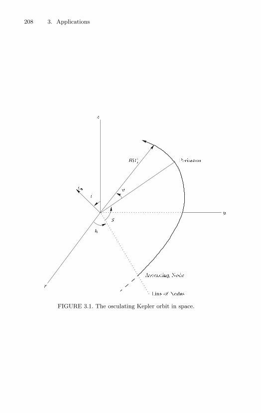
208 3. Applications
x
z
Line of Nodes
Ascending Node
Periaston
y
g
h
i
ven
Rt
FIGURE 3.1. The osculating Kepler orbit in space.
3.2 Origins of ODE: Classical Physics 209
Kepler motion E : R3 × R
3 → R is given by
E(X, Y ) :=12〈Y, Y 〉 − 1
〈X, X〉1/2 , (3.7)
the angular momentum by
A(X, Y ) := X × Y. (3.8)
Let us also define the total angular momentum
G(X, Y ) := |A(X, Y )|. (3.9)
Note that we are using the term “angular momentum” in a nonstandardmanner. In effect, we have defined the angular momentum to be the vec-tor product of position and velocity ; in physics, angular momentum is thevector product of position and momentum.
If t → (R(t), V (t)) is a solution of system (3.6), then
E =d
dtE(R(t), V (t)) = 〈F, V 〉, A = R × F. (3.10)
Thus, if F = 0, then E and A are constant on the corresponding orbit.In particular, in this case the projection of the Kepler orbit into physicalspace, corresponding to the curve t → R(t), is contained in a fixed planepassing through the origin with normal vector given by the constant valueof A along the orbit. In this case, the corresponding plane normal to A iscalled the osculating plane. At each instant of time, this plane contains theKepler orbit that would result if the force F were not present thereafter.Refer to Figure 3.1 for a depiction of the curve t → R(t) in space and theangles associated with the Delaunay elements.
Let us define three functions er : R3 → R
3, and eb, en : R3 ×R
3 → R3 by
er(X) =1
|X|X,
en(X, Y ) =1
G(X, Y )X × Y,
eb(X, Y ) = en(X, Y ) × er(X, Y ).
If X, Y ∈ R3 are distinct nonzero points, then the vectors er(X), eb(X, Y ),
and en(X, Y ) form an orthonormal frame in R3. Also, if these functions are
evaluated along the (perturbed) solution t → (R, R), then we have
er =1rR, en =
1G
R × R, eb =1
rG(R × R) × R =
1rG
(r2R − 〈R, R〉R).
(3.11)
210 3. Applications
(Note that subscripts are used in this section to denote coordinate direc-tions, not partial derivatives.)
If ex, ey, ez are the direction vectors for a fixed right-handed usual Carte-sian coordinate system in R
3, and if i denotes the inclination angle of theosculating plane relative to the z-axis, then
cos i = 〈en, ez〉. (3.12)
Of course, the angle i can also be viewed as a function on R3 × R
3 whosevalue at each point on the orbit is the inclination of the osculating plane.The idea is that we are defining new variables: They are all functions definedon R
3 × R3.
If the osculating plane is not coincident with the (x, y)-plane, then itmeets this plane in a line, called the line of nodes. Of course, the line ofnodes lies in the osculating plane and is orthogonal to the z-axis. Moreover,it is generated by the vector
ean := 〈eb, ez〉er − 〈er, ez〉eb.
The angle of the ascending node h between the x-axis and the line of nodesis given by
cos h =1
|ean| 〈ean, ex〉. (3.13)
If the osculating plane happens to coincide with the (x, y)-plane, then thereis no natural definition of h. However, on an orbit the angle h(t) is contin-uous. At a point where i(t) = π/2, the angle h is defined whenever there isa continuous extension.
Let us compute the orthogonal transformation relative to the Euler an-gles i and h. This is accomplished in two steps: rotation about the z-axisthrough the angle h followed by rotation about the now rotated x-axisthrough the angle i. The rotation matrix about the z-axis is
M(h) :=
cos h − sin h 0sin h cos h 0
0 0 1
.
To rotate about the new x-axis (after rotation by M(h)), let us rotate backto the original coordinates, rotate about the old x-axis through the anglei, and then rotate forward. The rotation about the x-axis is given by
M(i) :=
1 0 00 cos i − sin i0 sin i cos i
.
Thus, the required rotation is
M := (M(h)M(i)M−1(h))M(h) = M(h)M(i).
3.2 Origins of ODE: Classical Physics 211
In components, if the new Cartesian coordinates are denoted x′, y′, z′, thenthe transformation M is given by
x = x′ cos h − y′ sin h cos i + z′ sin h sin i,
y = x′ sin h + y′ cos h cos i − z′ cos h sin i,
z = y′ sin i + z′ cos i. (3.14)
Also, by the construction, the normal en to the osculating plane is in thedirection of the z′-axis.
If polar coordinates are introduced in the osculating plane
x′ = r cos θ, y′ = r sin θ,
then the position vector along our orbit in the osculating coordinates isgiven by
R(t) = (r(t) cos θ(t), r(t) sin θ(t), 0).
For a Kepler orbit, the osculating plane is fixed. Also, using the orthog-onal transformation M , the vectors R and R are given in the original fixedcoordinates by
R = M
r cos θr sin θ
0
, R = M
r cos θ − rθ sin θ
r sin θ + rθ cos θ0
. (3.15)
If X, Y ∈ R3, then, because M is orthogonal, we have 〈MX, MY 〉 = 〈X, Y 〉.
As a consequence of this fact and definition (3.7), it follows that the totalenergy along the orbit is
E(R, R) =12(r2 + r2θ2) − 1
r.
Also, using the coordinate-free definition of the vector product,
X × Y := (|X||Y | sin θ)η (3.16)
where η is the unit vector orthogonal to X and Y such that the orderedtriple (X, Y, η) has positive (right hand) orientation, and the fact that Mpreserves positive orientation (det M > 0); it follows that MX × MY =X × Y and the angular momentum along the orbit is
A(R, R) = r2θ. (3.17)
Thus, using equation (3.10), there is a constant (angular momentum) Pθ
such that
r2θ = Pθ, E =12(r2 +
P 2θ
r2
)− 1
r, (3.18)
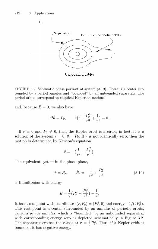
212 3. Applications
Pr
SeparatrixBounded periodic orbits
Unbounded orbits
r
FIGURE 3.2. Schematic phase portrait of system (3.19). There is a center sur-rounded by a period annulus and “bounded” by an unbounded separatrix. Theperiod orbits correspond to elliptical Keplerian motions.
and, because E = 0, we also have
r2θ = Pθ, r(r − P 2
θ
r3 +1r
)= 0.
If r ≡ 0 and Pθ = 0, then the Kepler orbit is a circle; in fact, it is asolution of the system r = 0, θ = Pθ. If r is not identically zero, then themotion is determined by Newton’s equation
r = −( 1r2 − P 2
θ
r3
).
The equivalent system in the phase plane,
r = Pr, Pr = − 1r2 +
P 2θ
r3 (3.19)
is Hamiltonian with energy
E =12(P 2
r +P 2
θ
r2
)− 1
r.
It has a rest point with coordinates (r, Pr) = (P 2θ , 0) and energy −1/(2P 2
θ ).This rest point is a center surrounded by an annulus of periodic orbits,called a period annulus, which is “bounded” by an unbounded separatrixwith corresponding energy zero as depicted schematically in Figure 3.2.The separatrix crosses the r-axis at r = 1
2P 2θ . Thus, if a Kepler orbit is
bounded, it has negative energy.
3.2 Origins of ODE: Classical Physics 213
Exercise 3.7. Prove all of the statements made about the phase portrait ofsystem (3.19).
Exercise 3.8. The vector product is defined in display (3.16) in a coordinate-free manner. Suppose instead that X = (x1, x2, x3) and Y = (y1, y2, y3) in Carte-sian coordinates, and their cross product is defined to be
X × Y := det
e1 e2 e3
x1 x2 x3
y1 y2 y3
.
Discuss the relative utility of the coordinate-free versus coordinate-dependentdefinitions. Determine the vector product for vectors expressed in cylindrical orspherical coordinates. Think about the concept of coordinate free-definitions; itis important!
The rest of the discussion is restricted to orbits with negative energy andpositive angular momentum Pθ > 0.
The full set of differential equations for the Kepler motion is the firstorder system
r = Pr, θ =Pθ
r2 , Pr =1r2
(P 2θ
r− 1
), Pθ = 0. (3.20)
Note that the angle θ increases along orbits because θ = Pθ/r2 > 0. Also,the bounded Kepler orbits project to periodic motions in the r–Pr phaseplane. Thus, the bounded orbits can be described by two angles: the polarangle relative to the r-axis in the r–Pr plane and the angular variable θ.In other words, each bounded orbit lies on the (topological) cross productof two circles; that is, on a two-dimensional torus. The fact that the phasespace for the Kepler motion is foliated by invariant two-dimensional tori isthe underlying reason why we will eventually be able to define special coor-dinates, called action-angle coordinates, that transform the Kepler systemto a very simple form. In fact, the special class of Hamiltonian systems(called integrable Hamiltonian systems) that have a portion of their phasespace foliated by invariant tori can all be transformed to a simple formby the introduction of action-angle coordinates. The construction uses thefact that the motion on each invariant torus is periodic or quasi-periodicwhere the frequencies vary with the choice of the torus. This is exactly theunderlying idea for the construction of the action-angle coordinates for theKepler system.
To integrate system (3.20), introduce a new variable ρ = 1/r so that
ρ = −ρ2Pr, Pr = ρ2(ρP 2θ − 1),
and then use θ as a time-like variable to obtain the linear system
dρ
dθ= − 1
PθPr,
dPr
dθ=
1Pθ
(ρP 2θ − 1). (3.21)
214 3. Applications
Equivalently, we have the “harmonic oscillator model” for Kepler motion,
d2ρ
dθ2 + ρ =1
P 2θ
. (3.22)
It has the general solution
ρ =1
P 2θ
+ B cos(θ − g) (3.23)
where the numbers B and g are determined by the initial conditions.The Kepler orbit is an ellipse. In fact, by a rearrangement of equa-
tion (3.23) we have
r =P 2
θ
1 + P 2θ B cos(θ − g)
.
If we introduce a new angle, the true anomaly v := θ − g, and the usualquantities—the eccentricity e, and a, the semimajor axis of the ellipse—then
r =a(1 − e2)1 + e cos v
. (3.24)
Exercise 3.9. Use the conservation of energy for system (3.20) to show that
dr
dθ=
r
Pθ
(2Er2 + 2r − P 2
θ
)1/2.
Solve this differential equation for E < 0 and show that the Kepler orbit is anellipse.
Using the fact that the energy is constant on the Kepler orbit, if wecompute the energy at v = 0 (corresponding to its perifocus, the point onthe ellipse closest to the focus), we have the corresponding values
r = a(1 − e), r = 0, E = − 12a
. (3.25)
Moreover, from the usual theory of conic sections, the semiminor axis isb = a
√1 − e2, and the area of the ellipse is
πab = πa2√
1 − e2 = πPθa3/2. (3.26)
Taking into account the fact that the area element in polar coordinates is12ρ2 dθ, if the period of the Kepler orbit is T , then∫ T
0
r2(θ)2
dθ = πPθa3/2.
3.2 Origins of ODE: Classical Physics 215
Because r2θ = Pθ, the integral can be evaluated. The resulting equation isKepler’s third law
T 2 = 4π2a3 (3.27)
where, again, T is the orbital period and a is the semimajor axis of thecorresponding elliptical orbit. For later reference, note that the frequencyof the oscillation is
ω :=1
a3/2 . (3.28)
Exercise 3.10. Kepler’s third law is given by equation (3.27) for scaled dis-tance and time. Show that Kepler’s third law in “unscaled” variables (with thesame names as in (3.27)) is given by
T 2 =4π2
G0(m1 + m2)a3.
Also, show that the magnitude of the physical angular momentum in the unscaledvariables for a Kepler orbit is
m2r2θ =
(α3
β2 a(1 − e2))1/2 =
(G0(m1 + m2)a(1 − e2)
)1/2.
3.2.3 Disturbed Kepler Motion and Delaunay ElementsIn this section we will begin an analysis of the influence of a force F ona Keplerian orbit by introducing new variables, called Delaunay elements,such that system (3.5) when recast in the new coordinates has a usefulspecial form given below in display (3.52).
Recall the orthonormal frame [er, eb, en] in display (3.11), and let
F = Frer + Fbeθ + Fnen.
The functions L, G : R3 × R
3 → R, two of the components of the Delaunaycoordinate transformation, are defined by
L(X, Y ) := (−2E(X, Y ))−1/2, G(X, Y ) := |A(X, Y )|
where E is the energy and A the angular momentum. Using the results indisplay (3.10), we have that
L = L3〈F, R〉, G =1G
〈R × R, F × R〉.
Moreover, in view of the vector identities
〈α, β × γ〉 = 〈γ, α × β〉 = 〈β, γ × α〉,(α × β) × γ = 〈γ, α〉β − 〈γ, β〉α,
216 3. Applications
and the results in display (3.11), it follows that
G =1G
〈F, (R × R) × R〉 =1G
〈F, rGeb〉 = rFb. (3.29)
Also, using the formula for the triple vector product and the equality rr =〈R, R〉, which is obtained by differentiating both sides of the identity r2 =〈R,R〉, we have
eb =1
rG(R × R) × R =
1rG
(r2R − 〈R, R〉R)
and
R = rer +G
reb. (3.30)
As a result, the Delaunay elements L and G satisfy the differential equations
L = L3(rFr +G
rFb), G = rFb. (3.31)
If the force F does not vanish, then the relations found previously for thevariables related to the osculating plane of the Kepler orbit are still valid,only now the quantities a, e, v, and Pθ > 0 all depend on time. Thus, forexample, if we use equation (3.17), then
G = Pθ =√
a(1 − e2). (3.32)
Also, from equations (3.25), (3.30), and the definition of L we have
L =√
a, e2 = 1 − G2
L2 , (3.33)
and
− 12a
=12〈R, R〉 − 1
r=
12(r2 +
a(1 − e2)r2
)− 1
r. (3.34)
Let us solve for r2 in equation (3.34), express the solution in the form
r2 = − 1ar2 (r − a(1 − e))(r − a(1 + e)),
and substitute for r from formula (3.24) to obtain
r =e sin v
G. (3.35)
Hence, from equation (3.31),
L = L3(Fre
Gsin v + Fb
G
r
), G = rFb. (3.36)
3.2 Origins of ODE: Classical Physics 217
The Delaunay variable H is defined by
H := 〈A, ez〉 = G〈 1G
R × R, ez〉 = G cos i (3.37)
where i is the inclination angle of the osculating plane (see equation (3.12)).To find an expression for H, let us first recall the transformation equa-tions (3.14). Because en has “primed” coordinates (0, 0, 1), it follows thaten has original Cartesian coordinates
en = (sinh sin i,− cos h sin i, cos i), (3.38)
and, similarly, R is given by
R = r(cos θ cos h − sin θ sin h cos i, cos θ sin h + sin θ cos h cos i, sin θ sin i).(3.39)
Using equation (3.38) and equation (3.39), we have
eb = en × er
=1ren × R
= (− sin θ cos h − cos θ sin h cos i,
− sin θ sin h + cos θ cos h cos i, cos θ sin i). (3.40)
If we now differentiate both sides of the identity Gen = A, use the fact thater × eθ = en, and use the second identity of display (3.10), then
Gen = A − Gen
= rer × F − rFben
= r(Fber × eb − Fner × en) − rFben
= −rFneθ. (3.41)
The equations
di
dt=
rFn
Gcos θ, h =
rFn sin θ
G sin i(3.42)
are found by equating the components of the vectors obtained by sub-stitution of the identities (3.38) and (3.40) into (3.41). Finally, using thedefinition (3.37) together with equations (3.36) and (3.42), we have thedesired expression for the time derivative of H, namely,
H = r(Fb cos i − Fn sin i cos θ). (3.43)
Using the formula for R given in equation (3.30), the identity 〈er, ez〉 =sin θ sin i derived from equation (3.39), and the equation 〈eb, ez〉 = cos θ sin ifrom (3.40), let us note that
〈R, ez〉 = r sin i sin θ +G
rsin i cos θ.
218 3. Applications
A similar expression for 〈R, ez〉 is obtained by differentiation of both sidesof the last equation in display (3.14) and substitution for di/dt from (3.42).The following formula for θ is found by equating these two expressions:
θ =G
r2 − rFn cos i sin θ
G sin i. (3.44)
From equations (3.24) and (3.32),
r =G2
1 + e cos v. (3.45)
Let us solve for v in the equation obtained by logarithmic differentiation ofequation (3.45). Also, if we use the identity 1 − e2 = G2/L2 to find an ex-pression for e, substitute for L and G using the equation in display (3.36),and substitute for r using (3.35), then, after some simple algebraic manip-ulations,
v =G
r2 + FrG
ecos v + Fb
G2
re sin v
(G cos v
e− 2r
G− r2 cos v
eL2G
).
A more useful expression for v is obtained by substituting for r from equa-tion (3.45) to obtain
v =G
r2 + FrG
ecos v − Fb
G
e
(1 +
r
G2
)sin v. (3.46)
Recall equation (3.23), and define g, the argument of periastron, by g :=θ − v. Using equations (3.44) and (3.46), the time derivative g is
g = −FrG
ecos v + Fb
G
e
(1 +
r
G2
)sin v − Fn
r cos i
G sin isin(g + v). (3.47)
The last Delaunay element, , called the mean anomaly, is defined withthe aid of an auxiliary angle u, the eccentric anomaly, via Kepler’s equation
= u − e sin u (3.48)
where u is the unique angle such that
cos u =e + cos v
1 + e cos v, sin u =
1 − e cos u√1 − e2
sin v. (3.49)
The lengthy algebraic computations required to obtain a useful expres-sion for are carried out as follows: Differentiate both sides of Kepler’sequation and solve for in terms of u and e. Use the relations (3.49) andequation (3.45) to prove the identity
r = L2(1 − e cos u) (3.50)
3.2 Origins of ODE: Classical Physics 219
and use this identity to find an expression for u. After substitution usingthe previously obtained expressions for r, e, and L, it is possible to showthat
=1L3 +
r
eL
[(−2e + cos v + e cos2 v)Fr − (2 + e cos v) sin vFb
]. (3.51)
In summary, the Delaunay elements (L, G, H, , g, h) for a Keplerian mo-tion disturbed by a force F satisfy the following system of differential equa-tions:
L = L3(Fre
Gsin v + Fb
G
r
),
G = rFb,
H = r(Fb cos i − Fn sin i cos(g + v)),
=1L3 +
r
eL
[(−2e + cos v + e cos2 v)Fr − (2 + e cos v) sin vFb
],
g = −FrG
ecos v + Fb
G
e
(1 +
r
G2
)sin v − Fn
r cos i
G sin isin(g + v),
h = rFnsin(g + v)
G sin i. (3.52)
Our transformation of the equations of motion for the perturbed Keplerproblem to Delaunay elements—encoded in the differential equations indisplay (3.52)—is evidently not complete. Indeed, the components of theforce F , as well as the functions
r, e, cos v, sin v, cos i, sin i,
must be expressed in Delaunay elements. However, assuming that this isdone, it is still not at all clear how to extract useful information fromsystem (3.52). Only one fact seems immediately apparent: If the force F isnot present, then the Kepler motion relative to the Delaunay elements is asolution of the integrable system
L = 0, G = 0, H = 0, =1L3 , g = 0, h = 0.
In fact, by inspection of this unperturbed system, it is clear that the Ke-plerian motion is very simple to describe in Delaunay coordinates: Thethree “action” variables L, G, and H remain constant and only one of theangular variables, namely , is not constant. In particular, for each initialcondition, the motion is confined to a topological circle and corresponds touniform rotation of the variable , that is, simple harmonic motion. Thecorresponding Keplerian orbit is periodic.
The fact that two of the three angles that appear in system (3.52) remainconstant for unperturbed motions is a special, perhaps magical, feature
220 3. Applications
of the inverse square central force law. This special degeneracy of Keplermotion will eventually allow us to derive some rigorous results about theperturbed system, at least in the case where the force F is “small,” thatis, where F = εF, the function F is bounded, and ε ∈ R is regarded as asmall parameter.
As we have just seen, a suitable change of coordinates can be used totransform the Kepler model equations to a very simple form. The underly-ing reason, mentioned previously, is that a region in the unperturbed phasespace is foliated by invariant tori. Due to the special nature of the inversesquare force law, each two-dimensional torus in this foliation is itself foli-ated by periodic orbits, that is, by one-dimensional tori. In other words,there is an open region of the unperturbed phase space filled with periodicorbits.
In general, if there is a foliation by invariant two-dimensional tori, thenwe would expect the phase flow to be quasi-periodic on “most” of them—cut the flow with a Poincare section, in this case a one-dimensional torus,and suppose that the associated Poincare map is given by a linear rota-tion through an irrational angle. The remaining invariant tori would haveperiodic flow. Note that in this scenario where the Poincare map is eithera rational or an irrational rotation, the set of “quasi-periodic tori” andthe set of “periodic tori” are both dense. But, with respect to Lebesguemeasure, the set of quasi-periodic tori is larger. In fact, the set of quasi-periodic tori has measure one, whereas the set of periodic tori has measurezero. However, for the Kepler motion the flow is periodic on every torus.
The origin of many important questions in the subject of differentialequations arises from the problem of analyzing perturbations of integrablesystems; that is, systems whose phase spaces are foliated by invariant tori.In fact, if the phase space of a system is foliated by k-dimensional tori,then there is a new coordinate system in which the equations of motionhave the form
I = εP (I, φ), φ = Ω(I) + εQ(I, φ)
where I is a vector of “action variables,” θ is a k-dimensional vector of“angle variables,” and both P and Q are 2π-periodic functions of the an-gles. Poincare called the analysis of this system the fundamental problemof dynamics. In other words, if we start with a “completely integrable”mechanical system in action-angle variables so that it has the form I = 0,θ = Ω(I), and if we add a small force, then the problem is to describethe subsequent motion. This problem has been a central theme in mathe-matical research for over 100 years; it is still a prime source of importantproblems.
Let us outline a procedure to complete the transformation of the per-turbed Kepler system (3.52) to Delaunay elements. Use equation (3.32) and
3.2 Origins of ODE: Classical Physics 221
the definition of L to obtain the formula
G2 = L2(1 − e2),
and note that from the definition of H we have the identity
cos i =H
G.
From our assumption that G = Pθ > 0, and the fact that 0 ≤ i < π, we cansolve for e and i in terms of the Delaunay variables. Then, all the remainingexpressions not yet transformed to Delaunay variables in system (3.52) aregiven by combinations of terms of the form rn sin mv and rn cos mv wheren and m are integers. In theory we can use Kepler’s equation to solve foru as a function of and e. Thus, if we invert the transformation (3.49) andalso use equation (3.50), then we can express our combinations of r andthe trigonometric functions of v in Delaunay variables.
The inversion of Kepler’s equation is an essential element of the transfor-mation to Delaunay variables. At a more fundamental level, the inversionof Kepler’s equation is required to find the position of a planet on its el-liptical orbit as a function of time. The rigorous treatment of the inversionproblem seems to have played a very important role in the history of 19thcentury mathematics.
Problem 3.11. Write a report on the history and the mathematics relatedto Kepler’s equation. Include an account of the history of the theory of Besselfunctions ([52], [180]) and complex analysis ([13], [26]).
To invert Kepler’s equation formally, set w := u − so that
w = e sin(w + ),
suppose that
w =∞∑
j=1
wjej ,
use the sum formula for the sine, and equate coefficients in Kepler’s equa-tion for w to obtain the wj as trigonometric functions of . One method thatcan be used to make this inversion rigorous, the method used in Bessel’soriginal treatment, is to expand in Fourier series.
It is easy to see, by an analysis of Kepler’s equation, that the angle isan odd function of u. Thus, after inverting, u is an odd function of as ise sin u. Thus,
e sin u =2π
∞∑ν=1
(∫ π
0e sin u sin ν d
)sin ν,
222 3. Applications
and, after integration by parts,
e sin u =2π
∞∑ν=1
(1ν
∫ π
0cos ν(e cos u
du
d) d
)sin ν.
By Kepler’s equation e cos u = 1 − d/du. Also, we have that
e sin u =2π
∞∑ν=1
(1ν
∫ π
0cos(ν(u − e sin u)) du
)sin ν.
Bessel defined the Bessel function of the first kind
Jν(x) :=12π
∫ 2π
0cos(νs − x sin s) ds =
1π
∫ π
0cos(νs − x sin s) ds
so that
e sin u =∞∑
ν=1
2ν
Jν(νe) sin ν.
Hence, if we use the definition of the Bessel function and Kepler’s equation,then
u = +∞∑
ν=1
2ν
Jν(νe) sin ν.
By similar, but increasingly more difficult calculations, all products of theform
rn sin mu, rn cos mu, rn sin mv, rn cos mv,
where n and m are integers, can be expanded in Fourier series in whoseνth coefficients are expressed as linear combinations of Jν(νe) and J ′
ν(νe)(see [102] and [180]). Thus, we have at least one method to transformsystem (3.52) to Delaunay elements.
3.2.4 Satellite Orbiting an Oblate PlanetLet us consider a perturbation problem that arises from the fact that theshape of the earth is not a perfect sphere. The law of universal gravita-tion states that two particles (point masses) attract by the inverse squarelaw. The earth is composed of lots of particles. However, if the earth isidealized as a sphere with uniformly distributed mass, then the gravita-tional force exerted on a satellite obeys the inverse square law for the earthconsidered as a point mass concentrated at the center of the sphere. Butbecause the true shape of the earth is approximated by an oblate spheroid
3.2 Origins of ODE: Classical Physics 223
that “bulges” at the equator, the gravitational force exerted on a satellitedepends on the position of the satellite relative to the equator. As we willsee, the equations of motion of an earth satellite that take into account theoblateness of the earth are quite complex. At first sight it will probably notbe at all clear how to derive useful predictions from the model. However,as an illustration of some of the ideas introduced so far in this chapter, wewill see how to transform the model equations into action-angle variables.Classical perturbation theory can then be used to make predictions.
Introduce Cartesian coordinates so that the origin is at the center ofmass of an idealized planet viewed as an axially symmetric oblate spheroidwhose axis of symmetry is the z-axis. The “multipole” approximation ofthe corresponding gravitational potential has the form
−G0m1
r+ U(r, z) + O
((R0
r
)3)where
U = −12
G0m1J2R20
r3
(1 − 3
z2
r2
),
m1 is the mass of the planet, R0 is the equatorial radius, and J2 is aconstant related to the moments of inertia of the planet (see [72] and [118]).Note that the first term of the multipole expansion is just the point massgravitational law that determines the Kepler motion.
The oblateness problem has been widely studied by many different meth-ods, some more direct than our Delaunay variable approach (see [118], [142],[72], and [157]). However, our approach serves to illustrate some generalmethods that are widely applicable.
As an approximation to the gravitational potential, let us drop the higherorder terms and consider Kepler motion perturbed by the force determinedby the second term of the multipole expansion, that is, the perturbing forceper unit of mass is the negative gradient of U . Thus, in our notation, if welet m2 denote the mass of the satellite, then F2 = −m2 gradU and theequation of relative motion is given by
R = −G0(m1 + m2)r3 R − gradU. (3.53)
Of course, since the mass of the satellite is negligible relative to the massof the planet, the relative motion is essentially the same as the motion ofthe satellite.
To use the general formulas for transformation to Delaunay variablesgiven in display (3.52), we must first rescale system (3.53). For this, let βdenote a constant measured in seconds and let α := (G0(m1 +m2))1/3β2/3,so that α is measured in meters. Then, rescaling as in the derivation ofequation (3.5), we obtain the equation of motion
R = − 1r3 + F (3.54)
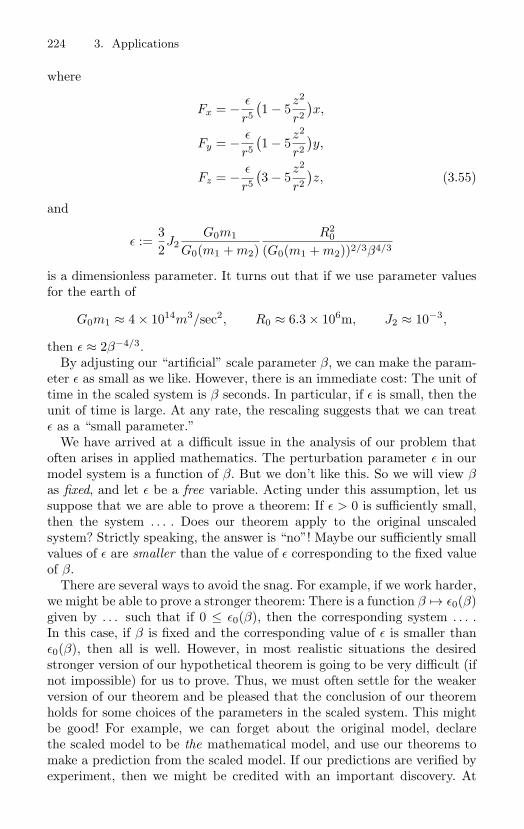
224 3. Applications
where
Fx = − ε
r5
(1 − 5
z2
r2
)x,
Fy = − ε
r5
(1 − 5
z2
r2
)y,
Fz = − ε
r5
(3 − 5
z2
r2
)z, (3.55)
and
ε :=32J2
G0m1
G0(m1 + m2)R2
0
(G0(m1 + m2))2/3β4/3
is a dimensionless parameter. It turns out that if we use parameter valuesfor the earth of
G0m1 ≈ 4 × 10¹⁴m3/sec2, R0 ≈ 6.3 × 10⁶m, J2 ≈ 10−3,
then ε ≈ 2β−4/3.By adjusting our “artificial” scale parameter β, we can make the param-
eter ε as small as we like. However, there is an immediate cost: The unit oftime in the scaled system is β seconds. In particular, if ε is small, then theunit of time is large. At any rate, the rescaling suggests that we can treatε as a “small parameter.”
We have arrived at a difficult issue in the analysis of our problem thatoften arises in applied mathematics. The perturbation parameter ε in ourmodel system is a function of β. But we don’t like this. So we will view βas fixed, and let ε be a free variable. Acting under this assumption, let ussuppose that we are able to prove a theorem: If ε > 0 is sufficiently small,then the system . . . . Does our theorem apply to the original unscaledsystem? Strictly speaking, the answer is “no”! Maybe our sufficiently smallvalues of ε are smaller than the value of ε corresponding to the fixed valueof β.
There are several ways to avoid the snag. For example, if we work harder,we might be able to prove a stronger theorem: There is a function β → ε0(β)given by . . . such that if 0 ≤ ε0(β), then the corresponding system . . . .In this case, if β is fixed and the corresponding value of ε is smaller thanε0(β), then all is well. However, in most realistic situations the desiredstronger version of our hypothetical theorem is going to be very difficult (ifnot impossible) for us to prove. Thus, we must often settle for the weakerversion of our theorem and be pleased that the conclusion of our theoremholds for some choices of the parameters in the scaled system. This mightbe good! For example, we can forget about the original model, declarethe scaled model to be the mathematical model, and use our theorems tomake a prediction from the scaled model. If our predictions are verified byexperiment, then we might be credited with an important discovery. At
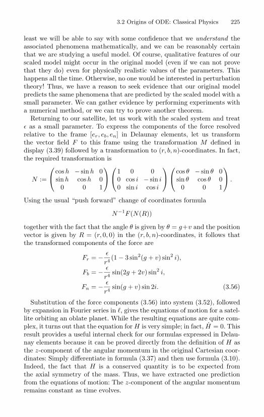
3.2 Origins of ODE: Classical Physics 225
least we will be able to say with some confidence that we understand theassociated phenomena mathematically, and we can be reasonably certainthat we are studying a useful model. Of course, qualitative features of ourscaled model might occur in the original model (even if we can not provethat they do) even for physically realistic values of the parameters. Thishappens all the time. Otherwise, no one would be interested in perturbationtheory! Thus, we have a reason to seek evidence that our original modelpredicts the same phenomena that are predicted by the scaled model with asmall parameter. We can gather evidence by performing experiments witha numerical method, or we can try to prove another theorem.
Returning to our satellite, let us work with the scaled system and treatε as a small parameter. To express the components of the force resolvedrelative to the frame [er, eb, en] in Delaunay elements, let us transformthe vector field F to this frame using the transformation M defined indisplay (3.39) followed by a transformation to (r, b, n)-coordinates. In fact,the required transformation is
N :=
cos h − sin h 0sin h cos h 0
0 0 1
1 0 00 cos i − sin i0 sin i cos i
cos θ − sin θ 0sin θ cos θ 0
0 0 1
.
Using the usual “push forward” change of coordinates formula
N−1F (N(R))
together with the fact that the angle θ is given by θ = g+v and the positionvector is given by R = (r, 0, 0) in the (r, b, n)-coordinates, it follows thatthe transformed components of the force are
Fr = − ε
r4 (1 − 3 sin2(g + v) sin2 i),
Fb = − ε
r4 sin(2g + 2v) sin2 i,
Fn = − ε
r4 sin(g + v) sin 2i. (3.56)
Substitution of the force components (3.56) into system (3.52), followedby expansion in Fourier series in , gives the equations of motion for a satel-lite orbiting an oblate planet. While the resulting equations are quite com-plex, it turns out that the equation for H is very simple; in fact, H = 0. Thisresult provides a useful internal check for our formulas expressed in Delau-nay elements because it can be proved directly from the definition of H asthe z-component of the angular momentum in the original Cartesian coor-dinates: Simply differentiate in formula (3.37) and then use formula (3.10).Indeed, the fact that H is a conserved quantity is to be expected fromthe axial symmetry of the mass. Thus, we have extracted one predictionfrom the equations of motion: The z-component of the angular momentumremains constant as time evolves.
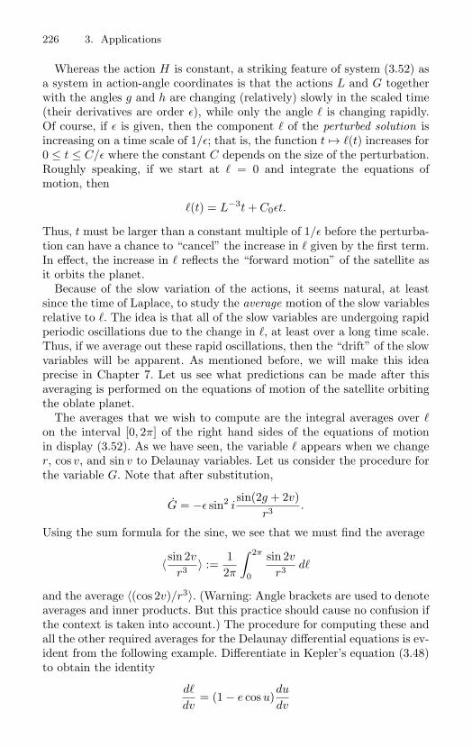
226 3. Applications
Whereas the action H is constant, a striking feature of system (3.52) asa system in action-angle coordinates is that the actions L and G togetherwith the angles g and h are changing (relatively) slowly in the scaled time(their derivatives are order ε), while only the angle is changing rapidly.Of course, if ε is given, then the component of the perturbed solution isincreasing on a time scale of 1/ε; that is, the function t → (t) increases for0 ≤ t ≤ C/ε where the constant C depends on the size of the perturbation.Roughly speaking, if we start at = 0 and integrate the equations ofmotion, then
(t) = L−3t + C0εt.
Thus, t must be larger than a constant multiple of 1/ε before the perturba-tion can have a chance to “cancel” the increase in given by the first term.In effect, the increase in reflects the “forward motion” of the satellite asit orbits the planet.
Because of the slow variation of the actions, it seems natural, at leastsince the time of Laplace, to study the average motion of the slow variablesrelative to . The idea is that all of the slow variables are undergoing rapidperiodic oscillations due to the change in , at least over a long time scale.Thus, if we average out these rapid oscillations, then the “drift” of the slowvariables will be apparent. As mentioned before, we will make this ideaprecise in Chapter 7. Let us see what predictions can be made after thisaveraging is performed on the equations of motion of the satellite orbitingthe oblate planet.
The averages that we wish to compute are the integral averages over on the interval [0, 2π] of the right hand sides of the equations of motionin display (3.52). As we have seen, the variable appears when we changer, cos v, and sin v to Delaunay variables. Let us consider the procedure forthe variable G. Note that after substitution,
G = −ε sin2 isin(2g + 2v)
r3 .
Using the sum formula for the sine, we see that we must find the average
〈 sin 2v
r3 〉 :=12π
∫ 2π
0
sin 2v
r3 d
and the average 〈(cos 2v)/r3〉. (Warning: Angle brackets are used to denoteaverages and inner products. But this practice should cause no confusion ifthe context is taken into account.) The procedure for computing these andall the other required averages for the Delaunay differential equations is ev-ident from the following example. Differentiate in Kepler’s equation (3.48)to obtain the identity
d
dv= (1 − e cos u)
du
dv
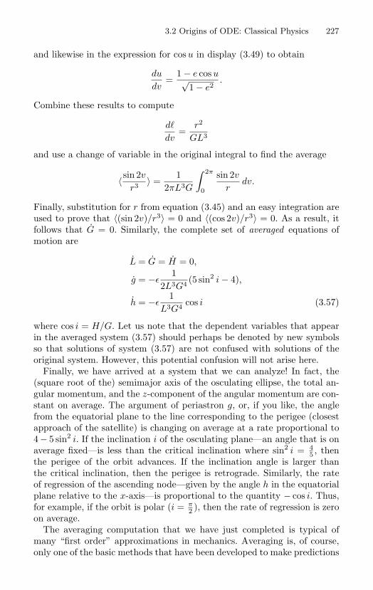
3.2 Origins of ODE: Classical Physics 227
and likewise in the expression for cos u in display (3.49) to obtain
du
dv=
1 − e cos u√1 − e2
.
Combine these results to compute
d
dv=
r2
GL3
and use a change of variable in the original integral to find the average
〈 sin 2v
r3 〉 =1
2πL3G
∫ 2π
0
sin 2v
rdv.
Finally, substitution for r from equation (3.45) and an easy integration areused to prove that 〈(sin 2v)/r3〉 = 0 and 〈(cos 2v)/r3〉 = 0. As a result, itfollows that G = 0. Similarly, the complete set of averaged equations ofmotion are
L = G = H = 0,
g = −ε1
2L3G4 (5 sin2 i − 4),
h = −ε1
L3G4 cos i (3.57)
where cos i = H/G. Let us note that the dependent variables that appearin the averaged system (3.57) should perhaps be denoted by new symbolsso that solutions of system (3.57) are not confused with solutions of theoriginal system. However, this potential confusion will not arise here.
Finally, we have arrived at a system that we can analyze! In fact, the(square root of the) semimajor axis of the osculating ellipse, the total an-gular momentum, and the z-component of the angular momentum are con-stant on average. The argument of periastron g, or, if you like, the anglefrom the equatorial plane to the line corresponding to the perigee (closestapproach of the satellite) is changing on average at a rate proportional to4 − 5 sin2 i. If the inclination i of the osculating plane—an angle that is onaverage fixed—is less than the critical inclination where sin2 i = 4
5 , thenthe perigee of the orbit advances. If the inclination angle is larger thanthe critical inclination, then the perigee is retrograde. Similarly, the rateof regression of the ascending node—given by the angle h in the equatorialplane relative to the x-axis—is proportional to the quantity − cos i. Thus,for example, if the orbit is polar (i = π
2 ), then the rate of regression is zeroon average.
The averaging computation that we have just completed is typical ofmany “first order” approximations in mechanics. Averaging is, of course,only one of the basic methods that have been developed to make predictions
228 3. Applications
from “realistic” systems of ordinary differential equations that originate incelestial mechanics.
Exercise 3.12. The fact that the perturbation force for the oblate planetcomes from a potential implies that the force is conservative. In fact, the per-turbed system in this case is Hamiltonian with the total energy, including thecorrection to the gravitational potential, as the Hamiltonian function. It turns outthat the coordinate change to Delaunay variables is of a very special type, calledcanonical. For a canonical change of coordinates it is not necessary to changevariables directly in the equations of motion. Instead, it suffices to change vari-ables in the Hamiltonian function and then to derive the new equations of motionin the usual way from the transformed Hamiltonian (see Section 1.7). Show, byconstructing an example, that a general change of coordinates is not canonical.Assume that the Delaunay coordinates are canonical, write the Hamiltonian inDelaunay variables, and derive from it the Hamiltonian equations of motion inDelaunay variables. In particular, show, using the form of the Hamiltonian differ-ential equations, that the average of L over the angle must vanish. This providesan internal check for the formulas derived in this section. Do you see how onemight obtain the averaged equations directly from the Hamiltonian? One reasonwhy the Hamiltonian approach was not used in the derivation of the equationsin Delaunay elements is that we have not developed the theory required to provethat the change to Delaunay variables is canonical. Another reason is that ourapproach works even if the perturbing force is not conservative.
3.2.5 The Diamagnetic Kepler ProblemIn this section we will derive equations of motion for the electron of thehydrogen atom in a magnetic field. The purpose of the section is to showthat some of the usual theory of Lagrangian and Hamiltonian mechanicsmay be viewed as a method to study a certain class of differential equations.In particular, we will use some ideas from classical mechanics to reduce theequations of motion to a form where Delaunay variables and the methodof averaging are applicable.
Consider the classical equations for the motion of an electron of an atomin the presence of a constant magnetic field. Let us assume that the electronis subjected to the Coulomb potential relative to the nucleus of the atomand to the Lorentz force due to the constant magnetic field B. If q is thecharge of an electron and Z is the atomic number of the atom, and if, asusual, R is the position of the electron relative to Cartesian coordinatescentered at the nucleus, V is the velocity of the electron, and r := |R|, thenthe Coulomb potential is
U :=kZq(−q)
r= −kZq2
r
where k is a constant. (Note the similarity to the gravitational potential!)In our choice of units, q is measured in coulombs and kq2, often denoted
3.2 Origins of ODE: Classical Physics 229
e2 in physics where of course e is not the eccentricity, has value kq2 ≈(1.52 × 10⁻¹⁴)2Nm2 in mks units where N is used to denote newtons. Forthe rest of this section let us suppose that Z = 1, the atomic number ofthe hydrogen atom.
Let us assume that the constant magnetic field B is parallel to the z-axisand that the electric field E vanishes. Then, as we have seen previously,the Lorentz force is given by
qV × B.
According to Newton’s law, the equations of motion are given in vectorform by
p = qV × B − kq2
r3 R (3.58)
where p is the momentum. Because the speed of the electron of a hydrogenatom is about one percent of the speed of light ([66]), let us use the classicalmomentum p = mV .
Equation (3.58) will be reduced to a somewhat simpler and more usefulform by a change of coordinates. From a mathematical point of view, thereduction is rather simple. However, the motivation for the reduction is theresult of at least half a century of physics.
Let us recast system (3.58) in the form
d
dt(p − 1
2q(R × B)) =
12q(V × B) − gradU. (3.59)
This first step may appear to arrive out of thin air. In fact, it is justthe bridge from Newtonian to Lagrangian mechanics. As we will see in amoment, system (3.59) is in the form of an Euler–Lagrange equation.
In physics, a new vector field A, called the vector potential, is introducedso that B = curlA. For our constant magnetic field, an easy computationshows that A = 1
2B × R. This vector field can be substituted into theleft hand side of equation (3.59) and used in the rest of the computation.However, let us continue using the original fields.
If we define the Lagrangian
L :=1
2m〈p, p〉 +
q
2〈B × R, V 〉 − U,
then, using a vector identity, we have
∂L∂V
= p − q
2〈R × B, V 〉,
∂L∂R
= −q
2∂
∂R〈R,B × V 〉 − gradU
=q
2V × B − gradU ;
230 3. Applications
that is, equation (3.59) with Q := R = (x, y, z) is exactly
d
dt
( ∂L∂Q
)=
∂L∂Q . (3.60)
In view of our derivation of the Euler–Lagrange equation in Section 3.1, wehave reason to expect that there is a variational principle associated withthe differential equation (3.60). This is indeed the case (see [104]).
The position variable Q and the velocity variable Q define a coordinatesystem on R
3 × R3. Let us define a new variable
P :=∂L∂Q
(Q, Q) = p − q
2Q × B (3.61)
and note that the relation (3.61) can be inverted to obtain Q as a functionof Q and P. In fact, there is a function α such that
P ≡ ∂L∂Q
(Q, α(Q,P)).
Thus, we have defined new coordinates (P,Q) on R3 × R
3.The reason for introducing P is so that we can define the Hamiltonian
H := PQ − L(Q, Q) = Pα(Q,P) − L(Q, α(Q,P)).
This terminology is justified by the following results:
∂H∂P = Q +
(P − ∂L
∂Q) ∂α
∂P = Q,
∂H∂Q = − ∂L
∂Q= − d
dt
∂L∂Q
= −P.
Thus, the original system is equivalent to the Hamiltonian system withHamiltonian H. In particular, H is constant along orbits.
By the definition of H, we have
H = 〈p +q
2(B × R), V 〉 − 1
2m〈p, p〉 − q
2〈B × R, V 〉 − U(Q)
=1
2m〈p, p〉 − U(Q)
=1
2m〈P +
q
2Q × B,P +
q
2Q × B〉 − U(Q).
If we take the constant magnetic field B := (0, 0, b), then
H =1
2m
(P2
1 + P22 + P2
3)
+ ω(yP1 − xP2) +mω2
2(x2 + y2) − kq2
r(3.62)
3.2 Origins of ODE: Classical Physics 231
where ω := 12mqb is called the Larmor frequency. Here, the magnitude b
of the magnetic field has units N sec/(coul m) and the Larmor frequency ωhas units 1/sec.
An essential result for the Hamiltonian system with Hamiltonian (3.62)is that the angular momentum function
(x, y, z,P1,P2,P3) → yP1 − xP2 (3.63)
is constant on orbits (see Exercise 3.13). Using this fact, if we consider onlyelectrons with zero angular momentum, then we may as well consider theequations of motion for the reduced Hamiltonian
H∗ =1
2m
(P2
1 + P22 + P2
3)
+mω2
2(x2 + y2) − kq2
r. (3.64)
Because of the analogy with the perturbed Kepler motion, this is calledthe diamagnetic Kepler problem ([82]). The corresponding Hamiltonianequations of motion are
x =1m
P1, y =1m
P2, z =1m
P3,
P1 = −(kq2
r3 x + mω2x),
P2 = −(kq2
r3 y + mω2y),
P3 = −kq2
r3 z. (3.65)
Equivalently, we have the second order system
mx = −kq2
r3 x − mω2x,
my = −kq2
r3 y − mω2y,
mz = −kq2
r3 z (3.66)
which is given in vector form by
R = −kq2m−1
r3 R + F0 (3.67)
where F0 = −ω2(x, y, 0). This last system is completely analogous to theequation for relative motion of the perturbed two-body problem.
What have we accomplished? We have used some ideas from classicalmechanics to find a reduction of the original equations of motion to a formwhere we can apply all of the analysis we have developed for the Kepler
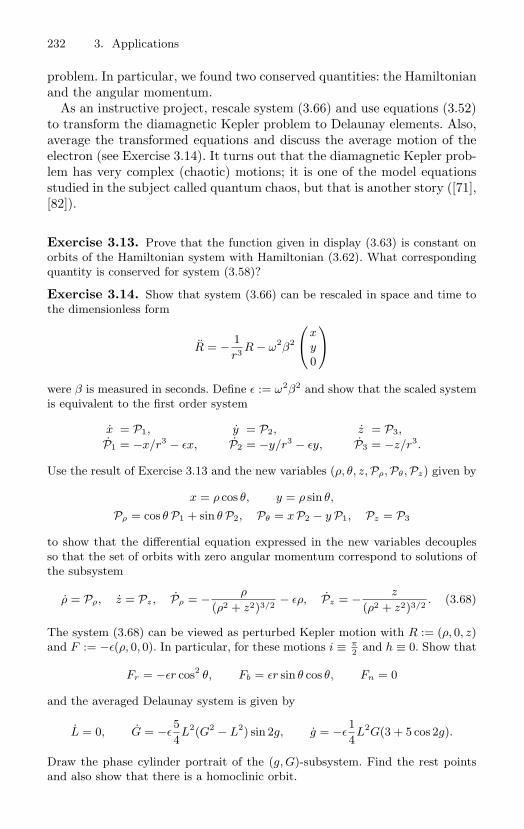
232 3. Applications
problem. In particular, we found two conserved quantities: the Hamiltonianand the angular momentum.
As an instructive project, rescale system (3.66) and use equations (3.52)to transform the diamagnetic Kepler problem to Delaunay elements. Also,average the transformed equations and discuss the average motion of theelectron (see Exercise 3.14). It turns out that the diamagnetic Kepler prob-lem has very complex (chaotic) motions; it is one of the model equationsstudied in the subject called quantum chaos, but that is another story ([71],[82]).
Exercise 3.13. Prove that the function given in display (3.63) is constant onorbits of the Hamiltonian system with Hamiltonian (3.62). What correspondingquantity is conserved for system (3.58)?
Exercise 3.14. Show that system (3.66) can be rescaled in space and time tothe dimensionless form
R = − 1r3 R − ω2β2
x
y0
were β is measured in seconds. Define ε := ω2β2 and show that the scaled systemis equivalent to the first order system
x = P1, y = P2, z = P3,
P1 = −x/r3 − εx, P2 = −y/r3 − εy, P3 = −z/r3.
Use the result of Exercise 3.13 and the new variables (ρ, θ, z, Pρ, Pθ, Pz) given by
x = ρ cos θ, y = ρ sin θ,
Pρ = cos θ P1 + sin θ P2, Pθ = x P2 − y P1, Pz = P3
to show that the differential equation expressed in the new variables decouplesso that the set of orbits with zero angular momentum correspond to solutions ofthe subsystem
ρ = Pρ, z = Pz, Pρ = − ρ
(ρ2 + z2)3/2 − ερ, Pz = − z
(ρ2 + z2)3/2 . (3.68)
The system (3.68) can be viewed as perturbed Kepler motion with R := (ρ, 0, z)and F := −ε(ρ, 0, 0). In particular, for these motions i ≡ π
2 and h ≡ 0. Show that
Fr = −εr cos2 θ, Fb = εr sin θ cos θ, Fn = 0
and the averaged Delaunay system is given by
L = 0, G = −ε54L2(G2 − L2) sin 2g, g = −ε
14L2G(3 + 5 cos 2g).
Draw the phase cylinder portrait of the (g, G)-subsystem. Find the rest pointsand also show that there is a homoclinic orbit.
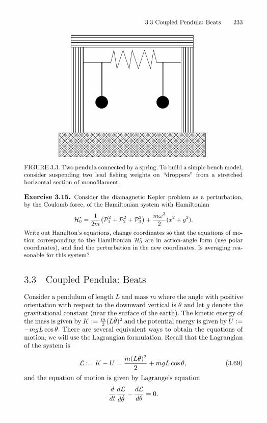
3.3 Coupled Pendula: Beats 233
FIGURE 3.3. Two pendula connected by a spring. To build a simple bench model,consider suspending two lead fishing weights on “droppers” from a stretchedhorizontal section of monofilament.
Exercise 3.15. Consider the diamagnetic Kepler problem as a perturbation,by the Coulomb force, of the Hamiltonian system with Hamiltonian
H∗0 =
12m
(P21 + P2
2 + P23)
+mω2
2(x2 + y2).
Write out Hamilton’s equations, change coordinates so that the equations of mo-tion corresponding to the Hamiltonian H∗
0 are in action-angle form (use polarcoordinates), and find the perturbation in the new coordinates. Is averaging rea-sonable for this system?
3.3 Coupled Pendula: Beats
Consider a pendulum of length L and mass m where the angle with positiveorientation with respect to the downward vertical is θ and let g denote thegravitational constant (near the surface of the earth). The kinetic energy ofthe mass is given by K := m
2 (Lθ)2 and the potential energy is given by U :=−mgL cos θ. There are several equivalent ways to obtain the equations ofmotion; we will use the Lagrangian formulation. Recall that the Lagrangianof the system is
L := K − U =m(Lθ)2
2+ mgL cos θ, (3.69)
and the equation of motion is given by Lagrange’s equation
d
dt
dLdθ
− dLdθ
= 0.
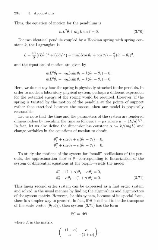
234 3. Applications
Thus, the equation of motion for the pendulum is
mL2θ + mgL sin θ = 0. (3.70)
For two identical pendula coupled by a Hookian spring with spring con-stant k, the Lagrangian is
L =m
2((Lθ1)2 + (Lθ2)2
)+ mgL(cos θ1 + cos θ2) − k
2(θ1 − θ2)2,
and the equations of motion are given by
mL2θ1 + mgL sin θ1 + k(θ1 − θ2) = 0,mL2θ2 + mgL sin θ2 − k(θ1 − θ2) = 0.
Here, we do not say how the spring is physically attached to the pendula. Inorder to model a laboratory physical system, perhaps a different expressionfor the potential energy of the spring would be required. However, if thespring is twisted by the motion of the pendula at the points of supportrather than stretched between the masses, then our model is physicallyreasonable.
Let us note that the time and the parameters of the system are rendereddimensionless by rescaling the time as follows: t = µs where µ := (L/g)1/2.In fact, let us also define the dimensionless constant α := k/(mgL) andchange variables in the equations of motion to obtain
θ′′1 + sin θ1 + α(θ1 − θ2) = 0,
θ′′2 + sin θ2 − α(θ1 − θ2) = 0.
To study the motions of the system for “small” oscillations of the pen-dula, the approximation sin θ ≈ θ—corresponding to linearization of thesystem of differential equations at the origin—yields the model
θ′′1 + (1 + α)θ1 − αθ2 = 0,
θ′′2 − αθ1 + (1 + α)θ2 = 0. (3.71)
This linear second order system can be expressed as a first order systemand solved in the usual manner by finding the eigenvalues and eigenvectorsof the system matrix. However, for this system, because of its special form,there is a simpler way to proceed. In fact, if Θ is defined to be the transposeof the state vector (θ1, θ2), then system (3.71) has the form
Θ′′ = AΘ
where A is the matrix (−(1 + α) α
α −(1 + α)
).

3.3 Coupled Pendula: Beats 235
The idea is to diagonalize the symmetric matrix A by a linear changeof variables of the form Z = BΘ where B is an orthogonal matrix. Incomponents, Z is the transpose of the vector (x, y) where
x =1√2(θ1 + θ2), y =
1√2(θ1 − θ2),
and the system in the new coordinates is given by
x′′ = −x, y′′ = −(1 + 2α)y.
There are two normal modes of oscillation. If y(s) ≡ 0, then θ1(s) −θ2(s) ≡ 0 and the pendula swing “in phase” with unit frequency relativeto the scaled time. If x(s) ≡ 0, then θ1(s) + θ2(s) ≡ 0 and the pendulaswing “in opposing phase” with frequency (1 + 2α)1/2 in the scaled time.The frequency of the second normal mode is larger than the frequency ofthe first normal mode due to the action of the spring; the spring has noeffect on the first normal mode.
Consider the following experiment. Displace the second pendulum by asmall amount and then release it from rest. What happens?
In our mathematical model, the initial conditions for the experiment are
θ1 = 0, θ′1 = 0, θ2 = a, θ′
2 = 0.
The corresponding motion of the system, with β :=√
1 + 2α, is given by
x(s) =a√2
cos s, y(s) = − a√2
cos βs,
and
θ1(s) =a
2(cos s − cos βs), θ2(s) =
a
2(cos s + cos βs).
Use the usual identities for cos(A ± B) with
A :=1 + β
2s, B :=
1 − β
2s,
to obtain
θ1(s) =(a sin
β − 12
s)sin
β + 12
s, θ2(s) =(a cos
β − 12
s)cos
β + 12
s,
and note that each pendulum swings with quasi-frequency 12 (β + 1) and
(relatively) slowly varying amplitude. Also, the “beats” of the two pendulaare out of phase. If s is approximately an integer multiple of 2π/(β − 1),then the first pendulum is almost motionless, Whereas if s is approximatelyan integer multiple of π/(β − 1), then the second pendulum is almost mo-tionless. This interesting exchange-of-energy phenomenon can be observedeven with very crude experimental apparatus—try it.
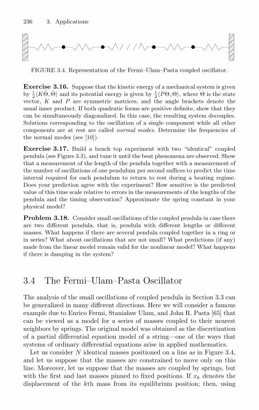
236 3. Applications
FIGURE 3.4. Representation of the Fermi–Ulam–Pasta coupled oscillator.
Exercise 3.16. Suppose that the kinetic energy of a mechanical system is givenby 1
2 〈KΘ, Θ〉 and its potential energy is given by 12 〈PΘ, Θ〉, where Θ is the state
vector, K and P are symmetric matrices, and the angle brackets denote theusual inner product. If both quadratic forms are positive definite, show that theycan be simultaneously diagonalized. In this case, the resulting system decouples.Solutions corresponding to the oscillation of a single component while all othercomponents are at rest are called normal modes. Determine the frequencies ofthe normal modes (see [10]).
Exercise 3.17. Build a bench top experiment with two “identical” coupledpendula (see Figure 3.3), and tune it until the beat phenomena are observed. Showthat a measurement of the length of the pendula together with a measurement ofthe number of oscillations of one pendulum per second suffices to predict the timeinterval required for each pendulum to return to rest during a beating regime.Does your prediction agree with the experiment? How sensitive is the predictedvalue of this time scale relative to errors in the measurements of the lengths of thependula and the timing observation? Approximate the spring constant in yourphysical model?
Problem 3.18. Consider small oscillations of the coupled pendula in case thereare two different pendula, that is, pendula with different lengths or differentmasses. What happens if there are several pendula coupled together in a ring orin series? What about oscillations that are not small? What predictions (if any)made from the linear model remain valid for the nonlinear model? What happensif there is damping in the system?
3.4 The Fermi–Ulam–Pasta Oscillator
The analysis of the small oscillations of coupled pendula in Section 3.3 canbe generalized in many different directions. Here we will consider a famousexample due to Enrico Fermi, Stanialaw Ulam, and John R. Pasta [65] thatcan be viewed as a model for a series of masses coupled to their nearestneighbors by springs. The original model was obtained as the discretizationof a partial differential equation model of a string—one of the ways thatsystems of ordinary differential equations arise in applied mathematics.
Let us consider N identical masses positioned on a line as in Figure 3.4,and let us suppose that the masses are constrained to move only on thisline. Moreover, let us suppose that the masses are coupled by springs, butwith the first and last masses pinned to fixed positions. If xk denotes thedisplacement of the kth mass from its equilibrium position; then, using
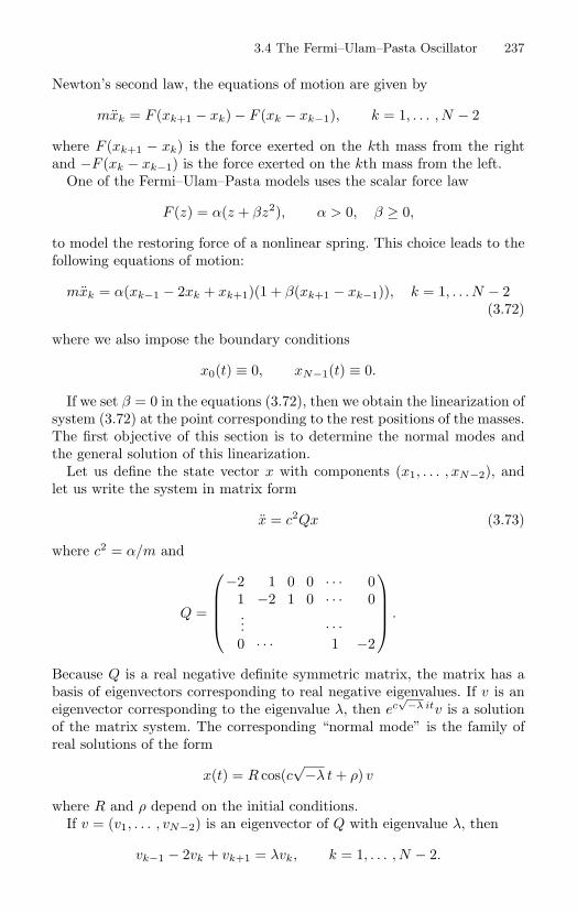
3.4 The Fermi–Ulam–Pasta Oscillator 237
Newton’s second law, the equations of motion are given by
mxk = F (xk+1 − xk) − F (xk − xk−1), k = 1, . . . , N − 2
where F (xk+1 − xk) is the force exerted on the kth mass from the rightand −F (xk − xk−1) is the force exerted on the kth mass from the left.
One of the Fermi–Ulam–Pasta models uses the scalar force law
F (z) = α(z + βz2), α > 0, β ≥ 0,
to model the restoring force of a nonlinear spring. This choice leads to thefollowing equations of motion:
mxk = α(xk−1 − 2xk + xk+1)(1 + β(xk+1 − xk−1)), k = 1, . . . N − 2(3.72)
where we also impose the boundary conditions
x0(t) ≡ 0, xN−1(t) ≡ 0.
If we set β = 0 in the equations (3.72), then we obtain the linearization ofsystem (3.72) at the point corresponding to the rest positions of the masses.The first objective of this section is to determine the normal modes andthe general solution of this linearization.
Let us define the state vector x with components (x1, . . . , xN−2), andlet us write the system in matrix form
x = c2Qx (3.73)
where c2 = α/m and
Q =
−2 1 0 0 · · · 0
1 −2 1 0 · · · 0... · · ·0 · · · 1 −2
.
Because Q is a real negative definite symmetric matrix, the matrix has abasis of eigenvectors corresponding to real negative eigenvalues. If v is aneigenvector corresponding to the eigenvalue λ, then ec
√−λ itv is a solutionof the matrix system. The corresponding “normal mode” is the family ofreal solutions of the form
x(t) = R cos(c√
−λ t + ρ) v
where R and ρ depend on the initial conditions.If v = (v1, . . . , vN−2) is an eigenvector of Q with eigenvalue λ, then
vk−1 − 2vk + vk+1 = λvk, k = 1, . . . , N − 2.
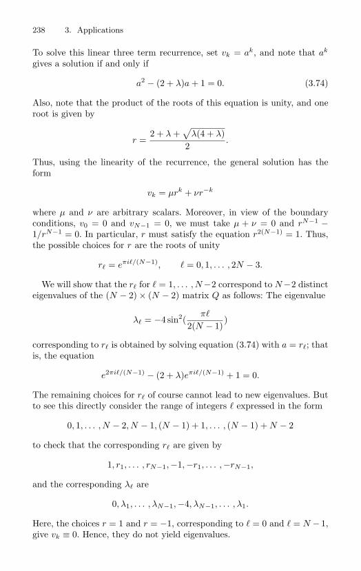
238 3. Applications
To solve this linear three term recurrence, set vk = ak, and note that ak
gives a solution if and only if
a2 − (2 + λ)a + 1 = 0. (3.74)
Also, note that the product of the roots of this equation is unity, and oneroot is given by
r =2 + λ +
√λ(4 + λ)
2.
Thus, using the linearity of the recurrence, the general solution has theform
vk = µrk + νr−k
where µ and ν are arbitrary scalars. Moreover, in view of the boundaryconditions, v0 = 0 and vN−1 = 0, we must take µ + ν = 0 and rN−1 −1/rN−1 = 0. In particular, r must satisfy the equation r2(N−1) = 1. Thus,the possible choices for r are the roots of unity
r = eπi/(N−1), = 0, 1, . . . , 2N − 3.
We will show that the r for = 1, . . . , N −2 correspond to N −2 distincteigenvalues of the (N − 2) × (N − 2) matrix Q as follows: The eigenvalue
λ = −4 sin2(π
2(N − 1))
corresponding to r is obtained by solving equation (3.74) with a = r; thatis, the equation
e2πi/(N−1) − (2 + λ)eπi/(N−1) + 1 = 0.
The remaining choices for r of course cannot lead to new eigenvalues. Butto see this directly consider the range of integers expressed in the form
0, 1, . . . , N − 2, N − 1, (N − 1) + 1, . . . , (N − 1) + N − 2
to check that the corresponding r are given by
1, r1, . . . , rN−1,−1,−r1, . . . ,−rN−1,
and the corresponding λ are
0, λ1, . . . , λN−1,−4, λN−1, . . . , λ1.
Here, the choices r = 1 and r = −1, corresponding to = 0 and = N − 1,give vk ≡ 0. Hence, they do not yield eigenvalues.
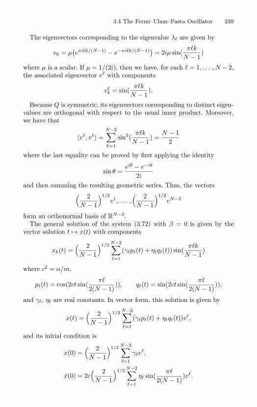
3.4 The Fermi–Ulam–Pasta Oscillator 239
The eigenvectors corresponding to the eigenvalue λ are given by
vk = µ(eπik/(N−1) − e−πik/(N−1)) = 2iµ sin(
πk
N − 1)
where µ is a scalar. If µ = 1/(2i), then we have, for each = 1, . . . , N − 2,the associated eigenvector v with components
vk = sin(
πk
N − 1).
Because Q is symmetric, its eigenvectors corresponding to distinct eigen-values are orthogonal with respect to the usual inner product. Moreover,we have that
〈v, v〉 =N−2∑k=1
sin2(πk
N − 1) =
N − 12
where the last equality can be proved by first applying the identity
sin θ =eiθ − e−iθ
2i
and then summing the resulting geometric series. Thus, the vectors( 2N − 1
)1/2v1, . . . ,
( 2N − 1
)1/2vN−2
form an orthonormal basis of RN−2.
The general solution of the system (3.72) with β = 0 is given by thevector solution t → x(t) with components
xk(t) =( 2
N − 1
)1/2 N−2∑=1
(γp(t) + ηq(t)) sin(πk
N − 1)
where c2 = α/m,
p(t) = cos(2ct sin(π
2(N − 1))), q(t) = sin(2ct sin(
π
2(N − 1))),
and γ, η are real constants. In vector form, this solution is given by
x(t) =( 2
N − 1
)1/2 N−2∑=1
(γp(t) + ηq(t))v,
and its initial condition is
x(0) =( 2
N − 1
)1/2 N−2∑=1
γv,
x(0) = 2c( 2
N − 1
)1/2 N−2∑=1
η sin(π
2(N − 1))v.
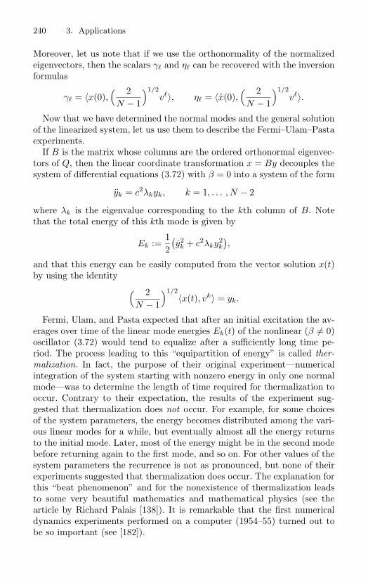
240 3. Applications
Moreover, let us note that if we use the orthonormality of the normalizedeigenvectors, then the scalars γ and η can be recovered with the inversionformulas
γ = 〈x(0),( 2
N − 1
)1/2v〉, η = 〈x(0),
( 2N − 1
)1/2v〉.
Now that we have determined the normal modes and the general solutionof the linearized system, let us use them to describe the Fermi–Ulam–Pastaexperiments.
If B is the matrix whose columns are the ordered orthonormal eigenvec-tors of Q, then the linear coordinate transformation x = By decouples thesystem of differential equations (3.72) with β = 0 into a system of the form
yk = c2λkyk, k = 1, . . . , N − 2
where λk is the eigenvalue corresponding to the kth column of B. Notethat the total energy of this kth mode is given by
Ek :=12(y2
k + c2λky2k
),
and that this energy can be easily computed from the vector solution x(t)by using the identity ( 2
N − 1
)1/2〈x(t), vk〉 = yk.
Fermi, Ulam, and Pasta expected that after an initial excitation the av-erages over time of the linear mode energies Ek(t) of the nonlinear (β = 0)oscillator (3.72) would tend to equalize after a sufficiently long time pe-riod. The process leading to this “equipartition of energy” is called ther-malization. In fact, the purpose of their original experiment—numericalintegration of the system starting with nonzero energy in only one normalmode—was to determine the length of time required for thermalization tooccur. Contrary to their expectation, the results of the experiment sug-gested that thermalization does not occur. For example, for some choicesof the system parameters, the energy becomes distributed among the vari-ous linear modes for a while, but eventually almost all the energy returnsto the initial mode. Later, most of the energy might be in the second modebefore returning again to the first mode, and so on. For other values of thesystem parameters the recurrence is not as pronounced, but none of theirexperiments suggested that thermalization does occur. The explanation forthis “beat phenomenon” and for the nonexistence of thermalization leadsto some very beautiful mathematics and mathematical physics (see thearticle by Richard Palais [138]). It is remarkable that the first numericaldynamics experiments performed on a computer (1954–55) turned out tobe so important (see [182]).
3.5 The Inverted Pendulum 241
Exercise 3.19. Solve the differential equation (3.73) by converting it to a firstorder system and then finding a basis of eigenvectors.
Exercise 3.20. Describe the geometry of the modes of oscillation of the massesin the Fermi–Ulam–Pasta model with respect to the linearized model (3.73). Forexample, is it possible that all the masses move so that the distances betweenadjacent masses stays fixed?
Exercise 3.21. Repeat the Fermi–Ulam–Pasta experiment. Begin with the pa-rameters
N = 32, m = 1.0, α = 1.0, β = 0.25,
and choose an initial condition so that the velocity of each mass is zero and allthe energy is in the first mode; for example, take
xk(0) =( 2
N − 1
)1/2sin(
πk
N − 1).
Integrate the system numerically and output the mode energies for at least thefirst few modes. Discuss how the mode energies change over time.
3.5 The Inverted Pendulum
Consider a pendulum with oscillating vertical displacement. We will outlinea proof of the following amazing fact: The inverted pendulum can be madestable for certain rapid oscillations of small vertical displacement. Historicalcomments on this observation together with a very interesting discussionof the phenomenon based on topological methods is given by Mark Levi(see [108]).
The equation of motion for the displaced inverted pendulum is obtainedas a modification of the pendulum model (3.70). For this, let H be a smooth(L/g)1/2-periodic function with unit amplitude where L is the length ofthe pendulum and g is the gravitational constant (the strange period ischosen for mathematical convenience). Also, let us incorporate two controlparameters, the amplitude δ and the (relative) frequency Ω of the verticaldisplacement, so that the displacement function is given by
t → δH(Ωt).
Then, the displacement may be viewed as an external force with period(L/g)1/2/Ω by taking the force to be
F := mLΩ2δH ′′(Ωt) sin θ.
An alternative way to view the model is to imagine the pendulum in an“Einstein elevator” that is being periodically accelerated. Then, the exter-nal force is perceived as a time-dependent change in the gravitational field.
242 3. Applications
In this case, the new gravitational “constant” measured in some units, saycm/sec/sec, is given by
g − Ω2δH ′′(Ωt),
and the equation of motion can be obtained by replacing g by this differencein the model (3.70). The minus sign is not important, it is there to make thisformulation compatible with the Lagrangian formulation. Indeed, with thechoice for the force given above and the Lagrangian (3.69), the Lagrangeequation
d
dt
dLdθ
− dLdθ
= F
yields the following equation of motion:
θ +g
Lsin θ = δ
Ω2
LH ′′(Ωt) sin θ.
As in Section 3.3, let us rescale time with the change of variable givenby
t =( L
Ω2g
)1/2s.
Also, after this change of time, let us use the scaled period and amplitudeof the displacement
α :=1
Ω2 , β := δ,
and the function given by
a(s) :=1gH ′′((L
g
)1/2s)
to construct the dimensionless equation of motion
θ′′ + (α − βa(s)) sin θ = 0 (3.75)
where the function s → a(s) is periodic with period one.To study the stability of the rest point at θ = π corresponding to the
inverted pendulum, let us linearize the equation of motion at θ = π toobtain the periodic linear system
w′′ − (α − βa(s))w = 0 (3.76)
with two dimensionless parameters, α and β. While we will consider the sys-tems corresponding to points (α, β) in the corresponding parameter plane,we must also keep in mind that only the points in the first quadrant of theparameter plane correspond to the physical parameters.
We will outline a proof of the following proposition:
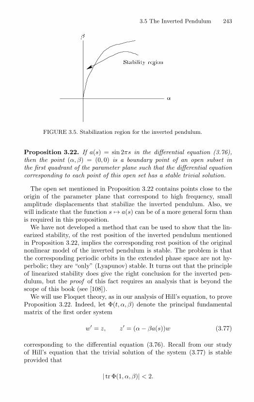
3.5 The Inverted Pendulum 243
Stability region
FIGURE 3.5. Stabilization region for the inverted pendulum.
Proposition 3.22. If a(s) = sin 2πs in the differential equation (3.76),then the point (α, β) = (0, 0) is a boundary point of an open subset inthe first quadrant of the parameter plane such that the differential equationcorresponding to each point of this open set has a stable trivial solution.
The open set mentioned in Proposition 3.22 contains points close to theorigin of the parameter plane that correspond to high frequency, smallamplitude displacements that stabilize the inverted pendulum. Also, wewill indicate that the function s → a(s) can be of a more general form thanis required in this proposition.
We have not developed a method that can be used to show that the lin-earized stability, of the rest position of the inverted pendulum mentionedin Proposition 3.22, implies the corresponding rest position of the originalnonlinear model of the inverted pendulum is stable. The problem is thatthe corresponding periodic orbits in the extended phase space are not hy-perbolic; they are “only” (Lyapunov) stable. It turns out that the principleof linearized stability does give the right conclusion for the inverted pen-dulum, but the proof of this fact requires an analysis that is beyond thescope of this book (see [108]).
We will use Floquet theory, as in our analysis of Hill’s equation, to proveProposition 3.22. Indeed, let Φ(t, α, β) denote the principal fundamentalmatrix of the first order system
w′ = z, z′ = (α − βa(s))w (3.77)
corresponding to the differential equation (3.76). Recall from our studyof Hill’s equation that the trivial solution of the system (3.77) is stableprovided that
| tr Φ(1, α, β)| < 2.
244 3. Applications
If (α, β) = (0, 0), then
Φ(1, 0, 0) = exp(
0 10 0
)=
(1 10 1
).
At this point of the parameter space tr Φ(1, 0, 0) = 2. Thus, it is reasonableto look for nearby points where tr Φ(1, 0, 0) < 2. The idea is simple enough:Under our assumption that H is smooth, so is the function τ : R
2 → R
given by (α, β) → tr Φ(1, α, β). We will use the implicit function theoremto show that the boundary of the region of stability is a smooth curvethat passes through the origin of the parameter space into the positive firstquadrant as depicted in Figure 3.5.
Let us compute the partial derivative τα(0, 0). For this, let A(s) denotethe system matrix for the system (3.77) and use the fact that Φ′ = A(s)Φto obtain the variational initial value problem
Φ′α = A(s)Φα + Aα(s)Φ, Φ′
α(0) = 0.
At (α, β) = (0, 0), the variational equation is given by the following linearsystem
W ′ =(
0 10 0
)W +
(0 01 0
)Φ(s, 0, 0)
=(
0 10 0
)W +
(0 01 0
)(1 s0 1
)=
(0 10 0
)W +
(0 01 s
)which can be solved by variation of parameters to obtain
Φα(1, 0, 0) = W (1) =( 1
2 ∗∗ 1
2
).
Therefore, we have that τα(0, 0) = 1.Define the function g(α, β) := τ(α, β) − 2 and note that we now have
g(0, 0) = 0, gα(0, 0) = 1.
By an application of the implicit function theorem, there is a function β →γ(β), defined for sufficiently small β, such that γ(0) = 0 and τ(γ(β), β) ≡ 2.
To determine which “side” of the curve Γ, defined by β → (β, γ(β)),corresponds to the region of stability, let us consider points on the positiveα-axis. In this case, the linearized equation has constant coefficients:
w′′ − αw = 0.
The principal fundamental matrix solution after “time” s = 1 is given by(cosh
√α 1√
αsinh
√α√
α sinh√
α cosh√
α
),
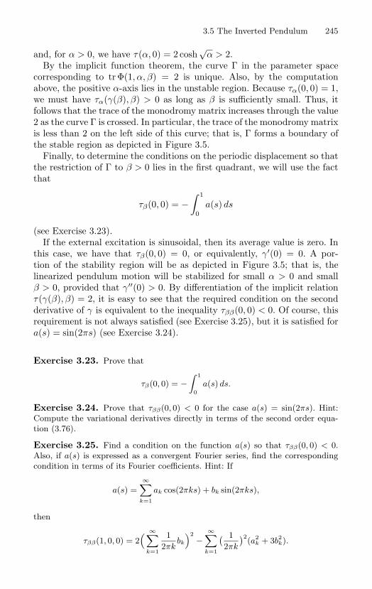
3.5 The Inverted Pendulum 245
and, for α > 0, we have τ(α, 0) = 2 cosh√
α > 2.By the implicit function theorem, the curve Γ in the parameter space
corresponding to tr Φ(1, α, β) = 2 is unique. Also, by the computationabove, the positive α-axis lies in the unstable region. Because τα(0, 0) = 1,we must have τα(γ(β), β) > 0 as long as β is sufficiently small. Thus, itfollows that the trace of the monodromy matrix increases through the value2 as the curve Γ is crossed. In particular, the trace of the monodromy matrixis less than 2 on the left side of this curve; that is, Γ forms a boundary ofthe stable region as depicted in Figure 3.5.
Finally, to determine the conditions on the periodic displacement so thatthe restriction of Γ to β > 0 lies in the first quadrant, we will use the factthat
τβ(0, 0) = −∫ 1
0a(s) ds
(see Exercise 3.23).If the external excitation is sinusoidal, then its average value is zero. In
this case, we have that τβ(0, 0) = 0, or equivalently, γ′(0) = 0. A por-tion of the stability region will be as depicted in Figure 3.5; that is, thelinearized pendulum motion will be stabilized for small α > 0 and smallβ > 0, provided that γ′′(0) > 0. By differentiation of the implicit relationτ(γ(β), β) = 2, it is easy to see that the required condition on the secondderivative of γ is equivalent to the inequality τββ(0, 0) < 0. Of course, thisrequirement is not always satisfied (see Exercise 3.25), but it is satisfied fora(s) = sin(2πs) (see Exercise 3.24).
Exercise 3.23. Prove that
τβ(0, 0) = −∫ 1
0a(s) ds.
Exercise 3.24. Prove that τββ(0, 0) < 0 for the case a(s) = sin(2πs). Hint:Compute the variational derivatives directly in terms of the second order equa-tion (3.76).
Exercise 3.25. Find a condition on the function a(s) so that τββ(0, 0) < 0.Also, if a(s) is expressed as a convergent Fourier series, find the correspondingcondition in terms of its Fourier coefficients. Hint: If
a(s) =∞∑
k=1
ak cos(2πks) + bk sin(2πks),
then
τββ(1, 0, 0) = 2( ∞∑
k=1
12πk
bk
)2−
∞∑k=1
( 12πk
)2(a2k + 3b2
k).
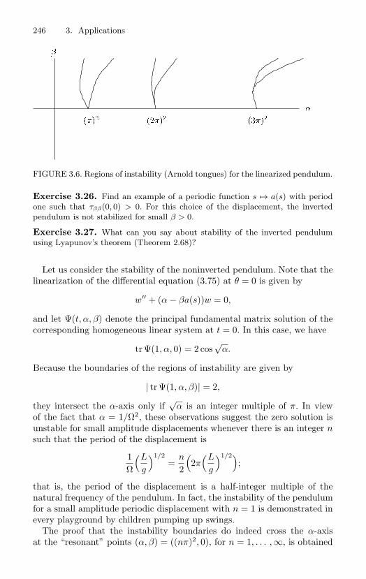
246 3. Applications
FIGURE 3.6. Regions of instability (Arnold tongues) for the linearized pendulum.
Exercise 3.26. Find an example of a periodic function s → a(s) with periodone such that τββ(0, 0) > 0. For this choice of the displacement, the invertedpendulum is not stabilized for small β > 0.
Exercise 3.27. What can you say about stability of the inverted pendulumusing Lyapunov’s theorem (Theorem 2.68)?
Let us consider the stability of the noninverted pendulum. Note that thelinearization of the differential equation (3.75) at θ = 0 is given by
w′′ + (α − βa(s))w = 0,
and let Ψ(t, α, β) denote the principal fundamental matrix solution of thecorresponding homogeneous linear system at t = 0. In this case, we have
tr Ψ(1, α, 0) = 2 cos√
α.
Because the boundaries of the regions of instability are given by
| tr Ψ(1, α, β)| = 2,
they intersect the α-axis only if√
α is an integer multiple of π. In viewof the fact that α = 1/Ω2, these observations suggest the zero solution isunstable for small amplitude displacements whenever there is an integer nsuch that the period of the displacement is
1Ω
(L
g
)1/2=
n
2
(2π
(L
g
)1/2);
that is, the period of the displacement is a half-integer multiple of thenatural frequency of the pendulum. In fact, the instability of the pendulumfor a small amplitude periodic displacement with n = 1 is demonstrated inevery playground by children pumping up swings.
The proof that the instability boundaries do indeed cross the α-axisat the “resonant” points (α, β) = ((nπ)2, 0), for n = 1, . . . ,∞, is obtained
3.6 Origins of ODE: Partial Differential Equations 247
from an analysis of the Taylor expansion of the function given by Ψ(1, α, β)at each resonant point (see Exercise 3.28). Typically, the instability regionsare as depicted in Figure 3.6. The instability region with n = 1 is “open”at β = 0 (the tangents to the boundary curves have distinct slopes); theremaining instability regions are “closed.” While it is an interesting math-ematical problem to determine the general shape of the stability regions([78], [115]), the model is, perhaps, not physically realistic for large β.
Exercise 3.28. Suppose that a(s) = sin(2πs) and set
g(α, β) = tr Ψ(1, α, β) − 2.
Show that gα((nπ)2, 0) = 0 and gβ((nπ)2, 0) = 0. Thus, the implicit functiontheorem cannot be applied directly to obtain the boundaries of the regions ofinstability, the boundary curves are singular at the points where they meet theα-axis. By computing appropriate higher order derivatives and analyzing theresulting Taylor expansion of g, show that the regions near the α-axis are indeedas depicted in Figure 3.6. Also, show that the regions become “thinner” as nincreases.
3.6 Origins of ODE: Partial Differential Equations
In this section there is an elementary discussion of three “big ideas”:
• Certain partial differential equations (PDE) can be viewed as ordi-nary differential equations with an infinite dimensional phase space.
• Finite dimensional approximations of some PDE are systems of ordi-nary differential equations.
• Traveling wave fronts in PDE can be described by ordinary differen-tial equations.
While these ideas are very important and therefore have been widely stud-ied, only a few elementary illustrations will be given here. The objectiveof this section is to introduce these ideas as examples of how ordinarydifferential equations arise and to suggest some very important areas forfurther study (see [27], [85], [84], [90], [135], [140], [162], [174], and [191]).We will also discuss the solution of first order PDE as an application of thetechniques of ordinary differential equations.
Most of the PDE mentioned in this section can be considered as mod-els of “reaction-diffusion” processes. To see how these models are derived,imagine some substance distributed in a medium. The density of the sub-stance is represented by a function u : R
n × R → R so that (x, t) → u(x, t)gives its density at the site with coordinate x at time t.
248 3. Applications
If Ω is a region in space with boundary ∂Ω, then the rate of change of theamount of the substance in Ω is given by the flux of the substance throughthe boundary of Ω plus the amount of the substance generated in Ω; thatis,
d
dt
∫Ω
u dV = −∫
∂ΩX · η dS +
∫Ω
f dV
where X is the vector field representing the motion of the substance; dVis the volume element; dS is the surface element; the vector field η is theouter unit normal field on the boundary of Ω; and f , a function of density,position and time, represents the amount of the substance generated in Ω.The minus sign on the flux term is required because we are measuring therate of change of the amount of substance in Ω. If, for example, the flowis all out of Ω, then X · η ≥ 0 and the minus sign is required because therate of change of the amount of substance in Ω must be negative.
If Stokes’ theorem is applied to rewrite the flux term and the time deriva-tive is interchanged with the integral of the density, then∫
Ωut dV = −
∫Ω
div X dV +∫
Ωf dV.
Moreover, by using the fact that the region Ω is arbitrary in the integralidentity, it is easy to prove the fundamental balance law
ut = − div X + f. (3.78)
To obtain a useful dynamical equation for u from equation (3.78), weneed a constitutive relation between the density u of the substance andthe flow field X. It is not at all clear how to derive this relationship fromthe fundamental laws of physics. Thus, we have an excellent example ofan important problem where physical intuition must be used to propose aconstitutive law whose validity can only be tested by comparing the resultsof experiments with the predictions of the corresponding model. Problemsof this type lie at the heart of applied mathematics and physics.
For equation (3.78), the classic constitutive relation—called Darcy’s,Fick’s, or Fourier’s law depending on the physical context—is
X = −K gradu + µV (3.79)
where K ≥ 0 and µ are functions of density, position, and time; and Vdenotes the flow field for the medium in which our substance is moving.The minus sign on the gradient term represents the assumption that thesubstance diffuses from higher to lower concentrations.
By inserting the relation (3.79) into the balance law (3.78), we obtainthe dynamical equation
ut = div(K gradu) − div(µV ) + f.
3.6 Origins of ODE: Partial Differential Equations 249
Also, if we assume that the diffusion coefficient K is equal to k2 for someconstant k, the function µ is given by µ(u, x, t) = γu where γ is a constant,and V is an incompressible flow field (div V = 0); then we obtain the mostoften used reaction-diffusion-convection model equation
ut + γ gradu · V = k2∆u + f. (3.80)
In this equation, the gradient term is called the convection term, the Lapla-cian term is called the diffusion term, and f is the source term. Let us alsonote that if the diffusion coefficient is zero, the convection coefficient isgiven by γ = 1, the source function vanishes, and V is not necessarily in-compressible, then equation (3.80) reduces to the law of conservation ofmass, also called the continuity equation, given by
ut + div(uV ) = 0. (3.81)
Because equation (3.80) is derived from general physical principles, thisPDE can be used to model many different phenomena. As a result, thereis a vast scientific literature devoted to its study. We will not be able toprobe very deeply, but we will use equation (3.80) to illustrate a few aspectsof the analysis of these models where ordinary differential equations arisenaturally.
3.6.1 Infinite Dimensional ODEA simple special case of the reaction-diffusion-convection model (3.80) isthe linear diffusion equation (the heat equation) in one spatial dimension,namely, the PDE
ut = k2uxx (3.82)
where k2 is the diffusivity constant. This differential equation can be usedto model heat flow in an insulated bar. In fact, let us suppose that the bar isidealized to be the interval [0, ] on the x-axis so that u(x, t) represents thetemperature of the bar at the point with coordinate x at time t. Moreover,because the bar has finite length, let us model the heat flow at the ends ofthe bar where we will consider just two possibilities: The bar is insulatedat both ends such that we have the Neumann boundary conditions
ux(0, t) = 0, ux(, t) = 0;
or, heat is allowed to flow through the ends of the bar, but the temperatureat the ends is held constant at zero (in some appropriate units) such thatwe have the Dirichlet boundary conditions
u(0, t) = 0, u(, t) = 0.
250 3. Applications
If one set of boundary conditions is imposed and an initial temperaturedistribution, say x → u0(x), is given on the bar, then we would expectthat there is a unique scalar function (x, t) → u(x, t), defined on the set[0, ] × [0,∞) that satisfies the PDE, the initial condition u(x, 0) = u0(x),and the boundary conditions. Of course, if such a solution exists, thenfor each t > 0, it predicts the corresponding temperature distributionx → u(x, t) on the bar. In addition, if there is a solution of the bound-ary value problem corresponding to each initial temperature distribution,then we have a situation that is just like the phase flow of an ordinary dif-ferential equation. Indeed, let us consider a linear space E of temperaturedistributions on the rod and let us suppose that if a function v : [0, ] → R
is in E , then there is a solution (x, t) → u(x, t) of the boundary value prob-lem with v as the initial temperature distribution such that x → u(x, t) isa function in E whenever t > 0. In particular, all the functions in E mustsatisfy the boundary conditions. If this is the case, then we have defined afunction (0,∞) × E → E given by (t, v) → ϕt(v) such that ϕ0(v)(x) = v(x)and (x, t) → ϕt(v)(x) is the solution of the boundary value problem withinitial temperature distribution v. In other words, we have defined a dy-namical system with “flow” ϕt whose phase space is the function spaceE of possible temperature distributions on the bar. For example, for theDirichlet problem, we might take E to be the subset of C2[0, ] consistingof those functions that vanish at the ends of the interval [0, ].
Taking our idea a step farther, let us define the linear transformation Aon E by
Au = k2uxx.
Then, the PDE (3.82) can be rewritten as
u = Au, (3.83)
an ordinary differential equation on the infinite dimensional space E . Also,to remind ourselves of the boundary conditions, let us write A = ANif Neumann boundary conditions are imposed and A = AD for Dirichletboundary conditions.
The linear homogeneous differential equation (3.83) is so simple thatits solutions can be given explicitly. However, we will see how the generalsolution of the PDE can be found by treating it as an ordinary differentialequation.
Let us begin by determining the rest points of the system (3.83). In fact, arest point is a function v : [0, ] → R that satisfies the boundary conditionsand the second order ordinary differential equation vxx = 0. Clearly, theonly possible choices are affine functions of the form v = cx+d where c andd are real numbers. There are two cases: For AN we must have c = 0, but dis a free variable. Thus, there is a line in the function space E correspondingto the constant functions in E that consists entirely of rest points. For the
3.6 Origins of ODE: Partial Differential Equations 251
Dirichlet case, both c and d must vanish and there is a unique rest pointat the origin of the phase space.
Having found the rest points for the differential equation (3.83), let usdiscuss their stability. By analogy with the finite dimensional case, let usrecall that we have discussed two methods that can be used to determinethe stability of rest points: linearization and Lyapunov’s direct method.In particular, for the finite dimensional case, the method of linearization isvalid as long as the rest point is hyperbolic, and, in this case, the eigenvaluesof the system matrix for the linearized system at the rest point determineits stability type.
Working formally, let us apply the method of linearization at the restpoints of the system (3.83). Since this differential equation is already linear,we might expect the stability of these rest points to be determined froman analysis of the position in the complex plane of the eigenvalues of thesystem operator A. By definition, if λ is an eigenvalue of the operator ADor AN , then there must be a nonzero function v on the interval [0, ] thatsatisfies the boundary conditions and the ordinary differential equation
k2vxx = λv.
If v is an eigenfunction with eigenvalue λ, then we have that∫
0k2vxxv dx =
∫
0λv2 dx. (3.84)
Let us suppose that v is square integrable, that is,∫
0v2 dx < ∞
and also smooth enough so that integration by parts is valid. Then, equa-tion (3.84) is equivalent to the equation
vxv∣∣∣0
−∫
0v2
x dx =λ
k2
∫
0v2 dx.
Thus, if either Dirichlet or Neumann boundary conditions are imposed,then the boundary term from the integration by parts vanishes, and there-fore the eigenvalue λ must be a nonpositive real number.
For AD, if λ = 0, then there is no nonzero eigenfunction. If λ < 0, thenthe eigenvalue equation has the general solution
v(x) = c1 cos αx + c2 sin αx
where α := (−λ)1/2/k and c1 and c2 are constants; and, in order to satisfythe Dirichlet boundary conditions, we must have(
1 0cos α sin α
)(c1c2
)=
(00
)
252 3. Applications
for some nonzero vector of constants. In fact, the determinant of the matrixmust vanish, and we therefore have to impose the condition that α is aninteger multiple of π; or equivalently,
λ = −(nπk
)2
with a corresponding eigenfunction given by
x → sinnπ
x
for each integer n = 1, 2, . . . ,∞. By a similar calculation for AN , we havethat λ = 0 is an eigenvalue with a corresponding eigenfunction v ≡ 1, andagain the same real numbers
λ = −(nπk
)2
are eigenvalues, but this time with corresponding eigenfunctions
x → cosnπ
x.
The nature of the real parts of the eigenvalues computed in the last para-graph and the principle of linearized stability suggest that the origin is anasymptotically stable rest point for the Dirichlet problem. On the otherhand, the rest points of the Neumann problem seem to be of a differenttype: each of these rest points would appear to have a one-dimensionalcenter manifold and an infinite dimensional stable manifold. All of thesestatements are true. But to prove them, certain modifications of the corre-sponding finite dimensional results are required. For example, the principleof linearized stability is valid for rest points of infinite dimensional ODEunder the assumption that all points in the spectrum of the operator givenby the linearized vector field at the rest point (in our case the operator A)have negative real parts that are bounded away from the imaginary axisin the complex plane (see, for example, [162, p. 114]). More precisely, therequired hypothesis is that there is some number α > 0 such that the realpart of every point in the spectrum of the operator is less than −α.
Recall that a complex number λ is in the spectrum of the linear operatorA if the operator A − λI does not have a bounded inverse. Of course, ifv = 0 is an eigenfunction with eigenvalue λ, then the operator A − λI isnot injective and indeed λ is in the spectrum. In a finite dimensional space,if an operator is injective, then it is invertible. Hence, the only complexnumbers in the spectrum of a finite dimensional linear operator are eigen-values. However, in an infinite dimensional space, there can be points inthe spectrum that are not eigenvalues (see [60]). For example, let us definethe space L2(0, ) to be all (real) functions v : [0, ] → R such that∫
0v2(x) dx < ∞ (3.85)
3.6 Origins of ODE: Partial Differential Equations 253
where we consider two such functions v and w to be equal if∫
0(v(x) − w(x))2 dx = 0,
and consider the operator B : L2 → L2 given by (Bf)(x) → xf(x). Thisoperator has no eigenvalues, yet the entire interval [0, ] is in its spectrum.(Why?)
The operators AD and AN , considered as operators defined in L2(0, ),have spectra that consist entirely of eigenvalues (pure point spectrum).However, to prove this claim we must first deal with the fact that theseoperators are not defined on all of L2. After all, a square integrable functiondoes not have to be differentiable. Instead, we can view our operators tobe defined on the subset of L2 consisting of those functions that have twoderivatives both contained in L2. Then, the claim about the spectra of ADand AN can be proved in two steps. First, if a complex number λ is not aneigenvalue, then for all w ∈ L2 there is some function v that satisfies theboundary conditions and the differential equation
k2vxx − λv = w.
In other words, there is an operator B : L2 → L2 given by Bw = v suchthat (A − λI)Bw = w. The fact that B is bounded is proved from theexplicit construction of B as an integral operator. Also, it can be provedthat B(A − λI)v = v for all v in the domain of A (see Exercise 3.29).Using these facts and the theorem on linearized stability mentioned above,it follows that the origin is an asymptotically stable rest point for theDirichlet problem.
Exercise 3.29. Show that the spectrum of the operator in L2(0, ) given byAv = vxx with either Dirichlet or Neumann boundary conditions consists only ofeigenvalues. Prove the same result for the operator Av = avxx + bvx + cv wherea, b, and c are real numbers.
In view of our results for finite dimensional linear systems, we expect thatif we have a linear evolution equation v = Av, even in an infinite dimen-sional phase space, and if Aw = λw, then etλw is a solution. This is indeedthe case for the PDE (3.82). Moreover, for linear evolution equations, wecan use the principle of superposition to deduce that every linear combi-nation of solutions of this type is again a solution. If we work formally,that is, without proving convergence, and if we use the eigenvalues andeigenvectors computed above, then the “general solution” of the Dirichletproblem is given by
u(x, t) =∞∑
n=1
e−( nπk )2tan sin
nπ
x,
254 3. Applications
and the general solution of the Neumann problem is given by
u(x, t) =∞∑
n=0
e−( nπk )2tbn cos
nπ
x
where an and bn are real numbers.If the initial condition u(x, 0) = u0(x) is given, then, for instance, for the
Dirichlet problem we must have that
u0(x) =∞∑
n=1
an sinnπ
x.
In other words, the initial function u0 must be represented by a Fouriersine series. What does this mean? The requirement is that the Fourier sineseries converges to u0 in the space L2 endowed with its natural norm,
‖v‖ :=(∫
0v2(x) dx
)1/2.
In fact, the inner product space L2 is a Hilbert space; that is, with respectto this norm, every Cauchy sequence in L2 converges (see [156]). The preciserequirement for u0 to be represented by a Fourier sine series is that thereare real numbers an and corresponding L2 partial sums
N∑n=1
an sinnπ
x
such that
limN→∞
‖u0 − uN‖ = 0.
If the initial function u0 is continuous, then for our special case the cor-responding solution obtained by Fourier series also converges pointwise toa C2 function that satisfies the PDE in the classical sense. We will show ina moment that this solution is unique, and therefore the special solutionsof the PDE obtained from the eigenvalues and corresponding eigenfunc-tions do indeed form a fundamental set of solutions for our boundary valueproblems.
There are several ways to prove that solutions of the diffusion equationwith a given initial condition are unique. We will use the “energy method”;an alternative uniqueness proof is based on the maximum principle (seeExercise 3.30). To show the uniqueness result, let us note that if two so-lutions of either the Dirichlet or Neumann boundary value problem satisfythe same initial condition, then the difference u of these two solutions is
3.6 Origins of ODE: Partial Differential Equations 255
a solution of the same boundary value problem but with initial value thezero function. Using an integration by parts, we also have the equality
d
dt
∫
0
12u2 dx =
∫
0utu dx = k2
∫
0uxxu dx = −k2
∫
0u2
x dx.
It follows that the function
t →∫
0
12u2(x, t) dx
is not increasing, and therefore it is bounded above by its value at t = 0,namely, ∫
0
12u2(x, 0) dx = 0.
The conclusion is that u(x, t) ≡ 0, as required.
Exercise 3.30. Prove the maximum principle: If ut(x, t) = k2uxx(x, t) is a C2
function on the open rectangle (0, ) × (0, T ) and a continuous function on theclosure of this rectangle, then the maximum of the function u is assumed eitheron the line (0, ) × 0 or on one of the lines
0 × [0, T ], × [0, T ].
Also, use the maximum principle to prove the uniqueness of solutions of theboundary value problem with initial condition for the diffusion equation. Hint:Use calculus (see [171, p. 41]).
Exercise 3.31. Solve the PDE (3.82) by the method of separation of variables;that is, assume that there is a solution of the form u(x, t) = p(x)q(t), substitutethis expression into the PDE, impose the boundary conditions, and determinethe general form of the functions p and q.
Using the explicit form of the Fourier series representations of the gen-eral solutions of the heat equation with Dirichlet or Neumann boundaryconditions, we can see that these solutions are very much like the solutionsof a homogeneous linear ordinary differential equation: They are expressedas superpositions of fundamental solutions and they obviously satisfy theflow property ϕs(ϕt(v)) = ϕs+t(v) as long as s and t are not negative (theseries solutions do not necessarily converge for t < 0). Because of this re-striction on the time variable, the solutions of our evolution equation aresaid to be semi-flows or semi-groups.
In the case of Dirichlet boundary conditions, if we look at the seriessolution, then we can see immediately that the origin is in fact globallyasymptotically stable. For the Neumann problem there is a one-dimensional
256 3. Applications
invariant manifold of rest points, and all other solutions are attracted expo-nentially fast to this manifold. Physically, if the temperature is held fixedat zero at the ends of the bar, then the temperature at each point of the barapproaches zero at an exponential rate, whereas if the bar is insulated atits ends, then the temperature at each point approaches the average valueof the initial temperature distribution.
Our discussion of the scalar diffusion equation, PDE (3.82), has servedto illustrate the fact that a (parabolic) PDE can be viewed as an ordinarydifferential equation on an infinite dimensional space. Moreover, as we haveseen, if we choose to study a PDE from this viewpoint, then our experiencewith ordinary differential equations can be used to advantage as a faithfulguide to its analysis.
Exercise 3.32. Verify the semi-flow property ϕs(ϕt(v)) = ϕs+t(v) for the solu-tions of the scalar heat equation with Dirichlet or Neumann boundary conditions.Generalize this result to the equation ut = uxx +f(u) under the assumption thatevery initial value problem for this equation has a local solution. Hint: How isthe flow property proved for finite dimensional autonomous equations?
Let us now consider the nonlinear PDE
ut = k2uxx + f(u, x, t), 0 < x < , t > 0 (3.86)
where f is a smooth function that represents a heat source in our heatconduction model.
To illustrate the analysis of rest points for a nonlinear PDE, let us as-sume that the source term f for the PDE (3.86) depends only on its firstvariable, and let us impose, as usual, either Dirichlet or Neumann boundaryconditions. In this situation, the rest points are given by those solutions ofthe ordinary differential equation
k2uxx + f(u) = 0 (3.87)
that also satisfy the Dirichlet or Neumann boundary conditions.The boundary value problem (3.87) is an interesting problem in ordinary
differential equations. Let us note first that if we view the independentvariable as “time,” then the second order differential equation (3.87) is justNewton’s equation for a particle of mass k2 moving in a potential forcefield with force −f(u). In addition, the corresponding first order system inthe phase plane is the Hamiltonian system
u = v, v = −f(u)
whose total energy is given by
H(u, v) :=k2
2v2 + F (u)
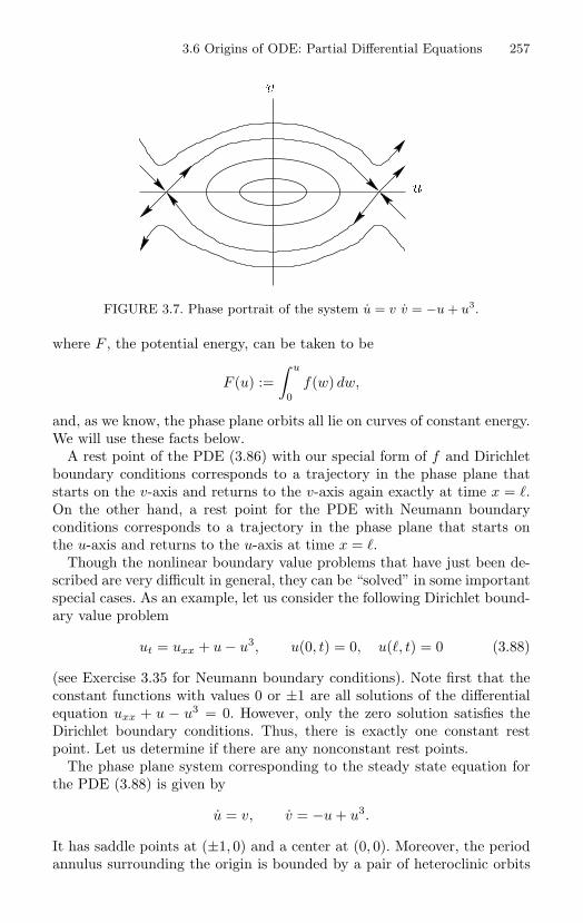
3.6 Origins of ODE: Partial Differential Equations 257
v
u
FIGURE 3.7. Phase portrait of the system u = v v = −u + u3.
where F , the potential energy, can be taken to be
F (u) :=∫ u
0f(w) dw,
and, as we know, the phase plane orbits all lie on curves of constant energy.We will use these facts below.
A rest point of the PDE (3.86) with our special form of f and Dirichletboundary conditions corresponds to a trajectory in the phase plane thatstarts on the v-axis and returns to the v-axis again exactly at time x = .On the other hand, a rest point for the PDE with Neumann boundaryconditions corresponds to a trajectory in the phase plane that starts onthe u-axis and returns to the u-axis at time x = .
Though the nonlinear boundary value problems that have just been de-scribed are very difficult in general, they can be “solved” in some importantspecial cases. As an example, let us consider the following Dirichlet bound-ary value problem
ut = uxx + u − u3, u(0, t) = 0, u(, t) = 0 (3.88)
(see Exercise 3.35 for Neumann boundary conditions). Note first that theconstant functions with values 0 or ±1 are all solutions of the differentialequation uxx + u − u3 = 0. However, only the zero solution satisfies theDirichlet boundary conditions. Thus, there is exactly one constant restpoint. Let us determine if there are any nonconstant rest points.
The phase plane system corresponding to the steady state equation forthe PDE (3.88) is given by
u = v, v = −u + u3.
It has saddle points at (±1, 0) and a center at (0, 0). Moreover, the periodannulus surrounding the origin is bounded by a pair of heteroclinic orbits
258 3. Applications
that lie on the curve
12v2 +
12u2 − 1
4u4 =
14
(see Figure 3.7). Using this fact, it is easy to see that the interval (0, 1/√
2)on the v-axis is a Poincare section for the annulus of periodic orbits. Also, aglance at the phase portrait of the system shows that only the solutions thatlie on these periodic orbits are candidates for nonconstant steady states forthe PDE; they are the only periodic orbits in the phase plane that meet thev-axis at more than one point. Also, let us notice that the phase portraitis symmetric with respect to each of the coordinate axes. In view of thissymmetry, if we define the period function
T :(0,
1√2
)→ R (3.89)
so that T (a) is the minimum period of the periodic solution starting atu(0) = 0, v(0) = a, then
u(12T (a)) = 0, v(
12T (a)) = −a.
Hence, solutions of our boundary value problem that correspond to restpoints for the PDE also correspond to periodic solutions whose half periodsare exactly some integer submultiple of ; equivalently, these solutions cor-respond to those real numbers a such that 0 < a < 1/
√2 and T (a) = 2/n
for some positive integer n. In fact, each such a corresponds to exactlytwo rest points of the PDE; namely, x → u(x) and x → u( − x) wherex → (u(x), v(x)) is the phase trajectory such that u(0) = 0 and v(0) = a.
The number and position in the phase plane of all rest point solutionsof the PDE can be determined from the following three propositions: (i)T (a) → 2π as a → 0+; (ii) T (a) → ∞ as a → (1/
√2)−; and (iii) T ′(a) > 0
(see Exercise 3.33). Using these facts, it follows that there is at most afinite number of rest points that correspond to the integers 1, 2, . . . , n suchthat n < /π.
Exercise 3.33. Prove that the period function T given in display (3.89) has apositive first derivative. One way to do this is to find the explicit time-dependentperiodic solutions of the first order system u = v, v = −u + u3 using ellipticfunctions. For a different method, see [29] and [153].
Exercise 3.34. Find the rest points for the Dirichlet boundary value problem
ut = uxx + au − bu2, u(x, 0) = 0, u(x, ) = 0
(see [35]).
3.6 Origins of ODE: Partial Differential Equations 259
Are the rest points of the PDE (3.88) stable? It turns out that the sta-bility problem for nonconstant rest points, even for our scalar PDE, is toodifficult to describe here (see [162, p. 530]). However, we can say some-thing about the stability of the constant rest point at the origin for thePDE (3.88). In fact, let us note that if < π, then it is the only rest point.Moreover, its stability can be determined by linearization.
Let us first describe the linearization procedure for a PDE. The correctformulation is simple if we view the PDE as an ordinary differential equa-tion on a function space. Indeed, we can just follow the recipe for linearizingan ordinary differential equation of the form u = g(u). Let us recall that ifz is a rest point and g is a smooth function, then the linearization of theordinary differential equation at z is
x = Dg(z)(x − z),
or equivalently
w = Dg(z)w
where w := x − z. Moreover, if the eigenvalues of Dg(z) all have negativereal parts, then the rest point z is asymptotically stable (see Section 2.3).
In order to linearize at a rest point of a PDE, let us suppose that thefunction x → z(x) is a rest point for the PDE
ut = g(u)
where g(u) := uxx + f(u) and f : R → R is a differentiable function. If thedomain of AD is viewed as the function space C2[0, ], then the functiong : C2[0, ] → C0[0, ] is differentiable. This follows because the functionu → uxx is linear and the function f is smooth. However, we have to becareful. In the definition of g we must view the notation f(u) to mean f uwhere u ∈ C2[0, ]. The difficulty is that the smoothness of the functionu → f u depends on the topology of the function space to which u belongs(see Example 1.153).
Once we know that g is differentiable, its derivative can be easily com-puted as a directional derivative; in fact,
Dg(z)v =d
dtg(z + tv)
∣∣∣t=0
= vxx + Df(z)v.
Therefore, by definition, the linearized equation at the rest point z is givenby
w = wxx + Df(z(x))w. (3.90)
For a nonconstant rest point, the linearized equation (3.90) depends onthe space variable x. The determination of stability in this case is often
260 3. Applications
quite difficult—-recall the stability analysis for periodic solutions of finitedimensional ordinary differential equations. For a constant rest point, thelinearized equation has the form w = Aw where A is the linear operatorgiven by w → wxx+Df(z)w for z a fixed number. In this case, as mentionedpreviously, it seems natural to expect the following result: If the spectrumof A is in the open left half plane and bounded away from the imaginaryaxis, then the rest point is asymptotically stable. In fact, this result, whenproperly interpreted, is true for the PDE (3.88). But to prove it, we haveto specify the function space on which the spectrum is to be computed andrecast the arguments used for ordinary differential equations in an infinitedimensional setting. For the PDE (3.88) the idea—derived from our studyof ordinary differential equations—of applying the principle of linearizedstability is justified, but some functional analysis is required to carry itout (see [162, Chapter 11]). However, our example is perhaps too simple;there are PDE where the linearized stability of a steady state can be easilyproved, but the stability of the rest point is an open question. The problemfor a general PDE of the form
ut = Au + f(u)
is that the linear operator A, the function f , and the linearized operatorA+Df(z) must all satisfy additional hypotheses before the ODE argumentsfor the validity of the principle of linearized stability can be verified in theinfinite dimensional case. This fact is an important difference between thetheory of ordinary differential equations and the theory of PDE.
Let us put aside the theoretical justification of linearized stability and re-consider the rest point at the origin for the PDE (3.88) where the linearizedsystem is given by
wt = wxx + w, w(0) = 0, w() = 0.
In this case, the spectrum of the differential operator defined by
Aw = wxx + w
consists only of eigenvalues (see Exercise 3.29). In fact, using the analysisof the spectrum of the operator w → wxx given above, the spectrum of Ais easily obtained by a translation. In fact, the spectrum is
1 −(nπ
)2: n = 1, 2, . . . ,∞
.
Because
1 −(nπ
)2≤ 1 −
(π
)2,
the spectrum of A lies in the left half of the complex plane and is boundedaway from the imaginary axis if and only if 1 < π2/2. Hence, using this
3.6 Origins of ODE: Partial Differential Equations 261
fact and assuming the validity of the principle of linearized stability, wehave the following proposition: If < π, then the origin is the only steadystate and it is asymptotically stable.
Let us go one step further in our qualitative analysis of the PDE ut =uxx + f(u) by showing that there are no periodic solutions. In fact, thisclaim is true independent of the choice of > 0 and for an arbitrary smoothsource function f . The idea for the proof, following the presentation in [162],is to show that there is a function (essentially a Lyapunov function) thatdecreases on orbits. In fact, let us define
E(u) = −∫
0
(12u(x)uxx(x) + F (u(x))
)dx
where F is an antiderivative of f and note that
E = −∫
0
(12utuxx +
12uutxx + f(u)ut
)dx.
After integration by parts twice for the integral of the second term inthe integrand, and after imposing either Dirichlet or Neumann boundaryconditions, it follows that
E = −∫
0(uxx + f(u))ut dx = −
∫
0(uxx + f(u))2 dx.
Hence, except for the rest points, the time derivative of E is negative alongorbits. In particular, there are no periodic orbits. Can the function E beused to give a proof of the stability of the rest point at the origin?
For the PDE (3.88) with < π we have now built up a rather completepicture of the phase portrait. In fact, we know enough to conjecture thatthere is a unique rest point that is globally asymptotically stable. Is thisconjecture true?
Exercise 3.35. Analyze the existence of rest points, the stability types of con-stant rest points, and the phase portrait for the Neumann boundary value prob-lem
ut = uxx + u − u3, ux(0, t) = 0, ux(, t) = 0.
Note that there are three constant rest points. Use equation (3.90) to determinetheir stability types.
3.6.2 Galerkin ApproximationSince most differential equations, ODE or PDE, cannot be “solved,” it isnatural to seek approximate solutions. Of course, numerical methods areused all the time to obtain approximate values of state variables. However,
262 3. Applications
in theory and practice the utility of approximation methods goes far beyondnumber crunching; for example, approximations are used to gain insightinto the qualitative behavior of dynamical systems, to test computer codes,and to obtain existence proofs. Indeed, approximation methods are centralelements of applied mathematics.
In this section we will take a brief look at a special case of Galerkin’smethod, one of the classic approximation methods for PDE. However, letus note that Galerkin’s method is just one of an array of methods thatare based on the idea of finding finite dimensional approximations of in-finite dimensional dynamical systems. Many other methods are based onthe idea of finding finite dimensional invariant (or approximately invariant)submanifolds in the infinite dimensional phase space. Of course, rest pointsand periodic orbits are finite dimensional invariant submanifolds. But theseare only the simplest examples. In fact, let us note that a rest point or aperiodic orbit might have an infinite dimensional stable manifold and afinite dimensional center manifold. In this case, the local dynamical behav-ior is determined by the dynamics on the center manifold because nearbyorbits are attracted to the center manifold. An important generalization ofthis basic situation is the concept of an inertial manifold. By definition, aninertial manifold M is a finite dimensional submanifold in the phase spacethat has two properties: M is positively invariant, and every solution isattracted to M at an exponential rate (see [174]).
In general, if there is an attracting finite dimensional invariant manifold,then the dynamical system restricted to this invariant set is an ordinarydifferential equation that models the asymptotic behavior of the full in-finite dimensional PDE. In particular, the ω-limit set of every solutionlies on this manifold. Thus, the existence of such an invariant manifoldprovides the theoretical basis for a complete understanding of the infinitedimensional dynamical system using the techniques of ordinary differentialequations. However, it is usually very difficult to prove the existence of at-tracting invariant manifolds. Moreover, even if an invariant manifold doesexist, it is often very difficult to obtain the detailed specification of thismanifold that would be required to reduce the original infinite dimensionaldynamical system to an ordinary differential equation. As an alternative,an approximation method—such as Galerkin’s method—that does not re-quire the existence of an invariant manifold can often be employed withgreat success.
The following philosophical question seems to accompany all theoreti-cal approximation methods for PDE “Is the set of reduced equations—presumably a system of nonlinear ordinary differential equations—easierto analyze than the original PDE?” In general, the answer to this ques-tion is clearly “no.” However, if the finite dimensional approximation is“low dimensional” or of some special form, then often qualitative analysisis possible, and useful insights into the dynamics of the original system canbe obtained. Perhaps the best “answer” to the question is to avoid the im-
3.6 Origins of ODE: Partial Differential Equations 263
plied choice between infinite dimensional and finite dimensional analysis.The best approach to an applied problem is with a mind free of prejudice.Often several different methods, including physical thinking and numericalanalysis, are required to obtain consistent and useful predictions from amodel.
Let us begin our discussion of the Galerkin approximation method withan elementary, but key idea. Recall that a (real) vector space H is an innerproduct space if there is a bilinear form (denoted here by angle brackets)such that if h ∈ H, then 〈h, h〉 ≥ 0 and 〈h, h〉 = 0 if and only if h = 0. Itfollows immediately that if v ∈ H and 〈v, h〉 = 0 for all h ∈ H, then v = 0.We will use this simple fact as the basis for solving equations in the spaceH. Indeed, suppose that we wish to find a solution of the (linear) equation
Au = b. (3.91)
If there is a vector u0 ∈ H such that 〈Au0 − b, h〉 = 0 for all h ∈ H, thenu0 is a solution of the equation.
If we identify a subspace S ⊂ H and find uS ∈ S such that
〈AuS − b, s〉 = 0
for all s ∈ S, then uS is called a Galerkin approximation of a solutionof equation (3.91). Of course, every h ∈ H is an “approximation” of asolution! The idea is to consider a sequence of subspaces, S1 ⊂ S2 ⊂ · · · that“converge” to H, and the corresponding Galerkin approximations un ∈ Sn
such that 〈Aun − b, s〉 = 0 for all s ∈ Sn. In this case, we might expect thatthe sequence u1, u2, . . . converges to a solution of the equation (3.91).
If H is a finite dimensional inner product space and the subspaces
S1, S2, S3, . . .
are strictly nested, then a corresponding sequence of Galerkin approxima-tions is finite. Thus, we do not have to worry about convergence. However,if H is an infinite dimensional Hilbert space, then the approximating sub-spaces must be chosen with care in order to ensure the convergence of thesequence of Galerkin approximations.
Let us recall that a sequence B = νi∞i=1 of linearly independent ele-
ments in H is called a Hilbert space basis if the linear manifold S spannedby B—all finite linear combinations of elements in B—is dense in H; thatis, if h ∈ H, then there is a sequence in S that converges to h in the naturalnorm defined from the inner product.
Suppose that H is a Hilbert space, B = νi∞i=1 is a Hilbert space basis
for H, and A : H → H is a linear operator. Also, for each positive integern let Sn denote the linear manifold spanned by the finite set ν1, . . . , νn.The Galerkin principle may be stated as follows: For each positive integern, there is some un ∈ Sn such that 〈Aun−b, s〉 = 0 for all s ∈ Sn. Moreover,the sequence un∞
n=1 converges to a solution of the equation Au = b.
264 3. Applications
The Galerkin principle is not a theorem! In fact, the Galerkin approxima-tions may not exist or the sequence of approximations may not converge.The applicability of the method depends on the equation we propose tosolve, the choice of the space H, and the choice of the basis B.
As an illustration of the Galerkin method applied to a PDE, let us con-sider the steady state equation
uxx + f(x) = 0, 0 < x < , (3.92)
with either Dirichlet or Neumann boundary conditions where f is a smoothfunction. We will formulate a variational (weak) form for this boundaryvalue problem. The basic idea is based on the fact that if u is a solution ofthe PDE (3.92), then ∫
0(uxx + f)φ dx = 0 (3.93)
whenever φ is a square integrable function defined on [0, ]. In the Hilbertspace L2(0, ) (see display (3.85)), the inner product of two functions v andw is
〈v, w〉 :=∫
0v(x)w(x) dx.
Therefore, if u is a solution of the PDE, then equation (3.93) merely statesthat the inner product of φ with the zero function in L2 vanishes. Moreover,if we define the operator Au = uxx and the function b = f , then 〈Au −f, φ〉 = 0 whenever φ is in the Hilbert space L2(0, ). Turning this analysisaround, we can look for a function u such that 〈Au − f, φ〉 = 0 for allφ in L2. Roughly speaking, in this case u is called a weak solution of thePDE. However, if we wish to apply the Galerkin method to the PDE (3.92),then we have to face the fact that although L2 spaces are natural Hilbertspaces of functions, the elements in L2 are not necessarily differentiable. Inparticular, the operator A is not defined on L2(0, ).
In which Hilbert space should we look for a solution? By asking thisquestion, we free ourselves from the search for a classical or strong solutionof the PDE (3.92), that is, a twice continuously differentiable function thatsatisfies the PDE and the boundary conditions. Instead, we will seek aweak solution by constructing a Hilbert space H whose elements are inL2 such that a Galerkin formulation of our partial differential equationmakes sense in H. If our boundary value problem has a classical solution,and we choose the Hilbert space H as well as the Galekin formulationappropriately, then the L2 equivalence class of the classical solution willalso be in H. Moreover, if are fortunate, then the weak solution of theboundary value problem obtained by applying the Galerkin principle in Hwill be exactly the equivalence class of the classical solution.
3.6 Origins of ODE: Partial Differential Equations 265
To construct the appropriate Hilbert space of candidate solutions forthe equation (3.93), let us first formally apply the fundamental method forPDE, namely, integration by parts, to obtain the identity∫
0(uxx + f)φ dx = uxφ
∣∣∣0
−∫
0(uxφx − fφ) dx. (3.94)
If the functions φ and u are sufficiently smooth so that the integration byparts is valid, then equation (3.93) is equivalent to an equation involvingfunctions and only one of their derivatives with respect to the variable x,namely, the equation∫
0uxφx dx − uxφ
∣∣∣0
=∫
0fφ dx. (3.95)
In other words, to use equation (3.95) as a Galerkin formulation of ourboundary value problem, it suffices to find a Hilbert space H whose ele-ments have only one derivative with respect to x in L2. Moreover, supposethat such a Hilbert space H exists. If we find a function u ∈ H such thatequation (3.95) holds for all φ ∈ H and u happens to be smooth, then the in-tegration by parts is valid and we also have a solution of equation (3.93) forall smooth functions φ. Using this fact, it is easy to prove that u satisfies thePDE (3.92) pointwise, that is, u is a classical solution (see Exercise (3.36)).
Exercise 3.36. Suppose that u is a C2 function. If equation (3.93) holds forevery φ ∈ C∞, then prove that uxx + f(x) = 0.
If Dirichlet boundary conditions are imposed, then the boundary condi-tions must be build into the Hilbert space H of test functions from which weselect φ. In other words, we must impose the condition that the test func-tions satisfy the Dirichlet boundary conditions. The appropriate Hilbertspace is denoted H1
0 (0, ). To define it, let us first define the Sobolev normfor a smooth function φ as follows:
‖φ‖1 :=(∫
0φ2(x) dx
)1/2+
(∫
0φ2
x(x) dx)1/2
.
The subscript on the norm indicates that one derivative of φ is in L2. Thedefinition of the Sobolev norms with n derivatives taken into account issimilar. Also, note that the Sobolev norm is just the sum of the L2 normsof φ and its first derivative. The Sobolev space H1
0 (0, ) is defined to bethe completion, with respect to the Sobolev norm, of the set of all smoothfunctions that satisfy the Dirichlet boundary conditions and have a finiteSobolev norm; informally, “the space of functions with one derivative inL2.”
266 3. Applications
Using the Sobolev space H10 (0, ), we have the following Galerkin or weak
formulation of our Dirichlet boundary value problem: Find u ∈ H10 (0, )
such that
(u, φ) :=∫
0uxφx dx =
∫
0fφ dx = 〈f, φ〉 (3.96)
for all φ ∈ H10 (0, ). If u is a weak solution of the Dirichlet boundary value
problem, then, using the definition of the Sobolev space, we can be surethat u is the limit of smooth functions that satisfy the boundary conditions.However, u itself is only defined abstractly as an equivalence class, thus itonly satisfies the boundary conditions in the generalized sense, that is, u isthe limit of a sequence of functions that satisfy the boundary conditions.
For the Neumann boundary value problem, again using equation (3.94),the appropriate space of test functions is H1(0, ), the space defined justlike H1
0 except that no boundary conditions are imposed. This requires a bitof explanation. First, we have the formal statement of the weak formulationof the Neumann problem: Find a function u in H1(0, ) such that, with thesame notation as in display (3.96),
(u, φ) = 〈f, φ〉
for all φ ∈ H1(0, ). We will show the following proposition: If u is smoothenough so that the integration by parts in display (3.94) is valid and theequivalence class of u in H1(0, ) is a weak solution of the Neumann prob-lem, then u satisfies the Neumann boundary conditions. In fact, if φ ∈H1
0 (0, ), then φ is a limit of smooth functions that satisfy the Dirichletboundary conditions. Thus, if we use integration by parts for a sequenceof smooth functions converging to φ in H1
0 (0, ) and pass to the limit, thenwe have the identity
−∫
0uxxφ dx =
∫
0fφ dx
for all φ ∈ H10 (0, ). In other words, uxx + f(x) is the zero element of
H10 (0, ). By Exercise (3.37), the space H1
0 (0, ) is a dense subspace ofH1(0, ). Thus, it is easy to see that the identity
−∫
0uxxφ dx =
∫
0fφ dx
holds for all φ ∈ H1(0, ). Finally, by this identity, the boundary term inthe integration by parts formula in display (3.94) must vanish for each φ ∈H1(0, ). This fact clearly implies that u satisfies the Neumann boundaryconditions, as required. Hence, our weak formulation is consistent withthe classical boundary value problem: If a weak solution of the Neumann
3.6 Origins of ODE: Partial Differential Equations 267
boundary value problem happens to be smooth, then it will satisfy theNeumann boundary conditions.
Exercise 3.37. Prove that H10 (0, ) is a dense subspace of H1(0, ).
Our analysis leads to the natural question “If a weak solution exists, thenis it automatically a strong (classical) solution?” The answer is “yes” forthe example problems that we have formulated here, but this important“regularity” result is beyond the scope of our discussion. Let us simplyremark that the regularity of the weak solution depends on the form of thePDE. It is also natural to ask if our weak boundary value problems havesolutions. The answer is in the affirmative. In fact, the relevant theory iseasy to understand. We will formulate and prove a few of its basic results.
Let us suppose that H is a real Hilbert space, that ( , ) is a bilinearform on H (it maps H × H → R), 〈 , 〉 is the inner product on H, and‖ ‖ := 〈 , 〉1/2 is the natural norm. The bilinear form is called continuousif there is a constant a > 0 such that
|(u, v)| ≤ a‖u‖‖v‖
for all u, v ∈ H. The bilinear form is called coercive if there is a constantb > 0 such that
(u, u) ≥ b‖u‖2
for all u ∈ H.
Theorem 3.38 (Lax–Milgram). Suppose that H is a real Hilbert spaceand ( , ) is a continuous and coercive bilinear form on H. If F is a boundedlinear functional F : H → R, then there is a unique u ∈ H such that
(u, φ) = F (φ)
for every φ ∈ H. Moreover,
‖u‖ ≤ 1b‖F‖.
Proof. The main tool of the proof is a standard result in Hilbert spacetheory, the Riesz representation theorem: If F is a bounded linear func-tional, then there is a unique f ∈ H such that F (φ) = 〈f, φ〉 for everyφ ∈ H (see [156]). In particular, this is true for the functional F in thestatement of the theorem.
If u ∈ H, then the function given by φ → (u, φ) is a linear functional onH. To see that this functional is bounded, use the continuity of the bilinearform to obtain the estimate
|(u, φ)| ≤ a‖u‖‖φ‖
268 3. Applications
and note that ‖u‖ < ∞. The Riesz theorem now applies to each suchfunctional. Therefore, there is a function A : H → H such that
(u, φ) = 〈Au, φ〉
for all φ ∈ H. Moreover, using the linearity of the bilinear form, it followsthat A is a linear transformation.
It is now clear that the equation in the statement of the theorem has aunique solution if and only if the equation Au = f has a unique solutionfor each f ∈ H.
By the continuity and the coerciveness of the bilinear form, if u, v, φ ∈ H,then
〈A(u − v), φ〉 = (u − v, w) ≤ a‖u − v‖‖φ‖, (3.97)〈A(u − v), u − v〉 = (u − v, u − v) ≥ b‖u − v‖2. (3.98)
Also, by the Schwarz inequality, we have that
sup‖φ‖≤1
|〈v, φ〉| ≤ ‖v‖,
and, for φ := (1/‖v‖)v, this upper bound is attained. Thus, the norm ofthe linear functional φ → 〈w, φ〉 is ‖w‖. In particular, using the inequal-ity (3.97), we have
‖Au − Av‖ = sup‖w‖≤1
〈A(u − v), φ〉 ≤ a‖u − v‖. (3.99)
Define the family of operators Aλ : H → H by
Aλφ = φ − λ(Aφ − f), λ > 0,
and note that Aλu = u if and only if Au = f . Thus, to solve the equationAu = f , it suffices to show that for at least one choice of λ > 0, the operatorAλ has a unique fixed point.
By an easy computation using the definition of the norm, equation (3.97),the Schwarz inequality, and equation (3.99), we have that
‖Aλu − Aλv‖2 = (1 − 2λa + λ2a2)‖u − v‖2.
Note that the polynomial in λ vanishes at λ = 0 and that its derivativeat this point is negative. It follows that there is some λ > 0 such that thecorresponding operator is a contraction on the complete metric space H.By the contraction mapping theorem, there is a unique fixed point u ∈ H.Moreover, for this u we have proved that (u, u) = F (u). Therefore,
‖u‖‖F‖ ≥ 〈f, u〉 ≥ b‖u‖2,
and the last statement of the theorem follows.
3.6 Origins of ODE: Partial Differential Equations 269
The Lax–Milgram theorem is a classic result that gives us a “huntinglicense” to seek weak solutions for our boundary value problems. One wayto construct a solution is to use the Galerkin method described above. Infact, with the previously defined notation, let us consider one of the finitedimensional Hilbert spaces Sn of H, and note that by the Lax–Milgramtheorem there is a unique un ∈ Sn such that
(un, s) = 〈f, s〉 (3.100)
for all s ∈ Sn with the additional property that
‖un‖ ≤ ‖f‖. (3.101)
The Galerkin principle is the statement that the sequence un∞n=1 con-
verges to the unique solution u of the weak boundary value problem. Theapproximation un can be expressed as a linear combination of the vectorsν1, . . . , νn that, by our choice, form a basis of the subspace Sn. Thus, thereare real numbers c1, . . . , cn such that
un =n∑
j=1
cjνj .
Also, each element s ∈ Sn is given in coordinates by
s =n∑
i=1
siνi.
Thus, the equation (3.100) is given in coordinates by the system of equa-tions
n∑j=1
cj(νj , νi) = 〈f, νi〉, i = 1, . . . n,
or, in the equivalent matrix form for the unknown vector (c1, . . . cn), wehave the equation
S
c1...
cn
=
〈f, ν1〉...
〈f, νn〉
where S, called the stiffness matrix—the terminology comes from the the-ory of elasticity—is given by sij := (νj , νi). Of course, by the Lax–Milgramtheorem, S is invertible and the matrix system can be solved to obtain theapproximation un.
Does the sequence of approximations un∞n=1 converge? The first obser-
vation is that, by the inequality (3.101), the sequence of approximates is
270 3. Applications
bounded. Let u be the weak solution given by the Lax–Milgram theorem.Subtract the equality (un, s) = 〈f, s〉 from the equality (u, s) = 〈f, s〉 tosee that
(u − un, s) = 0 (3.102)
for all s ∈ Sn. Also, using the coerciveness of the bilinear form, if φ ∈ Sn,then
b‖u − un‖2 ≤ (u − un, u − un) = (u − un, u − un + φ − φ)= (u − un, φ − un) + (u − un, u − φ).
By equation (3.102) and the fact that both un and φ are in Sn, we havethe inequality
b‖u − un‖2 ≤ (u − un, u − φ) ≤ a‖u − un‖‖u − φ‖.
It follows that
‖u − un‖ ≤ a
b‖u − φ‖ (3.103)
for all φ ∈ Sn.Recall that the linear span of the sequence νj∞
j=1 is assumed to bedense in H. Hence, for each ε > 0 there is some integer m and constantsc1, . . . , cm such that
‖u −m∑
j=1
cjνj‖ < ε.
If we set n = m and v =∑m
j=1 cjνj in the inequality (3.103), then
‖u − un‖ ≤ a
bε.
In other words, the sequence of Galerkin approximations converges to theweak solution, as required.
In the context of the steady state problem with which we started, namely,the PDE (3.92), the Lax–Milgram theorem applies (see Exercise 3.39). If,for example, we consider Dirichlet boundary conditions, the bilinear form
(u, v) =∫
0uxvx dx
in H10 , and
νj(x) := sinjπ
x, f(x) =
∞∑j=1
fj sinjπ
x,
3.6 Origins of ODE: Partial Differential Equations 271
then the Galerkin approximation is easily computed to be
un(x) =n∑
i=1
( L
iπ
)2fi sin
iπ
x, (3.104)
exactly the partial sum of the usual Fourier series approximation (see Ex-ercise 3.40).
Exercise 3.39. Prove that the bilinear form
(u, v) =∫
0uxvx dx
is continuous and coercive on the spaces H10 and H1.
Exercise 3.40. Find the stiffness matrix for the Galerkin approximation forthe PDE (3.92) with Dirichlet boundary conditions using the basis given by
νj(x) := sinjπ
x, j = 1, 2, . . . , ∞
for H10 , and verify the approximation (3.104). Also, consider the PDE (3.92)
with Neumann boundary conditions, and find the Galerkin approximations cor-responding to the basis
1, cosπx
, sin
πx
, . . . .
We have now seen one very simple example where the Galerkin principlecan be turned into a theorem. Let us take this as a prototype argument tojustify the Galerkin principle. However, our main objective in this sectionis to see how the Galerkin method leads to problems in ordinary differentialequations. For this, let us consider first the PDE
ut = uxx + f(x, t), 0 < x < , t > 0 (3.105)
with either Dirichlet or Neumann boundary conditions, and let us workformally.
The weak form of our boundary value problem is derived from the inte-gration by parts formula∫
0(ut − uxx − f(x, t))φ dx =
∫
0(utφ + uxφx − f(x, t))φ dx − uxφ
∣∣∣0.
Just as before, we can formulate two weak boundary value problems.
The Dirichlet Problem: Find u(x, t), a family of functions in H10 (0, )
such that ∫
0(utφ + uxφx) dx =
∫
0fφ dx
272 3. Applications
for all φ ∈ H10 (0, ).
The Neumann Problem: Find u(x, t), a family of functions in H1(0, )with the same integral condition satisfied for all φ ∈ H1(0, ).
To apply the Galerkin method, choose ν1, ν2, . . . a linearly independentsequence whose span is dense in the Hilbert space H1
0 (0, ) or H1(0, ), anddefine the finite dimensional spaces Sn as before. The new wrinkle is thatwe will look for an approximate solution in the subspace Sn of the form
un(x, t) =n∑
j=1
cj(t)νj(x)
where the coefficients are differentiable functions of time. According to theGalerkin principle, let us search for the unknown functions c1, . . . , cn sothat we have (un, s) = 〈f, s〉 for all s ∈ Sn. Expressed in coordinates, therequirement is that the unknown functions satisfy the system of n ordinarydifferential equations
n∑j=1
c′j(t)
∫
0νjνi dx +
n∑j=1
cj(t)∫
0(νj)x(νi)x dx =
∫
0fνi dx
indexed by i = 1, . . . , n. In matrix form, we have the linear system ofordinary differential equations
MC ′ + SC = F (t)
where M , given by
Mij :=∫
0νjνi dx
is called the mass matrix, S, given by
Sij :=∫
0(νj)x(νi)x dx
is the stiffness matrix, and C := (c1, . . . , cn). If the initial condition forthe PDE (3.105) is u(x, 0) = u0(x), then the usual choice for the initialcondition for the approximate system of ordinary differential equations isthe element un
0 ∈ Sn such that
〈un0 , s〉 = 〈u0, s〉
for all s ∈ Sn. This “least squares” approximation always exists. (Why?)We have, in effect, described some aspects of the theoretical foundations
of the finite element method for obtaining numerical approximations ofPDE (see [170]). But a discussion of the techniques that make the finite
3.6 Origins of ODE: Partial Differential Equations 273
element method a practical computational tool is beyond the scope of thisbook.
The Galerkin method was originally developed to solve problems in elas-ticity. This application yields some interesting dynamical problems for thecorresponding systems of ordinary differential equations. Let us consider,for instance, the PDE (more precisely the integro-PDE ),
uxxxx +(α − β
∫ 1
0u2
x dx)uxx + γux + δut + εutt = 0
that is derived in the theory of aeroelasticity as a model of panel flutter(see for example the book of Raymond L. Bisplinghoff and Holt Ashley [22,p. 428] where the physical interpretation of this equation and its param-eters are given explicitly). We note in passing that this reference is fullof Galerkin approximations, albeit Galerkin approximations of linearizedequations. In fact, Galerkin approximations are commonplace in the theoryof aeroelasticity.
At any rate, let us take the boundary conditions
u(0, t) = u(1, t) = 0, uxx(0, t) = uxx(1, t) = 0
given for this equation for “simply supported” panel edges. Of course,u(x, t) represents the deflection of the panel. If we take just the first Fouriermode, that is, the Galerkin approximation with trial function
u1(x, t) = c(t) sinπx,
then we obtain the equation
εc + δc + π2(π2 − α)c +π4
2βc3 = 0. (3.106)
Let us note that if π2 − α < 0, then this Galekin approximation is aform of Duffing’s equation with damping. We have already developed someof the tools needed to analyze this equation. In fact, most solutions aredamped oscillations whose ω-limits are one of two possible asymptoticallystable rest points (see Exercise 3.41). However, if a periodic external forceis added to this system, then very complex dynamics are possible (see [96]and Chapter 6).
Exercise 3.41. Draw representative phase portraits for the family of differen-tial equations (3.106). How does the phase portrait depend on the choice of theparameters?
Exercise 3.42. Consider the basis functions
νj(x) := sin(jπx/)
274 3. Applications
for H10 (0, ). Find the mass matrix and the stiffness matrix for the Galerkin
approximations for the weak Dirichlet boundary value problem (3.105) withf(x, t) := sin(πx/) cos ωt. Solve the corresponding system of linear differentialequations for the nth approximation un(x, t). What can you say qualitativelyabout the solutions of the Galerkin approximations? What long term dynamicalbehavior of the PDE (3.105) is predicted by the Galerkin approximations? Finda steady state solution? Repeat the analysis for f(x, t) = cos ωt. Do you see aproblem with our formal computations? Formulate and solve analogous problemsfor Neumann boundary conditions.
Exercise 3.43. Consider a two (Fourier) mode Galerkin approximation for thePDE
ut = k2uxx + u − u3 + a cos ωt, 0 < x < , t > 0
with either Dirichlet or Neumann boundary conditions. What is the “generalcharacter” of the solutions in the phase plane? Start, for example, with the casewhere there is a time-independent source term (a = 0) and consider the stabilityof the steady state solution of the PDE at u ≡ 0. Is the (linearized) stabilitycriterion for the PDE reflected in the stability of the corresponding rest pointin the phase plane of the approximating ordinary differential equation? Is theω-limit set of every solution of the approximation a rest point?
3.6.3 Traveling WavesThe concept of traveling wave solutions will be introduced in this sectionfor the classic model system
ut = k2uxx + au(1 − u), x ∈ R, t > 0 (3.107)
where k and a > 0 are constants.The PDE (3.107), often called Fisher’s equation, can be used to model
many different phenomena. For example, this equation is a model of logisticpopulation growth with diffusion ([67], [132]), and it is also a model ofneutron flux in a nuclear reactor (see [140]). For a general description ofthis and many other models of this type see [132] and [140].
Let us begin with the observation that equation (3.107) can be rescaledto remove the explicit dependence on the system parameters. In fact, withrespect to the new time and space variables
τ = kt, ξ = x(a
k
),
equation (3.107) can be recast in the form
uτ = uξξ + u(1 − u).
Therefore, with no loss of generality, we will consider the original modelequation (3.107) for the case a = 1 and k = 1.
3.6 Origins of ODE: Partial Differential Equations 275
The basic idea is to look for a solution of equation (3.107) in the form ofa traveling wave, that is,
u(x, t) = U(x − ct)
where the wave form is given by the function U : R → R and where thewave speed is |c| = 0. For definiteness and simplicity, let us assume thatc > 0. If we substitute the ansatz into Fisher’s equation, we obtain thesecond order nonlinear ordinary differential equation
U + cU + U − U2 = 0
that is equivalent to the phase plane system
U = V, V = −U − cV + U2. (3.108)
All solutions of the system (3.108) correspond to traveling wave solutionsof Fisher’s equation. However, for applications, the traveling wave solutionsmust satisfy additional properties. For example in biological applications,u represents a population. Thus, to be physically meaningful, we must haveu ≥ 0.
In the original model equation, if there is no diffusion, then the modelreduces to the one-dimensional ordinary differential equation for logisticgrowth u = u − u2 where there is an unstable rest point at u = 0, a stablerest point at u = 1, and a connecting orbit, that is, an orbit with α-limitset 0 and ω-limit set 1.
Is there a traveling wave solution u for the PDE (3.107) such that0 < u(x, t) < 1, and
limt→∞ u(x, t) = 1, lim
t→−∞ u(x, t) = 0?
In other words, is there an orbit—for the PDE viewed as an infinite dimen-sional ordinary differential equation—connecting the steady states u ≡ 0and u ≡ 1 as in the case of the one-dimensional logistic model? An answerto this question is given by the following proposition.
Proposition 3.44. There is a traveling wave solution (x, t) → u(x, t)whose orbit connects the steady states u ≡ 0 and u ≡ 1 with 0 < u(x, t) < 1if and only if c ≥ 2.
Proof. Note that the solution u(x, t) = U(x − ct) is a connecting orbit if0 < U(s) < 1, and
lims→∞ U(s) = 0, lim
s→−∞ U(s) = 1.
The system matrix of the linearized phase plane equations (3.108) at theorigin has eigenvalues
12(−c ±
√c2 − 4),
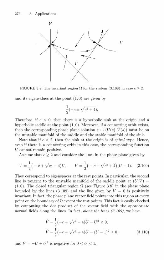
276 3. Applications
V
U
FIGURE 3.8. The invariant region Ω for the system (3.108) in case c ≥ 2.
and its eigenvalues at the point (1, 0) are given by
12(−c ±
√c2 + 4).
Therefore, if c > 0, then there is a hyperbolic sink at the origin and ahyperbolic saddle at the point (1, 0). Moreover, if a connecting orbit exists,then the corresponding phase plane solution s → (U(s), V (s)) must be onthe unstable manifold of the saddle and the stable manifold of the sink.
Note that if c < 2, then the sink at the origin is of spiral type. Hence,even if there is a connecting orbit in this case, the corresponding functionU cannot remain positive.
Assume that c ≥ 2 and consider the lines in the phase plane given by
V =12(
− c +√
c2 − 4)U, V =
12(
− c +√
c2 + 4)(U − 1). (3.109)
They correspond to eigenspaces at the rest points. In particular, the secondline is tangent to the unstable manifold of the saddle point at (U, V ) =(1, 0). The closed triangular region Ω (see Figure 3.8) in the phase planebounded by the lines (3.109) and the line given by V = 0 is positivelyinvariant. In fact, the phase plane vector field points into this region at everypoint on the boundary of Ω except the rest points. This fact is easily checkedby computing the dot product of the vector field with the appropriatenormal fields along the lines. In fact, along the lines (3.109), we have
V − 12(−c +
√c2 − 4)U = U2 ≥ 0,
V − 12(−c +
√c2 + 4)U = (U − 1)2 ≥ 0, (3.110)
and V = −U + U2 is negative for 0 < U < 1.
3.6 Origins of ODE: Partial Differential Equations 277
Suppose (as we will soon see) that the unstable manifold at the saddleintersects the region Ω. Then a solution that starts on this portion of theunstable manifold must remain in the region Ω for all positive time. Thus,the ω-limit set of the corresponding orbit is also in Ω. Because U ≤ 0 inΩ, there are no periodic orbits in Ω and no rest points in the interior of Ω.By the Poincare–Bendixson theorem, the ω-limit set must be contained inthe boundary of Ω. In fact, this ω-limit set must be the origin.
To complete the proof, we will show that the unstable manifold at thesaddle has nonempty intersection with the interior of Ω. To prove this fact,let us first recall that the unstable manifold is tangent to the line given bythe second equation in display (3.109). We will show that the tangency isquadratic and that the unstable manifold lies “above” this line. Our proofof this fact is more complicated than is necessary. However, the methodused can be generalized.
In the new coordinates given by
Z = U − 1, W = V,
the saddle rest point is at the origin for the equivalent first order system
Z = W, W = Z − cW + Z2.
The additional change of coordinates
Z = P, W = Q + αP := Q +12(−c +
√c2 + 4)P
transforms the system so that the unstable manifold of the saddle point istangent to the horizontal P -axis. We will show that the unstable manifoldis above this axis in some neighborhood of the origin; it then follows fromthe second formula in display (3.110) that the unstable manifold lies abovethe P -axis globally.
Note that the unstable manifold is given, locally at least, by the graphof a smooth function Q = h(P ) with h(0) = h′(0) = 0. Since this manifoldis invariant, we must have that Q = h′(P )P , and therefore, by an easycomputation,
P 2 − (c + α)h(P ) = h′(P )(h(P ) + αP ). (3.111)
The function h has the form h(P ) = βP 2 + O(P 3). By substitution of thisexpression into equation (3.111), we obtain the inequality
β = (3α + c)−1 > 0,
as required.
Much more can be said about the traveling wave solutions that we havejust found. A surprising fact is that all orbits of the PDE (3.107) start-ing with physically realistic initial conditions have as their ω-limit set the
278 3. Applications
traveling wave solution with wave speed c = 2. This fact was proved byAndrei N. Kolmogorov, Ivan G. Petrovskii, and Nikolai S. Piskunov [103](see also [15] and [21]). For a detailed mathematical account of travelingwave solutions see the book of Paul C. Fife [67] and also [132] and [162].
Exercise 3.45. Show that the PDE
ut − u2ux = uxx + u, x ∈ R, t ≥ 0
has a nonconstant solution that is periodic in both space and time.
3.6.4 First Order PDEConsider the special case of the model equation (3.80) where there is nodiffusion, but the medium moves with velocity field V ; that is, consider thedifferential equation
ut + γ gradu · V = f. (3.112)
This is an important example of a first order partial differential equation.Other examples are equations of the form
ut + (f(u))x = 0,
called conservation laws (see [162]), and equations of the form
St + H(Sq, q, t) = 0,
called Hamilton–Jacobi equations (see [10]). We will show how these PDEcan be solved using ordinary differential equations.
Let us consider the case of one space variable; the general case is similar.If γ = 1, then the equation (3.112) is given by
ut + v(x, t)ux = f(u, x, t),
or, with a redefinition of the names of the functions, it has the more generalform
f(x, y, u)ux + g(x, y, u)uy = h(x, y, u). (3.113)
We will “solve” the PDE (3.113) using the following basic idea: If thegraph G of a function z = u(x, y) is an invariant manifold for the first ordersystem
x = f(x, y, z), y = g(x, y, z), z = h(x, y, z), (3.114)
then u is a solution of the PDE (3.113). Indeed, using the results of Sec-tion 1.7 and the fact that
(x, y) → (x, y, u(x, y), ux(x, y), uy(x, y),−1)
3.6 Origins of ODE: Partial Differential Equations 279
is a normal vector field on G, it follows that the manifold G is invariantif and only if the dot product of the vector field associated with the sys-tem (3.114) and the normal field is identically zero; that is, if and only ifequation (3.113) holds. The orbits of the system (3.114) are called charac-teristics of the PDE (3.113).
Perhaps it is possible to find an invariant manifold for the first ordersystem (3.114) by an indirect method. However, we can also construct theinvariant manifold directly from appropriate initial data. To see how thisis done, let us suppose that we have a curve in space given by γ : R → R
3
such that in coordinates
γ(s) = (γ1(s), γ2(s), γ3(s)).
This curve is called noncharacteristic at γ(0) if
f(γ(0))γ2(0) − g(γ(0))γ3(0) = 0.
Let ϕt denote the flow of the system (3.114), and define H : R2 → R
3 by
(s, t) → ϕt(γ(s)). (3.115)
Also, define H : R2 → R
2 by projection of the image of H onto its first twocomponents. More precisely, let e1, e2, e3 be the usual basis vectors for R
3
and let the usual inner product be denoted by angle brackets. Then H isgiven by
(s, t) → (〈ϕt(γ(s)), e1〉, 〈ϕt(γ(s)), e2〉).
We will show that H is locally invertible at γ(0). For this, compute
DH(0, 0)e1 =d
dτH(τ, 0)
∣∣∣τ=0
=d
dτ(γ1(s), γ2(s))
∣∣∣τ=0
= (γ1(0), γ2(0)),
and similarly
DH(0, 0)e2 = (f(γ1(0)), g(γ2(0))).
Because the curve γ is noncharacteristic at γ(0), the matrix representationof DH(0, 0) has nonzero determinant and is therefore invertible. By theinverse function theorem, H is locally invertible at the origin.
Using the local inverse of H, let us note that
H(H−1(x, y)) = (x, y,H3(H−1(x, y))).
280 3. Applications
In other words, if u(x, y) := H3(H−1(x, y)), then the surface given bythe range of H is locally the graph of the function u. This completes theconstruction of u; it is a local solution of the PDE (3.113).
We have now proved that if we are given initial data on a noncharacter-istic curve, then there is a corresponding local solution of the PDE (3.113).Also, we have a method to construct such a solution.
As an example, let us consider the model equation
uτ + a sin(ωτ)ux = u − u2, 0 ≤ x ≤ 1, t ≥ 0
with initial data u(x, 0) = u0(x) defined on the unit interval. A phenomeno-logical interpretation of this equation is that u is the density of a specieswith logistic growth in a moving medium that is changing direction withfrequency ω and amplitude a. We have used τ to denote the time parameterso that we can write the first order system for the characteristics in theform
τ = 1, x = a sin(ωτ), z = z − z2.
To specify the initial data, let us define the noncharacteristic curve givenby s → (0, s, u0(s)). Then, after solving the first order system and usingthe definition (3.115), we have that
H(s, t) =(t, s +
a
µ(1 − cos µt),
etu0(s)1 + u0(s)(et − 1)
).
Also, because H−1 is given explicitly by
H−1(τ, x) = (τ, x − a
µ(1 − cos µτ)),
we have the solution
u(x, t) =eτu0(x − a
µ (1 − cos µτ))
1 + (eτ − 1)u0(x − aµ (1 − cos µτ))
. (3.116)
What does our model predict? For example, if the initial condition isgiven by a positive function u0, then the ω-limit set of the correspondingsolution of the PDE is the constant function u ≡ 1, the solution corre-sponding to no drift. However, if the initial population is distributed sothat some regions have zero density, then the fate of the initial populationis more complicated (see Exercise 3.46).
Exercise 3.46. What long term behavior for the corresponding model equationis predicted by the solution (3.116)? How does your answer depend on the choiceof u0, a, and ω?
3.6 Origins of ODE: Partial Differential Equations 281
Exercise 3.47. Solve the PDE xux + yuy = 2u with u prescribed on the unitcircle. Hint: Define the noncharacteristic curve
s → (cos s, sin s, h(cos s, sin s)).
Exercise 3.48. Find solutions of the PDE xux − yuy = 2u. How should thedata be prescribed?
Exercise 3.49. A function U that is constant along the orbits of an ordinarydifferential equation is called an invariant function, or a first integral. In symbols,if we have a differential equation x = f(x) with flow ϕt, then U is invariantprovided that U(φt(x)) = U(x) for all x and t for which the flow is defined. Showthat U is invariant if and only if 〈grad U(x), f(x)〉 ≡ 0. Equivalently, the Liederivative of U in the direction of the vector field given by f vanishes. Considerthe differential equation
θ = 1, φ = α
where α ∈ R. Also, consider both θ and φ as angular variables so that thedifferential equation can be viewed as an equation on the torus. Give necessaryand sufficient conditions on α so that there is a smooth invariant function definedon the torus.
Exercise 3.50. A simple example of a conservation law is the (nonviscous)Burgers’ equation ut + uux = 0. Burgers’ equation with viscosity is given by
ut + uux =1
Reuxx
where Re is called the Reynold’s number. This is a simple model that incorporatestwo of the main features in fluid dynamics: convection and diffusion. Solve thenonviscous Burgers’ equation with initial data u(x, 0) = (1 − x)/2 for −1 <x < 1. Note that the solution cannot be extended for all time. This is a generalphenomenon that appears in the study of conservation laws that is related to theexistence of shock waves (see [162]). Also, consider the viscous Burgers’ equationon the same interval with the same initial data and with boundary conditions
u(−1, t) = 1, u(1, t) = 0.
How can we find Galerkin approximations? The problem is that with the nonho-mogeneous boundary conditions, there is no vector space of functions that satisfythe boundary conditions. To overcome this problem, we can look for a solutionof our problem in the form
u(x, t) = v(x, t) +12(1 − x)
where v satisfies the equation
vt + (v +12(1 − x))(vx − 1
2) = vxx
and Dirichlet boundary conditions. Determine the Galerkin approximations us-ing trigonometric trial functions. Use a numerical method to solve the resulting
282 3. Applications
differential equations, and thus approximate the solution of the PDE. For a nu-merical analyst’s approach to this problem, consider the Galerkin approximationswith respect to the “test function basis” of Chebyshev polynomials given by
T0(x) = 1, T1(x) = x, T2(x) = 2x2 − 1
and
Tn+1(x) = 2xTn(x) − Tn−1(x).
The Chebyshev polynomials are orthogonal (but not orthonormal) with respectto the inner product defined by
〈f, g〉 :=∫ 1
−1f(x)g(x)(1 − x2)−1/2 dx.
Moreover, the Chebyshev polynomials do not satisfy the boundary conditions.However, proceed as follows: Look for a Galerkin approximation in the form
un(x, t) =n∑
i=1
ci(t)Tn−1(x),
but only construct the corresponding system of differential equations for
c1, . . . , cn−2.
Then, define the last two coefficients so that the boundary conditions are satisfied(see [69]). Compare numerical results. Finally, note that Burgers’ equation can,in principle, be solved explicitly by the Hopf–Cole transformation. In fact, if u isa solution of Burgers’ equation and ψ is defined so that ψx = u, then ψ is definedup to a function that depends only on the time variable. An appropriate choiceof the antiderivative satisfies the equation
ψt +12ψ2
x =1
Reψxx.
If φ is defined by the equation ψ = −(2/Re)φ, then
φt =1
Reφxx.
Thus, solutions of the heat equation can be used to construct solutions of Burgers’equation. The fact that Burgers’ equation can be solved explicitly makes this PDEa very useful candidate for testing numerical codes.
4Hyperbolic Theory
The chapter is an introduction to the theory of hyperbolic structures in dif-ferential equations. The basic idea might be called “the principle of hyper-bolic linearization.” Namely, if the linearized flow of a differential equationhas “no eigenvalues with zero real parts,” then the nonlinear flow behaveslocally like the linear flow. This idea has far-reaching consequences thatare the subject of many important and useful mathematical results. Herewe will discuss two fundamental theorems: the center and stable manifoldtheorem for a rest point and Hartman’s theorem.
4.1 Invariant Manifolds
One of the important results in the theory of ordinary differential equationsis the stable manifold theorem. This and many closely related results, forexample, the center manifold theorem, form the foundation for analyzingthe dynamical behavior of a dynamical system in the vicinity of an invariantset. In this section we will consider some of the theory that is used toprove such results, and we will prove the existence of invariant manifoldsrelated to the simplest example of an invariant set, namely, a rest point.However, the ideas that we will discuss can be used to prove much moregeneral theorems. In fact, some of the same ideas can be used to provethe existence and properties of invariant manifolds for infinite dimensionaldynamical systems.
284 4. Hyperbolic Theory
The concept of the invariant manifolds for rest points arises from thestudy of linear systems. Recall that if A is a linear map of R
n, then thespectrum of A splits naturally—from the point of view of stability theory—into three subsets: the eigenvalues with negative, zero, or positive real parts.After a linear change of coordinates that transforms A to its real Jordannormal form, we find that the differential equation u = Au decouples intoa system
x = Sx, y = Uy, z = Cz
where (x, y, z) ∈ Rk × R
× Rm with k + + m = n, and where S, U and C
are linear operators whose eigenvalues have all negative, zero, and positivereal parts, respectively. The subspace R
k ⊂ Rn is called the stable manifold
of the rest point at the origin for the original system u = Au, the subspaceR
is called the unstable manifold, and the subspace Rm is called the center
manifold.We proved previously, in Theorem 2.34, that there are constants K > 0,
a > 0 and b > 0 such that if ξ ∈ Rk and ζ ∈ R
n, then
‖x(t, ξ)‖ = ‖etSξ‖ ≤ Ke−at‖ξ‖, t ≥ 0,
‖y(t, ζ)‖ = ‖etUζ‖ ≤ Kebt‖η‖, t ≤ 0, (4.1)
where t → x(t, ξ) is the solution of the differential equation x = Sx withthe initial condition x(0, ξ) = ξ, and y is defined similarly. Here, ‖ ‖ isan arbitrary norm on R
n. There are no such exponential estimates on thecenter manifold.
An analysis of the dynamics on the center manifold, when it exists, isoften one of the main reasons for finding a center manifold in the first place.In this regard, let us recall that the flow of a nonlinear system near a restpoint where the linearization has an eigenvalue with zero real part is notdetermined by the linearized flow. For example, the linearization at a restpoint of a planar system might have a center, whereas the correspondingrest point for the nonlinear system is a sink or a source. In this case thecenter manifold at the rest point is an open subset of the plane. As thisexample shows, we can expect the most complicated (and most interesting)dynamics near a nonhyperbolic rest point to occur on a corresponding cen-ter manifold. If a center manifold has dimension less than the dimensionof the phase space, then the most important dynamics can be studied byconsidering the restriction of the original system to a center manifold. Toillustrate, let us imagine a multidimensional system that has a rest pointwith a codimension two stable manifold and a two-dimensional center man-ifold. Then, as we will see, the orbits of the nonlinear system are all locallyattracted to the center manifold, and therefore the nontrivial dynamics canbe determined by studying a planar system. This “center manifold reduc-tion” to a lower dimensional system is one of the main applications of thetheory.
4.1 Invariant Manifolds 285
The stable manifold theorem states that if the linear system u = Auhas no center manifold, then the nonlinear system u = Au + H(u), whereH : R
n → Rn with H(0) = 0 and DH(0) = 0, has stable and unstable
manifolds corresponding to the stable and unstable manifolds of the linearsystem. These manifolds are invariant sets that contain the rest point atthe origin, and they have the same dimensions as the corresponding linearmanifolds. In fact, the corresponding linear manifolds are their tangentspaces at the rest point. Moreover, the flow restricted to the stable and theunstable manifolds has exponential (hyperbolic) estimates similar to theinequalities in display (4.1)
There are several different methods available to prove the existence ofinvariant manifolds. Each of these methods has technical as well as concep-tual advantages and disadvantages. Here we will use the Lyapunov–Perronmethod. The basic idea is to determine the invariant manifold as the graphof a function that is obtained as the fixed point of an integral operator ona Banach space. An alternative method based on the “graph transform”is also very important (see [94] and [151]). The Lyapunov–Perron methodhas wide applicability and it can be used to prove very general theorems.While the graph transform method is perhaps even more far-reaching, themain reason for using the Lyapunov–Perron method here is that the theoryillustrates many useful ODE techniques.
For the invariant manifold theory that we will discuss, it is not neces-sary to assume the existence of an infinitesimally hyperbolic linearization.Instead, it suffices to assume that the spectrum of the linearization has aspectral gap; that is, the spectrum is separated into two vertical strips inthe complex plane such that the maximum of the real parts of the eigenval-ues in the left hand strip is strictly less than the minimum of the real partsof the eigenvalues in the right hand strip. This hypothesis is exactly theright condition required to apply the Lyapunov–Perron method to obtainthe existence of an invariant manifold. The stable, unstable, and centermanifold theorems are easily obtained as corollary results.
We will use the notation C1 as a prefix to denote spaces of continuouslydifferentiable functions. If f is such a function, then let ‖f‖1 denote theC1-norm given by the sum of the supremum norm of f and the supremumnorm of its derivative Df , where the supremum is taken over the domainof definition of the function.
The next theorem is the main result of this section. It states the existenceof a smooth global invariant manifold at a rest point of a nonlinear system,provided that the linearization of the system at the rest point has a spectralgap and the nonlinear remainder terms are sufficiently small. The proofof this theorem is quite long, but it is not too difficult to understand.The idea is to set up a contraction in an appropriate Banach space ofcontinuous functions so that the fixed point of the contraction is a functionwhose graph is the desired invariant manifold. Then the fiber contraction
286 4. Hyperbolic Theory
principle is applied to show that this function is smooth. The proof usesmany important ODE techniques that are well worth learning.
Theorem 4.1. Suppose that S : Rk → R
k and U : R → R
are lineartransformations such that all eigenvalues of S have real part less than a,all eigenvalues of U have real part greater than b, and a < b. If F ∈C1(Rk × R
, Rk) and G ∈ C1(Rk × R, R) are such that F (0, 0) = 0,
DF (0, 0) = 0, G(0, 0) = 0, DG(0, 0) = 0, and such that ‖F‖1 and ‖G‖1are sufficiently small, then there is a unique function α ∈ C1(Rk, R) withthe following properties
α(0) = 0, Dα(0) = 0, supξ∈Rk
‖Dα(ξ)‖ < ∞,
whose graph, namely the set
W (0, 0) = (x, y) ∈ Rk × R
: y = α(x),
is an invariant manifold for the system of differential equations given by
x = Sx + F (x, y), y = Uy + G(x, y). (4.2)
Moreover, if (ξ, α(ξ)) ∈ W (0, 0), then for each λ > a there is a constantC > 0 such that the solution t → (x(t), y(t)) of the system (4.2) with initialcondition (ξ, α(ξ)) satisfies the exponential estimate
‖x(t)‖ + ‖y(t)‖ ≤ Ceλt‖ξ‖.
Proof. We will use several Banach spaces and several different norms. Theproofs that these spaces with the indicated norms are indeed Banach spacesare left to the reader. However, we will outline a proof for one of the spaces.
Let C0(RN , RM ) denote the linear space of all continuous functions
f : RN → R
M ,
and let us use it to define the following Banach spaces: C0(RN , RM ), theset of all functions f ∈ C0(RN , RM ) such that f(0) = 0 and
‖f‖0 = supξ∈RN
‖f(ξ)‖ < ∞;
C1(RN , RM ), the set of all continuously differentiable functions
f ∈ C0(RN , RM )
such that f(0) = 0, Df(0) = 0, and
‖f‖1 = ‖f‖0 + ‖Df‖0 < ∞;
4.1 Invariant Manifolds 287
and E0(RN , RM ), the set of all functions f ∈ C0(RN , RM ) such that f(0) =0 and
‖f‖E = sup‖f(ξ)‖‖ξ‖ : ξ ∈ R
N , ξ = 0 < ∞.
Also, for f ∈ C0(RN , RM ), let the Lipschitz constant of f be denoted by
Lip(f) := supξ =η
‖f(ξ) − f(η)‖‖ξ − η‖
whenever the indicated supremum is finite.Proposition A: The space E0(RN , RM ) with the E-norm is a Banach
space.To prove the proposition, let us assume for the moment that if fn∞
n=1is a sequence in E0(RN , RM ) that converges in the E-norm to a functionf : R
N → RM , then the sequence converges uniformly on compact subsets
of RN . Using the usual theorems on uniform convergence, it follows from
this fact that the limit function f is continuous on RN . Also, there is a
sufficiently large integer n such that ‖f − fn‖E < 1. Thus, for this choiceof n, we have that
‖f‖E ≤ ‖f − fn‖E + ‖fn‖E < 1 + ‖fn‖,
and as a result we see that the E-norm of f is bounded.To show that E0(RN , RM ) is a Banach space, we must show that it is
complete. To this end, suppose that the above sequence is Cauchy. We willshow that the sequence converges to a function f : R
N → RM with f(0) =
0. By the facts claimed above, we must then have that f ∈ E0(RN , RM ),as required.
Let us define a function f : RN → R
M . First, set f(0) = 0. If ξ ∈ RN is
not the zero vector, let ε > 0 be given and note that there is an integer Jsuch that
‖fm(ξ) − fn(ξ)‖‖ξ‖ <
ε
‖ξ‖whenever m and n exceed J . Thus, the sequence fn(ξ)∞
n=1 is a Cauchysequence in R
M , and hence it has a limit that we define to be f(ξ).We claim that the sequence fn∞
n=1 converges to the function f in theE-norm. To prove the claim, let ε > 0 be given. There is an integer J , asbefore, such that, if ξ = 0, then
‖fn(ξ) − fp(ξ)‖‖ξ‖ <
ε
2
whenever the integers n and p exceed J . It follows that if ξ ∈ RN , including
ξ = 0, then the inequality
‖fn(ξ) − fp(ξ)‖ ≤ ε
2‖ξ‖
288 4. Hyperbolic Theory
holds whenever n and p exceed J . Using this fact, we have the followingestimates
‖fn(ξ) − f(ξ)‖ ≤ ‖fn(ξ) − fp(ξ)‖ + ‖fp(ξ) − f(ξ)‖
≤ ε
2‖ξ‖ + ‖fp(ξ) − f(ξ)‖.
If we now pass to the limit as p → ∞, we find that, for all ξ ∈ RN ,
‖fn(ξ) − f(ξ)‖‖ξ‖ ≤ ε
2< ε
whenever n exceeds J . Thus, we have that ‖fn − f‖E < ε whenever nexceeds J , and therefore the sequence converges to f in the E-norm.
To finish the proof, we must show that convergence in the E-norm isuniform on compact sets. To this end, suppose that fn∞
n=1 converges tof in the E-norm, let K be a compact subset of R
N , and let ε > 0 be given.Also, let us define r := supξ∈K ‖ξ‖. There is an integer J such that if ξ = 0,then
‖fn(ξ) − f(ξ)‖‖ξ‖ <
ε
r + 1
whenever n exceeds J . Hence, as before, if ξ ∈ K, then
‖fn(ξ) − f(ξ)‖ ≤ ε
r + 1‖ξ‖ ≤ ε
r
r + 1< ε
whenever n exceeds J . It follows that the convergence is uniform on thecompact set K. This completes the proof of Proposition A.
Let us define two subsets of the Banach spaces defined above as follows:
B0ρ(RN , RM ) := f ∈ E(RN , RM ) : Lip(f) ≤ ρ,
B1δ(RN , RM ) := f ∈ C1(RN , RM ) : ‖f‖1 < δ.
The set B0ρ(RN , RM ) is a closed (in fact, compact) subset of E(RN , RM ),
while the set B1δ(RN , RM ) is an open subset of C1(RN , RM ). Moreover, the
set B0ρ(RN , RM ) is a complete metric space with respect to the metric given
by the E-norm.Fix ρ > 0. If δ > 0, F ∈ B1
δ(Rk × R, RM ), and α ∈ B0
ρ(Rk, R), then thedifferential equation
x = Sx + F (x, α(x)) (4.3)
has a continuous flow. In fact, for each ξ ∈ Rk, there is a solution t →
x(t, ξ, α) such that x(0, ξ, α) = ξ and such that (t, ξ, α) → x(t, ξ, α) is acontinuous function.
4.1 Invariant Manifolds 289
To compress notation, let us define
χ(t) := x(t, ξ, α)
and note that the function t → χ(t) is defined for all t ≥ 0. In fact, fromthe hypotheses of the theorem, there is a constant K > 0 such that for allξ ∈ R
k and for all ν ∈ R, we have the following exponential estimates
‖etSξ‖ ≤ Keat‖ξ‖, ‖e−tUν‖ ≤ Ke−bt‖ν‖
for all t ≥ 0. The proof of these estimates under the spectral gap conditionis similar to the proof of Theorem 2.34.
Using the fact that ‖DF‖0 < δ and the mean value theorem, we havethat
‖F (x, y)‖ = ‖F (x, y) − F (0, 0)‖ ≤ δ(‖x‖ + ‖y‖)
where we are using the sum of the norms on each factor for the norm onthe cross product space R
k × R. Also, after obtaining a similar estimate
for α, and combining these estimates, it follows that
‖F (x, α(x))‖ ≤ δ(1 + ρ)‖x‖.
By an application of the variation of constants formula (2.37), the func-tion χ satisfies the integral equation
χ(t) = etSξ +∫ t
0e(t−τ)SF (χ(τ), α(χ(τ))) dτ (4.4)
from which we obtain the estimate
‖χ(t)‖ ≤ Keat‖ξ‖ +∫ t
0Kδ(1 + ρ)ea(t−τ)‖χ(τ)‖ dτ.
Equivalently, we have
e−at‖χ(t)‖ ≤ K‖ξ‖ +∫ t
0Kδ(1 + ρ)e−aτ‖χ(τ)‖ dτ,
and by an application of Gronwall’s inequality, we obtain the estimate
‖x(t, ξ)‖ = ‖χ(t)‖ ≤ K‖ξ‖e(Kδ(1+ρ)+a)t. (4.5)
In particular, the solution t → x(t, ξ) does not blow up in finite time.Hence, it is defined for all t ≥ 0.
For α ∈ B0ρ(Rk, R) and G ∈ B1
δ(Rk × R, R), if the graph
Mα := (x, y) ∈ Rk × R
: y = α(x)
290 4. Hyperbolic Theory
is an invariant set for the system (4.2), then the function
t → y(t, ξ, α) := α(x(t, ξ, α))
is a solution of the differential equation
y = Uy + G(x, y) (4.6)
with initial condition y(0, ξ, α) = α(ξ). Equivalently, by variation of pa-rameters and with the notational definition γ(t) := y(t, ξ, α), we have that
e−tUγ(t) − α(ξ) =∫ t
0e−τUG(χ(τ), α(χ(τ))) dτ.
Note that
‖e−tUγ(t)‖ ≤ Ke−btρ‖χ(t)‖ ≤ K2ρ‖ξ‖e(Kδ(1+ρ)+a−b)t. (4.7)
Thus, using the fact that a − b < 0, if we choose δ so that
0 < δ <b − a
K(1 + ρ),
then limt→∞ ‖e−tUγ(t)‖ = 0 and
α(ξ) = −∫ ∞
0e−τUG(χ(τ), α(χ(τ))) dτ. (4.8)
Conversely, if α ∈ B0ρ(Rk, R) satisfies the integral equation (4.8), then
the graph of α is an invariant manifold. To see this, consider a point (ξ, α(ξ))on the graph of α, and redefine χ(t, ξ) := x(t, ξ, α) and γ(t) := α(χ(t, ξ)).We will show that γ is a solution of the differential equation (4.6). Indeed,from the integral equation (4.8), we have that
d
dt
(e−tUγ(t)
)= − d
dt
∫ ∞
0e−(t+τ)UG(χ(τ, χ(t, ξ)), α(χ(τ, χ(t, ξ)))) dτ
= − d
dt
∫ ∞
0e−(t+τ)UG(χ(τ + t, ξ), α(χ(τ + t, ξ))) dτ
= − d
dt
∫ ∞
t
e−sUG(χ(s, ξ), α(χ(s, ξ))) ds
= e−tUG(χ(t, ξ), γ(t)).
In other words,
e−tU γ(t) − e−tUUγ(t) = e−tUG(χ(t, ξ), γ(t)),
and therefore γ is a solution of the differential (4.6), as required.
4.1 Invariant Manifolds 291
Proposition B: If ρ > 0 is given, if δ > 0 is sufficiently small, and ifF ∈ B1
δ(Rk × R, Rk) and G ∈ B1
δ(Rk × R, R), then the Lyapunov–Perron
operator Λ defined by
Λ(α)(ξ) := −∫ ∞
0e−tUG(x(t, ξ, α), α(x(t, ξ, α))) dt
is a contraction on the complete metric space B0ρ(Rk, R).
Let us first prove that the range of Λ is in the space B0ρ(Rk, R). For this,
consider ξ, η ∈ Rk, and note that
‖Λ(α)(ξ) − Λ(α)(η)‖ ≤ K(1 + ρ)‖G‖1
∫ ∞
0e−bt‖x(t, ξ, α) − x(t, η, α)‖ dt.
Using the integral equation (4.4), we have the estimate
‖x(t, ξ, α) − x(t, η, α)‖
≤ Keat‖ξ − η‖ +∫ t
0K‖F‖1(1 + ρ)ea(t−τ)‖x(τ, ξ, α) − x(τ, η, α)‖ dτ.
After multiplying both sides of this last inequality by e−at and applyingGronwall’s inequality, we have that
‖x(t, ξ, α) − x(t, η, α)‖ ≤ K‖ξ − η‖e(K‖F‖1(1+ρ)+a)t. (4.9)
Returning to the original estimate, let us substitute the inequality (4.9)and carry out the resulting integration to obtain the inequality
‖Λ(α)(ξ) − Λ(α)(η)‖ ≤ K2δ(1 + ρ)b − a − Kδ(1 + ρ)
‖ξ − η‖. (4.10)
If ‖F‖1 and ‖G‖1 are sufficiently small, that is, if δ > 0 is sufficientlysmall, then it follows that Λ(α) is a Lipschitz continuous function withLipschitz constant less than ρ. In fact, it suffices to take
0 < δ < min b − a
K(1 + ρ),
(b − a)ρK(1 + ρ)(K + ρ)
.
If δ > 0 is less than the first element in the brackets, then the denominatorof the fraction in inequality (4.10) is positive. If δ > 0 is less than the secondelement, then the fraction is less than ρ. Moreover, if we take ξ = 0, thenx(t, 0, α) ≡ 0 is the corresponding solution of the differential equation (4.3),and it follows that Λ(α)(0) = 0.
To show that ‖Λ(α)‖E < ∞, let us use the estimate (4.10) with η = 0 toget
supξ =0
‖Λ(α)(ξ)‖‖ξ‖ ≤ K2δ(1 + ρ)
b − a − Kδ(1 + ρ)< ∞.
292 4. Hyperbolic Theory
This completes the proof that Λ is a transformation of the complete metricspace B0
ρ(Rk, R) into itself.It remains to show that Λ is a contraction. Using the fact that ‖G‖1
is finite; the fact that the Lipschitz constant for all functions in the spaceB0
ρ(Rk, R) does not exceed ρ; and the definition that the norm on the crossproduct R
k×R is the sum of the Euclidean norms on the factors, we obtain
the inequalities
‖Λ(α)(ξ) − Λ(β)(ξ)‖
≤ K
∫ ∞
0e−bt‖G(x(t, ξ, α), α(x(t, ξ, α))) − G(x(t, ξ, β), β(x(t, ξ, β)))‖ dt
≤ K‖G‖1
∫ ∞
0e−bt(‖x(t, ξ, α) − x(t, ξ, β)‖
+ ‖α(x(t, ξ, α)) − α(x(t, ξ, β))‖ + ‖α(x(t, ξ, β)) − β(x(t, ξ, β))‖ dt
≤ K‖G‖1
∫ ∞
0e−bt((1 + ρ)‖x(t, ξ, α) − x(t, ξ, β)‖
+ ‖α − β‖E‖x(t, ξ, β)‖) dt. (4.11)
To estimate the terms in the integrand of the last integral in the dis-play (4.11), let us use the integral equation (4.4) to obtain the estimate
‖x(t, ξ, α) − x(t, ξ, β)‖ ≤
K
∫ t
0ea(t−τ)‖F (x(τ, ξ, α), α(x(τ, ξ, α))) − F (x(τ, ξ, β), β(x(τ, ξ, β)))‖ dτ.
Then, by proceeding exactly as in the derivation of the estimate (4.11), itis easy to show that
‖x(t, ξ, α) − x(t, ξ, β)‖
≤ K‖F‖1
∫ t
0ea(t−τ)((1 + ρ)‖x(τ, ξ, α) − x(τ, ξ, β)‖ dτ
+ K‖F‖1‖α − β‖E∫ t
0‖x(τ, ξ, β)‖) dτ.
After inserting the inequality (4.5), integrating the second integral, andmultiplying both sides of the resulting inequality by e−at, we find that
e−at‖x(t, ξ, α) − x(t, ξ, β)‖ ≤∫ t
0K‖F‖1e
−aτ‖x(τ, ξ, α) − x(τ, ξ, β)‖ dτ
+K‖F‖1‖ξ‖δ(1 + ρ)
‖α − β‖E(eKδ(1+ρ)t − 1
).
Then, an application of Gronwall’s inequality followed by some algebraicmanipulations can be used to show the estimate
‖x(t, ξ, α) − x(t, ξ, β)‖ ≤ K
1 + ρ‖α − β‖E‖ξ‖e(2Kδ(1+ρ)+a)t.
4.1 Invariant Manifolds 293
Returning to the main estimate, if we insert the last inequality as wellas the inequality (4.5), then an integration together with some obviousmanipulations yields the estimate
‖Λ(α) − Λ(β)‖E ≤ 2K2δ
b − a − 2Kδ(1 + ρ)‖α − β‖E .
Moreover, if
0 < δ < min b − a
2K(1 + ρ),
b − a
2K(K + 1 + ρ)
,
then Λ has a contraction constant strictly less than one, as required.Taking into account all the restrictions on δ, if
0 < δ <b − a
Kmin
ρ
(1 + ρ)(K + ρ),
12(1 + ρ)
,1
2(K + 1 + ρ)
,
then the Lyapunov–Perron operator has a fixed point whose graph is aLipschitz continuous invariant manifold that passes through the origin.This completes the proof of Proposition B.
Let us apply the fiber contraction principle to prove the smoothness ofthe invariant manifold that corresponds to the function α obtained as thefixed point of the Lyapunov–Perron operator. To this end, let us followthe prescription outlined after the proof of the fiber contraction theorem(Theorem 1.176).
The space of “candidates for the derivatives of functions in B0ρ(Rk, R)”
is, in the present case, the set F = C(Rk, L(Rk, R)) of all bounded con-tinuous functions Φ that map R
k into the bounded linear maps from Rk
into R with Φ(0) = 0 and with the norm
‖Φ‖F := supξ∈Rk
‖Φ(ξ)‖,
where ‖Φ(ξ)‖ denotes the usual operator norm of the linear transformationΦ(ξ). Also, let Fρ denote the closed ball in F with radius ρ, that is,
Fρ := Φ ∈ F : ‖Φ‖ ≤ ρ
where ρ > 0 is the number chosen in the first part of the proof.Proposition C: Suppose that β ∈ B0
ρ(Rk, R), the function t → x(t, ξ, β)is the solution of the differential equation (4.3) with parameter β and initialcondition x(0, ξ, β) = ξ, and Φ ∈ Fρ. If ‖F‖1 and ‖G‖1 are both sufficientlysmall, then Ψ given by
Ψ(β,Φ)(ξ) := −∫ ∞
0e−tU [Gx(x(t, ξ, β), β(x(t, ξ, β)))W (x(t, ξ, β))
+ Gy(x(t, ξ, β), β(x(t, ξ, β)))Φ(x(t, ξ, β))W (x(t, ξ, β))] dt
(4.12)
294 4. Hyperbolic Theory
where
W (t, ξ, β) :=∫ t
0e(t−s)S [Fx(x(s, ξ, β), β(x(s, ξ, β)))W (x(s, ξ, β))
+Fy(x(s, ξ, β), β(x(s, ξ, β)))Φ(x(s, ξ, β))W (x(s, ξ, β))] ds
(4.13)
defines a function from B0ρ ×Fρ to Fρ. If, in addition, β is continuously dif-
ferentiable and if Λ denotes the Lyapunov–Perron operator, then DΛ(β) =Ψ(β, Dβ).
To prove the first statement of the proposition, let us begin by showingthat the indefinite integral in the definition of Ψ is convergent. Using thehypotheses of the theorem and estimating in the usual manner, we havethat
‖Φ(β,Φ)(ξ)‖ ≤∫ ∞
0Ke−bt‖G‖1(1 + ρ)‖W (t, ξ, β)‖ dt. (4.14)
An upper bound for ‖W (t, ξ, β)‖ is easily obtained from the integralequation (4.13). In fact, estimating once again in the usual manner, wehave
‖W (t, ξ, β)‖ ≤ Keat +∫ t
0K‖F‖1(1 + ρ)e(t−s)a‖W (s, ξ, β)‖ dt.
After multiplying both sides of this last inequality by e−at and then apply-ing Gronwall’s inequality, we obtain the estimate
‖W (t, ξ, β)‖ ≤ Ke(K‖F‖1(1+ρ)+a)t. (4.15)
If the inequality (4.15) is inserted into the estimate (4.14), with
‖F‖1 ≤ δ <b − a
K(1 + ρ),
and the resulting integral is evaluated, then we have that
‖Ψ(β,Φ)(ξ)‖ ≤ K2‖G‖1(1 + ρ)b − a − Kδ(1 + ρ)
. (4.16)
Thus, the original integral converges. Moreover, if the quantity ‖G‖1 issufficiently small—the upper bound
‖G‖1 ≤ δ ≤ ρ(b − a − Kδ(1 + ρ))K2(1 + ρ)
will suffice—then
‖Ψ(β,Φ)(ξ)‖ ≤ ρ.
4.1 Invariant Manifolds 295
Finally, it is easy to check that Ψ(β,Φ)(0) = 0. Therefore, Ψ(β,Φ) ∈ Fρ,as required.
If β is continuously differentiable, then the solution t → x(t, ξ, β) of thedifferential equation (4.3) given by
x = Sx + F (x, β(x))
is continuously differentiable by Theorem 1.184. Moreover, if we defineΦ := Dβ, then W (t, ξ, β) := xξ(t, ξ, β) (the solution of the first variationalequation of the differential equation (4.3)) is the corresponding solutionof the integral equation (4.13). In this case, the integrand of the integralexpression for Λ(β)(ξ) is clearly a differentiable function of ξ with deriva-tive exactly the integrand of the integral expression for Ψ(β, Dβ)(ξ). As wehave shown above, this integrand is bounded above by an integrable func-tion. Thus, differentiation under the integral sign is justified, and in fact,DΛ(β) = Ψ(β, Dβ), as required. This completes the proof of the proposi-tion.
Let us show that
Λ : B0ρ(Rk, R) × Fρ → B0
ρ(Rk, R) × Fρ
given by (β,Φ) → (Λ(β), Ψ(β,Φ)), is a fiber contraction. For this, fix β ∈B0
ρ(Rk, R) and consider the estimates (analogous to those made previously)given by
‖Ψ(β,Φ1)(ξ)−Ψ(β,Φ2)(ξ)‖
≤∫ ∞
0e−bt(‖GxW1 + GyΦ1W1 − GxW2 − GyΦ2W2)‖ dt
≤∫ ∞
0e−bt‖G‖1(‖W1 − W2‖ + ‖Φ1W1 − Φ2W2‖ dt
≤∫ ∞
0e−bt‖G‖1(‖W1 − W2‖ + ‖Φ1‖‖W1 − W2‖
+ ‖Φ1 − Φ2‖‖W2‖) dt (4.17)
≤∫ ∞
0e−bt‖G‖1((1 + ρ)‖W1 − W2‖ + ‖Φ1 − Φ2‖F‖W2‖) dt,
where, for notational convenience, the arguments of the functions in theintegrands have been suppressed.
Let us estimate ‖W1 −W2‖. The upper estimates are obtained in a man-ner that is completely analogous to the estimate just completed; in fact,
‖W1(t, ξ, α)−W2(t, ξ, β)‖
≤∫ t
0K‖F‖1(1 + ρ)ea(t−s)‖W1(s, ξ, α) − W2(s, ξ, β)‖ ds
+ K‖F‖1‖Φ1 − Φ2‖F∫ t
0ea(t−s)‖W2(s, ξ, β)‖ ds.
296 4. Hyperbolic Theory
Now, insert the inequality (4.15) into the second integral, carry out theintegration in the second integral, multiply both sides of the resulting in-equality by e−at, and apply Gronwall’s inequality to show the estimate
‖W1(t, ξ, α) − W2(t, ξ, β)‖ ≤ K
1 + M‖Φ1 − Φ2‖Fe(2K‖F‖1(1+ρ)+a)t. (4.18)
If we insert the inequalities (4.15) and (4.18) into the estimate (4.17),then, after integration of the resulting integrals and some obvious manip-ulation, we find that
‖Ψ(β,Φ1)(ξ) − Ψ(β,Φ2)(ξ)‖ ≤ 2K2‖F‖1
b − a − 2K‖G‖1(1 + ρ)‖Φ1 − Φ2‖F .
(4.19)
Thus, if
0 < δ <b − a
2K(K + 1 + ρ),
‖F‖1 ≤ δ, and ‖G‖1 ≤ δ, then
0 <2K2‖F‖1
b − a − 2K‖G‖1(1 + ρ)< 1,
and therefore Λ is a fiber contraction.Let us define (φ0, Φ0) = (0, 0) ∈ B0
ρ(Rk, R)×Fρ and note that Dφ0 = Φ0.Also, let us define recursively a sequence (φn, Φn)∞
n=0 by
(φn+1, Φn+1) := Λ(φn, Φn) = (Λ(φn), Ψ(φn, Φn)).
If Dφn = Φn, then, by Proposition C, DΛ(φn) = Ψ(φn, Φn) and DΛ(φn) ∈Fρ. Thus, Dφn+1 = DΛ(φn) = Ψ(φn, Φn) = Φn+1. Moreover, if α is thefixed point of the Lyapunov–Perron operator, then by the fiber contractiontheorem and the fact that Fρ is a complete metric space, there is someΦ∞ ∈ Fρ such that
limn→∞ φn = α, lim
n→∞ Φn = Φ∞.
The sequence φn∞n=0 converges in E0(Rk, R) to α and its sequence
of derivatives converges uniformly to a continuous function—an elementof Fρ. By Theorem 1.177, α is continuously differentiable with derivativeΦ∞, provided that the convergence of the sequence φn∞
n=0 is uniform.While the norm in E0(Rk, R) is not the uniform norm, the convergence isuniform on compact subsets of R
k. As differentiability and continuity arelocal properties, the fact that φn∞
n=0 converges to α uniformly on compactsubsets of R
k is sufficient to obtain the desired result: α is continuouslydifferentiable with derivative Φ∞.
4.1 Invariant Manifolds 297
For a direct proof that the function α is continuously differentiable, con-sider ξ, h ∈ R
k and note that, by the fundamental theorem of calculus, ifn is a positive integer, then
φn(ξ + h) − φn(ξ) =∫ 1
0
d
dtφn(ξ + th) dt =
∫ 1
0Φn(ξ + th)h dt.
If we pass to the limit as n → ∞ and use the fact that Φn∞n=0 converges
uniformly to the continuous function Φ∞, then we have the identity
α(ξ + h) − α(ξ) =∫ 1
0Φ∞(ξ + th)h dt,
and consequently the estimate
‖α(ξ + h) − α(ξ) − Φ∞(ξ)h‖ ≤ ‖∫ 1
0Φ∞(ξ + th)h dt −
∫ 1
0Φ∞(ξ)h dt‖
≤ ‖h‖∫ 1
0‖Φ∞(ξ + th) − Φ∞(ξ)‖ dt.
The Lebesgue dominated convergence theorem can be used to show thatthe last integral converges to zero as h → 0. This proves that Dα = Φ∞,as required.
As a remark, let us note that to obtain the existence and smoothness ofthe invariant manifold in Theorem 4.1, we used the fact that both ‖F‖1and ‖G‖1 do not exceed the minimum of the numbers
(b − a)ρK(1 + ρ)(K + ρ)
,b − a
2K(1 + ρ),
b − a
2K(K + 1 + ρ).
Of course, if K is given, there is an optimal value of ρ, namely, the valuethat makes the minimum of the three numbers as large as possible.
Theorem 4.1 requires that the nonlinear terms F and G in the differen-tial equation (4.2) have sufficiently small C1-norms over the entire crossproduct space R
k × R. However, if we start with a differential equation
that has a linearization with a spectral gap, then we cannot expect thatthe nonlinear terms in the expansion of the vector field at the rest pointare globally small. To overcome this difficulty, we will use the fact thatthe C1-norm of the nonlinear terms can be made as small as we like ifwe restrict attention to a sufficiently small open set that contains the restpoint.
Let us suppose that the coordinates are already chosen so that the restpoint is at the origin and the differential equation is given in a productneighborhood of the origin in the form
x = Sx + f(x, y), y = Uy + g(x, y) (4.20)
298 4. Hyperbolic Theory
where f and g, together with all their first partial derivatives, vanish atthe origin.
Let us suppose that δ > 0 is given as in the proof of Theorem 4.1. Choosea ball Br at the origin with radius r > 0 such that
sup(x,y)∈Br
‖Df(x, y)‖ <δ
3, sup
(x,y)∈Br
‖Dg(x, y)‖ <δ
3.
Then, using the mean value theorem, we have that
sup(x,y)∈Br
‖f(x, y)‖ <δr
3, sup
(x,y)∈Br
‖g(x, y)‖ <δr
3.
Moreover, there is a smooth “bump function” γ : Rk × R
→ R, also calledin this context a “cut-off function,” with the following properties:(i) γ(x, y) ≡ 1 for (x, y) ∈ Br/3;(ii) the function γ vanishes on the complement of Br in R
k × R;
(iii) ‖γ‖ = 1 and ‖Dγ‖ ≤ 2/r.With these constructions, it follows that
‖D(γ · F )‖ ≤ ‖Dγ‖‖F‖ + ‖γ‖‖DF‖ <(2
r
)(δr
3
)+
δ
3< δ (4.21)
with the same upper estimate for ‖D(γ · G)‖.If we define F (x, y) := γ(x, y)f(x, y) and G(x, y) := γ(x, y)g(x, y), then
the system
x = Sx + F (x, y), y = Uy + G(x, y)
has a global C1 invariant manifold. The subset of this manifold that iscontained in the ball Br/3 is an invariant manifold for the system (4.20).
If the rest point is hyperbolic, so that a < 0 < b in Theorem 4.1, then wehave proved the existence and uniqueness of a stable manifold at the restpoint. In particular, solutions starting on this invariant manifold convergeto the origin as t → ∞. To obtain the existence of an unstable manifold,simply reverse the direction of the independent variable, t → −t, and applyTheorem 4.1 to the resulting differential equation.
Of course, the local invariant manifolds that are produced in the mannerjust described may very well be just small portions of the entire invariantmanifolds at the rest point. It’s just that one of the global invariant man-ifolds may not be the graph of a function. If W s
loc(0, 0) denotes the localstable manifold for a rest point at the origin, and if φt denotes the flowof the corresponding differential equation, then we can define the stablemanifold by
W s(0, 0) :=⋃t≤0
φt(W sloc(0, 0)).
4.1 Invariant Manifolds 299
It can be shown that W s(0, 0) is an immersed disk. A similar statementholds for the unstable manifold.
In case the rest point is not hyperbolic, let us consider the system
x = Sx + f(x, y, z), y = Uy + g(x, y, z), z = Cz + h(z, y, z)
where we have already changed coordinates so that (x, y, z) ∈ Rk ×R
×Rm
with the spectrum of S in the left half plane, the spectrum of U in the righthalf plane, and the spectrum of C on the imaginary axis. If, for example,we group the first and last equations so that the system is expressed in theform (
xz
)=
(S 00 C
)(xz
)+
(f(x, y, z)h(x, y, z)
),
then we are in the situation of Theorem 4.1 where the corresponding spec-tral gap is bounded by a = 0 and some b > 0. An application of Theo-rem 4.1 produces a “center-stable manifold”—a manifold W cs(0, 0) givenas the graph of a smooth function α : R
k × Rm → R
. Using a reversalof the independent variable and a second application of Theorem 4.1, letus produce a center-unstable manifold W cu(0, 0) given as the graph of asmooth function ω : R
× Rm → R
k. The intersection of these manifolds isdenoted by W c(0, 0) and is a center manifold for the original system. Toprove this fact, we will show that W c(0, 0) is given, at least locally, as thegraph of a function ν : R
m → Rk × R
with ν(0) = 0 and Dν(0) = 0.There seems to be a technical point here that depends on the choice of
the number ρ. Recall that ρ > 0 was used in the proof of Theorem 4.1 as thebound on the Lipschitz constants for the functions considered as candidatesfor fixed points of the Lyapunov–Perron operator. If 0 < ρ < 1, then wewill show, as a corollary of Theorem 4.1, that there is a smooth globalcenter manifold. If ρ > 1, then we will show that there is a local centermanifold. Of course, in the proof of Theorem 4.1 we were free to chooseρ < 1 as long as we were willing to take the C1-norms of the nonlinear termssufficiently small, perhaps smaller than is required to prove the existenceof the center-stable and the center-unstable manifolds.
Let us suppose that 0 < ρ < 1. If there is a smooth function ν : Rm → R
k
with ν(0) = 0 that satisfies the functional equation
ν(z) = ω(α(ν(z), z), z), (4.22)
then it is easy to check that W c(0, 0) is the graph of the smooth functionζ → (ν(ζ), α(ν(ζ), ζ)), as required.
In order to solve the functional equation, let us consider the Banach spaceE0(Rm, Rk) with the E-norm as defined in the proof of Theorem 4.1, thesubset B0
ρ(Rm, Rk) consisting of all elements of E0(Rm, Rk) whose Lipschitzconstants do not exceed ρ, and the operator Λ that is defined for functions
300 4. Hyperbolic Theory
in B0ρ(Rm, Rk) by
Λ(ν)(ζ) := ω(α(ν(ζ), ζ), ζ).
We are using the same symbol to denote this operator as we used to de-note the Lyapunov–Perron operator because the proof that each of theseoperators has a smooth fixed function is essentially the same.
To show that Λ is a contraction on the complete metric space B0ρ(Rm, Rk),
note that if ν ∈ B0ρ(Rm, Rk), then Λ(ν) is continuous on R
m. Moreover, itis easy to show the following inequality:
‖Λ(ν)(ζ1) − Λ(ν)(ζ2)‖ ≤ Lip(ω) Lip(α) Lip(ν)‖ζ1 − ζ2‖ ≤ ρ3‖ζ1 − ζ2‖.
In particular, we have that ‖Λ(ν)(ζ1)‖ ≤ ρ3‖ζ1‖. It now follows that‖Λ(ν)‖E < ∞ and Lip(Λ(ν)) ≤ ρ. Thus, Λ maps the complete metricspace B0
ρ(Rm, Rk) into itself. Also, we have that
‖Λ(ν1)(ζ) − Λ(ν2)(ζ)‖ ≤ Lip(ω) Lip(α)‖ν1(ζ) − ν2(ζ)‖ ≤ ρ2‖ν1 − ν2‖E‖ζ‖,
and, as a result, Λ is a contraction on B0ρ(Rm, Rk). Therefore, Λ has a
globally attracting fixed point ν ∈ B0ρ(Rm, Rk).
To show that ν is smooth, we can again use the fiber contraction princi-ple. In fact, the proof is completely analogous to the proof of the smoothnessof the invariant manifold in Theorem 4.1 (see also the discussion after thefiber contraction theorem (Theorem (1.176))). We will outline the mainsteps of the proof.
Consider the set F = C(Rm, L(Rm, Rk)) of all bounded continuous func-tions Φ that map R
m into the bounded linear maps from Rm into R
k withΦ(0) = 0 and with the norm
‖Φ‖F := supξ∈Rk
‖Φ(ξ)‖
where, as before, ‖Φ(ξ)‖ denotes the operator norm of the transformationΦ(ξ). Also, let Fρ denote the closed ball in F with radius ρ, that is,
Fρ := Φ ∈ F : ‖Φ‖ ≤ ρ.
For φ ∈ B0ρ(Rm, Rk) and for Φ ∈ Fρ, let us define
Ψ(φ,Φ)(ζ) := ωy(α(φ(ζ), ζ), ζ)[αx(α(φ(ζ), ζ), ζ)Φ(ζ) + αz(φ(ζ), ζ), ζ)]+ ωz(α(φ(ζ), ζ), ζ).
It is easy to check that Ψ maps B0ρ(Rm, Rk) × Fρ into Fρ. Moreover, if φ
is continuously differentiable, then Λ(φ) = Ψ(φ, Dφ).The transformation Λ : B0
ρ(Rm, Rk) × Fρ → B0ρ(Rm, Rk) × Fρ is a fiber
contraction. In fact, we have
‖Ψ(φ,Φ1)(ζ) − Ψ(φ,Φ2)(ζ)‖ ≤ ρ2‖Φ1 − Φ2‖.
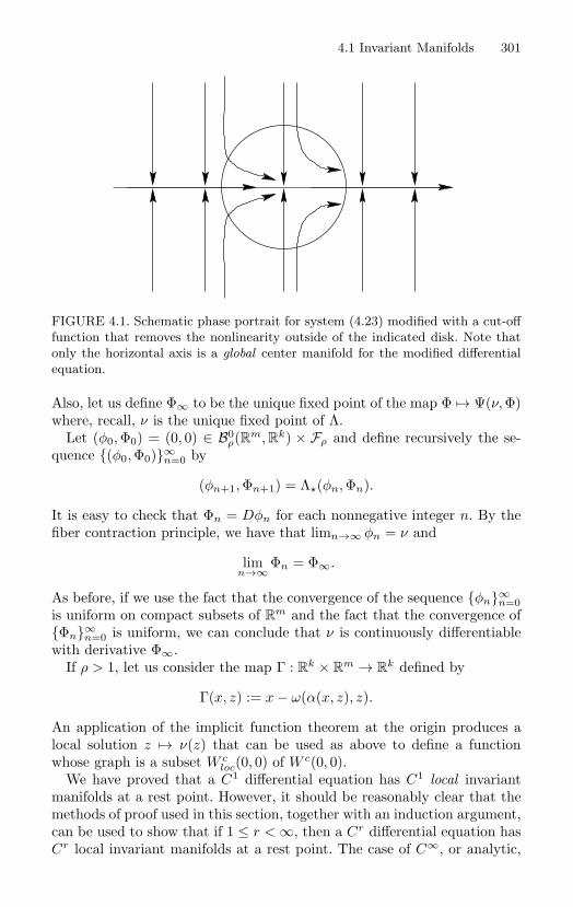
4.1 Invariant Manifolds 301
FIGURE 4.1. Schematic phase portrait for system (4.23) modified with a cut-offfunction that removes the nonlinearity outside of the indicated disk. Note thatonly the horizontal axis is a global center manifold for the modified differentialequation.
Also, let us define Φ∞ to be the unique fixed point of the map Φ → Ψ(ν,Φ)where, recall, ν is the unique fixed point of Λ.
Let (φ0, Φ0) = (0, 0) ∈ B0ρ(Rm, Rk) × Fρ and define recursively the se-
quence (φ0, Φ0)∞n=0 by
(φn+1, Φn+1) = Λ(φn, Φn).
It is easy to check that Φn = Dφn for each nonnegative integer n. By thefiber contraction principle, we have that limn→∞ φn = ν and
limn→∞ Φn = Φ∞.
As before, if we use the fact that the convergence of the sequence φn∞n=0
is uniform on compact subsets of Rm and the fact that the convergence of
Φn∞n=0 is uniform, we can conclude that ν is continuously differentiable
with derivative Φ∞.If ρ > 1, let us consider the map Γ : R
k × Rm → R
k defined by
Γ(x, z) := x − ω(α(x, z), z).
An application of the implicit function theorem at the origin produces alocal solution z → ν(z) that can be used as above to define a functionwhose graph is a subset W c
loc(0, 0) of W c(0, 0).We have proved that a C1 differential equation has C1 local invariant
manifolds at a rest point. However, it should be reasonably clear that themethods of proof used in this section, together with an induction argument,can be used to show that if 1 ≤ r < ∞, then a Cr differential equation hasCr local invariant manifolds at a rest point. The case of C∞, or analytic,
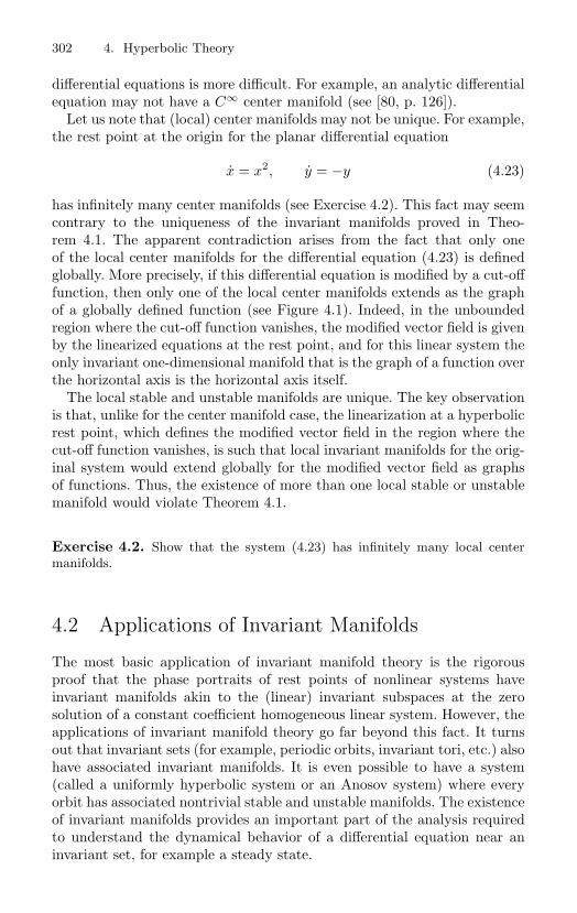
302 4. Hyperbolic Theory
differential equations is more difficult. For example, an analytic differentialequation may not have a C∞ center manifold (see [80, p. 126]).
Let us note that (local) center manifolds may not be unique. For example,the rest point at the origin for the planar differential equation
x = x2, y = −y (4.23)
has infinitely many center manifolds (see Exercise 4.2). This fact may seemcontrary to the uniqueness of the invariant manifolds proved in Theo-rem 4.1. The apparent contradiction arises from the fact that only oneof the local center manifolds for the differential equation (4.23) is definedglobally. More precisely, if this differential equation is modified by a cut-offfunction, then only one of the local center manifolds extends as the graphof a globally defined function (see Figure 4.1). Indeed, in the unboundedregion where the cut-off function vanishes, the modified vector field is givenby the linearized equations at the rest point, and for this linear system theonly invariant one-dimensional manifold that is the graph of a function overthe horizontal axis is the horizontal axis itself.
The local stable and unstable manifolds are unique. The key observationis that, unlike for the center manifold case, the linearization at a hyperbolicrest point, which defines the modified vector field in the region where thecut-off function vanishes, is such that local invariant manifolds for the orig-inal system would extend globally for the modified vector field as graphsof functions. Thus, the existence of more than one local stable or unstablemanifold would violate Theorem 4.1.
Exercise 4.2. Show that the system (4.23) has infinitely many local centermanifolds.
4.2 Applications of Invariant Manifolds
The most basic application of invariant manifold theory is the rigorousproof that the phase portraits of rest points of nonlinear systems haveinvariant manifolds akin to the (linear) invariant subspaces at the zerosolution of a constant coefficient homogeneous linear system. However, theapplications of invariant manifold theory go far beyond this fact. It turnsout that invariant sets (for example, periodic orbits, invariant tori, etc.) alsohave associated invariant manifolds. It is even possible to have a system(called a uniformly hyperbolic system or an Anosov system) where everyorbit has associated nontrivial stable and unstable manifolds. The existenceof invariant manifolds provides an important part of the analysis requiredto understand the dynamical behavior of a differential equation near aninvariant set, for example a steady state.
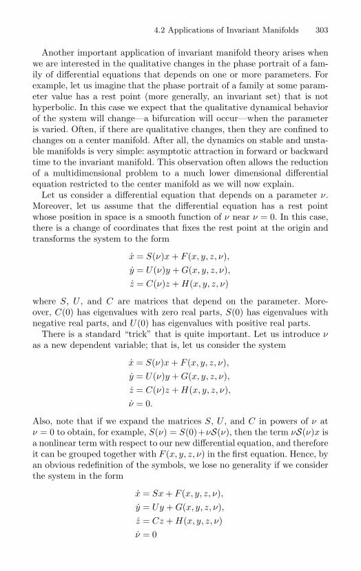
4.2 Applications of Invariant Manifolds 303
Another important application of invariant manifold theory arises whenwe are interested in the qualitative changes in the phase portrait of a fam-ily of differential equations that depends on one or more parameters. Forexample, let us imagine that the phase portrait of a family at some param-eter value has a rest point (more generally, an invariant set) that is nothyperbolic. In this case we expect that the qualitative dynamical behaviorof the system will change—a bifurcation will occur—when the parameteris varied. Often, if there are qualitative changes, then they are confined tochanges on a center manifold. After all, the dynamics on stable and unsta-ble manifolds is very simple: asymptotic attraction in forward or backwardtime to the invariant manifold. This observation often allows the reductionof a multidimensional problem to a much lower dimensional differentialequation restricted to the center manifold as we will now explain.
Let us consider a differential equation that depends on a parameter ν.Moreover, let us assume that the differential equation has a rest pointwhose position in space is a smooth function of ν near ν = 0. In this case,there is a change of coordinates that fixes the rest point at the origin andtransforms the system to the form
x = S(ν)x + F (x, y, z, ν),y = U(ν)y + G(x, y, z, ν),z = C(ν)z + H(x, y, z, ν)
where S, U , and C are matrices that depend on the parameter. More-over, C(0) has eigenvalues with zero real parts, S(0) has eigenvalues withnegative real parts, and U(0) has eigenvalues with positive real parts.
There is a standard “trick” that is quite important. Let us introduce νas a new dependent variable; that is, let us consider the system
x = S(ν)x + F (x, y, z, ν),y = U(ν)y + G(x, y, z, ν),z = C(ν)z + H(x, y, z, ν),ν = 0.
Also, note that if we expand the matrices S, U , and C in powers of ν atν = 0 to obtain, for example, S(ν) = S(0)+νS(ν), then the term νS(ν)x isa nonlinear term with respect to our new differential equation, and thereforeit can be grouped together with F (x, y, z, ν) in the first equation. Hence, byan obvious redefinition of the symbols, we lose no generality if we considerthe system in the form
x = Sx + F (x, y, z, ν),y = Uy + G(x, y, z, ν),z = Cz + H(x, y, z, ν)ν = 0
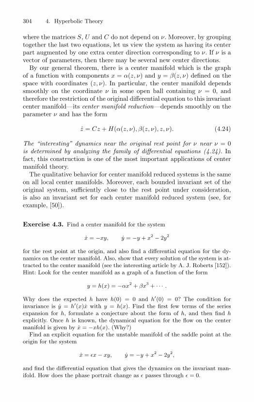
304 4. Hyperbolic Theory
where the matrices S, U and C do not depend on ν. Moreover, by groupingtogether the last two equations, let us view the system as having its centerpart augmented by one extra center direction corresponding to ν. If ν is avector of parameters, then there may be several new center directions.
By our general theorem, there is a center manifold which is the graphof a function with components x = α(z, ν) and y = β(z, ν) defined on thespace with coordinates (z, ν). In particular, the center manifold dependssmoothly on the coordinate ν in some open ball containing ν = 0, andtherefore the restriction of the original differential equation to this invariantcenter manifold—its center manifold reduction—depends smoothly on theparameter ν and has the form
z = Cz + H(α(z, ν), β(z, ν), z, ν). (4.24)
The “interesting” dynamics near the original rest point for ν near ν = 0is determined by analyzing the family of differential equations (4.24). Infact, this construction is one of the most important applications of centermanifold theory.
The qualitative behavior for center manifold reduced systems is the sameon all local center manifolds. Moreover, each bounded invariant set of theoriginal system, sufficiently close to the rest point under consideration,is also an invariant set for each center manifold reduced system (see, forexample, [50]).
Exercise 4.3. Find a center manifold for the system
x = −xy, y = −y + x2 − 2y2
for the rest point at the origin, and also find a differential equation for the dy-namics on the center manifold. Also, show that every solution of the system is at-tracted to the center manifold (see the interesting article by A. J. Roberts [152]).Hint: Look for the center manifold as a graph of a function of the form
y = h(x) = −αx2 + βx3 + · · · .
Why does the expected h have h(0) = 0 and h′(0) = 0? The condition forinvariance is y = h′(x)x with y = h(x). Find the first few terms of the seriesexpansion for h, formulate a conjecture about the form of h, and then find hexplicitly. Once h is known, the dynamical equation for the flow on the centermanifold is given by x = −xh(x). (Why?)
Find an explicit equation for the unstable manifold of the saddle point at theorigin for the system
x = εx − xy, y = −y + x2 − 2y2,
and find the differential equation that gives the dynamics on the invariant man-ifold. How does the phase portrait change as ε passes through ε = 0.
4.3 The Hartman–Grobman Theorem 305
Exercise 4.4. Find the third order Taylor series approximation of the (scalar)center manifold reduced family at the origin, as in display (4.24), for the system
z = ε − z + w +14((1 + ε)z2 − 2εwz − (1 − ε)w2),
w = ε + z − w − 14((1 + ε)z2 − (2ε − 4)wz + (3 + ε)w2).
4.3 The Hartman–Grobman Theorem
In the last section we proved the existence of stable and unstable manifoldsfor hyperbolic rest points of differential equations using a classic idea thatis worth repeating: The existence of the desired object, for example aninvariant manifold, is equivalent to the existence of a fixed point for aproperly defined map on a function space, and the hyperbolicity hypothesisis used to prove that this map is a contraction. This same idea is used in thissection to prove the Hartman–Grobman theorem (Theorem 1.27). See [9],[126], [144], [139], and [150] for the origins of this marvelous proof, and forthe original proofs see [79] and [87].
4.3.1 DiffeomorphismsLet us consider the Hartman–Grobman theorem for a discrete dynamicalsystem, that is, a dynamical system defined by a diffeomorphism F : R
n →R
n as follows: If ξ ∈ Rn, then the orbit of ξ is the set of all iterates
of ξ under transformation by F . More precisely, if we use the notationF−1 for the inverse of F , define F 0(ξ) = ξ and use the inductive identityF +1(ξ) := F (F (ξ)) to define F for every integer , then the orbit of ξis the set F (ξ) : ∈ Z. A fixed point of the dynamical system definedby F is analogous to a rest point for the dynamical system defined by adifferential equation.
There is, of course, a very close connection between the dynamical sys-tems defined by differential equations and those defined by diffeomor-phisms. If, for example, ϕt is the flow of an autonomous differential equa-tion, then for each fixed t ∈ R the time t map given by ξ → ϕt(ξ) isa diffeomorphism on its domain that defines a dynamical system whoseorbits are all subsets of the orbits of the flow. Also, a Poincare map is adiffeomorphism whose orbits correspond to features of the phase portrait ofits associated differential equation. In particular, a fixed point of a Poincaremap corresponds to a periodic orbit of the associated differential equation.
If ϕt is the flow for the differential equation x = f(x), then recall thatt → Dφt(ζ) is the solution of the variational initial value problem
W = Df(ϕt(ζ))W, W (0) = I.
306 4. Hyperbolic Theory
In particular, if ζ is a rest point, then the solution of the initial valueproblem is
Dφt(ζ) = etDf(ζ).
Thus, if ζ is a hyperbolic rest point and t = 0, then the linear transfor-mation Dφt(ζ) has no eigenvalues on the unit circle of the complex plane.For this reason, a fixed point of a diffeomorphism is called hyperbolic if thederivative of the diffeomorphism at the fixed point has no eigenvalue onthe unit circle.
The next theorem is a version of the Hartman–Grobman theorem fordiffeomorphisms. Informally, it states that the phase portrait near a hy-perbolic fixed point is the same, up to a continuous change of coordinates,as the phase portrait of the dynamical system induced by the derivative ofthe diffeomorphism evaluated at the fixed point.
Theorem 4.5 (Hartman–Grobman). If ζ is a hyperbolic fixed point forthe diffeomorphism F : R
n → Rn, then there is an open set U ∈ R
n
containing ζ and a homeomorphism H with domain U such that
F (H(x)) = H(DF (ζ)x)
whenever x ∈ U and both sides of the equation are defined.
The proof of Theorem 4.5 is based on the idea that the conjugating homeo-morphism is the solution of a functional equation. Sufficient conditions forthe appropriate functional equation to have a unique solution are given inthe following key lemma.
Lemma 4.6. Suppose that A : Rn → R
n is an invertible hyperbolic lineartransformation and p : R
n → Rn is a smooth function. If 0 < α < 1 and
the C1-norm of the function p is sufficiently small, then there is a uniquecontinuous function h : R
n → Rn such that ‖h‖ ≤ α, h(0) = 0, and
h(Ax) − Ah(x) = p(x + h(x)) (4.25)
for every x in Rn.
Proof. For h : Rn → R
n, define the linear operator L by
L(h)(x) = h(Ax) − Ah(x),
the (nonlinear) operator Φ by
Φ(h)(x) = p(x + h(x)) − p(x),
and recast equation (4.25) in the form
L(h)(x) = Φ(h)(x) + p(x). (4.26)
4.3 The Hartman–Grobman Theorem 307
The operator L is invertible on the Banach space C(Rn), the space ofbounded continuous transformations of R
n with the supremum norm. Toprove this fact, let us use the hyperbolicity of the linear transformationA to decompose the space R
n as the direct sum of the invariant lineareigenspaces Es and Eu that correspond, respectively, to the subsets of thespectrum of A that lie inside and outside of the unit circle. Of course, ifthe fixed point is a sink or a source, then there is only one eigenspace.
By Corollary 2.85, there are adapted norms (both denoted by | |) on theeigenspaces such that the sum of these norms is equivalent to the normon R
n, and in addition there is a number λ, with 0 < λ < 1, such that ifx = xs + xu ∈ Es ⊕ Eu, then
|Axs| < λ|xs|, |A−1xu| < λ|xu|.
Also, if h is a transformation of Rn, then h can be expressed uniquely as a
sum of functions h = hs + hu where hs : Rn → Es and hu : R
n → Eu.Using the projections to Es and Eu, let us note that
L(h)(x) = [hs(Ax) − A(hs(x))] + [hu(Ax) − A(hu(x))].
Because the eigenspaces are invariant sets for A, it follows the equation
L(h)(x) = p(x),
where p : Rn → R
n, has a solution h if and only if the “operator equations”
Ls(hs)(x) := hs(Ax) − Ahs(x) = ps(x),
Lu(hu)(x) := hu(Ax) − Ahu(x) = pu(x)
both have solutions. In particular, to prove that L is invertible, it sufficesto prove that Ls and Lu are both invertible as operators on the respec-tive spaces C0(Rn, Es) and C0(Rn, Eu) where C0(Rn, Es), respectivelyC0(Rn, Eu), denotes the space of continuous bounded functions from R
n
to Es, respectively Eu, with the adapted norm.Let us define two additional operators S and U by
S(hs)(x) := hs(Ax), U(hu)(x) := hu(Ax)
so that
Ls(hs) = (S − A)hs, Lu(hu) = (U − A)hu.
Because A is invertible, both of the operators S and U are invertible; forexample, we have that S−1(hs)(x) = hs(A−1x). Moreover, it is easy toprove directly from the definition of the operator norm that these operatorsand their inverses all have norm one. It follows that
‖S−1A‖ ≤ ‖S−1‖ ‖A‖ < λ < 1,
308 4. Hyperbolic Theory
and therefore the operator I − S−1A is invertible. In fact, its inverse isgiven by
I − S−1A = I +∞∑
=1
(S−1A)
where the Neumann series is easily proved to be absolutely convergent bycomparison with the geometric series
∞∑=0
λ =1
1 − λ.
Because the operator Ls can be rewritten in the form
Ls = S − A = S(I − S−1A),
it is invertible with inverse
L−1s = (I − S−1A)−1S−1.
Moreover, we have the following norm estimate:
‖L−1s ‖ ≤ 1
1 − λ.
Similarly, for the operator Lu, we have that
Lu = U − A = A(A−1U − I) = −A(I − A−1U)
with
‖A−1U‖ < λ < 1.
Therefore, the inverse of Lu is given by
L−1u = −(I − A−1U)−1A−1,
and, in addition, we have the norm estimate
‖L−1u ‖ ≤ λ
1 − λ<
11 − λ
.
Using the fact that both Ls and Lu are invertible and using the normestimates for their inverses, it follows that L is invertible and
‖L−1‖ <2
1 − λ.
Let us recast equation (4.26) in the form
h = L−1Φ(h) + L−1p
4.3 The Hartman–Grobman Theorem 309
and note that the solutions of equation (4.26) are exactly the fixed pointsof the operator T defined by
T (h) := L−1Φ(h) + L−1p.
Also, the set
C0α := h ∈ C0(Rn) : ‖h‖ ≤ α, h(0) = 0
is a complete metric subspace of the Banach space C0(Rn). Thus, to com-plete the proof of the lemma, it suffices to show the following proposition:T : C0
α → C0α and T is a contraction.
To prove the proposition, note that if h(0) = 0, then T (h)(0) = 0, andalso that
‖T (h)‖ ≤ ‖L−1‖(‖Φ(h)‖ + ‖p‖)
≤ 11 − λ
(sup
x∈Rn
|p(x + h(x)) − p(x)| + ‖p‖)
≤ 11 − λ
(sup
x∈Rn
|Dp(x)| ‖h‖ + ‖p‖)
≤ 11 − λ
(‖p‖1‖h‖ + ‖p‖
)≤ 1
1 − λ(1 + α)‖p‖1
where ‖ ‖1 denotes the C1 norm. Hence, if
‖p‖1 <α
1 + α(1 − λ),
then T is a transformation of the space C0α. Moreover, because
‖T (h1) − T (h2)‖ = ‖L−1(Φ(h1) − Φ(h2))‖
≤ 11 − λ
supx∈Rn
‖p(x + h1(x)) − p(x + h2(x))‖
≤ 11 − λ
‖p‖1‖h1 − h2‖,
the same restriction on the size of ‖p‖1 ensures that T is a contraction.
Let us prove Theorem 4.5.
Proof. Assume, without loss of generality, that ζ is the origin of Rn. Also,
define A := DF (0) and note that, because F is a diffeomorphism, A is aninvertible hyperbolic linear transformation.
Choose α ∈ R such that 0 < α < 1. If we define f(x) := F (x)−Ax, thenf(0) = 0 and Df(0) = 0. Thus, using the continuity of f , there is an open
310 4. Hyperbolic Theory
neighborhood V of the origin such that the C1-norm of the restriction of fto V is less than α/3. This norm is defined as usual in terms of C0-normsas follows
‖f‖1 = ‖f‖ + ‖Df‖.
By using an appropriate bump function, as in the derivation of the esti-mate (4.21), there is a smooth function f∗ defined on all of R
n such thatf = f∗ on V and the C1-norm of f∗ (with the supremum taken over R
n)does not exceed three times the C1-norm of the restriction of f to V ; thatis, since ‖f‖1 ≤ α/3, we have that ‖f∗‖1 < α.
Apply Lemma 4.6 with p = f∗ and define a new continuous functionH : R
n → Rn by
H(x) = x + h(x). (4.27)
Using equation (4.25), it is easy to see that F (H(x)) = H(A(x)) for allx ∈ R
n. This function H, restricted to a suitably small neighborhood ofthe origin, is a candidate for the required local homeomorphism. Indeed,to complete the proof of the theorem, we will show that there is an openset U containing the origin and contained in V such that the restriction ofH to U is a homeomorphism.
To prove that H is injective, let us suppose that H(x) = H(y) for somepoints x and y in R
n. Using the identities
H(Ax) = F (H(x)) = F (H(y)) = H(Ay),
we have that
H(Ax) = H(Ay)
for every integer . But then
Ax + h(Ax) = Ay + h(Ay)
and
‖Ax − Ay‖ = ‖h(Ax) − h(Ay)‖ ≤ 2‖h‖.
In particular, the set
‖A(x − y)‖ : ∈ Z
is bounded. But this is a contradiction unless x = y. In fact, because A isa hyperbolic linear transformation on R
n, if z = 0, then either
lim→∞
‖Az‖ = ∞, or lim→−∞
‖Az‖ = ∞.
4.3 The Hartman–Grobman Theorem 311
Thus, H is injective.There is an open neighborhood U of the origin such that its closure U
is compact, contained in V , and H(U) ⊂ V . Because H is a continuousinjective function on the compact set U ⊂ R
n, an elementary argumentusing point set topology [129, p. 167] shows that H restricted to U is ahomeomorphism onto its image. In particular, H has a continuous inversedefined on H(U). This inverse restricted to H(U) is still continuous. Thus,H restricted to U is a homeomorphism onto its image.
4.3.2 Differential EquationsIn this section we will prove the following version of the Hartman–Grobmantheorem for a hyperbolic rest point of an autonomous differential equation.
Theorem 4.7. Suppose that ζ is a rest point of the differential equationx = f(x) on R
n with flow ϕt and ψt is the flow of the linearized systemx = Df(ζ)(x − ζ). If ζ is a hyperbolic rest point, then there is an opensubset U of R
n such that ζ ∈ U and a homeomorphism G with domainU such that G(ϕt(x)) = ψt(G(x)) whenever x ∈ U and both sides of theequation are defined.
While the proofs of Theorem 4.7 and the Hartman–Grobman theorem fordiffeomorphisms are similar, there are some subtle differences. For example,note that whereas the conjugating homeomorphism H in the diffeomor-phism case is a solution of the functional equation F (G(x)) = G(DF (ζ)x),the corresponding equation in Theorem 4.7 has the form
G(F (x)) = DF (ζ)G(x).
If G is a homeomorphism, then these two equations are equivalent. But,the form of these equations is important for the method used here to provethe existence of G.
Let us begin with a lemma analogous to Lemma 4.6. For the statementof this lemma, recall that C(Rn) denotes the Banach space of boundedcontinuous transformations of R
n with the supremum norm.
Lemma 4.8. If A : Rn → R
n is an invertible hyperbolic linear transfor-mation and F : R
n → Rn is a homeomorphism, then the operator given
by
Φ(g)(x) = Ag(x) − g(F (x))
is a bounded linear transformation with a bounded inverse on the Banachspace C(Rn).
Proof. If g ∈ C(Rn), then clearly x → Φ(g)(x) is a continuous trans-formation of R
n. Also, it is clear that Φ is a linear operator. The norm
312 4. Hyperbolic Theory
estimate
|Φ(g)(x)| ≤ |Ag(x)| + |g(F (x))| ≤ ‖A‖ ‖g‖ + ‖g‖
(where ‖A‖ is the operator norm of the linear transformation A and ‖g‖ isthe supremum norm of the function g), shows that Φ is a bounded linearoperator on C(Rn).
The proof that the operator Φ has a bounded inverse is similar to theproof of Lemma 4.6. In fact, relative to the splitting R
n = Es ⊕ Eu, theoperator Φ is given by Φ = Φs + Φu where
Φs(gs) := A gs − gs F, Φu(gu) := A gu − gu F.
The important point is that the operators S and U defined by
S(gs) := gs F, U(gu) := gu F
and their inverses are all bounded, and they all have operator norm one.The operators Φs and Φu are inverted using Neumann series, as in theproof of Lemma 4.6.
Let us prove Theorem 4.7.
Proof. Assume that ζ = 0 and define B := Df(0). Also, note that
ψt(x) = etBx
and define A := ψ1, the time-one map of the flow ψt.By using an appropriate bump function γ defined on a neighborhood of
the origin, the differential equation
x = f∗(x), (4.28)
where f∗ := γf , has a complete flow ϕ∗t together with the following addi-
tional properties.(i) The function f∗ : R
n → Rn has a finite Lipschitz constant.
(ii) There is an open neighborhood V of the origin such that the timeone map F := ϕ∗
1 agrees with the time one map ϕ1 of the flow ϕ1on V .
(iii) The function p(x) := F (x) − Ax has finite C1-norm that is suffi-ciently small so that, by Lemma 4.6, there is a function h ∈ C(Rn)with h(0) = 0, ‖h‖ < 1, and
h(Ax) − Ah(x) = p(x + h(x))
for all x ∈ Rn.
4.3 The Hartman–Grobman Theorem 313
Let us prove first that there is a continuous map G : Rn → R
n such thatG(F (x)) = A(G(x); that is, G conjugates the time one maps of the linearand nonlinear flows. In fact, because p has finite C1-norm, it follows thatp ∈ C(Rn) and by Lemma 4.8, there is a unique g ∈ C(Rn) such that
Ag(x) − g(F (x)) = p(x).
Thus, if we define G by G(x) = x + g(x), then we have that
G(F (x)) = AG(x). (4.29)
To construct a conjugacy between the linear and the nonlinear flows, usethe “time one conjugacy” G to define G : R
n → Rn by
G(x) :=∫ 1
0ψ−s(G(ϕ∗
s(x))) ds.
We will show that
ψt(G(x)) = G(ϕ∗t (x)). (4.30)
In fact, using the linearity of ψt, the change of variables τ = s + t − 1, theflow property, and equation (4.29), we have
ψt(G(ϕ∗t (x))) =
∫ 1
0ψ−t−s(G(ϕ∗
s+t(x))) ds
=∫ t
t−1ψ−τ (ψ−1(G(ϕ∗
1(ϕ∗τ (x))) dτ
=∫ t
t−1ψ−τ (G(ϕ∗
τ (x))) dτ.
If we split the last integral into the two parts∫ 0
t−1ψ−τ (G(ϕ∗
τ (x))) dτ +∫ t
0ψ−τ (G(ϕ∗
τ (x))) dτ,
change variables by σ := τ+1 in the first integral, and use the flow propertytogether with equation (4.29), then we obtain the identity
ψt(G(ϕ∗t (x))) =
∫ 1
t
ψ−σ+1(G(ϕ∗−1+σ(x))) dσ +
∫ t
0ψ−τ (G(ϕ∗
τ (x))) dτ
= G(x),
as required.Recall equation (4.29) and note that if we set t = 1 in equation (4.30),
then we have the functional identities
G(F (x)) = AG(x), G(F (x)) = AG(x).
314 4. Hyperbolic Theory
By Lemma 4.8, the function G is unique among all continuous transforma-tions of R
n of the form G(x) = x + g(x) that satisfy the same functionalequation, provided that g ∈ C(Rn). Thus, to prove that G = G, it sufficesto show that the function x → G(x) − x is in C(Rn). To see this fact, letus note first that we have the identities
G(x) − x =∫ 1
0ψ−s(G(ϕ∗
s(x))) ds − x
=∫ 1
0ψ−s[G(ϕ∗
s(x)) − ψt(x)] ds
=∫ 1
0ψ−s[G(ϕ∗
s(x)) − ϕ∗s(x) + ϕ∗
s(x) − ψt(x)] ds,
and the estimate
|G(x) − x| ≤ e‖B‖( |G(ϕ∗s(x)) − ϕ∗
s(x)| + |ϕ∗s(x) − ψt(x)| )
≤ e‖B‖( ‖g‖ + sup0≤s≤1
|ϕ∗s(x) − ψs(x)| ).
Also, for 0 ≤ s ≤ 1, we have the inequalities
|ϕ∗s(x) − ψs(x)| ≤
∫ s
0|f∗(ϕ∗
t (x)) − Bφt(x)| dt
≤∫ s
0|f∗(ϕ∗
t (x)) − f∗(ψt(x))| + |f∗(ψt(x)) − Bφt(x)| dt
≤∫ s
0Lip(f∗)|ϕ∗
t (x) − ψt(x)| dt + (‖f∗‖ + ‖B‖e‖B‖).
Thus, by Gronwall’s inequality,
sup0≤s≤1
|ϕ∗s(x) − ψs(x)| ≤ (‖f∗‖ + ‖B‖e‖B‖)eLip(f∗),
and, as a result, the function x → G(x) − x is in C(Rn).It remains to show that G = G is a homeomorphism when restricted to
some neighborhood of the origin. Using property (iii) given above and theproof of the Hartman–Grobman theorem for diffeomorphisms, the functionh given in property (iii) can be use to define a continuous function H byH(x) = x + h(x) so that
F (H(x)) = H(Ax).
Thus,
G(H(Ax)) = G(F (H(x))) = AG(H(x))
4.3 The Hartman–Grobman Theorem 315
and, with K := GH, we have K(A(x)) = A(K(x)). Moreover, the functionK has the form
K(x) = x + h(x) + g(x + h(x))
where, by the construction of G and H, the function
α : x → +h(x) + g(x + h(x))
is in C(Rn) and A(α(x)) − α(Ax) = 0. By Lemma 4.8, there is only onefunction α in C(Rn) that solves this functional equation. It follows thatα(x) ≡ 0. Therefore, K is the identity function and G(H(x)) = x for allx ∈ R
n. Because there is an open set U containing the origin such that therestriction of H to U is a homeomorphism onto its image, we must havethat G restricted to H(U) is the inverse of H. In particular, G restrictedto H(U) is a homeomorphism onto U .
Exercise 4.9. Suppose A is an invertible linear transformation of Rn. Let L
denote the set of all Lipschitz functions mapping Rn to R
n and, for α ∈ L, letLip(α) denote the (least) Lipschitz constant for α. Prove: There is an ε > 0 suchthat if α ∈ L and Lip(α) < ε, then A + α : R
n → Rn is continuous and bijective.
Exercise 4.10. [Toral Automorphisms] Consider the torus T2 = R
2/Z2, that
is, all equivalence classes of points in the plane where two points are equivalentif their difference is in the integer lattice. A unimodular matrix, for example
A :=(
2 11 1
),
induces a map on T2 called a toral automorphism. Prove that A is a hyperbolic
linear map (spectrum off the unit circle). Prove that the induced map on T2
is invertible. Determine all periodic points of the induced map. Prove that theinduced map has a dense orbit. Show that every orbit of the induced map has aone-dimensional stable and a one-dimensional unstable manifold, the sets definedas the points in T
2 that are asymptotic to the given orbit under forward, respec-tively backward, iteration. Hyperbolic toral automorphisms are the prototypicalexamples of Anosov (uniformly hyperbolic) dynamical systems and they enjoymany interesting dynamical properties; for example, they are “chaotic maps”where the entire phase space is a “chaotic attractor”. Also, note that toral auto-morphisms are examples of area preserving dynamical systems: the measures ofsubsets of the phase space do not change under iteration by the map. (The flowof a Hamiltonian system has the same property.) The hyperbolic toral automor-phisms are ergodic; that is, they are area preserving maps such that every one oftheir invariant sets has measure zero or measure one. Hint: See [100]. The firstorder system x = 1, y = α induces a flow on the torus (where x and y are viewedas angular variables modulo one). Prove that its flow is measure preserving. Provethat the flow is ergodic if α is irrational.
5Continuation of Periodic Solutions
A fundamental engineering problem is to determine the response of a phys-ical system to an applied force. In this chapter some mathematical ideasare introduced that can be used to address a classic case of this problemwhere the physical system is an oscillator that is modeled by a differentialequation with periodic orbits and the applied force is modeled as a “small”perturbation. Partial answers to several important questions will be given.Which, if any, of the unperturbed periodic orbits persist under the per-turbation? Are the perturbed periodic orbits stable? Can the perturbedperiodic orbits be approximated by analytic formulas? We will restrict ourdiscussion to planar systems, the case of most practical value. However,many of the results of this chapter can be easily generalized to multidi-mensional systems.
The subject of this chapter has a long history in applied science andmathematics; it is still an active area of mathematical research. Thus,there is a mathematical and scientific literature on this subject that is fartoo extensive to be reviewed here. However, every student of the subjectshould be aware of the classic books by Aleksandr A. Andronov, AleksandrA. Vitt, and Semen E. Khaiken [7], Nikolai N. Bogoliubov and Yuri A.Mitropolsky [23], Chihiro Hayashi [89], Nikolai Minorsky [125], and JamesJ. Stoker [169]; and the more recent works of Miklos Farkas [63], John Guck-enheimer and Philip Holmes [80], Jack K. Hale [83], Jirair K. Kevorkianand Julian D. Cole [101], James Murdock [130], Ali H. Nayfey [133], andStephen W. Wiggins [185].
318 5. Continuation of Periodic Solutions
5.1 A Classic Example: van der Pol’s Oscillator
An important mathematical model in the history of our subject is knownas van der Pol’s equation
x + ε(x2 − 1)x + ω2x = a sin Ωt. (5.1)
This differential equation was introduced by Lord Rayleigh [146] in 1883.Balthasar van der Pol [176] investigated it more extensively when he studiedthe equation in 1926 as a model of the voltage in a triode circuit. How-ever, since its introduction, this differential equation has been suggestedas a model for many different physical phenomena. For example, just twoyears after van der Pol’s initial paper, van der Pol and Johannes van derMark [178] proposed the equation as a model for the human heartbeat. Wewill use the differential equation (5.1) to illustrate some of the ideas thatwill be explored more fully later in this chapter.
Let us observe some of the dynamical features of the van der Pol equa-tion. If a = 0 and ε = 0, then equation (5.1) is the familiar model of a linearspring; that is, a spring with restoring force modeled by Hooke’s law. Thisequation is often referred to as the spring equation or the harmonic oscilla-tor. The term a sin Ωt represents a periodic external force with amplitude a,period 2π/Ω and frequency Ω. The term ε(x2 −1)x can be viewed as repre-senting a nonlinear damping. The “direction” of this damping depends onthe state (x, x) of the system where x represents position and x representsvelocity. In fact, the energy of the spring is given by
E :=12x2 +
12ω2x2,
and has time derivative
E = ax sin Ωt − ε(x2 − 1)x2.
Thus, energy due to the damping leaves the system while |x| > 1 and isabsorbed while |x| < 1.
Our subject is motivated by the following basic question: If the currentstate of the system is known, what does the model predict about its futurestates? Even though the van der Pol equation has been studied intensively,we cannot give a complete answer to this question. However, as we will see,many useful predictions can be made. In particular, in this section we willshow how to determine the steady state behavior of the system when thereis no external force and the damping is small.
Let us consider the unforced, weakly damped, scaled van der Pol equationgiven by
x + ε(x2 − 1)x + x = 0. (5.2)
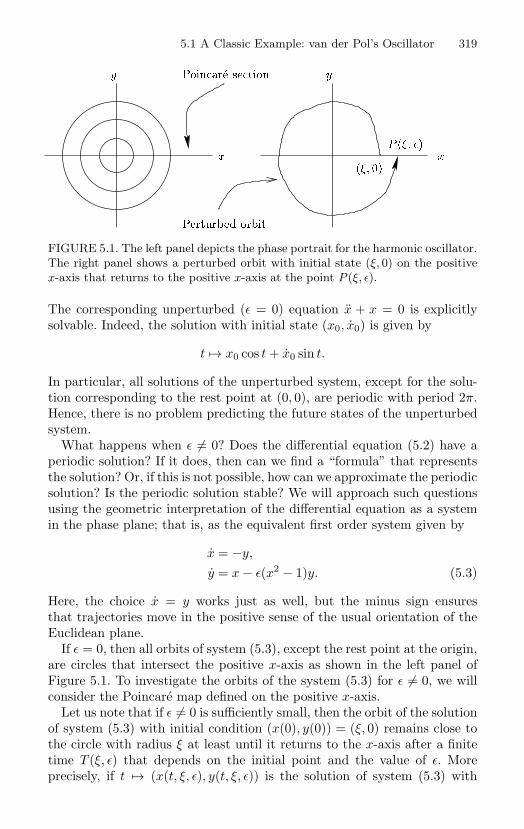
5.1 A Classic Example: van der Pol’s Oscillator 319
yy
x
Perturbed orbit
Poincare section
P
x
FIGURE 5.1. The left panel depicts the phase portrait for the harmonic oscillator.The right panel shows a perturbed orbit with initial state (ξ, 0) on the positivex-axis that returns to the positive x-axis at the point P (ξ, ε).
The corresponding unperturbed (ε = 0) equation x + x = 0 is explicitlysolvable. Indeed, the solution with initial state (x0, x0) is given by
t → x0 cos t + x0 sin t.
In particular, all solutions of the unperturbed system, except for the solu-tion corresponding to the rest point at (0, 0), are periodic with period 2π.Hence, there is no problem predicting the future states of the unperturbedsystem.
What happens when ε = 0? Does the differential equation (5.2) have aperiodic solution? If it does, then can we find a “formula” that representsthe solution? Or, if this is not possible, how can we approximate the periodicsolution? Is the periodic solution stable? We will approach such questionsusing the geometric interpretation of the differential equation as a systemin the phase plane; that is, as the equivalent first order system given by
x = −y,
y = x − ε(x2 − 1)y. (5.3)
Here, the choice x = y works just as well, but the minus sign ensuresthat trajectories move in the positive sense of the usual orientation of theEuclidean plane.
If ε = 0, then all orbits of system (5.3), except the rest point at the origin,are circles that intersect the positive x-axis as shown in the left panel ofFigure 5.1. To investigate the orbits of the system (5.3) for ε = 0, we willconsider the Poincare map defined on the positive x-axis.
Let us note that if ε = 0 is sufficiently small, then the orbit of the solutionof system (5.3) with initial condition (x(0), y(0)) = (ξ, 0) remains close tothe circle with radius ξ at least until it returns to the x-axis after a finitetime T (ξ, ε) that depends on the initial point and the value of ε. Moreprecisely, if t → (x(t, ξ, ε), y(t, ξ, ε)) is the solution of system (5.3) with
320 5. Continuation of Periodic Solutions
initial condition
x(0, ξ, ε) = ξ, y(0, ξ, ε) = 0,
then, as long as ε is sufficiently small, the trajectory of this solution willreturn to the positive x-axis at the point with coordinate x(T (ξ, ε), ξ, ε).The function (ξ, ε) → P (ξ, ε) given by
P (ξ, ε) := x(T (ξ, ε), ξ, ε) (5.4)
is called the parametrized return map (see the right panel of Figure 5.1).If P (ξ, ε) = ξ, then t → (x(t, ξ, ε), y(t, ξ, ε)) is a periodic solution of the
system (5.3) with period T (ξ, ε). In other words, if ξ is a fixed point ofthe map ξ → P (ξ, ε) or a zero of the associated displacement functionδ(ξ, ε) = x(T (ξ, ε), ξ, ε) − ξ, then (ξ, 0) is the initial point for a periodicorbit of the perturbed system.
Because δ(ξ, 0) ≡ 0, it is natural to look for the root ξ implicitly as afunction β of ε such that, for ε = 0, the point ξ = β(ε) is the initial pointof a periodic solution of system (5.3). More precisely, we seek a function βdefined on some neighborhood of ε = 0 in R such that δ(β(ε), ε) ≡ 0. Theobvious way to find an implicit solution is to apply the implicit functiontheorem (Theorem 1.182).
In the present context, the displacement function is defined by δ : U ×V → R where U and V are both open subsets of R. Moreover, we havethat δ(ξ, 0) ≡ 0. If there were some point (ξ, 0) such that δξ(ξ, 0) = 0, thenby the implicit function theorem there would be an implicit solution andour problem would be solved. But it is clear that the hypothesis of theimplicit function theorem is not satisfied. In fact, because δ(ξ, 0) ≡ 0, wehave that δξ(ξ, 0) ≡ 0. However, the implicit function theorem does applyafter a further reduction.
Let us use the Taylor series of δ at ε = 0 to obtain the equation
δ(ξ, ε) = εδε(ξ, 0) + O(ε2)
where the O(ε2) term denotes the remainder. This notation is used formallyin the following way: The statement f(ε) = g(ε) + O(ε2) means that thereare constants K > 0 and ε0 > 0 such that the inequality
|f(ε) − g(ε)| < Kε2.
holds for |ε| < ε0. The required reduction is accomplished by defining anew function
∆(ξ, ε) := δε(ξ, 0) + O(ε)
so thatδ(ξ, ε) = ε(δε(ξ, 0) + O(ε)) = ε∆(ξ, ε).
5.1 A Classic Example: van der Pol’s Oscillator 321
Clearly, if there is a function ε → β(ε) such that ∆(β(ε), ε) ≡ 0, thenδ(β(ε), ε) ≡ 0.
Even though the implicit function theorem does not apply to the dis-placement function δ, it might well apply to the function ∆. At any rate,we have reduced the original search for a periodic solution of the per-turbed van der Pol equation to the problem of finding implicit solutionsof the equation ∆(ξ, ε) = 0. Thus, by the implicit function theorem, wehave the following proposition: If ξ > 0 is a simple zero of the functionξ → ∆(ξ, 0), that is, ∆(ξ, 0) = 0 and ∆ξ(ξ, 0) = 0, or equivalently ifδε(ξ, 0) = 0 and δξε(ξ, 0) = 0, then an implicit solution ξ = β(ε) exists. Thefunction ξ → δε(ξ, 0) is called the reduced displacement function, and a sim-ple zero of the reduced bifurcation function (respectively the correspondingunperturbed periodic orbit) is called a continuation point of periodic solu-tions of the system (5.3) (respectively a continuable periodic orbit). Also, aperiodic orbit is said to persist if it is continuable. The ideas used to proveour proposition recur in every continuation problem that we will consider;their implementation constitutes the first part, called the reduction step,in the solution of the continuation problem.
The second part of the continuation method is the identification step,that is, the identification of the reduced displacement function in termsof the original differential equation. For system (5.3), perhaps the mostdirect route to the identification of the reduced displacement function isvia a change to polar coordinates. However, as an illustration of a generalmethod, let us work directly in the original variables and identify the re-duced function by solving a variational equation derived from system (5.3).
To carry out the identification step, apply the chain rule to compute thepartial derivative
δε(ξ, 0) = x(T (ξ, 0), ξ, 0)Tε(ξ, 0) + xε(T (ξ, 0), ξ, 0)
and evaluate at ε = 0 to obtain the equality
x(T (ξ, 0), ξ, 0) = −y(0, ξ, 0) = 0.
In particular, the function ξ → x(T (ξ, 0), ξ, 0)Tε(ξ, 0) and all of its deriva-tives vanish. Thus, to complete the identification step it suffices to deter-mine the partial derivative xε(T (ξ, 0), ξ, 0). To do this, let us compute thepartial derivative with respect to ε at ε = 0 of both sides of the differen-tial equation (5.3) to obtain a variational equation. Also, let us computethe partial derivative with respect to ε of both sides of each of the ini-tial conditions x(0, ξ, ε) = ξ and y(0, ξ, ε) = 0 to obtain the corresponding(variational) initial value problem
xε = −yε, yε = xε − (x2 − 1)y, xε(0, ξ, 0) = 0, yε(0, ξ, 0) = 0 (5.5)
whose solution is t → (xε(t, ξ, 0), yε(t, ξ, 0)).
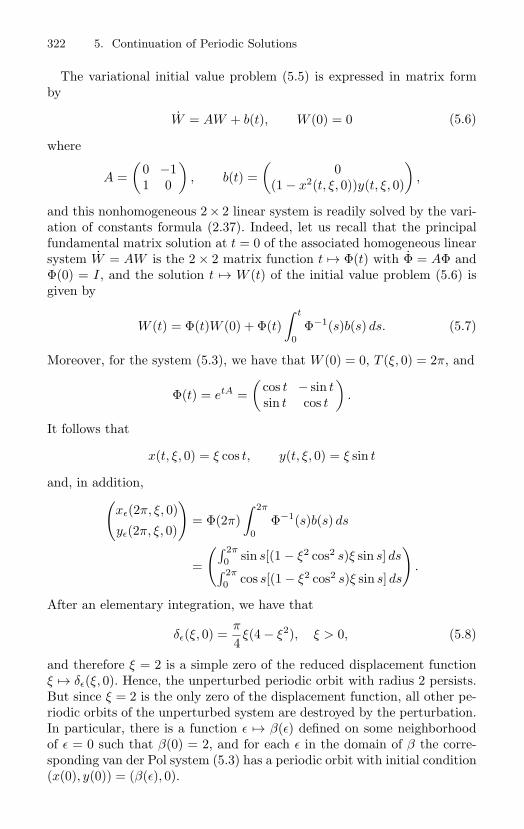
322 5. Continuation of Periodic Solutions
The variational initial value problem (5.5) is expressed in matrix formby
W = AW + b(t), W (0) = 0 (5.6)
where
A =(
0 −11 0
), b(t) =
(0
(1 − x2(t, ξ, 0))y(t, ξ, 0)
),
and this nonhomogeneous 2 × 2 linear system is readily solved by the vari-ation of constants formula (2.37). Indeed, let us recall that the principalfundamental matrix solution at t = 0 of the associated homogeneous linearsystem W = AW is the 2 × 2 matrix function t → Φ(t) with Φ = AΦ andΦ(0) = I, and the solution t → W (t) of the initial value problem (5.6) isgiven by
W (t) = Φ(t)W (0) + Φ(t)∫ t
0Φ−1(s)b(s) ds. (5.7)
Moreover, for the system (5.3), we have that W (0) = 0, T (ξ, 0) = 2π, and
Φ(t) = etA =(
cos t − sin tsin t cos t
).
It follows that
x(t, ξ, 0) = ξ cos t, y(t, ξ, 0) = ξ sin t
and, in addition,(xε(2π, ξ, 0)
yε(2π, ξ, 0)
)= Φ(2π)
∫ 2π
0Φ−1(s)b(s) ds
=
(∫ 2π
0 sin s[(1 − ξ2 cos2 s)ξ sin s] ds∫ 2π
0 cos s[(1 − ξ2 cos2 s)ξ sin s] ds
).
After an elementary integration, we have that
δε(ξ, 0) =π
4ξ(4 − ξ2), ξ > 0, (5.8)
and therefore ξ = 2 is a simple zero of the reduced displacement functionξ → δε(ξ, 0). Hence, the unperturbed periodic orbit with radius 2 persists.But since ξ = 2 is the only zero of the displacement function, all other pe-riodic orbits of the unperturbed system are destroyed by the perturbation.In particular, there is a function ε → β(ε) defined on some neighborhoodof ε = 0 such that β(0) = 2, and for each ε in the domain of β the corre-sponding van der Pol system (5.3) has a periodic orbit with initial condition(x(0), y(0)) = (β(ε), 0).
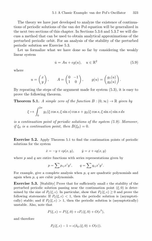
5.1 A Classic Example: van der Pol’s Oscillator 323
The theory we have just developed to analyze the existence of continua-tions of periodic solutions of the van der Pol equation will be generalized inthe next two sections of this chapter. In Sections 5.3.6 and 5.3.7 we will dis-cuss a method that can be used to obtain analytical approximations of theperturbed periodic orbit. For an analysis of the stability of the perturbedperiodic solution see Exercise 5.3.
Let us formalize what we have done so far by considering the weaklylinear system
u = Au + εg(u), u ∈ R2 (5.9)
where
u =(
xy
), A =
(0 −11 0
), g(u) =
(g1(u)g2(u)
).
By repeating the steps of the argument made for system (5.3), it is easy toprove the following theorem.
Theorem 5.1. A simple zero of the function B : (0,∞) → R given by
ξ →∫ 2π
0g1(ξ cos s, ξ sin s) cos s + g2(ξ cos s, ξ sin s) sin s ds
is a continuation point of periodic solutions of the system (5.9). Moreover,if ξ0 is a continuation point, then B(ξ0) = 0.
Exercise 5.2. Apply Theorem 5.1 to find the continuation points of periodicsolutions for the system
x = −y + εp(x, y), y = x + εq(x, y)
where p and q are entire functions with series representations given by
p =∑
pijxiyj , q =
∑qijx
iyj .
For example, give a complete analysis when p, q are quadratic polynomials andagain when p, q are cubic polynomials.
Exercise 5.3. [Stability] Prove that for sufficiently small ε the stability of theperturbed periodic solution passing near the continuation point (ξ, 0) is deter-mined by the size of Pξ(ξ, ε). In particular, show that Pξ(ξ, ε) ≥ 0 and prove thefollowing statements: If Pξ(ξ, ε) < 1, then the periodic solution is (asymptoti-cally) stable; and if Pξ(ξ, ε) > 1, then the periodic solution is (asymptotically)unstable. Also, note that
P (ξ, ε) = P (ξ, 0) + εPε(ξ, 0) + O(ε2),
and therefore
Pξ(ξ, ε) − 1 = ε(δξε(ξ, 0) + O(ε)).
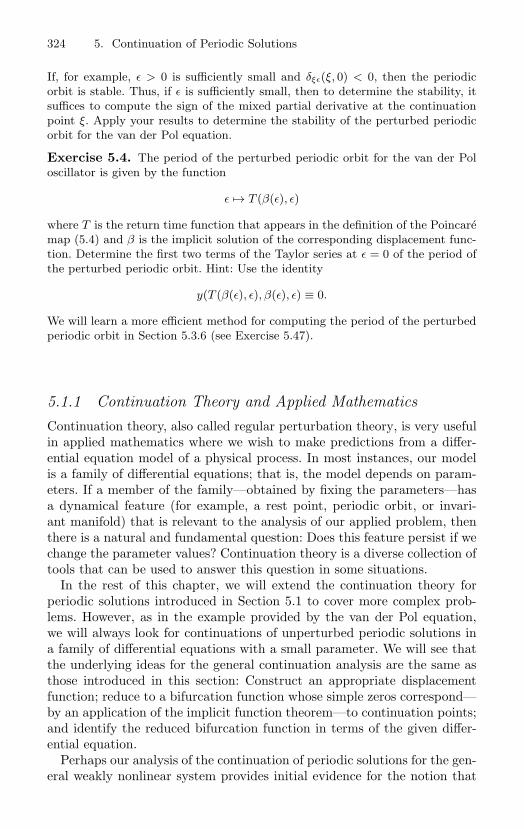
324 5. Continuation of Periodic Solutions
If, for example, ε > 0 is sufficiently small and δξε(ξ, 0) < 0, then the periodicorbit is stable. Thus, if ε is sufficiently small, then to determine the stability, itsuffices to compute the sign of the mixed partial derivative at the continuationpoint ξ. Apply your results to determine the stability of the perturbed periodicorbit for the van der Pol equation.
Exercise 5.4. The period of the perturbed periodic orbit for the van der Poloscillator is given by the function
ε → T (β(ε), ε)
where T is the return time function that appears in the definition of the Poincaremap (5.4) and β is the implicit solution of the corresponding displacement func-tion. Determine the first two terms of the Taylor series at ε = 0 of the period ofthe perturbed periodic orbit. Hint: Use the identity
y(T (β(ε), ε), β(ε), ε) ≡ 0.
We will learn a more efficient method for computing the period of the perturbedperiodic orbit in Section 5.3.6 (see Exercise 5.47).
5.1.1 Continuation Theory and Applied MathematicsContinuation theory, also called regular perturbation theory, is very usefulin applied mathematics where we wish to make predictions from a differ-ential equation model of a physical process. In most instances, our modelis a family of differential equations; that is, the model depends on param-eters. If a member of the family—obtained by fixing the parameters—hasa dynamical feature (for example, a rest point, periodic orbit, or invari-ant manifold) that is relevant to the analysis of our applied problem, thenthere is a natural and fundamental question: Does this feature persist if wechange the parameter values? Continuation theory is a diverse collection oftools that can be used to answer this question in some situations.
In the rest of this chapter, we will extend the continuation theory forperiodic solutions introduced in Section 5.1 to cover more complex prob-lems. However, as in the example provided by the van der Pol equation,we will always look for continuations of unperturbed periodic solutions ina family of differential equations with a small parameter. We will see thatthe underlying ideas for the general continuation analysis are the same asthose introduced in this section: Construct an appropriate displacementfunction; reduce to a bifurcation function whose simple zeros correspond—by an application of the implicit function theorem—to continuation points;and identify the reduced bifurcation function in terms of the given differ-ential equation.
Perhaps our analysis of the continuation of periodic solutions for the gen-eral weakly nonlinear system provides initial evidence for the notion that
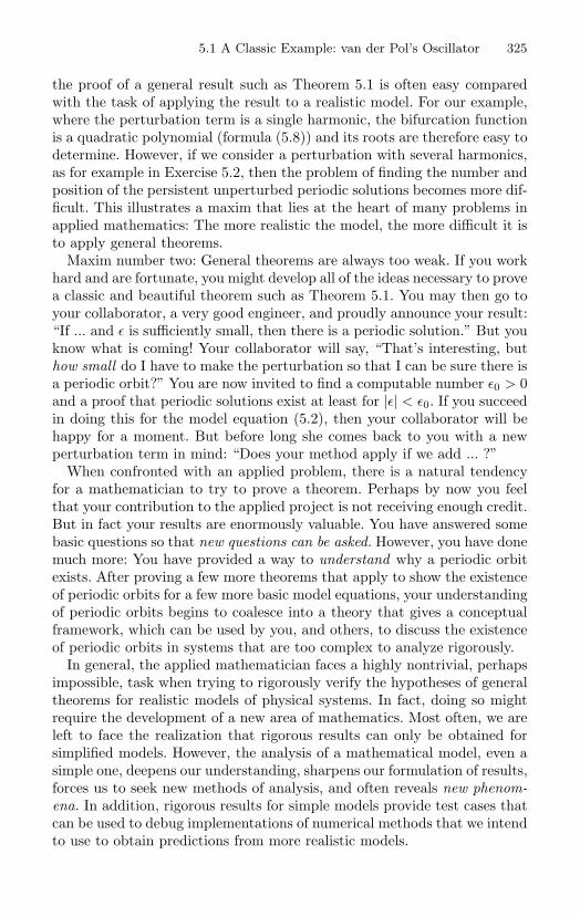
5.1 A Classic Example: van der Pol’s Oscillator 325
the proof of a general result such as Theorem 5.1 is often easy comparedwith the task of applying the result to a realistic model. For our example,where the perturbation term is a single harmonic, the bifurcation functionis a quadratic polynomial (formula (5.8)) and its roots are therefore easy todetermine. However, if we consider a perturbation with several harmonics,as for example in Exercise 5.2, then the problem of finding the number andposition of the persistent unperturbed periodic solutions becomes more dif-ficult. This illustrates a maxim that lies at the heart of many problems inapplied mathematics: The more realistic the model, the more difficult it isto apply general theorems.
Maxim number two: General theorems are always too weak. If you workhard and are fortunate, you might develop all of the ideas necessary to provea classic and beautiful theorem such as Theorem 5.1. You may then go toyour collaborator, a very good engineer, and proudly announce your result:“If ... and ε is sufficiently small, then there is a periodic solution.” But youknow what is coming! Your collaborator will say, “That’s interesting, buthow small do I have to make the perturbation so that I can be sure there isa periodic orbit?” You are now invited to find a computable number ε0 > 0and a proof that periodic solutions exist at least for |ε| < ε0. If you succeedin doing this for the model equation (5.2), then your collaborator will behappy for a moment. But before long she comes back to you with a newperturbation term in mind: “Does your method apply if we add ... ?”
When confronted with an applied problem, there is a natural tendencyfor a mathematician to try to prove a theorem. Perhaps by now you feelthat your contribution to the applied project is not receiving enough credit.But in fact your results are enormously valuable. You have answered somebasic questions so that new questions can be asked. However, you have donemuch more: You have provided a way to understand why a periodic orbitexists. After proving a few more theorems that apply to show the existenceof periodic orbits for a few more basic model equations, your understandingof periodic orbits begins to coalesce into a theory that gives a conceptualframework, which can be used by you, and others, to discuss the existenceof periodic orbits in systems that are too complex to analyze rigorously.
In general, the applied mathematician faces a highly nontrivial, perhapsimpossible, task when trying to rigorously verify the hypotheses of generaltheorems for realistic models of physical systems. In fact, doing so mightrequire the development of a new area of mathematics. Most often, we areleft to face the realization that rigorous results can only be obtained forsimplified models. However, the analysis of a mathematical model, even asimple one, deepens our understanding, sharpens our formulation of results,forces us to seek new methods of analysis, and often reveals new phenom-ena. In addition, rigorous results for simple models provide test cases thatcan be used to debug implementations of numerical methods that we intendto use to obtain predictions from more realistic models.
326 5. Continuation of Periodic Solutions
When we return as mathematicians to confront a realistic model of ouroriginal physical problem (the understanding of which is the real object ofthe game), it is not always clear how to continue doing mathematics. In-stead, we turn to computation and investigate numerical methods. Perhapswe become experts in computer algebra, or we investigate computer graph-ics in order to find useful visual representations of our data, and so on. Butwhen our simulations are implemented, we are happy to have knowledge ofthe range of expected phenomena, we are happy to be able to test our codeon the simplified models we have rigorously analyzed, and we are happyto verify numerically the hypotheses of a general theorem that we haveproved. All of this helps us gain confidence in our predictions.
By running our simulations, we find evidence for an answer to our origi-nal physical question. But during the process, we might also see unexpectedresults or we conceive new ideas to improve our simulations. These experi-ences motivate us to find additional rigorous results. Thus, we are naturallyled back to questions in mathematics. And so it goes—a natural cycle thatwill be repeated many times during our attempts to understand physicalphenomena.
Our technical skills will improve and our depth of understanding willincrease as we master more sophisticated mathematical methods and learnfrom the experience of doing applied mathematics. The remainder of thischapter is intended to help provide an example of an area of applicablemathematics as well as the opportunity to gain some useful experience withsome types of differential equations that appear as mathematical models.
5.2 Autonomous Perturbations
In this section we will consider the periodic solutions of the system
u = f(u) + εg(u), u ∈ R2 (5.10)
where ε is a small parameter and the unperturbed system
u = f(u) (5.11)
has periodic solutions. If the unperturbed differential equation (5.11) isnonlinear, then there are at least two cases to consider in our search forperiodic solutions of system (5.10): system (5.11) has a limit cycle (seeDefinition 1.119); and system (5.11) has an (invariant) annulus of periodicsolutions. In the limit cycle case, we wish to determine if the limit cyclepersists after perturbation; in the case of an invariant annulus of periodicsolutions, we wish to determine which, if any, of its constituent periodicsolutions persist.
Let us begin with the general assumption that the unperturbed sys-tem (5.11) has a periodic solution Γ. To employ the method suggested in
5.2 Autonomous Perturbations 327
Section 5.1, we must define a displacement function. To do this, let uschoose a point v ∈ Γ and a curve Σ1 that is transverse to Γ at v. Byan application of the implicit function theorem, there is an open segmentΣ ⊆ Σ1 with v ∈ Σ and some ε0 > 0 such that for each σ ∈ Σ the so-lution of the system (5.10) with |ε| < ε0 that has initial value σ returnsto Σ1 after some finite positive time. More precisely, there is a returntime function T : Σ × (−ε0, ε0) → R and a (parametrized) Poincare mapP : Σ × (−ε0, ε0) → Σ1. The subset Σ ⊆ Σ1 is called a Poincare section.
The usual definitions of Poincare section and Poincare map do not men-tion a parametrized system. However, the important point in the definitionof the Poincare section Σ is that solutions starting in Σ return to Σ1. Let usalso note that for each ε in the interval (−ε0, ε0) the corresponding Poincaremap σ → P (σ, ε) is defined on the fixed Poincare section Σ.
In the example in Section 5.1, the Poincare section is a line. Here, byallowing the Poincare section Σ to be a curve, we create a new technicalproblem: What is the definition of displacement on the manifold Σ? Thereare at least two options. We could define ∆ : Σ × (−ε0, ε0) → R
2 by∆(σ, ε) := P (σ, ε) − σ. However, if we do so, then the “displacement” is avector in R
2. Alternatively, if we view Σ1 as a one-dimensional manifold,then we can define the displacement function δ : R× (−ε0, ε0) → R relativeto a local coordinate representation of Σ. Indeed, let us choose a functionσ : R → Σ ⊆ R
2 such that σ(0) = v and for each ξ ∈ R the vector σ(ξ)is a nonzero tangent vector to Σ at σ(ξ). A displacement function is thendefined by
δ(ξ, ε) := σ−1(P (σ(ξ), ε)) − ξ. (5.12)
If we want to avoid local coordinates, then our naıve notion of distancewill have to be replaced by some measure of distance on the manifold Σ.This could be a reason to study differential geometry! The introduction ofmanifolds might seem unnecessarily complex, and certainly, the mention ofmanifolds and local coordinates can be avoided as long as the discussionis about curves. However, for generalizations of our continuation theory tohigher dimensional problems, these ideas are unavoidable. However, even inthe one-dimensional case, since we will have to compute partial derivativesof the displacement, we must ultimately make some choice of local coordi-nates. Hence, we may as well make this choice at the outset. Let us alsonote that our analysis is based on the implicit function theorem. For thisreason, it is advantageous to study a function R×R → R, the usual contextfor the implicit function theorem, rather than a function R×R → R
2. Thus,we will work with the definition of displacement given by equation (5.12).
Consider the case where the unperturbed system (5.11) has a limit cycleΓ with period 2π/ω and let δ be defined as in equation (5.12). We haveδ(0, 0) = 0. Also, because Γ is isolated among periodic solutions of thesystem (5.11), the function ξ → δ(ξ, 0) does not vanish in some puncturedneighborhood of ξ = 0. Thus, in this case the function δ is already in a
328 5. Continuation of Periodic Solutions
form where the implicit function theorem can be directly applied. In fact,we have the following proposition: If δξ(0, 0) = 0, then Γ persists. Theconclusion means that there is a continuous function ε → β(ε) defined insome interval containing ε = 0 with β(0) = 0 and δ(β(ε), ε) ≡ 0. Also,it is easy to identify δξ(0, 0). By the definition given in equation (5.12),the number δξ(0, 0) + 1 is the local representative of the derivative of thePoincare map on Σ at v = Γ∩Σ. In other words, δξ(0, 0) = 0 if and onlyif the derivative of the Poincare map is not the identity at v. A periodicorbit in the plane with this property is called hyperbolic. More generally, aperiodic orbit Γ is hyperbolic if the derivative of the Poincare map at v hasno eigenvalue with modulus one.
To identify δξ(0, 0) in terms of the function f , let
t → u(t, ζ, ε), ζ ∈ R2, ε ∈ R
denote the solution of system (5.10) with initial condition u(0, ζ, ε) = ζ, anddefine the local representation of the return time map T : R×(−ε0, ε0) → R
by T (ξ, ε) = T (σ(ξ), ε). From the definition of the displacement in dis-play (5.12), we have
σ(δ(ξ, ε) + ξ) = P (σ(ξ), ε) = u(T (ξ, ε), σ(ξ), ε). (5.13)
Set ε = 0 and note that ξ → σ(δ(ξ, ε)+ξ) defines a curve in Σ1 ⊆ R2. After
differentiation with respect to ξ at ξ = 0, we obtain an equality betweentangent vectors to Σ at v. In fact,
(δξ(0, 0) + 1)σ(0) = u(T (0, 0), v, 0)Tξ(0, 0) + uζ(T (0, 0), v, 0)σ(0)= Tξ(0, 0)f(v) + uζ(2π/ω, v, 0)σ(0). (5.14)
To be (absolutely) precise, the left hand side is
σ∗(0)[(δξ(0, 0) + 1)
∂
∂ξ
]where ∂
∂ξ denotes the unit tangent vector to R at ξ = 0 and σ∗(0) is thelinear map given by the differential of σ. This differential is a linear mapfrom the tangent space of R at ξ = 0 to the tangent space of Σ at v. Werepresent this quantity as a vector in R
2 that is tangent to Σ at v:
σ∗(0)(δξ(0, 0) + 1)∂
∂ξ= (δξ(0, 0) + 1)σ∗(0)
∂
∂ξ= (δξ(0, 0) + 1)σ(0).
Similar remarks apply to the identifications made on the right hand side.An expression for δξ(0, 0) can be determined from equation (5.14) once
we compute the derivative uζ(2π/ω, v, 0). Let us note that by taking thepartial derivative with respect to ζ in the equations
u(t, ζ, 0) = f(u(t, ζ, 0)), u(0, ζ, 0) = ζ,
5.2 Autonomous Perturbations 329
it is easy to see that the function t → uζ(t, ζ, 0) is the matrix solutionof the homogeneous variational equation (also called the first variationalequation) given by
W = Df(u(t, ζ, 0))W (5.15)
with initial condition W (0) = I where Df denotes the derivative of thefunction f . In other words, t → uζ(t, ζ, 0) is the principal fundamentalmatrix solution of the system (5.15) at t = 0 and the desired derivativeuζ(2π/ω, v, 0) is just the value of the solution of the variational initialvalue problem at t = 2π/ω.
Let ϕt(ζ) := u(t, ζ, 0) denote the flow of the differential equation (5.11)and let t → Φ(t) denote the principal fundamental matrix solution of thesystem (5.15) at t = 0. If f(ζ) = 0 (as it is in the present case becauseζ ∈ Γ and Γ is a periodic orbit), then the vectors f(ϕt(ζ)) and f⊥(ϕt(ζ)) arelinearly independent for each t ∈ R. The following additional propositionis simple but fundamental:
Φ(t)f(ζ) = f(ϕt(ζ)).
To prove it, note that Φ(0)f(ζ) = f(ζ) and
d
dtf(ϕt(ζ)) = Df(ϕt(ζ))f(ϕt(ζ)).
Thus, t → f(ϕt(ζ)) and t → Φ(t)f(ζ) are solutions of the same initial valueproblem, and therefore they must be equal.
Define f⊥ = Rf where R is the rotation matrix(
0 −11 0
). Since f and
f⊥ are linearly independent at each point of the plane where f is nonzero,there are two real-valued functions t → a(t, ζ) and t → b(t, ζ) such that
Φ(t)f⊥(ζ) = a(t, ζ)f(ϕt(ζ)) + b(t, ζ)f⊥(ϕt(ζ)). (5.16)
We will soon find useful formulas for a and b. However, using the definitionsjust given, let us note that the fundamental matrix Φ(t) is represented asa linear transformation from R
2, with the basis f(ζ), f⊥(ζ), to R2, with
the basis f(ϕt(ζ)), f⊥(ϕt(ζ)), by the matrix
Φ(t) =(
1 a(t, ζ)0 b(t, ζ)
). (5.17)
In equation (5.14), σ(0) is a tangent vector at v ∈ Σ ⊆ R2. Hence, there
are real constants c1 and c2 such that
σ(0) = c1f(v) + c2f⊥(v),
and therefore
(δξ(0, 0) + 1)(c1f(v) + c2f⊥(v))
= Tξ(0, 0)f(v) + Φ(2π/ω)(c1f(v) + c2f⊥(v))
= Tξ(0, 0)f(v) + c1f(v) + c2a(2π/ω, v)f(v) + c2b(2π/ω, v)f⊥(v).
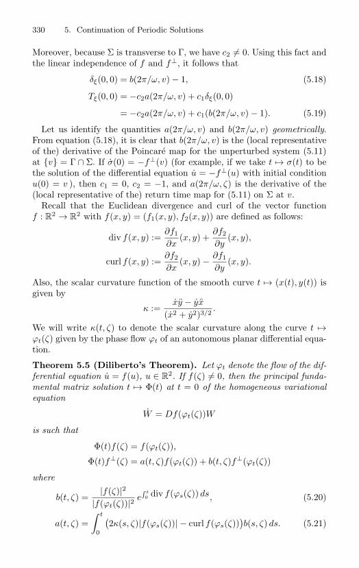
330 5. Continuation of Periodic Solutions
Moreover, because Σ is transverse to Γ, we have c2 = 0. Using this fact andthe linear independence of f and f⊥, it follows that
δξ(0, 0) = b(2π/ω, v) − 1, (5.18)
Tξ(0, 0) = −c2a(2π/ω, v) + c1δξ(0, 0)
= −c2a(2π/ω, v) + c1(b(2π/ω, v) − 1). (5.19)
Let us identify the quantities a(2π/ω, v) and b(2π/ω, v) geometrically.From equation (5.18), it is clear that b(2π/ω, v) is the (local representativeof the) derivative of the Poincare map for the unperturbed system (5.11)at v = Γ ∩ Σ. If σ(0) = −f⊥(v) (for example, if we take t → σ(t) to bethe solution of the differential equation u = −f⊥(u) with initial conditionu(0) = v ), then c1 = 0, c2 = −1, and a(2π/ω, ζ) is the derivative of the(local representative of the) return time map for (5.11) on Σ at v.
Recall that the Euclidean divergence and curl of the vector functionf : R
2 → R2 with f(x, y) = (f1(x, y), f2(x, y)) are defined as follows:
div f(x, y) :=∂f1
∂x(x, y) +
∂f2
∂y(x, y),
curl f(x, y) :=∂f2
∂x(x, y) − ∂f1
∂y(x, y).
Also, the scalar curvature function of the smooth curve t → (x(t), y(t)) isgiven by
κ :=xy − yx
(x2 + y2)3/2 .
We will write κ(t, ζ) to denote the scalar curvature along the curve t →ϕt(ζ) given by the phase flow ϕt of an autonomous planar differential equa-tion.
Theorem 5.5 (Diliberto’s Theorem). Let ϕt denote the flow of the dif-ferential equation u = f(u), u ∈ R
2. If f(ζ) = 0, then the principal funda-mental matrix solution t → Φ(t) at t = 0 of the homogeneous variationalequation
W = Df(ϕt(ζ))W
is such that
Φ(t)f(ζ) = f(ϕt(ζ)),
Φ(t)f⊥(ζ) = a(t, ζ)f(ϕt(ζ)) + b(t, ζ)f⊥(ϕt(ζ))
where
b(t, ζ) =|f(ζ)|2
|f(ϕt(ζ))|2 e∫ t0 div f(ϕs(ζ)) ds, (5.20)
a(t, ζ) =∫ t
0
(2κ(s, ζ)|f(ϕs(ζ))| − curl f(ϕs(ζ))
)b(s, ζ) ds. (5.21)
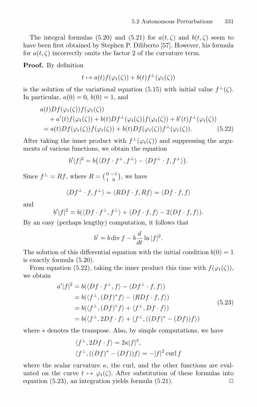
5.2 Autonomous Perturbations 331
The integral formulas (5.20) and (5.21) for a(t, ζ) and b(t, ζ) seem tohave been first obtained by Stephen P. Diliberto [57]. However, his formulafor a(t, ζ) incorrectly omits the factor 2 of the curvature term.
Proof. By definition
t → a(t)f(ϕt(ζ)) + b(t)f⊥(ϕt(ζ))
is the solution of the variational equation (5.15) with initial value f⊥(ζ).In particular, a(0) = 0, b(0) = 1, and
a(t)Df(ϕt(ζ))f(ϕt(ζ))+ a′(t)f(ϕt(ζ)) + b(t)Df⊥(ϕt(ζ))f(ϕt(ζ)) + b′(t)f⊥(ϕt(ζ))
= a(t)Df(ϕt(ζ))f(ϕt(ζ)) + b(t)Df(ϕt(ζ))f⊥(ϕt(ζ)). (5.22)
After taking the inner product with f⊥(ϕt(ζ)) and suppressing the argu-ments of various functions, we obtain the equation
b′|f |2 = b(〈Df · f⊥, f⊥〉 − 〈Df⊥ · f, f⊥〉
).
Since f⊥ = Rf , where R =( 0 −1
1 0
), we have
〈Df⊥ · f, f⊥〉 = 〈RDf · f, Rf〉 = 〈Df · f, f〉
andb′|f |2 = b(〈Df · f⊥, f⊥〉 + 〈Df · f, f〉 − 2〈Df · f, f〉).
By an easy (perhaps lengthy) computation, it follows that
b′ = b div f − bd
dtln |f |2.
The solution of this differential equation with the initial condition b(0) = 1is exactly formula (5.20).
From equation (5.22), taking the inner product this time with f(ϕt(ζ)),we obtain
a′|f |2 = b(〈Df · f⊥, f〉 − 〈Df⊥ · f, f〉)= b(〈f⊥, (Df)∗f〉 − 〈RDf · f, f〉)= b(〈f⊥, (Df)∗f〉 + 〈f⊥, Df · f〉)= b(〈f⊥, 2Df · f〉 + 〈f⊥, ((Df)∗ − (Df))f〉)
(5.23)
where ∗ denotes the transpose. Also, by simple computations, we have
〈f⊥, 2Df · f〉 = 2κ|f |3,〈f⊥, ((Df)∗ − (Df))f〉 = −|f |2 curl f
where the scalar curvature κ, the curl, and the other functions are eval-uated on the curve t → ϕt(ζ). After substitution of these formulas intoequation (5.23), an integration yields formula (5.21).
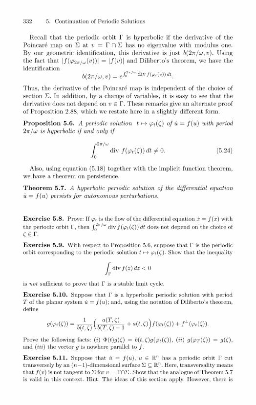
332 5. Continuation of Periodic Solutions
Recall that the periodic orbit Γ is hyperbolic if the derivative of thePoincare map on Σ at v = Γ ∩ Σ has no eigenvalue with modulus one.By our geometric identification, this derivative is just b(2π/ω, v). Usingthe fact that |f(ϕ2π/ω(v))| = |f(v)| and Diliberto’s theorem, we have theidentification
b(2π/ω, v) = e∫ 2π/ω0 div f(ϕt(v)) dt.
Thus, the derivative of the Poincare map is independent of the choice ofsection Σ. In addition, by a change of variables, it is easy to see that thederivative does not depend on v ∈ Γ. These remarks give an alternate proofof Proposition 2.88, which we restate here in a slightly different form.
Proposition 5.6. A periodic solution t → ϕt(ζ) of u = f(u) with period2π/ω is hyperbolic if and only if∫ 2π/ω
0div f(ϕt(ζ)) dt = 0. (5.24)
Also, using equation (5.18) together with the implicit function theorem,we have a theorem on persistence.
Theorem 5.7. A hyperbolic periodic solution of the differential equationu = f(u) persists for autonomous perturbations.
Exercise 5.8. Prove: If ϕt is the flow of the differential equation x = f(x) withthe periodic orbit Γ, then
∫ 2π/ω
0 div f(ϕt(ζ)) dt does not depend on the choice ofζ ∈ Γ.
Exercise 5.9. With respect to Proposition 5.6, suppose that Γ is the periodicorbit corresponding to the periodic solution t → ϕt(ζ). Show that the inequality
∫Γ
div f(z) dz < 0
is not sufficient to prove that Γ is a stable limit cycle.
Exercise 5.10. Suppose that Γ is a hyperbolic periodic solution with periodT of the planar system u = f(u); and, using the notation of Diliberto’s theorem,define
g(ϕt(ζ)) =1
b(t, ζ)
( a(T, ζ)b(T, ζ) − 1
+ a(t, ζ))f(ϕt(ζ)) + f⊥(ϕt(ζ)).
Prove the following facts: (i) Φ(t)g(ζ) = b(t, ζ)g(ϕt(ζ)), (ii) g(ϕT (ζ)) = g(ζ),and (iii) the vector g is nowhere parallel to f .
Exercise 5.11. Suppose that u = f(u), u ∈ Rn has a periodic orbit Γ cut
transversely by an (n−1)-dimensional surface Σ ⊆ Rn. Here, transversality means
that f(v) is not tangent to Σ for v = Γ∩Σ. Show that the analogue of Theorem 5.7is valid in this context. Hint: The ideas of this section apply. However, there is
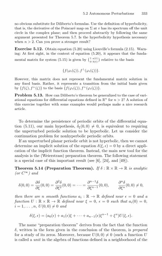
5.2 Autonomous Perturbations 333
no obvious substitute for Diliberto’s formulas. Use the definition of hyperbolicity,that is, the derivative of the Poincare map on Σ at v has its spectrum off the unitcircle in the complex plane; and then proceed abstractly by following the sameargument presented for Theorem 5.7. Is the hyperbolicity hypothesis necessarywhen n > 2. Can you prove a stronger result?
Exercise 5.12. Obtain equation (5.20) using Liouville’s formula (2.15). Warn-ing: At first sight, in the context of equation (5.20), it appears that the funda-
mental matrix for system (5.15) is given by( 1 a(t)
0 b(t)
)relative to the basis
f(ϕt(ζ)), f⊥(ϕt(ζ)).
However, this matrix does not represent the fundamental matrix solution inany fixed basis. Rather, it represents a transition from the initial basis givenby f(ζ), f⊥(ζ) to the basis f(ϕt(ζ)), f⊥(ϕt(ζ)).
Problem 5.13. How can Diliberto’s theorem be generalized to the case of vari-ational equations for differential equations defined in R
n for n > 2? A solution ofthis exercise together with some examples would perhaps make a nice researcharticle.
To determine the persistence of periodic orbits of the differential equa-tion (5.11), our main hypothesis, δξ(0, 0) = 0, is equivalent to requiringthe unperturbed periodic solution to be hyperbolic. Let us consider thecontinuation problem for nonhyperbolic periodic orbits.
If an unperturbed planar periodic orbit is not hyperbolic, then we cannotdetermine an implicit solution of the equation δ(ξ, ε) = 0 by a direct appli-cation of the implicit function theorem. Instead, the main new tool for theanalysis is the (Weierstrass) preparation theorem. The following statementis a special case of this important result (see [6], [24], and [49]).
Theorem 5.14 (Preparation Theorem). If δ : R × R → R is analytic(or C∞) and
δ(0, 0) =∂δ
∂ξ(0, 0) =
∂2δ
∂ξ2 (0, 0) = · · · =∂n−1δ
∂ξn−1 (0, 0),∂nδ
∂ξn(0, 0) = 0,
then there are n smooth functions ai : R → R defined near ε = 0 and afunction U : R × R → R defined near ξ = 0, ε = 0 such that ai(0) = 0,i = 1, . . . , n, U(0, 0) = 0 and
δ(ξ, ε) = (a0(ε) + a1(ε)ξ + · · · + an−1(ε)ξn−1 + ξn)U(ξ, ε).
The name “preparation theorem” derives from the fact that the functionδ, written in the form given in the conclusion of the theorem, is preparedfor a study of its zeros. Moreover, because U(0, 0) = 0 (such a function Uis called a unit in the algebra of functions defined in a neighborhood of the
334 5. Continuation of Periodic Solutions
origin), the zeros of the function δ(ξ, ε) near (ξ, ε) = (0, 0) are exactly thezeros of the Weierstrass polynomial
a0(ε) + a1(ε)ξ + · · · + an−1(ε)ξn−1 + ξn.
In particular, there are at most n zeros for each fixed ε near ε = 0.For the case where δ is the displacement function associated with a pe-
riodic orbit Γ, the multiplicity of Γ is defined to be the degree n of theWeierstrass polynomial. If n = 1, then Γ is hyperbolic and exactly onecontinuation point of periodic solutions exists for |ε| = 0 sufficiently small.It follows from the preparation theorem that if Γ has multiplicity n, thenthere is some choice of the function g in the differential equation (5.10) suchthat n families of periodic solutions bifurcate from Γ at ε = 0. However, foreach specific perturbation, the actual number of continuations can only bedetermined by analyzing the coefficients of the Weierstrass polynomial.
Exercise 5.15. Show that the system
x = −y + x(x2 + y2 − 1)2,
y = x + y(x2 + y2 − 1)2 (5.25)
has a limit cycle with multiplicity 2.
As an illustration of the ideas just presented, let us analyze the contin-uation problem for a periodic orbit Γ with multiplicity 2.
Using the displacement function δ associated with Γ, we have that
δ(0, 0) = δξ(0, 0) = 0, δξξ(0, 0) = 0,
and, by the preparation theorem,
δ(ξ, ε) = (a0(ε) + a1(ε)ξ + ξ2)U(ξ, ε) (5.26)
where a0(0) = 0, a1(0) = 0, but U(0, 0) = 0. We will solve for ξ implicitlywith respect to ε. But, in anticipation of a bifurcation at ε = 0, we cannotexpect to have a smooth continuation given by a function ε → β(ε) suchthat β(0) = 0 and δ(β(ε), ε) ≡ 0. More likely, there are implicit solutionsdefined for ε > 0 or ε < 0, but not both. For this reason, we say there are Npositive branches at the bifurcation point (0, 0) if there is some ε0 > 0 andN continuous functions β1, . . . , βN , each defined for 0 ≤ ε < ε0 such thatfor each j = 1, . . . , N , βj(0) = 0, and δ(βj(ε), ε) ≡ 0. Negative branches aredefined analogously for −ε0 < ε ≤ 0. Of course, the number and positionof the branches is determined by the roots of the Weierstrass polynomial.
With respect to the Weierstrass polynomial in display (5.26), we have
a0(ε) = a01ε + O(ε2), a1(ε) = O(ε),
5.2 Autonomous Perturbations 335
and therefore the roots of this Weierstrass polynomial are given by
ξ = β(ε) =−a1(ε) ±
√−4a01ε + O(ε2)2
.
If ε = 0 has fixed sign and a01ε > 0, then there are no real branches. Onthe other hand, if a01ε < 0, then there are two real branches given by
β1(ε) =√
−a01ε + O(ε), β2(ε) = −√
−a01ε + O(ε).
To identify the coefficient a01, compute the derivatives
δε(0, 0) = a01U(0, 0),δξξ(0, 0) = 2U(0, 0),
and note that
a01 = 2δε(0, 0)/δξξ(0, 0). (5.27)
Of course δξξ(0, 0) is just the second derivative of the unperturbed Poincaremap, that is, the map ξ → σ−1P (σ(ξ), 0). A formula for the derivativeδε(0, 0) will be computed below.
Let us apply the result in equation (5.27) to the bifurcation of limit cyclesfor the system
x = − y + x(x2 + y2 − 1)2,
y =x + y(x2 + y2 − 1)2 + ε(x2 − 1)y. (5.28)
By a change to polar coordinates, we have the equivalent system
r =r(r2 − 1)2 + εr sin2 θ(r2 cos2 θ − 1),
θ =1 + ε cos θ sin θ(r2 cos2 θ − 1).
Note that, for r near r = 1, if ε is sufficiently small, then we can treat θ asa time-like variable and obtain the following differential equation for r:
dr
dθ= F (r, θ, ε) :=
r(r2 − 1)2 + εr sin2 θ(r2 cos2 θ − 1)1 + ε cos θ sin θ(r2 cos2 θ − 1)
. (5.29)
Also, for each ξ near ξ = 1, let us define the function θ → r(θ, ξ, ε) to be theunique solution of the differential equation (5.29) with the initial conditionr(0, ξ, ε) = ξ.
Note that the displacement function is given by δ(ξ, ε) = r(2π, ξ, ε) − ξ.Thus, to compute the partial derivative δξ(ξ, ε), it suffices to solve thevariational initial value problem
rξ = Fr(r(θ, ξ, ε), ξ, ε)rξ, rξ(0, ξ, ε) = 1
336 5. Continuation of Periodic Solutions
to obtain the useful formula
rξ(θ, ξ, ε) = e∫ θ0 Fr(r(s,ξ,ε),ξ,ε) ds.
By Exercise 5.15, the point ξ = 1 corresponds to the unperturbed limitcycle. Thus, if we view ξ as a coordinate on the positive x-axis, thenδ(1, 0) = r(2π, 1, 0) − 1 = 0. Moreover, we have
rξ(2π, ξ, 0) = e∫ 2π0 (r2−1)(5r2−1) dθ,
and therefore δξ(1, 0) = 0. By taking one more derivative with respect toξ, let us note that
δξξ(1, 0) = rξξ(2π, 1, 0) =∫ 2π
08rξ dθ = e16π.
To compute δε(1, 0), solve the variational initial value problem
rε = r sin2 θ(r2 cos2 θ − 1), rε(0, 1, 0) = 0
to obtain
rε(2π, 1, 0) = −∫ 2π
0sin4 θ dθ < 0.
In particular, δε(1, 0) < 0, and, by using equation (5.27), we can concludethere are two branches of periodic solutions for small ε > 0. One branchconsists of stable limit cycles; the other branch consists of unstable limitcycles. We will outline the method for proving this fact, but the details areleft to the reader.
The stability of the perturbed limit cycles is determined by δξ(β(ε), ε). Infact, the orbit is unstable if δξ(β(ε), ε) > 0 and stable if δξ(β(ε), ε) < 0. Toprove this claim, recall that δ(ξ, ε) = σ−1(P (σ(ξ), ε)) − ξ and the stabilitytype is determined by the derivative of the Poincare map. Since δξ(0, 0) =0, the stability type for small ε is determined by the sign of δεξ(0, 0). Ifδεξ(0, 0) > 0 and a branch of continued periodic solutions exists for ε > 0,then the branch is unstable. If the branch exists for ε < 0, then the branchis stable. If δεξ(0, 0) < 0 and the branch exists for ε > 0, then it is stable,whereas, if the branch exists for ε < 0, then it is unstable.
We now have discussed a complete analysis for autonomous perturbationsin case Γ is hyperbolic, and we have just indicated how to approach theproblem when Γ has finite multiplicity. Let us consider the case where Γhas infinite multiplicity; that is, when δ(ξ, 0) ≡ 0. This, of course, is notquite correct if by infinite multiplicity we mean that all partial derivativesof the displacement function δ with respect to ξ vanish at (ξ, ε) = (0, 0);maybe δ is infinitely flat but still δ(ξ, 0) = 0 for ξ = 0. However, if δis analytic (it will be if the differential equation (5.10) is analytic), theninfinite multiplicity at the point ξ = 0 does imply that δ(ξ, 0) ≡ 0.
5.2 Autonomous Perturbations 337
Exercise 5.16. Give an example of an infinitely flat limit cycle: The periodicorbit is isolated but ∂kδ/∂ξk(0, 0) = 0 for k = 1, 2, 3, . . . .
Suppose that δ(ξ, 0) ≡ 0 and consider the perturbation series
δ(ξ, ε) = δε(ξ, 0)ε +12!
δεε(ξ, 0)ε2 + O(ε3).
Note that
δ(ξ, ε) = ε(δε(ξ, 0) + O(ε)). (5.30)
Here, since δ(ξ, 0) ≡ 0, the periodic orbit Γ is contained in a period annulus;that is, an annulus in the plane consisting entirely of periodic orbits of theunperturbed differential equation (5.11) (see, for example, Figure 3.2).
Although we could consider continuations from the fixed periodic orbitΓ, it is traditional to consider all of the periodic orbits in the period annu-lus together. Let us determine if any of the periodic orbits in the annuluspersist. For this problem, if we recall equation (5.30) and use the implicitfunction theorem, then the reduction step is easy: A simple zero of thefunction ξ → δε(ξ, 0) is a continuation point of periodic solutions. Equiva-lently, if δε(ξ0, 0) = 0 and δξε(ξ0, 0) = 0, then the periodic solution Γξ0 ofthe unperturbed system (5.11) with initial value σ(ξ0) ∈ Σ persists.
For the identification step, we will find a useful formula for δε(ξ, 0). Letus first compute the partial derivative with respect to ε in equation (5.13)to obtain the identity
δε(ξ, 0)σ(ξ) = Tε(ξ, 0)f(σ(ξ)) + uε(T (ξ, 0), σ(ξ), 0), (5.31)
and note that t → uε(t, σ(ξ), 0) is the solution of the inhomogeneous vari-ational initial value problem
W = Df(ϕt(σ(ξ)))W + g(ϕt(σ(ξ))), W (0) = 0, (5.32)
where the initial condition follows from the fact that u(0, σ(ξ), 0) ≡ σ(ξ).(The differential equation in display (5.32) is also called the second varia-tional equation.)
By the variation of constants formula,
uε(T (ξ, 0), σ(ξ), 0) = Φ(T (ξ, 0))∫ T (ξ,0)
0Φ−1(s)g(ϕs(σ(ξ))) ds
where Φ(t) denotes the principal fundamental matrix solution of the sys-tem (5.15) at t = 0.
Let us use the identifications given in equations (5.20) and (5.21) by firstexpressing the function g in the form
g(ϕt(σ(ξ))) = c1(t, σ(ξ))f(ϕt(σ(ξ))) + c2(t, σ(ξ))f⊥(ϕt(σ(ξ)))
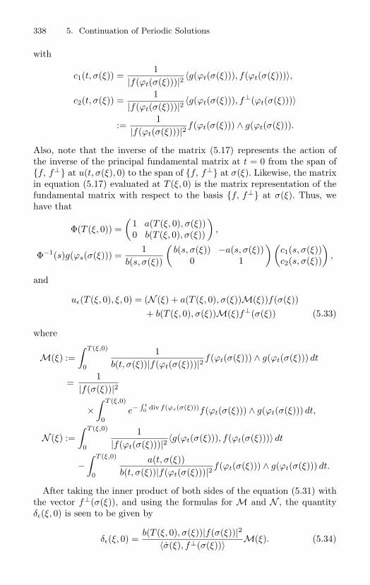
338 5. Continuation of Periodic Solutions
with
c1(t, σ(ξ)) =1
|f(ϕt(σ(ξ)))|2 〈g(ϕt(σ(ξ))), f(ϕt(σ(ξ)))〉,
c2(t, σ(ξ)) =1
|f(ϕt(σ(ξ)))|2 〈g(ϕt(σ(ξ))), f⊥(ϕt(σ(ξ)))〉
:=1
|f(ϕt(σ(ξ)))|2 f(ϕt(σ(ξ))) ∧ g(ϕt(σ(ξ))).
Also, note that the inverse of the matrix (5.17) represents the action ofthe inverse of the principal fundamental matrix at t = 0 from the span off, f⊥ at u(t, σ(ξ), 0) to the span of f, f⊥ at σ(ξ). Likewise, the matrixin equation (5.17) evaluated at T (ξ, 0) is the matrix representation of thefundamental matrix with respect to the basis f, f⊥ at σ(ξ). Thus, wehave that
Φ(T (ξ, 0)) =(
1 a(T (ξ, 0), σ(ξ))0 b(T (ξ, 0), σ(ξ))
),
Φ−1(s)g(ϕs(σ(ξ))) =1
b(s, σ(ξ))
(b(s, σ(ξ)) −a(s, σ(ξ))
0 1
)(c1(s, σ(ξ))c2(s, σ(ξ))
),
and
uε(T (ξ, 0), ξ, 0) = (N (ξ) + a(T (ξ, 0), σ(ξ))M(ξ))f(σ(ξ))+ b(T (ξ, 0), σ(ξ))M(ξ)f⊥(σ(ξ)) (5.33)
where
M(ξ) :=∫ T (ξ,0)
0
1b(t, σ(ξ))|f(ϕt(σ(ξ)))|2 f(ϕt(σ(ξ))) ∧ g(ϕt(σ(ξ))) dt
=1
|f(σ(ξ))|2
×∫ T (ξ,0)
0e− ∫ t
0 div f(ϕs(σ(ξ)))f(ϕt(σ(ξ))) ∧ g(ϕt(σ(ξ))) dt,
N (ξ) :=∫ T (ξ,0)
0
1|f(ϕt(σ(ξ)))|2 〈g(ϕt(σ(ξ))), f(ϕt(σ(ξ)))〉 dt
−∫ T (ξ,0)
0
a(t, σ(ξ))b(t, σ(ξ))|f(ϕt(σ(ξ)))|2 f(ϕt(σ(ξ))) ∧ g(ϕt(σ(ξ))) dt.
After taking the inner product of both sides of the equation (5.31) withthe vector f⊥(σ(ξ)), and using the formulas for M and N , the quantityδε(ξ, 0) is seen to be given by
δε(ξ, 0) =b(T (ξ, 0), σ(ξ))|f(σ(ξ))|2
〈σ(ξ), f⊥(σ(ξ))〉 M(ξ). (5.34)
5.2 Autonomous Perturbations 339
In this formula, 〈σ, f⊥〉 = 0 because Σ is transverse to the unperturbedperiodic solutions, and b(t, ζ) = 0 because |f | does not vanish along theunperturbed periodic orbit.
The autonomous Poincare–Andronov–Melnikov function is defined by
M(ξ) :=∫ T (ξ,0)
0e− ∫ t
0 div f(ϕs(σ(ξ))) dsf(ϕt(σ(ξ))) ∧ g(ϕt(σ(ξ))) dt. (5.35)
Here, ξ → T (ξ, 0) is a local representation of the period function associatedwith the period annulus of the differential equation (5.11); the numberT (ξ, 0) is the minimum period of the periodic orbit labeled by ξ, that is,the orbit passing through the point in the plane with coordinates (ξ, 0).It should be clear that values of the function M are independent of thechoice of Poincare section. In fact, as long as ξ is a smooth parameter forthe periodic solutions in our period annulus, the value of M at a particularperiodic solution is not altered by the choice of the parametrization.
Theorem 5.17. Suppose that the differential equation (5.11) has a periodannulus A whose periodic solutions are parametrized by a smooth functionσ : R → A given by ξ → σ(ξ). If ξ0 is a simple zero of the functionξ → M(ξ) given by the formula (5.35) for the perturbed system (5.10),then the periodic solution of the unperturbed system (5.11) passing throughξ0 is continuable.
Proof. This result follows immediately from the formula (5.34) and thefact that simple zeros of ξ → δε(ξ, 0) persist. We only remark that, ingeneral, if α(ξ) = β(ξ)γ(ξ) with β(ξ) nonvanishing, then the simple zerosof α and γ coincide.
Exercise 5.18. Find the continuable periodic solutions of the perturbed har-monic oscillator in each of the following systems:
1. weakly damped van der Pol equation:
x + ε(x2 − 1)x + ω2x = 0;
2. nonlinear weakly damped van der Pol equation:
x + ε(x2 − 1)x + ω2x − ελx3 = 0;
3. modified van der Pol equation:
x + ε(x2 + x2 − 1)x + x = 0.
340 5. Continuation of Periodic Solutions
5.3 Nonautonomous Perturbations
Let us consider the periodic solutions of the nonautonomous periodicallyperturbed system
u = f(u) + εg(u, t, ε), u ∈ R2. (5.36)
More precisely, let us suppose that the unperturbed system has a periodicsolution Γ whose period is 2π/ω and that t → g(u, t, ε) is periodic withperiod
η := η(ε) =n
m
2π
ω+ kε + O(ε2) (5.37)
where n, m are relatively prime positive integers and k ∈ R is the “detuningparameter.” In particular, at ε = 0 we have
mη(0) = n2π
ω(5.38)
and we say that the periodic solution Γ is in (m : n) resonance with theperturbation g. Equation (5.38) is called a resonance relation. If, as before,we let t → u(t, ζ, ε) denote the solution of the differential equation (5.36)with initial condition u(0, ζ, ε) = ζ in R
2, then we have that t → u(t, ζ, 0)defines a 2π/ω-periodic function for each ζ ∈ Γ.
The nonautonomous differential equation (5.36) is equivalent to the firstorder system
u = f(u) + εg(u, τ, ε),τ = 1
(5.39)
in the extended phase plane. Due to the fact that g is a periodic functionof time, it is customary to view τ as an angular variable modulo η(ε). Thisleads to the very useful geometric interpretation of the system (5.39) as adifferential system on the phase cylinder R
2 × T where
T := e2πiτ/η(ε) : τ ∈ R.
There is an annular region A ⊆ R2 containing Γ and some ε0 > 0 such
that Σ = A×1 ⊆ R2 ×T is a Poincare section for the system (5.39) with
associated (parametrized) Poincare map P : Σ× (−ε0, ε0) → R2 defined by
(ζ, 1, ε) → u(η(ε), ζ, ε).
However, because the set A × 1 is naturally identified with A, we willview the Poincare map as the map P : A × (−ε0, ε0) → R
2 given by
(ζ, ε) → u(η(ε), ζ, ε). (5.40)
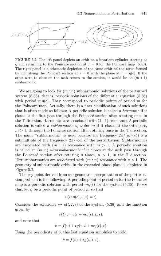
5.3 Nonautonomous Perturbations 341
u
FIGURE 5.2. The left panel depicts an orbit on a invariant cylinder starting atζ and returning to the Poincare section at τ = 0 for the Poincare map (5.40).The right panel is a schematic depiction of the same orbit on the torus formedby identifying the Poincare section at τ = 0 with the plane at τ = η(ε). If theorbit were to close on the mth return to the section, it would be an (m : 1)subharmonic.
We are going to look for (m : n) subharmonic solutions of the perturbedsystem (5.36), that is, periodic solutions of the differential equation (5.36)with period mη(ε). They correspond to periodic points of period m forthe Poincare map. Actually, there is a finer classification of such solutionsthat is often made as follows: A periodic solution is called a harmonic if itcloses at the first pass through the Poincare section after rotating once inthe T direction. Harmonics are associated with (1 : 1) resonance. A periodicsolution is called a subharmonic of order m if it closes at the mth pass,m > 1, through the Poincare section after rotating once in the T direction.The name “subharmonic” is used because the frequency 2π/(mη(ε)) is asubmultiple of the frequency 2π/η(ε) of the perturbation. Subharmonicsare associated with (m : 1) resonance with m > 1. A periodic solutionis called an (m, n) ultrasubharmonic if it closes at the mth pass throughthe Poincare section after rotating n times, n > 1, in the T direction.Ultrasubharmonics are associated with (m : n) resonance with n > 1. Thegeometry of subharmonic orbits in the extended phase plane is depicted inFigure 5.2.
The key point derived from our geometric interpretation of the perturba-tion problem is the following: A periodic point of period m for the Poincaremap is a periodic solution with period mη(ε) for the system (5.36). To seethis, let ζ be a periodic point of period m so that
u(mη(ε), ζ, t) = ζ.
Consider the solution t → u(t, ζ, ε) of the system (5.36) and the functiongiven by
v(t) := u(t + mη(ε), ζ, ε),
and note thatv = f(v) + εg(v, t + mη(ε), ε).
Using the periodicity of g, this last equation simplifies to yield
v = f(v) + εg(v, t, ε),
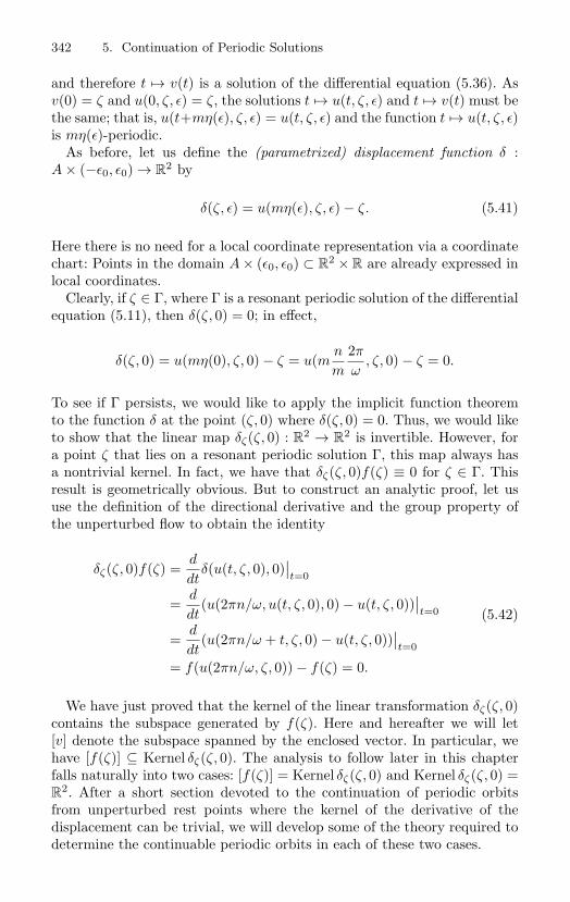
342 5. Continuation of Periodic Solutions
and therefore t → v(t) is a solution of the differential equation (5.36). Asv(0) = ζ and u(0, ζ, ε) = ζ, the solutions t → u(t, ζ, ε) and t → v(t) must bethe same; that is, u(t+mη(ε), ζ, ε) = u(t, ζ, ε) and the function t → u(t, ζ, ε)is mη(ε)-periodic.
As before, let us define the (parametrized) displacement function δ :A × (−ε0, ε0) → R
2 by
δ(ζ, ε) = u(mη(ε), ζ, ε) − ζ. (5.41)
Here there is no need for a local coordinate representation via a coordinatechart: Points in the domain A × (ε0, ε0) ⊂ R
2 × R are already expressed inlocal coordinates.
Clearly, if ζ ∈ Γ, where Γ is a resonant periodic solution of the differentialequation (5.11), then δ(ζ, 0) = 0; in effect,
δ(ζ, 0) = u(mη(0), ζ, 0) − ζ = u(mn
m
2π
ω, ζ, 0) − ζ = 0.
To see if Γ persists, we would like to apply the implicit function theoremto the function δ at the point (ζ, 0) where δ(ζ, 0) = 0. Thus, we would liketo show that the linear map δζ(ζ, 0) : R
2 → R2 is invertible. However, for
a point ζ that lies on a resonant periodic solution Γ, this map always hasa nontrivial kernel. In fact, we have that δζ(ζ, 0)f(ζ) ≡ 0 for ζ ∈ Γ. Thisresult is geometrically obvious. But to construct an analytic proof, let ususe the definition of the directional derivative and the group property ofthe unperturbed flow to obtain the identity
δζ(ζ, 0)f(ζ) =d
dtδ(u(t, ζ, 0), 0)
∣∣t=0
=d
dt(u(2πn/ω, u(t, ζ, 0), 0) − u(t, ζ, 0))
∣∣t=0
=d
dt(u(2πn/ω + t, ζ, 0) − u(t, ζ, 0))
∣∣t=0
= f(u(2πn/ω, ζ, 0)) − f(ζ) = 0.
(5.42)
We have just proved that the kernel of the linear transformation δζ(ζ, 0)contains the subspace generated by f(ζ). Here and hereafter we will let[v] denote the subspace spanned by the enclosed vector. In particular, wehave [f(ζ)] ⊆ Kernel δζ(ζ, 0). The analysis to follow later in this chapterfalls naturally into two cases: [f(ζ)] = Kernel δζ(ζ, 0) and Kernel δζ(ζ, 0) =R
2. After a short section devoted to the continuation of periodic orbitsfrom unperturbed rest points where the kernel of the derivative of thedisplacement can be trivial, we will develop some of the theory required todetermine the continuable periodic orbits in each of these two cases.
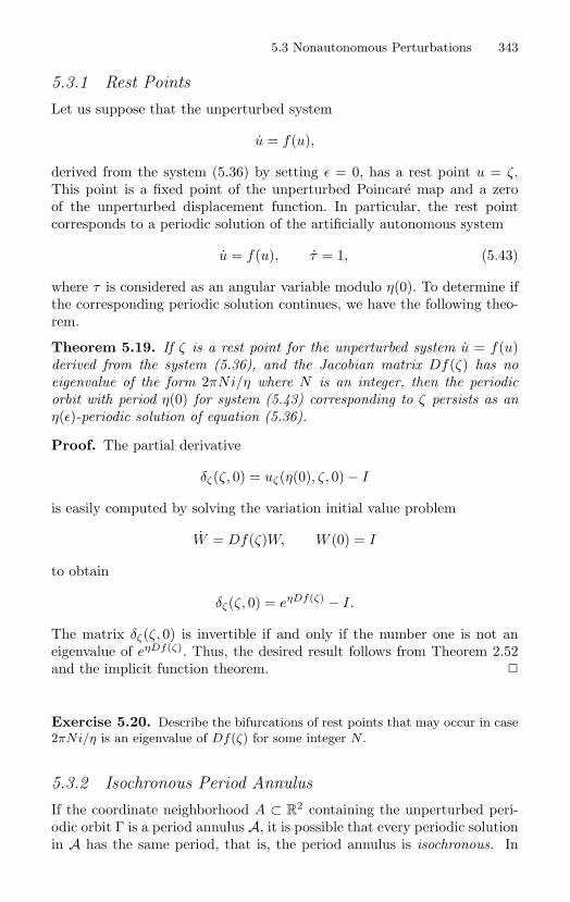
5.3 Nonautonomous Perturbations 343
5.3.1 Rest PointsLet us suppose that the unperturbed system
u = f(u),
derived from the system (5.36) by setting ε = 0, has a rest point u = ζ.This point is a fixed point of the unperturbed Poincare map and a zeroof the unperturbed displacement function. In particular, the rest pointcorresponds to a periodic solution of the artificially autonomous system
u = f(u), τ = 1, (5.43)
where τ is considered as an angular variable modulo η(0). To determine ifthe corresponding periodic solution continues, we have the following theo-rem.
Theorem 5.19. If ζ is a rest point for the unperturbed system u = f(u)derived from the system (5.36), and the Jacobian matrix Df(ζ) has noeigenvalue of the form 2πNi/η where N is an integer, then the periodicorbit with period η(0) for system (5.43) corresponding to ζ persists as anη(ε)-periodic solution of equation (5.36).
Proof. The partial derivative
δζ(ζ, 0) = uζ(η(0), ζ, 0) − I
is easily computed by solving the variation initial value problem
W = Df(ζ)W, W (0) = I
to obtain
δζ(ζ, 0) = eηDf(ζ) − I.
The matrix δζ(ζ, 0) is invertible if and only if the number one is not aneigenvalue of eηDf(ζ). Thus, the desired result follows from Theorem 2.52and the implicit function theorem.
Exercise 5.20. Describe the bifurcations of rest points that may occur in case2πNi/η is an eigenvalue of Df(ζ) for some integer N .
5.3.2 Isochronous Period AnnulusIf the coordinate neighborhood A ⊂ R
2 containing the unperturbed peri-odic orbit Γ is a period annulus A, it is possible that every periodic solutionin A has the same period, that is, the period annulus is isochronous. In
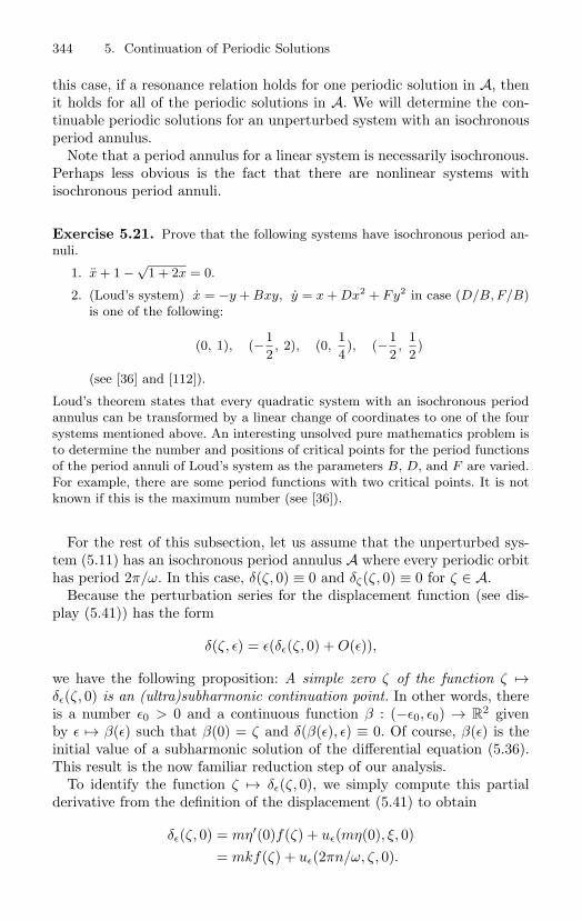
344 5. Continuation of Periodic Solutions
this case, if a resonance relation holds for one periodic solution in A, thenit holds for all of the periodic solutions in A. We will determine the con-tinuable periodic solutions for an unperturbed system with an isochronousperiod annulus.
Note that a period annulus for a linear system is necessarily isochronous.Perhaps less obvious is the fact that there are nonlinear systems withisochronous period annuli.
Exercise 5.21. Prove that the following systems have isochronous period an-nuli.
1. x + 1 − √1 + 2x = 0.
2. (Loud’s system) x = −y + Bxy, y = x + Dx2 + Fy2 in case (D/B, F/B)is one of the following:
(0, 1), (−12, 2), (0,
14), (−1
2,
12)
(see [36] and [112]).
Loud’s theorem states that every quadratic system with an isochronous periodannulus can be transformed by a linear change of coordinates to one of the foursystems mentioned above. An interesting unsolved pure mathematics problem isto determine the number and positions of critical points for the period functionsof the period annuli of Loud’s system as the parameters B, D, and F are varied.For example, there are some period functions with two critical points. It is notknown if this is the maximum number (see [36]).
For the rest of this subsection, let us assume that the unperturbed sys-tem (5.11) has an isochronous period annulus A where every periodic orbithas period 2π/ω. In this case, δ(ζ, 0) ≡ 0 and δζ(ζ, 0) ≡ 0 for ζ ∈ A.
Because the perturbation series for the displacement function (see dis-play (5.41)) has the form
δ(ζ, ε) = ε(δε(ζ, 0) + O(ε)),
we have the following proposition: A simple zero ζ of the function ζ →δε(ζ, 0) is an (ultra)subharmonic continuation point. In other words, thereis a number ε0 > 0 and a continuous function β : (−ε0, ε0) → R
2 givenby ε → β(ε) such that β(0) = ζ and δ(β(ε), ε) ≡ 0. Of course, β(ε) is theinitial value of a subharmonic solution of the differential equation (5.36).This result is the now familiar reduction step of our analysis.
To identify the function ζ → δε(ζ, 0), we simply compute this partialderivative from the definition of the displacement (5.41) to obtain
δε(ζ, 0) = mη′(0)f(ζ) + uε(mη(0), ξ, 0)= mkf(ζ) + uε(2πn/ω, ζ, 0).
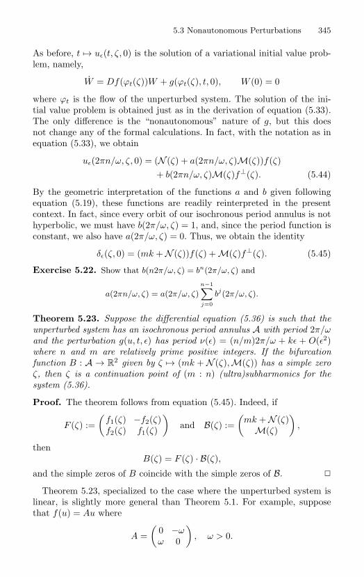
5.3 Nonautonomous Perturbations 345
As before, t → uε(t, ζ, 0) is the solution of a variational initial value prob-lem, namely,
W = Df(ϕt(ζ))W + g(ϕt(ζ), t, 0), W (0) = 0
where ϕt is the flow of the unperturbed system. The solution of the ini-tial value problem is obtained just as in the derivation of equation (5.33).The only difference is the “nonautonomous” nature of g, but this doesnot change any of the formal calculations. In fact, with the notation as inequation (5.33), we obtain
uε(2πn/ω, ζ, 0) = (N (ζ) + a(2πn/ω, ζ)M(ζ))f(ζ)+ b(2πn/ω, ζ)M(ζ)f⊥(ζ). (5.44)
By the geometric interpretation of the functions a and b given followingequation (5.19), these functions are readily reinterpreted in the presentcontext. In fact, since every orbit of our isochronous period annulus is nothyperbolic, we must have b(2π/ω, ζ) = 1, and, since the period function isconstant, we also have a(2π/ω, ζ) = 0. Thus, we obtain the identity
δε(ζ, 0) = (mk + N (ζ))f(ζ) + M(ζ)f⊥(ζ). (5.45)
Exercise 5.22. Show that b(n2π/ω, ζ) = bn(2π/ω, ζ) and
a(2πn/ω, ζ) = a(2π/ω, ζ)n−1∑j=0
bj(2π/ω, ζ).
Theorem 5.23. Suppose the differential equation (5.36) is such that theunperturbed system has an isochronous period annulus A with period 2π/ωand the perturbation g(u, t, ε) has period ν(ε) = (n/m)2π/ω + kε + O(ε2)where n and m are relatively prime positive integers. If the bifurcationfunction B : A → R
2 given by ζ → (mk + N (ζ),M(ζ)) has a simple zeroζ, then ζ is a continuation point of (m : n) (ultra)subharmonics for thesystem (5.36).
Proof. The theorem follows from equation (5.45). Indeed, if
F (ζ) :=(
f1(ζ) −f2(ζ)f2(ζ) f1(ζ)
)and B(ζ) :=
(mk + N (ζ)
M(ζ)
),
thenB(ζ) = F (ζ) · B(ζ),
and the simple zeros of B coincide with the simple zeros of B.
Theorem 5.23, specialized to the case where the unperturbed system islinear, is slightly more general than Theorem 5.1. For example, supposethat f(u) = Au where
A =(
0 −ωω 0
), ω > 0.
346 5. Continuation of Periodic Solutions
Since div f ≡ 0 and |f | is constant on orbits, b(t, ζ) ≡ 1. Also, let us notethat
2κ(t, ζ)|f(ϕt(ζ))| − curl f(ϕt(ζ)) = 21|ζ|ω|ζ| − 2ω = 0,
and therefore a(t, ζ) ≡ 0. (This is a good internal check that the formulafor a is correct!) Thus, in this special case,
N (ζ) =∫ n2π/ω
0
1|f(ϕt(ζ))|2 〈f(ϕt(ζ)), g(ϕt(ζ), t, 0)〉 dt,
M(ζ) =1
|f(ζ)|2∫ n2π/ω
0f(ϕt(ζ)) ∧ g(ϕt(ζ), t, 0) dt.
More explicitly, we have that
N (ζ) =1
ω|ζ|2∫ n2π/ω
0xg2(x, y, t, 0) − yg1(x, y, t, 0) dt,
M(ζ) = − 1ω|ζ|2
∫ n2π/ω
0xg1(x, y, t, 0) + yg2(x, y, t, 0) dt (5.46)
where
x := x(t, ζ) = ζ1 cos ωt − ζ2 sin ωt, y := y(t, ζ) = ζ1 sin ωt + ζ2 cos ωt.
Let us consider the stability of the perturbed (ultra)subharmonics. Notethat the “perturbation series” for the Poincare map is given by
P (ζ, ε) = ζ + εPε(ζ, 0) + O(ε2),
and Pε(ζ, 0) = δε(ζ, 0). Thus, the formula for the partial derivative of thePoincare map with respect to ε is given by equation (5.45) and
P (ζ, ε) =(
ζ1ζ2
)+ ε
(kmω
(−ζ2ζ1
)+
(∫ n2π/ω
0 g1 cos ωt + g2 sin wt dt∫ n2π/ω
0 g2 cos ωt − g1 sin wt dt
))+ O(ε2) (5.47)
where g1 and g2 are evaluated at (x, y, t, 0).It should be clear that the stability of the perturbed (ultra)subharmonics
is determined by the eigenvalues of the matrix Pζ(ζ, ε), called the linearizedPoincare map evaluated at the fixed point of ζ → P (ζ, ε) correspond-ing to the subharmonic. The subharmonic is stable if both eigenvalues lieinside the unit circle in the complex plane. Of course, if the linearizedPoincare map is hyperbolic, then the local behavior near the periodic orbitis determined—stability is just a special case of this more general fact.
5.3 Nonautonomous Perturbations 347
It is not too difficult to show that if ε > 0 is sufficiently small, thenthe matrix Pζ(ζ, ε) evaluated at the perturbed fixed point has both of itseigenvalues inside the unit circle in the complex plane provided that eacheigenvalue of the matrix Pζε(ζ, 0) has negative real part. For ε < 0, eacheigenvalue of the matrix Pζε(ζ, 0) must have positive real part. Equivalently,it suffices to have
det Pζε(ζ, 0) > 0, ε trPζε(ζ, 0) < 0.
The proof of this fact contains a pleasant surprise.The perturbation series for the Poincare map evaluated along the curve
ε → (β(ε), ε) has the form
Pζ(β(ε), ε) = I + εA + ε2B + O(ε3)
where A = Pζε(β(0), 0). In particular, we have used the fact that Pζζ(ζ, 0) =0. The characteristic polynomial of the first order approximation of thismatrix, namely, I + εA, has coefficients that contain terms of second orderin ε. Thus, it appears that second order terms in the perturbation seriesare required for computing the eigenvalues to first order. However, there isan unexpected cancellation, and the eigenvalues, for ε > 0, are given by
1 + ε12(trA ±
√tr2 A − 4 det A
)+ O(ε2). (5.48)
Using formula (5.48), it is easy to show that if the eigenvalues of A havenonzero real parts, then the first order terms of the expansion determinethe stability. If A has an eigenvalue with zero real part, then higher orderterms in the perturbation expansion must be considered (see [131]).
General formulas for the eigenvalues of Pζε(ζ, 0) can be obtained in termsof certain partial derivatives of M and N . However, such formulas areusually not useful. A better approach is to use the special properties of thesystem under investigation.
Exercise 5.24. Prove the statements following equation (5.48) concerning theeigenvalues of the matrix Pζ(ζ, ε).
5.3.3 The Forced van der Pol OscillatorIn this subsection we will outline, by formulating a series of exercises, someapplications of the continuation theory (developed so far in this chapter)to the classic case of the van der Pol oscillator. Also, we mention brieflysome of the additional structures that can be studied using our first ordermethods.
348 5. Continuation of Periodic Solutions
Exercise 5.25. Find the (ultra)subharmonics for the periodically forced vander Pol oscillator
x + ε(x2 − 1)x + x = εa sinΩt.
In particular, for fixed a = 0, find the regions in (Ω, ε) space near the line ε = 0where (ultra)subharmonics exist.
The regions mentioned in Exercise 5.25 are called entrainment domainsor, in some of the electrical engineering literature, they are called synchro-nization domains. We cannot determine the entire extent of the entrain-ment domains because our first order theory is only valid for sufficientlysmall |ε|. Higher order methods can be used to obtain more information(see, for example, [124] and [86], and for some classic numerical experiments[89]).
To use the formulas for M and N in display (5.46), let us consider thefirst order system in the phase plane given by
x = −y, y = x + ε(−(x2 − 1)y − a sin Ωt).
Also, let us consider curves in the (Ω, ε) parameter space of the form ε →(Ω(ε), ε) where
Ω(ε) =m
n− k
(m
n
)2ε + O(ε2),
η(ε) = 2πn
m+ kε + O(ε2).
To complete Exercise 5.25, start by looking for harmonics; that is, lookfor periodic solutions of the perturbed system with periods close to 2π forΩ near Ω = 1. Set m = n = 1. To help debug the computations for thisexample, first try the case k = 0 where k is the detuning, and show thatthere is a harmonic at the point (ζ1, ζ2) provided that ζ2 = 0 and ζ1 is aroot of the equation ζ3
1 −4ζ1 +4a = 0. This corresponds to perturbation inthe vertical direction in the parameter space. Show that the harmonic willbe stable if |ζ1| > 2 and that there is a unique (stable) harmonic in casea = 1.
There is a very interesting difference between the (1 : 1) resonance andthe (m : n) resonance with m/n = 1. To glimpse into this structure, con-sider the (m : n) resonance where m/n = 1 and use equation (5.47) tocompute the following first order approximation of the associated Poincaremap:
ζ1 → ζ1 + ε(
− kmζ2 + nπζ1 − nπ
4ζ1(ζ2
1 + ζ22 )
),
ζ2 → ζ2 + ε(kmζ1 + nπζ2 − nπ
4ζ2(ζ2
1 + ζ22 )
). (5.49)
5.3 Nonautonomous Perturbations 349
This map preserves the origin. Thus, it is natural to study the map in polarcoordinates where it is represented to first order by
r → r + εnπr(1 − r2
4
),
θ → θ + εmk. (5.50)
Here the first order formula in the rectangular coordinates goes over toa formula in polar coordinates that contains higher order terms in ε thathave been deleted. Can we safely ignore these higher order terms?
For the (1 : 1) resonance with k included as a parameter, a similar firstorder computation yields the map
ζ1 → ζ1 + ε(
− kζ2 + πζ1 − aπ − π
4ζ1(ζ2
1 + ζ22 )
),
ζ2 → ζ2 + ε(kζ1 + πζ2 − π
4ζ2(ζ2
1 + ζ22 )
). (5.51)
Note that if this map preserves the origin, then a = 0. Thus, polar coor-dinates are not the natural coordinates for studying this map. However, auseful representation of the map is obtained by changing to the complexcoordinate z = ζ1 + iζ2 where the map is represented in the form
z → z + ε((π + ki)z − 1
4πz2z − aπ
). (5.52)
We will that show the dynamics of the map defined in display (5.49) arequite different from the dynamics of the map in display (5.51).
For the map (5.50), the circle r = 2 is an invariant set and every pointin the plane except the origin is attracted to this circle under iteration. Onthe circle, the map gives a rational or an irrational rotation depending onwhether or not k is rational. In other words, an analysis of the dynamicsat this approximation suggests that there is an invariant torus in the phasespace of the differential equation and solutions of the differential equationthat do not start on the torus are attracted at an exponential rate tothis torus in positive time. Roughly speaking, such an invariant torus iscalled normally hyperbolic; for the precise definition of normal hyperbolicitysee [64] and [94].
Solutions of the differential equation on the invariant torus may windaround the torus, as in the case of irrational rotation, or they may beattracted to a subharmonic on the torus as in the case of rational rotation.There are general theorems that can be used to show that a normallyhyperbolic torus will persist with the addition of a small perturbation (see,for example, [64], [83], and [94], and also [34] and [40]). Thus, we see thatthere is a second possible type of entrainment. It is possible that solutionsare entrained to the torus when there are no periodic solutions on the torus.In this case, corresponding to an irrational rotation, every solution on the
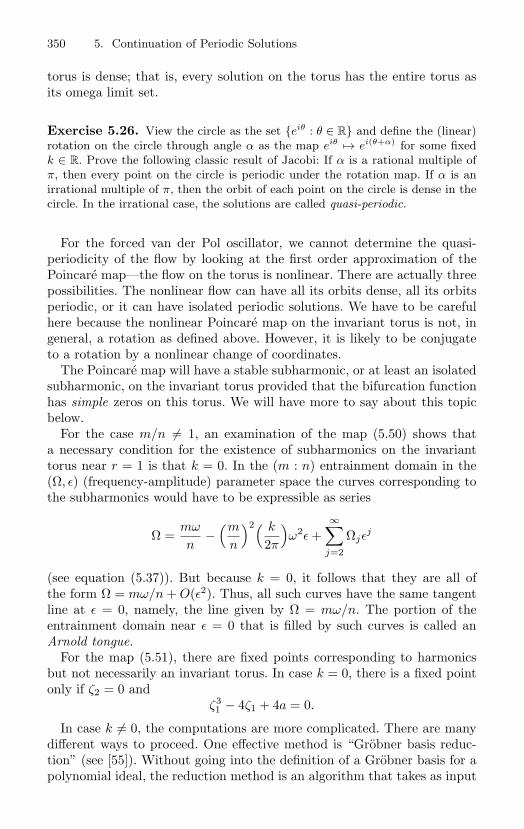
350 5. Continuation of Periodic Solutions
torus is dense; that is, every solution on the torus has the entire torus asits omega limit set.
Exercise 5.26. View the circle as the set eiθ : θ ∈ R and define the (linear)rotation on the circle through angle α as the map eiθ → ei(θ+α) for some fixedk ∈ R. Prove the following classic result of Jacobi: If α is a rational multiple ofπ, then every point on the circle is periodic under the rotation map. If α is anirrational multiple of π, then the orbit of each point on the circle is dense in thecircle. In the irrational case, the solutions are called quasi-periodic.
For the forced van der Pol oscillator, we cannot determine the quasi-periodicity of the flow by looking at the first order approximation of thePoincare map—the flow on the torus is nonlinear. There are actually threepossibilities. The nonlinear flow can have all its orbits dense, all its orbitsperiodic, or it can have isolated periodic solutions. We have to be carefulhere because the nonlinear Poincare map on the invariant torus is not, ingeneral, a rotation as defined above. However, it is likely to be conjugateto a rotation by a nonlinear change of coordinates.
The Poincare map will have a stable subharmonic, or at least an isolatedsubharmonic, on the invariant torus provided that the bifurcation functionhas simple zeros on this torus. We will have more to say about this topicbelow.
For the case m/n = 1, an examination of the map (5.50) shows thata necessary condition for the existence of subharmonics on the invarianttorus near r = 1 is that k = 0. In the (m : n) entrainment domain in the(Ω, ε) (frequency-amplitude) parameter space the curves corresponding tothe subharmonics would have to be expressible as series
Ω =mω
n−
(m
n
)2( k
2π
)ω2ε +
∞∑j=2
Ωjεj
(see equation (5.37)). But because k = 0, it follows that they are all ofthe form Ω = mω/n + O(ε2). Thus, all such curves have the same tangentline at ε = 0, namely, the line given by Ω = mω/n. The portion of theentrainment domain near ε = 0 that is filled by such curves is called anArnold tongue.
For the map (5.51), there are fixed points corresponding to harmonicsbut not necessarily an invariant torus. In case k = 0, there is a fixed pointonly if ζ2 = 0 and
ζ31 − 4ζ1 + 4a = 0.
In case k = 0, the computations are more complicated. There are manydifferent ways to proceed. One effective method is “Grobner basis reduc-tion” (see [55]). Without going into the definition of a Grobner basis for apolynomial ideal, the reduction method is an algorithm that takes as input
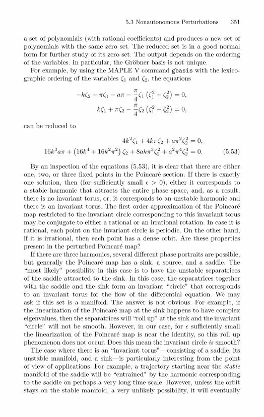
5.3 Nonautonomous Perturbations 351
a set of polynomials (with rational coefficients) and produces a new set ofpolynomials with the same zero set. The reduced set is in a good normalform for further study of its zero set. The output depends on the orderingof the variables. In particular, the Grobner basis is not unique.
For example, by using the MAPLE V command gbasis with the lexico-graphic ordering of the variables ζ1 and ζ2, the equations
−kζ2 + πζ1 − aπ − π
4ζ1
(ζ21 + ζ2
2)
= 0,
kζ1 + πζ2 − π
4ζ2
(ζ21 + ζ2
2)
= 0,
can be reduced to
4k2ζ1 + 4kπζ2 + aπ2ζ22 = 0,
16k3aπ +(16k4 + 16k2π2) ζ2 + 8akπ3ζ2
2 + a2π4ζ32 = 0. (5.53)
By an inspection of the equations (5.53), it is clear that there are eitherone, two, or three fixed points in the Poincare section. If there is exactlyone solution, then (for sufficiently small ε > 0), either it corresponds toa stable harmonic that attracts the entire phase space, and, as a result,there is no invariant torus, or, it corresponds to an unstable harmonic andthere is an invariant torus. The first order approximation of the Poincaremap restricted to the invariant circle corresponding to this invariant torusmay be conjugate to either a rational or an irrational rotation. In case it isrational, each point on the invariant circle is periodic. On the other hand,if it is irrational, then each point has a dense orbit. Are these propertiespresent in the perturbed Poincare map?
If there are three harmonics, several different phase portraits are possible,but generally the Poincare map has a sink, a source, and a saddle. The“most likely” possibility in this case is to have the unstable separatricesof the saddle attracted to the sink. In this case, the separatrices togetherwith the saddle and the sink form an invariant “circle” that correspondsto an invariant torus for the flow of the differential equation. We mayask if this set is a manifold. The answer is not obvious. For example, ifthe linearization of the Poincare map at the sink happens to have complexeigenvalues, then the separatrices will “roll up” at the sink and the invariant“circle” will not be smooth. However, in our case, for ε sufficiently smallthe linearization of the Poincare map is near the identity, so this roll upphenomenon does not occur. Does this mean the invariant circle is smooth?
The case where there is an “invariant torus”—consisting of a saddle, itsunstable manifold, and a sink—is particularly interesting from the pointof view of applications. For example, a trajectory starting near the stablemanifold of the saddle will be “entrained” by the harmonic correspondingto the saddle on perhaps a very long time scale. However, unless the orbitstays on the stable manifold, a very unlikely possibility, it will eventually
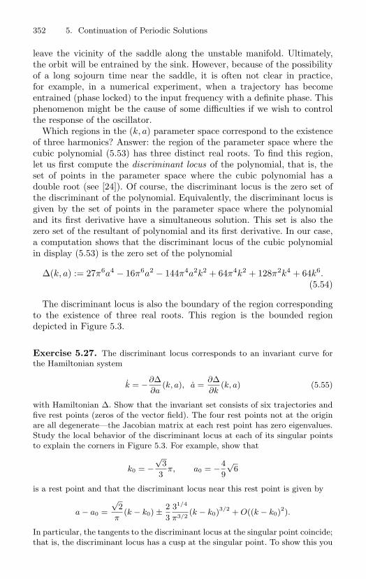
352 5. Continuation of Periodic Solutions
leave the vicinity of the saddle along the unstable manifold. Ultimately,the orbit will be entrained by the sink. However, because of the possibilityof a long sojourn time near the saddle, it is often not clear in practice,for example, in a numerical experiment, when a trajectory has becomeentrained (phase locked) to the input frequency with a definite phase. Thisphenomenon might be the cause of some difficulties if we wish to controlthe response of the oscillator.
Which regions in the (k, a) parameter space correspond to the existenceof three harmonics? Answer: the region of the parameter space where thecubic polynomial (5.53) has three distinct real roots. To find this region,let us first compute the discriminant locus of the polynomial, that is, theset of points in the parameter space where the cubic polynomial has adouble root (see [24]). Of course, the discriminant locus is the zero set ofthe discriminant of the polynomial. Equivalently, the discriminant locus isgiven by the set of points in the parameter space where the polynomialand its first derivative have a simultaneous solution. This set is also thezero set of the resultant of polynomial and its first derivative. In our case,a computation shows that the discriminant locus of the cubic polynomialin display (5.53) is the zero set of the polynomial
∆(k, a) := 27π6a4 − 16π6a2 − 144π4a2k2 + 64π4k2 + 128π2k4 + 64k6.(5.54)
The discriminant locus is also the boundary of the region correspondingto the existence of three real roots. This region is the bounded regiondepicted in Figure 5.3.
Exercise 5.27. The discriminant locus corresponds to an invariant curve forthe Hamiltonian system
k = −∂∆∂a
(k, a), a =∂∆∂k
(k, a) (5.55)
with Hamiltonian ∆. Show that the invariant set consists of six trajectories andfive rest points (zeros of the vector field). The four rest points not at the originare all degenerate—the Jacobian matrix at each rest point has zero eigenvalues.Study the local behavior of the discriminant locus at each of its singular pointsto explain the corners in Figure 5.3. For example, show that
k0 = −√
33
π, a0 = −49
√6
is a rest point and that the discriminant locus near this rest point is given by
a − a0 =√
2π
(k − k0) ± 23
31/4
π3/2 (k − k0)3/2 + O((k − k0)2).
In particular, the tangents to the discriminant locus at the singular point coincide;that is, the discriminant locus has a cusp at the singular point. To show this you
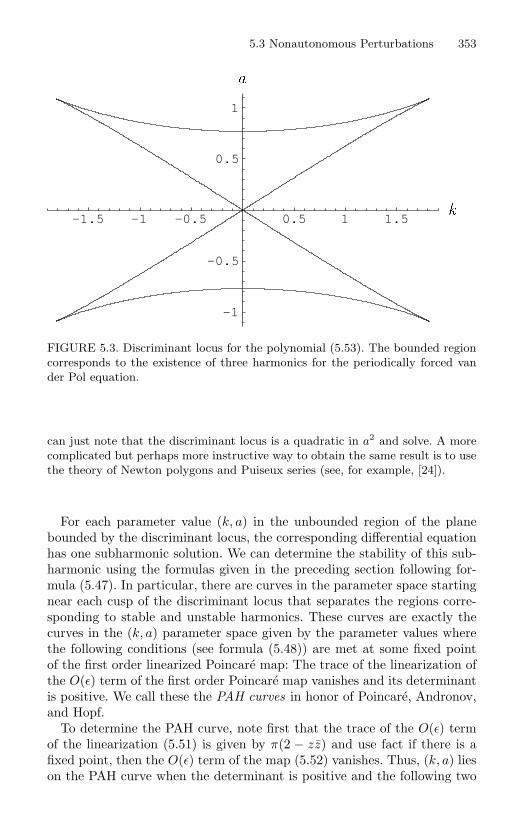
5.3 Nonautonomous Perturbations 353
-1.5 -1 -0.5 0.5 1 1.5
-1
-0.5
0.5
1
k
a
FIGURE 5.3. Discriminant locus for the polynomial (5.53). The bounded regioncorresponds to the existence of three harmonics for the periodically forced vander Pol equation.
can just note that the discriminant locus is a quadratic in a2 and solve. A morecomplicated but perhaps more instructive way to obtain the same result is to usethe theory of Newton polygons and Puiseux series (see, for example, [24]).
For each parameter value (k, a) in the unbounded region of the planebounded by the discriminant locus, the corresponding differential equationhas one subharmonic solution. We can determine the stability of this sub-harmonic using the formulas given in the preceding section following for-mula (5.47). In particular, there are curves in the parameter space startingnear each cusp of the discriminant locus that separates the regions corre-sponding to stable and unstable harmonics. These curves are exactly thecurves in the (k, a) parameter space given by the parameter values wherethe following conditions (see formula (5.48)) are met at some fixed pointof the first order linearized Poincare map: The trace of the linearization ofthe O(ε) term of the first order Poincare map vanishes and its determinantis positive. We call these the PAH curves in honor of Poincare, Andronov,and Hopf.
To determine the PAH curve, note first that the trace of the O(ε) termof the linearization (5.51) is given by π(2 − zz) and use fact if there is afixed point, then the O(ε) term of the map (5.52) vanishes. Thus, (k, a) lieson the PAH curve when the determinant is positive and the following two
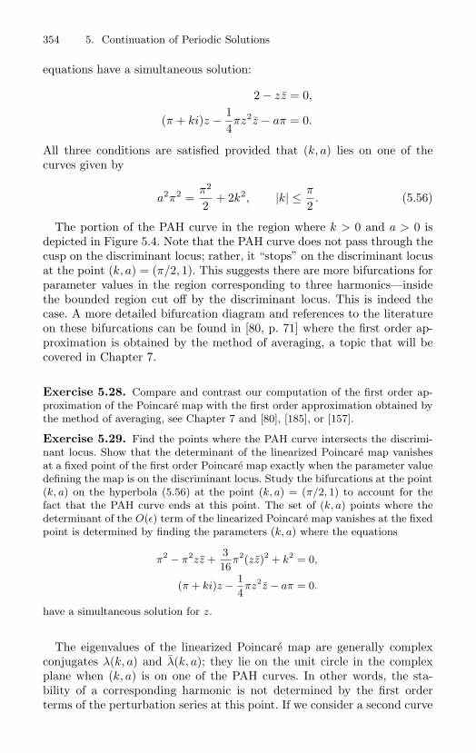
354 5. Continuation of Periodic Solutions
equations have a simultaneous solution:
2 − zz = 0,
(π + ki)z − 14πz2z − aπ = 0.
All three conditions are satisfied provided that (k, a) lies on one of thecurves given by
a2π2 =π2
2+ 2k2, |k| ≤ π
2. (5.56)
The portion of the PAH curve in the region where k > 0 and a > 0 isdepicted in Figure 5.4. Note that the PAH curve does not pass through thecusp on the discriminant locus; rather, it “stops” on the discriminant locusat the point (k, a) = (π/2, 1). This suggests there are more bifurcations forparameter values in the region corresponding to three harmonics—insidethe bounded region cut off by the discriminant locus. This is indeed thecase. A more detailed bifurcation diagram and references to the literatureon these bifurcations can be found in [80, p. 71] where the first order ap-proximation is obtained by the method of averaging, a topic that will becovered in Chapter 7.
Exercise 5.28. Compare and contrast our computation of the first order ap-proximation of the Poincare map with the first order approximation obtained bythe method of averaging, see Chapter 7 and [80], [185], or [157].
Exercise 5.29. Find the points where the PAH curve intersects the discrimi-nant locus. Show that the determinant of the linearized Poincare map vanishesat a fixed point of the first order Poincare map exactly when the parameter valuedefining the map is on the discriminant locus. Study the bifurcations at the point(k, a) on the hyperbola (5.56) at the point (k, a) = (π/2, 1) to account for thefact that the PAH curve ends at this point. The set of (k, a) points where thedeterminant of the O(ε) term of the linearized Poincare map vanishes at the fixedpoint is determined by finding the parameters (k, a) where the equations
π2 − π2zz +316
π2(zz)2 + k2 = 0,
(π + ki)z − 14πz2z − aπ = 0.
have a simultaneous solution for z.
The eigenvalues of the linearized Poincare map are generally complexconjugates λ(k, a) and λ(k, a); they lie on the unit circle in the complexplane when (k, a) is on one of the PAH curves. In other words, the sta-bility of a corresponding harmonic is not determined by the first orderterms of the perturbation series at this point. If we consider a second curve
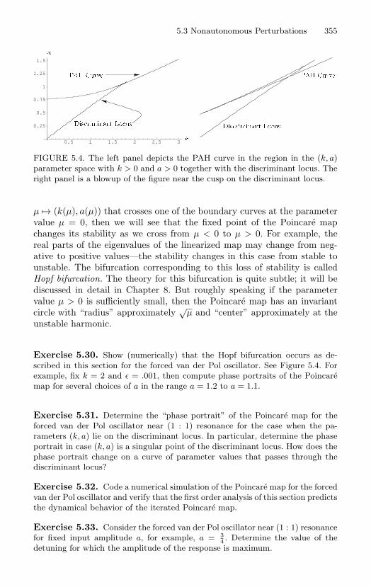
5.3 Nonautonomous Perturbations 355
0.5 1 1.5 2 2.5 3
0.25
0.5
0.75
1
1.25
1.5
PAH Curve
Discriminant Locus
PAH Curve
k
a
Discriminant Locus
FIGURE 5.4. The left panel depicts the PAH curve in the region in the (k, a)parameter space with k > 0 and a > 0 together with the discriminant locus. Theright panel is a blowup of the figure near the cusp on the discriminant locus.
µ → (k(µ), a(µ)) that crosses one of the boundary curves at the parametervalue µ = 0, then we will see that the fixed point of the Poincare mapchanges its stability as we cross from µ < 0 to µ > 0. For example, thereal parts of the eigenvalues of the linearized map may change from neg-ative to positive values—the stability changes in this case from stable tounstable. The bifurcation corresponding to this loss of stability is calledHopf bifurcation. The theory for this bifurcation is quite subtle; it will bediscussed in detail in Chapter 8. But roughly speaking if the parametervalue µ > 0 is sufficiently small, then the Poincare map has an invariantcircle with “radius” approximately
√µ and “center” approximately at the
unstable harmonic.
Exercise 5.30. Show (numerically) that the Hopf bifurcation occurs as de-scribed in this section for the forced van der Pol oscillator. See Figure 5.4. Forexample, fix k = 2 and ε = .001, then compute phase portraits of the Poincaremap for several choices of a in the range a = 1.2 to a = 1.1.
Exercise 5.31. Determine the “phase portrait” of the Poincare map for theforced van der Pol oscillator near (1 : 1) resonance for the case when the pa-rameters (k, a) lie on the discriminant locus. In particular, determine the phaseportrait in case (k, a) is a singular point of the discriminant locus. How does thephase portrait change on a curve of parameter values that passes through thediscriminant locus?
Exercise 5.32. Code a numerical simulation of the Poincare map for the forcedvan der Pol oscillator and verify that the first order analysis of this section predictsthe dynamical behavior of the iterated Poincare map.
Exercise 5.33. Consider the forced van der Pol oscillator near (1 : 1) resonancefor fixed input amplitude a, for example, a = 3
4 . Determine the value of thedetuning for which the amplitude of the response is maximum.
356 5. Continuation of Periodic Solutions
5.3.4 Regular Period AnnulusIn this section we will discuss a continuation theory for periodic solutionsof the periodically perturbed oscillator
u = f(u) + εg(u, t, ε), u ∈ R2, (5.57)
in case the unperturbed system has a resonant periodic orbit that is con-tained in a nonisochronous period annulus.
Consider an unperturbed resonant periodic orbit Γ for system (5.57)that is contained in a period annulus A, and recall that if A is isochronous,then all of the orbits in A are resonant and the unperturbed displacementfunction ζ → δ(ζ, 0), defined as in display (5.41) by
δ(ζ, ε) = u(mη(ε), ζ, ε) − ζ, (5.58)
vanishes identically. If A is not isochronous, then we expect that althoughthe unperturbed displacement function does vanish on Γ, it does not vanishon nearby periodic orbits.
What happens when we attempt to apply the implicit function theorem?For each z ∈ Γ we have δ(z, 0) = 0. If, in addition, the linear transformationδζ(z, 0) : R
2 → R2 were invertible, then z would be a continuation point.
But, as demonstrated by the result in display (5.42), this linear transfor-mation is not invertible. In particular, all vectors tangent to Γ are in itskernel.
In this section, we will consider the case where the kernel of the deriva-tive of the displacement function at each point z ∈ Γ is exactly the one-dimensional tangent space to Γ at z. In other words, we will assume thatKernel δζ(ζ, 0) = [f(ζ)]. If this condition is met, then Γ, as well as thecorresponding invariant torus for the system
u = f(u), τ = 1,
is called normally nondegenerate.Before proceeding to the continuation analysis, let us consider a geomet-
rical interpretation of our assumption about the kernel of the derivativeof the displacement function. For this, we do not need to assume that theperiodic orbit Γ is contained in a period annulus. Instead, we may assumemore generally that there is a region R ⊆ R
2 and an ε0 > 0 such that thedisplacement function δ : R × (−ε0, ε0) → R
2 is defined. Also, let us as-sume that there is a curve Σ ⊆ R transverse to Γ—a Poincare section—suchthat the return time map T : Σ × (−ε0, ε0) → R is defined. The followingproposition gives the geometrical conditions we seek.
Proposition 5.34. Suppose Γ is an (m : n) resonant unperturbed periodicsolution of the periodically perturbed oscillator (5.57); T : Σ × (−ε0, ε0) →R is the return time map defined on a Poincare section Σ with v =
5.3 Nonautonomous Perturbations 357
Γ ∩ Σ; and R ⊆ R2 is a region containing Γ such that for some ε0 > 0 the
displacement δ : R × (−ε0, ε0) → R2 given in equation (5.58) is defined. If
Γ is contained in a period annulus A ⊆ R such that the differential T∗(v, 0)of σ → T (σ, 0) at σ = v is nonsingular, then Kernel δζ(ζ, 0) = [f(ζ)] andRange δζ(ζ, 0) = [f(ζ)] for each ζ ∈ Γ. If Γ is a hyperbolic limit cycle,or if T∗(v, 0) is nonsingular, then Kernel δζ(ζ, 0) = [f(ζ)] for all ζ ∈ Γ.Moreover, if Σ is orthogonal to Γ at v, then
Range δζ(ζ, 0) = [r1f(ζ) + r2f⊥(ζ)]
for each ζ ∈ Γ where, for a and b as in Diliberto’s theorem (Theorem 5.5),
r1 = a(2πn/ω, v) = −n−1∑j=0
bj(2π/ω, v)(T∗(ζ, 0)f⊥(ζ)),
r2 = b(2πn/ω, v) − 1 = bn(2π/ω, v) − 1.
Proof. By equation (5.42), we have [f(ζ)] ⊆ Kernel δζ(ζ, 0). Consider thevector field f⊥ and the solution t → u⊥(t, ζ) of the initial value problem
u = f⊥(u), u(0) = ζ.
In other words u⊥(t, ζ) is the flow of f⊥. We have
δζ(ζ, 0)f⊥(ζ) =d
dt(u(mη(0), u⊥(t, ζ), 0) − u⊥(t, ζ))
∣∣∣t=0
= uζ(2πn/ω, ζ, 0)f⊥(ζ) − f⊥(ζ).
Here t → uζ(t, ζ, 0) is the principal fundamental matrix at t = 0 for thevariational equation (5.15). Thus, from equation (5.16) and Exercise 5.22we have
δζ(ζ, 0)f⊥(ζ) =( n−1∑
j=0
bj(2π/ω, v))a(2π/ω, v)f(ζ)
+(bn(2π/ω, v) − 1)f⊥(ζ). (5.59)
If Γ is contained in a period annulus, then b(2π/ω, v) = 1 and, by equa-tion (5.19),
a(2π/ω, v) = − |f(ζ)|2〈σ(0), f⊥(ζ)〉T ′(0)
where σ(0) is the tangent vector to Σ at ζ determined by the parametriza-tion of Σ. Thus,
δζ(ζ, 0)f⊥(ζ) = −n|f(ζ)|2
〈σ(0), f⊥(ζ)〉T ′(0)f(ζ) = 0
358 5. Continuation of Periodic Solutions
and Kernel δζ(ζ, 0) = [f(ζ)]. Also, the range of δζ(ζ, 0) is [f(ζ)].On the other hand, if Γ is a hyperbolic limit cycle, then b(2π/ω, v) = 1,
the coefficient of f⊥(ζ) in equation (5.59) does not vanish, and f⊥(ζ) /∈Kernel δζ(ζ, 0). Hence, in this case we have that Kernel δζ(ζ, 0) = [f(ζ)].Moreover, if Σ is orthogonal to Γ at ζ, then
δζ(ζ, 0)f⊥(ζ) =( n−1∑
j=0
bj(2π/ω, v))(
− T ′(0)|f(ζ)|2〈σ(0), f⊥(ζ)〉
)f(ζ)
+ (bn(2π/ω, v) − 1)f⊥(ζ).
We say that a period annulus A is a regular period annulus if the dif-ferential T∗(ζ, 0) of the return time, defined as in the previous theorem, isnonsingular at every point of A. Let us note that the differential T∗(ζ, 0) isnonsingular if and only if the corresponding period function for the periodannulus A has a nonvanishing derivative; that is, the period function isregular.
Every resonant periodic orbit contained in a regular period annulus isnormally nondegenerate. Also, by Proposition 5.34, if Γ is a resonant pe-riodic orbit in A and ζ ∈ Γ, then both the kernel and range of the partialderivative δζ(ζ, 0) are given by [f(ζ)]. In particular, if we restrict the lin-ear map δζ(ζ, 0) to [f⊥(ζ)], then the map δζ(ζ, 0) : [f⊥(ζ)] → [f(ζ)] is anisomorphism. We will use these facts in the analysis to follow.
Exercise 5.35. Prove that a linear map on a finite dimensional vector space,when restricted to a complement of its kernel, is an isomorphism onto its range.What happens in an infinite dimensional space?
Let us reiterate the basic fact that the partial derivative δζ(ζ, 0) of thedisplacement function, when viewed as a map on all of R
2, has a nontrivialkernel. This precludes a direct application of the implicit function theoremto solve the equation δ(ζ, ε) = 0 on R
2 × R. However, we can use theimplicit function theorem to reduce our search for continuation points tothe problem of solving a related equation on a lower dimensional space. Thisis accomplished by using an important technique called Lyapunov–Schmidtreduction. This method is very general. In fact, it works for equationsdefined on Banach spaces when the linear map playing the role of ourderivative δζ(ζ, 0) is a Fredholm operator. We will give a brief introductionto these simple but powerful ideas in an abstract setting. However, as wewill demonstrate when we apply the method to our continuation problem,it is very fruitful to keep the idea of the method firmly in mind, but itmay not be efficient to adapt all of the abstraction verbatim. Also, on afirst reading and for the applications to be made later in this section, it
5.3 Nonautonomous Perturbations 359
is sufficient to consider only finite dimensional real Banach spaces, that is,R
n with the usual norm.Let us suppose that B1 and B2 are Banach spaces and L(B1,B2) denotes
the bounded linear maps from B1 to B2. Also, with this notation, let usrecall that a map G : B1 → B2 is C1 if there is a continuous map L : B1 →L(B1,B2) such that
limn→0
‖G(x + h) − G(x) − L(x) · h‖‖h‖ = 0
for each x ∈ B1. A map A ∈ L(B1,B2) is called Fredholm if it has a finitedimensional kernel and a closed range with a finite dimensional comple-ment. The index of a Fredholm map is defined to be the difference of thedimensions of its corange and kernel.
Suppose that X and Y are open subsets of the Banach spaces B and Erespectively, and F : X × Y → B, given by (x, y) → F (x, y), is a C1 mapsuch that F (0, 0) = 0. Since F is C1, the partial derivative Fx(0, 0) is abounded linear map on B. However, let us assume in addition that Fx(0, 0)is Fredholm with index zero.
If B is finite dimensional, as in our application where F is the displace-ment function and B = R
2, then every linear map is automatically Fred-holm. Let us also note that we will use the hypothesis that our Fredholmmap has index zero to ensure that the final reduced bifurcation function isa map between finite dimensional spaces of the same dimension. However,the general Lyapunov–Schmidt reduction technique does not require theFredholm map to have index zero.
Let K denote the kernel of the Fredholm map Fx(0, 0), and let R de-note its range. There are subspaces KC and RC such that B = K ⊕ KCand B = R ⊕ RC. The complement RC exists by the Fredholm hypoth-esis. The existence of a complement KC for the finite dimensional kernelK in an infinite dimensional Banach space is a consequence of the Hahn–Banach theorem (see [156, p. 105]). Indeed, choose a basis for the finitedimensional subspace, apply the Hahn–Banach theorem to extend the cor-responding dual basis functionals to the entire Banach space, use the ex-tended functionals to define a projection from the entire space to the finitedimensional subspace, and construct the desired complement as the rangeof the complementary projection.
The complementary subspaces KC and RC are not unique. In fact, inthe applications, the correct choices for these spaces can be an importantissue. However, there are complementary linear projections P : B → R andQ : B → RC corresponding to the direct sum splitting of B. Also, there isa product neighborhood of the origin in X of the form U ×V where U ⊆ Kand V ⊆ KC.
360 5. Continuation of Periodic Solutions
Consider the map H : U×V ×Y → R defined by (u, v, y) → PF (u+v, y).Its partial derivative with respect to v at (0, 0, 0) is given by
PFx(0, 0)∣∣KC
: KC → R. (5.60)
The map P is the projection to the range of Fx(0, 0). Thus, PFx(0, 0)∣∣KC
=Fx(0, 0)
∣∣KC
. Note that in a finite dimensional space the map (5.60) is anisomorphism. The same result is true in an infinite dimensional space un-der the assumption that Fx(0, 0) is Fredholm. In effect, the open mappingtheorem (see [156, p. 99]) states that a continuous bijective linear map ofBanach spaces is an isomorphism.
The main idea of the Lyapunov–Schmidt reduction results from the ob-servation that, by the implicit function theorem applied to the map H,there are open sets U1 ⊆ U and Y1 ⊆ Y , and a C1 map h : U1 × Y1 → KC,with h(0, 0) = 0 such that
PF (u + h(u, y), y) ≡ 0.
The (Lyapunov–Schmidt) reduced function F : U1×Y1 → RC associatedwith F is defined by
(u, y) → QF (u + h(u, y), y).
Clearly, F (0, 0) = 0. If there is a continuous function y → β(y), withβ(y) ∈ U1 such that β(0) = 0 and F (β(y), y) ≡ 0, then
QF (β(y) + h(β(y), y), y) ≡ 0,
PF (β(y) + h(β(y), y), y) ≡ 0.
In particular, since P and Q are projections to complementary subspacesof B, we must have
F (β(y) + h(β(y), y), y) ≡ 0,
that is, y → β(y)+h(β(y), y) is an implicit solution of F (x, y) = 0 for x asa function of y near (x, y) = (0, 0).
Of course, we will not be able to use the implicit function theorem directlyto find an implicit solution of the reduced equation F (u, y) = 0. If we could,then we would have been able to solve the original equation F (x, y) = 0by an application of the implicit function theorem. However, to show thatthe implicit function theorem does not apply, let us consider the partialderivative
Fu(0, 0) = QFx(0, 0)(I + hu(0, 0)) : K → RC.
Here r := Fx(0, 0)(I + hu(0, 0))u ∈ R, so Qr = 0. Thus, Fu(0, 0) is notinvertible; it is in fact the zero operator.
5.3 Nonautonomous Perturbations 361
Although the implicit function theorem does not apply directly to thereduced function, we may be able to apply it after a further reduction. Forexample, in the applications to follow, we will have a situation where
F (u, 0) ≡ 0. (5.61)
In this case, under the assumption that F ∈ C2, let us apply Taylor’s the-orem (Theorem 1.168) to obtain the representation F (u, y) = Fy(u, 0)y +G(u, y)y where (u, y) → G(u, y) is the C1 function given by
G(u, y) =∫ 1
0(Fy(u, ty) − Fy(u, y)) dt.
Thus, we also have
F (u, y) = (Fy(u, 0) + G(u, y))y
where G(u, 0) = 0 and
Gy(u, 0) =∫ 1
0(tFyy(u, 0) − Fyy(u, 0)) dt = −1
2Fyy(u, 0).
In particular, let us note that the simple zeros of the reduced bifurcationfunction B : U1 → RC defined by
B(u) = Fy(u, 0)
are the same as the simple zeros of the function u → Fy(u, 0) + G(u, 0).Thus, by another application of the implicit function theorem, it followsthat if the reduced bifurcation function B has a simple zero, then theequation
Fy(u, 0) + G(u, y) = 0
has an implicit solution. Therefore, the simple zeros of the reduced bifur-cation function B are continuation points.
Let us now apply the Lyapunov–Schmidt reduction to our continua-tion problem in case the resonant periodic orbit Γ is contained in a reg-ular period annulus. For definiteness, let Γm/n := Γ denote the unper-turbed periodic solution that is in (m : n) resonance with the periodicperturbation, and recall from Proposition 5.34 that Kernel δζ(ζ, 0) = [f(ζ)]and Range δζ(ζ, 0) = [f(ζ)]. According to the Lyapunov–Schmidt reduc-tion, we should choose coordinates and projections relative to the splittingR
2 = [f(ζ)] ⊕ [f⊥(ζ)]. However, in keeping with the philosophy that theLyapunov–Schmidt reduction is merely a guide to the analysis, we will con-sider instead a coordinate system that has the required splitting property“infinitesimally;” that is, we will choose coordinates tangent to the sum-mands of the splitting rather than coordinates on the subspaces themselves.
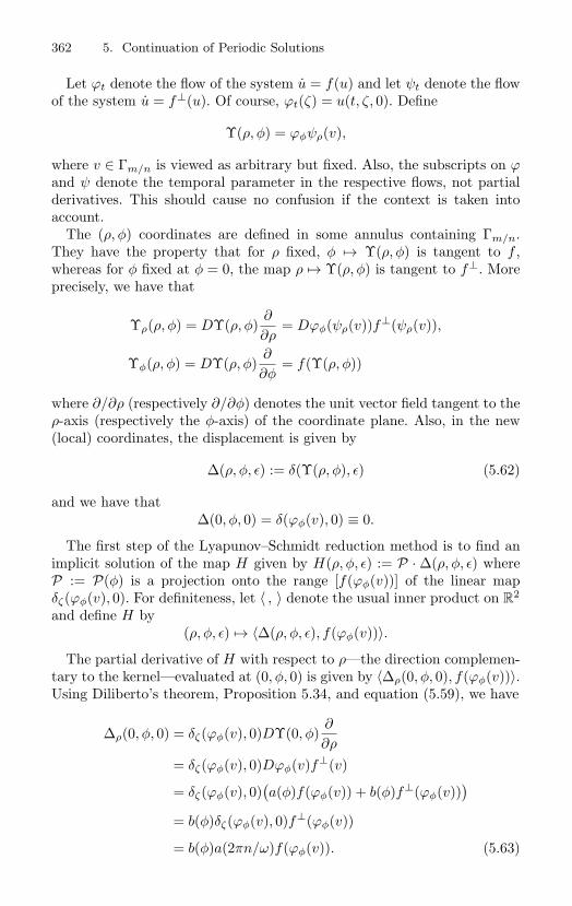
362 5. Continuation of Periodic Solutions
Let ϕt denote the flow of the system u = f(u) and let ψt denote the flowof the system u = f⊥(u). Of course, ϕt(ζ) = u(t, ζ, 0). Define
Υ(ρ, φ) = ϕφψρ(v),
where v ∈ Γm/n is viewed as arbitrary but fixed. Also, the subscripts on ϕand ψ denote the temporal parameter in the respective flows, not partialderivatives. This should cause no confusion if the context is taken intoaccount.
The (ρ, φ) coordinates are defined in some annulus containing Γm/n.They have the property that for ρ fixed, φ → Υ(ρ, φ) is tangent to f ,whereas for φ fixed at φ = 0, the map ρ → Υ(ρ, φ) is tangent to f⊥. Moreprecisely, we have that
Υρ(ρ, φ) = DΥ(ρ, φ)∂
∂ρ= Dϕφ(ψρ(v))f⊥(ψρ(v)),
Υφ(ρ, φ) = DΥ(ρ, φ)∂
∂φ= f(Υ(ρ, φ))
where ∂/∂ρ (respectively ∂/∂φ) denotes the unit vector field tangent to theρ-axis (respectively the φ-axis) of the coordinate plane. Also, in the new(local) coordinates, the displacement is given by
∆(ρ, φ, ε) := δ(Υ(ρ, φ), ε) (5.62)
and we have that∆(0, φ, 0) = δ(ϕφ(v), 0) ≡ 0.
The first step of the Lyapunov–Schmidt reduction method is to find animplicit solution of the map H given by H(ρ, φ, ε) := P · ∆(ρ, φ, ε) whereP := P(φ) is a projection onto the range [f(ϕφ(v))] of the linear mapδζ(ϕφ(v), 0). For definiteness, let 〈 , 〉 denote the usual inner product on R
2
and define H by(ρ, φ, ε) → 〈∆(ρ, φ, ε), f(ϕφ(v))〉.
The partial derivative of H with respect to ρ—the direction complemen-tary to the kernel—evaluated at (0, φ, 0) is given by 〈∆ρ(0, φ, 0), f(ϕφ(v))〉.Using Diliberto’s theorem, Proposition 5.34, and equation (5.59), we have
∆ρ(0, φ, 0) = δζ(ϕφ(v), 0)DΥ(0, φ)∂
∂ρ
= δζ(ϕφ(v), 0)Dϕφ(v)f⊥(v)
= δζ(ϕφ(v), 0)(a(φ)f(ϕφ(v)) + b(φ)f⊥(ϕφ(v))
)= b(φ)δζ(ϕφ(v), 0)f⊥(ϕφ(v))
= b(φ)a(2πn/ω)f(ϕφ(v)). (5.63)
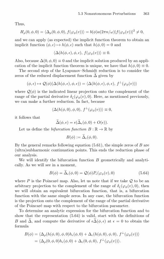
5.3 Nonautonomous Perturbations 363
Thus,
Hρ(0, φ, 0) = 〈∆ρ(0, φ, 0), f(ϕφ(v))〉 = b(φ)a(2πn/ω)|f(ϕφ(v))|2 = 0,
and we can apply (as expected) the implicit function theorem to obtain animplicit function (φ, ε) → h(φ, ε) such that h(φ, 0) = 0 and
〈∆(h(φ, ε), φ, ε), f(ϕφ(v))〉 ≡ 0.
Also, because ∆(0, φ, 0) ≡ 0 and the implicit solution produced by an appli-cation of the implicit function theorem is unique, we have that h(φ, 0) ≡ 0.
The second step of the Lyapunov–Schmidt reduction is to consider thezeros of the reduced displacement function ∆ given by
(φ, ε) → Q(φ)(∆(h(φ, ε), φ, ε)) = 〈∆(h(φ, ε), φ, ε), f⊥(ϕφ(v))〉
where Q(φ) is the indicated linear projection onto the complement of therange of the partial derivative δζ(ϕφ(v), 0). Here, as mentioned previously,we can make a further reduction. In fact, because
〈∆(h(φ, 0), φ, 0), f⊥(ϕφ(v))〉 ≡ 0,
it follows that∆(φ, ε) = ε(∆ε(φ, 0) + O(ε)).
Let us define the bifurcation function B : R → R by
B(φ) := ∆ε(φ, 0).
By the general remarks following equation (5.61), the simple zeros of B are(ultra)subharmonic continuation points. This ends the reduction phase ofour analysis.
We will identify the bifurcation function B geometrically and analyti-cally. As we will see in a moment,
B(φ) = ∆ε(φ, 0) = Q(φ)Pε(ϕφ(v), 0) (5.64)
where P is the Poincare map. Also, let us note that if we take Q to be anarbitrary projection to the complement of the range of δζ(ϕφ(v), 0), thenwe will obtain an equivalent bifurcation function, that is, a bifurcationfunction with the same simple zeros. In any case, the bifurcation functionis the projection onto the complement of the range of the partial derivativeof the Poincare map with respect to the bifurcation parameter.
To determine an analytic expression for the bifurcation function and toshow that the representation (5.64) is valid, start with the definitions ofB and ∆, and compute the derivative of ε∆(φ, ε) at ε = 0 to obtain theformula
B(φ) = 〈∆ρ(h(φ, 0), φ, 0)hε(φ, 0) + ∆ε(h(φ, 0), φ, 0), f⊥(ϕφ(v))〉= 〈∆ρ(0, φ, 0)hε(φ, 0) + ∆ε(0, φ, 0), f⊥(ϕφ(v))〉.
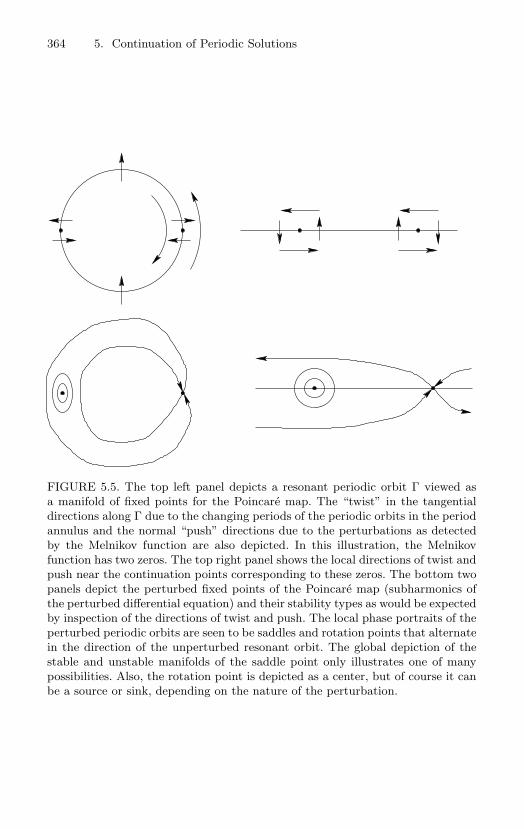
364 5. Continuation of Periodic Solutions
FIGURE 5.5. The top left panel depicts a resonant periodic orbit Γ viewed asa manifold of fixed points for the Poincare map. The “twist” in the tangentialdirections along Γ due to the changing periods of the periodic orbits in the periodannulus and the normal “push” directions due to the perturbations as detectedby the Melnikov function are also depicted. In this illustration, the Melnikovfunction has two zeros. The top right panel shows the local directions of twist andpush near the continuation points corresponding to these zeros. The bottom twopanels depict the perturbed fixed points of the Poincare map (subharmonics ofthe perturbed differential equation) and their stability types as would be expectedby inspection of the directions of twist and push. The local phase portraits of theperturbed periodic orbits are seen to be saddles and rotation points that alternatein the direction of the unperturbed resonant orbit. The global depiction of thestable and unstable manifolds of the saddle point only illustrates one of manypossibilities. Also, the rotation point is depicted as a center, but of course it canbe a source or sink, depending on the nature of the perturbation.
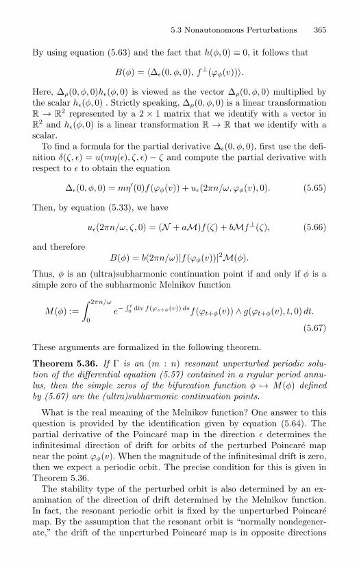
5.3 Nonautonomous Perturbations 365
By using equation (5.63) and the fact that h(φ, 0) ≡ 0, it follows that
B(φ) = 〈∆ε(0, φ, 0), f⊥(ϕφ(v))〉.
Here, ∆ρ(0, φ, 0)hε(φ, 0) is viewed as the vector ∆ρ(0, φ, 0) multiplied bythe scalar hε(φ, 0) . Strictly speaking, ∆ρ(0, φ, 0) is a linear transformationR → R
2 represented by a 2 × 1 matrix that we identify with a vector inR
2 and hε(φ, 0) is a linear transformation R → R that we identify with ascalar.
To find a formula for the partial derivative ∆ε(0, φ, 0), first use the defi-nition δ(ζ, ε) = u(mη(ε), ζ, ε) − ζ and compute the partial derivative withrespect to ε to obtain the equation
∆ε(0, φ, 0) = mη′(0)f(ϕφ(v)) + uε(2πn/ω, ϕφ(v), 0). (5.65)
Then, by equation (5.33), we have
uε(2πn/ω, ζ, 0) = (N + aM)f(ζ) + bMf⊥(ζ), (5.66)
and thereforeB(φ) = b(2πn/ω)|f(ϕφ(v))|2M(φ).
Thus, φ is an (ultra)subharmonic continuation point if and only if φ is asimple zero of the subharmonic Melnikov function
M(φ) :=∫ 2πn/ω
0e− ∫ t
0 div f(ϕs+φ(v)) dsf(ϕt+φ(v)) ∧ g(ϕt+φ(v), t, 0) dt.
(5.67)
These arguments are formalized in the following theorem.
Theorem 5.36. If Γ is an (m : n) resonant unperturbed periodic solu-tion of the differential equation (5.57) contained in a regular period annu-lus, then the simple zeros of the bifurcation function φ → M(φ) definedby (5.67) are the (ultra)subharmonic continuation points.
What is the real meaning of the Melnikov function? One answer to thisquestion is provided by the identification given by equation (5.64). Thepartial derivative of the Poincare map in the direction ε determines theinfinitesimal direction of drift for orbits of the perturbed Poincare mapnear the point ϕφ(v). When the magnitude of the infinitesimal drift is zero,then we expect a periodic orbit. The precise condition for this is given inTheorem 5.36.
The stability type of the perturbed orbit is also determined by an ex-amination of the direction of drift determined by the Melnikov function.In fact, the resonant periodic orbit is fixed by the unperturbed Poincaremap. By the assumption that the resonant orbit is “normally nondegener-ate,” the drift of the unperturbed Poincare map is in opposite directions
366 5. Continuation of Periodic Solutions
on opposite sides of the resonant orbit. The sign of the Melnikov functiondetermines the drift in the direction of the complement to the range of theinfinitesimal displacement, a direction that is known to be transverse tothe unperturbed orbit. A plot of these directions at a continuable pointsuggests the stability type as seen in Figure 5.5.
Exercise 5.37. Use the Lyapunov–Schmidt reduction to determine conditionson the triplet of functions (g1, g2, g3) so that the system of equations
1 − x2 − y2 − z2 + εg1(x, y, z) = 0,
1 − x2 − y2 − z2 + εg2(x, y, z) = 0,
xyz + εg3(x, y, z) = 0,
has solutions for small ε = 0. What (additional) condition assures that rootsfound in this way are simple?
Exercise 5.38. Consider the forced rotor given by
θ + ε sin θ = ε sin t.
The associated first order system with φ = v can be considered as a differentialequation on the cylinder R × T, where T denotes the unit circle. In this interpre-tation, all orbits of the unperturbed system are periodic. Moreover, the periodicorbit Γ corresponding to v = 0 is (1 : 1) resonant. Show that Γ is normally non-degenerate, and determine the continuation points on Γ. What can you say aboutthe (m : n) resonant periodic orbits? Change the time scale in the differentialequation to slow time τ =
√εt. What is the meaning of the continuable peri-
odic solutions relative to the transformed differential equation? The slow timeequation is a rapidly forced pendulum. Does it have subharmonics?
Exercise 5.39. Suppose that F : R3 × R → R
3 is a function given in the form
F (u, ε) = g(u) + εh(u)
where g, h : R3 → R
3 are smooth vector functions with
g(u) = (g1(u), g2(u), g3(u)), h(u) = (h1(u), h2(u), h3(u)).
Prove the following theorem: If the slot functions g1 and g2 are identical andv ∈ R
3 is such that g(v) = 0 and the vectors grad g1(v) and grad g3(v) are linearlyindependent, then there is a curve s → γ(s) in R
3 such that γ(0) = 0, γ(s) = 0,and F (γ(s), 0) ≡ 0. If such a curve exists and s = 0 is a simple zero of the scalarfunction given by s → h2(γ(s)) − h1(γ(s)), then there is a curve ε → β(ε) is R
3
such that β(0) = v and F (β(ε), ε) ≡ 0. Moreover, for each sufficiently small ε = 0,the point β(ε) is a simple zero of the function u → F (u, ε) (see [42]).
Exercise 5.40. [Multidimensional Oscillators] Suppose that the system u =f(u), for the vector case u ∈ R
n, has a T -periodic orbit Γ given by the solutiont → γ(t). Show that the number one is a Floquet multiplier of the (periodic)variational equation w = Df(γ(t))w. Prove that if the Floquet multiplier one hasalgebraic multiplicity one and if g : R
n × R × R → Rn is a smooth function given
by (u, t, ε) → g(u, t, ε) such that the corresponding map given by t → g(u, t, ε) isT -periodic for each u and ε, then Γ persists in the family u = f(u) + εg(u, t, ε).
5.3 Nonautonomous Perturbations 367
5.3.5 Limit Cycles–Entrainment–Resonance ZonesIn Section 5.3.4 we considered the continuation of (ultra)subharmonics ofthe differential equation
u = f(u) + εg(u, t, ε), u ∈ R2 (5.68)
from a resonant unperturbed periodic orbit contained in a period annulus.Here, we will consider continuation of (ultra)subharmonics from a resonantunperturbed limit cycle.
If we view the differential equation (5.68) as an autonomous first or-der system on the phase cylinder R
2 ×T, then the unperturbed differentialequation has an invariant torus Γ×T. For the theory in this section, it is notnecessary to determine the fate of the invariant torus after perturbation.However, note that if Γ is a hyperbolic limit cycle, then the correspond-ing invariant torus is a normally hyperbolic invariant manifold. Roughlyspeaking, an invariant manifold is attracting and normally hyperbolic ifthe linearized flow for each orbit on the manifold contracts normal vectorsat an exponential rate, and if the slowest such rate is faster than the fastestcontraction rate for a vector that is tangent to the manifold. There is a sim-ilar definition if the manifold is repelling or if it has both attracting andrepelling normal directions. In our case, if the limit cycle Γ is attracting,then its normal contraction rate is exponential and its tangential contrac-tion rate is zero. Moreover, the invariant unperturbed torus correspondingto Γ inherits this behavior (see Exercise 5.42). Thus, this invariant torus isnormally hyperbolic. In this case, by a powerful, important theorem (see[64] and [94]), the normally hyperbolic torus persists after perturbation.The continuation theory in this section describes the flow on this perturbedinvariant torus. Typically, there is an even number of (ultra)subharmonicsthat alternate in stability around the perturbed torus.
By the above remarks, if our unperturbed system has a resonant, at-tracting hyperbolic limit cycle, then after perturbation there is an attract-ing invariant torus and nearby perturbed orbits are attracted to stable(ultra)subharmonic orbits on this torus. In the engineering literature thisphenomenon is called entrainment: As nearby orbits are attracted to theperturbed invariant torus, their quasi-periods approach the periods of the(ultra)subharmonics on the perturbed torus. In particular, the asymptoticperiods are entrained to a multiple of the period of the input perturba-tion. For a perturbation of small amplitude, this entrained period is closeto the resonant period mη(0) as in equation (5.38). We will determine abifurcation function whose simple zeros are the continuation points of these(ultra)subharmonics.
For the remainder of this section let us consider the periodically per-turbed oscillator (5.68) under the following assumptions:(i) There is an unperturbed periodic orbit Γ in (m : n) resonance with
the periodic perturbation as in the equation (5.38).
368 5. Continuation of Periodic Solutions
(ii) There is a region R ⊆ R2 with Γ ⊂ R such that the displacement
δ : R × (−ε0, ε0) → R2 is defined for some ε0 > 0.
(iii) As in Proposition 5.34, the periodic orbit Γ is a hyperbolic limit cycle,or alternatively, the differential of the return time map σ → T (σ, 0)at v = Γ∩Σ defined on some curve Σ transverse to Γ, is nonsingular.
Let us also note that by the third hypothesis and Proposition 5.34, we havethat Kernel δζ(ζ, 0) = [f(ζ)] for ζ ∈ Γ, and therefore the invariant torusΓ × T is normally nondegenerate.
The analysis required to obtain the bifurcation function in case the un-perturbed resonant periodic orbit is a limit cycle is analogous to the analysiscarried out in the last section for the case of a regular period annulus. Inparticular, using the same notation as before, we can apply the Lyapunov–Schmidt reduction to the displacement function represented in the same(ρ, φ)-coordinates.
By the abstract theory of the Lyapunov–Schmidt reduction, ρ can be de-fined implicitly as a function of (φ, ε) when it is projected onto the range ofthe infinitesimal displacement, that is, the partial derivative of the displace-ment with respect to the space variable. However, it is easy and instructiveto verify this directly. In fact, with respect to the (ρ, φ)-coordinates, thesection Σ as in Proposition 5.34 is just an integral curve of f⊥, and henceit is orthogonal to Γ. Thus, let us first consider the map
(ρ, φ, ε) → 〈∆(ρ, φ, ε), r1f(ϕφ(v)) + r2f⊥(ϕφ(v))〉
where r1 and r2 are defined in Proposition 5.34 and ∆ is the local co-ordinate representation defined in display (5.62) of the displacement. Byequation (5.63) and this proposition, its differential with respect to ρ at(ρ, ε) = (0, 0) is given by
〈∆ρ(0, φ, 0), r1f(ϕφ(v)) + r2f⊥(ϕφ(v))〉
= 〈δζ(ϕφ(v), 0)DΥ(0, φ)∂/∂ρ, r1f(ϕφ(v)) + r2f⊥(ϕφ(v))〉
= 〈b(φ)δζ(ϕφ(v), 0)f⊥(ϕφ(v)), r1f(ϕφ(v)) + r2f⊥(ϕφ(v))〉
= b(φ)〈r1f(ϕφ(v)) + r2f⊥(ϕφ(v)), r1f(ϕφ(v)) + r2f
⊥(ϕφ(v))〉= b(φ)|f(ϕφ(v))|2(r2
1 + r22).
Also, let us note that during the course of the last computation we haveproved that
∆ρ(0, φ, 0) = b(φ)(r1f(ϕφ(v)) + r2f⊥(ϕφ(v))). (5.69)
By the assumptions for this section, we have r21 + r2
2 = 0, and therefore∆ρ(0, φ, 0) = 0. Thus, by an application of the implicit function theorem,there is a function (φ, ε) → h(φ, ε) such that h(φ, 0) ≡ 0 and
〈∆(h(φ, ε), φ, ε), r1f(ϕφ(v)) + r2f⊥(ϕφ(v))〉 ≡ 0.
5.3 Nonautonomous Perturbations 369
Recall that Γ × T is normally nondegenerate if
Kernel δζ(ϕφ(v), 0) = [f(φφ(v))].
Since this kernel is a one-dimensional subspace of the two-dimensional tan-gent space of the Poincare section, the range of the infinitesimal displace-ment must also be one-dimensional, and therefore r2
1 + r22 = 0. Of course,
this inequality also holds if either Γ is hyperbolic or the differential of thereturn time is nonzero.
The reduced displacement function is just the projection of the dis-placement onto a complement for the range of the infinitesimal displace-ment. For definiteness, let us consider the reduced displacement function(φ, ε) → ∆(φ, ε) given by
∆(φ, ε) = 〈∆(h(φ, ε), φ, ε), −r2f(ϕφ(v)) + r1f⊥(ϕφ(v))〉.
Since ∆(h(φ, 0), φ, 0) ≡ 0, we have ∆(φ, 0) ≡ 0 and
∆(φ, ε) = ε(∆ε(φ, 0) + O(ε)).
If the bifurcation function B : R → R is defined by B(φ) := ∆ε(φ, 0), thenwe have, as usual, the following proposition: The simple zeros of B are the(ultra)subharmonic continuation points. This ends the reduction step.
The identification of the bifurcation function B is accomplished with theaid of a simple computation. Indeed, using the definition of B, we havethat
B(φ) = 〈∆ρ(h(φ, 0), φ, 0)hε(φ, 0) + ∆ε(h(φ, 0), φ, 0),− r2f(ϕφ(v)) + r1f
⊥(ϕφ(v))〉. (5.70)
To simplify this expression, apply identity (5.69) to obtain the representa-tion
B(φ) = 〈∆ε(h(φ, 0), φ, 0), −r2f(ϕφ(v)) + r1f⊥(ϕφ(v))〉.
Also, let us note that, as in the last section, B(φ) = Q(φ)Pε(ϕφ(v), 0).Using the equations (5.65) and (5.37), substitute the solution (5.33) of
the nonhomogeneous variational equation for ∆ε to obtain the formula
B(φ) = 〈mη′(0)f(ϕφ(v)) +(N (φ) + a(2πn/ω)M(φ)
)f(ϕφ(v))
+ b(2πn/ω)M(φ)f⊥(ϕφ(v)),−r2f(ϕφ(v)) + r1f⊥(ϕφ(v))〉
where, by Proposition 5.34,
r1 = a(2πn/ω, ϕφ(v)), r2 = b(2πn/ω, ϕφ(v)) − 1.
Hence, the bifurcation function is given by
B(φ) =((1 − b(2πn/ω, ϕφ(v)))(mk + N (φ))
+ a(2πn/ω, ϕφ(v))M(φ))|f(ϕφ(v))|2.
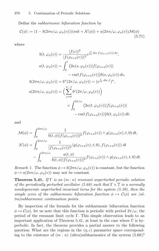
370 5. Continuation of Periodic Solutions
Define the subharmonic bifurcation function by
C(φ) := (1 − b(2πn/ω, ϕφ(v)))(mk + N (φ)) + a(2πn/ω, ϕφ(v))M(φ)(5.71)
where
b(t, ϕφ(v)) =|f(v)|2
|f(ϕt+φ(v))|2 e∫ t0 div f(ϕs+φ(v)) ds,
a(t, ϕφ(v)) =∫ t
0
(2κ(s, ϕφ(v))|f(ϕs+φ(v))|
− curl f(ϕs+φ(v)))b(s, ϕφ(v)) ds,
b(2πn/ω, ϕφ(v)) = bn(2π/ω, ϕφ(v)) = (e∫Γ div f )n,
a(2πn/ω, ϕφ(v)) =( n−1∑
j=0
bj(2π/ω, ϕφ(v)))
×∫ 2π/ω
0
(2κ(t, ϕφ(v))|f(ϕt+φ(v))|
− curl f(ϕt+φ(v)))b(t, ϕφ(v)) dt;
and
M(φ) =∫ 2πn/ω
0
1b(t, φ)|f(ϕt+φ(v))|2 f(ϕt+φ(v)) ∧ g(ϕt+φ(v), t, 0) dt,
N (φ) =∫ 2πn/ω
0
1|f(ϕt+φ(v))|2 〈g(ϕt+φ(v), t, 0), f(ϕt+φ(v))〉 dt
−∫ 2πn/ω
0
a(t, φ)b(t, φ)|f(ϕt+φ(v))|2 f(ϕt+φ(v)) ∧ g(ϕt+φ(v), t, 0) dt.
Remark 1. The function φ → b(2πn/ω, ϕφ(v)) is constant, but the functionφ → a(2πn/ω, ϕφ(v)) may not be constant.
Theorem 5.41. If Γ is an (m : n) resonant unperturbed periodic solutionof the periodically perturbed oscillator (5.68) such that Γ× T is a normallynondegenerate unperturbed invariant torus for the system (5.39), then thesimple zeros of the subharmonic bifurcation function φ → C(φ) are (ul-tra)subharmonic continuation points.
By inspection of the formula for the subharmonic bifurcation functionφ → C(φ), let us note that this function is periodic with period 2π/ω, theperiod of the resonant limit cycle Γ. This simple observation leads to animportant application of Theorem 5.41, at least in the case where Γ is hy-perbolic. In fact, the theorem provides a partial answer to the followingquestion: What are the regions in the (η, ε) parameter space correspond-ing to the existence of (m : n) (ultra)subharmonics of the system (5.68)?
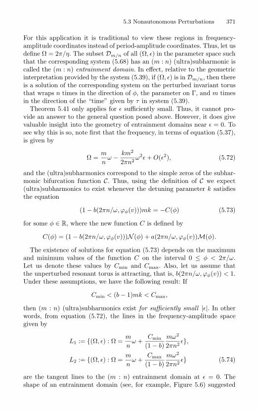
5.3 Nonautonomous Perturbations 371
For this application it is traditional to view these regions in frequency-amplitude coordinates instead of period-amplitude coordinates. Thus, let usdefine Ω = 2π/η. The subset Dm/n of all (Ω, ε) in the parameter space suchthat the corresponding system (5.68) has an (m : n) (ultra)subharmonic iscalled the (m : n) entrainment domain. In effect, relative to the geometricinterpretation provided by the system (5.39), if (Ω, ε) is in Dm/n, then thereis a solution of the corresponding system on the perturbed invariant torusthat wraps n times in the direction of φ, the parameter on Γ, and m timesin the direction of the “time” given by τ in system (5.39).
Theorem 5.41 only applies for ε sufficiently small. Thus, it cannot pro-vide an answer to the general question posed above. However, it does givevaluable insight into the geometry of entrainment domains near ε = 0. Tosee why this is so, note first that the frequency, in terms of equation (5.37),is given by
Ω =m
nω − km2
2πn2 ω2ε + O(ε2), (5.72)
and the (ultra)subharmonics correspond to the simple zeros of the subhar-monic bifurcation function C. Thus, using the definition of C we expect(ultra)subharmonics to exist whenever the detuning parameter k satisfiesthe equation
(1 − b(2πn/ω, ϕφ(v)))mk = −C(φ) (5.73)
for some φ ∈ R, where the new function C is defined by
C(φ) = (1 − b(2πn/ω, ϕφ(v)))N (φ) + a(2πn/ω, ϕφ(v))M(φ).
The existence of solutions for equation (5.73) depends on the maximumand minimum values of the function C on the interval 0 ≤ φ < 2π/ω.Let us denote these values by Cmin and Cmax. Also, let us assume thatthe unperturbed resonant torus is attracting, that is, b(2πn/ω, ϕφ(v)) < 1.Under these assumptions, we have the following result: If
Cmin < (b − 1)mk < Cmax,
then (m : n) (ultra)subharmonics exist for sufficiently small |ε|. In otherwords, from equation (5.72), the lines in the frequency-amplitude spacegiven by
L1 := (Ω, ε) : Ω =m
nω +
Cmin
(1 − b)mω2
2πn2 ε,
L2 := (Ω, ε) : Ω =m
nω +
Cmax
(1 − b)mω2
2πn2 ε (5.74)
are the tangent lines to the (m : n) entrainment domain at ε = 0. Theshape of an entrainment domain (see, for example, Figure 5.6) suggested
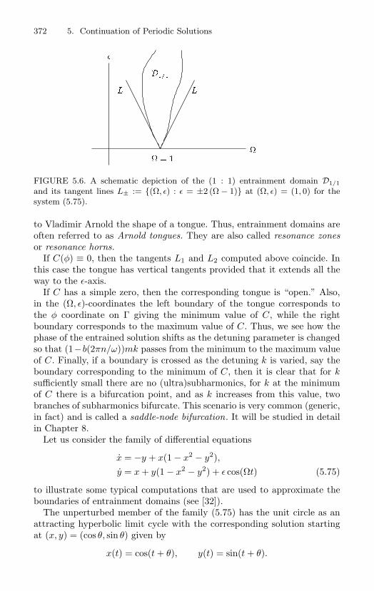
372 5. Continuation of Periodic Solutions
LL
D
FIGURE 5.6. A schematic depiction of the (1 : 1) entrainment domain D1/1
and its tangent lines L± := (Ω, ε) : ε = ±2 (Ω − 1) at (Ω, ε) = (1, 0) for thesystem (5.75).
to Vladimir Arnold the shape of a tongue. Thus, entrainment domains areoften referred to as Arnold tongues. They are also called resonance zonesor resonance horns.
If C(φ) ≡ 0, then the tangents L1 and L2 computed above coincide. Inthis case the tongue has vertical tangents provided that it extends all theway to the ε-axis.
If C has a simple zero, then the corresponding tongue is “open.” Also,in the (Ω, ε)-coordinates the left boundary of the tongue corresponds tothe φ coordinate on Γ giving the minimum value of C, while the rightboundary corresponds to the maximum value of C. Thus, we see how thephase of the entrained solution shifts as the detuning parameter is changedso that (1−b(2πn/ω))mk passes from the minimum to the maximum valueof C. Finally, if a boundary is crossed as the detuning k is varied, say theboundary corresponding to the minimum of C, then it is clear that for ksufficiently small there are no (ultra)subharmonics, for k at the minimumof C there is a bifurcation point, and as k increases from this value, twobranches of subharmonics bifurcate. This scenario is very common (generic,in fact) and is called a saddle-node bifurcation. It will be studied in detailin Chapter 8.
Let us consider the family of differential equations
x = −y + x(1 − x2 − y2),y = x + y(1 − x2 − y2) + ε cos(Ωt) (5.75)
to illustrate some typical computations that are used to approximate theboundaries of entrainment domains (see [32]).
The unperturbed member of the family (5.75) has the unit circle as anattracting hyperbolic limit cycle with the corresponding solution startingat (x, y) = (cos θ, sin θ) given by
x(t) = cos(t + θ), y(t) = sin(t + θ).
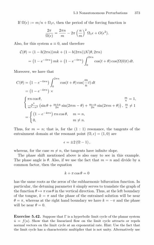
5.3 Nonautonomous Perturbations 373
If Ω(ε) := m/n + Ω1ε, then the period of the forcing function is
2π
Ω(ε)=
2πn
m− 2π
( n
m
)2Ω1ε + O(ε2).
Also, for this system a ≡ 0, and therefore
C(θ) = (1 − b(2πn))mk + (1 − b(2πn))N (θ, 2πn)
=(1 − e−4πn
)mk +
(1 − e−4πn
) ∫ 2πn
0cos(t + θ) cos(Ω(0)t) dt.
Moreover, we have that
C(θ) =(1 − e−4πn
) ∫ 2πn
0cos(t + θ) cos(
m
nt) dt
=(1 − e−4πn
)×
πn cos θ, mn = 1,
n2
m2−n2
(sin θ + m+n
2n sin(2πm − θ) + m−n2n sin(2πm + θ)
), m
n = 1
=
(1 − e−4πn
)πn cos θ, m = n,
0, m = n.
Thus, for m = n; that is, for the (1 : 1) resonance, the tangents of theentrainment domain at the resonant point (Ω, ε) = (1, 0) are
ε = ±2 (Ω − 1) ,
whereas, for the case m = n, the tangents have infinite slope.The phase shift mentioned above is also easy to see in this example.
The phase angle is θ. Also, if we use the fact that m = n and divide by acommon factor, then the equation
k + π cos θ = 0
has the same roots as the zeros of the subharmonic bifurcation function. Inparticular, the detuning parameter k simply serves to translate the graph ofthe function θ → π cos θ in the vertical direction. Thus, at the left boundaryof the tongue, k = π and the phase of the entrained solution will be nearθ = π, whereas at the right hand boundary we have k = −π and the phasewill be near θ = 0.
Exercise 5.42. Suppose that Γ is a hyperbolic limit cycle of the planar systemu = f(u). Show that the linearized flow on the limit cycle attracts or repelsnormal vectors on the limit cycle at an exponential rate. Hint: Use the fact thatthe limit cycle has a characteristic multiplier that is not unity. Alternatively use
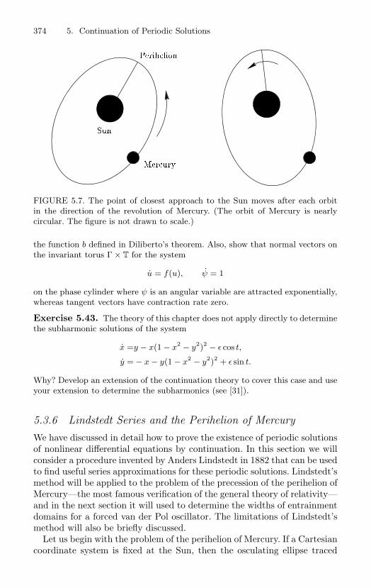
374 5. Continuation of Periodic Solutions
Mercury
Perihelion
Sun
FIGURE 5.7. The point of closest approach to the Sun moves after each orbitin the direction of the revolution of Mercury. (The orbit of Mercury is nearlycircular. The figure is not drawn to scale.)
the function b defined in Diliberto’s theorem. Also, show that normal vectors onthe invariant torus Γ × T for the system
u = f(u), ψ = 1
on the phase cylinder where ψ is an angular variable are attracted exponentially,whereas tangent vectors have contraction rate zero.
Exercise 5.43. The theory of this chapter does not apply directly to determinethe subharmonic solutions of the system
x =y − x(1 − x2 − y2)2 − ε cos t,
y = − x − y(1 − x2 − y2)2 + ε sin t.
Why? Develop an extension of the continuation theory to cover this case and useyour extension to determine the subharmonics (see [31]).
5.3.6 Lindstedt Series and the Perihelion of MercuryWe have discussed in detail how to prove the existence of periodic solutionsof nonlinear differential equations by continuation. In this section we willconsider a procedure invented by Anders Lindstedt in 1882 that can be usedto find useful series approximations for these periodic solutions. Lindstedt’smethod will be applied to the problem of the precession of the perihelion ofMercury—the most famous verification of the general theory of relativity—and in the next section it will used to determine the widths of entrainmentdomains for a forced van der Pol oscillator. The limitations of Lindstedt’smethod will also be briefly discussed.
Let us begin with the problem of the perihelion of Mercury. If a Cartesiancoordinate system is fixed at the Sun, then the osculating ellipse traced
5.3 Nonautonomous Perturbations 375
out by the motion of Mercury is observed to precess. This means thatthe perihelion of Mercury—the point of closest approach to the Sun—changes after each revolution, moving in the direction of the motion ofthe planet (see Figure 5.7). In fact, the point of perihelion is observed toadvance by approximately 43 seconds of arc per century. No satisfactoryexplanation of this phenomenon was known until after the introduction ofthe general theory of relativity by Albert Einstein. In particular, in 1915Einstein found that his theory indeed predicts a precession of 43 secondsof arc per century—a stunning confirmation of his theory (see [168, PartI]). Shortly thereafter, Karl Schwarzschild (1916) found a solution of thegravitational field equations for a circularly symmetric body—the Sun—and he gave a rigorous derivation of the same relativistic correction to theNewtonian solution for the orbit of Mercury (see, for example, [183, p. 247]for more history).
While the derivation of Schwarzschild’s solution of the perihelion prob-lem from the general theory of relativity is beyond the scope of this book(see [104], [168], or [183] for readable accounts), it turns out that the recip-rocal ρ of the distance r from the center of the Sun to Mercury, as Mercurymoves on a “geodesic” with respect to the “space-time metric” produced bythe Sun, is closely approximated by a solution of the differential equation
d2ρ
dφ2 =1β2 − ρ + αρ2 (5.76)
where
β2 =M2
G0m1m22, α =
3G0m1
c2 ,
M is the magnitude of the angular momentum, m1 is the mass of the Sun,m2 is the mass of Mercury, G0 is the gravitational constant, and c is thespeed of light [104]. We will predict the precession of the perihelion ofMercury from the differential equation (5.76).
In view of the results in Section 3.2.2, especially the harmonic oscillatormodel (3.22) for Kepler motion, the system (5.76) with α = 0 is exactlythe same as the model predicted from Newton’s theory. In fact, as we haveseen, this model predicts a fixed elliptical orbit for Mercury. We will seethat the perturbed orbit precesses.
The sizes of the parameters in equation (5.76) depend on the choice ofthe units of measurement. Thus, it is not meaningful to say that α is a smallparameter. This basic problem is ubiquitous in applied mathematics. Whilemost authors do not worry about the units, there is only one correct wayto proceed: rescale the variables so that the new system is dimensionless.For equation (5.76), if we define a new dependent variable η := β2ρ, thenthe differential equation is recast in the form
d2η
dφ2 + η = 1 + εη2 (5.77)
376 5. Continuation of Periodic Solutions
where the ratio ε := α/β2 is dimensionless. To evaluate ε, use Exercise 3.10to find an expression for the angular momentum M of Mercury, and thenuse the physical constants
G0 = 6.668 × 10⁻¹¹ m3
kg·sec2 , a = (387)(149, 598, 845)m,
c = 3 × 10⁸ msec , mSun = (332700)(5.977) × 1024kg,
e = 0.206,
(5.78)
reported for example in [72] to compute the approximation
ε ≈ 7.973 × 10⁻⁸. (5.79)
The differential equation (5.77) has two rest points in the phase plane:a center near the point with coordinates (1, 0), and a saddle near (1/ε, 0).Moreover, the orbit corresponding to the perturbed motion of Mercurycorresponds to one of the periodic orbits surrounding the center (see Exer-cise 5.44).
Exercise 5.44. Show that the phase portrait of the system (5.77) has exactlytwo rest points: a saddle and a sink; approximate the positions of these restpoints with power series in ε; and show that the orbit of Mercury correspondsto a periodic orbit. Note that it is not enough for this physical problem to provethe result for “sufficiently small epsilon.” Rather, the value ε = α/β2 must beused! Hint: Initial conditions for the orbit of Mercury can be approximated fromthe physical data. The level sets of the “energy” corresponding to the differentialequation (5.77) are invariant manifolds in the phase plane. In fact, one of themforms the boundary of the period annulus.
How can we find a useful approximation of the perturbed periodic orbitcorresponding to the motion of Mercury? To answer this question, let usview ε as a parameter and observe that the differential equation (5.77) isanalytic. Thus, the periodic solution φ → η(φ, ε) that we wish to approxi-mate is given by an analytic function η of two variables. Also, this solutionis an analytic function of the initial conditions. Thus, the perturbed solu-tion can be expanded as a convergent power series in ε; at least this is trueif ε is sufficiently small. We will come back to this problem in a moment.For now, let us assume that there is a series expansion of the form
η(φ, ε) = η0(φ) + η1(φ)ε + η2(φ)ε2 + O(ε3). (5.80)
A natural idea is to substitute the series (5.80) into the differential equa-tion (5.77), and then try to solve for the unknown Taylor coefficients byequating like powers of ε. In fact, if this is done, then (using dots to denotederivatives with respect to φ) the order zero equation is
η0 + η0 = 1. (5.81)
5.3 Nonautonomous Perturbations 377
Note that we have some freedom in the choice of initial data for thesolution of the differential equation (5.81). For example, if we consider thesystem in the phase plane, then there is an interval on the η-axis that liesto the right of the unperturbed rest point at (1, 0) and contains one of theintersection points of our perturbed periodic orbit with the η-axis. In fact,this interval can be chosen to be a Poincare section. Thus, we can supposethat the desired periodic orbit corresponding to the solution φ → η(φ, ε)starts at φ = 0 on this section at a point with coordinate 1 + b for someb = b(ε) > 0. In other words, for sufficiently small ε > 0, we have the initialconditions η(0, ε) = 1 + b and η(0, ε) = 0. In particular, η0(0) = 1 + b,η0(0) = 0, and the corresponding solution or the order zero differentialequation is
η0(φ) = 1 + b cos φ.
Note that truncation at this order predicts elliptical motion for Mercury.In fact, the zero order approximation is just the solution of the harmonicoscillator model (3.22) of Kepler motion.
By using a trigonometric identity and some algebraic manipulation, thefirst order term in the series expansion of η is seen to be the solution of theinitial value problem
η1 + η1 =( 1β2 +
b2
2)
+2b
β2 cos φ +b2
2cos 2φ,
η1(0) = 0, η1(0) = 0, (5.82)
and, by an application of the variation of constants formula, the solutionof this initial value problem has the form
η1(φ) = c1 + c2φ sin φ + c3 cos 2φ
where c1, c2, and c3 are nonzero constants.We now have a problem: The first order approximation
η(φ) ≈ η0(φ) + εη1(φ)
is not periodic. Indeed, because one Fourier mode of the forcing function inthe differential equation (5.82) is in resonance with the natural frequency ofthe harmonic oscillator, the expression for η1(φ) contains the secular termc2φ sin φ. Indeed, the function φ → c2φ sin φ is unbounded as φ → ∞.
The word “secular” means an event that occurs once in a century. Theinference is clear: Even if its coefficient is small, a secular term will eventu-ally have arbitrarily large values. In particular, if there is a secular term inan approximation with a finite number of terms, then the approximationwill not be periodic unless there is a fortuitous cancellation.
We started with a periodic function φ → η(φ, ε), but the first order termin its series expansion in powers of the perturbation parameter ε is notperiodic. How can this be?
378 5. Continuation of Periodic Solutions
As an example to illustrate the reason for the appearance of secularterms, let us consider the harmonic oscillator with small detuning given by
u + (1 + ε)2u = 0
with the initial conditions u(0) = b and u(0) = 0. For this example, wehave that
u(t, ε) = b cos((1 + ε)t) = b cos t − (bt sin t)ε − 12(bt2 cos t)ε2 + O(ε3).
Hence, even though the series represents a periodic function, every finiteorder approximation obtained by truncation of the series is unbounded.Clearly, these finite order approximations are not useful over long time in-tervals. Also, note that the terms in this series expansion have the “wrong”period. Whereas the solution is periodic with period 2π/(1+ε), the trigono-metric terms on the right hand side all have period 2π.
Lindstedt observed that secular terms appear in the series for a perturbedperiodic solution because the parameter-dependent frequency of the per-turbed periodic orbit is not taken into account. He showed that the secularterms can be eliminated if the solution and its frequency are simultaneouslyexpanded in powers of the perturbation parameter.
As an illustration of Lindstedt’s method, let us consider a perturbedlinear system of the form
u + λ2u = εf(u, u, ε) (5.83)
that has a family of periodic solutions t → u(t, ε) with the initial conditionsu(0, ε) = b and u(0, ε) = 0. In other words, the corresponding periodic orbitsin the phase plane all pass through the point with coordinates (b, 0). Also,let us define the function ω given by ε → ω(ε) such that the frequency ofthe periodic solution t → u(t, ε) is ω(ε).
Lindstedt introduces a new independent variable
τ = ω(ε)t
so that the desired periodic solution t → u(t, ε) is given by
u(t, ε) = v(ω(ε)t, ε)
where τ → v(τ, ε) is the 2π-periodic solution of the initial value problem
ω2(ε)v′′ + λ2v = εf(v, ω(ε)v′, ε), v(0, ε) = b, v′(0, ε) = 0 (5.84)
and v′ denotes the derivative of v with respect to τ .Lindstedt’s computational method is the following: Write the 2π-periodic
function τ → v(τ, ε) and the frequency ε → ω(ε) as series
v(τ, ε) = v0(τ) + v1(τ)ε + v2(τ)ε2 + · · · ,
ω(ε) = λ + ω1ε + ω2ε2 + · · · ,
5.3 Nonautonomous Perturbations 379
substitute these series into the differential equation (5.84), and then com-pute the unknown coefficients recursively by equating the terms with likepowers of ε. Alternatively, the differential equations for the Taylor coeffi-cients of v can be computed directly from the differential equation (5.84)as variational equations.
To determine the order zero coefficient, set ε = 0 in equation (5.84) tosee that v0 is the solution of the initial value problem
λ2(w′′ + w) = 0, w(0) = b, w′(0) = 0,
and therefore
v0(τ) = b cos τ. (5.85)
Next, let us note that v1(τ) = vε(τ, 0). Hence, by differentiating bothsides of equation (5.84) with respect to ε and evaluating at ε = 0, thefunction v1 is seen to be the solution of the initial value problem
λ2(w′′ + w) = f(b cos τ, −λb sin τ, 0) + 2λω1b cos τ,
w(0) = 0, w′(0) = 0. (5.86)
Because the function τ → v(τ, ε) is 2π-periodic independent of ε, so is thefunction τ → vε(τ, 0), and therefore the point (b, 0) is a continuation pointof periodic solutions in the phase plane for the (usual) first order systemcorresponding to the differential equation in display (5.86). By rescalingand then applying Theorem 5.1 to this first order system, it follows that∫ 2π
0(f(b cos τ, −λb sin τ, 0) + 2λω1b cos τ) sin τ dτ = 0.
Hence, the Fourier series for the function τ → f(b cos τ, −λb sin τ, 0), whichhas the form
A0 + A1 cos τ + B1 sin τ +∞∑
n=2
(An cos nτ + Bn sin nτ),
must be such that B1 = 0. If we impose this condition and also chooseω1 = A1/(2λb), then the forcing function on the right hand side of thelinear system (5.86) has no resonant term. Thus, the corresponding solutionv1 contains no secular terms, and it is periodic with period 2π.
Using the second order variational equation, Theorem 5.1, and an appro-priate choice of ω2, all secular terms can be eliminated in the correspondinglinear system, and the function v2 is therefore periodic with period 2π. Infact, this procedure can be repeated to determine all of the coefficientsof the Taylor series in ε for the perturbed frequency ω(ε) and the solu-tion v. Moreover, it follows from our assumptions that the resulting seriesconverge.
380 5. Continuation of Periodic Solutions
The original periodic solution is represented by a series of form
u(t, ε) = v(ω(ε)t, ε) = b cos(ω(ε)t) + v1(ω(ε)t)ε + O(ε2) (5.87)
where v1 is determined above, and the frequency of the original periodicsolution is given by
ω(ε) = λ +A1
2λbε + O(ε).
However, let us note that because the series coefficients of the series (5.87)depend on ε, the Lindstedt series expansion for u is not a Taylor series.
If the Lindstedt procedure is carried out to some finite order—the onlypossibility in most applied problems—then, to obtain an approximation tothe desired periodic solution, we must substitute a truncation of the seriesfor the frequency ω into a truncation of the Lindstedt series for the periodicsolution. This leads to the question “How well does the truncated Lindstedtseries approximate the original periodic solution?” The answer for the caseconsidered here is that the difference between the nth order truncation andthe solution is O(εn+1) on a time interval of length C/ε for some constantC > 0. See [130] for a careful treatment of order estimates of this type.
The error estimate just mentioned for Lindstedt series for the case of aone-dimensional oscillator can be obtained from the associated Taylor se-ries for the same solution. However, the analysis is much more complicatedfor multidimensional differential equations. For example, for Hamiltonianperturbations of multidimensional Hamiltonian systems, the Lindstedt se-ries generally diverge! This famous result of Poincare is very important inthe history of mathematics. The divergence of these series suggests that theunderlying dynamics must be very complex. In fact, this observation ledPoincare to several major results, for example, the discovery of chaotic dy-namics in Hamiltonian dynamical systems (see [10], [17], [56], [113], [110],[123], [127], [128], and [168]). On the other hand, Lindstedt series are usefulfor approximating the periodic solutions that are obtained as continuationsof periodic orbits of the type considered in this chapter. In fact, it is noaccident that Theorem 5.1 is used to obtain the Lindstedt series for theexample analyzed above. The bifurcation functions (called the determiningequations in the context of Lindstedt series) can be used to obtain Lindst-edt approximations for the continued periodic solutions in each case thatwe have discussed (see Exercise 5.46).
Let us return to the perihelion of Mercury.To apply Lindstedt series to obtain an approximation for the precession
of perihelion, introduce new variables
v := η − 1, τ = ω(ε)φ
into equation (5.77) so that
ω2(ε)v′′ + v = ε(1 + v)2
5.3 Nonautonomous Perturbations 381
(where v′ denotes dv/dτ), and use equations (5.85) and (5.86) to show thatv0(τ) = b cos τ and v1 is the solution of the initial value problem
w′′ + w =(1 +
b2
2)
+ 2b(1 + ω1) cos τ +b2
2cos 2τ
with initial conditions w(0) = w′(0) = 0. Thus, following Lindstedt’s pro-cedure, if ω1 := −1, then the secular terms are eliminated. In fact, if werevert to the original variables, then we have
ρ(φ) =1β2 +
b
β2 cos((1 − α/β2)φ
)+ O(ε) (5.88)
where ε = α/β2. Moreover, the lowest order truncation of the Lindstedtseries (5.88) that includes the relativistic correction yields the approxima-tion
ρ(φ) ≈ 1β2 +
b
β2 cos((1 − α/β2)φ
). (5.89)
In view of equation (5.89), the distance r = 1/ρ of Mercury to the centerof the Sun is approximated by
r ≈ β2
1 + b cos((1 − α/β2)φ
) . (5.90)
Also, the perihelion for this elliptical orbit occurs when the argument of thecosine is a multiple of 2π. Thus, if the orbit starts at perihelion at φ = 0,then after one revolution it returns to perihelion when (1 − α/β2)φ = 2π,that is, when φ has advanced by approximately 2πα/β2 radians from theunperturbed value φ = 2π.
Using the expression for Kepler’s third law in Exercise 3.10 and thephysical constants (5.78), the orbital period of Mercury is seen to be
T ≈ 7.596 × 10⁶sec.
In other words, Mercury orbits the Sun approximately 414.9 times in acentury. Using the estimate for α/β2 in display (5.79), the orbital advanceof the perihelion per century is thus found to be 2.08×10⁻⁴ radians, or ap-proximately 43 seconds of arc per century. (Can you imagine how Einsteinmust have felt when he computed this number?)
Exercise 5.45. For the perturbed harmonic oscillator u + u = εu, the naturalfrequency is “corrected” at first order in the perturbation parameter by ω(ε) =1 − ε. What is the first order correction if the perturbation is εu2 or εu3? Whatabout εun.
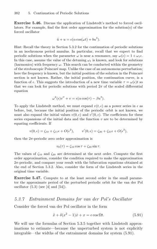
382 5. Continuation of Periodic Solutions
Exercise 5.46. Discuss the application of Lindstedt’s method to forced oscil-lators. For example, find the first order approximation for the solution(s) of theforced oscillator
u + u = ε(α cos(ωt) + bu3).
Hint: Recall the theory in Section 5.3.2 for the continuation of periodic solutionsin an isochronous period annulus. In particular, recall that we expect to findperiodic solutions when the parameter ω is near a resonance, say ω(ε) = 1 + ω1ε.In this case, assume the value of the detuning ω1 is known, and look for solutions(harmonics) with frequency ω. This search can be conducted within the geometryof the stroboscopic Poincare map. Unlike the case of an autonomous perturbation;here the frequency is known, but the initial position of the solution in the Poincaresection is not known. Rather, the initial position, the continuation curve, is afunction of ε. This suggests the introduction of a new time variable τ = ω(ε)t sothat we can look for periodic solutions with period 2π of the scaled differentialequation
ω2(ε)v′′ + v = ε(α cos(τ) − βu3).
To apply the Lindstedt method, we must expand v(t, ε) as a power series in ε asbefore, but, because the initial position of the periodic orbit is not known, wemust also expand the initial values v(0, ε) and v′(0, ε). The coefficients for theseseries expansions of the initial data and the function v are to be determined byequating coefficients. If
v(0, ε) = ζ10 + ζ11ε + O(ε2), v′(0, ε) = ζ20 + ζ21ε + O(ε2),
then the 2π-periodic zero order approximation is
v0(τ) = ζ10 cos τ + ζ20 sin τ.
The values of ζ10 and ζ20 are determined at the next order. Compute the firstorder approximation, consider the condition required to make the approximation2π-periodic, and compare your result with the bifurcation equations obtained atthe end of Section 5.3.2. Also, consider the form of the Lindstedt series in theoriginal time variable.
Exercise 5.47. Compute to at the least second order in the small parame-ter the approximate period of the perturbed periodic orbit for the van der Poloscillator (5.3) (see [4] and [54]).
5.3.7 Entrainment Domains for van der Pol’s OscillatorConsider the forced van der Pol oscillator in the form
x + δ(x2 − 1)x + x = ε cos Ωt. (5.91)
We will use the formulas of Section 5.3.5 together with Lindstedt approx-imations to estimate—because the unperturbed system is not explicitlyintegrable—the widths of the entrainment domains for system (5.91).
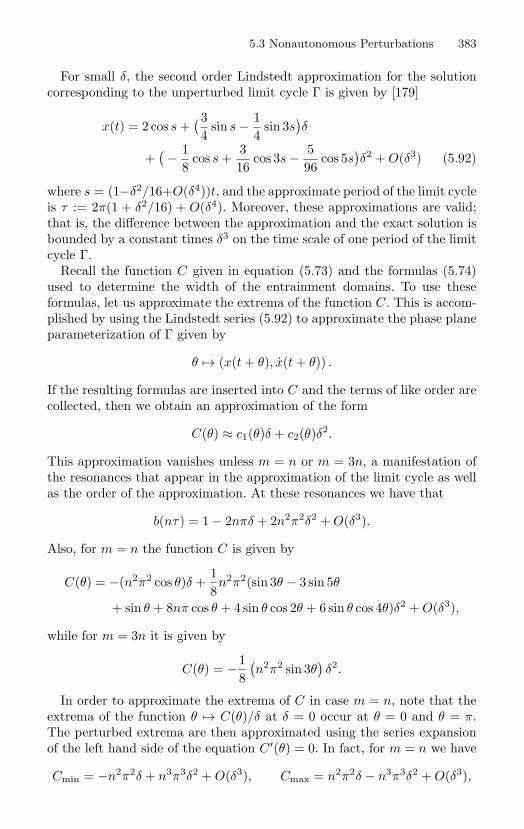
5.3 Nonautonomous Perturbations 383
For small δ, the second order Lindstedt approximation for the solutioncorresponding to the unperturbed limit cycle Γ is given by [179]
x(t) = 2 cos s +(34
sin s − 14
sin 3s)δ
+(
− 18
cos s +316
cos 3s − 596
cos 5s)δ2 + O(δ3) (5.92)
where s = (1−δ2/16+O(δ4))t, and the approximate period of the limit cycleis τ := 2π(1 + δ2/16) + O(δ4). Moreover, these approximations are valid;that is, the difference between the approximation and the exact solution isbounded by a constant times δ3 on the time scale of one period of the limitcycle Γ.
Recall the function C given in equation (5.73) and the formulas (5.74)used to determine the width of the entrainment domains. To use theseformulas, let us approximate the extrema of the function C. This is accom-plished by using the Lindstedt series (5.92) to approximate the phase planeparameterization of Γ given by
θ → (x(t + θ), x(t + θ)) .
If the resulting formulas are inserted into C and the terms of like order arecollected, then we obtain an approximation of the form
C(θ) ≈ c1(θ)δ + c2(θ)δ2.
This approximation vanishes unless m = n or m = 3n, a manifestation ofthe resonances that appear in the approximation of the limit cycle as wellas the order of the approximation. At these resonances we have that
b(nτ) = 1 − 2nπδ + 2n2π2δ2 + O(δ3).
Also, for m = n the function C is given by
C(θ) = −(n2π2 cos θ)δ +18n2π2(sin 3θ − 3 sin 5θ
+ sin θ + 8nπ cos θ + 4 sin θ cos 2θ + 6 sin θ cos 4θ)δ2 + O(δ3),
while for m = 3n it is given by
C(θ) = −18(n2π2 sin 3θ
)δ2.
In order to approximate the extrema of C in case m = n, note that theextrema of the function θ → C(θ)/δ at δ = 0 occur at θ = 0 and θ = π.The perturbed extrema are then approximated using the series expansionof the left hand side of the equation C ′(θ) = 0. In fact, for m = n we have
Cmin = −n2π2δ + n3π3δ2 + O(δ3), Cmax = n2π2δ − n3π3δ2 + O(δ3),
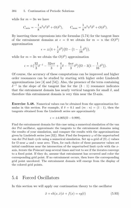
384 5. Continuation of Periodic Solutions
while for m = 3n we have
Cmin = −18n2π2δ2 + O(δ3), Cmax =
18n2π2δ2 + O(δ3).
By inserting these expressions into the formulas (5.74) for the tangent linesof the entrainment domains at ε = 0 we obtain for m = n the O(δ4)approximation
ε = ±(4 +
12δ2)(Ω −
(1 − 1
16δ2)),
while for m = 3n we obtain the O(δ3) approximation
ε = ±(32
3δ−1 − 32nπ
3+
43δ − 4nπ
3δ2)(Ω − 3
(1 − 1
16δ2)).
Of course, the accuracy of these computations can be improved and higherorder resonances can be studied by starting with higher order Lindstedtapproximations (see [4] and [54]). Also, the presence of the term containingδ−1 in the slope of the tangent line for the (3 : 1) resonance indicatesthat the entrainment domain has nearly vertical tangents for small δ, andtherefore this entrainment domain is very thin near the Ω-axis.
Exercise 5.48. Numerical values can be obtained from the approximation for-mulas in this section. For example, if δ = 0.1 and (m : n) = (1 : 1), then thetangents obtained from the Lindstedt series are approximately
ε = ±4.005(Ω − 0.999).
Find the entrainment domain for this case using a numerical simulation of the vander Pol oscillator, approximate the tangents to the entrainment domains usingthe results of your simulation, and compare the results with the approximationsgiven by Lindstedt series (see [32]). Hint: Find the frequency ω of the unperturbedvan der Pol limit cycle using a numerical simulation. Set up a grid of (Ω, ε) valuesfor Ω near ω and ε near zero. Then, for each choice of these parameter values setinitial conditions near the intersection of the unperturbed limit cycle with the x-axis, iterate the Poincare map several times and test to see if the iterates convergeto a fixed point. If they do, assume that entrainment has occurred and color thecorresponding grid point. If no entrainment occurs, then leave the correspondinggrid point uncolored. The entrainment domain will emerge from the display ofthe colored grid points.
5.4 Forced Oscillators
In this section we will apply our continuation theory to the oscillator
x + εh(x, x)x + f(x) = εg(t) (5.93)
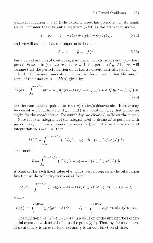
5.4 Forced Oscillators 385
where the function t → g(t), the external force, has period 2π/Ω. As usual,we will consider the differential equation (5.93) as the first order system
x = y, y = −f(x) + ε(g(t) − h(x, y)y), (5.94)
and we will assume that the unperturbed system
x = y, y = −f(x) (5.95)
has a period annulus A containing a resonant periodic solution Γm/n whoseperiod 2π/ω is in (m : n) resonance with the period of g. Also, we willassume that the period function on A has a nonzero derivative at Γm/n.
Under the assumptions stated above, we have proved that the simplezeros of the function φ → M(φ) given by
M(φ) =∫ n2π/ω
0y(t + φ, ξ)
(g(t) − h(x(t + φ, ξ), y(t + φ, ξ))y(t + φ), ξ)
)dt
(5.96)
are the continuation points for (m : n) (ultra)subharmonics. Here φ maybe viewed as a coordinate on Γm/n and ξ is a point on Γm/n that defines anorigin for the coordinate φ. For simplicity, we choose ξ to lie on the x-axis.
Note that the integrand of the integral used to define M is periodic withperiod n2π/ω. If we suppress the variable ξ and change the variable ofintegration to s = t + φ, then
M(φ) =∫ φ+n2π/ω
φ
(y(s)g(s − φ) − h(x(s), y(s))y2(s)
)ds.
The function
θ →∫ θ+n2π/ω
θ
(y(s)g(s − φ) − h(x(s), y(s))y2(s)
)ds
is constant for each fixed value of φ. Thus, we can represent the bifurcationfunction in the following convenient form:
M(φ) =∫ n2π/ω
0
(y(s)g(s − φ) − h(x(s), y(s))y2(s)
)ds = I1(φ) + I2,
where
I1(φ) :=∫ n2π/ω
0y(s)g(s − φ) ds, I2 :=
∫ n2π/ω
0h(x(s), y(s))y2(s) ds.
The function t → (x(−t),−y(−t)) is a solution of the unperturbed differ-ential equation with initial value at the point (ξ, 0). Thus, by the uniquenessof solutions, x is an even function and y is an odd function of time.
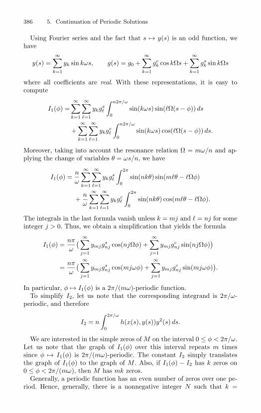
386 5. Continuation of Periodic Solutions
Using Fourier series and the fact that s → y(s) is an odd function, wehave
y(s) =∞∑
k=1
yk sin kωs, g(s) = g0 +∞∑
k=1
gck cos kΩs +
∞∑k=1
gsk sin kΩs
where all coefficients are real. With these representations, it is easy tocompute
I1(φ) =∞∑
k=1
∞∑=1
ykgs
∫ n2π/ω
0sin(kωs) sin(Ω(s − φ)) ds
+∞∑
k=1
∞∑=1
ykgc
∫ n2π/ω
0sin(kωs) cos(Ω(s − φ)) ds.
Moreover, taking into account the resonance relation Ω = mω/n and ap-plying the change of variables θ = ωs/n, we have
I1(φ) =n
ω
∞∑k=1
∞∑=1
ykgs
∫ 2π
0sin(nkθ) sin(mθ − Ωφ)
+n
ω
∞∑k=1
∞∑=1
ykgc
∫ 2π
0sin(nkθ) cos(mθ − Ωφ).
The integrals in the last formula vanish unless k = mj and = nj for someinteger j > 0. Thus, we obtain a simplification that yields the formula
I1(φ) =nπ
ω
( ∞∑j=1
ymjgsnj cos(njΩφ) +
∞∑j=1
ymjgcnj sin(njΩφ)
)=
nπ
ω
( ∞∑j=1
ymjgsnj cos(mjωφ) +
∞∑j=1
ymjgcnj sin(mjωφ)
).
In particular, φ → I1(φ) is a 2π/(mω)-periodic function.To simplify I2, let us note that the corresponding integrand is 2π/ω-
periodic, and therefore
I2 = n
∫ 2π/ω
0h(x(s), y(s))y2(s) ds.
We are interested in the simple zeros of M on the interval 0 ≤ φ < 2π/ω.Let us note that the graph of I1(φ) over this interval repeats m timessince φ → I1(φ) is 2π/(mω)-periodic. The constant I2 simply translatesthe graph of I1(φ) to the graph of M . Also, if I1(φ) − I2 has k zeros on0 ≤ φ < 2π/(mω), then M has mk zeros.
Generally, a periodic function has an even number of zeros over one pe-riod. Hence, generally, there is a nonnegative integer N such that k =
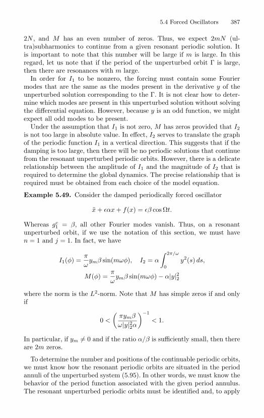
5.4 Forced Oscillators 387
2N , and M has an even number of zeros. Thus, we expect 2mN (ul-tra)subharmonics to continue from a given resonant periodic solution. Itis important to note that this number will be large if m is large. In thisregard, let us note that if the period of the unperturbed orbit Γ is large,then there are resonances with m large.
In order for I1 to be nonzero, the forcing must contain some Fouriermodes that are the same as the modes present in the derivative y of theunperturbed solution corresponding to the Γ. It is not clear how to deter-mine which modes are present in this unperturbed solution without solvingthe differential equation. However, because y is an odd function, we mightexpect all odd modes to be present.
Under the assumption that I1 is not zero, M has zeros provided that I2is not too large in absolute value. In effect, I2 serves to translate the graphof the periodic function I1 in a vertical direction. This suggests that if thedamping is too large, then there will be no periodic solutions that continuefrom the resonant unperturbed periodic orbits. However, there is a delicaterelationship between the amplitude of I1 and the magnitude of I2 that isrequired to determine the global dynamics. The precise relationship that isrequired must be obtained from each choice of the model equation.
Example 5.49. Consider the damped periodically forced oscillator
x + εαx + f(x) = εβ cos Ωt.
Whereas gc1 = β, all other Fourier modes vanish. Thus, on a resonant
unperturbed orbit, if we use the notation of this section, we must haven = 1 and j = 1. In fact, we have
I1(φ) =π
ωymβ sin(mωφ), I2 = α
∫ 2π/ω
0y2(s) ds,
M(φ) =π
ωymβ sin(mωφ) − α|y|22
where the norm is the L2-norm. Note that M has simple zeros if and onlyif
0 <
(πymβ
ω|y|22α
)−1
< 1.
In particular, if ym = 0 and if the ratio α/β is sufficiently small, then thereare 2m zeros.
To determine the number and positions of the continuable periodic orbits,we must know how the resonant periodic orbits are situated in the periodannuli of the unperturbed system (5.95). In other words, we must know thebehavior of the period function associated with the given period annulus.The resonant unperturbed periodic orbits must be identified and, to apply
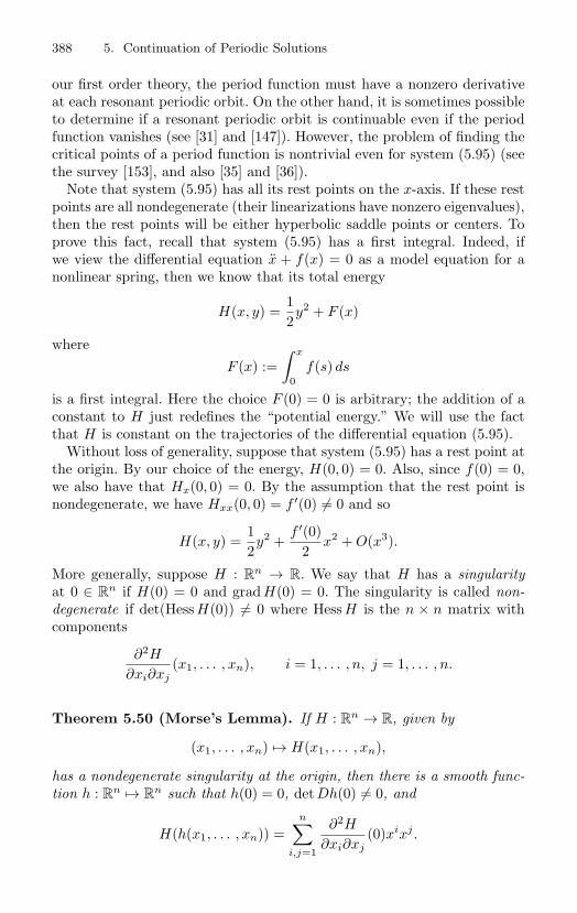
388 5. Continuation of Periodic Solutions
our first order theory, the period function must have a nonzero derivativeat each resonant periodic orbit. On the other hand, it is sometimes possibleto determine if a resonant periodic orbit is continuable even if the periodfunction vanishes (see [31] and [147]). However, the problem of finding thecritical points of a period function is nontrivial even for system (5.95) (seethe survey [153], and also [35] and [36]).
Note that system (5.95) has all its rest points on the x-axis. If these restpoints are all nondegenerate (their linearizations have nonzero eigenvalues),then the rest points will be either hyperbolic saddle points or centers. Toprove this fact, recall that system (5.95) has a first integral. Indeed, ifwe view the differential equation x + f(x) = 0 as a model equation for anonlinear spring, then we know that its total energy
H(x, y) =12y2 + F (x)
whereF (x) :=
∫ x
0f(s) ds
is a first integral. Here the choice F (0) = 0 is arbitrary; the addition of aconstant to H just redefines the “potential energy.” We will use the factthat H is constant on the trajectories of the differential equation (5.95).
Without loss of generality, suppose that system (5.95) has a rest point atthe origin. By our choice of the energy, H(0, 0) = 0. Also, since f(0) = 0,we also have that Hx(0, 0) = 0. By the assumption that the rest point isnondegenerate, we have Hxx(0, 0) = f ′(0) = 0 and so
H(x, y) =12y2 +
f ′(0)2
x2 + O(x3).
More generally, suppose H : Rn → R. We say that H has a singularity
at 0 ∈ Rn if H(0) = 0 and gradH(0) = 0. The singularity is called non-
degenerate if det(Hess H(0)) = 0 where Hess H is the n × n matrix withcomponents
∂2H
∂xi∂xj(x1, . . . , xn), i = 1, . . . , n, j = 1, . . . , n.
Theorem 5.50 (Morse’s Lemma). If H : Rn → R, given by
(x1, . . . , xn) → H(x1, . . . , xn),
has a nondegenerate singularity at the origin, then there is a smooth func-tion h : R
n → Rn such that h(0) = 0, det Dh(0) = 0, and
H(h(x1, . . . , xn)) =n∑
i,j=1
∂2H
∂xi∂xj(0)xixj .
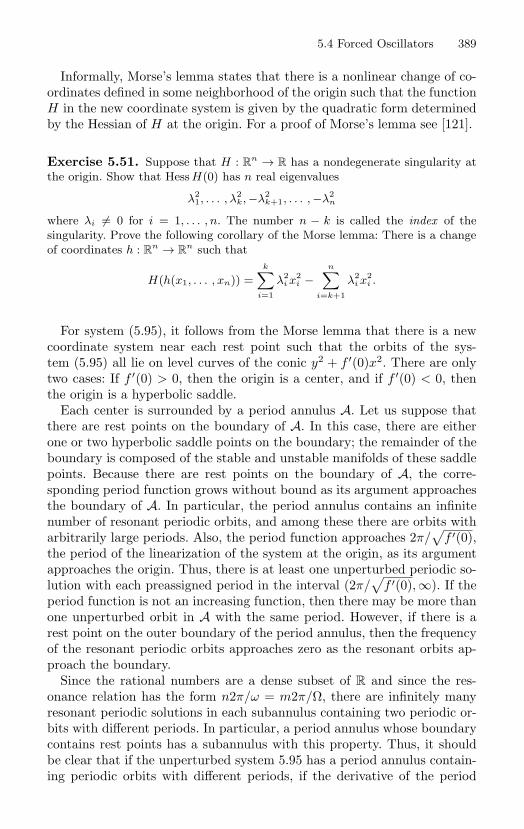
5.4 Forced Oscillators 389
Informally, Morse’s lemma states that there is a nonlinear change of co-ordinates defined in some neighborhood of the origin such that the functionH in the new coordinate system is given by the quadratic form determinedby the Hessian of H at the origin. For a proof of Morse’s lemma see [121].
Exercise 5.51. Suppose that H : Rn → R has a nondegenerate singularity at
the origin. Show that Hess H(0) has n real eigenvalues
λ21, . . . , λ2
k, −λ2k+1, . . . , −λ2
n
where λi = 0 for i = 1, . . . , n. The number n − k is called the index of thesingularity. Prove the following corollary of the Morse lemma: There is a changeof coordinates h : R
n → Rn such that
H(h(x1, . . . , xn)) =k∑
i=1
λ2i x
2i −
n∑i=k+1
λ2i x
2i .
For system (5.95), it follows from the Morse lemma that there is a newcoordinate system near each rest point such that the orbits of the sys-tem (5.95) all lie on level curves of the conic y2 + f ′(0)x2. There are onlytwo cases: If f ′(0) > 0, then the origin is a center, and if f ′(0) < 0, thenthe origin is a hyperbolic saddle.
Each center is surrounded by a period annulus A. Let us suppose thatthere are rest points on the boundary of A. In this case, there are eitherone or two hyperbolic saddle points on the boundary; the remainder of theboundary is composed of the stable and unstable manifolds of these saddlepoints. Because there are rest points on the boundary of A, the corre-sponding period function grows without bound as its argument approachesthe boundary of A. In particular, the period annulus contains an infinitenumber of resonant periodic orbits, and among these there are orbits witharbitrarily large periods. Also, the period function approaches 2π/
√f ′(0),
the period of the linearization of the system at the origin, as its argumentapproaches the origin. Thus, there is at least one unperturbed periodic so-lution with each preassigned period in the interval (2π/
√f ′(0),∞). If the
period function is not an increasing function, then there may be more thanone unperturbed orbit in A with the same period. However, if there is arest point on the outer boundary of the period annulus, then the frequencyof the resonant periodic orbits approaches zero as the resonant orbits ap-proach the boundary.
Since the rational numbers are a dense subset of R and since the res-onance relation has the form n2π/ω = m2π/Ω, there are infinitely manyresonant periodic solutions in each subannulus containing two periodic or-bits with different periods. In particular, a period annulus whose boundarycontains rest points has a subannulus with this property. Thus, it shouldbe clear that if the unperturbed system 5.95 has a period annulus contain-ing periodic orbits with different periods, if the derivative of the period
390 5. Continuation of Periodic Solutions
function does not vanish on each resonant orbit in the annulus, and if thedamping is sufficiently small, then there will be a large number of perturbed(ultra)subharmonics.
Are there infinitely many (ultra)subharmonics? Our analysis does notanswer this question. To see why, recall our main result: If the function Min display (5.96) has simple zeros along an (m : n) resonant unperturbedperiodic orbit, then for sufficiently small ε there are 2mN perturbed (ul-tra)subharmonics where N is some positive integer. However, if we consideran infinite number of resonant orbits, for example a sequence of periodicorbits that approach the boundary of our period annulus, then it mighthappen that the infinite number of requirements for ε to be sufficientlysmall cannot be satisfied simultaneously without taking ε = 0. For thisreason, we cannot conclude that there is an ε > 0 such that the corre-sponding perturbed system has infinitely many periodic solutions even if(ultra)subharmonics continue from all resonant unperturbed periodic or-bits. Thus, we are left with evidence that oscillators with an infinite numberof (ultra)subharmonics exist, but we have no proof. However, let us notethat if an oscillator has an infinite number of hyperbolic periodic orbitsof saddle type all contained in some compact subset of its extended phasespace, then we might expect the dynamical behavior of the oscillator ina neighborhood of this set to be very complex: orbits in the neighbor-hood might tend to follow a stable manifold, pass by a saddle point, followthe motion on its unstable manifold, pass near another stable manifold,and then repeat the process. Whatever the exact nature of such a flow, itshould be clear that we cannot hope to understand the dynamics of os-cillators without considering this possible behavior. It turns out that byusing some new ideas introduced in Chapter 6 we will be able to show thatsome periodically perturbed oscillators do indeed have an infinite numberof (ultra)subharmonics and that their flows are “chaotic”.
6Homoclinic Orbits,Melnikov’s Method, and Chaos
In the last chapter, we discussed the near resonance continuation theoryfor periodic orbits of periodically perturbed oscillators. In case the un-perturbed oscillator has a regular period annulus, we found that there isgenerally an infinite number of resonances at which a first order pertur-bation theory can be used to prove the existence of perturbed periodicorbits. However, we cannot conclude from the results of our analysis thatthe perturbed oscillator has infinitely many periodic orbits. To do so wouldseem to require a condition that might be impossible to satisfy. Indeed, thenonzero amplitude of the perturbation would have to be made sufficientlysmall an infinite number of times corresponding to the unperturbed, reso-nant, periodic orbits in an infinite sequence that approaches the boundaryof the period annulus. The subject of this chapter is a perturbation theorythat is valid at the boundary of the period annulus. When the theory is ap-plied, the amplitude of the perturbation is only required to be sufficientlysmall once.
Generally, the boundary of a period annulus for an unperturbed oscil-lator consists of one or more saddle points connected by homoclinic orheteroclinic orbits. Let us define a saddle connection to be an orbit whoseα- and ω-limit sets are hyperbolic saddle points. A saddle connection iscalled a homoclinic orbit if its α- and ω-limit sets coincide. On the otherhand, the saddle connection is called a heteroclinic orbit if its α-limit setis disjoint from its ω-limit set.
If the saddle points on the boundary of our period annulus are hyper-bolic, then they persist along with their stable and unstable manifolds.For simplicity, let us consider the case where there is just one hyperbolic
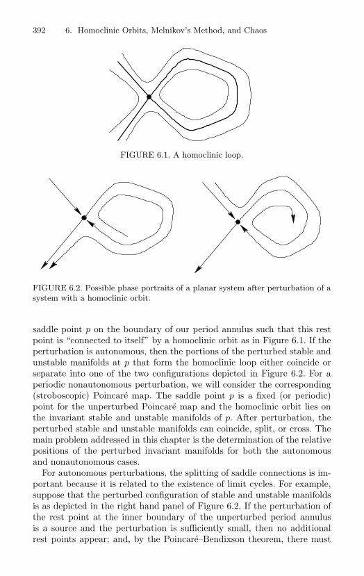
392 6. Homoclinic Orbits, Melnikov’s Method, and Chaos
FIGURE 6.1. A homoclinic loop.
FIGURE 6.2. Possible phase portraits of a planar system after perturbation of asystem with a homoclinic orbit.
saddle point p on the boundary of our period annulus such that this restpoint is “connected to itself” by a homoclinic orbit as in Figure 6.1. If theperturbation is autonomous, then the portions of the perturbed stable andunstable manifolds at p that form the homoclinic loop either coincide orseparate into one of the two configurations depicted in Figure 6.2. For aperiodic nonautonomous perturbation, we will consider the corresponding(stroboscopic) Poincare map. The saddle point p is a fixed (or periodic)point for the unperturbed Poincare map and the homoclinic orbit lies onthe invariant stable and unstable manifolds of p. After perturbation, theperturbed stable and unstable manifolds can coincide, split, or cross. Themain problem addressed in this chapter is the determination of the relativepositions of the perturbed invariant manifolds for both the autonomousand nonautonomous cases.
For autonomous perturbations, the splitting of saddle connections is im-portant because it is related to the existence of limit cycles. For example,suppose that the perturbed configuration of stable and unstable manifoldsis as depicted in the right hand panel of Figure 6.2. If the perturbation ofthe rest point at the inner boundary of the unperturbed period annulusis a source and the perturbation is sufficiently small, then no additionalrest points appear; and, by the Poincare–Bendixson theorem, there must
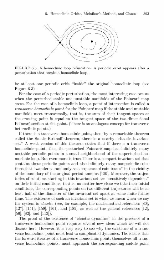
6. Homoclinic Orbits, Melnikov’s Method, and Chaos 393
FIGURE 6.3. A homoclinic loop bifurcation: A periodic orbit appears after aperturbation that breaks a homoclinic loop.
be at least one periodic orbit “inside” the original homoclinic loop (seeFigure 6.3).
For the case of a periodic perturbation, the most interesting case occurswhen the perturbed stable and unstable manifolds of the Poincare mapcross. For the case of a homoclinic loop, a point of intersection is called atransverse homoclinic point for the Poincare map if the stable and unstablemanifolds meet transversally, that is, the sum of their tangent spaces atthe crossing point is equal to the tangent space of the two-dimensionalPoincare section at this point. (There is an analogous concept for transverseheteroclinic points.)
If there is a transverse homoclinic point, then, by a remarkable theoremcalled the Smale–Birkhoff theorem, there is a nearby “chaotic invariantset.” A weak version of this theorem states that if there is a transversehomoclinic point, then the perturbed Poincare map has infinitely manyunstable periodic points in a small neighborhood of the unperturbed ho-moclinic loop. But even more is true: There is a compact invariant set thatcontains these periodic points and also infinitely many nonperiodic solu-tions that “wander as randomly as a sequence of coin tosses” in the vicinityof the boundary of the original period annulus [159]. Moreover, the trajec-tories of solutions starting in this invariant set are “sensitively dependent”on their initial conditions; that is, no matter how close we take their initialconditions, the corresponding points on two different trajectories will be atleast half of the diameter of the invariant set apart at some finite futuretime. The existence of such an invariant set is what we mean when we saythe system is chaotic (see, for example, the mathematical references [80],[127], [151], [159], [161], and [185], as well as the general references [12],[56], [82], and [113]).
The proof of the existence of “chaotic dynamics” in the presence of atransverse homoclinic point requires several new ideas which we will notdiscuss here. However, it is very easy to see why the existence of a trans-verse homoclinic point must lead to complicated dynamics. The idea is thatthe forward iterates of a transverse homoclinic point, themselves all trans-verse homoclinic points, must approach the corresponding saddle point
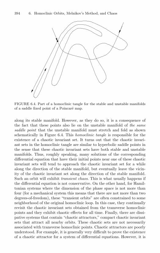
394 6. Homoclinic Orbits, Melnikov’s Method, and Chaos
FIGURE 6.4. Part of a homoclinic tangle for the stable and unstable manifoldsof a saddle fixed point of a Poincare map.
along its stable manifold. However, as they do so, it is a consequence ofthe fact that these points also lie on the unstable manifold of the samesaddle point that the unstable manifold must stretch and fold as shownschematically in Figure 6.4. This homoclinic tangle is responsible for theexistence of a chaotic invariant set. It turns out that the chaotic invari-ant sets in the homoclinic tangle are similar to hyperbolic saddle points inthe sense that these chaotic invariant sets have both stable and unstablemanifolds. Thus, roughly speaking, many solutions of the correspondingdifferential equation that have their initial points near one of these chaoticinvariant sets will tend to approach the chaotic invariant set for a whilealong the direction of the stable manifold, but eventually leave the vicin-ity of the chaotic invariant set along the direction of the stable manifold.Such an orbit will exhibit transient chaos. This is what usually happens ifthe differential equation is not conservative. On the other hand, for Hamil-tonian systems where the dimension of the phase space is not more thanfour (for a mechanical system this means that there are not more than twodegrees-of-freedom), these “transient orbits” are often constrained to someneighborhood of the original homoclinic loop. In this case, they continuallyrevisit the chaotic invariant sets obtained from the transverse homoclinicpoints and they exhibit chaotic effects for all time. Finally, there are dissi-pative systems that contain “chaotic attractors,” compact chaotic invariantsets that attract all nearby orbits. These chaotic sets are not necessarilyassociated with transverse homoclinic points. Chaotic attractors are poorlyunderstood. For example, it is generally very difficult to prove the existenceof a chaotic attractor for a system of differential equations. However, it is

6. Homoclinic Orbits, Melnikov’s Method, and Chaos 395
not at all difficult to “see” a chaotic attractor using numerical simulations(see Exercise 6.1).
We will show how to detect the splitting of saddle connections by defin-ing a function that determines the separation of the perturbed invariantmanifolds as a function of the bifurcation parameters. It turns out that theappropriate function is the limit of the subharmonic Melnikov function asthe base points on the periodic orbits approach the boundary. For exam-ple, for the case of the forced oscillator (5.94) where we have defined thesubharmonic Melnikov function M in display (5.96), the function we seekis the limit of M as ξ approaches a point on the boundary that is not a restpoint. The limit function, again denoted by M , is again called the Melnikovfunction. In fact, the Melnikov function for the differential equation (5.94)is given by
M(φ) =∫ ∞
−∞y(t + φ, ξ)
(g(t) − h(x(t + φ, ξ), y(t + φ, ξ))y(t + φ, ξ)
)dt
or, after the obvious change of variables, by
M(φ) =∫ ∞
−∞y(s, ξ)
(g(s − φ) − h(x(s, ξ), y(s, ξ))y(s, ξ)
)ds
where ξ is a base point on the boundary and the coordinate φ specifiesposition on the boundary.
For an autonomous perturbation, the Melnikov function does not dependon the initial point for the unperturbed solution on the boundary. In thiscase the sign of the Melnikov function determines the direction in which theinvariant manifolds split. For a time periodic perturbation, the Melnikovfunction does depend on the initial point on the boundary, and its sim-ple zeros correspond to positions where the perturbed stable and unstablemanifolds intersect transversally for sufficiently small ε = 0.
The derivation and analysis of the Melnikov function for autonomousperturbations is of course a special case of its derivation for nonautonomousperturbations. However, since the analysis for autonomous perturbationsis conceptually simpler, we will give a detailed discussion of this case first.
Exercise 6.1. Write a report on numerical simulations of the Lorenz system
x = σ(y − x), y = ρx − y − xz, z = −βz + xy
(see the original paper of Edward N. Lorenz [111] or any book on dynamicalsystems theory). Start by setting the parameter values β = 8
3 , ρ = 28, andσ = 10. Choose an initial condition in the first quadrant, for instance near theunstable manifold of the saddle point at the origin, integrate forward in time,and display the resulting approximate orbit using three-dimensional graphics.The “Lorenz butterfly attractor” will appear. Also graph one of the observables,say t → y(t), and compare the time series you obtain with the graph of a periodic
396 6. Homoclinic Orbits, Melnikov’s Method, and Chaos
function. Choose a second initial condition near the initial condition you startedwith and plot the simulated graphs of t → y(t) for both initial conditions. Notethat these graphs will stay close together for a while (as they must due to thesmoothness of solutions with respect to initial conditions), but eventually theywill diverge. For this reason, it is impossible to predict the position of the statevector from the initial conditions over long time periods with an accuracy thatis small compared with the diameter of the attractor; the system is extremelysensitive to changes in the initial conditions. This is one of the hallmarks of achaotic flows.
6.1 Autonomous Perturbations:Separatrix Splitting
Consider the planar system
u = f(u, λ), u ∈ R2, λ ∈ R
n (6.1)
and let ξ0 ∈ R2 be a regular point for the unperturbed system
u = f(u, 0). (6.2)
As usual, let t → u(t, ξ, λ) denote the solution of the differential equa-tion (6.1) such that u(0, ξ, λ) = ξ, define f⊥(u) = Rf(u, 0) where
R :=(
0 −11 0
),
and let t → Ψ(t, ξ) denote the flow of the orthogonal system u = f⊥(u).Here, of course, t → Ψ(t, ξ0) is transverse to t → u(t, ξ0, 0) at ξ0.
Define
Σ := Ψ(t, ξ0) : t ∈ R, (6.3)
and suppose that we have devised some construction that produces twofamilies of solutions of the differential equation (6.1), each parametrized byλ, whose members are all transverse to Σ such that at λ = 0 the corre-sponding solutions coincide with the unperturbed solution t → u(t, ξ0, 0).Our objective is to obtain some information about the rate of separationof the solutions belonging to the two parametrized families of solutions. Infact, we will obtain a general conclusion about this separation rate follow-ing the presentation given by Stephen Schecter [158]. This result will thenbe used to address the problem of breaking saddle connections.
Suppose that our construction produces two smooth functions ρi : Rn →
R, i = 1, 2, given by λ → ρi(λ) such that ρi(0) = 0 where ρi(λ) gives thepoint of intersection of the ith family with Σ. We desire information about
6.1 Autonomous Perturbations: Separatrix Splitting 397
the separation of the two solution families of the differential equation (6.1)given by
γi(t, λ) := u(t, Ψ(ρi(λ), ξ0), λ), i = 1, 2. (6.4)
Let us view these families as “variations” of the unperturbed solution; thatis, γi is a family of solutions containing the unperturbed solution at λ = 0
γi(t, 0) = u(t, ξ0, 0), i = 1, 2.
Also, γi has initial value on the transverse section Σ. In fact,
γi(0, λ) = Ψ(ρi(λ), ξ0).
The separation of the variations from the unperturbed solution is definedby the function λ → ρ1(λ) − ρ2(λ); it measures the distance between thepoints where our variations cross Σ. Of course, in a perturbation problem,it is unlikely that we will be given the functions ρ1 and ρ2 explicitly. Atbest, we will be able to infer their existence (probably by an application ofthe implicit function theorem). However, for small λ, a good approximationof the separation is given by the separation function sep : R
n → R definedby
sep(λ) := 〈Ψ(ρ1(λ), ξ0) − Ψ(ρ2(λ), ξ0), f⊥(ξ0)〉= f(ξ0, 0) ∧ (Ψ(ρ1(λ), ξ0) − Ψ(ρ2(λ), ξ0)).
Let us note that, sep(0) = 0. Also, sep(λ) = 0 if and only if the solutionsγ1(t, λ) and γ2(t, λ) are identical. This last fact follows because a solutionof an initial value problem is unique.
As usual, we can determine the local nature of S := λ : sep(λ) = 0provided that there is at least one j = 1, . . . , n such that sepλj
(0) = 0. Infact, if this condition holds, then by the implicit function theorem S is asurface of dimension n − 1 passing through 0 ∈ R
n whose normal vector atthis point is just grad(sep)(0).
What have we done so far? In analogy with our continuation theory forperiodic solutions, we have defined a function akin to the displacementfunction and we have reduced the study of its zero set to an applicationof the implicit function theorem. Let us make this reduction useful byidentifying the partial derivatives of the separation function.
To identify the partial derivatives of the separation function using theoriginal differential equation (6.1), we expect to solve a variational equa-tion. But to obtain a nontrivial variational equation we must have sometime dependence in the separation function. This requirement motivatesthe definition of the time-dependent separation function S : R × R
n → R
given by
S(t, λ) := 〈γ1(t, λ) − γ2(t, λ), f⊥(ϕt(ξ0))〉= f(ϕt(ξ0), 0) ∧ (γ1(t, λ) − γ2(t, λ))
398 6. Homoclinic Orbits, Melnikov’s Method, and Chaos
where ϕt is the flow of the system (6.2). Since S(0, λ) = sep(λ), the mainidea—originally due to Melnikov—is to compute the desired partial deriva-tives of the separation function sep from the corresponding partial deriva-tives of the time-dependent separation function S.
Let us define two auxiliary functions
Si(t, λ) := 〈γi(t, λ), f⊥(ϕt(ξ0))〉= f(ϕt(ξ0), 0) ∧ γi(t, λ)
for i = 1, 2, and note that S(t, λ) = S1(t, λ) − S2(t, λ). To compute therequired partial derivatives, start with the formula
Siλj
(t, 0) = f(ϕt(ξ0), 0) ∧ γiλj
(t, 0), (6.5)
and use the fact that the function t → γi(t, λ) is a solution of the differentialequation (6.1) to obtain the variational equation
γiλi
(t, 0) = fu(ϕt(ξ0), 0)γiλj
(t, 0) + fλj(ϕt(ξ0), 0). (6.6)
Next, define A(t) := fu(ϕt(ξ0), 0) and use equation (6.5) to obtain thedifferential equation
Siλj
(t, 0) = fu(ϕt(ξ0), 0)f(ϕt(ξ0), 0) ∧ γiλj
(t, 0) + f(ϕt(ξ0), 0) ∧ γiλj
(t, 0)
= A(t)f(ϕt(ξ0), 0) ∧ γiλj
(t, 0) + f(ϕt(ξ0), 0) ∧ A(t)γiλj
(t, 0)+ f(ϕt(ξ0), 0) ∧ fλj
(ϕt(ξ0), 0). (6.7)
Formula (6.7) can be simplified by an application of the following easilyproved proposition from vector analysis: If A is a 2×2 matrix and v, w ∈ R
2,then
Av ∧ w + v ∧ Aw = (trA)v ∧ w.
In fact, with the aid of this proposition, we have
Siλj
(t, 0) = div f(ϕt(ξ0), 0)f(ϕt(ξ0), 0) ∧ γiλj
(t, 0)+ f(ϕt(ξ0), 0) ∧ fλj
(ϕt(ξ0), 0)
= div f(ϕt(ξ0), 0)Siλj
(t, 0) + f(ϕt(ξ0), 0) ∧ fλj (ϕt(ξ0), 0). (6.8)
The differential equation (6.8) is a linear variational equation for thefunction t → Si
λj(t, 0). To solve it, let us assume that we know the behavior
of γ1(t, 0) as t → −∞ and the behavior of γ2(t, 0) as t → ∞. If we define
K(t) := e− ∫ t0 div f(ϕt(ξ0),0) ds
and integrate both sides of the differential equation
d
dt
(K(t)Si
λj(t, 0)
)= K(t)f(ϕt(ξ0)) ∧ fλj
(ϕt(ξ0), 0),
6.1 Autonomous Perturbations: Separatrix Splitting 399
then we obtain the identities
S1λj
(0, 0) = K(t)S1λj
(t, 0) +∫ 0
t
K(s)f(ϕs(ξ0)) ∧ fλj (ϕs(ξ0), 0) ds,
−S2λj
(0, 0) = −K(t)S2λj
(t, 0) +∫ t
0K(s)f(ϕs(ξ0)) ∧ fλj (ϕs(ξ0), 0) ds.
Note that the right hand side of each of these identities is constant withrespect to t. Using this fact, the desired partial derivative is given by
sepλj(0) = lim
t→−∞
[K(t)f(ϕt(ξ0)) ∧ γ1
λj(t, 0)
+∫ 0
t
K(s)f(ϕs(ξ0)) ∧ fλj(ϕs(ξ0), 0) ds
]+ lim
t→∞
[− K(t)f(ϕt(ξ0)) ∧ γ2
λj(t, 0)
+∫ t
0K(s)f(ϕs(ξ0)) ∧ fλj (ϕs(ξ0), 0) ds
]. (6.9)
We reiterate that the indicated limits exist because the quantities in squarebrackets are constants. Of course, the summands of each expression insquare brackets are not necessarily constants.
The representation (6.9) of the partial derivatives of the separation func-tion is useful because it is general. However, let us return to the maintopic of this section and apply this result to the perturbation of saddleconnections.
Suppose that ξ0 denotes a point on a saddle connection for system (6.2)connecting the hyperbolic saddle points p0 and q0 (maybe p0 = q0); thatis,
limt→−∞ ϕt(ξ0) = p0, lim
t→∞ ϕt(ξ0) = q0.
Also, let Σ denote the section at ξ0 defined in display (6.3). By the im-plicit function theorem, if λ is sufficiently small, then there are perturbedhyperbolic saddle points
pλ = p0 + O(λ), qλ = q0 + O(λ)
for the system (6.1). Define t → γ1(t, λ) to be the solution of the sys-tem (6.1) with initial condition on Σ (as in equation (6.4)) that lies onthe unstable manifold of pλ, and let t → γ2(t, λ) denote the correspondingsolution on the stable manifold of the hyperbolic saddle point qλ. The factthat the stable and unstable manifolds γi, i = 1, 2, intersect the fixed curveΣ is a consequence of Theorem 4.1. To see this, add the equation λ = 0to the system (6.1) and use the smoothness of the center stable manifoldcorresponding to each rest point of the augmented system correspondingto the saddle points p0 and q0.
We will outline a proof of the following proposition:
400 6. Homoclinic Orbits, Melnikov’s Method, and Chaos
Proposition 6.2. If system (6.1) with λ = 0 has a saddle connection andif γ1 and γ2, as in display (6.4), are defined to be solutions on the unstableand stable manifolds of the perturbed saddle points, then
limt→−∞ K(t)f(ϕt(ξ0)) ∧ γ1
λj(t, 0) = 0, (6.10)
limt→∞ K(t)f(ϕt(ξ0)) ∧ γ2
λj(t, 0) = 0. (6.11)
Moreover,
sepλj(0) =
∫ ∞
−∞e− ∫ t
0 div f(ϕs(ξ0),0) dsf(ϕt(ξ0), 0) ∧ fλj (ϕt(ξ0), 0) dt. (6.12)
The important formula (6.12) for the partial derivatives of the separationfunction with respect to the parameters was probably known to Poincare.It was also discovered independently by several different authors (see, forexample, [120], [149], and [163]). However, the integral is now most oftencalled the Melnikov integral.
Since sep(0) = 0, the Taylor series of the separation function at λ = 0 is
sep(λ) =n∑
j=1
λj sepλj(0) + O(|λ|2). (6.13)
In particular, if n = 1 and ε := λ1, then
sep(ε) = ε(sepε(0) + O(ε)). (6.14)
Therefore, if sepε(0) = 0 and if |ε| is sufficiently small, then formula (6.12)can be used to determine the sign of sep(ε), and therefore the splittingdirection of the perturbed stable and unstable manifolds relative to thedirection determined by f⊥(ξ0).
An outline for a proof of the limit (6.11) will be given; a proof for thelimit (6.10) can be constructed similarly.
View the vector field f as a mapping f : R2 × R
n → R2. Since f(q0, 0) =
0 and since fu(q0, 0) : R2 → R
2 is a nonsingular linear transformation(it has no eigenvalue on the imaginary axis in the complex plane by thehyperbolicity of q0), the implicit function theorem implies there is a mapq : R
n → R2 defined near λ = 0 such that q(0) = q0 and f(q(λ), λ) ≡ 0. By
the continuous dependence of the eigenvalues of a matrix on its coefficients,we have that q(λ) is a hyperbolic saddle point for |λ| sufficiently small.
As mentioned above, the stable manifold of q(λ) varies smoothly withλ by Theorem 4.1. In particular, the function (t, λ) → γ2(t, λ) dependssmoothly on t and λ, and limt→∞ γ2(t, λ) = q(λ). The matrix fu(q0, 0)has two real eigenvalues −µ1 < 0 < µ2. Moreover, as t → ∞ the curvet → γ2(t, 0) approaches the saddle point q0 tangent to the eigenspace cor-responding to the eigenvalue −µ.
6.1 Autonomous Perturbations: Separatrix Splitting 401
By an affine change of coordinates, if necessary, we may as well assumethat q0 is located at the origin and the unperturbed differential equationu = f(u, 0) has the form
x = −µx + f1(x, y), y = νy + f2(x, y) (6.15)
where both µ and ν are positive constants, and the functions f1 and f2together with their first order partial derivatives vanish at the origin. Inthese coordinates, the stable manifold of the hyperbolic saddle point at theorigin is given by the graph of a smooth function h : U → R where U ⊂ R
is an open interval containing the origin on the x-axis. Moreover, becausethe stable manifold is tangent to the x-axis at the origin, we have h(0) = 0and h′(0) = 0.
The estimate that we will use to compute the limit (6.11) is the contentof the following proposition.
Proposition 6.3. If |x0| is sufficiently small, then there is a positive con-stant c such that the solution of the system (6.15) starting at (x0, h(x0))satisfies the estimate
|x(t)| + |y(t)| ≤ ce−µt, t ≥ 0.
The next lemma (compare Theorem 2.42) will be used to prove Propo-sition 6.3.
Lemma 6.4. If t → x(t) is the solution of the initial value problem
x = −µx + g(x), x(0) = x0 ∈ R, µ > 0
where g is a smooth function such that g(0) = 0 and g′(0) = 0, then thereare constants ε > 0 and c > 0 such that |x(t)| ≤ ce−µt for t ≥ 0 whenever|x0| < ε.
Proof. The function defined by
G(x) :=
x−2g(x), x = 00, x = 0
is continuous at x = 0. Thus, there is some constant C such that |G(x)| ≤ Cfor sufficiently small |x|.
For x = 0, we have
− x
x2 − µ
x= −G(x).
If y := 1/x, then y − µy = −G(x(t)) and
e−µty(t) = y(0) −∫ t
0e−µsG(x(s)) ds.
402 6. Homoclinic Orbits, Melnikov’s Method, and Chaos
Thus, we have the estimate
|e−µty(t)| ≥ |y(0)| −∫ t
0e−µs|G(x(s)| ds,
and for sufficiently small |x0|
|y(0)| ≤ |e−µty(t)| + C
∫ t
0e−µs ds. (6.16)
We are using the fact that if |x0| is sufficiently small, then |x(t)| < |x0|for t ≥ 0. This follows from the assumption that the point x = 0 is anattracting rest point for our one-dimensional differential equation. How-ever, a weaker assumption would also be sufficient. For example, it sufficesto assume that for |x0| sufficiently small, the interval (−|x0|, |x0|) is pos-itively invariant. This follows immediately by considering the direction ofthe vector field corresponding to our differential equation at the end pointsof the appropriately chosen interval.
After an elementary integration, inequality (6.16) states that
|y(0)| ≤ |e−µty(t)| +C
µ(1 − e−µt).
Moreover, because t ≥ 0, it follows that
|y(0)| ≤ |e−µty(t)| +C
µ,
and therefore1
|x0|− C
µ≤ 1
eµt|x(t)| .
If |x0| > 0 is sufficiently small, then
1|x0|
− C
µ>
1c
> 0
for some c > 0. Thus, we have that
|x(t)| ≤ ce−µt.
Remark: Schecter [158] proves a sharper lemma. Under the same hy-potheses as in Lemma 6.4, he proves that
limt→∞ eµtx(t) = L = 0.
Let us prove Proposition 6.3.
6.1 Autonomous Perturbations: Separatrix Splitting 403
Proof. Consider the change of coordinates for the system (6.15) given by
p = x, q = y − h(x).
In these coordinates, the saddle point stays fixed at the origin, but the sta-ble manifold is transformed to the p-axis. The restriction of the transformeddifferential equation to the p-axis is given by
p = −µp + f1(p, h(p)). (6.17)
If g(p) := f1(p, h(p)), then all the hypotheses of the lemma are satisfied,and we conclude that there is some |p0| = 0 such that solutions of thedifferential equation (6.17) satisfy |p(t)| ≤ ce−µt for some c > 0 and allt ≥ 0 whenever |p(0)| < |p0|. In the original coordinates, the correspondingsolution on the stable manifold is given by x(t) = p(t), y(t) = h(x(t)).Since y = h(x) is tangent to the x-axis at x = 0, there is a constant c1 > 0such that |h(x)| < c1x
2 for |x| sufficiently small. Thus, if the initial valueof the solution of the differential equation (6.15) on the stable manifold issufficiently close to the origin, then
|x(t)| + |y(t)| = |x(t)| + |h(x(t))| ≤ |x(t)|(1 + c1, |x(t)|) ≤ 2ce−µt.
To conclude our discussion of the limit (6.11), we must analyze theasymptotic behavior of the functions K(t), f(ϕt(ξ0), 0), and γ2
λj(t, 0). Let
us note first that since f(u, 0) is Lipschitz, we have
||f(u, 0)|| = ||f(u, 0) − f(0, 0)|| ≤ L||u||
for some constant L > 0. By the proposition,
||f(ϕt(ξ0), 0)|| ≤ Lce−µt.
Likewise, using the smoothness of u → f(u, 0), we have
div f(u, 0) = tr fu(0, 0) + R(u)
where, for sufficiently small ||u||, there is a constant c2 > 0 such that theremainder R satisfies ||R(u)|| ≤ c2||u||. Thus
K(t) = e− ∫ t0 ν−µ due− ∫ t
0 R(u(s)) ds
≤ e(µ−ν)tec2∫ t0 ce−µs ds
≤ c3e(µ−ν)t
for some c3 > 0. It follows that
limt→∞ K(t)f(ϕt(ξ0), 0) = 0.
404 6. Homoclinic Orbits, Melnikov’s Method, and Chaos
To complete the argument let us see that |γ2λj
(t, 0)| is bounded. For this,we use the smoothness of the stable manifold with respect to the parameterλ. There is no loss of generality if we assume that the hyperbolic saddleq(λ) remains at the origin with its stable manifold tangent to the x-axis asin system (6.15). Indeed, this geometry can be achieved by a parameter-dependent affine change of coordinates. More precisely, there is a smoothfunction (x, λ) → h(x, λ) defined near (x, y) = (0, 0) such that the stablemanifold is the graph of the function x → h(x, λ). Of course, we also havethat h(0, λ) ≡ 0 and hx(0, λ) ≡ 0. Using this representation of the stablemanifold,
γ2(t, λ) = (x(t, λ), h(x(t, λ), λ))
where t → x(t, λ) is a solution of a differential equation
x = −µx + g(x, λ)
similar to differential equation (6.17). After differentiation, we find that
γ2λj
(t, 0) = (xλj(t, 0), hx(x(t, 0), 0)xλj
(t, 0) + hλj(x(t, 0), 0)).
By the smoothness of the function h, both hx(x, 0) and hλj(x, 0) are
bounded for x in some fixed but sufficiently small interval containing x = 0.Thus, the boundedness of the function t → γ2
λj(t, 0) will be proved once we
show that t → xλj(t, 0) is bounded as t → ∞. To obtain this bound, let us
use the fact that t → xλj (t, 0) is a solution of the variational equation
w = −µw + gx(x(t, 0), 0)w + gλj (x(t, 0), 0). (6.18)
Because gx(0, 0) = 0 and the function g is smooth, we have the estimate
|gx(x, 0)| ≤ c1|x|
for some c1 > 0. In addition, since g(0, λ) ≡ 0, it follows that gλj (0, 0) = 0.Also, by the smoothness of g, the partial derivative gλj is locally Lipschitz.In fact, there is some c2 > 0 such that
|gλj(x, 0)| = |gλj
(x, 0) − gλj(0, 0)| ≤ c2|x|.
With the obvious choice of notation, the differential equation (6.18) hasthe form
w = (−µ + α(t))w + β(t) (6.19)
and the solution
w(t) = e−µte∫ t0 α(s) ds
(w(0) +
∫ t
0eµse− ∫ s
0 α(τ) dτβ(s) ds).
6.1 Autonomous Perturbations: Separatrix Splitting 405
By Proposition 6.3, there is a constant c3 > 0 such that
|α(t)| ≤ c3e−µt, |β(t)| ≤ c3e
−µt,
for t ≥ 0. Also, let us note that∫ t
0|α(s)| ds ≤ c3
µ(1 − e−µt) <
c3
µ.
Thus, we obtain the following growth estimate for the solution of the dif-ferential equation (6.19):
|w(t)| ≤ e−µtec3/µ|w(0)| + e−µtec3/µc3ec3/µt.
In particular, |w(t)| is bounded for t ≥ 0. This completes the proof.
As an application of our result on the splitting of separatrices, let usconsider the damped van der Pol oscillator
x + ε(x2 − 1)x + x − c2x3 = 0
where c > 0 and ε is a small parameter. If, as usual, we define x = y, thenthe energy for the unperturbed system is given by
H(x, y) =12y2 +
12x2 − 1
4c2x4.
The unperturbed Hamiltonian system
x = y, y = −x + c2x3
has a pair of hyperbolic saddle points at (x, y) = (±1/c, 0) and a center atthe origin surrounded by a regular period annulus. The boundary of theperiod annulus is a pair of heteroclinic orbits of the unperturbed systemthat both lie on the curve with energy 1/(4c2).
The Melnikov integral has the form
M =∫ ∞
−∞y2(1 − x2) dt.
Using the fact that x/y = 1 and the energy relation, let us note that thetime parameter on the heteroclinic orbits is given by
t =∫ x
0
( 12c2 − σ2 +
c2
2σ4)−1/2
dσ.
After integration, this fact yields the solution
x(t) =1c
tanh(t/√
2 ), y(t) =1
c√
2sech2(t/
√2 ),
406 6. Homoclinic Orbits, Melnikov’s Method, and Chaos
and the formula
M =1
2c2
∫ ∞
−∞sech4(t/
√2 )(1 − 1
c2 tanh2(t/√
2 )) dt.
This elementary integral can be evaluated using the substitution u =tanh(t/
√2 ) to obtain the value
M =2√
215c2
(5 − 1
c2
).
If, for example, c2 < 15 , then M < 0 and both heteroclinic orbits break.
If in addition ε > 0 is sufficiently small, then the system will have a limitcycle surrounding the origin. (Why?)
Exercise 6.5. Discuss the splitting of saddle connections for the damped Duff-ing equation
x + εx − x + c2x3 = 0.
Does the perturbed system have limit cycles?
Exercise 6.6. A heteroclinic orbit of a planar Hamiltonian system does notpersist under a general (autonomous) Hamiltonian perturbation. Prove that ahomoclinic loop of a planar Hamiltonian system persists under (autonomous)Hamiltonian perturbation. Determine the fate of the unperturbed heteroclinicorbits in the phase plane for the pendulum in the family
θ = v, v = − sin θ + ε
as ε varies in the closed unit interval. Repeat the exercise for the perturbedpendulum system viewed as a family on the phase cylinder?
6.2 Periodic Perturbations:Transverse Homoclinic Points
In this section we will consider periodic perturbations of a planar Hamil-tonian oscillator
x = Hy(x, y), y = −Hx(x, y) (6.20)
whose phase portrait has a homoclinic loop as depicted in Figure 6.1. Ourmain objective is to prove that if the Melnikov function defined on thehomoclinic loop has simple zeros, then the periodically perturbed oscillatorhas transverse homoclinic points.
6.2 Periodic Perturbations: Transverse Homoclinic Points 407
There are at least two reasons for the unnecessary restriction to unper-turbed Hamiltonian systems. First, because Hamiltonian vector fields aredivergence free, the Liouville factor
e− ∫ t0 div f(ϕt(ξ0),0) ds
is constant. Therefore, the expression for the Melnikov integral is simplified(see, for example, formula (6.9)). The second reason is the recognition thatfor the most important applications of the theory, the unperturbed systemis Hamiltonian.
To avoid writing the components of system (6.20), let us define the vectorν = (x, y) and, with a slight abuse of notation, the function
f(ν) := (Hy(ν),−Hx(ν))
so that differential equation (6.20) has vector form
ν = f(ν).
Also, let us suppose that g : R2 × R × R → R
2 is a function given by(ν, t, ε) → g(ν, t, ε) that is 2π/Ω-periodic in t. The corresponding periodi-cally perturbed oscillator is given in vector form by
ν = f(ν) + εg(ν, t, ε),
and in component form by
x = Hy(x, y) + εg1(x, y, t, ε),y = −Hx(x, y) + εg2(x, y, t, ε). (6.21)
Let us denote the flow of the unperturbed Hamiltonian system (6.20) byϕt, the homoclinic loop at the hyperbolic saddle point ν0 for the unper-turbed system (6.20) by Γ, and the solution of the perturbed system (6.21)by t → V (t, ν, ε) where ν ∈ R
2 and V (0, ν, ε) ≡ ν. Also, as usual, let usdefine the (stroboscopic) parameterized Poincare map P : R
2 ×R → R2 by
P (ν, ε) := V (2π/Ω, ν, ε).
Finally, the Melnikov function M : Γ → R for the perturbed oscilla-tor (6.21) is defined by
M(ζ) :=∫ ∞
−∞f(ϕt(ζ)) ∧ g(ϕt(ζ), t, 0) dt (6.22)
where, of course, f ∧ g := f1g2 − g1f2.The main result of this section on the existence of transverse homoclinic
points is stated in the following theorem.
408 6. Homoclinic Orbits, Melnikov’s Method, and Chaos
Theorem 6.7. If |ε| is sufficiently small, then the Poinare map for thesystem (6.21) has a hyperbolic saddle fixed point ν(ε) such that ν(ε) =ν0 + O(ε). If ζ0 is a simple zero of the Melnikov function M defined on Γand |ε| = 0 is sufficiently small, then the corresponding Poincare map hasa transverse homoclinic point relative to the stable and unstable manifoldsof the hyperbolic fixed point ν(ε). If, on the other hand, M has no zerosand |ε| = 0 is sufficiently small, then the stable and unstable manifolds ofν(ε) do not intersect.
For the applications of Theorem 6.7, it is often convenient to work with alocal coordinate on the homoclinic loop Γ. In fact, if we choose some pointz on Γ, then the homoclinic orbit is parameterized by the correspondingsolution of the differential equation, for example, by → ϕ−(z). Thus, thefunction M : R → R defined by
M() := M(ϕ−(z)) =∫ ∞
−∞f(ϕt−(z)) ∧ g(ϕt−(z), t, 0) dt (6.23)
is a local representation of the Melnikov function. Moreover, by the changeof variables σ := t − , we also have the useful identity
M() =∫ ∞
−∞f(ϕσ(z)) ∧ g(ϕσ(z), σ + , 0) dσ. (6.24)
As an important example, let us consider the first order system equivalentto the periodically forced pendulum
θ + λ sin θ = εa sin Ωt
on the phase cylinder, that is, the system
θ = v,
v = −λ sin θ + εa sin Ωt (6.25)
where θ is an angular coordinate modulo 2π. The unperturbed phase cylin-der system has a hyperbolic saddle point with coordinates (θ, v) = (π, 0)and two corresponding homoclinic loops. Moreover, the unperturbed sys-tem is Hamiltonian with respect to the total energy
H(θ, v) :=12v2 − λ cos θ,
and both homoclinic loops lie on the energy surface in the phase cylindercorresponding to the graph of the energy relation
v2 = 2λ(1 + cos θ).
If we use the fact that (1/v)dθ/dt = 1, the energy relation, and theidentity 1 + cos θ = 2 cos2(θ/2), then along the upper homoclinic orbit we
6.2 Periodic Perturbations: Transverse Homoclinic Points 409
have the scalar differential equation
2√
λ =1
cos(θ/2)dθ
dt.
If we impose the initial condition θ(0) = 0, then the initial value problemhas the elementary implicit solution
12
ln(1 + sin(θ/2)
1 − sin(θ/2)
)=
√λ t,
or equivalently the solution
t → θ(t) = 2 arcsin(tanh(√
λ t)).
The corresponding solution of the pendulum equation
θ = 2 arcsin(tanh(√
λ t)) = 2 arctan(sinh(√
λ t)),
v = 2√
λ sech(√
λ t) (6.26)
with the initial condition (θ, v) = (0, 2√
λ ) is easily determined by substi-tution of θ(t) into the energy relation or by differentiation of the functiont → θ(t) with respect to t.
In view of the solution (6.26) on the upper homoclinic loop, the Melnikovfunction (6.24) for the periodically forced pendulum is given by
M() := 2a√
λ
∫ ∞
−∞sech(
√λσ) sin(Ω(σ + )) dσ.
By using the trigonometric identity for the sine of the sum of two anglesand the fact that the function σ → sech(
√λσ) sin(Ωσ) is odd, the formula
for M can be simplified to the identity
M() = 2a√
λ sin(Ω)∫ ∞
−∞sech(
√λσ) cos(Ωσ) dσ
where the value of the improper integral is given by∫ ∞
−∞sech(
√λσ) cos(Ωσ) dσ =
π
asech
( π
2a
). (6.27)
The function M has infinitely many simple zeros given by =
mπ
Ω: m ∈ Z
.
Thus, by Theorem 6.7, the Poincare map for the system (6.25) has trans-verse homoclinic points. (Treat yourself to an aesthetic experience. Find afew quiet hours, sit alone, avoid all computer algebra systems, review the

410 6. Homoclinic Orbits, Melnikov’s Method, and Chaos
Hyperbolic periodic oribit
y
x
Homoclinic manifold
FIGURE 6.5. Phase portrait for the system (6.30) on the phase cylinder. Thehomoclinic manifold is the cylinder over the homoclinic loop of the correspondingplanar Hamiltonian system.
elements of complex analysis, and then use the residue calculus to com-pute the value of the improper integral (6.27). Pure as light, let Cauchy’stheorem, a crown jewel of 19th century mathematics, shine within.)
In preparation for the proof of Theorem 6.7, let us recast the differentialequation (6.21) as the first order system on the phase cylinder R
2 ×T givenby
x = Hy(x, y) + εG1(x, y, τ, ε),y = −Hx(x, y) + εG2(x, y, τ, ε),τ = Ω (6.28)
where τ is an angular variable modulo 2π and
Gi(x, y, τ, ε) := gi(x, y, τ/Ω, ε)
for i = 1, 2. Also, let us note that the corresponding vector form of sys-tem (6.28) is
V = f(V ) + εG(V, τ, ε),τ = Ω. (6.29)
The unperturbed system
x = Hy(x, y),y = −Hx(x, y),τ = Ω (6.30)
6.2 Periodic Perturbations: Transverse Homoclinic Points 411
has a two-dimensional homoclinic manifold S corresponding to the homo-clinic loop of the corresponding planar Hamiltonian system as sketchedin Figure 6.5. Note that the original hyperbolic saddle point of the pla-nar Hamiltonian system corresponds to a hyperbolic periodic orbit γ ofsystem (6.30) that has two-dimensional stable and unstable manifolds, de-noted W s(γ) and Wu(γ), respectively. Moreover, the homoclinic manifoldis contained in W s(γ) ∪ Wu(γ).
To obtain a coordinate system on the homoclinic manifold, let us recallthat the local coordinate on the homoclinic loop is given by the function → ϕ−(z) where z is fixed in Γ. The manifold S is parameterized in thesame manner. In fact, if p ∈ S, then there is a unique point (, τ) ∈ R × T
such that
p = (ϕ−(z), τ).
In other words, the map
(, τ) → (ϕ−(z), τ)
is a global chart whose image covers the manifold S.We are interested in the fate of the homoclinic manifold for ε = 0. The
first observation is that the periodic orbit γ is continuable for sufficientlysmall |ε| and its continuation is a hyperbolic periodic orbit γ(ε) with atwo-dimensional stable manifold W s(γ(ε)) and a two-dimensional unstablemanifold Wu(γ(ε)). The persistence of γ, and hence the first statement ofTheorem 6.7, follows easily from the results of Chapter 5. The existence ofthe perturbed stable and unstable manifolds follows from results similar tothose in Chapter 4. In fact, the existence of the perturbed invariant mani-folds can be proved from the existence of invariant manifolds for the hyper-bolic fixed point of the perturbed Poincare map. The Hartman–Grobmantheorem for diffeomorphisms in Chapter 4 can be used to obtain the exis-tence of continuous invariant manifolds at the hyperbolic fixed point of thePoincare map corresponding to the hyperbolic saddle point ν0. The proof ofthe smoothness of these invariant sets is analogous to the proof of smooth-ness given in Chapter 4 for the invariant stable and unstable manifolds ata hyperbolic rest point of a differential equation.
We will prove a version of Theorem 6.7 that takes into account the ge-ometry of the homoclinic manifold. The formulation of this result requiresan extension of the Melnikov function (6.23) to a function, also denoted bythe symbol M , that is defined on the homoclinic manifold S by
M(, τ) :=∫ ∞
−∞f(ϕt−(z)) ∧ G(ϕt−(z), Ωt + τ, 0) dt. (6.31)
The statement in Theorem 6.7 concerning the existence of a transversehomoclinic point is an easy consequence of the following result.
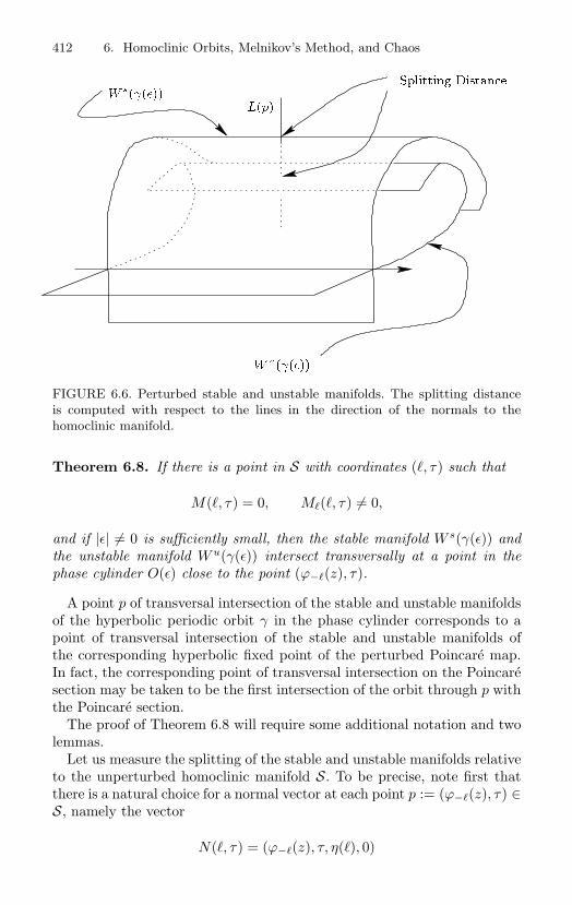
412 6. Homoclinic Orbits, Melnikov’s Method, and Chaos
Lp
Wu
Splitting DistanceW s
FIGURE 6.6. Perturbed stable and unstable manifolds. The splitting distanceis computed with respect to the lines in the direction of the normals to thehomoclinic manifold.
Theorem 6.8. If there is a point in S with coordinates (, τ) such that
M(, τ) = 0, M(, τ) = 0,
and if |ε| = 0 is sufficiently small, then the stable manifold W s(γ(ε)) andthe unstable manifold Wu(γ(ε)) intersect transversally at a point in thephase cylinder O(ε) close to the point (ϕ−(z), τ).
A point p of transversal intersection of the stable and unstable manifoldsof the hyperbolic periodic orbit γ in the phase cylinder corresponds to apoint of transversal intersection of the stable and unstable manifolds ofthe corresponding hyperbolic fixed point of the perturbed Poincare map.In fact, the corresponding point of transversal intersection on the Poincaresection may be taken to be the first intersection of the orbit through p withthe Poincare section.
The proof of Theorem 6.8 will require some additional notation and twolemmas.
Let us measure the splitting of the stable and unstable manifolds relativeto the unperturbed homoclinic manifold S. To be precise, note first thatthere is a natural choice for a normal vector at each point p := (ϕ−(z), τ) ∈S, namely the vector
N(, τ) = (ϕ−(z), τ, η(), 0)
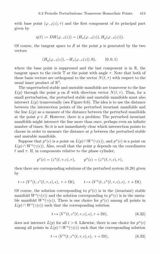
6.2 Periodic Perturbations: Transverse Homoclinic Points 413
with base point (ϕ−(z), τ) and the first component of its principal partgiven by
η() := DH(ϕ−(z)) = (Hx(ϕ−(z)), Hy(ϕ−(z))).
Of course, the tangent space to S at the point p is generated by the twovectors
(Hy(ϕ−(z)),−Hx(ϕ−(z)), 0), (0, 0, 1)
where the base point is suppressed and the last component is in R, thetangent space to the circle T at the point with angle τ . Note that both ofthese basis vectors are orthogonal to the vector N(, τ) with respect to theusual inner product of R
3.The unperturbed stable and unstable manifolds are transverse to the line
L(p) through the point p on S with direction vector N(, τ). Thus, for asmall perturbation, the perturbed stable and unstable manifolds must alsointersect L(p) transversally (see Figure 6.6). The idea is to use the distancebetween the intersection points of the perturbed invariant manifolds andthe line L(p) as a measure of the distance between the perturbed manifoldsat the point p ∈ S. However, there is a problem: The perturbed invariantmanifolds might intersect the line more than once, perhaps even an infinitenumber of times. So it is not immediately clear which intersection points tochoose in order to measure the distance at p between the perturbed stableand unstable manifolds.
Suppose that ps(ε) is a point on L(p)∩W s(γ(ε)), and pu(ε) is a point onL(p) ∩ Wu(γ(ε)). Also, recall that the point p depends on the coordinates and τ . If, in components relative to the phase cylinder,
ps(ε) = (zs(, τ, ε), τ), pu(ε) = (zu(, τ, ε), τ),
then there are corresponding solutions of the perturbed system (6.28) givenby
t → (V s(t, zs(, τ, ε), ε), τ + Ωt), t → (V u(t, zu(, τ, ε), ε), τ + Ωt).
Of course, the solution corresponding to ps(ε) is in the (invariant) stablemanifold W s(γ(ε)) and the solution corresponding to pu(ε) is in the unsta-ble manifold Wu(γ(ε)). There is one choice for ps(ε) among all points inL(p) ∩ W s(γ(ε)) such that the corresponding solution
t → (V s(t, zs(, τ, ε), ε), τ + Ωt), (6.32)
does not intersect L(p) for all t > 0. Likewise, there is one choice for pu(ε)among all points in L(p) ∩ Wu(γ(ε)) such that the corresponding solution
t → (V u(t, zu(, τ, ε), ε), τ + Ωt), (6.33)
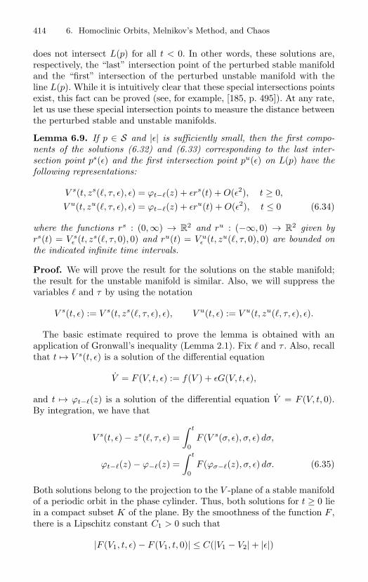
414 6. Homoclinic Orbits, Melnikov’s Method, and Chaos
does not intersect L(p) for all t < 0. In other words, these solutions are,respectively, the “last” intersection point of the perturbed stable manifoldand the “first” intersection of the perturbed unstable manifold with theline L(p). While it is intuitively clear that these special intersections pointsexist, this fact can be proved (see, for example, [185, p. 495]). At any rate,let us use these special intersection points to measure the distance betweenthe perturbed stable and unstable manifolds.
Lemma 6.9. If p ∈ S and |ε| is sufficiently small, then the first compo-nents of the solutions (6.32) and (6.33) corresponding to the last inter-section point ps(ε) and the first intersection point pu(ε) on L(p) have thefollowing representations:
V s(t, zs(, τ, ε), ε) = ϕt−(z) + εrs(t) + O(ε2), t ≥ 0,
V u(t, zu(, τ, ε), ε) = ϕt−(z) + εru(t) + O(ε2), t ≤ 0 (6.34)
where the functions rs : (0,∞) → R2 and ru : (−∞, 0) → R
2 given byrs(t) = V s
ε (t, zs(, τ, 0), 0) and ru(t) = V uε (t, zu(, τ, 0), 0) are bounded on
the indicated infinite time intervals.
Proof. We will prove the result for the solutions on the stable manifold;the result for the unstable manifold is similar. Also, we will suppress thevariables and τ by using the notation
V s(t, ε) := V s(t, zs(, τ, ε), ε), V u(t, ε) := V u(t, zu(, τ, ε), ε).
The basic estimate required to prove the lemma is obtained with anapplication of Gronwall’s inequality (Lemma 2.1). Fix and τ . Also, recallthat t → V s(t, ε) is a solution of the differential equation
V = F (V, t, ε) := f(V ) + εG(V, t, ε),
and t → ϕt−(z) is a solution of the differential equation V = F (V, t, 0).By integration, we have that
V s(t, ε) − zs(, τ, ε) =∫ t
0F (V s(σ, ε), σ, ε) dσ,
ϕt−(z) − ϕ−(z) =∫ t
0F (ϕσ−(z), σ, ε) dσ. (6.35)
Both solutions belong to the projection to the V -plane of a stable manifoldof a periodic orbit in the phase cylinder. Thus, both solutions for t ≥ 0 liein a compact subset K of the plane. By the smoothness of the function F ,there is a Lipschitz constant C1 > 0 such that
|F (V1, t, ε) − F (V1, t, 0)| ≤ C(|V1 − V2| + |ε|)
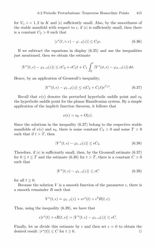
6.2 Periodic Perturbations: Transverse Homoclinic Points 415
for Vi, i = 1, 2 in K and |ε| sufficiently small. Also, by the smoothness ofthe stable manifold with respect to ε, if |ε| is sufficiently small, then thereis a constant C2 > 0 such that
|zs(, τ, ε) − ϕ−(z)| ≤ C2ε. (6.36)
If we subtract the equations in display (6.35) and use the inequalitiesjust mentioned, then we obtain the estimate
|V s(t, ε) − ϕt−(z)| ≤ εC2 + εC1t + C1
∫ t
0|V s(σ, ε) − ϕσ−(z)| dσ.
Hence, by an application of Gronwall’s inequality,
|V s(t, ε) − ϕt−(z)| ≤ ε(C2 + C1t)eC1t. (6.37)
Recall that ν(ε) denotes the perturbed hyperbolic saddle point and ν0the hyperbolic saddle point for the planar Hamiltonian system. By a simpleapplication of the implicit function theorem, it follows that
ν(ε) = ν0 + O(ε).
Since the solutions in the inequality (6.37) belong to the respective stablemanifolds of ν(ε) and ν0, there is some constant C3 > 0 and some T > 0such that if t > T , then
|V s(t, ε) − ϕt−(z)| ≤ εC3. (6.38)
Therefore, if |ε| is sufficiently small, then, by the Gronwall estimate (6.37)for 0 ≤ t ≤ T and the estimate (6.38) for t > T , there is a constant C > 0such that
|V s(t, ε) − ϕt−(z)| ≤ εC (6.39)
for all t ≥ 0.Because the solution V is a smooth function of the parameter ε, there is
a smooth remainder R such that
V s(t, ε) = ϕt−(z) + εrs(t) + ε2R(t, ε).
Thus, using the inequality (6.39), we have that
ε|rs(t) + εR(t, ε)| = |V s(t, ε) − ϕt−(z)| ≤ εC.
Finally, let us divide this estimate by ε and then set ε = 0 to obtain thedesired result: |rs(t)| ≤ C for t ≥ 0.
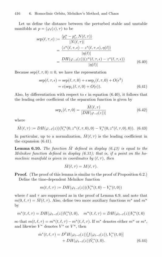
416 6. Homoclinic Orbits, Melnikov’s Method, and Chaos
Let us define the distance between the perturbed stable and unstablemanifolds at p = (ϕ(z), τ) to be
sep(, τ, ε) :=〈pu
ε − psε , N(, τ)〉
|N(, τ)|
=〈zu(, τ, ε) − zs(, τ, ε), η()〉
|η()|
=DH(ϕ−(z))(zu(, τ, ε) − zs(, τ, ε))
|η()| (6.40)
Because sep(, τ, 0) ≡ 0, we have the representation
sep(, τ, ε) = sep(, τ, 0) + ε sepε(, τ, 0) + O(ε2)= ε(sepε(, τ, 0) + O(ε)). (6.41)
Also, by differentiation with respect to ε in equation (6.40), it follows thatthe leading order coefficient of the separation function is given by
sepε(, τ, 0) =M(, τ)
|DH(ϕ−(z))| (6.42)
where
M(, τ) := DH(ϕ−(z))(V uε (0, zu(, τ, 0), 0) − V s
ε (0, zs(, τ, 0), 0)). (6.43)
In particular, up to a normalization, M(, τ) is the leading coefficient inthe expansion (6.41).
Lemma 6.10. The function M defined in display (6.43) is equal to theMelnikov function defined in display (6.31); that is, if a point on the ho-moclinic manifold is given in coordinates by (, τ), then
M(, τ) = M(, τ).
Proof. (The proof of this lemma is similar to the proof of Proposition 6.2.)Define the time-dependent Melnikov function
m(t, , τ) := DH(ϕt−(z))(V uε (t, 0) − V s
ε (t, 0))
where and τ are suppressed as in the proof of Lemma 6.9, and note thatm(0, , τ) = M(, τ). Also, define two more auxiliary functions ms and mu
by
ms(t, , τ) = DH(ϕt−(z))V sε (t, 0), mu(t, , τ) = DH(ϕt−(z))V u
ε (t, 0)
so that m(t, , τ) = mu(t, , τ)−ms(t, , τ). If m∗ denotes either mu or ms,and likewise V ∗ denotes V s or V u, then
m∗(t, , τ) = D2H(ϕt−(z))[f(ϕt−(z)), V ∗ε (t, 0)]
+ DH(ϕt−(z))V ∗ε (t, 0). (6.44)
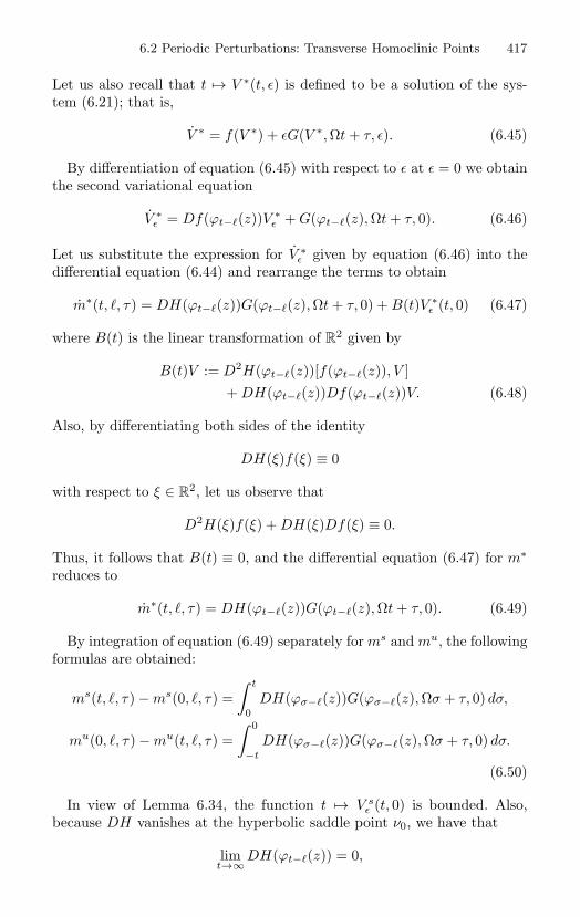
6.2 Periodic Perturbations: Transverse Homoclinic Points 417
Let us also recall that t → V ∗(t, ε) is defined to be a solution of the sys-tem (6.21); that is,
V ∗ = f(V ∗) + εG(V ∗, Ωt + τ, ε). (6.45)
By differentiation of equation (6.45) with respect to ε at ε = 0 we obtainthe second variational equation
V ∗ε = Df(ϕt−(z))V ∗
ε + G(ϕt−(z), Ωt + τ, 0). (6.46)
Let us substitute the expression for V ∗ε given by equation (6.46) into the
differential equation (6.44) and rearrange the terms to obtain
m∗(t, , τ) = DH(ϕt−(z))G(ϕt−(z), Ωt + τ, 0) + B(t)V ∗ε (t, 0) (6.47)
where B(t) is the linear transformation of R2 given by
B(t)V := D2H(ϕt−(z))[f(ϕt−(z)), V ]+ DH(ϕt−(z))Df(ϕt−(z))V. (6.48)
Also, by differentiating both sides of the identity
DH(ξ)f(ξ) ≡ 0
with respect to ξ ∈ R2, let us observe that
D2H(ξ)f(ξ) + DH(ξ)Df(ξ) ≡ 0.
Thus, it follows that B(t) ≡ 0, and the differential equation (6.47) for m∗
reduces to
m∗(t, , τ) = DH(ϕt−(z))G(ϕt−(z), Ωt + τ, 0). (6.49)
By integration of equation (6.49) separately for ms and mu, the followingformulas are obtained:
ms(t, , τ) − ms(0, , τ) =∫ t
0DH(ϕσ−(z))G(ϕσ−(z), Ωσ + τ, 0) dσ,
mu(0, , τ) − mu(t, , τ) =∫ 0
−t
DH(ϕσ−(z))G(ϕσ−(z), Ωσ + τ, 0) dσ.
(6.50)
In view of Lemma 6.34, the function t → V sε (t, 0) is bounded. Also,
because DH vanishes at the hyperbolic saddle point ν0, we have that
limt→∞ DH(ϕt−(z)) = 0,
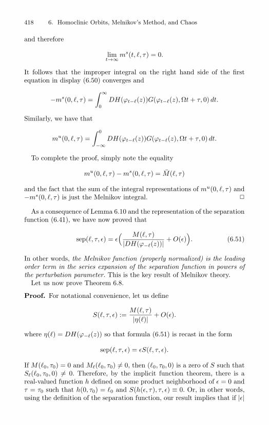
418 6. Homoclinic Orbits, Melnikov’s Method, and Chaos
and therefore
limt→∞ ms(t, , τ) = 0.
It follows that the improper integral on the right hand side of the firstequation in display (6.50) converges and
−ms(0, , τ) =∫ ∞
0DH(ϕt−(z))G(ϕt−(z), Ωt + τ, 0) dt.
Similarly, we have that
mu(0, , τ) =∫ 0
−∞DH(ϕt−(z))G(ϕt−(z), Ωt + τ, 0) dt.
To complete the proof, simply note the equality
mu(0, , τ) − ms(0, , τ) = M(, τ)
and the fact that the sum of the integral representations of mu(0, , τ) and−ms(0, , τ) is just the Melnikov integral.
As a consequence of Lemma 6.10 and the representation of the separationfunction (6.41), we have now proved that
sep(, τ, ε) = ε( M(, τ)
|DH(ϕ−(z))| + O(ε)). (6.51)
In other words, the Melnikov function (properly normalized) is the leadingorder term in the series expansion of the separation function in powers ofthe perturbation parameter. This is the key result of Melnikov theory.
Let us now prove Theorem 6.8.
Proof. For notational convenience, let us define
S(, τ, ε) :=M(, τ)|η()| + O(ε).
where η() = DH(ϕ−(z)) so that formula (6.51) is recast in the form
sep(, τ, ε) = εS(, τ, ε).
If M(0, τ0) = 0 and M(0, τ0) = 0, then (0, τ0, 0) is a zero of S such thatS(0, τ0, 0) = 0. Therefore, by the implicit function theorem, there is areal-valued function h defined on some product neighborhood of ε = 0 andτ = τ0 such that h(0, τ0) = 0 and S(h(ε, τ), τ, ε) ≡ 0. Or, in other words,using the definition of the separation function, our result implies that if |ε|
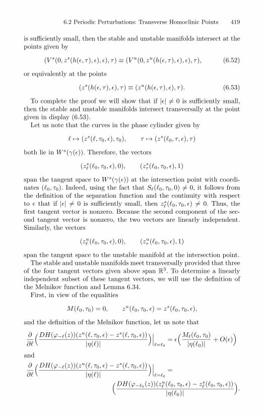
6.2 Periodic Perturbations: Transverse Homoclinic Points 419
is sufficiently small, then the stable and unstable manifolds intersect at thepoints given by
(V s(0, zs(h(ε, τ), ε), ε), τ) ≡ (V u(0, zu(h(ε, τ), ε), ε), τ), (6.52)
or equivalently at the points
(zs(h(ε, τ), ε), τ) ≡ (zu(h(ε, τ), ε), τ). (6.53)
To complete the proof we will show that if |ε| = 0 is sufficiently small,then the stable and unstable manifolds intersect transversally at the pointgiven in display (6.53).
Let us note that the curves in the phase cylinder given by
→ (zs(, τ0, ε), τ0), τ → (zs(0, τ, ε), τ)
both lie in W s(γ(ε)). Therefore, the vectors
(zs (0, τ0, ε), 0), (zs
τ (0, τ0, ε), 1)
span the tangent space to W s(γ(ε)) at the intersection point with coordi-nates (0, τ0). Indeed, using the fact that S(0, τ0, 0) = 0, it follows fromthe definition of the separation function and the continuity with respectto ε that if |ε| = 0 is sufficiently small, then zs
(0, τ0, ε) = 0. Thus, thefirst tangent vector is nonzero. Because the second component of the sec-ond tangent vector is nonzero, the two vectors are linearly independent.Similarly, the vectors
(zu (0, τ0, ε), 0), (zu
τ (0, τ0, ε), 1)
span the tangent space to the unstable manifold at the intersection point.The stable and unstable manifolds meet transversally provided that three
of the four tangent vectors given above span R3. To determine a linearly
independent subset of these tangent vectors, we will use the definition ofthe Melnikov function and Lemma 6.34.
First, in view of the equalities
M(0, τ0) = 0, zu(0, τ0, ε) = zs(0, τ0, ε),
and the definition of the Melnikov function, let us note that
∂
∂
(DH(ϕ−(z))(zu(, τ0, ε) − zs(, τ0, ε))|η()|
)∣∣∣=0
= ε(M(0, τ0)
|η(0)|+ O(ε)
)and∂
∂
(DH(ϕ−(z))(zu(, τ0, ε) − zs(, τ0, ε))|η()|
)∣∣∣=0
=(DH(ϕ−0(z))(zu (0, τ0, ε) − zs
(0, τ0, ε))|η(0)|
).
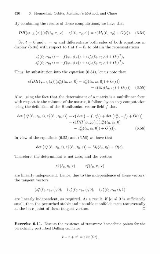
420 6. Homoclinic Orbits, Melnikov’s Method, and Chaos
By combining the results of these computations, we have that
DH(ϕ−0(z))(zu (0, τ0, ε) − zs
(0, τ0, ε)) = ε(M(0, τ0) + O(ε)). (6.54)
Set t = 0 and τ = τ0 and differentiate both sides of both equations indisplay (6.34) with respect to at = 0 to obtain the representations
zs (0, τ0, ε) = −f(ϕ−(z)) + εzs
ε(0, τ0, 0) + O(ε2),zu
(0, τ0, ε) = −f(ϕ−(z)) + εzuε(0, τ0, 0) + O(ε2).
Thus, by substitution into the equation (6.54), let us note that
ε(DH(ϕ−0(z))(zu
ε(0, τ0, 0) − zsε(0, τ0, 0)) + O(ε)
)= ε(M(0, τ0) + O(ε)). (6.55)
Also, using the fact that the determinant of a matrix is a multilinear formwith respect to the columns of the matrix, it follows by an easy computationusing the definition of the Hamiltonian vector field f that
det(zu
(0, τ0, ε), zs (0, τ0, ε)
)= ε
(det
(− f, zs
ε
)+ det
(zu
ε,−f)
+ O(ε))
= ε(DH(ϕ−0(z)(zuε(0, τ0, 0)
− zsε(0, τ0, 0)) + O(ε)). (6.56)
In view of the equations (6.55) and (6.56) we have that
det(zu
(0, τ0, ε), zs (0, τ0, ε)
)= M(0, τ0) + O(ε).
Therefore, the determinant is not zero, and the vectors
zu (0, τ0, ε), zs
(0, τ0, ε)
are linearly independent. Hence, due to the independence of these vectors,the tangent vectors
(zu (0, τ0, ε), 0), (zs
(0, τ0, ε), 0), (zsτ (0, τ0, ε), 1)
are linearly independent, as required. As a result, if |ε| = 0 is sufficientlysmall, then the perturbed stable and unstable manifolds meet transversallyat the base point of these tangent vectors.
Exercise 6.11. Discuss the existence of transverse homoclinic points for theperiodically perturbed Duffing oscillator
x − x + x3 = ε sin(Ωt).
6.3 Origins of ODE: Fluid Dynamics 421
Exercise 6.12. Discuss the existence of transverse homoclinic points for theperiodically perturbed damped pendulum
θ + ω2 sin θ = εg(θ, t)
where
g(θ, t) := −λθ + sin(Ωt).
How does the existence of transverse homoclinic points depend on the parame-ters? What happens if the sinusoidal time periodic external force is replaced bya smooth periodic function p(t). What happens if the viscous damping term isreplaced by −λθ2?
Exercise 6.13. Discuss the existence of transverse homoclinic points for theparametrically excited pendulum
θ + (ω2 + ε cos(Ωt)) sin θ = 0.
Exercise 6.14. Discuss the existence of transverse homoclinic points for thependulum with “feedback control”
θ + sin θ + αθ − β = ε(−λθ + γ cos(Ωt)
(see [188]). The “Melnikov analysis” of this system seems to require numericalapproximations of the Melnikov integral. Compute an approximation of the Mel-nikov integral and find parameter values where your computations suggest theexistence of simple zeros. Plot some orbits of the stroboscopic Poincare map toobtain an approximation of its phase portrait. Also find parameter values where anumerical experiment suggests the corresponding dynamical system has sensitivedependence on initial conditions.
Exercise 6.15. Using formula (6.31), prove that M(, τ) = 0 if and only ifMτ (, τ) = 0. Note that a corollary of this result is the conclusion of Theorem 6.8under the hypothesis that M(, τ) = 0 and Mτ (, τ) = 0.
6.3 Origins of ODE: Fluid Dynamics
The description of the motion of fluids is a central topic in practical scien-tific research with a vast literature in physics, engineering, mathematics,and computation. The basic model is a system of partial differential equa-tions of evolution type. Thus, as might be expected, many specializations ofthis model lead to ordinary differential equations. In fact, some of the mostinteresting and most important problems in ordinary differential equationshave their origin in fluid dynamics.
The purpose of this section is to briefly discuss the Euler and Navier–Stokes model equations; to derive a system of ordinary differential equa-tions, called the ABC system, that has been used to describe the steadystate motion of an ideal fluid in a certain ideal situation; and to discuss thedynamics of the ABC system as an application of our analysis of perturbedoscillators.
Caution: Treat this section as “a finger pointing at the moon.”
422 6. Homoclinic Orbits, Melnikov’s Method, and Chaos
6.3.1 The Equations of Fluid MotionLet us consider a fluid with constant density ρ confined to some regionR in space, and let us assume that the motion of the fluid is given bythe time-dependent velocity field u : R × R → R
3 with (ξ, t) → u(ξ, t).The position of a particle of the moving fluid is given by a smooth curvet → γ(t) in R. Thus, the momentum of this fluid particle is ρu(γ(t), t),and, according to Newton’s law, the motion of the particle is given by thedifferential equation
ρd
dt(u(γ(t), t)) = F
where F denotes the sum of the forces. Of course, a fluid is always subjectedto the force of gravity and perhaps to other external body forces. However,let us ignore these forces and consider only the constitutive force laws thatmodel the internal shear forces that are essential to our understanding ofthe physical nature of fluids, just as Hooke’s law is the essential constitutiveforce law for springs.
Internal fluid forces can be derived from more basic physical laws (see,for example, [48] and [105]); however, let us simply note that the basic forcelaw is
F = µ∆u − gradP
where µ is a constant related to the viscosity of the fluid, P is called the fluidpressure, and the Laplacian operates on the velocity field componentwise.Of course, the gradient and the Laplacian derivatives are with respect to thespace variables only. Let us also note that the viscosity term is a function ofthe fluid velocity, but the pressure is a second unknown dependent variablein the system. Thus, we will have to have two equations in the two unknownfunctions u and P .
Using Newton’s law and the constitutive force law, the equation of motionfor a fluid is
ρ(∂u
∂t(ξ, t) + Du(ξ, t)u(ξ, t)
)= µ∆u(ξ, t) − gradP (ξ, t)
where D denotes differentiation with respect to the space variables. Influid mechanics, if x, y, z are the Cartesian coordinates in R
3 and ex, ey, ez
are the usual unit direction vectors (here the subscripts denote coordinatedirections, not partial derivatives), then the gradient operator
∇ :=∂
∂xex +
∂
∂yey +
∂
∂zez
is introduced and the advection term (Du)u is rewritten, using the usualinner product, in the form 〈u, ∇〉u, or more commonly as u · ∇u. Here, ∇acts componentwise on the vector field u.
6.3 Origins of ODE: Fluid Dynamics 423
The fluid density must satisfy the continuity equation (3.81)
∂ρ
∂t+ div(ρu) = 0.
Thus, under our assumption that the density is constant (homogeneousfluid), we must have that u is divergence free. This is equivalent to theassumption that the fluid is incompressible.
Because our fluid is confined to a region of space, some boundary condi-tions must be imposed. In fact, physical experiments show that the correctboundary condition is u ≡ 0 on the boundary ∂R of the region R. Todemonstrate this fact yourself, consider cleaning a metal plate by using ahose to spray it with water; for example, try cleaning a dirty automobile.As the pressure of the water increases, the size of the particles of dirt thatcan be removed decreases. However, it is very difficult to remove all thedirt by spraying alone. This can be checked by polishing with a cloth. Infact, the velocity of the spray decreases rapidly in the boundary layer nearthe plate. Dirt particles with sufficiently small diameter are not subjectedto flow velocities that are high enough to dislodge them.
If units of length and velocity are introduced, then the system of equa-tions for the velocity field and the pressure can be rescaled to the dimen-sionless form of the Navier–Stokes equations for an incompressible fluid inR given by
∂u
∂t+ u · ∇u =
1Re
∆ − grad p,
div u = 0,
u = 0 in ∂R (6.57)
where Re, the Reynolds number, is given by length multiplied by velocitydivided by viscosity. The existence of this scaling is important: If two flowshave the same Reynold’s number, then the flows have the same dynamics.For example, flow around a scaled model of an airplane in a wind tunnelmight be tested at the same Reynold’s number expected for the airplaneunder certain flight conditions. Perhaps the same Reynold’s number canbe obtained by increasing the velocity in the wind tunnel to compensatefor the smaller length scale of the model. In principle, the behavior of themodel is then exactly the same as the real aircraft.
Euler’s equations for fluid motion can be viewed as an idealization of theNavier–Stokes equations for a fluid with zero viscosity. These equationshave the form
∂u
∂t+ u · ∇u = − grad p,
div u = 0,
〈u, η〉 = 0 in ∂R (6.58)
424 6. Homoclinic Orbits, Melnikov’s Method, and Chaos
where η is the outward unit normal vector field on ∂R. Note that the “noslip” boundary condition for the Navier–Stokes equations is replaced by thecondition that there is no fluid passing through the boundary. The reasonfor the physically unrealistic Euler boundary conditions is to ensure thatEuler’s partial differential equations are “well posed”, that is, they haveunique solutions depending continuously on initial conditions.
A naive expectation is that the limit of a family of solutions of theNavier–Stokes equations as the Reynold’s number increases without boundis a solution of Euler’s equations. After all, the term ∆u/Re would seemto go to zero as Re → ∞. However, it is also possible that the secondderivatives of the velocity field are unbounded in the limit. For this andother reasons, the limiting behavior of the Navier–Stokes equations for largevalues of the Reynold’s number is not yet completely understood. Thus, thedynamical behavior of the family as the Reynold’s number grows withoutbound is a fruitful area of research.
Flow in A Pipe
As an example of the solution of a fluid flow problem, let us consider per-haps the most basic example of the subject: flow in a round pipe.
If we choose cylindrical coordinates r, θ, z with the z-axis being the axisof symmetry of a round pipe with radius a, then it seems natural to expectthat there are some flow regimes for which the velocity field has its onlynonzero component in the axial direction of the pipe; that is, the velocityfield has the form
u(r, θ, z, t) = (0, 0, uz(r, θ, z, t)) (6.59)
where the components are with respect to the basis vector fields er, eθ, ez
that are defined in terms of the usual basis of Euclidean space by
er := (cos θ, sin θ, 0), eθ := (− sin θ, cos θ, 0), ez := (0, 0, 1).
Let us express the Euler and the Navier–Stokes equations in cylindricalcoordinates. Recall that if f is a function and F = Frer + Fθeθ + Fzez is avector field on Euclidean space, then in cylindrical coordinates,
∇f =∂f
∂rer +
1r
∂f
∂θeθ +
∂f
∂zez,
div f =1r
∂
∂r(rFr) +
1r
∂Fθ
∂θ+
∂Fz
∂z,
∆f =1r
∂
∂r
(r∂f
∂θ
)+
1r2
∂2f
∂r2 +∂2f
∂z2 . (6.60)
To obtain the Navier–Stokes equations in cylindrical coordinates, considerthe unknown velocity field u = urer + uθeθ + uzez. Write this vector
6.3 Origins of ODE: Fluid Dynamics 425
field in the usual Cartesian components by using the definitions of thedirection fields given above, insert the result into the Navier–Stokes equa-tions, and then compute the space derivatives using the operators givenin display (6.60). If we multiply the first two of the resulting componentequations—the equations in the directions ex and ey—by the matrix(
cos θ sin θ− sin θ cos θ
),
then we obtain the equivalent system
∂ur
∂t+ (u · ∇)ur − 1
ru2
θ =1
Re(∆ur − 1
r2 (ur + 2∂uθ
∂θ))
− ∂p
∂r,
∂uθ
∂t+ (u · ∇)uθ +
1ruruθ =
1Re
(∆uθ − 1
r2 (uθ − 2∂ur
∂θ))
− 1r
∂p
∂θ,
∂uz
∂t+ (u · ∇)uz =
1Re
∆uz − ∂p
∂z,
div u = 0. (6.61)
The Euler equations in cylindrical coordinates for the fluid motion in thepipe are obtained from system (6.61) by deleting the terms that are dividedby the Reynold’s number. If the velocity field u has the form given inequation (6.59), then u automatically satisfies the Euler boundary conditionat the wall of the pipe. Thus, the Euler equations for the velocity field uand the scaled pressure p reduce to the system
∂p
∂r= 0,
∂p
∂θ= 0,
∂uz
∂t+ uz
∂uz
∂z= −∂p
∂z= 0,
∂uz
∂z= 0.
It follows that p must be a function of z only, and
∂uz
∂t= −∂p
∂z. (6.62)
If we now differentiate equation (6.62) with respect to z, then we see im-mediately that ∂2p/∂z2 = 0. Therefore, p = p0 + p1z for some constants p0and p1, and we must also have that uz = −p1t + u0 for some constant u0.Let us note that if we were to impose the no slip boundary conditions, thenthe only possible solution is uz = 0 and p = p0. Thus, a nonzero initialfluid velocity cannot be imposed.
There are two cases for the Euler flow: If p1 = 0, then the pressure isconstant in the pipe and the velocity field is constant. This is called plugflow. If p1 = 0, then both the pressure and the velocity become unboundedas time passes to infinity. Both cases are not physically realistic. For exam-ple, the first case does not satisfy the experimentally observed fact that thevelocity of the flow approaches zero at the wall of the pipe. Nonetheless, be-cause of its mathematical simplicity, plug flow is often used as a model. For
426 6. Homoclinic Orbits, Melnikov’s Method, and Chaos
example, plug flow is often used to model flow in tubular reactors studiedin chemical engineering.
What about Navier–Stokes flow?If we consider the same pipe, the same coordinate system, and the same
hypothesis about the direction of the velocity field, then the Navier–Stokesequations reduce to
∂p
∂r= 0,
∂p
∂θ= 0,
∂uz
∂t+ uz
∂uz
∂z=
1Re
∆uz − ∂p
∂z= 0,
∂uz
∂z= 0,
with the no slip boundary condition at the wall of the pipe given by
uz(a, θ, z, t) ≡ 0.
This system of equations is already difficult to solve! However, we canobtain a solution if we make two additional assumptions: The velocity fieldis in steady state and it is symmetric with respect to rotations about thecentral axis of the pipe. With these assumptions, if we take into accountthe equation ∂uz/∂z = 0, then it suffices to solve the single equation
1Re
(1r
∂
∂r
(r∂uz
∂r
))= pz.
Because pr and pθ must be constant, we have that pz depends only on zwhile the left hand side of the last equation depends only on r. Thus, thefunctions on both sides of the equation must have the same constant value,say c. If this is the case, then p = cz + p0.
The remaining ordinary differential equation
ru′′z (r) + u′
z(r) = (cRe)r
with the initial condition uz(a) = 0 has the continuous solution
uz(r) =14cRe (r2 − a2).
Thus, we have derived the result that the steady state velocity field u pre-dicted by the Navier–Stokes equations is parabolic with respect to the radialcoordinate. This flow field is physically realistic, at least if the Reynold’snumber is sufficiently small; it is called Poiseuille flow.
Exercise 6.16. Consider Poiseuille flow in a section of length L of an infiniteround pipe with radius a. If the pressure is p in at the inlet of the section andthe flow speed at the center of the pipe is v in, then determine the pressure atthe outlet. What happens in the limit as the Reynold’s number grows withoutbound? Compare with the prediction of plug flow.
6.3 Origins of ODE: Fluid Dynamics 427
Using the vector identity
12
grad(u · u) = u × curlu + u · ∇u
where · denotes the usual inner product on Euclidean space, let us rewriteEuler’s equation in the form
ut − u × curlu = grad(−12(u · u) − p).
If we now define α := − 12 |u|2−p, then we obtain Bernoulli’s form of Euler’s
equations
ut = u × curlu + gradα,
div u = 0,
u · η = 0 in ∂R. (6.63)
Potential Flow
Let us consider an important specialization of Bernoulli’s form of Euler’sequations: potential flow in two space dimensions. The idea is the following.Assume that the velocity field u is the gradient of a potential f so that u =grad f . Substitution into system (6.63) using the fact that curl(gradu) = 0and some rearrangement gives the equations of motion
grad(∂f
∂t+
12| grad f |2 − p) = 0, ∆f = 0. (6.64)
As a result, we see immediately that the quantity
∂f
∂t+
12| grad f |2 − p
is constant with respect to the space variables. In particular, if u is a steadystate velocity field, then there is a constant c such that
p = c − 12|u|2; (6.65)
that is, the pressure is a constant minus half the square of the velocity.This is Bernoulli’s law.
In view of the second equation of system (6.64), the potential f is aharmonic function. Therefore, in the plane with Cartesian coordinates x, ywhere the velocity field is given by u = (x, y), the potential f is locally thereal part of a holomorphic function, say h = f + iψ. Moreover, the pairf, ψ satisfies the Cauchy–Riemann equations
∂f
∂x=
∂ψ
∂y,
∂f
∂y= −∂ψ
∂x.
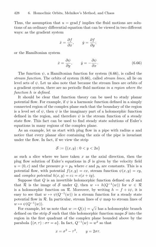
428 6. Homoclinic Orbits, Melnikov’s Method, and Chaos
Thus, the assumption that u = grad f implies the fluid motions are solu-tions of an ordinary differential equation that can be viewed in two differentways: as the gradient system
x =∂f
∂x, y =
∂f
∂y;
or the Hamiltonian system
x =∂ψ
∂y, y = −∂ψ
∂x. (6.66)
The function ψ, a Hamiltonian function for system (6.66), is called thestream function. The orbits of system (6.66), called stream lines, all lie onlevel sets of ψ. Let us also note that because the stream lines are orbits ofa gradient system, there are no periodic fluid motions in a region where thefunction h is defined.
It should be clear that function theory can be used to study planarpotential flow. For example, if ψ is a harmonic function defined in a simplyconnected region of the complex plane such that the boundary of the regionis a level set of ψ, then ψ is the imaginary part of a holomorphic functiondefined in the region, and therefore ψ is the stream function of a steadystate flow. This fact can be used to find steady state solutions of Euler’sequations in many regions of the complex plane.
As an example, let us start with plug flow in a pipe with radius a andnotice that every planar slice containing the axis of the pipe is invariantunder the flow. In fact, if we view the strip
S := (x, y) : 0 < y < 2a
as such a slice where we have taken x as the axial direction, then theplug flow solution of Euler’s equations in S is given by the velocity fieldu = (0, c) and the pressure p = p0 where c and p0 are constants. This is apotential flow, with potential f(x, y) = cx, stream function ψ(x, y) = cy,and complex potential h(x, y) = cz = c(x + iy).
Suppose that Q is an invertible holomorphic function defined on S andthat R is the image of S under Q, then w → h(Q−1(w)) for w ∈ Ris a holomorphic function on R. Moreover, by writing h = f + iψ, it iseasy to see that w → ψ(Q−1(w)) is a stream function for a steady statepotential flow in R. In particular, stream lines of ψ map to stream lines ofw → ψ(Q−1(w)).
For example, let us note that w := Q(z) =√
z has a holomorphic branchdefined on the strip S such that this holomorphic function maps S into theregion in the first quadrant of the complex plane bounded above by theparabola (σ, τ) : στ = a. In fact, Q−1(w) = w2 so that
x = σ2 − τ2, y = 2στ.
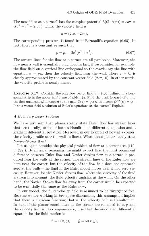
6.3 Origins of ODE: Fluid Dynamics 429
The new “flow at a corner” has the complex potential h(Q−1(w)) = cw2 =c(σ2 − τ2 + 2iστ). Thus, the velocity field is
u = (2cσ, −2cτ).
The corresponding pressure is found from Bernoulli’s equation (6.65). Infact, there is a constant p1 such that
p = p1 − 2c2(σ2 + τ2). (6.67)
The stream lines for the flow at a corner are all parabolas. Moreover, theflow near a wall is essentially plug flow. In fact, if we consider, for example,the flow field on a vertical line orthogonal to the σ-axis, say the line withequation σ = σ0, then the velocity field near the wall, where τ ≈ 0, isclosely approximated by the constant vector field (2cσ0, 0). In other words,the velocity profile is nearly linear.
Exercise 6.17. Consider the plug flow vector field u = (c, 0) defined in a hori-zontal strip in the upper half plane of width 2a. Find the push forward of u intothe first quadrant with respect to the map Q(z) =
√z with inverse Q−1(w) = w2.
Is this vector field a solution of Euler’s equations at the corner? Explain.
A Boundary Layer Problem
We have just seen that planar steady state Euler flow has stream linesthat are (locally) orbits of both a Hamiltonian differential equation and agradient differential equation. Moreover, in our example of flow at a corner,the velocity profile near the walls is linear. What about planar steady stateNavier–Stokes flow?
Let us again consider the physical problem of flow at a corner (see [119,p. 222]). By physical reasoning, we might expect that the most prominentdifference between Euler flow and Navier–Stokes flow at a corner is pro-duced near the walls at the corner. The stream lines of the Euler flow arebent near the corner, but the velocity of the flow field does not approachzero at the walls—the fluid in the Euler model moves as if it had zero vis-cosity. However, for the Navier–Stokes flow, where the viscosity of the fluidis taken into account, the fluid velocity vanishes at the walls. On the otherhand, the Navier–Stokes flow far away from the corner would be expectedto be essentially the same as the Euler flow.
In our model, the fluid velocity field is assumed to be divergence free.Because we are working in two space dimensions, this assumption impliesthat there is a stream function; that is, the velocity field is Hamiltonian.In fact, if the planar coordinates at the corner are renamed to x, y andthe velocity field u has components v, w so that the associated differentialequation for the fluid motion is
x = v(x, y), y = w(x, y),
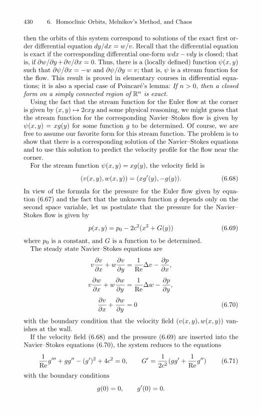
430 6. Homoclinic Orbits, Melnikov’s Method, and Chaos
then the orbits of this system correspond to solutions of the exact first or-der differential equation dy/dx = w/v. Recall that the differential equationis exact if the corresponding differential one-form wdx−vdy is closed; thatis, if ∂w/∂y+∂v/∂x = 0. Thus, there is a (locally defined) function ψ(x, y)such that ∂ψ/∂x = −w and ∂ψ/∂y = v; that is, ψ is a stream function forthe flow. This result is proved in elementary courses in differential equa-tions; it is also a special case of Poincare’s lemma: If n > 0, then a closedform on a simply connected region of R
n is exact.Using the fact that the stream function for the Euler flow at the corner
is given by (x, y) → 2cxy and some physical reasoning, we might guess thatthe stream function for the corresponding Navier–Stokes flow is given byψ(x, y) = xg(y) for some function g to be determined. Of course, we arefree to assume our favorite form for this stream function. The problem is toshow that there is a corresponding solution of the Navier–Stokes equationsand to use this solution to predict the velocity profile for the flow near thecorner.
For the stream function ψ(x, y) = xg(y), the velocity field is
(v(x, y), w(x, y)) = (xg′(y),−g(y)). (6.68)
In view of the formula for the pressure for the Euler flow given by equa-tion (6.67) and the fact that the unknown function g depends only on thesecond space variable, let us postulate that the pressure for the Navier–Stokes flow is given by
p(x, y) = p0 − 2c2(x2 + G(y)) (6.69)
where p0 is a constant, and G is a function to be determined.The steady state Navier–Stokes equations are
v∂v
∂x+ w
∂v
∂y=
1Re
∆v − ∂p
∂x,
v∂w
∂x+ w
∂w
∂y=
1Re
∆w − ∂p
∂y,
∂v
∂x+
∂w
∂y= 0 (6.70)
with the boundary condition that the velocity field (v(x, y), w(x, y)) van-ishes at the wall.
If the velocity field (6.68) and the pressure (6.69) are inserted into theNavier–Stokes equations (6.70), the system reduces to the equations
1Re
g′′′ + gg′′ − (g′)2 + 4c2 = 0, G′ =1
2c2 (gg′ +1
Reg′′) (6.71)
with the boundary conditions
g(0) = 0, g′(0) = 0.
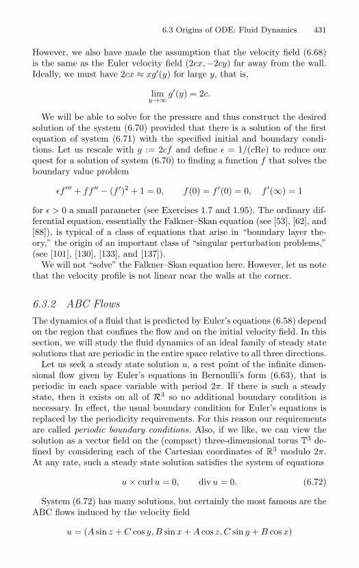
6.3 Origins of ODE: Fluid Dynamics 431
However, we also have made the assumption that the velocity field (6.68)is the same as the Euler velocity field (2cx,−2cy) far away from the wall.Ideally, we must have 2cx ≈ xg′(y) for large y, that is,
limy→∞ g′(y) = 2c.
We will be able to solve for the pressure and thus construct the desiredsolution of the system (6.70) provided that there is a solution of the firstequation of system (6.71) with the specified initial and boundary condi-tions. Let us rescale with g := 2cf and define ε = 1/(cRe) to reduce ourquest for a solution of system (6.70) to finding a function f that solves theboundary value problem
εf ′′′ + ff ′′ − (f ′)2 + 1 = 0, f(0) = f ′(0) = 0, f ′(∞) = 1
for ε > 0 a small parameter (see Exercises 1.7 and 1.95). The ordinary dif-ferential equation, essentially the Falkner–Skan equation (see [53], [62], and[88]), is typical of a class of equations that arise in “boundary layer the-ory,” the origin of an important class of “singular perturbation problems,”(see [101], [130], [133], and [137]).
We will not “solve” the Falkner–Skan equation here. However, let us notethat the velocity profile is not linear near the walls at the corner.
6.3.2 ABC FlowsThe dynamics of a fluid that is predicted by Euler’s equations (6.58) dependon the region that confines the flow and on the initial velocity field. In thissection, we will study the fluid dynamics of an ideal family of steady statesolutions that are periodic in the entire space relative to all three directions.
Let us seek a steady state solution u, a rest point of the infinite dimen-sional flow given by Euler’s equations in Bernoulli’s form (6.63), that isperiodic in each space variable with period 2π. If there is such a steadystate, then it exists on all of R3 so no additional boundary condition isnecessary. In effect, the usual boundary condition for Euler’s equations isreplaced by the periodicity requirements. For this reason our requirementsare called periodic boundary conditions. Also, if we like, we can view thesolution as a vector field on the (compact) three-dimensional torus T
3 de-fined by considering each of the Cartesian coordinates of R
3 modulo 2π.At any rate, such a steady state solution satisfies the system of equations
u × curlu = 0, div u = 0. (6.72)
System (6.72) has many solutions, but certainly the most famous are theABC flows induced by the velocity field
u = (A sin z + C cos y, B sin x + A cos z, C sin y + B cos x)
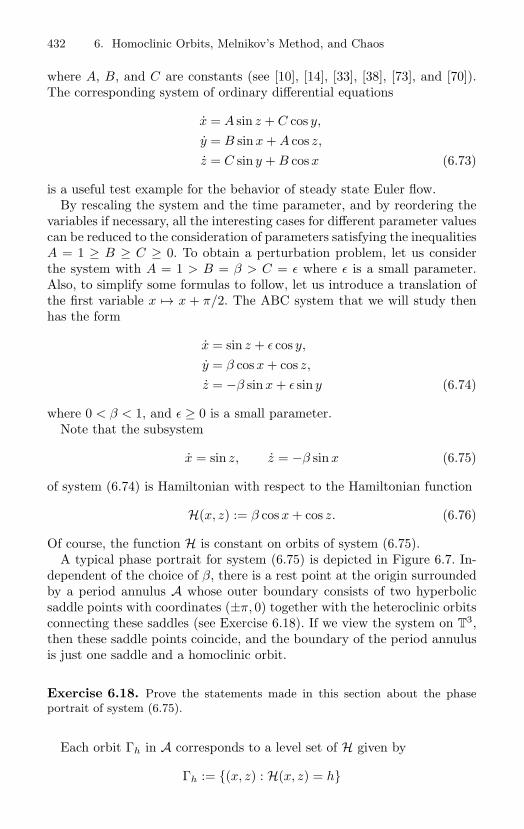
432 6. Homoclinic Orbits, Melnikov’s Method, and Chaos
where A, B, and C are constants (see [10], [14], [33], [38], [73], and [70]).The corresponding system of ordinary differential equations
x = A sin z + C cos y,
y = B sin x + A cos z,
z = C sin y + B cos x (6.73)
is a useful test example for the behavior of steady state Euler flow.By rescaling the system and the time parameter, and by reordering the
variables if necessary, all the interesting cases for different parameter valuescan be reduced to the consideration of parameters satisfying the inequalitiesA = 1 ≥ B ≥ C ≥ 0. To obtain a perturbation problem, let us considerthe system with A = 1 > B = β > C = ε where ε is a small parameter.Also, to simplify some formulas to follow, let us introduce a translation ofthe first variable x → x + π/2. The ABC system that we will study thenhas the form
x = sin z + ε cos y,
y = β cos x + cos z,
z = −β sin x + ε sin y (6.74)
where 0 < β < 1, and ε ≥ 0 is a small parameter.Note that the subsystem
x = sin z, z = −β sin x (6.75)
of system (6.74) is Hamiltonian with respect to the Hamiltonian function
H(x, z) := β cos x + cos z. (6.76)
Of course, the function H is constant on orbits of system (6.75).A typical phase portrait for system (6.75) is depicted in Figure 6.7. In-
dependent of the choice of β, there is a rest point at the origin surroundedby a period annulus A whose outer boundary consists of two hyperbolicsaddle points with coordinates (±π, 0) together with the heteroclinic orbitsconnecting these saddles (see Exercise 6.18). If we view the system on T
3,then these saddle points coincide, and the boundary of the period annulusis just one saddle and a homoclinic orbit.
Exercise 6.18. Prove the statements made in this section about the phaseportrait of system (6.75).
Each orbit Γh in A corresponds to a level set of H given by
Γh := (x, z) : H(x, z) = h
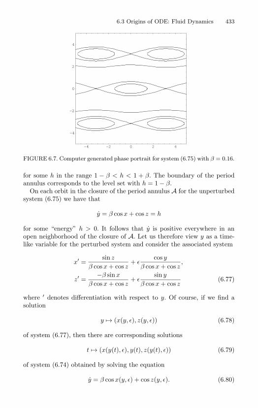
6.3 Origins of ODE: Fluid Dynamics 433
-4 -2 0 2 4
-4
-2
0
2
4
FIGURE 6.7. Computer generated phase portrait for system (6.75) with β = 0.16.
for some h in the range 1 − β < h < 1 + β. The boundary of the periodannulus corresponds to the level set with h = 1 − β.
On each orbit in the closure of the period annulus A for the unperturbedsystem (6.75) we have that
y = β cos x + cos z = h
for some “energy” h > 0. It follows that y is positive everywhere in anopen neighborhood of the closure of A. Let us therefore view y as a time-like variable for the perturbed system and consider the associated system
x′ =sin z
β cos x + cos z+ ε
cos y
β cos x + cos z,
z′ =−β sin x
β cos x + cos z+ ε
sin y
β cos x + cos z(6.77)
where ′ denotes differentiation with respect to y. Of course, if we find asolution
y → (x(y, ε), z(y, ε)) (6.78)
of system (6.77), then there are corresponding solutions
t → (x(y(t), ε), y(t), z(y(t), ε)) (6.79)
of system (6.74) obtained by solving the equation
y = β cos x(y, ε) + cos z(y, ε). (6.80)
434 6. Homoclinic Orbits, Melnikov’s Method, and Chaos
Let us notice that system (6.77) with ε = 0 is the same as system (6.75)up to a reparametrization of the independent variable. Moreover, the un-perturbed system (6.77) is a Hamiltonian system with respect to the Hamil-tonian function (6.76). Finally, we have the following useful proposition: Ify → (x(y), z(y)) is the solution of the unperturbed system (6.77) with theinitial condition x(0) = 0, z(0) = z0, then
−x(−y) = x(y), z(−y) = z(y), (6.81)
that is, x is odd and z is even. To see this, consider the new functions uand v defined by
(u(y), v(y)) = (−x(−y), z(−y))
and verify that the function y → ((u(y), v(y)) is a solution of the unper-turbed system (6.77) with the initial condition u(0) = 0, v(0) = z0.
6.3.3 Chaotic ABC FlowsThe unperturbed system (6.77) has heteroclinic cycles. For example, a cycleis formed by the hyperbolic saddle points at (x, z) = (±π, 0) and theirconnecting orbits. (Note that this cycle is also the boundary of a periodannulus.) Or, if we view the system on the phase cylinder obtained byconsidering the variable x as an angle, then this cycle has only one saddlepoint and it is connected by two distinct homoclinic orbits. In this sectionwe will see that for all but one value of the parameter β in the interval0 < β < 1, the Melnikov function along these heteroclinic orbits has simplezeros. Thus, for sufficiently small ε > 0, system (6.77), and of course thecorresponding original ABC system, has a chaotic invariant set. This resultserves as an interesting application of our perturbation theory. It suggeststhat “real” fluids have chaotic motions.
Let us recall that the unperturbed heteroclinic orbits lie on the set
(x, z) : cos z + β cos x = 1 − β, (6.82)
and let us consider the unperturbed solution y → (x(y), z(y)) startingat the point (0, arccos(1 − 2β)). The Melnikov function is given (up to anonzero scalar multiple) by
M(φ) =1
(1 − β)2
∫ ∞
−∞(sin(z(y + φ)) sin y + β sin(x(y + φ)) cos y) dy.
(6.83)
However, the integral is easily transformed to the more useful representa-tion
M(φ) =sin φ
(1 − β)2
∫ ∞
−∞(β sin x(s) sin s − sin z(s) cos s) ds (6.84)
6.3 Origins of ODE: Fluid Dynamics 435
by first changing the independent variable in the integral (6.83) to s := y+θand then by using the sum formulas for sine and cosine together with thefacts that the function y → sin x(y) is odd and y → sin z(y) is even. If, inaddition, we apply integration by parts to obtain the formula∫ ∞
−∞sin z(s) cos s ds =
β
1 − β
∫ ∞
−∞cos z(s) sin x(s) sin s ds,
and substitute for cos z(s) from the energy relation in display (6.82), thenwe have the identity∫ ∞
−∞sin z(s) cos s ds =
∫ ∞
−∞β sin x(s) sin s ds
− β2
1 − β
∫ ∞
−∞sin x(s) cos x(s) sin s ds.
Finally, by substitution of this identity into equation (6.84), we obtain thefollowing representation for the Melnikov function
M(φ) =β2 sin φ
(1 − β)3
∫ ∞
−∞sin x(s) cos x(s) sin s ds. (6.85)
Of course it is now obvious that the Melnikov function will have infinitelymany simple zeros along the heteroclinic orbit provided that the integral
Is :=∫ ∞
−∞sin x(s) cos x(s) sin s ds.
does not vanish.To determine if Is is not zero, let us consider a method to evaluate
this improper integral. The first step is to find explicit formulas for theunperturbed solution. Note that z(y) > 0 along the heteroclinic orbit.Integrate the unperturbed differential equation
x′(y)sin z(y)
=1
1 − β
on the interval (0, y), and use the energy relation to obtain the equation
y
1 − β=
∫ x(y)
0
1√1 − ((1 − β) − β cos s)2
ds
=1β
∫ x(y)
0
1√(1 + cos s)((2 − β(1 + cos s))
ds.
The form of the last integrand suggests the substitution u = 1 + cos s,which transforms the integral so that the last equality becomes
y√
β
1 − β= −
∫ 1+cos x(τ)
2
1u√
(2 − u)(2 − βu)du.
436 6. Homoclinic Orbits, Melnikov’s Method, and Chaos
Using the indefinite integral∫1
u√
(2 − u)(2 − βu)du = −1
2ln
(4√
(2 − u)(2 − βu) − 2(β + 1)u + 8u
)and a simple algebraic computation, we have the equality
cos x(y) = − (β − 1)e4cy + 2(3 − β)e2cy + β − 1(β − 1)e4cy − 2(β + 1)e2cy + β − 1
where
c :=√
β
1 − β.
Also, by the trigonometric identity sin2 x + cos2 x = 1, we have that
sin x(y) = −4√
1 − βecy(ecy − 1)
(β − 1)e4cy − 2(β + 1)e2cy + β − 1.
Define
F (w) := −4(1 − β)−3/2 w(w2 − 1)((1 − β)w4 + 2(β − 3)w2 + 1 − β)(w4 + 2 1+β
1−β w2 + 1)2
and note that
Is =∫ ∞
−∞F (ecy) sin y dy
=∫ ∞
−∞F (eζ
√β) sin((1 − β)ζ) dζ.
Also, note that the poles of the integrand of Is correspond to the zeros of thedenominator of F . To determine these zeros let us write the denominatorin the factored form
w4 + 21 + β
1 − βw2 + 1 = (w2 − u1)(w2 − u2)
where
u1 :=√
β − 1√β + 1
, u2 :=√
β + 1√β − 1
.
The poles corresponding to e2ζ√
β = u1 are
ζ =1
2√
β
(ln(−u1) + πi + 2kπi
), k ∈ Z,
6.3 Origins of ODE: Fluid Dynamics 437
where Z denotes the set of integers, and the poles corresponding to u2 are
ζ =1
2√
β
(ln(−u2) − πi + 2kπi
), k ∈ Z.
The locations of the poles suggest integration around the rectangle Γ inthe complex plane whose vertices are T , T + iπ/
√β, −T + iπ/
√β, and
−T . In fact, for sufficiently large T > 0, Γ encloses exactly two poles of theintegrand, namely,
ζ1 :=1
2√
β
(ln(−u1) + πi
), ζ2 :=
12√
β
(ln(−u2) + πi
).
The function F defined above is odd. It also has the following property:If w = 0, then F (1/w) = −F (w). Using these facts, the identity sin ζ =(eiζ − e−iζ)/(2i), and a calculation, our integral can be recast in the form
Is = −i
∫ ∞
−∞F(eζ
√β)ei(1−β)ζ dζ.
For notational convenience, define
K := K(β) =(1 − β)π
2√
β,
and also consider the contour integral∫Γ
F(eζ
√β)ei(1−β)ζ dζ.
The corresponding path integral along the upper edge of Γ is just e−2K
multiplied by the path integral along the lower edge. Also, by using theusual estimates for the absolute value of an integral, it is easy to see thatthe path integrals along the vertical edges of Γ approach zero as T increaseswithout bound. Thus, the real improper integral Is is given by
Is = −i(1 + e−2K)−1
∫Γ
F(eζ
√β)ei(1−β)ζ dζ
= 2π(1 + e−2K)−1(Res(ζ1) + Res(ζ2)) (6.86)
where the residues are computed relative to the function G given by
G(ζ) := F(eζ
√β)ei(1−β)ζ .
Define
F1(w) := (w2 − u1)2F (w), F2(w) := (w2 − u2)2F (w)
438 6. Homoclinic Orbits, Melnikov’s Method, and Chaos
and compute the Laurent series of G at ζ1 and ζ2 to obtain the followingresidues:
Res(ζ1) =ei(1−β)ζ1
4βu21
(√βeζ1
√βF ′
1(eζ1
√β)
−(2√
β − i(1 − β))F1
(eζ1
√β))
,
Res(ζ2) =ei(1−β)ζ2
4βu22
(√βeζ2
√βF ′
2(eζ2
√β)
−(2√
β − i(1 − β))F2
(eζ2
√β))
.
To simplify the sum of the residues, let us define
A := cos(1 − β
2√
βln(−u2)
), B := sin
(1 − β
2√
βln(−u2)
)so that
ei(1−β)ζ1 = e−K(A − Bi), ei(1−β)ζ2 = e−K(A + Bi),
and let us note that since u1 = 1/u2, we have
eζ1√
βeζ2√
β = −1.
Also, note that the function F1 is odd, F ′1 is even, and verify the following
identities:
F1(1/w) = − 1w4u2
2F2(w),
F ′1(1/w) =
1w2u2
2F ′
2(w) − 4w3u2
2F2(w).
Finally, for notational convenience, define L :=√
−u2 .Using the notation and the identities just mentioned, the residues are
given by
Res(ζ1) =e−K
4βu22
((A − Bi)(−iL
√β F ′
2(iL) +(2√
β + i(1 − β))F2(iL)
),
Res(ζ2) =e−K
4βu22
((A + Bi)(iL
√β F ′
2(iL) −(2√
β − i(1 − β))F2(iL)
).
Thus, in view of formula (6.86), we have
Is =πe−K
βu22(1 + e−2K)
(B√
β(
− 2iF2(iL) − LF ′2(iL)
)+ A(1 − β)iF2(iL)
).
(6.87)
The quantities
F ′2(iL) =
4(1 +√
β )2(β + 2√
β ) − 1)√1 − β (1 −
√β )β3/2
,
−iF2(iL) = 4(1 +
√β
1 −√
β
)1/2 (1 +√
β )2√1 − β (1 −
√β )β
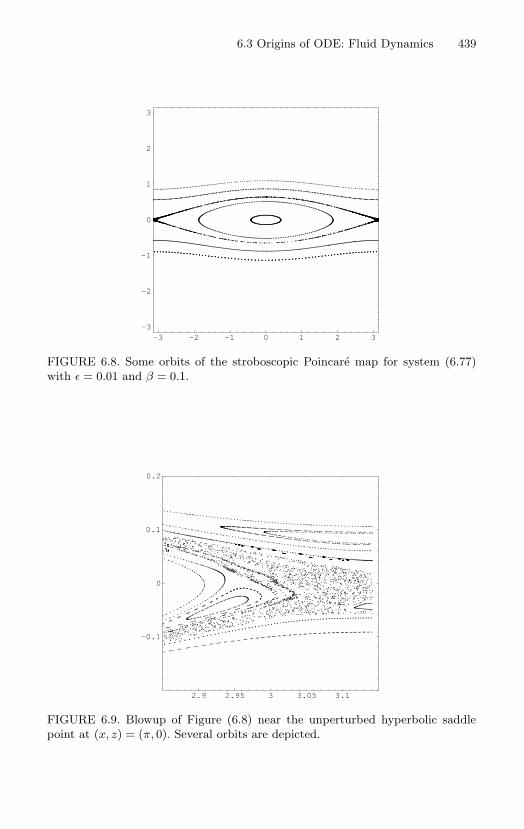
6.3 Origins of ODE: Fluid Dynamics 439
-3 -2 -1 0 1 2 3-3
-2
-1
0
1
2
3
FIGURE 6.8. Some orbits of the stroboscopic Poincare map for system (6.77)with ε = 0.01 and β = 0.1.
2.9 2.95 3 3.05 3.1
-0.1
0
0.1
0.2
FIGURE 6.9. Blowup of Figure (6.8) near the unperturbed hyperbolic saddlepoint at (x, z) = (π, 0). Several orbits are depicted.
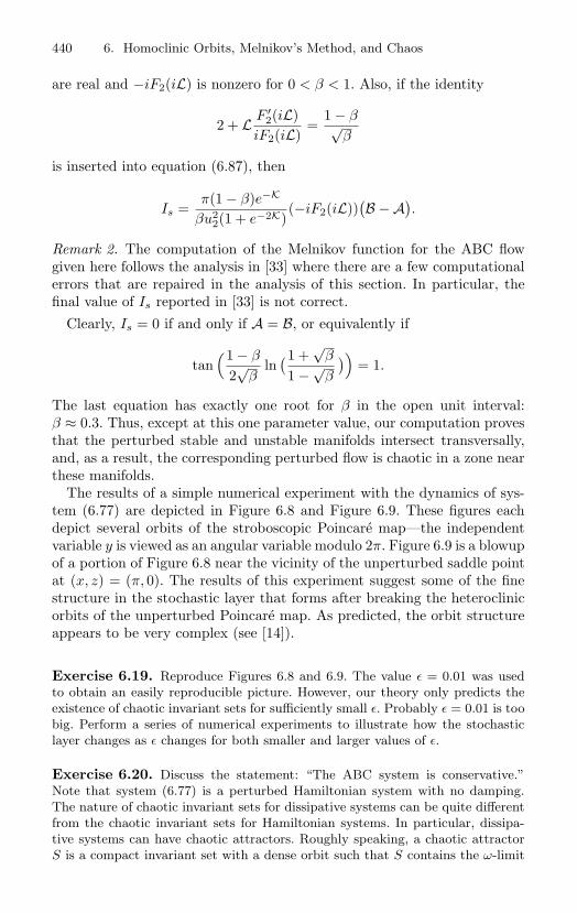
440 6. Homoclinic Orbits, Melnikov’s Method, and Chaos
are real and −iF2(iL) is nonzero for 0 < β < 1. Also, if the identity
2 + L F ′2(iL)
iF2(iL)=
1 − β√β
is inserted into equation (6.87), then
Is =π(1 − β)e−K
βu22(1 + e−2K)
(−iF2(iL))(B − A
).
Remark 2. The computation of the Melnikov function for the ABC flowgiven here follows the analysis in [33] where there are a few computationalerrors that are repaired in the analysis of this section. In particular, thefinal value of Is reported in [33] is not correct.
Clearly, Is = 0 if and only if A = B, or equivalently if
tan(1 − β
2√
βln
(1 +√
β
1 −√
β
))= 1.
The last equation has exactly one root for β in the open unit interval:β ≈ 0.3. Thus, except at this one parameter value, our computation provesthat the perturbed stable and unstable manifolds intersect transversally,and, as a result, the corresponding perturbed flow is chaotic in a zone nearthese manifolds.
The results of a simple numerical experiment with the dynamics of sys-tem (6.77) are depicted in Figure 6.8 and Figure 6.9. These figures eachdepict several orbits of the stroboscopic Poincare map—the independentvariable y is viewed as an angular variable modulo 2π. Figure 6.9 is a blowupof a portion of Figure 6.8 near the vicinity of the unperturbed saddle pointat (x, z) = (π, 0). The results of this experiment suggest some of the finestructure in the stochastic layer that forms after breaking the heteroclinicorbits of the unperturbed Poincare map. As predicted, the orbit structureappears to be very complex (see [14]).
Exercise 6.19. Reproduce Figures 6.8 and 6.9. The value ε = 0.01 was usedto obtain an easily reproducible picture. However, our theory only predicts theexistence of chaotic invariant sets for sufficiently small ε. Probably ε = 0.01 is toobig. Perform a series of numerical experiments to illustrate how the stochasticlayer changes as ε changes for both smaller and larger values of ε.
Exercise 6.20. Discuss the statement: “The ABC system is conservative.”Note that system (6.77) is a perturbed Hamiltonian system with no damping.The nature of chaotic invariant sets for dissipative systems can be quite differentfrom the chaotic invariant sets for Hamiltonian systems. In particular, dissipa-tive systems can have chaotic attractors. Roughly speaking, a chaotic attractorS is a compact invariant set with a dense orbit such that S contains the ω-limit
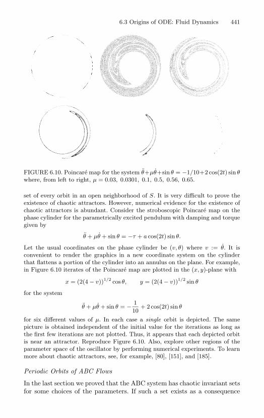
6.3 Origins of ODE: Fluid Dynamics 441
FIGURE 6.10. Poincare map for the system θ+µθ+sin θ = −1/10+2 cos(2t) sin θwhere, from left to right, µ = 0.03, 0.0301, 0.1, 0.5, 0.56, 0.65.
set of every orbit in an open neighborhood of S. It is very difficult to prove theexistence of chaotic attractors. However, numerical evidence for the existence ofchaotic attractors is abundant. Consider the stroboscopic Poincare map on thephase cylinder for the parametrically excited pendulum with damping and torquegiven by
θ + µθ + sin θ = −τ + a cos(2t) sin θ.
Let the usual coordinates on the phase cylinder be (v, θ) where v := θ. It isconvenient to render the graphics in a new coordinate system on the cylinderthat flattens a portion of the cylinder into an annulus on the plane. For example,in Figure 6.10 iterates of the Poincare map are plotted in the (x, y)-plane with
x = (2(4 − v))1/2 cos θ, y = (2(4 − v))1/2 sin θ
for the system
θ + µθ + sin θ = − 110
+ 2 cos(2t) sin θ
for six different values of µ. In each case a single orbit is depicted. The samepicture is obtained independent of the initial value for the iterations as long asthe first few iterations are not plotted. Thus, it appears that each depicted orbitis near an attractor. Reproduce Figure 6.10. Also, explore other regions of theparameter space of the oscillator by performing numerical experiments. To learnmore about chaotic attractors, see, for example, [80], [151], and [185].
Periodic Orbits of ABC Flows
In the last section we proved that the ABC system has chaotic invariant setsfor some choices of the parameters. If such a set exists as a consequence
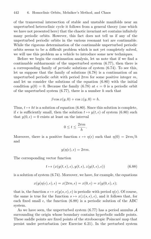
442 6. Homoclinic Orbits, Melnikov’s Method, and Chaos
of the transversal intersection of stable and unstable manifolds near anunperturbed heteroclinic cycle it follows from a general theory (one whichwe have not presented here) that the chaotic invariant set contains infinitelymany periodic orbits. However, this fact does not tell us if any of theunperturbed periodic orbits in the various resonant tori are continuable.While the rigorous determination of the continuable unperturbed periodicorbits seems to be a difficult problem which is not yet completely solved,we will use this problem as a vehicle to introduce some new techniques.
Before we begin the continuation analysis, let us note that if we find acontinuable subharmonic of the unperturbed system (6.77), then there isa corresponding family of periodic solutions of system (6.74). To see this,let us suppose that the family of solutions (6.78) is a continuation of anunperturbed periodic orbit with period 2πm for some positive integer m,and let us consider the solutions of the equation (6.80) with the initialcondition y(0) = 0. Because the family (6.78) at ε = 0 is a periodic orbitof the unperturbed system (6.77), there is a number h such that
β cos x(y, 0) + cos z(y, 0) = h.
Thus, t → ht is a solution of equation (6.80). Since this solution is complete,if ε is sufficiently small, then the solution t → y(t, ε) of system (6.80) suchthat y(0, ε) = 0 exists at least on the interval
0 ≤ t ≤ 2πm
h.
Moreover, there is a positive function ε → η(ε) such that η(0) = 2πm/hand
y(η(ε), ε) = 2πm.
The corresponding vector function
t → (x(y(t, ε), ε), y(t, ε), z(y(t, ε), ε)) (6.88)
is a solution of system (6.74). Moreover, we have, for example, the equations
x(y(η(ε), ε), ε) = x(2πn, ε) = x(0, ε) = x(y(0, ε), ε);
that is, the function s → x(y(s, ε), ε) is periodic with period η(ε). Of course,the same is true for the function s → x(z(s, ε), ε), and it follows that, foreach fixed small ε, the function (6.88) is a periodic solution of the ABCsystem.
As we have seen, the unperturbed system (6.77) has a period annulus Asurrounding the origin whose boundary contains hyperbolic saddle points.These saddle points are fixed points of the stroboscopic Poincare map thatpersist under perturbation (see Exercise 6.21). In the perturbed system
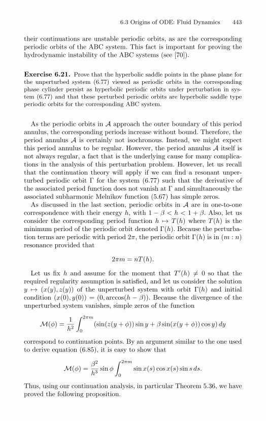
6.3 Origins of ODE: Fluid Dynamics 443
their continuations are unstable periodic orbits, as are the correspondingperiodic orbits of the ABC system. This fact is important for proving thehydrodynamic instability of the ABC systems (see [70]).
Exercise 6.21. Prove that the hyperbolic saddle points in the phase plane forthe unperturbed system (6.77) viewed as periodic orbits in the correspondingphase cylinder persist as hyperbolic periodic orbits under perturbation in sys-tem (6.77) and that these perturbed periodic orbits are hyperbolic saddle typeperiodic orbits for the corresponding ABC system.
As the periodic orbits in A approach the outer boundary of this periodannulus, the corresponding periods increase without bound. Therefore, theperiod annulus A is certainly not isochronous. Instead, we might expectthis period annulus to be regular. However, the period annulus A itself isnot always regular, a fact that is the underlying cause for many complica-tions in the analysis of this perturbation problem. However, let us recallthat the continuation theory will apply if we can find a resonant unper-turbed periodic orbit Γ for the system (6.77) such that the derivative ofthe associated period function does not vanish at Γ and simultaneously theassociated subharmonic Melnikov function (5.67) has simple zeros.
As discussed in the last section, periodic orbits in A are in one-to-onecorrespondence with their energy h, with 1 − β < h < 1 + β. Also, let usconsider the corresponding period function h → T (h) where T (h) is theminimum period of the periodic orbit denoted Γ(h). Because the perturba-tion terms are periodic with period 2π, the periodic orbit Γ(h) is in (m : n)resonance provided that
2πm = nT (h).
Let us fix h and assume for the moment that T ′(h) = 0 so that therequired regularity assumption is satisfied, and let us consider the solutiony → (x(y), z(y)) of the unperturbed system with orbit Γ(h) and initialcondition (x(0), y(0)) = (0, arccos(h − β)). Because the divergence of theunperturbed system vanishes, simple zeros of the function
M(φ) =1h2
∫ 2πm
0(sin(z(y + φ)) sin y + β sin(x(y + φ)) cos y) dy
correspond to continuation points. By an argument similar to the one usedto derive equation (6.85), it is easy to show that
M(φ) =β2
h3 sin φ
∫ 2πm
0sin x(s) cos x(s) sin s ds.
Thus, using our continuation analysis, in particular Theorem 5.36, we haveproved the following proposition.
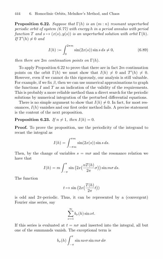
444 6. Homoclinic Orbits, Melnikov’s Method, and Chaos
Proposition 6.22. Suppose that Γ(h) is an (m : n) resonant unperturbedperiodic orbit of system (6.77) with energy h in a period annulus with periodfunction T and s → (x(s), y(s)) is an unperturbed solution with orbit Γ(h).If T ′(h) = 0 and
I(h) :=∫ 2πm
0sin(2x(s)) sin s ds = 0, (6.89)
then there are 2m continuation points on Γ(h).
To apply Proposition 6.22 to prove that there are in fact 2m continuationpoints on the orbit Γ(h) we must show that I(h) = 0 and T ′(h) = 0.However, even if we cannot do this rigorously, our analysis is still valuable.For example, if we fix β, then we can use numerical approximations to graphthe functions I and T as an indication of the validity of the requirements.This is probably a more reliable method than a direct search for the periodicsolutions by numerical integration of the perturbed differential equations.
There is no simple argument to show that I(h) = 0. In fact, for most res-onances, I(h) vanishes and our first order method fails. A precise statementis the content of the next proposition.
Proposition 6.23. If n = 1, then I(h) = 0.
Proof. To prove the proposition, use the periodicity of the integrand torecast the integral as
I(h) =∫ πm
−πm
sin(2x(s)) sin s ds.
Then, by the change of variables s = mσ and the resonance relation wehave that
I(h) = m
∫ π
−π
sin(2x
(nT (h)2π
σ))
sin mσ ds.
The function
t → sin(2x
(T (h)2π
t))
is odd and 2π-periodic. Thus, it can be represented by a (convergent)Fourier sine series, say
∞∑ν=1
bν(h) sin νt.
If this series is evaluated at t = nσ and inserted into the integral, all butone of the summands vanish. The exceptional term is
bν(h)∫ π
−π
sin nνσ sin mσ dσ
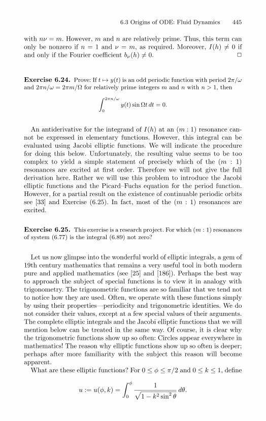
6.3 Origins of ODE: Fluid Dynamics 445
with nν = m. However, m and n are relatively prime. Thus, this term canonly be nonzero if n = 1 and ν = m, as required. Moreover, I(h) = 0 ifand only if the Fourier coefficient bν(h) = 0.
Exercise 6.24. Prove: If t → y(t) is an odd periodic function with period 2π/ωand 2πn/ω = 2πm/Ω for relatively prime integers m and n with n > 1, then
∫ 2πn/ω
0y(t) sin Ωt dt = 0.
An antiderivative for the integrand of I(h) at an (m : 1) resonance can-not be expressed in elementary functions. However, this integral can beevaluated using Jacobi elliptic functions. We will indicate the procedurefor doing this below. Unfortunately, the resulting value seems to be toocomplex to yield a simple statement of precisely which of the (m : 1)resonances are excited at first order. Therefore we will not give the fullderivation here. Rather we will use this problem to introduce the Jacobielliptic functions and the Picard–Fuchs equation for the period function.However, for a partial result on the existence of continuable periodic orbitssee [33] and Exercise (6.25). In fact, most of the (m : 1) resonances areexcited.
Exercise 6.25. This exercise is a research project. For which (m : 1) resonancesof system (6.77) is the integral (6.89) not zero?
Let us now glimpse into the wonderful world of elliptic integrals, a gem of19th century mathematics that remains a very useful tool in both modernpure and applied mathematics (see [25] and [186]). Perhaps the best wayto approach the subject of special functions is to view it in analogy withtrigonometry. The trigonometric functions are so familiar that we tend notto notice how they are used. Often, we operate with these functions simplyby using their properties—periodicity and trigonometric identities. We donot consider their values, except at a few special values of their arguments.The complete elliptic integrals and the Jacobi elliptic functions that we willmention below can be treated in the same way. Of course, it is clear whythe trigonometric functions show up so often: Circles appear everywhere inmathematics! The reason why elliptic functions show up so often is deeper;perhaps after more familiarity with the subject this reason will becomeapparent.
What are these elliptic functions? For 0 ≤ φ ≤ π/2 and 0 ≤ k ≤ 1, define
u := u(φ, k) =∫ φ
0
1√1 − k2 sin2 θ
dθ.
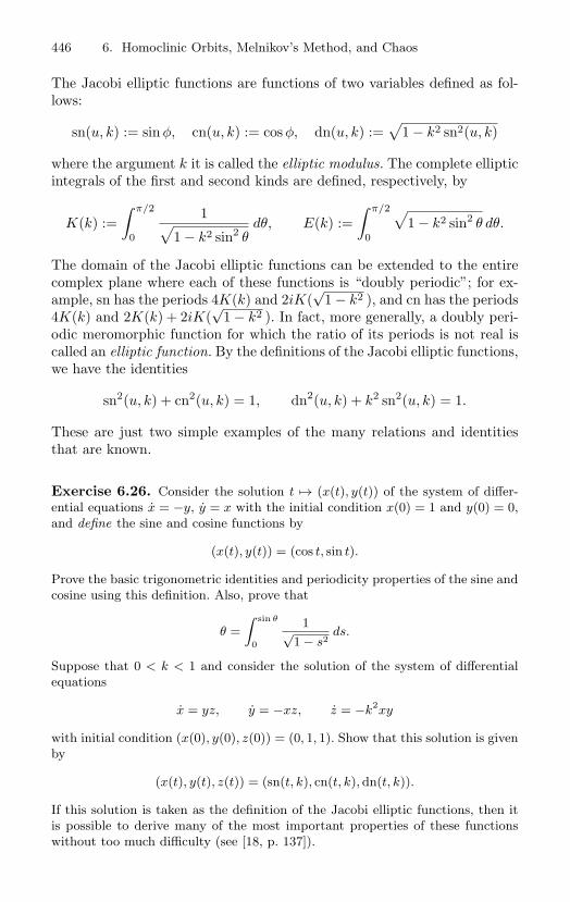
446 6. Homoclinic Orbits, Melnikov’s Method, and Chaos
The Jacobi elliptic functions are functions of two variables defined as fol-lows:
sn(u, k) := sin φ, cn(u, k) := cos φ, dn(u, k) :=√
1 − k2 sn2(u, k)
where the argument k it is called the elliptic modulus. The complete ellipticintegrals of the first and second kinds are defined, respectively, by
K(k) :=∫ π/2
0
1√1 − k2 sin2 θ
dθ, E(k) :=∫ π/2
0
√1 − k2 sin2 θ dθ.
The domain of the Jacobi elliptic functions can be extended to the entirecomplex plane where each of these functions is “doubly periodic”; for ex-ample, sn has the periods 4K(k) and 2iK(
√1 − k2 ), and cn has the periods
4K(k) and 2K(k) + 2iK(√
1 − k2 ). In fact, more generally, a doubly peri-odic meromorphic function for which the ratio of its periods is not real iscalled an elliptic function. By the definitions of the Jacobi elliptic functions,we have the identities
sn2(u, k) + cn2(u, k) = 1, dn2(u, k) + k2 sn2(u, k) = 1.
These are just two simple examples of the many relations and identitiesthat are known.
Exercise 6.26. Consider the solution t → (x(t), y(t)) of the system of differ-ential equations x = −y, y = x with the initial condition x(0) = 1 and y(0) = 0,and define the sine and cosine functions by
(x(t), y(t)) = (cos t, sin t).
Prove the basic trigonometric identities and periodicity properties of the sine andcosine using this definition. Also, prove that
θ =∫ sin θ
0
1√1 − s2
ds.
Suppose that 0 < k < 1 and consider the solution of the system of differentialequations
x = yz, y = −xz, z = −k2xy
with initial condition (x(0), y(0), z(0)) = (0, 1, 1). Show that this solution is givenby
(x(t), y(t), z(t)) = (sn(t, k), cn(t, k), dn(t, k)).
If this solution is taken as the definition of the Jacobi elliptic functions, then itis possible to derive many of the most important properties of these functionswithout too much difficulty (see [18, p. 137]).
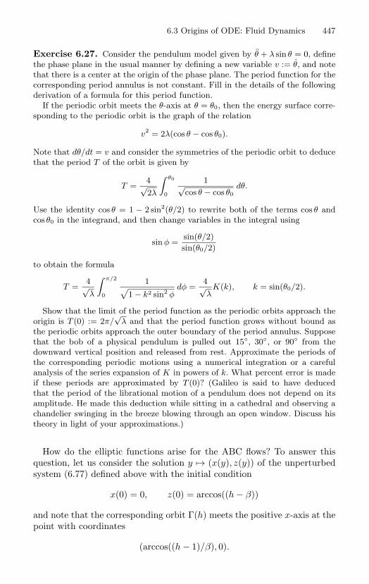
6.3 Origins of ODE: Fluid Dynamics 447
Exercise 6.27. Consider the pendulum model given by θ + λ sin θ = 0, definethe phase plane in the usual manner by defining a new variable v := θ, and notethat there is a center at the origin of the phase plane. The period function for thecorresponding period annulus is not constant. Fill in the details of the followingderivation of a formula for this period function.
If the periodic orbit meets the θ-axis at θ = θ0, then the energy surface corre-sponding to the periodic orbit is the graph of the relation
v2 = 2λ(cos θ − cos θ0).
Note that dθ/dt = v and consider the symmetries of the periodic orbit to deducethat the period T of the orbit is given by
T =4√2λ
∫ θ0
0
1√cos θ − cos θ0
dθ.
Use the identity cos θ = 1 − 2 sin2(θ/2) to rewrite both of the terms cos θ andcos θ0 in the integrand, and then change variables in the integral using
sin φ =sin(θ/2)sin(θ0/2)
to obtain the formula
T =4√λ
∫ π/2
0
1√1 − k2 sin2 φ
dφ =4√λ
K(k), k = sin(θ0/2).
Show that the limit of the period function as the periodic orbits approach theorigin is T (0) := 2π/
√λ and that the period function grows without bound as
the periodic orbits approach the outer boundary of the period annulus. Supposethat the bob of a physical pendulum is pulled out 15, 30, or 90 from thedownward vertical position and released from rest. Approximate the periods ofthe corresponding periodic motions using a numerical integration or a carefulanalysis of the series expansion of K in powers of k. What percent error is madeif these periods are approximated by T (0)? (Galileo is said to have deducedthat the period of the librational motion of a pendulum does not depend on itsamplitude. He made this deduction while sitting in a cathedral and observing achandelier swinging in the breeze blowing through an open window. Discuss histheory in light of your approximations.)
How do the elliptic functions arise for the ABC flows? To answer thisquestion, let us consider the solution y → (x(y), z(y)) of the unperturbedsystem (6.77) defined above with the initial condition
x(0) = 0, z(0) = arccos((h − β))
and note that the corresponding orbit Γ(h) meets the positive x-axis at thepoint with coordinates
(arccos((h − 1)/β), 0).
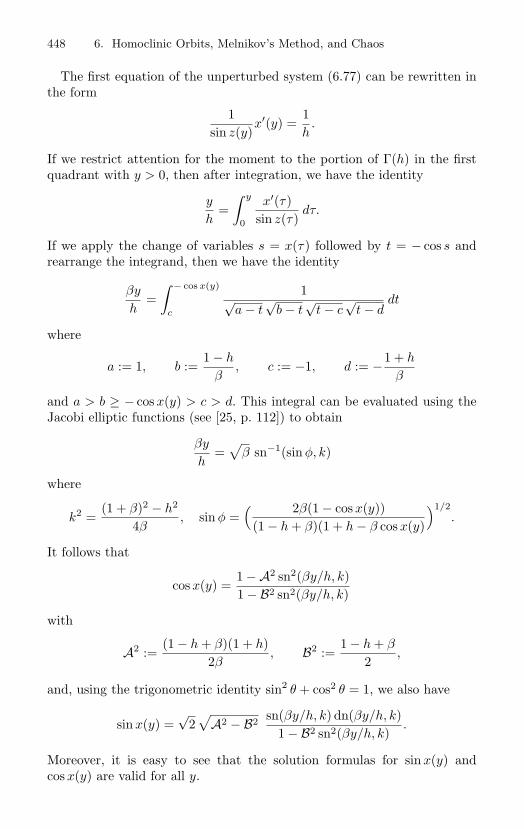
448 6. Homoclinic Orbits, Melnikov’s Method, and Chaos
The first equation of the unperturbed system (6.77) can be rewritten inthe form
1sin z(y)
x′(y) =1h
.
If we restrict attention for the moment to the portion of Γ(h) in the firstquadrant with y > 0, then after integration, we have the identity
y
h=
∫ y
0
x′(τ)sin z(τ)
dτ.
If we apply the change of variables s = x(τ) followed by t = − cos s andrearrange the integrand, then we have the identity
βy
h=
∫ − cos x(y)
c
1√a − t
√b − t
√t − c
√t − d
dt
where
a := 1, b :=1 − h
β, c := −1, d := −1 + h
β
and a > b ≥ − cos x(y) > c > d. This integral can be evaluated using theJacobi elliptic functions (see [25, p. 112]) to obtain
βy
h=
√β sn−1(sin φ, k)
where
k2 =(1 + β)2 − h2
4β, sin φ =
( 2β(1 − cos x(y))(1 − h + β)(1 + h − β cos x(y)
)1/2.
It follows that
cos x(y) =1 − A2 sn2(βy/h, k)1 − B2 sn2(βy/h, k)
with
A2 :=(1 − h + β)(1 + h)
2β, B2 :=
1 − h + β
2,
and, using the trigonometric identity sin2 θ + cos2 θ = 1, we also have
sin x(y) =√
2√
A2 − B2 sn(βy/h, k) dn(βy/h, k)1 − B2 sn2(βy/h, k)
.
Moreover, it is easy to see that the solution formulas for sin x(y) andcos x(y) are valid for all y.
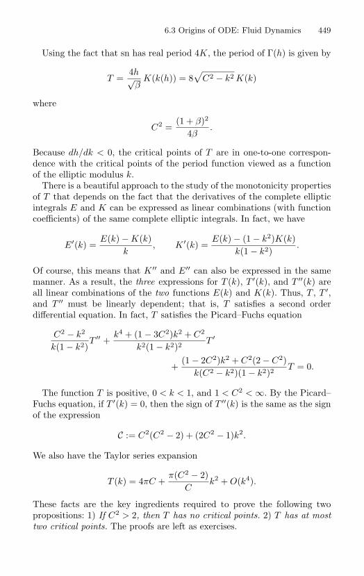
6.3 Origins of ODE: Fluid Dynamics 449
Using the fact that sn has real period 4K, the period of Γ(h) is given by
T =4h√β
K(k(h)) = 8√
C2 − k2 K(k)
where
C2 =(1 + β)2
4β.
Because dh/dk < 0, the critical points of T are in one-to-one correspon-dence with the critical points of the period function viewed as a functionof the elliptic modulus k.
There is a beautiful approach to the study of the monotonicity propertiesof T that depends on the fact that the derivatives of the complete ellipticintegrals E and K can be expressed as linear combinations (with functioncoefficients) of the same complete elliptic integrals. In fact, we have
E′(k) =E(k) − K(k)
k, K ′(k) =
E(k) − (1 − k2)K(k)k(1 − k2)
.
Of course, this means that K ′′ and E′′ can also be expressed in the samemanner. As a result, the three expressions for T (k), T ′(k), and T ′′(k) areall linear combinations of the two functions E(k) and K(k). Thus, T , T ′,and T ′′ must be linearly dependent; that is, T satisfies a second orderdifferential equation. In fact, T satisfies the Picard–Fuchs equation
C2 − k2
k(1 − k2)T ′′ +
k4 + (1 − 3C2)k2 + C2
k2(1 − k2)2T ′
+(1 − 2C2)k2 + C2(2 − C2)
k(C2 − k2)(1 − k2)2T = 0.
The function T is positive, 0 < k < 1, and 1 < C2 < ∞. By the Picard–Fuchs equation, if T ′(k) = 0, then the sign of T ′′(k) is the same as the signof the expression
C := C2(C2 − 2) + (2C2 − 1)k2.
We also have the Taylor series expansion
T (k) = 4πC +π(C2 − 2)
Ck2 + O(k4).
These facts are the key ingredients required to prove the following twopropositions: 1) If C2 > 2, then T has no critical points. 2) T has at mosttwo critical points. The proofs are left as exercises.
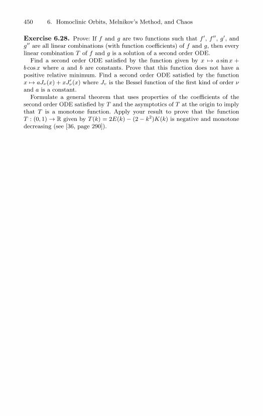
450 6. Homoclinic Orbits, Melnikov’s Method, and Chaos
Exercise 6.28. Prove: If f and g are two functions such that f ′, f ′′, g′, andg′′ are all linear combinations (with function coefficients) of f and g, then everylinear combination T of f and g is a solution of a second order ODE.
Find a second order ODE satisfied by the function given by x → a sin x +b cos x where a and b are constants. Prove that this function does not have apositive relative minimum. Find a second order ODE satisfied by the functionx → aJν(x) + xJ ′
ν(x) where Jv is the Bessel function of the first kind of order νand a is a constant.
Formulate a general theorem that uses properties of the coefficients of thesecond order ODE satisfied by T and the asymptotics of T at the origin to implythat T is a monotone function. Apply your result to prove that the functionT : (0, 1) → R given by T (k) = 2E(k) − (2 − k2)K(k) is negative and monotonedecreasing (see [36, page 290]).
7Averaging
This chapter is an introduction to the method of averaging—a far-reachingand rich mathematical subject that has many important applications. Ourapproach to the subject is through perturbation theory; for example, we willdiscuss the existence of periodic orbits for periodically forced oscillators.However, we will also introduce some additional ideas from the theory ofaveraging that have far-reaching implications beyond the scope of this book.
Recall that we have already discussed informally in Section 3.2 appli-cations of the method of averaging to various perturbations of a Keple-rian binary. While an understanding of these applications is not requiredas background for the mathematical theory in this chapter, a review ofthe Keplerian perturbation problem in celestial mechanics is highly recom-mended as a wonderful way to gain an appreciation for the subject at hand.For further study there are many excellent mathematical treatments of thetheory and applications of the method of averaging (see, for example, [10],[12], [83], [110], [130], [157] and [80], [101], [113], [133], [185].)
7.1 The Averaging Principle
Let us consider a family of differential equations given by
u = f(u) + εg(u, t, ε), u ∈ RM (7.1)
452 7. Averaging
where the perturbation term is periodic in time with period η > 0. Also,let us suppose that the unperturbed system
u = f(u), u ∈ RM (7.2)
is “integrable.” The precise definition of an integrable system will not beneeded; rather, we will assume that a region of the phase space for theunperturbed system is foliated by invariant tori. In the planar case, this isexactly the assumption that the unperturbed system has a period annulus.
Special coordinates, called action-angle variables, can always be definedon the region of the phase space foliated by invariant tori so that theunperturbed system, when expressed in the new coordinates, has a usefulstandard form (see Section 7.3). In this section we will construct the action-angle variables for the harmonic oscillator; the Delaunay elements definedfor the Kepler problem in Section 3.2 provide a more substantial example.
Recall that the Hamiltonian H : R × R → R for the harmonic oscillator,the total energy of the mechanical system, is given by
H(q, p) :=12p2 +
12ω2q2,
and the entire punctured plane is a period annulus for the correspondingHamiltonian system
q = p, p = −ω2q. (7.3)
Moreover, the periodic orbits of this system correspond to level sets of H.In particular, each level set is an ellipse. Similarly, if a general one-degree-of-freedom Hamiltonian system
q =∂H
∂p, p = −∂H
∂q(7.4)
with Hamiltonian H : R×R → R has a period annulus A, then the periodicorbits in A are regular level sets of H.
In case A is a period annulus for the Hamiltonian system (7.4), letM(q0, p0) denote the periodic orbit that passes through the point (q0, p0) ∈A, and note that M(q0, p0) is a subset of the regular energy surface
(q, p) ∈ R2 : H(q, p) = H(q0, p0).
The function I : A → R defined by
I(q, p) :=12π
∫M(q,p)
p dq (7.5)
is called the action of the Hamiltonian system on the period annulus. Itsvalue at (q, p) is the normalized area of the region in the phase spaceenclosed by the periodic orbit M(q, p).
7.1 The Averaging Principle 453
For the harmonic oscillator, the action at (q0, p0) = (0, 0) is 1/(2π) mul-tiplied by the area enclosed by the ellipse M(q0, p0) with equation
12p2 +
12ω2q2 =
12a2
where a := (p20 + ω2q2
0)1/2. The intercept of this ellipse with the p-axisis (q, p) = (0, a) and its intercept with the q-axis is (a/ω, 0). Using thefact that the area of an ellipse is π times the product of the lengths ofits semimajor and semiminor axes, let us observe that the action for theharmonic oscillator is proportional to its Hamiltonian; in fact,
I(q, p) =a2
2ω=
1ω
H(q, p).
Since the Hamiltonian is constant on orbits, the action is a first integral,that is, I = 0.
To define the angular variable, let Σ be a Poincare section in the periodannulus A, and let T denote the associated period function. Also, for eachpoint (q, p) ∈ A that lies on an orbit that crosses Σ, define the time mapτ that assigns to the point (q, p) the minimum positive time required toreach (q, p) along the solution of the system that starts at the intersectionpoint σ(q, p) of the orbit M(q, p) and the section Σ. With this notation,the angular variable θ is defined by
θ(q, p) :=2π
T (σ(q, p))τ(q, p). (7.6)
For the harmonic oscillator, every periodic orbit has the same period2π/ω. Moreover, the flow is given by a uniform linear rotation. Thus, forthe time map τ , we have that τ = 1. Hence, the angular variable satisfiesthe differential equation θ = ω. In the general case, the frequency of theperiodic orbit may be a nonconstant function of the action, and in thiscase, the differential equation for the angular variable is θ = ω(I).
The fact that the function (q, p) → (I(q, p), θ(q, p)) defines a polar coor-dinate chart on an annular subset of A is proved in Section 7.3 below. Thus,the change to action-angle variables is nonsingular, and the Hamiltoniansystem in action-angle variables, that is, the system
I = 0, θ = ω(I),
can be viewed as a system of differential equations on the phase cylinder:the product of a line with coordinate I and a one-dimensional torus withcoordinate θ (see Section 1.7.4).
More generally, a multidimensional integrable system has an invariantmanifold that is topologically the cross product of a Cartesian space R
M
454 7. Averaging
and a torus TN . In this case, action-angle variables I and θ can be defined
in RM × T
N such that the integrable system is given by
I = 0, θ = ω(I) (7.7)
where I ∈ RM and θ ∈ T
N are vector variables. This is the standardform for an integrable system, the starting point for classical perturbationtheory.
The method of averaging is a powerful tool that is used to obtain andanalyze approximate solutions for perturbations of integrable systems, thatis, for systems of differential equations of the form
I = εF (I, θ), θ = ω(I) + εG(I, θ) (7.8)
where θ is a vector of angular variables defined modulo 2π, both F and Gare 2π-periodic functions of their second argument, and ε > 0 is considereda small parameter. Poincare called the analysis of systems of the form (7.8)“the fundamental problem of dynamical systems.”
In a physical application, the mathematical model is usually not deriveddirectly in action-angle variables. Thus, even if the unperturbed modelsystem is integrable, and even if we can construct action-angle variables ina region of its phase space, then in order to obtain a perturbation problemin the standard form (7.8) we still have the formidable task of transformingthe perturbed vector field to the new coordinates given by the action-anglevariables for the unperturbed system. However, the benefits of workingwith the standard form system (7.8) often justify the effort required toperform the coordinate transformation. This fact is clearly illustrated bythe analysis of the perturbed Kepler problem in Section 3.2.
The dynamics of the unperturbed system (7.7) are very simple. In fact,the solution with the initial condition (I, θ) = (I0, θ0) is given by I(t) ≡ I0and θ(t) = ω(I0)t + ω0. In effect, the actions specify a particular torus inthe phase space, and the angles vary linearly on this torus.
Definition 7.1. Suppose that I0 is in RM . The N -dimensional invariant
torus
(I, θ) ∈ RM × R
N : I = I0
for the system (7.7) is resonant if there is an integer vector K of length Nsuch that 〈K, ω(I0)〉 = 0 where 〈 〉 denotes the usual inner product. In thiscase we also say that the frequencies, the components of the vector ω(I0),are in resonance.
If an invariant torus for the system (7.7) is not resonant, then every orbiton the torus is dense. In case N = 2, every orbit on a resonant torus isperiodic. Matters are not quite so simple for N > 2 where the existenceof a resonance relation does not necessarily mean that all orbits on the
7.1 The Averaging Principle 455
corresponding invariant torus are periodic. This is just one indication ofthe fact that the dynamics of systems with more than two frequencies is ingeneral quite different from the dynamics of systems with one frequency.However, in all cases, the existence of resonant tori plays a central role inthe analysis of the perturbed dynamical system.
In Chapter 5 some aspects of the near resonant behavior of the planarcase of system (7.1) are discussed in detail, especially, the continuationtheory for resonant unperturbed periodic solutions. As we have seen, thisspecial case, and the general multidimensional time-periodic system (7.1)can be viewed as systems on a phase cylinder by the introduction of a newangular variable so that the extended system is given by
u = f(u) + εg(u, τ, ε), τ = 1. (7.9)
Let us note the obvious fact that if the system u = f(u) is integrable, thenso is system (7.9) at ε = 0.
If u ∈ R2 and the system u = f(u) has a period annulus A, then it is
integrable. In this case, a subset of the three-dimensional phase space forthe extended system (7.9) at ε = 0 is filled with invariant two-dimensionaltori corresponding to the periodic orbits in A. Thus, there is one actionvariable, which has a constant value on each periodic orbit, and two anglevariables. One of the angular variables is τ ; the other is the angle variabledefined for the action-angle variables of the unperturbed planar system.
The basic idea that leads to the development of the method of averagingarises from an inspection of the system (7.8). The time derivatives of theactions are all proportional to ε. Hence, if ε is small, the actions would beexpected to remain near their constant unperturbed values over a long timescale. On the other hand, the angles are oscillating rapidly relative to theslow change of the actions. Thus, the slow evolution of the actions awayfrom their initial values is revealed by averaging over the high frequencyoscillations due to the relatively fast changes of the angles.
In most applications, we are indeed interested in the evolution of theactions, not the angles. For example, in the Kepler problem, the distance ofa planet from a star is given by an action variable whereas its exact positionin the sky also requires the specification of an angle. As we observe a planetand make predictions about its future, we are probably more interested inthe evolution of the distance between the planet and the star than the exactposition of the planet relative to the star.
Averaging Principle. If I = I0 is the initial value for the action variablesin system (7.8), then, for sufficiently small ε, a useful approximation of theevolution of the actions of this system is given by the solution of the initialvalue problem
J = εF (J), J(0) = I0, (7.10)
456 7. Averaging
called the averaged system, where F is the function defined by
F (J) :=1
(2π)N
∫TN
F (J, θ) dθ.
The averaging principle has a long history that is deeply rooted in pertur-bation problems that arise in celestial mechanics (see, for example, [157]).However, it is clear from the use of the phrase “useful approximation” thatthe averaging principle is not a theorem. In a physical application, it mightbe reasonable to use the averaging principle to replace a mathematicalmodel in the form of the differential equation (7.8) by the correspondingaveraged system (7.10), to use the averaged system to make a prediction,and then to test the prediction against the results of a physical experi-ment. However, to ascertain the utility of the approximation obtained byaveraging, a mathematical theory is required.
The next theorem (the averaging theorem) validates the averaging prin-ciple under the hypothesis that there is exactly one angular variable. Thestatement of the theorem is rather complicated. However, attention mustbe paid to the main points: There is a change of variables for system (7.8)such that the first order truncation with respect to ε of the transformeddifferential equation for the actions is exactly the averaged system (7.10);and the solution of this averaged system is O(ε) close to the solutions ofthe original differential equation with the same initial action over a timeinterval whose length is O(1/ε).
Theorem 7.2 (Averaging Theorem). Suppose that system (7.8) is de-fined on U × T where U is an open subset of R
M .
(i) If there is some number λ such that ω(I) > λ > 0 for all I ∈ U ,then there is a bounded open ball B contained in U , a number ε1 > 0,and a smooth function k : B × T → B such that for each I ∈ B thefunction θ → k(I, θ) is 2π-periodic, the function I → I + εk(I, θ) isinvertible on B for 0 ≤ ε < ε1, and the change of coordinates givenby
L = I + εk(I, θ) (7.11)
transforms the system (7.8) to the form
L = εF (L) + ε2F1(L, θ, ε), θ = ω(L) + εG1(L, θ, ε) (7.12)
where
F (L) =12π
∫ π
0F (L, θ) dθ
and both of the functions F1 and G1 are 2π-periodic with respect totheir second arguments.
7.1 The Averaging Principle 457
(ii) If in addition T > 0, B0 is an open ball whose closure is containedin the interior of B, and if for each I0 ∈ B the number τ(I0) denotesthe largest number less than or equal to T such that the solution ofthe averaged system (7.10) with initial condition J(0) = I0 is in theclosure of B0 for 0 ≤ t ≤ τ(I0), then there are positive numbersε2 ≤ ε1 and C such that for each I0 ∈ B0 and for 0 ≤ ε < ε2all solutions t → (I(t), θ(t)) of the system (7.8) with initial valueI(0) = I0 are approximated by the solution t → J(t) of the averagedsystem (7.10) with J(0) = I0 as follows:
|I(t) − J(t)| < Cε
on the time interval given by 0 ≤ εt < τ(I0).
Proof. To prove statement (i), define a new function F on U ×T given by
F (L, θ) := F (L, θ) − F (L),
and let k denote the solution of the differential equation
∂k
∂θ(L, θ) = − 1
ω(L)F (L, θ) (7.13)
with the initial condition k(L, 0) = 0; that is, k is given by
k(L, θ) = − 1ω(L)
∫ θ
0F (L, s) ds.
Note that k is defined on U × T. Moreover, the function θ → k(L, θ) is2π-periodic. Indeed, if we fix L and define a new function
k(θ) = k(L, θ + 2π) − k(L, θ),
then the result follows from the fact that k(0) = 0 and k′(θ) ≡ 0. (Thedefinition of k uses the fact that there is only one angle. It is preciselythe definition of the “averaging transformation” that is problematic whenthere are several angles.)
In order to have L = I + εk(I, θ) define an averaging transformation, wemust show that the transformation is invertible. To this end, consider thesmooth function K : U × U × T × R → R
M given by
(I, L, θ, ε) → I + εk(I, θ) − L.
For each point ξ = (L, θ) in c(B) × T (here, the notation c denotesthe closure of the set), we have that K(L, L, θ, 0) = 0 and the partialderivative KI(L, L, θ, 0) is the identity transformation of R
M . Therefore,by the implicit function theorem, there is a product neighborhood Γξ × γξ
458 7. Averaging
contained in (U × T) × R and containing the point (ξ, 0), and a smoothfunction Hξ : Γξ × γξ → U such that
Hξ(L, θ, ε) + εk(Hξ(L, θ, ε), θ) = L
for all ((L, θ), ε) ∈ Γξ × γξ. In other words the function L → Hξ(L, θ, ε) isa local inverse for the function I → I + εk(I, θ). Moreover, if (I, (L, θ), ε) ∈U × Γξ × γξ is such that K(I, L, θ, ε) = 0, then I = Hξ(L, θ, ε).
Using the fact that c(B)×T is compact, let us note that there is a finitecollection of the neighborhoods Γξ ×γξ that cover B×T. Also, let Γ denotethe union of the corresponding Γξ, and let γ denote the intersection of thecorresponding intervals on the real line. We have that B ⊂ Γ and that thereis some ε0 such that γ contains the closed interval [0, ε0].
The function k has a global Lipschitz constant Lip(k) on the compactset c(B) × T. Let us define ε1 > 0 such that
ε1 < min 1
Lip(k), ε0
.
If θ ∈ T and 0 ≤ ε ≤ ε1, then the map I → I + εk(I, θ) is injective. In fact,if
I1 + εk(I1, θ) = I2 + εk(I2, θ),
then
|I1 − I2| = |ε|Lip(k)|I1 − I2| < |I1 − I2|,
and therefore I1 = I2. It follows that there is a function H : Γ×T×[0, ε1] →B such that H is the “global” inverse; that is,
H(L, θ, ε) + εk(H(L, θ, ε), θ) = L.
By the uniqueness of the smooth local inverses Hξ, the function H mustagree with each function Hξ on the intersection of their domains. Thus, His smooth and we have defined a coordinate transformation L := I+εk(I, θ)on B×T× [0, ε1]. Moreover, by expanding H in a Taylor series at ε = 0 andwith the first order remainder given by H, we see that I = L + εH(I, θ, ε).Moreover, it is easy to check that θ → H(I, θ, ε) is a 2π-periodic function.
Using the coordinate transformation, we have that
L = I + ε∂k
∂II + ε
∂k
∂θθ
= εF (I, θ) + ε∂k
∂I(I, θ)(εF (I, θ)) + ε
∂k
∂θ(I, θ)(ω(I) + εG(I, θ))
= ε(F (I, θ) +∂k
∂θ(I, θ)ω(I)) + ε2α(I, θ)
7.1 The Averaging Principle 459
where
α(I, θ) :=∂k
∂I(I, θ)F (I, θ) +
∂k
∂θ(I, θ)G(I, θ).
Moreover, using the inverse transformation and Taylor’s theorem, there isa function F1 such that
L = ε(F (L, θ) +∂k
∂θ(L, θ)ω(L)) + ε2F1(L, θ, ε). (7.14)
If the formula for the partial derivative of k, equation (7.13), is insertedinto the equation (7.14), the new differential equation is given by
L = ε(F (L, θ) + F (L) − F (L, θ)) + ε2β(L, θ, ε).
Thus, the coordinate transformation (7.11) applied to the system (7.8)yields a new system of the form
L = εF (L) + ε2F1(L, θ, ε),θ = ω(L) + εG1(L, θ, ε). (7.15)
This completes the proof of statement (i).To prove the asymptotic estimate in statement (ii), consider the differ-
ential equation for L−J obtained by subtracting the averaged system fromthe first differential equation of the system (7.15), and then integrate toobtain
L(t) − J(t) = L(0) − J(0) + ε
∫ t
0F (L(s)) − F (J(s)) ds
+ ε2∫ t
0F1(L(s), θ(s), ε) ds.
If Lip(F ) > 0 is a Lipschitz constant for F , and if B is an upper boundfor the function
(L, θ, ε) → |F1(L, θ, ε)|
on the compact space c(B) × T × [0, ε1], then we have the estimate
|L(t) − J(t)| ≤ |L(0) − J(0)| + ε Lip(F )∫ t
0|L(s) − J(s)| ds + ε2Bt
(7.16)
provided that L(t) remains in c(B).An application of the specific Gronwall lemma from Exercise 2.3 to the
inequality (7.16) yields the following estimate
|L(t) − J(t)| ≤(|L(0) − J(0)| + ε
B
Lip(F )
)eε Lip(F )t.
460 7. Averaging
We also have that
L(0) = I(0) + εk(I(0), θ(0)), I(0) = J(0).
Thus, if 0 ≤ εt ≤ τ(I(0)), where τ is defined in the statement of thetheorem, then there is a constant C0 such that
|L(t) − J(t)| ≤ C0ε (7.17)
provided that L(t) remains in c(B).Note that L(t) is in c(B), as long as |L(t)−J(t)| is less than the minimum
distance between the boundaries of B0 and B. If 0 < ε2 < ε1 is chosen sothat C0/ε2 is less than this distance, then the estimate (7.17) ensures thatL(t) is in c(B) on the time interval 0 ≤ εt ≤ τ(I(0)).
Finally, let C1 be an upper bound for the function
(L, θ) → |k(L, θ)|
and note that for t in the range specified above we have the inequality
|I(t) − J(t)| ≤ |I(t) − L(t)| + |L(t) − J(t)| ≤ εC1 + εC0.
Therefore, with C := C0 + C1, we have the required asymptotic estimate.
7.2 Averaging at Resonance
In this section we will demonstrate the remarkable fact that some of theimportant features of the near resonant dynamics of all oscillators are de-termined by the dynamical behavior of an associated one-degree-of-freedomoscillator that resembles a perturbed pendulum with torque. We will alsogive some examples to show that the averaging principle is not always ap-plicable in multifrequency systems.
Let us consider the system (7.1) with u ∈ RM+N where the period of
the perturbation is η = 2π/Ω and where the unperturbed system has aninvariant set that is foliated by N -dimensional invariant tori. In this case, ifaction-angle variables (I, ϕ) ∈ R
M×TN are introduced, then the differential
equation is expressed in the form
I = εF (I, ϕ, t) + O(ε2),ϕ = ω(I) + εG(I, ϕ, t) + O(ε2). (7.18)
Moreover, it is 2π-periodic in each component of the N -dimensional vectorof angles and 2π/Ω-periodic in time. By introducing an additional angular
7.2 Averaging at Resonance 461
variable τ , system (7.18) is equivalent to the autonomous system with Mactions and N + 1 angles given by
I = εF (I, ϕ, τ/Ω) + O(ε2),ϕ = ω(I) + εG(I, ϕ, τ/Ω) + O(ε2),τ = Ω. (7.19)
Suppose that there is a resonance relation given in the form
〈K, ω(I)〉 = nΩ (7.20)
where K is an integer vector of length M , and n is an integer such thatthe components of K and the integer n have no common factors. The set
RK,n := (I, ϕ, τ) : 〈K, ω(I)〉 = nΩ
corresponding to the resonance relation (7.20), which is generally a hyper-surface in the phase space, is called a resonant manifold. Our goal is todescribe the perturbed dynamics of the system (7.19) near this resonantmanifold. To do this, we will use yet another set of new coordinates thatwill be introduced informally and abstractly. In practice, as we will demon-strate later, the appropriate new coordinates are chosen using the ideas ofthe abstract construction; but, their precise definition depends on specialfeatures of the system being studied.
The set
AK,n := I : 〈K, ω(I)〉 = nΩ,
is the intersection of the resonant manifold with the “action space.” This setis generally a manifold in R
M and is also often called a resonant manifold.However, to distinguish AK,n from RK,n, let us call AK,n the resonantlayer associated with the resonance relation (7.20).
A point in the action space is determined by its “distance” from theresonant layer and by its projection to the resonant layer. In particular,there are local coordinates defined in a neighborhood of the resonant layer,or at least near a portion of this manifold, given by
r = 〈K, ω(I)〉 − nΩ, z = A(I)
where r is a measure of the distance of the point with action I to theresonant layer and the (M−1)-dimensional vector z is the vector coordinateof the projection, denoted by the smooth map A, of the point I to theresonant layer AK,n. However, as we will soon see, it is convenient to use thestretched distance ρ = r/
√ε as a new coordinate rather than the distance
measured by r.Let us also define new angular variables
ψ = 〈K, ϕ〉 − nτ, χ = B(ϕ, τ)
462 7. Averaging
where the vector function B : TN+1 → T
N+1 is chosen so that the transfor-mation to the new angles is invertible. Of course, B must also be 2π-periodicin each component of ϕ and in τ .
In the new coordinates ρ, z, ψ, χ, the system (7.19) has the form
ρ =√
ε〈K, Dω(I)F (I, φ, τ/Ω)〉 + O(ε),z = O(ε),ψ =
√ερ + O(ε3/2),
χ = O(1) (7.21)
provided that I, φ, and τ are viewed as functions of the new coordinates.In system (7.21), ρ and ψ are slow variables, the M − 1 variables repre-
sented by the vector z are “super slow,” and χ is an N -dimensional vectorof fast variables. In keeping with the averaging principle, we will averageover the fast (angular) variables, although we have provided no theoret-ical justification for doing so unless N = 1. At any rate, the differentialequations obtained by averaging over the fast variables in system (7.21) iscalled the partially averaged system at the resonance.
To leading order in µ :=√
ε, the partially averaged system at the reso-nance is
ρ = µ〈K, Dω(I)F ∗(I, ψ)〉,z = 0,
ψ = µρ (7.22)
where F ∗ is obtained by averaging the function
χ → F (I, φ(ψ, χ), τ(ψ, χ)/Ω).
Here we have used the names of the original variables for the correspondingaveraged variables even though this is a dangerous practice!
The function F ∗ is periodic in its second argument with period someintegral multiple of 2π. In particular, using Fourier series, there is a constantvector c(I) and a vector-valued periodic function ψ → h(I, ψ) with zeroaverage such that
F ∗(I, ψ) = c(I) + h(I, ψ).
Also, we can easily obtain the expansion, in powers of µ, of the functionDω expressed in the new coordinates. In fact, because
I(r, z) = I(µρ, z) = I(0, z) + O(µ),
it follows that Dω(I) = Dω(I(0, z)) + O(µ).Under the generic assumption that
〈K, Dω(I(0, z))F ∗(I(0, z), ψ)〉 = 0,
7.2 Averaging at Resonance 463
that is, the vector field corresponding to the averaged system is trans-verse to the resonant manifold, if we take into account system (7.22) andthe above definitions, then there are real-valued functions z → p(z) and(z, ψ) → q(z, ψ) such that our first order approximation to the partiallyaveraged system has the form
ρ = µ(p(z) + q(z, ψ)),z = 0ψ = µρ. (7.23)
Finally, if we define a slow time variable s = µt and take into accountthe fact that z is a constant of the motion, then we may as well view thesystem (7.23) as the following parametrized family of differential equationswith parameter z:
dρ
ds= p(z) + q(z, ψ),
dψ
ds= ρ, (7.24)
or equivalently
d2ψ
ds2 − q(z, ψ) = p(z) (7.25)
where the function ψ → q(z, ψ) is periodic with average zero.In accordance with the usual physical interpretation of the differential
equation (7.25), we have just obtained a wonderful result: Near a reso-nance, every oscillator behaves like a “pendulum” influenced by a constanttorque. Of course, the precise nature of the dynamical behavior near the res-onance depends on the functions p and q in the differential equation (7.25)and on the perturbation terms that appear in the higher order approxima-tions of the partially averaged system. In particular, let us note that thecoefficients of the pendulum equation are functions of the super slow vari-ables. Thus, they vary slowly with the slow time. A rigorous description ofthe motion predicted by the partially averaged system is highly nontrivialand not yet completely understood. However, our result certainly providesa fundamental insight into the near resonant dynamics of oscillators. Also,this result provides a very good reason to study the dynamics of perturbedpendulum models.
Consider the simple pendulum with constant torque (equation (7.25)with p(z) = c and q(z, ψ) := −λ sin ψ) given by
ρ = c − λ sin ψ, ψ = ρ (7.26)
where λ > 0 and c ≥ 0. The phase space of this system is the cylinder(ρ, ψ) ∈ R×T. Also, let us note that the circle given by the equation ρ = 0would correspond to the resonant manifold in our original oscillator.
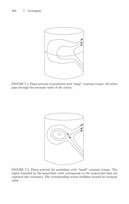
464 7. Averaging
FIGURE 7.1. Phase portrait of pendulum with “large” constant torque. All orbitspass through the resonant value of the action.
FIGURE 7.2. Phase portrait for pendulum with “small” constant torque. Theregion bounded by the homoclinic orbit corresponds to the trajectories that arecaptured into resonance. The corresponding action oscillates around its resonantvalue.
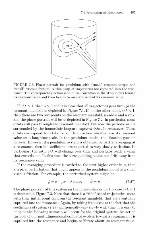
7.2 Averaging at Resonance 465
FIGURE 7.3. Phase portrait for pendulum with “small” constant torque and“small” viscous friction. A thin strip of trajectories are captured into the reso-nance. The corresponding action with initial condition in the strip moves towardits resonant value and then begins to oscillate around its resonant value.
If c/λ > 1, then ρ > 0 and it is clear that all trajectories pass through theresonant manifold as depicted in Figure 7.1. If, on the other hand, c/λ < 1,then there are two rest points on the resonant manifold, a saddle and a sink,and the phase portrait will be as depicted in Figure 7.2. In particular, someorbits still pass through the resonant manifold, but now the periodic orbitssurrounded by the homoclinic loop are captured into the resonance. Theseorbits correspond to orbits for which an action librates near its resonantvalue on a long time scale. In the pendulum model, the libration goes onfor ever. However, if a pendulum system is obtained by partial averaging ata resonance, then its coefficients are expected to vary slowly with time. Inparticular, the ratio c/λ will change over time and perhaps reach a valuethat exceeds one. In this case, the corresponding action can drift away fromits resonance value.
If the averaging procedure is carried to the next higher order in µ, thena typical perturbation that might appear in the pendulum model is a smallviscous friction. For example, the perturbed system might be
ρ = c − µρ − λ sin ψ, ψ = ρ. (7.27)
The phase portrait of this system on the phase cylinder for the case c/λ < 1is depicted in Figure 7.3. Note that there is a “thin” set of trajectories, somewith their initial point far from the resonant manifold, that are eventuallycaptured into the resonance. Again, by taking into account the fact that thecoefficients of system (7.27) will generally vary slowly with time, it is easy toimagine the following scenario will occur for the original system: An actionvariable of our multidimensional oscillator evolves toward a resonance, it iscaptured into the resonance and begins to librate about its resonant value.
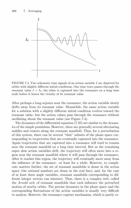
466 7. Averaging
t
I
I
FIGURE 7.4. Two schematic time signals of an action variable I are depicted fororbits with slightly different initial conditions. One time trace passes through theresonant value I = I0; the other is captured into the resonance on a long timescale before it leaves the vicinity of its resonant value.
After perhaps a long sojourn near the resonance, the action variable slowlydrifts away from its resonant value. Meanwhile, the same action variablefor a solution with a slightly different initial condition evolves toward theresonant value, but the action values pass through the resonance withoutoscillating about the resonant value (see Figure 7.4).
The dynamics of the differential equation (7.25) are similar to the dynam-ics of the simple pendulum. However, there are generally several alternatingsaddles and centers along the resonant manifold. Thus, for a perturbationof this system, there can be several “thin” subsets of the phase space cor-responding to trajectories that are eventually captured into the resonance.Again trajectories that are captured into a resonance will tend to remainnear the resonant manifold on a long time interval. But as the remainingsuper slow action variables drift, the trajectory will often move into a re-gion near the resonant manifold where it will pass through the resonance.After it reaches this region, the trajectory will eventually move away fromthe influence of the resonance—at least for a while. However, to compli-cate matters further, the set of resonant manifolds is dense in the actionspace (the rational numbers are dense in the real line); and, for the caseof at least three angle variables, resonant manifolds corresponding to dif-ferent integer vectors can intersect. Thus, there is a complex web, calledthe Arnold web, of resonant manifolds that each influence the perturbedmotion of nearby orbits. The precise dynamics in the phase space and thecorresponding fluctuations of the action variables is usually very difficultto analyze. However, the resonance capture mechanism, which is partly re-
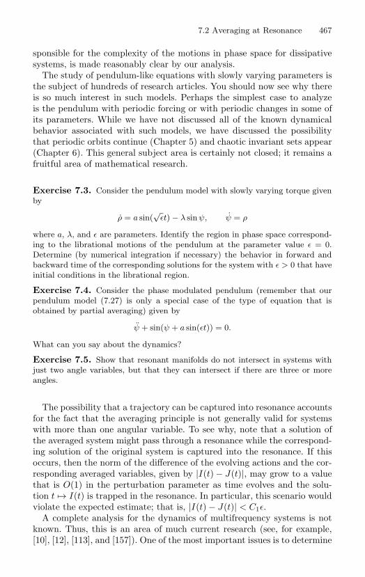
7.2 Averaging at Resonance 467
sponsible for the complexity of the motions in phase space for dissipativesystems, is made reasonably clear by our analysis.
The study of pendulum-like equations with slowly varying parameters isthe subject of hundreds of research articles. You should now see why thereis so much interest in such models. Perhaps the simplest case to analyzeis the pendulum with periodic forcing or with periodic changes in some ofits parameters. While we have not discussed all of the known dynamicalbehavior associated with such models, we have discussed the possibilitythat periodic orbits continue (Chapter 5) and chaotic invariant sets appear(Chapter 6). This general subject area is certainly not closed; it remains afruitful area of mathematical research.
Exercise 7.3. Consider the pendulum model with slowly varying torque givenby
ρ = a sin(√
εt) − λ sin ψ, ψ = ρ
where a, λ, and ε are parameters. Identify the region in phase space correspond-ing to the librational motions of the pendulum at the parameter value ε = 0.Determine (by numerical integration if necessary) the behavior in forward andbackward time of the corresponding solutions for the system with ε > 0 that haveinitial conditions in the librational region.
Exercise 7.4. Consider the phase modulated pendulum (remember that ourpendulum model (7.27) is only a special case of the type of equation that isobtained by partial averaging) given by
ψ + sin(ψ + a sin(εt)) = 0.
What can you say about the dynamics?
Exercise 7.5. Show that resonant manifolds do not intersect in systems withjust two angle variables, but that they can intersect if there are three or moreangles.
The possibility that a trajectory can be captured into resonance accountsfor the fact that the averaging principle is not generally valid for systemswith more than one angular variable. To see why, note that a solution ofthe averaged system might pass through a resonance while the correspond-ing solution of the original system is captured into the resonance. If thisoccurs, then the norm of the difference of the evolving actions and the cor-responding averaged variables, given by |I(t) − J(t)|, may grow to a valuethat is O(1) in the perturbation parameter as time evolves and the solu-tion t → I(t) is trapped in the resonance. In particular, this scenario wouldviolate the expected estimate; that is, |I(t) − J(t)| < C1ε.
A complete analysis for the dynamics of multifrequency systems is notknown. Thus, this is an area of much current research (see, for example,[10], [12], [113], and [157]). One of the most important issues is to determine
468 7. Averaging
the “diffusion rates” for the actions to leave the vicinity of a resonance andto arrive at a second resonance. The long term stability of the models of themotion of many-body systems, for example our solar system, is essentiallybound up with this question. This is currently one of the great unsolvedproblems in mathematics.
A concrete counterexample to the validity of averaging for the case oftwo or more angles is provided by the system
I1 = ε,
I2 = ε cos(θ2 − θ1),θ1 = I1,
θ2 = I2, (7.28)
introduced in [157] (see Exercise 7.6).
Exercise 7.6. Find the averaged system for the oscillator (7.28) and the gen-eral analytical solution of the averaged system. Show that a solution of the orig-inal system is given by
I1(t) = εt + I0,
I2(t) = I1(t),
θ1(t) = ε12t2 + I0t + θ1(0),
θ2(t) = θ1(t).
For these solutions, show that the estimate expected from the averaging theorem(Theorem 7.2) is not valid.
Let us note that system (7.28) has a resonant manifold given by theresonance relation I2 −I1 = 0. As prescribed above in our partial averagingprocedure, consider new coordinates defined by
√ε ρ = I2 − I1, z = I2, ψ = θ2 − θ1, χ = θ2,
and note that system (7.28), when expressed in these coordinates, is givenby
ρ =√
ε (cos ψ − 1),z = ε cos ψ,
ψ =√
ε ρ,
χ = z. (7.29)
7.2 Averaging at Resonance 469
Averaging over the fast angle χ in system (7.29) produces the partiallyaveraged system
˙ρ =√
ε (cos ψ − 1),˙z = 0,
˙ψ =√
ε ρ. (7.30)
For each fixed z, there is an orbit O1 whose ω-limit set is the rest point(ρ, z, ψ) = (0, z, 0) and a second orbit O2 with this rest point as its α-limitset. (Prove this!) The trajectories corresponding to the orbit O1 are allcaptured into the resonance relative to the first order approximation of thepartially averaged system, and the rest point is captured for all time. Butthe action corresponding to z, a super slow variable, drifts from its initialvalue so that the trajectories corresponding to the orbit O1 eventually passthrough the resonance. This example thus provides a clear illustration of themechanism that destroys the possibility that the averaged system—not thepartially averaged system—gives a good approximation to the full systemover a long time scale. In effect, the averaged system for this example doesnot “feel the influence of the resonance.”
Exercise 7.7. The partially averaged system (7.30) is obtained by averagingover just one angle. Thus, the averaging theorem ensures that under appropriaterestrictions the partially averaged system is a good approximation to the originalsystem. Formulate appropriate restrictions on the domain of definition of thepartially averaged system and determine an appropriate time scale for the validityof averaging. Give a direct proof that your formulation is valid.
Exercise 7.8. In applied mathematics, often only the lowest order resonancesare considered; they seem to have the most influence on the dynamics. As anexample to illustrate why this observation might be justified, consider the nearresonance dynamics of system (7.28) at a “high” order resonance given by theresonance relation mI1 = nI2 where m and n are relatively prime, and m = n.Show that there are integers k and such that the matrix
R :=(
m −nk
)
is unimodular. Next, define new angular coordinates by(φ1
φ2
)= R
(θ1
θ2
).
Also, define new action variables by√
ε ρ = mI1 − nI2, z = kI1 + I2.
Change to the new coordinates, find the partially averaged system, and showthat, in this approximation, all orbits pass through the resonance. Does thismean that the averaging principle is valid for orbits starting near the higherorder resonances in this example?
470 7. Averaging
Let us consider the system (7.1) with u ∈ R2; that is, a planar period-
ically perturbed oscillator. Furthermore, let us assume that action-anglevariables have been introduced—in this case, the resonant invariant man-ifold given by the resonance relation mω(I) = nΩ is a point I = I0 in theone-dimensional action space.
In order to find the partially averaged system at the resonant layer givenby I = I0, let ρ denote the scaled distance to the resonant manifold; thatis,
√ε ρ = I − I0.
Also, let τ = Ωt, and introduce a new angular variable by
ψ = mφ − nτ.
Then, to first order in the perturbation parameter√
ε, the differential equa-tion in these new coordinates is given by the system
ρ =√
ε F (I0, ψ/m + nτ/m, τ/Ω) + O(ε),ψ =
√ε mω′(I0)ρ + O(ε),
τ = Ω.
Whereas the variables ρ and ψ are slow variables, τ , corresponding to thetime variable in our nonautonomous perturbation, is a single fast angularvariable. By the averaging theorem, there is a change of coordinates suchthat the transformed system, to leading order in µ =
√ε, is given by
J = µF (θ), θ = µmω′(I0)J (7.31)
where
F (θ) :=1
2πm
∫ 2πm
0F (I0, θ/m + nτ/m, τ/Ω) dτ.
Under the assumption that ω′(I0) = 0—in other words, under the as-sumption that the unperturbed resonant periodic orbit corresponding tothe action I = I0 is normally nondegenerate—the averaged system forε > 0 has a nondegenerate rest point at (J0, θ0) if and only if J0 = 0 andthe function F has θ0 as a simple zero.
Note that the solution of the system
J = µF (θ), θ = µmω′(I0)J, τ = Ω
starting at the point (J, θ, τ) = (0, θ0, 0) is a periodic orbit, and in addi-tion if the rest point is hyperbolic, then this periodic orbit is hyperbolic.We would like to conclude that there is a corresponding periodic orbit forthe original oscillator. This fact is implied by the following more generaltheorem.
7.2 Averaging at Resonance 471
Theorem 7.9. Consider the system
I = εF (I, θ) + ε2F2(I, θ, ε),θ = ω(I) + εG(I, θ, ε) (7.32)
where I ∈ RM and θ ∈ T, where F , F2, and G are 2π-periodic functions
of θ, and where there is some number c such that ω(I) > c > 0. If theaveraged system has a nondegenerate rest point, then for sufficiently smallε system (7.32) has a periodic orbit. If in addition ε > 0 and the restpoint is hyperbolic, then the periodic orbit has the same stability type asthe hyperbolic rest point; that is, the dimensions of the corresponding stableand unstable manifolds are the same.
Proof. The averaged differential equation is given by J = εF (J) whereF is the average of the function θ → F (I, θ). Let us suppose that J0 is anondegenerate rest point of the averaged system; that is, F (J0) = 0 andthe derivative DF (J0) is an invertible transformation.
By the averaging theorem, if ε is sufficiently small, then there is a 2π-periodic change of coordinates of the form J = I + εL(I, θ), defined inan open set containing J0 × T, such that system (7.32) in these newcoordinates is given by
J = εF (J) + O(ε2),θ = ω(J) + O(ε). (7.33)
Let t → (J(t, ξ, ε), θ(t, ξ, ε)) denote the solution of the system (7.33)such that J(0, ξ, ε) = ξ and θ(0, ξ, ε) = 0. By an application of the implicitfunction theorem, there is a smooth function (ξ, ε) → T (ξ, ε) that is definedin a neighborhood of (J, θ) = (J0, 0) such that T (J0, 0) = 2π/ω(J0) andθ(T (ξ, ε), ξ, ε) ≡ 2π. Moreover, let us define a (parametrized) Poincare mapwith the same domain as the transit time map T by
P (ξ, ε) := J(T (ξ, ε), ξ, ε).
By expanding the function ε → P (ξ, ε) into a Taylor series at ε = 0, weobtain
P (ξ, ε) = J(T (ξ, 0), ξ, 0) + ε(J(T (ξ, 0), ξ, 0)Tε(ξ, 0)+ Jε(T (ξ, 0), ξ, 0)) + O(ε2).
Note that J(T (ξ, 0), ξ, 0) ≡ ξ and J(T (ξ, 0), ξ, 0) = 0. Moreover, the func-tion t → Jε(t, ξ, 0) is the solution of the variational initial value problemgiven by
W = F (J(t, ξ, 0)), W (0) = 0.
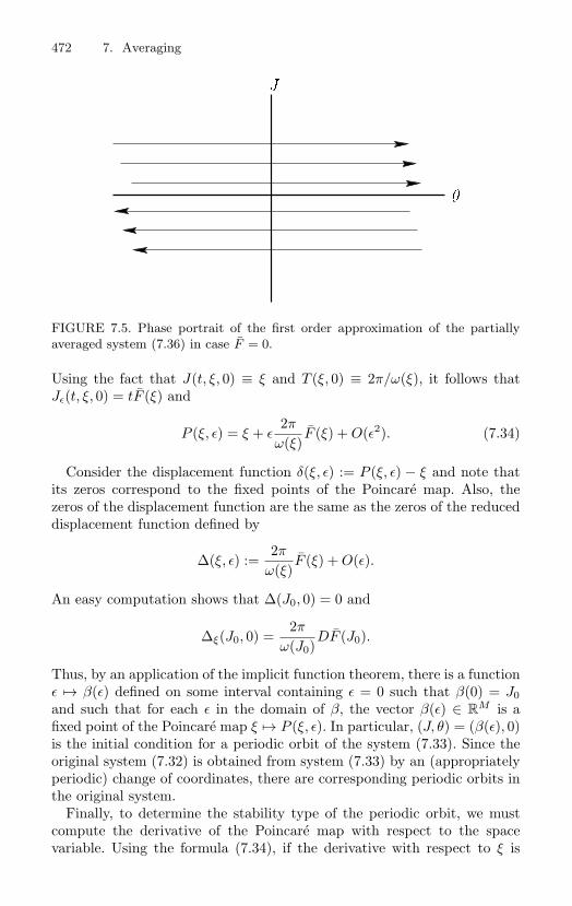
472 7. Averaging
J
FIGURE 7.5. Phase portrait of the first order approximation of the partiallyaveraged system (7.36) in case F = 0.
Using the fact that J(t, ξ, 0) ≡ ξ and T (ξ, 0) ≡ 2π/ω(ξ), it follows thatJε(t, ξ, 0) = tF (ξ) and
P (ξ, ε) = ξ + ε2π
ω(ξ)F (ξ) + O(ε2). (7.34)
Consider the displacement function δ(ξ, ε) := P (ξ, ε) − ξ and note thatits zeros correspond to the fixed points of the Poincare map. Also, thezeros of the displacement function are the same as the zeros of the reduceddisplacement function defined by
∆(ξ, ε) :=2π
ω(ξ)F (ξ) + O(ε).
An easy computation shows that ∆(J0, 0) = 0 and
∆ξ(J0, 0) =2π
ω(J0)DF (J0).
Thus, by an application of the implicit function theorem, there is a functionε → β(ε) defined on some interval containing ε = 0 such that β(0) = J0and such that for each ε in the domain of β, the vector β(ε) ∈ R
M is afixed point of the Poincare map ξ → P (ξ, ε). In particular, (J, θ) = (β(ε), 0)is the initial condition for a periodic orbit of the system (7.33). Since theoriginal system (7.32) is obtained from system (7.33) by an (appropriatelyperiodic) change of coordinates, there are corresponding periodic orbits inthe original system.
Finally, to determine the stability type of the periodic orbit, we mustcompute the derivative of the Poincare map with respect to the spacevariable. Using the formula (7.34), if the derivative with respect to ξ is
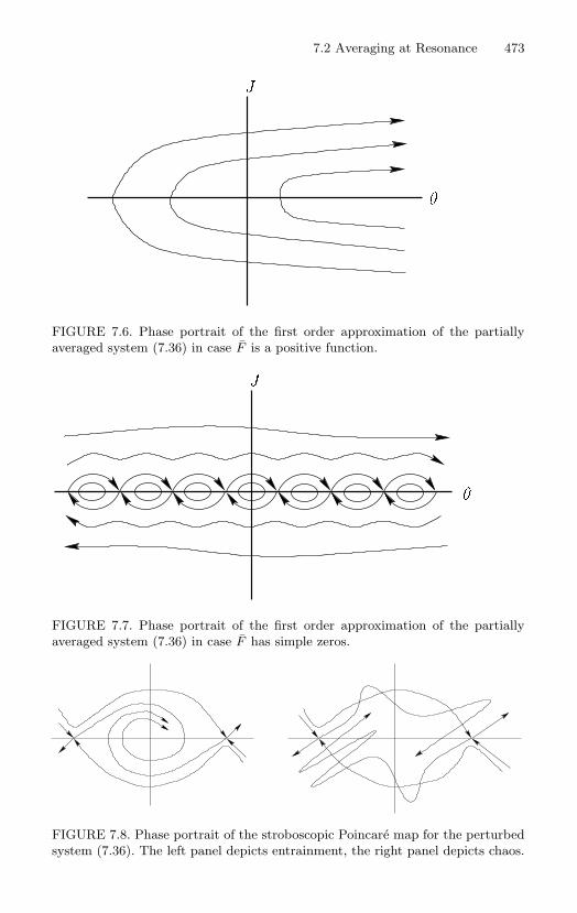
7.2 Averaging at Resonance 473
J
FIGURE 7.6. Phase portrait of the first order approximation of the partiallyaveraged system (7.36) in case F is a positive function.
J
FIGURE 7.7. Phase portrait of the first order approximation of the partiallyaveraged system (7.36) in case F has simple zeros.
FIGURE 7.8. Phase portrait of the stroboscopic Poincare map for the perturbedsystem (7.36). The left panel depicts entrainment, the right panel depicts chaos.
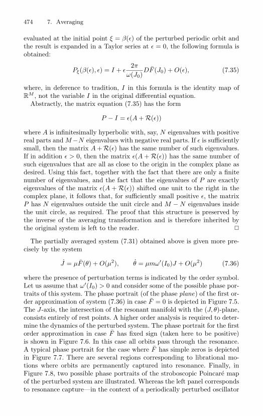
474 7. Averaging
evaluated at the initial point ξ = β(ε) of the perturbed periodic orbit andthe result is expanded in a Taylor series at ε = 0, the following formula isobtained:
Pξ(β(ε), ε) = I + ε2π
ω(J0)DF (J0) + O(ε), (7.35)
where, in deference to tradition, I in this formula is the identity map ofR
M , not the variable I in the original differential equation.Abstractly, the matrix equation (7.35) has the form
P − I = ε(A + R(ε))
where A is infinitesimally hyperbolic with, say, N eigenvalues with positivereal parts and M −N eigenvalues with negative real parts. If ε is sufficientlysmall, then the matrix A + R(ε) has the same number of such eigenvalues.If in addition ε > 0, then the matrix ε(A + R(ε)) has the same number ofsuch eigenvalues that are all as close to the origin in the complex plane asdesired. Using this fact, together with the fact that there are only a finitenumber of eigenvalues, and the fact that the eigenvalues of P are exactlyeigenvalues of the matrix ε(A + R(ε)) shifted one unit to the right in thecomplex plane, it follows that, for sufficiently small positive ε, the matrixP has N eigenvalues outside the unit circle and M − N eigenvalues insidethe unit circle, as required. The proof that this structure is preserved bythe inverse of the averaging transformation and is therefore inherited bythe original system is left to the reader.
The partially averaged system (7.31) obtained above is given more pre-cisely by the system
J = µF (θ) + O(µ2), θ = µmω′(I0)J + O(µ2) (7.36)
where the presence of perturbation terms is indicated by the order symbol.Let us assume that ω′(I0) > 0 and consider some of the possible phase por-traits of this system. The phase portrait (of the phase plane) of the first or-der approximation of system (7.36) in case F = 0 is depicted in Figure 7.5.The J-axis, the intersection of the resonant manifold with the (J, θ)-plane,consists entirely of rest points. A higher order analysis is required to deter-mine the dynamics of the perturbed system. The phase portrait for the firstorder approximation in case F has fixed sign (taken here to be positive)is shown in Figure 7.6. In this case all orbits pass through the resonance.A typical phase portrait for the case where F has simple zeros is depictedin Figure 7.7. There are several regions corresponding to librational mo-tions where orbits are permanently captured into resonance. Finally, inFigure 7.8, two possible phase portraits of the stroboscopic Poincare mapof the perturbed system are illustrated. Whereas the left panel correspondsto resonance capture—in the context of a periodically perturbed oscillator
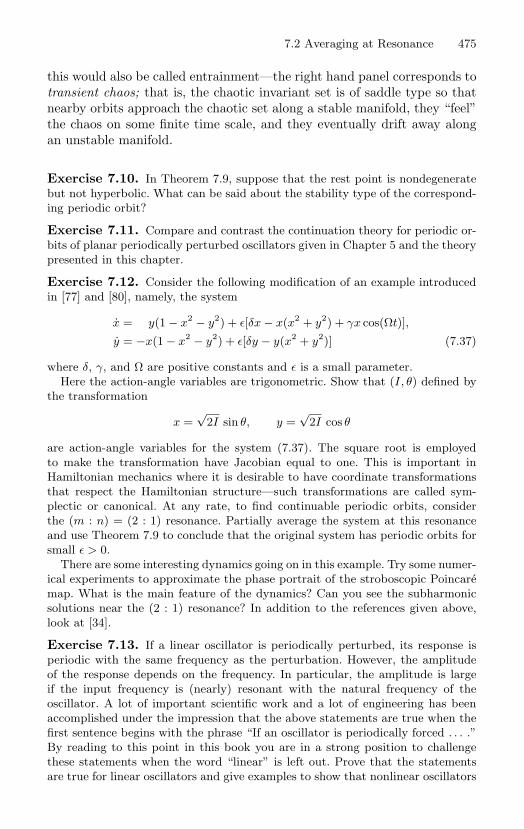
7.2 Averaging at Resonance 475
this would also be called entrainment—the right hand panel corresponds totransient chaos; that is, the chaotic invariant set is of saddle type so thatnearby orbits approach the chaotic set along a stable manifold, they “feel”the chaos on some finite time scale, and they eventually drift away alongan unstable manifold.
Exercise 7.10. In Theorem 7.9, suppose that the rest point is nondegeneratebut not hyperbolic. What can be said about the stability type of the correspond-ing periodic orbit?
Exercise 7.11. Compare and contrast the continuation theory for periodic or-bits of planar periodically perturbed oscillators given in Chapter 5 and the theorypresented in this chapter.
Exercise 7.12. Consider the following modification of an example introducedin [77] and [80], namely, the system
x = y(1 − x2 − y2) + ε[δx − x(x2 + y2) + γx cos(Ωt)],
y = −x(1 − x2 − y2) + ε[δy − y(x2 + y2)] (7.37)
where δ, γ, and Ω are positive constants and ε is a small parameter.Here the action-angle variables are trigonometric. Show that (I, θ) defined by
the transformation
x =√
2I sin θ, y =√
2I cos θ
are action-angle variables for the system (7.37). The square root is employedto make the transformation have Jacobian equal to one. This is important inHamiltonian mechanics where it is desirable to have coordinate transformationsthat respect the Hamiltonian structure—such transformations are called sym-plectic or canonical. At any rate, to find continuable periodic orbits, considerthe (m : n) = (2 : 1) resonance. Partially average the system at this resonanceand use Theorem 7.9 to conclude that the original system has periodic orbits forsmall ε > 0.
There are some interesting dynamics going on in this example. Try some numer-ical experiments to approximate the phase portrait of the stroboscopic Poincaremap. What is the main feature of the dynamics? Can you see the subharmonicsolutions near the (2 : 1) resonance? In addition to the references given above,look at [34].
Exercise 7.13. If a linear oscillator is periodically perturbed, its response isperiodic with the same frequency as the perturbation. However, the amplitudeof the response depends on the frequency. In particular, the amplitude is largeif the input frequency is (nearly) resonant with the natural frequency of theoscillator. A lot of important scientific work and a lot of engineering has beenaccomplished under the impression that the above statements are true when thefirst sentence begins with the phrase “If an oscillator is periodically forced . . . .”By reading to this point in this book you are in a strong position to challengethese statements when the word “linear” is left out. Prove that the statementsare true for linear oscillators and give examples to show that nonlinear oscillators
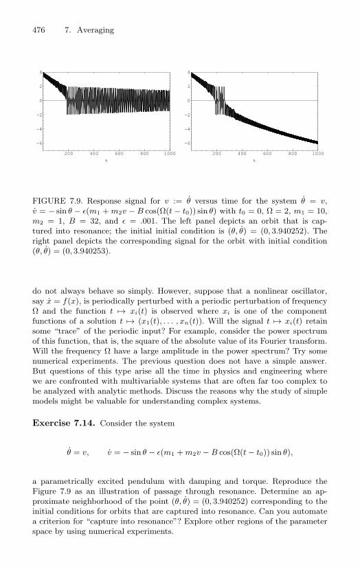
476 7. Averaging
200 400 600 800 1000
t
-6
-4
-2
0
2
4
200 400 600 800 1000
t
-6
-4
-2
0
2
4
FIGURE 7.9. Response signal for v := θ versus time for the system θ = v,v = − sin θ − ε(m1 + m2v − B cos(Ω(t − t0)) sin θ) with t0 = 0, Ω = 2, m1 = 10,m2 = 1, B = 32, and ε = .001. The left panel depicts an orbit that is cap-tured into resonance; the initial initial condition is (θ, θ) = (0, 3.940252). Theright panel depicts the corresponding signal for the orbit with initial condition(θ, θ) = (0, 3.940253).
do not always behave so simply. However, suppose that a nonlinear oscillator,say x = f(x), is periodically perturbed with a periodic perturbation of frequencyΩ and the function t → xi(t) is observed where xi is one of the componentfunctions of a solution t → (x1(t), . . . , xn(t)). Will the signal t → xi(t) retainsome “trace” of the periodic input? For example, consider the power spectrumof this function, that is, the square of the absolute value of its Fourier transform.Will the frequency Ω have a large amplitude in the power spectrum? Try somenumerical experiments. The previous question does not have a simple answer.But questions of this type arise all the time in physics and engineering wherewe are confronted with multivariable systems that are often far too complex tobe analyzed with analytic methods. Discuss the reasons why the study of simplemodels might be valuable for understanding complex systems.
Exercise 7.14. Consider the system
θ = v, v = − sin θ − ε(m1 + m2v − B cos(Ω(t − t0)) sin θ),
a parametrically excited pendulum with damping and torque. Reproduce theFigure 7.9 as an illustration of passage through resonance. Determine an ap-proximate neighborhood of the point (θ, θ) = (0, 3.940252) corresponding to theinitial conditions for orbits that are captured into resonance. Can you automatea criterion for “capture into resonance”? Explore other regions of the parameterspace by using numerical experiments.
7.3 Action-Angle Variables 477
7.3 Action-Angle Variables
To use the theory presented so far in this chapter we must be able toexpress our oscillator in action-angle variables. In practice, the constructionof action-angle variables is a formidable task—recall the construction ofthe Delaunay variables in Chapter 3. For linear oscillators the appropriatecoordinate change can be constructed using polar coordinates, while theconstruction of action-angle variables for the pendulum requires the use ofJacobi elliptic functions. A general construction of action angle-variablesfor planar oscillators is presented in this section. The construction usessome of the ideas discussed in Chapter 5.
Let us consider a differential equation of the form
u = f(u) + εg(u, t)
where the unperturbed system
u = f(u) (7.38)
has a period annulus A. We will construct action-angle variables near aperiodic orbit Γ contained in A. The differential equation (7.38), expressedin the new coordinates that we denote by I and ϑ, has the form
I = 0, ϑ = ω(I).
Interpreted geometrically, these new coordinates are related to polar co-ordinates in that I is a radial variable and ϑ is an angular variable. Infact, whereas I is constant on each periodic solution, ϑ changes linearly oneach periodic solution. In case the system (7.38) is Hamiltonian, the newcoordinates reduce to the usual action-angle variables on A.
With reference to system (7.38), define the orthogonal system
u = f⊥(u), u ∈ X (7.39)
where, in oriented local coordinates, f⊥(u) := Jf(u) with
J =(
0 −11 0
).
We mention that J rotates vectors in the plane through a positive angleof π/2 radians. The same symbol J is often used in this context with theopposite sign.
Let ϕt denote the flow of the differential equation (7.38) and let ψt denotethe flow of the differential equation (7.39). Also, for vectors ξ1 and ξ2 inR
2, define ξ1 ∧ ξ2 := 〈ξ1, Jξ2〉, where the brackets denote the usual innerproduct in R
2.A periodic orbit Γ of (7.38) has an orientation determined by its time
parameterization. To specify an orientation, we define ε = ε(f) = 1 in case
478 7. Averaging
for each ζ ∈ Γ the vector f⊥(ζ) is the outer normal at ζ. If f⊥(ζ) is theinner normal, then ε := −1. Also, the orientation of the period annulusA is defined to be the orientation inherited from its constituent periodicsolutions.
Choose a point ζ ∈ A and note that there is an open interval U ⊂ R
containing the origin such that the image of the map ρ → ψρ(ζ) for ρ ∈ Uis a section Σζ transverse to the orbits of system (7.38) in A. Also, defineΥ : U × R → A by
Υ(ρ, φ) = ϕφ(ψρ(ζ)). (7.40)
Clearly, Υ is smooth. In fact, Υ is a covering map, that is, a periodic coordi-nate system on A. We will see below that Υ defines “flow box” coordinates:coordinates that straighten out the flow in a neighborhood of the periodicorbit containing the point ζ.
To construct the action-angle variables, let us begin by considering thederivative of the map Υ defined in display (7.40). Diliberto’s theorem (The-orem 5.5) states that if
b(t, ζ) :=||f(ζ)||2
||f(ϕt(ζ))||2 e∫ t0 div f(ϕs(v)) ds,
a(t, ζ) :=∫ t
0
(2κ(s, ζ)||f(ϕs(ζ))|| − curl f(ϕs(ζ))
)b(s, ζ) ds, (7.41)
where κ denotes the signed scalar curvature along the curve t → ϕt(ζ),ζ ∈ A, then
DΥ(ρ, φ)∂
∂φ= f(Υ(ρ, φ)),
DΥ(ρ, φ)∂
∂ρ= b(φ, ψρ(v))f⊥(Υ(ρ, φ)) + a(φ, ψρ(v))f(Υ(ρ, φ)).
In other words, the matrix representation of the derivative DΥ(ρ, φ) relativeto the ordered bases ∂/∂ρ, ∂/∂φ and f⊥(Υ(ρ, φ)), f(Υ(ρ, φ)) is givenby
DΥ(ρ, φ) =(
b(φ, ψρ(v)) 0a(φ, ψρ(v)) 1
).
Since b does not vanish for ζ ∈ A, it follows that Υ is a local diffeomorphismand in fact Υ is a covering map onto its image.
To express the original system (7.38) in (ρ, φ)-coordinates, note first thatthere are smooth functions (u, t) → p(u, t) and (u, t) → q(u, t) such that
g(u, t) = p(u, t)f⊥(u) + q(u, t)f(u) (7.42)
for all (u, t) ∈ A×R. Thus, to change system (7.38) to the new coordinates,we simply solve for
j(u, t)∂
∂ρ+ k(u, t)
∂
∂φ
7.3 Action-Angle Variables 479
in the matrix equation (b 0a 1
)(jk
)=
(εp
1 + εq
)to obtain (
jk
)=
(ε 1
b p1 + ε(q − a
b p)
).
It follows that system (7.38) in the new coordinates is given by
ρ = ε1
b(φ, ψρ(v))p(Υ(ρ, φ), t),
φ = 1 + ε(q(Υ(ρ, φ), t) − a(φ, ψρ(v))
b(φ, ψρ(v))p(Υ(ρ, φ), t)
). (7.43)
To compress notation, let us write (7.43) in the form
ρ = εQ(ρ, φ, t), φ = 1 + εR(ρ, φ, t). (7.44)
Define a second change of coordinates by
ρ = β(I), φ = α(I)ϑ (7.45)
where I → α(I) and I → β(I) are smooth functions to be specified below.Here, since the coordinate transformation must be invertible, we need onlyassume that α(I)β′(I) = 0. In the (I, ϑ)-coordinates, system (7.43) has theform
I = ε1
β′(I)Q(β(I), α(I)ϑ, t),
ϑ =φ − ϑα′(I)I
α(I)(7.46)
=1
α(I)+ ε
( 1α(I)
R(β(I), α(I)ϑ, t) − ϑα′(I)
α(I)β′(I)Q(β(I), α(I)ϑ, t)
).
To specify the functions α and β we require two auxiliary functions—the period function and the area function. To define the period function,recall that the image of the map ρ → ψρ(ζ) for ρ ∈ U is a section forthe unperturbed flow on the period annulus A. The period function on Arelative to this section is the map T : U → R that assigns to each ρ ∈ Uthe minimum period of the solution of system (7.38) that passes throughthe point φρ(ζ) ∈ A. In the “standard” case, A is an annulus whose innerboundary is a rest point. In this case, we define the area function ζ → A(ζ);it assigns to each ζ ∈ A the area enclosed by the unperturbed solutionthrough ζ.
480 7. Averaging
The function β is defined to be the solution of the initial value problem
dρ
dI= ε
2π
T (ρ)
1||f(ψρ(ζ))||2 , ρ(I0) = 0 (7.47)
where in the standard case I0 = A(ζ)/(2π), and in the case where A hasa nontrivial inner boundary I0 = 0. The choice of initial condition for thestandard case agrees with tradition. However, a different choice of initialcondition simply results in a constant translation of the “action” variable.The function α is defined by
α(I) := −εT (β(I))
2π(7.48)
where ε = ±1 according to the orientation of the period annulus A.Using the definition T (I) := T (β(I)), the system (7.46) has the form
I = εεT (I)2π
||f(ψρ(ζ))||2Q(β(I), α(I)ϑ, t),
ϑ = −ε2π
T (I)− εε
( 2π
T (I)R(β(I), α(I)ϑ, t)
+ ϑT ′(I)2π
||f(ψρ(ζ))||2Q(β(I), α(I)ϑ, t)). (7.49)
From equation (7.42), we have the identities
p =1
||f ||2 〈g, f⊥〉 =1
||f ||2 f ∧ g, q =1
||f ||2 〈f, g〉.
Thus, in view of system (7.43) the system (7.49) can be rewritten in theform
I = εεT (I)2π
E(I, ϑ)f(Υ(β(I), α(I)ϑ)) ∧ g(Υ(β(I), α(I)ϑ), t),
ϑ = −ε2π
T (I)
− εε[ 2π
T (I)||f(Υ(β(I), α(I)ϑ))||−2〈f, g〉 +
(ϑ
T ′(I)2π
||f(ψβ(I)(ζ))||2
− 2π
T (I)a(α(I)ϑ, ψβ(I)(ζ))
)||f(φβ(I)(ζ))||−2E(I, ϑ)f ∧ g
](7.50)
where
E(I, ϑ) := e− ∫ α(I)ϑ0 div f(Υ(β(I),α(I)s)) ds.
Again, for notational convenience, let us write the first order system (7.50)in the compact form
I = εF (I, ϑ, t), ϑ = ω(I) + εG(I, ϑ). (7.51)
7.3 Action-Angle Variables 481
Note that both F and G are 2π-periodic in ϑ and 2π/Ω-periodic in t.Thus, we have transformed the original perturbed system to action-anglecoordinates.
To prove that the action-angle coordinate transformation
u = Υ(β(I), α(I)ϑ) (7.52)
is canonical in case the unperturbed system is Hamiltonian, it suffices toshow the transformation is area preserving, that is, the Jacobian of thetransformation is unity. In fact, the Jacobian is
det[(
−f2(u) f1(u)f1(u) f2(u)
)(a(φ, ψρ(ζ)) 1
)(β′(I) 0α′(I)ϑ α(I)
)]=
||f(u)||2||f(ψρ(ζ))||2 b(φ, ψρ(ζ)).
But, if f is a Hamiltonian vector field, then div f = 0, and
b(φ, ψρ(ζ)) =||f(ψρ(ζ))||2
||f(u)||2 ,
as required. Moreover, in case f is the Hamiltonian vector field for theHamiltonian H, we have f(u) = −J gradH(u). Recall that ρ = β(I) anddefine h := H(ψρ(ζ)). Then,
dI
dh= ε
T (ρ(h))2π
.
Thus, the derivative of the action with respect to energy is the normalizedenergy-period function, as it should be.
8Local Bifurcation
Consider the family of differential equations
u = f(u, ε), u ∈ Rn, ε ∈ R. (8.1)
If f(u0, ε0) = 0, then the differential equation with parameter value ε = ε0has a rest point at u0 and the linearized system at this point is given by
W = fu(u0, ε0)W. (8.2)
If the eigenvalues of the linear transformation fu(u0, ε0) : Rn → R
n areall nonzero, then the transformation is invertible, and by an application ofthe implicit function theorem there is a curve ε → β(ε) in R
n such thatβ(ε0) = u0 and f(β(ε), ε) ≡ 0. In other words, for each ε in the domain ofβ the point β(ε) ∈ R
n corresponds to a rest point for the member of thefamily (8.1) at the parameter value ε.
Recall that if all eigenvalues of the linear transformation fu(u0, ε0) havenonzero real parts, then the transformation is called infinitesimally hyper-bolic and the rest point u0 is called hyperbolic. Also, in this case, since theeigenvalues of Df(u, ε) depend continuously on u and the parameter ε, if|ε − ε0| is sufficiently small, then the rest point u = β(ε) of the differentialequation (8.1) at the parameter value ε has the same stability type as therest point u0 = β(ε0). In particular, if the rest point u0 is hyperbolic, thenfor sufficiently small ε the perturbed rest point β(ε) is also hyperbolic.
If fu(u0, ε0) is not infinitesimally hyperbolic, then there is at least oneeigenvalue with zero real part. It turns out that the topology of the lo-cal phase portrait of the corresponding differential equation (8.1) at this
484 8. Local Bifurcation
rest point may change under perturbation; if it does, we will say that abifurcation occurs. For example, the phase portrait for a nearby differentialequation may have no rest points or several rest points in the vicinity ofthe original rest point. In this chapter, we will consider such bifurcations incase the linear transformation fu(u0, ε0) has a simple zero eigenvalue; thatis, a zero eigenvalue with algebraic (and geometric) multiplicity one, or apair of pure imaginary complex conjugate eigenvalues each with algebraicmultiplicity one, and we will describe some of the “generic” bifurcationsthat occur under these conditions.
While only the loss of stability at a rest point of a differential equationwill be discussed, the basic results presented here can be modified to coverthe case of the loss of stability of a fixed point of a map; and in turn themodified theory can be applied to the Poincare map to obtain a bifurcationtheory for periodic orbits. However, the extension of bifurcation theory fromrest points to periodic orbits is only the beginning of a vast subject thathas been developed far beyond the scope of this book. For example, theloss of stability of a general invariant manifold can be considered. On theother hand, bifurcation theory is by no means complete: Many interestingproblems are unresolved. (See the books [6] and [50] for detailed and wideranging results on bifurcations of planar vector fields, and [9], [49], [74],[75], [80], [117], [163], [184], and [185] for more general bifurcation theory.)
Exercise 8.1. Prove that the eigenvalues of an n × n matrix depend continu-ously on the components of the matrix.
8.1 One-Dimensional State Space
We will consider the most important bifurcation associated with rest pointsof scalar differential equations, namely, the saddle-node bifurcation, to il-lustrate some of the general concepts of bifurcation theory. In addition, wewill see how bifurcation problems arise in applied mathematics.
8.1.1 The Saddle-Node BifurcationConsider the family of differential equations
u = ε − u2, u ∈ R, ε ∈ R (8.3)
and note that if f(u, ε) := ε − u2, then
f(0, 0) = 0, fu(0, 0) = 0, fuu(0, 0) = −2, fε(0, 0) = 1.
Also, the rest points for members of this family are given by ε = u2. Thus,if ε < 0, then there are no rest points; if ε = 0, then there is one rest
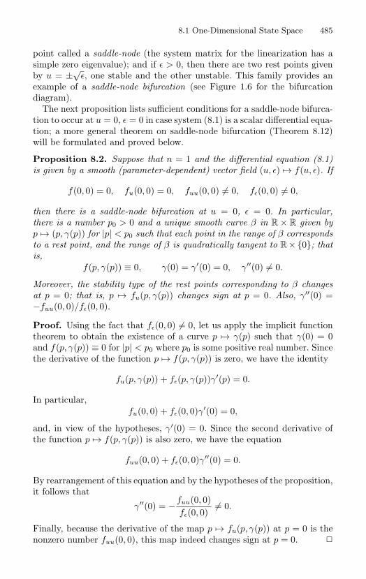
8.1 One-Dimensional State Space 485
point called a saddle-node (the system matrix for the linearization has asimple zero eigenvalue); and if ε > 0, then there are two rest points givenby u = ±
√ε, one stable and the other unstable. This family provides an
example of a saddle-node bifurcation (see Figure 1.6 for the bifurcationdiagram).
The next proposition lists sufficient conditions for a saddle-node bifurca-tion to occur at u = 0, ε = 0 in case system (8.1) is a scalar differential equa-tion; a more general theorem on saddle-node bifurcation (Theorem 8.12)will be formulated and proved below.
Proposition 8.2. Suppose that n = 1 and the differential equation (8.1)is given by a smooth (parameter-dependent) vector field (u, ε) → f(u, ε). If
f(0, 0) = 0, fu(0, 0) = 0, fuu(0, 0) = 0, fε(0, 0) = 0,
then there is a saddle-node bifurcation at u = 0, ε = 0. In particular,there is a number p0 > 0 and a unique smooth curve β in R × R given byp → (p, γ(p)) for |p| < p0 such that each point in the range of β correspondsto a rest point, and the range of β is quadratically tangent to R × 0; thatis,
f(p, γ(p)) ≡ 0, γ(0) = γ′(0) = 0, γ′′(0) = 0.
Moreover, the stability type of the rest points corresponding to β changesat p = 0; that is, p → fu(p, γ(p)) changes sign at p = 0. Also, γ′′(0) =−fuu(0, 0)/fε(0, 0).
Proof. Using the fact that fε(0, 0) = 0, let us apply the implicit functiontheorem to obtain the existence of a curve p → γ(p) such that γ(0) = 0and f(p, γ(p)) ≡ 0 for |p| < p0 where p0 is some positive real number. Sincethe derivative of the function p → f(p, γ(p)) is zero, we have the identity
fu(p, γ(p)) + fε(p, γ(p))γ′(p) = 0.
In particular,fu(0, 0) + fε(0, 0)γ′(0) = 0,
and, in view of the hypotheses, γ′(0) = 0. Since the second derivative ofthe function p → f(p, γ(p)) is also zero, we have the equation
fuu(0, 0) + fε(0, 0)γ′′(0) = 0.
By rearrangement of this equation and by the hypotheses of the proposition,it follows that
γ′′(0) = −fuu(0, 0)fε(0, 0)
= 0.
Finally, because the derivative of the map p → fu(p, γ(p)) at p = 0 is thenonzero number fuu(0, 0), this map indeed changes sign at p = 0.
486 8. Local Bifurcation
8.1.2 A Normal FormIf f satisfies all the hypotheses of Proposition 8.2, then by an applicationof the preparation theorem (Theorem 5.14) this function can be factoredin the form
f(u, ε) = (a0(u) + ε)U(u, ε)
where a0(0) = 0 and U(0, 0) = 0. Thus, the flow of the differential equation
u = f(u, ε) (8.4)
is topologically equivalent to the flow of the differential equation u =a0(u)+ε by the identity homeomorphism. Or, if you like, the two differentialequations are equivalent by a rescaling of time (see Proposition 1.14). More-over, taking into account our hypotheses fu(0, 0) = 0 and fuu(0, 0) = 0, wehave that a′
0(0) = 0 and a′′0(0) = 0. As a result, the function a is given by
a0(u) =12a′′0(0)u2 + O(u3).
By the Morse lemma (Theorem 5.50) there is a change of coordinatesu = µ(y) with µ(0) = 0 that transforms the differential equation (8.4) intothe form
y =1
µ′(y)(ε ± y2)
where, of course, µ′(y) = 0 because the change of coordinates is invertible.By a final rescaling of time and, if necessary, a change in the sign of ε, weobtain the equivalent differential equation
y = ε − y2. (8.5)
The family (8.5) is a normal form for the saddle-node bifurcation: Ev-ery one-parameter family of scalar differential equations that satisfies thehypotheses of Proposition 8.2 at a point of the cross product of the phasespace and the parameter space can be (locally) transformed to this normalform by a (nonlinear) change of coordinates and a rescaling of time. In thiscontext, the differential equation (8.5) is also called a versal deformationor a universal unfolding of the saddle-node.
The reader may suspect that the use of such terms as “versal deforma-tion” and “universal unfolding” is indicative of a rich and mature underly-ing theory. This is indeed the case. Moreover, there are a number of excel-lent books on this subject. For example, the book of Vladimir Arnold [9]has a masterful exposition of the “big ideas” of bifurcation theory while thebooks of Martin Golubitsky and David G. Schaeffer [74] and Golubitsky,Ian Stewart, and Schaeffer [75] contain a more comprehensive study of thesubject (see also [49] and [50]).
In the next two sections we will explore some of the philosophy of bifur-cation theory and discuss how bifurcation problems arise in applied math-ematics.
8.1 One-Dimensional State Space 487
8.1.3 Bifurcation in Applied MathematicsIs bifurcation theory important in applied mathematics? To discuss thisquestion, let us suppose that we have a model of a physical system givenby a family of differential equations that depends on some parameters. Wewill consider the process that might be used to identify these parametersand the value of the resulting model for making physical predictions.
In a typical scenario, a model has “system parameters” and “control pa-rameters.” System parameters specify the measurements of intrinsic physi-cal properties, whereas control parameters correspond to adjustments thatcan be made while maintaining the integrity of the physical system. Bychanging the control parameters in the mathematical model, we can makepredictions so as to avoid expensive physical experiments. Also, we can ex-plore the phenomena that occur over the range of the control parameters.
Ideally, system parameters are identified by comparing predictions of themodel with experimental data. However, for a realistic model with severalsystem parameters, the parameter identification will almost always requirea complicated analysis. In fact, parameter identification is itself a fascinat-ing and important problem in applied mathematics that is not completelysolved. However, let us simply note that the parameter identification pro-cess will not be exact. Indeed, if an approximation algorithm is combinedwith experimental data, then some uncertainty is inevitable.
Suppose the model system of differential equations that we obtain fromour parameter identification process contains a degenerate rest point forsome choices of the control parameters. Have we just been unlucky? Can weadjust the parameters to avoid the degeneracy? What does the appearanceof a degenerate rest point tell us about our original model?
Let us first consider the case where there are no control parameters. If,for example, our original model is given by the differential equation (8.5)and our parameter identification process results in specifying the systemparameter value ε = 0 so that the corresponding differential equation has adegenerate rest point, then it would seem that we have been very unlucky.Indeed, predictions from the model with ε = 0 would seem to be quiteunreliable. By an arbitrarily small change in the estimated value of thesystem parameter, we can construct a model differential equation with twohyperbolic rest points or no rest points at all. The choice ε = 0 for thesystem parameter produces a model that is not structurally stable. On theother hand, by arbitrarily small changes of the system parameter, we canproduce two structurally stable models with completely different qualitativebehavior (see Exercise 8.3).
Clearly, it is important to know if the choice of system parameters pro-duces a structurally unstable model or a model that is “close” to one thatis structurally unstable; if this is the case, then it is important to analyzethe qualitative behavior of the models that are produced by small changesin the system parameters. Whereas in the scalar model (8.5) the analysis
488 8. Local Bifurcation
is transparent, it is not at all obvious how we might detect such struc-tural instabilities in a multiparameter or multidimensional model. On theother hand, because system parameters are viewed as fixed once they areidentified, we can theoretically avoid the structural instabilities by simplyreassigning the system parameters.
For the record, two vector fields defined on the same state space are calledtopologically equivalent if there is a homeomorphism of the state space thatmaps all orbits of the first vector field onto orbits of the second vectorfield, and preserves the direction of time along all the orbits (the timeparameterization of the orbits is ignored). Of course, if two vector fieldsare topologically equivalent, then their phase portraits are qualitatively thesame. A vector field (and the corresponding differential equation) is calledstructurally stable if there is an open set of vector fields in the C1 topologythat contains the given vector field, and all vector fields in this open setare topologically equivalent to the given vector field. The idea is that thetopological type of a structurally stable vector field is not destroyed by asmall smooth perturbation (recall Exercise 1.73).
While it might seem reasonable to suspect that most models are struc-tural stable (for instance, we might expect that the set of structurally stablevector fields is open and dense in the C1 topology), this is not the case. Onthe other hand, there is a rich mathematical theory of structural stability.In particular, deep theorems in this subject state necessary and sufficientconditions for a vector field to be structurally stable. An introduction tothese results is given in the book of Stephen Smale [160] and the referencestherein. However, from the perspective of applied mathematics, the defini-tion of structural instability is perhaps too restrictive. A system is deemedunstable if its topological type is destroyed by an arbitrary C1 perturba-tion. But in mathematical modeling the differential equations that ariseare not arbitrary. Rather, they are derived from physical laws. Thus, thestructural stability of a model with respect to its parameters—the subjectmatter of bifurcation theory—is often a more important consideration thanthe C1 structural stability of the model.
Let us now consider a model system that does contain control parame-ters. For example, let us suppose that the original system is given by thedifferential equation
u = ε − au2
where a is a system parameter and ε is a control parameter. If our parameteridentification algorithm produces a nonzero value for the system parametera, then our model is a one-parameter family of differential equations thathas a saddle-node at the control parameter value ε = 0. Moreover, if ε = 0 isin the range of the control parameter, then this instability is unavoidable forall nearby choices of the system parameter. This observation suggests thereason why bifurcation theory is important in the analysis of models givenby families of differential equations: While a nondegenerate member of a
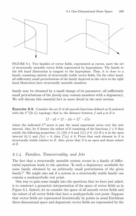
8.1 One-Dimensional State Space 489
FIGURE 8.1. Two families of vector fields, represented as curves, meet the setof structurally unstable vector fields represented by hyperplanes. The family inthe left hand illustration is tangent to the hyperplane. Thus, it is close to afamily consisting entirely of structurally stable vector fields. On the other hand,all sufficiently small perturbations of the family depicted as the curve in the righthand illustration have structurally unstable members.
family may be obtained by a small change of its parameter, all sufficientlysmall perturbations of the family may contain members with a degeneracy.We will discuss this essential fact in more detail in the next section.
Exercise 8.3. Consider the set S of all smooth functions defined on R endowedwith the C1([0, 1]) topology; that is, the distance between f and g in S is
‖f − g‖ = ‖f − g‖0 + ‖f ′ − g′‖0
where the indicated C0-norm is just the usual supremum norm over the unitinterval. Also, let S denote the subset of S consisting of the functions f ∈ S thatsatisfy the following properties: (i) f(0) = 0 and f(1) = 0. (ii) If a is in the openinterval (0, 1) and f(a) = 0, then f ′(a) = 0. Prove that each element in S isstructurally stable relative to S. Also, prove that S is an open and dense subsetof S.
8.1.4 Families, Transversality, and JetsThe fact that a structurally unstable system occurs in a family of differ-ential equations leads to the question “Is such a degeneracy avoidable forsome family obtained by an arbitrarily small perturbation of the givenfamily?” We might also ask if a system in a structurally stable family cancontain a nonhyperbolic rest point.
One way to gain some insight into the questions that we have just asked,is to construct a geometric interpretation of the space of vector fields as inFigure 8.1. Indeed, let us consider the space of all smooth vector fields andthe subset of all vector fields that have a nonhyperbolic rest point. Supposethat vector fields are represented heuristically by points in usual Euclideanthree-dimensional space and degenerate vector fields are represented by the
490 8. Local Bifurcation
points on a hypersurface D. (A three-parameter family of vector fields wouldbe represented by a point in three-dimensional Euclidean space.) Since thecomplement of the set D is dense, if f is a point in D, then there arepoints in the complement of D that are arbitrarily close to f . By analogy,if our geometric interpretation is faithful, then there is an arbitrarily smallC1 perturbation of our vector field f that is nondegenerate; that is, thecorresponding system has only hyperbolic rest points. This is indeed thecase if we restrict our vector fields to compact domains.
Next, consider a one-parameter family of vector fields as a curve in thespace of all smooth vector fields, and suppose that this curve meets thehypersurface D that represents the degenerate vector fields. If the curvemeets the surface so that its tangent vector at the intersection point is nottangent to the surface—we call this a transversal intersection—then everysufficiently small deformation of the curve will have a nonempty transversalintersection with D. In other words, the degeneracy that is encountered byour curve cannot be removed by a perturbation of the curve. By analogy,if our original family of vector fields meets a “surface” corresponding to adegenerate set in the space of all vector fields, and if the intersection of thecurve with this degenerate surface is “transversal,” then the degeneracycannot be removed by a small deformation of the family. This is one of themain reasons why bifurcation theory is important in applied mathematicswhen we are studying a model that is given by a family of differentialequations.
The geometric picture we have discussed gives the correct impressionfor structural instabilities due to the nonhyperbolicity of rest points, thesubject of this chapter. Indeed, we will show how to make a precise in-terpretation of this geometry for scalar vector fields. However, there is animportant warning: Our picture is misleading for some more complicatedstructural instabilities, a topic that is beyond the scope of this book (see,for example, [150] and [160]).
Let us identify the set of all scalar vector fields with the space of smoothfunctions C∞(R, R). In view of Proposition 8.2, only a finite set of thepartial derivatives of a scalar family is required to determine the presenceof a saddle-node bifurcation. In fact, this observation is the starting pointfor the construction of a finite dimensional space, called the space of k-jets,that corresponds to the ambient space in our geometric picture.
The “correct” definition of the space of k-jets requires the introductionof vector bundles (see, for example, [3]). However, we will enjoy a briefglimpse of this theory by considering the special case of the constructionfor the space C∞(R, R) where everything is so simple that the mention ofvector bundles can be avoided.
Consider the space R×C∞(R, R) and let k denote a nonnegative integer.We will say that two elements (x, f) and (y, g) in the cross product space
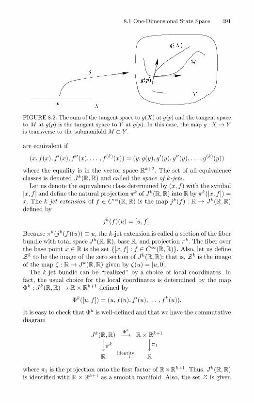
8.1 One-Dimensional State Space 491
Y
pX
g
gp
gX
M
FIGURE 8.2. The sum of the tangent space to g(X) at g(p) and the tangent spaceto M at g(p) is the tangent space to Y at g(p). In this case, the map g : X → Yis transverse to the submanifold M ⊂ Y .
are equivalent if
(x, f(x), f ′(x), f ′′(x), . . . , f (k)(x)) = (y, g(y), g′(y), g′′(y), . . . , g(k)(y))
where the equality is in the vector space Rk+2. The set of all equivalence
classes is denoted Jk(R, R) and called the space of k-jets.Let us denote the equivalence class determined by (x, f) with the symbol
[x, f ] and define the natural projection πk of Jk(R, R) into R by πk([x, f ]) =x. The k-jet extension of f ∈ C∞(R, R) is the map jk(f) : R → Jk(R, R)defined by
jk(f)(u) = [u, f ].
Because πk(jk(f)(u)) ≡ u, the k-jet extension is called a section of the fiberbundle with total space Jk(R, R), base R, and projection πk. The fiber overthe base point x ∈ R is the set [x, f ] : f ∈ C∞(R, R). Also, let us defineZk to be the image of the zero section of Jk(R, R); that is, Zk is the imageof the map ζ : R → Jk(R, R) given by ζ(u) = [u, 0].
The k-jet bundle can be “realized” by a choice of local coordinates. Infact, the usual choice for the local coordinates is determined by the mapΦk : Jk(R, R) → R × R
k+1 defined by
Φk([u, f ]) = (u, f(u), f ′(u), . . . , fk(u)).
It is easy to check that Φk is well-defined and that we have the commutativediagram
Jk(R, R) Φk
−→ R × Rk+1(πk
(π1
Ridentity−→ R
where π1 is the projection onto the first factor of R×Rk+1. Thus, Jk(R, R)
is identified with R × Rk+1 as a smooth manifold. Also, the set Z is given
492 8. Local Bifurcation
in the local coordinates by Z := R × 0. The jet space is the desiredfinite dimensional space that incorporates all the data needed to considerbifurcations that depend only on a finite number of partial derivatives of afamily of scalar vector fields.
We will need the concept of transversality of a map and a submanifold(see Figure 8.2).
Definition 8.4. Suppose that g : X → Y is a smooth map and M denotesa submanifold of the manifold Y . We say that the map g is transverse toM at a point p ∈ X if either g(p) ∈ M , or g(p) ∈ M and the sum of thetangent space of M at g(p) and the range of the derivative Dg(p) (bothviewed as linear subspaces of the tangent space of Y at p) is equal to theentire tangent space of Y at g(p). The function g is said to be transverseto the manifold M if it is transverse to M at every point of X.
The next theorem is stated with some informality. However, it is clearlya far-reaching generalization of the implicit function theorem.
Theorem 8.5 (Thom’s Transversality Theorem). The set S of mapswhose k-jet extensions are transverse to a submanifold M of the space ofk-jets is a dense subset of the space of all sufficiently smooth maps, andmoreover S is a countable intersection of open dense sets. In addition, ifM is closed in the space of k-jets, then S is open.
To make Thom’s theorem precise, we would have to define topologies onour function spaces. The usual Cr topology is induced by the norm definedas the sum of the suprema of the absolute values of the partial derivativesof a function up to order r. However, this topology is not defined on thespace Cr(R, R) because some of the functions in this space are unboundedor have an unbounded partial derivative. To get around this problem, wecan restrict attention to functions defined on a compact domain in R, or wecan use one of the two useful topologies on Cr(R, R) called the weak andthe strong topology. Roughly speaking, if f is a function, α > 0, and K is acompact subset of R, then a basic open set in the weak topology, also calledthe compact open topology, is defined to be the set of functions g such thatthe distance between f and g in the Cr-norm, relative to the compact setK, is less than the positive number α. The strong topology is similar, but itincludes the neighborhoods defined by requiring that functions be close on(infinite) families of compact subsets of their domains. The strong topologyis important because some of its open neighborhoods control the size of thefunction and its partial derivatives “at infinity.” These topologies are thesame if the functions in Cr(R, R) are all restricted to a compact set. Inthis case, the corresponding function space is the usual Banach space of Cr
functions defined on the compact set. However, the important observationfor our discussion is that Thom’s theorem is valid for both the weak andstrong topologies. (See the book of Morris Hirsch [92] for a precise definitionof these topologies and a proof of Thom’s theorem.)
8.1 One-Dimensional State Space 493
A set is called residual if it is the (countable) intersection of open anddense subsets. By Baire’s theorem, every residual set in a complete metricspace is dense (see [156]). Also, a property that holds on a residual set iscalled generic. It turns out that even though the weak and strong topolo-gies on C∞(R, R) are not metrizable, the set C∞(R, R) is a Baire spacewith respect to these topologies; that is, in these topologies a countableintersection of open and dense sets is dense. Using these notions, Thom’stransversality theorem can be restated as follows: The property of transver-sal intersection is generic.
As a simple example of an application of Thom’s theorem, let us considerthe transversality of the 0-jet extensions of functions in C∞(R, R) with theimage of the zero section. Note that by the definition of transversality the 0-jet extension of f ∈ C∞(R, R) is transversal to the image of the zero sectionZ0 at u ∈ R if either j0(f)(u) = [u, 0], or j0(f)(u) = [u, 0] and the imageof the derivative of the 0-jet extension j0(f) at u plus the tangent space toZ0 at [u, 0] is the tangent space to J0(R, R) at [u, 0]. We will determine thistransversality condition more explicitly and use Thom’s theorem to statea fact about the genericity of vector fields with hyperbolic rest points.
The differentiability of the map j0(f) and the properties of its deriva-tive are local properties that can be determined in the local coordinaterepresentation of the jet bundle. In fact, with respect to the local co-ordinates mentioned above, the local representative of the map j0(f) isu → Φ0(j0(f)(u)). In other words, the local representation of j0(f) is themap F : R → R × R defined by u → (u, f(u)); and, in these coordinates,the range of the derivative of F is spanned by the vector (1, f ′(u)).
The local representation of Z0 is given by the linear manifold Z0 :=(x, y) ∈ R × R : y = 0. Hence, the tangent space of Z0 at each of itspoints can be identified with Z0. Moreover, let us note that Z0, viewed asa subspace of R × R, is spanned by the vector (1, 0).
The 0-jet extension of the function f is transverse to the zero section atthe point u ∈ R if and only if f ′(u) = 0; it is transverse to the zero sectionif it is transverse at every u ∈ R. In other words, the 0-jet extension of f istransverse to the zero section if and only if all zeros of f are nondegenerate;or equivalently if and only if all rest points of the corresponding differentialequation u = f(u) are hyperbolic.
By Thom’s theorem, if f is in C∞(R, R), then there is an arbitrarilysmall perturbation of f such that the corresponding differential equationhas only hyperbolic rest points. Moreover, the set of all scalar differentialequations with hyperbolic rest points is open.
The proof of Thom’s theorem is not trivial. However, for the simple casethat we are considering, we can obtain part of Thom’s result as a corollaryof the implicit function theorem. In fact, we will show that if f has finitelymany nondegenerate zeros, then every sufficiently small perturbation of fhas the same property.
494 8. Local Bifurcation
Consider the Banach space C1(R, R) consisting of all elements of C1(R, R)that are bounded in the C1-norm. Suppose that f ∈ C1(R, R) has onlynondegenerate zeros and consider the map ρ : R × C1(R, R) → R given by(u, f) → f(u). This map is smooth. Moreover, if ρ(u0, f0) = 0, then wehave ρu(u0, f0) = f ′(u0) = 0. Thus, there is a map f → β(f) defined on aneighborhood U of f0 in C1(R, R) with image in an open subset V ⊂ R suchthat β(f0) = u0 and f(β(f)) ≡ 0. Moreover, if (u, f) ∈ V ×U and f(u) = 0,then u = β(f). In other words, every function in the neighborhood U hasexactly one zero in V . Also, there are open subsets U0 ⊆ U and V0 ⊆ Vsuch that for each function f in U0 we have f ′(u) = 0 whenever u ∈ V0.Hence, every function in U0 has a unique nondegenerate zero in V0. If, inaddition, the function f has only finitely many zeros, then we can be surethat every perturbation of f has only nondegenerate zeros.
Exercise 8.6. Consider the set of differential equations of the form u = f(u),where u ∈ R
n, that have a finite number of rest points, and show that the subsetof these systems with hyperbolic rest points is open and dense in the C1 topology.
We have used jet spaces to analyze the perturbations of scalar differentialequations that have only hyperbolic rest points. We will discuss differentialequations with saddle-nodes and show that the conditions required for asaddle-node are the same as the conditions for a certain jet extension mapto be transversal to the zero section of a jet bundle.
Consider the 1-jet extensions of smooth scalar maps and the image ofthe zero section Z1 ⊂ J1(R, R). If j1(f)(u) ∈ Z1, then f has a saddle-nodeat u; that is, f(u) = 0 and f ′(u) = 0. However, to study the saddle-nodebifurcation, we must consider families of maps in C∞(R, R). In fact, wewill identify these families as elements of the space C∞(R × R, R) where atypical element f is given by a function of two variables (u, ε) → f(u, ε).
Let us define a new jet bundle with total space J (1,0)(R×R, R) consistingof all equivalence classes of triples (u, ε, f) ∈ R × R × C∞(R × R, R) wherethe triples (v, δ, f) and (w, ν, g) are equivalent if
v = w, δ = ν, f(v, δ) = g(w, ν), fu(v, δ) = gu(w, ν),
and the bundle projection is given by [u, ε, f(u, ε), fu(u, ε)] → (u, ε). Oursomewhat nonstandard jet space J (1,0)(R×R, R) may be viewed as a spaceof families of sections of the 1-jet bundle of functions in C∞(R, R).
The (1, 0)-jet extension of f ∈ C∞(R × R, R) is the map
j(1,0)(f) : R × R → J (1,0)(R × R, R)
given by j(1,0)(f)(u, ε) = [u, ε, f(u, ε), fu(u, ε)], and the image of the zerosection Z(1,0) is the set of all equivalence classes of triples of the form(u, ε, 0).
8.1 One-Dimensional State Space 495
Let us note that the local representative of the (1, 0)-jet extension isgiven by
(u, ε) → (u, ε, f(u, ε), fu(u, ε)).
Note also that the (1, 0)-jet extension is transverse to the zero section Z(1,0)
at a point (u, ε) where f(u, ε) = 0 and fu(u, ε) = 0 if the following obtains:The vector space sum of(i) the range of the derivative of the local representative of the (1, 0)-jet
extension; and(ii) the tangent space of the local representation of Z(1,0) at (u, ε, 0, 0)
is equal to the entire space R4. By (i) and (ii) we mean
(i) the span of the vectors
(1, 0, fu(u, ε), fuu(u, ε)) and (0, 1, fε(u, ε), fεu(u, ε)); and
(ii) the span of the vectors (1, 0, 0, 0) and (0, 1, 0, 0).This transversality condition is met provided that
fε(u, ε) = 0 and fεu(u, ε) = 0,
exactly the conditions for a nondegenerate saddle-node bifurcation!Just as for the case of nondegenerate zeros, the subset of all families of
smooth maps that have a saddle-node bifurcation is dense, and this set canbe identified as the countable intersection of open and dense subsets of thespace C∞(R×R, R). Moreover, by using the implicit function theorem, it iseasy to prove that if a family has a saddle-node bifurcation at some point,then a small perturbation of this family also has a saddle-node bifurcationat a nearby point. Thus, we have a rigorous argument that the saddle-node bifurcation can be unavoidable in all families obtained as the resultof sufficiently small perturbations of some one-parameter family of maps;and, as a result, we have a positive answer to the question “Is bifurcationtheory important?”
Exercise 8.7. Formulate and prove a theorem based on the implicit functiontheorem that can be used to show that a small perturbation of a family of mapswith a saddle-node bifurcation has a nearby saddle-node bifurcation.
We have discussed the unavoidability of the saddle-node bifurcation inone-parameter families of maps. This leads to the question “Are saddle-nodes unavoidable in two-parameter families of maps?” The answer is“yes.” In fact, nothing new happens for the saddle-node bifurcation relativeto multiparameter families of maps. The reason is that the set correspond-ing to the saddle-node has codimension one in an appropriate functionspace.
496 8. Local Bifurcation
In the remainder of this chapter we will not pursue the ideas that we havediscussed in this section. Rather, we will only consider sufficient conditionsto obtain nondegenerate bifurcation in one-parameter families. However,transversality theory can be applied in each case that we will consider toshow that, in an appropriate sense, the bifurcations are generic.
Finally, bifurcation theory in families with two or more parameters isgenerally much more difficult than the theory for one-parameter families.For example, the analysis of generic bifurcations at a degenerate rest pointin two-parameter families requires that global features of the dynamics betaken into account (see, for example, [49], [50], [80], and [185]).
Exercise 8.8. Prove: The map R × C1([a, b], R) → R given by (u, f) → f(u) issmooth.
Exercise 8.9. Prove: There is a saddle-node bifurcation for some values of theparameter ε in the family
u = cos ε − u sin u.
Exercise 8.10. Draw the bifurcation diagram for the scalar family of differen-tial equations
x = εx − x2.
The bifurcation at ε = 0 is called transcritical. Prove a proposition similar toProposition 8.2 for the existence of a transcritical bifurcation.
Exercise 8.11. Draw the bifurcation diagram for the scalar family of differen-tial equations
x = εx − x3.
The bifurcation at ε = 0 is called the pitchfork. Prove a proposition similar toProposition 8.2 for the existence of a pitchfork bifurcation.
8.2 Saddle-Node Bifurcation byLyapunov–Schmidt Reduction
In this section we will consider the saddle-node bifurcation for the n-dimensional system (8.1). It should be clear from the previous discus-sion that the conditions for the saddle-node bifurcation do not mentionthe solutions of the differential equations in this family, rather our anal-ysis so far is framed entirely in terms of a parameter-dependent functionf : R
n × R → Rn that defines the vector field associated with our family of
differential equations. In view of this fact, we say that u0 ∈ Rn is a saddle-
node for f : Rn × R → R
n at ε0 if f(u0, ε0) = 0, the linear transformationfu(u0, ε0) : R
n → Rn has zero as an eigenvalue with algebraic multiplicity
8.2 Saddle-Node Bifurcation by Lyapunov–Schmidt Reduction 497
one, and all other eigenvalues have nonzero real parts. Also, a saddle-nodebifurcation is said to occur at a saddle-node u = u0 for the parameter valueε = ε0 if the following conditions are met:
SNB1 There is a number p0 > 0 and a smooth curve p → β(p) in Rn ×R
such that β(0) = (u0, ε0) and f(β(p)) ≡ 0 for |p| < p0.SNB2 The curve β has a quadratic tangency with R
n × ε0 at (u0, ε0).More precisely, if the components of β are defined by
β(p) = (β1(p), β2(p)),
then β2(0) = ε0, β′2(0) = 0, and β′′
2 (0) = 0.SNB3 If p = 0, then the matrix fu(β(p)) is infinitesimally hyperbolic.
Also, exactly one eigenvalue of the matrix crosses the imaginaryaxis with nonzero speed at the parameter value p = 0.
The next theorem, called the saddle-node bifurcation theorem, gives suf-ficient generic conditions for a saddle-node bifurcation to occur.
Theorem 8.12. Suppose that f : Rn × R → R
n is a smooth function,u = u0 is a saddle-node for f at ε = ε0, and the kernel of the lineartransformation fu(u0, ε0) : R
n → Rn is spanned by the nonzero vector
k ∈ Rn. If fε(u0, ε0) ∈ R
n and fuu(u0, ε0)(k, k) ∈ Rn are both nonzero and
both not in the range of fu(u0, ε0), then there is a saddle-node bifurcationat u = u0 (that is SNB1, SNB2, and SNB3 are met). Moreover, among allC∞ one-parameter families that have a saddle-node, those that undergo asaddle-node bifurcation form an open and dense subset.
The second derivatives that appear in the statement of Theorem 8.12are easily understood from the correct point of view. Indeed, suppose thatg : R
n → Rn is a smooth function given by u → g(u) and recall that its
(first) derivative Dg is a map from Rn into the linear transformations of R
n;that is, Dg : R
n → L(Rn, Rn). If u, v, w ∈ Rn, then the derivative of g at u
in the direction w is denoted by Dg(u)w. Consider the map u → Dg(u)w.If g ∈ C2, then its derivative at u ∈ R
n in the direction v is defined by
d
dtDg(u + tv)w
∣∣∣t=0
= (D2g(u)w)v = D2g(u)(w, v).
Hence, if g ∈ C2, then to compute the second derivative D2g, it suffices tocompute the first derivative of the map u → Dg(u)w.
Exercise 8.13. Define g : R × R → R by
g(x, y, ε) = (ε − x2 + xy, −2y + x2 + y2)
and u := (x, y). Compute guu(0, 0, 0)(e1, e1) where e1 = (1, 0).
498 8. Local Bifurcation
Exercise 8.14. Prove that if g ∈ C2, then D2g(u)(v, w) = D2g(u)(w, v).
We now turn to the proof of Theorem 8.12.
Proof. Assume, with no loss of generality, that u = 0 is a saddle-nodefor f at ε = 0. Also, assume that zero is an eigenvalue of the linearizationfu(0, 0) : R
n → Rn with algebraic multiplicity one, and the kernel K of this
linear transformation is one-dimensional, say K = [k].Using the Lyapunov–Schmidt reduction and linear algebra, let us choose
an (n − 1)-dimensional complement K⊥ to K in Rn whose basis is
k⊥2 , . . . , k⊥
n .
Corresponding to these choices, there is a coordinate transformation Ψ :R × R
n−1 → Rn given by
(p, q) → pk +n∑
i=2
qik⊥i
where, in the usual coordinates of Rn−1, the point q is given by q =
(q2, . . . , qn). Likewise, the range R of fu(0, 0) is (n − 1)-dimensional witha one-dimensional complement R⊥. Let Π : R
n → R and Π⊥ : Rn → R⊥
be corresponding complementary linear projections.With the notation defined above, consider the map : R × R
n−1 ×R → R given by (p, q, ε) → Πf(Ψ(p, q), ε). Since f(0, 0) = 0, we havethat (0, 0, 0) = 0. From equation (5.60) of the abstract formulation of theLyapunov–Schmidt reduction, we see that q(0, 0, 0) is invertible as a lineartransformation R
n−1 → Rn−1. Thus, there is a function h : R × R → R
n−1
given by (p, ε) → h(p, ε) with h(0, 0) = 0 such that for (p, ε) in a sufficientlysmall neighborhood of the origin in R
n−1 × R we have
Πf(Ψ(p, h(p, ε), ε)) ≡ 0. (8.6)
It is instructive to check the invertibility of the derivative directly. Infact, we have
q(0, 0, 0) = Πfu(0, 0)Ψq(0, 0).
But Ψq(0, 0) : Rn−1 → R
n is given by
Ψq(0, 0)q =n∑
i=2
qik⊥i .
Hence, the range of Ψq is the complement of the Kernel fu(0, 0) previouslychosen. Also Ψq is an isomorphism onto its range. On the complement ofits kernel, fu(0, 0) is an isomorphism onto its range and Π is the identityon this range. In other words, q(0, 0, 0) is an isomorphism.
8.2 Saddle-Node Bifurcation by Lyapunov–Schmidt Reduction 499
Viewed geometrically, the function h defines a two-dimensional surfacein R × R
n−1 × R given by (p, h(p, ε), ε) : (p, ε) ∈ Rn × R which lies in
the zero set of . In addition, the (Lyapunov–Schmidt) reduced function isτ : R × R → R⊥ defined by
(p, ε) → Π⊥f(Ψ(p, h(p, ε)), ε).
Of course, if (p, ε) is a zero of τ , then f(Ψ(p, h(p, ε)), ε) = 0.We have τ(0, 0) = 0. If τε(0, 0) = 0, then by the implicit function theorem
there is a unique curve p → γ(p) in R such that γ(0) = 0 and τ(p, γ(p)) ≡ 0.Moreover, in this case, it follows that
f(Ψ(p, h(p, γ(p))), γ(p)) ≡ 0.
In other words, the image of the function β defined by
p → (Ψ(p, h(p, γ(p)), γ(p))
is a curve in the zero set of f(u, ε) that passes through the point (u, ε) =(0, 0).
To show SNB1, we will prove that τε(0, 0) = 0. Let us note first that
τε(0, 0) = Π⊥(fu(0, 0)Ψq(0, 0)hε(0, 0) + fε(0, 0)).
Since Π⊥ projects to the complement of the range of fu(0, 0), the lastformula reduces to
τε(0, 0) = Π⊥fε(0, 0).
But by hypothesis, fε(0, 0) ∈ R and τε(0, 0) = 0, as required.To prove SNB2, we will show that γ′(0) = 0 and γ′′(0) = 0. Note first
that the derivative of the identity τ(p, γ(p)) ≡ 0 with respect to p is givenby
τp(p, γ(p)) + τε(p, γ(p))γ′(p) ≡ 0. (8.7)
Moreover, if we set p = 0 and use the equality γ(0) = 0, then
τp(0, 0) + τε(0, 0)γ′(0) = 0.
Next, recall that τε(0, 0) = 0. Also, use the definition of τ to compute
τp(p, ε) = Π⊥fu(Ψ(p, h(p, ε)), ε)(Ψp(p, h(p, ε)) + Ψq(p, h(p, ε))hp(p, ε)
),
(8.8)
and, in particular,
τp(0, 0) = Π⊥fu(0, 0)(Ψp(0, 0) + Ψq(0, 0)hp(0, 0)
).
500 8. Local Bifurcation
Because Π⊥ projects to the complement of the range of fu(0, 0), it followsthat τp(0, 0) = 0, and therefore γ′(0) = 0. Also, from equation (8.7) andthe fact that γ′(0) = 0, we obtain the equality
τpp(0, 0) + τε(0, 0)γ′′(0) = 0.
Thus, it follows that
γ′′(0) = −τpp(0, 0)τε(0, 0)
.
To prove the inequality τpp(0, 0) = 0, first use equation (8.8) and the factthat Π⊥ projects to the complement of the range of fu(0, 0) to obtain theequality
τpp(0, 0) = Π⊥fuu(0, 0)(Ψp(0, 0) + Ψq(0, 0)hp(0, 0)
)2
where “the square” is shorthand for the argument of the bilinear formfuu(0, 0) on R
n.Next, differentiate the identity (8.6) with respect to p at p = 0 to obtain
the equation
Πfu(0, 0)(Ψp(0, 0) + Ψq(0, 0)hp(0, 0)
)= 0. (8.9)
Then using the fact that Π projects to the range of fu(0, 0) we see thatequation (8.9) is equivalent to the equation
fu(0, 0)(Ψp(0, 0) + Ψq(0, 0)hp(0, 0)) = 0,
and therefore the vector
Ψp(0, 0) + Ψq(0, 0)hp(0, 0)
is in the kernel K of fu(0, 0). But by the definition of Ψ we have Ψp(0, 0) =k ∈ K and Ψq(0, 0)hp(0, 0) ∈ K⊥. Thus, hp(0, 0) = 0, and it follows thatτpp(0, 0) = 0 if and only if
fuu(0, 0)(k, k) = 0, fuu(0, 0)(k, k) ∈ R. (8.10)
This completes the proof of SNB2.To prove SNB3, and thus complete the proof of the theorem, let us
consider the curve β of rest points given by p → (Ψ(p, h(p, γ(p)), γ(p)). Wemust show that the matrix fu(β(p)) is invertible for small nonzero p ∈ R
and a single eigenvalue of fu(β(p)) passes through zero with nonzero speedat p = 0. In other words, the rest points on the curve β are hyperbolic forp = 0, and there is a generic change of stability at p = 0. Of course, thefirst condition follows from the second.
To analyze the second condition, let us consider the eigenvalues of thelinearization f(β(p)). By the hypothesis of the theorem, there is exactly one
8.2 Saddle-Node Bifurcation by Lyapunov–Schmidt Reduction 501
zero eigenvalue at p = 0. Thus, there is a curve p → λ(p) in the complexplane such that λ(0) = 0 and such that λ(p) is an eigenvalue of f(β(p)).Also, there is a corresponding eigenvector V (p) such that
fu(β(p))V (p) = λ(p)V (p), (8.11)V (0) = k.
If the identity (8.11) is differentiated with respect to p at p = 0, then, aftersome simplification, we obtain the equation
fuu(0, 0)(k, k) + fu(0, 0)V ′(0) = λ′(0)k,
and its projectionΠ⊥fuu(k, k) = λ′(0)Π⊥k.
By the inequality (8.10), we have that Π⊥fuu(0, 0)(k, k) = 0, and thereforeλ′(0) is a nonzero real number.
Exercise 8.15. Prove: With the notation as in the proof of Theorem 8.12, ifΠ⊥k = 0 and n ≥ 2, then zero is an eigenvalue of fu(0, 0) with multiplicity atleast two.
Exercise 8.16. Suppose that A : Rn → R
n is a linear transformation withexactly one zero eigenvalue. Show that there is a nonzero “left eigenvector” w ∈R
n such that wTA = 0. Also, show that v is in the range of A if and only if〈v, w〉 = 0. Discuss how this exercise gives a method to verify the hypotheses ofTheorem 8.12.
Exercise 8.17. Verify the existence of a saddle-node bifurcation for the func-tion f : R
2 × R → R2 given by
f(x, y, ε) = (ε − x2, −y).
Exercise 8.18. Determine the bifurcation diagram for the phase portrait ofthe differential equation
xx + ax2 = b
where a and b are parameters.
Exercise 8.19. [Hamiltonian saddle-node] Suppose that
u = f(u, λ), u ∈ R2 (8.12)
is a planar Hamiltonian family with parameter λ ∈ R. Prove that if f(u0, λ0) = 0and the corresponding linearization at u0 has a zero eigenvalue, then this eigen-value has algebraic multiplicity two. In particular, a planar Hamiltonian systemcannot have a saddle-node. Define (u0, λ0) to be a Hamiltonian saddle-node atλ0 if f(u0, λ0) = 0 and fu(u0, λ0) has a zero eigenvalue with geometric multiplic-ity one. A Hamiltonian saddle-node bifurcation occurs if the following conditionshold:
502 8. Local Bifurcation
• There exist s0 > 0 and a smooth curve γ in R2×R such that γ(0) = (u0, λ0)and f(γ(s)) ≡ 0 for |s| < s0.
• The curve of critical points γ is quadratically tangent to R2 × λ0 at(u0, λ0).
• The Lyapunov stability type of the rest points on the curve γ changes ats = 0.
Prove the following proposition formulated by Jason Bender [20]: Suppose thatthe origin in R
2 × R is a Hamiltonian saddle-node for (8.12) and k ∈ R2 is anonzero vector that spans the one-dimensional kernel of the linear transformationfu(0, 0). If the two vectors fλ(0, 0) ∈ R2 and fuu(0, 0)(k, k) ∈ R2 are nonzero andnot in the range of fu(0, 0), then a Hamiltonian saddle-node bifurcation occursat the origin.
Reformulate the hypotheses of the proposition in terms of the Hamiltonianfor the family so that there is no mention of the vector k. Also, discuss theHamiltonian saddle-node bifurcation for the following model of a pendulum withfeedback control
x = y, y = − sin x − αx + β
(see [188]). Generalize the proposition to Hamiltonian systems on R2n. (See [123]
for the corresponding result for Poincare maps at periodic orbits of Hamiltoniansystems.)
8.3 Poincare–Andronov–Hopf Bifurcation
Consider the family of differential equations
u = F (u, λ), u ∈ RN , λ ∈ R
M (8.13)
where λ is a vector of parameters.
Definition 8.20. An ordered pair (u0, λ0) ∈ RN × R
M consisting of aparameter value λ0 and a rest point u0 for the corresponding member ofthe family (8.13) is called a Hopf point if there is a curve C in R
N × RM ,
called an associated curve, that is given by ε → (C1(ε), C2(ε)) and satisfiesthe following properties:
(i) C(0) = (u0, λ0) and F (C1(ε), C2(ε)) ≡ 0.
(ii) The linear transformation given by the derivative Fu(C1(ε), C2(ε)) :R
N → RN has a pair of nonzero complex conjugate eigenvalues α(ε)±
β(ε) i, each with algebraic (and geometric) multiplicity one. Also,α(0) = 0, α′(0) = 0, and β(0) = 0.
(iii) Except for the eigenvalues ±β(0) i, all other eigenvalues of Fu(u0, λ0)have nonzero real parts.
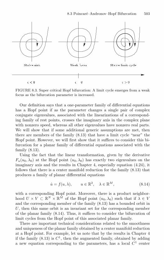
8.3 Poincare–Andronov–Hopf Bifurcation 503
Stable limit cycle
Stable sink Weak focus
FIGURE 8.3. Super critical Hopf bifurcation: A limit cycle emerges from a weakfocus as the bifurcation parameter is increased.
Our definition says that a one-parameter family of differential equationshas a Hopf point if as the parameter changes a single pair of complexconjugate eigenvalues, associated with the linearizations of a correspond-ing family of rest points, crosses the imaginary axis in the complex planewith nonzero speed, whereas all other eigenvalues have nonzero real parts.We will show that if some additional generic assumptions are met, thenthere are members of the family (8.13) that have a limit cycle “near” theHopf point. However, we will first show that it suffices to consider this bi-furcation for a planar family of differential equations associated with thefamily (8.13).
Using the fact that the linear transformation, given by the derivativeFu(u0, λ0) at the Hopf point (u0, λ0) has exactly two eigenvalues on theimaginary axis and the results in Chapter 4, especially equation (4.24), itfollows that there is a center manifold reduction for the family (8.13) thatproduces a family of planar differential equations
u = f(u, λ), u ∈ R2, λ ∈ R
M , (8.14)
with a corresponding Hopf point. Moreover, there is a product neighbor-hood U × V ⊂ R
N × RM of the Hopf point (u0, λ0) such that if λ ∈ V
and the corresponding member of the family (8.13) has a bounded orbit inU , then this same orbit is an invariant set for the corresponding memberof the planar family (8.14). Thus, it suffices to consider the bifurcation oflimit cycles from the Hopf point of this associated planar family.
There are important technical considerations related to the smoothnessand uniqueness of the planar family obtained by a center manifold reductionat a Hopf point. For example, let us note that by the results in Chapter 4if the family (8.13) is C1, then the augmented family, obtained by addinga new equation corresponding to the parameters, has a local C1 center
504 8. Local Bifurcation
manifold. But this result is not strong enough for the proof of the Hopfbifurcation theorem given below. In fact, we will require the reduced planarsystem (8.14) to be C4. Fortunately, the required smoothness can be proved.In fact, using the fiber contraction principle as in Chapter 4, together withan induction argument, it is possible to prove that if 0 < r < ∞ and thefamily (8.13) is Cr, then the reduced planar system at the Hopf point is alsoCr in a neighborhood of the Hopf point. Let us also note that whereas localcenter manifolds are not necessarily unique, it turns out that all rest points,periodic orbits, homoclinic orbits, et cetera, that are sufficiently close tothe original rest point, are on every center manifold. Thus, the bifurcationphenomena that are determined by reduction to a center manifold do notdepend on the choice of the local center manifold (see, for example, [50]).
Let us say that a set S has radius (r1, r2) relative to a point p if S iscontained in a ball of radius r1 > 0 centered at p and the distance from Sto p is r2 ≥ 0.
Definition 8.21. The planar family (8.14) has a supercritical Hopf bifur-cation at a Hopf point with associated curve ε → (c1(ε), c2(ε)) if there arethree positive numbers ε0, K1, and K2 such that for each ε in the openinterval (0, ε0) the differential equation u = f(u, c2(ε)) has a hyperboliclimit cycle with radius
(K1√
ε + O(ε), K2√
ε + O(ε))
relative to the rest point u = c1(ε). If there is a similar limit cycle forthe systems with parameter values in the range −ε0 < ε < 0, then thebifurcation is called subcritical. Also, we say that the family (8.13) has asupercritical (respectively, subcritical) Hopf bifurcation at a Hopf point ifthe corresponding (center manifold) reduced system (8.14) has a supercrit-ical (respectively, subcritical) Hopf bifurcation.
To avoid mentioning several similar cases as we proceed, let us consideronly Hopf points such that the parametrized eigenvalues α±β i satisfy theadditional assumptions
α′(0) > 0, β(0) > 0. (8.15)
In particular, we will restrict attention to the supercritical Hopf bifurcationas depicted in Figure 8.3.
Under our standing hypothesis (8.15), a rest point on the associated curveε → c(ε) of the Hopf point is a stable hyperbolic focus for the correspondingsystem (8.14) for ε < 0 and an unstable hyperbolic focus for ε > 0. We willintroduce an additional hypothesis that implies “weak attraction” towardthe rest point u0 at the parameter value λ0. In this case, there is a stablelimit cycle that “bifurcates from this rest point” as ε increases through ε =0. This change in the qualitative behavior of the system as the parameter
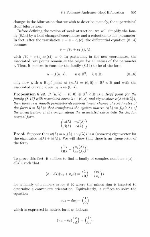
8.3 Poincare–Andronov–Hopf Bifurcation 505
changes is the bifurcation that we wish to describe, namely, the supercriticalHopf bifurcation.
Before defining the notion of weak attraction, we will simplify the fam-ily (8.14) by a local change of coordinates and a reduction to one-parameter.In fact, after the translation v = u − c1(ε), the differential equation (8.14)becomes
v = f(v + c1(ε), λ)
with f(0 + c1(ε), c2(ε)) ≡ 0. In particular, in the new coordinates, theassociated rest points remain at the origin for all values of the parameterε. Thus, it suffices to consider the family (8.14) to be of the form
u = f(u, λ), u ∈ R2, λ ∈ R, (8.16)
only now with a Hopf point at (u, λ) = (0, 0) ∈ R2 × R and with the
associated curve c given by λ → (0, λ).
Proposition 8.22. If (u, λ) = (0, 0) ∈ R2 × R is a Hopf point for the
family (8.16) with associated curve λ → (0, λ) and eigenvalues α(λ)±β(λ) i,then there is a smooth parameter-dependent linear change of coordinates ofthe form u = L(λ)z that transforms the system matrix A(λ) := fu(0, λ) ofthe linearization at the origin along the associated curve into the Jordannormal form (
α(λ) −β(λ)β(λ) α(λ)
).
Proof. Suppose that w(λ) = u1(λ) + u2(λ) i is a (nonzero) eigenvector forthe eigenvalue α(λ) + β(λ) i. We will show that there is an eigenvector ofthe form (1
0
)−
(v1(λ)v2(λ)
)i.
To prove this fact, it suffices to find a family of complex numbers c(λ) +d(λ) i such that
(c + d i)(u1 + u2 i) =(1
0
)−
(v1v2
)i
for a family of numbers v1, v2 ∈ R where the minus sign is inserted todetermine a convenient orientation. Equivalently, it suffices to solve theequation
cu1 − du2 =(1
0
)which is expressed in matrix form as follows:
(u1,−u2)(
cd
)=
(10
).
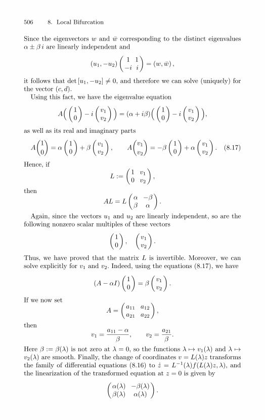
506 8. Local Bifurcation
Since the eigenvectors w and w corresponding to the distinct eigenvaluesα ± β i are linearly independent and
(u1,−u2)(
1 1−i i
)= (w, w) ,
it follows that det [u1,−u2] = 0, and therefore we can solve (uniquely) forthe vector (c, d).
Using this fact, we have the eigenvalue equation
A((
10
)− i
(v1v2
))= (α + iβ)
((10
)− i
(v1v2
)),
as well as its real and imaginary parts
A
(10
)= α
(10
)+ β
(v1v2
), A
(v1
v2
)= −β
(10
)+ α
(v1v2
). (8.17)
Hence, if
L :=(
1 v10 v2
),
then
AL = L
(α −ββ α
).
Again, since the vectors u1 and u2 are linearly independent, so are thefollowing nonzero scalar multiples of these vectors(
10
),
(v1v2
).
Thus, we have proved that the matrix L is invertible. Moreover, we cansolve explicitly for v1 and v2. Indeed, using the equations (8.17), we have
(A − αI)(
10
)= β
(v1v2
).
If we now set
A =(
a11 a12a21 a22
),
thenv1 =
a11 − α
β, v2 =
a21
β.
Here β := β(λ) is not zero at λ = 0, so the functions λ → v1(λ) and λ →v2(λ) are smooth. Finally, the change of coordinates v = L(λ)z transformsthe family of differential equations (8.16) to z = L−1(λ)f(L(λ)z, λ), andthe linearization of the transformed equation at z = 0 is given by(
α(λ) −β(λ)β(λ) α(λ)
).
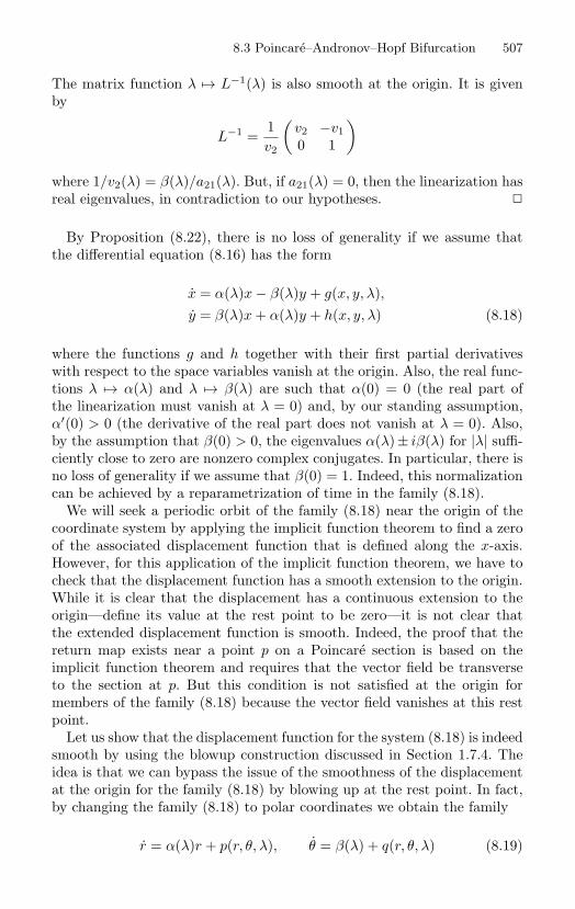
8.3 Poincare–Andronov–Hopf Bifurcation 507
The matrix function λ → L−1(λ) is also smooth at the origin. It is givenby
L−1 =1v2
(v2 −v10 1
)where 1/v2(λ) = β(λ)/a21(λ). But, if a21(λ) = 0, then the linearization hasreal eigenvalues, in contradiction to our hypotheses.
By Proposition (8.22), there is no loss of generality if we assume thatthe differential equation (8.16) has the form
x = α(λ)x − β(λ)y + g(x, y, λ),y = β(λ)x + α(λ)y + h(x, y, λ) (8.18)
where the functions g and h together with their first partial derivativeswith respect to the space variables vanish at the origin. Also, the real func-tions λ → α(λ) and λ → β(λ) are such that α(0) = 0 (the real part ofthe linearization must vanish at λ = 0) and, by our standing assumption,α′(0) > 0 (the derivative of the real part does not vanish at λ = 0). Also,by the assumption that β(0) > 0, the eigenvalues α(λ)± iβ(λ) for |λ| suffi-ciently close to zero are nonzero complex conjugates. In particular, there isno loss of generality if we assume that β(0) = 1. Indeed, this normalizationcan be achieved by a reparametrization of time in the family (8.18).
We will seek a periodic orbit of the family (8.18) near the origin of thecoordinate system by applying the implicit function theorem to find a zeroof the associated displacement function that is defined along the x-axis.However, for this application of the implicit function theorem, we have tocheck that the displacement function has a smooth extension to the origin.While it is clear that the displacement has a continuous extension to theorigin—define its value at the rest point to be zero—it is not clear thatthe extended displacement function is smooth. Indeed, the proof that thereturn map exists near a point p on a Poincare section is based on theimplicit function theorem and requires that the vector field be transverseto the section at p. But this condition is not satisfied at the origin formembers of the family (8.18) because the vector field vanishes at this restpoint.
Let us show that the displacement function for the system (8.18) is indeedsmooth by using the blowup construction discussed in Section 1.7.4. Theidea is that we can bypass the issue of the smoothness of the displacementat the origin for the family (8.18) by blowing up at the rest point. In fact,by changing the family (8.18) to polar coordinates we obtain the family
r = α(λ)r + p(r, θ, λ), θ = β(λ) + q(r, θ, λ) (8.19)
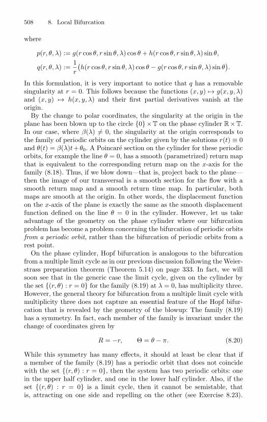
508 8. Local Bifurcation
where
p(r, θ, λ) := g(r cos θ, r sin θ, λ) cos θ + h(r cos θ, r sin θ, λ) sin θ,
q(r, θ, λ) :=1r
(h(r cos θ, r sin θ, λ) cos θ − g(r cos θ, r sin θ, λ) sin θ
).
In this formulation, it is very important to notice that q has a removablesingularity at r = 0. This follows because the functions (x, y) → g(x, y, λ)and (x, y) → h(x, y, λ) and their first partial derivatives vanish at theorigin.
By the change to polar coordinates, the singularity at the origin in theplane has been blown up to the circle 0× T on the phase cylinder R × T.In our case, where β(λ) = 0, the singularity at the origin corresponds tothe family of periodic orbits on the cylinder given by the solutions r(t) ≡ 0and θ(t) = β(λ)t+θ0. A Poincare section on the cylinder for these periodicorbits, for example the line θ = 0, has a smooth (parametrized) return mapthat is equivalent to the corresponding return map on the x-axis for thefamily (8.18). Thus, if we blow down—that is, project back to the plane—then the image of our transversal is a smooth section for the flow with asmooth return map and a smooth return time map. In particular, bothmaps are smooth at the origin. In other words, the displacement functionon the x-axis of the plane is exactly the same as the smooth displacementfunction defined on the line θ = 0 in the cylinder. However, let us takeadvantage of the geometry on the phase cylinder where our bifurcationproblem has become a problem concerning the bifurcation of periodic orbitsfrom a periodic orbit, rather than the bifurcation of periodic orbits from arest point.
On the phase cylinder, Hopf bifurcation is analogous to the bifurcationfrom a multiple limit cycle as in our previous discussion following the Weier-strass preparation theorem (Theorem 5.14) on page 333. In fact, we willsoon see that in the generic case the limit cycle, given on the cylinder bythe set (r, θ) : r = 0 for the family (8.19) at λ = 0, has multiplicity three.However, the general theory for bifurcation from a multiple limit cycle withmultiplicity three does not capture an essential feature of the Hopf bifur-cation that is revealed by the geometry of the blowup: The family (8.19)has a symmetry. In fact, each member of the family is invariant under thechange of coordinates given by
R = −r, Θ = θ − π. (8.20)
While this symmetry has many effects, it should at least be clear that ifa member of the family (8.19) has a periodic orbit that does not coincidewith the set (r, θ) : r = 0, then the system has two periodic orbits: onein the upper half cylinder, and one in the lower half cylinder. Also, if theset (r, θ) : r = 0 is a limit cycle, then it cannot be semistable, thatis, attracting on one side and repelling on the other (see Exercise 8.23).
8.3 Poincare–Andronov–Hopf Bifurcation 509
The Hopf bifurcation theory for this case serves as a simple example of abifurcation with symmetry—an important topic that is covered in detail inthe excellent books [74] and [75].
Exercise 8.23. Prove: If the set Γ := (r, θ) : r = 0 on the cylinder is a limitcycle for the member of the family (8.19) at λ = 0, then this limit cycle is notsemistable. State conditions that imply Γ is a limit cycle and conditions thatimply it is a hyperbolic limit cycle.
By our hypotheses, if |r| is sufficiently small, then the line (r, θ) : θ = 0is a transversal to the flow of system (8.19) on the phase cylinder. More-over, as we have mentioned above, there is a smooth displacement functiondefined on this transversal. In fact, let t → (r(t, ξ, λ), θ(t, ξ, λ)) denote thesolution of the differential equation (8.19) with the initial condition
r(0, ξ, λ) = ξ, θ(0, ξ, λ) = 0,
and note that
θ(2π, 0, 0) = 2π, θ(2π, 0, 0) = β(0) = 0.
By an application of the implicit function theorem, there is a product neigh-borhood U0×V0 of the origin in R×R, and a function T : U0×V0 → R suchthat T (0, 0) = 2π and θ(T (ξ, λ), ξ, λ) ≡ 2π. Thus, the desired displacementfunction δ : U0 × V0 → R is defined by
δ(ξ, λ) := r(T (ξ, λ), ξ, λ) − ξ. (8.21)
The displacement function (8.21) can be difficult to work with because ofthe presence of the implicitly defined return time function T . However, wewill see that problem can be avoided by yet another change of coordinates.Indeed, since T (0, 0) = 2π and θ(t, ξ, 0) = β(0) = 0, it follows from thecontinuity of the functions T and θ that there is a product neighborhoodU ×V of the origin with U ×V ⊆ U0 ×V0 such that for each (ξ, λ) ∈ U ×Vthe function t → θ(t, ξ, λ) is invertible on some bounded time intervalcontaining T (ξ, λ). Moreover, if the inverse function is denoted by s →θ−1(s, ξ, λ), then the function ρ : R × U × V → R defined by
ρ(s, ξ, λ) = r(θ−1(s, ξ, λ), ξ, λ)
is a solution of the initial value problem
dρ
ds=
α(λ)ρ + p(ρ, s, λ)β(λ) + q(ρ, s, λ)
, ρ(0, ξ, λ) = ξ
and
ρ(2π, ξ, λ) = r(T (ξ, λ), ξ, λ).
510 8. Local Bifurcation
If we rename the variables ρ and s to new variables r and θ, then thedisplacement function δ : U × V → R as defined in equation (8.21) withrespect to the original variable r is also given by the formula
δ(ξ, λ) = r(2π, ξ, λ) − ξ (8.22)
where θ → r(θ, ξ, λ) is the solution of the initial value problem
dr
dθ=
α(λ)r + p(r, θ, λ)β(λ) + q(r, θ, λ)
, r(0, ξ, λ) = ξ. (8.23)
In particular, with respect to the differential equation (8.23), the “returntime” does not depend on the position ξ along the Poincare section or thevalue of the parameter λ; rather, it has the constant value 2π.
Definition 8.24. Suppose that (u, λ) = (0, 0) ∈ R2 × R is a Hopf point
for the family (8.16). The corresponding rest point u = 0 is called a weakattractor (respectively, a weak repeller) if the associated displacement func-tion (8.22) is such that δξξξ(0, 0) < 0 (respectively, δξξξ(0, 0) > 0). Inaddition, the Hopf point (u, λ) = (0, 0) is said to have multiplicity one ifδξξξ(0, 0) = 0.
Theorem 8.25 (Hopf Bifurcation Theorem). If the family of differ-ential equations (8.16) has a Hopf point at (u, λ) = (0, 0) ∈ R
2 ×R and thecorresponding rest point at the origin is a weak attractor (respectively, aweak repeller), then there is a supercritical (respectively, subcritical) Hopfbifurcation at this Hopf point.
Proof. Let us assume that the family (8.16) is C4. By Proposition 8.22,there is a smooth change of coordinates that transforms the family (8.16)into the family (8.18). Moreover, because β(0) = 0, the function
S(r, θ, λ) :=α(λ)r + p(r, θ, λ)β(λ) + q(r, θ, λ)
,
and therefore the family of differential equations
dr
dθ= S(r, θ, λ), (8.24)
is as smooth as the original differential equation (8.16); that is, it is at leastin class C4.
The associated displacement function δ defined in equation (8.22) is givenby the C4 function
δ(ξ, λ) := r(2π, ξ, λ) − ξ (8.25)
where θ → r(θ, ξ, λ) is the solution of the differential equation (8.24) withinitial condition r(0, ξ, λ) = ξ. Moreover, each function ξ → δ(ξ, λ) is de-fined in a neighborhood of ξ = 0 in R.
8.3 Poincare–Andronov–Hopf Bifurcation 511
Since δ(0, λ) ≡ 0, the displacement function is represented as a series,
δ(ξ, λ) = δ1(λ)ξ + δ2(λ)ξ2 + δ3(λ)ξ3 + O(ξ4),
whose first order coefficient is given by
δ1(λ) = δξ(0, λ) = rξ(2π, 0, λ) − 1
where θ → rξ(θ, 0, λ) is the solution of the variational initial value problem
drξ
dθ= Sr(0, θ, λ) =
α(λ)β(λ)
rξ, rξ(0, 0, λ) = 1.
Hence, by solving the scalar first order linear differential equation, we havethat
δ1(λ) = rξ(2π, 0, λ) − 1 = e2πα(λ)/β(λ) − 1.
Moreover, since α(0) = 0, it follows that
δ(ξ, 0) = ξ2(δ2(0) + δ3(0)ξ + O(ξ2)).
Note that if δ2(0) = 0, then δ(ξ, 0) has constant sign for sufficiently small|ξ| = 0, and therefore the trajectories of the corresponding system (8.19) atλ = 0 do not spiral around the origin of its phase plane (draw a picture);equivalently, the periodic orbit (r, θ) : r = 0 on the phase cylinder isa semistable limit cycle. But using the assumptions that α(0) = 0 andβ(0) = 0 and Exercise 8.23, this qualitative behavior cannot occur. Inparticular, the existence of a semistable limit cycle on the phase cylinderviolates the symmetry (8.20). Thus, we have proved that δ2(0) = 0.
Consider the function ∆ : R × R → R defined on the domain of thedisplacement function by
∆(ξ, λ) = δ1(λ) + δ2(λ)ξ + δ3(λ)ξ2 + O(ξ3),
and note that
∆(0, 0) = e2πα(0)/β(0) − 1 = 0,
∆ξ(0, 0) = δ2(0) = 0,∆ξξ(0, 0) = 2δ3(0) = δξξξ(0, 0)/3 = 0,
∆λ(0, 0) = 2πα′(0)/β(0) > 0.
By Theorem 8.2, the function ∆ has a saddle-node bifurcation at ξ = 0 forthe parameter value λ = 0. In particular, there is a curve ξ → (ξ, γ(ξ)) inR × R with γ(0) = 0, γ′(0) = 0, and γ′′(0) = 0 such that ∆(ξ, γ(ξ)) ≡ 0.As a result, we have that
δ(ξ, γ(ξ)) = ξ∆(ξ, γ(ξ)) ≡ 0,
512 8. Local Bifurcation
and therefore if λ = γ(ξ), then there is a periodic solution of the corre-sponding member of the family (8.18) that meets the Poincare section atthe point with coordinate ξ.
For the remainder of the proof, let us assume that δξξξ(0, 0) < 0; thecase where δξξξ(0, 0) > 0 is similar.
By Theorem 8.2, we have the inequality
γ′′(0) = −∆ξξ(0, 0)∆λ(0, 0)
= − β(0)6πα′(0)
δξξξ(0, 0) > 0,
and therefore the leading order term of the series
λ = γ(ξ) =γ′′(0)
2ξ2 + O(ξ3)
does not vanish. Hence, the position coordinate ξ > 0 corresponding to aperiodic solution is represented as follows by a power series in
√λ :
ξ =(
−λ12πα′(0)
β(0)δξξξ(0, 0)
)1/2
+ O(λ). (8.26)
Thus, the radius of the corresponding periodic solution relative to the originsatisfies the estimates required for a Hopf bifurcation.
The proof will be completed by showing that the periodic solution cor-responding to ξ given by the equation (8.26) is a stable limit cycle.
Consider the Poincare map defined by
P (ξ, λ) := δ(ξ, λ) + ξ = ξ(∆(ξ, λ) + 1)
and note thatPξ(ξ, λ) = ξ∆ξ(ξ, λ) + ∆(ξ, λ) + 1.
At the periodic solution we have λ = γ(ξ), and therefore
Pξ(ξ, γ(ξ)) = ξ∆ξ(ξ, γ(ξ)) + 1.
Moreover, because ∆(ξ, γ(ξ)) ≡ 0, we have the identity
∆ξ(ξ, γ(ξ)) = −∆λ(ξ, γ(ξ))γ′(ξ).
Using the relations ∆λ(0, 0) > 0, γ′(0) = 0, and γ′′(0) > 0, it follows thatif |ξ| = 0 is sufficiently small, then
∆ξ(ξ, γ(ξ)) = −∆λ(ξ, γ(ξ))ξ(γ′′(0) + O(ξ)) = 0.
In fact, for sufficiently small ξ > 0 we have γ′(ξ) > 0 and −∆λ(ξ, γ(ξ)) < 0;hence, ∆ξ(ξ, γ(ξ)) < 0 and 0 < Pξ(ξ, γ(ξ)) < 1. In other words, the periodicsolution is a stable limit cycle.
8.3 Poincare–Andronov–Hopf Bifurcation 513
8.3.1 Multiple Hopf BifurcationThe hypothesis in the Hopf bifurcation theorem, which states that the Hopfpoint has multiplicity one, raises at least two important questions: How canwe check that δξξξ(0, 0) = 0? What happens if δξξξ(0, 0) = 0?
The first question will be answered below. With regard to the secondquestion, let us note that, in the proof of the Hopf bifurcation theorem,the condition δξξξ(0, 0) = 0 ensures that the series representation of thedisplacement function has a nonzero coefficient at the lowest possible order.If this condition is not satisfied because δξξξ(0, 0) = 0, then the Hopf pointis called multiple and the corresponding Hopf bifurcation is called a multipleHopf bifurcation.
Let us consider the multiple Hopf bifurcation for the case of a planarvector field that depends on a vector of parameters. More precisely, we willconsider the parameter λ in R
M and a corresponding family of differentialequations
u = f(u, λ), u ∈ R2 (8.27)
with the following additional properties: the function f is real analytic, atthe parameter value λ = λ∗ the origin u = 0 is a rest point for the differen-tial equation u = f(u, λ∗), and the eigenvalues of the linear transformationfu(0, λ∗) are nonzero pure imaginary numbers. Under these assumptions,the displacement function δ as defined above is represented by a convergentpower series of the form
δ(ξ, λ) =∞∑
j=1
δj(λ)ξj . (8.28)
Definition 8.26. The rest point at u = 0 for the member of the fam-ily (8.27) at the parameter value λ = λ∗ is called a weak focus of order kif k is a positive integer such that
δ1(λ∗) = · · · = δ2k(λ∗) = 0, δ2k+1(λ∗) = 0.
It is not too difficult to show—a special case is proved in the course of theproof of the Hopf bifurcation theorem—that if δ1(λ∗) = · · · = δ2k−1(λ∗) =0, then δ2k(λ∗) = 0. In fact, this is another manifestation of the symmetrygiven in display (8.20). (Prove this.)
The next theorem is a corollary of the Weierstrass preparation theorem(Theorem 5.14).
Proposition 8.27. If the family (8.27) has a weak focus of order k atu = 0 for the parameter value λ = λ∗, then at most k limit cycles appearin a corresponding multiple Hopf bifurcation. More precisely, there is someε > 0 and some ν > 0 such that u = f(u, λ) has at most k limit cycles inthe open set u ∈ R
2 : |u| < ν whenever |λ − λ∗| < ε.
514 8. Local Bifurcation
While Proposition 8.27 states that at most k limit cycles appear in amultiple Hopf bifurcation at a weak focus of order k, additional informa-tion about the set of coefficients δ2j+1(λ) : j = 0, . . . , k is required todetermine precisely how many limit cycles appear. For example, to obtainthe maximum number k of limit cycles, it suffices to have these coefficientsbe independent in the following sense: There is some δ > 0 such that foreach j ≤ k and each ε > 0, if |λ0 − λ∗| < δ and
δ1(λ0) = δ2(λ0) = · · · = δ2j−1(λ0) = 0, δ2j+1(λ0) = 0,
then there is a point λ1 such that |λ1 − λ0| < ε and
δ1(λ1) = · · · = δ2j−3(λ1) = 0, δ2j−1(λ1)δ2j+1(λ1) < 0.
The idea is that successive odd order coefficients can be obtained withopposite signs by making small changes in the parameter vector. However,the reason why this condition is important will be made clear later.
Before we discuss the multiple Hopf bifurcation in more detail, let usturn to the computation of the coefficients of the displacement function.To include the general case where the vector field depends on a vector ofparameters, and in particular to include multiparameter bifurcations, wewill consider an analytic family of differential equations of the form
x = εx − y + p(x, y), y = x + εy + q(x, y) (8.29)
where p and q together with their first order partial derivatives vanish atthe origin. Moreover, the coefficients of the Taylor series representations ofp and q at the origin are considered as parameters along with the parameterε that is the real part of the eigenvalues of the linearization at the origin. Wewill show how to compute the Taylor coefficients of the Taylor series (8.28)corresponding to the displacement function for the system at ε = 0. As aconvenient notation, which is consistent with the notation used in the Hopfbifurcation theorem, let us consider the displacement function at the originfor the family (8.29) to be the function given by (ξ, ε) → δ(ξ, ε) where theadditional parameters are suppressed.
Consider the system (8.29) in polar coordinates, as in the differentialequation (8.23), to obtain an initial value problem of the form
dr
dθ=
r2A(r, θ)1 + rB(r, θ)
, r(0, ξ) = ξ (8.30)
where ξ is viewed as the coordinate on the Poincare section correspondingto a segment of the line (r, θ) : θ = 0. The solution r is analytic and it isrepresented by a series of the form
r(θ, ξ) =∞∑
j=1
rj(θ)ξj . (8.31)
8.3 Poincare–Andronov–Hopf Bifurcation 515
However, as we proceed note that only the first few terms of this seriesare required to determine δξξξ(0, 0). Therefore, the analyticity of the fam-ily (8.30) is not necessary to verify the nondegeneracy condition for theHopf bifurcation.
In view of the initial condition for the solution of the differential equa-tion (8.31), it follows that r1(θ) ≡ 1 and rj(0) = 0 for all j ≥ 2. Hence,if the series (8.31) is inserted into the differential equation (8.30) and likepowers of ξ are collected, then the sequence rj(θ)∞
j=2 of coefficients canbe found recursively.
Since r1(θ) ≡ 1, the displacement function has the representation
δ(ξ, 0) = r(2π, ξ) − ξ = r2(2π)ξ2 + r3(2π)ξ3 + O(ξ4).
Also, since δ2(0) = 0, it follows that r2(2π) = 0, and therefore
δ(ξ, 0) = r3(2π)ξ3 + O(ξ4). (8.32)
Thus, we have proved that
δξξξ(0, 0) = 3!r3(2π). (8.33)
Since the coefficient r3(2π) can be computed by power series, formula (8.33)can be used to compute the derivative δξξξ(0, 0) (see Exercise 8.28 and theformula (8.43)).
Exercise 8.28. Find an expression for r3(2π) in terms of the Taylor coefficientsof the functions p and q in equation (8.29). Hint: Only the coefficients of ordertwo and three are required.
The method proposed above for determining the Taylor coefficients of thedisplacement function has the advantage of conceptual simplicity. However,its disadvantage is the requirement that a differential equation be solved tocomplete each step of the algorithm. We will describe a more computation-ally efficient procedure—introduced by Lyapunov—that is purely algebraic.The idea of the procedure is to recursively construct polynomial Lyapunovfunctions for the system (8.29) that can be used to determine the stabilityof the rest point at the origin.
To implement Lyapunov’s procedure, let
p(x, y) =∞∑
j=2
pj(x, y), q(x, y) =∞∑
j=2
qj(x, y)
where pj and qj are homogeneous polynomials of degree j for each j =2, . . . ,∞; let V denote the proposed Lyapunov function represented for-mally as the series
V (x, y) =12(x2 + y2) +
∞∑j=3
Vj(x, y) (8.34)
516 8. Local Bifurcation
where each Vj is a homogeneous polynomial of degree j; and let
X(x, y) := (−y + p(x, y))∂
∂x+ (x + q(x, y))
∂
∂y
denote the vector field associated with the system (8.29).
Exercise 8.29. Suppose V as defined by equation (8.34) represents an analyticfunction. Show there is a neighborhood U of the origin such that V (x, y) > 0 for(x, y) ∈ U .
To determine the stability of the rest point at the origin for the sys-tem corresponding to the vector field X, let us begin by defining the Liederivative of V in the direction of the vector field X by
(LXV )(x, y) =d
dtV (ϕt(x, y))
∣∣∣t=0
= gradV (x, y) · X(x, y)
where ϕt denotes the flow of X. Also, let us recall the discussion of Lya-punov’s direct method in Section 1.6. In particular, using the language ofLie derivatives, recall that if V (x, y) > 0 and LXV (x, y) ≤ 0 on some punc-tured neighborhood of the origin, then V is called a Lyapunov function forsystem (8.29) at (x, y) = (0, 0), and we have the following theorem:
Theorem 8.30. If V is a Lyapunov function at (x, y) = (0, 0) for thesystem (8.29) at ε = 0 and LXV (x, y) < 0 for each point (x, y) in somepunctured neighborhood of the origin, then the rest point at the origin isasymptotically stable.
Lyapunov’s idea for applying Theorem 8.30 to the system (8.29) at ε = 0is to construct the required function V recursively. We will explain thisconstruction and also show that it produces the coefficients of the Taylorseries of the displacement function.
Define Hn to be the vector space of all homogeneous polynomials ofdegree n in the variables x and y. Also, consider the vector field on R
2
given by R(x, y) = (x, y,−y, x), and observe that if V is a function definedon R
2, then the Lie derivative LRV can be viewed as the action of thelinear differential operator LR, defined by
LR := −y∂
∂x+ x
∂
∂y,
on V . In particular, LR acts on the vector space Hn as follows:
(LRV )(x, y) = −yVx(x, y) + xVy(x, y)
(see Exercise (8.31)).
8.3 Poincare–Andronov–Hopf Bifurcation 517
Exercise 8.31. Prove that Hn is a finite dimensional vector space, computeits dimension, and show that the operator LR is a linear transformation of thisvector space.
Using the definition of the Lie derivative, we have that
LXV (x, y) =(x +
∞∑j=3
Vjx(x, y))(
− y +∞∑
j=2
pj(x, y))
+(y +
∞∑j=3
Vjy(x, y))(
x +∞∑
j=2
qj(x, y))
where the subscripts x and y denote partial derivatives. Moreover, if wecollect terms on the right hand side of this identity according to theirdegrees, then
LXV (x, y) = xp2(x, y) + yq2(x, y) + (LRV3)(x, y) + O((x2 + y2)2)
where xp2(x, y) + yq2(x, y) ∈ H3.
Proposition 8.32. If n is an odd integer, then LR : Hn → Hn is a linearisomorphism.
Assuming for the moment the validity of Proposition 8.32, it follows thatthere is some V3 ∈ H3 such that
(LRV3)(x, y) = −xp2(x, y) − yq2(x, y).
Hence, with this choice of V3, the terms of order three in the expression forLXV vanish, and this expression has the form
LXV (x, y) = xp3(x, y) + yq3(x, y) + V3x(x, y)p2(x, y) + V3y(x, y)q2(x, y)
+ (LRV4)(x, y) + O((x2 + y2)5/2).
Proposition 8.33. If n is an even integer, say n = 2k, then the lineartransformation LR : Hn → Hn has a one-dimensional kernel generated by(x2 + y2)k ∈ Hn. Also, the homogeneous polynomial (x2 + y2)k generates aone-dimensional complement to the range of LR.
Assuming the validity of Proposition 8.33, there is a homogeneous poly-nomial V4 ∈ H4 such that
LXV (x, y) = L4(x2 + y2)2 + O((x2 + y2)5/2) (8.35)
where L4 is a constant with respect to the variables x and y.Equation (8.35) is useful. Indeed, if L4 = 0, then the function
V (x, y) =12(x2 + y2) + V3(x, y) + V4(x, y) (8.36)
518 8. Local Bifurcation
determines the stability of the rest point at the origin. More precisely, ifL4 < 0, then V is a Lyapunov function in some sufficiently small neigh-borhood of the origin and the rest point is stable. If L4 > 0, then the restpoint is unstable (to see this fact just reverse the direction of time).
Remark 3. These stability results do not require the vector field X to be an-alytic. Also, the formal computations with the series V are justified becausethe Lyapunov function (8.36) that is a requisite for applying Theorem 8.30turns out to be a polynomial.
It should be clear that if L4 = 0, then by the same procedure usedto obtain L4 we can produce a new V such that the leading term of theexpression for LXV is L6(x2 + y2)3, and so on. Moreover, we have a usefulstability theorem.
Theorem 8.34. If L2n = 0, n = 2, . . . , N , but L2N+2 = 0, then thestability of the rest point at the origin is determined: If L2N+2 < 0, thenthe rest point is stable. If L2N+2 > 0, then the rest point is unstable.
The constant L2k is called the kth Lyapunov quantity. By Theorem 8.34and the algorithm for computing these Lyapunov quantities, we have amethod for constructing Lyapunov functions at linear centers of planarsystems. If after a finite number of steps a nonzero Lyapunov quantity isobtained, then we can produce a polynomial Lyapunov function and use itto determine the stability of the rest point. However, we have not exhaustedall the possibilities: What happens if all Lyapunov quantities vanish? Thisquestion is answered by the Lyapunov center theorem [114]:
Theorem 8.35 (Lyapunov Center Theorem). If the vector field X isanalytic and L2n = 0 for n = 2, . . . ,∞, then the origin is a center. More-over, the formal series for V is convergent in a neighborhood of the originand it represents a function whose level sets are orbits of the differentialequation corresponding to X.
Exercise 8.36. Write a program using an algebraic processor that upon inputof system (8.29) and an integer N outputs L2n, n = 2, . . . , N . Use your programto compute L4 for the system (8.29) in case the coefficients of p and q are regardedas parameters. Hint: Look ahead to page 526.
We will prove Propositions 8.32 and 8.33 on page 520. But, before we doso, let us establish the relationship between the Taylor coefficients of thedisplacement function and the Lyapunov quantities.
Proposition 8.37. Suppose that ξ → δ(ξ, 0) is the displacement functionfor the system (8.29) at ε = 0, and L2n for n ≥ 2, are the correspondingLyapunov quantities. If k is a positive integer and L2j = 0 for the integers
8.3 Poincare–Andronov–Hopf Bifurcation 519
j = 1, . . . , k − 1, then
∂2k−1δ
∂ξ2k−1 (0, 0) = (2k − 1)!2πL2k.
In particular, δξξξ(0, 0) = 3!2πL4.
Proof. We will prove only the last statement of the theorem; the generalproof is left as an exercise.
By equation (8.33), we have that δξξξ(0, 0) = 3!r3(2π). Thus, it sufficesto show that r3(2π) = 2πL4.
In polar coordinates, the polynomial
V (x, y) =12(x2 + y2) + V3(x, y) + V4(x, y)
as in equation (8.36) is given by
V := V (r cos θ, r sin θ) =12r2 + r3V3(cos θ, sin θ) + r4V4(cos θ, sin θ).
Define ρ =√
2V and let r := r(θ, ξ) denote the (positive) solution of theinitial value problem (8.30). If we also define vj(θ) := 2Vj(cos θ, sin θ) forj = 3, 4, then we have
ρ = (r2(1 + v3(θ)r + v4(θ)r2))1/2
= r(1 +v3(θ)
2r + φ(θ)r2 + O(r3)) (8.37)
where φ(θ) = v4(θ)/2 − (v3(θ))2/8. Moreover, if r ≥ 0 is sufficiently small,then ρ is represented as indicated in display (8.37).
Define∆(ξ) := ρ(2π, ξ) − ρ(0, ξ),
and use the initial condition r(0, ξ) = ξ together with equation (8.37), toexpress ∆ in the form
∆(ξ) = r(2π, ξ)(1 +v3(2π)
2r(2π, ξ) + φ(2π)r2(2π, ξ))
− ξ(1 +v3(0)
2ξ + φ(0)ξ2) + O(ξ4) + O(r4(2π, ξ)).
Also, since vj(0) = vj(2π), we have the equation
∆(ξ) = r(2π, ξ)(1 +v3(0)
2r(2π, ξ) + φ(0)r2(2π, ξ))
− ξ(1 +v3(0)
2ξ + φ(0)ξ2) + O(ξ4) + O(r4(2π, ξ)).
520 8. Local Bifurcation
Using formula (8.31), namely,
r(2π, ξ) = ξ + r3(2π)ξ3 + O(ξ4),
and a computation, it is easy to show that
∆(ξ) = r3(2π)ξ3 + O(ξ4). (8.38)
Also, by a direct computation we have the equality
∆(ξ) = ρ(2π, ξ) − ρ(0, ξ)
=∫ 2π
0
dρ
dθ(θ, ξ) dθ =
∫ 2π
0
1ρ
dV
dθdθ =
∫ 2π
0
1ρ
dV
dt
dt
dθdθ
=∫ 2π
0
1r(1 + 1
2v3(θ)r + O(r2))(L4r
4 + O(r6))1
1 + rB(r, θ)dθ
=∫ 2π
0L4r
3 + O(r4) dθ
=∫ 2π
0L4(ξ + r3(θ)ξ3 + O(ξ4))3 + O(ξ4) dθ
= 2πL4ξ3 + O(ξ4).
By equating the last expression for ∆ to the expression in display (8.38),it follows that r3(2π) = 2πL4, as required.
Exercise 8.38. Our definition of the Lyapunov quantities depends on the basisfor the complement of the range of LR : Hn → Hn for each even integer n. If adifferent basis is used, “Lyapunov quantities” can be defined in a similar manner.Describe how these quantities are related to the original Lyapunov quantities.
Exercise 8.39. Describe all Hopf bifurcations for the following equations:
1. x = y, y = −x + εy − ax2y where a ∈ R.
2. x = εx − y + p(x, y), y = x + εy + q(x, y) where p and q are homogeneousquadratic polynomials.
3. x + ε(x2 − 1)x + x = 0 where ε ∈ R.
4. x = (x − βy)x + εy, y = (x2 − y)y where β, ε ∈ R.
Propositions 8.32 and 8.33 can be proved in a variety of ways. The proofgiven here uses some of the elementary ideas of Lie’s theory of symmetrygroups for differential equations (see [136]). The reader is encouraged toconstruct a purely algebraic proof.
Proof. Recall that the operator LR : Hn → Hn defines Lie differentiationin the direction of the vector field given by R(x, y) = (x, y,−y, x). Geomet-rically, the vector field R represents the infinitesimal (positive) rotation of
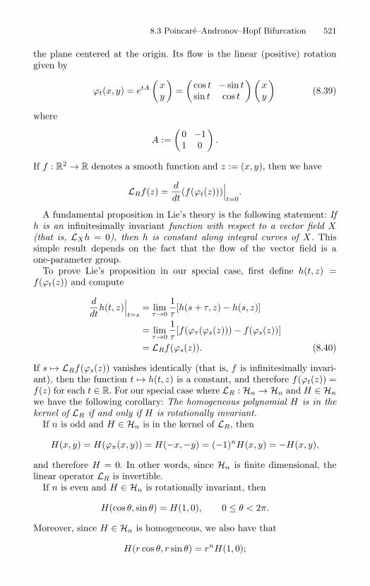
8.3 Poincare–Andronov–Hopf Bifurcation 521
the plane centered at the origin. Its flow is the linear (positive) rotationgiven by
ϕt(x, y) = etA
(xy
)=
(cos t − sin tsin t cos t
)(xy
)(8.39)
where
A :=(
0 −11 0
).
If f : R2 → R denotes a smooth function and z := (x, y), then we have
LRf(z) =d
dt(f(ϕt(z)))
∣∣∣t=0
.
A fundamental proposition in Lie’s theory is the following statement: Ifh is an infinitesimally invariant function with respect to a vector field X(that is, LXh = 0), then h is constant along integral curves of X. Thissimple result depends on the fact that the flow of the vector field is aone-parameter group.
To prove Lie’s proposition in our special case, first define h(t, z) =f(ϕt(z)) and compute
d
dth(t, z)
∣∣∣t=s
= limτ→0
1τ
[h(s + τ, z) − h(s, z)]
= limτ→0
1τ
[f(ϕτ (ϕs(z))) − f(ϕs(z))]
= LRf(ϕs(z)). (8.40)
If s → LRf(ϕs(z)) vanishes identically (that is, f is infinitesimally invari-ant), then the function t → h(t, z) is a constant, and therefore f(ϕt(z)) =f(z) for each t ∈ R. For our special case where LR : Hn → Hn and H ∈ Hn
we have the following corollary: The homogeneous polynomial H is in thekernel of LR if and only if H is rotationally invariant.
If n is odd and H ∈ Hn is in the kernel of LR, then
H(x, y) = H(ϕπ(x, y)) = H(−x,−y) = (−1)nH(x, y) = −H(x, y),
and therefore H = 0. In other words, since Hn is finite dimensional, thelinear operator LR is invertible.
If n is even and H ∈ Hn is rotationally invariant, then
H(cos θ, sin θ) = H(1, 0), 0 ≤ θ < 2π.
Moreover, since H ∈ Hn is homogeneous, we also have that
H(r cos θ, r sin θ) = rnH(1, 0);
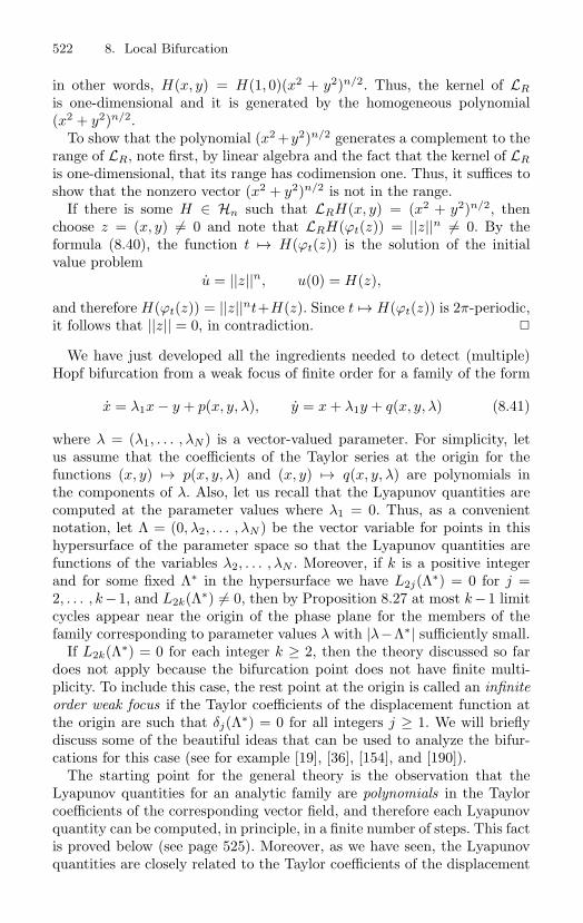
522 8. Local Bifurcation
in other words, H(x, y) = H(1, 0)(x2 + y2)n/2. Thus, the kernel of LR
is one-dimensional and it is generated by the homogeneous polynomial(x2 + y2)n/2.
To show that the polynomial (x2 +y2)n/2 generates a complement to therange of LR, note first, by linear algebra and the fact that the kernel of LR
is one-dimensional, that its range has codimension one. Thus, it suffices toshow that the nonzero vector (x2 + y2)n/2 is not in the range.
If there is some H ∈ Hn such that LRH(x, y) = (x2 + y2)n/2, thenchoose z = (x, y) = 0 and note that LRH(ϕt(z)) = ||z||n = 0. By theformula (8.40), the function t → H(ϕt(z)) is the solution of the initialvalue problem
u = ||z||n, u(0) = H(z),
and therefore H(ϕt(z)) = ||z||nt+H(z). Since t → H(ϕt(z)) is 2π-periodic,it follows that ||z|| = 0, in contradiction.
We have just developed all the ingredients needed to detect (multiple)Hopf bifurcation from a weak focus of finite order for a family of the form
x = λ1x − y + p(x, y, λ), y = x + λ1y + q(x, y, λ) (8.41)
where λ = (λ1, . . . , λN ) is a vector-valued parameter. For simplicity, letus assume that the coefficients of the Taylor series at the origin for thefunctions (x, y) → p(x, y, λ) and (x, y) → q(x, y, λ) are polynomials inthe components of λ. Also, let us recall that the Lyapunov quantities arecomputed at the parameter values where λ1 = 0. Thus, as a convenientnotation, let Λ = (0, λ2, . . . , λN ) be the vector variable for points in thishypersurface of the parameter space so that the Lyapunov quantities arefunctions of the variables λ2, . . . , λN . Moreover, if k is a positive integerand for some fixed Λ∗ in the hypersurface we have L2j(Λ∗) = 0 for j =2, . . . , k−1, and L2k(Λ∗) = 0, then by Proposition 8.27 at most k −1 limitcycles appear near the origin of the phase plane for the members of thefamily corresponding to parameter values λ with |λ−Λ∗| sufficiently small.
If L2k(Λ∗) = 0 for each integer k ≥ 2, then the theory discussed so fardoes not apply because the bifurcation point does not have finite multi-plicity. To include this case, the rest point at the origin is called an infiniteorder weak focus if the Taylor coefficients of the displacement function atthe origin are such that δj(Λ∗) = 0 for all integers j ≥ 1. We will brieflydiscuss some of the beautiful ideas that can be used to analyze the bifur-cations for this case (see for example [19], [36], [154], and [190]).
The starting point for the general theory is the observation that theLyapunov quantities for an analytic family are polynomials in the Taylorcoefficients of the corresponding vector field, and therefore each Lyapunovquantity can be computed, in principle, in a finite number of steps. This factis proved below (see page 525). Moreover, as we have seen, the Lyapunovquantities are closely related to the Taylor coefficients of the displacement
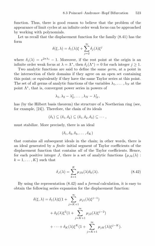
8.3 Poincare–Andronov–Hopf Bifurcation 523
function. Thus, there is good reason to believe that the problem of theappearance of limit cycles at an infinite order weak focus can be approachedby working with polynomials.
Let us recall that the displacement function for the family (8.41) has theform
δ(ξ, λ) = δ1(λ)ξ +∞∑
j=2
δj(λ)ξj
where δ1(λ) = e2πλ1 − 1. Moreover, if the rest point at the origin is aninfinite order weak focus at λ = Λ∗, then δj(Λ∗) = 0 for each integer j ≥ 1.
Two analytic functions are said to define the same germ, at a point inthe intersection of their domains if they agree on an open set containingthis point; or equivalently if they have the same Taylor series at this point.The set of all germs of analytic functions of the variables λ1, . . . , λN at thepoint Λ∗, that is, convergent power series in powers of
λ1, λ2 − λ∗2, . . . , λN − λ∗
N ,
has (by the Hilbert basis theorem) the structure of a Noetherian ring (see,for example, [24]). Therefore, the chain of its ideals
(δ1) ⊆ (δ1, δ2) ⊆ (δ1, δ2, δ3) ⊆ · · · ,
must stabilize. More precisely, there is an ideal
(δ1, δ2, δ3, . . . , δK)
that contains all subsequent ideals in the chain; in other words, there isan ideal generated by a finite initial segment of Taylor coefficients of thedisplacement function that contains all of the Taylor coefficients. Hence,for each positive integer J , there is a set of analytic functions µJk(λ) :k = 1, . . . , K such that
δJ(λ) =K∑
k=1
µJk(λ)δk(λ). (8.42)
By using the representation (8.42) and a formal calculation, it is easy toobtain the following series expansion for the displacement function:
δ(ξ, λ) = δ1(λ)ξ(1 +∞∑
j=K+1
µj1(λ)ξj−1)
+ δ2(λ)ξ2(1 +∞∑
j=K+1
µj2(λ)ξj−2)
+ · · · + δK(λ)ξK(1 +∞∑
j=K+1
µjK(λ)ξj−K).
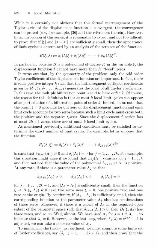
524 8. Local Bifurcation
While it is certainly not obvious that this formal rearrangement of theTaylor series of the displacement function is convergent, the convergencecan be proved (see, for example, [36] and the references therein). However,by an inspection of this series, it is reasonable to expect and not too difficultto prove that if |ξ| and |λ − λ∗| are sufficiently small, then the appearanceof limit cycles is determined by an analysis of the zero set of the function
B(ξ, λ) := δ1(λ)ξ + δ2(λ)ξ2 + · · · + δK(λ)ξK .
In particular, because B is a polynomial of degree K in the variable ξ, thedisplacement function δ cannot have more than K “local” zeros.
It turns out that, by the symmetry of the problem, only the odd orderTaylor coefficients of the displacement function are important. In fact, thereis some positive integer k such that the initial segment of Taylor coefficientsgiven by (δ1, δ3, δ5, . . . , δ2k+1) generates the ideal of all Taylor coefficients.In this case, the multiple bifurcation point is said to have order k. Of course,the reason for this definition is that at most k local limit cycles can appearafter perturbation of a bifurcation point of order k. Indeed, let us note thatthe origin ξ = 0 accounts for one zero of the displacement function and eachlimit cycle accounts for two zeros because such a limit cycle must cross boththe positive and the negative ξ-axis. Since the displacement function hasat most 2k + 1 zeros, there are at most k local limit cycles.
As mentioned previously, additional conditions must be satisfied to de-termine the exact number of limit cycles. For example, let us suppose thatthe function
B1(λ, ξ) := δ1(λ) + δ2(λ)ξ + · · · + δ2k+1(λ)ξ2k
is such that δ2k+1(Λ1) > 0 and δj(Λ1) = 0 for j = 1, . . . , 2k. For example,this situation might arise if we found that L2j(Λ1) vanishes for j = 1, . . . kand then noticed that the value of the polynomial L2k+2 at Λ1 is positive.At any rate, if there is a parameter value Λ2 so that
δ2k+1(Λ2) > 0, δ2k(Λ2) < 0, δj(Λ2) = 0
for j = 1, . . . , 2k − 1, and |Λ2 − Λ1| is sufficiently small, then the functionξ → B1(ξ,Λ2) will have two zeros near ξ = 0, one positive zero and onezero at the origin. By continuity, if |Λ3 − Λ2| is sufficiently small, then thecorresponding function at the parameter value Λ3 also has continuationsof these zeros. Moreover, if there is a choice of Λ3 in the required opensubset of the parameter space such that δ2k−1(Λ3) > 0, then B1(ξ,Λ3) hasthree zeros, and so on. Well, almost. We have used Λj for j = 1, 2, 3, . . . toindicate that λ1 = 0. However, at the last step, where δ1(λ) = e2πλ1 − 1 isadjusted, we can take a nonzero value of λ1.
To implement the theory just outlined, we must compute some finite setof Taylor coefficients, say δj : j = 1, . . . , 2k + 1, and then prove that the
8.3 Poincare–Andronov–Hopf Bifurcation 525
ideal generated by these Taylor coefficients contains all subsequent Taylorcoefficients. This is a difficult problem that has only been solved in a fewspecial cases. The most famous result of this type was proved by NikolaiN. Bautin [19] for quadratic systems—that is, for
x = εx − y + p(x, y), y = x + εy + q(x, y)
where p and q are homogeneous quadratic polynomials and where λ is thevector consisting of ε and the coefficients of p and q. In this case, Bautinshowed that the ideal of all Taylor coefficients is generated by (δ1, δ3, δ5, δ7).Thus, at most three limit cycles can bifurcate from the origin. Moreover,it is possible to construct an example where three limit cycles do appear(see [19] and [190]).
From the above remarks, it should be clear that it is not easy to countthe exact number of limit cycles of a polynomial system. Indeed, this is thecontent of Hilbert’s 16th problem: Is there a bound for the number of limitcycles of a polynomial system in terms of the degrees of the polynomialsthat define the system? This problem is not solved, even for quadratic sys-tems. The best result obtained so far is the following deep theorem of YuriIl’yashenko [97].
Theorem 8.40. A polynomial system has at most a finite number of limitcycles.
(See the book of Il’yashenko [97] and the review [30] for a mathematicalhistory of the work on Hilbert’s problem, and see [145] for a completebibliography of quadratic systems theory.)
The remainder of this section is devoted to the promised proof thatthe Lyapunov quantities for an analytic system are polynomials in theTaylor coefficients of the vector field corresponding to the system and toa description of an algorithm that can be used to compute the Lyapunovquantities.
Consider the vector field
X(x, y) := (−y∂
∂x+ x
∂
∂y) +
( ∞∑j=2
pj(x, y)∂
∂x+
∞∑j=2
qj(x, y)∂
∂y
)
where pj , qj ∈ Hj for each integer j ≥ 1. Also, let
V (x, y) :=12(x2 + y2) +
∞∑j=3
Vj(x, y)
526 8. Local Bifurcation
where Vj ∈ Hj for each j ≥ 1. The Lie derivative of V in the direction Xis given by
LXV =∞∑
j=3
LRVj + x∞∑
j=2
pj + y∞∑
j=2
qj +∞∑
j=2
pj
∞∑j=3
Vjx +∞∑
j=2
qj
∞∑j=3
Vjy
=∞∑
j=3
LRVj +∞∑
j=2
(xpj + yqj) +∞∑
j=2
( j−2∑i=0
pj−iV(i+3)x + qj−iV(i+3)y)
= LRV3 + xp2 + yq2 +∞∑
j=4
(LRVj + xpj−1 + yqj−1
+j−4∑i=0
pj−i−2V(i+3)x + qj−i−2V(i+3)y).
For each even integer j ≥ 2, let Πj : Hj → Hj denote the linear projec-tion whose kernel is the range of the operator LR and whose range is ourone-dimensional complement to the range of the operator LR; that is, thesubspace of H2j generated by the vector (x2 + y2)j . Also, for each integerj ≥ 4, define Hj ∈ Hj by
Hj := xpj−1 + yqj−1 +j−4∑i=0
(pj−i−2V(i+3)x + qj−i−2V(i+3)y
)so that
LXV = LRV3 + xp2 + yq2 +∞∑
j=4
(LRVj + Hj
).
The following algorithm can be used to compute the Lyapunov quantities:
Input (k, p2, . . . , p2k−1, q2, . . . , q2k−1)V3 := −L−1
R (xp2 + yq2)For j from 4 to 2k do
If j is odd, then Vj := −L−1R (xpj−1 + yqj−1 + Hj)
If j is even, thenLj := Πj(Hj)/(x2 + y2)j/2
Vj := −L−1R
(Hj − Lj(x2 + y2)j/2
)End for loop;Output (L4, L6, . . . , L2k).
To implement the algorithm, it is perhaps best to first choose a basis foreach vector space Hj and then to represent the linear transformations Πj
and LR in this basis (see Exercise (8.42)).
8.3 Poincare–Andronov–Hopf Bifurcation 527
Remark 4. The value of L4 in case
pj(x, y) =j∑
i=0
aj−i,ixj−iyi, qj(x, y) =
j∑i=0
bj−i,ixj−iyi
is given by
L4 =18(a20a11 + b21 + 3a30 − b02b11
+ 3b03 + 2b02a02 − 2a20b20 − b20b11 + a12 + a02a11). (8.43)
The sign of this quantity is the same as the sign of the third Taylor coef-ficient of the displacement function. Thus, the sign of L4 can be used todetermine the stability of a weak focus as required in the Hopf bifurcationtheorem.
Finally, we will show that if k is a positive integer, then the Lyapunovquantity L2k is a polynomial in the Taylor coefficients of p and q at theorigin. To prove this fact, note that
LRV2k + H2k − L2k(x2 + y2)k = 0.
Moreover, the linear flow of the vector field R is given by
ϕt(x, y) = etA
(xy
)where A =
(0 −11 0
),
and, by Exercise (8.41), the projection Π2k is represented by
Π2kH(x, y) =12π
∫ 2π
0H(ϕt(x, y)) dt. (8.44)
Since the rotationally invariant elements of H2k are in the complementof the range of LR, the composition Π2kLR is equal to the zero operator,and therefore
L2k(x2 + y2)k = Π2kH2k(x, y).
In particular, the desired Lyapunov quantity is given by the integral
L2k =12π
∫ 2π
0Hk(cos t, sin t) dt.
Hence, by inspection of the algorithm for computing the Lyapunov quanti-ties, it is clear that L2k is a polynomial in the coefficients of the polynomials
p2, . . . , p2k−1, q2, . . . , q2k−1.
528 8. Local Bifurcation
Exercise 8.41. Demonstrate that the representation (8.44) is valid by showing:a) Π2k is linear, b) Π2kH is rotationally invariant, and c) Π2k(x2 + y2)k = (x2 +y2)k.
Exercise 8.42. Show that xn−iyi | i = 0, . . . , n is a basis for Hn and LR
has the following (n+1)×(n+1) matrix representation with respect to the given(ordered) basis:
LR =
0 1 0 0 0 · · ·−n 0 2 0 0 · · ·0 1 − n 0 3 0 · · ·0 0 2 − n 0 4 · · ·· · · · · · · ·
.
Also, the kernel of LR on H2n, for n ≥ 2, is generated by the vector
K = (Bn,0, 0, Bn,1, 0, Bn,2, . . . , 0, Bn,n)
where the numbers
Bn,j =n!
j!(n − j)!
are the binomial coefficients, and
(a1, . . . , an, 0) : (a1, . . . , an) ∈ Rn
is a vector space complement to the kernel. If LR on H2n is represented bythe matrix (1, . . . , n+1) partitioned by the indicated columns, then show thatthe matrix representation for LR, restricted to the complement of the kernel,is represented by (1, . . . , n, 0). Also, consider the equation LRV = H whereV, H ∈ Hj and the associated matrix equation
(1, . . . , n, K)H = K.
Show that the matrix (1, . . . , n, K) is invertible and that H has the form H =∑ajj + LK where L is the corresponding Lyapunov quantity.
Exercise 8.43. Determine the stability of the rest point at the origin for thesystem
x = −y − x2 + xy, y = x + 2xy.
Exercise 8.44. Discuss the Hopf bifurcation for the following systems:
1. x = εx − y − x2 + xy, y = x + εy + 2xy.
2. x = εx − y − x2 + εxy, y = x + εy + 2y2.
3. x = x(x − βy) + εy, y = y(x2 − y).
Exercise 8.45. Consider the quadratic system in Bautin normal form:
x = λ1x − y − λ3x2 + (2λ2 + λ5)xy + λ6y
2,
y = x + λ1y + λ2x2 + (2λ3 + λ4)xy − λ2y
2.
Find the corresponding Lyapunov quantities L2, L4, and L6. Construct a curve inthe parameter space with a supercritical Hopf bifurcation. Construct a quadraticsystem with two limit cycles surrounding the origin and a quadratic system withthree limit cycles surrounding the origin. (If you need help, see [37][141, p. 449].)
8.3 Poincare–Andronov–Hopf Bifurcation 529
Exercise 8.46. The family
θ + sin θ − Ωcos θ sin θ = Iθ,
where Ω and I are real parameters, is a simple model in dimensionless form ofa whirling pendulum with a feedback control. Discuss the existence of a Hopfbifurcation for the rest point at the origin in the phase plane at the controlcoefficient value I = 0. How does the existence of a Hopf bifurcation depend onthe rotation speed Ω? Draw the bifurcation diagram.
Exercise 8.47. Consider the following model for the dimensionless concentra-tions x and y of certain reacting chemicals
x = a − x − 4xy
1 + x2 , y = bx(1 − y
1 + x2
),
and the curve C in the first quadrant of the (a, b)-parameter space given byb = 3a/5−25/a. Prove that a supercritical Hopf bifurcation occurs when a curvein the parameter space crosses C from above. This exercise is taken from [172, p.256] where the derivation of the model and typical phase portraits are described.
References
[1] Abraham, R. and J. E. Marsden (1978). Foundations of Mechanics,2nd ed. Reading: The Benjamin/Cummings Pub. Co.
[2] Abraham, R., J. E. Marsden, and T. Ratiu (1988). Manifolds, TensorAnalysis, and Applications, 2nd ed. New York: Springer-Verlag.
[3] Abraham, R. and J. Robbin (1967). Transversal Mappings and Flows.New York: W. A. Benjamin, Inc.
[4] Andersen, C. and J. Geer (1982). Power series expansions for fre-quency and period of the limit cycle of the van der Pol equation.SIAM J. Appl. Math. 42, 678–693.
[5] Andronov, A. A., E. A. Leontovich, I. I. Gordon, and A. G. Maier(1973). Qualitative Theory of Second-Order Dynamic Systems. NewYork: John Wiley & Sons.
[6] Andronov, A. A., E. A. Leontovich, I. I. Gordon, and A. G. Maier(1973). Theory of Bifurcations of Dynamic Systems on a Plane. NewYork: John Wiley & Sons.
[7] Andronov, A. A., A. A. Vitt, and S. E. Khaiken (1966). Theory ofOscillators. Oxford: Pergamon Press.
[8] Arnold, V. I. (1973). Ordinary Differential Equations. Cambridge:M. I. T. Press.
532 References
[9] Arnold, V. I. (1982). Geometric Methods in the Theory of OrdinaryDifferential Equations. New York: Springer-Verlag.
[10] Arnold, V. I. (1978). Mathematical Methods of Celestial Mechanics.New York: Springer-Verlag.
[11] Arnold, V. I., ed. (1988). Dynamical Systems I. New York: Springer-Verlag.
[12] Arnold, V. I., ed. (1988). Dynamical Systems III. New York: Springer-Verlag.
[13] Arnold, V. I., ed. (1990). Huygens and Barrow, Newton and Hooke,E. J. F. Primrose, trans. Basel: Birkhauser-Verlag.
[14] Arnold, V. I. and B. A. Khesin (1998). Topological Methods inHydrodynamics. New York: Springer-Verlag.
[15] Aronson D. G. and H. F. Weinberger (1978). Multidimensional non-linear diffusion arising in population genetics. Adv. Math. 30, 33–76.
[16] Ashbaugh, M., C. Chicone, and R. Cushman (1991). The twistingtennis racket. J. of Dyn. and Diff. Eqs. 3, 67–85.
[17] Barrow-Green, J. (1997). Poincare and the Three Body Problem.Providence: Amer. Math. Soc.
[18] Bates, L. M. and R. H. Cushman (1997). Global Aspects of ClassicalIntegrable Systems. Boston: Birkhauser-Verlag.
[19] Bautin, N. N. (1954). On the number of limit cycles which appearwith the variation of coefficients from an equilibrium position of focusor center type. Amer. Math. Soc. Transl. 100, 1–19.
[20] Bender, J. (1997). Chaotic dynamics in a planar Hamiltonian system.Master’s Project. Columbia: University of Missouri.
[21] Benguria, R. D. and M. C. Depassier (1996). Variational characteri-zation of the speed of propagation of fronts for the nonlinear diffusionequation. Comm. Math. Phy. 175, 221–227.
[22] Bisplinghoff, R. L. and H. Ashley (1975). Principles of Aeroelasticity.New York: Dover Publications, Inc.
[23] Bogoliubov, N. N. and Y. A. Mitropolsky (1961). Asymptotic Meth-ods in the Theory of Nonlinear Oscillations. Delhi: Hindustan Pub.Corp.
[24] Brieskorn, E. and H. Knorrer (1986). Plane Algebraic Curves. Basel:Birkhauser-Verlag.
References 533
[25] Byrd, P. F. and M. D. Friedman (1971). Handbook of Elliptic Integralsfor Engineers and Scientists, 2nd ed. Berlin: Springer-Verlag.
[26] Caratheodory, C. (1954). Theory of Functions of a Complex Variable,1, pp. 229–236. New York: Chelsea.
[27] Chen, M., X.–Y. Chen, and J. K. Hale (1992). Structural stabilityfor time-periodic one-dimensional parabolic equations. J. Diff. Eqs.96(2), 355–418.
[28] Chicone, C. (1986). Limit cycles of a class of polynomial vector fieldsin the plane. J. Diff. Eqs. 63(1), 68–87.
[29] Chicone, C. (1987). The monotonicity of the period function for pla-nar Hamiltonian vector fields. J. Diff. Eqs. 69, 310–321.
[30] Chicone, C. (1993). review of Finiteness Theorems for Limit Cycles,by Yu. Il’yashenko. Bull. Amer. Math. Soc. 28(1), 123–130.
[31] Chicone, C. (1992). Bifurcation of nonlinear oscillations and fre-quency entrainment near resonance. SIAM J. Math. Anal. 23(6),1577–1608.
[32] Chicone, C. (1994). Lyapunov–Schmidt reduction and Melnikov in-tegrals for bifurcation of periodic solutions in coupled oscillators. J.Diff. Eqs. 112, 407–447.
[33] Chicone, C. (1995). A geometric approach to regular perturbationtheory with an application to hydrodynamics. Trans. Amer. Math.Soc. 374(12), 4559–4598.
[34] Chicone, C. (1997). Invariant tori for periodically perturbed oscilla-tors. Publ. Mat. 41, 57–83.
[35] Chicone, C. and F. Dumortier (1993). Finiteness for critical points ofthe period function for analytic vector fields on the plane. NonlinearAnaly. 20(4), 315-335.
[36] Chicone, C. and M. Jacobs (1989). Bifurcation of critical periods forplane vector fields. Trans. Amer. Math. Soc. 312, 433–486.
[37] Chicone, C. and M. Jacobs (1991). Bifurcation of limit cycles fromquadratic isochrones. J. of Diff. Eqs. 91, 268–327.
[38] Chicone, C. and Yu. Latushkin (1997). The geodesic flow generates afast dynamo: an elementary proof. Proc. Amer. Math. Soc. 125(11),3391–3396.

534 References
[39] Chicone, C. and Yu. Latushkin (1999). Evolution Semigroups in Dy-namical Systems and Differential Equations. Providence: AmericanMathematical Society.
[40] Chicone, C. and W. Liu (1999). On the continuation of an invarianttorus in a family with rapid oscillation. SIAM J. Math. Analy. Toappear.
[41] Chicone, C., B. Mashhoon, and D. G. Retzloff (1996). Gravitationalionization: periodic orbits of binary systems perturbed by gravita-tional radiation. Ann. Inst. H. Poincare. 64(1), 87–125.
[42] Chicone, C., B. Mashhoon, and D. G. Retzloff (1996). On the ioniza-tion of a Keplerian binary system by periodic gravitational radiation.J. Math Physics. 37, 3997–1416.
[43] Chicone, C., B. Mashhoon, and D. G. Retzloff (1997). Addendum: Onthe ionization of a Keplerian binary system by periodic gravitationalradiation. J. Math Physics. 38(1), 554.
[44] Chicone, C., B. Mashhoon, and D. G. Retzloff (1997). Gravitationalionization: a chaotic net in the Kepler system. Class. Quantum Grav.14, 699–723.
[45] Chicone, C., B. Mashhoon, and D. G. Retzloff (1999). Chaos in theKepler system. Class. Quantum Grav. 16, 507–527.
[46] Chicone, C. and J. Sotomayor (1986). On a class of complete poly-nomial vector fields in the plane. J. Diff. Eqs. 61(3), 398–418.
[47] Chicone, C. and J. Tian (1982). On general properties of quadraticsystems. Proc. Amer. Math. Soc. 89(3), 167–178.
[48] Chorin, A. J. and J. E. Marsden (1990). A Mathematical Introductionto Fluid Mechanics, 2nd ed. New York: Springer-Verlag.
[49] Chow, S. N. and J. K. Hale (1982). Methods of Bifurcation Theory.New York: Springer-Verlag.
[50] Chow, S. N., C. Li, and D. Wang (1994). Normal Forms and Bi-furcation of Planar Vector Fields. Cambridge: Cambridge UniversityPress.
[51] Coddington, E. A. and N. Levinson (1955). Theory of Ordinary Dif-ferential Equations. New York: McGraw–Hill Book Co.
[52] Colwell, P. (1992). Bessel functions and Kepler’s equation. Amer.Math. Monthly. 99, 45–48.
References 535
[53] Coppel, W. A. (1960). On a differential equation of boundary-layertheory. Phil. Trans. Roy. Soc. London, Ser. A. 253, 101–36.
[54] Dadfar, M., J. Geer, and C. Andersen (1984). Perturbation analysisof the limit cycle of the free van der Pol equation. SIAM J. Appl.Math. 44, 881–895.
[55] Davenport, J. H., Y. Siret, and E. Tournier (1993). Computer Al-gebra: Systems and Algorithms for Algebraic Computation, 2nd ed.London: Academic Press, Ltd.
[56] Diacu, F. and P. Holmes (1996). Celestial Encounters : The Originsof Chaos and Stability. Princeton: Princeton University Press.
[57] Diliberto, S. P. (1950). On systems of ordinary differential equations.In Contributions to the Theory of Nonlinear Oscillations, Annals ofMathematics Studies, 20, pp. 1–38. Princeton: Princeton UniversityPress.
[58] Dumortier, F. (1977). Singularities of vector fields on the plane. J.Diff. Eqs. 23(1), 53–106.
[59] Dumortier, F. (1978). Singularities of Vector Fields. Rio de Janeiro:IMPA Monograph, No. 32.
[60] Dunford, N. and J. T. Schwartz (1958). Linear Operators. New York:Interscience Publications, Inc.
[61] Ewing, G. M. (1969). Calculus of Variations with Applications. NewYork: W. W. Norton & Company, Inc.
[62] Falkner, V. M. and S. W. Skan (1931). Solution of boundary layerequations. Philos. Mag. 7(12), 865–896.
[63] Farkas, M. (1994). Periodic Motions. New York: Springer-Verlag.
[64] Fenichel, N. (1971). Persistence and smoothness of invariant mani-folds for flows. Indiana U. Math. J. 21, 193–226.
[65] Fermi, E., S. Ulam, and J. Pasta (1974). Studies of nonlinear prob-lems I. In Nonlinear Wave Motion, Lect. Appl. Math., Amer. Math.Soc. 15, 143–155.
[66] Feynman, R. P., R. B. Leighton, and M. Sands (1964). The FeynmanLectures on Physics I–III. Reading: Addison–Wesley Pub. Co.
[67] Fife, P. C. (1979). Mathematical Aspects of Reacting and DiffusingSystems. Lect. Notes Biomath., 28. New York: Springer-Verlag.

536 References
[68] Flanders, H. (1963). Differential Forms with Applications to thePhysical Sciences. New York: Dover Publicaitions, Inc.
[69] Fletcher, C. A. J. (1982). Burgers’ equation: a model for all reasons.In Numerical Solutions of Partial Differential Equations. J. Noye, ed.Amsterdam: North–Holland Pub. Co.
[70] Friedlander, S., A. Gilbert, and M. Vishik (1993). Hydrodynamicinstability and certain ABC flows. Geophys. Astrophys. Fluid Dyn.73(1-4), 97–107.
[71] Friedrich, H. and D. Wintgen, (1989). The hydrogen atom in a uni-form magnetic field—an example of chaos. Phys. Reports. 183(1),37–79.
[72] Geyling, F. T. and H. R. Westerman (1971). Introduction to OrbitalMechanics. Reading: Addison–Wesley Pub. Co.
[73] Ghil, M. and S. Childress (1987). Topics in Geophysical Fluid Dy-namics : Atmospheric Dynamics, Dynamo Theory, and Climate Dy-namics. New York: Springer-Verlag.
[74] Golubitsky, M. and D. G. Schaeffer (1985). Singularities and Groupsin Bifurcation Theory, 1. New York: Springer-Verlag.
[75] Golubitsky, M., I. Stewart, and D.G. Schaeffer (1988). Singularitiesand Groups in Bifurcation Theory, 2. New York: Springer-Verlag.
[76] Gonzales, E. A. (1969). Generic properties of polynomial vector fieldsat infinity. Trans. Amer. Math. Soc. 143, 201–222.
[77] Greenspan, B and P. Holmes (1984). Repeated resonance and homo-clinic bifurcation in a periodically forced family of oscillators. SIAMJ. Math. Analy. 15, 69–97.
[78] Grimshaw, R. (1990). Nonlinear Ordinary Differential Equations.Oxford: Blackwell Scientific Pub.
[79] Grobman, D. (1959). Homeomorphisms of systems of differentialequations (Russian). Dokl. Akad. Nauk. 128, 880–881.
[80] Guckenheimer, J. and P. Holmes (1986). Nonlinear Oscillations, Dy-namical Systems, and Bifurcations of Vector Fields, 2nd ed. NewYork: Springer-Verlag.
[81] Gutierrez, C. (1995). A solution to the bidimensional global asymp-totic stability conjecture. Ann. Inst. H. Poincare Anal. Non Lineaire.12(6), 627–671.
References 537
[82] Gutzwiller, M. C. (1990). Chaos in Classical and Quantum Mechan-ics. New York: Springer-Verlag.
[83] Hale, J. K. (1980). Ordinary Differential Equations, 2nd ed. Malabar:R. E. Krieger Pub. Co.
[84] Hale, J. K., L.T. Magalhaes, and W. M. Oliva (1984). An Introduc-tion to Infinite Dimensional Dynamical Systems—Geometric Theory.New York: Springer-Verlag.
[85] Hale, J. K. (1988). Asymptotic Behavior of Dissipative Systems.Providence: American Mathematical Society.
[86] Hall, R. (1984). Resonance zones in two-parameter families of circlehomeomorphisms. SIAM J. Math. Analy. 15, 1075–1081.
[87] Hartman, P. (1960). A lemma in the theory of structural stability ofdifferential equations. Proc. Amer. Math. Soc. 11, 610–620.
[88] Hastings, S. P. and W. C. Troy (1988). Oscillating solutions of theFalkner–Skan equation for positive β. J. Diff. Eqs. 71, 123–144.
[89] Hayashi, C. (1964). Nonlinear Oscillations in Physical Systems. NewYork: McGraw–Hill Book Co.
[90] Henry, D. (1981). Geometric Theory of Semilinear Parabolic Equa-tions. New York: Springer-Verlag.
[91] Howe, R. (1983). Very basic Lie theory. Amer. Math. Monthly. 90,600–623; Correction (1984). 91, 247.
[92] Hirsch, M. (1976). Differential Topology. New York: Springer-Verlag.
[93] Hirsch, M. and C. Pugh (1970). Stable manifolds and hyperbolic sets.In Global Analysis XIV, Amer. Math. Soc. 133–164.
[94] Hirsch, M., C. Pugh, and M. Shub (1977). Invariant Manifolds, Lec-ture Notes in Math., 583. New York: Springer-Verlag.
[95] Hirsch, M. and S. Smale (1974). Differential Equations, DynamicalSystems, and Linear Algebra. New York: Academic Press.
[96] Holmes, P. and J. Marsden (1981). A partial differential equationwith infinitely many periodic orbits and chaotic oscillations of aforced beam. Arch. Rat. Mech. Analy. 76, 135–165.
[97] Il’yashenko, Yu. S. (1991). Finiteness Theorems for Limit Cycles,Transl. Math. Mono., 94. Providence: American Mathatematical So-ciety.
538 References
[98] Iooss, G. and M. Adelmeyer (1992). Topics in Bifurcation Theoryand Applications. River Edge: World Scientific Pub. Company, Inc.
[99] Isaacson, E and H. Keller (1966). Analysis of Numerical Methods.New York: John Wiley & Sons, Inc.
[100] Katok, A. B and B. Hasselblatt (1995). Introduction to the Mod-ern Theory of Dynamical Systems. Cambridge: Cambridge UniversityPress.
[101] Kevorkian, J. and J. D. Cole (1981). Perturbation Methods in AppliedMathematics. New York: Springer-Verlag.
[102] Kovalevsky, J. (1967). Introduction to Celestial Mechanics, Astro-physics and Space Science Library, 7. New York: Springer-Verlag.
[103] Kolmogorov, A. N., I. G. Petrovskii, and N. S. Piskunov (1991). Astudy of the diffusion equation with increase in the amount of sub-stance, and its applications to a biological problem. In Selected Worksof A. N. Kolmogorov, V. M. Tikhomirov, ed. Dordrecht: Kluwer Aca-demic Pub. Group.
[104] Landau, L. D. and E. M. Lifshitz (1951). Classical Theory of Fields.Reading: Addison–Wesley Press.
[105] Landau L. D. and E. M. Lifshitz (1987). Fluid Mechanics, 2nd ed.,J. B. Sykes and W. H. Reid, trans. New York: Pergamon Press.
[106] Lang, S. (1962). Introduction to Differentiable Manifolds. New York:Interscience Pub.
[107] Lefschetz, S. (1977). Differential Equaitions: Geometric Theory, 2nded. New York: Dover Publications, Inc.
[108] Levi, M. (1988). Stability of the inverted pendulum—a topologicalexplanation. SIAM Rev. 30, 639–644.
[109] Levi, M., C. Hoppensteadt, and M. Miranker (1978). Dynamics ofthe Josephson junction. Quart. Appl. Math. 36, 167–198.
[110] Lochak, P. and C. Meunier (1988). Multiphase Averaging for ClassicalSystems, H. S. Dumas, trans. New York: Springer-Verlag.
[111] Lorenz, E. N. (1963). Deterministic non-periodic flow. J. Atmos. Sci.20, 131–141.
[112] Loud, W. S. (1964). Behavior of the periods of solutions of certainplane autonomous systems near centers. Contributions Diff. Eqs. 3,21–36.
References 539
[113] Lichtenberg, A. J. and M. A. Lieberman (1982). Regular and Stochas-tic Motion. New York: Springer-Verlag.
[114] Liapounoff, M. A. (1947). Probleme general de la stabilite du move-ment. Princeton: Princeton University Press.
[115] Magnus, W. and S. Winkler (1979). Hill’s Equation. New York: DoverPublications, Inc.
[116] Massey, W. S. (1967). Algebraic Topology: An Introduction. NewYork: Springer-Verlag.
[117] Marsden, J. E. and M. McCracken (1976). The Hopf Bifurcation andIts Applications. New York: Springer-Verlag.
[118] McCuskey, S. W. (1963). Introduction to Celestial Mechanics. Read-ing: Addison–Wesley Pub. Co.
[119] McLachlan, N. W. (1958). Ordinary Non-linear Differential Equa-tions in Engineering and Physical Sciences, 2nd ed. New York: Ox-ford University Press.
[120] Melnikov, V. K. (1963). On the stability of the center for time peri-odic perturbations. Trans. Moscow Math. Soc. 12, 1–57.
[121] Milnor, J. (1963). Morse Theory. Princeton: Princeton UniversityPress.
[122] Milnor, J. (1978). Analytic proofs of the “hairy ball theorem” and theBrouwer fixed-point theorem. Amer. Math. Monthly 85(7), 521–524.
[123] Meyer, K. R. and G. R. Hall (1992). Introduction to HamiltonianDynamical Systems and the N -Body Problem. New York: Springer-Verlag.
[124] Meyer, K. R. and D. S. Schmidt (1977). Entrainment domains. Funk-cialaj Edvacioj. 20, 171–192.
[125] Minorsky, N. (1962). Nonlinear Oscillations. Princeton: D. Van Nos-trand Company, Inc.
[126] Moser, J. (1969). On a theorem of Anosov. J. Diff. Eqns. 5, 411–440.
[127] Moser, J. (1973). Stable and Random Motions in Dynamical Systems,Annals of Math. Studies, 77. Princeton: Princeton University Press.
[128] Moser, J. (1978/79). Is the solar system stable? Math. Intelligencer1(2), 65–71.
[129] Munkres, J. R. (1975). Topology: A First Course. Englewood Cliffs:Prentice–Hall, Inc.
540 References
[130] Murdock, J. A. (1991). Perturbations: Theory and Methods. NewYork: Wiley–Interscience Pub.
[131] Murdock, J. A. and C. Robinson (1980). Qualitative dynamics fromasymptotic expansions: Local theory. J. Diff. Eqns. 36, 425–441.
[132] Murray, J. D. (1980). Mathematical Biology. New York: Springer-Verlag.
[133] Nayfeh, A. H. (1973). Perturbation Methods. New York: John Wiley& Sons.
[134] Nemytskii, V. V. and V. V. Stepanov (1989). Qualitative Theory ofDifferential Equations. New York: Dover Publications, Inc.
[135] Oden, J. T. (1979). Applied Functional Analysis: A First Course forStudents of Mechanics and Engineering Science. Englewood Cliffs:Prentice–Hall, Inc.
[136] Olver, P. J. (1986). Applications of Lie Groups to Differential Equa-tions. New York: Springer-Verlag.
[137] O’Malley, R. E. (1991). Singular Perturbation Methods for OrdinaryDifferential Equations. New York: Springer-Verlag.
[138] Palais, R. P. (1997). The symmetries of solitons. Bull. Amer. Math.Soc. 34, 339–403.
[139] Palis, J. and W. deMelo (1982). Geometric Theory of DynamicalSystems: An Introduction. New York: Springer-Verlag.
[140] Pao, C. V. (1992). Nonlinear Parabolic and Elliptic Equations. NewYork: Plenum Press.
[141] Perko, L. (1996). Differential Equations and Dynamical Systems, 2nded. New York: Springer-Verlag.
[142] Petty, C. M. and J. V. Breakwell (1960). Satellite orbits about aplanet with rotational symmetry. J. Franklin Inst. 270(4), 259–282.
[143] Poincare, H. (1881). Memoire sur les courbes definies par uneequation differentielle. J. Math. Pures et Appl. 7(3), 375–422; (1882).8, 251–296; (1885). 1(4), 167–244; (1886). 2, 151–217; all reprinted(1928). Oeuvre, Tome I. Paris: Gauthier–Villar.
[144] Pugh, C. (1969). On a theorem of P. Hartman. Amer. J. Math. 91,363–367.
[145] Reyn, J. W. (1994). A Bibliography of the Qualitative Theory ofQuadratic Systems of Differential Equations in the Plane, 3rd ed.,Tech. Report 94-02. Delft: TU Delft.
References 541
[146] Rayleigh, Lord (1883). On maintained vibrations. Phil. Mag. 15, 229.
[147] Rhouma, M. B. H. and C. Chicone (1999). On the continuation ofperiodic orbits. Meth. Appl. Analy. To appear.
[148] Robbin, J. W. (1968). On the existence theorem for differential equa-tions. Proc. Amer. Math. Soc. 19, 1005–1006.
[149] Robbin, J. W. (1981). Algebraic Kupka–Smale theory. Lecture Notesin Math. 898, 286–301.
[150] Robbin, J. W. (1972). Topological conjugacy and structural stabilityfor discrete dynamical systems. Bull. Amer. Math. Soc. 78(6), 923–952.
[151] Robinson, C. (1995). Dynamical Systems: Stability, Symbolic Dynam-ics, and Chaos. Boca Raton: CRC Press.
[152] Roberts, A. J. (1997). Low-dimensional modelling of dynamical sys-tems. http://xxx.lanl.gov/abs/chao-dyn/9705010.
[153] Rothe, F. (1993). Remarks on periods of planar Hamiltonian systems.SIAM J. Math. Anal. 24(1), 129–154.
[154] Roussarie, R. (1998). Bifurcation of Planar Vector Fields andHilbert’s Sixteenth Problem. Basel: Birkhaauser-Verlag.
[155] Rousseau, C. and B. Toni (1997). Local bifurcations of critical periodsin the reduced Kukles system. Can. J. Math. 49(2), 338–358.
[156] Rudin, W. (1966). Real and Complex Analysis. New York: McGraw–Hill Book Co.
[157] Sanders, J. A. and F. Verhulst (1985). Averaging Methods in Nonlin-ear Dynamical Systems. New York: Springer-Verlag.
[158] Schecter, S. (1990). Simultaneous equilibrium and heteroclinic bifur-cation of planar vector fields via the Melnikov integral. Nonlinearity.3, 79–99.
[159] Smale, S. (1965). Diffeomorphisms with many periodic points. InDifferential and Combinatorial Topology, S. S. Cairns, ed. Princeton:Princeton Univ. Press 63–80.
[160] Smale, S. (1980). The Mathematics of Time: Essays on Dynam-ical Systems, Economic Processes and Related Topics. New York:Springer-Verlag.
[161] Smale, S. (1998). Finding a horseshoe on the beaches of Rio. Math.Intelligencer. 20, 39–62.
542 References
[162] Smoller, J. (1980). Shock Waves and Reaction-Diffusion Equations.New York: Springer-Verlag.
[163] Sotomayor, J. (1974). Generic one-parameter families of vector fieldson two-dimensional manifolds. Publ. Math. IHES 43, 5–46.
[164] Sotomayor, J. (1979). Licoes de equacoes diferenciais ordinarias. Riode Janerio: IMPA.
[165] Sotomayor, J. (1996). Private communication. Lleida Spain.
[166] Spanier, E. H. (1981). Algebraic Topology, corrected reprint. NewYork: Springer-Verlag.
[167] Spivak, M. (1965). Calculus on Manifolds. New York: W. A. Ben-jamin, Inc.
[168] Sternberg, S. (1969). Celestial Mechanics, Parts I and II. New York:W. A. Benjamin, Inc.
[169] Stoker, J. J. (1950). Nonlinear Vibrations. New York: John Wiley &Sons.
[170] Strang, G. and G. J. Fix (1973). An Analysis of the Finite ElementMethod. Englewood Cliffs: Prentice–Hall, Inc.
[171] Strauss, W. A. (1992). Partial Differential Equations: An Introduc-tion. New York: John Wiley & Sons.
[172] Strogatz, S. (1994). Nonlinear Dynamics and Chaos. Reading:Addison–Wesley Pub. Co.
[173] Takens, F. (1974). Singularities of vector fields. Publ. Math. IHES43, 47–100.
[174] Temam, R. (1988). Infinite-dimensional Dynamical Systems in Me-chanics and Physics. New York: Springer-Verlag.
[175] Trotter, H. F. (1959). On the product of semi-groups of operators.Proc. Amer. Math. Soc. 10, 545–551.
[176] van der Pol, B. (1926). On relaxation oscillations. Phil. Mag. 2, 978–992.
[177] van der Pol, B. and J. van der Mark (1927). Frequency demultiplica-tion. Nature. 120, 363–364.
[178] van der Pol, B. and J. van der Mark (1929). The heartbeat consideredas a relaxation oscillation and an electrical model of the heart. Arch.Neerl. de Physiol. de L’homme et des Animaux. 14, 418–443.
References 543
[179] Verhulst, F. (1989). Nonlinear Differential Equations and DynamicalSystems, New York: Springer-Verlag.
[180] Watson, G. N. (1966). A Treatise on the Theory of Bessel Functions,2nd ed. Cambridge: Cambridge University Press.
[181] Weinberger, H. (1999). An example of blowup produced by equaldiffusions. J. Diff. Eqns. To appear.
[182] Weissert, T. (1997). The Genesis of Simulation in Dynamics: Pur-suing the Fermi–Ulam–Pasta Problem. New York: Springer-Verlag.
[183] Weyl, H. (1952). Space–Time–Matter, H. L. Brose, trans. New York:Dover Publications, Inc.
[184] Wiggins, S. W. (1988). Global Bifurcations and Chaos. New York:Springer-Verlag.
[185] Wiggins, S. W. (1990). Introduction to Applied Nonlinear DynamicalSystems and Chaos. New York: Springer-Verlag.
[186] Whittaker, E. T. and G. N. Watson (1927). A Course of ModernAnalysis, 1996 reprint. Cambridge: Cambridge University Press.
[187] Winkel, R. (1998). A transfer principle in the real planefrom non-singular algebraic curves to polynomial vector fields.http://www.iram.rwth-aachen.de/˜winkel/.
[188] Yagasaki, K. (1994). Chaos in a pendulum with feedback control.Nonlinear Dyn. 6, 125–142.
[189] Yakubovich, V. A. and V. M. Starzhinskii (1975). Linear DifferentialEquations with Periodic Coefficients, D. Louvish, trans. New York:John Wiley & Sons.
[190] Zoladek, H. (1994). Quadratic systems with center and their pertur-bations. J. Diff. Eqs. 109(2), 223–273.
[191] Zeidler, E. (1991). Applied Functional Analysis: Applications toMathematical Physics. New York: Springer-Verlag.
Index
ABC system, 431–449and elliptic functions, 445and chaotic attractors, 440and hydrodynamic
instability, 443and Melnikov function, 435as oscillator, 433chaotic, 434–440heteroclinic cycle for, 434numerical experiment, 440periodic orbits of, 441–449Picard–Fuchs
equation, 449unperturbed
phase portrait, 432action integral, 202, 452action-angle variables, 220
and averaging, 452and Diliberto’s theorem, 478and time map, 453for harmonic oscillator, 452for Kepler system, 207–222for planar system, 477–481
adjoint representation, 148aeroelasticity, 273
analytic function, 3Andronov, A., 317angular coordinate system, 56angular momentum, 209annular region, 83anomaly
eccentric, 218mean, 218
arc, 28Arnold
tongue, 246, 350, 372web, 466
Arnold, V., 372, 486ascending node, 210associated curve, 502asymptotic
period, 194phase, 194stability, 19
asymptotic stability, 19autonomous differential equation
change of coordinates, 52first order, 5geometry of, 6orbit types, 9
546 Index
perturbations of, 326–339phase flow, 12
autonomous differentialequation, 4
averaged systemat resonance, 462definition, 456diamagnetic Kepler, 232for satellite
of oblate planet, 227forced oscillator, 470with two angles, 468
averaging, 205, 226–233, 451–475action-angle variables, 452and celestial mechanics, 456and diffusion, 467and fundamental problem
of dynamicalsystems, 454
and integrable systems, 452and periodic orbits, 471and resonance, 454, 460
capture, 463passage through, 463, 474
and slow evolutionof action, 455
at resonance, 460pendulum model, 463–467
counterexample, 468diamagnetic
Kepler problem, 228–232disturbed binary system, 226entrainment, 475general invalidity of, 467origins of, 226partial, 462planar forced oscillator, 470principle, 455resonant
layer, 461torus, 454
theorem, 456transient chaos, 475
Baire space, 493
Baire’s theorem, 493Banach space
calculus in, 93–117integration in, 100–105
basin of attraction, 27Bautin’s theorem, 525Bautin, N., 90, 525Bender, J., 502Bendixson’s Criterion, 89Bernoulli’s equation, 53Bessel function, 222bifurcation, 10–21, 321–385, 483–
527and loss of stability, 484blue sky, 12diagram, 10function, 363, 369
identification, 321, 324, 328,337, 363, 369
reduced, 361reduction, 321, 337subharmonic, 370
Hopf, 502–527order k, 524
pitchfork, 496saddle-node, 12, 372, 484–501,
511Hamiltonian, 501
theory, 483–527and applied
mathematics, 487–489and families, 488and jets, 489–496and transversality, 489–496normal forms, 486one-dimensional
state space, 484–496transcritical, 496
big O notation, 320bilinear form
coercive, 267continuous, 267
binary systemaction-angle coordinates, 207and celestial mechanics, 207
Index 547
and fundamental problemof dynamics, 220
angular momentum, 209completely integrable, 220Delaunay elements, 215diamagnetic Kepler problem
averaging, 232diamagnetic Kepler
problem, 228–232disturbed, 215
in Delaunay elements, 219equations of motion, 206–214Euler angles, 210harmonic oscillator
model, 213invariant tori, 213, 220Kepler
ellipse, 214equation, 221third law, 215
osculating plane, 210satellite of an oblate
planet, 222–228averaging, 226critical inclination, 227
birational map, 56blow up
in finite time, 3, 4blowup
and desingularization, 64at rest point, 64–70of singularity, 64–66, 507
blue sky catastrophe, 12Bogoliubov, N., 317boundary layer, 429–431
singularperturbation, 431
boundary value problemat boundary layer, 430Dirichlet, 249Neumann, 250
branch point, 372Brouwer fixed point
theorem, 73, 77, 88bundle map, 110
Cr
function, 40-norm, 94
calculus, 93–117canonical coordinates, 228Cauchy’s
theorem, 410center, 18, 22
linear, 22center manifold, 30, 284, 299center-stable manifold, 299central projection, 67chain rule, 93change of coordinates, 53chaos
chaotic attractor, 394informal definition, 393theory, 391
Melnikov method, 391transverse homoclinic
points, 406–420transient, 394
chaotic attractor, 440Chapman–Kolmogorov
identities, 133characteristic
exponent, 167multiplier, 166
characteristicsof PDE, 279
charged particleand Lorentz force, 205motion of, 205relativistic motion, 205
Chebyshev polynomial, 282Cherkas, L., 91cocycle, 134Cole, J., 317compactification
at infinity, 66polynomial vector field, 68
completeelliptic integral, 446forward orbit, 79
complex
548 Index
potential, 428solution, 135
configuration space, 32connecting orbit, 82conservation law, 278, 281constitutive laws, 204continuable periodic orbit, 321continuation
point, 321, 334, 337, 361subharmonic, 344, 345, 363,
365, 367, 369, 370theory, 317–390
and entrainment forvan der Pol, 382
Arnold tongue, 350, 372autonomous
perturbations, 326entrainment, 367for multidimensional
oscillators, 366forced oscillators, 384forced van der Pol, 347from rest points, 343isochronous period
annulus, 343limit cycles, 367Lindstedt series, 374Lyapunov–Schmidt
reduction, 358–361Melnikov function, 339, 365nonautonomous
perturbations, 340normal nondegeneracy, 356perihelion of Mercury, 374regular period annulus, 356resonance zone, 367unforced van der Pol, 318
continuity equation, 249, 422continuous dependence
of solutions, 3contraction
constant, 106definition of, 106fiber contraction, 111mapping theorem, 106
principle, 106–116uniform, 107
convection, 249coordinate
chart, 37, 40map, 38system, 40
coordinate systemangular, 56polar, 57
coordinatescylindrical, 58polar, 56–61spherical, 58, 67
covering map, 56critical inclination, 227critical point, 9curl, 330curve, 28cut-off function, 298cylindrical coordinates, 58
degrees of freedom, 32Delaunay elements, 207desingularized vector field, 59determining equations, 380detuning parameter, 340, 371–373diagonal set, 52diamagnetic Kepler
problem, 228–232diffeomorphism, 39differentiable function, 39, 93differential
1-form, 61of function, 62
differential equationABC, see ABC systemautonomous, 4Bernoulli’s, 53binary system, 206Burgers’, 281charged particle, 205continuity, 249, 422coupled pendula, 233diffusion, 249
Index 549
Duffing’s, 273, 406Euler’s
fluid motion, 423rigid body, 35
Euler–Lagrange, 200Falkner–Skan, 431Fermi–Ulam–Pasta, 236Fisher’s, 274for fluids, see fluid dynamicsfor projectile, 86harmonic oscillator, 9heat, 249Hill’s, 179inverted pendulum, 242Lorenz, 395Loud’s, 344Mathieu, 175Maxwell’s, 203Navier–Stokes, 423Newton’s, 26, 32, 203nonautonomous, 4order of, 5ordinary, 1pendulum, see pendulumPicard–Fuchs, 449quadratic, 79reaction diffusion, 249Riccati, 183singular, 70solution of, 2spatial oscillator, 206van der Pol, 2, 5, 91, 92, 318,
405variational, 76Volterra–Lotka, 42
diffusion, 249equation, 249rates, 468
diffusivity constant, 249Diliberto, S., 331Diliberto’s theorem, 330dipole potential, 64directional derivative, 200Dirichlet problem, 249discrete dynamical system, 305
discriminant locus, 352displacement function, 73, 320, 342
reduced, 321divergence
and Bendixson’s criterion, 89and Diliberto’s theorem, 330and limit cycles, 85, 90and volume, 88
Dulaccriterion, 90function, 90, 91
eccentric anomaly, 218eigenvalue
definition of, 135eigenvalues
and adapted norms, 189and characteristic
multipliers, 167, 175and Floquet theory, 165and fundamental matrix, 137and generic bifurcation, 484and Hopf bifurcation, 502and hyperbolic
fixed points, 306and hyperbolicity, 22and index of singularity, 389and invariant manifolds, 284and Lyapunov exponents, 177and normal modes, 237and perturbation series, 347and spectrum, 252and stability, 20, 21, 127, 151,
155, 158, 275of periodic orbits, 187, 472of subharmonics, 346of time-periodic
systems, 168, 171and stability for PDE, 251continuity of, 484of derivative of
Poincare map, 187of matrix exponential, 167stability, 154
eigenvector
550 Index
definition of, 135Einstein, A., 375elliptic functions
integrals, 445Jacobi, 446
elliptic modulus, 446energy method
for PDE, 254energy surface, 32
regular, 32, 452entrainment, 349, 367–374, 382–
384, 475domain, 348, 371
equationcontinuity, 249Duffing’s, 273Falkner–Skan, 431Fisher’s, 274functional, 299, 306Kepler’s, 218, 221Lyapunov’s, 161Newton’s, 256spring, 318van der Pol, 92, 318
equilibrium point, 9ergodic, 315Euclidean space, 61, 62Euler’s equations
fluid dynamics, 423rigid body motion, 35
Euler–Lagrange equation, 200–203and extremals, 201and Hamilton’s principle, 202and Lagrangian, 202of free particle, 202
evaluation map, 98evolution
family, 133group, 133
existence theory, 1–4, 117–126by contraction, 120by implicit function
theorem, 118maximal extension, 124
smoothness by fibercontraction, 122
exponential map, 139extremal, 201
Falkner–Skan equation, 431family of differential equations, 2Farkas, M., 317fast
time, 70variable, 462
Fermi, E., 236Fermi–Ulam–Pasta
oscillator, 236–240experiments, 240normal modes, 240
Feynman, R., 203fiber
contraction, 111contraction theorem, 111of tangent bundle, 48of trivial bundle, 110
Fife, P., 278first integral, 33, 281first variational equation, 329fixed point, 106, 305
globally attracting, 106Floquet
exponent, 167normal form, 165theorem, 162theory, 162–175
and limit cycles, 170and matrix exponential, 162and periodic solutions, 172and resonance, 170characteristic exponents, 167characteristic multipliers, 165Marcus–Yamabe
example, 171monodromy operator, 165reduction to constant
system, 168flow, 13
complete, 12
Index 551
flow box theorem, 53fluid dynamics, 421–449
ABC flow, see ABC systemBernoulli’s
equation, 427law, 427
boundary conditions, 423continuity equation, 423corner flow, 429equations of motion, 422Euler’s equations, 423Falkner–Skan equation, 431flow in a pipe, 424Navier–Stokes
equations, 422plug flow, 425Poiseuille flow, 426potential flow, 427Reynold’s number, 423stream function, 428
foliation, 197forced oscillator, 384–390formal solution, 253formula
Lie–Trotter product, 145Liouville’s, 134variation of constants, 155
forward orbit, 79, 85Frechet differentiable, 93Fredholm
index, 359map, 359
frequency, 318function
Bessel, 222bifurcation, 363, 369contraction, 106differentiable, 39displacement, 73Dulac, 90exponential, 139Lipschitz, 120, 157local representation, 39Lyapunov, 80, 161, 516Melnikov, 365, 395
period, 389real analytic, 3, 40regulated, 100separation, 397simple, 100smooth, 1, 40subharmonic bifurcation, 370uniform contraction, 107
functional equation, 299, 306fundamental
matrix, 132set, 132
Galerkinapproximation, 263, 281method, 261principle, 263
general linear group, 140generic, 139, 484, 493, 496, 497geodesic, 62germ
of analytic function, 523Golubitsky, M., 486Grobner basis, 350gradient
in cylindrical coordinates, 63omega-limit set of, 88system, 35, 61with respect to Riemannian
metric, 62graph of function, 36Gronwall
inequality, 128specific Gronwall lemma, 130
Guckenheimer, J., 317
Hale, J., 317Hamilton–Jacobi equation, 278Hamiltonian
classical, 32system, 31, 61, 63, 207, 352
integral of, 33Hamilton’s principle, 202harmonic, 325
function, 427
552 Index
solution, 341, 348and entrainment, 351
harmonic oscillator, 9, 26, 31, 318action-angle variables, 452and motion of Mercury, 375and motion of moon, 179and secular perturbation, 378model for binary system, 213perturbed, 339phase portrait of, 319
Hartman–Grobman theorem, 22,305–315
for diffeomorphisms, 305for differential equations, 311statement of, 306
Hayashi, C., 317heat equation, 249heteroclinic
cycle, 434orbit, 51, 391
Hilbert basis theorem, 523Hilbert space basis, 263Hilbert’s 16th problem, 79, 525Hill’s equation, 179–182
and trace of monodromymatrix, 181
characteristic multipliersof, 180
Lyapunov’s theorem onstability, 182
stability of zero solution, 180Hill, G., 179Hirsch, M., 492Holmes, P., 317homoclinic
manifold, 411orbit, 51, 232, 391tangle, 394
homogeneous linear system, 127,130
Hopf bifurcation, 355, 502–527and Lyapunov quantities, 518and polynomial ideals, 523at weak focus, 513finite order, 522
infinite order, 522multiple, 513multiplicity one, 510order k, 524point, 502subcritical, 504supercritical, 504theorem, 510
hyperbolicfixed point, 306linear transformation, 22periodic orbit, 328, 332, 333rest point, 22, 483saddle, 22sink, 22source, 22theory, 283–315
hyperbolic toralautomorphism, 315
idealof Noetherian ring, 523
Il’yashenko’s theorem, 525implicit function theorem, 116–117
and continuation, 320, 324and existence
of ODE, 118and inverse function
theorem, 55and persistence, 332and Poincare map, 72, 327and regular level sets, 43and separation function, 397proof of, 116statement of, 43
indexFredholm, 359of singularity, 389
inertia matrix, 35inertial manifold, 262infinite dimensional
ODE, 249–261infinite order weak focus, 522infinitesimal
displacement, 368
Index 553
hyperbolicity, 22invariant, 521
infinitesimallyhyperbolic, 184, 483hyperbolic matrix, 154
initialcondition, 2value problem, 2, 118
integral curve, 2invariant
function, 281infinitesimal, 521manifold, 28–34, 42, 283–304
applications of, 302–304linear, 42
set, 28sphere, 51submanifold, 49
invariant foliation, 197inverse function theorem, 54isochronous period annulus, 343isolated rest point, 51isospectral, 149
Jacobi elliptic function, 446jet
extension, 491space, 490, 491theory of, 490–495
Jordan curve theorem, 81
Keplerequation, 218, 221motion, see binary systemsystem, 207
Kevorkian, J., 317Khaiken, S., 317Kolmogorov, A., 278
Lagrangian, 200, 233Lax pair, 149level set
regular, 43Levi, M., 241Lienard
system, 91transformation, 91
Liealgebra, 148derivative, 516group, 148infinitesimal invariant, 521
limit cycleand asymptotic period, 194and asymptotic phase, 194,
197definition of, 82globally attracting, 85infinitely flat, 337multiple, 334, 336semistable, 508stability of, 193time-periodic
perturbation of, 326uniqueness of, 85, 90
limit set, 79–90alpha-, 79compact, 80connected, 80invariance of, 80omega-, 79
Lindstedt series, 374–381and forced oscillators, 382and perihelion
of Mercury, 380and period of van der Pol
oscillator, 382divergence of, 380truncation of, 380
Lindstedt, A., 374line of nodes, 210linear center, 22linear system
Chapman–Kolmogorovidentities, 133
constant coefficients, 135–147and Jordan
canonical form, 143and matrix
exponential, 138–144

554 Index
fundamental matrix, 137,143
Lax pairs, 148Lie Groups, 148Lie–Trotter formula, 145solutions of, 136
evolution family, 133extensibility, 130fundamental matrix, 132fundamental set
of solutions, 132homogeneous, 127–147Liouville’s formula, 134matrix solution, 132nonconstant coefficients
and matrix exponential, 148on infinite dimensional
space, 150principal fundamental
matrix, 132stability of, 151–155
and eigenvalues, 155and hyperbolic
estimates, 151and infinitesimal
hyperbolicity, 154state transition matrix, 133superposition, 131–135
linearityof differential equations, 131
linearization, 20of a vector field, 20
linearizedstability, 21, 155
Liouville’s formula, 134, 333Lipschitz function, 120, 157little o notation, 134Liu, Weishi, 149local
coordinate, 327property, 21versus global, 71
Lorentz force, 204Lorenz system, 395Loud’s
system, 344theorem, 344
Lyapunovalgorithm, 515, 526center theorem, 518direct method, 19, 23, 516equation, 161exponent, 176–179function, 23, 27, 80, 161, 516indirect method, 19linearized stability
theorem, 158, 161quantities
are polynomials, 525quantity, 518stability, 18, 23–26stability theorem, 24stability theorem
for Hill’s equation, 182Lyapunov–Perron
method, 285operator, 291
Lyapunov–Schmidtreduction, 358–361, 368
manifold, 38abstract definition, 40center, 283invariant, 28, 283–304invariant linear, 42linear, 41smooth, 36–44stable, 30, 283submanifold, 38
mapadjoint representation, 148bundle, 110contraction, 106coordinate, 38exponential, 139fiber contraction, 111Poincare, 72, 185return, 71, 72uniform contraction, 107
Marcus–Yamabe example, 171
Index 555
mass matrix, 272Mathieu equation, 175matrix
infinitesimallyhyperbolic, 154
solution of linear system, 132Maxwell’s laws, 203mean anomaly, 218mean value theorem, 98, 99, 105Melnikov
and separation function, 398function, 364, 395
autonomous, 339for ABC flows, 434, 435for periodically forced
pendulum, 409homoclinic loop, 407homoclinic points, 406meaning of, 365subharmonic, 365
integral, 400, 405method, 391
Minorsky, N., 317Mitropolsky, Y., 317momentum, 204monodromy operator, 165Morse’s lemma, 388motion, 202multiple Hopf bifurcation, 513multiplicity
of limit cycle, 334Murdock, J., 317
Navier–Stokes equations, 423Nayfey, A., 317nearest neighbor coupling, 236Neumann problem, 250Newton’s
equation, 256law, 5, 203polygon, 353
Newtonian to Lagrangianmechanics, 229
Noetherian ring, 523
nonautonomous differentialequation, 4
nonlinear systemstability of, 155–161
and linearization, 158and Lipschitz condition, 157and Lyapunov functions, 161Poincare–Lyapunov
theorem, 161stability of periodic orbits, 185
normCr, 94Euclidean, 3operator, 94supremum, 94
normal form, 486normal modes, 235, 236normally hyperbolic
manifold, 367torus, 349, 367
normally nondegenerate, 356, 368
ODE, see ordinary differentialequation
omegalimit point, 79limit set, 79
omega lemma, 98orbit, 2
connecting, 82heteroclinic, 51, 391homoclinic, 391saddle connection, 391
order k bifurcation, 524order of differential equation, 5ordinary differential
equation, 1, 118infinite
dimensional, 249–261oscillator
harmonic, 318van der Pol, 2, 5, 91, 92, 318–
323osculating plane, 209

556 Index
PAH curve, 353Palais, R., 240partial averaging, 462partial differential
equations, 247–280as infinite dimensional
ODE, 249–261Burgers’ equation, 281energy method, 254first order, 278–280
characteristics, 278fluids, see fluid dynamicsFourier series, 254Galerkin
approximation, 261–273heat equation, 249linearization, 251reaction diffusion, 247reaction-diffusion-convection,
248rest points of, 256
period function, 257traveling wave, 274–278
Fisher’s model, 274passage through resonance, 465Pasta, J., 236pendulum
and Galileo, 447and Hamiltonian, 34at resonance, 463coupled, 233–235
beats, 235normal modes, 235small oscillation of, 234
inverted, 241–247stability of, 242
mathematical, 23period function, 447periodically forced, 408phase modulated, 467whirling, 529with oscillating support, 175with torque, 85, 463
periastronargument of, 218
perihelion of Mercury, 374period
annulusdefinition of, 212, 337drawing of, 212isochronous, 343regular, 358
function, 339, 389of periodic orbit, 13
periodic orbitand time-periodic
perturbations, 340–366asymptotic stability of, 187asymptotically stable, 19continuable, 321continuation, see continuationcontinuation of, 317–390definition of, 8existence by averaging, 471hyperbolic, 332–334, 357, 358,
367, 370limit cycle
and asymptotic period, 194and asymptotic phase, 194,
197asymptotic stability, 190
of inhomogeneous linearsystem, 183
persistence of hyperbolic, 332persistent, 321stability
and eigenvalues of Poincaremap, 187
stabledefinition of, 19
periodic solution, 71–90perturbation theory,
see continuationPetrovskii, I., 278phase
curve, 2cylinder, 60, 340flow, 12
notations for, 14plane, 319
Index 557
portrait, 9shift, 372
and Arnold tongue, 373space, 32
phase locked, 352phase space, 9physics
classical, 203–232constitutive laws, 204
Picard–Fuchs equation, 449Piskunov, N., 278pitchfork bifurcation, 496plug flow, 425Poincare
and fundamental problemof dynamics, 220
compactification, 66geometric theory of, 71map, 71–78, 184, 185, 327,
340and displacement
function, 73and period orbits, 72example of, 73linearized, 346
plane, 62section, 72, 185, 327, 340sphere, 67
Poincare, H., 66, 70, 71, 400Poincare–Andronov–Melnikov
function, 339Poincare–Bendixson theorem, 81,
87Poiseuille flow, 426polar coordinates, 56
removable singularity, 59system of, 57
polynomial systems, 66positive branches, 334positively invariant, 82Preparation theorem, 333principal fundamental
matrix, 132, 169, 322principle
averaging, 451, 455
contraction, 106–116determinism, 4Hamilton’s, 202linearized stability, 21, 155,
161, 252of superposition, 131
problemcritical inclination, 227diamagnetic Kepler, 228diffusion in multifrequency
systems, 468fundamental problem of
dynamics, 220Hilbert’s 16th, 79, 525initial value, 118periodic orbits
of ABC flows, 445structural stability
of gradients, 51Puiseux series, 353punctured plane, 57push forward
of vector field, 53
quadratic system, 79quadrature
reduced to, 33quasi-periodic solution, 174, 350
radiusof set, 504
Rayleigh, Lord, 318reaction-diffusion models, 247real analytic, 3rectification lemma, 53recurrence relation, 238reduced displacement
function, 321reduction, 321regular
level set, 43point, 53
regular perturbation theory, 324regulated
function, 100
558 Index
integral of, 102reparametrization
of time, 14–17complete, 16geometric interpretation, 14
rescaling, 16and diamagnetic Kepler
problem, 232and small parameter, 224binary system, 206coupled pendula, 234in Falkner–Skan
equation, 431in Fisher’s equation, 274in Navier–Stokes
equations, 423inverted pendulum, 242
residual set, 493resonance
(m : n), 340and averaging, 454capture into, 465definition of, 454passage through, 465relation, 340zone, 372
resonantdefinition of, 454layer, 461manifold, 461
rest point, 8, 352basin of attraction, 27hyperbolic, 22isolated, 51, 65location of, 20nondegenerate, 22
returnmap, 72, 320time map, 72, 327, 328
Reynold’s number, 281, 423Riccati equation, 183Riemannian metric, 62rigid body motion, 35, 91Robbin, J., 118Roberts, A., 304
roll up, 351
saddle connection, 391breaking of, 51, 396separation function, 397
saddle-node, 485, 496bifurcation, 485, 497, 511
at entrainmentboundary, 372
bifurcationtheorem, 485, 497
Hamiltonian, 501scalar curvature, 330Schaeffer, D., 486Schecter, S., 396Schwarzschild, K., 375second variational
equation, 337section, 72secular term, 377semi-flow, 255semi-group, 255semistable
limit cycle, 508rest point, 12
separation function, 397time-dependent, 397
separatrix splittingautonomous
perturbations, 396–406nonautonomous
perturbations, 406–420shock waves, 281simple function, 100
integral of, 100simple zero, 321singular
differential equation, 70perturbation, 71, 431
singularityindex of, 389nondegenerate, 388
sink, 18, 276slow
manifold, 71
Index 559
time, 70, 366, 463variable, 462
Smale, S., 488Smale–Birkoff theorem, 393smooth
function, 1, 40manifold, 36
solutionof ODE, 2stable, 18unstable, 19
Sotomayor, J., 122source, 19space of k-jets, 490spectral
gap, 285mapping theorem, 168radius, 188
spectrum, 252spherical coordinates, 58, 67spring equation, 318stability, 323
by linearization, 17–23Lyapunov’s method, 23–26periodic orbit, 185
stableeigenspace, 30in the sense of
Lyapunov, 18manifold, 30, 351steady state, 12subharmonic, 346subspace, 30
stable manifold, 284state space, 8, 9, 32state transition matrix, 133steady state, 9
stable, 12, 18Stewart, I., 486stiffness matrix, 269Stoker, J., 317straightening out theorem, 53stream function, 428stream line, 428strong solution
of PDE, 264strong topology, 492structural stability, 51, 488
and heteroclinic orbit, 51of vector field, 51
subharmonic, 341bifurcation function, 370continuation point, 344, 363stable, 346
submanifold, 38open sets of, 39
superposition, 131supremum norm, 94symplectic form, 63
and Hamiltonian systems, 63synchronization domain, 348system of differential equations, 2
tangentbundle, 48
fiber of, 48map, 48space, 44–50
definition of, 46geometric definition, 50of invariant manifold, 44of submanifold, 46
Taylor’s theorem, 105theorem
asymptotic stability, 21averaging, 456
periodic orbits, 471Baire’s, 493Bautin’s, 525Bautin’s Dulac function, 90Bendixson’s, 89Brouwer fixed point, 73, 77,
88Cauchy’s, 410chain rule, 93continuous dependence, 3contraction mapping, 106Diliberto’s, 330Dulac’s criterion, 90
560 Index
existence and uniqueness, 3,118, 120
extensibility, 3fiber contraction, 111Floquet’s, 162flow box, 53Gronwall’s, 128Hartman–Grobman, 22, 306,
311Hilbert basis, 523Hopf bifurcation, 510Il’yashenko’s, 525implicit function, 43, 116, 320inverse function, 54Jordan curve, 81Lax–Milgram, 267Lie’s, 521Lie–Trotter, 145Liouville’s, 134, 333Loud’s, 344Lyapunov
center, 518instability, 27linearized stability, 161on Hill’s equation, 182stability, 24
mean value, 98, 99, 105Morse’s lemma, 388omega lemma, 98Poincare–Bendixson, 81, 87saddle-node bifurcation, 485,
497Smale–Birkoff, 393specific Gronwall, 130spectral mapping, 168Taylor’s, 105Thom’s transversality, 492–
493uniform contraction, 107Weierstrass preparation, 333,
513thermalization, 240Thom’s transversality
theorem, 492–493time t map, 305
time mapand action-angle
variables, 453time-dependent
separation function, 397topological equivalence, 488topology
strong, 492weak, 492
toral automorphism, 315torus
normally hyperbolic, 349, 367trajectory, 2transcritical bifurcation, 496transformation, 457transient chaos, 394, 475transversal, 490transversality
of map to submanifold, 492of vector to manifold, 72
transverse homoclinic point, 393traveling wave, 275trivial bundle, 110trivial solution, 127Trotter product formula, 145
Ulam, S., 236ultrasubharmonic, 341uniform contraction
mapping, 107theorem, 107
unitin algebra of functions, 333
unit sphere, 66universal unfolding, 486unperturbed system, 319unstable steady state, 12
van der Mark, J., 318van der Pol oscillator, 2, 318–323
continuation theory, 321Melnikov integral for, 405periodic solution of, 319weakly damped, 339
van der Pol, B., 318
Index 561
variation ofconstants, 155, 322curves, 200, 397
variational equation, 76, 321, 329,331, 337, 345, 357, 369
solution of planar, 330vector field, 6
base point, 45conservative, 162principal part, 45
velocity profile, 429Vitt, E., 317Volterra–Lotka system, 42
weakattractor, 510
multiplicity of, 510focus, 513
infinite order, 522repeller, 510
weak solutionof PDE, 264
weak topology, 492Weierstrass
polynomial, 334preparation theorem, 333, 513
Wiggins, S., 317Wronskian, 180
zero solution, 127