Embed Size (px)
Citation preview
Order book resilience,
price manipulations, and the
positive portfolio problem
Alexander SchiedMannheim University
PRisMa WorkshopVienna, September 28, 2009
Joint work with Aurelien Alfonsi and Alla Slynko
1
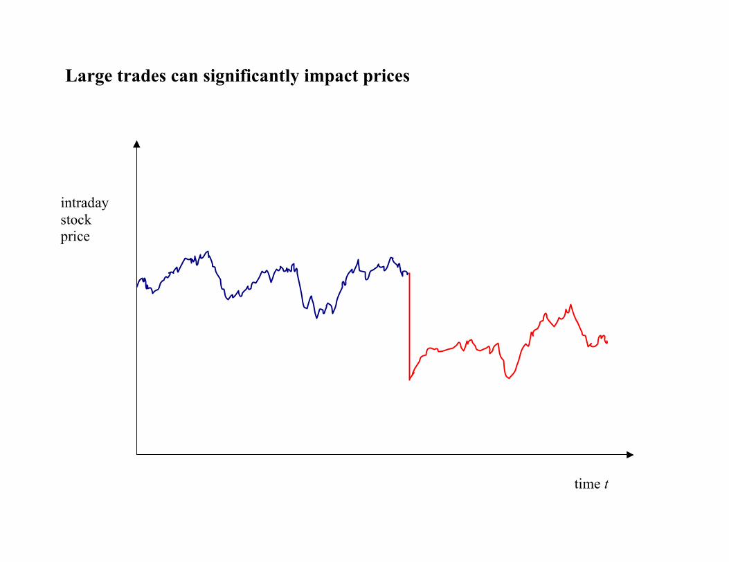
Large trades can significantly impact prices
time t
intraday
stock price
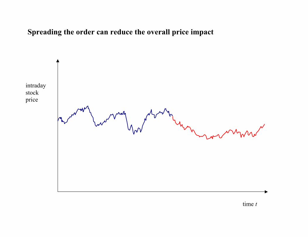
Spreading the order can reduce the overall price impact
time t
intraday
stock price
How to execute a single trade of selling X0 shares?
Interesting because:
• Liquidity/market impact risk in its purest form
– development of realistic market impact models
– checking viability of these models
– building block for more complex problems
• Relevant in applications
– real-world tests of new models
• Interesting mathematics
2
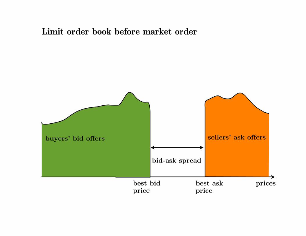
Limit order book before market order
buyers’ bid offers sellers’ ask offers
bid-ask spread
best bid price
best ask price
prices
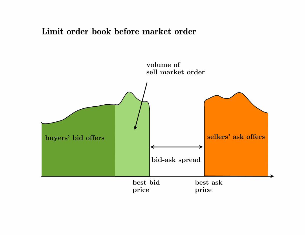
Limit order book before market order
buyers’ bid offers sellers’ ask offers
bid-ask spread
best bid price
best ask price
volume of sell market order
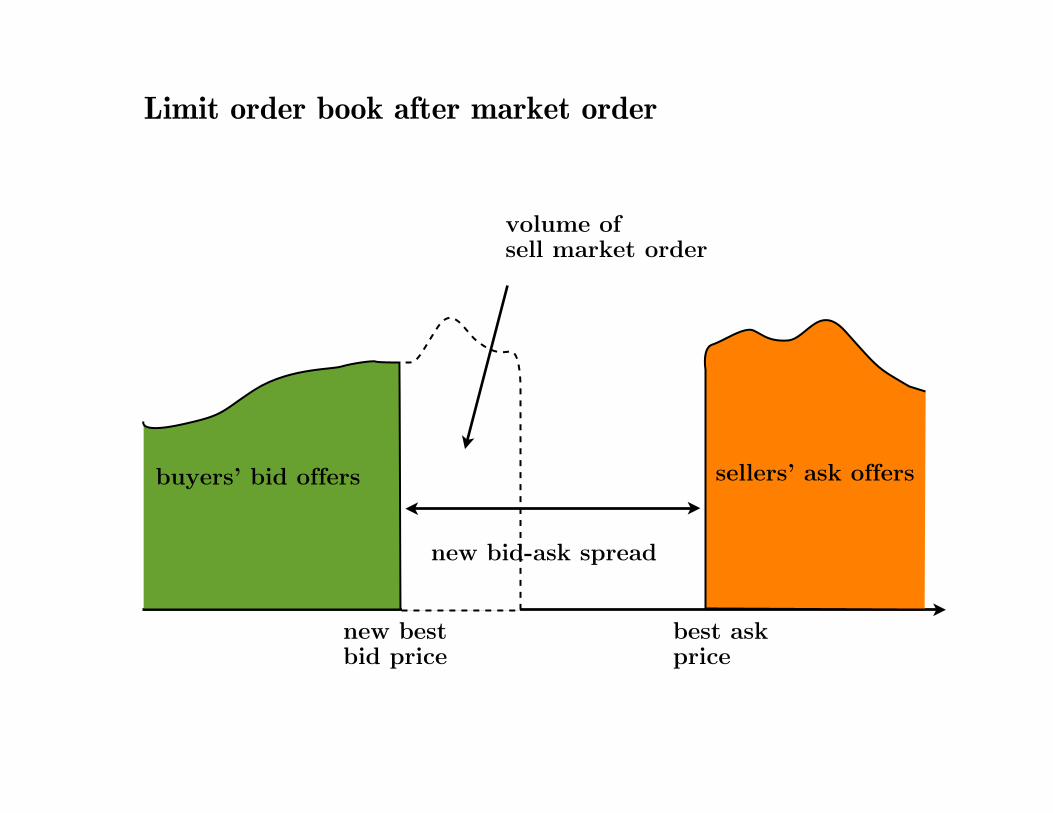
Limit order book after market order
buyers’ bid offers sellers’ ask offers
new bid-ask spread
new best bid price
best ask price
volume of sell market order
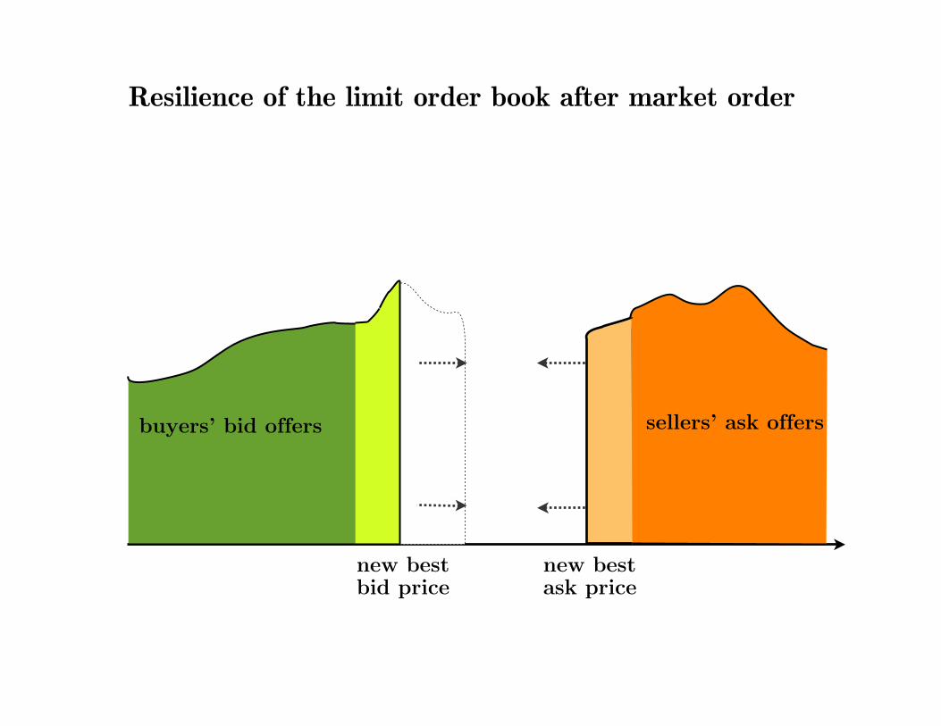
Resilience of the limit order book after market order
buyers’ bid offers sellers’ ask offers
new bestask price
new bestbid price
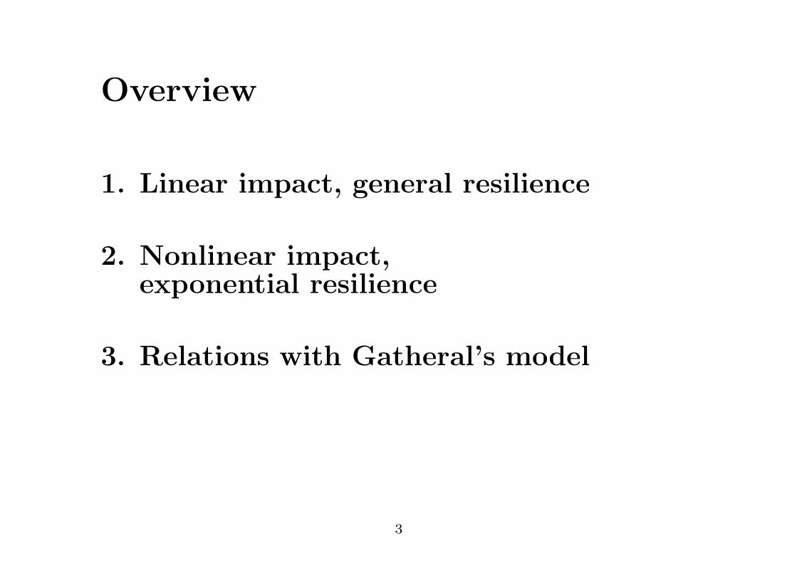
Overview
1. Linear impact, general resilience
2. Nonlinear impact,exponential resilience
3. Relations with Gatheral’s model
3
ReferencesA. Alfonsi, A. Fruth, and A.S.: Optimal execution strategies in limit
order books with general shape functions. To appear in QuantitativeFinance
A. Alfonsi, A. Fruth, and A.S.: Constrained portfolio liquidation in a
limit order book model. Banach Center Publ. 83, 9-25 (2008).
A. Alfonsi and A.S.: Optimal execution and absence of price
manipulations in limit order book models. Preprint 2009.
A. Alfonsi, A.S., and A. Slynko: Order book resilience, price
manipulations, and the positive portfolio problem. Preprint 2009.
J. Gatheral: No-Dynamic-Arbitrage and Market Impact. Preprint(2008).
A. Obizhaeva and J. Wang: Optimal Trading Strategy and
Supply/Demand Dynamics. Preprint (2005)
4
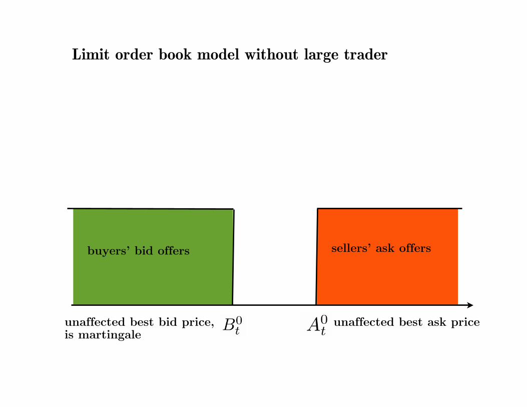
Limit order book model without large trader
unaffected best ask priceunaffected best bid price,is martingale
buyers’ bid offers sellers’ ask offers
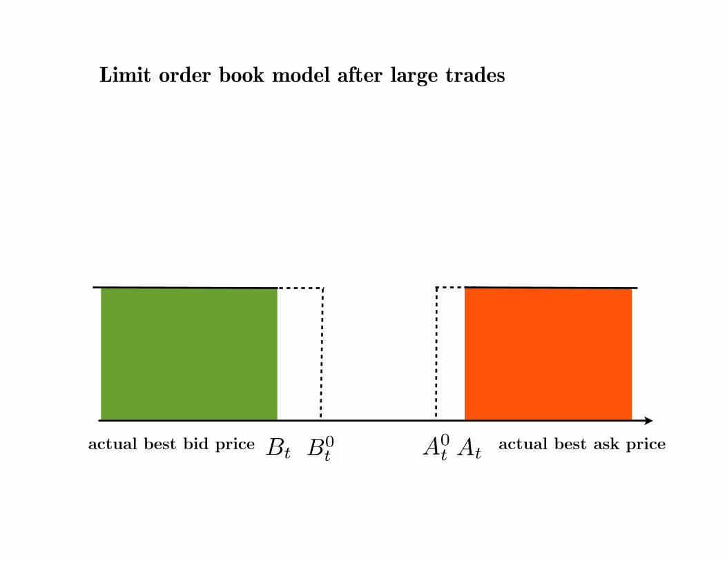
Limit order book model after large trades
actual best ask priceactual best bid price
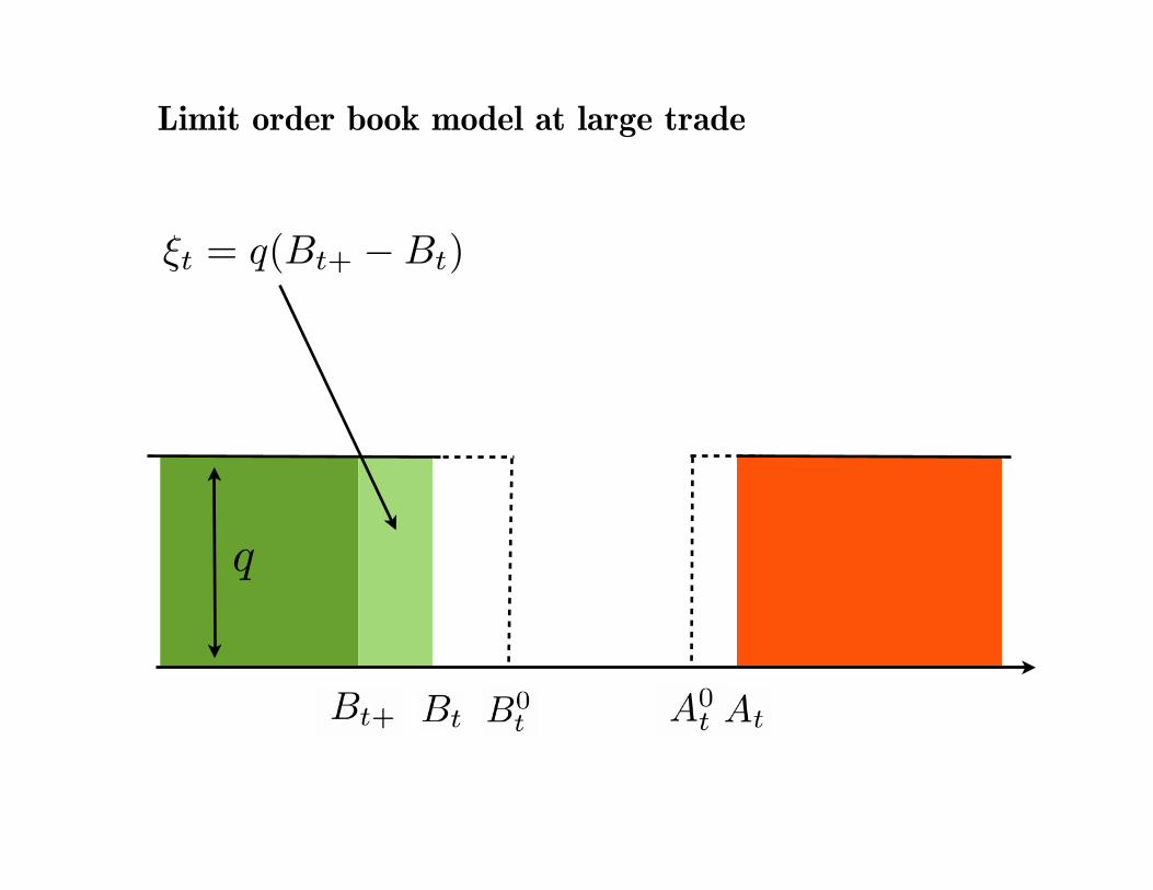
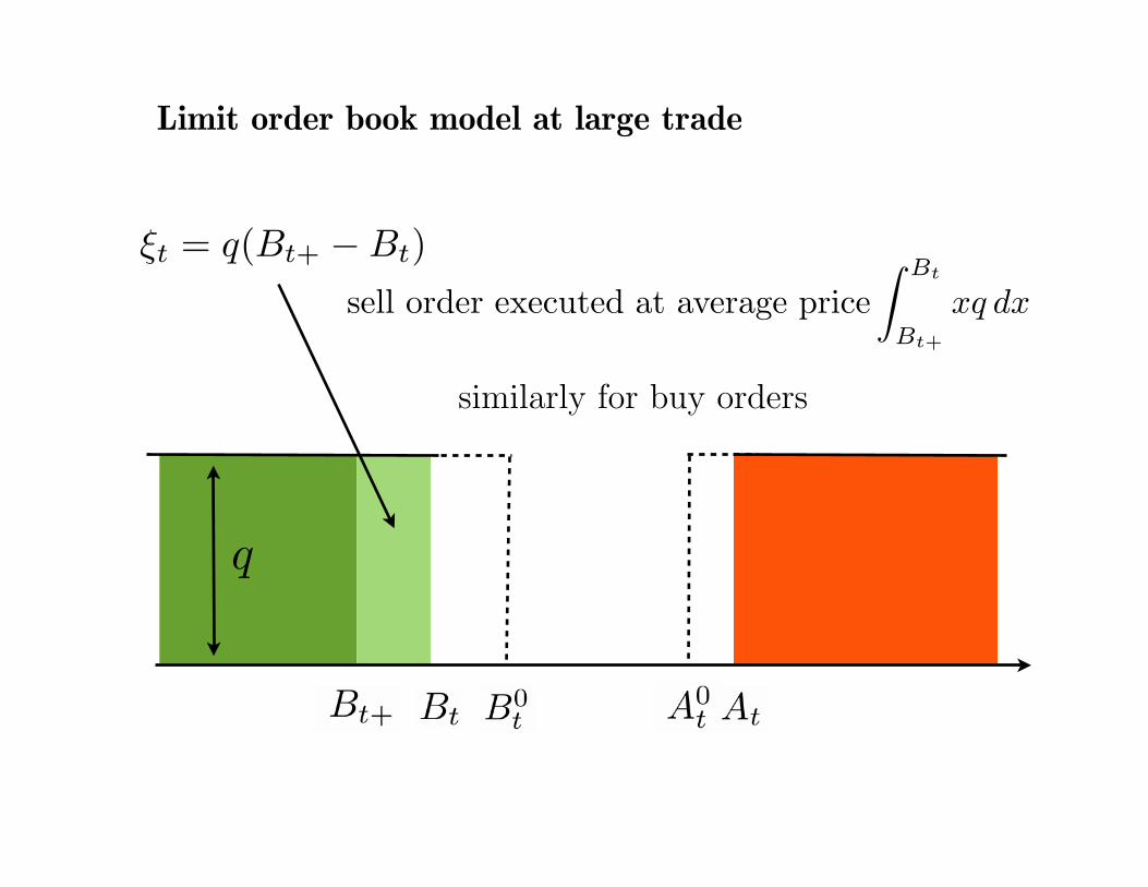
Limit order book model at large trade
B0t A0
t
Bt At
DAt DB
t
DAt+ DB
t+
Bt+ At+
Bt+!t At+!t
DAt+s DB
t+s
!t = q(Bt !Bt+)
!t
q · "(!t) + resilience of other trades
1
B0t A0
t
Bt At
DAt DB
t
DAt+ DB
t+
Bt+ At+
Bt+!t At+!t
DAt+s DB
t+s
!t = q(Bt+ !Bt)
!t
q · "(!t) + decay of previous trades
sell order executed at average price! Bt
Bt+
xq dx
similarly for buy orders
" : [0,"[# [0, 1], "(0) = 1, decreasing
1
Limit order book model at large trade
B0t A0
t
Bt At
DAt DB
t
DAt+ DB
t+
Bt+ At+
Bt+!t At+!t
DAt+s DB
t+s
!t = q(Bt !Bt+)
!t
q · "(!t) + resilience of other trades
1
similarly for buy orders
B0t A0
t
Bt At
DAt DB
t
DAt+ DB
t+
Bt+ At+
Bt+!t At+!t
DAt+s DB
t+s
!t = q(Bt !Bt+)
!t
q · "(!t) + decay of previous trades
sell order executed at average price! Bt
Bt+
xq dx
similarly for buy orders
" : [0,"[# [0, 1], "(0) = 1, decreasing
1
B0t A0
t
Bt At
DAt DB
t
DAt+ DB
t+
Bt+ At+
Bt+!t At+!t
DAt+s DB
t+s
!t = q(Bt+ !Bt)
!t
q · "(!t) + decay of previous trades
sell order executed at average price! Bt
Bt+
xq dx
similarly for buy orders
" : [0,"[# [0, 1], "(0) = 1, decreasing
1
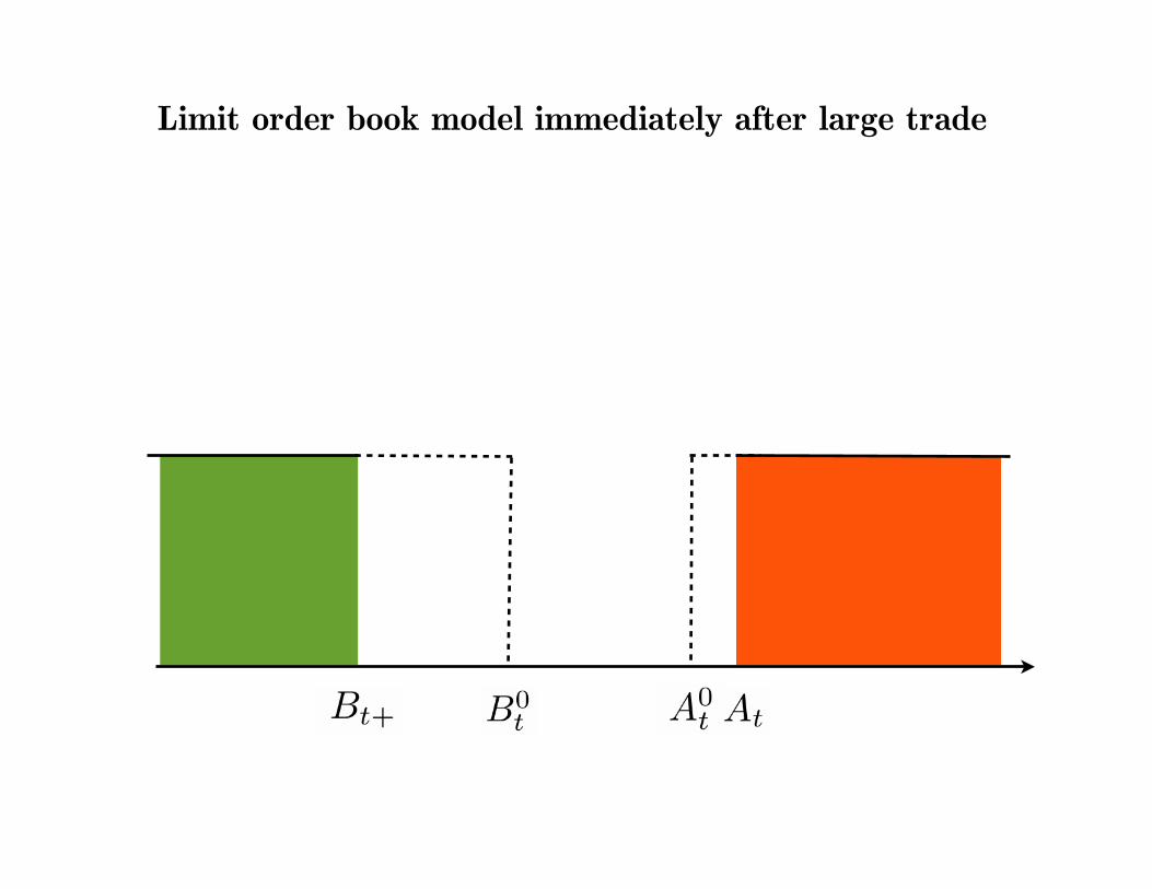
Limit order book model immediately after large trade
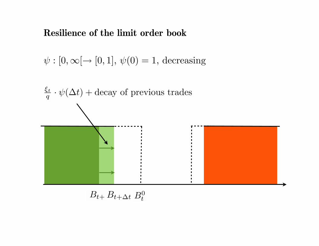
Resilience of the limit order book
B0t A0
t
Bt At
DAt DB
t
DAt+ DB
t+
Bt+ At+
Bt+!t At+!t
DAt+s DB
t+s
!t = q(Bt !Bt+)
!t
q · "(!t) + resilience of other trades
1
B0t A0
t
Bt At
DAt DB
t
DAt+ DB
t+
Bt+ At+
Bt+!t At+!t
DAt+s DB
t+s
!t = q(Bt !Bt+)
!t
q · "(!t) + decay of previous trades
liquidity costs = !tB0t !
! Bt
Bt+
qx dx
" : [0,"[# [0, 1], "(0) = 1, decreasing
1
B0t A0
t
Bt At
DAt DB
t
DAt+ DB
t+
Bt+ At+
Bt+!t At+!t
DAt+s DB
t+s
!t = q(Bt !Bt+)
!t
q · "(!t) + decay of previous trades
liquidity costs = !tB0t !
! Bt
Bt+
qx dx
" : [0,"[# [0, 1], "(0) = 1, decreasing
1

1. Linear impact, general resilienceStrategy:
N + 1 market orders: !n shares placed at time tn s.th.
a) 0 = t0 ! t1 ! · · · ! tN = T
(can also be stopping times)
b) !n is Ftn-measurable and bounded from below,
c) we haveN!
n=0
!n = X0
Sell order: !n < 0
Buy order: !n > 0
5
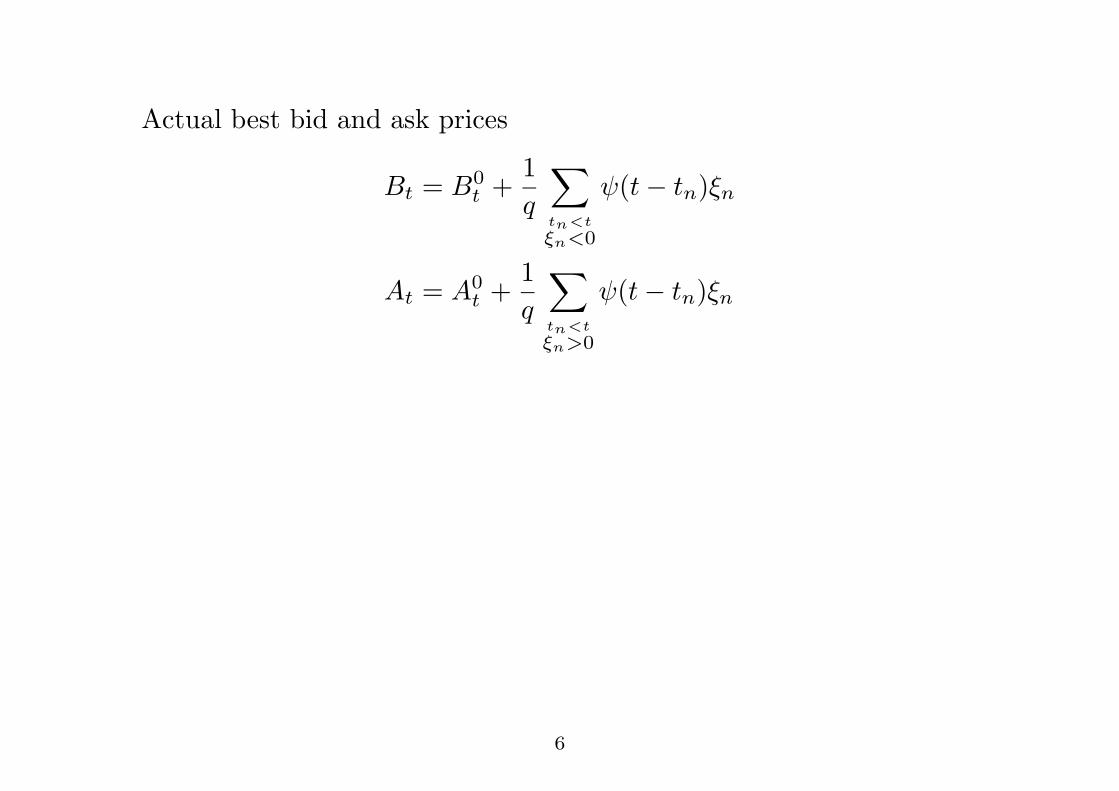
Actual best bid and ask prices
Bt = B0t +
1q
!
tn<t!n<0
"(t" tn)!n
At = A0t +
1q
!
tn<t!n>0
"(t" tn)!n
6
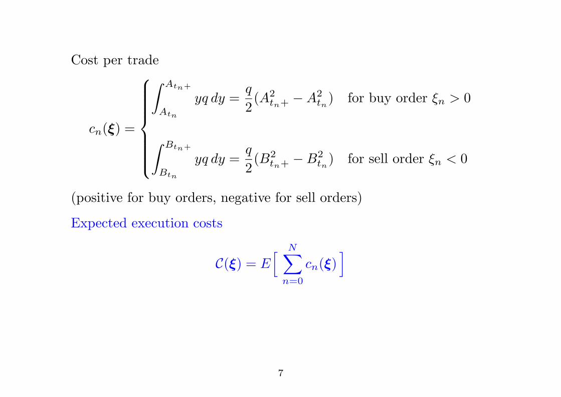
Cost per trade
cn(!) =
"######$
######%
& Atn+
Atn
yq dy =q
2(A2
tn+ "A2tn
) for buy order !n > 0
& Btn+
Btn
yq dy =q
2(B2
tn+ "B2tn
) for sell order !n < 0
(positive for buy orders, negative for sell orders)
Expected execution costs
C(!) = E' N!
n=0
cn(!)(
7
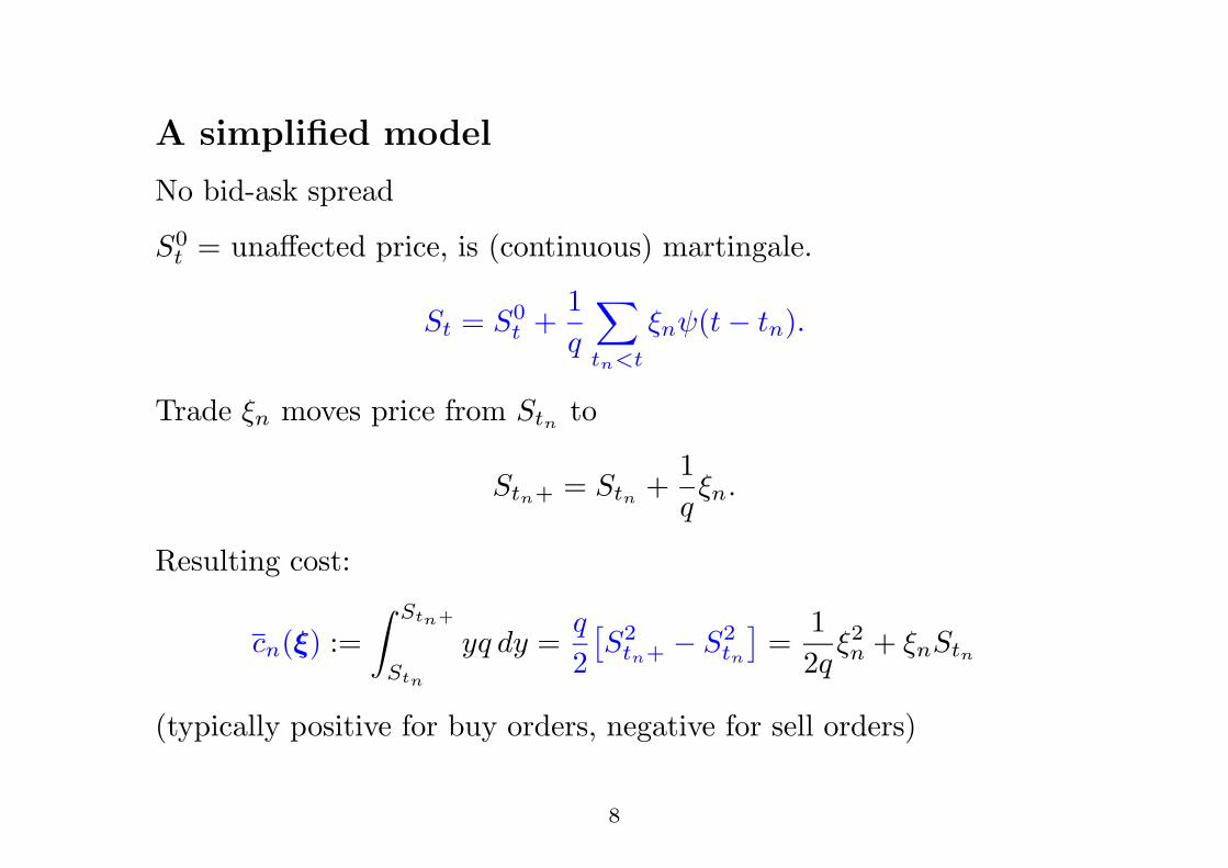
A simplified model
No bid-ask spread
S0t = una!ected price, is (continuous) martingale.
St = S0t +
1q
!
tn<t
!n"(t" tn).
Trade !n moves price from Stn to
Stn+ = Stn +1q!n.
Resulting cost:
cn(!) :=& Stn+
Stn
yq dy =q
2)S2
tn+ " S2tn
*=
12q
!2n + !nStn
(typically positive for buy orders, negative for sell orders)
8
Lemma 1. Suppose that S0 = A0. Then, for any strategy !,
cn(!) ! cn(!) with equality if !k # 0 for all k.
Thus: Enough to study the simplified model (as long as all trades !n
are positive)
9
Lemma 1. Suppose that S0 = A0. Then, for any strategy !,
cn(!) ! cn(!) with equality if !k # 0 for all k.
Thus: Enough to study the simplified model (as long as all trades !n
are positive)
9
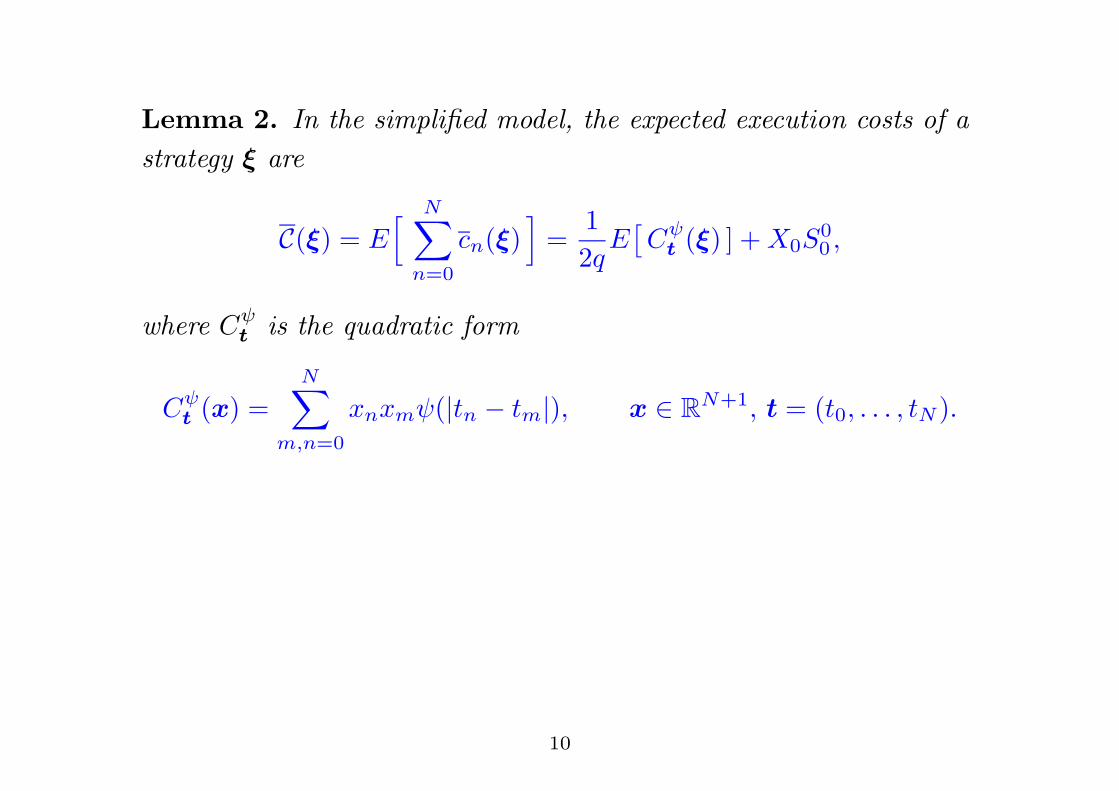
Lemma 2. In the simplified model, the expected execution costs of astrategy ! are
C(!) = E' N!
n=0
cn(!)(
=12q
E)C"
t (!) ] + X0S00 ,
where C"t is the quadratic form
C"t (x) =
N!
m,n=0
xnxm"(|tn " tm|), x $ RN+1, t = (t0, . . . , tN ).
10
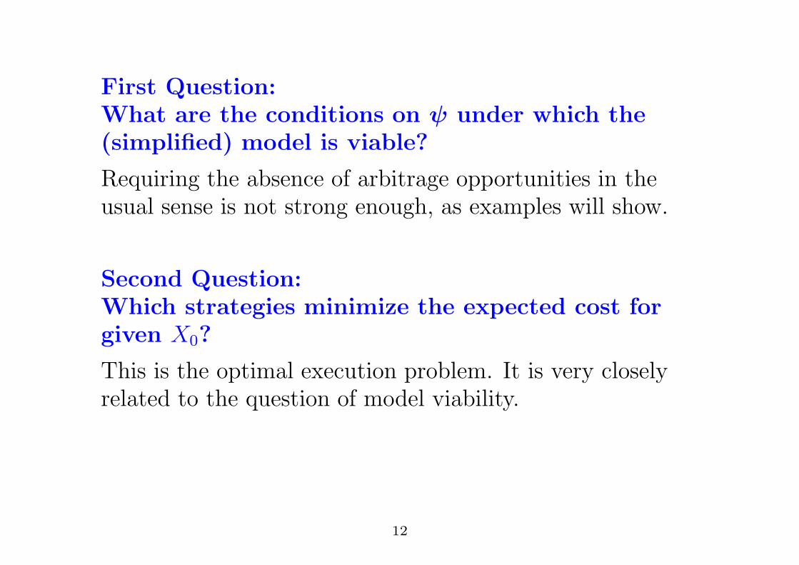
First Question:What are the conditions on " under which the(simplified) model is viable?
Requiring the absence of arbitrage opportunities in theusual sense is not strong enough, as examples will show.
Second Question:Which strategies minimize the expected cost forgiven X0?
This is the optimal execution problem. It is very closelyrelated to the question of model viability.
12
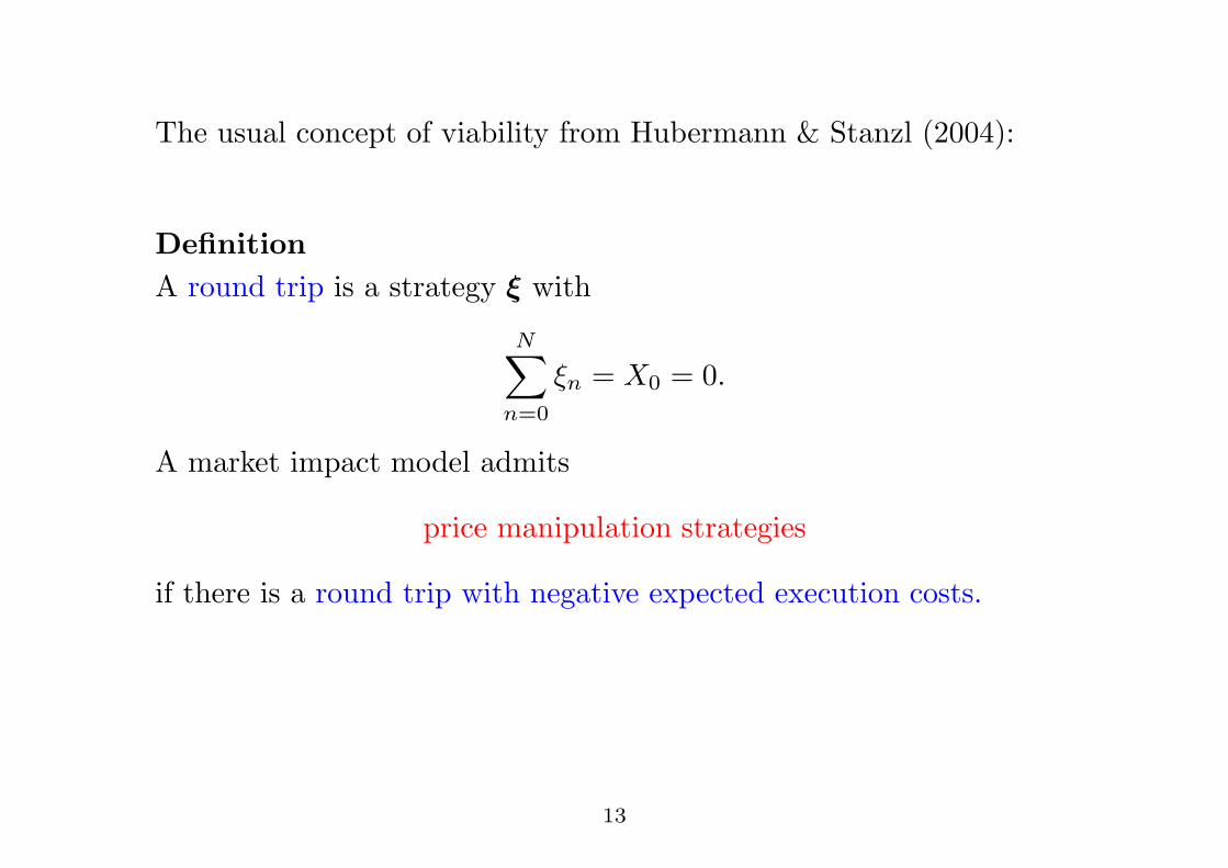
The usual concept of viability from Hubermann & Stanzl (2004):
DefinitionA round trip is a strategy ! with
N!
n=0
!n = X0 = 0.
A market impact model admits
price manipulation strategies
if there is a round trip with negative expected execution costs.
13
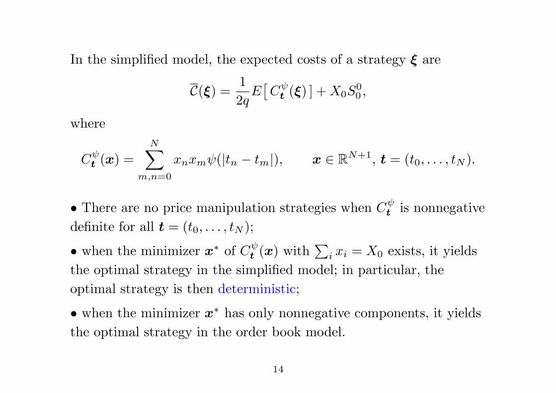
In the simplified model, the expected costs of a strategy ! are
C(!) =12q
E)C"
t (!) ] + X0S00 ,
where
C"t (x) =
N!
m,n=0
xnxm"(|tn " tm|), x $ RN+1, t = (t0, . . . , tN ).
• There are no price manipulation strategies when C"t is nonnegative
definite for all t = (t0, . . . , tN );
• when the minimizer x! of C"t (x) with
+i xi = X0 exists, it yields
the optimal strategy in the simplified model; in particular, theoptimal strategy is then deterministic;
• when the minimizer x! has only nonnegative components, it yieldsthe optimal strategy in the order book model.
14
Bochner’s theorem (1932):C"
t is always nonnegative definite (" is “positive definite”) if andonly if "(| · |) is the Fourier transform of a positive Borel measure µ
on R.
C"t is even strictly positive definite (" is “strictly positive definite”)
when the support of µ is not discrete.
15
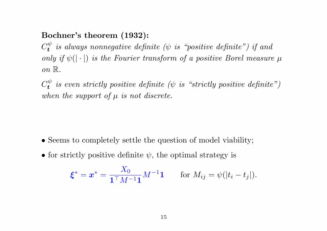
Bochner’s theorem (1932):C"
t is always nonnegative definite (" is “positive definite”) if andonly if "(| · |) is the Fourier transform of a positive Borel measure µ
on R.
C"t is even strictly positive definite (" is “strictly positive definite”)
when the support of µ is not discrete.
• Seems to completely settle the question of model viability;
• for strictly positive definite ", the optimal strategy is
!! = x! =X0
1"M#11M#11 for Mij = "(|ti " tj |).
15
Examples
Example 1: Exponential resilience[Obizhaeva & Wang (2005), Alfonsi, Fruth, S. (2008)]
For the exponential resilience function
"(t) = e##t,
"(| · |) is the Fourier transform of the positive measure
µ(dt) =1#
$
$2 + t2dt
Hence, " is strictly positive definite.
16
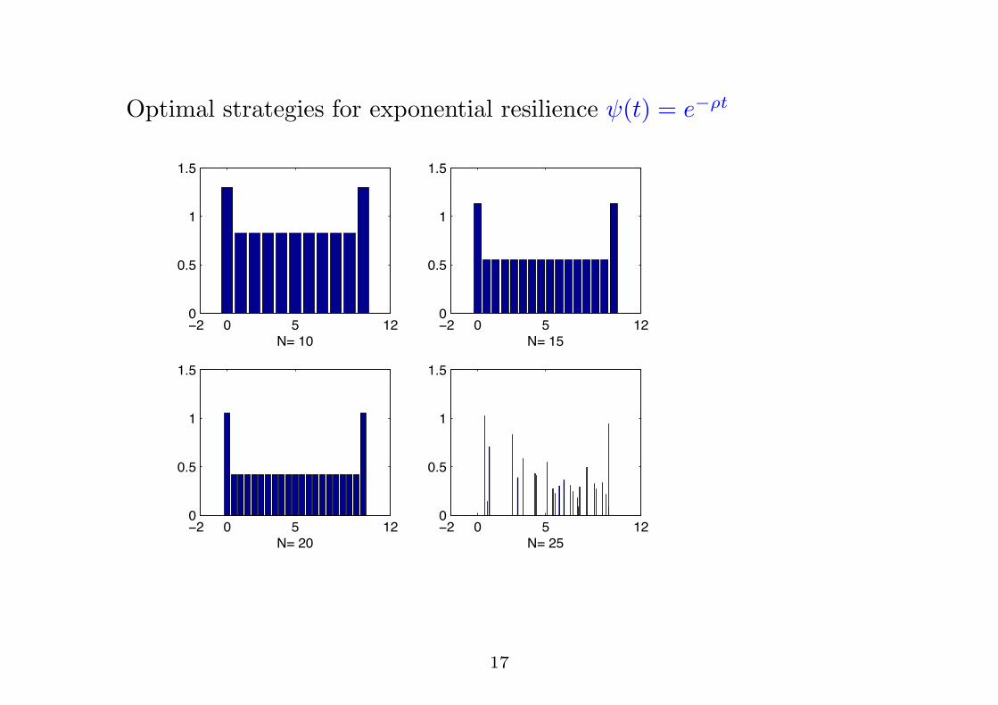
Optimal strategies for exponential resilience "(t) = e##t
!! " # $!"
"%#
$
$%#
&'($"
!! " # $!"
"%#
$
$%#
&'($#
!! " # $!"
"%#
$
$%#
&'(!"
!! " # $!"
"%#
$
$%#
&'(!#
17
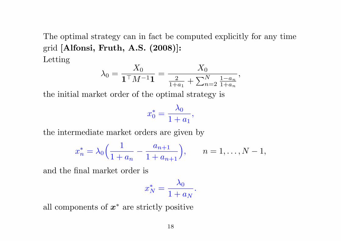
The optimal strategy can in fact be computed explicitly for any timegrid [Alfonsi, Fruth, A.S. (2008)]:Letting
%0 =X0
1"M#11=
X0
21+a1
++N
n=21#an1+an
,
the initial market order of the optimal strategy is
x!0 =%0
1 + a1,
the intermediate market orders are given by
x!n = %0
, 11 + an
" an+1
1 + an+1
-, n = 1, . . . , N " 1,
and the final market order is
x!N =%0
1 + aN.
all components of x! are strictly positive
18
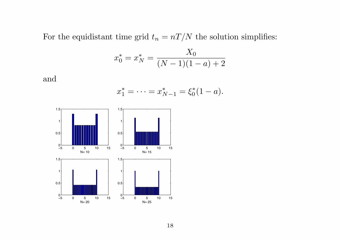
For the equidistant time grid tn = nT/N the solution simplifies:
x!0 = x!N =X0
(N " 1)(1" a) + 2
andx!1 = · · · = x!N#1 = !!0(1" a).
!! " ! #" #!"
"$!
#
#$!
%&'#"
!! " ! #" #!"
"$!
#
#$!
%&'#!
!! " ! #" #!"
"$!
#
#$!
%&'("
!! " ! #" #!"
"$!
#
#$!
%&'(!
18
The symmetry of the optimal strategy is a general fact:
Proposition 3. Suppose that " is strictly positive definite and thatthe time grid is symmetric, i.e.,
ti = tN " tN#i for all i,
then the optimal strategy is reversible, i.e.,
x!ti= x!tN!i
for all i.
19
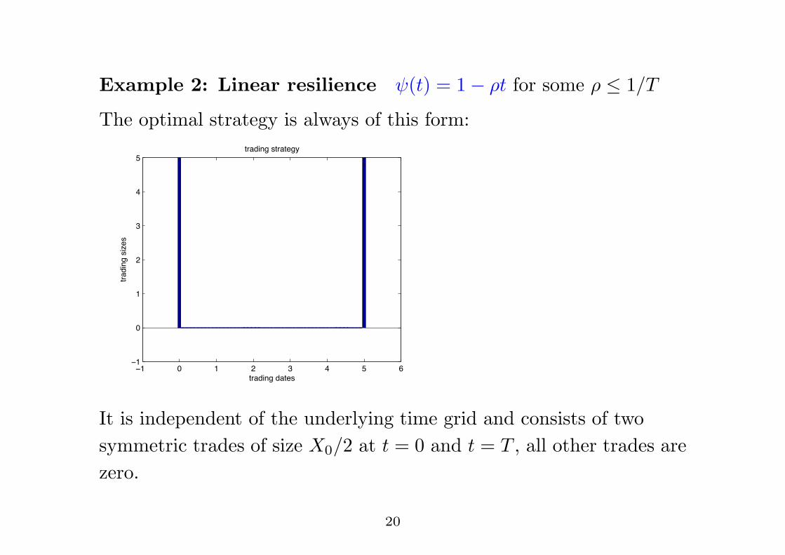
Example 2: Linear resilience "(t) = 1" $t for some $ ! 1/T
The optimal strategy is always of this form:
!! " ! # $ % & '!!
"
!
#
$
%
&
()*+,-./+*(01
()*+,-./1,201
()*+,-./1()*(0.3
It is independent of the underlying time grid and consists of twosymmetric trades of size X0/2 at t = 0 and t = T , all other trades arezero.
20
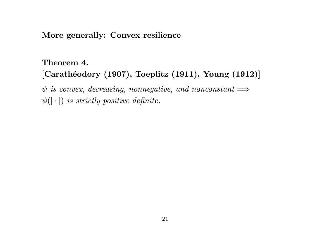
More generally: Convex resilience
Theorem 4.[Caratheodory (1907), Toeplitz (1911), Young (1912)]
" is convex, decreasing, nonnegative, and nonconstant =%"(| · |) is strictly positive definite.
21
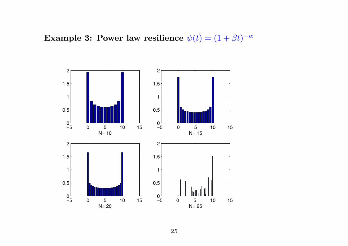
Example 3: Power law resilience "(t) = (1 + &t)#$
!! " ! #" #!"
"$!
#
#$!
%
&'(#"
!! " ! #" #!"
"$!
#
#$!
%
&'(#!
!! " ! #" #!"
"$!
#
#$!
%
&'(%"
!! "( !( #" #!"
"$!
#
#$!
%
&'(%!
25
Example 4: Trigonometric resilienceThe function
cos $x
is the Fourier transform of the positive finite measure
µ =12('## + '#)
Since it is not strictly positive definite, we take
"(t) = (1" () cos $t + (e#t for some $ ! #
2T.
26
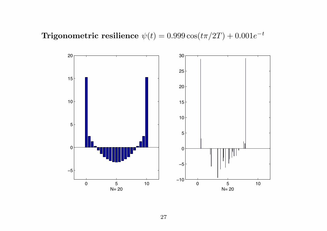
Trigonometric resilience "(t) = 0.999 cos(t#/2T ) + 0.001e#t
! " #!
!"
!
"
#!
#"
$!
%&'$!
! " #!!#!
!"
!
"
#!
#"
$!
$"
(!
%&'$!
27
Example 5: Gaussian resilience
The Gaussian resilience function
"(t) = e#t2
is its own Fourier transform (modulo constants). The correspondingquadratic form is hence positive definite.
Nevertheless.....
28
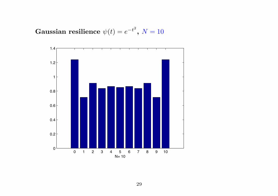
Gaussian resilience "(t) = e#t2 , N = 10
0 1 2 3 4 5 6 7 8 9 100
0.2
0.4
0.6
0.8
1
1.2
1.4
N= 10
29
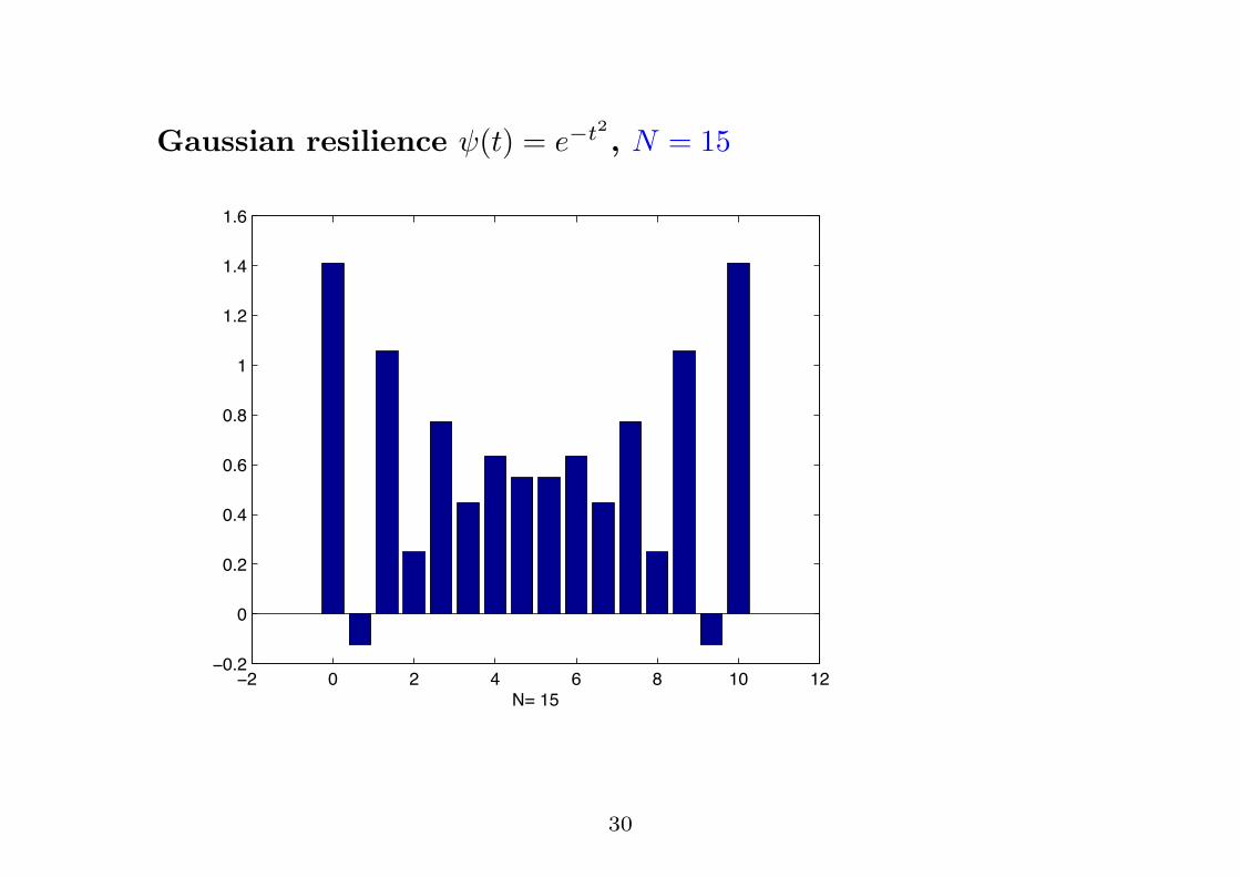
Gaussian resilience "(t) = e#t2 , N = 15
!! " ! # $ % &" &!!"'!
"
"'!
"'#
"'$
"'%
&
&'!
&'#
&'$
()*&+
30
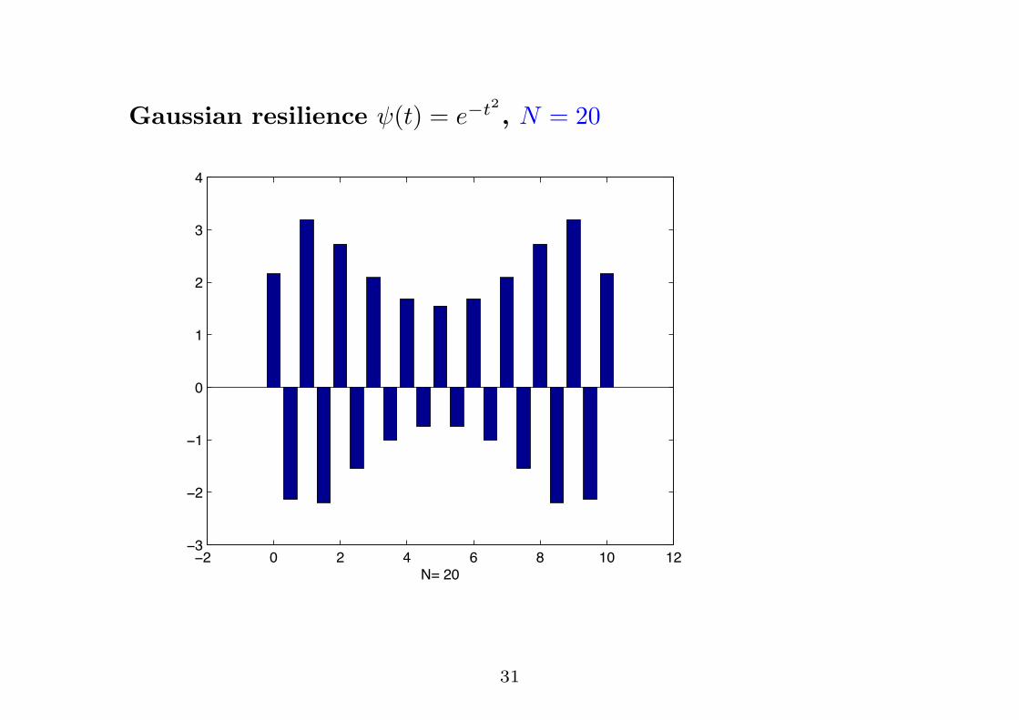
Gaussian resilience "(t) = e#t2 , N = 20
!! " ! # $ % &" &!!'
!!
!&
"
&
!
'
#
()*!"
31
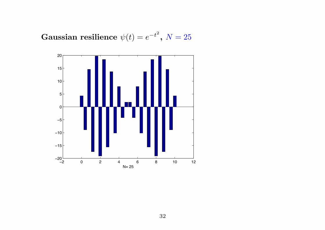
Gaussian resilience "(t) = e#t2 , N = 25
!! " ! # $ % &" &!!!"
!&'
!&"
!'
"
'
&"
&'
!"
()*!'
32
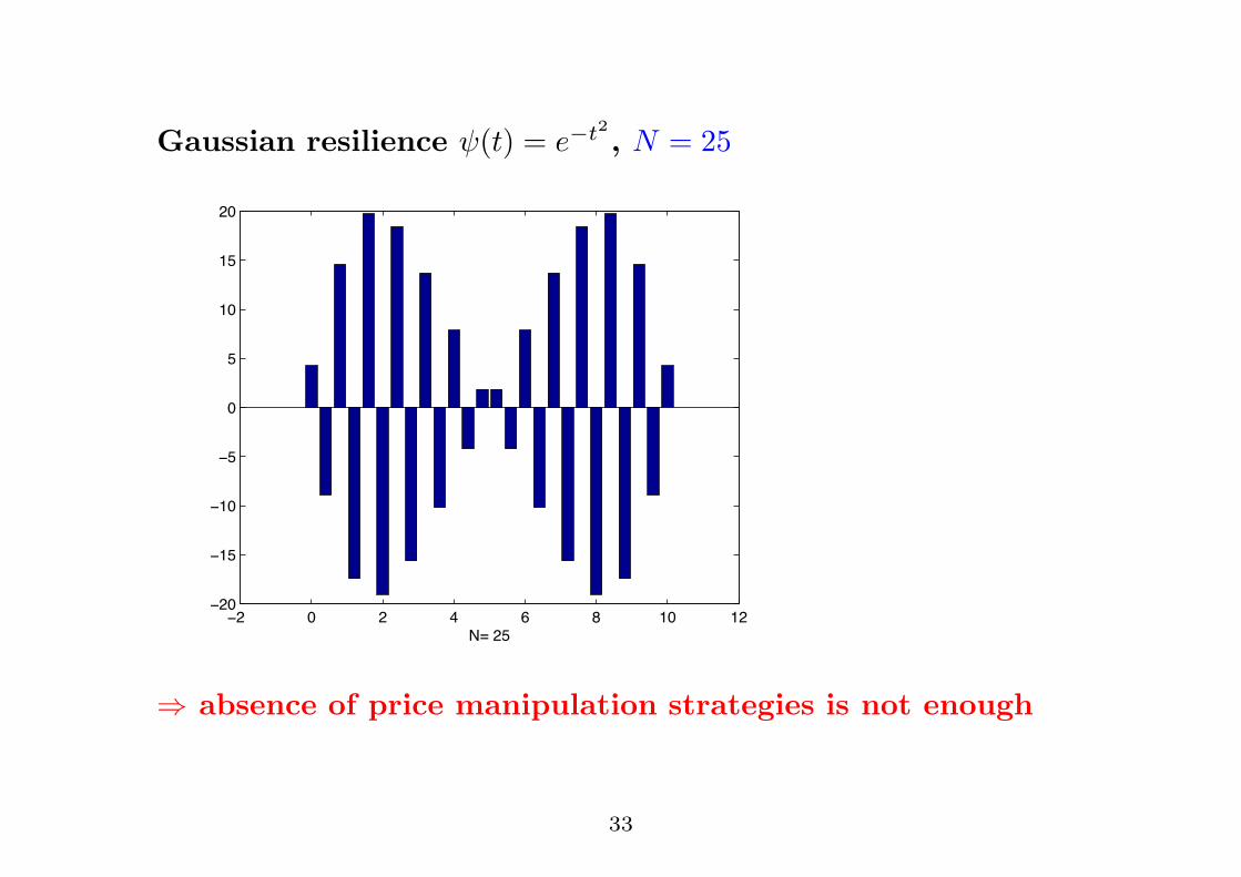
Gaussian resilience "(t) = e#t2 , N = 25
!! " ! # $ % &" &!!!"
!&'
!&"
!'
"
'
&"
&'
!"
()*!'
% absence of price manipulation strategies is not enough
33
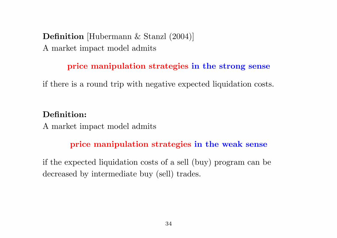
Definition [Hubermann & Stanzl (2004)]A market impact model admits
price manipulation strategies in the strong sense
if there is a round trip with negative expected liquidation costs.
Definition:A market impact model admits
price manipulation strategies in the weak sense
if the expected liquidation costs of a sell (buy) program can bedecreased by intermediate buy (sell) trades.
34
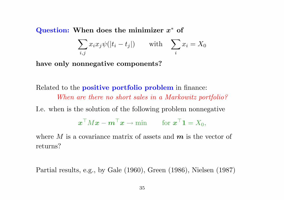
Question: When does the minimizer x! of!
i,j
xixj"(|ti " tj |) with!
i
xi = X0
have only nonnegative components?
Related to the positive portfolio problem in finance:When are there no short sales in a Markowitz portfolio?
I.e. when is the solution of the following problem nonnegative
x"Mx"m"x& min for x"1 = X0,
where M is a covariance matrix of assets and m is the vector ofreturns?
Partial results, e.g., by Gale (1960), Green (1986), Nielsen (1987)
35
Proposition 5. [Alfonsi, A.S., Slynko (2009)]When " is strictly positive definite and trading times are equidistant,then
x!0 > 0 and x!N > 0.
Proof relies on Trench algorithm for inverting the Toeplitz matrix
Mij = "(|i" j|/N), i, j = 0, . . . , N
36
Theorem 6. [Alfonsi, A.S., Slynko (2009)]
• If " is convex then all components of x! are nonnegative.
• If " is strictly convex, then all components are strictly positive.
• Conversely, x! has negative components as soon as, e.g., " isstrictly concave in a neighborhood of 0.
37
Qualitative properties of optimal strategies?
41
Qualitative properties of optimal strategies?
Proposition 8. [Alfonsi, A.S., Slynko (2009)]When " is convex and nonconstant, the optimal x! satisfies
x!0 # x!1 and x!N#1 ! x!N
41
Proof: Equating the first and second equations in Mx! = %01 givesN!
j=0
x!j"(tj) =N!
j=0
x!j"(|tj " t1|).
Thus,
x!0 " x!1 =N!
j=0, j $=1
x!j"(|tj " t1|)"N!
j=1
x!j"(tj)
= x!0"(t1)" x!1"(t1) +N!
j=2
x!j)"(tj " t1)" "(tj)
*
# (x!0 " x!1)"(t1),
by convexity of ". Therefore
(x0 " x1)(1" "(t1)) # 0
42
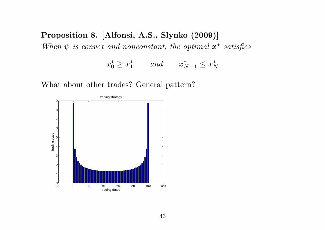
Proposition 8. [Alfonsi, A.S., Slynko (2009)]When " is convex and nonconstant, the optimal x! satisfies
x!0 # x!1 and x!N#1 ! x!N
What about other trades? General pattern?
!!" " !" #" $" %" &"" &!""
&
!
'
#
(
$
)
%
*
+,-./012.-+34
+,-./0124/534
+,-./0124+,-+316
43
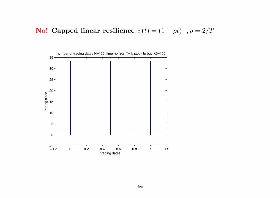
No! Capped linear resilience "(t) = (1" $t)+, $ = 2/T
!!"# ! !"# !"$ !"% !"& ' '"#!(
!
(
'!
'(
#!
#(
)!
)(
*+,-./01-,*23
*+,-./013.423
1/5672+1891*+,-./01-,*231:;'!!<1*.621=8+.48/1>;'<13*8?@1*8175A1B!;'!!
44
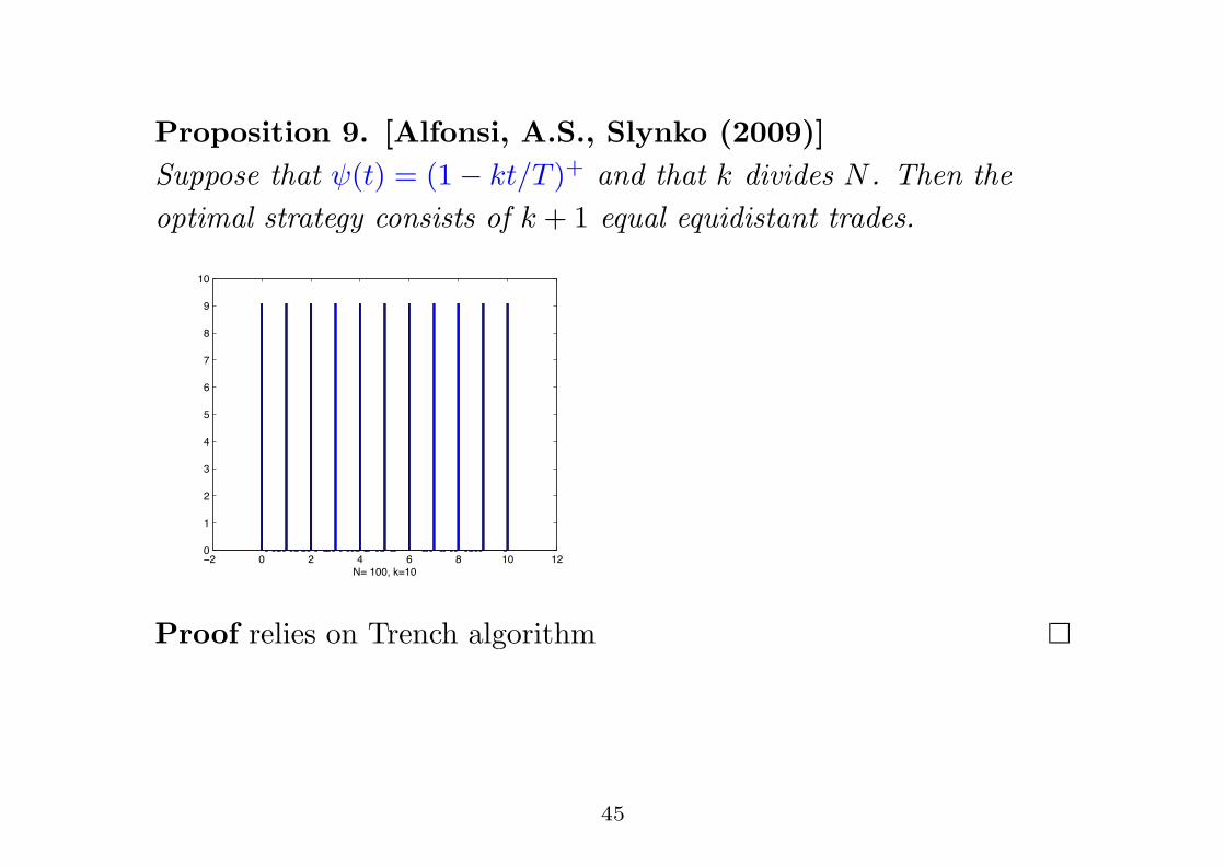
Proposition 9. [Alfonsi, A.S., Slynko (2009)]Suppose that "(t) = (1" kt/T )+ and that k divides N . Then theoptimal strategy consists of k + 1 equal equidistant trades.
!! " ! # $ % &" &!"
&
!
'
#
(
$
)
%
*
&"
+,-&"".-/,&"
Proof relies on Trench algorithm
45
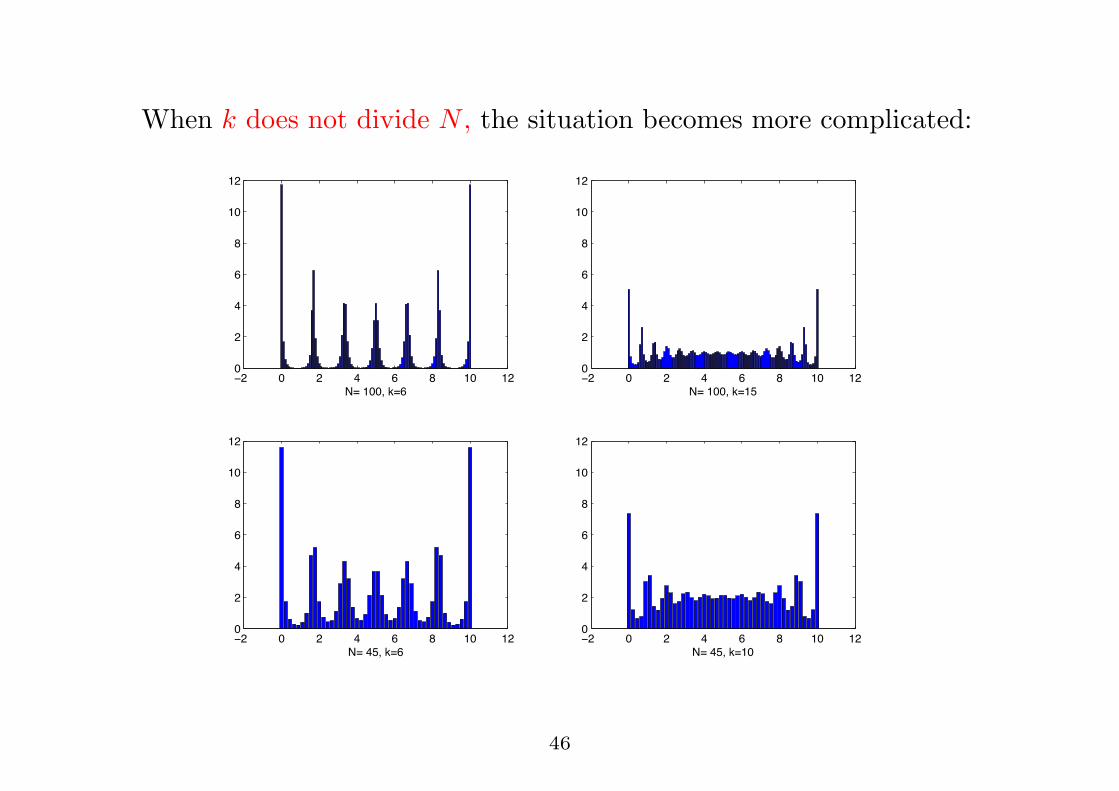
When k does not divide N , the situation becomes more complicated:
!! " ! # $ % &" &!"
!
#
$
%
&"
&!
'()&""*)+($
!! " ! # $ % &" &!"
!
#
$
%
&"
&!
'()&""*)+(&,
!! " ! # $ % &" &!"
!
#
$
%
&"
&!
'()#,*)+($
!! " ! # $ % &" &!"
!
#
$
%
&"
&!
'()#,*)+(&"
46
1. Linear impact, general resilience
2. Nonlinear impact,exponential resilience
47
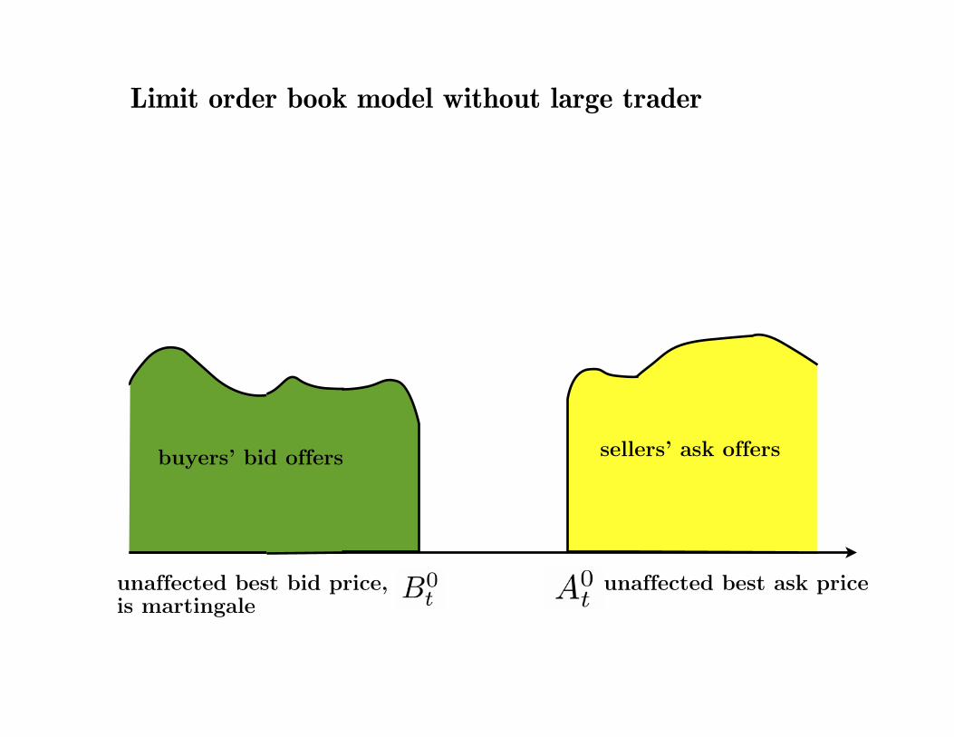
Limit order book model without large trader
buyers’ bid offers sellers’ ask offers
unaffected best ask priceunaffected best bid price,is martingale
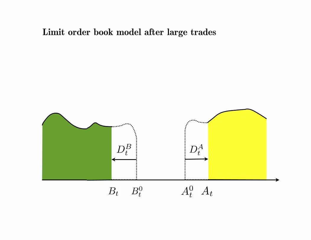
Limit order book model after large trades
Limit order book model at large trade
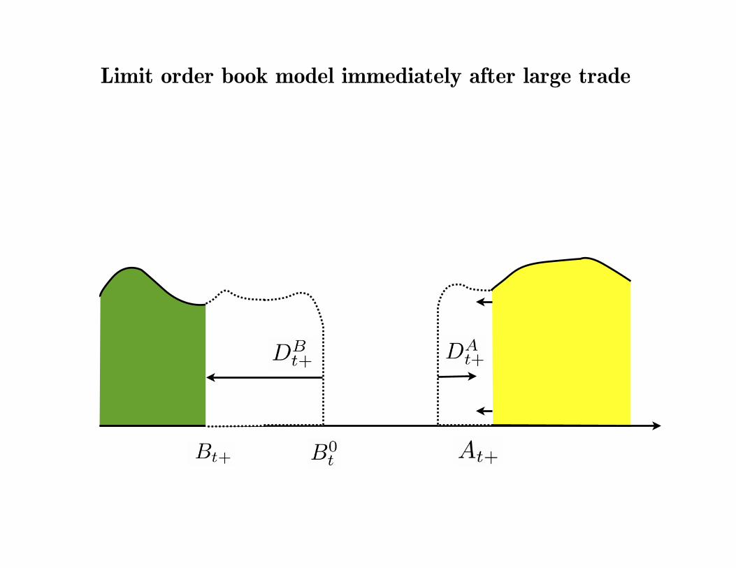
Limit order book model immediately after large trade
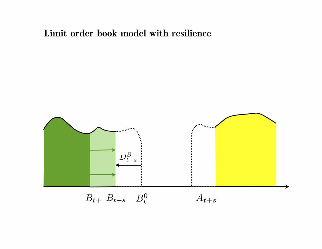
Limit order book model with resilience
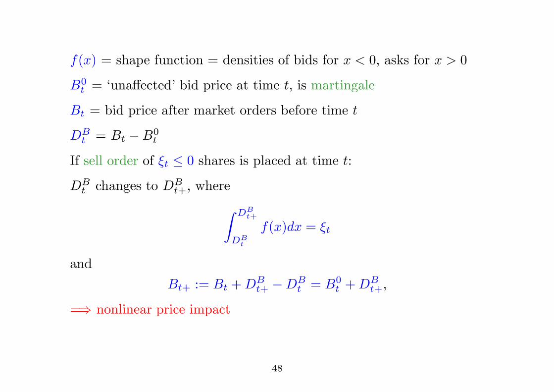
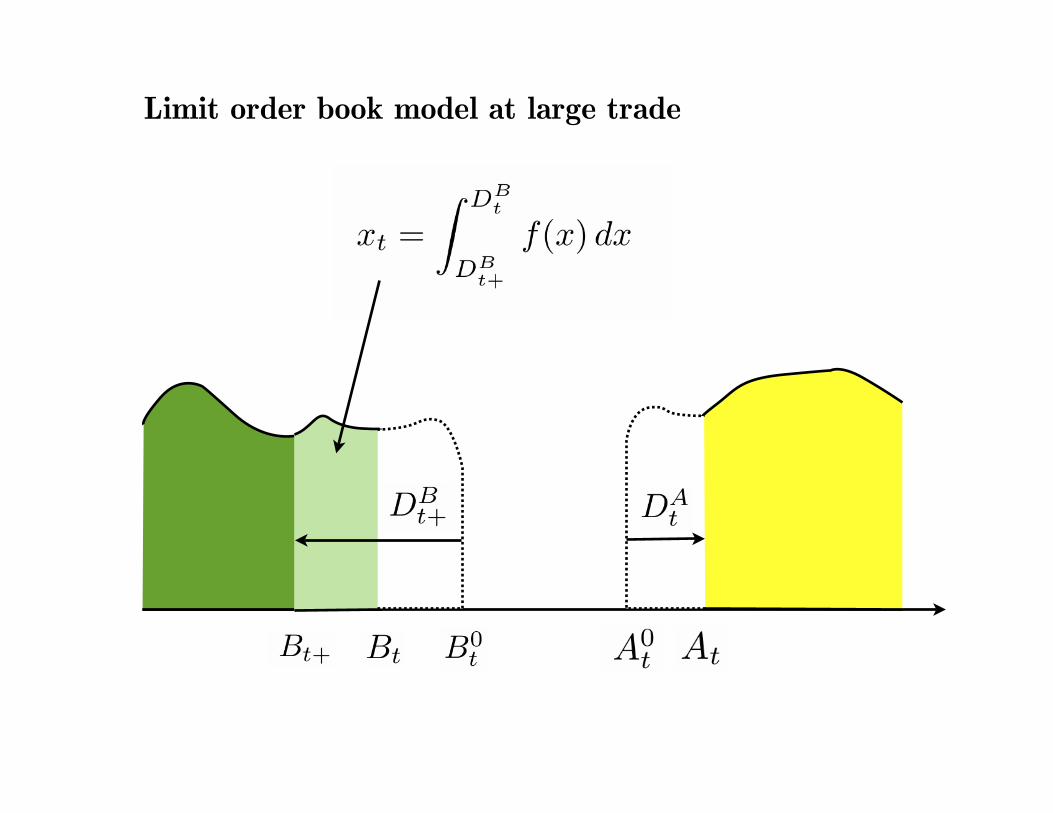
f(x) = shape function = densities of bids for x < 0, asks for x > 0
B0t = ‘una!ected’ bid price at time t, is martingale
Bt = bid price after market orders before time t
DBt = Bt "B0
t
If sell order of !t ! 0 shares is placed at time t:
DBt changes to DB
t+, where
& DBt+
DBt
f(x)dx = !t
andBt+ := Bt + DB
t+ "DBt = B0
t + DBt+,
=% nonlinear price impact
48
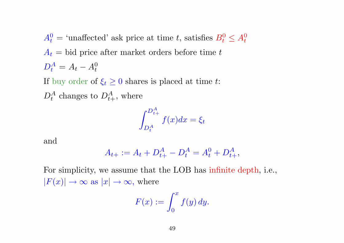
A0t = ‘una!ected’ ask price at time t, satisfies B0
t ! A0t
At = bid price after market orders before time t
DAt = At "A0
t
If buy order of !t # 0 shares is placed at time t:
DAt changes to DA
t+, where& DA
t+
DAt
f(x)dx = !t
andAt+ := At + DA
t+ "DAt = A0
t + DAt+,
For simplicity, we assume that the LOB has infinite depth, i.e.,|F (x)|&' as |x|&', where
F (x) :=& x
0f(y) dy.
49
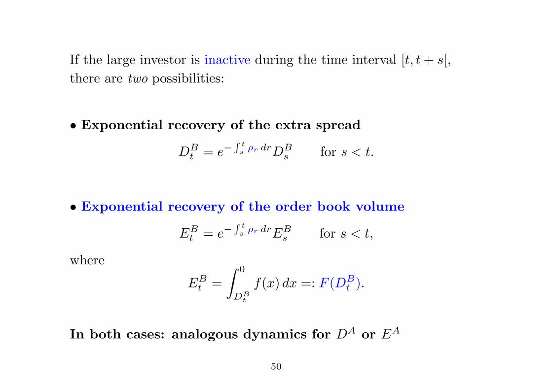
If the large investor is inactive during the time interval [t, t + s[,there are two possibilities:
• Exponential recovery of the extra spread
DBt = e#
! ts #r drDB
s for s < t.
• Exponential recovery of the order book volume
EBt = e#
! ts #r drEB
s for s < t,
where
EBt =
& 0
DBt
f(x) dx =: F (DBt ).
In both cases: analogous dynamics for DA or EA
50
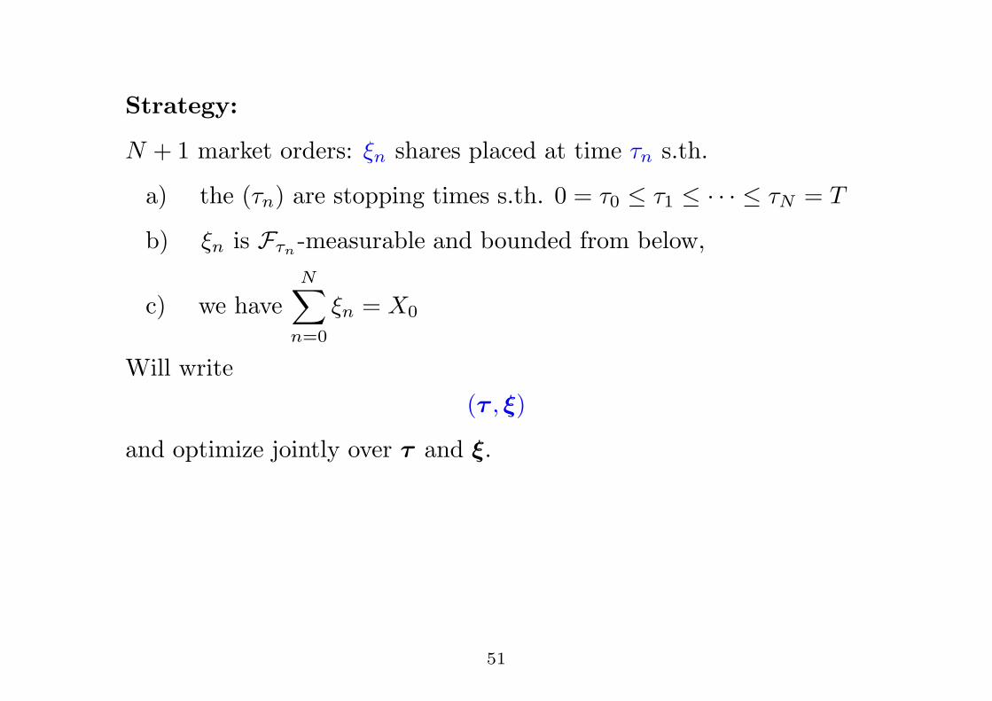
Strategy:
N + 1 market orders: !n shares placed at time )n s.th.
a) the ()n) are stopping times s.th. 0 = )0 ! )1 ! · · · ! )N = T
b) !n is F%n-measurable and bounded from below,
c) we haveN!
n=0
!n = X0
Will write(# , !)
and optimize jointly over # and !.
51
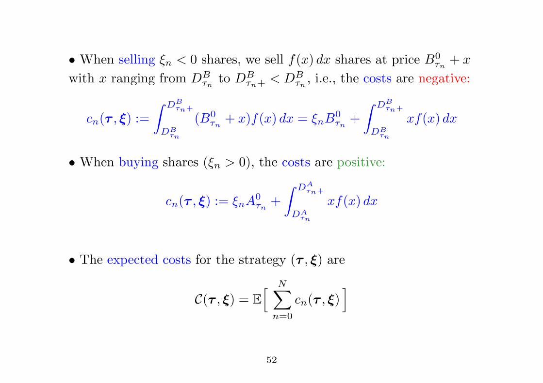
• When selling !n < 0 shares, we sell f(x) dx shares at price B0%n
+ x
with x ranging from DB%n
to DB%n+ < DB
%n, i.e., the costs are negative:
cn(# , !) :=& DB
!n+
DB!n
(B0%n
+ x)f(x) dx = !nB0%n
+& DB
!n+
DB!n
xf(x) dx
• When buying shares (!n > 0), the costs are positive:
cn(# , !) := !nA0%n
+& DA
!n+
DA!n
xf(x) dx
• The expected costs for the strategy (# , !) are
C(# , !) = E' N!
n=0
cn(# , !)(
52
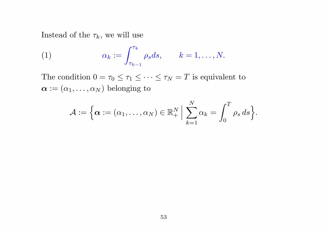
Instead of the )k, we will use
(1) *k :=& %k
%k!1
$sds, k = 1, . . . , N.
The condition 0 = )0 ! )1 ! · · · ! )N = T is equivalent to$ := (*1, . . . ,*N ) belonging to
A :=.$ := (*1, . . . ,*N ) $ RN
+
///N!
k=1
*k =& T
0$s ds
0.
53
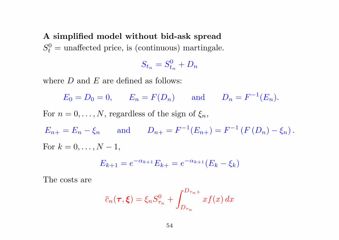
A simplified model without bid-ask spreadS0
t = una!ected price, is (continuous) martingale.
Stn = S0tn
+ Dn
where D and E are defined as follows:
E0 = D0 = 0, En = F (Dn) and Dn = F#1(En).
For n = 0, . . . , N , regardless of the sign of !n,
En+ = En " !n and Dn+ = F#1(En+) = F#1 (F (Dn)" !n) .
For k = 0, . . . , N " 1,
Ek+1 = e#$k+1Ek+ = e#$k+1(Ek " !k)
The costs are
cn(# , !) = !nS0%n
+& D!n+
D!n
xf(x) dx
54
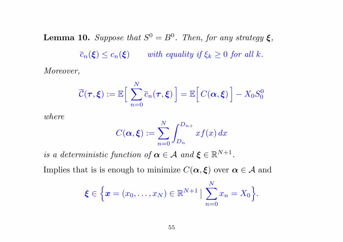
Lemma 10. Suppose that S0 = B0. Then, for any strategy !,
cn(!) ! cn(!) with equality if !k # 0 for all k.
Moreover,
C(# , !) := E' N!
n=0
cn(# , !)(
= E'C($, !)
("X0S
00
where
C($, !) :=N!
n=0
& Dn+
Dn
xf(x) dx
is a deterministic function of $ $ A and ! $ RN+1.
Implies that is is enough to minimize C($, !) over $ $ A and
! $.x = (x0, . . . , xN ) $ RN+1
//N!
n=0
xn = X0
0.
55
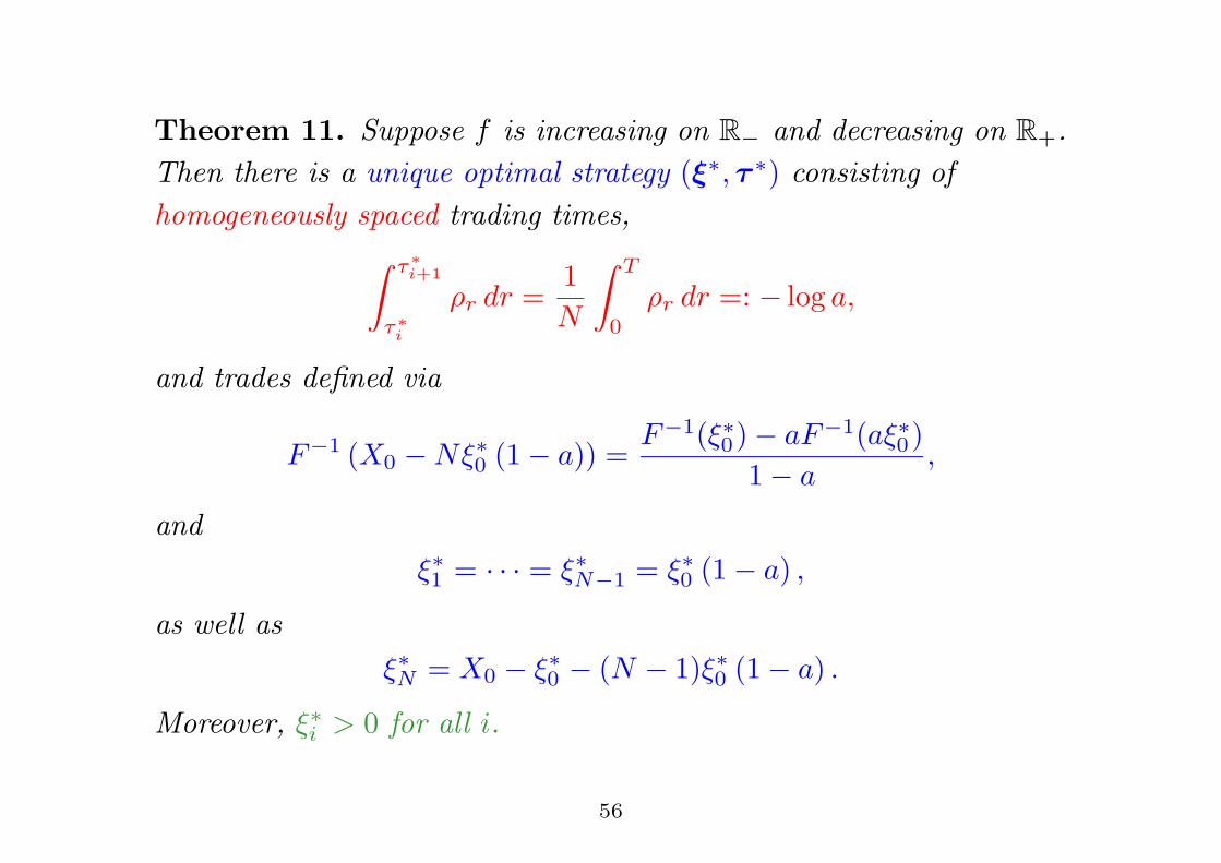
Theorem 11. Suppose f is increasing on R# and decreasing on R+.Then there is a unique optimal strategy (!!, # !) consisting ofhomogeneously spaced trading times,
& %"i+1
%"i
$r dr =1N
& T
0$r dr =: " log a,
and trades defined via
F#1 (X0 "N!!0 (1" a)) =F#1(!!0)" aF#1(a!!0)
1" a,
and!!1 = · · · = !!N#1 = !!0 (1" a) ,
as well as!!N = X0 " !!0 " (N " 1)!!0 (1" a) .
Moreover, !!i > 0 for all i.
56
Taking X0 ( 0 yields:
Corollary 12. Both the original and simplified models admit neitherstrong nor weak price manipulation strategies.
57
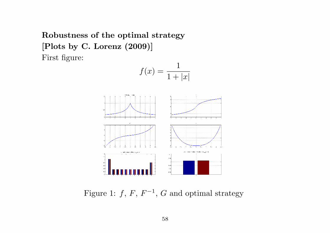
Robustness of the optimal strategy[Plots by C. Lorenz (2009)]First figure:
f(x) =1
1 + |x|
Figure 1: f , F , F#1, G and optimal strategy
58
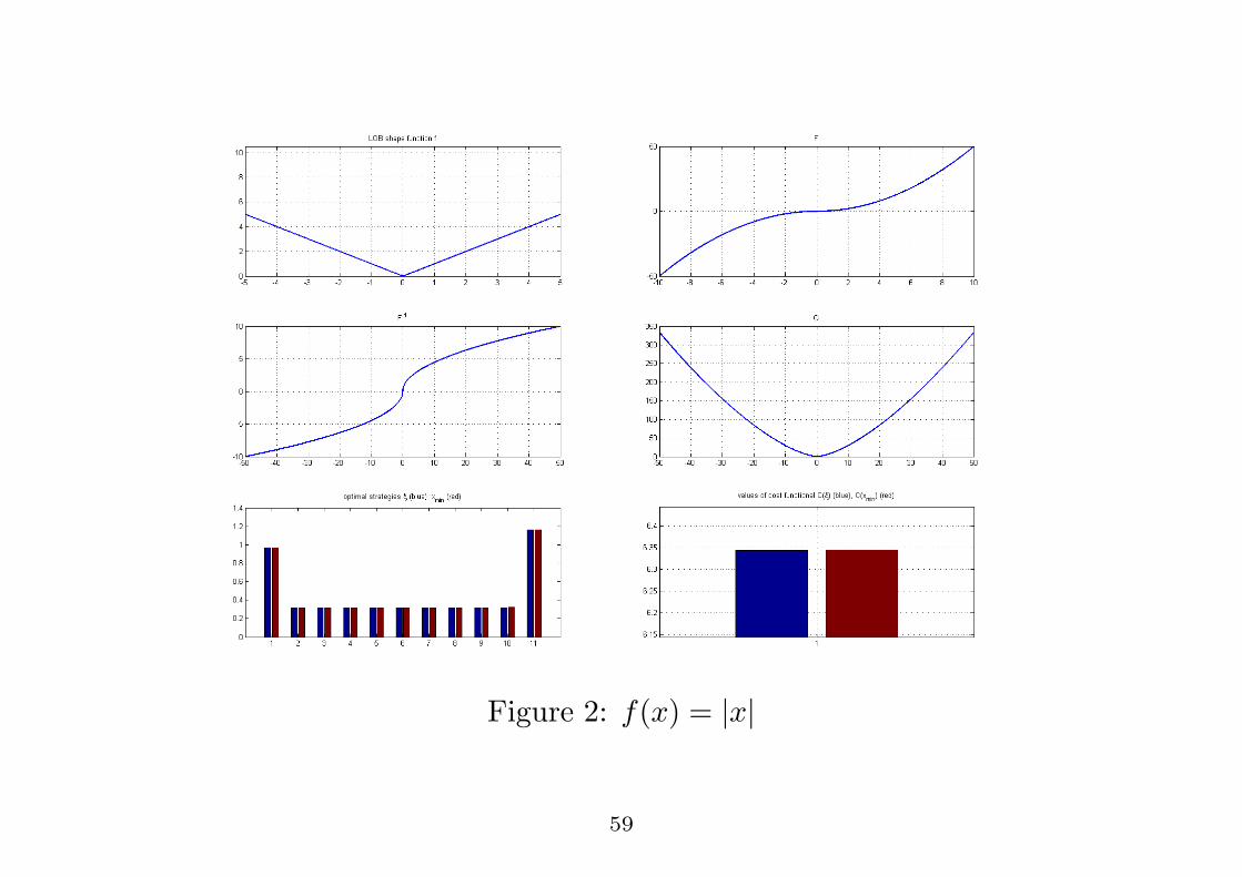
Figure 2: f(x) = |x|
59

Figure 3: f(x) = 18x2
60

Figure 4: f(x) = exp("(|x|" 1)2) + 0.1
61

Figure 5: f(x) = 12 sin(#|x|) + 1
62
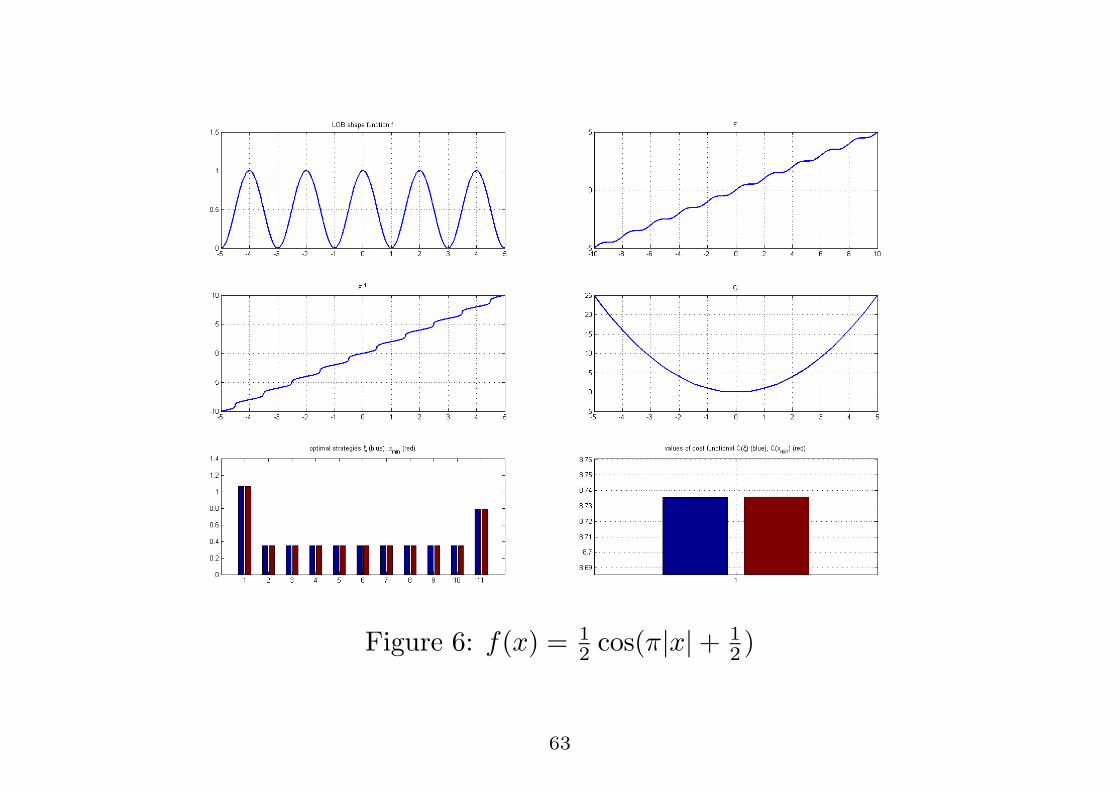
Figure 6: f(x) = 12 cos(#|x| + 1
2 )
63

Figure 7: f random
64

Figure 8: f random
65
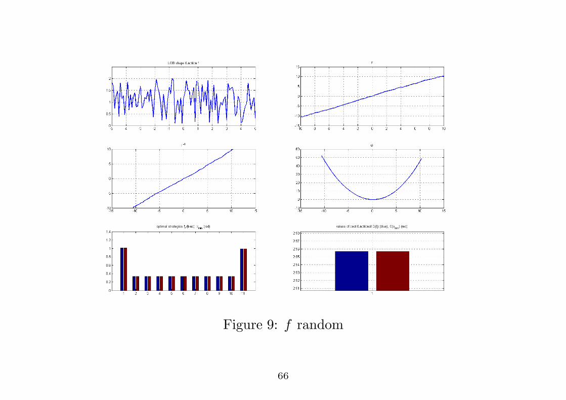
Figure 9: f random
66

Figure 10: f piecewise constant
67
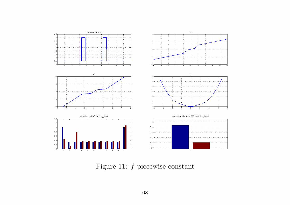
Figure 11: f piecewise constant
68
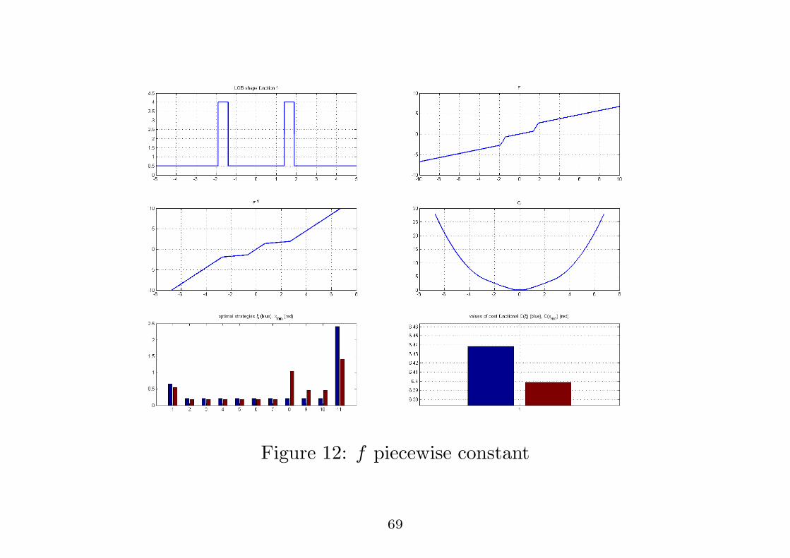
Figure 12: f piecewise constant
69
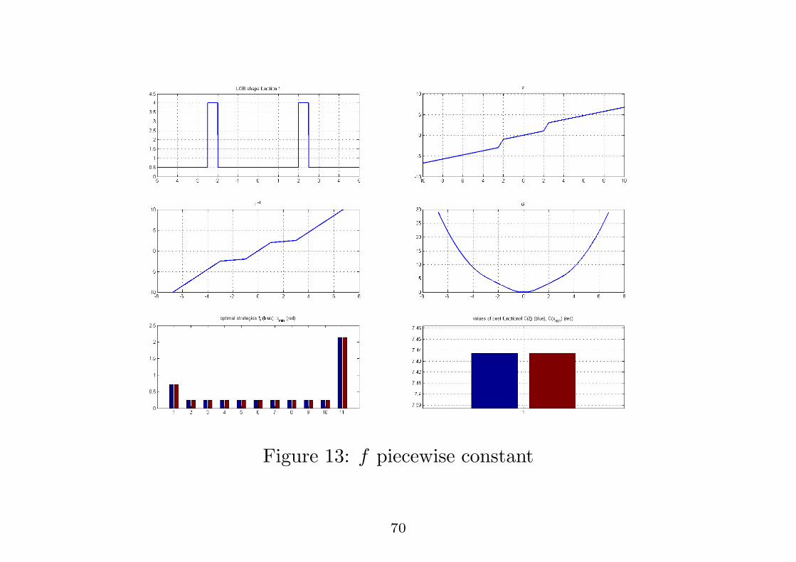
Figure 13: f piecewise constant
70
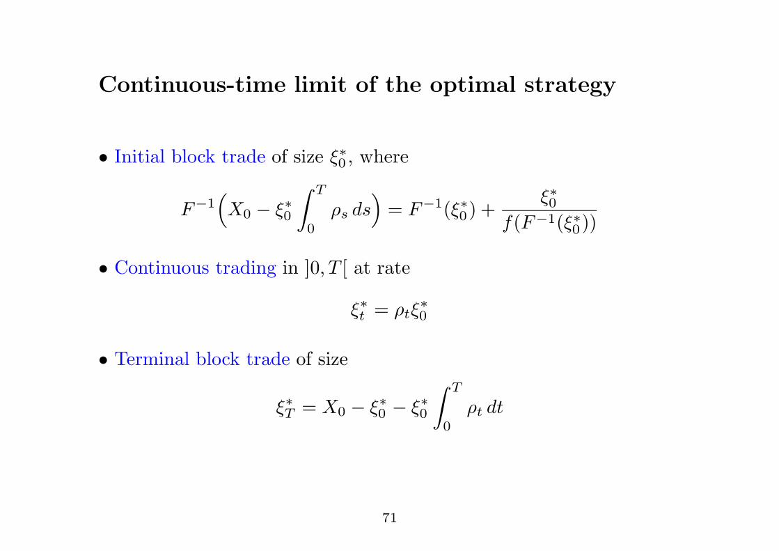
Continuous-time limit of the optimal strategy
• Initial block trade of size !!0 , where
F#1,X0 " !!0
& T
0$s ds
-= F#1(!!0) +
!!0f(F#1(!!0))
• Continuous trading in ]0, T [ at rate
!!t = $t!!0
• Terminal block trade of size
!!T = X0 " !!0 " !!0
& T
0$t dt
71
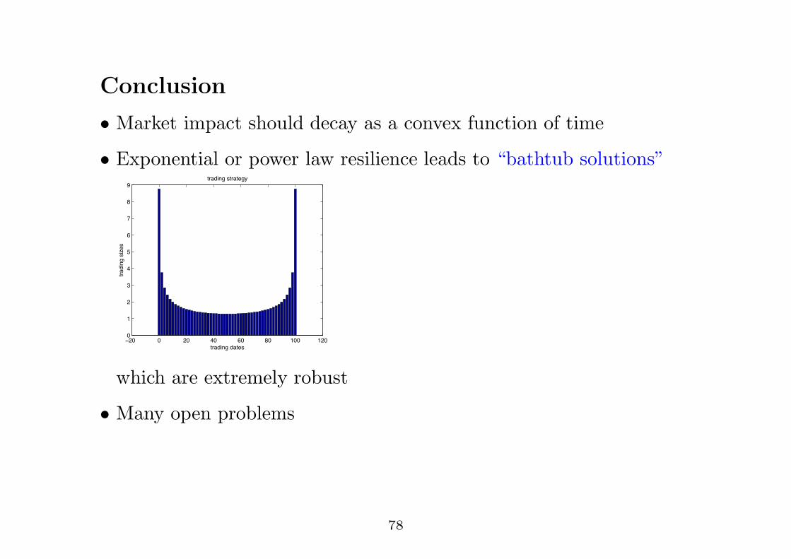
Conclusion
• Market impact should decay as a convex function of time
• Exponential or power law resilience leads to “bathtub solutions”
!!" " !" #" $" %" &"" &!""
&
!
'
#
(
$
)
%
*
+,-./012.-+34
+,-./0124/534
+,-./0124+,-+316
which are extremely robust
• Many open problems
78