ORAL DRUG DELIVERY MOLECULAR DESIGN AND … along with a computer aided technique to generate molecular structures of polymers ... 4.4 Computational Techniques in Computer Aided Molecular

ORAL DRUG DELIVERY – MOLECULAR DESIGN AND TRANSPORT

MODELING

Naresh Pavurala

Dissertation submitted to the faculty of the Virginia Polytechnic Institute and State

University in partial fulfillment of the requirements for the degree of

Doctor of Philosophy

In

Chemical Engineering

Luke E. Achenie, Chairman

Richey M. Davis

Eva Marand

Stephen Martin

November 14, 2013

Blacksburg, VA

Keywords:

Oral drug delivery, drug release model, ACAT model, pharmacokinetic model,

simulation, optimization, molecular design, structure-property models, novel

polymers, release kinetics, oral dosage form, tablet design

VIRGINIA POLYTECHNIC INSTITUTE AND STATE UNIVERSITY

ABSTRACT

Pharmacokinetic Modeling of Oral Drug Delivery

by Naresh Pavurala

Chairperson of the Supervisory Committee: Professor Luke Achenie

Department of Chemical Engineering

One of the major challenges faced by the pharmaceutical industry is to accelerate the product

innovation process and reduce the time-to-market for new drug developments. This involves

billions of dollars of investment due to the large amount of experimentation and validation

processes involved. A computational modeling approach, which could explore the design space

rapidly, reduce uncertainty and make better, faster and safer decisions, fits into the overall goal

and complements the product development process. Our research focuses on the early preclinical

stage of the drug development process involving lead selection, optimization and candidate

identification steps. Our work helps in screening the most favorable candidates based on the

biopharmaceutical and pharmacokinetic properties. This helps in precipitating early development

failures in the early drug discovery and candidate selection processes and reduces the rate of late-

stage failures, which is more expensive.

In our research, we successfully integrated two well-known models, namely the drug

release model (dissolution model) with a drug transport model (compartmental absorption and

transit (CAT) model) to predict the release, distribution, absorption and elimination of an oral drug

through the gastrointestinal (GI) tract of the human body. In the CAT model, the GI tract is

envisioned as a series of compartments, where each compartment is assumed to be a continuous

stirred tank reactor (CSTR). We coupled the drug release model in the form of partial differential

equations (PDE’s) with the CAT model in the form of ordinary differential equations (ODE’s).

The developed model can also be used to design the drug tablet for target pharmacokinetic

characteristics. The advantage of the suggested approach is that it includes the mechanism of drug

release and also the properties of the polymer carrier into the model. The model is flexible and can

iii

be adapted based on the requirements of the clients. Through this model, we were also able to

avoid depending on commercially available software which are very expensive.

In the drug discovery and development process, the tablet formulation (oral drug

delivery) is an important step. The tablet consists of active pharmaceutical ingredient (API),

excipients and polymer. A controlled release of drug from this tablet usually involves swelling of

the polymer, forming a gel layer and diffusion of drug through the gel layer into the body. The

polymer is mainly responsible for controlling the release rate (of the drug from the tablet), which

would lead to a desired therapeutic effect on the body.

In our research, we also developed a molecular design strategy for generating molecular

structures of polymer candidates with desired properties. Structure-property relationships and

group contributions are used to estimate the polymer properties based on the polymer molecular

structure, along with a computer aided technique to generate molecular structures of polymers

having desired properties. In greater detail, we utilized group contribution models to estimate

several desired polymer properties such as grass transition temperature (Tg), density (ρ) and

linear expansion coefficient (α). We subsequently solved an optimization model, which

generated molecular structures of polymers with desired property values. Some examples of new

polymer repeat units are 2 2 nCONHCH CH NHCO ,

nCHOH COO . These repeat-units

could potentially lead to novel polymers with interesting characteristics; a polymer chemist could

further investigate these. We recognize the need to develop group contribution models for other

polymer properties such as porosity of the polymer and diffusion coefficients of water and drug

in the polymer, which are not currently available in literature.

The geometric characteristics and the make-up of the drug tablet have a large impact on

the drug release profile in the GI tract. We are exploring the concept of tablet customization,

namely designing the dosage form of the tablet based on a desired release profile. We proposed

tablet configurations which could lead to desired release profiles such as constant or zero-order

release, Gaussian release and pulsatile release. We expect our work to aid in the product

innovation process.

iv

To my Mother and Father:

Shri Venkateshwara Rao Pavurala

Shri Pushpavathi Pavurala

“Knowing is not enough, we must apply

willing is not enough, we must do…”

― Johann Wolfgang von Goethe

v

Acknowledgements

My Ph.D. program experience was the most challenging, yet enjoyable and rewarding,

academic experience of my life, because I like to learn. It was an overwhelming experience as it

opened my world throughout the years. I have met a lot of wonderful people. I have had the

privilege of working with Dr. Luke Achenie, who was instrumental in helping me to complete

my doctoral work. I sincerely thank him for his unending support and invaluable guidance

throughout the period of my PhD.

I take the opportunity to express my deepest sense of gratitude to Dr. Richie Davis, Dr.

Eva Marand and Dr. Stephen Martin for their constructive criticism, endless help, and

guidance during my period of my PhD work.

I am also very thankful to my colleagues, for their suggestions and support during the

course of my PhD. They include Chris Christie, Zhenxing Wang (Jason), Nuttapol

Lerkkasemsan and Syed Mazahir.

I would like to thank Riley Chan for his ability to fix just about anything and Cannaday

Diane, Nora Bentley, Tina Kirk, Tammy Hiner Jo, Leslie Thornton- O’Brien, Shelley

Johnson, Lois Hall, Dawn Maxey, Lisa Smith ,Ennis McCrery, Ruth Athanson, Graduate

School and Cranwell International Center for their assistance with countless matters.

I also thank the following for financial support: National Science Foundation,

Department of Chemical Engineering, Virginia Tech.

My life at Virginia Tech is priceless and I am really fortunate to know wonderful people

here. I would like to thank Sonal Mazumder, who has supported me through thick and thin - she

had been a great friend, philosopher and guide. I would like to thank my committee (2010-2011)

and members of Indian Students Association in Virginia Tech. I have gained immense

experience and learnt various leadership and teamwork qualities while working with them.

Sincerest thanks to my father, Venkateshwara Rao Pavurala, and mother, Pushpavathi

Pavurala, for being such wonderful parents providing constant support and encouragement.

vi

Thanks to my brother, Sahitya Pavurala and my sister, Swathi Pavurala for everything.

Thanks to my friends in India for all their support and love.

Finally, I would like to thank my professors from Indian Institute of Technology (IIT),

Madras in India, who helped me to follow my dream and pursue my doctoral studies at Virginia

Tech.

Naresh Pavurala

Blacksburg, Virginia-USA

November, 2013

vii

Attribution

Professor Luke Achenie is my research advisor and committee chair. He provided guidance,

help, and support throughout the work in this PhD dissertation. Also he significantly contributed

to the written communication of the research.

viii

TABLE OF CONTENTS

Chapter 1: Introduction

1.1 Drug Delivery ..................................................................................................................... 1

1.2 Problem Statement .............................................................................................................. 5

1.3 References ........................................................................................................................... 8

Chapter 2: Modeling of Drug Release from a Polymer Matrix

2.1 Problem Description ......................................................................................................... 10

2.2 Background and Literature ............................................................................................... 11

2.2.1 Diffusion-controlled systems ............................................................................ 12

2.2.2 Matrix systems .................................................................................................. 13

2.2.3 Swelling-controlled release systems ................................................................. 13

2.2.4 Literature on modeling of tablet swelling and dissolution ............................... 15

2.3 Dissolution model ............................................................................................................. 17

2.4 Solution strategy ............................................................................................................... 21

2.5 Results and Discussion ..................................................................................................... 22

2.6 Conclusions ....................................................................................................................... 28

2.7 Nomenclature .................................................................................................................... 30

2.8 References ......................................................................................................................... 31

Chapter 3: An advanced pharmacokinetic model for oral drug delivery



3.2.1 Advanced Compartmental and Transit (ACAT) Model .................................. 38

3.3 Proposed Methodology ..................................................................................................... 40

3.4 Modeling Strategy ............................................................................................................ 40

3.4.1 Modified Pharmacokinetic Model .................................................................... 40

3.5 Case Study ........................................................................................................................ 43

3.6 Sensitivity Analysis .......................................................................................................... 43

3.7 Model Parameter Estimation ............................................................................................ 46


3.9 Scenarios ........................................................................................................................... 52

ix

3.9.1 Average body weight of a patient ( pW ) ........................................................... 52

3.9.2 Fraction of drug in polymer-drug system ( df ) ................................................ 54

3.9.3 Tablet Radius (R) ............................................................................................. 55

3.9.4 Optimization ...................................................................................................... 56

3.10 Conclusions ..................................................................................................................... 57

3.11 Nomenclature .................................................................................................................. 59

3.12 References ....................................................................................................................... 61

3.13 Appendix A ..................................................................................................................... 64

Chapter 4: Designing polymer structures for oral drug delivery – a molecular design

approach



4.2.1 Polymers in Oral Drug Delivery ....................................................................... 69

4.2.2 Synthetic Biodegradable Polymers ................................................................... 70

4.2.3 Natural Biodegradable Polymers ...................................................................... 72

4.3 Polymer Property Prediction ............................................................................................ 73

4.3.1 Molecular Modeling .......................................................................................... 73

4.3.2 Empirical and Semi-Empirical Models ............................................................ 74

4.3.3 Group / Atom / Bond Additivity ....................................................................... 74

4.4 Computational Techniques in Computer Aided Molecular Design ................................ 76

4.5 CAMD Model Development – Polymers as Drug Carriers ............................................ 76

4.5.1 Properties of Polymers as Drug Carriers .......................................................... 77

4.5.2 Problem Formulation ........................................................................................ 78

4.5.3 Mixed Integer Nonlinear Optimization – Outer Approximation Algorithm ... 81


4.6.1 Ranking of Candidate Polymers ....................................................................... 87

4.6.2 Solubility Parameter Analysis .......................................................................... 91

4.7 Sensitivity and Uncertainty Analysis ............................................................................... 93

4.8 Conclusions ....................................................................................................................... 97

4.9 Nomenclature .................................................................................................................. 100

x

4.10 References ..................................................................................................................... 101

4.11 Appendix A ................................................................................................................... 108

Chapter 5: Customization of Oral Drug Dosage Form – Innovation in Tablet Design

5.1 Problem Description ....................................................................................................... 110

5.2 Background and Literature ............................................................................................. 111

5.2.1 Polymer Matrix Tablet .................................................................................... 112

5.3 Proposed Tablet Designs ................................................................................................ 115

5.3.1 Design 1 – Constant Release Profile .............................................................. 115

5.3.2 Design 2 – Gaussian Release Profile .............................................................. 117

5.3.3 Design 3 – Pulsatile Release Profile ............................................................... 118

5.4 Results and Discussion ................................................................................................... 120

5.5 Conclusions ..................................................................................................................... 122

5.6 References ....................................................................................................................... 123

Chapter 6: Research Summary ..................................................................................................... 125

xi

LIST OF FIGURES

Number Page

Chapter 1: Introduction

Figure 1: Schematic of gastrointestinal tract of human body ........................................................ 3

Figure 2: Schematic of the drug discovery and development process ....................................... 4

Figure 3: Proposed modeling strategy ............................................................................................ 5


Figure 1: Schematic of polymer matrix disentanglement level as a function of polymer

concentration in a swelling-controlled release ............................................................................. 14

Figure 2: Schematic of the drug tablet of initial radius R and initial thickness 2L .................. 18

Figure 3: One-dimensional solvent diffusion and polymer dissolution process ..................... 18

Figure 4: Rate of change tablet interface dimensions G and S for dk value of 0.012 mm/min ....... 22




Figure 8: Effect of polymer degradation rate constants ( dk ) on cumulative (%) drug released.

The total amount of drug released for each of the dk values is a constant of 400 mg ............. 25

Figure 9: Effect of polymer degradation rate constants ( dk ) on drug release rate (dM/dt) ............... 26

Figure 10: Effect of polymer degradation rate constant ( dk ) on the tablet dissolution time ... 28


Figure 1: A typical plasma concentration profile and pharmacokinetic characteristics .......... 36

Figure 2: A schematic of the ACAT model human body .......................................................... 39

Figure 3: Schematic of the modeling methodology ..................................................................... 42

Figure 4: Schematic of the developed pharmacokinetic model ................................................... 42

Figure 5: Molecular Structure of Cimetidine ............................................................................... 43

Figure 6: Comparison of NSC values for the parameters: hepatic clearance rate of drug from

the liver ( hCL ), volume of liver ( liverV ), volume of central compartment ( centralV ) and

absorption coefficient of 2nd compartment ( (2)aK ) ..................................................................... 45

xii

Figure 7: Comparison of model and clinical plasma concentration profiles for (a) 7.5%

methacrylate copolymer cimetidine tablet; (b) 15% methacrylate copolymer cimetidine

tablet; (c) 26% methacrylate copolymer cimetidine tablet, with estimated error bars for

clinical plasma profiles. The experimental error bars are estimated from the standard

deviation values provided in the literature ................................................................................. 50

Figure 8: Comparison of model plasma profiles for different values of patient body weight 53

Figure 9: Comparison of model plasma profiles for different values of fraction of drug ( df )54

Figure 10: Comparison of model plasma profiles for different values of tablet radius .............. 55


approach

Figure 1: CAMD approach in product development process ...................................................... 68

Figure 2: Desirability curve using glass transition temperature (gT ) .......................................... 88

Figure 3: Desirability curve using water absorption (W ) ........................................................... 90

Figure 4: Sensitivity analysis of group contribution parameters ................................................. 95

Figure 5: Uncertainty analysis of group contribution parameters ............................................... 96

Chapter 5: Customization of Oral Drug Dosage Form – Innovation in Tablet Design

Figure 1: Interdependence of plasma profile, drug release profile and tablet design ............... 111

Figure 2: Schematic representation of prolonged release (A), floating (B), and pulsatile release

(C), configurations in a multifunctional drug delivery system composed by HPMC matrices

inserted in an impermeable polymer tube .................................................................................. 114

Figure 3: The Dome Matrix individual and assembled release modules .................................. 115

Figure 4: Constant or zero-order release profile ........................................................................ 116

Figure 5: Tablet configuration for constant release profile – lateral view and cross-section ... 116

Figure 6: Gaussian Release Profile ............................................................................................. 117

Figure 7: Tablet configuration for Gaussian release profile – lateral view and cross-section .. 118

Figure 8: Pulsatile Release Profile .............................................................................................. 119

Figure 9: Tablet configuration for pulsatile release profile – lateral view and cross-section ... 119

Figure 10: Simulated constant release profile for design 1. Constant slope indicates a zero-

order release ................................................................................................................................ 120

xiii

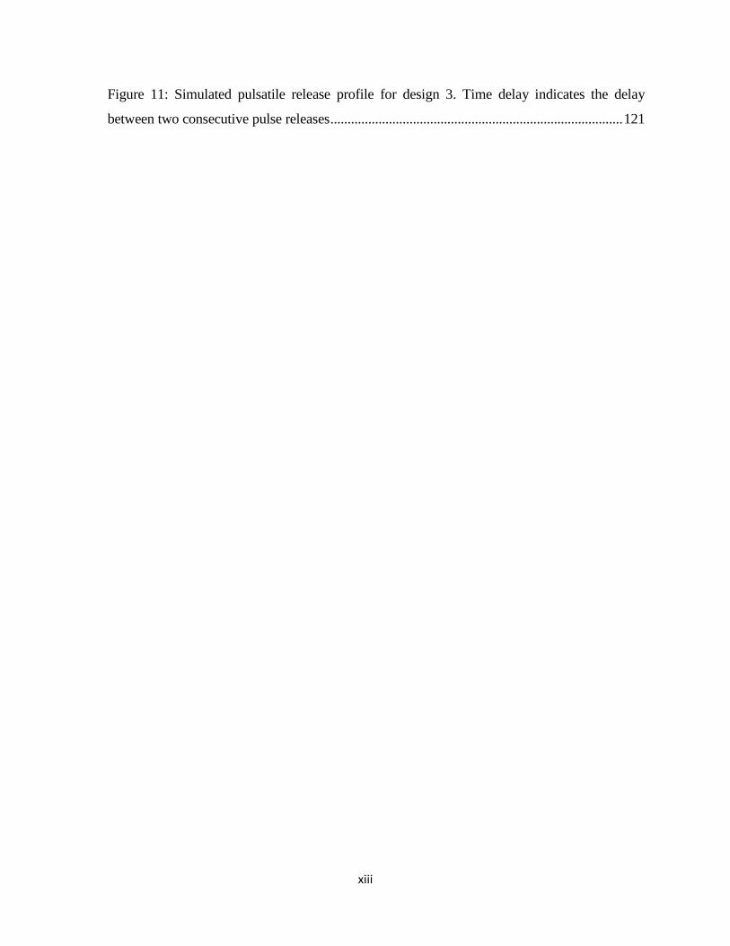
Figure 11: Simulated pulsatile release profile for design 3. Time delay indicates the delay

between two consecutive pulse releases ..................................................................................... 121

xiv

LIST OF TABLES

Number Page


Table 1: Effect of polymer degradation rate on the tablet dissolution time ................................ 27

Table 2: Statistics of the Freundlich curve fitting and parameter values .................................. 27


Table 1: Model Parameters used in the developed pharmacokinetic model............................. 47

Table 2: Compartment parameters used in the modified ACAT model, absorption rate

constants and transit rate constants of each compartment ......................................................... 48

Table 3: Standard deviation and 95% confidence interval values for the estimated parameters 48

Table 4: Comparison of the pharmacokinetic parameters: maxC , maxt , AUC and bioavailability

obtained from both the clinical experiments and the model. Clinical values are expressed as

Value (Standard Deviation) .......................................................................................................... 51

Table A.1: ACAT model compartment parameters for fasted human physiology (Bolger 2009)

....................................................................................................................................................... 66


approach

Table 1: Step by step procedure for formulating a CAMD problem ........................................... 78

Table 2: Basis group set and the respective contributions for different properties ..................... 79

Table 3: CAMD problem formulation ......................................................................................... 83

Table 4: Molecular structures of polymer repeat units and predicted properties ........................ 84

Table 5: Desirability and rank of repeat unit structures using glass transition temperature (gT )

....................................................................................................................................................... 89

Table 6: Desirability and rank of repeat unit structures using water absorption (W ) ................ 90

Table 7: Comparison of solubility parameters of pharmaceutical drugs and generated polymers

....................................................................................................................................................... 92

Table 8: Group contribution parameters and standard deviations for molar glass transition

temperature ................................................................................................................................... 94

Table A1: List of polymers used in drug delivery as carrier materials ..................................... 108

xv

ABBREVIATIONS

CAT Compartmental Absorption and Transit

ACAT Advanced Compartmental Absorption and Transit

AUC Area under the curve

GI Gastrointestinal

ADME Absorption, Distribution, Metabolism and Excretion

NSC Normalized Sensitivity Coefficient

CSTR Continuous Stirred Tank Reactor

PFR Plug Flow Reactor

CAMD Computer Aided Molecular Design

MD Molecular Dynamics

MILP Mixed Integer Linear Programming

MINLP Mixed Integer Nonlinear Programming

API Active Pharmaceutical Ingredient

HPMC Hydroxy Propyl Methyl Cellulose

1

CHAPTER 1

Introduction

1.1 Drug Delivery

Drug delivery can be described as application of chemical and biological principles to control the

in vivo temporal and spatial location of drug molecules for clinical benefit. When a drug is

administered, only a small fraction of the dose actually reaches the relevant receptors or sites of

action, and most of the dose is wasted either by being taken up into the wrong tissue, removed

from right tissue too quickly, or destroyed en route before arrival. The research in drug delivery

is to tackle these issues in order to maximize drug activity and minimize side effects.

Till recently, injections (i.e. intravenous, intramuscular or subcutaneous route) remain the

most common means for administering protein and peptide drugs like insulin. Patient compliance

with drug administration regimens by any of these parenteral routes is generally poor and

severely restricts the therapeutic value of the drug, particularly for disease such as diabetes

(Soltero 2005). Among the alternate routes that have been tried with varying degrees of success

are the oral, buccal (Sayani and Chien 1996), intranasal (Torres-Lugo and Peppas 2000),

pulmonary (O'Hagan DT 1990), transdermal (Banga and Chien 1993), ocular (Lee and

Yalkowsky 1999) and rectal (Pezzuto et al. 1993). Among these, oral route remains the most

convenient way of delivering drugs. Oral administration presents a series of attractive advantages

towards other drug delivery. These advantages are particularly relevant for the treatment of

pediatric patients and include the avoidance of pain and discomfort associated with injections

and the elimination of possible infections caused by inappropriate use or reuse of needles.

Moreover, oral formulations are less expensive to produce, because they do not need to be

manufactured under sterile conditions (Salama et al. 2006). In addition, a growing body of data

suggests that for certain polypeptides such as insulin; the oral delivery route is more

physiological (Hoffman A 1997). It is estimated that 90% of all medicines are oral formulations

and oral drug delivery systems comprise more than half the drug delivery market. In 2008, the

oral drug delivery market was a USD 35 billion industry and was expected to grow as much as

10% per year until at least 2012 (Gabor et al. 2010). Oral drug products are also profitable for the

2

pharmaceutical industry. However, biopharmaceutical issues such as physicochemical

requirements of the drug and physiological conditions make oral delivery one of the most

challenging routes. With recent developments in manufacturing technology, large quantities of

oral formulations are produced with short production times. By following good manufacturing

practices (GMP regulations), high quality oral delivery products are prepared in a reliable and

reproducible manner.

Dissolution and absorption of drugs from the gastrointestinal (GI) tract is a very complex

process involving multiple steps including drug disintegration and dissolution, degradation,

gastric emptying intestinal transit, intestinal permeation and transport, intestinal and hepatic

metabolism (Yu et al. 1996, Martinez and Rilyn 2002, Huang et al. 2009). It is influenced by

many factors that not only vary among various compounds and formulations but also between

different regions in the GI tract with respect to rate and extent of absorption. Absorption

properties also vary from subject to subject and from time to time. The GI tract offers a large

absorption surface and nearly one third of the blood from cardiac output flows through the

gastrointestinal organs making it a very good site for drug absorption (Gabor et al. 2010). Most

of the tablet formulations include a drug enclosed inside a swellable polymer. The delivery of

drugs, peptides or proteins, occurs through a process of continuous swelling of the polymer

carrier that is associated with simultaneous or subsequent dissolution of the polymer carrier. The

drug is usually molecularly dispersed or dissolved in a polymer matrix at low or high

concentrations. As water penetrates the polymer, swelling occurs and the drug is released to the

external environment (Narasimhan and Peppas 1997).

3

Figure 1: Schematic of gastrointestinal tract of human body (cinncinnati 2006)

Designing and formulating a protein and peptide drug for delivery though GI tract

requires a multitude of strategies. The dosage form must initially stabilize the drug making it

easy to take orally (Sayani and Chien 1996). It must then protect the drug from the extreme

acidity and action of pepsin in the stomach. In the intestine, the drug should be protected from

the surplus amount of enzymes that are present in the intestinal lumen. In addition, the

formulation must facilitate both aqueous solubility at near-neutral pH and lipid layer penetration

in order for the protein to cross the intestinal membrane and then basal membrane for entry into

the bloodstream (Fig. 1). A primary objective of oral delivery systems is to protect protein and

peptide drugs from acid and luminal proteases in the GIT. To overcome these barriers, several

formulation strategies are being investigated. Some of them include enteric-coated dry

emulsions, microspheres, and nanoparticles for oral delivery of peptides and proteins.

4

The drug discovery and development process involves several stages to bring a new drug

(new chemical entity (NCE)) from laboratory to market. These include, target/disease

identification, hit identification/discovery, hit optimization, lead selection and further

optimization, candidate identification and clinical trials (Kuhlmann 1997). It involves

identification and screening of tens of thousands of compounds to identify a few candidates (hits)

with desired biological activity. These hits are further filtered based on their efficiency, and then

tested in various pharmacological models. These candidates (leads) are further optimized based

on their biopharmaceutical properties and filtered down to one or two best drug-like candidates

for further development (Han and Wang 2005). Clinical trials are done on these drug like

candidates of which only one compound makes to the market. Fig. 2 shows a schematic

description of the drug discovery and development process along with a rough estimate of the

number of candidates after each step.

Figure 2: Schematic of the drug discovery and development process (Han and Wang 2005)

The entire drug discovery and development process costs around a billion dollars to bring

a single new drug from laboratory to m/rket. This involves a lot of candidate failures to the early

and late stages in the process. It was estimated that 39% of the failure was due to poor

pharmacokinetic properties in humans; 29% was due lack of clinical efficiency; 21% was due to

toxicity and adverse effects and 6% due to commercial limitations (Han and Wang 2005). The

preclinical stage research includes about tens of million dollars of the total cost, whereas the

clinical trials cost hundreds of millions of dollars. Therefore, a significant improvement in the

Compound Library

(100,000 compounds)

In vitro activity

Hits

(100 compounds)

Efficacy and developability

Leads

(10 compounds)

Candidate selection

Drug candidates

(1-2 compounds)

IND, clinial trial and NDA

Marketed medicine

5

efficiency of the preclinical stage process will reduce potential failures in the later stages of the

process and also save millions of dollars.

1.2 Problem Statement

In this dissertation we are trying to address the issue of reducing the number of experimental

trials, time and effort needed for drug design and development. This work will help aid in the

preclinical stage of the drug discovery and development process and help in reducing potential

failures in the later stages. To address the stated issue we proceed as follows. We propose to

accomplish a two way modeling approach i.e., given a drug tablet with initial dosage, the model

can predict the pharmacokinetic behavior of the drug inside the body and its plasma

concentration profile. Inversely, given the pharmacokinetic characteristics; the model can

evaluate the design parameters and dosage of the drug tablet (Fig. 3).

Figure 3: Proposed modeling strategy

We have defined the following aims to accomplish this task:

Aim 1

Develop a drug release model to predict the release of drug from an oral dosage form (drug

enclosed in a polymer matrix) into the gastrointestinal (GI) tract of the human body

6

Aim 2

Develop a modeling platform to predict the plasma concentration profile and pharmacokinetic

characteristics of an oral drug, given a drug release profile

Aim 3

Develop a modeling strategy to design the drug tablet using structure-property models and

molecular design for a desired drug release profile

Aim 4

Design different dosage forms of the tablet to obtain specific desired drug release profiles –

Tablet customization

In this thesis, the four specific aims are described in greater detail in chapters 2, 3, 4 and

5 respectively.

In chapter 2, we discuss a drug release model which predicts the release of drug from an

oral drug tablet (drug enclosed in a polymer matrix) when it is taken into the gastrointestinal (GI)

tract (Aim 1). This chapter discusses the various factors that influence the drug release and the

effect of polymer matrix on the drug release. This work is expected to be very useful in the tablet

design process.

After successfully developing a working drug release model, we develop a

pharmacokinetic model which predicts the behavior of the drug as it passes through the GI tract

in chapter 3 (Aim 2). The pharmacokinetic model is a combination of the drug release model

developed in chapter 2 with a drug transport model. The developed model will be able to predict

the plasma concentration profile and other pharmacokinetic characteristics such as peak plasma

concentration, area under the curve and bioavailability. The plasma concentration profile

represents the obtained therapeutic effect in the patient. This work is expected to be very useful

in the drug discovery and development process.

Through Aim 1 and Aim 2, we were able to accomplish the forward problem as discussed

in Fig. 3. Given a drug tablet, through the drug release model and the pharmacokinetic model

developed in chapters 1 and 2, we will be able to predict the personal pharmacokinetic

7

characteristics of a patient. In the subsequent chapters, we tried to accomplish the reverse

problem, i.e., developing the tablet formulation, given the personal pharmacokinetic

characteristics.

In Chapter 4, we proposed a computer aided molecular design (CAMD) strategy which

could aid in the drug tablet formulations. In this work, we specifically worked on the polymer

component in the drug tablet. The polymer inside the tablet is majorly responsible for controlling

the release rate of the drug from the tablet, hence controlling the drug release profile. A desired

drug release profile is inspired by a desired plasma concentration profile. Through this approach,

we were able to generate molecular structures of polymers which could be used as potential

carrier materials for oral drugs. This work is expected to aid in the product development process.

In chapter 4, we discussed the concept of tablet customization, i.e., designing the dosage

form of the drug tablet according to a desired drug release profile. In this work, we proposed

tablet configurations which could lead to a desired release profiles such a constant release

profile, a Gaussian release profile and a pulsatile release profile. The tablet design greatly

influences the release characteristics. Tablet configurations could be customized based on the

requirement of the patient, his physiological and genetic makeup, and the desired therapeutic

effect. This work will greatly improve the patient compliance, reduce side effects, reduce dosage

frequency and improve the overall efficiency of the drug tablet. This work is a significant

forward step towards the development of personalized medicine.

8

1.3 References

Banga, A. K. and Y. W. Chien (1993). "Hydrogel-Based lontotherapeutic Delivery Devices for

Transdermal Delivery of Peptide/Protein Drugs." Pharmaceutical Research 10(5): 697-702.

cinncinnati, G. c. o. g. (2006). "Your digestive system and how it works ", from

http://ssl.gcis.net/giconsults/gi-tract.htm.

Gabor, F., C. Fillafer, L. Neutsch, G. Ratzinger and M. Wirth (2010). Improving Oral Delivery

Drug Delivery. M. Schäfer-Korting, Springer Berlin Heidelberg. 197: 345-398.

Han, C. and B. Wang (2005). Factors That Impact the Developability of Drug Candidates: An

Overview. Drug Delivery, John Wiley & Sons, Inc.: 1-14.

Hoffman A, Z. E. (1997). "Pharmacokinetic considerations of new insulin formulations and

routes of administration." Clin Pharmacokinet. 33(4): 285-301.

Huang, W., S. Lee and L. Yu (2009). "Mechanistic Approaches to Predicting Oral Drug

Absorption." The AAPS Journal 11(2): 217-224.

Kuhlmann, J. (1997). "Drug research: from the idea to the product." Int J Clin Pharmacol Ther

35(12): 541-552.

Lee, Y.-C. and S. H. Yalkowsky (1999). "Effect of formulation on the systemic absorption of

insulin from enhancer-free ocular devices." International Journal of Pharmaceutics 185(2): 199-

204.

Martinez, M. a. and Rilyn (2002). "A Mechanistic Approach to Understanding the Factors

Affecting Drug Absorption: A Review of Fundamentals." Journal of clinical pharmacology

42(6): 620-643.

Narasimhan, B. and N. A. Peppas (1997). "Molecular analysis of drug delivery systems

controlled by dissolution of the polymer carrier." Journal of Pharmaceutical Sciences 86(3): 297-

304.

9

O'Hagan DT, I. L. (1990). "Absorption of peptides and proteins from the respiratory tract and the

potential for development of locally administered vaccine." Crit Rev Ther Drug Carrier Syst.

7(1): 35-97.

Pezzuto, J. M., M. E. Johnson and H. Manasse Jr (1993). Biotechnology and pharmacy,

Chapman & Hall.

Salama, N. N., N. D. Eddington and A. Fasano (2006). "Tight junction modulation and its

relationship to drug delivery." Advanced Drug Delivery Reviews 58(1): 15-28.

Sayani, A. P. and Y. W. Chien (1996). "Systemic Delivery of Peptides and Proteins Across

Absorptive Mucosae." Critical Reviews in Therapeutic Drug Carrier Systems 13(1&2): 85-184.

Soltero, R. (2005). Oral Protein and Peptide Drug Delivery. Drug Delivery, John Wiley & Sons,

Inc.: 189-200.

Torres-Lugo, M. and N. A. Peppas (2000). "Transmucosal delivery systems for calcitonin: a

review." Biomaterials 21(12): 1191-1196.

Yu, L. X., E. Lipka, J. R. Crison and G. L. Amidon (1996). "Transport approaches to the

biopharmaceutical design of oral drug delivery systems: prediction of intestinal absorption."

Advanced Drug Delivery Reviews 19(3): 359-376.

10

CHAPTER 2

Modeling of Drug Release from a Polymer Matrix System

Abstract

A drug release model is proposed to predict the behavior of an oral drug tablet when it is taken

through the gastrointestinal (GI) tract. The model predicts the rate of change of tablet dimensions.

The effect of polymer degradation rate on the tablet dissolution time and drug release kinetics was

analyzed. The total tablet dissolution time decreased with increase in the polymer degradation rate

constant ( dk ). A power law model was fit to describe the relationship between tablet dissolution

time and dk . The model predicted initial burst release of the drug followed by a constant release.

The time of burst release and the amount of drug undergoing burst release decreased with increase

in dk value.

Keywords: drug release model, drug diffusion, polymer matrix swelling, polymer dissolution,

release kinetics

2.1 Problem Description

In this chapter, we propose a model to predict the release behavior of an oral drug from the solid

drug tablet inside the GI tract of the human body. The model should be able to predict the amount

of drug released into various regions of the GI tract. The model will provide insights on the various

mass transport and chemical processes involved in drug delivery, as well as the effect of tablet

design, geometry and drug loading on the release mechanism involved. The release behavior of a

drug determines the pharmacokinetic behavior of the drug in the plasma. The proposed model will

be a prelude to the development of the pharmacokinetic model discussed in chapter 3.

To address the problem as stated above, we employ a mechanistic modeling approach to

construct the model. Mechanistic modeling takes into account the physical mechanisms that

influence the process to develop the model. Therefore, it helps in better understanding of the

processes which are difficult to explain experimentally. In this work, we developed a drug release

11

model based on the dissolution model proposed by Narasimhan and Peppas (Narasimhan and

Peppas 1997, Brazel and Peppas 2000, Narasimhan 2001).

2.2 Background and Literature

There has been a significant change in the performance of drug delivery systems in the last 100

years. The delivery systems have evolved from simple pills to sustained/ controlled release and

sophisticated programmable delivery systems (Grassi and Grassi 2005). Uncontrolled and

immediate drug release kinetics is the characteristic of traditional delivery systems. This mainly

led to abrupt increase in drug concentration on body tissues crossing the toxic threshold and then

falling off below the minimum effective therapeutic level. The development of controlled drug

delivery systems has greatly helped in solving this issue, and in maintaining the drug concentration

in the blood and other tissues at a desired level for a longer time. In a controlled drug release

system, a burst of drug is initially released to rapidly obtain the drug effective therapeutic

concentration and then follows a controlled release behavior to maintain the drug concentration at

the desired level. The development of controlled release systems has greatly improved patient

compliance and drug effectiveness. They helped in reducing the dosage administration frequency

and prevent side effects. Thus the design and development of controlled release systems has

become a key issue in modern day research. Many engineers and pharmacists have come together

to design and develop effective delivery systems. The use of mathematical modeling in this process

is a very useful approach. It helps in predicting the drug release kinetics from a controlled release

system and helps in further improving the design and development process.

The most common strategy to obtain a controlled drug release is by embedding a drug in a

polymer matrix. The polymer used for this purpose can be a hydrophobic or a hydrophilic matrix

depending on the nature of the drug. Some of the hydrophobic polymers include wax,

polyethylene, polypropylene and ethylcellulose. Some of the hydrophilic polymers are

hydroxypropylcellulose, hydroxypropylmethylcellulose, methylcellulose, sodium

carboxymehylcellulose, alginates and scleroglucan (Finch 1995).

The drug release mechanism from a polymer matrix can be categorized based on three

different processes, which are:

1) Drug diffusion from a non-biodegradable polymer (diffusion-controlled system)

12

2) Drug diffusion from a swellable polymer (swelling-controlled system)

3) Drug release due to polymer degradation and erosion (erosion-controlled system)

All the above-mentioned processes have a diffusion component. For a non-biodegradable

polymer matrix, drug release is due to the concentration gradient caused by diffusion or polymer

swelling. For a biodegradable polymer matrix, release is either controlled by polymer chain

disentanglement which leads to matrix erosion or by diffusion when the erosion process is slow

(Leong and Langer 1988, Fu and Kao 2010). There are several mathematical models proposed for

drug release from tablets of different geometries as discussed above (Cabrera and Grau 2007,

Siepmann and Siepmann 2008).

2.2.1 Diffusion-controlled systems

Diffusion-controlled systems are generally modeled using Fick’s law of diffusion with appropriate

boundary conditions. For example, the diffusion from a spherical micro particle is given by Eq. 1.

2

2

1(1)

C CDr

t r r r

where, the diffusion is assumed to be in the radial direction, D and C are the diffusion coefficient

and the concentration of the drug in the polymer matrix. The boundary conditions are based on the

mass transfer processes at the surface and the bulk surrounding the micro particle.

A reservoir system is a very good example of a diffusion-controlled system. In that system,

the assumption is that the drug is confined in a spherical shell of inner radius (Ri) and outer radius

(Ro) and the diffusion of drug takes place through the shell thickness of (Ro – Ri). The Fick’s law

defined in Eq. 1 is solved, with boundary conditions defined as in Eq. 2,

0

i r

o

r R C C

r R C

(2)

where, the concentration of drug at the inner radius (Ri) is kept at a constant reservoir drug

concentration (Cr) and the concentration at the outer radius (Ro) is assumed to be zero, since the

surrounding bulk volume is large and there is no other mass transfer limitation (Arifin et al. 2006).

13

2.2.2 Matrix systems

In a typical matrix system, the drug is uniformly distributed within a non-biodegradable polymer

matrix. The mechanism of drug release from a matrix system is dependent on the initial drug

loading of the tablet and the solubility of drug in the polymer matrix. When the initial drug loading

is lower than the drug solubility, the drug is assumed to be uniformly distributed in the polymer

matrix. These kinds of systems are known as dissolved drug systems. In contrast, in a dispersed

drug system the initial drug loading is higher than the drug solubility inside the polymer system.

Here the system is divided into two regions namely, the non-diffusing region, where the

undissolved drug is at the initial drug loading concentration and the diffusion region where the

diffusion of the dissolved drug takes place. The drug diffusion through the diffusion region leads

to shrinking of the non-diffusing region. Thus the boundary between the non-diffusing and the

diffusing region continuously moves making it a moving-boundary problem (Arifin et al. 2006,

Wu and Brazel 2008).

2.2.3 Swelling-controlled release systems

Swelling-controlled systems generally consist of a uniformly distributed drug within a

biodegradable, swellable polymer. These swellable polymers are hydrophilic in nature so that

when in contact with water, the latter is absorbed into the polymer, thereby swelling the polymer

matrix. The swelling helps in loosening the polymer entanglement leading to disentanglement of

the polymer. The polymer matrix swelling leads to the formation of a rubbery region, where there

is better drug mobility due to lower polymer concentration. This helps in enhancing the release

characteristics of the drug which is not only dependent on the diffusion rate of the drug but also

on the polymer disentanglement and dissolution processes. A schematic showing the effect of

polymer concentration on the polymer disentanglement rate is shown in Fig. 1.

14

Figure 1: Schematic of polymer matrix disentanglement level as a function of polymer concentration in a

swelling-controlled release system (redrawn from (Ju et al. 1995))

As the polymer absorbs water, there is a change in concentration of the polymer in the

matrix. The polymer concentration is very high in the dry glassy core. The water diffusion in the

swollen glassy layer creates a more mobile network, but restricted by very strong chain

entanglement. In the gel layer, the concentrations of water and polymer become comparable with

some reduction in the chain entanglement. Ultimately, the diffusion layer becomes very rich in

water concentration, leading to weak chain entanglement and the polymer starts to disentangle and

dissolve at the interface (Arifin et al. 2006).

15

2.2.4 Literature on modeling of tablet swelling and dissolution

The modeling of drug release from polymer matrices can greatly improve the design and

understanding of delivery systems. Availability of a reliable mathematical model could

complement/augment the resource-consuming trial and-error procedures usually followed in the

manufacture of drug delivery systems. Several modeling approaches are presented in the literature;

those that are relevant to this work are described below.

Modeling drug release behavior by swelling and dissolving in polymer matrices described

in the literature considers either polymer slabs or spheres (Mallapragada and Peppas 1997,

Narasimhan and Peppas 1997); very few models consider the cylindrical geometry of tablets

(Siepmann et al. 1999, Siepmann et al. 1999, Siepmann et al. 2000, Siepmann and Peppas 2000,

Siepmann et al. 2002). Tablet models tend to employ simplified one-dimensional transport

assumptions (Ju et al. 1995, Kiil and Dam-Johansen 2003).

The model by Borquist et al. (Borgquist et al. 2006) considered drug release from a

swelling and dissolving cylindrical polymeric tablet and can predict drug release from

formulations containing soluble as well as poorly soluble drugs. The mass transfer rate includes

the contributions from diffusion as well as swelling (diffusion induced convection). The

transformation from solid to gel phase is assumed to be limited by the rate of penetrant transport

into the solid phase, corresponding to a critical penetrant concentration. At the gel–solvent

interface, it is assumed that equilibrium exists between the hydrodynamic forces and polymer

entanglement. This implies that the surface polymer concentration reaches a constant value after

the initial phase, and that this equilibrium exists for the rest of the dissolution process. Hence, the

initial polymer dissolution rate is zero, until the entanglement strength has been reduced by the

increased penetrant concentration. The model was used to study the influence of the drug diffusion

coefficient, the drug solubility and the initial drug loading on the drug release profile. The model

presented in this paper can simulate the drug and polymer release from swelling and dissolving

polymer tablet. The model was verified against drug release and polymer dissolution data for the

slightly soluble drug Methyl Paraben and the soluble drug Saligenin, showing good agreements in

both cases. The drug diffusion coefficient was fitted to data, and the values obtained were

considered to be accurate, thus confirming the reliability of the model.

16

The immersion of pure Hydroxypropylmethylcellulose (HPMC) tablets in water and their

water uptake, swelling and the erosion during immersion were investigated in drug-free and drug-

loaded systems (Chirico et al. 2007). A novel approach by image analysis to measure polymer and

water masses during hydration was described. It was found that that the model consisting in the

transient mass balance, accounting for water diffusion, diffusivity change due to hydration,

swelling and erosion, was able to reproduce experimental data.

In Kill et al. (Kiil and Dam-Johansen 2003), a detailed mathematical model capable of

estimating radial front movements, transient drug fluxes, and cumulative fractional drug release

behaviors from a high-viscosity HPMC matrix was presented. Simulations produced with the

model were compared to the measurements reported by Bettini et al. (Bettini et al. 1994, Bettini et

al. 2001) and Colombo et al. (Colombo et al. 1999). However the model could not describe the

continued swelling of the matrix, subsequent to the disappearance of the swelling front. Models of

drug release from hydrogel based matrices of HPMC were presented by Lamberti et al. (Lamberti

et al. 2011).

The effect of polymer relaxation constant on water uptake and drug release was shown in

a mathematical model for the simulation of water uptake by and drug release from homogeneous

poly-(vinyl alcohol) hydrogel (Wu and Brazel 2008). Another work showed that swelling of the

hydrogel carrier begins from the edge to the center. At the beginning the drug release is by

anomalous transport followed by Fickian diffusion when the swelling of the hydrogel approaches

to a new equilibrium state (Zhang and Jia 2012).

A mathematical model was developed to describe the transport phenomena of a water-

soluble small molecular drug (caffeine) from highly swellable and dissoluble polyethylene oxide

(PEO) cylindrical tablets (Wu et al. 2005).The work considered several important aspects in drug

release kinetics such as swelling of the hydrophilic matrix and water penetration, three-

dimensional and concentration-dependent diffusion of drug and water, and polymer dissolution.

In vitro study of swelling, dissolution behavior of PEOs with different molecular weights and drug

release were carried out. When compared with experimental results, this theoretical model agreed

with the water uptake, dimensional change and polymer dissolution profiles very well for pure

PEO tablets with two different molecular weights. Drug release profiles using this model were

predicted with a very good agreement with experimental data at different initial loadings. The

17

overall drug release process was highly dependent on the matrix swelling, drug and water

diffusion, polymer dissolution and initial dimensions of the tablets. When their influences on drug

release kinetics from PEO with two different molecular weights were investigated, it was found

that swelling was the dominant factor in drug release kinetics for higher molecular weight of PEO

(Mw=8×106) while both swelling and dissolution were important to caffeine release for lower

molecular weight PEO (Mw=4×106). It was found that when initial drug loading increases,

polymer dissolution became more and more important in the release process. Besides swelling and

dissolution properties of polymer, the ratio of surface area to volume and the aspect ratio of initial

tablets were found to be influential in the overall release profile.

A novel method was developed by Kimber et. al. (Kimber et al. 2012) to simulate polymer

swelling and dissolution by combining a discrete element method (DEM) with inter-particle mass

transfer. The method was applied to simulate the behavior of cylindrical tablets. The model

considered the effects of several parameters such as the concentration-dependent diffusion

constant of water in polymer, dissolution rate constant of polymer and the disentanglement

threshold of polymer on the tablet behavior. A new drug component was included in the DEM

method and the effects of drug distribution, maximum swelling ratio of polymer and drug-polymer

diffusivity on the tablet behavior were studied (Kimber et al. 2013). The model was able to

explicitly define the drug distribution in the tablet. The model showed that for a homogeneously

dispersed drug, the release was slow over time, but for a heterogeneous distribution, there was an

initial burst release followed by a slower release.

2.3 Dissolution Model

The Dissolution Model (Narasimhan and Peppas 1997, Brazel and Peppas 2000, Narasimhan

2001) explains the release of a water soluble, crystalline drug enclosed within a swellable,

hydrophilic glassy polymer, placed in contact with water or a biological fluid. It is a moving

boundary problem formulated using a system of partial differential equations (PDE’s) and ordinary

differential equations (ODE’s) which describe the (i) diffusion of water into the system; (ii)

diffusion of drug out of the system; (iii) polymer chain disentanglement through the boundary

layer and (iv) the left and right moving boundaries. All the diffusion processes take place along

the tablet thickness indicated by X (Fig. 2) making it a 1-D problem in space.

18

Figure 2: Schematic of the drug tablet of initial radius R and initial thickness 2L

Figure 3: One-dimensional solvent diffusion and polymer dissolution process (Narasimhan and Peppas

1997)

In this model, when water comes in contact with the glassy polymer of initial thickness 2L

(Fig. 3a), the polymer starts to swell and two distinct fronts are formed: the swelling interface at

position G , and the polymer-water interface at position S (Fig. 3b). Initially, the front G moves

inwards since the drug starts diffusing out of the gel layer and the front S moves outwards due to

polymer swelling. When the concentration of water inside the polymer gel layer exceeds a critical

value, *

1v , polymer disentanglement begins and S starts to diminish. Hence, during the latter stage

of the dissolution process, both G and S move towards the center of the tablet (Fig. 3c). The

process continues, till the glassy core disappears and only the front S exists, which continues to

diminish till the entire polymer is dissolved (Fig. 3d). A detailed description of the various

equations used in the modeling of the dissolution model is given below.

Water transport into the polymer matrix is expressed using Fick’s law as:

1 11 (3)

v vD G x S

t x x

19

where, is the volume fraction of water in the swollen polymer, is the diffusion coefficient of

water in polymer and x is dimension along the tablet thickness. Eq. 3 is valid in the slab region

between G and S (see Fig. 3b and Fig. 3c). The diffusion of drug out of the polymer is given by:

(4)d dd

v vD G x S

t x x

Here, is the volume fraction of drug in the swollen polymer and is the drug diffusion

coefficient in the polymer. Eq. 3 and 4 describe the overall swelling/dissolution/release process

and are solved with the following initial conditions

1 0( ,0) 0 ( ,0) (5)d dv x v x v

The first boundary condition for Eq. 3 and 4 is at the glass-rubbery interface G , given by:

* *

1 1( , ) ( , ) (6)d dv G t v v G t v

The critical volume fractions of water and drug at the interface, G , are and , respectively.

Here and are functions of the thermodynamic conditions of glassy-rubbery transition, given

by:

* * *

1 21 (7)dv v v

* 22

2 1

1

(8)( )1 1 1

( / )

g

f d

vT T

*

2 1

1

(9)( )1 1 1

( / )

dd

g

f d

vT T

where, Tg is the glass transition temperature, T is the experimental temperature, f is the linear

expansion coefficient of the polymer, is the expansion coefficient contribution of water to

1v 1D

dv dD

*

1v *

dv

*

1v *

dv

20

polymer, 1 is the water density, 2 is the polymer density and d is the drug density. The second

boundary condition for Eq. 3 and 4 is at the rubbery-solvent interface, S , given by:

1 1, ,( , ) ( , ) (10)eq d d eqv S t v v S t v

where and are the equilibrium volume fractions of water and drug, estimated using the

Flory-Rehner equation (Paul J. Flory 1943).

A mass balance at the interface G gives the moving boundary condition at the glassy-

rubbery interface:

11 1( , )

( , ) ( , )

( ) (11)dd dG t

G t G t

vvdGv v D D

dt x x

The initial condition for Eq. 11 is given by, (0)G L , where L is the initial half thickness of the

tablet. The values of 1v and dv at interface G are given by Eq. 6. A mass balance at the interface

S gives the moving boundary condition at the water-rubbery interface:

1 21 1 1( , )

( , ) ( , )( , )

( ) (12)dd d d pS t

S t S tS t

vv vdSv v D v D v D

dt x x x

The initial condition for Eq. 12 is given by, (0)S L . The values of 1v and dv at interface S are

given by Eq. 10.

As the polymer chains disentangle, they move out of the gel layer through a diffusion

boundary layer (semi-dilute regime) of thickness b . The polymer chain transport through this

boundary layer is given by:

2 2 (13)dp b

vv v dSD S x S

t x x dt x

The initial and boundary conditions to Eq. 13 are given by:

1,eqv ,d eqv

21

2

2

2

( , )

2

( , )

2 2,( , )

( ,0) 0 (14)

( , ) 0 (15)

0 0 (16)

(17)

(18)

b

p rept

S t

p d rept c

S t

eq cS t

v x

v S t

vD t t

x

vD k t t t

x

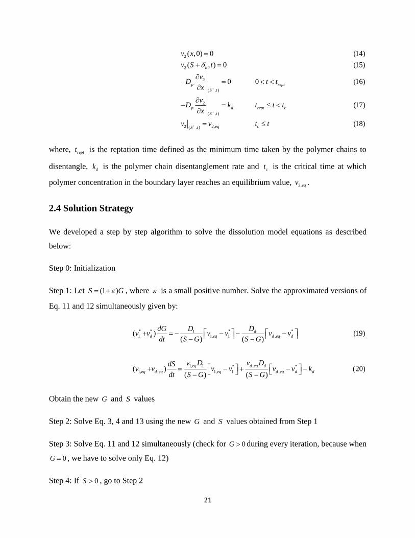
v v t t

where, reptt is the reptation time defined as the minimum time taken by the polymer chains to

disentangle, dk is the polymer chain disentanglement rate and ct is the critical time at which

polymer concentration in the boundary layer reaches an equilibrium value, 2,eqv .

2.4 Solution Strategy

We developed a step by step algorithm to solve the dissolution model equations as described

below:

Step 0: Initialization

Step 1: Let (1 )S G , where is a small positive number. Solve the approximated versions of

Eq. 11 and 12 simultaneously given by:

* * * *11 1, 1 ,( ) (19)

( ) ( )

dd eq d eq d

DDdGv v v v v v

dt S G S G

1, 1 ,* *

1, , 1, 1 ,( ) (20)( ) ( )

eq d eq d

eq d eq eq d eq d d

v D v DdSv v v v v v k

dt S G S G

Obtain the new G and S values

Step 2: Solve Eq. 3, 4 and 13 using the new G and S values obtained from Step 1

Step 3: Solve Eq. 11 and 12 simultaneously (check for 0G during every iteration, because when

0G , we have to solve only Eq. 12)

Step 4: If 0S , go to Step 2

22

2.5 Results and discussions

We successfully solved the dissolution model using the modified strategy. The solution is divided

into two parts. The first part of the solution includes solving for both G and S until the value of

G (thickness of the solid drug tablet) becomes zero. The second part involves solving only for S

(thickness of the swollen polymer) after G is zero. Here the contribution of water diffusion to the

swelling of the polymer is negligible, only including the drug diffusion and the polymer

disentanglement terms resulting in diminishing of S .

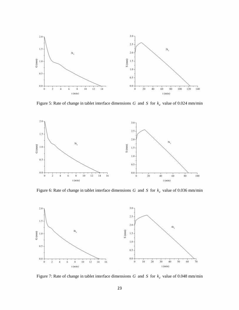
We first studied the effect of polymer disentanglement rate constant ( dk ) on the rate at

which the tablet dimensions G and S vary inside the body. The value of dk has been varied by

different factors and plotted curves showing the rate of change of G and S with time. Fig. 4, 5, 6

and 7 show the rate of change of G and S with increasing dk values of 0.012, 0.024, 0.036 and

0.048 mm/min, respectively.

Figure 4: Rate of change in tablet interface dimensions G and S for dk value of 0.012 mm/min

23




24

Here G is a measure of the solid tablet thickness and S is a measure of the total tablet

thickness along with the swollen polymer. An expected trend is observed both in the case of G

and S as discussed in section 2.3. The solid tablet thickness ( G ) decreases with time as the tablet

traverses through the GI tract and comes into contact with the bodily fluid. This is due to the

continuous diffusion of drug out of the solid tablet and the conversion of solid polymer in the tablet

to rubbery (swollen) form. The total tablet thickness ( S ) initially increases with time because of

the polymer swelling and then eventually falls after the concentration of polymer in the gel layer

reaches the critical limit and the polymer starts degrading from the tablet.

We observed that, in each of the profiles containing a change in G , there is initial time

period of fast decrease rate in the value of G followed by a relatively slower decrease rate.

However, with increase in the dk value, there is a noticeable drop in the time period for rapid

decrease of G . This initial rapid fall in the value of G can be attributed to the initial burst release

of the drug from the tablet. With increasing dk value, there is a much faster burst release, leading

to decrease in the time for burst release. The change in dk value, did not have much impact on the

total time taken for the solid part of the tablet to dissolve. This is because the dissolution of the

solid drug tablet is independent of the polymer disentanglement rate. We observe that with increase

in the dk value, there is a significant drop in the total time for dissolution of the drug tablet

including the swollen gel layer (looking at the trends for change of S ), which is expected.

We have plotted the drug release profiles for different values of dk , i.e., the cumulative

(%) mass of drug released with time respect to the time of release ( t ) as shown in Fig. 8. The total

amount of drug released in each of these profiles is 400 mg. Each of the release profiles showed

an initial burst release followed by a constant release. This can be clearly observed in Fig. 8, where

each of the curves has a constant slope after a certain initial burst release, indicating a constant rate

of drug release.

25

Figure 8: Effect of polymer degradation rate constants ( dk ) on cumulative (%) drug released. The

total amount of drug released for each of the dk values is a constant of 400 mg

We have plotted the rate of drug release (dM/dt) for different values of dk to more clearly

observe the burst effect followed by the constant release (Fig. 9). We observed that, the burst effect

is faster with increase in the dk value i.e., the time taken for initial burst release is lower for higher

dk values. This could indicate that the burst effects can be controlled by varying the dk value

accordingly. The area under the curve values for each of the curves in Fig. 9 is a constant value of

400 mg, indicating that a constant amount of drug is released for different dk values.

26

Figure 9: Effect of polymer degradation rate constants ( dk ) on drug release rate (dM/dt)

We studied the effect of polymer degradation rate constant ( dk ) on the total dissolution

time of the tablet. Table 1 shows the various tablet dissolution times obtained when the value of

dk is changed by an increasing factor from 1 to 10. As expected, with increase in the dk value,

there was a drop in the total dissolution time. This is because, as the value of dk increases, the

polymer in the tablet dissolves at a much faster rate leading to a drop in the total dissolution time.

We observed a dependence of the total degradation time on dk followed a smooth trend (Fig. 10).

Hence we tried to a fit a classical Freundlich equation to the data obtained in Table 1.

27

Table 1: Effect of polymer degradation rate on the tablet dissolution time

Polymer degradation rate constant ( dk )

(mm/min)

Tablet dissolution time

(min)

0.012 231.2500

0.024 123.7500

0.036 85.6240

0.048 68.1250

0.06 47.5000

0.072 40.0000

0.084 34.3330

0.096 30.2500

0.108 27.0830

0.12 24.5000

The classical Freundlich equation (power law) is of the form given in Eq. 21.

(21)by ax

where, y is the total tablet dissolution time in our case and x is the polymer degradation rate

constant ( dk ), a and b are the parameters that are estimated to fit the data. The data analysis and

curve fitting was done in OriginPro 8 software. The results are given below.

Table 2: Statistics of the Freundlich curve fitting and parameter values

Number of Points 10

Degrees of Freedom 8

Residual Sum of Squares 88.75276

Adj. R-Square 0.99732

Fit Status Succeeded (100)

Parameter Value Error

a 3.52103 0.25055

b -0.94796 0.01764

28

Figure 10: Effect of polymer degradation rate constant ( dk ) on the tablet dissolution time

The classical Freundlich equation was an excellent fit to the data with an R2 value of 0.99732

as shown in Table 2. This correlation between the tablet dissolution time and polymer degradation

rate constant is very useful, since we will be able to estimate the dissolution times of a tablet

without experimental data. We will be able to determine the type of polymer required to make the

tablet in order to obtain a desired tablet dissolution time.

2.6 Conclusions

We successfully developed a drug release model by modifying a dissolution model proposed by

Narasimhan and Peppas (Narasimhan and Peppas 1997). The developed model can be used to

predict the release behavior of an oral drug from the solid drug tablet inside the GI tract of the

body. A solution strategy is proposed to solve the moving boundary problem encountered in

solving the drug release model. Using this model, we studied the effects of model parameters such

as the polymer degradation rate constant ( dk ), on the tablet dissolution rate. We specifically

studied the effect on the thickness of the solid tablet ( G ) as well as the total tablet including the

swollen gel layer ( S ). The value of G continuously decreased with time, while the value of S

29

initially increased and then decreased as expected. The profiles indicated a burst release during the

initial stages of the release process.

We studied the effect of dk on the total tablet dissolution time. There was a significant drop

in the tablet dissolution time with increase in the dk value. We fit a classical Freundlich equation

to estimate the tablet dissolution time with change in dk value. The obtained correlation could be

very beneficial in estimating the tablet dissolution time without the need of any experimentation,

as well as to estimate the dk value for a desired tablet dissolution time. The model predicted the

initial burst release of the drug followed by a constant release.

The solution which we have employed in this model to solve the moving boundary problem

is an approximate solution. There is need of a more improved and continuous solution to the

moving boundary problem which will help us to make more accurate predictions. One more major

assumption is our model is that the drug release takes place only along the tablet thickness (axial

direction). Hence it is a 1-D model. A model considering the release in all the directions is desired

(a 2-D model). The model solution strategy employed in this paper is a discreet approach, where

the time and space are divided in small fractions and the model is solved in each of these fractions.

We need a much better solution which is more continuous and less discreet and give a more

accurate representation of the drug release process.

The developed model will provide insights into the various mass transport, diffusion and

degradation processes involved in the mechanism of drug release from a swelling polymer matrix.

This model will greatly aid in simulating some of the in vitro dissolution tests and reduce the

number of experiments, and hence reduce the time and effort involved.

30

2.7 Nomenclature

L Initial half thickness of the drug tablet

Volume fraction of water in the swollen polymer

Volume fraction of drug in the swollen polymer

*

1v Critical volume fraction of water at the interface

*

dv Critical volume fraction of drug at the interface

Equilibrium volume fraction of water

Equilibrium volume fraction of drug

0dv Initial volume fraction of the drug

gT Glass transition temperature

T Experimental temperature

Linear expansion coefficient of the polymer

Expansion coefficient contribution of water to polymer

Polymer density

d Drug density

1D Diffusion coefficient of water in polymer

dD Diffusion coefficient of drug in polymer

dk Polymer chain disentanglement rate

1v

dv

1,eqv

,d eqv

f

2

31

2.8 References

Arifin, D. Y., L. Y. Lee and C.-H. Wang (2006). Mathematical modeling and simulation of drug

release from microspheres: Implications to drug delivery systems.

Bettini, R., P. L. Catellani, P. Santi, G. Massimo, N. A. Peppas and P. Colombo (2001).

"Translocation of drug particles in HPMC matrix gel layer: effect of drug solubility and influence

on release rate." Journal of Controlled Release 70(3): 383-391.

Bettini, R., P. Colombo, G. Massimo, P. L. Catellani and T. Vitali (1994). "Swelling and drug

release in hydrogel matrices: polymer viscosity and matrix porosity effects." European Journal of

Pharmaceutical Sciences 2(3): 213-219.

Borgquist, P., A. Körner, L. Piculell, A. Larsson and A. Axelsson (2006). "A model for the drug

release from a polymer matrix tablet—effects of swelling and dissolution." Journal of Controlled

Release 113(3): 216-225.

Brazel, C. S. and N. A. Peppas (2000). "Modeling of drug release from Swellable polymers."

European Journal of Pharmaceutics and Biopharmaceutics 49(1): 47-58.

Cabrera, M. I. and R. J. A. Grau (2007). "A generalized integral method for solving the design

equations of dissolution/diffusion-controlled drug release from planar, cylindrical and spherical

matrix devices." Journal of Membrane Science 293(1–2): 1-14.

Chirico, S., A. Dalmoro, G. Lamberti, G. Russo and G. Titomanlio (2007). "Analysis and modeling

of swelling and erosion behavior for pure HPMC tablet." Journal of Controlled Release 122(2):

181-188.

Colombo, P., R. Bettini, P. L. Catellani, P. Santi and N. A. Peppas (1999). "Drug volume fraction

profile in the gel phase and drug release kinetics in hydroxypropylmethyl cellulose matrices

containing a soluble drug." European Journal of Pharmaceutical Sciences 9(1): 33-40.

Finch, C. A. (1995). "Treatise on controlled drug delivery—fundamentals, optimisation—

applications, edited by Agis Kydonieus. Marcel Dekker Inc., New York, 1992. pp. x+553, price

US$155.00. ISBN 0-8247-8519-3." Polymer International 36(4): 374-374.

32

Fu, Y. and W. J. Kao (2010). "Drug release kinetics and transport mechanisms of non-degradable

and degradable polymeric delivery systems." Expert Opin Drug Deliv 7(4): 429-444.

Grassi, M. and G. Grassi (2005). "Mathematical modelling and controlled drug delivery: matrix

systems." Curr Drug Deliv 2(1): 97-116.

Ju, R. T., P. R. Nixon and M. V. Patel (1995). "Drug release from hydrophilic matrices. 1. New

scaling laws for predicting polymer and drug release based on the polymer disentanglement

concentration and the diffusion layer." J Pharm Sci. 84(12): 1455-1463.

Kiil, S. and K. Dam-Johansen (2003). "Controlled drug delivery from swellable

hydroxypropylmethylcellulose matrices: model-based analysis of observed radial front

movements." Journal of Controlled Release 90(1): 1-21.

Kimber, J. A., S. G. Kazarian and F. Štěpánek (2012). "Modelling of pharmaceutical tablet

swelling and dissolution using discrete element method." Chemical Engineering Science 69(1):

394-403.

Kimber, J. A., S. G. Kazarian and F. Štěpánek (2013). "Formulation design space analysis for drug

release from swelling polymer tablets." Powder Technology 236(0): 179-187.

Lamberti, G., I. Galdi and A. A. Barba (2011). "Controlled release from hydrogel-based solid

matrices. A model accounting for water up-take, swelling and erosion." International Journal of

Pharmaceutics 407(1–2): 78-86.

Leong, K. W. and R. Langer (1988). "Polymeric controlled drug delivery." Advanced Drug

Delivery Reviews 1(3): 199-233.

Mallapragada, S. K. and N. A. Peppas (1997). "Crystal dissolution-controlled release systems: I.

Physical characteristics and modeling analysis." Journal of Controlled Release 45(1): 87-94.

Narasimhan, B. (2001). "Mathematical models describing polymer dissolution: consequences for

drug delivery." Advanced Drug Delivery Reviews 48(2–3): 195-210.

Narasimhan, B. and N. A. Peppas (1997). "Molecular analysis of drug delivery systems controlled

by dissolution of the polymer carrier." Journal of Pharmaceutical Sciences 86(3): 297-304.

33

Paul J. Flory, J. R. (1943). "Statistical Mechanics of Cross‐Linked Polymer Networks II. Swelling

"

Journal of Chemical Physics 11(11): 521-526.

Siepmann, J., H. Kranz, R. Bodmeier and N. A. Peppas (1999). "HPMC-Matrices for Controlled

Drug Delivery: A New Model Combining Diffusion, Swelling, and Dissolution Mechanisms and

Predicting the Release Kinetics." Pharmaceutical Research 16(11): 1748-1756.

Siepmann, J., H. Kranz, N. A. Peppas and R. Bodmeier (2000). "Calculation of the required size

and shape of hydroxypropyl methylcellulose matrices to achieve desired drug release profiles."

International Journal of Pharmaceutics 201(2): 151-164.

Siepmann, J. and N. A. Peppas (2000). "Hydrophilic Matrices for Controlled Drug Delivery: An

Improved Mathematical Model to Predict the Resulting Drug Release Kinetics (the “sequential

Layer” Model)." Pharmaceutical Research 17(10): 1290-1298.

Siepmann, J., K. Podual, M. Sriwongjanya, N. A. Peppas and R. Bodmeier (1999). "A new model

describing the swelling and drug release kinetics from hydroxypropyl methylcellulose tablets."

Journal of Pharmaceutical Sciences 88(1): 65-72.

Siepmann, J. and F. Siepmann (2008). "Mathematical modeling of drug delivery." International

Journal of Pharmaceutics 364(2): 328-343.

Siepmann, J., A. Streubel and N. A. Peppas (2002). "Understanding and Predicting Drug Delivery

from Hydrophilic Matrix Tablets Using the “Sequential Layer” Model." Pharmaceutical Research

19(3): 306-314.

Wu, L. and C. S. Brazel (2008). "Mathematical Model to Predict Drug Release, Including the

Early-Time Burst Effect, from Swellable Homogeneous Hydrogels." Industrial & Engineering

Chemistry Research 47(5): 1518-1526.

Wu, N., L.-S. Wang, D. C.-W. Tan, S. M. Moochhala and Y.-Y. Yang (2005). "Mathematical

modeling and in vitro study of controlled drug release via a highly swellable and dissoluble

polymer matrix: polyethylene oxide with high molecular weights." Journal of Controlled Release

102(3): 569-581.

34

Zhang, Y. and Y. Jia (2012). "Finite Flement Analysis of Controlled Drug Release Based on

Biphasic Model of Hydrogel Carrier." Polymers & Polymer Composites 20(1/2): 5-8.

35

CHAPTER 3

An advanced pharmacokinetic model for oral drug delivery

Abstract

A drug release mechanism is integrated with a Compartmental Absorption and Transit (CAT)

model within a pharmacokinetic framework for predicting orally administered drug release and

transport. The developed model is used to evaluate pharmacokinetic parameters such as peak

plasma concentration ( maxC ), area under the curve (AUC) and bioavailability. A comparative study

has been performed on different cimetidine tablet formulations for which clinical drug profiles are

available for model validation. The model predictions are in good agreement with the clinical

results. Different scenarios based on the change in average patient body weight ( pW ), fraction of

drug in the tablet ( df ), tablet radius ( R ) and their corresponding effects on the model predictions

are discussed. The changes in pW and df have a strong effect on the model predictions. Within an

optimization framework, the model is able to determine the optimal dimensions of a tablet of fixed

dosage for a target plasma profile.

Keywords: oral drug delivery, ACAT model, dissolution model, pharmacokinetic simulation,

optimization


In this chapter, we propose a modeling platform to predict the behavior of an oral drug inside the

GI tract of the body. The model should be able to predict the plasma concentration curve for an

oral drug and evaluate the pharmacokinetic characteristics such as Cmax, AUC and bioavailability

(Fig. 1). This model will have a great impact on the process of drug discovery and development.

It will help in selecting the most favorable drug candidates with desired pharmacokinetic

characteristics, thereby reducing the number of experimental trials required for drug design and

development.

36

Figure 1: A typical plasma concentration profile and pharmacokinetic characteristics (Mehrotra et al.

2006)

To address the problem as stated above, we employ a semi-empirical modeling approach.

In this work, we employ two models in series. The first step is a dissolution model, which describes

the mechanism of drug release from the tablet into the system. The second step is an advanced

compartmental and transit (ACAT) model which describes the dissolution, absorption, metabolism

and transport of the drug in the GI tract into the blood stream.

We have performed a comparative case study using the developed model on three different

cimetidine tablet formulations for which clinical drug profiles are available. We investigated three

different scenarios, namely using plasma concentration profile, AUC and Cmax as performance

objective functions.


The drug discovery process involves the use of considerable resources to analyze the

pharmacokinetic properties of the potential drug candidates. Pharmacokinetic modeling aids in

optimizing the use of such resources in the in vivo testing by predicting the pharmacokinetic

behavior of the drug candidates. These models have the potential to filter out the most promising

drug candidates for development and separate them from the ones with low probability of success

(van de Waterbeemd and Gifford 2003). A very good way to develop a pharmacokinetic model is

by incorporating the processes of absorption, distribution, metabolism and excretion (ADME) into

37

one global model. Mechanistic models strive to represent the physiological and pharmacological

processes as accurately as possible using first principles approach. They incorporate our current

understanding of the structure of the physiological system and the biological processes involved

such as drug dissolution, degradation, gastric emptying, intestinal transit, intestinal permeation and

transport, intestinal metabolism and hepatic metabolism (Marshall et al. 2006).

A typical CAT model (Yu et al. 1996, Yu and Amidon 1999) divides the GI tract into three

segments namely, stomach, small intestine and colon, while the transit flow in the small intestine

is separated into seven compartments. The model considers simultaneous small intestinal transit

flow and drug absorption. In addition the model assumes instantaneous dissolution, linear transfer

kinetics and equal transit times in all the compartments, very low absorption in stomach and colon.

The dependence of the fraction of dose absorbed on the effective permeability of various drugs

with different absorption characteristics was well captured by the model (Yu and Amidon 1999).

This model serves as a basis for most of the compartment models being used in pharmacokinetics.

The advanced compartmental and transit (ACAT) model (Agoram et al. 2001, Bolger

2009) is based on the CAT model and accounts for the first-pass metabolism and colon absorption.

It successfully predicted oral absorption for drugs like propranolol undergoing first-pass hepatic

metabolism, midazolam which was undergoing first-pass in both intestine and liver, digoxin which

was undergoing efflux transport and saquinavir undergoing both first-pass metabolism and efflux

transport (Agoram et al. 2001). The Grass Model (Grass 1997) is a physiologically based multiple-

compartmental model. It describes the gastric emptying, transit in the GI tract based mainly on

solubility, permeability, and tissue surface area; it also calculates the drug absorption in each

compartment. This model accurately predicted plasma concentration profiles and pharmacokinetic

parameters (i.e. AUC, Cmax and bioavailability) for drugs such as ketorolac and ganciclovir. The

ADAM model is similar to the ACAT model (Dokoumetzidis et al. 2007, Jamei M 2007, Darwich

et al. 2010). This model accounts for the GI physiology, dissolution process, gut wall permeation,

drug degradation and all other factors accounted in the ACAT model. Additionally, it accounts for

the heterogeneous distribution of the enterocytic blood flow and enzymes in the gut wall, food

effects such as gastric emptying, splanchnic blood flow and luminal pH.

There are different kinds of mechanistic models such as dispersion models and

compartmental models. There are dispersion models that define the GI tract as a single tube with

38

spatially varying properties (pH, surface area, etc.) along the tube (Ni et al. 1980) in contrast to

compartmental models which represent the small intestine as a series of compartments with linear

transfer kinetics, with uniform concentration in each compartment. Compartment models are easier

to comprehend and model but tend to have many parameters that have to be fitted. Therefore

sensitivity analysis may be used to identify a subset of the most sensitive parameters. On the other

hand tube models represent a greater challenge in modeling; however they tend to have much less

number of parameters.

The movement of drugs through the intestine was modeled by Willmann and co-workers

(Willmann et al. 2007) through the introduction of an intestinal transit function (defined as the

fractional drug dose in a specific GI segment at a given time) into the dispersion model. The model

accounted for effects of solubility and permeability on the drug absorption and successfully

simulated the fraction of dose absorbed for a wide variety of drugs in rats (Willmann et al. 2003),

humans (Willmann et al. 2004) and monkeys (Willmann et al. 2007). It was observed that the

dispersion model predicted well for passively absorbed drugs. However, assumptions such as

negligible first-pass effect and passive intestinal permeability do not appear justified.

3.2.1 Advanced Compartmental and Transit (ACAT) Model

Yu and Amidon developed CAT model to simulate the rate and extent of drug absorption. The

CAT model is based on the transit time distribution of seven small intestine compartments,

described by a set of differential equations considering the simultaneous movement of drug in

solution through the GI tract and absorption of dissolved drug from each compartment into the

portal vein (Yu and Amidon 1999). However, this model did not account for many factors that

describe the absorption process in a more realistic way. In order to account for all these factors an

Advanced CAT (ACAT) model was developed. In this work we used a modified form of the ACAT

model (Agoram et al. 2001) as a basis for developing the pharmacokinetic model. It includes linear

transfer kinetics, six plausible states of the drug component (unreleased, undissolved, dissolved,

degraded, metabolized and absorbed), nine compartments (stomach, seven segments of the small

intestine, and colon), and three states of the excreted material (unreleased, undissolved and

dissolved) (Fig. 2). Physiological factors such as gastric emptying, intestinal transit rate, first-pass

metabolism, luminal transport and physicochemical factors (e.g. pKa, solubility, particle size,

39

particle density, permeability) and dosage factors including dosage form and dose are taken into

account in predicting the oral drug absorption (Huang et al. 2009).

Figure 2: A schematic of the ACAT model (Agoram et al. 2001, Huang et al. 2009)

In the ACAT model, the drug passing through the small intestine has transit time specific

to each compartment. The rate of drug transit is determined by a transfer rate constant, kt, which

is a reciprocal of the mean transit time between each compartment. The dissolution process is

defined by a simple rate constant, kd (Eq. (1)), which is calculated from the solubility of the drug

(CS) (as a function of pH), lumen concentration (CL), its effective particle size (r0), particle density

(ρ), molecular diffusion coefficient (γ) and diffusion layer thickness (T). Hence it does not account

for the process of dissolution as in (Narasimhan and Peppas 1997) where the disentanglement of

the polymer is also taken into account along with the drug dissolution, clearly explaining the

dissolution process. The time scale for the absorption process is set by a rate constant, ka (Eq. (2)),

which is expressed in terms of the effective permeability (Peff) of the drug and absorption scale

factor (α) for each compartment. A detailed description of the various equations used in the ACAT

model for each compartment is included in Appendix A.

( ) ( )

( )

0

3 (1)i S i L

i d

C Ck

r T

( ) ( ) (2)i a i eff ik P

40

Here, ‘i’ is the compartment number, which in our case varies from 1 to 9.

3.3 Proposed Methodology

In order to accomplish our objective we have identified a drug release model from the literature to

describe the release of drug from a polymer matrix enclosed drug tablet (discussed in chapter 2).

The model accounts for drug absorption and transit model to describe the absorption, transport,

metabolism and excretion of drug in the gastrointestinal tract. Subsequently we combine the drug

release model with the drug absorption and transit model to develop a pharmacokinetic model. The

developed pharmacokinetic model is used to predict pharmacokinetic parameters such as peak

plasma concentration, area under the curve and bioavailability. We have incorporated the model

into an optimization framework to optimize key parameters such as tablet size.

3.4 Modeling Strategy

3.4.1 Modified Pharmacokinetic Model

In the ACAT model, the mechanism of drug release is not taken into account. For drug delivery

systems trying to achieve a controlled release, the process of drug release from the system into the

body is very important. It determines the amount of drug released into the body along the GI tract

with time. Therefore, by incorporating a drug release model into the ACAT model, we are making

the model closer to a realistic controlled release mechanism, which will in turn improve the overall

prediction capabilities of the model. With the inclusion of the drug release model, we have also

taken into account the properties of the polymer carrier used in the tablet. This will give us an

opportunity to achieve one of our objectives of incorporating polymer molecular modeling into

our model. This aspect is more thoroughly discussed in the subsequent chapters.

A schematic of our modeling methodology is given in Fig. 3. The model employs linear

transfer kinetics with two plausible states of the drug component (dissolved and absorbed) as

shown in Fig. 4. The first two layers in the ACAT model (Fig. 2) representing the unreleased and

released states of the drug component are replaced by input from the dissolution model as shown

in Fig. 4. The basic approach is that the amount of dissolved drug, which enters each of the

compartments in the ACAT model, is evaluated using the dissolution model. The latter assumes

that the drug tablet is cylindrical and that dissolution occurs along the tablet thickness in the axial

41

direction. Hence, the drug feed into each of the compartments is evaluated using the density of the

drug, thickness of the tablet, fraction of drug in the tablet and the compartment volume obtained

from Bolger et al. (Bolger 2009) (Eq. (3)). The drug feed determines the plasma concentration

profile of the drug. Note that the drug dissolves gradually as it travels down the GI tract; therefore

compartments along the tract are exposed to some of the freshly released drug. A description of

the various equations used in the modified pharmacokinetic model is included in Appendices A

and B. Specifically, Appendix A includes the equations used in the modified ACAT model and

Appendix B includes the dissolution model equations which are used to evaluate the feed into the

modified ACAT model.

The mass of drug into the ith compartment at time kt is given by

1

2

, ,

,

,

( )(3)k k

k

t i t i d d

t i

com i

R h h fM

V

Here, ,kt ih is the half thickness of the drug tablet at time kt in the ith compartment 1 ,kt ih

is

the half thickness of drug tablet at previous time point 1kt in the ith compartment, R is the radius

of the tablet, df is the fraction of drug, d is the density of the drug and ,com iV is the compartment

volume.

,kt iM

42

Figure 3: Schematic of the modeling methodology

Figure 4: Schematic of the developed pharmacokinetic model

Start

Dissolution Model Model

R0, tTransit

ACAT Model

Model Plasma Concentration

profile Clinical plasma

concentration

Error function

< ξ

Stop

Drug Feed

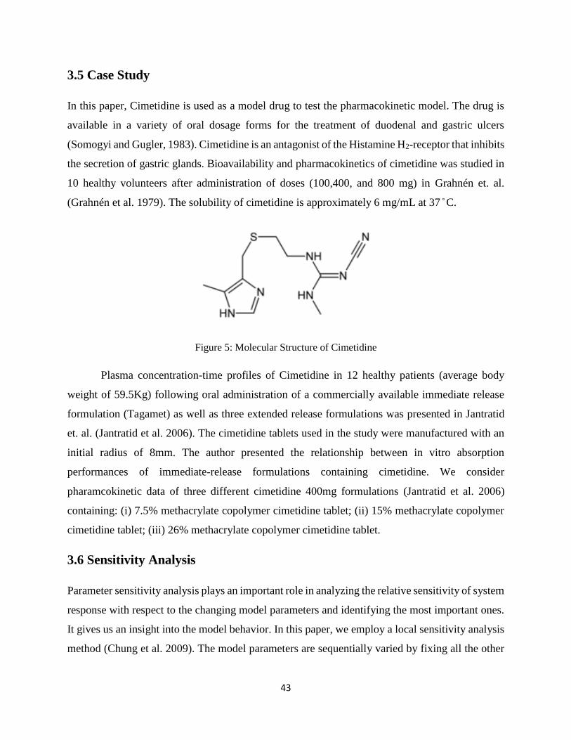
43

3.5 Case Study

In this paper, Cimetidine is used as a model drug to test the pharmacokinetic model. The drug is

available in a variety of oral dosage forms for the treatment of duodenal and gastric ulcers

(Somogyi and Gugler, 1983). Cimetidine is an antagonist of the Histamine H2-receptor that inhibits

the secretion of gastric glands. Bioavailability and pharmacokinetics of cimetidine was studied in

10 healthy volunteers after administration of doses (100,400, and 800 mg) in Grahnén et. al.

(Grahnén et al. 1979). The solubility of cimetidine is approximately 6 mg/mL at 37 ̊ C.

Figure 5: Molecular Structure of Cimetidine

Plasma concentration-time profiles of Cimetidine in 12 healthy patients (average body

weight of 59.5Kg) following oral administration of a commercially available immediate release

formulation (Tagamet) as well as three extended release formulations was presented in Jantratid

et. al. (Jantratid et al. 2006). The cimetidine tablets used in the study were manufactured with an

initial radius of 8mm. The author presented the relationship between in vitro absorption

performances of immediate-release formulations containing cimetidine. We consider

pharamcokinetic data of three different cimetidine 400mg formulations (Jantratid et al. 2006)

containing: (i) 7.5% methacrylate copolymer cimetidine tablet; (ii) 15% methacrylate copolymer

cimetidine tablet; (iii) 26% methacrylate copolymer cimetidine tablet.

3.6 Sensitivity Analysis

Parameter sensitivity analysis plays an important role in analyzing the relative sensitivity of system

response with respect to the changing model parameters and identifying the most important ones.

It gives us an insight into the model behavior. In this paper, we employ a local sensitivity analysis

method (Chung et al. 2009). The model parameters are sequentially varied by fixing all the other

44

parameters to their nominal values and the system response is determined. Normalized sensitivity

coefficient ( NSC ) values are evaluated from the values obtained using equation 4 (Chung et al.

2009). NSC values indicate the importance of a parameter on the system response.

(4)

Here is the nominal value of the system response at P0 the nominal value of the parameter;

similarly is the system response at P. The system response ( ) in this paper is evaluated as the

root mean squared error between the model and clinical data given by Eq. 5.

2mod exp

( ) ( )

1(5)

Nel

i i

i

C C

N

Here are plasma concentration values resulting from the model at selected time points (see

Appendix A and Appendix B). are the corresponding clinical values and N is the total number

of time points. We used a total of 16 time points in our model.

We performed sensitivity analysis for all the model parameters such as, human effective

permeability ( effP ), drug density ( d ), hepatic clearance rate of drug from the liver ( hCL ), volume

of liver ( liverV ), hepatic blood flow rate ( hQ ), volume of central compartment ( centralV ), diffusion

coefficient of water in polymer ( 1D ), diffusion coefficient of drug in polymer ( dD ), polymer chain

disentanglement rate ( dk ) and drug absorption scale factors ( i ). The effP value accounts for all

the factors responsible for the transport of drug across GI-epithelium such as passive transport as

well as active transport due to transporters. The hCL value accounts for the drug metabolism

happening inside the liver. The NSC values evaluated for five of the most sensitive parameters are

shown in Fig. 8. All the parameters are subjected to 2.5, 5, 7.5 and 10% perturbations on either

side of zero as shown in Fig. 6.

0 0

0 0

( ) /

( ) /NSC

P P P

0

C(i )

model

C(i )

exp

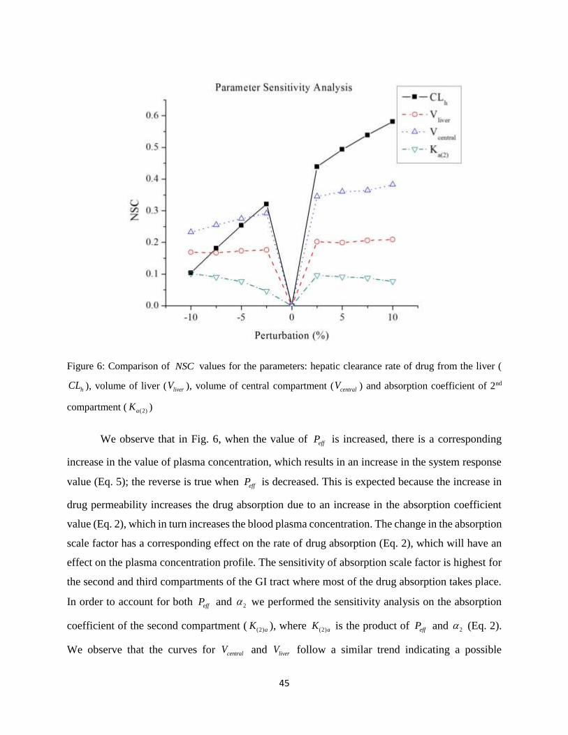
45

Figure 6: Comparison of NSC values for the parameters: hepatic clearance rate of drug from the liver (

hCL ), volume of liver ( liverV ), volume of central compartment ( centralV ) and absorption coefficient of 2nd

compartment ( (2)aK )

We observe that in Fig. 6, when the value of effP is increased, there is a corresponding

increase in the value of plasma concentration, which results in an increase in the system response

value (Eq. 5); the reverse is true when effP is decreased. This is expected because the increase in

drug permeability increases the drug absorption due to an increase in the absorption coefficient

value (Eq. 2), which in turn increases the blood plasma concentration. The change in the absorption

scale factor has a corresponding effect on the rate of drug absorption (Eq. 2), which will have an

effect on the plasma concentration profile. The sensitivity of absorption scale factor is highest for

the second and third compartments of the GI tract where most of the drug absorption takes place.

In order to account for both effP and 2 we performed the sensitivity analysis on the absorption

coefficient of the second compartment ( (2)aK ), where (2)aK is the product of effP and 2 (Eq. 2).

We observe that the curves for centralV and liverV follow a similar trend indicating a possible

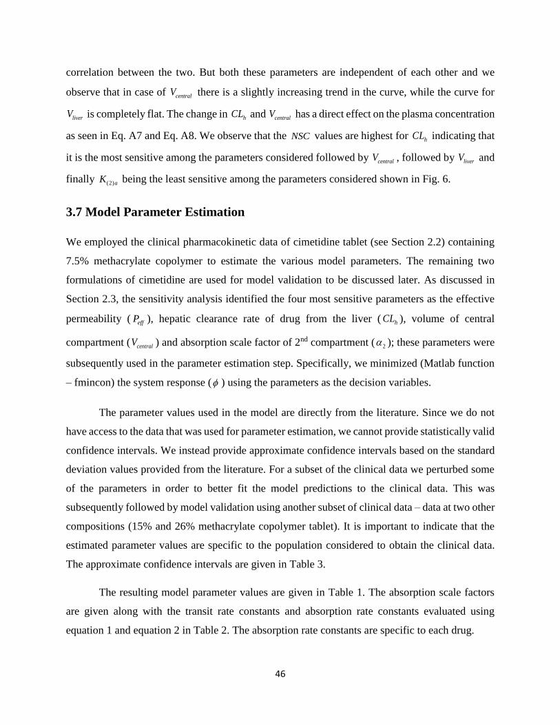
46

correlation between the two. But both these parameters are independent of each other and we

observe that in case of centralV there is a slightly increasing trend in the curve, while the curve for

liverV is completely flat. The change in hCL and centralV has a direct effect on the plasma concentration

as seen in Eq. A7 and Eq. A8. We observe that the NSC values are highest for hCL indicating that

it is the most sensitive among the parameters considered followed by centralV , followed by liverV and

finally (2)aK being the least sensitive among the parameters considered shown in Fig. 6.

3.7 Model Parameter Estimation

We employed the clinical pharmacokinetic data of cimetidine tablet (see Section 2.2) containing

7.5% methacrylate copolymer to estimate the various model parameters. The remaining two

formulations of cimetidine are used for model validation to be discussed later. As discussed in

Section 2.3, the sensitivity analysis identified the four most sensitive parameters as the effective

permeability ( effP ), hepatic clearance rate of drug from the liver ( hCL ), volume of central

compartment ( centralV ) and absorption scale factor of 2nd compartment ( 2 ); these parameters were

subsequently used in the parameter estimation step. Specifically, we minimized (Matlab function

– fmincon) the system response ( ) using the parameters as the decision variables.

The parameter values used in the model are directly from the literature. Since we do not

have access to the data that was used for parameter estimation, we cannot provide statistically valid

confidence intervals. We instead provide approximate confidence intervals based on the standard

deviation values provided from the literature. For a subset of the clinical data we perturbed some

of the parameters in order to better fit the model predictions to the clinical data. This was

subsequently followed by model validation using another subset of clinical data – data at two other

compositions (15% and 26% methacrylate copolymer tablet). It is important to indicate that the

estimated parameter values are specific to the population considered to obtain the clinical data.

The approximate confidence intervals are given in Table 3.

The resulting model parameter values are given in Table 1. The absorption scale factors

are given along with the transit rate constants and absorption rate constants evaluated using

equation 1 and equation 2 in Table 2. The absorption rate constants are specific to each drug.

47

Table 1: Model Parameters used in the developed pharmacokinetic model

Parameter Description Value Source

effP (cm/h) Human effective permeability of the drug

in the body

0.063 (Willmann et al. 2009)

d

(gm/cm3)

Density of the drug (cimetidine) 1.4 (Narasimhan and Peppas

1997)

liverV (ml) Volume of human liver 1539.6 (Agoram et al. 2001)

hQ

(ml/h/Kg)

Blood flow rate in the hepatic artery from

central compartment into the liver

1260 (Agoram et al. 2001)

hCL (ml/h) Hepatic clearance rate of the drug from the

liver

9036 (Gugler et al. 1982)

centralV (ml) Volume of central compartment 11900 (Gugle et al. 1982)

1D (cm2/s) Diffusion coefficient of water in polymer 2.5x10-

7

(Narasimhan and Peppas

1997)

dD (cm2/s) Diffusion coefficient of drug in polymer 2.2x10-

8


1997)

dk (cm/s) Disentanglement rate of polymer 3.3x10-

7


1997)

48

Table 2: Compartment parameters used in the modified ACAT model, absorption rate constants and transit

rate constants of each compartment

Compartment Compartmental

Absorption Scale

Factor

( i )

Compartment

Radius (cm)

Absorption

Rate

Constant

(h-1)

Compartment

Transit Time

(h)

Transit

Rate

Constant

(h-1)

1 2 9.67 0.13 0.25 4.00

2 10 1.53 4.12 0.26 3.85

3 10 1.45 4.34 0.93 1.07

4 4 1.29 1.95 0.74 1.35

5 2 1.13 1.11 0.58 1.72

6 2 0.98 1.29 0.42 2.38

7 2 0.82 1.54 0.29 3.45

8 2 3.39 0.37 4.19 0.24

9 2 2.41 0.52 12.57 0.08

Table 3: Standard deviation and 95% confidence interval values for the estimated parameters

Parameter Best-fit Value Standard Deviation 95% Confidence

Interval

effP (cm/h) 0.063 0.012 0.056 - 0.069

hCL (ml/h) 9036 2778 7523 – 10549

49

centralV (ml) 11900 6230 8506 – 15293

2 10 NA NA

3.8 Results and Discussion

We validated the model after estimating the model parameters. Specifically, we compared the

model data to the clinical data of the three different cimetidine formulations obtained from

Jantratid (Jantratid et al. 2006). We evaluated the pharmacokinetic metrics (process variables or

“parameters”) including the AUC, maxC and bioavailability and statistically compared them with

the model data.

We obtained clinical plasma concentration profiles for cimetidine 400mg tablet from

Jantratid (Jantratid et al. 2006) for three different formulations: (i) 7.5% methacrylate copolymer

cimetidine tablet (used in the parameter estimation); (ii) 15% methacrylate copolymer cimetidine

tablet and (iii) 26% methacrylate copolymer cimetidine tablet. Each formulation had an initial

dosage of 400mg containing excipients and 40% drug active. The clinical data indicates that the

plasma profiles are a function of the drug-polymer ratio in the tablet; hence the model is

constructed to reflect this ratio. The input mass for each of the three formulations is 1000mg, with

drug-polymer ratios 5.33, 2.66 and 1.54 respectively. We set the total simulation time as 12 hours.

The initial tablet radius was given as 8mm.

We estimated the error bars from the standard deviation values of maxC given by Jantratid

(Jantratid et al. 2006), where the only standard deviation given is that of maxC . From this standard

deviation value we tried to estimate the standard deviation for each point on the plasma profile.

Specifically, we assumed that the standard deviation was proportional to the concentration.

50

Figure 7: Comparison of model and clinical plasma concentration profiles for (a) 7.5% methacrylate

copolymer cimetidine tablet; (b) 15% methacrylate copolymer cimetidine tablet; (c) 26% methacrylate

copolymer cimetidine tablet, with estimated error bars for clinical plasma profiles. The experimental error

bars are estimated from the standard deviation values provided in the literature

We compared the clinical profile for each of the formulations with the predicted plasma

profile obtained from the model (Fig. 7). Fig. 7a shows the profiles for 7.5% methacrylate

copolymer cimetidine tablet, which is used as the basis for parameter estimation; hence the model

profile agrees well with the clinical profile with a low system response ( ) of 79.7 ng/ml evaluated

using Eq. 5. A low system response indicates that the root mean squared error between the model

predicted and clinical data is low. This implies that the model predicted data is quite close to the

clinical data indicating a good prediction by the model. In Fig. 7b, the predicted plasma profile for

(a)

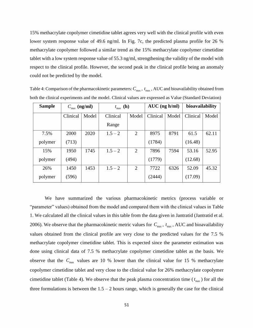
51

15% methacrylate copolymer cimetidine tablet agrees very well with the clinical profile with even

lower system response value of 49.6 ng/ml. In Fig. 7c, the predicted plasma profile for 26 %

methacrylate copolymer followed a similar trend as the 15% methacrylate copolymer cimetidine

tablet with a low system response value of 55.3 ng/ml, strengthening the validity of the model with

respect to the clinical profile. However, the second peak in the clinical profile being an anomaly

could not be predicted by the model.

Table 4: Comparison of the pharmacokinetic parameters: maxC , maxt , AUC and bioavailability obtained from

both the clinical experiments and the model. Clinical values are expressed as Value (Standard Deviation)

Sample maxC (ng/ml) maxt (h) AUC (ng h/ml) bioavailability

Clinical Model Clinical

Range

Model Clinical Model Clinical Model

7.5%

polymer

2000

(713)

2020 1.5 – 2 2 8975

(1784)

8791 61.5

(16.48)

62.11

15%

polymer

1950

(494)

1745 1.5 – 2 2 7896

(1779)

7594 53.16

(12.68)

52.95

26%

polymer

1450

(596)

1453 1.5 – 2 2 7722

(2444)

6326 52.09

(17.09)

45.32

We have summarized the various pharmacokinetic metrics (process variable or

“parameter” values) obtained from the model and compared them with the clinical values in Table

1. We calculated all the clinical values in this table from the data given in Jantratid (Jantratid et al.

2006). We observe that the pharmacokinetic metric values for maxC , maxt , AUC and bioavailability

values obtained from the clinical profile are very close to the predicted values for the 7.5 %

methacrylate copolymer cimetidine tablet. This is expected since the parameter estimation was

done using clinical data of 7.5 % methacrylate copolymer cimetidine tablet as the basis. We

observe that the maxC values are 10 % lower than the clinical value for 15 % methacrylate

copolymer cimetidine tablet and very close to the clinical value for 26% methacrylate copolymer

cimetidine tablet (Table 4). We observe that the peak plasma concentration time ( maxt ) for all the

three formulations is between the 1.5 – 2 hours range, which is generally the case for the clinical

52

values. We observe that the values of AUC predicted by the model are somewhat lower than that

evaluated from the experiments for the 15 % and 26 % formulations. The AUC value for 15 %

methacrylate copolymer cimetidine tablet is 3.8 % lower, while for 26 % methacrylate copolymer

cimetidine tablet it is 18 % lower as shown in Table 4. The large difference in the AUC values for

the 26% methacrylate copolymer cimetidine tablet is due to the unaccounted second peak in the

clinical profile (Fig. 7c). However, all the maxC and AUC values evaluated from the model still fall

within the clinical range of values given by Jantratid (Jantratid et al. 2006). We observe that the

bioavailability values evaluated from the model are comparable to the clinical values except for

the 26% methacrylate copolymer cimetidine tablet due to the large difference in AUC values.

3.9 Scenario Studies

We studied several scenarios by changing different inputs in the model and simulating their impact

on the plasma concentration profile. The analysis was done using the clinical data for 7.5%

methacrylate copolymer cimetidine tablet as the basis. Quantitative analysis was done by

comparing the AUC values for different input values in each of the scenarios. We determined the

optimal dimensions of drug tablet required for predicting a target plasma profile with maximum

efficacy.

3.9.1 Average body weight of a patient ( pW )

Plasma concentration profiles are simulated after increasing the body weight by 30, 70 and 100%

as shown in Fig. 6, along with the original predicted profile.

53

Figure 8: Comparison of model plasma profiles for different values of patient body weight

With an increase in the body weight, there is a significant negative shift in the plasma

profile from the original. That is the plasma profile shifts below the original profile due to an

increase in the parameter value as shown in Fig. 8. The negative shift is observed because, the

increase in the body results in an increase in the values of hepatic blood flow rate ( hQ ), volume of

central compartment ( centralV ) and hepatic clearance rate of drug from the liver ( hCL ), as all these

values are evaluated using the body weight. This shows that the developed model can be used for

different patients of different body weights. For patient body weight ( pW ) increase of 0%, 30%,

70% and 100% (AUC values of 8791, 8580, 8229 and 7936 ng.h/ml respectively), the decrease in

AUC values were 0%, 2.4%, 7.5% and 9.7% respectively. This low change in the AUC value

indicates low effect of pW on plasma concentration profile. We hypothesize that for a fixed drug

dosage, two patients of varying body weights are expected to experience similar therapeutic effect

of the drug.

54

3.9.2 Fraction of drug in polymer-drug system ( df )

Plasma concentration profiles are simulated after decreasing the fraction of the drug by 0, 20, 40

and 60 % as shown in Fig. 9. The total mass of the drug tablet was 1000 mg as mentioned before

containing 400 mg of drug.

Figure 9: Comparison of model plasma profiles for different values of fraction of drug ( df )

The decrease in the fraction of drug ( df ) is also an indication of the decrease in the drug

loading of the tablet. The mass of drug released (M) into the modified ACAT is directly

proportional to df as described by Eq. 3. Hence, the decrease in df will result in a corresponding

decrease in the value of M, which decreases the overall plasma profile. The plasma profile shifts

below the original profile due to decrease in the parameter value as shown in Fig. 9. The drug

loading of a tablet is a measure of the effectiveness of the drug tablet. Pharmaceutical scientists

thrive to produce drug formulations with maximum drug loading which could provide the most

effective therapeutic effect with minimum amount of drug dosage. For fraction of drug ( fd)

decrease of 0%, 20%, 40% and 60% (AUC values of 8791, 7030, 5276 and 3518 ng.h/ml

respectively), the AUC values correspondingly decreased by 0%, 20%, 40% and 60% respectively.

Thus fd

has a direct effect on the model predictions. We hypothesize that for a patient, the increase

55

in drug loading could lead to an overdose of the drug, and a decrease in drug loading could lead to

a very low or no therapeutic effect at all. Thus the dosage should be carefully tailored to the drug

loading of the tablet.

3.9.3 Tablet radius (R)

Plasma concentration profiles are plotted after increasing the tablet radius by 0, 20, 40 and 60% as

shown in Fig. 10. The mass of the tablet is kept constant. Hence, with increase in tablet radius,

there is a corresponding decrease in the tablet thickness.

Figure 10: Comparison of model plasma profiles for different values of tablet radius

An increase in the tablet radius has low to moderate impact on the plasma concentration

profile. There is a slight positive shift observed, with increase in the tablet radius (R). The mass of

drug released (M) into the modified ACAT model is dependent on this tradeoff between the R and

h values as described by Eq. 3. We observe that the overall effect on plasma profile is much less.

Thus one can determine the optimal tablet radius, which corresponds to an optimal tablet thickness

that has the maximum effect on the drug plasma profile. Most of the active drug is released in the

axial direction for a typical cylindrical tablet considered in our model. In this case the change in

the tablet radius will have a corresponding effect on the tablet surface area through which the axial

56

drug diffusion is taking place. This will have a significant impact on the drug release rate, which

directly impacts the plasma concentration profile. For the tablet radius (R) increase of 0%, 20%,

40% and 60% (AUC values of 8791, 10707, 11105 and 11605 ng.h/ml respectively), the AUC

values correspondingly increased by 0%, 22%, 26% and 32% respectively. This indicates that R

has a significant effect on the model predictions up to a certain percentage of increase; the effect

becomes low after that due to the tradeoff between R and h values as discussed above. Thus a tablet

with higher radius is expected to have a greater therapeutic effect compared to the one with a lower

radius, but risks crossing the toxicity threshold.

3.9.4 Optimization

In this scenario study, we consider tablet design before any experiments are performed. We are

trying to address the question, “What tablet geometry maximizes the therapeutic affect?” To

proceed, we make the assumption that the total volume of the tablet is constant and the overall

tablet composition (drug, polymer and excipients) is fixed. We also make the assumption that the

model parameters (such as permeability ( effP ), drug density ( d ), hepatic clearance rate of drug

from the liver ( hCL ), volume of liver ( liverV ), hepatic blood flow rate ( hQ ), volume of central

compartment ( centralV ), diffusion coefficient of water in polymer ( 1D ), diffusion coefficient of drug

in polymer ( dD ), polymer chain disentanglement rate ( dk ) and drug absorption scale factors ( i

).) do not change. We incorporated the developed pharmacokinetic model within an optimization

framework as described in Eq. 6 to determine the optimal tablet dimensions for a given drug

dosage. This will greatly help in determining drug tablet design, which will result in the maximum

therapeutic effect. In this model, we fixed the tablet size (volume) and tablet composition.

MinxJ = Performance Objective

subject to

PharmacokineticModel (6)

Here, J is the objective function, which in our case is the AUC value; x is the optimization variable,

which in this case is a tablet dimension. The pharmacokinetic model equations are defined by the

ACAT model, while the dissolution model equations are given in Appendices A and B. For the

15% methacrylate copolymer cimetidine tablet considered for this study with an initial radius of 8

57

mm, the optimal tablet radius is obtained as optR = 15.6 mm. This optimal value is obtained when

there are no constraints on the AUC value implying the maximum possible therapeutic effect. We

performed the optimization using the interior-point function “fmincon” in Matlab. We used an

Intel® Xeon(R) CPU E5405 2.00 GHz x 4 Processor; the simulation time was 37 minutes of CPU.

3.10 Conclusions

We have presented effective models for drug release, drug absorption and transit. The advantage

of the suggested approach is that it can be used to test hypothesis about the mechanism involved

in drug delivery into the blood circulatory system; these are issues we are exploring.

We concluded through parameter sensitivity analysis of the model that based on the NSC

values, effective permeability ( effP ) is the most sensitive, followed by absorption scale factor of

compartment 2 ( 2 ), hepatic clearance rate of drug from liver ( hCL ), volume of central

compartment ( centralV ) and volume of liver ( liverV ) in that order.

Using a set of parameter estimated values, we performed a comparative study of plasma

concentration profiles and pharmacokinetic metrics such as maxC , AUC and bioavailability between

model predictions and clinical data for three different cimetidine formulations, (i) 7.5%

methacrylate copolymer cimetidine tablet; (ii) 15% methacrylate copolymer cimetidine tablet; (iii)

26% methacrylate copolymer cimetidine tablet. The predicted plasma concentration profiles match

well with the clinical profiles for all the three cases. The estimated pharmacokinetic parameter

values of maxC , AUC and bioavailability fall well within the clinical range as given in Jantratid

(Jantratid et al. 2006).

We presented scenario studies, which showed that the developed model is applicable to

different patients with varying body weight ( pW ). It is also applicable to different drug tablets with

varying drug fraction ( df ) (or drug loading). We finally incorporated the model within an

optimization framework to estimate the optimal geometry of the tablet which will give the

maximum efficacy. The current model is limited to predicting the plasma concentration profiles

similar to that shown in Fig. 7 where most of the drug absorption takes place within the initial few

hours. We are extending the model to allow it to predict a plasma profile of a general shape.

58

This model is based on the ACAT model, which represents the GI tract as a series of well-

mixed continuous stirred tank vessels similar to continuous stirred tank reactors (CSTRs);

however, the GI tract is a continuous tube more closely represented by piece-wise tubular vessels

similar. In the one-dimensional case the tubular model is similar to a set of plug flow reactors

(PFRs). We are pursuing this angle as well with the understanding that higher model complexity

and model accuracy would result.

59

3.11 Nomenclature

( )i tk Transit rate constant for the ith compartment

( )i ak Absorption rate constant for the ith compartment

effP Effective permeability of drug in the body

i Drug absorption scale factor

it Transit time in each compartment of ACAT model

d Drug density

df Fraction of drug

L Initial half thickness of the drug tablet

0R Radius of the drug tablet

,kt ih Half thickness of the drug tablet at time kt in the ith compartment

1 ,kt ih

Half thickness of drug tablet at previous time point 1kt in the ith compartment

,com iV Compartment volume of the ith compartment

Nominal value of the system response

P0 Nominal value of the parameter; similarly

System response value

P Model parameter value

maxC Peak plasma concentration

maxt Peak plasma concentration time

Plasma concentration value on the model predicted curve at selected time points

Plasma concentration values on the clinical curve at selected time points

N Total number of time points considered to evaluate the system response

hCL Hepatic clearance rate of drug from the liver

liverV Volume of liver

hQ Hepatic blood flow rate

centralV Volume of central compartment

0

C(i )

model

C(i )

exp

60

1D Diffusion coefficient of water in polymer

dD Diffusion coefficient of drug in polymer

dk Polymer chain disentanglement rate

pW Average patient body weight

pC Plasma Concentration

61

3.12 References

Agoram, B., W. S. Woltosz and M. B. Bolger (2001). "Predicting the impact of physiological and

biochemical processes on oral drug bioavailability." Advanced Drug Delivery Reviews 50,

Supplement 1(0): S41-S67.

Bolger, M. B. (2009). "Simulations of absorption, metabolism, and bioavailability." Methods and

Principles in Medicinal Chemistry 40(drug bioavailability): 453.

Bolger, M. B. (2009). "Simulations of the Nonlinear Dose Dependence for Substrates of Influx

and Efflux Transporters in the Human Intestine." The AAPS Journal 11(2): 353-363.

Chung, S.-W., F. L. Miles, R. A. Sikes, C. R. Cooper, M. C. Farach-Carson and B. A. Ogunnaike

(2009). "Quantitative Modeling and Analysis of the Transforming Growth Factor ² Signaling

Pathway." Biophysical journal 96(5): 1733-1750.

Dokoumetzidis, A., L. Kalantzi and N. Fotaki (2007). "Predictive models for oral drug absorption:

from in silico methods to integrated dynamical models." Expert Opinion on Drug Metabolism &

Toxicology 3(4): 491-505.

Grahnén, A., C. Bahr, B. Lindström and A. Rosén (1979). "Bioavailability and pharmacokinetics

of cimetidine." European Journal of Clinical Pharmacology 16(5): 335-340.

Grass, G. M. (1997). "Simulation models to predict oral drug absorption from in vitro data."

Advanced Drug Delivery Reviews 23(1–3): 199-219.

Gugler, R., B. Muller-Liebenau and A. Somogyi (1982). "Altered disposition and availability of

cimetidine in liver cirrhotic patients." British Journal of Clinical Pharmacology 14(3): 421-430.

Huang, W., S. Lee and L. Yu (2009). "Mechanistic Approaches to Predicting Oral Drug

Absorption." The AAPS Journal 11(2): 217-224.

Jamei M, Y. J., Turner D, Rowland-Yeo K, Tucker GT, Rostami-Hodjegan A (2007). A Novel

Physiologically-Based Mechanistic Model for Predicting Oral Drug Absorption: The Advanced

Dissolution, Absorption, and Metabolism (ADAM) Model. . PKUK. Edinburgh Caledonian Hotel,

Edinburgh, UK.

62

Jantratid, E., S. Prakongpan, G. L. Amidon and J. B. Dressman (2006). "Feasibility of Biowaiver

Extension to Biopharmaceutics Classification System Class III Drug Products: Cimetidine."

Clinical Pharmacokinetics 45(4): 385-399.

Marshall, S., F. Macintyre, I. James, M. Krams and N. E. Jonsson (2006). "Role of

Mechanistically-Based Pharmacokinetic/Pharmacodynamic Models in Drug Development: A

Case Study of a Therapeutic Protein." Clinical Pharmacokinetics 45(2): 177-197.

Mehrotra, N., M. Gupta, A. Kovar and B. Meibohm (2006). "The role of pharmacokinetics and

pharmacodynamics in phosphodiesterase-5 inhibitor therapy." Int J Impot Res 19(3): 253-264.

Narasimhan, B. and N. A. Peppas (1997). "Molecular analysis of drug delivery systems controlled

by dissolution of the polymer carrier." Journal of Pharmaceutical Sciences 86(3): 297-304.

Ni, P. F., N. F. H. Ho, J. L. Fox, H. Leuenberger and W. I. Higuchi (1980). "Theoretical model

studies of intestinal drug absorption V. Non-steady-state fluid flow and absorption." International

Journal of Pharmaceutics 5(1): 33-47.

S. Darwich, A., S. Neuhoff, M. Jamei and A. Rostami-Hodjegan (2010). "Interplay of Metabolism

and Transport in Determining Oral Drug Absorption and Gut Wall Metabolism: A Simulation

Assessment Using the Advanced Dissolution, Absorption, Metabolism (ADAM) Model." Current

Drug Metabolism 11(9): 716-729.

van de Waterbeemd, H. and E. Gifford (2003). "ADMET in silico modelling: towards prediction

paradise?" Nat Rev Drug Discov 2(3): 192-204.

Willmann, S., A. Edginton and J. Dressman (2007). "Development and Validation of a Physiology-

based Model for the Prediction of Oral Absorption in Monkeys." Pharmaceutical Research 24(7):

1275-1282.

Willmann, S., A. N. Edginton, M. Kleine-Besten, E. Jantratid, K. Thelen and J. B. Dressman

(2009). "Whole-body physiologically based pharmacokinetic population modelling of oral drug

administration: inter-individual variability of cimetidine absorption." Journal of Pharmacy and

Pharmacology 61(7): 891-899.

63

Willmann, S., W. Schmitt, J. Keldenich and J. B. Dressman (2003). "A Physiologic Model for

Simulating Gastrointestinal Flow and Drug Absorption in Rats." Pharmaceutical Research 20(11):

1766-1771.

Willmann, S., W. Schmitt, J. Keldenich, J. Lippert and J. B. Dressman (2004). "A Physiological

Model for the Estimation of the Fraction Dose Absorbed in Humans." Journal of Medicinal

Chemistry 47(16): 4022-4031.

Yu, L. X. and G. L. Amidon (1999). "A compartmental absorption and transit model for estimating

oral drug absorption." International Journal of Pharmaceutics 186(2): 119-125.

Yu, L. X., E. Lipka, J. R. Crison and G. L. Amidon (1996). "Transport approaches to the

biopharmaceutical design of oral drug delivery systems: prediction of intestinal absorption."


64

3.13 Appendix A

3.13.1 ACAT Model

According to the ACAT model, the rate of change of dissolved drug concentration in a GI

compartment depends on:

1. Release of drug from the formulation into the compartment

2. Transit of drug into a compartment

3. Transit of rug out of a compartment

4. Absorption/exsorption of the drug

The model equations are given by:

Nomenclature

Superscript Subscript

Dissolved – 1 t – Transit

Absorbed – 2 a – Absorption

Stomach

The stomach is treated as another compartment (Compartment 1). Notes: (a) in Eqn. (A.1), carrier-

mediated transport is ignored; (b) in Eqn. (A.2), gut metabolism is ignored; (c) level 2 is

“enterocyte” (level 2).

Small Intestine

The small intestine is divided into 7 compartments from (i = 2 to 8) and, i = 9 is the colon. The

general equations for each of the compartments with different forms of the drug are given below

(assumes lateral and vertical transit coefficients have same values).

(1)(1) (1) (1) (1) (2)1

1 1 0 1 1 1

(2)(1) (1) (2) '(2) (2) (2) (2)11 1 1 1 1 1 1

(1) (2)

1 1

( ) ( .1)

( ) ( ) ( .2)

: (0) (0) 0

feed t a

a a p t

dCC k C k C C A

dt

dCk C C k C C k C A

dt

Initial Cond C C

65

Notes: (a) in Eqn. (A.3), carrier-mediated transport is ignored; (b) in Eqn. (A.4), gut metabolism

is ignored; (c) level 2 is “enterocyte” (level 2).

Portal Vein (i.e. Plasma)

The rate of absorption of drug into the portal vein is given by:

This absorbed drug from the portal vein mixes with some of the recycled drug from the central

compartment before it goes into the liver for first pass extraction. The mixing equation is given

by:

, ( .6)absliver in p

H

RC C A

Q

Liver

The drug undergoes first pass elimination in the liver and the model equation is given by:

Central Compartment

The final plasma drug concentration ( pC ) is measured in the central compartment and the model

equation is given by:

(1)(1) (1) (1) (1) (1) (1) (2)

( 1) ( 1)

(2)(1) (1) (2) (2) (2) '(2) (2) (2) (2)

( 1) ( 1)

( )

'( )

( ) ( .3)

( ) ( ) ( .4)

: (0) 0 2,...,9

iifeed i t i it i ia i i

iia i i i t i ia i p it i

j

i

j

ia

dCC k C k C k C C A

dt

dCk C C k C k C C k C A

dt

Initial Cond C i

Assume k

( )j

iak

9'(2) (2)

,

1

( ) ( .5)Abs com i ia i p

i

R V k C C A

,( .7)

(0) 0

liver in H liver h liver Hliver

liver

liver

C Q C CL C QdCA

dt V

C

66

The various properties of compartments in the ACAT model such as the compartment volume,

radius and length of each compartment, transit time in each compartment and the pH conditions in

each compartment are given in Table A.1.

Table A.1: ACAT model compartment parameters for fasted human physiology (Bolger 2009)

Compartment Volume (mL) Radius (cm) Length (cm) Transit time

(h)

pH

Stomach 47 9.67 28.3 0.25 1.3

Duodenum 42 1.53 14.1 0.26 6.0

Jejunum 1 154 1.45 58.4 0.93 6.2

Jejunum 2 122 1.29 58.4 0.74 6.4

Ileum 1 94 1.13 58.4 0.58 6.6

Ileum 2 71 0.98 58.4 0.42 6.9

Ileum 3 49 0.82 58.4 0.29 7.4

Caecum 47 3.39 13.2 4.19 6.4

Colon 50 2.41 27.6 12.57 6.8

( .8)liver H p Hp

central

C Q C QdCA

dt V

67

CHAPTER 4

Identifying polymer structures for oral drug delivery – a molecular

design approach

Abstract

A computer aided molecular design (CAMD) approach is proposed for generating molecular

structures of polymer candidates which have the potential to be effective polymer carriers in drug

delivery. A group contribution method has been used to predict properties such as glass transition

temperature (gT ), expansion coefficient (

f ) and water absorption (W ). A mixed integer

nonlinear optimization technique was used to successfully generate some novel polymer structures

not available in the literature. The generated polymers have been ranked according to a desirability

curve. A solubility parameter analysis was done to further analyze and filter the generated

polymers. The proposed new polymers need further investigation to be practically useful in oral

drug delivery.

Keywords: oral drug delivery; molecular design; structure - property models; novel polymers;

optimization


In this chapter, we propose a computer aided molecular design (CAMD) approach to generate

molecular structures of polymer candidates with desired properties. This work is aimed towards

drug product development process, where our focus lies in the development of novel polymers that

can be used as potential carrier materials for drugs in drug delivery applications.

68

Figure 1: CAMD approach in product development process

To address the problem as stated above, we employ structure-property models, specifically

group contributions to predict properties such as glass transition temperature ( gT ), expansion

coefficient ( f ) and water absorption (W ). We then employ a mixed integer nonlinear

optimization model to successfully generate molecular structures of novel polymers along with

their properties. This approach can significantly reduce the number of laboratory experiments

involved in the product development process by identifying a few viable candidates for

development (Fig. 1).


Polymers have a large impact on our everyday life because of their wide range of applications.

Plastics, textiles and rubbers are the most common polymers with extensive use in the society. By

convention all the polymers are designed through laboratory scale experiments using trial-and-

error techniques. However it is inefficient to completely rely on experimental synthesis and testing

of many alternatives, since the number of possibilities can be combinatorially large. Computational

polymer molecular design can help in the screening of polymer structures, which can then be

followed by laboratory scale experiments. This is economical and less time consuming.

69

The chemical industry is designing new polymers with desired functional properties for

different applications. One such application is in the pharmaceutical industry, where a drug is to

be encapsulated inside a polymer matrix to aid in oral drug delivery. For example the drug is to be

protected from the various influences in the GI tract. There are several factors in the GI tract which

may limit the absorption and solubility of the drug in the intestine; examples are the morphological

barriers (mucus layer, micro villi, etc.), chemical barriers (acids, bicarbonates, etc.) and

physiological barriers (a wide range of pH, enzymatic activities, specific transport mechanisms,

etc.) (Gaucher et al. 2010). Therefore, the dissolution of a drug is quite often, the rate-limiting step,

which ultimately controls the bioavailability of the drug. Polymers can be used as drug carriers

because the chemical groups present in the structure can firmly bind with the drug and form an

amorphous matrix. Polymers aid in targeted drug release in the small intestine where maximum

absorption takes place.

4.2.1 Polymers in Oral Drug Delivery

Biodegradable polymers are defined as polymers which degrade in vitro and in vivo either into

products that are normal metabolites of the body or into products that can be completely eliminated

from the body with or without further metabolic transformation. The degradation products should

be nontoxic, and that the rate of degradation and mechanical properties of the material should

match the intended application. Nondegradable hydrophobic polymers initially used for drug

delivery applications such as poly(dimethylsiloxane) (PS), polyurethanes (PU), and poly(ethylene-

co-vinyl acetate) (EVA) (Mathiowitz 1999) were not suitable for in-vivo applications due to the

need to remove them. Since biodegradable polymers do not have to be removed after delivery,

they are preferred vehicles for drug delivery applications. The release of drugs is favored by

bioerosion of polymer matrices. Thus, both natural and synthetic biodegradable polymers have

been extensively investigated for drug delivery applications.

Natural polymers are mostly chosen due to their excellent biocompatibility, as structurally

they closely mimic native cellular environments, have unique mechanical properties, and are

biodegradable by an enzymatic or hydrolytic mechanism. However, they have certain inherent

disadvantages associated with some of them such as risk of viral infection, antigenicity, unstable

material supply, and batch-to-batch variation in properties (Barbucci 2002). Synthetic polymers,

on the other hand, offer tremendous advantages over natural polymers from the material side. Due

70

to their synthetic flexibility it is possible to develop polymers having a wide spectrum of properties

with excellent reproducibility. Furthermore, fine-controlling of the degradation rate of these

polymers is highly feasible by varying their structure. The section below discusses the applications

synthetic and natural biodegradable polymers in drug delivery.

4.2.2 Synthetic Biodegradable Polymers

In controlled drug delivery it is desirable to deliver a biologically active molecule for a desired

time period and rate in order to maintain the drug level in the body within the therapeutic window.

Synthetic biodegradable polymers have shown great promise in controlled drug delivery. The

polymers are used as a matrix from where the drugs will released in a controlled manner. The rate

of release of drugs from a matrix depends on several parameters such as nature of the polymer

matrix, matrix geometry, properties of the drug, initial drug loading, and drug–matrix interaction

(Bae YH 1998, Mathiowitz 1999, Hamdy Abdelkader 2008, Phaechamud 2008). The release of

the drug from the polymer matrix can be by (i) a physical mechanism such as diffusion, (ii) solvent

controlled or chemical mechanism such as by dispersion or (iii) conjugating drugs in the

biodegradable polymer matrix. Several studies have been done to optimize parameters resulting in

desired drug release profiles from polymeric matrices.

In case of synthetic biodegradable polymer, the drug release for the polymer matrices can

be tuned by controlling the rate of degradation of the polymers by varying the nature and ratios of

monomeric units. The biodegradable polymers can be used to form hydrogels. The most important

biodegradable polymers for drug delivery applications are aliphatic polyesters such as PLA, PGA,

and their copolymers (PLAGA) (Vert et al. 1998, Jain et al. 2011). Initally, monolithic

formulations of these formulatios were studied where two-dimensional matrices of suitable

geometry were prepared by casting an organic solution of polymer and drug followed by solvent

evaporation or by compression/injection molding. Studies were performed to release cyclazocine

from PLA implants. Among these, PLAGA became the most suitable polymer for drug delivery

due to the ease of property manipulation possible with this polymer (Lewis 1990, Mathiowitz

1999). PEG (Bezemer et al. 2000) and poly (ester carbonates) (Nair and Laurencin 2006) are used

as drug delivery systems. Hydrophobic polymers poly(ortho esters) are used treatment of

postsurgical pain and ophthalmic diseases. Another aliphatic polyester that assumes importance

71

as a drug delivery matrix is poly(caprolactone) (PCL). Poly(caprolactone) (PCL) is a

semicrystalline polyester, with a melting temperature around 55–60°C and a Tg of – 60ºC. PCL is

highly soluble in organic solvents, has low melting point and Tg. It has an exceptional ability to

form blends with a variety of polymers. It has a low degradation rate. Capronor, is the

commercially available long-term contraceptive device based on PCL which releases

levonorgestrel following zero order kinetics (Ueda 2003). It has low degradation rate and higher

permeability of drugs compared to PLAGA. It has been extensively investigated drug delivery

applications (Blanco et al. 2003, Magdalena M. Stevanović 2007, Cynthia D’Avila Carvalho

Erbetta 2012). Poly(ortho esters) and polyanhydrides were developed as matrices for drug delivery

to achieve zero-order release kinetics (Mathiowitz 1999, Attawia et al. 2001, Chiu Li et al. 2002,

Heller et al. 2002).

Several other biodegradable polymer systems investigated as drug delivery matrices

include polyphosphazenes (Lakshmi et al. 2003), polyphosphoesters (Zhao et al. 2003),

poly(amino acids) , poly(alkyl cyanoacrylates) (Harmia et al. 1986, Nicolas and Couvreur 2009,

Dossi et al. 2010), polyhydroxy alkanoates (Kassab et al. 1997, Shrivastav 2013) and

poly(glutamic acid) (Li 1998, Yuan et al. 2010).

Langer et al. proposed polyanhydrides to be ideal candidates for drug delivery applications

(Rosen et al. 1983, Jain et al. 2008). Poly[(carboxy phenoxy)propane-sebacic acid] (PCPP-SA) is

a class of polyanhydride approved by FDA as a delivery matrix for the controlled delivery of the

chemotherapeutic agent BCNU to treat brain cancer under the trade name Gliadel.

Poly amino acids like tyrosine-derived polycarbonates are hydrophobic amorphous

polymers with Tg less than 100 ºC and decomposition temperatures around 300 ºC (Ertel and Kohn

1994). Tyrosine carbonates (desaminotyrosyl-tyrosine alkyl esters, DTH) has been investigated

for delivering dopamine drug as the polymer has similar structure to the drug and slow degradation

rate. Biodegradable polyphosphazenes are now being extensively investigated as matrices for drug

delivery applications, particularly protein delivery (Andrianov and Payne 1998, Lakshmi et al.

2003, Brüggemann 2013). Polyphosphoesters are currently being investigated as nerve conduits

and as matrices for drug and gene delivery applications (Zhao et al. 2003). Poly(lactide-co-ethyl

phosphate) matrices were used for delivery of chemotherapeutic drugs such as paclitaxol. They

72

showed zero order release and now under clinical trials under the trade name PACLIMER (Zhao

et al. 2003).

4.2.3 Natural Biodegradable Polymers

Polysaccharides such as cellulose derivatives are important matrices for drug delivery applications

(Swarbrick 1991, Robert 2006). Starch has several applications as drug delivery systems. A slow-

release drug delivery system based on amylose-rich starch under the trade name Contramid is

available in the market. Starch microspheres have been used as a bioadhesive drug delivery system

for the nasal delivery of proteins (Illum, Fisher et al. 2001). Alginate hydrogels have shown

potential as drug delivery systems (Mumper 1994, Tønnesen 2002, Izawa 2013). Alginate beads

are employed for the controlled delivery of many cationic drugs and various growth factors. The

drug loading and rate of release from these systems is greatly influenced by the ionic interaction

between the drug and the alginate matrix. Polyelectrolyte complexes of alginate with other cationic

polymers such as chitosan have been extensively investigated for cell encapsulation or as drug

delivery matrices. Cross-linked chitosan hydrogel are attractive materials for controlling drug

delivery by varying the cross-linking density. Other drug delivery systems include proteins, gelatin

complexes etc.

Polyhydroxyalkanoates (PHA) are biocompatible, processable, and degradable and hence

used as matrices for drug delivery applications (Kassab et al. 1997, Ueda 2003, Shrivastav 2013).

Poly(γ-glutamic acid) (γ-PGA) was used to deliver a novel drug delivery system to deliver

anticancer drug Taxol (Li 1998). The hydrogels of poly(glutamic acid) prepared by γ-irradiation

are under investigation as drug delivery matrices (Choi 1995).

Synthetic and natural biodegradable polymers have huge impact as controlled drug delivery

systems. However, investigation of more novel and functionalized polymers are required. The

future development of biodegradable polymeric biomaterials will consider appropriate physical,

mechanical, biological and degradation properties.

The rest of the manuscript is organized as follows. In section 4.3, we discuss some of the

well-known property prediction methods available in our arsenal. Section 4.4 describes the

computational method used to solve the CAMD problem. In section 4.5, the various aspects

considered in developing the CAMD problem are discussed, such as the properties of the polymer

73

and the problem formulation. Section 4.6 includes the results and discussion followed by

conclusions in section 4.7.

4.3 Polymer Property Prediction

A polymer is a macromolecule consisting of identical repeat units (monomers), which are linked

by covalent bonds. A polymer containing identical repeat units is called a homo-polymer. The

design of a polymer repeat unit requires the ability to estimate the physico-chemical properties of

the repeat unit and by extension the polymer itself. There are several property prediction models,

some of which are geared toward thermodynamic properties, whereas some are geared towards

transport properties. We have employed a computer aided molecular design (CAMD) framework

for the design of the repeat unit in a homo-polymer. Specifically desired property targets are to be

achieved. In the literature there has been a significant amount of effort on the design of homo-

polymer repeat units using CAMD (Venkatasubramanian 1994, Maranas 1996, Camarda and

Maranas 1999). The authors used property models to estimate the properties of generated repeat

units, which were then screened, based on the desired property constraints.

The accuracy of CAMD methodologies are dependent on the accuracy of the property

prediction models. There are two types of property prediction methods, reference methods and

approximate methods. Reference methods are generally used to verify or validate a theory. While

approximate methods are developed by fitting them to an experimental data and try to match the

proposed theory in a limited range (Gani and Constantinou 1996). Hence, the approximate methods

are computationally inexpensive but less reliable while the reference methods are computationally

intense but more reliable. Some of the reference methods known as mechanical methods are

discussed below. Approximate methods are subcategorized into empirical and semi-empirical

methods.

4.3.1 Molecular Modeling

Molecular mechanics, molecular dynamics and quantum mechanics are some of the well-known

mechanical models. Some of the molecular properties such as electrostatic potentials or

polarizability are accurately obtained using Quantum mechanics techniques (Gasteiger and Engel

2003). The calculations involved in Quantum mechanics are complex and slow because the

74

electrons are treated explicitly. On the other hand molecular mechanics treats electrons implicitly,

which makes the calculations much faster than quantum mechanics. Most of the static properties

are estimated using molecular dynamic (MD) techniques. Dynamic properties such as viscosity

can be estimated using non-equilibrium MD. All the above methods can be used to simultaneously

determine the molecular properties and their structure. However, the computational effort involved

means that they cannot be used explicitly within a CAMD framework, unless an off-line mode of

use is considered.

4.3.2 Empirical and Semi-Empirical Models

Empirical models are models developed based solely on the experimental observations. Some of

the well-known empirical models are chemometrics (Timmerman 2008), quantitative structure

activity relationship (QSAR) (Esposito 2004), and pattern matching and factor analysis (Wolber

2008). These models are more suitable to study known processes rather than new ones (Gani and

Constantinou 1996). Hence, these models are not very applicable in CAMD based polymer design.

Semi-empirical models are developed partly on theoretical concepts and partly on observations

and are widely used by scientists for property estimation (Van Krevelen 1990).

Some of the most commonly known semi-empirical models are corresponding states

models (Sola et al. 2008), topology or geometry based models (Moore and Peters 2005), models

based on additivity of groups, atoms or bonds and hybrid methods, which is integration of two or

more of the above models (Venkatasubramanian 1994). The group additivity and topology or

geometry models are used quite often employed in CAMD algorithms (Derringer and Markham

1985, Venkatasubramanian 1995, Camarda and Maranas 1999). The following sub sections will

give a brief theoretical description of the methods used in this work.

4.3.3 Group / Atom / Bond Additivity

Atom, group or bond additivity methods are used for estimating a property of a molecule based on

the assumption that the interactions between atom or groups or bonds in a molecule or polymer

are effective only within a short range. The property of a molecule using the additive atom or group

or bond contribution method is given by Eq. (1).

75

( ) (1)N

i

i

F Y m p

Y is the property estimated, ip corresponds to contribution of atom or group or bond, i , and m

corresponds to the number of occurrences of atom or group or bond in a chemical structure. The

group additive approach is widely used among these three additive methods. In a group

contribution method, the contribution of an individual group is independent of the molecule in

which the group occurs. Some of the major contributions in the area of group additivity based

property estimation methods is by (Van Krevelen 1990, Gani and Constantinou 1996, Marrero and

Gani 2001).

In the method by Marreo and Gani, the molecular structure of a compound is represented

as a collection of three types of groups: first-order, second-order and third-order. The first-order

groups are used to describe the whole molecular structures while the second- and third-order

groups are used to provide more structural information of the molecular fragments (Marrero and

Gani 2001). The method for estimating a property, Y, is given by Eq. 2.

( ) (2)i i j j k k

i j k

f Y N C w M D z O E

where, iC is the contribution of first-order group of type-i that occurs

iN times, jD and kE are the

contributions of second-order groups of type- j and third-order groups of type- k , that occur jM

and kO times, respectively. ( )f Y is a simple function of the property Y .

Van Krevlen (Van Krevelen 1990) proposed a simple group contribution method for

estimating the properties from the homo-polymer repeat unit structures. These property models are

quite accurate and have been used widely in different CAMD based applications (Derringer and

Markham 1985, Venkatasubramanian 1995).

Property estimation methods based on topological information related to molecular

structures commonly use connectivity indices (Kier and Hall 1986, Bicerano 2002). Application

of this approach is well known for the estimation of physicochemical properties such as boiling

point, partition coefficients, molar refraction, solubilities and many more (Randić 2001). Bicerano

(Bicerano 2002) developed property models for estimating polymer properties from the polymer

76

repeat-unit structures using connectivity indices. A large range of properties can be estimated using

this methodology.

4.4 Computational Techniques in Computer Aided Molecular Design

A computational technique is generally used in a CAMD algorithm to find a desired set of feasible

chemical structures by generating and evaluating various alternatives. A set of structural and

property constraints are used to identify the set of chemically feasible molecular structures that

satisfy the design specifications. The generation of a wide range of feasible molecular structures

and reliable property estimation of the generated molecular structures are the limiting steps in any

CAMD based technique (Churi and Achenie 1996, Duvedi and Achenie 1996, Harper 1999,

Karunanithi 2005, Karunanithi 2006).

In a Mathematical optimization technique the CAMD problem is formulated into an

optimization problem. Here, the property constraints are formulated as mathematical constraints

and the objective function is based on the performance criteria weighting the property values into

a single score. Minimizing the objective function solves the optimization problem. A Mixed

Integer Non Linear Programming (MINLP) method is commonly employed to solve the

optimization problems encountered in CAMD. Application of an MINLP solution technique has

disadvantage of (potentially) high computational cost and (potential) difficulties in finding the

global optimum (Ostrovsky et al. 2002, Karunanithi 2005, Karunanithi 2006).

4.5 CAMD Model Development – Polymers as Drug Carriers

This section provides a detailed description of the various factors considered in developing the

CAMD model. The first factor that is considered is identifying and studying the effect of various

polymer properties on the rate of release of the drug from the polymer matrix. A detailed

description of the problem formulation and the techniques used to solve the problem are discussed.

77

4.5.1 Properties of Polymers as Drug Carriers

There are several polymer properties that influence the rate of drug release from a polymer matrix

enclosed drug system. Some of the most important properties are described below.

Glass Transition Temperature ( gT ): Glass transition temperature is the temperature at which a

polymer changes from a glassy state (hard and brittle) to a rubbery state (soft and flexible). It is

defined for some crystalline as well as amorphous polymers. The gT of a polymer is also a measure

of the free volume within the polymer. The higher the free volume of the polymer, the lower the

gT and lower free volume implies a higher gT (Jadhav 2009). For the polymer to be used as a drug

carrier, it should be very stable (in glassy state) outside the body and transform into the rubbery

state while inside the body to give a better release of the drug. The gT is expected to be greater

than the body temperature (37 ºC).

Molecular weight: Increase in molecular weight leads to decrease in chain end concentration.

Higher molecular weight implies a bulkier polymer having a lower free volume, implying a higher

gT .

Expansion Coefficient ( f ): Higher expansion coefficient of polymer implies greater flexibility

when it is in its rubbery state inside the GI tract. And greater the expansion, higher the rate of drug

release from the polymer matrix.

Water absorption (W ): Increase in moisture content leads to increase in free volume due to

formation of hydrogen bonds with polymeric chains increasing the distance between polymeric

chains (Jadhav 2009). The increased free volume between polymeric chains result in decreased

Tg. Simultaneously, low hydrogen bonding between drug and polymer provides more hydrogen

bonding sites for water molecules resulting in decreased physical stability.

pH: pH of the polymer plays a major role especially when the polymer is pH sensitive. Depending

on the pH of the environment, the polymer will either swell or collapse. For polymers containing

acidic groups such as –COOH, -SO3H, it will swell at basic pH (higher pH), which makes it quite

stable under acidic conditions inside the stomach. For polymers containing basic groups such as –

NH2, it will swell in acidic pH and hence making it unstable in the stomach.

78

Solubility: If the polymer is highly soluble in water, implying that it has hydrophilic groups in its

molecular structure and hence will lead to a higher and faster release of drug. But a high solubility

leads to instability in the aqueous medium or inside the GI system. If the polymer contains

hydrophobic groups, it is more stable water but poorly soluble and gives a low release of drug.

Hence, there is always a tradeoff between the release rate of drug and stability of the polymer

based on the solubility.

Pore Size: Higher the pore size or porosity of the polymer, greater the amount of moisture it could

absorb leading to a higher drug release rate.

Chemical Groups: Polymers having bulky groups in its structure are less flexible. Bulky groups

lead to decrease in the free volume of the polymer, which results in a higher gT . Higher gT leads

to lower drug release as discussed above. Having long side groups in the structure makes the

polymer chains move apart from each other leading to an increase in the free volume. A higher

free volume implies a higher drug release. Presence of polar groups in the molecule will lead to

increase in the intermolecular forces, attraction within chains and cohesion. This will bring the

molecules much closer leading to a lower free volume.

4.5.2 Problem Formulation

A step by step description of the CAMD problem formulation are described as given in Table 1

Table 1: Step by step procedure for formulating a CAMD problem

Step 1 Choose a basis set of groups which could be in the desired polymer repeat-unit

Step 2 Define structural constraints (min. and max. number of groups in the repeat-unit)

Step 3 Define desired property constraints using structure-property models and group

contributions

Step 4 Solve Mixed-Integer Nonlinear Optimization Model to obtain repeat units satisfying

the constraints from Step 2 and Step 3

According to step 1, the basis set of groups is determined by choosing the most probable

groups which could be present in the polymer repeat unit. This is a result of determining all the

groups which are present in the molecular structures of polymers currently being used as oral drug

79

carriers. Table A1 in the appendix gives a list of polymers which we have used to determine the

groups and also the groups extracted from each of the polymers, resulting in the basis group set

given in Table 2.

Table 2: Basis group set and the respective contributions for different properties

S. No Group Valence

(iv )

Molecular

weight

(iM )

(gm/mol)

Molar glass

transition function

(giY )

(gm.K/mol)

Molar

volume

(giV )

(cm3/mol)

Molar water

content

(iH )

(gm(water)

/mol)

1 3CH 1 15 8121.78 35.5 0

2 2CH 2 14 2361.26 16.1 3.3E-5

3 CH 3 13 987.78 -1 0

4 C 4 12 0 -19.2 0

5 CH CH 2 26 5976.32 27 0

6 SiO 2 44 -18917.29 3.8 0.02

7 COO 2 44 21739.93 18 0.075

8 OH 1 17 17433.54 10 0.75

9 CHCl 2 48.5 19388.75 25 0.015

10 CONH 2 43 30748.83 9.5 0.75

11 2CH O 2 30 5834.32 19.9 0.02

12 2CH COO 2 58 15447.25 34.1 0.075

13 N 3 14 -31461.27 5 0

14 CCN 3 38 15883.2 4.8 0.065

15 CHCN 2 39 17695.43 23 0.065

16 2CONHCH 2 57 23529.58 25.6 0.75

17 CHCOO 3 57 11629.78 17 0.075

18 2CH NH 2 29 33150.95 20.6 0.64

19 CHO 3 29 2250.41 22.3 0.02

80

20 2CH CO 2 42 13169.56 26.9 0.11

According to step 2, the structural constraints include the minimum (minn ) and maximum (

maxn ) number of groups, which could be present in the repeat unit given by Eq. (3). They include

the valence constraint, which is the total valence of the polymer repeat unit defined using Eq. (4).

The structural constraints make sure that the molecules obtained are physically realizable.

min max (3)i

i

n n n

(2 ) 2( 1) (4)i i

i

v n k

where, in and

iv are the number and valence, respectively, of the groups of type i ; k in the

equation takes the value of 1, 0 or -1 depending on the type of structures formed, namely acyclic,

monocyclic and bicyclic. In our work, we concentrated on acyclic structures.

According to step 3, property constraints define the desired limits for property values and

are given by Eq. (5). These properties are estimated using correlations and structure-property

models such as group contributions.

( ) (5)l i uP P n P

where, lP and

uP are the lower and upper bounds of the properties specified for a polymer repeat

unit structure and ( )iP n is the predicted property value. In this work, three different properties are

considered, namely, glass transition temperature (gT ), expansion coefficient (

f ) and water

absorption (W ) are estimated using Eq. (6).

180.115(6)

gi i

g f

i g i

Y HT W

M T M

where, iH ,

iM and giY represent the group contributions for molar water content, gram molecular

weight and molar glass transition function respectively.

81

Finally in step 4, we solve the formulated problem using a computer aided technique such

as mixed-integer nonlinear optimization to generate the molecular structures of repeat units

satisfying the constraints defined in step 2 and step 3. The CAMD optimization problem can be

expressed as given in Eq. (7).

min ( ) (7)

s.t.

0 (8)

( ) 0 (9)

integer

f x

Ax b

g x

x

where, the linear constraints comprise of the structural constraints given by Eq. (8), and the

nonlinear constraints comprise of the valence and property constraints given by Eq. (9). The

performance objective function ( ( )f x ) can be in different forms. In this work we used a

desirability function for glass transition temperature (gT ) as the objective function and is given by

Eq. (10).

( ) 1 ( ) (10)

where,

(11)

(12)

i

sl

li ii i il

i i

i tu

ui ii i iu

i i

f x d x

Y YY Y c

c Yd

Y Yc Y Y

c Y

where, iY is the predicted property value, u

iY and l

iY are the upper and lower bounds of the

property, ic is the most desirable value of the property, which corresponds to a desirability of 1.

The values of s and t determine the rate at which the property is changing above and below ic .

4.5.3 Mixed Integer Nonlinear Optimization – Outer Approximation Algorithm

The mixed integer nonlinear optimization problem discussed in step 4 is solved using a generalized

outer approximation (GOA) algorithm. The algorithm involves successive solutions of nonlinear

programs (NLP’s) and mixed integer linear programs (MILP’s). Here, each iteration generates an

82

upper and lower bound on the MINLP solution. A general form of the optimization problem is

given by Eq. (13) (Floudas 1995).

,min ( , )

. . ( , ) 0 (13)

x yf x y

s t g x y

x R y Z

In the first step, a resulting primal problem 1( )P y is solved for an initial value of 1y and

the obtained solution is denoted by 1x . The primal problem is given by Eq. (14) is an NLP. The

current upper bound is set as 1( )UBD P y .

1

,

1

min ( , )

. . ( , ) 0 (14)

x yf x y

s t g x y

x R

In the second step, the relaxed master problem given by Eq. (15), is solved. The relaxed

master problem is an MILP. The solution to the relaxed master is given by 1ky and k at a general

iteration step k.

, ,min

. . ( , ) ( , ) (15)

0 ( , ) ( , )

x y

k

k k k k T

k

k

k k k k T

k

x xs t f x y f x y

y y

x xg x y g x y

y y

x R y Z

where, kx is the feasible solution to the primal problem ( )kP y . The lower is evaluated from the

current step given by kLBD . The primal problem for the next iteration is given by 1( )kP y . The

steps 1 and 2 are repeated until Eq. (16) is satisfied i.e., until the upper and lower bounds are very

close to each other.

(16)UBD LBD

83

The NLP’s and the MILP’s are solved using Matlab programming. The solution to the

primal problem solved is the starting point for the MINLP. Since this is a local optimum, the

optimal solution to the MINLP is obtained quite quickly.

4.6 Results and Discussion

Following the step by step procedure as discussed in the previous section, the resulting problem

formulation is given in Table 3. The problem defined was to generate molecular structures of novel

polymers which could be used as potential drug carriers.

Table 3: CAMD problem formulation

Basis Set 3 2 2

2 2 2 2

, , , , , , , , , , ,

, , , , , , , ,

CH CH CH C CH CH SiO COO OH CHCl CONH CH O

CH COO N CCN CHCN CONHCH CHCOO CH NH CHO CH CO

Structural constraints Minimum (minn ) Maximum (

maxn )

Groups/repeat unit 2 6

Valence constraint (2 ) 0j jv n

Property constraints Minimum Maximum

Glass transition

temperature (gT )

37 ºC 177 ºC

Expansion coefficient

(f )

0.1x10-4 K-1 10x10-4 K-1

Water absorption (W

)

0.08 g (water)/g (polymer) 0.35 g (water)/g (polymer)

The resulting CAMD problem as shown in Table 3, is solved using a mixed-integer nonlinear

optimization and the molecular structures generated are given in Table 4. The values of predicted

properties such as gT ,

f and W are provided along with the repeat unit structures in Table 4. The

predicted structures have properties within the desired range. All these structures can be further

evaluated with the help of a polymer chemist to be potential new polymers which can be used as

efficient drug carriers for different types of drugs.

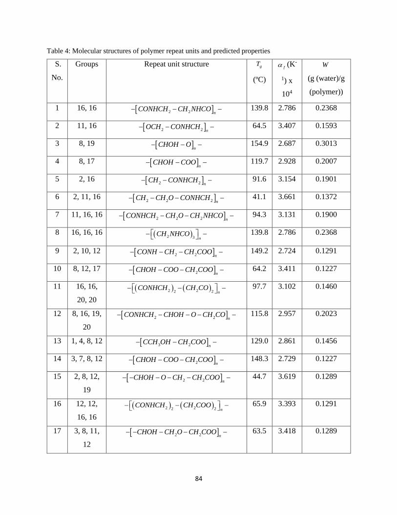
84

Table 4: Molecular structures of polymer repeat units and predicted properties

S.

No.

Groups Repeat unit structure gT

(ºC)

f (K-

1) x

104

W

(g (water)/g

(polymer))

1 16, 16 2 2 nCONHCH CH NHCO 139.8 2.786 0.2368

2 11, 16 2 2 nOCH CONHCH 64.5 3.407 0.1593

3 8, 19 n

CHOH O 154.9 2.687 0.3013

4 8, 17 n

CHOH COO 119.7 2.928 0.2007

5 2, 16 2 2 nCH CONHCH 91.6 3.154 0.1901

6 2, 11, 16 2 2 2 nCH CH O CONHCH 41.1 3.661 0.1372

7 11, 16, 16 2 2 2 nCONHCH CH O CH NHCO 94.3 3.131 0.1900

8 16, 16, 16 2 3 nCH NHCO 139.8 2.786 0.2368

9 2, 10, 12 2 2 nCONH CH CH COO 149.2 2.724 0.1291

10 8, 12, 17 2 nCHOH COO CH COO 64.2 3.411 0.1227

11 16, 16,

20, 20

2 22 2 nCONHCH CH CO 97.7 3.102 0.1460

12 8, 16, 19,

20

2 2 nCONHCH CHOH O CH CO 115.8 2.957 0.2023

13 1, 4, 8, 12 3 2 nCCH OH CH COO 129.0 2.861 0.1456

14 3, 7, 8, 12 2 nCHOH COO CH COO 148.3 2.729 0.1227

15 2, 8, 12,

19

2 2 nCHOH O CH CH COO 44.7 3.619 0.1289

16 12, 12,

16, 16

2 22 2 nCONHCH CH COO 65.9 3.393 0.1291

17 3, 8, 11,

12

2 2 nCHOH CH O CH COO 63.5 3.418 0.1289

85

18 8, 10, 12,

17

2 nCHOH COO CONH CH COO 157.0 2.674 0.1697

19 2, 8, 12,

14

2 2 nCCNOH CH CH COO 129.6 2.857 0.1261

20 11, 11,

16, 16, 20

2 2 22 2 nCONHCH CH O CH CO 59.8 3.455 0.1375

21 8, 13, 18,

20, 20

2 2 2 nNOH CH NH CH CO 42.7 3.643 0.2012

22 10, 10,

11, 12, 12

2 22 2 nCONH CH O CH COO 150.4 2.716 0.1296

23 16, 16,

16, 16, 20

2 24 nCONHCH CH CO 124.4 2.894 0.2073

24 16, 16,

20, 20, 20

2 22 3 nCONHCH CH CO 87.7 3.188 0.1372

25 12, 15,

16, 16, 20 2

2 22 n

CH COO CHCN

CONHCH CH CO

96.1 3.116 0.1245

26 4, 8, 8,

12, 20

2 22 nC OH CH COO CH CO 161.8 2.645 0.2077

27 8, 12, 12,

14, 16

2 22 nCCNOH CH COO CONHCH 111.8 2.988 0.1354

28 4, 5, 8, 8,

12

22 nC OH CH CH CH COO 160.0 2.656 0.2181

29 8, 8, 12,

19, 19

22 nCHOH O CH COO 92.4 3.147 0.1938

30 8, 8, 12,

14, 19

2 nCHOH O CCNOH CH COO 157.5 2.671 0.1879

31 1, 10, 12,

13, 18

3 2 2 nCH N CONH CH COO CH NH 79.2 3.265 0.1658

86

32 15, 15,

16, 16,

16, 16

2 4 2 nCONHCH CHCN 150.2 2.717 0.1841

33 16, 16,

18, 20,

20, 20

2 2 22 3 nCONHCH CH NH CH CO 172.0 2.584 0.1653

34 10, 16,

16, 20,

20, 20

2 22 3 nCONHCH CONH CH CO 141.5 2.774 0.1641

35 16, 16,

16, 16,

20, 20

2 24 2 nCONHCH CH CO 113.1 2.979 0.1858

36 16, 16,

16, 20,

20, 20

2 23 3 nCONHCH CH CO 97.7 3.102 0.1564

37 12, 12,

16, 16,

16, 16

2 24 2 nCONHCH CH COO 90.4 3.164 0.1648

38 16, 16,

16, 16,

16, 20

2 25 nCONHCH CH CO 127.0 2.875 0.2125

39 15, 16,

16, 16,

20, 20

2 23 2 nCHCN CONHCH CH CO 116.8 2.950 0.1552

The generated molecular structures are provided in the increasing order of the number of

groups in the repeat unit. This method does not take into account the order in which the groups are

attached to each other. As a result, with increasing number of groups in the repeat unit, there exist

several combinations of the groups to form the repeat unit structure. For example, if we consider,

repeat unit number 6, consisting of three different groups (group numbers 2, 11 and 16), there exist

3 different possible ways in which the repeat unit structure can be formed (not considering the

87

possibilities for isomers). The higher the number of groups in the repeat unit, the larger the number

of possible structures. This method does not distinguish between the various possibilities, as the

predicted property values are the same for all of them.

4.6.1 Ranking of Candidate Polymers

The candidate polymer structures generated can be further filtered based on their estimated

properties. The candidates can be ranked based on the desirability function as given by Eq. (11)

and Eq. (12). This method was developed by Harrington (Harrington 1965) and further modified

by Derringer and Suich (Derringer and Suich 1980). For each predicted property iY , a desirability

function (id ) is evaluated. The value of

id is always between 0 and 1. A id value of 1 implies that

a polymer with this property value is the most useful for the application, while a value of 0 makes

the polymer completely useless. Hence, the higher the value of id , the more useful the polymer

for the application. If we have multiple polymer properties with desired values, the corresponding

desirability can be evaluated using Eq. (17), where the composite desirability ( D ) is evaluated as

the geometric mean of the individual desirability’s.

1/

1 2 3( .... ) (17)k

kD d d d d

where, k is the number of properties considered. The value of D represents the optimality of the

polymer considered and has is value between 0 and 1 like the individual desirability’s (Derringer

and Markham 1985).

We plotted desirability curves based on some of the properties considered such as gT and

W . In case of gT , as shown in Fig. 1, the most desirable value is 107 ºC, which is midway between

37 ºC and 177 ºC. The polymer must possess high glass transition so that the formulation can be

transferred and stored for months. Also the polymer must not itself have a tendency to crystallize

(Hancock and Parks 2000, Konno and Taylor 2006). It is preferable that all crystallinity of the drug

substance be suppressed by the polymer carrier since small pockets of crystallinity can act as seeds,

resulting in additional crystal growth and ultimately reduced shelf-life of the drug formulation

(Florence et al. 2011). Normally during summers, the temperature in certain regions reaches close

to 50 ºC. So the gT value must be 40-50 ºC higher than the storage temperature. Therefore a

88

temperature around 100 ºC is a reasonable value for desirable gT . The higher the value of

gT , the

more difficult it is for the polymer to transform into rubbery state once it is inside the body. So a

gT value below 107 ºC is much more favorable compared to a value above 107 ºC. Hence in Fig.

3, the desirability function is adjusted in such a way that, the curve falls more slowly below 107

ºC and much faster above 107 ºC. This is done by adjusting the values of the variables s and t in

Eq. (11) and Eq. (12). For Fig. 2, the value of s is 0.3 and the value of t is 3. Table 5 gives a list

of the top six, most favorable structures based on desirability ranking using gT .

Figure 2: Desirability curve using glass transition temperature (gT )

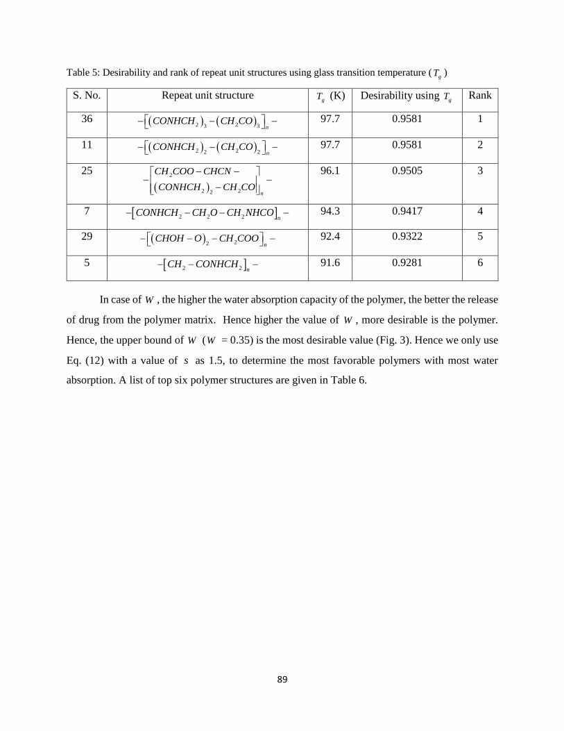
89

Table 5: Desirability and rank of repeat unit structures using glass transition temperature (gT )

S. No. Repeat unit structure gT (K) Desirability using

gT Rank

36 2 23 3 nCONHCH CH CO 97.7 0.9581 1

11 2 22 2 nCONHCH CH CO 97.7 0.9581 2

25

2

2 22 n

CH COO CHCN

CONHCH CH CO

96.1 0.9505 3

7 2 2 2 nCONHCH CH O CH NHCO 94.3 0.9417 4

29 22 nCHOH O CH COO 92.4 0.9322 5

5 2 2 nCH CONHCH 91.6 0.9281 6

In case of W , the higher the water absorption capacity of the polymer, the better the release

of drug from the polymer matrix. Hence higher the value of W , more desirable is the polymer.

Hence, the upper bound of W (W = 0.35) is the most desirable value (Fig. 3). Hence we only use

Eq. (12) with a value of s as 1.5, to determine the most favorable polymers with most water

absorption. A list of top six polymer structures are given in Table 6.

90

Figure 3: Desirability curve using water absorption (W )

Table 6: Desirability and rank of repeat unit structures using water absorption (W )

S. No. Repeat unit structure W

(g (water)/

g

(polymer))

Desirability using W Rank

3 n

CHOH O 0.3013 0.7225 1

8 2 3 nCH NHCO 0.2368 0.4048 2

1 2 2 nCONHCH CH NHCO 0.2368 0.4048 3

28 22 nC OH CH CH CH COO 0.2181 0.3247 4

38 2 25 nCONHCH CH CO 0.2125 0.3019 5

26 2 22 nC OH CH COO CH CO 0.2077 0.2827 6

91

4.6.2 Solubility Parameter Analysis

The solubility of a polymer is largely dependent on its chemical structure. The miscibility of two

materials is more favored when they are structurally similar. The comparison of solubility

parameters between two materials determines their extent of miscibility. The solubility parameter

( ) is a numerical value, which determines the relative miscibility between two materials and is

defined as the square root of cohesive energy density (cohesive energy per unit volume). The

cohesive energy of a solid is the energy required to break the atoms of the solid into isolated atomic

species. The solubility parameter value can be estimated using a group contribution method

proposed by Hansen (Hansen 1969), and is given by Eq. (18).

2 2 2

2

(18)

where,

d p h

pidi hi

d p h

i i i

FF F

V V V

where, diF ,

piF and hiF are the additive atomic and group contributions to cohesive energy from

dispersion forces, polarity and hydrogen bonds of a structural group i , and iV is the group

contribution for molar volume, respectively. Table 7 gives a list of some of the well-known

pharmaceutical drugs and their corresponding solubility parameters (Gupta 2011). It also gives a

list of the solubility parameters of the generated polymer structures evaluated using the Hansen

method. This table contains only the list of polymers which have a comparable solubility parameter

value to that of the drugs. Here the polymers are represented using their serial numbers, which are

used in Table 4, and both the drugs and polymers are arranged in the increasing order of their

value. For example, Ibuprofen has a solubility parameter closest to the polymer with S. No. 5,

indicating that it is most miscible with that polymer.

92

Table 7: Comparison of solubility parameters of pharmaceutical drugs and generated polymers

Drug Solubility

Parameter ( ) (MPa0.5)

Polymer

S. No.

Solubility

Parameter ( ) (MPa0.5)

Ibuprofen 19.2 5 22.7

Napthalene 20.1 33 24.1

Pimozide 21.1 35 24.3

Haloperidol 22.1 36 24.3

Naproxen 22.7 38 24.3

Phenylbutazone 22.7 23 24.4

Diazepam 22.9 24 24.5

Caffeine 23.2 11 24.8

Prazepam 23.2 8 24.8

Niflumic acid 23.6 39 25.2

Trimethoprim 23.7 1 25.4

Rofecoxib 24.8 34 25.7

Diclofenac 25.1 20 25.9

Temazepam 25.4 32 26.2

Paracetamol 25.5 37 27.4

p-Aminobenzoic acid 25.7 6 27.4

Lorazepam 25.9 7 27.5

Oxazepam 27.3 25 28.3

Theophylline 27.4 16 31.3

p-Hydroxybenzoic acid 27.6 31 32.3

Piroxicam 28.6 21 32.7

Citric acid 29.3 2 32.7

Meloxicam 29.3 12 36.1

Sucrose 30 27 37.4

Mannitol 32 22 37.8

Lactose 40.5 9 40.4

93

The compounds that are thermodynamically miscible will have similar values of . There

is an established classification system in the literature for predicting the miscibility of drug and

polymers, based on the solubility parameter differences ( ). According to Greenhalgh et. al.

(Greenhalgh et al. 1999), compounds with < 7.0 MPa0.5 are likely to be miscible, while for

> 10.0 MPa0.5, the compounds are completely immiscible. According to Foster et. al. (Forster et

al. 2001), compounds that are miscible have < 2.0 MPa0.5. In Table 7 we observe that, there are

several drugs and polymers with comparable solubility parameters or with < 2.0 MPa0.5. For

example if we take a very well known drug, Paracetamol with a value of 25.5. The polymers,

which have an almost equal value of, are with serial numbers 1, 34, 39, 20 with increasing value

of . Similarly, Paracetamol is almost immiscible with polymer of serial numbers 2, 12, 27, 22,

9 with increasing value of . Therefore, the greater the miscibility between the polymer and

drug, the more likely the polymer would be able to suppress the crystallinity of the drug. This is

the basis for formation of amorphous solid dispersions (ASD’s) for drug delivery. Through this

method of comparison, one can identify the most compatible polymer and drug combinations

having the best miscibility. This is an effective strategy to filter the polymer candidates generated

based on their compatibility with the drug candidates.

The solubility parameters shown in Table 7 dictate the relative hydrophobicity of the novel

polymers generated. The solubility parameter provides a numerical estimate of the intermolecular

forces within a material and can be a good indication of solubility (Ilevbare et al. 2012). The higher

the solubility parameter, more hydrophilic it is.

4.7 Sensitivity and Uncertainty Analysis

All the group contribution parameters used in the CAMD method have an error margin. This means

that it is quite possible that some of the feasible molecules will be eliminated due to errors in the

property predictions. In order to ensure the accuracy of the method, we performed sensitivity and

uncertainty analysis.

We performed parameter sensitivity analysis to analyze the relative sensitivity of model

output with respect to the changing parameter values and identifying the most important ones. The

parameters in our case are the group contribution of the relevant groups specific to each of the

94

properties. We performed uncertainty analysis to determine the accuracy of the group contribution

method based on the group contribution parameter values and their standard deviations.

We chose a sample molecule generated through the CAMD method, which in this case is

molecule with serial number 25 and ranked 3rd in Table 5, and perform sensitivity and uncertainty

analysis on this molecule and discuss the results obtained. The sensitivity analysis is done by

sequentially varying the model parameters by fixing all the other parameters to their nominal

values to determine the model output. Normalized sensitivity coefficient ( NSC ) values are

evaluated from the values obtained using Eq. (19) (Chung 2009). NSC values indicate the

importance of a parameter on the model output.

0 0

0 0

( ) /(19)

( ) /NSC

P P P

where, is the nominal value of the model output at P0 the nominal value of the parameter;

similarly is the model output at P. The model output is evaluated using Eq. (10).

The sample molecule with serial number 25 is made up of 4 different groups, namely,

2CH COO , CHCN , 2CONHCH and

2CH CO . The contribution parameter and standard deviation

values for each of these groups can be obtained from Table 8.

Table 8: Group contribution parameters and standard deviations for molar glass transition temperature

Group Molar glass transition

function

(giY ) (gm.K/mol)

Standard deviation (%)

2CH COO 15447.25 18.91

CHCN 17695.43 34.17

2CONHCH 23529.58 18.94

2CH CO 13169.56 28.59

0

95

Figure 4: Sensitivity analysis of group contribution parameters

The contribution parameters for each group mentioned in Table 8 are varied according to

their standard deviations, keeping the values of other groups a constant and observed the effect on

the estimated gT value. The corresponding NSC values are evaluated and plotted in Fig. 4. We

observed that, the NSC values are maximum for the 2CONHCH group, followed by CHCN ,

followed by 2CH COO , and finally

2CH CO group being the least sensitive. This indicated the

sensitivity of groups from highest to lowest in the same order. We observe that the sensitivity

increases with increase in the contribution parameter value. Since the glass transition temperature

is estimated as given in Eq. (6), with increase or decrease in the contribution parameter value of a

certain group, there is a corresponding increase or decrease in the NSC value.

We have done uncertainty analysis to see the variability of the group contributions

parameters and their effect on the model output. This analysis determined if the parameter values

96

when taken to the extremes of their standard deviations, satisfy the model constraints. We varied

the group parameter values according to the standard deviation values given in Table 8. A plot

comparing the contribution parameter of molar glass transition temperature with the estimated

glass transition temperature value is given in Fig. 5.

Figure 5: Uncertainty analysis of group contribution parameters

We observed that, there is a proportional change in the estimated property value, which in

this case is the gT value, with change in the contribution parameter value. The lines corresponding

to the groups 2CH CO ,

2CH COO , and CHCN are parallel because they have an equal slope of 1

mol/gm as they appear once in the repeat unit. While the line corresponding to 2CONHCH has a

slope of 2 mol/gm because it appears twice in the repeat unit. Fortunately in our case, the estimated

gT value is within the acceptable bounds of 37 ºC to 177 º as described in Table 3, even when the

contribution parameter values are varied to the extremes of their standard deviation values.

97

However, if the acceptable bounds of gT are changed to 77 ºC K to 107 ºC as shown in Fig. 4, we

observe that some of the estimated gT values fall outside the bounds with change in the

contribution parameter values. A minor part of the curves for the groups 2CH CO and

2CH COO

fall outside the bounds, while a significant portion of the curves for the groups CHCN and

2CONHCH fall outside the bounds. This indicates that there is a high possibility of the molecule

becoming a failure due to the standard deviation values of the contribution parameters. One

solution to this issue is to improve the accuracy of the group contribution parameters by using

greater sample size to estimate the parameter value. We can assign confidence intervals to the

contribution parameter values by further analyzing the plot as shown in Fig. 4 for the 2CONHCH

group.

4.8 Conclusions

A CAMD framework is used to generate molecular structures of polymers with desired properties.

We have successfully generated molecular structures of repeat units of polymers which have the

potential to be used as efficient carrier materials for drug delivery. The properties used in the

problem formulation, namely, glass transition temperature (gT ), expansion coefficient (

f ) and

water absorption (W ) were effective in reducing the number of possible candidates to a few. As

the total number of groups in the repeat unit increased, the number of possible ways in which the

repeat unit could be formed increased accordingly. This method does not provide us with a strategy

on the how to form the repeat unit, once we have the groups. Hence, there is no distinguishing

between the several possible repeat units, as the properties estimated for each of them are same.

The formulation does not take into account the constraints based on bond angles. A group

contribution method which could consider bond angles and be able to distinguish between different

structures in a systematic manner is desired.

The generated polymer structures are ranked using desirability curves. The desirability

curves are developed based on a desired property value. We were able to successfully rank the

candidates based on the desirability developed using glass transition temperature (gT ) and water

absorption (W ). The desirability curve is an effective tool to rank the polymer candidates

98

according to their usability. The higher their desirability value, the more useful the polymer is for

the intended application.

A solubility parameter analysis was done to further analyze and filter the polymer

candidates. It served as an effective strategy to filter the polymer candidates based on their

compatibility with the pharmaceutical drugs. Two compounds with the most similar solubility

parameter value are the most miscible. This principle has been effectively used to develop the

strategy.

The generated molecular structures using this methodology need further investigation for

them to be used for drug delivery applications. An expert opinion from a polymer chemist about

the validity of the generated structures is very essential. An opinion about the possibility of

synthesizing the new polymers, the practicality and economics involved, will greatly help in

progress of this work.

Sensitivity analysis was done for one of the candidate polymers generated and evaluated

the NSC values. A change in the contribution parameter value corresponds to a change in the NSC

value. The sensitivity of a group contribution parameter increases with increase in the contribution

value. Uncertainty analysis revealed that contribution parameter values when changed to the

extremes of their standard deviation can make the estimated property value fall out of the

acceptable bounds. This can potentially lead to candidate failures. There is need for greater

accuracy in the estimated group contribution parameter values to avoid greater uncertainties in the

candidate selection process.

The MINLP optimization used to solve the CAMD problem give a local optimum solution.

Thus there are multiple solutions based on the starting points. This is one of the major reasons for

high computational times, because of the existence of multiple feasible solutions. An excellent

way to avoid repeating solutions is to introduce constraints based on heuristics. For example, a

constraint can be formed to update the bounds after each iteration to change the feasibility region

and avoid repeatability. This would definitely help in eliminating the problem but would increase

the complexity of the formulation.

99

The developed CAMD methodology helps in selecting the most favorable candidates

having the desired properties. It greatly helps in the product development process by reducing the

number of experimental trials, hence reducing the time and effort involved. It helps in identifying

potential failures in the early development process, thereby avoiding late stage failures. We expect

our work to greatly aid in the overall product development process.

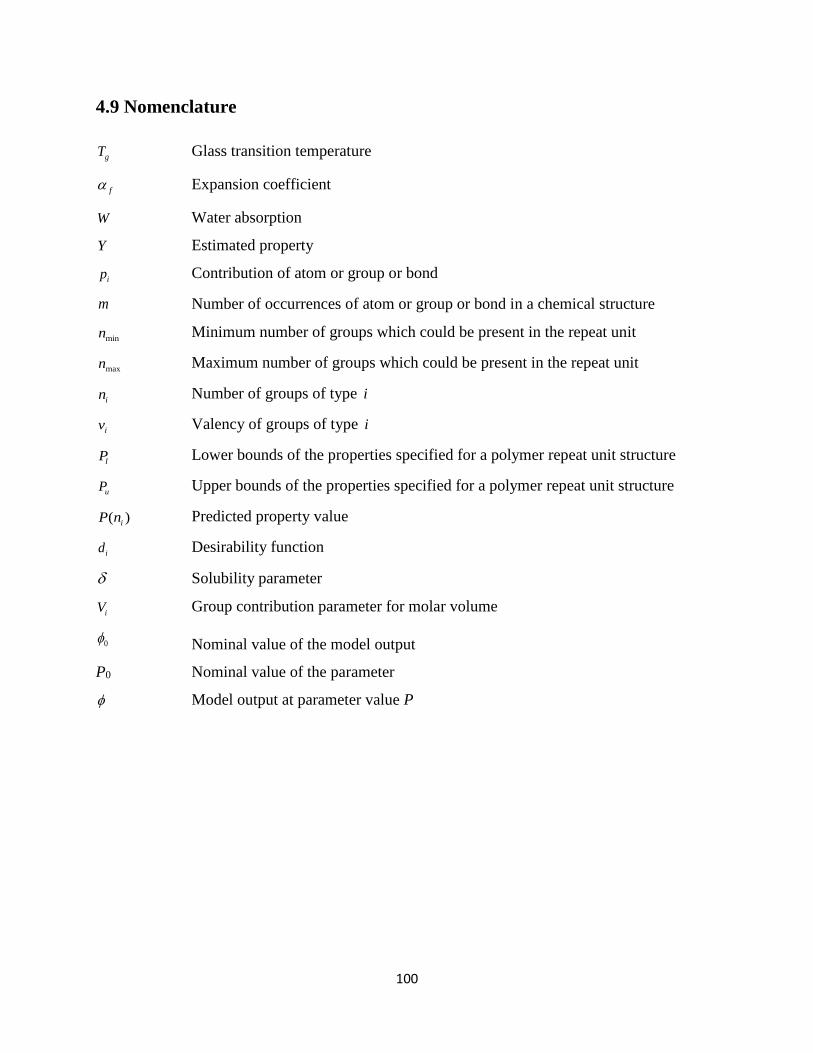
100

4.9 Nomenclature

gT Glass transition temperature

f Expansion coefficient

W Water absorption

Y Estimated property

ip Contribution of atom or group or bond

m Number of occurrences of atom or group or bond in a chemical structure

minn Minimum number of groups which could be present in the repeat unit

maxn Maximum number of groups which could be present in the repeat unit

in Number of groups of type i

iv Valency of groups of type i

lP Lower bounds of the properties specified for a polymer repeat unit structure

uP Upper bounds of the properties specified for a polymer repeat unit structure

( )iP n Predicted property value

id Desirability function

Solubility parameter

iV Group contribution parameter for molar volume

Nominal value of the model output

P0 Nominal value of the parameter

Model output at parameter value P

0

101

4.10 References

Andrianov, A. K. and L. G. Payne (1998). "Protein release from polyphosphazene matrices."


Attawia, M. A., M. D. Borden, K. M. Herbert, D. S. Katti, F. Asrari, K. E. Uhrich and C. T.

Laurencin (2001). "Regional drug delivery with radiation for the treatment of Ewing’s sarcoma:

In vitro development of a taxol release system." Journal of Controlled Release 71(2): 193-202.

Bae YH, K. S. (1998). Drug delivery. Frontiers in tissue engineering. M. A. Patrick CW, Mcintire

LV Oxford: 261.

Barbucci, R. (2002). Integrated Biomaterials Science. New York, Kluwer Plenum

Bezemer, J. M., D. W. Grijpma, P. J. Dijkstra, C. A. van Blitterswijk and J. Feijen (2000). "Control

of protein delivery from amphiphilic poly(ether ester) multiblock copolymers by varying their

water content using emulsification techniques." Journal of Controlled Release 66(2–3): 307-320.

Bicerano, J. (2002). Prediction of Polymer Properties. New York, Marcel Dekker. Inc.

Blanco, M. D., M. V. Bernardo, R. L. Sastre, R. Olmo, E. Muñiz and J. M. Teijón (2003).

"Preparation of bupivacaine-loaded poly(ε-caprolactone) microspheres by spray drying: drug

release studies and biocompatibility." European Journal of Pharmaceutics and Biopharmaceutics

55(2): 229-236.

Brüggemann, I. T. a. O. (2013). "Polyphosphazenes: Multifunctional, Biodegradable Vehicles for

Drug and Gene Delivery." Polymers 2013 5(161-187).

Camarda, K. V. and C. D. Maranas (1999). "Optimization in Polymer Design Using Connectivity

Indices." Industrial & Engineering Chemistry Research 38(5): 1884-1892.

Chiu Li, L., J. Deng and D. Stephens (2002). "Polyanhydride implant for antibiotic delivery—

from the bench to the clinic." Advanced Drug Delivery Reviews 54(7): 963-986.

Choi, H. J., Yang, R., Kunioka, M. (1995). "Synthesis and characterization of pH-sensitive and

biodegradable hydrogels prepared by γ irradiation using microbial poly(γ-glutamic acid) and

poly(ϵ-lysine)." Journal of Applied Polymer Science 58(4): 807-814.

102

Chung, S.-W., Miles, Fayth L., Sikes, Robert A., Cooper, Carlton R., Farach-Carson, Mary C.,

Ogunnaike, Babatunde A. (2009). "Quantitative Modeling and Analysis of the Transforming

Growth Factor ² Signaling Pathway." Biophysical journal 96(5): 1733-1750.

Churi, N. and L. E. K. Achenie (1996). "Novel Mathematical Programming Model for Computer

Aided Molecular Design." Industrial & Engineering Chemistry Research 35(10): 3788-3794.

Cynthia D’Avila Carvalho Erbetta, R. J. A., Jarbas Magalhães Resende, Roberto Fernando de

Souza Freitas, Ricardo Geraldo de Sousa (2012). "Synthesis and Characterization of Poly(D,L-

Lactide-co-Glycolide) Copolymer." Journal of Biomaterials and Nanobiotechnology 3: 208-225.

Derringer, G. and R. Suich (1980). "{Simultaneous optimization of several response variables}."

Journal of quality technology 12(4): 214-219.

Derringer, G. C. and R. L. Markham (1985). "A computer-based methodology for matching

polymer structures with required properties." Journal of Applied Polymer Science 30(12): 4609-

4617.

Dossi, M., G. Storti and D. Moscatelli (2010). "Synthesis of Poly(Alkyl Cyanoacrylates) as

Biodegradable Polymers for Drug Delivery Applications." Macromolecular Symposia 289(1):

124-128.

Duvedi, A. P. and L. E. K. Achenie (1996). "Designing environmentally safe refrigerants using

mathematical programming." Chemical Engineering Science 51(15): 3727-3739.

Ertel, S. I. and J. Kohn (1994). "Evaluation of a series of tyrosine-derived polycarbonates as

degradable biomaterials." Journal of Biomedical Materials Research 28(8): 919-930.

Esposito, E. X., Hopfinger, A.J., Madura, J.D. (2004). Methods for Applying the Quantitative

Structure-Activity Relationship Paradigm. 275: 131-213.

Florence, A. T., D. Attwood and D. Attwood (2011). Physicochemical principles of pharmacy,

Pharmaceutical Press.

Floudas, C. A. (1995). Nonlinear and mixed-integer optimization: fundamentals and applications,

Oxford University Press.

103

Forster, A., J. Hempenstall, I. Tucker and T. Rades (2001). "Selection of excipients for melt

extrusion with two poorly water-soluble drugs by solubility parameter calculation and thermal

analysis." International Journal of Pharmaceutics 226(1–2): 147-161.

Gani, R. and L. Constantinou (1996). "Molecular Structure Based Estimation of Properties for

Process Design." Fluid Phase Equilibria 116(1): 75-86.

Gasteiger, J. and T. Engel (2003). Chemoinformatics, Wiley-VCH.

Gaucher, G., P. Satturwar, M.-C. Jones, A. Furtos and J.-C. Leroux (2010). "Polymeric micelles

for oral drug delivery." European Journal of Pharmaceutics and Biopharmaceutics 76(2): 147-158.

Greenhalgh, D. J., A. C. Williams, P. Timmins and P. York (1999). "Solubility parameters as

predictors of miscibility in solid dispersions." Journal of Pharmaceutical Sciences 88(11): 1182-

1190.

Gupta, J., Nunes, C., Vyas, S., Jonnalagadda, S. (2011). "Prediction of Solubility Parameters and

Miscibility of Pharmaceutical Compounds by Molecular Dynamics Simulations." The Journal of

Physical Chemistry B 115(9): 2014-2023.

Hamdy Abdelkader, O. Y. A., and Hesham Salem (2008). "Formulation of Controlled-Release

Baclofen Matrix Tablets II: Influence of Some Hydrophobic Excipients on the Release Rate and

In Vitro Evaluation." AAPS PharmaSciTech 9(2): 675-683.

Hancock, B. C. and M. Parks (2000). "What is the true solubility advantage for amorphous

pharmaceuticals?" Pharmaceutical research 17(4): 397-404.

Hansen, C. M. (1969). "The Universality of the Solubility Parameter." Product R&D 8(1): 2-11.

Harmia, T., J. Kreuter, P. Speiser, T. Boye, R. Gurny and A. Kubi (1986). "Enhancement of the

myotic response of rabbits with pilocarpine-loaded polybutylcyanoacrylate nanoparticles."

International Journal of Pharmaceutics 33(1–3): 187-193.

Harper, P. M., Gani, Rafiqul, Kolar, Petr, Ishikawa, Takeshi (1999). "Computer-aided molecular

design with combined molecular modeling and group contribution." Fluid Phase Equilibria 158–

160(0): 337-347.

104

Harrington, E. C. (1965). "The desirability function." Industrial Quality Control(21): 494-498.

Heller, J., J. Barr, S. Y. Ng, H. R. Shen, K. Schwach-Abdellaoui, R. Gurny, N. Vivien-Castioni,

P. J. Loup, P. Baehni and A. Mombelli (2002). "Development and applications of injectable

poly(ortho esters) for pain control and periodontal treatment." Biomaterials 23(22): 4397-4404.

Ilevbare, G. A., H. Liu, K. J. Edgar and L. S. Taylor (2012). "Understanding Polymer Properties

Important f

Crystal Growth of Ritonavir." Crystal Growth & Design 12(6): 3133-3143.

Illum, L., A. N. Fisher, I. Jabbal-Gill and S. S. Davis (2001). "Bioadhesive starch microspheres

and absorption enhancing agents act synergistically to enhance the nasal absorption of

polypeptides." International Journal of Pharmaceutics 222(1): 109-119.

Izawa, H., Kawakami, K., Sumita, M., Tateyama, Y., Hill, J.P., Ariga, K. (2013). "[small beta]-

Cyclodextrin-crosslinked alginate gel for patient-controlled drug delivery systems: regulation of

host-guest interactions with mechanical stimuli." Journal of Materials Chemistry B 1(16): 2155-

2161.

Jadhav, N. R., Gaikwad, V.L., Nair, K.J., Kadam, H.M. (2009). "Glass transition temperature:

Basics and application in pharmaceutical sector." Asian J Pharm 3: 82-89.

Jain, J. P., D. Chitkara and N. Kumar (2008). "Polyanhydrides as localized drug delivery carrier:

an update." Expert Opinion on Drug Delivery 5(8): 889-907.

Jain, J. P., W. Yenet Ayen, A. J. Domb and N. Kumar (2011). Biodegradable Polymers in Drug

Delivery. Biodegradable Polymers in Clinical Use and Clinical Development, John Wiley & Sons,

Inc.: 1-58.

Karunanithi, A. T., Achenie, Luke E. K., Gani, Rafiqul (2005). "A New Decomposition-Based

Computer-Aided Molecular/Mixture Design Methodology for the Design of Optimal Solvents and

Solvent Mixtures." Industrial & Engineering Chemistry Research 44(13): 4785-4797.

Karunanithi, A. T., Achenie, Luke E. K., Gani, Rafiqul (2006). "A computer-aided molecular

design framework for crystallization solvent design." Chemical Engineering Science 61(4): 1247-

1260.

105

Kassab, A. C., K. Xu, E. B. Denkbas, Y. Dou, S. Zhao and E. Piskin (1997). "Rifampicin carrying

polyhydroxybutyrate microspheres as a potential chemoembolization agent." Journal of

Biomaterials Science, Polymer Edition 8(12): 947-961.

Kier, L. B. and H. L. Hall (1986). Molecular Connectivity in Structure Acivity Analysis. New

York, John Wiley & Sons.

Konno, H. and L. S. Taylor (2006). "Influence of different polymers on the crystallization tendency

of molecularly dispersed amorphous felodipine." Journal of pharmaceutical sciences 95(12): 2692-

2705.

Lakshmi, S., D. S. Katti and C. T. Laurencin (2003). "Biodegradable polyphosphazenes for drug

delivery applications." Advanced Drug Delivery Reviews 55(4): 467-482.

Lewis, D. H. (1990). Controlled release of bioactive agents from lactide/glycolide polymers. New

York, Marcel Dekker.

Li, C., Yu, D.F., Newman, R.A., Cabral, F., Stephens, L.C., Hunter, N., Milas, L., Wallace, S.

(1998). "Complete Regression of Well-established Tumors Using a Novel Water-soluble Poly(l-

Glutamic Acid)-Paclitaxel Conjugate." Cancer Research 58(11): 2404-2409.

Magdalena M. Stevanović, B. J., and Dragan P. Uskoković (2007). "Preparation and

Characterization of Poly(D,L-Lactide-co-Glycolide) Nanoparticles Containing Ascorbic Acid."

Journal of Biomaterials and Biotechnology 2007:84965.

Maranas, C. D. (1996). "Optimal Computer-Aided Molecular Design: A Polymer Design Case

Study." Industrial & Engineering Chemistry Research 35(10): 3403-3414.

Marrero, J. and R. Gani (2001). "Group Contribution Based Estimation of Pure Component

Properties." Fluid Phase Equilibria 183: 183-184.

Mathiowitz, E. (1999). Encyclopedia of controlled drug delivery. New York, Wiley.

Moore, E. L. and T. J. Peters (2005). "Computational topology for geometric design and molecular

design." Mathematics for Industry: Challenges and Frontiers. SIAM: 125-137.

106

Mumper, R. J., Hoffman, A.S., Puolakkainen, P.A., Bouchard, L.S., Gombotz, W.Z. (1994).

"Calcium-Alginate Beads for the Oral Delivery of Transforming Growth Factor-B1 (TGF-B1):

Stabilization of TGF-B1 by the Addition of Polyacrylic Acid Within Acid-Treated Beads." J.

Controlled Rel. 30: 241-251.

Nair, L. and C. Laurencin (2006). Polymers as Biomaterials for Tissue Engineering and Controlled

Drug Delivery. Tissue Engineering I. K. Lee and D. Kaplan, Springer Berlin Heidelberg. 102: 47-

90.

Nicolas, J. and P. Couvreur (2009). "Synthesis of poly(alkyl cyanoacrylate)-based colloidal

nanomedicines." Wiley Interdisciplinary Reviews: Nanomedicine and Nanobiotechnology 1(1):

111-127.

Ostrovsky, G. M., L. E. Achenie and M. Sinha (2002). "On the solution of mixed-integer nonlinear

programming models for computer aided molecular design." Comput Chem 26(6): 645-660.

Phaechamud, T. (2008). "Variables Influencing Drug Release from Layered Matrix System

Comprising Hydroxypropyl Methylcellulose." AAPS PharmaSciTech 9(2): 668-674.

Randić, M. (2001). "The connectivity index 25 years after." Journal of Molecular Graphics and

Modelling 20(1): 19-35.

Robert, H., Marchessault1, François Ravenelle, Xiao Xia Zhu (2006). Polysaccharides for Drug

Delivery and Pharmaceutical Applications. F. R. Robert H. Marchessault1, Xiao Xia Zhu,

American Chemical Society.

Rosen, H. B., J. Chang, G. E. Wnek, R. J. Linhardt and R. Langer (1983). "Bioerodible

polyanhydrides for controlled drug delivery." Biomaterials 4(2): 131-133.

Shrivastav, A., Kim, H., Kim, Y. (2013). "Advances in the Applications of Polyhydroxyalkanoate

Nanoparticles for Novel Drug Delivery System." BioMed Research International 2013: 12.

Sola, D., A. Ferri, M. Banchero, L. Manna and S. Sicardi (2008). "QSPR prediction of N-boiling

point and critical properties of organic compounds and comparison with a group-contribution

method." Fluid Phase Equilibria 263(1): 33-42.

107

Swarbrick, J., Boyan, H.C. (1991). Gels and jellies In:Encyclopedia of pharmaceutical technology

Newyork, Marcel Dekker.

Timmerman, H., Mannhold, R., Krogsgaard-Larsen, P., Waterbeemd, H. (2008). Chemometric

methods in molecular design, Wiley. com.

Tønnesen, H. H., Karlsen, J. (2002). "Alginate in Drug Delivery Systems." Drug Development and

Industrial Pharmacy 28(6): 621-630.

Ueda, H., Tabata, Y. (2003). "Polyhydroxyalkanonate derivatives in current clinical applications

and trials." Advanced Drug Delivery Reviews 55(4): 501-518.

Van Krevelen, D. W. (1990). Properties of Polymers. Amsterdam, Elsevier.

Venkatasubramanian, V., Chan, K., Caruthers, J.M. (1994). "Computer-aided molecular design

using genetic algorithms." Computers & Chemical Engineering 18(9): 833-844.

Venkatasubramanian, V., Chan, K., Caruthers, J.M. (1995). Genetic Algorithmic Approach for

Computer-Aided Molecular Design. Computer-Aided Molecular Design, American Chemical

Society. 589: 396-414.

Vert, M., G. Schwach, R. Engel and J. Coudane (1998). "Something new in the field of PLA/GA

bioresorbable polymers?" Journal of Controlled Release 53(1–3): 85-92.

Wolber, G., Seidel, T., Bendix, F., Langer, T. (2008). "Molecule-pharmacophore superpositioning

and pattern matching in computational drug design." Drug discovery today 13(1): 23-29.

Yuan, H., K. Luo, Y. Lai, Y. Pu, B. He, G. Wang, Y. Wu and Z. Gu (2010). "A Novel Poly(l-

glutamic acid) Dendrimer Based Drug Delivery System with Both pH-Sensitive and Targeting

Functions." Molecular Pharmaceutics 7(4): 953-962.

Zhao, Z., J. Wang, H.-Q. Mao and K. W. Leong (2003). "Polyphosphoesters in drug and gene

delivery." Advanced Drug Delivery Reviews 55(4): 483-499.

108

4.11 Appendix A

A list of polymers which are currently being used as carriers for pharmaceutical drugs and the

corresponding groups extracted from the individual molecular structures of each polymer.

Table A1: List of polymers used in drug delivery as carrier materials

Polymer Repeat unit structure Corresponding groups

Polycaprolactone

(PCL)

2 2 2, ,CH CO CH O CH

Poly (dimethyl

siloxane) (PDMS)

3 ,CH SiO

Polyurethanes

,CONH COO

Poly (vinyl chloride)

(PVC)

2,CHCl CH

Poly (hexamethylene

adipamide) (Nylon

6,6)

2 2, ,CH NH CONH CH CO

Poly (methyl

methacrylate)

(PMMA)

3 2, , ,CH CH C COO

Poly (lactide-co-

glycolide) (PLGA)

3 2, ,CH CHO CH CO

Polydioxanone (PDO)

2 2,CH COO CH O

Poly (sebacic acid)

2 2, ,CH COO COO CH

Poly (ortho esters)

2 2, ,CH O C CH

109

Poly anhydrides

3 , , ,CH N CH CHCOO

Poly (alkyl

cyanoacrylate)

2 , ,CH CCN COO

Poly (amino acids)

2 , ,CH CONH COO CHCOO

Cellulose

2 , ,CH CH OH

Proteins

,CONH CH

Polyhydroxyalkanoate

s

2,CHO CH CO

Poly (propylene

fumarate)

, ,OH CH CH COO

110

CHAPTER 5

Customization of Oral Drug Dosage Form – Innovation in Tablet

Design

Abstract

Novel tablet designs (oral drug dosage forms) are proposed which could lead to desired drug

release profiles. The targeted drug release profiles include constant or zero-order release, Gaussian

release and pulsatile release. The proposed design are supported through mathematical modeling

and simulations along with logical and sound explanations. A drug release model was used to

simulate tablet designs; it successfully simulated a constant release and a pulsatile release. The

duration of the drug release can be controlled by varying the dissolution rate of the polymer matrix

in case of constant release. The delay between consecutive pulse releases can be controlled by

varying the dissolution rate of the pH sensitive polymer barrier as well as its thickness.

Keywords: tablet customization, oral drug tablet, polymer matrix, drug release profile, polymer

barrier, rigid polymer


In this chapter, we propose some innovative tablet designs (oral dosage form), which could lead

to a desired drug release profile. A desired drug release profile is inspired by a desired plasma

concentration profile of drug in the blood of the human body. A desired plasma concentration

profile is a representation of the desired therapeutic for the patient (Fig. 1).

111

Figure 1: Interdependence of plasma profile, drug release profile and tablet design

We proposed tablet designs for specific desired release profiles such as a constant release

(zero order) release, a Gaussian release and a pulsatile release. Different release profiles specified

are desired for different kinds of diseases. This work is expected to have a significant impact on

the approach to tablet design in the pharmaceutical industry. The customization of oral dosage

form is inspired by the idea of providing desired therapeutic effect to each individual patient based

on his/her physiological and genetic makeup. It is an important step towards the development of

personalized medicine.


The plasma concentration profile or the final concentration of blood in the plasma is dependent on

the patient’s metabolic rate. Once we know the amount of drug in the plasma and the

bioavailability of the drug, one can estimate the amount of active pharmaceutical ingredient (API)

that has to go into manufacturing the dosage form for each of the individual patients. In order to

obtain the desired therapeutic effect specific to each patient, the tablets are cast into several shapes

and sizes. A final customized tablet will ensure that the specific targeted patient will receive the

most effective dosage of the API at a rate unique to that individual.

Desired Therapeutic Effect

Plasma Concentration Profile

Desired Release Profile

Drug Release Profile

Tablet Design (Dosage Form)

112

Most of the pharmaceutical drugs are manufactured in standard forms with limited range

of dosage strengths. Thus a patient is forced to depend on a limited number of ways in which the

dose could be administered for maximum effectiveness. This may sometimes lead to toxicity issues

due to overdose of the drug, while it may lead to ineffectiveness of the drug in some patients due

to insufficient drug dose. This generally varies from patient to patient based on their individual

metabolic rates.

Drug delivery devices like reservoir or matrices are important means of delivering the drug

at a given rate and duration. The delivery devices are chosen based on the type of drug and delivery

kinetics. Matrices are considered more reliable in terms of delivery, less expensive, easier to

formulate and less malfunctioning problem. There are several types of matrices such as inert,

erodible and swellable. However, we restrict our discussion to swellable matrix given our area of

interest.

5.2.1 Polymer Matrix Tablet

In a polymer matrix tablet, the drug is embedded inside a dry polymer. When the polymer comes

in contact with the water, it swells and allows the drug to move freely through the swollen polymer.

The transport of water through the swollen polymer and the rate of swelling of the polymer are

two important factors governing the release of drug from the tablet. Some examples of polymers

that are being used in synthesizing matrix tablets are: methylcellulose, hydroxypropyl

methylcellulose, polyvinylpirrolyone, or sodium alginate (Wesselingh and Frijlink 2008).

The swelling of a matrix in an aqueous medium of a given drug and a chosen polymer

determines the drug release rate from a system which is continuously transforming and then

dissolves completely. Apart from the interactions between water, polymer and drug which are the

primary factors for controlling the drug release rate, other variables which affect the drug release

are drug to polymer ratio, drug solubility, polymer grade (molecular weight and viscosity), filter

solubility, drug and polymer particle size and compaction pressure. Matrix shape and size and

surface area to volume ratio also affect matrix hydration and drug release.

The underlying mechanisms controlling drug release from matrix of cellulose ethers are

very complex. The process involves various physico-chemical process occurring simultaneously

and controls the pattern of drug release (Huglin 1989, Colombo 1993). The processes are the

113

penetration of water into the system upon contact with aqueous media, the dissolution of

incorporated drug particles, the swelling of the polymer, and diffusion of dissolved drug molecules

through a partially or fully swollen polymer network as well as polymer dissolution. The physico-

chemical processes can be strongly dependent on composition of the system (type and amount of

drug and polymer). Thus, a mathematical model, which takes into account all relevant

phenomenon, must be used.

In order to minimize the computational time and the number of parameters for model

simulations, processes with minimum effect on the overall model should be ignored in the theory.

Typically each model considers a specific geometry. The shape and dimension of a tablet can affect

the drug release kinetics. In order to obtain constant drug release rates with swellable matrices

hybrid matrices are used. Several manufacturing techniques are used for design of swellable matrix

such as powder compression, granulation, extrusion and ultrasonic compression (Shah et al. 1996,

Sheskey and Hendren 1999). There has been some development of multifunctional matrix drug

delivery system. Here the geometry or assembly can be manipulated to obtain properties for

different forms of controlled release.

In order to obtain constant drug release rates with swellable matrices hybrid matrices are

used. For a zero order release, it is important to control the releasing area of the system. An

approach introduced by Colombo et al. (Colombo et al. 2008), applied a coating covering different

surface area of a hydrogel matrix. Therefore, the dimensionality of the swelling of a matrix could

be changed without changing the diffusion characteristics of the drug. Matrices consisting of drug,

polymer and filler were partially covered with permeable, semipermeable or erodible coatings.

The shape and geometry of the tablet have a significant effect on the drug release from a

controlled release formulation. Several studies on drug release kinetics of polymer matrices proved

that the shape and geometry of a tablet can be used to modulate the release rate (Cobby et al. 1974,

Ford et al. 1987, Skoug et al. 1991). Reynolds et. al. (Reynolds et al. 2002), have demonstrated

that the surface to volume ratio is an important factor in controlling the release rate in HPMC based

tablet matrices. The study was done using soluble drugs such as promethazine HCl,

diphenhydramine HCl, and propranolol HCl in order to achieve predominantly diffusion-

controlled release. According to authors, the tablets with a given surface area to volume ratios gave

similar release profiles irrespective of their shape, size and drug dosage. Tablets with lower surface

114

to volume ratio showed slower drug release. This was a very important discovery in the area of

tablet matrix systems, because optimal drug release profiles can be obtained by changing the tablet

shape and geometry without changing its formulation (Siepmann et al. 2000).

A donut-shaped matrix tablet design was proposed by Kim et. al. (Kim 1995), in order to

achieve zero-order drug release kinetics. The release rate was programmed by adjusting the

parameters such as size of the tablet, size of hole in the tablet, partial coating of the matrix and

physic-chemical properties of the polymer used (Sangalli et al. 2003). A multilayered tablet system

was synthesized by GeomatrixTM (Skye Pharma, London, U.K.). The drug release properties of

this system were controlled by placing impermeable, swelling or erodible drug-free barrier layers

on the bases of the cylindrical matrix. The core matrix is placed in an impermeable polymeric tube

with one end opened. According to the device configuration, the mode of drug delivery can be

obtained such as extended release, floating or pulsatile systems (Fig. 2) (Krögel and Bodmeier

1999). A novel Dome matrix technology was proposed based on Hydroxy Propyl Methyl Cellulose

(HPMC) matrices of varying shapes which could give various release profiles described above

(Losi et al. 2006, Colombo et al. 2008).

Figure 2: Schematic representation of prolonged release: (A) floating; (B) pulsatile release; (C)

configurations in a multifunctional drug delivery system composed of HPMC matrices inserted in an

impermeable polymer tube (Krögel and Bodmeier 1999).

Innovative tablet geometries could be studied that could allow accurate drug delivery due

to changes in volume or surface/volume ratio modifications than to formulation changes. Dome

Drug/HPMC

Drug/HPMC

Drug/HPMC

Lactose + HPMC

Drug

+

Excipients

(A) (B) (C)

Air Filled Space

115

Matrix “release module assemblage” is a swellable matrix in the shape of a disc having one base

convex and the other concave (Fig. 3). The release studies indicated different release behavior and

kinetics for the concave, convex and flat base matrices. The convex base showed a faster drug

release rate compared to a concave base, while the release rate for flat base was intermediate (Losi

et al. 2006).

Figure 3: The Dome Matrix individual and assembled release modules (Losi et al. 2006)

5.3 Proposed Tablet Designs

We propose three different tablet configurations based on three different drug release profiles. A

detailed explanation of each of the tablet configurations is described below.

5.3.1 Design 1 – Constant Release Profile

The first drug release profile is the constant release profile (zero-order release) as shown in Fig. 4.

Convex Base Concave Base

116

Figure 4: Constant or zero-order release profile

This tablet configuration leads to the zero-order release profile as shown in Fig. 5. Here,

we show the front view and the top view of the solid drug tablet. The Tablet is cylindrical in shape

with a thickness of length 2L and a radius of length R.

Figure 5: Tablet configuration for constant release profile – lateral view and cross-section

The tablet contains two different layers. The outer layer is a rigid polymer coating as shown

in Fig. 5, while the inner layer is a regular oral tablet composition containing API, polymer and

excipients. The rigid polymer in our case is defined as any polymer that does not allow drug

permeation. Therefore only the curved part of the cylindrical tablet is coated with the rigid

polymer, while the two flatter sides of the cylinder (front and rear) have the coating only on the

perimeter. Hence, when this tablet enters the gastrointestinal (GI) tract and is exposed to the bodily

fluids, the rigid polymer coating forces the tablet to release the drug only through the lateral sides

117

of the cylindrical tablet. The process of drug release is diffusion as in any other drug enclosed

polymer matrix system. In this case, the area through which the drug diffusion is taking place is

given by ( 2Area R ), on both sides of the cylinder. The rigid polymer on the curved surface

ensures that this area of diffusion is always constant. Hence the drug diffuses at a constant rate

from the tablet, which will lead to a constant release profile (Fig. 4) until the entire drug is diffused.

We have simulated this design in the following sections using a drug release model.

5.3.2 Design 2 – Gaussian Release Profile

We propose a second design that will lead to a Gaussian release profile as shown in Fig. 6. A

Gaussian release profile is obtained when the drug release rate continuously increases with time

till it reaches a peak and then falls at the same rate.

Figure 6: Gaussian Release Profile

For this profile the tablet design looks like a hexagon from the front (lateral view) and

circular from the top (Fig. 7). This can be more aptly described as a cylindrical tablet with tapered

edges. This tablet has a thickness of 2L and the circular lateral ends have a radius of R. This tablet

has its curved surface coated with a rigid polymer as in design 1. However, we coat one of the

lateral sides with the rigid polymer.

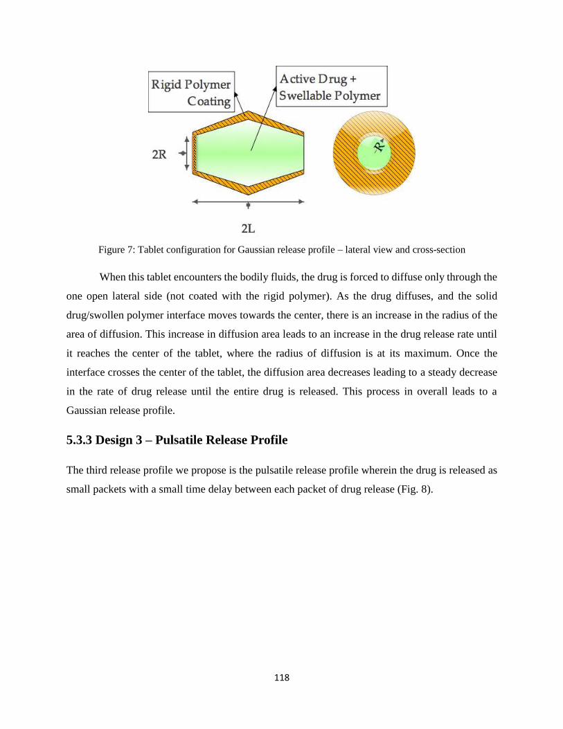
118

Figure 7: Tablet configuration for Gaussian release profile – lateral view and cross-section

When this tablet encounters the bodily fluids, the drug is forced to diffuse only through the

one open lateral side (not coated with the rigid polymer). As the drug diffuses, and the solid

drug/swollen polymer interface moves towards the center, there is an increase in the radius of the

area of diffusion. This increase in diffusion area leads to an increase in the drug release rate until

it reaches the center of the tablet, where the radius of diffusion is at its maximum. Once the

interface crosses the center of the tablet, the diffusion area decreases leading to a steady decrease

in the rate of drug release until the entire drug is released. This process in overall leads to a

Gaussian release profile.

5.3.3 Design 3 – Pulsatile Release Profile

The third release profile we propose is the pulsatile release profile wherein the drug is released as

small packets with a small time delay between each packet of drug release (Fig. 8).

119

Figure 8: Pulsatile Release Profile

For this profile the tablet design is very similar to the design for a constant release profile

(Fig. 5). This is a cylindrical tablet with a thickness of 2L and radius R. This tablet has its curved

surface coated with a rigid polymer as in design 1. One major addition to this design is the pH

sensitive polymer barriers along the length of the cylindrical tablet (Fig. 9).

Figure 9: Tablet configuration for pulsatile release profile – lateral view and cross-section

When this tablet reaches the area in the GI tract with the proper pH, the pH-sensitive

polymer dissolves exposing the drug to the bodily fluids. The drug is then released in a similar

fashion as described above due to polymer swelling, drug diffusion and water diffusion. The pH

120

sensitive barriers arranged at equidistant places along the length of the tablet introduce a time delay

after each packet of drug is released. The delay time can be adjusted by varying the thickness of

the pH sensitive polymer. Through this design a pulsatile release profile is achieved.

5.4 Results and discussions

We used the drug release model discussed in the previous chapters to simulate some profiles that

could be obtained through the tablet configurations proposed in this work. We were able to

successfully simulate a constant release profile (Fig. 10) and a pulsatile release profile (Fig. 11).

Figure 10: Simulated constant release profile for design 1. Constant slope indicates a zero-order release

We observe that the model predicts the initial burst release of the drug followed by a

constant release profile as expected. The total time for drug release can be changed by varying the

121

dissolution rate of the polymer. We simulated a pulsatile release profile as shown in Fig. 11 for

tablet design 3.

Figure 11: Simulated pulsatile release profile for design 3. Time delay indicates the delay between two

consecutive pulse releases

When the first pulse of drug is released, there is a gap before the next pulse as shown in

Fig. 11. There is no drug release during this gap, indicating that degradation of the pH sensitive

polymer barrier is taking place. It is possible to increase or decrease this time gap by

correspondingly changing the thickness of the polymer barrier or by using different polymers with

different dissolution rate constants.

122

5.5 Conclusions

We proposed tablet configurations (dosage form designs) which could potentially lead to desired

drug release profiles such as a constant or zero-order release profile, Gaussian release profile and

a pulsatile release profiles. The proposed configurations are theoretically sound with simple

designs that could be manufactured with little difficulty. The practicality of the designs can only

be ascertained through thorough experiments and availability of the desired polymers for different

applications discussed in this work. These include rigid polymers, swelling polymers and pH

sensitive polymers.

We simulated the release profiles that could be obtained using the drug release model. We

were able to successfully simulate the profiles for constant release and pulsatile release. The

dissolution time of a constant release tablet can be altered by changing the dissolution rate of the

polymer (using different polymers with varying dissolution rate). The time gap between each pulse

release in a pulsatile release profile can be controlled by controlling the thickness of the pH

sensitive barrier and the dissolution rate of the pH sensitive polymer. The total dose of drug can

be varied by varying the drug loading of the tablet. We need a good model to simulate the tablet

design 2, leading to a Gaussian release profile.

A desired drug release profile is inspired by a desired plasma concentration profile or a

desired therapeutic effect. This work inspires the idea of personalized medicine. We will be able

to design tablet configurations based on the requirements of a specific individual patient, his

physiological and genetic makeup, and the desired therapeutic effect. This will greatly improve

the patient compliance, improve the efficiency of the drug tablet, and reduce the dosage frequency.

123

5.6 References

Cobby, J., M. Mayersohn and G. C. Walker (1974). "Influence of shape factors on kinetics of drug

release from matrix tablets I: Theoretical." Journal of pharmaceutical sciences 63(5): 725-732.

Colombo, P. (1993). "Swelling-controlled release in hydrogel matrices for oral route." Advanced

Drug Delivery Reviews 11(1–2): 37-57.

Colombo, P., P. Santi, R. Bettini, O. Strusi, F. Sonvico and G. Colombo (2008). New modules,

new assemblage kits and new assemblies for the controlled release of substances, WO Patent

2,008,067,829.

Ford, J. L., M. H. Rubinstein, F. McCaul, J. E. Hogan and P. J. Edgar (1987). "Importance of drug

type, tablet shape and added diluents on drug release kinetics from hydroxypropylmethylcellulose

matrix tablets." International journal of pharmaceutics 40(3): 223-234.

Huglin, M. R. (1989). "Hydrogels in medicine and pharmacy Edited by N. A. Peppas, CRC Press

Inc., Boca Raton, Florida, 1986 (Vol. l), 1987 (Vols 2 and 3). Vol. 1 Fundamentals, pp. vii + 180,

£72.00, ISBN 0-8493-5546-X; Vol. 2 Polymers, pp. vii + 171, £72.00, ISBN 0-8493-5547-8; Vol.

3 Properties and Applications, pp. vii + 195, £8000, ISBN 0-8493-5548-6." British Polymer

Journal 21(2): 184-184.

Kim, C.-j. (1995). "Compressed donut-shaped tablets with zero-order release kinetics."

Pharmaceutical research 12(7): 1045-1048.

Krögel, I. and R. Bodmeier (1999). "Development of a multifunctional matrix drug delivery

system surrounded by an impermeable cylinder." Journal of controlled release 61(1): 43-50.

Losi, E., R. Bettini, P. Santi, F. Sonvico, G. Colombo, K. Lofthus, P. Colombo and N. A. Peppas

(2006). "Assemblage of novel release modules for the development of adaptable drug delivery

systems." Journal of controlled release 111(1): 212-218.

Losi, E., R. Bettini, P. Santi, F. Sonvico, G. Colombo, K. Lofthus, P. Colombo and N. A. Peppas

(2006). "Assemblage of novel release modules for the development of adaptable drug delivery

systems." Journal of Controlled Release 111(1–2): 212-218.

124

Reynolds, T. D., S. A. Mitchell and K. M. Balwinski (2002). "Investigation of the effect of tablet

surface area/volume on drug release from hydroxypropylmethylcellulose controlled-release matrix

tablets." Drug development and industrial pharmacy 28(4): 457-466.

Sangalli, M. E., A. Maroni, L. Zema, M. Cerea, U. Conte and A. Gazzaniga (2003). "A study on

the release mechanism of drugs from hydrophilic partially coated perforated matrices." Il Farmaco

58(9): 971-976.

Shah, N. H., A. S. Railkar, W. Phuapradit, F.-W. Zeng, A. Chen, M. H. Infeld and A. Malick

(1996). "Effect of processing techniques in controlling the release rate and mechanical strength of

hydroxypropyl methylcellulose based hydrogel matrices." European journal of pharmaceutics and

biopharmaceutics 42(3): 183-187.

Sheskey, P. J. and J. Hendren (1999). "The Effects of Roll Compaction Equipment Variables,

Granulation Technique, and HPMC Polymer Level on Controlled-Release Matrix Model Drug

Formulation." Pharmaceutical technology 23: 90-107.

Siepmann, J., H. Kranz, N. Peppas and R. Bodmeier (2000). "Calculation of the required size and

shape of hydroxypropyl methylcellulose matrices to achieve desired drug release profiles."

International journal of pharmaceutics 201(2): 151-164.

Skoug, J. W., M. T. Borin, J. C. Fleishaker and A. M. Cooper (1991). "In vitro and in vivo

evaluation of whole and half tablets of sustained-release adinazolam mesylate." Pharmaceutical

research 8(12): 1482-1488.

Wesselingh, J. A. and H. W. Frijlink (2008). Mass Transfer from Solid Oral Dosage Forms.

Pharmaceutical Dosage Forms - Tablets, CRC Press: 1-50.

125

CHAPTER 6

Research Summary

In chapter 2, we successfully developed a drug release model to predict the release behavior of

an oral drug from the solid drug tablet inside the GI tract of the body. A solution strategy was

proposed to solve the moving boundary problem encountered in solving the drug release model.

Using this model, we studied the effects of model parameters such as the polymer degradation

rate constant ( dk ), on the tablet dissolution rate. We specifically studied the effect on the

thickness of the solid tablet ( G ) as well as the total tablet including the swollen gel layer ( S ).

The value of G continuously decreased with time, while the value of S initially increased and

then decreased as expected. The profiles indicated a burst release during the initial stages of the

release process.

The solution that we have employed in this model to solve the moving boundary problem

is an approximate solution. There is need for a more efficient solution to the moving boundary

problem that would lead to more accurate predictions. A major assumption in the model is that

the drug release takes place only along the tablet thickness (axial direction) leading to a 2-D

model. We will extend this work by considering the release in all directions (a 3-D model),

which is more realistic but more computationally demanding. The model solution strategy

employed in this work is a discrete approach, where the time and space are divided into small

fractions and the model is solved in each of these fractions. A better solution would be needed.

The developed model will provide insights into the various mass transport, diffusion and

degradation processes involved in the mechanism of drug release from a swelling polymer

matrix. This model will greatly aid in simulating some of the in vitro dissolution tests and reduce

the number of experiments, and hence reduce the time and effort involved.

In chapter 3, we successfully developed a pharmacokinetic model incorporating the drug

release, transit, absorption and elimination processes inside the GI tract of the human body. The

advantage of the suggested approach is that it can be used to test hypothesis about the

mechanism involved in drug delivery into the blood circulatory system. The model is very

flexible and can be applied to different patients with varying body weights. We incorporated the

126

model within an optimization framework to estimate the optimal geometry of the tablet, which

will give the maximum efficacy.

This pharmacokinetic model is based on the ACAT model, which represents the GI tract

as a series of well-mixed continuous stirred tanks (CSTR’s); however, the GI tract is a

continuous tube more closely represented by for example by a piece-wise tubular vessel with

constant cross section and axial dispersion. We are pursuing this angle as well with the

understanding that higher model complexity and model accuracy would result. The tubular flow

model would account for spatial variation of drug concentration inside the compartments. We

plan to extend the model to allow it to predict a plasma profile of a general shape. This will make

it possible to design the optimal dosage form and optimal dosage regimen to obtain a desired

plasma profile in a desired shape. The model can be extended for predicting drug behavior in

model animals such as rats and dogs by adapting the model to represent the physiology. This will

be greatly beneficial to the pharmaceutical industry in performing animal studies and help in

reducing the number of test subjects.

In chapter 4, we used a CAMD framework to generate molecular structures of polymers

with desired properties. We have successfully generated molecular structures of repeat units of

polymers that have the potential to be used as efficient carrier materials for drug delivery. We

discussed an efficient methodology to rank the generated polymers based on their desirability.

The higher their desirability value, the more useful is the polymer for the intended application.

We discussed a method to filter out the polymer candidates based on their compatibility with the

available pharmaceutical drugs. We used solubility parameter analysis to determine the

compatibility between a polymer and a drug.

In the CAMD methodology, we used a group contribution method to predict polymer

properties such as glass transition temperature ( gT ), expansion coefficient ( f ) and water

absorption (W ). A mixed integer nonlinear optimization technique was used to successfully

generate some novel polymer structures. There is a limited availability of group contribution

parameters to only some polymer properties. We plan to extend this work by developing group

contribution parameters for other desired polymer properties such as diffusion coefficients of

water and drug in the polymer and porosity of the polymer. We designed simple homopolymers

127

in this work. It would be a value addition to extend the work to design co-polymers satisfying

desired property constraints. This work deals with generating polymer repeat units by linear

arrangement of the identified groups. It would be interesting to incorporate side chain formation

in the design of the polymer.

The generated molecular structures using this methodology need further analysis and

investigation for them to be practically used for drug delivery applications. An expert opinion

from a polymer chemist about the validity of the generated structures is very essential. An

opinion about the possibility of synthesizing the new polymers, the practicality and economics

involved, will greatly help in progress of this work. The developed CAMD methodology greatly

helps in the product development process by reducing the number of experimental trials, hence

reducing the time and effort involved. It helps in identifying potential failures in the early

development process, thereby avoiding late stage failures, which tend to be very expensive.

In chapter 5, we proposed tablet configurations (dosage form designs) which could

potentially lead to desired drug release profiles such as a constant or zero-order release profile,

Gaussian release profile and a pulsatile release profiles. The proposed configurations are

theoretically sound with simple designs which could be manufactured with little difficulty. The

practicality of the designs can only be ascertained through thorough experiments and availability

of the desired polymers for different applications discussed in this work. These include rigid

polymers, swelling polymers and pH sensitive polymers.

A desired drug release profile is inspired by a desired plasma concentration profile or a

desired therapeutic effect. This work inspires the idea of personalized medicine. We will be able

to design tablet configurations based on the requirements of a specific individual patient, his

physiological and genetic makeup, and the desired therapeutic effect. This will greatly improve

the patient compliance, improve the efficiency of the drug tablet and reduce the dosage

frequency.

The development of a good modeling platform to predict the behavior of drug inside the

body facilitates the drug development and design process. It helps in selecting the most favorable

candidates for the drug development based on the desired properties and greatly reduces the

number of experiments needed for drug development. This further reduces the time and effort

128

required significantly. It aids in reducing the dependence on trial-and-error methods used for

drug development and design. The developed model follows a two-way approach i.e., given the

drug tablet; it can predict the plasma concentration profile and evaluate the pharmacokinetic

parameters like peak plasma concentration, area under the curve and bioavailability. Given the

target plasma profile or the corresponding pharmacokinetic parameters, the model can evaluate

the optimal design parameters of the drug tablet. This research will greatly aid in the

development of personalized medicine, which is the future of drug industry. Personalized

medicine is the development of specific drug for specific patient based on individual’s

physiology and genetic makeup. These personalized drugs will be more effective for each

individual, since right amount of drug will be given to the patient at the right time with

maximum efficiency.

Many advanced models have been developed and are being developed to predict the release of

drug from a polymer matrix system. Many of these models have increased in complexity and

have become more accurate due to improvement in the simulation programs that are being used

to solve the underlying mathematical problems. It would be very useful to understand and model

the effect of different kinds of excipients on the drug release behavior. The modeling framework

developed is more focused on the macroscopic environment of the GI tract in the human body.

The model is useful to predict the amount of drug released, absorbed and eliminated. However,

we did not focus on the microscopic environment such as, the different processes through with

the drug absorption takes place, or the different processes through which drug elimination takes

place. Much more advanced models are available which focus more on these microscopic

processes in detail. Our model can be modified to include these microscopic process based on the

requirement of the client. It would also be very useful to modify the current model using

physiologically based pharmacokinetic (PBPK) modeling to be used for pharmacokinetic studies

in animals such as rats and dogs. The current model has the ability to be used along with or

combine with other models to further enhance the predictability and usability. This could have a

significant impact by saving a lot of time and money during animal studies. The molecular

design framework using group contributions is a simple method to design the polymer structures.

The uncertainties involved in the group contribution parameters make the CAMD process less

accurate. Much more advanced property prediction models are available which could be adapted

to make the molecular design more accurate and efficient. The major limitations with the

129

proposed tablet designs are the economics involved in manufacturing these tablets, customized to

each patient. In the current pharmaceutical industry, standard shapes, sizes and dosages of the

oral tablet are used which is much more economical compared to designing individual tablets

specific to each patient. Based on all the recent advances, we can expect a significant

improvement in the development of accurate and efficient computational models for improving

the overall drug discovery and development process.

Documents

ORAL DRUG DELIVERY MOLECULAR DESIGN AND … along with a computer aided technique to generate molecular structures of polymers ... 4.4 Computational Techniques in Computer Aided Molecular