Oracle® Crystal Ball, Fusion Edition · Predictor is an easy-to-use, graphically oriented forecasting feature included in: l Oracle Crystal Ball, Fusion Edition, including Student

Oracle® Crystal Ball, Fusion EditionOracle® Crystal Ball Decision Optimizer, Fusion EditionOracle® Crystal Ball Enterprise Performance Management, Fusion EditionOracle® Crystal Ball Classroom Student Edition, Fusion EditionOracle® Crystal Ball Classroom Faculty Edition, Fusion EditionOracle® Crystal Ball Enterprise Performance Management for Oracle HyperionEnterprise Planning Suite

Predictor User's Guide

RELEASE 11.1.2

Crystal Ball Predictor User's Guide, 11.1.2

Copyright © 1988, 2011, Oracle and/or its affiliates. All rights reserved.

Authors: EPM Information Development Team

This software and related documentation are provided under a license agreement containing restrictions on use anddisclosure and are protected by intellectual property laws. Except as expressly permitted in your license agreement orallowed by law, you may not use, copy, reproduce, translate, broadcast, modify, license, transmit, distribute, exhibit,perform, publish, or display any part, in any form, or by any means. Reverse engineering, disassembly, or decompilationof this software, unless required by law for interoperability, is prohibited. The information contained herein is subject tochange without notice and is not warranted to be error-free. If you find any errors, please report them to us in writing.

If this software or related documentation is delivered to the U.S. Government or anyone licensing it on behalf of the U.S.Government, the following notice is applicable:

U.S. GOVERNMENT RIGHTS:Programs, software, databases, and related documentation and technical data delivered to U.S. Government customersare "commercial computer software" or "commercial technical data" pursuant to the applicable Federal AcquisitionRegulation and agency-specific supplemental regulations. As such, the use, duplication, disclosure, modification, andadaptation shall be subject to the restrictions and license terms set forth in the applicable Government contract, and, tothe extent applicable by the terms of the Government contract, the additional rights set forth in FAR 52.227-19, CommercialComputer Software License (December 2007). Oracle USA, Inc., 500 Oracle Parkway, Redwood City, CA 94065.

This software is developed for general use in a variety of information management applications. It is not developed orintended for use in any inherently dangerous applications, including applications which may create a risk of personalinjury. If you use this software in dangerous applications, then you shall be responsible to take all appropriate fail-safe,backup, redundancy, and other measures to ensure the safe use of this software. Oracle Corporation and its affiliatesdisclaim any liability for any damages caused by use of this software in dangerous applications.

Oracle is a registered trademark of Oracle Corporation and/or its affiliates. Other names may be trademarks of theirrespective owners.

This software and documentation may provide access to or information on content, products, and services from thirdparties. Oracle Corporation and its affiliates are not responsible for and expressly disclaim all warranties of any kind withrespect to third-party content, products, and services. Oracle Corporation and its affiliates will not be responsible for anyloss, costs, or damages incurred due to your access to or use of third-party content, products, or services.

Contents

Chapter 1. Welcome . . . . . . . . . . . . . . . . . . . . . . . . . . . . . . . . . . . . . . . . . . . . . . . . . . . . . . . . . . . . . . . . . 7

About Predictor . . . . . . . . . . . . . . . . . . . . . . . . . . . . . . . . . . . . . . . . . . . . . . . . . . . . . . . 7

How This Guide Is Organized . . . . . . . . . . . . . . . . . . . . . . . . . . . . . . . . . . . . . . . . . . . . . 8

Screen Capture Notes . . . . . . . . . . . . . . . . . . . . . . . . . . . . . . . . . . . . . . . . . . . . . . . . 8

Example Files . . . . . . . . . . . . . . . . . . . . . . . . . . . . . . . . . . . . . . . . . . . . . . . . . . . . . . 8

Online Help . . . . . . . . . . . . . . . . . . . . . . . . . . . . . . . . . . . . . . . . . . . . . . . . . . . . . . . . . . 9

Developer Kit . . . . . . . . . . . . . . . . . . . . . . . . . . . . . . . . . . . . . . . . . . . . . . . . . . . . . . . . . 9

Accessibility Notes . . . . . . . . . . . . . . . . . . . . . . . . . . . . . . . . . . . . . . . . . . . . . . . . . . . . . 9

Additional Resources . . . . . . . . . . . . . . . . . . . . . . . . . . . . . . . . . . . . . . . . . . . . . . . . . . . 9

Chapter 2. Getting Started with Predictor . . . . . . . . . . . . . . . . . . . . . . . . . . . . . . . . . . . . . . . . . . . . . . . . . 11

Forecasting Basics . . . . . . . . . . . . . . . . . . . . . . . . . . . . . . . . . . . . . . . . . . . . . . . . . . . . . 11

Creating Spreadsheets with Historical Data . . . . . . . . . . . . . . . . . . . . . . . . . . . . . . . . . . . 12

Starting Predictor and Running a Forecast . . . . . . . . . . . . . . . . . . . . . . . . . . . . . . . . . . . 13

Analyzing Results at a Basic Level . . . . . . . . . . . . . . . . . . . . . . . . . . . . . . . . . . . . . . . . . . 14

Learning More . . . . . . . . . . . . . . . . . . . . . . . . . . . . . . . . . . . . . . . . . . . . . . . . . . . . . . . 14

Chapter 3. Setting Up Predictor Forecasts . . . . . . . . . . . . . . . . . . . . . . . . . . . . . . . . . . . . . . . . . . . . . . . . . 15

Guidelines for Setting Up a Forecast . . . . . . . . . . . . . . . . . . . . . . . . . . . . . . . . . . . . . . . . 15

Selecting the Location and Arrangement of Historical Data . . . . . . . . . . . . . . . . . . . . . . . 17

Selecting Discontiguous Data . . . . . . . . . . . . . . . . . . . . . . . . . . . . . . . . . . . . . . . . . . 18

Selecting Data Attributes—Seasonality, Events, Screening . . . . . . . . . . . . . . . . . . . . . . . . 19

Viewing Historical Data by Seasonality . . . . . . . . . . . . . . . . . . . . . . . . . . . . . . . . . . . 20

Identifying Seasonality with Autocorrelations . . . . . . . . . . . . . . . . . . . . . . . . . . . 22

Viewing and Managing Events . . . . . . . . . . . . . . . . . . . . . . . . . . . . . . . . . . . . . . . . . 24

Adding Events . . . . . . . . . . . . . . . . . . . . . . . . . . . . . . . . . . . . . . . . . . . . . . . . . 26

Editing Events . . . . . . . . . . . . . . . . . . . . . . . . . . . . . . . . . . . . . . . . . . . . . . . . . 27

Deleting Events . . . . . . . . . . . . . . . . . . . . . . . . . . . . . . . . . . . . . . . . . . . . . . . . . 27

Setting Event Dates . . . . . . . . . . . . . . . . . . . . . . . . . . . . . . . . . . . . . . . . . . . . . . 27

Viewing Screened Data . . . . . . . . . . . . . . . . . . . . . . . . . . . . . . . . . . . . . . . . . . . . . . 28

Setting Screening Options . . . . . . . . . . . . . . . . . . . . . . . . . . . . . . . . . . . . . . . . . . . . 28

Selecting a Forecasting Method . . . . . . . . . . . . . . . . . . . . . . . . . . . . . . . . . . . . . . . . . . . 29

Contents iii

Using Classic Time-series Forecasting Methods . . . . . . . . . . . . . . . . . . . . . . . . . . . . . 30

Setting Classic Time-series Forecasting Method Parameters . . . . . . . . . . . . . . . . . 32

Using ARIMA Time-series Forecasting Methods . . . . . . . . . . . . . . . . . . . . . . . . . . . . 33

Selecting an ARIMA Model Selection Criterion . . . . . . . . . . . . . . . . . . . . . . . . . . 34

Using ARIMA Custom Models . . . . . . . . . . . . . . . . . . . . . . . . . . . . . . . . . . . . . 35

Adding Custom ARIMA Models . . . . . . . . . . . . . . . . . . . . . . . . . . . . . . . . . . . . 35

Editing Custom ARIMA Models . . . . . . . . . . . . . . . . . . . . . . . . . . . . . . . . . . . . 36

Setting ARIMA Options . . . . . . . . . . . . . . . . . . . . . . . . . . . . . . . . . . . . . . . . . . 36

Using Multiple Linear Regression . . . . . . . . . . . . . . . . . . . . . . . . . . . . . . . . . . . . . . . 37

Selecting Regression Variables . . . . . . . . . . . . . . . . . . . . . . . . . . . . . . . . . . . . . . 38

Setting Stepwise Regression Options . . . . . . . . . . . . . . . . . . . . . . . . . . . . . . . . . 38

Setting Forecast Options . . . . . . . . . . . . . . . . . . . . . . . . . . . . . . . . . . . . . . . . . . . . . . . . 39

Selecting Error Measures . . . . . . . . . . . . . . . . . . . . . . . . . . . . . . . . . . . . . . . . . . . . . 39

Selecting Forecasting Techniques . . . . . . . . . . . . . . . . . . . . . . . . . . . . . . . . . . . . . . . 40

Chapter 4. Analyzing Predictor Results . . . . . . . . . . . . . . . . . . . . . . . . . . . . . . . . . . . . . . . . . . . . . . . . . . . 41

Understanding the Predictor Results Window . . . . . . . . . . . . . . . . . . . . . . . . . . . . . . . . . 41

Entering the Number of Time Periods to Forecast . . . . . . . . . . . . . . . . . . . . . . . . . . . 43

Selecting a Confidence Interval . . . . . . . . . . . . . . . . . . . . . . . . . . . . . . . . . . . . . . . . 43

Selecting How to Display and Analyze Results . . . . . . . . . . . . . . . . . . . . . . . . . . . . . . . . . 44

Adjusting Forecasted Data . . . . . . . . . . . . . . . . . . . . . . . . . . . . . . . . . . . . . . . . . . . . . . . 44

Custom Rounding . . . . . . . . . . . . . . . . . . . . . . . . . . . . . . . . . . . . . . . . . . . . . . . . . 45

Pasting Predictor Forecasts . . . . . . . . . . . . . . . . . . . . . . . . . . . . . . . . . . . . . . . . . . . . . . 46

Time-series Forecast Method Results . . . . . . . . . . . . . . . . . . . . . . . . . . . . . . . . . . . . 47

Multiple Linear Regression Results . . . . . . . . . . . . . . . . . . . . . . . . . . . . . . . . . . . . . . 47

Viewing Charts . . . . . . . . . . . . . . . . . . . . . . . . . . . . . . . . . . . . . . . . . . . . . . . . . . . . . . . 47

Customizing Charts . . . . . . . . . . . . . . . . . . . . . . . . . . . . . . . . . . . . . . . . . . . . . . . . 48

Copying and Printing Charts . . . . . . . . . . . . . . . . . . . . . . . . . . . . . . . . . . . . . . . . . . 49

Creating Reports . . . . . . . . . . . . . . . . . . . . . . . . . . . . . . . . . . . . . . . . . . . . . . . . . . . . . . 49

Extracting Results Data . . . . . . . . . . . . . . . . . . . . . . . . . . . . . . . . . . . . . . . . . . . . . . . . . 50

Analyzing and Using Extracted Results . . . . . . . . . . . . . . . . . . . . . . . . . . . . . . . . . . . 51

Appendix A. Predictor Tutorials . . . . . . . . . . . . . . . . . . . . . . . . . . . . . . . . . . . . . . . . . . . . . . . . . . . . . . . . 53

About Predictor Tutorials . . . . . . . . . . . . . . . . . . . . . . . . . . . . . . . . . . . . . . . . . . . . . . . 53

Tutorial 1—Shampoo Sales . . . . . . . . . . . . . . . . . . . . . . . . . . . . . . . . . . . . . . . . . . . . . . 53

Tutorial 2—Toledo Gas . . . . . . . . . . . . . . . . . . . . . . . . . . . . . . . . . . . . . . . . . . . . . . . . . 57

Viewing and Analyzing Predictor Results . . . . . . . . . . . . . . . . . . . . . . . . . . . . . . . . . 59

Pasting Results into the Spreadsheet . . . . . . . . . . . . . . . . . . . . . . . . . . . . . . . . . . . . . 62

Creating a Report of Predictor Results . . . . . . . . . . . . . . . . . . . . . . . . . . . . . . . . . . . 64

Extracting Results . . . . . . . . . . . . . . . . . . . . . . . . . . . . . . . . . . . . . . . . . . . . . . . . . . 65

iv Contents

Working with Data in Interactive Tables . . . . . . . . . . . . . . . . . . . . . . . . . . . . . . . 66

Appendix B. Predictor Examples . . . . . . . . . . . . . . . . . . . . . . . . . . . . . . . . . . . . . . . . . . . . . . . . . . . . . . . . 71

About These Examples . . . . . . . . . . . . . . . . . . . . . . . . . . . . . . . . . . . . . . . . . . . . . . . . . 71

Inventory Control . . . . . . . . . . . . . . . . . . . . . . . . . . . . . . . . . . . . . . . . . . . . . . . . . . . . . 72

Company Finances . . . . . . . . . . . . . . . . . . . . . . . . . . . . . . . . . . . . . . . . . . . . . . . . . . . . 74

Human Resources . . . . . . . . . . . . . . . . . . . . . . . . . . . . . . . . . . . . . . . . . . . . . . . . . . . . . 77

Appendix C. Important Predictor Concepts . . . . . . . . . . . . . . . . . . . . . . . . . . . . . . . . . . . . . . . . . . . . . . . . 81

About Forecasting Concepts . . . . . . . . . . . . . . . . . . . . . . . . . . . . . . . . . . . . . . . . . . . . . 81

Classic Time-series Forecasting . . . . . . . . . . . . . . . . . . . . . . . . . . . . . . . . . . . . . . . . . . . 82

Classic Non-seasonal Forecasting Methods . . . . . . . . . . . . . . . . . . . . . . . . . . . . . . . . 83

Single Moving Average (SMA) . . . . . . . . . . . . . . . . . . . . . . . . . . . . . . . . . . . . . . 83

Double Moving Average (DMA) . . . . . . . . . . . . . . . . . . . . . . . . . . . . . . . . . . . . 83

Single Exponential Smoothing (SES) . . . . . . . . . . . . . . . . . . . . . . . . . . . . . . . . . 84

Double Exponential Smoothing (DES) . . . . . . . . . . . . . . . . . . . . . . . . . . . . . . . . 84

Classic Non-seasonal Forecasting Method Parameters . . . . . . . . . . . . . . . . . . . . . 85

Classic Seasonal Forecasting Methods . . . . . . . . . . . . . . . . . . . . . . . . . . . . . . . . . . . . 85

Seasonal Additive . . . . . . . . . . . . . . . . . . . . . . . . . . . . . . . . . . . . . . . . . . . . . . . 86

Seasonal Multiplicative . . . . . . . . . . . . . . . . . . . . . . . . . . . . . . . . . . . . . . . . . . . 86

Holt-Winters’ Additive . . . . . . . . . . . . . . . . . . . . . . . . . . . . . . . . . . . . . . . . . . . 86

Holt-Winters’ Multiplicative . . . . . . . . . . . . . . . . . . . . . . . . . . . . . . . . . . . . . . . 87

Classic Seasonal Forecasting Method Parameters . . . . . . . . . . . . . . . . . . . . . . . . . 87

Time-series Forecasting Accuracy Measures . . . . . . . . . . . . . . . . . . . . . . . . . . . . . . . . . . 88

RMSE . . . . . . . . . . . . . . . . . . . . . . . . . . . . . . . . . . . . . . . . . . . . . . . . . . . . . . . . . . 89

MAD . . . . . . . . . . . . . . . . . . . . . . . . . . . . . . . . . . . . . . . . . . . . . . . . . . . . . . . . . . . 89

MAPE . . . . . . . . . . . . . . . . . . . . . . . . . . . . . . . . . . . . . . . . . . . . . . . . . . . . . . . . . . 89

Theil’s U . . . . . . . . . . . . . . . . . . . . . . . . . . . . . . . . . . . . . . . . . . . . . . . . . . . . . . . . 89

Durbin-Watson . . . . . . . . . . . . . . . . . . . . . . . . . . . . . . . . . . . . . . . . . . . . . . . . . . . 89

Time-series Forecasting Techniques . . . . . . . . . . . . . . . . . . . . . . . . . . . . . . . . . . . . . . . . 90

Standard Forecasting . . . . . . . . . . . . . . . . . . . . . . . . . . . . . . . . . . . . . . . . . . . . . . . . 90

Simple Lead Forecasting . . . . . . . . . . . . . . . . . . . . . . . . . . . . . . . . . . . . . . . . . . . . . 91

Weighted Lead Forecasting . . . . . . . . . . . . . . . . . . . . . . . . . . . . . . . . . . . . . . . . . . . 91

Holdout Forecasting . . . . . . . . . . . . . . . . . . . . . . . . . . . . . . . . . . . . . . . . . . . . . . . . 91

Multiple Linear Regression . . . . . . . . . . . . . . . . . . . . . . . . . . . . . . . . . . . . . . . . . . . . . . 92

Regression Methods . . . . . . . . . . . . . . . . . . . . . . . . . . . . . . . . . . . . . . . . . . . . . . . . . . . 93

Standard Regression . . . . . . . . . . . . . . . . . . . . . . . . . . . . . . . . . . . . . . . . . . . . . . . . 93

Forward Stepwise Regression . . . . . . . . . . . . . . . . . . . . . . . . . . . . . . . . . . . . . . . . . . 93

Iterative Stepwise Regression . . . . . . . . . . . . . . . . . . . . . . . . . . . . . . . . . . . . . . . . . . 94

Regression Statistics . . . . . . . . . . . . . . . . . . . . . . . . . . . . . . . . . . . . . . . . . . . . . . . . . . . 95

Contents v

R2 . . . . . . . . . . . . . . . . . . . . . . . . . . . . . . . . . . . . . . . . . . . . . . . . . . . . . . . . . . . . . 95

Adjusted R2 . . . . . . . . . . . . . . . . . . . . . . . . . . . . . . . . . . . . . . . . . . . . . . . . . . . . . . 95

Sum of Squared Errors (SSE) . . . . . . . . . . . . . . . . . . . . . . . . . . . . . . . . . . . . . . . . . . 95

F statistic . . . . . . . . . . . . . . . . . . . . . . . . . . . . . . . . . . . . . . . . . . . . . . . . . . . . . . . . 96

t statistic . . . . . . . . . . . . . . . . . . . . . . . . . . . . . . . . . . . . . . . . . . . . . . . . . . . . . . . . . 96

p . . . . . . . . . . . . . . . . . . . . . . . . . . . . . . . . . . . . . . . . . . . . . . . . . . . . . . . . . . . . . . 96

Historical Data Statistics . . . . . . . . . . . . . . . . . . . . . . . . . . . . . . . . . . . . . . . . . . . . . . . . 96

Mean . . . . . . . . . . . . . . . . . . . . . . . . . . . . . . . . . . . . . . . . . . . . . . . . . . . . . . . . . . . 96

Standard Deviation . . . . . . . . . . . . . . . . . . . . . . . . . . . . . . . . . . . . . . . . . . . . . . . . . 97

Minimum . . . . . . . . . . . . . . . . . . . . . . . . . . . . . . . . . . . . . . . . . . . . . . . . . . . . . . . 97

Maximum . . . . . . . . . . . . . . . . . . . . . . . . . . . . . . . . . . . . . . . . . . . . . . . . . . . . . . . 97

Ljung-Box Statistic . . . . . . . . . . . . . . . . . . . . . . . . . . . . . . . . . . . . . . . . . . . . . . . . . 97

Data Screening and Adjustment Methods . . . . . . . . . . . . . . . . . . . . . . . . . . . . . . . . . . . . 97

Outlier Detection Methods . . . . . . . . . . . . . . . . . . . . . . . . . . . . . . . . . . . . . . . . . . . 97

Mean and Standard Deviation Method . . . . . . . . . . . . . . . . . . . . . . . . . . . . . . . . 98

Median and Median Absolute Deviation Method (MAD) . . . . . . . . . . . . . . . . . . 98

Median and Interquartile Deviation Method (IQD) . . . . . . . . . . . . . . . . . . . . . . 98

Outlier and Missing Value Adjustment Methods . . . . . . . . . . . . . . . . . . . . . . . . . . . . 99

Cubic Spline Interpolation Method . . . . . . . . . . . . . . . . . . . . . . . . . . . . . . . . . . 99

Neighbor Interpolation Method . . . . . . . . . . . . . . . . . . . . . . . . . . . . . . . . . . . . . 99

Appendix D. Bibliography . . . . . . . . . . . . . . . . . . . . . . . . . . . . . . . . . . . . . . . . . . . . . . . . . . . . . . . . . . . 101

Forecasting . . . . . . . . . . . . . . . . . . . . . . . . . . . . . . . . . . . . . . . . . . . . . . . . . . . . . . . . . 101

ARIMA Forecasting . . . . . . . . . . . . . . . . . . . . . . . . . . . . . . . . . . . . . . . . . . . . . . . . . . 101

Regression Analysis . . . . . . . . . . . . . . . . . . . . . . . . . . . . . . . . . . . . . . . . . . . . . . . . . . . 102

Glossary . . . . . . . . . . . . . . . . . . . . . . . . . . . . . . . . . . . . . . . . . . . . . . . . . . . . . . . . . . . . . . . . . . . . . . . 103

Index . . . . . . . . . . . . . . . . . . . . . . . . . . . . . . . . . . . . . . . . . . . . . . . . . . . . . . . . . . . . . . . . . . . . . . . . . 107

vi Contents

1Welcome

In This Chapter

About Predictor.. . . . . . . . . . . . . . . . . . . . . . . . . . . . . . . . . . . . . . . . . . . . . . . . . . . . . . . . . . . . . . . . . . . . . . . . . . . . . . . . . . . . . . . . . . . . . 7

How This Guide Is Organized... . . . . . . . . . . . . . . . . . . . . . . . . . . . . . . . . . . . . . . . . . . . . . . . . . . . . . . . . . . . . . . . . . . . . . . . . . . . . 8

Online Help ... . . . . . . . . . . . . . . . . . . . . . . . . . . . . . . . . . . . . . . . . . . . . . . . . . . . . . . . . . . . . . . . . . . . . . . . . . . . . . . . . . . . . . . . . . . . . . . . 9

Developer Kit . . . . . . . . . . . . . . . . . . . . . . . . . . . . . . . . . . . . . . . . . . . . . . . . . . . . . . . . . . . . . . . . . . . . . . . . . . . . . . . . . . . . . . . . . . . . . . . . 9

Accessibility Notes ... . . . . . . . . . . . . . . . . . . . . . . . . . . . . . . . . . . . . . . . . . . . . . . . . . . . . . . . . . . . . . . . . . . . . . . . . . . . . . . . . . . . . . . . 9

Additional Resources ... . . . . . . . . . . . . . . . . . . . . . . . . . . . . . . . . . . . . . . . . . . . . . . . . . . . . . . . . . . . . . . . . . . . . . . . . . . . . . . . . . . . . 9

About PredictorForecasting is an important part of many business decisions. Every organization must set goals,try to predict future events, and then act to fulfill the goals. As the timeliness of market actionsbecomes more important, the need for accurate planning and forecasting throughout anorganization is essential to get ahead. The difference between good and bad forecasting can affectthe success of an entire organization.

Predictor is an easy-to-use, graphically oriented forecasting feature included in:

l Oracle Crystal Ball, Fusion Edition, including Student and Faculty Editions

l Oracle Crystal Ball Decision Optimizer, Fusion Edition

l Oracle Crystal Ball Enterprise Performance Management, Fusion Edition

If you have historical data in your spreadsheet model, Predictor analyzes the data for trends andseasonal variations. It then predicts future values based on this information. You can answerquestions such as, “What are the likely sales figures for next quarter?” or, “How much materialdo we need to have on hand?” As an added benefit, you can automatically save Predictor forecastsas Crystal Ball assumptions for immediate use in powerful risk analysis models. See Chapter 2,“Getting Started with Predictor,” for an overview of how Predictor works and what it can do foryou.

Predictor runs on several versions of Microsoft Windows and Microsoft Excel. For a list ofrequired hardware and software, see the current Oracle Crystal Ball Installation and LicensingGuide.

About Predictor 7

How This Guide Is OrganizedThis guide includes the following additional sections to help you use Predictor:

l Chapter 2, “Getting Started with Predictor”

Procedures for starting Predictor and running basic forecasts using default settings

l Chapter 3, “Setting Up Predictor Forecasts”

Procedures for running forecasts with customized settings

l Chapter 4, “Analyzing Predictor Results”

Descriptions of Predictor results and how to analyze them

l Appendix A, “Predictor Tutorials”

A basic tutorial that quickly introduces Predictor’s features and an advanced tutorial thatuses multiple regression analysis

l Appendix B, “Predictor Examples”

Forecasting examples from various fields

l Appendix C, “Important Predictor Concepts”

Definitions of important forecasting and statistical terms as they are used in Predictor

l Appendix D, “Bibliography”

A list of related publications for further study

l Glossary

Definitions of terms specific to Predictor as well as statistical terms used in this manual

Screen Capture NotesThe screen captures in this manual were taken in Microsoft Excel 2003 for Microsoft WindowsXP Professional.

Because of round-off differences between various system configurations, you might noticecalculated results that are slightly different from those in the examples.

Example FilesExample names are listed in full wherever given.

ä To open an example file:

1 Select Help, then Crystal Ball, and then Examples Guide.

2 Click its name in the Model Name list. (In Microsoft Excel 2007 or later, select Resources in the Helpgroup, and then select Examples Guide.)

8 Welcome

Online HelpYou can display online help for Predictor by pressing F1 or clicking Help in the Predictor wizard.

Tip: Click Contents at the top of the help window for a table of contents.

Developer KitIf you are familiar with Visual Basic for Applications (VBA) or other supported developmentsystems, you can use the Predictor developer kit to automate a number of basic forecasting andanalysis operations. For details, see the Oracle Crystal Ball Developer's Guide.

Accessibility NotesYou do not need to enable keyboard accessibility specifically for Crystal Ball and its features;command access is always in accessible mode. Crystal Ball, including Predictor, followsMicrosoft Windows conventions for accessing commands using the keyboard. When you pressAlt, shortcut keys are underlined in menus and dialogs. Crystal Ball output can be extracted toMicrosoft Excel spreadsheets and pasted into PowerPoint slides, which are accessible throughMicrosoft Office. Starting with Crystal Ball version 11.1.2.0.00, an optional Accessibility mode,available through the Options tab of the Run Preferences dialog, activates special features forpeople with visual or motor impairments. For example, default chart display includes distinctionby patterns as well as colors. For additional information about Crystal Ball accessibility, see theOracle Crystal Ball User's Guide. For information about Microsoft Excel or PowerPointaccessibility, refer to Microsoft Office product documentation.

Additional ResourcesOracle offers technical support, training, and other services to help you use Crystal Ball mosteffectively.

For more information, see the Crystal Ball Web site at:

http://www.oracle.com/crystalball

Online Help 9

10 Welcome

2Getting Started with Predictor

In This Chapter

Forecasting Basics ... . . . . . . . . . . . . . . . . . . . . . . . . . . . . . . . . . . . . . . . . . . . . . . . . . . . . . . . . . . . . . . . . . . . . . . . . . . . . . . . . . . . . . .11

Creating Spreadsheets with Historical Data ... . . . . . . . . . . . . . . . . . . . . . . . . . . . . . . . . . . . . . . . . . . . . . . . . . . . . . . . . . .12

Starting Predictor and Running a Forecast .. . . . . . . . . . . . . . . . . . . . . . . . . . . . . . . . . . . . . . . . . . . . . . . . . . . . . . . . . . . . .13

Analyzing Results at a Basic Level .. . . . . . . . . . . . . . . . . . . . . . . . . . . . . . . . . . . . . . . . . . . . . . . . . . . . . . . . . . . . . . . . . . . . . .14

Learning More ... . . . . . . . . . . . . . . . . . . . . . . . . . . . . . . . . . . . . . . . . . . . . . . . . . . . . . . . . . . . . . . . . . . . . . . . . . . . . . . . . . . . . . . . . . . .14

Forecasting BasicsMost historical or time-based data contains an underlying trend or seasonal pattern. However,most historical data also contains random fluctuations (“noise”) that make it difficult to detectthese trends and patterns without a computer. Predictor uses sophisticated time-series methodsto analyze the underlying structure of the data. It then projects the trends and patterns to predictfuture values.

Predictor uses two types of forecasting:

l “Classic Time-series Forecasting” on page 82 breaks historical data into components: level,trend, seasonality, and error. Predictor analyzes these components and then projects theminto the future to predict likely results.

l “Multiple Linear Regression” on page 92 works best when outside influences have an effecton the variable that you want to forecast. Regression takes historical data from theinfluencing variables and determines the mathematical relationship between these variablesand the target variable. It then uses time-series forecasting methods to forecast theinfluencing variables and combines the results mathematically to forecast the target variable.

In Predictor, a data series is a set of historical data for a single variable. When you run Predictor,it uses each time-series method on each of the selected data series and calculates a mathematicalmeasure of goodness-of-fit. Predictor selects the method with the best goodness-of-fit as themethod that will yield the most accurate forecast. Predictor performs this selectionautomatically, but you can also select individual methods manually or override the method thatPredictor recommends with a different one.

The final forecast shows the most likely continuation of the data. Keep in mind that all thesemethods assume that some aspects of the historical trend or pattern will continue into the future.However, the farther out you forecast, the greater the likelihood that events will diverge frompast behavior, and the less confident you can be of the results. To help you gauge the reliability

Forecasting Basics 11

of the forecast, Predictor provides a confidence interval indicating the degree of uncertaintyregarding the forecast.

After finding the best forecast for the data, Predictor displays detailed output that can includestatistics, charts, reports, and interactive Microsoft Excel PivotTables. Predictor can also pastethe forecasted values into a spreadsheet and create Crystal Ball assumptions from forecastedvalues so you can perform a “what-if” simulation.

The following topics describe how to set up Predictor forecasts using default settings so you cangenerate results quickly for further analysis:

l “Creating Spreadsheets with Historical Data” on page 12

l “Starting Predictor and Running a Forecast” on page 13

l “Analyzing Results at a Basic Level” on page 14

l “Learning More” on page 14

Predictor basics are demonstrated in “Tutorial 1—Shampoo Sales” on page 53. You may findit helpful to work through this tutorial now, or read through the following sections first andthen try the tutorial. When you are ready to expand your forecasting skills, Chapter 3, “SettingUp Predictor Forecasts,” provides detailed instructions.

Creating Spreadsheets with Historical DataBefore using Predictor, create a Microsoft Excel spreadsheet with historical data to analyze. Thespreadsheet should include:

l Optional: A descriptive spreadsheet title.

l Optional: A date (or other time period, such as Q2-2004) column or row, either at the topor along the left side of the data (in the last column before the data). If you format the datesas Microsoft Excel dates, Predictor can find the dates, extend them with the forecasted values,and use them as chart labels.

l Historical data, spaced equal time periods apart, in columns or rows adjacent to the datecolumn or row. To produce a reasonable forecast, you should have at least six historical datapoints. Other requirements:

m Single moving average analysis requires that the number of historical data points betwice the number of points to forecast.

m Double moving average analysis requires that the number of historical data points bethree times the number of points to forecast (or at least six, whichever is higher).

m To use seasonal methods, you must have at least two seasons (complete cycles) ofhistorical data.

m For multiple linear regression, the number of historical data points must be greater thanor equal to the number of independent variables (counting the included constant as anindependent variable).

12 Getting Started with Predictor

m To lag an independent variable in multiple linear regression, lag must be less than thenumber of historical data points. For details on lags, see “Notes about Autocorrelations”on page 23.

m For multiple linear regression with lags, the number of data points minus any lags andleading blanks must be greater than the number of independent variables, plus 1 if aconstant is included in the regression equation.

m When values in the date series are not in Microsoft Excel date format, the intervalsbetween the values must all be exactly the same. For example, you can use integers forweeks (1, 2, 3, and so on) but you cannot omit any. The following is not an acceptabledata series: 1, 2, 3, 5, 7. Also consider the valid date series 01-Jan, 01-Feb, 01-Mar. Thisis no longer valid when converted into days expressed as integers: 1, 32, 60.

l Optional: Headings for each data column or row, such as SKU 23442, Gas Usage, or InterestRate.

The Toledo Gas spreadsheet (Figure 1) has all these components.

Figure 1 Example Spreadsheet

Starting Predictor and Running a Forecast

ä Before you start Predictor:

1 Open a model with historical data (see “Creating Spreadsheets with Historical Data” on page 12).

2 Select a cell within the range to analyze.

Starting Predictor and Running a Forecast 13

ä To start Predictor:

1 Select Run, and then Predictor.

The first time you start Predictor, the Predictor wizard Welcome panel opens. After that,Input Data opens.

The Welcome panel introduces Predictor and provides an overview of how it works.

2 If Welcome opens, click Next to advance to Input Data.

3 Set up a forecast following the instructions in Chapter 3, “Setting Up Predictor Forecasts.” To set up abasic forecast, see “Guidelines for Setting Up a Forecast” on page 15.

4 To run a forecast and produce results, click Run.

The Predictor Results window opens.

Note: You can click Run from any of the wizard panels except Welcome at any time, as long asthe data range has been properly defined on the Input Data panel.

To use forecasted results, see “Analyzing Results at a Basic Level” on page 14.

Analyzing Results at a Basic LevelPredictor simplifies the forecasting process, but you must understand the results it produces.

For a detailed description of all results and how to analyze them, see Chapter 4, “AnalyzingPredictor Results.” At a basic level, you can view results for different series and paste results intothe spreadsheet model:

l “Understanding the Predictor Results Window” on page 41

l “Entering the Number of Time Periods to Forecast” on page 43

l “Selecting How to Display and Analyze Results” on page 44

Learning MoreThis chapter introduced Predictor at a basic level and suggested topics with more advancedcontent. If you have not already done so, you may find it helpful to:

l Work through “Tutorial 1—Shampoo Sales” on page 53

l Consider reviewing Chapter 3, “Setting Up Predictor Forecasts,” to learn procedures forincreasing the accuracy of Predictor forecasting and analysis

14 Getting Started with Predictor

3Setting Up Predictor Forecasts

In This Chapter

Guidelines for Setting Up a Forecast .. . . . . . . . . . . . . . . . . . . . . . . . . . . . . . . . . . . . . . . . . . . . . . . . . . . . . . . . . . . . . . . . . . . .15

Selecting the Location and Arrangement of Historical Data ... . . . . . . . . . . . . . . . . . . . . . . . . . . . . . . . . . . . . . . . .17

Selecting Data Attributes—Seasonality, Events, Screening ... . . . . . . . . . . . . . . . . . . . . . . . . . . . . . . . . . . . . . . . . .19

Selecting a Forecasting Method ... . . . . . . . . . . . . . . . . . . . . . . . . . . . . . . . . . . . . . . . . . . . . . . . . . . . . . . . . . . . . . . . . . . . . . . .29

Setting Forecast Options ... . . . . . . . . . . . . . . . . . . . . . . . . . . . . . . . . . . . . . . . . . . . . . . . . . . . . . . . . . . . . . . . . . . . . . . . . . . . . . . .39

Guidelines for Setting Up a Forecast

Tip: To preview these steps, work through “Tutorial 1—Shampoo Sales” on page 53.

ä Follow these steps to set up a Predictor forecast and generate results:

1 Create and open a spreadsheet model with historical data as described in “Creating Spreadsheets withHistorical Data” on page 12.

2 Select a data cell and start Predictor (see “Starting Predictor and Running a Forecast” on page 13).

Note: You can select an entire data range or a single cell and let Predictor determine therange. If columns or rows of data are separated by blank columns or rows, you canuse Ctrl+click to select one cell in each data series. For details, see “SelectingDiscontiguous Data” on page 18.

3 Display the Input Data panel of the Predictor wizard.

If Welcome opens, click Next to display Input Data.

4 In Input Data, confirm that:

l The appropriate data range is selected, including any row labels and column headers

l Column Header and Label settings are correct

For details, click Help or see “Selecting the Location and Arrangement of HistoricalData” on page 17.

5 Click Next to display Data Attributes.

6 In Data Attributes, indicate the time period for the data.

For example, if the data points represent monthly numbers, select months.

Guidelines for Setting Up a Forecast 15

7 For Seasonality, select AutoDetect so Predictor will use statistical algorithms to determine whether thedata is seasonal. Findings appear in a statement to the right of the list box. To fine-tune seasonalitysettings or use optional events and screening settings, see “Selecting Data Attributes—Seasonality,Events, Screening” on page 19.

8 Optional: If you are analyzing more than one data series with AutoDetect, click View Seasonality to chartthe seasonality for each series.

For more information, see “Viewing Historical Data by Seasonality” on page 20.

9 Click Next to open the Methods panel, and select forecasting methods.

10 Depending on the Data Attributes Seasonality setting, select one or more of these:

l Non-seasonal Methods—Work best on data that does not show a pattern that repeatsregularly over a certain number of time periods, but can show a trend of decreasing orincreasing over time

l Seasonal Methods—Work best on data that shows a pattern that repeats regularly overa certain number of time periods and can also show a trend of decreasing or increasingover time

l ARIMA—Useful in a variety of situations, particularly when there are many historicalvalues and very few outlier values

l Multiple Linear Regression—Useful when independent variables affect another variableof interest

Tip: If Non-seasonal Methods and Seasonal Methods are available, select both.

If you have selected several series and one of them is controlled by the other, it is a dependentvariable. In that case, select Multiple Linear Regression and see “Using Multiple LinearRegression” on page 37.

11 When settings are complete, click Next to review or change forecasting options.

12 Select an error measure and a forecasting technique.

“Time-series Forecasting Accuracy Measures” on page 88 describes these settings. For basicforecasting, use the defaults: RMSE and standard forecasting.

13 When all Options settings are complete, click Run to run the forecast and produce results. For moreinformation, see “Starting Predictor and Running a Forecast” on page 13.

The following topics describe how to customize Predictor settings to more closely reflect thehistorical data and provide more accurate forecast results:

l “Selecting the Location and Arrangement of Historical Data” on page 17

l “Selecting Data Attributes—Seasonality, Events, Screening” on page 19

l “Selecting a Forecasting Method” on page 29

l “Setting Forecast Options” on page 39

16 Setting Up Predictor Forecasts

Selecting the Location and Arrangement of HistoricalDataUse the Input Data panel of the Predictor wizard to select the location and arrangement ofhistorical data to analyze.

Tip: After you start Predictor the first tiem, Input Data opens automatically whenever you startPredictor, or click Input Data in the navigation pane of the Predictor wizard.

ä To select the location and arrangement of historical data:

1 Open a model with historical data, select a data cell in the range to analyze, and start Predictor asdescribed in “Starting Predictor and Running a Forecast” on page 13.

Input Data shows a possible data selection in the Location of Data Series text box and theillustration at the right side of the panel.

2 Location of data series indicates the cells that contain data to analyze. If the data series have headersor labels at the beginning of the rows or columns of data, include them in the selection and select theappropriate Headers settings. If necessary, select a different data range.

Note: If you select one cell before you start the wizard, the data range is selectedautomatically, based on the continuously filled cells around the selected cell. If youselect a range of cells before you start the wizard, that range is selected. If you do notselect a cell, or if you select an empty cell before you start the wizard, you can selectthe range using the cell selector. You can have discontiguous data series with blankcolumns or rows between them. For selection rules, see “Selecting DiscontiguousData” on page 18.

3 Confirm that the Orientation, Headers, and Labels settings are correct:

l Orientation—Specifies whether data series are in rows or columns: Data in rows indicatesthat historical data is in horizontal rows; Data in columns indicates that historical datais in vertical columns.

l First row (or column) has headers—Indicates whether the selected data has a title orheader cell at the top of each column (if the data is in columns) or to the left of eachrow (if the data is in rows).

l First column (or row) has dates—Indicates whether the data range has a first row orcolumn for dates. Predictor recognizes dates only in cells that are formatted as MicrosoftExcel dates.

l Back—Opens the Welcome panel

l Next—Opens the Data Attributes panel

l Run—Runs Predictor if all required settings are complete, using the current methodselections

l Close—Closes the Predictor wizard

l Help—Displays online help for the current panel

Selecting the Location and Arrangement of Historical Data 17

4 When settings are complete, click Next to open Data Attributes and set seasonality and optional eventsand screening options. For instructions, see “Selecting Data Attributes—Seasonality, Events, Screening”on page 19.

Note: If the data range has empty cells in the middle of a data series, by default Predictorfills in the missing data (see “Viewing Screened Data” on page 28). If you selectmultiple data series, the data series are not required to start at the same time period.However, all the data series must end at the same time period.

Tip: For a quick forecast, complete the Input Data settings and click Run. Logical defaults onthe remaining panels help ensure accurate results after you select a range of historical datato analyze.

Selecting Discontiguous DataIf a model is formatted with blank rows or columns between the data series, you can still selectmultiple series for forecasting. Alternative ways for selecting such discontiguous series, eitherbefore you start Predictor or by using the cell selector tool in the Input Data panel, are as follows:

l You can use the Ctrl key to select a complete discontiguous range. The entire selected rangeis then used in Predictor.

l You can also select multiple discontiguous cells. In that case, each one of these cells is usedas a starting point for autodetecting a series range and the results of the autodetection arecombined and used in Predictor. If data is in columns and you select a few discontiguousblocks from right to left, Predictor sorts the resulting ranges and ensures that they are orderedfrom left to right. Data in rows is ordered from top to bottom.

The individual ranges that make up the discontiguous range must be aligned. If data is in rows,the left and right column of each range must be aligned. If data is in columns, the top and thebottom row must be aligned. If multiple ranges are detected but they are not aligned, an errormessage is displayed and only the first selected range is used.


Selecting Data Attributes—Seasonality, Events,Screening

Subtopics

l Viewing Historical Data by Seasonality

l Viewing and Managing Events

l Viewing Screened Data

l Setting Screening Options

Seasonality, also known as cyclical data, means that data for some unit of time repeats in a regularpattern. For example, if you have 24 monthly data points, and the data has peaks every December,the seasonality (repeating pattern) has a period of one year or 12 months.

Use the Data Attributes panel of the Predictor wizard to perform the following tasks:

l Specify time-period and seasonality information for historical data

l Define events that influenced data values

l Apply optional screening to replace missing values and locate and replace data outliers

Specifying Time Periods and Seasonality

ä To specify time periods and seasonality:

1 Display the Data Attributes panel of the Predictor wizard.

To display Data Attributes, click Next in Input Data or click Data Attributes in the navigationpane of the Predictor wizard.

2 For Data is in, identify the time period for the data.

For example, if the data points represent monthly numbers, select months.

3 For Seasonality, indicate whether the data is seasonal:

l AutoDetect—Uses statistical algorithms to determine whether the data is seasonal.Findings appear in a statement to the right of the list box.

l Non-seasonal—Indicates that data is treated as non-seasonal; seasonal methods will notbe applied.

l Seasonal—Indicates that seasonal and non-seasonal methods are used by default. Youmust have at least two seasons (complete cycles) of data to use the seasonal methods.

4 Optional: If you are analyzing more than one data series click View Seasonality to review seasonalityfor each series.

For more information, see “Viewing Historical Data by Seasonality” on page 20.

5 Specify how to treat missing values and outliers (historical values that differ extremely from other values):

l Select Fill-in missing values to fill in missing data values using settings in the DataScreening Options dialog.

Selecting Data Attributes—Seasonality, Events, Screening 19

l Select Adjust outliers to eliminate extreme values from the data before the time-seriesforecasting methods are run.

Note that the default values (filling in missing values but not adjusting outliers) areappropriate for most cases. For details, see “Viewing Screened Data” on page 28.

6 Optional: Click View Events to define and manage events—time periods where data could have beenaffected by unusual occurrences such as promotions, weather, holidays, and strikes.

If you have defined an event, you can check Include Events to incorporate event definitionsinto forecasts. For details, see “Viewing and Managing Events” on page 24.

7 Optional: Click View Screened Data to view a chart of filled-in values and adjusted outliers. For moreinformation, see “Viewing Screened Data” on page 28.

8 When settings are complete, click Next to open the Methods panel.

Viewing Historical Data by SeasonalityAs you progress through the Predictor wizard, you need to know if the data is seasonal (increasesand decreases in a regular cycle) and, if so, what the season or cycle is. You can select AutoDetectin the Input Data panel, but you still may want to view charts of historical data to confirmseasonality selections before you run Predictor. In the Data Attributes panel of the Predictorwizard, you can choose to view charts of data values and autocorrelations for each series ofhistorical data.

Note: If you selected Fill-in missing values in the Input Data panel, the missing values are alreadyfilled in when you view charts of historical data and autocorrelations. Data counts includethe filled-in values. However, if you selected Adjust outliers, these charts do not includeoutlier adjustments and data counts. To view adjusted data, including data countsadjusted to include outliers, select View Screened Data.


ä To view historical data values by series, in Data Attributes, click View Seasonality. TheHistorical Data - Seasonality dialog opens (Figure 2).

Figure 2 Historical Data – Seasonality Dialog

Historical Data - Seasonality contains:

l Series chart, upper-left corner—By default, plots historical data values for the selected series;can also display autocorrelation coefficients (see “Identifying Seasonality withAutocorrelations” on page 22 for details). In both views, seasonality is indicated by arepeating pattern.

l Series group, lower-left corner—Lists all the data series in the selected spreadsheet cell range.The currently selected series appears in the chart. Contains:

m Series—The selected series

m Seasonality—Seasonality setting for the current series

m Cycle—Number of time periods in each season or cycle for the current series

m Apply to All Series—Applies the current settings to all series

l Statistics, upper-right corner—Lists:

m Statistics for seasonal data: number of data values, minimum value, mean value,maximum value, standard deviation of values, and the number of time periods in a cycle,such as 12 months in a year

m Ljung-Box statistic for evaluating autocorrelations and the probablility that data is notseasonal (“Ljung-Box Statistic” on page 97)

m The three most significant autocorrelation coefficients (up to a lag of one-half of thenumber of data points)


l Menus that enable you to perform these actions:

m Copy and print the chart (Edit menu)

m Switch between the historical data chart, chart of data autocorrelations, and a data table(View menu)

m Show and hide statistics (View menu)

m Set chart preferences (Preferences menu)

m Open Predictor help (Help menu)

ä To show or remove trend corrections from the chart and statistics tables, select or clear Showdetrended lags.

ä To confirm seasonality using autocorrelations between data at different time lags, click ViewAutocorrelations.

The seasonality chart changes to Autocorrelations view. For more information, see “IdentifyingSeasonality with Autocorrelations” on page 22.

Tip: If you selected more than one historical data series, change the graph to view another dataseries by selecting it from the Series list.

Identifying Seasonality with AutocorrelationsThe Autocorrelations view of the Historical Data dialog displays a chart of autocorrelations—correlations of values of the same series separated by varying time lags—to indicate whether thehistorical data values have seasonality (Figure 3).


Figure 3 Historical Data – Seasonality Dialog — Autocorrelations View

Note: “Viewing Historical Data by Seasonality” on page 20 describes the Historical Data -Seasonality dialog.

Other dialog features:

l In Autocorrelations View, the series chart plots autocorrelation coefficients at different lagsfor the selected series (three greatest lags are plotted with darker bars); seasonality is indicatedby strong lags at certain time periods.

l To show or remove trend corrections from the chart and statistics tables, select or clear Showdetrended lags . For more information about lags and the Ljung-Box statistic, see “Notesabout Autocorrelations” on page 23.

l To enlarge the chart, click + in the lower-left corner and move the sliders to show differentlevels of detail.

l To view seasonality in terms of historical data values for each series, click View Time Series.The seasonality chart changes to Chart View, a plot of historical data values over time. Formore information, see “Viewing Historical Data by Seasonality” on page 20.

If you selected more than one historical data series, change the graph to view another data seriesby selecting it from the Series list.

Notes about Autocorrelations

l The lag represents the number of data periods that the data is offset with the original databefore calculating the correlation coefficient. For example, a lag of 12 corresponds with


correlating the data with itself, offset by 12 periods; in other words, the correlation of thefirst data item with the thirteenth data item, the second data item with the fourteenth dataitem, and so on. The p-value (value of Prob) in the statistics table indicates the significanceof the lag and is detrended or not, depending on the check box selection in AutocorrelationsView.

l A seasonal series has alternating patterns of positive and negative lags. The seasonality (cycle)is usually determined by the strongest lag in the set of positive lags following the first set ofnegative lags.

l Seasonality is always calculated on detrended lags to remove the effect that trending datahas on autocorrelations. You can select or clear Show detrended lags to view autocorrelationinformation with or without detrending.

l If the probability of the Ljung-Box statistic is less than 0.05, the set of autocorrelations issignificant, and the data is probably seasonal. The seasonality is indicated by theautocorrelation lag. For example, if one of the top three lags is 12 and has a probability ofless than 0.001, the data probably have a seasonality of 12 periods.

Viewing and Managing Events

Subtopics

l Adding Events

l Editing Events

l Deleting Events

l Setting Event Dates

You can use the events feature of Predictor to define identifiable occurrences that have affectedhistorical data and could affect predicted data. These events can be one-time occurrences, suchas a storm, or events that repeat on a regular basis, such as quarterly sales promotions. You canalso define events that repeat at irregular intervals, such as assembly-line lockouts or tagouts.Note that these events are different from unusual values without a known cause discussed in“Viewing Screened Data” on page 28.

You can define events for historical and predicted data. If an event is defined only for historicaldata, Predictor calculates changes produced by a defined event and uses that information tominimize the effect of the event on data predictions. If an event is defined for historical andpredicted data ranges, historical data is used to predict data for the same event in the future.


ä To use defined events in Predictor calculations, in Data Attributes, select Include Events.

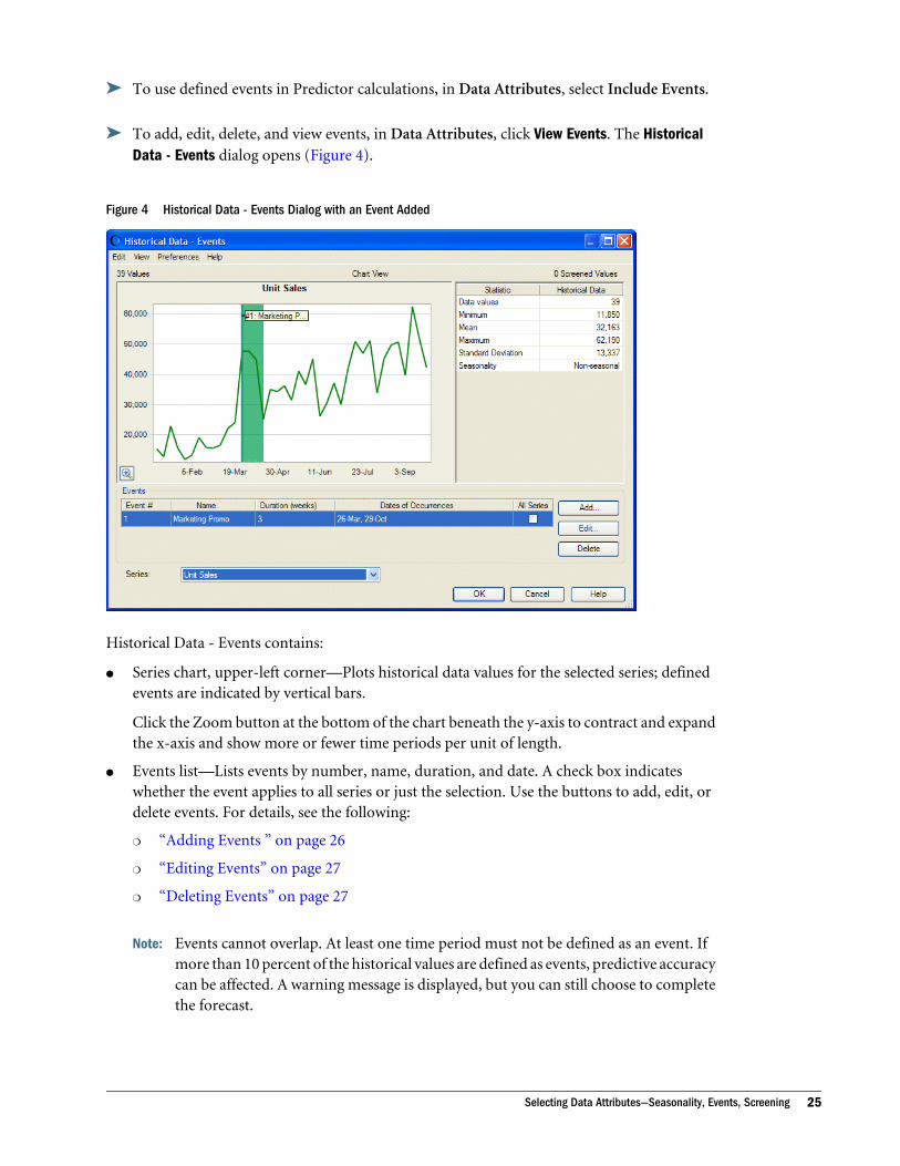
ä To add, edit, delete, and view events, in Data Attributes, click View Events. The HistoricalData - Events dialog opens (Figure 4).

Figure 4 Historical Data - Events Dialog with an Event Added

Historical Data - Events contains:

l Series chart, upper-left corner—Plots historical data values for the selected series; definedevents are indicated by vertical bars.

Click the Zoom button at the bottom of the chart beneath the y-axis to contract and expandthe x-axis and show more or fewer time periods per unit of length.

l Events list—Lists events by number, name, duration, and date. A check box indicateswhether the event applies to all series or just the selection. Use the buttons to add, edit, ordelete events. For details, see the following:

m “Adding Events ” on page 26

m “Editing Events” on page 27

m “Deleting Events” on page 27

Note: Events cannot overlap. At least one time period must not be defined as an event. Ifmore than 10 percent of the historical values are defined as events, predictive accuracycan be affected. A warning message is displayed, but you can still choose to completethe forecast.


l Series list, lower-left corner—Lists all the data series in the selected spreadsheet cell range.The currently selected series appears in the chart.

l Statistics, upper-right corner—Lists the following: number of historical data values,minimum value, mean value, maximum value, standard deviation of values, and the numberof time periods in a cycle, such as 12 months in a year.

l Menus that enable you to:

m Copy and print the chart (Edit menu)

m Switch among the historical data chart and a data table (View menu)

m Show and hide statistics (View menu)

m Set chart preferences (Preferences menu)

m Open Predictor help (Help menu)

Tip: You can view information for another data series by selecting it from the Series list.

After you define at least one event and check Include Events in Data Attributes, you can includeevents data in reports and extract events data. For instructions, see “Creating Reports” on page49 and “Extracting Results Data” on page 50.

Adding Events

ä To add an event:

1 In Data Attributes, click View Events.

2 In Historical Data – Events, click Add (Alt+a).

3 In the Add Event dialog, provide the following requested information:

l Name—A label to identify the event

l Apply to all series—When selected, applies the new event to all series, not just to thecurrent series

l Start date—The date the event or the first occurrence of the event began (“Setting EventDates” on page 27)

l Duration—The number of time periods that include a single occurrence of the effectsof the event; this number must be a whole number, not a decimal, greater than 0

l Repeats—Whether the event never repeats, repeats continuously at regular intervals, orrepeats at custom (irregular) intervals

To enter additional irregular intervals after the “Start date” entry (including intervalsin the future), select at custom intervals and follow the instructions in “Setting EventDates” on page 27.

If you select every, intervals are assumed to repeat in future predicted data as well as inpast historical data.


4 When settings are complete, click OK.

For a description of the Historical Data – Events dialog, see “Viewing and Managing Events” onpage 24.

Editing Events

ä To edit an event:


2 In Historical Data – Events, select an event and click Edit (Alt+t).

3 In Edit Event, edit the displayed information.

For a description of each edit box, see “Adding Events ” on page 26. For information on thestart date and custom date settings, see “Setting Event Dates” on page 27.


For a description of the Historical Data – Events dialog, see “Viewing and Managing Events” onpage 24.

Deleting Events

ä To delete an event:


2 In Historical Data – Events, select the event to delete and click Delete (Alt+d).

3 Select Yes to delete the event and No to keep it.


For a description of the Historical Data – Events dialog , see “Viewing and Managing Events”on page 24.

Setting Event Dates

Note: The following settings are in Add Event and Edit Event. See “Adding Events ” on page 26and “Editing Events” on page 27.

ä To set the start date of the first or only occurrence of an event, click Select (Alt+S) to displaya calendar. You can enter text in the Filter box to narrow the search. For example, if the time


period is months, enter M to display May and March for all years. An asterisk (*) is a“wildcard” symbol that matches any characters.

ä To set additional start dates for irregular occurrences after the first “Start date” entry:

1 Select at custom intervals, and then click Select (Alt+l) to display the Select Custom Dates dialog.

2 Use the arrow buttons to move dates from Available Dates to Selected Dates. These are start dates forother occurrences of that event that happen later than the start date entered in Add Events.

The duration is assumed to be the same as the duration entered in Add Events. You can useFilteras described for “Start date” earlier in this list.

3 To define start dates for event occurrences in the future, enter a number for Show Future Periods.

This setting is only for entering start dates. It is different from Periods to Forecast, shown inPredictor Results.

Viewing Screened DataYou can use the Predictor data screening features to:

l Fill in values that should exist in historical data but do not, such as data missing for onemonth in a five-year series (see “Selecting Data Attributes—Seasonality, Events, Screening”on page 19)

l Screen (exclude) outliers, values that differ significantly from the normal range of historicaldata

l Specify the statistical algorithms used to fill in or screen data (see “Setting ScreeningOptions” on page 28)

ä To examine the effects of filling in or screening data, and to change screening settings:

1 Click View Screened Data in the Data Attributes panel.

The Historical Data - Data Screening dialog opens. Any screened data values are highlightedin the chart.

2 Optional: Select Show screened data only to gray out unscreened data in the chart.

3 Optional: Click Screening Options to specify data filling and screening options. For details, see “SettingScreening Options” on page 28.

Setting Screening OptionsYou can choose from among several statistical methods to identify and adjust outliers and fillin missing values.

ä To select an outlier detection method:

1 In the Data Attributes panel, click View Screened Data.

The Historical Data - Data Screening dialog opens.


2 In Historical Data — Data Screening, click Screening Options.

The Data Screening Options dialog opens.

3 Select a detection method and enter an associated threshold value.

You can select outliers using the mean and standard deviation, the median and medianabsolute deviation (MAD), or the median and interquartile deviation (IQD). For adescription of each method, see “Outlier Detection Methods” on page 97. The default isMean and Standard Deviation with a standard deviation of 3.

ä To select a method for adjusting outliers and filling in missing values:

1 Display the Data Screening Options dialog as described in steps 1 and 2 above.

2 Select a method:

l Cubic spline interpolation calculates a smooth, continuous curve that passes througheach data point. It evaluates the entire data set.

l Neighbor interpolation examines values on each side of the value to be adjusted or filledin and calculates that value based on the mean or median of the specified neighbors.

For more information about each method, see “Outlier and Missing Value AdjustmentMethods” on page 99.

3 If you select Neighbor interpolation, indicate the number of neighbors to evaluate on each side of thetarget value and select a statistic.


Selecting a Forecasting MethodUse the Methods panel of the Predictor wizard to select a forecasting method.

ä To display Methods, click Next in Data Attributes or click Methods in the navigation pane ofthe Predictor wizard.

ä To select one or more forecasting methods:

1 Depending on the Data Attributes Seasonality setting and the nature of the data, select one or moreof the following:

l Non-seasonal Methods—Work best on data that do not show a pattern that repeatsregularly over a certain number of time periods, but can show a trend of decreasing orincreasing over time

l Seasonal Methods—Work best on data that show a pattern that repeats regularly overa certain number of time periods and can also show a trend of decreasing or increasingover time

l ARIMA—Useful in a variety of situations, particularly when there are many historicalvalues and very few outlier values

Selecting a Forecasting Method 29

l Multiple Linear Regression—Useful when independent variables affect another variableof interest

Note: Shortcut keys for selecting or clearing each method group are as follows: Ctrl+n, Non-seasonal Methods; Ctrl+s, Seasonal Methods; Ctrl+a, ARIMA; and Ctrl+m, MultipleLinear Regression.

2 Optional: Disable any individual method or override the default settings:

l For Non-seasonal Methods and Seasonal Methods, see “Using Classic Time-seriesForecasting Methods” on page 30 for help with selecting only a few methods or usingall of them (recommended). Note that you can double-click any method to change itsparameters and override the defaults.

l For ARIMA (autoregressive integrated moving average) methods), see “Using ARIMATime-series Forecasting Methods” on page 33.

l For Multiple Linear Regression, see “Using Multiple Linear Regression” on page 37.

3 When settings are complete, click Next to review and change forecasting options.

Using Classic Time-series Forecasting Methods

Note: This section describes non-seasonal and seasonal time-series forecasting methods that donot include Box-Jenkins ARIMA methods. For information on those methods, see “UsingARIMA Time-series Forecasting Methods” on page 33.

You can forecast historical data using many different time-series forecasting methods. Somemethods are designed to work best for certain types of data:

l Seasonal data (increasing or decreasing in a regularly recurring pattern over time; Figure 5,left side)

l Trend data (consistently increasing or decreasing over time; Figure 5, right side)

l Data with no trend or seasonality

Figure 5 Seasonal Data (Left) and Data with a Trend (Right)

In addition to these categories, there are two types of seasonal methods: additive andmultiplicative. Additive seasonality has a steady pattern amplitude, and multiplicative


seasonality has the pattern amplitude increasing or decreasing over time. Figure 6 illustratesthese different curves.

Figure 6 Different Seasonal Curves

For time-series forecasting, any of the classic time-series forecasting methods should work withdifferent amounts of success. However, each method has its own purpose, as described inTable 1 and the summary paragraphs that follow it. For more information about each classicmethod, see “Classic Non-seasonal Forecasting Methods” on page 83 and “Classic SeasonalForecasting Methods” on page 85.

Table 1 Choosing a Classic Time-series Forecasting Method

No Trend or Seasonality Trend Only, No Seasonality Seasonality Only, No Trend Both Trend and Seasonality

Single exponential smoothing Double exponential smoothing Seasonal additive Holt-Winters' additive

Single moving average Double moving average Seasonal multiplicative Holt-Winters' multiplicative

To summarize selection guidelines:

l Moving average methods—These methods help to smooth out short-term fluctuations andhighlight longer-term trends or cycles. They are used when the time series does not have atrend. When the time series has a trend, using the double moving average method computesa second moving average from the original moving average to track the trend better.

l Exponential smoothing methods—While the moving averages give equal weights toincluded values, single exponential smoothing assigns exponentially decreasing weights asthe observation get older, a more reasonable approach. When a time series has a trend,double exponential smoothing is useful and is computed by smoothing the series twice.


ä To determine whether you have trend or seasonal data, click View Seasonality on the InputData panel. For details, see “Viewing Historical Data by Seasonality” on page 20.

Tip: Viewing seasonality can help you decide which methods to select. However, selecting allthe classic time-series forecasting methods available for either Non-seasonal Methods orSeasonal Methods does not significantly slow down the calculations unless you areforecasting thousands of values at once, so you can consider trying them all (the default).

ä For forecasting method selection procedures, see “Selecting a Forecasting Method” on page29.

ä To manually set the parameters for any method, see “Setting Classic Time-series ForecastingMethod Parameters” on page 32, following.

Setting Classic Time-series Forecasting Method Parameters

Note: This section describes classic non-seasonal and seasonal time-series forecasting methodsand does not include Box-Jenkins ARIMA methods. For information on those methods,see “Using ARIMA Time-series Forecasting Methods” on page 33.

ä To manually set the parameters for any classic time-series forecasting method, overridingthe automatic calculation of parameters:

1 Double-click in the method area.

The method’s Parameters dialog opens.

2 Optional: Select Optimize to automatically optimize the parameters using error measures.

3 Optional: Select Lock Parameters to enter new parameter values in the parameter fields.

For more information on these parameters, see “Classic Non-seasonal Forecasting MethodParameters” on page 85 and “Classic Seasonal Forecasting Method Parameters” on page87.

4 Click OK.

Note: The user-defined settings remain for the current data selection until you reset them. ClickSet Default to restore default settings for future data selection.


Using ARIMA Time-series Forecasting Methods

Subtopics

l Selecting an ARIMA Model Selection Criterion

l Using ARIMA Custom Models

l Adding Custom ARIMA Models

l Editing Custom ARIMA Models

l Setting ARIMA Options

Autoregressive integrated moving average (ARIMA) forecasting methods were popularized byG. E. P. Box and G. M. Jenkins in the 1970s. These techniques, often called the Box-Jenkinsforecasting methodology, have the following steps:

1. Model identification and selection

2. Estimation of autoregressive (AR), integration or differencing (I), and moving average (MA)parameters

3. Model checking

ARIMA is a univariate process. Current values of a data series are correlated with past values inthe same series to produce the AR component, also known as p. Current values of a randomerror term are correlated with past values to produce the MA component, q. Mean and variancevalues of current and past data are assumed to be stationary, unchanged over time. If necessary,an I component (symbolized by d) is added to correct for a lack of stationarity throughdifferencing.

In a non-seasonal ARIMA(p,d,q) model, p indicates the number or order of AR terms, d indicatesthe number or order of differences, and q indicates the number or order of MA terms. The p,d, and q parameters are integers equal to or greater than 0.

Cyclical or seasonal data values are is indicated by a seasonal ARIMA model of the format

SARIMA(p,d,q)(P,D,Q)(t)

The second group of parameters in parentheses are the seasonal values. Seasonal ARIMA modelsconsider the number of time periods in a cycle as defined in the Historical Data – Seasonalitydialog (Figure 2 on page 21). For a year, the number of time periods (t) is 12.

Note: In the Predictor user interface, seasonal ARIMA models do not include the (t) component,although it is still used in calculations. See the Bibliography for references that describethis methodology in more detail.

Crystal Ball ARIMA models do not fit to constant datasets or datasets that can betransformed to constant datasets by non-seasonal or seasonal differencing. Because ofthat feature, all constant series, or series with absolute regularity such as data representinga straight line or a saw-tooth plot, do not return an ARIMA model fit.


ä To use ARIMA methods:

1 In the Predictor wizard Methods panel, select ARIMA.

2 In the Autoregressive Integrated Moving Average (ARIMA) Details panel, select Automatic (thedefault) or Custom models.

Note: Unless you are thoroughly acquainted with ARIMA methodology and intend toconstruct or use existing custom ARIMA models, select Automatic.

3 Optional: If you selected Automatic, select a model selection criterion, Minimize informationcriterion (the default) or Minimize selected error measure. The default generally provides a betterARIMA estimate. Minimizing the error measure selected elsewhere for Predictor forecasting can resultin overfitting.

4 Optional: Click Select Information Criterion (Alt+e) to indicate which information criterion to use. Fordetails, see “Selecting an ARIMA Model Selection Criterion” on page 34. Unless you have good reasonto select another, BIC (the default) is usually appropriate.

5 Optional: Select Perform extended model search to compare more models to the historical data. Resultsmay be somewhat more accurate, but the analysis can take noticeably more time.

6 Optional: If you selected Custom models in step 2, build a list of models to use. For instructions, see“Using ARIMA Custom Models” on page 35.

7 Optional: Click ARIMA Options (Alt+o) to indicate whether to include a constant in the ARIMA equationand whether to perform a Box-Cox transformation. The default, AutoSelect or None, is usuallyappropriate for both options. For more information, see “Setting ARIMA Options” on page 36.

Note: If Automatic is selected, any displayed models are fitted to each series. Custom seasonalmodels are not fitted to non-seasonal series, but non-seasonal models will be fitted toseasonal series.

If Custom models is selected, models apply only to the currently selected Predictor seriesand must be defined for each series separately.

Selecting an ARIMA Model Selection Criterion

ä To select an ARIMA model selection criterion:


2 In the Autoregressive Integrated Moving Average (ARIMA) Details panel, select Automatic (thedefault).

3 Select Minimize Information Criterion, and then click Select Information Criterion (Alt+e).

4 In the Select Information Criterion dialog, select a setting:

l Bayesian Information Criterion (BIC)

l Akaike's Information Criterion (AIC)

l Corrected AIC (AICc)


Note: See the Bibliography for references that discuss the differences among these criteria.The three criteria differ in the way that they penalize overfitting. The differences aresmall, and the chosen criterion typically does not lead to a change in the ARIMAmodel selected as the best fit.

Using ARIMA Custom ModelsWhile automatic selection of an ARIMA model should be completely adequate, if results aredifferent from what you expect and you are familiar with ARIMA methodology and modelconstruction, you can create and edit ARIMA models in Predictor.

ä To use custom models for ARIMA forecasting:


2 In the Autoregressive Integrated Moving Average (ARIMA) Details panel, select Custom models.

3 Click a button to add, edit, or remove a model:

l Add (Alt+d), enables you to create a new model, as described in “Adding Custom ARIMAModels” on page 35.

l Edit (Alt+e), enables you to modify the selected model, as described in “Editing CustomARIMA Models” on page 36.

l Remove (Alt+v), permanently deletes the selected model.

Note: Displayed models are fitted to each series. Custom seasonal models are not fitted to non-seasonal series, but non-seasonal models are fitted to seasonal series.

Adding Custom ARIMA Models

ä To add a custom model for ARIMA forecasting:

1 Follow steps 1 and 2 in “Using ARIMA Custom Models” on page 35.

2 Click Add (Alt+d).

3 In the Add ARIMA Model dialog, indicate the orders for each parameter of the non-seasonal and,optionally, seasonal model, and then click OK.

Follow these rules for entering model orders:

l Non-seasonal component orders can be 0 to 10. Seasonal component orders can be 0to 2.

l Orders must be integers.

l At least one parameter of the non-seasonal or seasonal model component must be non-zero.

l As with standard ARIMA notation, the p portion of the model definition goes in the ARfield, the q portion in the MA field, and the d portion in the I field.


l The time-period portion of a seasonal model is taken from the existing Predictorinformation for that series but is not included in the Custom models list.

4 When the definition is complete, click OK.

The new model is displayed in the Custom models list. Seasonal models are preceded by S—SARIMA(2,0,3)(1,0,2), for example.

Editing Custom ARIMA Models

ä To edit a custom model for ARIMA forecasting:

1 Follow steps 1 and 2 in “Using ARIMA Custom Models” on page 35.

2 Click Edit (Alt+e).

3 In the Edit ARIMA Model dialog, indicate the orders for each part of the non-seasonal and, optionally,seasonal model, and then click OK.

For model rules, see “Adding Custom ARIMA Models” on page 35.

4 When the definition is complete, click OK.

Setting ARIMA OptionsARIMA equations can include a constant that represents the intercept if the AR portion of amodel is not 0; otherwise, it represents the mean of the series. You can set ARIMA options toindicate whether to include the constant in ARIMA equations. The ARIMA options can also beused to provide variance stationarity in data using the Box-Cox transformation. If you choose

to apply the Box-Cox transformation, you can select from among several lambda (λ) options.For more information, see the Oracle Crystal Ball Statistical Guide.

The ARIMA options settings apply to both automatic and custom-model ARIMA forecasts.AutoSelect is the default for the constant option; None is the default for the Box-Cox option.

ä To set ARIMA options:


2 In the Autoregressive Integrated Moving Average (ARIMA) Details panel, click ARIMA Options (Alt+o).

3 In the ARIMA Options dialog, indicate whether to:

l Include the constant in ARIMA equations by selecting AutoSelect (the default), Always,or Never

l Perform no Box-Cox transformation (None); or perform a Box-Cox transformationwith an Optimized value for lambda or a Square root, Logarithmic, or Custom lambda value(between –5 and +5, inclusive)


Note: If you select AutoSelect for constant inclusion, Predictor includes a constant in theARIMA equation only when the model does not include a non-seasonal or seasonaldifference term.

Using Multiple Linear RegressionIf you know that some independent variables affect another variable of interest (the dependentvariable), use multiple linear regression as the forecasting method for that variable. For example,summer temperatures affect electricity usage because, as it gets hotter, more people run their airconditioning. This means that electricity usage (the dependent variable) is dependent on thetemperature (an independent variable).

Predictor follows this process to forecast a dependent variable with regression:

1. Creates an equation that defines the mathematical relationship between the independentvariables and a dependent variable. This is the regression equation.

2. Forecasts each independent variable by running all the selected time-series forecastingmethods for each one and using the best method for each.

3. Calculates the regression equation with the forecasted independent variable values to createthe forecast for the dependent variable.

ä To use multiple linear regression:

1 On the Predictor wizard Methods panel, select Multiple Linear Regression.

2 In the Regression Variables dialog, select dependent and independent variables. For instructions, see“Selecting Regression Variables” on page 38.

3 Select the regression method to use: Standard, Forward stepwise, or Iterative stepwise. Fordescriptions, see “Regression Methods” on page 93.

4 If you selected a stepwise regression, you can select associated settings.

For instructions, see “Setting Stepwise Regression Options” on page 38.

5 Select or clear the remaining settings:

l Include constant in regression equation—Includes the y-intercept constant in theregression equation; if not selected, the regression equation passes through the origin.This setting is selected by default.

l Run only regression method for dependent variables—If selected, forecasting methodsother than regression are not run on dependent variables. By default, this setting is notselected and all the forecasting methods run on these variables along with linearregression.

l Calculate variance inflation factor (VIF) for independent variables—Calculates theVariance Inflation Factor (VIF) of each independent variable included in the regressionequation, where VIF is a measure of the strength of multicollinearity (amount ofcorrelation) between the independent variables. Calculating the VIF requires additionaltime. By default, this setting is not selected.


Note: For rules concerning minimum number of data points required for multiple linearregression, see “Creating Spreadsheets with Historical Data” on page 12.

Selecting Regression VariablesThe Regression Variables dialog opens when you select Multiple Linear Regression in theMethods panel of the Predictor wizard.

ä To select dependent and independent variables for regression analysis:

1 In the Regression Variables dialog, move the dependent variables into the Dependent variables(Y's) list:

a. Select the name of a dependent variable in the Independent variables (X's) list.

You can have more than one dependent variable. Predictor forecasts them all, one at atime, as functions of all the same independent variables.

b. Click between the lists.

The variable moves to Dependent variables (Y's).

2 Confirm that all variables are included in the appropriate list.

3 To lag independent variable data by a number of time periods:

a. Select a variable in Independent variables (X's).

b. Enter the number of time periods to lag the variable in the Lag text box below the list.

c. Repeat for any other independent variables you want to lag.

4 Clear the check box for any variables you do not want to include in the regression.

5 Click OK.

The Methods panel is displayed again (see “Using Multiple Linear Regression” on page 26).

Setting Stepwise Regression OptionsThe Stepwise Options dialog opens when you select one of the stepwise regression methods inthe Methods panel of the Predictor wizard.

ä To set appropriate stepwise method options:

1 In the Stepwise Options dialog, select R-Squared and Partial F-Test settings.

Fields, settings, and buttons in the Stepwise Options dialog:

l R-Squared—Stops the stepwise regression if the difference between a specified statistic(either R-Squared or Adjusted R-Squared) for the previous and new regression solutionis below a threshold value. When this happens, Predictor does not use the new regressionsolution. By default, this stopping criterion is selected and uses R-Squared as the statistic.If this setting and the Partial F-Test Significance are selected, the stepwise regressionstops when it reaches either criterion’s threshold value.


l Threshold—Sets the minimum increment required between the R-Squared or AdjustedR-Squared of the last step and the R-Squared or Adjusted R-Squared of the new step tocontinue with the stepwise regression. The default is 0.001.

l Partial F-Test Significance—Stops the stepwise regression if the probability of the Fstatistic for a new solution is above a maximum value. By default, this stopping criterionis not selected. If this setting and the R-Squared setting are selected, the stepwiseregression stops when it reaches either criterion’s threshold value.

l Probability to add—Sets the maximum probability of the correlation (partial F statistic)of the independent variable required to add the variable to the regression equation. Thedefault is 0.05. When dealing with statistical tests, smaller probabilities indicate moresignificance.

l Probability to remove—Sets the minimum probability of the correlation (partial Fstatistic) of the independent variable required to remove the variable from the regressionequation. The default is 0.05. This setting is only available with iterative stepwiseregression. The Probability to remove setting must be at least 0.05 higher than theProbability to add setting.

2 Click OK.

The Methods panel is displayed again (see “Using Multiple Linear Regression” on page 37).

Setting Forecast OptionsUse the Options panel of the Predictor wizard to select an error measure and a forecastingtechnique. To display Options, click Next in Methods or click Options in the navigation paneof the Predictor wizard.

The following topics describe how to set the forecast options:

l “Selecting Error Measures” on page 39

l “Selecting Forecasting Techniques” on page 40

When all Options settings are complete, click Run to run the forecast and produce results. Formore information, see “Starting Predictor and Running a Forecast” on page 13.

Selecting Error MeasuresPredictor uses one of three error measures to determine which time-series forecasting methodworks best. When determining the best method, Predictor calculates the selected error measurewhen fitting each method to the historical data. The method with the lowest error measure isconsidered best, and the rest of the methods are ranked accordingly.

By default, Predictor uses RMSE to select the best method.

ä To change which error measure Predictor uses:

1 On the Options panel, select the error measure you want Predictor to use to determine the best method:

Setting Forecast Options 39

l RMSE - Root Mean Squared Error

l MAD - Mean Absolute Deviation

l MAPE - Mean Absolute Percentage Error

For more information on these error measures, see “Time-series Forecasting AccuracyMeasures” on page 88.

2 Follow the instructions in “Selecting Forecasting Techniques” on page 40 to complete the Optionssettings and prepare to run the forecasts.

Selecting Forecasting TechniquesPredictor uses one of four forecasting techniques for time-series forecasting: Standard, Simplelead, Weighted lead, and Holdout. By default, Predictor uses Standard forecasting to select thebest method.

ä To change which forecasting technique Predictor uses:

1 On the Options panel, select the forecasting technique to use for time-series:

l Standard forecasting—Error measure between the fit values and the historical data forthe same period; the default

l Simple lead—Error measure between the historical data and the fit offset by a specifiednumber of periods (lead)

l Weighted lead—Average error measure between the historical data and the fit offset by0, 1, 2, etc. periods, up to the specified number of periods (weighted lead)

l Holdout—Error measure between a set of excluded data and the forecasting values.Predictor does not use the excluded data to calculate the forecasting parameters

For more information about each technique, see “Time-series Forecasting Techniques”on page 90.

2 If you select Simple lead, Weighted lead, or Holdout, enter the appropriate lead or holdout in the box.

3 If all settings in the Predictor wizard are complete, click Run to run the forecast and produce results.


4Analyzing Predictor Results

In This Chapter

Understanding the Predictor Results Window ... . . . . . . . . . . . . . . . . . . . . . . . . . . . . . . . . . . . . . . . . . . . . . . . . . . . . . . . .41

Selecting How to Display and Analyze Results .. . . . . . . . . . . . . . . . . . . . . . . . . . . . . . . . . . . . . . . . . . . . . . . . . . . . . . . . .44

Adjusting Forecasted Data ... . . . . . . . . . . . . . . . . . . . . . . . . . . . . . . . . . . . . . . . . . . . . . . . . . . . . . . . . . . . . . . . . . . . . . . . . . . . . .44

Pasting Predictor Forecasts .. . . . . . . . . . . . . . . . . . . . . . . . . . . . . . . . . . . . . . . . . . . . . . . . . . . . . . . . . . . . . . . . . . . . . . . . . . . . . .46

Viewing Charts.. . . . . . . . . . . . . . . . . . . . . . . . . . . . . . . . . . . . . . . . . . . . . . . . . . . . . . . . . . . . . . . . . . . . . . . . . . . . . . . . . . . . . . . . . . . . .47

Creating Reports .. . . . . . . . . . . . . . . . . . . . . . . . . . . . . . . . . . . . . . . . . . . . . . . . . . . . . . . . . . . . . . . . . . . . . . . . . . . . . . . . . . . . . . . . . .49

Extracting Results Data ... . . . . . . . . . . . . . . . . . . . . . . . . . . . . . . . . . . . . . . . . . . . . . . . . . . . . . . . . . . . . . . . . . . . . . . . . . . . . . . . . .50

Understanding the Predictor Results Window

Subtopics

l Entering the Number of Time Periods to Forecast

l Selecting a Confidence Interval

The Predictor Results window (Figure 7) is similar to the Historical Data dialog described in“Viewing Historical Data by Seasonality” on page 20.

Understanding the Predictor Results Window 41

Figure 7 Predictor Results Window with Shampoo Sales Results Including Events

l The Series group determines which data series is displayed. If you forecasted results for morethan one series, look at all results by selecting each series in the Series list.

l By default, the displayed information is calculated using the forecasting method listed asBEST. You can view a different method for each series if you want. The methods are orderedfrom best to worst.

You can override the best method to calculate results using the new “best” method. Thischange only affects the current series. The other series remain unchanged unless you selectone and override its method also.

If you change the method selection for a given series and then select another series and comeback to the original series, it is the best method for the original series that is selected (notany non-best selection that might have been active when the series was changed). To alwaysview a particular method when a particular series is selected, the best method should beoverriden for that series.

l The chart of series data values includes historical and predicted, or forecasted, data. Plots ofraw data values and fitted values are displayed for historical data. Forecasted data values areenclosed by lines that show the upper and lower confidence intervals (described in “Selectinga Confidence Interval” on page 43). You can use Ctrl+p to display and hide confidenceinterval lines on the chart.

l In the case of a dependent regression variable, the forecasted values are a function of thebest forecast methods (or overridden best forecasting methods) of the independentvariables.

l If you have defined at least one event and selected Include events in the Data Attributes panel,a shaded vertical bar displays through historical and predicted data defined as events. You

42 Analyzing Predictor Results

can select Preferences, and then Highlight Events to hide these bars and display them again(see Figure 7 on page 42).

Note: You can also select Highlight Seasonality and Highlight Screened Data to show or hideindications of seasonal cycles or filtered data if those features if they are selected inthe Predictor wizard and included within displayed data.

l In the upper-right is a table of statistics for the raw historical data. For more informationabout these statistics, see “Historical Data Statistics” on page 96.

l Below the historical statistics are error statistics for the forecasted data values. These statisticsare described in “Time-series Forecasting Accuracy Measures” on page 88.

l At the bottom of the statistics table are parameter values for the currently selected forecastingmethod. See “Classic Non-seasonal Forecasting Method Parameters” on page 85 and“Classic Seasonal Forecasting Method Parameters” on page 87.

l The Forecasts group is used to change the number of time periods to forecast and to selectconfidence interval boundaries. See “Entering the Number of Time Periods to Forecast” onpage 43 and “Selecting a Confidence Interval” on page 43.

You can also use the Adjust and Paste buttons to adjust missing values and outliers (extremevalues) and paste forecasted values into the Predictor model (“Adjusting Forecasted Data”on page 44 and “Pasting Predictor Forecasts” on page 46).

l You can right-click within the Predictor Results window to display a menu with relatedcommands.

For additional information, see “Selecting How to Display and Analyze Results” on page 44.

Entering the Number of Time Periods to ForecastAfter Predictor determines the method that best fits the historical data, it can use that samemethod to forecast future values. You need to decide how many time periods to forecast.

Consider these factors:

l The first few values are fairly reliable. Forecast only as many values as you need.

l The farther out you try to forecast, the less reliable the forecasted values are. The confidenceinterval of any forecast grows to reflect this decrease in reliability.

ä To indicate how many time periods to forecast, enter the number in Periods to forecast inthe lower-right corner of the Predictor Results window.

Selecting a Confidence IntervalThe confidence interval defines the range above and below a forecasted value where the valuehas some probability of occurring. For example, a confidence interval of 10% and 90% gives twopoints for each forecasted value. The lower point represents the 10th percentile. The higher point

Understanding the Predictor Results Window 43

represents the 90th percentile. There is an 80% chance the predicted value will fall within thisrange. The farther out the forecast is, the larger this range is.

ä To select a confidence interval, select from the Confidence interval list in the lower rightcorner of the Predictor Results window or choose Custom to enter the desired confidenceinterval in the Custom Confidence Interval dialog.

Selecting How to Display and Analyze ResultsYou can use Predictor results in several ways:

l Adjust the forecasted data, including rounding it

l Paste the forecasted data anywhere on the worksheet or into a new worksheet

l View, copy, and print charts that can show historical data, fitted values, forecasted data, andassociated confidence intervals

l Generate a report summarizing the findings

l Create an interactive table of all the historical data, fitted values, forecasted data, andconfidence intervals

l Create an interactive table of some or all the method information for each forecast, includingthe errors, parameters, and statistics for each method tried

For instructions:

l “Adjusting Forecasted Data” on page 44

l “Pasting Predictor Forecasts” on page 46

l “Viewing Charts” on page 47

l “Creating Reports” on page 49

l “Extracting Results Data” on page 50

Adjusting Forecasted DataAfter you run a Predictor forecast, you can adjust the forecasted data to customize it for yourparticular situation. For example, you could add 50 to each forecasted value, or you could roundeach value to the nearest hundreds. Adjustments are applied to all methods for that series.

ä To adjust forecasted data:

1 Run a Predictor forecast and display the Predictor Results window.

2 Click Adjust.

3 In the Adjust Forecast for Series dialog, change any or all settings in the listed order:

l 1. Percentile of forecast range—See the note below for an explanation; select Custom toenter a percentile into the Custom Percentile dialog (Default = Median)


l 2. Adjust values by—Increases or decreases each value by the specified amount (Default= 0.00)

l 3. Round values to—Rounds values to the specified numeric place; for example Integerrounds to the nearest number in units place (Default = No rounding; select Custom tospecify a decimal place as described in “Custom Rounding” on page 45)

l 4. Restrict values to range—Limits adjusted values to the specified range (Default = –Infinity to Infinity)

Note: When a time-series forecast is pasted into a model as a Crystal Ball assumption, eachforecast value is assumed to be the median, or 50th percentile, of a normal distributionassumption. The percentile adjustment is ignored in this case.

4 Optional: Click Apply to All Series to apply the settings to all data series, except for dependent variablesin a regression analysis.

5 Optional: Click Defaults to restore all the default settings.

6 When setting changes are complete, click OK.

Custom RoundingSeveral rounding settings are available in the Adjust Forecast for Series dialog; you can also specifycustom rounding levels.

ä To specify a custom rounding level:

1 In the Adjust Forecast for Series dialog, select Custom for 3. Round values to.

2 In the Custom Rounding dialog, specify a rounding level:

l 0 = first place to the left of the decimal (units place)

l 1 = second place to the left of the decimal (tens)

l 2 = third place to the left of the decimal (hundreds)

l 3 = fourth place to the left of the decimal (thousands)

l –1 = first place to the right of the decimal (tenths)

l –2 = second place to the right of the decimal (hundredths)

l –3 = third place to the right of the decimal (thousandths)

Increased positive and negative values continue this pattern. The default is 0. The validrange of entries is –15 to 15, inclusive.

Adjusting Forecasted Data 45

Pasting Predictor Forecasts

Subtopics

l Time-series Forecast Method Results

l Multiple Linear Regression Results

ä To paste forecasted values into a Microsoft Excel worksheet:

1 In the Predictor Results window, set Periods to forecast to the number of time periods to paste intothe worksheet.

2 Click Paste.

3 Select from among these settings in the Paste Forecasts to Spreadsheet dialog:

l Location:

m At end of historical data—Pastes forecasted data after the historical data

m Starting at cell—Pastes data in the specified cell and following cells; select a rangeto paste multiple data series

Note: Data is pasted below or to the right of the specified cell, depending on theOrientation selection.

l Options:

m Include date series—Pastes date labels next to forecasted values

m Paste forecasts as Crystal Ball assumptions—Creates pasted cells as Crystal Ballassumptions defined as normal distributions with a mean that is the forecasted valueand a standard deviation that is based on the RMSE of the fitted data

Note: Predictor does not create assumptions if the variation in the data is zero orapproaches infinity.

l Formatting:

m AutoFormat—Formats data to match the numerical formatting of the data seriesand highlights forecasts in bold

4 Click OK.

The results paste at the specified location. They are forecasted using the currently selected BESTmethod shown in the Predictor Results window.

Although Predictor tried all the methods you selected in the Method Gallery, it generates thepasted values using the best method, unless you overrode the best method, which is then usedinstead.

Note: Of the eight classic time-series forecasting methods, two result in flat lines: single movingaverage and single exponential smoothing. The forecasted values for these are all the same.This result is not an error. It is the best possible forecast for volatile or patternless data.


When you paste regression results, the independent variable forecast values are pasted as simplevalue cells. The dependent variable forecasted values are created as formula cells with theregression equation as the formula. The regression equation coefficients appear below the pastedvalues.

Time-series Forecast Method ResultsFor data series forecasted using time-series methods, Predictor creates the assumptions asnormal distributions with a mean equal to the forecasted value in the cell and a standarddeviation calculated using the RMSE.

Multiple Linear Regression ResultsFor multiple linear regression, Predictor creates assumptions for the independent variableforecast values only. This is because the independent variable values are simple value cells, butthe dependent variable values are formula cells that are a function of the independent variables.

To see the variability of the dependent variable, select the pasted formula cells and define themas Crystal Ball forecast cells. (To do this, select Define, and then Define Forecast.) More likely,you will want to create one formula cell that represents the sum of the data in the dependentvariable cells and define that formula cell as a Crystal Ball forecast.

Viewing Charts

Subtopics

l Customizing Charts

l Copying and Printing Charts

By default, the Predictor Results window contains a chart of historical and forecasted values inthe upper left.

ä To control the chart view, use these settings:

l Periods to forecast— Determines the number of forecasted values that appear in the chart

l Confidence interval—Indicates which confidence interval to calculate and plot

l Series—Selects the data series to display in the chart

l Method—Selects the method to use for calculating forecasted values

l View menu—View, Table changes the chart display to a table; View, Chart changes it back; andView, Show Statistics hides and displays the statistics tables to enlarge the chart

Note: If Include events is selected in the Data Attributes panel of the Predictor wizard, andat least one event is defined, Table View includes an Event column with the name andnumber of each event defined for the selected series.

Viewing Charts 47

l Preferences menu—Preferences, Chart displays the Chart Preferences dialog (see“Customizing Charts” on page 48, following); Preferences, Show All Error Measures hidesand shows error measures that are not selected in the Options panel of the Predictor wizard;Preferences, Highlight Seasonality graphically emphasizes seasonal data cycles if present;Preferences, Highlight Screened Data emphasizes filled-in or adjusted-outlier data if theseare present and you selected at least one of the Data Screeningsettings in the Data Attributespanel; and Preferences, Highlight Events emphasizes data defined as events if you have definedat least one event and selected Include events in the Data Attributes panel.

Chart Notes

l As shown in the chart legend, the green line represents the historical data, the blue linesrepresent fitted and forecasted values, and the red dotted lines above and below theforecasted values represent the upper and lower confidence interval. A gap between thehistorical and forecasted values delineates the past and future values.

l Of the eight classic time-series forecasting methods, four result in straight lines: singlemoving average, single exponential smoothing, double moving average, and doubleexponential smoothing. Only the seasonal methods and multiple linear regression result incurves that approximate repeated data patterns.

Customizing ChartsYou can customize Predictor charts in many ways:

l Change the colors of lines and line types in the chart

l Display and hide the grid lines and legend

l Show the chart in perspective for a 3D effect

l Make the chart lines transparent

ä To customize Predictor charts:

1 In the Predictor Results window, select Preferences, and then Chart Preferences.

2 In the Chart Preferences dialog, review the Show Series settings:

l Clear the check box for any series that you do not want to include.

l Make desired line color or line type changes.

3 Optional: Review the Options settings:

l Change the Gridlines setting to display horizontal or vertical gridlines.

l Change the Legend setting to display or hide the legend and change its position in thechart.

4 Optional: Review the Effects settings:

l Select the 3D chart setting to add three-dimensional perspective.

l Select the Transparency setting to make the chart lines transparent, according to thenumber in the percent box.


5 Click OK to return to the Predictor Results window.

Copying and Printing Charts

ä To copy and print charts:

1 In the Predictor Results window, select Edit.

2 Perform an action:

l Select Copy Chart to copy the chart to the Windows clipboard.

l Select Page Setup, Print Preview, or Print to perform those printing tasks withWindows-standard dialogs.

Creating Reports

ä To create a report of Predictor data for each series:


If it is not visible, click Predictor Results in the Windows task bar. (It may be located in theMicrosoft Office Excel group.)

2 Confirm that the following settings are complete and correct:

l Periods to forecast— Determines the number of forecasted values that are displayed


l Series—Selects the data series to display

l Method—Selects the forecasting method used to calculate forecasted values

See “Viewing Charts” on page 47.

3 In the Predictor Results menu bar, select Analyze, and then Create Report.

4 In the Create Report Preferences dialog, select a report type:

l Predictor includes only Predictor data.

l Full and Custom can include all other available data as well as Predictor data. Forinformation about Full and Custom reports, click Help.

Note: If Include events is selected in the Data Attributes panel of the Predictor wizard, andat least one event is defined, the Events table is part of the Statistics section of theSeries report. For custom reports, events data display is controlled by the Statisticscheck box in the Predictor Series settings of the Custom Report dialog.

5 Optional: Click Options to specify a location and formatting for the report. For an explanation of eachsetting, click Help.

6 Click OK.

Creating Reports 49

By default, the report is created in a separate workbook. See Figure 17 on page 65.

Extracting Results DataYou can extract results and methods data from the current Predictor forecasting run.

ä To extract Predictor results:



2 Confirm that the following settings are complete and correct:

l Periods to forecast—Determines the number of forecasted values that are displayed


l Series—Selects the data series to display

l Method—Selects the forecasting method used to calculate forecasted values

See “Viewing Charts” on page 47.

3 In the Predictor Results menu bar, select Analyze, and then Extract Data.

4 In the Extract Data Preferences dialog, select the Predictor Data tab, if it is not already visible, andselect Results Table, Methods Table, or both:

l Results Table shows fit and residual values for historical data, forecast and confidenceinterval values for the forecasted values (where residuals are the difference between thefit value and the historical data value), and events data (if selected).

Note: If Include events is selected in the Data Attributes panel of the Predictor wizard,and at least one event is defined, an additional Event column in the table ofextracted data shows the event numbers defined for each series. Rows with eventsare also color coded. If the data has seasonality, seasonal differences are indicatedwith lighter colored rows. Screened data rows can also be highlighted. To changehighlighting of these special types of data, select the Results Window and thenselect Preferences and any of the Highlight commands.

l Methods Table shows error measures, parameters, ranking, and statistics for eachselected fit method.

5 In the Results Table Details group, select the data types to include.

Leave the defaults selected to extract all available data.

6 Click Options and confirm that the desired location and formatting settings are selected.

For details, select Help.

7 Click OK.


Depending on the Options settings, two tabs are displayed in the existing workbook or anew workbook. The tabs are Results Table and Methods Table. Each tab contains aninteractive Microsoft Excel PivotTable with the selected data. See “Analyzing and UsingExtracted Results” on page 39.

Analyzing and Using Extracted ResultsYou can use extracted data as input for spreadsheet analysis or you can copy it into otherapplications. For an example of how to use the Results and Methods tables, see “Working withData in Interactive Tables” on page 66. These are Microsoft Excel PivotTables, described inMicrosoft documentation and help.

Results Table

Even though Predictor tried all the methods you selected in the Method Gallery, it generates theResults table using the best method, unless you overrode the best method, in which case, theprogram generates the result values using the overriding method.

Methods Table

The Methods table reports all the parameters and statistics for the methods you selected in theMethods panel. The method used to generate the forecasted values, either the best method orthe overriding method, is highlighted in bold text. The method is likely to be different for eachforecasted series.

To compare the quality of the results of different time-series forecasting methods, check theerrors: RMSE, MAD, and MAPE. For all of these, the smaller the better. If you compare theRMSE of one method to the RMSE of another method, the smaller one should be ranked better.However, you cannot compare the RMSE of one method to the MAD or MAPE of anothermethod. See “Time-series Forecasting Accuracy Measures” on page 88.

To compare the quality of a regression, look for the following values:

Table 2 Evaluating Regression Quality

Statistic Range Ideal Value Ideal Value Interpretation

R2 or Adjusted R2 0 to 1 Close to 1 The linear regression accounts for almost all the variability in the dependent data.

F probability 0 to 1 Less than 0.05 The quality of the overall regression (dependency of the dependent variable onthe independent variables) is good.

t probability 0 to 1 Less than 0.05 The quality of the coefficient of the regression equation is good.

Durbin-Watson 0 to 4 2 No autocorrelation (at lag 1) exists.

Theil’s U Greater than 0 Less than 1 The quality of the results is better than guessing.

See Appendix C, “Important Predictor Concepts,” and the Oracle Crystal Ball Statistical Guide.

Extracting Results Data 51


APredictor Tutorials

In This Appendix

About Predictor Tutorials .. . . . . . . . . . . . . . . . . . . . . . . . . . . . . . . . . . . . . . . . . . . . . . . . . . . . . . . . . . . . . . . . . . . . . . . . . . . . . . . . .53

Tutorial 1—Shampoo Sales ... . . . . . . . . . . . . . . . . . . . . . . . . . . . . . . . . . . . . . . . . . . . . . . . . . . . . . . . . . . . . . . . . . . . . . . . . . . . .53

Tutorial 2—Toledo Gas ... . . . . . . . . . . . . . . . . . . . . . . . . . . . . . . . . . . . . . . . . . . . . . . . . . . . . . . . . . . . . . . . . . . . . . . . . . . . . . . . . . .57

About Predictor TutorialsThis chapter contains:

l “Tutorial 1—Shampoo Sales” on page 53, a basic tutorial that shows how Predictor works

l “Tutorial 2—Toledo Gas” on page 57, an advanced tutorial that uses multiple linearregression for forecasting

For less detailed examples, see Appendix B, “Predictor Examples.”

Tutorial 1—Shampoo SalesThe easiest way to understand what Predictor does is to apply it to a simple example. In thisexample, you are sales manager for Tropical Cosmetics Co. The company’s latest product,shampoo with tropical ingredients, has been in the marketplace for almost a year. The vicepresident of marketing wants you to forecast the rest of the year’s shampoo sales and decidewhether to recommend investing in advertising or enhancements for this product.

You have the weekly sales numbers for the last nine months.

ä To begin the tutorial:

1 Start Crystal Ball, which automatically starts Microsoft Excel.

2 Select Help, then Crystal Ball, and then Examples Guide.

Note: In Microsoft Excel 2007 or later, select Resources in the Help group, and then selectExamples Guide.

3 In the Model Name list, click Shampoo Sales.

The Shampoo Sales spreadsheet opens (Figure 8).

About Predictor Tutorials 53

Figure 8 Shampoo Sales Spreadsheet

In this spreadsheet, column A contains dates from January 1, 2010 until September 24, 2010and column B contains Tropical shampoo sales data. You need to forecast sales through theend of the year, December 31, 2010.

4 Select cell B4, if it is not already selected.

Select any one cell in the data range, headers, or date range, and Predictor selects all the filledadjacent cells.


This command is available only if no simulation is running and the last run was reset. Ifnecessary, wait for a simulation to stop or reset the last simulation.

The Predictor wizard opens. If this is the first time you started Predictor, the Welcome panelis displayed. Otherwise, Input Data is displayed.

6 If Welcome opens, click Next to display Input Data.

When you select any one cell in the data range before you start the wizard, Predictordetermines:

l The data series (in this case, A3:B42)

l Whether the data values are in columns or rows

l Whether headers display at the beginning of the data

l Whether the first column or row contains dates or time periods

7 Confirm that cell range $A$3:$B$42 is selected and click Next.

The Data Attributes panel opens.

8 Confirm these settings and correct them if necessary:

l Data is in weeks.

54 Predictor Tutorials

l AutoDetect is selected to determine whether data has seasonality.

l In the Events group, Include events is selected.

l In the Data Screening group, Fill-in missing values is selected.

9 Click Next to open the Methods panel.

10 Leave the defaults selected and click Next to open the Options panel.

11 In Options, confirm that the defaults (RMSE and Standard forecasting) are selected, and then clickRun.

The Predictor Results window opens.

12 Set Periods to forecast to 14 and review window contents (Figure 9).

Figure 9 Predictor Results Window for the Shampoo Sales Spreadsheet Model

The Predictor Results window contains the following:

l A chart of historical and forecasted values; forecasted values appear as a dark blue lineextending to the right of the historical data (green) and the fitted values (blue). Aboveand below the forecasted values is the confidence interval (a red dotted line), showingthe 2.5th and 97.5th percentiles of the forecasted values. This is called a 95% confidenceinterval.

l A marketing event was defined for this model, indicated by vertical bars and labels.Because the historical data showed an increase during the event, the predicted data alsoshows an increase when the event is scheduled to repeat.

Tutorial 1—Shampoo Sales 55

Note: You can select Preferences, and then Highlight Events to hide the event labels andbars.

l A Series list of all data series selected for forecasting; onscreen information pertains tothe selected series

l A Method list of all the methods Predictor tried, in order from the best-fitting methodto the worst-fitting method. Predictor calculates the forecasted values from the methodthat best fits the historical data. In this case, the BEST method is ARIMA(1,1,2).

l Historical data statistics for the selected series

l Error statistics for forecasted data

l Parameters for the current BEST method

See “Selecting How to Display and Analyze Results” on page 44 for more informationabout data, buttons, and menus in this window.

13 Optional: Select View, and then Table to display a table of historical data in place of the chart. Noticethat an Event column contains the number and name of defined events. Select View, and then Chart todisplay the chart again.

14 Click Paste to paste forecasted data into the spreadsheet as Crystal Ball assumptions.

15 Select these settings in the Paste Forecasts to Spreadsheet dialog:

l At end of historical data

l Include date series

l Paste forecasts as Crystal Ball assumptions

l AutoFormat

16 Click OK.

The results paste at the bottom of the table in cells B43 to B56 as Crystal Ball assumptions(Figure 10). The forecasted values were forecasted using the BEST method shown in thePredictor Results window.


Figure 10 Pasted Shampoo Sales Values

Based on the results, you complete your memo to upper management. Current strategies seemto be working, so you recommend funding another project instead.

Tutorial 2—Toledo GasSuppose you work for Toledo Gas Company in the Residential Division. The Public UtilitiesCommission requires that you predict gas usage for the coming year to make sure that thecompany can meet the demand.

ä To start the tutorial:

1 Start Crystal Ball, which automatically starts Microsoft Excel.

2 Select Help, then Crystal Ball, then Examples Guide, and then Toledo Gas in the Model Name list. (InMicrosoft Excel 2007 or later, select Resources in the Help group and then select Examples Guide).

The Toledo Gas spreadsheet opens (Figure 11).

Tutorial 2—Toledo Gas 57

Figure 11 Toledo Gas Spreadsheet

3 Select cell C5.


The Input Data panel appears. Predictor selected all the data from cell B4 to cell F64.

5 Click Next to display Data Attributes.

6 Confirm that the default settings are selected: months, AutoDetect, and Fill-in missing values. Then,click Next to open Methods.

The Methods panel offers four methods, including Multiple Linear Regression. Throughresearch, you know that residential gas usage is primarily affected by three variables: newhome starts, the temperature, and the price of natural gas. However, you are not certain howmuch effect each has on gas usage. Because you have independent variables affecting adependent variable (the variable that you are interested in), regression is recommended forthis forecast.

In the Toledo Gas spreadsheet, the dependent variable is the historical residential gas usage.Independent variables:

l Number of occupancy permits issued (new housing completions)

l Average temperature per month

l Unit cost of natural gas

7 In Methods, confirm that all four methods are selected, and then click Multiple Linear Regression todisplay the Multiple Linear Regression Details pane.

Note: Ensure that the Multiple Linear Regression check box stays selected.

8 Click Select Variables to open the Regression Variables dialog.


9 If necessary, in Regression Variables, select Usage (ft3) and use to move it into Dependentvariables (Y's). Be sure the check box is selected, and confirm that the other three variables are listedunder Independent variables (X's).

10 Click OK to close Regression Variables.

Methods is displayed again.

11 In the Multiple Linear Regression Details pane, confirm that Method is set to Standard and Includeconstant in regression equation is selected.

12 Click Next.

The Options panel opens with these defaults: RMSE — Root Mean Squared Error andStandard forecasting.

13 Click Run to run the forecast and display the Predictor Results window (Figure 12).

Viewing and Analyzing Predictor Results

Figure 12 Predictor Results Window, Toledo Gas Example

The Predictor Results window shows a chart with historical and fitted data, statistics, the nameof the selected series and fitting method, the number of forecasted time periods, and the selectedconfidence interval. Because the data is seasonal, vertical bands appear in the chart to separate


each season (or cycle). For more information about the Predictor Results window, see“Understanding the Predictor Results Window” on page 41.

ä To continue with the tutorial:

1 Forecast the monthly usage for the next year by confirming that 12 is entered in Periods to forecast.

2 Notice that Confidence interval is set to 2.5% and 97.5%, the default.

3 Confirm that the selected Series is Usage (ft3), the dependent variable.

4 Notice that Method indicates that Standard Regression was selected as the best forecasting method.

5 View another variable: in the Series list, select Average Temperature (Degrees F).

Forecasted values appear for Average Temperature. Seasonal Additive is identified as thebest-fitting method (Figure 13).

Figure 13 Average Temperature Before Method Override

6 In the Method list, select Double Moving Average.

The chart changes to show the forecast using Double Moving Average instead of SeasonalAdditive. A warning indicates that the Thiel's U statistic exceeds preset limits.

7 To experiment, click Override Best Method.


This action changes the forecast to use Double Moving Average instead of Seasonal Additive(Figure 14). A note indicates a best-method override.

Figure 14 Average Temperature After Method Override

The primary work of Predictor is to create forecasts based on historical data. When youoverride the selected forecasting method, you should carefully analyze the results.

8 To determine the effect of this Method change on the Usage forecast, change Series back to Usage(ft3) (Figure 15).


Figure 15 Result Window for Usage after Average Temperature Method Override

Overriding the Average Temperature had a noticeable effect on the forecast (but not the fit) ofthe Usage variable. When Figure 15 is compared with Figure 12, you can see that the predictedresults for Usage (ft3) are higher and more linear than those originally calculated.

Tip: Unless you have a compelling reason to do so, it is better not to override the selected forecastmethod.

Pasting Results into the SpreadsheetYou can paste the forecasted results into the spreadsheet for further analysis using Crystal Ballor Microsoft Excel.

ä To paste forecasted results:

1 In the Predictor Results window, click Paste.

2 In the Paste Forecasts to Spreadsheet dialog:

l Select At end of historical data to indicate where to paste results.

l Select Include date series to list dates in the first column.

l Select Paste forecasts as Crystal Ball assumptions.


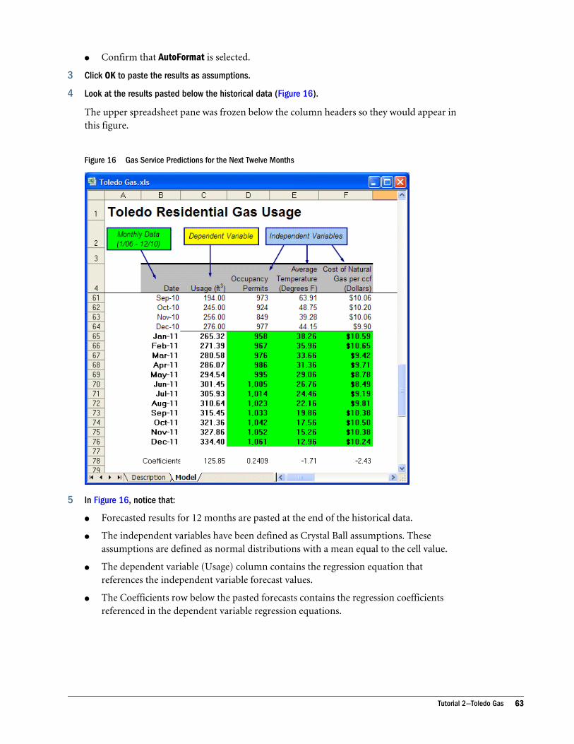
l Confirm that AutoFormat is selected.

3 Click OK to paste the results as assumptions.

4 Look at the results pasted below the historical data (Figure 16).

The upper spreadsheet pane was frozen below the column headers so they would appear inthis figure.

Figure 16 Gas Service Predictions for the Next Twelve Months

5 In Figure 16, notice that:

l Forecasted results for 12 months are pasted at the end of the historical data.

l The independent variables have been defined as Crystal Ball assumptions. Theseassumptions are defined as normal distributions with a mean equal to the cell value.

l The dependent variable (Usage) column contains the regression equation thatreferences the independent variable forecast values.

l The Coefficients row below the pasted forecasts contains the regression coefficientsreferenced in the dependent variable regression equations.


Creating a Report of Predictor Results

ä To create a report of Predictor data for each series:

1 Display the Predictor Results window.

If it is not visible, click Predictor Results in the Windows task bar. (It may be in the MicrosoftOffice Excel group.)

2 In the Predictor Results window menu bar, select Analyze, and then Create Report.

3 In the Create Report Preferences dialog, confirm that Predictor is selected and then click OK.

By default, the report is created in a separate workbook. The report contains summary datafollowed by information for each dependent and independent variable.

4 Click the Report workbook and scroll to the Average Temperature section (Figure 17).


Figure 17 Average Temperature Data Report for Toledo Gas

Notice the indication above the chart that the method used was an override of the bestmethod.

Extracting ResultsYou can extract results and methods data from the current Predictor forecasting run.


ä To extract Predictor results:



2 In the Predictor Results window menu bar, select Analyze, and then Extract Data.

3 In the Extract Data Preferences dialog, select the Predictor Data tab, if it is not already visible, andselect Results Table and Methods Table. Leave the defaults selected to extract all available data.

4 Select Options and confirm that the defaults are selected: New workbook, with sheet names ResultsTable and Methods Table, using AutoFormat.

5 Click OK.

A new Microsoft Excel workbook opens with two tabs, Results Table and Methods Table.Each tab contains an interactive Microsoft Excel PivotTable:

l Results Table shows fit values and residuals for historical data, plus forecast andconfidence interval values for the forecasted values. (Residuals are the differencebetween the data value and the calculated best fit value). By default, data seasons (cycles)appear as alternating bands of white and a light color. To hide these bands, you canreturn to the Results Window, select Preferences, and then clear Highlight Seasonality.

l Methods Table shows error calculations and other statistics for each selected fit method.

See “Extracting Results Data” on page 50.

Working with Data in Interactive Tables

ä To work with Predictor data in interactive tables:

1 Select the Methods Table worksheet.


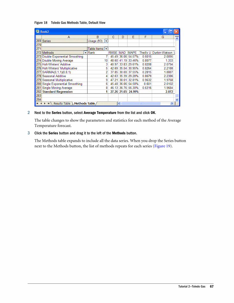
Figure 18 Toledo Gas Methods Table, Default View

2 Next to the Series button, select Average Temperature from the list and click OK.

The table changes to show the parameters and statistics for each method of the AverageTemperature forecast.

3 Click the Series button and drag it to the left of the Methods button.

The Methods table expands to include all the data series. When you drop the Series buttonnext to the Methods button, the list of methods repeats for each series (Figure 19).


Figure 19 Methods Grouped by Series

4 Click the arrow to the right of the Table Items button.

A list of fields is displayed.

5 Clear all the items except for Rank and click OK.

The Methods table changes to show the Rank parameter. Look at the Average Temperaturedata. In the Methods column, Double Moving Average is labeled Best method andhighlighted in bold text to show that it was used to generate the results. Seasonal Additive,originally the best, is still listed with a rank of 1 (Figure 20).


Figure 20 Methods Within each Series Identified by Rank

6 Move the Methods button to the left of the Series button.

The interactive Microsoft Excel PivotTable reorganizes to show all the series grouped bymethod type as shown in Figure 21.


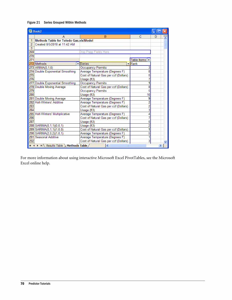
Figure 21 Series Grouped Within Methods

For more information about using interactive Microsoft Excel PivotTables, see the MicrosoftExcel online help.


BPredictor Examples

In This Appendix

About These Examples ... . . . . . . . . . . . . . . . . . . . . . . . . . . . . . . . . . . . . . . . . . . . . . . . . . . . . . . . . . . . . . . . . . . . . . . . . . . . . . . . . .71

Inventory Control . . . . . . . . . . . . . . . . . . . . . . . . . . . . . . . . . . . . . . . . . . . . . . . . . . . . . . . . . . . . . . . . . . . . . . . . . . . . . . . . . . . . . . . . . . .72

Company Finances... . . . . . . . . . . . . . . . . . . . . . . . . . . . . . . . . . . . . . . . . . . . . . . . . . . . . . . . . . . . . . . . . . . . . . . . . . . . . . . . . . . . . . .74

Human Resources ... . . . . . . . . . . . . . . . . . . . . . . . . . . . . . . . . . . . . . . . . . . . . . . . . . . . . . . . . . . . . . . . . . . . . . . . . . . . . . . . . . . . . . .77

About These ExamplesMonica’s Bakery, a hypothetical company used in the Predictor examples, is a rapidly growingbakery in Albuquerque, New Mexico. Since the opening, Monica has kept careful records (in aMicrosoft Excel workbook) of the sales of her three main products: French bread, Italian bread,and pizza. With these records, she can better predict her sales, control her inventory, market herproducts, and make strategic, long-term decisions.

ä To open Monica’s workbook, select Help, then Crystal Ball, then Examples Guide, and thenselect Monica's Bakery. (In Microsoft Excel 2007 or later, select Resources in the Help groupand then select Examples Guide).

The workbook has worksheets for sales data, operations, and cash flow. The Sales Data worksheetcontains all the historical sales data that is available for forecasting. The Operations worksheetcalculates the amount of different ingredients required to make different quantities of threebreads. The Cash Flow worksheet calculates how much money the bakery has to spend on variouscapital projects. The Labor Costs worksheet estimates the increase in hourly wages to decidewhether to invest in labor-saving equipment.

The following examples track Monica's decision-making processes as she uses Predictor to workthrough both short-term and long-term decisions:

l “Inventory Control” on page 72

l “Company Finances” on page 74

l “Human Resources” on page 77

For more detailed product tutorials, see Appendix A, “Predictor Tutorials.”

About These Examples 71

Inventory ControlThe initial reason that Monica needs to forecast is to maintain enough ingredients to keep upwith production. Monica's distributors give her discounts for buying in bulk. However, she mustbalance this savings with maintaining product quality, which requires using the freshestingredients possible. Monica wants improved forecasting to help her place orders that give herthe best volume pricing while maintaining the quality of her products.

To follow along with this example, open Bakery.xls as described in “About These Examples” onpage 71.

The Sales Data worksheet (Figure 22) shows the daily sales data of each of these products fromthe opening until the end of June 2010.

Figure 22 Bakery Sales Data Worksheet

A summary of data for the three main products by week is displayed at the bottom of theOperations worksheet (Figure 23). Monica can change the table to summarize her results byproduct, by time period, and more.

72 Predictor Examples

Figure 23 Bakery Operations Worksheet

Monica wants to order monthly, one month in advance. The bakery has already received thismonth’s delivery, which she placed last month. This month, she must place the order that willbe delivered at the end of this month for the next month, so she must forecast sales for the nexttwo months. Because she is in week 173 of her business, the forecast is for weeks 174 to 181.

ä To forecast the sales for weeks 174 to 181:

1 In the Bakery.xls workbook, click the Operations tab.

The Operations worksheet is displayed.

2 Select one cell—for example, C41—in the Historical Demand By Week table at the bottom of theworksheet.

3 Start Predictor.

Predictor automatically selects all the data in that table.

4 Ensure that:

l The cell range $B$40:$E$213 is selected correctly on the Input Data panel, with headers,dates, and data in columns settings also selected

l The Data Attributes panel shows time periods are in weeks with Seasonality set toAutoDetect

l In the Methods panel, Multiple Linear Regression is cleared and all time-series methodsare selected

l Options settings are the defaults, RMSE and Standard forecasting

5 Click Run.

6 In the Predictor Results window, set Periods to forecast to 8, and then click Paste.

Inventory Control 73

7 In the Paste Forecasts to Spreadsheet dialog, use the following settings and click OK:

l Select At end of historical data to indicate where to paste results.

l Select Include date series to list dates in the first column.

l Select Paste forecasts as Crystal Ball assumptions.

l Confirm that AutoFormat is selected.

The results paste to the end of the Historical Demand table as shown in Figure 24.

Figure 24 Forecasted Bakery Operations Results

The last four weeks of forecast values for each data series are automatically summed and placedinto the table at the top of the spreadsheet, in the Sales Forecast column (cells C9:C11). In thistable, the monthly sales forecast is converted to the number of items sold and then into theweight of each product.

The second table (below this top table) takes the total weight of each product (in cells C15, C19,C23) and calculates how much of each ingredient is required to produce that much product.The ingredients for each are then summed in the third table (below the second table) into thetotal amounts to order for the month (cells D31 to D34).

Based on the forecast, Monica should order:

l 12,080 pounds of flour

l 55 pounds of yeast

l 42 pounds of salt

l 125 pounds of tomatoes

Company FinancesMonica is always concerned about the bakery’s month-to-month cash flow (on a percent of salesbasis). Predictor can help her manage her inventory, and she can use it to predict her revenue


and understand her cash flow situation better. Understanding the bakery’s cash flow can, in turn,help her better manage major capital expenditures.

Monica is considering two major capital expenditures: a flour silo and a delivery van. She wantsto start construction on the silo in July and purchase the delivery van in August. She needs toforecast when the bakery can safely pay for these projects or whether the bakery must financethem.

To follow along with this example, open Bakery.xls as described in “About These Examples” onpage 71. If Bakery.xls is already open from the previous example, select Run, Reset to clear anyexisting results.

Note: Any pasted data will remain until you clear it in Microsoft Excel.

The bakery cash flow information is laid out in the Cash Flow worksheet, shown in Figure 25.

Figure 25 Bakery Cash Flow Worksheet

This worksheet has a table at the bottom that summarizes the sales data for the bakery’s threemain products by month. You can forecast the next three months of revenue to decide when toattempt the capital expenditures.

Company Finances 75

ä To forecast the next three months of revenue:

1 In the Bakery.xls workbook, click the Cash Flow tab.

The Cash Flow worksheet is displayed.

2 Select one cell—C36, for example—in the Historical Revenue By Month table at the bottom of theworksheet.

3 Start Predictor.

Predictor automatically selects all the data in the Historical Revenue table.

4 Confirm the following settings:

l In the Input Data panel, the cell range $C$36:$AP$36 is selected correctly, with Data inrows selected and no date or header settings selected.

l In Data Attributes, the first setting is Data is in periods with Seasonality set toAutoDetect.

l In Methods, all time-series methods are selected and Multiple Linear Regression iscleared (if available).

l Options settings are the defaults: RMSE and Standard forecasting.

5 Click Run.

6 In the Predictor Results window, enter 3 for Periods to forecast.

7 Click Paste, and then, in the Paste Forecasts to Spreadsheet dialog, confirm that results are set topaste at the end of historical data as Crystal Ball assumptions and click OK.

The results paste into the table at the bottom of the worksheet, cells AQ36 to AS36, and alsoappear at the top of the worksheet (cells E4 to G4) as shown in Figure 26.


Figure 26 Monthly Net Cash Flow Results

The revenue forecasts for the next three months are used to calculate the percentage expensesin the second table.

The second table calculates the total expenses, and the third table calculates the necessaryexpenditure for each extraordinary item. Below these tables is the cash flow summary for thenext three months, based on the forecasts. The net cash at the end of each month is what Monicais looking for (row 27). Based on forecasted sales, the new net cash values are $19,536.34 forJuly, $11,833.04 for August, and $35,452.31 for September. Based on the forecast, the bakeryshould wait until September to buy the van.

Human ResourcesMonica's Bakery is a labor-intensive operation that pays a competitive wage. However, tomaintain her target profitability, Monica must control labor costs. She knows there are manythings done around the bakery that could be done by expensive machinery, such as kneading,mixing, and forming. By accurately predicting her labor costs, she can decide when to invest insome of this equipment to keep her total expenses within budget.

Human Resources 77

From her interest in economics, Monica knows that a few key macro-economic figures drivelabor costs, such as the Industrial Production Index, local CPI, and local unemployment. All ofthese figures are available on the Internet on a monthly basis from the Bureau of Labor Statisticsand the Department of Commerce.

To follow along with this example, open Bakery.xls as described in “About These Examples” onpage 71. If Bakery.xls is already open from the previous example, select Run, and then Reset toclear existing results.

Monica has created her Labor Costs worksheet with an interactive table at the bottom that liststhe bakery's average hourly wage for each month and the monthly numbers for the threeeconomic indicators.

Figure 27 Bakery Labor Costs worksheet

The average hourly wage depends on or is affected by the other three variables. Because of thedependency, Monica decides to use regression instead of time-series forecasting. For regression,the dependent variable is Monica’s Average Wage, and the other three are the independentvariables.

ä To forecast the hourly wage using regression:

1 In the Bakery.xls workbook, click the Labor Costs tab.

The Labor Costs worksheet opens.

2 Select one cell—for example, C14—in the Economic Variables for Regression Analysis table at the topof the worksheet.

3 Start Predictor.

4 Ensure that:

l In Input Data, the cell range $B$13:$F$50 is selected correctly, with data in columns,header, and date settings also selected


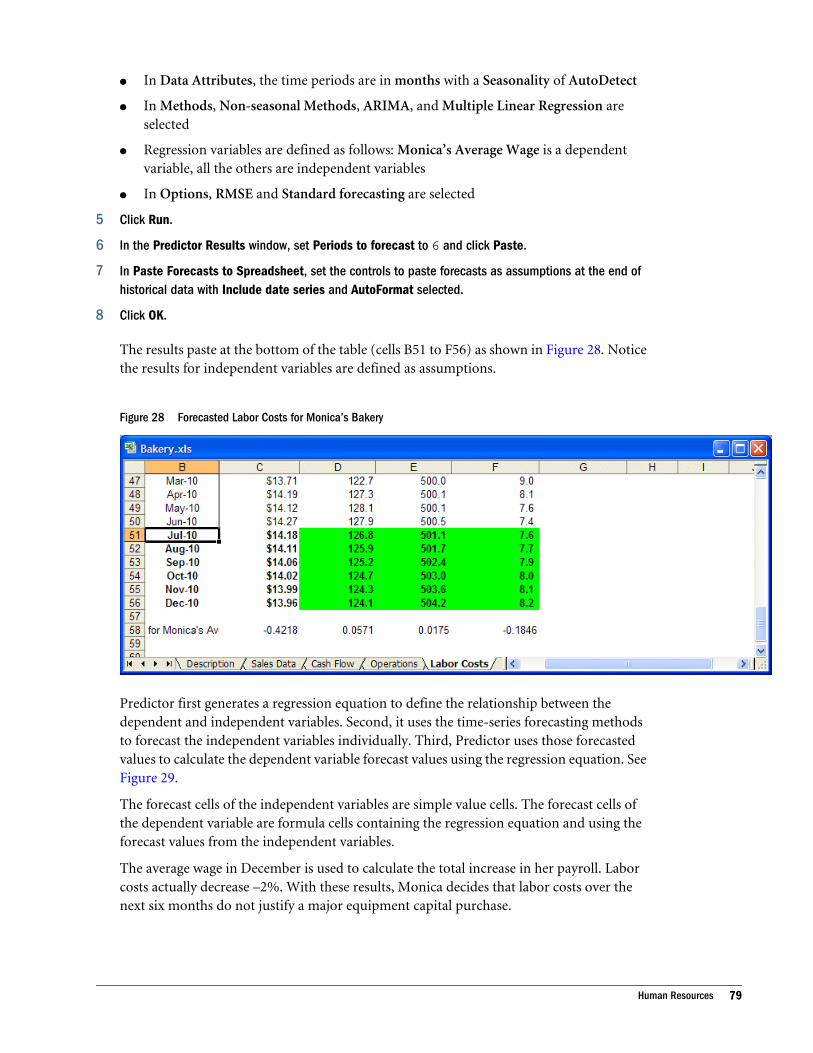
l In Data Attributes, the time periods are in months with a Seasonality of AutoDetect

l In Methods, Non-seasonal Methods, ARIMA, and Multiple Linear Regression areselected

l Regression variables are defined as follows: Monica’s Average Wage is a dependentvariable, all the others are independent variables

l In Options, RMSE and Standard forecasting are selected

5 Click Run.

6 In the Predictor Results window, set Periods to forecast to 6 and click Paste.

7 In Paste Forecasts to Spreadsheet, set the controls to paste forecasts as assumptions at the end ofhistorical data with Include date series and AutoFormat selected.

8 Click OK.

The results paste at the bottom of the table (cells B51 to F56) as shown in Figure 28. Noticethe results for independent variables are defined as assumptions.

Figure 28 Forecasted Labor Costs for Monica’s Bakery

Predictor first generates a regression equation to define the relationship between thedependent and independent variables. Second, it uses the time-series forecasting methodsto forecast the independent variables individually. Third, Predictor uses those forecastedvalues to calculate the dependent variable forecast values using the regression equation. SeeFigure 29.

The forecast cells of the independent variables are simple value cells. The forecast cells ofthe dependent variable are formula cells containing the regression equation and using theforecast values from the independent variables.

The average wage in December is used to calculate the total increase in her payroll. Laborcosts actually decrease –2%. With these results, Monica decides that labor costs over thenext six months do not justify a major equipment capital purchase.

Human Resources 79

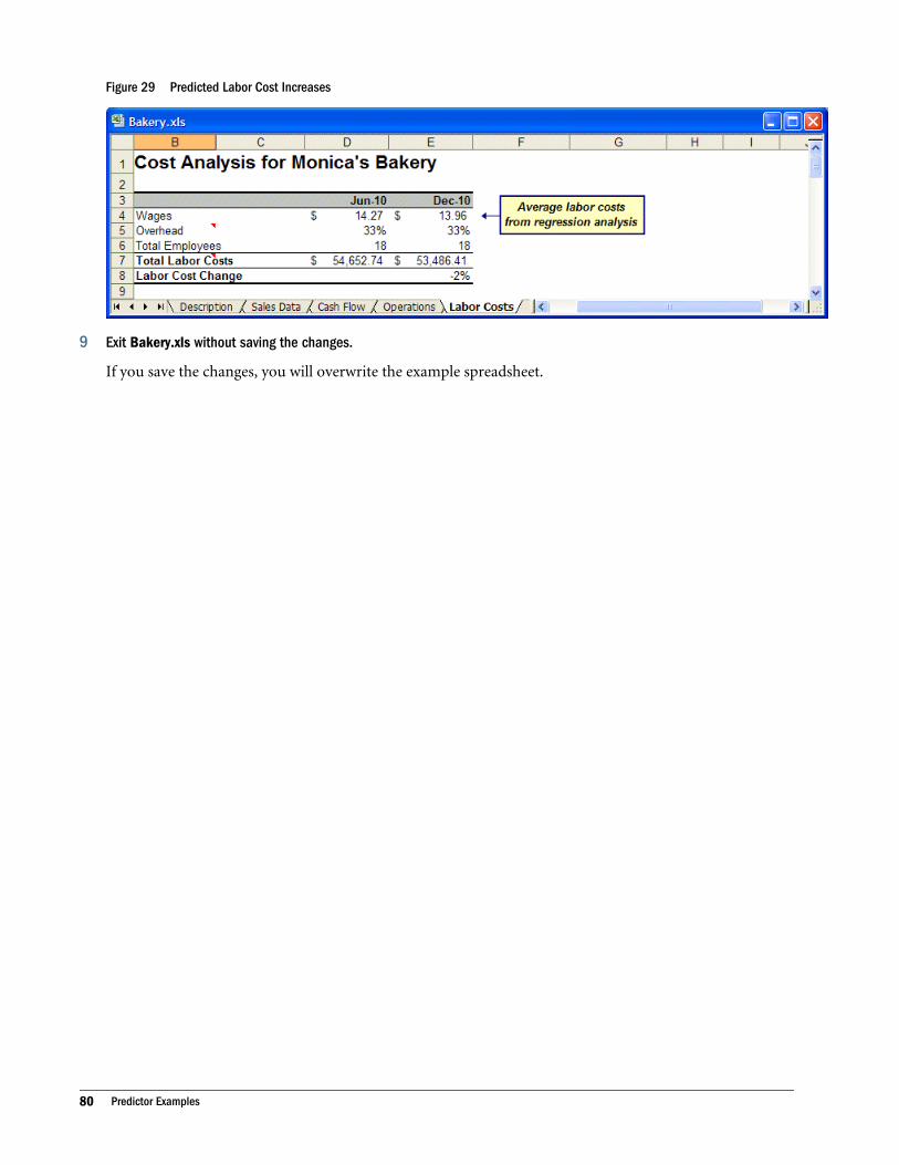
Figure 29 Predicted Labor Cost Increases

9 Exit Bakery.xls without saving the changes.

If you save the changes, you will overwrite the example spreadsheet.


CImportant Predictor Concepts

In This Appendix

About Forecasting Concepts .. . . . . . . . . . . . . . . . . . . . . . . . . . . . . . . . . . . . . . . . . . . . . . . . . . . . . . . . . . . . . . . . . . . . . . . . . . . . .81

Classic Time-series Forecasting... . . . . . . . . . . . . . . . . . . . . . . . . . . . . . . . . . . . . . . . . . . . . . . . . . . . . . . . . . . . . . . . . . . . . . . . .82

Time-series Forecasting Accuracy Measures ... . . . . . . . . . . . . . . . . . . . . . . . . . . . . . . . . . . . . . . . . . . . . . . . . . . . . . . . . .88

Time-series Forecasting Techniques... . . . . . . . . . . . . . . . . . . . . . . . . . . . . . . . . . . . . . . . . . . . . . . . . . . . . . . . . . . . . . . . . . . .90

Multiple Linear Regression ... . . . . . . . . . . . . . . . . . . . . . . . . . . . . . . . . . . . . . . . . . . . . . . . . . . . . . . . . . . . . . . . . . . . . . . . . . . . . .92

Regression Methods ... . . . . . . . . . . . . . . . . . . . . . . . . . . . . . . . . . . . . . . . . . . . . . . . . . . . . . . . . . . . . . . . . . . . . . . . . . . . . . . . . . . . .93

Regression Statistics.. . . . . . . . . . . . . . . . . . . . . . . . . . . . . . . . . . . . . . . . . . . . . . . . . . . . . . . . . . . . . . . . . . . . . . . . . . . . . . . . . . . . . .95

Historical Data Statistics .. . . . . . . . . . . . . . . . . . . . . . . . . . . . . . . . . . . . . . . . . . . . . . . . . . . . . . . . . . . . . . . . . . . . . . . . . . . . . . . . .96

Data Screening and Adjustment Methods ... . . . . . . . . . . . . . . . . . . . . . . . . . . . . . . . . . . . . . . . . . . . . . . . . . . . . . . . . . . . .97

About Forecasting ConceptsThis appendix describes forecasting terminology. It defines the time-series forecasting methodsthat Predictor uses, as well as other forecasting-related terminology. This appendix also describesthe statistics the program generates and the techniques that Predictor uses to do the calculationsand select the best-fitting method.

Forecasting refers to the act of predicting the future, usually for planning and managingresources. There are many scientific approaches to forecasting. You can perform “what-if”forecasting by creating a model and simulating outcomes, as with Crystal Ball, or by collectingdata over time and analyzing the trends and patterns. Predictor uses the latter concept, analyzingthe patterns of a time series to forecast future data.

The scientific approaches to forecasting usually fall into one of several categories:

l Time-series — Performs time-series analysis on past patterns of data to forecast results. Thisworks best for stable situations in which conditions are expected to remain the same.

l Regression — Forecasts results using past relationships between a variable of interest andseveral other variables that might influence it. This works best for situations in which youneed to identify the different effects of different variables. This category includes multiplelinear regression.

l Simulation — Randomly generates many scenarios for a model to forecast the possibleoutcomes. This method works best where you may not have historical data, but you canbuild the model of the situation to analyze its behavior.

About Forecasting Concepts 81

l Qualitative — Uses subjective judgment and expert opinion to forecast results. Thesemethods work best for situations for which no historical data or models are available.

Predictor uses time-series and multiple linear regression for forecasting. Oracle Crystal Ball,Fusion Edition uses simulation. Each technique and method has advantages and disadvantagesfor particular types of data, so often you might forecast the data using several methods and thenselect the method that yields the best results.

The following section, “Classic Time-series Forecasting” on page 82, describes forecastmethods available in Predictor and their uses.

These sections offer information about other data and forecast methodologies:

l “Multiple Linear Regression” on page 92

l “Historical Data Statistics” on page 96

Classic Time-series Forecasting

Subtopics

l Classic Non-seasonal Forecasting Methods

l Classic Seasonal Forecasting Methods

This section provides more information about classic time-series forecasting methods used inPredictor and described in “Using Classic Time-series Forecasting Methods” on page 30.Information about ARIMA (also known as Box-Jenkins) time-series forecasting methods arefound in “Using ARIMA Time-series Forecasting Methods” on page 33.

Time-series forecasting assumes that historical data is a combination of a pattern and somerandom error. Its goal is to isolate the pattern from the error by understanding the pattern’slevel, trend, and seasonality. You can then measure the error using a statistical measurement todescribe both how well a pattern reproduces historical data and to estimate how accurately itprojects the data into the future. See “Time-series Forecasting Accuracy Measures” on page88.

By default, Predictor tries all of the classic time-series methods in the Methods Gallery. It thenranks them according to which method has the lowest error, depending on the error measureselected in the Options pane. The method with the lowest error is the best method.

There are two primary techniques of classic time-series forecasting used in Predictor:

l “Classic Non-seasonal Forecasting Method Parameters” on page 85 — Estimate a trendby removing extreme data and reducing data randomness

l “Classic Seasonal Forecasting Methods” on page 85 — Combine forecasting data with anadjustment for seasonal behavior

For information about regression forecasting methods, see “Multiple Linear Regression” on page92. See the Oracle Crystal Ball Statistical Guide for more information about the formulas

82 Important Predictor Concepts

Predictor uses for the non-seasonal and seasonal forecasting methods described in the followingsections.

Classic Non-seasonal Forecasting MethodsNon-seasonal methods attempt to forecast by removing extreme changes in past data whererepeating cycles of data values are not present. The following classic non-seasonal forecastingmethods are available:

l “Single Moving Average (SMA)” on page 83

l “Double Moving Average (DMA)” on page 83

l “Single Exponential Smoothing (SES)” on page 84

l “Double Exponential Smoothing (DES)” on page 84

For information about associated parameters, see “Classic Non-seasonal Forecasting MethodParameters” on page 85.

Single Moving Average (SMA)Smooths historical data by averaging the last several periods and projecting the last average valueforward. Predictor can automatically calculate the optimal number of periods to average, or youcan select the number of periods to average.

This method is best for volatile data with no trend or seasonality. It results in a straight, flat-lineforecast.

Figure 30 Typical Single Moving Average Data, Fit, and Forecast Line

Double Moving Average (DMA)Applies the moving average technique twice, once to the original data and then to the resultingsingle moving average data. This method then uses both sets of smoothed data to project forward.Predictor can automatically calculate the optimal number of periods to average, or you can selectthe number of periods to average.

This method is best for historical data with a trend but no seasonality. It results in a straight,sloped-line forecast.

Classic Time-series Forecasting 83

Figure 31 Typical Double Moving Average Data, Fit, and Forecast Line

Single Exponential Smoothing (SES)Weights all of the past data with exponentially decreasing weights going into the past. In otherwords, usually the more recent data has greater weight. Weighting in this way largely overcomesthe limitations of moving averages or percentage change methods. Predictor can automaticallycalculate the optimal smoothing constant, or you can manually define the smoothing constant.

This method, which results in a straight, flat-line forecast is best for volatile data with no trendor seasonality.

Figure 32 Typical Single Exponential Smoothing Data, Fit, and Forecast Line

Double Exponential Smoothing (DES)Applies SES twice, once to the original data and then to the resulting SES data. Predictor usesHolt’s method for double exponential smoothing, which can use a different parameter for thesecond application of the SES equation. Predictor can automatically calculate the optimalsmoothing constants, or you can manually define the smoothing constants.

This method is best for data with a trend but no seasonality. It results in a straight, sloped-lineforecast.


Figure 33 Typical Double Exponential Smoothing Data, Fit, and Forecast Line

Classic Non-seasonal Forecasting Method ParametersThe classic non-seasonal methods use several forecasting parameters. For the moving averagemethods, the formulas use one parameter, period. When performing a moving average,Predictor averages over a number of periods. For single moving average, the number of periodscan be any whole number between 1 and half the number of data points. For double movingaverage, the number of periods can be any whole number between 2 and one-third the numberof data points.

For single exponential smoothing, there is one parameter: alpha. Alpha (a) is the smoothingconstant. The value of alpha can be any number between 0 and 1, not inclusive.

For double exponential smoothing, there are two parameters: alpha and beta. Alpha is the samesmoothing constant as described above for single exponential smoothing. Beta (b) is also asmoothing constant exactly like alpha except that it is used during second smoothing. The valueof beta can be any number between 0 and 1, not inclusive.

Classic Seasonal Forecasting MethodsSeasonal forecasting methods extend the non-seasonal forecasting methods by adding anadditional component to capture the seasonal behavior of the data. Predictor offers four classicseasonal forecasting methods:

l “Seasonal Additive” on page 86

l “Seasonal Multiplicative” on page 86

l “Holt-Winters’ Additive” on page 86

l “Holt-Winters’ Multiplicative” on page 87

For associated parameters, see “Classic Seasonal Forecasting Method Parameters” on page87.

See the Oracle Crystal Ball Statistical Guide for more information about the formulas Predictoruses.


Seasonal AdditiveCalculates a seasonal index for historical data that does not have a trend. The method producesexponentially smoothed values for the level of the forecast and the seasonal adjustment to theforecast. The seasonal adjustment is added to the forecasted level, producing the seasonaladditive forecast.

This method is best for data without trend but with seasonality that does not increase over time.It results in a curved forecast that reproduces the seasonal changes in the data.

Figure 34 Typical Seasonal Additive Data, Fit, and Forecast Curve without Trend

Seasonal MultiplicativeCalculates a seasonal index for historical data that does not have a trend. The method producesexponentially smoothed values for the level of the forecast and the seasonal adjustment to theforecast. The seasonal adjustment is multiplied by the forecasted level, producing the seasonalmultiplicative forecast.

This method is best for data without trend but with seasonality that increases or decreases overtime. It results in a curved forecast that reproduces the seasonal changes in the data.

Figure 35 Typical Seasonal Multiplicative Data, Fit, and Forecast Curve without Trend

Holt-Winters’ AdditiveIs an extension of Holt's exponential smoothing that captures seasonality. This method is basedupon three equations that can be found in the Oracle Crystal Ball Statistical Guide. The methodproduces exponentially smoothed values for the level of the forecast, the trend of the forecast,


and the seasonal adjustment to the forecast. This seasonal additive method adds the seasonalityfactor to the trended forecast, producing the Holt-Winters’ additive forecast.

This method is best for data with trend and seasonality that does not increase over time. It resultsin a curved forecast that shows the seasonal changes in the data.

Figure 36 Typical Holt-Winters’ Additive Data, Fit, and Forecast Curve

Holt-Winters’ MultiplicativeIs similar to the Holt-Winters’ additive method. Holt-Winters’ Multiplicative method alsocalculates exponentially smoothed values for level, trend, and seasonal adjustment to theforecast. This method's equations can also be found in the Oracle Crystal Ball Statistical Guide.This seasonal multiplicative method multiplies the trended forecast by the seasonality,producing the Holt-Winters’ multiplicative forecast.

This method is best for data with trend and with seasonality that increases over time. It resultsin a curved forecast that reproduces the seasonal changes in the data.

Figure 37 Typical Holt-Winters’ Multiplicative Data, Fit, and Forecast Curve

Classic Seasonal Forecasting Method ParametersThe seasonal forecast methods use three smoothing parameters: alpha, beta, and gamma:

l alpha (α) — Smoothing parameter for the level component of the forecast. The value ofalpha can be any number between 0 and 1, not inclusive.

l beta (β) — Smoothing parameter for the trend component of the forecast. The value ofbeta can be any number between 0 and 1, not inclusive.


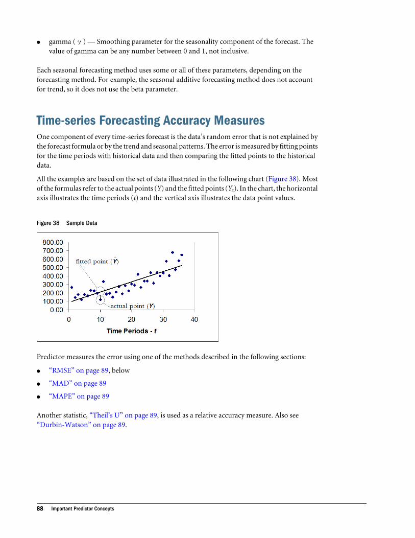
l gamma (γ) — Smoothing parameter for the seasonality component of the forecast. Thevalue of gamma can be any number between 0 and 1, not inclusive.

Each seasonal forecasting method uses some or all of these parameters, depending on theforecasting method. For example, the seasonal additive forecasting method does not accountfor trend, so it does not use the beta parameter.

Time-series Forecasting Accuracy MeasuresOne component of every time-series forecast is the data’s random error that is not explained bythe forecast formula or by the trend and seasonal patterns. The error is measured by fitting pointsfor the time periods with historical data and then comparing the fitted points to the historicaldata.

All the examples are based on the set of data illustrated in the following chart (Figure 38). Mostof the formulas refer to the actual points (Y) and the fitted points (Yt). In the chart, the horizontalaxis illustrates the time periods (t) and the vertical axis illustrates the data point values.

Figure 38 Sample Data

Predictor measures the error using one of the methods described in the following sections:

l “RMSE” on page 89, below

l “MAD” on page 89

l “MAPE” on page 89

Another statistic, “Theil’s U” on page 89, is used as a relative accuracy measure. Also see“Durbin-Watson” on page 89.


RMSERMSE (root mean squared error) is an absolute error measure that squares the deviations tokeep the positive and negative deviations from cancelling out one another. This measure alsotends to exaggerate large errors, which can help eliminate methods with large errors.

MADMAD (mean absolute deviation) is an absolute error measure that originally became verypopular (in the days before hand-held calculators) because it didn’t require the calculation ofsquares or square roots. While it is still fairly reliable and widely used, it is most accurate fornormally distributed data.

MAPEMAPE (mean absolute percentage error) is a relative error measure that uses absolute values.There are two advantages of this measure. First, the absolute values keep the positive and negativeerrors from cancelling out each other. Second, because relative errors do not depend on the scaleof the dependent variable, this measure lets you compare forecast accuracy between differentlyscaled time-series data.

Theil’s UTheil’s U statistic is a relative accuracy measure that compares the forecasted results with a naiveforecast. It also squares the deviations to give more weight to large errors and to exaggerateerrors, which can help eliminate methods with large errors (Table 3). For the formula, see theOracle Crystal Ball Statistical Guide.

Table 3 Interpreting Theil’s U

Theil’s U Statistic Interpretation

Less than 1 The forecasting technique is better than guessing.

1 The forecasting technique is about as good as guessing.

More than 1 The forecasting technique is worse than guessing.

Durbin-WatsonDetects autocorrelation at lag 1. This means that each time-series value influences the next value.This is the most common type of autocorrelation.For the formula, see the Oracle Crystal BallStatistical Guide.

This statistic can have any value between 0 and 4. Values indicate slow-moving, none, or fast-moving autocorrelation (Table 4).

Time-series Forecasting Accuracy Measures 89

Table 4 Interpreting the Durbin Watson Statistic

Durbin-Watson Statistic Interpretation

Less than 1 The errors are positively correlated. An increase in one period follows an increase in the previous period.

2 No autocorrelation.

More than 3 The errors are negatively correlated. An increase in one period follows a decrease in the previous period.

Avoid using independent variables that have errors with a strong positive or negative correlation,because this can lead to an incorrect forecast for the dependent variable.

Time-series Forecasting Techniques

Subtopics

l Standard Forecasting

l Simple Lead Forecasting

l Weighted Lead Forecasting

l Holdout Forecasting

Predictor uses one of four forecasting techniques to perform time-series forecasting:

l “Standard Forecasting” on page 90

l “Simple Lead Forecasting” on page 91

l “Weighted Lead Forecasting” on page 91

l “Holdout Forecasting” on page 91

Classic time-series forecasting methods can use any of these techniques, but ARIMA methodscan use only Standard and Holdout forecasting.

Standard ForecastingStandard forecasting optimizes the forecasting parameters to minimize the error measurebetween the fit values and the historical data for the same period. For example, considerTable 5 showing historical data and calculated fit values for periods 1 through 7.

Table 5 Example of Historical Data and Fit with Standard Forecasting

Period Historical Data Value Fit Value

1 472 488

2 599 609

3 714 702

4 892 888


Period Historical Data Value Fit Value

5 874 890

6 896 909

7 890 870

Predictor calculates the RMSE using the differences between the historical data and the fit datafrom the same periods. For example:

(472-488)2 + (599-609)2 + (714-702)2 + (892-888)2 + ...

For standard forecasting, Predictor optimizes the forecasting parameters so that the RMSEcalculated in this way is minimized.

Simple Lead ForecastingSimple lead forecasting optimizes the forecasting parameters to minimize the error measurebetween the historical data and the fit values, offset by a specified number of periods (lead). Usethis forecasting technique when a forecast for some future time period has the greatestimportance, more so than the forecasts for the previous or later periods. For example, singlelead forecasting can be used if your company must order extremely expensive manufacturingcomponents two months in advance, making any forecast for two months out the mostimportant.

Weighted Lead ForecastingWeighted lead forecasting optimizes the forecasting parameters to minimize the average errormeasure between the historical data and the fit values, offset by 0, 1, 2, and so on, up to thespecified number of periods (weighted lead). It uses the simple lead technique for several leadperiods and then averages the forecast over the periods, optimizing this average value. Use thistechnique when the future forecast for several periods is most important. For example, weightedlead forecasting can be used if your company must order extremely expensive manufacturingcomponents zero, one, and two months in advance, making any forecast for all the time periodsup to two months out the most important.

Holdout ForecastingHoldout forecasting:

1. Removes the last few data points of the historical data.

2. Calculates the fit and forecast points using the remaining historical data.

3. Compares the error between the forecasted points and their corresponding, excluded,historical data points.

4. Changes the parameters to minimize the error between the forecasted points and theexcluded points.

Time-series Forecasting Techniques 91

Predictor determines the optimal forecast parameters using only the non-holdout set of data.

Note that if you have a small amount of data and want to use seasonal forecasting methods,using the holdout technique might restrict you to non-seasonal methods.

For more information on the holdout technique and when to use it effectively, see theMakridakis, Wheelwright, and Hyndman reference in Appendix D, “Bibliography.”

Multiple Linear RegressionMultiple linear regression is used for data where one data series (the dependent variable) is afunction of, or depends on, other data series (the independent variables). For example, the yieldof a lettuce crop depends on the amount of water provided, the hours of sunlight each day, andthe amount of fertilizer used.

The goal of multiple linear regression is to find an equation that most closely matches thehistorical data. “Multiple” indicates that you can use more than one independent variable todefine the dependent variable in the regression equation. “Linear” indicates that the regressionequation is a linear equation.

The linear equation describes how the independent variables (x1, x2, x3,...) combine to definethe single dependent variable (y). Multiple linear regression finds the coefficients for theequation:

y = b0 + b1x1 + b2x2 + b3x3 + ... + e

where b1, b2, and b3, are the coefficients of the independent variables, b0 is the y-interceptconstant, and e is the error.

If there is only one independent variable, the equation defines a straight line. This uses a specialcase of multiple linear regression called simple linear regression, with the equation:

y = b0 + b1x + e

where b0 is where the regression line crosses the graph's y axis, x is the independent variable,and e is the error. When the regression equation has only two independent variables, it definesa plane. When the regression equation has more than two independent variables, it defines a hyperplane.

To find the coefficients of these equations, Predictor uses singular value decomposition. Formore information on this technique, see the Oracle Crystal Ball Statistical Guide.


Figure 39 Parts of a Scatter Plot

For more information on multiple linear regressions, see:

l “Regression Methods” on page 93

l “Regression Statistics” on page 95

Regression MethodsPredictor uses one of three methods for calculating multiple linear regression:

l “Standard Regression” on page 93

l “Forward Stepwise Regression” on page 93

l “Iterative Stepwise Regression” on page 94

Standard RegressionStandard regression performs multiple linear regression, generating regression coefficients foreach independent variable you specify, no matter how significant.

Forward Stepwise RegressionForward stepwise regression adds one independent variable at a time to the multiple linearregression equation, starting with the independent variable with the most significant probabilityof the correlation (partial F statistic). It then recalculates the partial F statistic for the remainingindependent variables, taking the existing regression equation into consideration.

The resulting multiple linear regression equation will always have at least one independentvariable.

Forward stepwise regression continues to add independent variables until either:

Regression Methods 93

l It runs out of independent variables.

l It reaches one of the selected stopping criteria in the Stepwise Options dialog.

l The number of included independent variables reaches one-third the number of data pointsin the series.

There are two stopping criteria:

l R-squared (R2) — Stops the stepwise regression if the difference between a specified statistic(either R2 or adjusted R2) for the previous and new regression solutions is below a thresholdvalue. When this happens, Predictor does not use the last independent variable. For example,the third step of a stepwise regression results in an R2 value of 0.81, and the fourth step addsanother independent variable and results in an R2 value is 0.83. The difference between theR2 values is 0.02. If the threshold value is 0.03, Predictor returns to the regression equationfor the third step and stops the stepwise regression.

l Partial F-test significance — Stops the stepwise regression if the probability of the partialF statistic for a new solution is above a maximum value. For example, if you set the maximumprobability to 0.05 and the partial F statistic for the fourth step of a stepwise regression resultsin a probability of 0.08, Predictor returns to the regression equation for the third step andstops the stepwise regression.

Iterative Stepwise RegressionIterative stepwise regression adds or removes one independent variable at a time to or from themultiple linear regression equation.

To perform iterative stepwise regression, Predictor:

1. Calculates the partial F statistic for each independent variable.

2. Adds the independent variable with the most significant correlation (partial F statistic).

3. Checks the partial F statistic of the independent variables in the regression equation to seeif any became insignificant (have a probability below the minimum) with the addition ofthe latest independent variable.

4. Removes the least significant of any insignificant independent variables one at a time.

5. Repeats step 3 until no insignificant variables remain in the regression equation.

6. Repeats steps 1 through 5 until one of the following occurs:

l The model runs out of independent variables.

l The regression reaches one of the stopping criteria (see the “Forward StepwiseRegression” on page 93 for information on how the stopping criteria work).

l The same independent variable is added and then removed.

The resulting equation always has at least one independent variable.


Regression StatisticsAfter Predictor finds the regression equation, it calculates several statistics to help you evaluatethe regression:

l “R2” on page 95

l “Adjusted R2” on page 95

l “Sum of Squared Errors (SSE)” on page 95

l “F statistic” on page 96

l “t statistic” on page 96

l “p” on page 96

See the Oracle Crystal Ball Statistical Guide for more information on the formulas Predictor usesto calculate these statistics.

R2

Coefficient of determination. This statistic indicates the percentage of the variability of thedependent variable that the regression equation explains.

For example, an R2 of 0.36 indicates that the regression equation accounts for 36% of thevariability of the dependent variable.

Adjusted R2

Corrects R2 to account for the degrees of freedom in the data. In other words, the more datapoints you have, the more universal the regression equation is. However, if you have only thesame number of data points as variables, the R2 might appear deceptively high. This statisticcorrects for that.

For example, the R2 for one equation might be very high, indicating that the equation accountedfor almost all the error in the data. However, this value might be inflated if the number of datapoints was insufficient to calculate a universal regression equation.

Sum of Squared Errors (SSE)The least squares technique for estimating regression coefficients minimizes this statistic, whichmeasures the error not eliminated by the regression line.

For any line drawn through a scatter plot of data, there are several ways to determine which linefits the data best. One method used to compare the fit of lines is to calculate the SSE (sum of thesquared errors, or deviations) for each line. The lower the SSE, the better the fit of the line tothe data.

Regression Statistics 95

F statisticTests the significance of the regression equation as measured by R2. A significant value meansthat the regression equation accounts for some of the variability of the dependent variable.

t statisticTests the significance of the relationship between the coefficients of the dependent variable andan individual independent variable, in the presence of the other independent variables. Asignificant value means that the independent variable contributes to the dependent variable.

pIndicates the probability of the calculated F or t statistic being as large as it is (or larger) bychance. A low p value is good and means that the F statistic is not coincidental and, therefore,is significant. A significant F statistic means that the relationship between the dependent variableand the combination of independent variables is significant.

Generally, p should be less than 0.05.

Historical Data StatisticsPredictor automatically calculates the following statistics for historical data series:

l “Mean” on page 96

l “Standard Deviation” on page 97

l “Minimum” on page 97

l “Maximum” on page 97

l “Ljung-Box Statistic” on page 97

If an ARIMA model is displayed in the Method box, the transformation lambda and threeselection criteria values are also included in the Statistics group. For more information aboutthese values, see “Using ARIMA Time-series Forecasting Methods” on page 33 and theBibliography.

MeanThe mean of a set of values is found by adding the values and dividing their sum by the numberof values. “Average” usually refers to the mean. For example, 5.2 is the mean or average of 1, 3,6, 7, and 9.


Standard DeviationThe standard deviation is the square root of the variance for a distribution. Like the variance, itis a measure of dispersion about the mean and is useful for describing the “average” deviation.

For example, you can calculate the standard deviation of the values 1, 3, 6, 7, and 9 by findingthe square root of the variance that is calculated in the variance example below.

The standard deviation, denoted as s, is calculated from the variance as follows:

where the variance is a measure of the dispersion, or spread, of a set of values about the mean.When values are close to the mean, the variance is small. When values are widely scattered aboutthe mean, the variance is larger.

MinimumThe minimum is the smallest value in the data range.

MaximumThe maximum is the largest value in the data range.

Ljung-Box StatisticMeasures whether a set of autocorrelations is significantly different from a set of autocorrelationsthat are all zero. See the Oracle Crystal Ball Statistical Guide for the formula.

Data Screening and Adjustment MethodsHistorical data can have missing values and outliers, which are data points that differ significantlyfrom the rest of the data. Settings in the Data Attributes panel of the Predictor wizard enableyou to select several ways of handling missing values and identifying and adjusting outliers.Because adjusted outliers are treated as missing values, both of these situations are discussed andhandled together.

“Setting Screening Options” on page 28 describes how to display the Screening Options dialog.The groups in this dialog list:

l “Outlier Detection Methods” on page 97

l “Outlier and Missing Value Adjustment Methods” on page 99

Outlier Detection MethodsPredictor offers three methods for detecting outliers, or significantly extreme values:

Data Screening and Adjustment Methods 97

l “Mean and Standard Deviation Method” on page 98

l “Median and Median Absolute Deviation Method (MAD)” on page 98

l “Median and Interquartile Deviation Method (IQD)” on page 98

In each case, the difference is calculated between historical data points and values calculated bythe various forecasting methods. These differences are called residuals. They can be positive ornegative depending on whether the historical value is greater than or less than the smoothedvalue. Various statistics are then calculated on the residuals and these are used to identify andscreen outliers.

A certain number of values must exist before the data fit can begin. If outliers appear at thebeginning of the data, they are not detected.

Note: Time-series data is typically treated differently from other data because of its dynamicnature, such as the pattern in the data. A time-series outlier need not be extreme withrespect to the total range of the data variation but it is extreme relative to the variationlocally.

Mean and Standard Deviation MethodFor this outlier detection method, the mean and standard deviation of the residuals are calculatedand compared. If a value is a certain number of standard deviations away from the mean, thatdata point is identified as an outlier. The specified number of standard deviations is called thethreshold. The default value is 3.

This method can fail to detect outliers because the outliers increase the standard deviation. Themore extreme the outlier, the more the standard deviation is affected.

Median and Median Absolute Deviation Method (MAD)For this outlier detection method, the median of the residuals is calculated. Then, the differenceis calculated between each historical value and this median. These differences are expressed astheir absolute values, and a new median is calculated and multiplied by an empirically derivedconstant to yield the median absolute deviation (MAD). If a value is a certain number of MADaway from the median of the residuals, that value is classified as an outlier. The default thresholdis 3 MAD.

This method is generally more effective than the mean and standard deviation method fordetecting outliers, but it can be too aggressive in classifying values that are not really extremelydifferent. Also, if more than 50% of the data points have the same value, MAD is computed tobe 0, so any value different from the residual median is classified as an outlier.

Median and Interquartile Deviation Method (IQD)For this outlier detection method, the median of the residuals is calculated, along with the 25thpercentile and the 75th percentile. The difference between the 25th and 75th percentile is theinterquartile deviation (IQD). Then, the difference is calculated between each historical value


and the residual median. If the historical value is a certain number of MAD away from the medianof the residuals, that value is classified as an outlier. The default threshold is 2.22, which isequivalent to 3 standard deviations or MADs.

This method is somewhat susceptible to influence from extreme outliers, but less so than themean and standard deviation method. Box plots are based on this approach. The median andinterquartile deviation method can be used for both symmetric and asymmetric data.

Outlier and Missing Value Adjustment MethodsPredictor provides two methods for filling in missing values and adjusting outliers:

l “Cubic Spline Interpolation Method” on page 99

l “Neighbor Interpolation Method” on page 99

Missing values at the beginning of a data series are ignored. Missing values at the end of a dataseries are allowed, but this condition is not ideal. The cubic spline interpolation method isespecially sensitive to data missing at the end of the series. If one or two values are missing, cubicspline interpolation can be used. If multiple values are missing, neighbor interpolation providesa better estimate.

Tip: An obvious outlier, such as a large data spike, should be replaced by a blank cell in theoriginal data set. Otherwise, neighbor interpolation is probably a better adjustment method,especially if the specified neighbors do not include the spike. Because cubic splineinterpolation takes into account the whole data set, that adjustment method will be affectedby the outlier.

Cubic Spline Interpolation MethodCubic spline interpolation is based on a drafting tool used to draw smooth curves through anumber of points. The spline tool consists of weights attached to a flat surface at the points tobe connected. A flexible strip is then bent across each of these weights, resulting in a smoothcurve.

The cubic spline interpolation is a piecewise continuous curve that passes through each valuein the data set. Each interval of the curve has a separate cubic polynomial, each with its owncoefficients. These are equivalent to the spline tool's weights. The cubic spline interpolationmethod considers the entire data set when adjusting outliers and filling in missing values.

Neighbor Interpolation MethodThis method is also called the single imputation method. A certain number of neighbors on eachside of the missing value are considered when estimating the missing value. This value is calledn, and the total number of neighbors evaluated is 2n. The missing data is replaced by the meanor median of the 2n data points. The default value for n is 1, and the default statistic is Mean.

Data Screening and Adjustment Methods 99

Note: To preserve the local nature of time series data, the number of neighbors on each side ofthe missing value or values should be small, ideally n = 1 or n = 2.


DBibliography

In This Appendix

Forecasting ... . . . . . . . . . . . . . . . . . . . . . . . . . . . . . . . . . . . . . . . . . . . . . . . . . . . . . . . . . . . . . . . . . . . . . . . . . . . . . . . . . . . . . . . . . . . . 101

ARIMA Forecasting ... . . . . . . . . . . . . . . . . . . . . . . . . . . . . . . . . . . . . . . . . . . . . . . . . . . . . . . . . . . . . . . . . . . . . . . . . . . . . . . . . . . . . 101

Regression Analysis.. . . . . . . . . . . . . . . . . . . . . . . . . . . . . . . . . . . . . . . . . . . . . . . . . . . . . . . . . . . . . . . . . . . . . . . . . . . . . . . . . . . . . 102

ForecastingBowerman, B.L., and R.T. O'Connell (contributor). Forecasting and Time Series: An AppliedApproach (The Duxbury Advanced Series in Statistics and Decision Sciences). Belmont, CA:Duxbury Press, 1993.

DeLurgio, S.A., Sr. Forecasting Principles and Applications. Boston: Irwin/McGraw-Hill, 1998.

Hanke, J.E., and D.W. Wichern. Business Forecasting. 9th ed. Upper Saddle River:, NJ: PrenticeHall, 2008.

Makridakis, S., S.C. Wheelwright, and R.J. Hyndman. Forecasting Methods and Applications. 3rded. Hoboken, NJ: John Wiley & Sons, 1998.

Ragsdale, C. Spreadsheet Modeling and Decision Analysis: A Practical Introduction to ManagementScience. 5th ed. Florence, KY: South-Western College Publishing, 2007.

Wei, W.W.S. Time Series Analysis: Univariate and Multivariate Methods. 2nd ed. New York:Pearson, 2006.

ARIMA ForecastingBox, G. E. P., Jenkins, G. M., and Reinsel, G. C. Time Series Analysis: Forecasting and Control.4th ed. Hoboken, NJ: John Wiley & Sons. 2008.

Hamilton, J. D. Time Series Analysis. Princeton, NJ: Princeton University Press. 1st ed. 1994.

Hanke, J.E., and D.W. Wichern. Business Forecasting. 9th ed. Upper Saddle River, NJ: PrenticeHall, 2008.

Liu, Lon-Mu. Time Series Analysis and Forecasting. 2nd ed. Villa Park, IL: Scientific ComputingAssociates. 2006.


Forecasting 101

Wei, W. W. S. Time Series Analysis: Univariate and Multivariate methods. 2nd ed. New York:Pearson, 2006.

Regression AnalysisDraper, N.R., and H. Smith. Applied Regression Analysis. 3rd ed. Hoboken, NJ: John Wiley &Sons, 1998.

Golub, G.H., and C.F. Van Loan. Matrix Computations, 3rd ed. Baltimore: The Johns HopkinsUniversity Press, 1996.

Hanke, J.E., and D.W. Wichern. Business Forecasting. 9th ed. Upper Saddle River, NJ: PrenticeHall, 2008.


Miller, A. Subset Selection in Regression. 2nd ed. Chapman & Hall/CRC, 2002.

102 Bibliography

Glossary

Adjusted R2 Corrects R2 to account for the degrees of

freedom in the data.

ARIMA Often called the Box-Jenkins forecasting

methodology, ARIMA is a set of univariate time-series

forecasting methods. ARIMA involves the identification,

selection, and checking of models with estimated

autoregressive (AR), integration or differencing (I), and

moving average (MA) parameters.

assumptions Estimated values in a spreadsheet model that

Crystal Ball defines with a probability distribution.

autocorrelation Describes a relationship or correlation

between values of the same data series at different time

periods.

autoregression Describes a relationship similar to

autocorrelation, except instead of the variable being related

to other independent variables, it is related to previous

values of its own data series.

causal methods A relationship between two variables where

changes in one independent variable not only correspond

to a particular increase or decrease in the dependent

variable, but actually cause the increase or decrease.

Crystal Ball forecast A statistical summary of the assumptions

in a spreadsheet model, output graphically or numerically.

degrees of freedom The number of data points minus the

number of estimated parameters (coefficients).

dependent variable In multiple linear regression, a data series

or variable that depends on another data series. You should

use multiple linear regression as the forecasting method for

any dependent variable.

DES Double exponential smoothing.

double exponential smoothing Double exponential smoothing

applies single exponential smoothing twice, once to the

original data and then to the resulting single exponential

smoothing data. It is useful where the historic data series is

not stationary.

double moving average Smooths out past data by performing

a moving average on a subset of data that represents a

moving average of an original set of data.

Durbin-Watson Tests for autocorrelation of one time lag.

error The difference between the actual data values and the

forecasted data values.

F statistic Tests the overall significance of the multiple linear

regression equation.

F-test statistic See F statistic.

forecast The prediction of values of a variables based on

known past values of that variable or other related variables.

Forecasts can also describe predicted values based on Crystal

Ball spreadsheet models and expert judgements.

forward stepwise A regression method that adds one

independent variable at a time to the multiple linear

regression equation, starting with the independent variable

with the greatest significance.

holdout Optimizes the forecasting parameters to minimize

the error measure between a set of excluded data and the

forecasting values. Predictor does not use the excluded data

to calculate the forecasting parameters.

Holt-Winters’ additive forecasting method Separates a series into

its component parts: seasonality, trend and cycle, and error.

This method determines the value of each, projects them

forward, and reassembles them to create a forecast.

Glossary 103

Holt-Winters’ multiplicative forecasting method Considers the

effects of seasonality to be multiplicative, that is, growing

(or decreasing) over time. This method is similar to the

Holt-Winters’ additive method.

hyperplane A geometric plane that spans more than two

dimensions.

independent variable In multiple linear regression, the data

series or variables that influence the another data series or

variable.

iterative stepwise regression A regression method that adds or

subtracts one independent variable at a time to or from the

multiple linear regression equation.

lag Defines the offset when comparing a data series with

itself. For autocorrelation, this refers to the offset of data

that you choose when correlating a data series with itself.

lead A type of forecasting that optimizes the forecasting

parameters to minimize the error measure between the

historical data and the fit values, offset by a specified number

of periods (lead).

least-squares approach Measures how closely a line matches

a set of data. This approach measures the distance of each

actual data point from the line, squares each distance, and

adds up the squares. The line with the smallest square

deviation is the closest fit.

level A starting point for the forecast. For a set of data with

no trend, this is equivalent to the y-intercept.

linear equation An equation with only linear terms. A linear

equation has no terms containing variables with exponents

or variables multiplied by each other.

linear regression A process that models a variable as a

function of other first-order explanatory variables. In other

words, it approximates the curve with a line, not a curve,

which would require higher-order terms involving squares

and cubes.

MAD Mean absolute deviation. This is an error statistic that

average distance between each pair of actual and fitted data

points.

MAPE Mean absolute percentage error. This is a relative

error measure that uses absolute values to keep the positive

and negative errors from cancelling out each other and uses

relative errors to let you compare forecast accuracy between

time-series methods.

multiple linear regression A case of linear regression where one

dependent variable is described as a linear function of more

than one independent variable.

naive forecast A forecast obtained with minimal effort based

on only the most recent data; e.g., using the last data point

to forecast the next period.

p Indicates the probability of obtaining an F or t statistic as

large as the one calculated for the data.

partial F statistic Tests the significance of a particular

independent variable within the existing multiple linear

regression equation.

PivotTable An interactive table in Microsoft Excel. You can

move rows and columns and filter PivotTable data.

R2 Coefficient of determination. This statistic indicates

what proportion of the dependent variable error that the

regression line explains.

regression A process that models a dependent variable as a

function of other explanatory (independent) variables.

residuals The difference between the actual data and the

predicted data for the dependent variable in multiple linear

regression.

RMSE Root mean squared error. This is an absolute error

measure that squares the deviations to keep the positive and

negative deviations from cancelling out each other. This

measure also tends to exaggerate large errors, which can help

when comparing methods.

seasonal additive forecasting method Calculates a seasonal

index for historical data that does not have a trend. The

seasonal adjustment is added to the forecasted level,

producing the seasonal additive forecast.

seasonal multiplicative forecasting method Calculates a seasonal

index for historical data that does not have a trend. The

seasonal adjustment is multiplied by the forecasted level,

producing the seasonal multiplicative forecast.

seasonality The change that seasonal factors cause in a data

series. For example, if sales increase during the Christmas

season and during the summer, the data is seasonal with a

six-month period.

104 Glossary

single exponential smoothing forecasting method (SES) Weights

past data with exponentially decreasing weights going into

the past; that is, the more recent the data value, the greater

its weight. This largely overcomes the limitations of moving

averages or percentage change methods.

single moving average forecasting method Smooths out past data

by averaging the last several periods and projecting that view

forward. Predictor automatically calculates the optimal

number of periods to be averaged.

singular value decomposition A method that solves a set of

equations for the coefficients of a regression equation.

smoothing Estimates a smooth trend by removing extreme

data and reducing data randomness.

SSE Sum of square deviations. The least squares technique

for estimating regression coefficients uses this statistic,

which measures the error not eliminated by the regression

line.

SVD Singular value decomposition.

t statistic Tests the significance of the relationship between

the dependent variable and any individual independent

variable, in the presence of the other independent variables.

time series A set of values that are ordered in equally spaced

intervals of time.

trend A long-term increase or decrease in time-series data.

variables In regression, data series are also called variables.

weighted lead A type of forecasting that optimizes the

forecasting parameters to minimize the average error

measure between the historical data and the fit values, offset

by several different periods (leads).

Glossary 105

106 Glossary

Index

Aaccessibility, 9adding events, 26adjusted R squared

description, 95adjusting data, 44, 97adjustment methods

cubic spline interpolation, 99neighbor interpolation, 99outlier and missing value, 99

analyzing results, 44API, 9ARIMA

references, 101ARIMA custom models, 35

adding, 35deleting, 35editing, 36

ARIMA forecasting methods, 33ARIMA model section criteria, 34ARIMA options, 36autocorrelation in regression, 89autocorrelations, 22autoregressive integrated moving average (ARIMA)

methods, 33

Bbakery example, 71

Ccaptures, screen, 8charts

copying, 49customizing, 48printing, 49viewing, 47

coefficients

finding regression, 92of determination, 95testing coefficients, 96

confidence interval, 43creating reports, 49creating spreadsheets, 12cubic spline interpolation adjustment method, 99custom dates

setting, 27custom rounding, 45

Ddata

adjusting, 44discontiguous, 18extracted, 51, 66extracting, 51, 66extracting results, 50, 65historical statistics, 96screening and adjustment, 97selecting, 17

data attributes, 19data screening, 28data screening options, 28dates

event, 27formatting, 12

decomposition, singular value, 92defining events, 26deleting events, 27DES, , 84detecting outliers

mean and standard deviation method, 98median and interquartile deviation method (IQD),

98median and median absolute deviation method

(MAD), 98

A B C D E F G H I L M N O P R S T V W

Index 107

developer kit, 9deviation, standard, 97discontiguous data, 18DMA, . See double moving averagedouble exponential smoothing. See Holt's double

exponential smoothingdouble exponential smoothing (DES), 84double moving average, 83Durbin-Watson

description, 89

Eediting events, 27equations

linear regression, 92error measures, 39

MAD, 89MAPE, 89RMSE. See RMSE

errorstime-series measures, 88

events, 19, 24adding, 26deleting, 27editing, 27highlighting in results, 47

example files, 8examples

financial, 74human resources, 77inventory control, 72Monica's bakery, 71shampoo sales, 53Toledo gas, 57

extracted results data, 51, 66extracting results data, 50, 65

FF statistic

description, 96filtering data, 28financial example, 74forecast, 13forecast options, 39forecasting

categories of, 81

holdout, 91references, 101simple lead, 91time-series, 11, 82weighted lead, 91

forecasting guidelines, 15forecasting methods, 29

ARIMA, 33double moving average (DMA), 83Holt's double exponential. See Holt's double

exponential smoothingHolt-Winters' additive, 86Holt-Winters' multiplicative, 87non-seasonal, 83non-seasonal parameters, 85seasonal, 85seasonal additive, 86seasonal multiplicative, 86seasonal parameters, 87single exponential smoothing, 84single moving average (DMA), 83time-series, 30, 33

forecasting results, 41forecasting statistics

Theil's U, 89forecasting techniques, 40, 90

holdout, 91simple lead, 91standard, 90weighted lead, 91

forecasting time periods, 43forecasts

pasting, 46, 62forward stepwise regression, 93

Ggas tutorial, 57guidelines

setting up forecasts, 15

Hhardware requirements, 7highlighting events, seasonality, and screened data,

47historical data

selecting, 17


108 Index

statistics, 96holdout forecasting, 91Holt-Winters' additive forecasting method, 86Holt-Winters' multiplicative forecasting method, 87human resources example, 77hyperplanes, 92

Iinventory example, 72iterative stepwise regression, 94

Llead forecasting

simple, 91weighted, 91

linear regression, 92Ljung-Box statistic, 97

description, 97

MMAD

description, 89manual

organization, 8MAPE

description, 89maximum, 97mean, 96mean absolute deviation, . See MADmean absolute percentage error, . See MAPEmeasures

time-series error, 88measures, error

MAD, 89MAPE, 89RMSE, 89

methodscubic spline interpolation adjustment, 99data screening and adjustment, 97forecasting, 29Holt-Winters' additive forecasting, 86Holt-Winters' multiplicative forecasting, 87neighbor interpolation adjustment, 99non-seasonal forecasting, 83outlier and missing value adjustment, 99outlier detection, 97

regression, 93seasonal additive forecasting, 86seasonal forecasting, 85seasonal multiplicative forecasting, 86standard regression, 93time-series forecasting, 30, 33

Methods table, 51, 66minimum, 97missing value adjustment methods, 99missing values, 19models

ARIMA custom, 35ARIMA, adding, 35ARIMA, deleting, 35ARIMA, editing, 36

moving averagesdouble, 83single, 83

multiple linear regression, 37, 92

Nneighbor interpolation adjustment method, 99non-seasonal forecasting methods, 83

parameters, 85

Ooptions

ARIMA, 36setting forecast, 39

organizationmanual, 8

outlier adjustment methods, 99outlier detection, 97outliers, 19

mean and median absolute deviation detectionmethod (MAD), 98

mean and standard deviation detection method,98

median and interquartile deviation method (IQD),98

Pparameters

non-seasonal forecasting methods, 85seasonal forecasting methods, 87setting, 32


Index 109

partial F statisticas stopping criteria, 94

partial F-test, . See partial F statisticpasting forecast results, 62pasting forecasts, 46Predictor

starting, 13Predictor developer kit, 9probability (p), 96

RR squared

as stopping criteria, 94description, 95

R squared, adjusted, 95references

ARIMA, 101forecasting, 101regression analysis, 102

regressionadjusted R squared, 95detecting autocorrelation, 89determining coefficients, 92Durbin-Watson, 89equation, 92F statistic, 96forward stepwise, 93methods, 93multiple linear, 37, 92p, 96R squared, 95SSE, 95statistics, 95stepwise, 38t statistic, 96testing equation, 96testing probability, 96

regression analysisreferences, 102

regression methodsiterative stepwise, 94standard, 93

regression variablesselecting, 38

reportscreating, 49, 64

requirements, system, 7

results, 41analyzing, 44multiple linear regression, 47pasting, 62reporting, 64time-series forecast, 47viewing and analyzing, 59

Results table, 51, 66RMSE

description, 89root mean squared error, , 89rounding

custom, 45running, 13running a forecast, 13

Sscreen captures, 8screened data, 28

highlighting in results, 47screening criteria, 19screening data, 97screening options, 28seasonal additive forecasting method, 86seasonal forecasting methods, 85

Holt-Winters' additive, 86Holt-Winters' multiplicative, 87parameters, 87seasonal additive, 86seasonal multiplicative, 86

seasonal multiplicative forecasting method, 86seasonality, 19, 20

autocorrelations, 22highlighting in results, 47

selecting error measures, 39selecting forecasting techniques, 40selecting historical data, 17selecting regression variables, 38SES, . See single exponential smoothingsetting event dates, 27setting forecast options, 39setting method parameters, 32shampoo tutorial, 53simple lead forecasting, 91single exponential smoothing (SES), 84single moving average, 83singular value decomposition


110 Index

use, 92SMA, . See single moving averagesoftware requirements, 7spreadsheets

creating, 12titles, 12

SSEdescription, 95

standardforecasting technique, 90regression, 93

standard deviation, 97start dates

setting, 27starting Predictor, 13statistics

adjusted R squared, 95Durbin-Watson, 89error measures, 39F, 96historical data, 96Ljung-Box, 97maximum, 97mean, 96minimum, 97p, 96R squared, 95regression, 95SSE, 95standard deviation, 97t, 96Theil's U, 89

stepwise regression, 38forward, 93iterative, 94

sum of square deviations, 95system requirements, 7

Tt statistic

description, 96tables

Results and Methods, 51, 66techniques

time-series forecasting, 90Theil's U

description, 89

time periods, 19, 20, 43time-series

forecasting overview, 11time-series accuracy measures, 88time-series error measures, 88time-series forecasting, 82time-series forecasting methods, 30, 33time-series forecasting techniques, 90titles

spreadsheet, 12Toledo Gas tutorial, 57tutorials

shampoo sales, 53Toledo gas, 57

Vvariables

selecting regression, 38viewing charts, 47viewing screened data, 28

Wweighted lead forecasting, 91what you need, 7worksheets, creating, 12


Index 111


112 Index

Documents

Oracle® Crystal Ball, Fusion Edition · Predictor is an easy-to-use, graphically oriented forecasting feature included in: l Oracle Crystal Ball, Fusion Edition, including Student