Embed Size (px)
Citation preview
Copyright ©2017 by SAGE Publications, Inc. This work may not be reproduced or distributed in any form or by any means without express written permission of the publisher.
Do not
copy
, pos
t, or d
istrib
ute
CHAPTER 7
Hypothesis Testing
After reading and studying this chapter, you should be able to do the following:
�� Define the terms Type I error and Type II error, and explain their significance in hypothesis testing
�� Identify and describe the four steps in conducting a hypothesis test
�� Explain the importance of the null hypothesis and the alternative hypothesis in conducting a hypothesis test
�� Compare and contrast a one-tailed test and a two-tailed test
�� Describe the relationship between a significance level and the rejection zone in conducting a hypothesis test
�� Explain why rejecting a null hypothesis or failing to reject a null hypothesis are mutually exclusive and collectively exhaustive
LEARNING OBJECTIVES
What You Know and What Is NewYou have learned the connection between probability and the sampling distribution of the mean in Chapter 6. Understanding that connection allows you to compare a particular sample mean with a known population mean when the population standard deviation, �, is known. In conducting a comparison between a sample mean and a population mean, you have to make a critical judgment on “are they the same or are they different?” Scientists have devel-oped a standardized procedure called hypothesis testing to make such a critical judgment.
192
Copyright ©2017 by SAGE Publications, Inc. This work may not be reproduced or distributed in any form or by any means without express written permission of the publisher.
Do not
copy
, pos
t, or d
istrib
ute
In this chapter, we will study the rationale and the standard procedure of hypothesis testing. Hypothesis testing is a process that researchers use to test a claim for a population. Hypothesis testing usually involves four steps.
Step 1. Start with explicitly stating the pair of hypotheses: the null hypothesis and the alternative hypothesis.
Step 2. Identify the rejection zone for the hypothesis test.
Step 3. Calculate the appropriate test statistic.
Step 4. Make the correct conclusion.
Obviously many basic terms involved in these four steps need to be clearly defined first. These terms may sound very technical, scientific, and unfamiliar; therefore, an analogy to the litigation process will be used to illustrate the hypothesis testing procedure because almost every student seems somewhat familiar with the litigation process due to the popularity of many legal dramas, such as Law and Order, Boston Legal, CSI, and Suits.
Type I Error and Type II ErrorResearchers declare the purpose of conducting research by using the pair of hypotheses. In the language of statistics, the null hypothesis, H
0, is the statement that researchers directly
test with empirical data. The null hypothesis is the “no effect” hypothesis. Researchers hope to use data to nullify or reject the null hypothesis. When the null hypothesis is rejected, the researchers turn to the alternative hypothesis. The alternative hypothesis, H
1,
states the rela-
tionship that researchers are interested in, thus H1 is also referred to as the research hypothe-
sis. The null hypothesis and alternative hypothesis are mutually exclusive statements describing population parameters. “Mutually exclusive” was a key term first introduced in Chapter 5; it means H
0 does not overlap with H
1. Only one of these two statements can be true. When one
of them is true, the other is not. In reality, the effect either exists or not. At the end of a hypothesis test, we find out whether the null hypothesis is rejected by the data or not.
You might be confused at this point. Why bother to state a no effect hypothesis and then try to reject it? The reason to use the null hypothesis as the starting point of any empirical study is to assume that the study has no effect unless there is strong evidence to reject or dispute the no effect hypothesis. Such a process is to establish a standard scientific procedure to guard against anyone falsely claiming a treatment effect when such an effect does not exist.
For example, in the wake of the 2014 West Africa Ebola outbreak, many companies claimed that their products can cure Ebola. These products ranged from vitamin C, silver, dark choco-late, cinnamon bark, and oregano to snake venom. The Food and Drug Administration (FDA) and Federal Trade Commission (FTC) had to warn these companies to stop fraudulent claims immediately or face potential legal actions. It is illegal to market dietary supplements claiming to cure human diseases. New drugs may not be legally introduced or delivered into interstate
193CHAPTER 7 • HYPOTHESIS TESTING
Copyright ©2017 by SAGE Publications, Inc. This work may not be reproduced or distributed in any form or by any means without express written permission of the publisher.
Do not
copy
, pos
t, or d
istrib
ute
commerce without prior approval from the FDA. FDA approval of new drugs requires vigor-ous clinical studies to validate their effects. Such a process is designed to protect the general public from falling victim to the modern snake oil scams. Con artists are very skilled at creat-ing fear in order to make a profit. Falsely claimed treatment effects of dietary supplements plague the Internet every day. Some of the false claims include curing cancers, AIDS, and Ebola, reversing the aging process, or losing weight. That is the reason why scientifically proven clinical studies are required to start with the no effect hypothesis; then strong evidence is provided to dispute the no effect hypothesis.
We can further illustrate this point by drawing an analogy to the legal system in the United States. In the legal system, the defendant is presumed innocent (H
0 is true) until proven
guilty (reject H0). In a criminal trial, if there is not enough evidence to convince the jury
beyond a reasonable doubt that the defendant committed the alleged crime, the defendant must be found “not guilty” (fail to reject H
0). The starting point of a legal trial is presumed
innocence. Presumed innocence is best described as an assumption of innocence that is indulged in the absence of contrary evidence.
Hypothetically, in an extreme case, neither the prosecutor nor the defendant’s lawyer offers a shred of evidence to prove or disprove the defendant’s guilt. No one in the courtroom has any idea about what happened. In this case, using U.S. legal conventions, the verdict must be “not guilty.”
The same logic applies to hypothesis testing. The starting point of a hypothesis test is to assume that the new treatment has no effect (H
0 is true). When no evidence or weak evidence
is provided, the default conclusion should be “fail to reject H0.” It is up to the researchers to
provide strong evidence to dispute or reject H0.
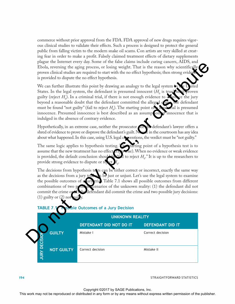
The decisions from hypothesis tests can be either correct or incorrect, exactly the same way as the decisions from a jury trial can be just or unjust. Let’s use the legal system to examine the possible outcomes of a jury trial. Table 7.1 shows all possible outcomes from different combinations of two possible scenarios of the unknown reality: (1) the defendant did not commit the crime or (2) the defendant did commit the crime and two possible jury decisions: (1) guilty or (2) not guilty.
UNKNOWN REALITY
DEFENDANT DID NOT DO IT DEFENDANT DID IT
JURY
DEC
ISIO
N GUILTY Mistake I Correct decision
NOT GUILTY Correct decision Mistake II
TABLE 7.1 Possible Outcomes of a Jury Decision
STRAIGHTFORWARD STATISTICS194
Copyright ©2017 by SAGE Publications, Inc. This work may not be reproduced or distributed in any form or by any means without express written permission of the publisher.
Do not
copy
, pos
t, or d
istrib
ute
The cells inside Table 7.1 represent four different combinations of the unknown reality and the jury decisions. The table clearly shows that there are two correct decisions: (1) when the defendant did not commit the crime and the jury found the defendant not guilty and (2) when the defendant actually committed the crime and the jury found the defendant guilty. There are two different types of mistakes. Mistake I is when the defendant did not commit the crime but the jury found the defendant guilty. Mistake II is when the defendant committed the crime but the jury found the defendant not guilty.
Mistakes incur costs to the society and individuals alike. The presumption of the U.S. society is that Mistake I, putting innocent defendants in prison for crimes they did not commit, is a far worse injustice than Mistake II, letting guilty criminals go free. Although the table shows two types of mistakes and two types of correct decisions, fortunately, they are not a 50–50 split. There are quality control standards in the legal system to make sure that the number of correct decisions outweighs the number of mistakes.
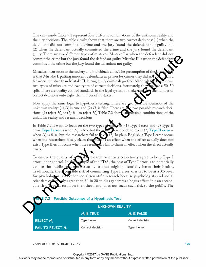
Now apply the same logic to hypothesis testing. There are two possible scenarios of the unknown reality: (1) H
0 is true and (2) H
0 is false. There are also two possible research deci-
sions: (1) reject H0 or (2) fail to reject H
0. Table 7.2 shows all possible combinations of the
unknown reality and research decisions.
In Table 7.2, I want to focus on the two types of mistakes: (1) Type I error and (2) Type II error. Type I error is when H
0 is true but the researchers decide to reject H
0. Type II error is
when H0 is false, but the researchers fail to reject H
0. In plain English, a Type I error occurs
when the researchers falsely claim that there is an effect when the effect actually does not exist. Type II error occurs when the researchers fail to claim an effect when the effect actually exists.
To ensure the quality of scientific research, scientists collectively agree to keep Type I error under control. In the example of the FDA, the cost of Type I error is to potentially expose the public to useless treatments that might potentially harm their health. Traditionally, the acceptable risk of committing Type I error, � is set to be at a .05 level for psychological and other social scientific research because psychologists and social scientists collectively agree that if 1 in 20 studies generates a bogus effect, it is an accept-able risk. Type II error, on the other hand, does not incur such risk to the public. The
UNKNOWN REALITY
H0 IS TRUE H0 IS FALSE
REJECT H0 Type I error Correct decision
FAIL TO REJECT H0Correct decision Type II error
TABLE 7.2 Possible Outcomes of a Hypothesis Test
195CHAPTER 7 • HYPOTHESIS TESTING
Copyright ©2017 by SAGE Publications, Inc. This work may not be reproduced or distributed in any form or by any means without express written permission of the publisher.
Do not
copy
, pos
t, or d
istrib
ute
probability of committing Type II error is called �. Researchers simply fail to claim an effect when an effect actually exists. In such situations, researchers can always start over and conduct more studies later. Sooner or later, someone is going to discover that over-looked effect.
Now, let’s discuss the correct decisions. First, when H0 is true, and the researchers fail to
reject H0, this is a correct decision. The probability of such a correct decision can be calcu-
lated as (1 � �). This probability (1 � �) is also called the confidence level, which will be introduced in Chapter 8. Second, when H
0 is false and the researchers reject H
0, it is again a
correct decision. The probability of such a correct decision is calculated as (1 � �), which is called power. Power is defined as the sensitivity to detect an effect when an effect actually exists. The power of the hypothesis test is the probability of correctly rejecting H
0 when H
0
is false.
Power is an important statistical concept and is influenced by the following three factors:
1. Sample size, n
2. Significance level, �
3. Effect size
Sample size and power are positively correlated. All else being equal, when the sample size is larger, power is bigger. When the sample size is smaller, power is smaller. Large sample size makes a standard error small. When a standard error is small, it is more likely to detect an effect when it actually exists. Sample size is the most influential factor in calcu-lating statistical power because sample size is under the control of researchers. Researchers can plan ahead to figure out how big the sample size needs to be to reach a desirable power level.
Significance level, �, and power are also positively correlated. When � is higher, power is higher. When � is lower, power is lower. The rationale is that when the Type I error is under strict control, the risk of falsely claiming an effect is low; however, the sensitivity to detect an effect is also low. A Type I error is to reject H
0, when H
0 is true. A Type II error is to fail to
reject H0 when H
0 is false. It is obvious that there is a trade-off relationship between the
probability of committing a Type I error, �, and the probability of committing a Type II error, �. As one goes up, the other has to come down. Therefore, when � goes up, researchers decide to increase the risk of Type I error; then � will go down, and (1 � �) will go up. Just remember that � and � move in opposite directions, but � and (1 � �) move in the same direction.
The effect size is positively related with power. The effect size is a standardized measure of the difference between the sample statistic and the hypothesized population parameter in
STRAIGHTFORWARD STATISTICS196
Copyright ©2017 by SAGE Publications, Inc. This work may not be reproduced or distributed in any form or by any means without express written permission of the publisher.
Do not
copy
, pos
t, or d
istrib
ute
units of standard deviation. Such a standardized measure makes it possible to compare results across different studies. A large effect size means that there is a substantial difference between the sample statistic and the hypothe-sized population parameter. When standardized effect size is larger, power is bigger. When stan-dardized effect size is smaller, power is smaller. Therefore, a large effect size makes it easy to detect an effect when the effect actually exists. A small effect size makes it difficult to detect such an effect.
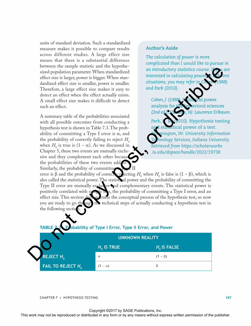
A summary table of the probabilities associated with all possible outcomes from conducting a hypothesis test is shown in Table 7.3. The prob-ability of committing a Type I error is �, and the probability of correctly failing to reject H
0
when H0 is true is (1 – �). As we discussed in
Chapter 5, these two events are mutually exclu-sive and they complement each other because the probabilities of these two events add to 1. Similarly, the probability of committing a Type II error is � and the probability of correctly rejecting H
0 when H
0 is false is (1 – �), which is
also called the statistical power. The statistical power and the probability of committing the Type II error are mutually exclusive and complementary events. The statistical power is positively correlated with sample size, the probability of committing a Type I error, and an effect size. This section demonstrates the conceptual process of the hypothesis test, so now you are ready to go through the technical steps of actually conducting a hypothesis test in the following section.
Author’s Aside
The calculation of power is more complicated than I would like to pursue in an introductory statistics course. If you are interested in calculating power in different situations, you may refer to Cohen (1988) and Park (2010).
Cohen, J. (1988). Statistical power analysis for the behavioral sciences (2nd ed.). Hillsdale, NJ: Lawrence Erlbaum.
Park, H. M. (2010). Hypothesis testing and statistical power of a test. Bloomington, IN: University Information Technology Services, Indiana University. Retrieved from https://scholarworks .iu.edu/dspace/handle/2022/19738
UNKNOWN REALITY
H0 IS TRUE H0 IS FALSE
REJECT H0 � (1 � �)
FAIL TO REJECT H0(1 � �) �
TABLE 7.3 Probability of Type I Error, Type II Error, and Power
197CHAPTER 7 • HYPOTHESIS TESTING
Copyright ©2017 by SAGE Publications, Inc. This work may not be reproduced or distributed in any form or by any means without express written permission of the publisher.
Do not
copy
, pos
t, or d
istrib
ute
The Four-Step Process to Conduct a Hypothesis TestHypothesis testing is a standardized process to test the strength of scientific evidence for a claim about a population. Hypothesis testing involves the following four-step process. All four steps are explained and elaborated in the following sections.
Step 1. Explicitly state the pair of hypotheses.
Step 2. Identify the rejection zone for the hypothesis test.
Step 3. Calculate the test statistic.
Step 4. Make the correct conclusion.
STEP 1. EXPLICITLY STATE THE PAIR OF HYPOTHESES
Hypothesis tests are conducted to test the strength of scientific evidence for a claim about a population. Research purposes are expressed by the pair of hypotheses. H
0 is the “no effect”
(null) hypothesis, and H1 is the research (alternative) hypothesis, which researchers turn to
1. What is the correct definition of Type I error?
a. Reject H0 when H0 is true.
b. Fail to reject H0 when H0 is true.
c. Reject H0 when H0 is false.
d. Fail to reject H0 when H0 is false.
2. What is the correct definition of Type II error?
a. Reject H0 when H0 is true.
b. Fail to reject H0 when H0 is true.
c. Reject H0 when H0 is false.
d. Fail to reject H0 when H0 is false.
3. Which of the following variables is positively correlated with the statistical power?
a. The probability of committing a Type I error, �
b. The sample size, n
c. The effect size
d. All of the above three variables are positively correlated with the statistical power.
Pop Quiz
Answers: 1. a, 2. d, 3. d
STRAIGHTFORWARD STATISTICS198
Copyright ©2017 by SAGE Publications, Inc. This work may not be reproduced or distributed in any form or by any means without express written permission of the publisher.
Do not
copy
, pos
t, or d
istrib
ute
when H0 is rejected by the data. H
1 states the effect that researchers are interested in. Both
hypotheses describe characteristics of the population. Hypothesis tests can be nondirectional or directional. Nondirectional versus directional hypotheses are best illustrated by using an example.
The average IQ score for the general population is � 100. If a researcher wants to compare the average IQ of students in a school district to the population mean, the starting point of this comparison should be explicitly stating the H
0: � 100. It is assumed that the average IQ
score of students in this school district is the same as the population. Then, the alternative hypothesis needs to be stated. Depending on the nature of the comparison, the researchers may use nondirectional hypothesis testing or directional hypothesis testing. Nondirectional hypothesis testing is only interested in whether the sample could come from a population with the hypothesized mean or not, so the alternative hypothesis is H
1: � 100. A nondirec-
tional hypothesis test is called a two-tailed test.
Directional hypothesis testing, on the other hand, is interested in a particular direction, so the alternative hypothesis could be expressed as either higher or lower than the population parameter, H
1: � � 100 or H
1: � � 100. A directional hypothesis test is also called a one-tailed
test. Under a one-tailed test, the alternative hypothesis is stated with a direction such as a right-tailed test or a left-tailed test. Which of these tests to use depends on whether the problem statement contains clear direction with key words such as “higher,” “increasing,” “improving,” “lower,” “decreasing,” or “deteriorating.” When the problem statement contains these key words for a particular direction, one-tailed tests are appropriate. To complete the example of the IQ score, here is a list of hypotheses in all possible tests.
Two-tailed test: H0: μ 100
H1: μ 100
Right-tailed test: H0: μ 100
H1: μ � 100
Left-tailed test: H0: μ 100
H1: μ � 100
This list illustrates that H0 is the “no effect” hypothesis. It states that the average IQ score of
students in the school district is the same as the population parameter. Please note that the “” sign is always in H
0, the null hypothesis.
The alternative hypothesis, H1, is the hypothesis that researchers turn to when H
0 is rejected. It
states that there is some kind of difference between the average IQ scores of students in the school district and the population mean. The nature of the difference depends on whether the test is a two-tailed test, a right-tailed test, or a left-tailed test. H
1 in a two-tailed test states that the
average IQ score of students in the school district is not the same as the hypothesized population
199CHAPTER 7 • HYPOTHESIS TESTING
Copyright ©2017 by SAGE Publications, Inc. This work may not be reproduced or distributed in any form or by any means without express written permission of the publisher.
Do not
copy
, pos
t, or d
istrib
ute

mean. H1 in a right-tailed test states that the average IQ score of students in the school district is
higher than the hypothesized population mean. H1 in a left-tailed test states that the average IQ
score of students in the school district is lower than the hypothesized population mean.
You might have seen other textbooks list one-tailed tests as H0: � 100 and H
1: � � 100 in a
right-tailed test or H0: � � 100 and H
1: � � 100 in a left-tailed test, so that all possible out-
comes are included in the pair of hypotheses. These kinds of expressions are regarded as out-dated. In this book, for the sake of simplicity and clarity, all null hypotheses remain with “” sign only. It is implied that the single direction sign (� or �) opposite to the H
1 is included in
the H0. For example, a swimming coach is testing the effectiveness of a particular training
routine. The purpose of the training routine is to drop swimmers’ times and make them swim faster. Therefore, the hypothesis test is set up as a left-tailed test. If the swimmers’ times do not change, then we have to conclude that the training routine has no effect (i.e., we fail to reject H
0). Obviously, if the swimmers’ times get slower due to the training routine, clearly not the
effect intended by the coach, we have to conclude that the training routine has no effect.
STEP 2. IDENTIFY THE REJECTION ZONE FOR THE HYPOTHESIS TEST
As discussed in the previous section, social scientists collectively agree that Type I errors need to be kept under control to protect the general public from falsely claimed effects. The prob-ability to commit a Type I error is � and is the key to establishing the decision rules for the hypothesis test. Therefore, � is also called the significance level. Different � levels may be assigned according to the nature of the research. In a research project with strong theoretical reasoning behind it, or in a project with many similar studies being conducted repeatedly and resulting in consistent findings, a strict standard may apply, such as � .01. In contrast, in a research project of an exploratory nature, without much if any theoretical reasoning to back it up, a weak standard may suffice, such as � .10. Usually for research in social sciences, the default level is � .05.
The significance level helps identify the rejection zone. The rejection zone is bounded by the critical value of a statistic. Once the rejection zone is set, decision rules can be clearly stated. If any calculated test statistic falls in the rejection zone, the decision is to reject H
0. Otherwise,
if the test statistic does not fall in the rejection zone, we fail to reject H0. The term fail to reject
H0 is a double negative and seems cumbersome. I will explain in more detail why “fail to
reject H0” is preferred to “accept H
0” in Step 4, which is to make the correct conclusion.
Let’s continue the previous IQ example to identify the rejection zones assuming � .05. First, we use � .05 to identify the rejection zone for a two-tailed test.
Two-tailed test: H0: μ 100
H1: μ 100
Rejection zone: Z Z> α /2
STRAIGHTFORWARD STATISTICS200
Copyright ©2017 by SAGE Publications, Inc. This work may not be reproduced or distributed in any form or by any means without express written permission of the publisher.
Do not
copy
, pos
t, or d
istrib
ute
Next, we use � .05 to identify the rejection zone for a right-tailed test.
Right-tailed test: H0: � 100
H1: � � 100
Rejection zone: Z � Z�
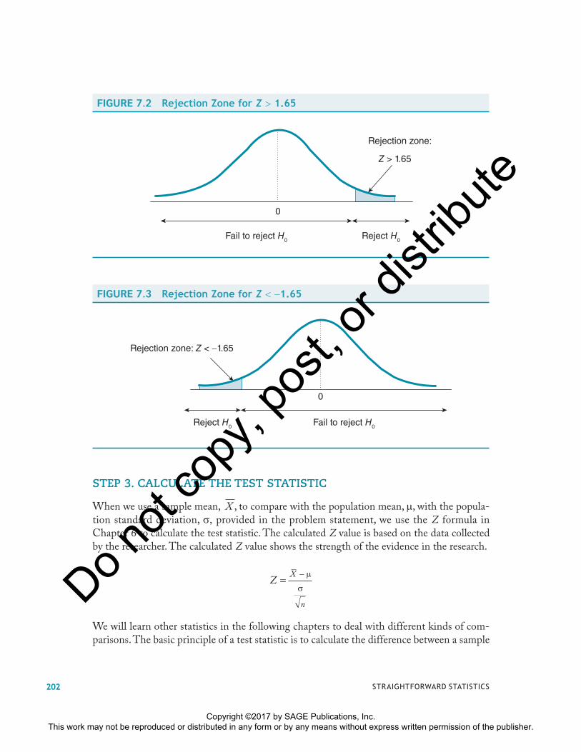
In a right-tailed test, the significance level, �, is solely in the right tail. Assuming � .05, the probability of the right tail is .05. According to the Z table, when the tail probability is .05, the critical value of Z is between 1.64 and 1.65. I prefer to use the more conservative (i.e., a higher standard and more difficult to reach) standard, so I pick the value 1.65. Therefore, the best way to express the rejection zone for a right-tailed test is Z � 1.65, as shown in Figure 7.2.
Next, we use � .05 to identify the rejection zone for a left-tailed test.
Left-tailed test: H0: � 100
H1: � � 100
Rejection zone: Z � �Z�
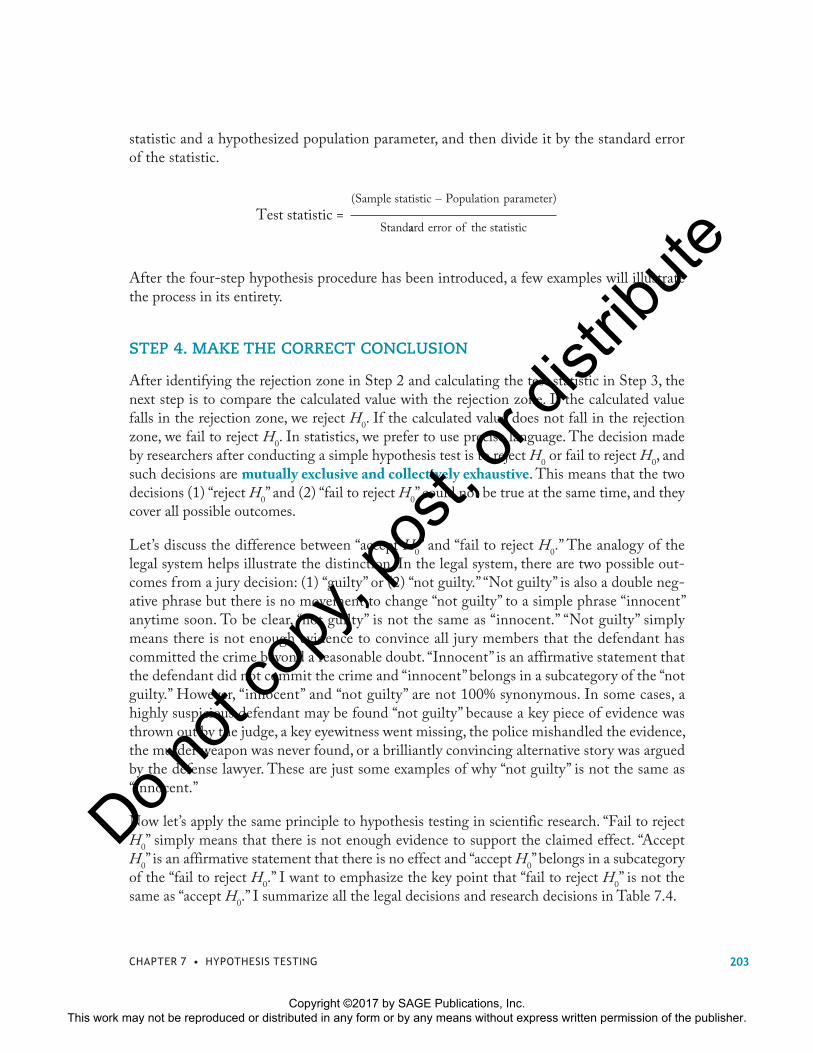
The rejection zone for a left tailed test is Z � �1.65, as shown in Figure 7.3.
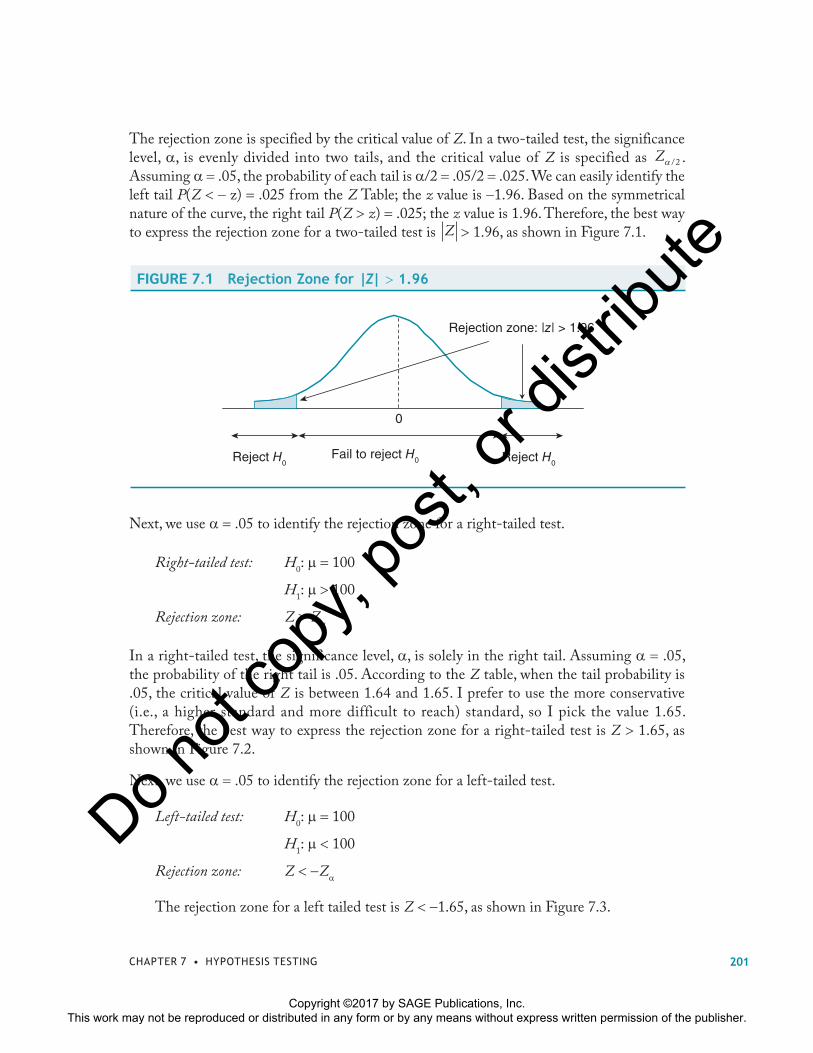
The rejection zone is specified by the critical value of Z. In a two-tailed test, the significance level, �, is evenly divided into two tails, and the critical value of Z is specified as Z� /2 . Assuming � .05, the probability of each tail is �/2 .05/2 .025. We can easily identify the left tail P(Z � � z) .025 from the Z Table; the z value is �1.96. Based on the symmetrical nature of the curve, the right tail P(Z � z) .025; the z value is 1.96. Therefore, the best way to express the rejection zone for a two-tailed test is Z � 1.96, as shown in Figure 7.1.
FIGURE 7.1 Rejection Zone for |Z| � 1.96
Rejection zone: |z| > 1.96
0
Reject H0Fail to reject H0Reject H0
201CHAPTER 7 • HYPOTHESIS TESTING
Copyright ©2017 by SAGE Publications, Inc. This work may not be reproduced or distributed in any form or by any means without express written permission of the publisher.
Do not
copy
, pos
t, or d
istrib
ute
STEP 3. CALCULATE THE TEST STATISTIC
When we use a sample mean, X , to compare with the population mean, �, with the popula-tion standard deviation, �� provided in the problem statement, we use the Z formula in Chapter 6 to calculate the test statistic. The calculated Z value is based on the data collected by the researcher. The calculated Z value shows the strength of the evidence in the research.
ZX
n
=− μ
σ
We will learn other statistics in the following chapters to deal with different kinds of com-parisons. The basic principle of a test statistic is to calculate the difference between a sample
FIGURE 7.2 Rejection Zone for Z � 1.65
Fail to reject H0 Reject H0
0
Rejection zone:
Z > 1.65
FIGURE 7.3 Rejection Zone for Z � �1.65
Rejection zone: Z < −1.65
Reject H0 Fail to reject H0
0
STRAIGHTFORWARD STATISTICS202
Copyright ©2017 by SAGE Publications, Inc. This work may not be reproduced or distributed in any form or by any means without express written permission of the publisher.
Do not
copy
, pos
t, or d
istrib
ute
statistic and a hypothesized population parameter, and then divide it by the standard error of the statistic.
Test statistic = (Sample statistic Population parameter)
Stand
�
aard error of the statistic
After the four-step hypothesis procedure has been introduced, a few examples will illustrate the process in its entirety.
STEP 4. MAKE THE CORRECT CONCLUSION
After identifying the rejection zone in Step 2 and calculating the test statistic in Step 3, the next step is to compare the calculated value with the rejection zone. If the calculated value falls in the rejection zone, we reject H
0. If the calculated value does not fall in the rejection
zone, we fail to reject H0. In statistics, we prefer to use precise language. The decision made
by researchers after conducting a simple hypothesis test is to reject H0 or fail to reject H
0, and
such decisions are mutually exclusive and collectively exhaustive. This means that the two decisions (1) “reject H
0” and (2) “fail to reject H
0” could not be true at the same time, and they
cover all possible outcomes.
Let’s discuss the difference between “accept H0” and “fail to reject H
0.” The analogy of the
legal system helps illustrate the distinction. In the legal system, there are two possible out-comes from a jury decision: (1) “guilty” or (2) “not guilty.” “Not guilty” is also a double neg-ative phrase but there is no movement to change “not guilty” to a simple phrase “innocent” anytime soon. To be clear, “not guilty” is not the same as “innocent.” “Not guilty” simply means there is not enough evidence to convince all jury members that the defendant has committed the crime beyond a reasonable doubt. “Innocent” is an affirmative statement that the defendant did not commit the crime and “innocent” belongs in a subcategory of the “not guilty.” However, “innocent” and “not guilty” are not 100% synonymous. In some cases, a highly suspicious defendant may be found “not guilty” because a key piece of evidence was thrown out by the judge, a key eyewitness went missing, the police mishandled the evidence, the murder weapon was never found, or a brilliantly convincing alternative story was argued by the defense lawyer. These are just some examples of why “not guilty” is not the same as “innocent.”
Now let’s apply the same principle to hypothesis testing in scientific research. “Fail to reject H
0” simply means that there is not enough evidence to support the claimed effect. “Accept
H0” is an affirmative statement that there is no effect and “accept H
0” belongs in a subcategory
of the “fail to reject H0.” I want to emphasize the key point that “fail to reject H
0” is not the
same as “accept H0.” I summarize all the legal decisions and research decisions in Table 7.4.
203CHAPTER 7 • HYPOTHESIS TESTING
Copyright ©2017 by SAGE Publications, Inc. This work may not be reproduced or distributed in any form or by any means without express written permission of the publisher.
Do not
copy
, pos
t, or d
istrib
ute
Here is a real-life example to illustrate why this seemingly trivial distinction might have major consequences. A few years ago, I attended a research presentation made by a job candidate seeking a tenure-track position at a university. The candidate presented his research to the faculty members in the department where the hiring decision was going to be made. The can-didate’s research topic was on spatial orientation. According to the previous literature, spatial orientation is an ability that consistently shows significant gender differences. After his pre-sentation, I asked, “Did you find any gender difference in your study on spatial orientation?” He answered, “There were no gender differences in my study.” The answer would have been much better if he said, “There was not enough evidence to support the claim that gender dif-ferences existed in my study.” “There were no gender differences in my study” is the “accept H
0” answer. “There was not enough evidence to support the claim that gender differences
exist” is the “fail to reject H0” answer. The fail to reject H
0 answer is logically and technically
superior to the accept H0 answer. The job candidate’s research was not focused on gender dif-
ferences, and the research design was not conducive to show whether they existed or not. There simply was not enough evidence on gender differences in his study. Being able to answer questions correctly during a job interview might have a big impact on the hiring decision.
Let’s move on to more specific examples of how the four-step hypothesis test works in action.
EXAMPLES OF THE FOUR-STEP HYPOTHESIS TEST IN ACTION
The four-step hypothesis test is a standard scientific approach to test the significance of the empirical evidence on a claim about a population. Such a four-step hypothesis testing process will be useful not only in this chapter but also in all of the later chapters. Let’s go through the four-step process by using a couple of examples.
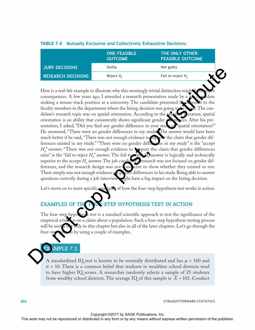
ONE FEASIBLE OUTCOME
THE ONLY OTHER FEASIBLE OUTCOME
JURY DECISIONS Guilty Not guilty
RESEARCH DECISIONS Reject H0 Fail to reject H0
TABLE 7.4 Mutually Exclusive and Collectively Exhaustive Decisions
A standardized IQ test is known to be normally distributed and has � 100 and � 10. There is a common belief that students in wealthier school districts tend to have higher IQ scores. A researcher randomly selects a sample of 25 students from wealthy school districts. The average IQ of this sample is X 103. Conduct
EXAMPLE 7.1
STRAIGHTFORWARD STATISTICS204
Copyright ©2017 by SAGE Publications, Inc. This work may not be reproduced or distributed in any form or by any means without express written permission of the publisher.
Do not
copy
, pos
t, or d
istrib
ute
a test to verify if the average IQ score for students from wealthy districts is higher than 100, assuming � .05.
We are going to use the four-step hypothesis testing process to answer this question.
Step 1. State the pair of hypotheses.
Based on the problem statement “If the average IQ score for students from wealthy districts is higher than 100,” the problem indicates a directional hypothe-sis. The key word “higher IQ scores” indicates a right-tailed test. The alternative hypothesis, H
1, is � � 100. Then H
0 covers the equal sign, � 100. It is important
to point out that the research interest is to compare the average IQ score of stu-dents from wealthy districts to the general population mean. The research interest is not to compare the sample mean of the 25 students to the general population mean. Thus, the hypotheses must be phrased to describe the “research population,” which refers to all students in wealthy districts.
H0: � 100
H1: � � 100
Step 2. Identify the rejection zone for the hypothesis test.
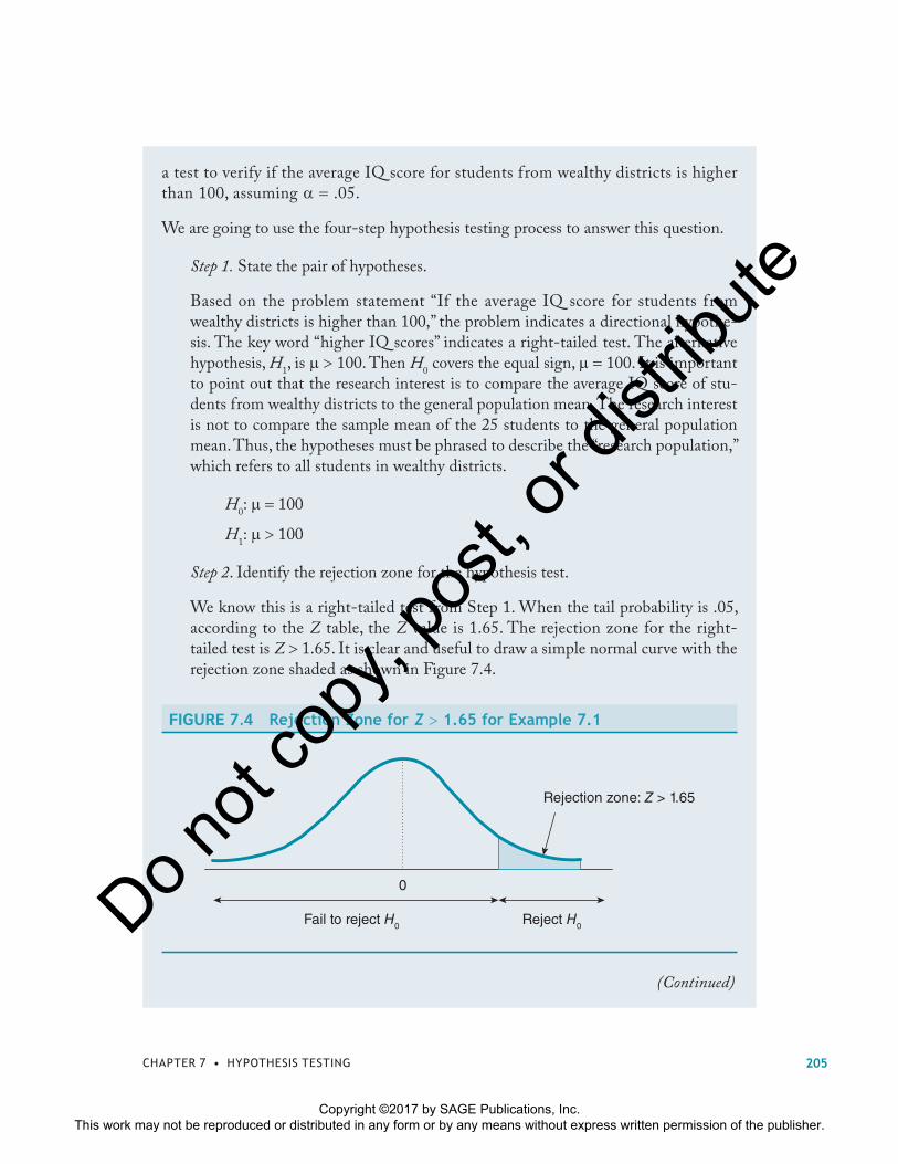
We know this is a right-tailed test from Step 1. When the tail probability is .05, according to the Z table, the Z value is 1.65. The rejection zone for the right-tailed test is Z � 1.65. It is clear and useful to draw a simple normal curve with the rejection zone shaded as shown in Figure 7.4.
FIGURE 7.4 Rejection Zone for Z � 1.65 for Example 7.1
0
Fail to reject H0 Reject H0
Rejection zone: Z > 1.65
(Continued)
205CHAPTER 7 • HYPOTHESIS TESTING
Copyright ©2017 by SAGE Publications, Inc. This work may not be reproduced or distributed in any form or by any means without express written permission of the publisher.
Do not
copy
, pos
t, or d
istrib
ute
Statistics are widely available in different situations. Besides IQ scores or standardized test scores, life expectancy is a commonly available statistic locally, nationally, and inter-nationally. Let’s use life expectancy as an example to conduct a hypothesis test in the next example.
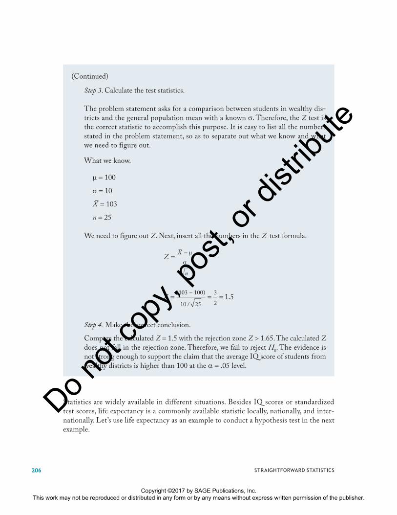
Step 3. Calculate the test statistics.
The problem statement asks for a comparison between students in wealthy dis-tricts and the general population mean with a known �. Therefore, the Z test is the correct statistic to accomplish this purpose. It is easy to list all the numbers stated in the problem statement, so as to separate out what we know and what we need to figure out.
What we know.
� 100
� 10
X 103
n 25
We need to figure out Z. Next, insert all the numbers in the Z-test formula.
ZX
n
=− μ
σ
Z = = =−( )
/.
103 100
10 25
3
21 5
Step 4. Make the correct conclusion.
Compare the calculated Z 1.5 with the rejection zone Z � 1.65. The calculated Z does not fall in the rejection zone. Therefore, we fail to reject H
0. The evidence is
not strong enough to support the claim that the average IQ score of students from wealthy districts is higher than 100 at the � .05 level.
(Continued)
STRAIGHTFORWARD STATISTICS206
Copyright ©2017 by SAGE Publications, Inc. This work may not be reproduced or distributed in any form or by any means without express written permission of the publisher.
Do not
copy
, pos
t, or d
istrib
ute
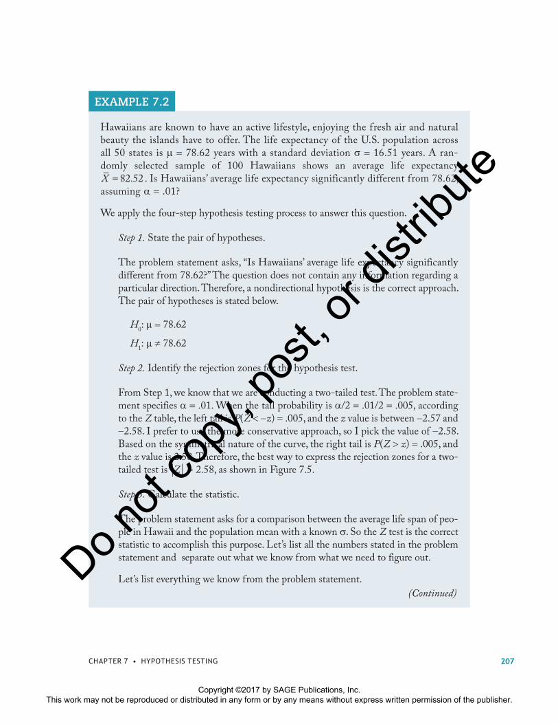
Hawaiians are known to have an active lifestyle, enjoying the fresh air and natural beauty the islands have to offer. The life expectancy of the U.S. population across all 50 states is � 78.62 years with a standard deviation � 16.51 years. A ran-domly selected sample of 100 Hawaiians shows an average life expectancy X 82 52. . Is Hawaiians’ average life expectancy significantly different from 78.62, assuming � .01?
We apply the four-step hypothesis testing process to answer this question.
Step 1. State the pair of hypotheses.
The problem statement asks, “Is Hawaiians’ average life expectancy significantly different from 78.62?” The question does not contain any information regarding a particular direction. Therefore, a nondirectional hypothesis is the correct approach. The pair of hypotheses is stated below.
H0: � 78.62
H1: � 78.62
Step 2. Identify the rejection zones for the hypothesis test.
From Step 1, we know that we are conducting a two-tailed test. The problem state-ment specifies � .01. When the tail probability is �/2 .01/2 .005, according to the Z table, the left tail is P(Z � �z) .005, and the z value is between �2.57 and �2.58. I prefer to use the more conservative approach, so I pick the value of �2.58. Based on the symmetrical nature of the curve, the right tail is P(Z � z) .005, and the z value is 2.58. Therefore, the best way to express the rejection zones for a two-tailed test is Z � 2.58, as shown in Figure 7.5.
Step 3. Calculate the statistic.
The problem statement asks for a comparison between the average life span of peo-ple in Hawaii and the population mean with a known �. So the Z test is the correct statistic to accomplish this purpose. Let’s list all the numbers stated in the problem statement and separate out what we know from what we need to figure out.
Let’s list everything we know from the problem statement.
EXAMPLE 7.2
(Continued)
207CHAPTER 7 • HYPOTHESIS TESTING
Copyright ©2017 by SAGE Publications, Inc. This work may not be reproduced or distributed in any form or by any means without express written permission of the publisher.
Do not
copy
, pos
t, or d
istrib
ute
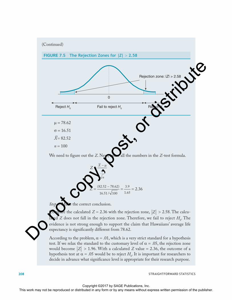
� 78.62
� 16.51
X 82.52
n 100
We need to figure out the Z. Next, insert all the numbers in the Z-test formula.
ZX
n
=− μ
σ
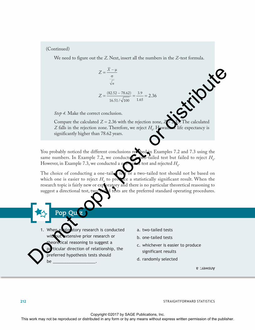
Z = = =−( . . )
. /
.
..
82 52 78 62
16 51 100
3 9
1 652 36
Step 4. Make the correct conclusion.
Compare the calculated Z 2.36 with the rejection zone, Z � 2.58. The calcu-
lated Z does not fall in the rejection zone. Therefore, we fail to reject H0. The
evidence is not strong enough to support the claim that Hawaiians’ average life expectancy is significantly different from 78.62.
According to the problem, � .01, which is a very strict standard for a hypothesis test. If we relax the standard to the customary level of � .05, the rejection zone would become Z � 1.96. With a calculated Z value 2.36, the outcome of a hypothesis test at � .05 would be to reject H
0. It is important for researchers to
decide in advance what significance level is appropriate for their research purpose.
FIGURE 7.5 The Rejection Zones for |Z| � 2.58
Rejection zone: |Z| > 2.58
Reject H0 Reject H0Fail to reject H0
0
(Continued)
STRAIGHTFORWARD STATISTICS208
Copyright ©2017 by SAGE Publications, Inc. This work may not be reproduced or distributed in any form or by any means without express written permission of the publisher.
Do not
copy
, pos
t, or d
istrib
ute
Directional Versus Nondirectional Hypothesis TestingDirectional hypothesis tests versus nondirectional hypothesis tests is a topic that needs to be discussed in detail. The most noticeable difference between one-tailed tests and two-tailed
After going through a couple of examples, it is clear that the four-step hypothesis testing procedure is a standardized scientific process to test the strength of the empirical evidence on a claim about the population. Let’s recap that process.
Step 1. Explicitly state the pair of hypotheses. This means to declare the purpose of the hypothesis test and identify whether it is a directional test or a nondirectional test.
Step 2. Identify the rejection zone for the hypothesis test. Based on the predetermined significance level, the rejection zone can be specified by the critical value of Z. The rejection zone serves as a criterion for decision making on the outcomes of the hypothesis test.
Step 3. Calculate the test statistic. Many different statistical tests will be discussed throughout this book. So far, we have only covered the Z test.
Step 4. Make the correct conclusion. The research conclusion is made by comparing the calculated value of the test statistic and the rejection zone. If the calculated test statistic is within the rejection zone, we reject H
0. When we reject H
0, it means that the evidence
is strong enough to claim an effect. If the calculated test statistic is not within the rejec-tion zone, we fail to reject H
0. When we fail to reject H
0, it means that the evidence is not
strong enough to support a claim of an effect.
1. What values are needed to figure out the rejection zones for Z tests?
a. The significance level, �
b. One-tailed test or two-tailed test
c. Sample size
d. Both (a) and (b)
e. All of the above
2. For a two-tailed Z test with � .10, the critical values that set the boundaries for the rejection zones are
a. Z � 1.65
b. Z � 1.96
c. Z � 1.65
d. Z �1.96
Pop Quiz
Answers: 1. d, 2. c
209CHAPTER 7 • HYPOTHESIS TESTING
Copyright ©2017 by SAGE Publications, Inc. This work may not be reproduced or distributed in any form or by any means without express written permission of the publisher.
Do not
copy
, pos
t, or d
istrib
ute
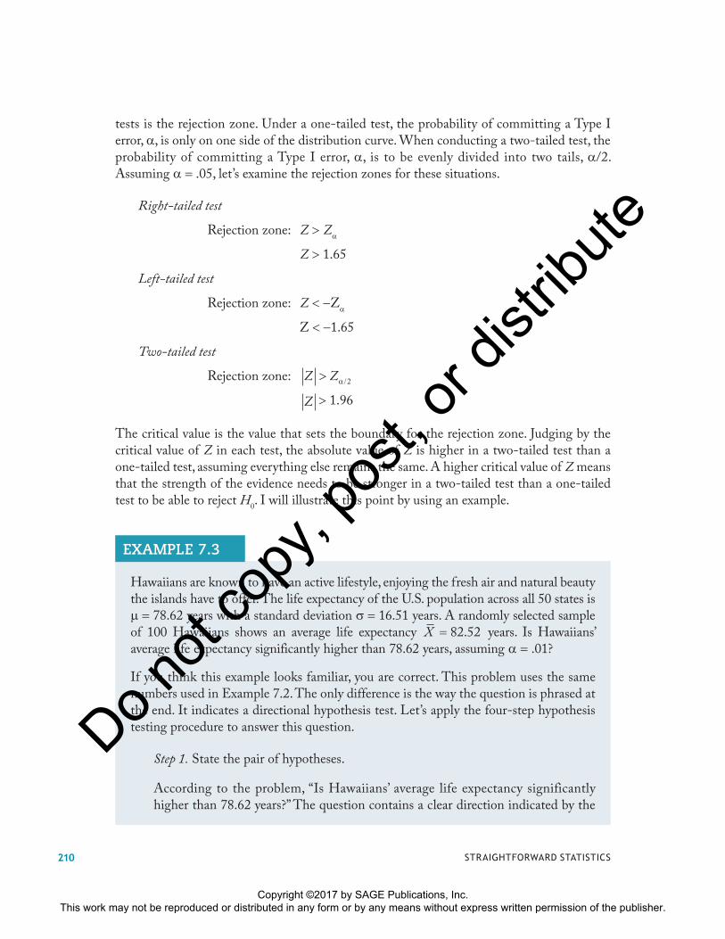
tests is the rejection zone. Under a one-tailed test, the probability of committing a Type I error, �, is only on one side of the distribution curve. When conducting a two-tailed test, the probability of committing a Type I error, �, is to be evenly divided into two tails, �/2. Assuming � .05, let’s examine the rejection zones for these situations.
Right-tailed test
Rejection zone: Z � Z�
Z � 1.65
Left-tailed test
Rejection zone: Z � �Z�
Z � �1.65
Two-tailed test
Rejection zone: Z Z> α/2
Z � 1.96
The critical value is the value that sets the boundary for the rejection zone. Judging by the critical value of Z in each test, the absolute value of Z is higher in a two-tailed test than a one-tailed test, assuming everything else remains the same. A higher critical value of Z means that the strength of the evidence needs to be stronger in a two-tailed test than a one-tailed test to be able to reject H
0. I will illustrate this point by using an example.
Hawaiians are known to have an active lifestyle, enjoying the fresh air and natural beauty the islands have to offer. The life expectancy of the U.S. population across all 50 states is � 78.62 years with a standard deviation � 16.51 years. A randomly selected sample of 100 Hawaiians shows an average life expectancy X 82 52. years. Is Hawaiians’ average life expectancy significantly higher than 78.62 years, assuming � .01?
If you think this example looks familiar, you are correct. This problem uses the same numbers used in Example 7.2. The only difference is the way the question is phrased at the end. It indicates a directional hypothesis test. Let’s apply the four-step hypothesis testing procedure to answer this question.
Step 1. State the pair of hypotheses.
According to the problem, “Is Hawaiians’ average life expectancy significantly higher than 78.62 years?” The question contains a clear direction indicated by the
EXAMPLE 7.3
STRAIGHTFORWARD STATISTICS210
Copyright ©2017 by SAGE Publications, Inc. This work may not be reproduced or distributed in any form or by any means without express written permission of the publisher.
Do not
copy
, pos
t, or d
istrib
ute
key word “higher.” Therefore, a directional hypothesis, in this case, a right-tailed test, is the correct approach. The pair of hypotheses is stated below.
H0: � 78.62
H1: � � 78.62
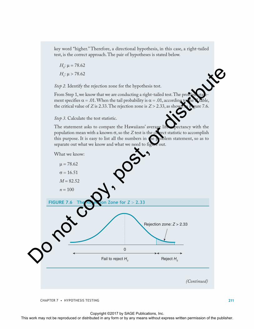
Step 2. Identify the rejection zone for the hypothesis test.
From Step 1, we know that we are conducting a right-tailed test. The problem state-ment specifies � .01. When the tail probability is � .01, according to the Z table, the critical value of Z is 2.33. The rejection zone is Z � 2.33, as shown in Figure 7.6.
Step 3. Calculate the test statistic.
The statement asks to compare the Hawaiians’ average life expectancy with the population mean with a known �, so the Z test is the correct statistic to accomplish this purpose. It is easy to list all the numbers in the problem statement, so as to separate out what we know and what we need to figure out.
What we know:
� 78.62
� 16.51
M 82.52
n 100
FIGURE 7.6 The Rejection Zone for Z � 2.33
0
Fail to reject H0 Reject H0
Rejection zone: Z > 2.33
(Continued)
211CHAPTER 7 • HYPOTHESIS TESTING
Copyright ©2017 by SAGE Publications, Inc. This work may not be reproduced or distributed in any form or by any means without express written permission of the publisher.
Do not
copy
, pos
t, or d
istrib
ute
1. When exploratory research is conducted without extensive prior research or theoretical reasoning to suggest a particular direction of relationship, the preferred hypothesis tests should be ___________________.
a. two-tailed tests
b. one-tailed tests
c. whichever is easier to produce significant results
d. randomly selected
Pop Quiz
Answer: aWe need to figure out the Z. Next, insert all the numbers in the Z-test formula.
ZX
n
=− μ
σ
Z = = =−( . . )
. /
.
..
82 52 78 62
16 51 100
3 9
1 652 36
Step 4. Make the correct conclusion.
Compare the calculated Z 2.36 with the rejection zone, Z � 2.33. The calculated Z falls in the rejection zone. Therefore, we reject H
0. Hawaiians’ life expectancy is
significantly higher than 78.62 years.
You probably noticed the different conclusions reached in Examples 7.2 and 7.3 using the same numbers. In Example 7.2, we conducted a two-tailed test but failed to reject H
0.
However, in Example 7.3, we conducted a one-tailed test and rejected H0.
The choice of conducting a one-tailed test or a two-tailed test should not be based on which one is easier to reject H
0 to produce a statistically significant result. When the
research topic is fairly new or exploratory and there is no particular theoretical reasoning to suggest a directional test, two-tailed tests are the preferred standard operating procedures.
(Continued)
STRAIGHTFORWARD STATISTICS212
Copyright ©2017 by SAGE Publications, Inc. This work may not be reproduced or distributed in any form or by any means without express written permission of the publisher.
Do not
copy
, pos
t, or d
istrib
ute
One-tailed tests are usually reserved for research topics that have been studied repeatedly, for which consistent directional results have been obtained, or in which theoretical reasoning strongly suggests directional outcomes.
Exercise Problems 1. According to the ACT Profile Report-National, the ACT composite scores are
normally distributed with � 21.0 and � 5.4. Many charter schools receive fund-ing from the state government without providing accountability measures as required by the public schools. A sample of 36 high school seniors is randomly selected from charter schools. Their average ACT composite score is 19.8. Is the average ACT composite score of seniors from charter schools lower than 21.0, assuming � .10?
2. Assume that the heights of a population of adults form a normal distribution with a mean � 69 inches and a standard deviation � 6 inches. A village is known to have tall people. A researcher randomly selects a group of 25 people from this village, and their average height is 5 feet 11 inches. Is the average height of people from this vil-lage more than 69 inches, assuming � .05?
3. A car manufacturer claims that a new model Q has an average fuel efficiency � 35 miles per gallon on the highway, and a standard deviation � 5. The American Automobile Association randomly selects 16 new Qs and measures their fuel effi-ciency at 33 miles per gallon. Is the car manufacturer truthful in advertising Q’s fuel efficiency as being 35 miles per gallon, assuming � .10?
Solutions
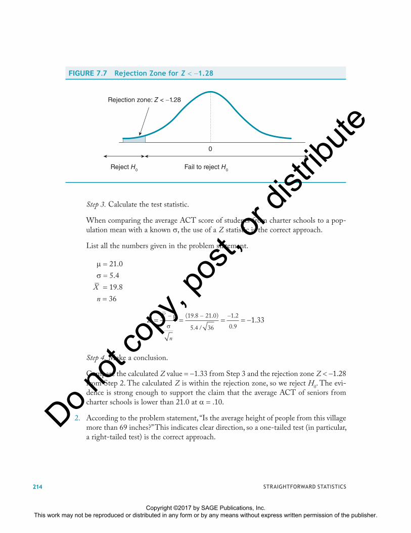
1. The problem statement is whether the average ACT composite score of seniors from charter schools is lower than 21.0. “Lower” is a key word for direction; therefore, a left-tailed test is appropriate.
Step 1. State the pair of hypotheses.
Left-tailed test: H0: � 21.0
H1: � � 21.0
Step 2. Identify the rejection zone.
For a left-tailed test with � .10, the critical value of Z is 1.28. The rejection zone is Z � �1.28, as shown in Figure 7.7.
213CHAPTER 7 • HYPOTHESIS TESTING
Copyright ©2017 by SAGE Publications, Inc. This work may not be reproduced or distributed in any form or by any means without express written permission of the publisher.
Do not
copy
, pos
t, or d
istrib
ute
Step 3. Calculate the test statistic.
When comparing the average ACT score of students from charter schools to a pop-ulation mean with a known �, the use of a Z statistic is the correct approach.
List all the numbers given in the problem statement.
� � 21.0
� � 5.4
X 19.8
n 36
ZX
n
= = = = −− − −μ
σ
( . . )
. /
.
..
19 8 21 0
5 4 36
1 2
0 91 33
Step 4. Make a conclusion.
Compare the calculated Z value �1.33 from Step 3 and the rejection zone Z � �1.28 from Step 2. The calculated Z is within the rejection zone, so we reject H
0. The evi-
dence is strong enough to support the claim that the average ACT of seniors from charter schools is lower than 21.0 at � .10.
2. According to the problem statement, “Is the average height of people from this village more than 69 inches?” This indicates clear direction, so a one-tailed test (in particular, a right-tailed test) is the correct approach.
FIGURE 7.7 Rejection Zone for Z � �1.28
Rejection zone: Z < −1.28
0
Reject H0 Fail to reject H0
STRAIGHTFORWARD STATISTICS214
Copyright ©2017 by SAGE Publications, Inc. This work may not be reproduced or distributed in any form or by any means without express written permission of the publisher.
Do not
copy
, pos
t, or d
istrib
ute
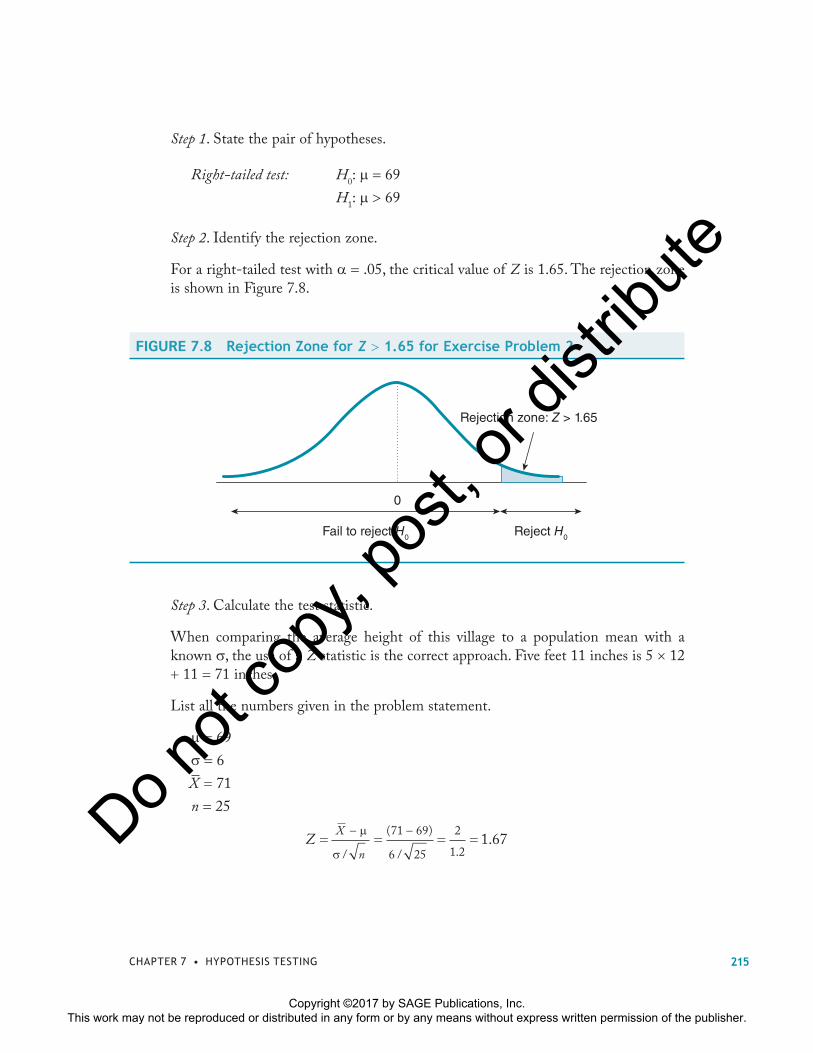
Step 1. State the pair of hypotheses.
Right-tailed test: H0: � 69
H1: � � 69
Step 2. Identify the rejection zone.
For a right-tailed test with � .05, the critical value of Z is 1.65. The rejection zone is shown in Figure 7.8.
FIGURE 7.8 Rejection Zone for Z � 1.65 for Exercise Problem 2
0
Fail to reject H0 Reject H0
Rejection zone: Z > 1.65
Step 3. Calculate the test statistic.
When comparing the average height of this village to a population mean with a known �, the use of a Z statistic is the correct approach. Five feet 11 inches is 5 � 12 � 11 71 inches.
List all the numbers given in the problem statement.
� � 69
� � 6
X 71
n 25
ZX
n= = = =
− −μ
σ /
( )
/ ..
71 69
6 25
2
1 21 67
215CHAPTER 7 • HYPOTHESIS TESTING
Copyright ©2017 by SAGE Publications, Inc. This work may not be reproduced or distributed in any form or by any means without express written permission of the publisher.
Do not
copy
, pos
t, or d
istrib
ute
Step 4. Make the correct conclusion.
Compare the calculated Z value 1.67 from Step 3 and the rejection zone Z � 1.65 from Step 2. The calculated Z falls in the rejection zone, so we reject H
0. The evidence
is strong enough to support the claim that the average height of people in this village is more than 69 inches.
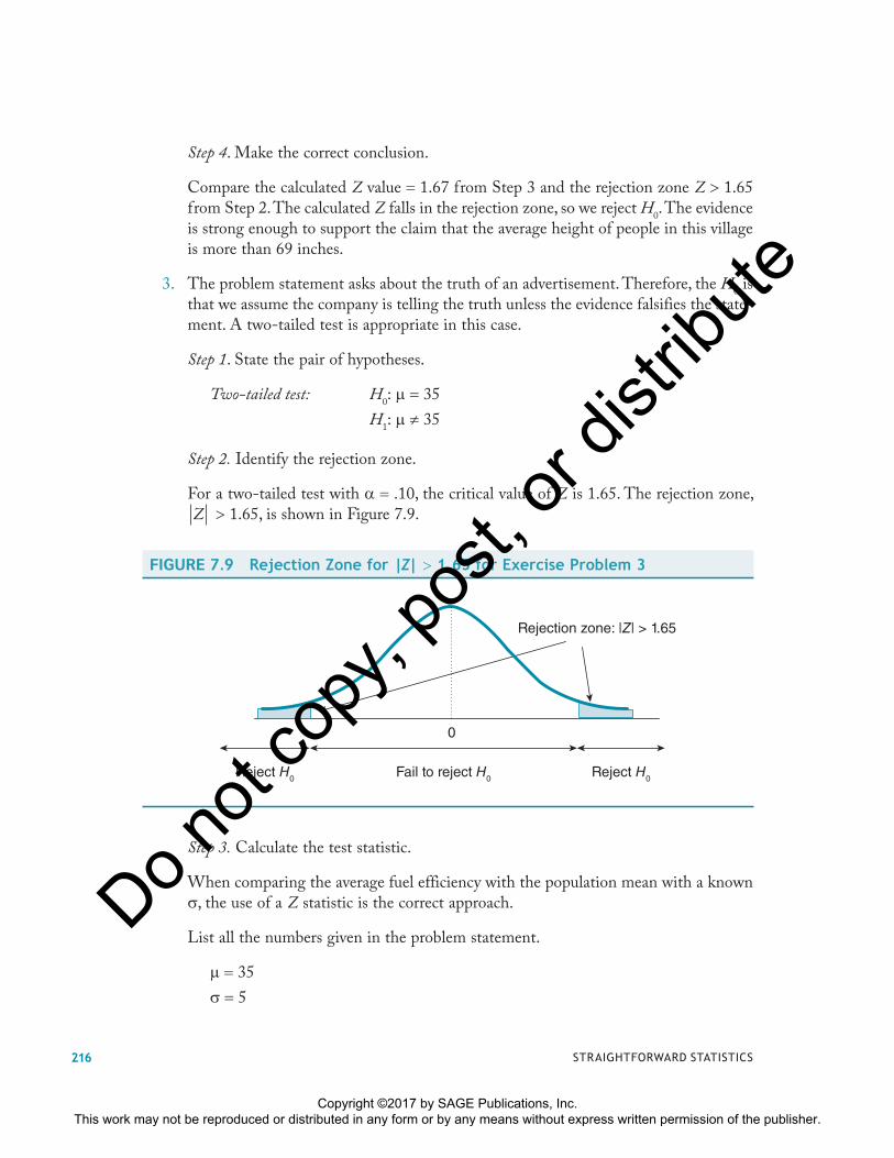
3. The problem statement asks about the truth of an advertisement. Therefore, the H0 is
that we assume the company is telling the truth unless the evidence falsifies the state-ment. A two-tailed test is appropriate in this case.
Step 1. State the pair of hypotheses.
Two-tailed test: H0: � 35
H1: � 35
Step 2. Identify the rejection zone.
For a two-tailed test with � .10, the critical value of Z is 1.65. The rejection zone, Z � 1.65, is shown in Figure 7.9.
FIGURE 7.9 Rejection Zone for |Z| � 1.65 for Exercise Problem 3
Reject H0 Reject H0Fail to reject H0
Rejection zone: |Z| > 1.65
0
Step 3. Calculate the test statistic.
When comparing the average fuel efficiency with the population mean with a known �, the use of a Z statistic is the correct approach.
List all the numbers given in the problem statement.
� � 35
� � 5
STRAIGHTFORWARD STATISTICS216
Copyright ©2017 by SAGE Publications, Inc. This work may not be reproduced or distributed in any form or by any means without express written permission of the publisher.
Do not
copy
, pos
t, or d
istrib
ute
X 33
n 16
ZX
n= = = = −
− − −μ
σ /
( )
/ ..
33 35
5 16
2
1 251 6
Step 4. Make a conclusion.
Compare the calculated Z value �1.6 from Step 3 and the rejection zone Z � 1.65 from Step 2. The calculated Z does not fall in the rejection zone, so we fail to reject H
0. The evidence is not strong enough to reject H
0. The evidence is not strong enough
to support the claim that the company is not truthful in its advertisement.
Sharpen your skills with SAGE edge!
Visit edge.sagepub.com/bowen for mobile-friendly quizzes, flashcards, videos, and more!
What You Learned
Hypothesis testing involves problem-solving skills. At the outset, one must understand the problem statement to determine if any key word indicates a clear direction of the test. If so, a one-tailed test is the correct approach. If not, a two-tailed test is the correct solution. Due to the limited statistical topics covered so far, only the Z test is used to illustrate hypothesis testing. All examples presented in Chapter 7 are used to practice the four-step hypothesis test procedure.
Apply the four-step process to conduct a hypothesis test.
1. State the pair of hypotheses.
Two-tailed test: H0: � xx
H1: � xx
217CHAPTER 7 • HYPOTHESIS TESTING
Copyright ©2017 by SAGE Publications, Inc. This work may not be reproduced or distributed in any form or by any means without express written permission of the publisher.
Do not
copy
, pos
t, or d
istrib
ute
Right-tailed test: H0: � xx
H1: � � xx
Left-tailed test: H0: � xx
H1: � � xx
Where xx is the population parameter stated in the problem.
2. Identify the rejection zone.
Two-tailed test rejection zone: Z Z> α /2
Right-tailed test rejection zone: Z Z> α
Left-tailed test rejection zone: Z Z< − α
3. Calculate the statistic. Comparing a sample mean with a population mean with a known �, the Z statistic is the correct approach.
ZX
n
=− μ
σ
4. Make the correct conclusion.
Compare the calculated Z value from Step 3 and the rejection zone from Step 2. If the calculated Z falls in the rejection zone, we reject H
0. If the calculated Z does not fall in
the rejection zone, we fail to reject H0. The four-step hypothesis testing procedure will
also be applicable in the following chapters with some minor adjustments when needed.
Key Words
Alternative hypothesis, H1: The hypothesis that researchers turn to when the null hypoth-
esis is rejected. The alternative hypothesis is also called the research hypothesis.
Effect size: The effect size is a standardized measure of the difference between the sample statistic and the hypothesized population parameter in units of standard deviation.
Hypothesis testing: Hypothesis testing is the standardized process to test the strength of scientific evidence for a claim about a population.
Mutually exclusive and collectively exhaustive: Mutually exclusive and collectively exhaus-tive means that events have no overlap—if one is true, the others cannot be true—and they cover all possible outcomes.
STRAIGHTFORWARD STATISTICS218
Copyright ©2017 by SAGE Publications, Inc. This work may not be reproduced or distributed in any form or by any means without express written permission of the publisher.
Do not
copy
, pos
t, or d
istrib
ute
Null hypothesis, H0: The null hypothesis states that the effect that the researchers are trying
to establish does not exist.
One-tailed test (directional test): A one-tailed test is a directional hypothesis test, which is usually conducted when the research topic suggests a consistent directional relationship with either theoretical reasoning or repeated empirical evidence.
Power: Power is defined as the sensitivity to detect an effect when an effect actually exists. The power of the hypothesis test is the probability of correctly rejecting H
0 when H
0 is false.
Power is positively correlated with all of the three factors: (1) sample size, (2) significance level, and (3) the standardized effect size.
Rejection zone: The rejection zone is bounded by the critical value of a statistic. When the cal-culated value falls in the rejection zone, the correct decision is to reject H
0.
Two-tailed test (nondirectional test): A two-tailed test is a nondirectional hypothesis test, which is usually done when the research topic is exploratory or there are no reasons to expect consistent directional relationships from either theoretical reasoning or previous studies.
Type I error: A Type I error is a mistake of rejecting H0 when H
0 is true. In other words, a
Type I error is to claim an effect when the effect actually does not exist. The symbol � represents the probability of making a Type I error.
Type II error: A Type II error is a mistake of failing to reject H0 when H
0 is false. In other
words, a Type II error is failing to claim an effect when the effect actually exists. The symbol � represents the probability of making a Type II error.
Learning Assessment
Multiple Choice: Circle the best answer to every question.
1. The statistical power refers to the sensitivity to
a. correctly reject the null hypothesis (H
0) when H
0 is actually true.
b. correctly reject the null hypothesis (H
0) when H
0 is actually false.
c. correctly accept the null hypothesis (H
0) when H
0 is actually true.
d. correctly accept the null hypothesis (H
0) when H
0 is actually false.
2. A Type II error refers to
a. claiming a treatment effect when the effect actually exists.
b. claiming a treatment effect when the effect actually does not exist.
c. failing to claim a treatment effect when the effect actually exists.
d. failing to claim a treatment effect when the effect does not exist.
219CHAPTER 7 • HYPOTHESIS TESTING
Copyright ©2017 by SAGE Publications, Inc. This work may not be reproduced or distributed in any form or by any means without express written permission of the publisher.
Do not
copy
, pos
t, or d
istrib
ute
3. A normal adult population is known to have a mean � 65 on the WPA cognitive ability test. A higher score means better cognitive ability. A researcher wants to study the detri-mental effects of chemotherapy on brain function, so she randomly selects a group of 16 patients who received chemo in the last month to measure their WPA score. What is the alterna-tive hypothesis for this study?
a. H1: � � 65
b. H1: � 65
c. H1: � � 65
d. H1: � � 65
4. In a one-tailed test, H0: � 120, H
1:
� � 120, the rejection zone is
a. on the right tail of the distribution.
b. on the left tail of the distribution.
c. in the middle of the distribution.
d. evenly split into two tails.
5. Which of the following pairs is usu-ally unknown parameters of the population?
a. X and �b. s and �c. s2 and �2
d. � and �
6. In an one-tailed test, H0: � 10, H
1:
� � 10, the rejection zone is
a. on the right tail of the distribution.
b. on the left tail of the distribution.
c. in the middle of the distribution.
d. evenly split into two tails.
7. Type I error means that a researcher has
a. claimed a treatment effect when the effect actually exists.
b. claimed a treatment effect when the effect actually does not exist.
c. failed to claim a treatment effect when the effect actually exists.
d. failed to claim a treatment effect when the effect does not exist.
8. For a two-tailed test with � .01, the critical values that set the bound-aries for the rejection zones are
a. Z � 1.96
b. Z � 2.58
c. Z � 1.96
d. Z � 2.58
9. The starting point of a hypothesis test is the null hypothesis, which
a. states that an effect does not exist.
b. is denoted as H1.
c. is always stated in terms of sam-ple statistics.
d. states that the effect exists.
10. A Type I error means that a researcher has
a. rejected the null hypothesis (H0)
when H0 is actually true.
b. rejected the null hypothesis (H0)
when H0 is actually false.
c. accepted the null hypothesis (H0)
when H0 is actually true.
d. accepted the null hypothesis (H0)
when H0 is actually false.
STRAIGHTFORWARD STATISTICS220
Copyright ©2017 by SAGE Publications, Inc. This work may not be reproduced or distributed in any form or by any means without express written permission of the publisher.
Do not
copy
, pos
t, or d
istrib
ute
11. A researcher is conducting a study to evaluate a program that claims to increase short-term memory capacity. The short-term memory capacity score is normally distrib-uted with � 7. Both theoretical reasoning and previous empirical research have shown a strong posi-tive effect of this kind of program. Which of the following is the cor-rect statement of the alternative hypothesis H
1?
a. � 7
b. � 7
c. � � 7
d. � � 7
Free Response Questions
12. Assume that anxiety scores as mea-sured by an anxiety assessment inven-tory are normally distributed with � 20 and � 4. A sample of four patients who are undergoing treat-ment for anxiety is randomly selected, and their mean anxiety score X 22. Is the average anxiety score for patients who are under treatment significantly different from 20? Assume � .10.
13. A normally distributed population has a mean � 80 and a standard deviation � 8. Randomly select n 16 from this population. What is the standard error of the mean?
14. National data on student loans indi-cate that the student loan amount has a mean � $30,000. The distribution of student loans is approximately normal with a standard deviation � $20,000. A random sample of 25 students from a private university reported a mean student debt load of $37,500. Is the average student loan from this private university higher than $30,000? Assume � �.05.
15. According to the National Association of Builders, the average single-family home size in the United States is normally distrib-uted with a mean � 2,392 square feet and a standard deviation � 760 square feet. Sixteen single- family houses are randomly selected from Cleveland, and the mean size is 2,025 square feet. Is the average square footage of houses in Cleveland smaller than 2,392 square feet? Assume � �.05.
221CHAPTER 7 • HYPOTHESIS TESTING
Copyright ©2017 by SAGE Publications, Inc. This work may not be reproduced or distributed in any form or by any means without express written permission of the publisher.
Do not
copy
, pos
t, or d
istrib
ute


![LEAST SQUARES REGRESSIONLEAST SQUARES REGRESSION ... • [Recall Demo] • Visually, there is no maximum. • RSS(h 0,h 1) ≥ 0 • Therefore if there is a critical point, minimum](https://img.pdfslide.us/doc/110x75/5ecef701fbf2434e711a37b4/least-squares-regression-least-squares-regression-a-recall-demo-a-visually.jpg)