Embed Size (px)
Citation preview
0
Options Order Flow, Volatility Demand
and Variance Risk Premium
Prasenjit Chakrabartia and K Kiran Kumarb
a Doctoral Student, Finance and Accounting Area, Indian Institute of Management Indore, India, 453556
b Associate Professor, Finance and Accounting Area, Indian Institute of Management Indore, India,453556
Abstract: This study investigates whether volatility demand of options impacts the magnitude
of variance risk premium change. It further investigates whether the sign of variance risk
premium change conveys information about realized volatility innovations. We calculate
volatility demand of options by vega-weighted order imbalance. Further, we classify volatility
demand of options into different moneyness categories. Analysis shows that volatility demand
of options significantly impacts the variance risk premium change. Among the moneyness
categories, we find that volatility demand of the most expensive options significantly impacts
variance risk premium change. Further, we find positive (negative) sign of variance risk
premium change conveys information about positive (negative) innovation in realized
volatility.
Keywords: Variance risk premium; Volatility demand; Model free implied volatility; Realized
variance; Options contract
JEL Classifications: G12; G13; G14
-----------------
aCorresponding author. E-mail: [email protected], mobile number: +91 7869911060, Finance and
Accounting Area, Indian Institute of Management Indore, India, 453556

1
1. Introduction
It is consistently observed that systematic selling of volatility in options market results in
economic gains. Options strategies that engage in selling volatility practice are gaining
popularity among practitioners. Such strategies prompt practitioners to diversify investment
opportunities distinct from the traditional asset classes. Theories of finance suggest that
economic gains by selling volatility can be attributed to variance risk premium. Variance risk
premium is defined as the difference between risk neutral and physical expectation of variance.
Expected risk neutral variance consists of information about expected physical variance and
market price of the variance risk i.e., variance risk premium. Thus, existence of variance risk
premium makes expected risk neutral variance a biased estimator of expected physical
variance, and the variance risk is systematically priced. Thus, variance risk premium is an
insurance to hedge variance risk.
Many studies investigate the presence of volatility or variance risk premium. For example,
Bakshi and Kapadia, 2003; Carr and Wu, 2009; Bollerslev et al. 2009; Garg and Vipul, 2015;
document the presence of volatility/variance risk premium. These studies indicate that
volatility risk is priced by variance risk premium and document stylized facts about variance
risk premium. For example, Bollerslev et al., 2009, 2011; Bekaert and Hoerova, 2014; relate
variance risk premium with market wide risk aversion. Carr and Wu, 2009 argue that variance
risk is priced as an independent source of risk. But very few studies attempt to understand the
determinants of variance risk premium and thus determinants of variance risk premium are
much less understood. We take this up in this study and strive to understand the magnitude of
variance risk premium in a demand and supply framework of options. Previous studies of
Bollen and Whaley,2004; Garleanu et al., 2009, document that the net demand of options
influences prices and implied volatility of options. For example, Bollen and Whaley, 2004
show that net buying pressure impacts the implied volatility of options. Similarly, Garleanu et
al. (2009) document that market participants are net buyer of index options and demand of
options influences prices. Based on these key ideas, we argue that volatility demand of options
impacts the variance risk premium. Ni et al. (2008) argue that volatility demand of options
contains the information of future realized volatility of the underlying asset. The present study
uses vega-weighted order imbalance as volatility demand to forecast future volatility. We
propose that changes in the expected volatility would change the net demand of volatility in
the market place, consequently affecting the implied volatility of options. Thus, magnitude of

2
the difference between implied variance and realized variance would emerge as a consequence
of net volatility demand. Fan et al., (2014) decompose the volatility risk premium into
magnitude and direction components. According to them, magnitude and direction of volatility
risk premium contain different information. They argue that magnitude of the volatility risk
premium reflects the imbalance in demand and supply, while direction or sign of volatility risk
premium reflects the expectation of realized volatility. Building on the same, we decompose
the change of variance risk premium into magnitude and direction components. We argue that
expectation of future realized volatility changes the volatility demand that drives changes in
implied volatility. Thus, magnitude of the variance risk premium reflects the divergence or
convergence of implied variance change with respect to realized variance change. On the other
hand, the sign or the direction of changes of variance risk premium reflects the expectation of
realized volatility change. When change in the variance risk premium is positive (negative),
trades expect that the expected realized volatility would increase (decrease). We investigate
empirically how change in the volatility demand affects the magnitude of the variance risk
premium, and whether the sign of the change in variance risk premium reflects the expectation
of realized volatility.
Main findings of our study are as follows. First, we find that volatility demand of options
significantly impacts the variance risk premium change. Second, among moneyness categories,
volatility demand of the most expensive options significantly impacts variance risk premium
change. Third, positive (negative) sign of variance risk premium change conveys information
about positive (negative) innovation in realized volatility.
We contribute to the literature in the following way. Studies on the structural determinants of
volatility risk premium change are very rare. To the best of our knowledge, this would be the
first of its kind of study to investigate the structural determinants of variance risk premium
change.
The rest of the paper is organized as follows. Section 2 briefly reviews the literature and
explains the motivation of the study. Section 3 describes the methodology that provides
calculation details of variance risk premium and volatility risk premium. Further it explains the
decomposition method of directional and volatility order imbalance components. Section 4
describes the data used for the study and presents the summary. Section 5 reports the results of
the empirical tests. Section 6 concludes the paper.

3
2. Background and motivation
We calculate variance risk premium in a model free manner. Model-free implied volatility
framework is proposed by Demeterfiet al., 1999; Britten-Jones and Neuberger, 2000. Model-
free implied volatility (MFIV) offers a framework to calculate risk neutral expectation of future
volatility. Based on the MFIV framework, CBOE introduced volatility index (VIX), which
measures the short term expectation of future volatility, in 2003. National Stock Exchange of
India (NSE) introduced India VIX in March, 2008 based on the model-free implied volatility
framework. We use India VIX as risk neutral volatility expectation. We calculate realized
variance in a model free manner by the sum of squared returns. Previous studies of Bollerslev
et al., 2009; Drechsler and Yaron, 2011 use five-minute sum of squared returns to calculate
realized variance. We use five-minute sum of squared return to obtain model free realized
variance. Although the definition of variance risk premium says ex-ante expectation of realized
variance, we subtract ex-post realized variance of thirty calendar days from the current India
VIX level (transforming India VIX into its 30 calendar days variance term), and denote it as
variance risk premium. This specific way of calculation of variance risk premium makes it
observable at time t and also makes it free from any modelling or forecasting bias. We discuss
details of the calculations in the methodology section.
The rationale behind variance risk premium can be explained by the mispricing of options. In
an ideal world, options are redundant securities. But in practice, there is a strong demand for
options owing to several reasons. Informed investors may prefer options over the underlying
asset because of the high leverage provided by options (Black 1975; Grossman and Sanford
1977). On the other hand, presence of stochastic volatility prompts volatility informed investors
to trade on volatility by using non-linear securities such as options (Carr and Wu, 2009). These
incentives prompt investors to participate in options trading. Previous studies investigate the
informational role of options market and discuss whether informed traders trade on options
market (Chakravarty et al., 2004). Informed players may use options to trade directional
movement information of the underlying asset, expected future volatility information of the
underlying asset, or any other information by taking long, short positions on call or put options,
or different combinations of call and put options. A single underlying asset has a wide range
of strike prices and multiple maturities. All these make information extraction from options
trading difficult. In a recent study, Holowczak et al. (2014) show how to extract a particular
type of information by aggregate option transactions. For our study, we are interested to extract

4
information about volatility demand. We discuss how we follow Holowczak et al. (2014) to
extract information about volatility demand. According to the study of Holowczak et al. (2014),
a call option is a positive exposure to the underlying stock price and a put option is a negative
exposure to the underlying stock price. Delta of an option measures the sensitivity of the option
price to the underlying stock price movement. So we assign a positive delta to call options
order imbalance and negative delta to put options order imbalance for the same strike price and
same maturity. Thus, at aggregate level, order imbalance of call and put options should take
opposite signs and the net aggregated order imbalance of call and put combination at that strike
and maturity would measure the underlying stock price movement exposure. This method is
different from Bollen and Whaley (2004) study where they capture net buying pressure of
options. Bollen and Whaley (2004) use absolute delta as a measure of net buying pressure for
call and put options. Bollen and Whaley (2004) argue that net demand of an option contract
makes it deviate from its intrinsic values and impacts its implied volatility. Different option
contracts for the same underlying stock experience different net buying pressures. Accordingly,
the implied volatilities of these option contracts vary and produce apparent anomaly in the
market known as volatility smile or smirk or skew. Coming to the calculation of net volatility
demand, Holowczak et al. (2014) argue that vega, which is the sensitivity of the option price
to the underlying volatility movement, is same for both call and put options for the same strike
price and maturity. That means, in an ideal world, traders do not have any reason to prefer one
type of options (call or put) over other in trading volatility. Vega is positive for both call and
put options. The net volatility demand of a strike and maturity can then be calculated by the
aggregated vega-weighted order imbalance of call and put options at that strike and maturity.
One of the stylized facts of implied volatility is that on an average, it exceeds the realized
volatilities. Theory suggests that difference is the premium paid by the buyers of the options to
the sellers of the options. The buyer of the options pays the premium because of the risk of
losses during periods when realized volatility starts exceeding the option implied volatility.
Increase in realized volatility coincides with downside market movement and increase in
uncertainty in the investment environment (Bakshi and Kapadia 2003). The extant literature
documents the presence of volatility/variance risk premium across different financial markets.
Many studies conclude that volatility risk is priced through variance risk premium (Bakshi and
Kapadia, 2003; Carr and Wu, 2009; Coval and Shumway, 2001). For example, Bakshi and
Kapadia (2003) document the presence of variance risk premium (VRP) by delta hedged option
gains. Using the difference between realized variance and variance swap rate as variance risk
5
premium, Carr and Wu (2009) show strong variance risk premium for S&P and Dow indices.
Further, they argue that the variance risk is independent of the traditional sources of risk. In the
context of the Indian market, Garg and Vipul (2015) document the presence of volatility risk
premium. They confirm that option writers make consistent economic profits over the life of
the options because of the presence of volatility risk premium.
Previous related studies on options trading and volatility include Bollen and Whaley (2004),
and Ni et al. (2008). Bollen and Whaley (2004) explain the shape of implied volatility function
(IVF) by the net demand of options. In Black-Scholes framework, the supply curve of the
options is horizontal regardless of the demand for the options. Bollen and Whaley (2004) argue
that supply curve of the options is upward sloping rather than horizontal because of the limits
to arbitrage1. The upward supply sloping curve of options makes them mispriced from their
Black Scholes intrinsic values. Thus the net demand of a particular option contract affects the
implied volatility of that series and determines the implied volatility function. Bollen and
Whaley (2004) measure the net demand of an option contract by the difference between the
numbers of buyer motivated contracts traded and the number of seller motivated contracts
traded multiplied by the absolute delta of that option contract. The paper concludes that
absolute delta-weighted options order flow impact the implied volatility function. Similarly,
Ni et al. (2008) measure volatility demand by the vega-weighted order imbalance. According
to Ni et al. (2008), net volatility demand contents information about future realized volatility
of the underlying asset. They use volatility demand to forecast future realized volatility.
Our study is related to Fan et al. (2014). This study investigates determinants of volatility risk
premium in demand and supply framework. The study argues that the supply of options is
related to market maker’s willingness to absorb inventory and provide liquidity. On the other
hand, demand of options emerges from the hedging requirement of tail risk. Investors use put
index to hedge tail risk. The study captures the demand effect by put option open interest and
captures supply effect by credit spread and TED spread. Our study differs from this approach
in several ways. We are interested to understand the change of magnitude of variance risk
premium by volatility demand of options. We use vega-weighted order imbalance of options
to capture the net demand of options. Moreover, Fan et al (2014) investigate the level effect of
1 Shleifer and Vishny (1997) propose limits to arbitrage theory. This theory describes that exploitation of
mispriced securities by arbitrageurs is limited by their ability to absorb intermediate losses.

6
volatility risk premium, whereas we are interested to capture the magnitude change of variance
risk premium in a volatility demand framework. We propose the following testable hypotheses:
H1: Change in net volatility demand influences the magnitude change in variance risk
premium.
H2: The sign of the change in variance risk premium reflects expectation about the realized
volatility innovations.
In the next section, we discuss details of the methodology.
3. Methodology
This section explains the calculation of variance risk premium. Following that, the section
explains calculation details of volatility demand from the option order flows. Next we explain
the empirical testing methods.
3.1 Volatility risk premium
The formal definition of variance risk premium is the difference between risk neutral and
objective expectation of the total return variance i.e., 𝑉𝑅𝑃𝑡= 𝐸𝑡𝑄 (𝑉𝑎𝑟𝑡,𝑡+1 ) – 𝐸𝑡
𝑃(𝑉𝑎𝑟𝑡,𝑡+1).
Literature employs different proxies for measuring variance risk premium. Moreover, literature
uses variance risk premium and volatility risk premium interchangeably. For example,
Drechsler and Yaron (2011) measure variance risk premium as 𝑉𝑅𝑃𝑡= 𝑉𝐼𝑋𝑡2 – 𝐸(𝑅𝑉)𝑡+30
2 ,
where they use CBOE volatility index2 squared, 𝑉𝐼𝑋𝑡2 , as the proxy for risk neutral expectation
of total return variance and forecast one month realized variance as the proxy for objective
expectation of total return variance. Similarly, Bollerslev et al. (2009) use 𝑉𝑅𝑃𝑡= 𝑉𝐼𝑋𝑡,𝑡+12 –
𝑅𝑉𝑡−1,𝑡2 where 𝑉𝐼𝑋𝑡,𝑡+1
2 is a proxy for risk neutral variance measure and 𝑅𝑉𝑡−1,𝑡2 is the proxy for
objective variance measure. They use the ex-post realized variance 𝑅𝑉𝑡−1,𝑡2 as objective
measure of variance to avoid forecasting bias of realized variance so that variance risk premium
is observable at time t. Both the above studies use the sum of five-minute squared return over
2 “VIX” is the trademarked ticker symbol CBOE volatility index.

7
a month as a proxy for realized variance. Moreover, both the studies treat overnight or weekend
returns as one five-minute interval. According to Drechsler and Yaron (2011), this treatment
does not bias the realized variance measure. Chen et al. (2016) use 𝑉𝑅𝑃𝑡= 𝑅𝑉𝑡,𝑡+302 – 𝑉𝐼𝑋𝑡
2,
where they use realized variance as the annualized 30- day (calendar days) return variance.
Garg and Vipul (2015) define volatility risk premium as the difference between model-free
implied volatility (MIFV) and realized volatility. They use India VIX3 (IVIX) as the proxy for
model-free implied volatility and forecast of two scaled return volatility (TSRV) as the proxy
for realized volatility.
We define variance risk premium as,
𝑉𝑅𝑃𝑡= 𝐼𝑉𝐼𝑋𝑡2 − 𝑅𝑉𝑡,𝑡+30
2 (1)
where we proxy risk neutral measure by squared India VIX (after transforming into its 30-
calendar days risk neutral variance) and realized variance, taking sum of five-minute squared
returns over thirty calendar days, treating overnight and over-weekend returns as one five-
minute interval following Drechsler and Yaron (2011) and Bollerslev et al. (2009). We use ex-
post realized variance to avoid forecasting bias. Thus the above measure gives the thirty
calendar-day variance risk premium.
3.2 Moneyness of options and volatility order imbalance
We define moneyness of an option as 𝑦 = log(𝐾 𝐹⁄ ), following Carr and Wu (2009), Wang
and Daigler (2011). Here 𝐾 is the strike price and 𝐹 is the futures price of the Nifty index. As
we aggregate vega-weighted order imbalance for each strike and same maturity, for both call
and put options, we define the following categories of options based on moneyness, for both
call and put options.
Table 1: Moneyness categories of options
Category Label Range
01 Deep in-the-money call (DITM_CE) 𝑦 ≤ −0.30 Deep out-of-the-money put (DOTM_PE) 𝑦 ≤ −0.30
02 In-the-money call (ITM_CE) −0.30 < 𝑦 ≤ −0.03
Out-of-the-money put (OTM_PE) −0.30 < 𝑦 ≤ −0.03
03 At-the-money call(ATM_CE) −0.03 < 𝑦 ≤ +0.03
At-the-money put (ATM_PE) −0.03 < 𝑦 ≤ +0.03
3 India VIX is the volatility index computed by National Stock Exchange of India based on Nifty options order
book. For more details refer: https://www1.nseindia.com/content/indices/white_paper_IndiaVIX.pdf

8
04 Out-of-the-money call (OTM_CE) +0.03 < 𝑦 ≤ +0.30
In-the-money put (ITM_PE) +0.03 < 𝑦 ≤ +0.30
05 Deep out-of-the-money call (DOTM_CE) 𝑦 > +0.30
Deep in-the-money put (DITM_PE) 𝑦 > +0.30
The categories are defined by moneyness of the options, where moneyness is measured as 𝑦 = log(𝐾 𝐹⁄ ), where
K= strikeprice of the options and F= Futures price of Nifty index.
We employed tick test to calculate the number of traded Nifty options for the period of study.
We obtained proprietary Nifty options trades data from National Stock Exchange (NSE) of
India. We calculated the number of buy and sell traded options using Nifty options trade data.
If the trade price is above the last trade price, it is classified as buyer initiated. Similarly, when
trade price is below the last trade price, it is classified as seller-initiated. If the last trade price
is equal to current trade price, the last state of classification is kept for the current state of trade
price. By tick test, we calculated the number of options bought and number of options sold for
each moneyness defined above in the period of study. The results are reported in Table 1.
We calculated the order imbalance of Nifty call and put options for each strike and for same
expiry period. We took rolling over period two days prior to expiry of the near month options.
We calculated the order imbalance on daily basis by the proprietary snapshot data obtained
from NSE. This snapshot data is given for five timestamps in a trading day (we discuss data
details in the data section). We created the order book for each timestamp from the snapshot
data and we calculated vega-weighted (as well as delta-weighted) order imbalance for each of
the timestamp and averaged the five time stamped vega-weighted (delta-weighted) order
imbalance to compute daily vega-weighted (delta-weighted) order imbalance for each strike
and same maturity.
Nifty options are European in style and their maturity is identical to those of Nifty Futures.
Thus, we used Nifty futures prices following modified Black (1976) model to avoid dividend
ratio calculation of Nifty index. The same procedure is followed by Garg and Vipul (2015).
We calculate delta of call option as:
∆𝑐= 𝑁(𝑑1) where 𝑑1 =ln(𝐹 𝐾⁄ )+(𝑟+
𝜎2
2)𝑇
𝜎√𝑇 (2)
Similarly, put delta is defined as ∆𝑝= 𝑁(𝑑1) − 1. (3)
Here F=Nifty futures price, K=Strike price of the options, r =risk free interest rate, σ= volatility
of the underlying and T= time to maturity. We obtained risk free interest data from the EPW

9
time series4 database. We used the daily 91 days Treasury bills YTM in the secondary
Government Security fixed income market as our proxy for risk free rate of interest. Following
Bollen and Whaley (2004), we used the last sixty days realized volatility (based on square root
of sum of five minute squared return for the last sixty calendar days) as volatility proxy in
Black Scholes equation to calculate𝑑1.
The vega of both call and put is defined as:
𝑣𝑐,𝑝 = 𝐹√𝑇𝑁′(𝑑1) , where F=Nifty Futures price, T=time to maturity. (4)
In Equations (2), (3) and (4), 𝑁(𝑑1) and 𝑁′(𝑑1) represent the cumulative density and
probability density function of the standard normal variable.
We calculated volatility demand by the vega-weighted order imbalance at each strike for the
same maturity. It is given by:
𝑉𝑂𝐼𝐾,𝑇𝑡𝑠 = [𝐶𝑉𝐼(𝐾, 𝑇) + 𝑃𝑉𝐼(𝐾, 𝑇)] (5)
where 𝐶𝑉𝐼(𝐾, 𝑇) = (𝐵𝑂𝑡𝑗− 𝑆𝑂𝑡
𝑗).
𝑣𝑐
𝑉𝑜𝑙𝑢𝑚𝑒𝑡 and 𝑃𝑉𝐼 = (𝐵𝑂𝑡
𝑗− 𝑆𝑂𝑡
𝑗).
𝑣𝑝
𝑉𝑜𝑙𝑢𝑚𝑒𝑡
𝐵𝑂𝑡𝑗 and 𝑆𝑂𝑡
𝑗 represent the number of buy contracts and number of sell contracts outstanding
for execution in the order book. We identified buy orders and sell orders that were standing for
execution by the buy-sell indicator in the snapshot data. We took the first hundred best bid and
ask orders, ignoring the rest orders. We scaled the difference down by the volume of total buy
and sell contracts. Thus, volume represents the number of buy and sell orders for the first
hundred orders. As discussed earlier, 𝑉𝑂𝐼𝐾,𝑇𝑡𝑠 represents volatility order imbalance at any
timestamp𝑡𝑠: for each day we calculated average of 𝑉𝑂𝐼𝐾,𝑇𝑡𝑠 to get daily order imbalance for
each strike.
𝑉𝑂𝐼𝐾,𝑇 = 𝑎𝑣𝑒𝑟𝑎𝑔𝑒(𝑉𝑂𝐼𝐾,𝑇𝑡𝑠 ) where 𝑡𝑠= 11:00:00, 12:00:00, 13:00:00, 14:00:00,15:00:00 for
each trading day. We divided each strike by moneyness. So accordingly, all the 𝑉𝑂𝐼𝐾,𝑇 , that
belong to a single moneyness category were aggregated as follows:
𝐴𝑉𝑂𝐼𝑡𝑐𝑎𝑡 =∑ 𝑉𝑂𝐼𝐾,𝑇
𝑘𝑛𝑐𝑎𝑡,𝑘=𝑘1
, where cat= 1, 2,3,4,5 as defined in Table1. (6)
Here 𝑘1 to 𝑘𝑛 represent the strike prices belonging to the category.
4 Refer http://www.epwrfits.in/ for more details about EPW time series database.

10
Apart from calculating the vega order imbalance for each moneyness category, we also
calculated the delta order imbalance (directional order imbalance) as a control for our empirical
test. Delta order imbalance is given by,
𝐷𝑂𝐼𝐾,𝑇𝑡𝑠 = 𝐶𝑂𝐼(𝐾, 𝑇) + 𝑃𝑂𝐼(𝐾, 𝑇) (7)
where 𝐶𝑂𝐼(𝐾, 𝑇) = (𝐵𝑂𝑡𝑗− 𝑆𝑇𝑡
𝑗).
∆𝑐
𝑉𝑜𝑙𝑢𝑚𝑒𝑡 and 𝑃𝑂𝐼(𝐾, 𝑇) = (𝐵𝑂𝑡
𝑗− 𝑆𝑂𝑡
𝑗).
∆𝑝
𝑉𝑜𝑙𝑢𝑚𝑒𝑡
We averaged 𝐷𝑂𝐼𝐾,𝑇𝑡𝑠 to calculate daily delta order imbalance or directional order imbalance for
a strike on the same maturity,
𝐷𝑂𝐼𝐾,𝑇 = 𝑎𝑣𝑒𝑟𝑎𝑔𝑒(𝐷𝑂𝐼𝐾,𝑇𝑡𝑠 ) where 𝑡𝑠= 11:00:00, 12:00:00, 13:00:00, 14:00:00,15:00:00
Then we aggregated the directional imbalance for each moneyness as:
𝐴𝐷𝑂𝐼𝑡𝑐𝑎𝑡 =∑ 𝐷𝑂𝐼𝐾,𝑇
𝑘𝑛𝑐𝑎𝑡,𝑘=𝑘1
, where cat= 1, 2,3,4,5 as defined in Table1. (8)
𝑘1 to 𝑘𝑛 represent the strike prices belonging to the category.
For robustness check we changed the order imbalance definition from the number of contracts
of best hundred orders to the value of the best hundred orders. We define value as number of
contracts multiplied by the price (for best hundred orders) for both buy and sell contracts for
each strike price.
3.3 Empirical testing method
3.3.1 Preliminary regression and magnitude regression equations
We employ the following empirical general equation.
∆𝑉𝑅𝑃𝑡 = 𝛼0 + 𝜇𝐶𝑜𝑛𝑡𝑟𝑜𝑙𝑡 + ∑ 𝛾𝑡𝑐𝑎𝑡𝐴𝑉𝑂𝐼𝑡
𝑐𝑎𝑡 + 𝛿𝑡∆𝑉𝑅𝑃𝑡−1+휀𝑐𝑎𝑡 (9)
In the above equation, we regressed daily change of variance risk premium with the
contemporaneous volatility demand over the moneyness categories of options as mentioned in
Table 1. In the above equation, 𝐴𝑉𝑂𝐼𝑡𝑐𝑎𝑡denotes the volatility demand of options of a particular
category.
Now we test Hypothesis 1, where we regress absolute values of daily changes of variance risk
premium with contemporaneous volatility demand.

11
|∆𝑉𝑅𝑃𝑡| = 𝛼0 + 𝜇𝐶𝑜𝑛𝑡𝑟𝑜𝑙𝑡 + ∑ 𝛼𝑡𝑐𝑎𝑡𝐴𝑉𝑂𝐼𝑡
𝑐𝑎𝑡 + 𝛽𝑡|∆𝑉𝑅𝑃𝑡−1| + 휀𝑐𝑎𝑡 (10)
Equation (10) specification contains the magnitude change of variance risk premium as a
dependent variable. Equation (10) is employed to understand whether it provides us more
insight about Hypothesis 1. Equation (9) and Equation (10) consider daily change (absolute
change) of variance risk premium.
Further, the next empirical test considers daily change of volatility risk premium (instead of
daily change of variance risk premium) as the dependent variable. Volatility is nonlinear
monotone transforms of variance. For the robustness of results we specified daily change
(absolute change) of volatility risk premium as the dependent variable. We defined volatility
risk premium as,𝑉𝑜𝑙𝑎𝑡𝑖𝑙𝑖𝑡𝑦𝑅𝑃𝑡= 𝐼𝑉𝐼𝑋𝑡 − 𝑅𝑉𝑡,𝑡+30 , where realized volatility is calculated by
the square root of sum of five-minute squared returns over thirty calendar days. The regression
equations specified for the tests are given below.
∆𝑉𝑜𝑙𝑎𝑡𝑖𝑙𝑖𝑡𝑦𝑅𝑃𝑡 = 𝛼0 + 𝜇𝐶𝑜𝑛𝑡𝑟𝑜𝑙𝑡 + ∑ 𝜃𝑡𝑐𝑎𝑡𝐴𝑉𝑂𝐼𝑡
𝑐𝑎𝑡 + 𝜗𝑡 ∆𝑉𝑜𝑙𝑎𝑡𝑖𝑙𝑖𝑡𝑦𝑅𝑃𝑡−1 + 휀𝑐𝑎𝑡 (11)
|∆𝑉𝑜𝑙𝑎𝑡𝑖𝑙𝑖𝑡𝑦𝑅𝑃𝑡| = 𝛼0 + 𝜇𝐶𝑜𝑛𝑡𝑟𝑜𝑙𝑡 + ∑ 𝜇𝑡𝑐𝑎𝑡𝐴𝑉𝑂𝐼𝑡
𝑐𝑎𝑡 + 𝜋𝑡 |∆𝑉𝑜𝑙𝑎𝑡𝑖𝑙𝑖𝑡𝑦𝑅𝑃𝑡| + 휀𝑐𝑎𝑡 (12)
Risk neutral volatility is calculated by the India VIX value and appropriately transforming the
model free implied volatility into thirty calendar day volatility, since India VIX is disseminated
in annualized terms. We estimated all regression equations using the generalized methods of
moments (GMM), and report Newey and West (1987) corrected t-statistics with 7 lags. Next
we discuss the set of control variables chosen.
3.3.2 Model building and control variables
First, we chose Nifty returns as one of the control variables. We expect a negative relationship
between the magnitude of variance risk premium change and Nifty returns. This is because
negative returns of Nifty increases implied volatility. Previous studies (Giot 2005; Whaley
2009; Badshah 2013; Chakrabarti 2015) document that a negative and asymmetric relationship
exists between return and implied volatility. Extant literature documents that high volatility is
a representative of high risk (Hibbert et al. 2008; Badshah 2013) and high volatility coincides
with negative market returns ( Bakshi and Kapadia,2003). So, in times of negative market
movement, variance risk premium should go up.

12
Next control variable chosen was Nifty traded volume. We included traded volume because
both traded volume and volatility influence together by information flow. We expect a positive
relationship between Nifty volume and magnitude of variance risk premium. This is because
increase of traded volume of Nifty implies lower volatility (Bessembinder and Seguin, 1992),
and lower volatility in turn lowers the magnitude of variance risk premium. We applied natural
logarithm to scale down the Nifty volume.
The next set of control variable consisted of 𝐴𝐷𝑂𝐼𝑡𝑐𝑎𝑡 i.e., delta order imbalance. We
controlled for delta order imbalance following Bollen and Whaley (2004). Bollen and Whaley
(2004) show that absolute delta weighted order imbalances impact implied volatility. The way
we calculated the delta-weighted order imbalance was different from Bollen and Whaley
(2004). Our delta-weighted order imbalance contained information about the directional
movement of Nifty, so we expect that delta-weighted order imbalance should not impact the
magnitude of variance risk premium change.
The explanatory variable consisted of volatility demand 𝐴𝑉𝑂𝐼𝑡𝑐𝑎𝑡 for different categories of
options. We ignored category 01 and category 05 options due to their thin traded volumes.
Category 02 consisted of in-the-money call (ITM_CE) and out-of-the-money put (OTM_PE)
options. Relationship between volatility demand at Category 02 options and absolute change
in variance risk premium would depend on whether net demand of in-the-money call
(ITM_CE) or out-of-the-money put (OTM_PE) got dominating impact on the magnitude
change of variance risk premium. Similarly, Category 03 options consisted of at-the-money
call (ATM_CE) and at-the-money put (ATM_PE) options. We expect a positive relationship
between the demand of ATM_CE and ATM_PE options and change in absolute variance risk
premium. This was due to at-the-money options being most sensitive to volatility changes. So,
increase in demand of ATM options would have positive impact on implied volatility and in
turn on magnitude of variance risk premium change. Category 04 option consisted of in-the-
money put (ITM_PE) and out-of-the-money (OTM_CE). Relationship between volatility
demand at Category 04 options and absolute change in variance risk premium would depend
on whether net demand of in-the-money put (ITM_PE) or out-of-the-money call (OTM_CE)
got dominating impact on magnitude change of variance risk premium. Later on, to understand
the effect of volatility demand on individual category of call and put options, we ran separate
regression with magnitude change of variance risk premium as dependent variable. We kept
lagged term of dependent variables as a control variable in the regression equations.

13
3.3.3 Empirical test with sign of change of variance risk premium
We discussed earlier that magnitude and sign of the change of variance risk premium have
different information. Here we tested whether sign of the change of variance risk premium
contented information about the expectation of realized volatility innovations. Fan et al. (2014)
discuss that when volatility risk premium is positive (negative), market participants believe
that future realized volatility would be higher (lower). This is the expectation hypothesis given
by Ait-Sahalia et al. (2013). Following a similar line of argument, we tested whether sign of
variance risk premium change conveyed any information regarding the realized volatility
innovations. Based on that we tested Hypothesis 2 is,
∆𝑅𝑉𝑡 = 𝛼0 + 𝛼1𝑠𝑖𝑔𝑛(∆𝑉𝑅𝑃𝑡) + 휀 (13)
We expect 𝛼1 to be positive, because when there is a positive (negative) change in variance
risk premium, market expectation is realized volatility change would be higher (lower).
Equation 13 was estimated by generalized methods of moments (GMM), and report Newey
and West (1987) corrected t-statistics with 30 lags due to overlapping data. The next section
describes data and sample of the study.
4. Data and Sample Description
This section gives an overview about the Indian equity market. Then we explain data sources.
Lastly we present the summary statistics of variables.
4.1 Indian derivatives market
Indian equity markets operate on nationwide market access, anonymous electronic trading and
a predominantly retail market; all these make the Indian stock market the top most among
emerging markets. National Stock Exchange of India (NSE) has the largest share of domestic
market activity in the financial year 2015-16, with approximately 83% of the traded volumes
on equity spot market and almost 100% of the traded volume on equity derivatives. The NSE
maintained global leadership position in 2014-15 in the category of stock index options, by
number of contracts traded as per the Futures Industry Association Annual Survey. Also, as

14
per the WFE Market Highlights 2015, the NSE figured among the top five stock exchanges
globally in different categories of ranking in the derivatives market.
Nifty is used as a benchmark of the Indian stock market by NSE, which is a free float market
capitalization weighted index. It consists of 50 large cap stocks across 23 sectors of the Indian
economy. We used Nifty as the market index in our study. The volatility index, India VIX,
was introduced by NSE on March 3, 2008, and it indicates the investor’s perception of the
market’s volatility in the near term (thirty calendar days). India VIX is computed using the
best bid and ask quotes of the out-of-the-money (OTM) call options; and OTM put options,
based on the near and next month Nifty options order book.
4.2 Data Sources
Sample period of the study ranged from 1 July, 2015 to 31 December, 2015. We obtained
proprietary Nifty options trade data from NSE. NSE trade data provides the details of trade
number, symbol, instrument type, expiry date, option type, corporate action level, strike price,
trade time, traded price, and traded quantity for each trading day. We used NSE trade data to
calculate the number of buy trades and number of sell trades over the study period i.e., 01 July,
2015 to 31 Dec, 2015 by the tick test as mentioned in the methodology section. We obtained
snapshot data consisting of order number, symbol, Instrument type, Expiry date, Strike price,
Option type, Corporate action level, quantity, Price, Time stamp, Buy/Sell indicator, Day flags,
Quantity flags, Price flags, Book type, Minimum fill quantity, Quantity disclosed, Date for
GTD. We used regular book as book type section. These were order book snapshots at 11 am,
12 noon, 1 pm, 2 pm and 3 pm on a trading day. We obtained minute data of Nifty from
Thomson Reuters DataStream. We used the minute data to calculate five-minute squared return
to find realized variance of the Nifty index. We obtained daily Nifty adjusted closing prices,
Nifty traded volume and Nifty Futures prices from NSE database. We obtained risk free interest
data from the EPW time series database, as mentioned in the methodology section.
4.3 Statistics of variables
4.3.1 Trading activity of Nifty options
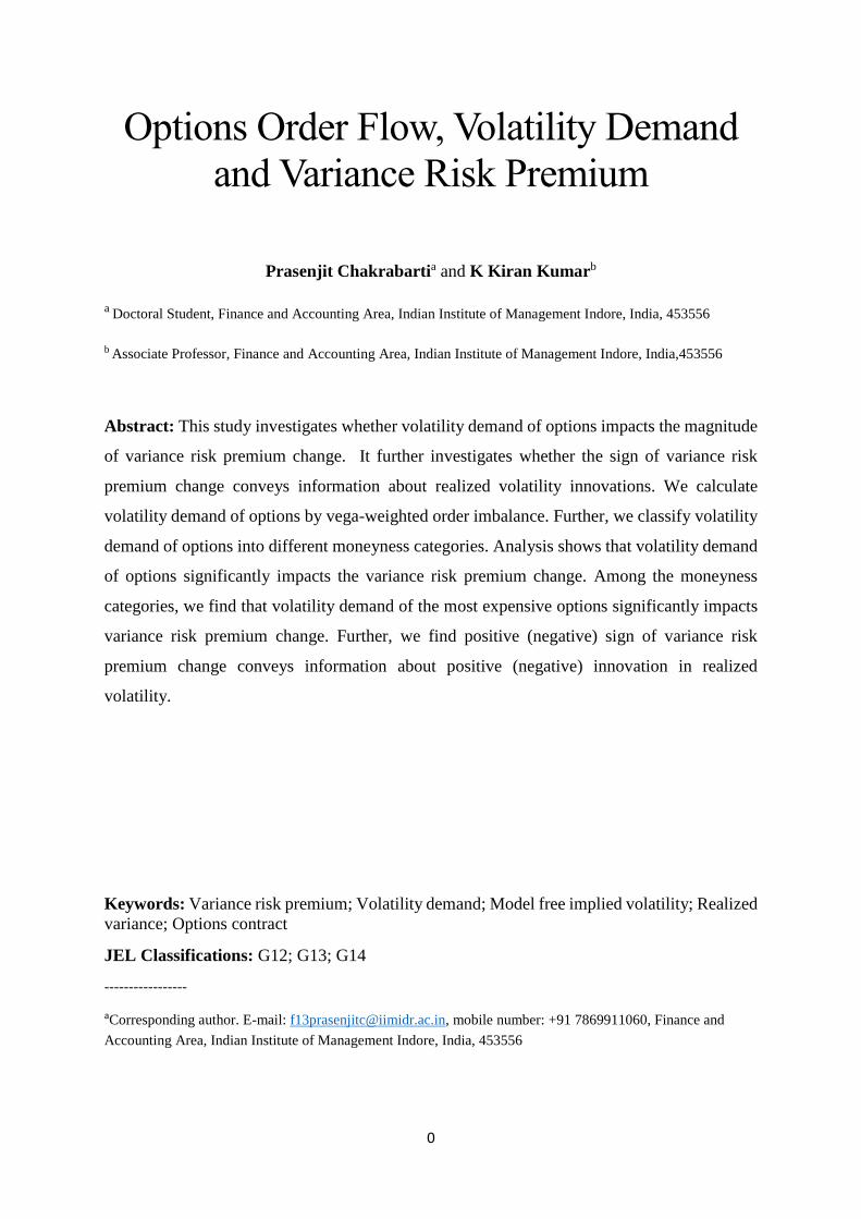
Table 2 reports the number of Nifty options traded for the period of 01 July, 2015 to 31
December, 2015.
15
Table 2: Summary of the number of Nifty options traded for the period of 1 July, 2015 to 31 December, 2015
This table summarizes the total number of call purchase, total number of put purchase across categories classified by moneyness of the options. It
also presents the net purchase of call and put options across categories. Categories are defined in Table 1.
Category Buy Call Sell Call Buy Put Sell Put Call Contracts Put Contracts Call Put
No. of
contracts
Proportion
of contracts
No. of
contracts
Proportion
of contracts
Net
purchase
of
contracts
Net
purchase
of
contracts
Category 01 (DITM_CE
and
DOTM_PE)
337550 334400 19500
23475
671950
0.000039
42975
0.000002
3150
-3975
Category 02
(ITM_CE and
OTM_PE)
46436025
46523975
1499116125
1543271775
92960000
0.005394
3042387900
0.176538
-87950
-44155650
Category 03
(ATM_CE
and
ATM_PE)
2919770975
3001981825
2544880225
2630805125
5921752800
0.343617
5175685350
0.300325
-82210850
-85924900
Category 04
(OTM_CE
and ITM_PE)
1417336475
1457551150
61255950
63846525
2874887625
0.166819
125102475
0.007259
-40214675
-2590575
Category 05
(DOTM_CE
and
DITM_PE)
18000 22725
44100
36425
40725 0.000002
80525
0.000005
-4725
7675
Total 4383899025
4506414075
4105315900
4237983325
8890313100 0.5159 8343299225
0.4841 -122515050
-132667425

16
Trading activity of the Nifty options reveals some important aspects. First, total trading activity
on call options (51.59%) is greater than on put options (48.41%). Unlike the developed
markets, where trading activity in put index options is greater than call index options
(especially S&P 500 index options), the Indian market has greater trading activity on call
options than on put options. Second, moneyness wise, trading activity on ATM call and ATM
put are largest compared to other moneyness categories. Moreover, proportion of trading
activity on ATM call options (34.36%) is substantially greater than ATM put options (30.03%).
OTM put and OTM call are the next largest traded options (OTM call contributes 16.68% and
OTM put contributes 17.65%). ITM call and ITM put come next as contributors to trading
activity. However, percentage wise their contribution is much less (ITM call 0.53% and ITM
put 0.72%). Third, interestingly, the net purchase shows that the market is a net seller of options
across all categories except DITM put and DITM call. But the proportion of DITM put and
DITM call are negligible. For that matter, trading activity proportion in Category01 and
Category05 are negligible. Therefore we ignore Category01 and Category05 for all empirical
tests.
4.3.2 Variance risk premium
We calculated variance risk premium (VRP) by Equation (1) i.e. 𝑉𝑅𝑃𝑡=𝐼𝑉𝐼𝑋𝑡2 − 𝑅𝑉𝑡,𝑡+30
2 .
We took risk neutral variance by squared India VIX (transforming into its one month variance
terms), which is calculated by the model free implied volatility (MFIV) framework, as proxy.
We calculated ex-post realized variance by the sum of five-minute squared returns over thirty
calendar days. NSE disseminates India VIX in terms of annualized volatility. We squared India
VIX and divided it by 12 to transform it into monthly variance. Below is the summary statistics
of 𝑉𝑅𝑃𝑡, ∆𝑉𝑅𝑃𝑡, |∆𝑉𝑅𝑃|𝑡, 𝑀𝐹𝐼𝑉𝑡 and 𝑅𝑉𝑡, along with Nifty returns (𝑅𝑁𝑖𝑓𝑡𝑦𝑡).
Table 3: Panel A is the descriptive statistics of monthly variance risk premium (𝑉𝑅𝑃𝑡), daily
change of variance risk premium (∆𝑉𝑅𝑃𝑡), daily magnitude change of variance risk premium
(|∆𝑉𝑅𝑃𝑡| ), realized variance (𝑅𝑉𝑡) (monthly), Model free implied variance (𝑀𝐹𝐼𝑉𝑡) (monthly),
and daily return of Nifty (𝑅𝑁𝑖𝑓𝑡𝑦𝑡) for the period 01 July, 2015 to 31 December, 2015.

17
Panel A:
𝑉𝑅𝑃𝑡 ∆𝑉𝑅𝑃𝑡 |∆𝑉𝑅𝑃𝑡| 𝑀𝐹𝐼𝑉𝑡 𝑅𝑉𝑡 𝑅𝑁𝑖𝑓𝑡𝑦𝑡 Mean
(t-statistics)
0.00084*
(1.85)
-0.00001
(-0.25)
0.00027***
(3.44)
0.00272***
(7.37)
0.00187***
(4.53)
-0.05123
(-0.55)
Median 0.00117 -0.00004 0.00015 0.00228 0.00146 -0.00995
Maximum 0.00407 0.00305 0.00305 0.00708 0.00482 2.26230
Minimum -0.00284 -0.00186 0.0000004 0.00143 0.00070 -4.49811
Std. Dev. 0.00162 0.00053 0.00045 0.00115 0.00118 0.82708
Skewness -0.73731 2.8821 4.4434 1.7141 1.3456 -1.2231
Kurtosis 3.0436 20.983 25.663 5.3637 3.5592 8.8271
Jarque-Bera (p-
value)
11.063***
(0.0039)
1798***
(0)
2987***
(0)
88.147***
(0)
38.411***
(0)
203.029***
(0)
ADF (p-value) 0.082* 0.000*** 0.000*** 0.396 0.548 0.000***
# Observations 122 121 121 122 122 122
Panel B: Correlations
𝑉𝑅𝑃𝑡 ∆𝑉𝑅𝑃𝑡 |∆𝑉𝑅𝑃𝑡| 𝑀𝐹𝐼𝑉𝑡 𝑅𝑉𝑡 𝑅𝑁𝑖𝑓𝑡𝑦𝑡 𝑉𝑅𝑃𝑡 1.0000
∆𝑉𝑅𝑃𝑡 0.1724* 1.0000
|∆𝑉𝑅𝑃|𝑡 0.2177** 0.4680*** 1.0000
𝑀𝐹𝐼𝑉𝑡 0.6815*** 0.3180*** 0.5188*** 1.0000
𝑅𝑉𝑡 -0.7054*** 0.0723 0.2051** 0.0379 1.0000
𝑅𝑁𝑖𝑓𝑡𝑦𝑡 0.0067 -0.5394*** -0.4449*** 0.1734* -0.177* 1.0000
Panel C: Autocorrelation functions
Lag 𝑉𝑅𝑃𝑡 ∆𝑉𝑅𝑃𝑡 |∆𝑉𝑅𝑃𝑡| 𝑀𝐹𝐼𝑉𝑡 𝑅𝑉𝑡 𝑅𝑁𝑖𝑓𝑡𝑦𝑡 1 0.944** 0.297** 0.477** 0.923** 0.975** 0.343 **
2 0.857** -0.156 0.235** 0.806** 0.941** 0.019
3 0.786** -0.126 0.056 0.739** 0.902** -0.055
4 0.727** -0.052 0.013 0.710** 0.859** -0.105
5 0.674** 0.093 0.124 0.688** 0.809** -0.087
Above we report in parentheses the t-statistics on the significance of mean of VRP, MFIV, RV and 𝑅𝑁𝑖𝑓𝑡𝑦𝑡 , adjusted for serial dependence by Newey-West method with 30 lags. *,**,*** denote the statistical significance at
1%, 5%, and 10% level respectively.
Panel A shows that the mean of the variance risk premium is significantly greater than zero; so
are 𝑀𝐹𝐼𝑉𝑡 and 𝑅𝑉𝑡. Thus, variance risk premium exists in Indian options and this result is
consistent with Garg and Vipul (2015). Further, mean of magnitude change of variance risk
premium (|∆𝑉𝑅𝑃𝑡|) is significantly greater than zero, which is not the case for change of
variance risk premium (∆𝑉𝑅𝑃𝑡). The standard deviation of |∆𝑉𝑅𝑃𝑡| is less than ∆𝑉𝑅𝑃𝑡. This
shows that the magnitude of variance risk premium change is less volatile than signed variance
risk premium change. 𝑉𝑅𝑃𝑡 ∆𝑉𝑅𝑃𝑡, |∆𝑉𝑅𝑃𝑡|,𝑅𝑁𝑖𝑓𝑡𝑦𝑡 series are significant after removing
trend and intercept component from them. This shows that these series are trend and intercept

18
stationary. Panel B shows the correlations among the variables. 𝑉𝑅𝑃𝑡 and 𝑅𝑉𝑡 have strong
negative correlations. On the other hand, 𝑉𝑅𝑃𝑡 and 𝑀𝐹𝐼𝑉𝑡 have strong positive correlations.
But 𝑀𝐹𝐼𝑉𝑡 and 𝑅𝑉𝑡do not show significant statistical correlations. Autocorrelation functions
of 𝑉𝑅𝑃𝑡, 𝑀𝐹𝐼𝑉𝑡 and 𝑅𝑉𝑡show that these series are strongly correlated and all the reported five
lags are significant. We observe that 𝑉𝑅𝑃𝑡maintains autocorrelations up to thirty lags though
we do not report the autocorrelation coefficients of 𝑉𝑅𝑃𝑡, 𝑀𝐹𝐼𝑉𝑡and 𝑅𝑉𝑡series here for
brevity. ∆𝑉𝑅𝑃𝑡 does not show autocorrelation more than one lag. Similarly, |∆𝑉𝑅𝑃𝑡| does not
show autocorrelation more than two lags.
Figure 1 shows the realized variance and model free implied variance (MFIV) plot for the
period 1 July, 2015 to 31 December, 2015. It is observed that MFIV is consistently higher up
to mid-July, and after the month of August i.e., from the starting of September, 2015.
Figure 1: Realized variance and MFIV plot (01Jul2015 to 31Dec2015)
One reason of MFIV being less than RV, especially during the month of August 2015, may be
because of distress in the market due to the China slowdown that affected Indian market
significantly. We plot the VRP (variance risk premium) dynamics for the period 1 July, 2015
to 31 December, 2015 in Figure 2. We observe that VRP is less than zero during mid-July to
August, 2015. This may be due to the reason stated above. Previous studies Bollerslev et al.,
0
0.001
0.002
0.003
0.004
0.005
0.006
0.007
0.008
26-May-15 15-Jul-15 03-Sep-15 23-Oct-15 12-Dec-15 31-Jan-16
Realized Variance and MF Implied Variance plot (01Jul2015 to
31Dec2015)
MF Implied variance Realized variance

19
2009, 2011; Bekaert and Hoerova, 2014; relate the variance risk premium with the market wide
risk aversion. Economic intuition is straight forward in case of positive variance risk premium.
But what is puzzling is the economic intuition of negative variance risk premium. Fan et
al.(2014) argue that the sign of negative volatility risk premium can be related to the delta-
hedged gains or losses of volatility short portfolios.
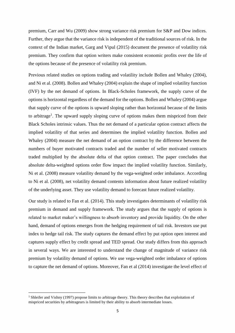
Figure 2: VRP dynamics plot (01Jul2015 to 31Dec2015)
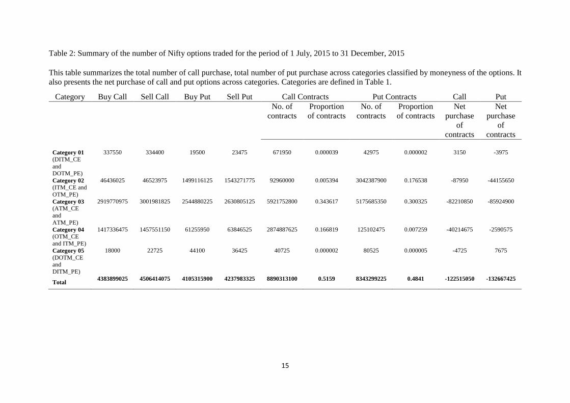
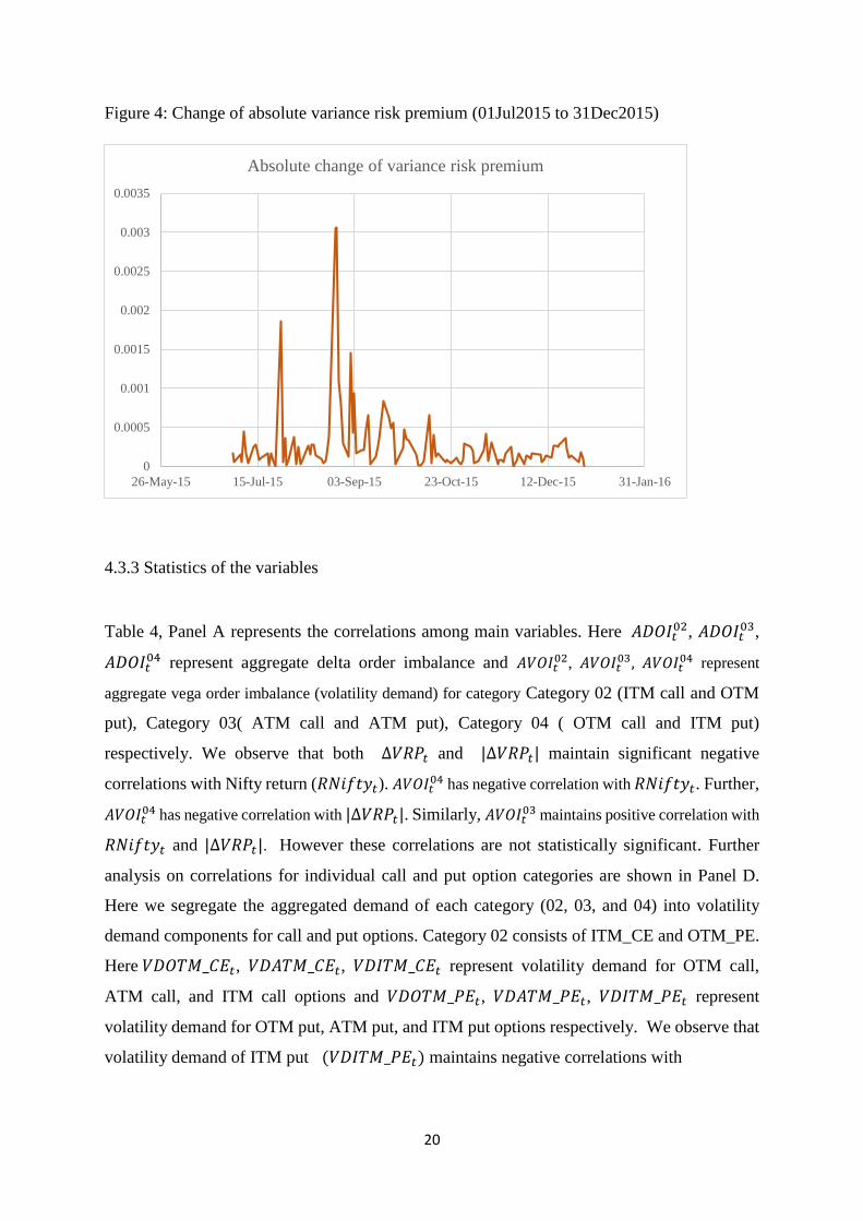
We plot the change of variance risk premium and magnitude change of variance risk premium
in Figure 3 and Figure 4.
Figure 3: Change of variance risk premium (01Jul2015 to 31Dec2015)
-0.004
-0.003
-0.002
-0.001
0
0.001
0.002
0.003
0.004
0.005
26-May-15 15-Jul-15 03-Sep-15 23-Oct-15 12-Dec-15 31-Jan-16
Variance risk premium
-0.003
-0.002
-0.001
0
0.001
0.002
0.003
0.004
26-May-15 15-Jul-15 03-Sep-15 23-Oct-15 12-Dec-15 31-Jan-16
Change of variance risk premium
20
Figure 4: Change of absolute variance risk premium (01Jul2015 to 31Dec2015)
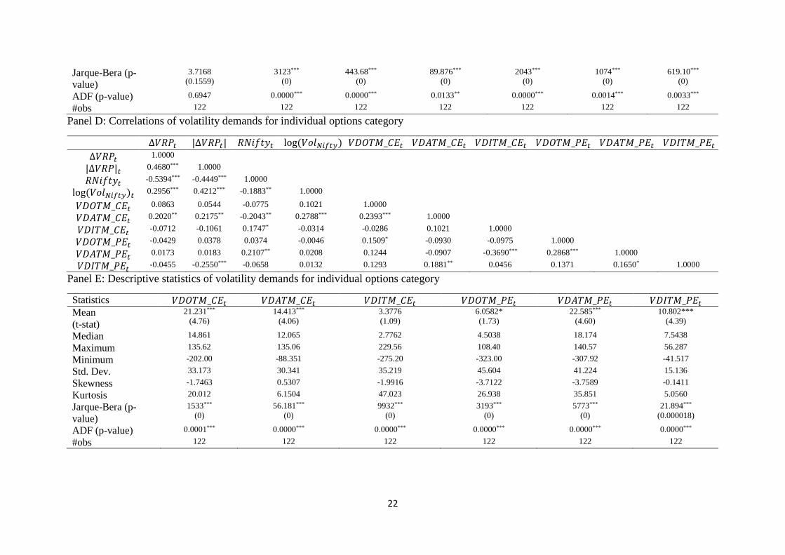
4.3.3 Statistics of the variables
Table 4, Panel A represents the correlations among main variables. Here 𝐴𝐷𝑂𝐼𝑡02, 𝐴𝐷𝑂𝐼𝑡
03,
𝐴𝐷𝑂𝐼𝑡04 represent aggregate delta order imbalance and 𝐴𝑉𝑂𝐼𝑡
02, 𝐴𝑉𝑂𝐼𝑡03, 𝐴𝑉𝑂𝐼𝑡
04 represent
aggregate vega order imbalance (volatility demand) for category Category 02 (ITM call and OTM
put), Category 03( ATM call and ATM put), Category 04 ( OTM call and ITM put)
respectively. We observe that both ∆𝑉𝑅𝑃𝑡 and |∆𝑉𝑅𝑃𝑡| maintain significant negative
correlations with Nifty return (𝑅𝑁𝑖𝑓𝑡𝑦𝑡). 𝐴𝑉𝑂𝐼𝑡04 has negative correlation with 𝑅𝑁𝑖𝑓𝑡𝑦𝑡. Further,
𝐴𝑉𝑂𝐼𝑡04 has negative correlation with |∆𝑉𝑅𝑃𝑡|. Similarly, 𝐴𝑉𝑂𝐼𝑡
03 maintains positive correlation with
𝑅𝑁𝑖𝑓𝑡𝑦𝑡 and |∆𝑉𝑅𝑃𝑡|. However these correlations are not statistically significant. Further
analysis on correlations for individual call and put option categories are shown in Panel D.
Here we segregate the aggregated demand of each category (02, 03, and 04) into volatility
demand components for call and put options. Category 02 consists of ITM_CE and OTM_PE.
Here𝑉𝐷𝑂𝑇𝑀_𝐶𝐸𝑡, 𝑉𝐷𝐴𝑇𝑀_𝐶𝐸𝑡, 𝑉𝐷𝐼𝑇𝑀_𝐶𝐸𝑡 represent volatility demand for OTM call,
ATM call, and ITM call options and 𝑉𝐷𝑂𝑇𝑀_𝑃𝐸𝑡, 𝑉𝐷𝐴𝑇𝑀_𝑃𝐸𝑡, 𝑉𝐷𝐼𝑇𝑀_𝑃𝐸𝑡 represent
volatility demand for OTM put, ATM put, and ITM put options respectively. We observe that
volatility demand of ITM put (𝑉𝐷𝐼𝑇𝑀_𝑃𝐸𝑡) maintains negative correlations with
0
0.0005
0.001
0.0015
0.002
0.0025
0.003
0.0035
26-May-15 15-Jul-15 03-Sep-15 23-Oct-15 12-Dec-15 31-Jan-16
Absolute change of variance risk premium

21
Table 4: Correlations, Autocorrelation function and summary statistics of the variables ( We report in parentheses the t-statistics on the significance of mean
adjusted for serial dependence by Newey-West method with 7 lags . *,**,*** denote the statistical significance at 1%, 5%, and 10% level respectively)
Panel A: Correlations
∆𝑉𝑅𝑃𝑡 |∆𝑉𝑅𝑃𝑡| 𝑅𝑁𝑖𝑓𝑡𝑦𝑡 log(𝑉𝑜𝑙𝑁𝑖𝑓𝑡𝑦)𝑡 𝐴𝐷𝑂𝐼𝑡02 𝐴𝐷𝑂𝐼𝑡
03 𝐴𝐷𝑂𝐼𝑡04 𝐴𝑉𝑂𝐼𝑡
02 𝐴𝑉𝑂𝐼𝑡03 𝐴𝑉𝑂𝐼𝑡
04
∆𝑉𝑅𝑃𝑡 1.0000
|∆𝑉𝑅𝑃|𝑡 0.4680*** 1.0000
𝑅𝑁𝑖𝑓𝑡𝑦𝑡 -0.5394*** -0.4449*** 1.0000
log(𝑉𝑜𝑙𝑁𝑖𝑓𝑡𝑦)𝑡 0.2956*** 0.4212*** -0.1883** 1.0000
𝐴𝐷𝑂𝐼𝑡02 -0.0800 -0.0875 0.1488 -0.0546 1.0000
𝐴𝐷𝑂𝐼𝑡03 0.0752 0.0888 -0.2336*** 0.1067 0.3790*** 1.0000
𝐴𝐷𝑂𝐼𝑡04 -0.0963 0.0125 0.1549* -0.1286 0.0827 -0.0382 1.0000
𝐴𝑉𝑂𝐼𝑡02 -0.0818 -0.0368 0.1438 -0.0247 0.3709*** -0.0201 -0.0046 1.0000
𝐴𝑉𝑂𝐼𝑡03 0.1338 0.1440 0.0491 0.1912** -0.3247*** -0.2188** -0.1059 -0.0070 1.0000
𝐴𝑉𝑂𝐼𝑡04 0.0517 -0.0569 -0.0903 0.0901 -0.0595 0.0258 -0.0751 0.1493* 0.3218*** 1.0000
Panel B: Autocorrelation function
Lag log(𝑉𝑜𝑙𝑁𝑖𝑓𝑡𝑦)𝑡 𝐴𝐷𝑂𝐼𝑡02 𝐴𝐷𝑂𝐼𝑡
03 𝐴𝐷𝑂𝐼𝑡04 𝐴𝑉𝑂𝐼𝑡
02 𝐴𝑉𝑂𝐼𝑡03 𝐴𝑉𝑂𝐼𝑡
04
1 0.512** 0.062 0.102 0.384** 0.236** 0.253** 0.416**
2 0.432** -0.018 -0.086 0.137 -0.055 0.129 0.410**
3 0.245** 0.065 0.095 0.339** -0.034 0.135 0.276**
4 0.193** -0.063 0.062 0.181** -0.096 0.047 0.181**
5 0.166** -0.061 -0.046 0.029 -0.065 0.054 0.134
Panel C: Descriptive statistics of the main variables
Statistics log(𝑉𝑜𝑙𝑁𝑖𝑓𝑡𝑦)𝑡 𝐴𝐷𝑂𝐼𝑡02 𝐴𝐷𝑂𝐼𝑡
03 𝐴𝐷𝑂𝐼𝑡04 𝐴𝑉𝑂𝐼𝑡
02 𝐴𝑉𝑂𝐼𝑡03 𝐴𝑉𝑂𝐼𝑡
04
Mean
(t-stat)
18.884***
(476.79)
0.0141**
(2.04)
-0.0045
(-1.46)
-0.0709***
(-5.01)
9.3939*
(1.85)
36.978***
(5.98)
31.924***
(5.28)
Median 18.860 0.0159 -0.0038 -0.0383 7.1742 33.181 24.131
Maximum 19.590 0.5172 0.1940 0.1312 166.33 183.35 131.06
Minimum 18.327 -0.4598 -0.0998 -0.4143 -362.80 -284.46 -202.05
Std. Dev. 0.2410 0.0780 0.0336 0.0960 54.805 49.566 38.205
Skewness 0.3973 -0.1881 1.3528 -1.6483 -3.1185 -1.7445 -1.3330
Kurtosis 3.3156 27.785 11.942 5.6100 22.056 17.112 13.709
22
Jarque-Bera (p-
value)
3.7168
(0.1559)
3123***
(0)
443.68***
(0)
89.876***
(0)
2043***
(0)
1074***
(0)
619.10***
(0)
ADF (p-value) 0.6947 0.0000*** 0.0000*** 0.0133** 0.0000*** 0.0014*** 0.0033***
#obs 122 122 122 122 122 122 122
Panel D: Correlations of volatility demands for individual options category
∆𝑉𝑅𝑃𝑡 |∆𝑉𝑅𝑃𝑡| 𝑅𝑁𝑖𝑓𝑡𝑦𝑡 log(𝑉𝑜𝑙𝑁𝑖𝑓𝑡𝑦)𝑡 𝑉𝐷𝑂𝑇𝑀_𝐶𝐸𝑡 𝑉𝐷𝐴𝑇𝑀_𝐶𝐸𝑡 𝑉𝐷𝐼𝑇𝑀_𝐶𝐸𝑡 𝑉𝐷𝑂𝑇𝑀_𝑃𝐸𝑡 𝑉𝐷𝐴𝑇𝑀_𝑃𝐸𝑡 𝑉𝐷𝐼𝑇𝑀_𝑃𝐸𝑡
∆𝑉𝑅𝑃𝑡 1.0000
|∆𝑉𝑅𝑃|𝑡 0.4680*** 1.0000
𝑅𝑁𝑖𝑓𝑡𝑦𝑡 -0.5394*** -0.4449*** 1.0000
log(𝑉𝑜𝑙𝑁𝑖𝑓𝑡𝑦)𝑡 0.2956*** 0.4212*** -0.1883** 1.0000
𝑉𝐷𝑂𝑇𝑀_𝐶𝐸𝑡 0.0863 0.0544 -0.0775 0.1021 1.0000
𝑉𝐷𝐴𝑇𝑀_𝐶𝐸𝑡 0.2020** 0.2175** -0.2043** 0.2788*** 0.2393*** 1.0000
𝑉𝐷𝐼𝑇𝑀_𝐶𝐸𝑡 -0.0712 -0.1061 0.1747* -0.0314 -0.0286 0.1021 1.0000
𝑉𝐷𝑂𝑇𝑀_𝑃𝐸𝑡 -0.0429 0.0378 0.0374 -0.0046 0.1509* -0.0930 -0.0975 1.0000
𝑉𝐷𝐴𝑇𝑀_𝑃𝐸𝑡 0.0173 0.0183 0.2107** 0.0208 0.1244 -0.0907 -0.3690*** 0.2868*** 1.0000
𝑉𝐷𝐼𝑇𝑀_𝑃𝐸𝑡 -0.0455 -0.2550*** -0.0658 0.0132 0.1293 0.1881** 0.0456 0.1371 0.1650* 1.0000
Panel E: Descriptive statistics of volatility demands for individual options category
Statistics 𝑉𝐷𝑂𝑇𝑀_𝐶𝐸𝑡 𝑉𝐷𝐴𝑇𝑀_𝐶𝐸𝑡 𝑉𝐷𝐼𝑇𝑀_𝐶𝐸𝑡 𝑉𝐷𝑂𝑇𝑀_𝑃𝐸𝑡 𝑉𝐷𝐴𝑇𝑀_𝑃𝐸𝑡 𝑉𝐷𝐼𝑇𝑀_𝑃𝐸𝑡 Mean
(t-stat)
21.231***
(4.76)
14.413***
(4.06)
3.3776
(1.09)
6.0582*
(1.73)
22.585***
(4.60)
10.802***
(4.39)
Median 14.861 12.065 2.7762 4.5038 18.174 7.5438
Maximum 135.62 135.06 229.56 108.40 140.57 56.287
Minimum -202.00 -88.351 -275.20 -323.00 -307.92 -41.517
Std. Dev. 33.173 30.341 35.219 45.604 41.224 15.136
Skewness -1.7463 0.5307 -1.9916 -3.7122 -3.7589 -0.1411
Kurtosis 20.012 6.1504 47.023 26.938 35.851 5.0560
Jarque-Bera (p-
value)
1533***
(0)
56.181***
(0)
9932***
(0)
3193***
(0)
5773***
(0)
21.894***
(0.000018)
ADF (p-value) 0.0001*** 0.0000*** 0.0000*** 0.0000*** 0.0000*** 0.0000***
#obs 122 122 122 122 122 122

23
∆𝑉𝑅𝑃𝑡, |∆𝑉𝑅𝑃𝑡|, and 𝑅𝑁𝑖𝑓𝑡𝑦𝑡. Further, the negative correlation is statistically significant for
|∆𝑉𝑅𝑃𝑡|. On the other hand, 𝑉𝐷𝑂𝑇𝑀_𝐶𝐸𝑡 shows positive correlation with |∆𝑉𝑅𝑃𝑡|, and it is
not statistically significant and lower in terms of absolute value. So, we assume that increase
in volatility demand of 𝑉𝐷𝐼𝑇𝑀_𝑃𝐸𝑡 decreases absolute change of variance risk premium; in
turn Category 04 options negatively impacts|∆𝑉𝑅𝑃𝑡|. Both 𝑉𝐷𝐴𝑇𝑀_𝐶𝐸𝑡 and 𝑉𝐷𝐴𝑇𝑀_𝑃𝐸𝑡
maintain positive correlation with |∆𝑉𝑅𝑃𝑡|, therefore we assume ATM options ( Category 03)
impacts |∆𝑉𝑅𝑃𝑡| positively. That is increase in volatility demand of ATM options
increases|∆𝑉𝑅𝑃𝑡|. Category 02 options (𝑉𝐷𝑂𝑇𝑀_𝑃𝐸𝑡,𝑉𝐷𝐼𝑇𝑀_𝐶𝐸𝑡) show opposite
correlations with |∆𝑉𝑅𝑃𝑡| and none of them is statistically significant.
Panel B shows autocorrelation function of the main variables. We observe
log(𝑉𝑜𝑙𝑁𝑖𝑓𝑡𝑦)𝑡 has significant autocorrelations up to seven lags. We do not report the
coefficients up to ten lags due to brevity. Therefore, we choose Newey-West t-statistics with
seven lags.
Panel C and Panel E shows summary statistics of the variables. Mean of all the aggregated
volatility demand components𝐴𝑉𝑂𝐼𝑡02,𝐴𝑉𝑂𝐼𝑡
03, 𝐴𝑉𝑂𝐼𝑡04 are significantly positive. In case of
individual options, mean of all the put option’s volatility demand are significantly positive,
whereas mean of volatility demand at OTM and ATM call options are significantly positive.
All these variables (aggregated and individual volatility demand) are stationary.5 Next we
discuss the pattern of the implied volatility skew for the period of study.
4.3.4 Implied volatility skew
We compute the Black Scholes implied volatility skew of the options for the period 1 July,
2015 to 31 December, 2015. We observe that volatility skew of Nifty options form forward
skew.
Figure 5: Implied volatility skew of Nifty options
5 Note that trading volume is not stationary. We do not detrend volume following Lo and Wang (2000). They
fail to detrend the volume without adequately removing serial correlation. Therefore, the paper advises to take
shorter interval when analyzing trading volume (typically 5 years). Our study period interval is only 6 months.

24
The volatility skew pattern shows that OTM call options and ITM put options are expensive.
Further, we observe that ITM put options are even more expensive than OTM call options.
5. Empirical results
In the empirical test section, we start with Equation 9, where we regress change of variance
risk premium with the set of independent variables and control variables as mentioned in the
equation specification.
5.1 Empirical results (change of variance risk premium)
Table 5 reports the result of Equation 9. Results show that aggregate delta order imbalances (
𝐴𝐷𝑂𝐼𝑡02,𝐴𝐷𝑂𝐼𝑡
03, 𝐴𝐷𝑂𝐼𝑡04) do not have any statistical significance on the changes of variance
risk premium for Models (2) and (3). Further, aggregate volatility demands (𝐴𝑉𝑂𝐼𝑡02,𝐴𝑉𝑂𝐼𝑡
03,
𝐴𝑉𝑂𝐼𝑡04) do not show any statistical significance in Model (4) except in Model (2), where
𝐴𝑉𝑂𝐼𝑡02 impacts change of variance risk premium negatively. 𝐴𝑑𝑗𝑅2 of the models show that
Model (1) best explains the relationship, followed by Model (4). For all the models, coefficients
0
20
40
60
80
100
120
BS
Im
pli
ed V
ola
tili
ty(%
)
Moneyness
Implied Volatility Skew -Nifty Index options (01Jul2015 to
31Dec2015)
Call Skew Put Skew
ATM Call
ATM Put
ITM Put
OTM Call

25
of aggregate delta order imbalance and aggregate vega order imbalance maintain consistency
in their signs. We observe that coefficient of 𝐴𝐷𝑂𝐼𝑡04 have negative signs
Table 5: Results of Equation (9)
∆𝑉𝑅𝑃𝑡 = 𝛼0 + 𝜇𝐶𝑜𝑛𝑡𝑟𝑜𝑙𝑡 + ∑ 𝛾𝑡𝑐𝑎𝑡𝐴𝑉𝑂𝐼𝑡
𝑐𝑎𝑡 + 𝛿𝑡∆𝑉𝑅𝑃𝑡−1+휀𝑐𝑎𝑡 .Models (1), (2), (3), and (4)
are the GMM estimates of the variables shown in the table. t-statistics are computed according
to Newey and West (1987) with 7 lags. *,**,*** denote the statistical significance at 1%, 5%, and
10% levels respectively.
Variable (1) (2) (3) (4)
𝐼𝑛𝑡𝑒𝑟𝑐𝑒𝑝𝑡 -0.00719*
(-1.96)
-0.0063*
(-1.84)
-0.00718*
(-1.90)
-0.00644*
(-1.91)
𝑅𝑁𝑖𝑓𝑡𝑦𝑡 -0.00031***
(-2.91)
-0.00033***
(-2.66)
-0.00032***
(-2.88)
-0.00031**
(-2.61)
log(𝑉𝑜𝑙𝑁𝑖𝑓𝑡𝑦)𝑡 0.00037*
(1.95)
0.00032*
(1.82)
0.000377*
(1.89)
0.00033*
(1.90)
𝐴𝐷𝑂𝐼𝑡02 0.00093
(1.49)
0.00043
(0.85)
𝐴𝐷𝑂𝐼𝑡03 -0.00135
(-1.66)
-0.00133
(-1.38)
𝐴𝐷𝑂𝐼𝑡04 -0.00018
(-0.48)
-0.00019
(-0.53)
𝐴𝑉𝑂𝐼𝑡02(× 10−6) -0.861*
(-1.70)
-0.345
(-0.51)
𝐴𝑉𝑂𝐼𝑡03 (× 10−6) 1.347
(0.96)
1.166
(0.99)
𝐴𝑉𝑂𝐼𝑡04(× 10−6) -0.489
(-0.30)
-0.580
(-0.36)
∆𝑉𝑅𝑃𝑡−1 0.2026**
(2.30)
0.2228**
(2.62)
0.2179**
(2.59)
0.1941**
(2.16)
𝐴𝑑𝑗𝑅2 0.3549 0.3465
0.3451 0.3506
#Obs 120 120 120 120
for all the models. Similarly, coefficients of 𝐴𝐷𝑂𝐼𝑡03 have positive signs and coefficients of
𝐴𝐷𝑂𝐼𝑡02 have negative signs. Coefficients of ∆𝑉𝑅𝑃𝑡−1 have positive signs for all the models.
Continuing with Hypothesis 1, we test whether Equation (10) with magnitude of absolute
change of variance risk premium as dependent variable can provide us better insights about the
relationship. The results of Equation (1) can be found in Table 6.
5.2 Empirical results (magnitude of variance risk premium change)

26
Table 6 shows the result of Equation (10). The magnitude regression improves 𝐴𝑑𝑗𝑅2 for all
the models. In the magnitude regression, Model (4) best explains the relationship among all
other models.
Table 6: Results of Equation (10)
|∆𝑉𝑅𝑃𝑡| = 𝛼0 + 𝜇𝐶𝑜𝑛𝑡𝑟𝑜𝑙𝑡 + ∑ 𝛼𝑡𝑐𝑎𝑡𝐴𝑉𝑂𝐼𝑡
𝑐𝑎𝑡 + 𝛽𝑡|∆𝑉𝑅𝑃𝑡−1| + 휀𝑐𝑎𝑡 .Models (1), (2), (3),
and (4) are the GMM estimates of the variables shown in the table. t-statistics are computed
according to Newey and West (1987) with 7 lags. *,**,*** denote the statistical significance at
1%, 5%, and 10% levels respectively.
Variable (1) (2) (3) (4)
𝐼𝑛𝑡𝑒𝑟𝑐𝑒𝑝𝑡 -0.00766**
(-2.11)
-0.00751**
(-2.11)
-0.00787**
(-2.11)
-0.00729**
(-2.09)
𝑅𝑁𝑖𝑓𝑡𝑦𝑡 -0.00021**
(-2.27)
-0.00024**
(-2.32)
-0.00022**
(-2.15)
-0.00022**
(-2.41)
log(𝑉𝑜𝑙𝑁𝑖𝑓𝑡𝑦)𝑡 0.00041**
(2.15)
0.00040**
(2.15)
0.00042**
(2.15)
0.00039**
(2.13)
𝐴𝐷𝑂𝐼𝑡02 0.00027
(0.78)
0.00016
(0.46)
𝐴𝐷𝑂𝐼𝑡03 -0.00079
(-0.81)
-0.0010
(-0.96)
𝐴𝐷𝑂𝐼𝑡04 0.00021
(0.68)
0.00018
(0.57)
𝐴𝑉𝑂𝐼𝑡02(× 10−6) 0.142
(0.32)
0.261
(0.50)
𝐴𝑉𝑂𝐼𝑡03 (× 10−6) 1.184*
(1.76)
1.131*
(1.85)
𝐴𝑉𝑂𝐼𝑡04(× 10−6) -1.93
(-1.53)
-1.99
(-1.54)
|∆𝑉𝑅𝑃𝑡−1| 0.3710***
(2.83)
0.3599***
(2.95)
0.3749***
(2.83)
0.3598***
𝐴𝑑𝑗𝑅2 0.4241 0.4290 0.4154 0.4391
#Obs 120 120 120 120
We observe that 𝐼𝑛𝑡𝑒𝑟𝑐𝑒𝑝𝑡, 𝑅𝑁𝑖𝑓𝑡𝑦𝑡 , and log(𝑉𝑜𝑙𝑁𝑖𝑓𝑡𝑦)𝑡 do not change their signs with
absolute value change of variance risk premium. In the Equation (10), 𝐴𝐷𝑂𝐼𝑡04 and 𝐴𝑉𝑂𝐼𝑡
02
reverse their signs. Everything else maintain consistency in terms of their signs. For Model (2)
and Model (4) volatility demand of ATM options remain statistically significant. Further,
volatility demand of ATM options positively impacts the magnitude change of variance risk
premium. The reason could be that ATM options are most sensitive to volatility change.
Therefore, market participants with volatility information would prefer to trade in ATM
options. Moreover, in Table 1, we see that ATM options are the most traded options in the list

27
of all the categories. For all the categories of options, it is seen that delta order imbalances do
not have any impact on change of variance risk premium, which is as per our expectation.
Coefficients of nifty returns (𝑅𝑁𝑖𝑓𝑡𝑦𝑡) by both Equations (9) and (10), for all the models are
consistently negative. That is as per our expectation and consistent with the previous studies of
Giot 2005; Whaley 2009; Badshah 2013; Chakrabarti 2015, that state negative returns increases
the implied volatility and high volatility is a representative of high risk (Hibbert et al. 2008;
Badshah 2013). Increase in implied volatility in turn increases variance risk premium; thus,
Nifty returns have negative impact on change as well as on magnitude change of variance risk
premium.
Coefficients of logarithm volume are positive for Equations (9) and (10), for all the models as
per expectation. This is because higher trading volume implies lower volatility (Bessembinder
and Seguin, 1992) and lower volatility in turn lowers the magnitude of variance risk premium.
Table 6 shows that volatility demand of ATM options have significant positive impact on the
magnitude of variance risk premium change. We further regress magnitude of variance risk
premium change with the volatility demand of individual call and put options.
5.3 Empirical results (magnitude of variance risk premium change with volatility
demand of call and put options)
We report the results of the regression in Table 7. Results show that 𝐴𝑑𝑗𝑅2 of the model
increases with volatility demand components of call and put options. Further, we see that
volatility demand at ATM and ITM put options are statistically significant. Volatility demand
of call options is insignificant. Volatility demand of ATM put options has positive impact on
the magnitude of variance risk premium change, whereas, ITM put options have negative
impact on magnitude of variance risk premium change. The sign of the impact is evident from
the correlation analysis in Table 4, where we have seen that volatility demand at ITM put
options maintain negative correlation with magnitude of variance risk premium change, and
ATM put options have positive correlation with magnitude of variance risk premium change.
Another support for the evidence is the volatility skew pattern for the period of study. We see
that ATM and ITM put options are expensive, relative to other put options. So volatility trading
activity at ATM and ITM put options may have impact on the magnitude of variance risk
premium.

28
Table 7: Results of equation
|∆𝑉𝑅𝑃𝑡| = 𝛼0 + 𝜇𝐶𝑜𝑛𝑡𝑟𝑜𝑙𝑡 + ∑ 𝛼𝑡𝐶𝑎𝑙𝑙,𝑝𝑢𝑡𝑉𝐷𝑖 + 𝛽𝑡|∆𝑉𝑅𝑃𝑡−1| + 휀𝑐𝑎𝑙𝑙,𝑝𝑢𝑡 .Model (1) is the
GMM estimates of the variables shown in the Table. t-statistics are computed according to
Newey and West (1987) with 7 lags. *,**,*** denote the statistical significance at 1%, 5%, and
10% levels respectively.
Variable (1)
𝐼𝑛𝑡𝑒𝑟𝑐𝑒𝑝𝑡 -0.00762 **
(-2.22)
𝑅𝑁𝑖𝑓𝑡𝑦𝑡 -0.00024 **
(-2.41)
log(𝑉𝑜𝑙𝑁𝑖𝑓𝑡𝑦)𝑡 0.00041 **
(2.15)
𝑉𝐷𝑂𝑇𝑀_𝐶𝐸𝑡(× 10−6) -0.869
(-0.85)
𝑉𝐷𝐴𝑇𝑀_𝐶𝐸𝑡(× 10−6) 0.834
(0.94)
𝑉𝐷𝐼𝑇𝑀_𝐶𝐸𝑡(× 10−6) 0.791
(0.75)
𝑉𝐷𝑂𝑇𝑀_𝑃𝐸𝑡(× 10−6) 0.274
(0.79)
𝑉𝐷𝐴𝑇𝑀_𝑃𝐸𝑡 (× 10−6) 1.81*
(1.81)
𝑉𝐷𝐼𝑇𝑀_𝑃𝐸𝑡(× 10−6) -6.74***
(-2.92)
|∆𝑉𝑅𝑃𝑡−1| 0.3034***
(2.66)
𝐴𝑑𝑗𝑅2 0.4489
#Obs 120
From the analysis of Table 5 and Table 6 it is evident that Equation (10) better describes the
relationship between magnitude of variance risk premium and volatility demand of options. It
is apparent that the sign of the variance risk premium change introduces additional noise, which
makes the explanation difficult. With the magnitude of variance risk premium change as
dependent variable, the statistical clarity of the data increases.
5.4 Empirical results (robustness checks)

29
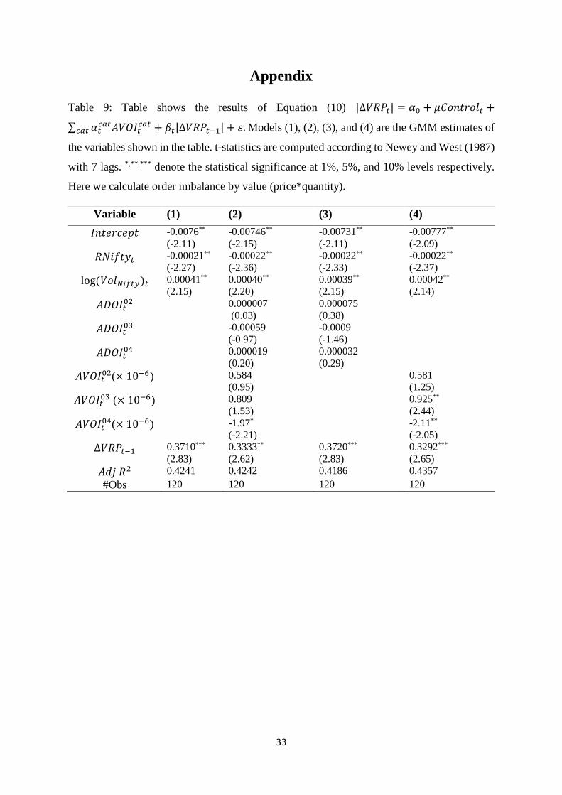
We conduct robustness tests of our models. We have done first robustness test by taking order
imbalance in terms of value (quantity*price) in magnitude regression. Table 9 reports the
results. We see that estimates are consistent, with no meaningful change in the result other than
magnitude of the estimated coefficients.
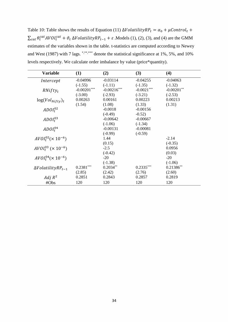
Volatility is non-linear monotone transformation of variance. Thus, we also estimate the
coefficients with change (absolute change) of volatility risk premium. Results are reported in
Table 10, Table 11 and Table 12. We observe that results are mostly consistent when we
estimate coefficients taking change of volatility risk premium. No meaningful change is
observed. When we estimate coefficients with the magnitude of the volatility risk premium
change, results are consistent with the results of magnitude of variance risk premium change
throughout, other than magnitude of the estimated coefficients. Table 9, Table 10, Table 11,
and Table 12 are included in Appendix.
These empirical tests confirm Hypothesis 1 i.e., change in net volatility demand influences the
change in variance risk premium.
5.5 Empirical results (Sign test)
We test Hypothesis 2 by Equation (13). The results can be found in Table 8. According to our
hypothesis, sign of variance risk premium change should indicate expectation about the change
of realized volatility. We expect a positive coefficient of𝑠𝑖𝑔𝑛(∆𝑉𝑅𝑃𝑡), because if the
hypothesis holds true , a positive (negative) sign should indicate increase (decrease) in realized
volatility. Results of Equation (8) shows that coefficient of 𝑠𝑖𝑔𝑛(∆𝑉𝑅𝑃𝑡) is positive and
statistically significant at 10% level. This result confirms Hypothesis 2, although the 𝐴𝑑𝑗𝑅2 is
less.
Table 8: Results of Equation 13
∆𝑅𝑉𝑡 = 𝛼0 + 𝛼1𝑠𝑖𝑔𝑛(∆𝑉𝑅𝑃𝑡) + 휀. Model (1) is the GMM estimates of the variables shown
in Table. t-statistics are computed according to Newey and West (1987) with 30 lags. *,**,***
denote the statistical significance at 1%, 5%, and 10% levels respectively.
Variable (1)
𝐼𝑛𝑡𝑒𝑟𝑐𝑒𝑝𝑡 0.000052 *
(1.74)

30
∆𝑅𝑉𝑡 0.000029 *
(1.82)
𝐴𝑑𝑗𝑅2 0.0161
#Obs 120
Fan et al. (2014) discuss that the sign of volatility risk premium contents the information of
delta-hedged gains or losses of option portfolios. Further analysis in this regard can be taken
up in the course of future studies.
6. Conclusion
In this paper, we investigate whether volatility demand of options impacts the magnitude of
variance risk premium change. We further investigate whether the sign of variance risk
premium change conveys information about realized volatility innovations. We calculate
aggregated volatility demand by vega-weighted order imbalance. Further, we classify
aggregated volatility demand of options into different moneyness categories.
Analysis shows that aggregated volatility demand of options significantly impacts the
magnitude of variance risk premium change. We explore the nature of impact for different
moneyness categories. Results show that aggregated volatility demand at ATM options
positively impacts variance risk premium. Further we analyse the impact of volatility demand
of call and put options on magnitude of variance risk premium change. We find, volatility
demand of ATM and ITM put options significantly impact the variance risk premium change.
Volatility skew pattern (for the period of study) supports this finding, as ATM and ITM put
options remain expensive for the period of study. We conduct several robustness tests of our
results. These test results show that findings of the study are also consistent with volatility risk
premium.
We find that the sign of variance risk premium change conveys information about realized
volatility innovations. Positive (negative) sign of variance risk premium change indicates
positive (negative) realized volatility innovation.
Thus, the study concludes that volatility demand information in options order flow impacts the
volatility/variance risk premium, while nature and degree of the impact depend on the market
structure.

31
References
Ait-Sahalia, Y., Karaman, M., and Mancini, L. “The term structure of variance swaps, risk premia and
the expectation hypothesis.”, (2013), Working paper, Princeton University.
Badshah, I.U. “Quantile regression analysis of the asymmetric return‐volatility relation.” Journal of
Futures Markets, 33, (2013), pp. 235-265.
Bakshi, G., and Kapadia, N.”Delta-hedged gains and the negative market volatility risk
premium.” Review of Financial Studies, 16, (2003), pp. 527-566.
Bekaert, G., and Hoerova, M. “The VIX, the variance premium and stock market volatility. “Journal of
Econometrics, 183, (2014), pp. 181-192.
Bessembinder, H., and Seguin, P. J. “Futures‐trading activity and stock price volatility.” Journal of
Finance, 47, (1992), pp. 2015-2034.
Black, F. "The pricing of commodity contracts." Journal of Financial Economics, 3, (1976), pp. 167–
179.
Black, F. “Fact and Fantasy in Use of Options.” Financial Analysts Journal, 31, (1975), pp. 61-72.
Bollen, N. P., and Whaley, R. E. "Does net buying pressure affect the shape of implied volatility
functions?" Journal of Finance, 59, (2004), pp. 711-753.
Bollerslev, T., Gibson, M., and Zhou, H. “Dynamic estimation of volatility risk premia and investor
risk aversion from option-implied and realized volatilities.” Journal of econometrics, 160, (2011), pp.
235-245.
Bollerslev, T., Tauchen, G., and Zhou, H. “Expected stock returns and variance risk premia." Review
of Financial Studies, 22, (2009), pp. 4463-4492.
Britten‐Jones, M., and Neuberger, A. “Option prices, implied price processes, and stochastic volatility.”
Journal of Finance, 55, (2000), pp. 839-866.
Carr, P., and Wu, L. "Variance risk premiums." Review of Financial Studies, 22, (2009), pp. 1311-
1341.
Chakrabarti, P. "Examining Contemporaneous Relationship between Return of Nifty Index and India
VIX." International Journal of Financial Management, 5, (2015), pp. 50-54.
Chakravarty, S., Gulen, H., and Mayhew, S. “Informed trading in stock and option markets.” Journal
of Finance, 59, (2004), pp. 1235-1257.
Chen, Y., Shu, J., and Zhang, J. E. "Investor sentiment, variance risk premium and delta-hedged
gains." Applied Economics, (2016), pp. 1-13.
Coval, J. D., and Shumway, T. "Expected option returns." Journal of Finance, 56, (2001), pp. 983-
1009.
Demeterfi, K., Derman, E., Kamal, M., and Zou, J. “A guide to volatility and variance swaps.” Journal
of Derivatives, 6, (1999), pp. 9-32.
Drechsler, I., and Yaron, A. "What's vol got to do with it." Review of Financial Studies, 24, (2011),
pp. 1-45.

32
Fan, J., Imerman, M. B., and Dai, W. “What does the volatility risk premium say about liquidity
provision and demand for hedging tail risk?”, (2013), Available at SSRN 2234438.
Garg, S., and Vipul. "Volatility Risk Premium in Indian Options Prices." Journal of Futures Markets,
35, (2015), pp. 795-812.
Garleanu, N., Pedersen, L. H., and Poteshman, A. M. “Demand-based option pricing.” Review of
Financial Studies, 22, (2009), pp. 4259-4299.
Giot, P. “Relationships between implied volatility indexes and stock index returns.” Journal of Portfolio
Management, 31, (2005), pp. 92-100.
Grossman, and Sanford, J. "The existence of futures markets, noisy rational expectations and
information externalities." Review of Economic Studies, 44, (1977), pp. 431–449.
Hibbert, A.M., R.T. Daigler, and B. Dupoyet. “A behavioral explanation for the negative asymmetric
return volatility relation.” Journal of Banking & Finance, 32, (2008), pp. 2254-2266.
Holowczak, R., Hu, J., and Wu, L. "Aggregating information in option transactions." Journal of
Derivatives, 21, (2014), pp. 9-23.
Lo, A. W., and Wang, J. “Trading volume: definitions, data analysis, and implications of portfolio
theory. “Review of Financial Studies, 13, (2000), pp. 257-300.
Newey, W. K., and K. D. West. “A Simple, Positive Semi-Definite, Heteroskedasticity and
Autocorrelation Consistent Covariance Matrix." Econometrica , 55, (1987), pp. 703–8.
Ni, S. X., Pan, J., and Poteshman, A. M. "Volatility information trading in the option market." Journal
of Finance, 63, (2008), pp. 1059-1091.
Shleifer, A. and R.W. Vishny. “The limits of arbitrage.” Journal of Finance, 52, (1997), pp. 35-55
Wang, Z., and Daigler, R. T. "The performance of VIX option pricing models: empirical evidence
beyond simulation." Journal of Futures Markets, 31, (2011), pp. 251-281.
Whaley, R.E. “Understanding the VIX.” Journal of Portfolio Management, 35, (2009),pp. 98-105.
33
Appendix
Table 9: Table shows the results of Equation (10) |∆𝑉𝑅𝑃𝑡| = 𝛼0 + 𝜇𝐶𝑜𝑛𝑡𝑟𝑜𝑙𝑡 +
∑ 𝛼𝑡𝑐𝑎𝑡𝐴𝑉𝑂𝐼𝑡
𝑐𝑎𝑡 + 𝛽𝑡|∆𝑉𝑅𝑃𝑡−1| + 휀𝑐𝑎𝑡 .Models (1), (2), (3), and (4) are the GMM estimates of
the variables shown in the table. t-statistics are computed according to Newey and West (1987)
with 7 lags. *,**,*** denote the statistical significance at 1%, 5%, and 10% levels respectively.
Here we calculate order imbalance by value (price*quantity).
Variable (1) (2) (3) (4)
𝐼𝑛𝑡𝑒𝑟𝑐𝑒𝑝𝑡 -0.0076**
(-2.11)
-0.00746**
(-2.15)
-0.00731**
(-2.11)
-0.00777**
(-2.09)
𝑅𝑁𝑖𝑓𝑡𝑦𝑡 -0.00021**
(-2.27)
-0.00022**
(-2.36)
-0.00022**
(-2.33)
-0.00022**
(-2.37)
log(𝑉𝑜𝑙𝑁𝑖𝑓𝑡𝑦)𝑡 0.00041**
(2.15)
0.00040**
(2.20)
0.00039**
(2.15)
0.00042**
(2.14)
𝐴𝐷𝑂𝐼𝑡02 0.000007
(0.03)
0.000075
(0.38)
𝐴𝐷𝑂𝐼𝑡03 -0.00059
(-0.97)
-0.0009
(-1.46)
𝐴𝐷𝑂𝐼𝑡04 0.000019
(0.20)
0.000032
(0.29)
𝐴𝑉𝑂𝐼𝑡02(× 10−6) 0.584
(0.95)
0.581
(1.25)
𝐴𝑉𝑂𝐼𝑡03 (× 10−6) 0.809
(1.53)
0.925**
(2.44)
𝐴𝑉𝑂𝐼𝑡04(× 10−6) -1.97*
(-2.21)
-2.11**
(-2.05)
∆𝑉𝑅𝑃𝑡−1 0.3710***
(2.83)
0.3333**
(2.62)
0.3720***
(2.83)
0.3292***
(2.65)
𝐴𝑑𝑗𝑅2 0.4241 0.4242 0.4186 0.4357
#Obs 120 120 120 120
34
Table 10: Table shows the results of Equation (11) ∆𝑉𝑜𝑙𝑎𝑡𝑖𝑙𝑖𝑡𝑦𝑅𝑃𝑡 = 𝛼0 + 𝜇𝐶𝑜𝑛𝑡𝑟𝑜𝑙𝑡 +
∑ 𝜃𝑡𝑐𝑎𝑡𝐴𝑉𝑂𝐼𝑡
𝑐𝑎𝑡 + 𝜗𝑡∆𝑉𝑜𝑙𝑎𝑡𝑖𝑙𝑖𝑡𝑦𝑅𝑃𝑡−1 + 휀.𝑐𝑎𝑡 Models (1), (2), (3), and (4) are the GMM
estimates of the variables shown in the table. t-statistics are computed according to Newey
and West (1987) with 7 lags. *,**,*** denote the statistical significance at 1%, 5%, and 10%
levels respectively. We calculate order imbalance by value (price*quantity).
Variable (1) (2) (3) (4)
𝐼𝑛𝑡𝑒𝑟𝑐𝑒𝑝𝑡 -0.04996
(-1.55)
-0.03114
(-1.11)
-0.04255
(-1.35)
-0.04063
(-1.32)
𝑅𝑁𝑖𝑓𝑡𝑦𝑡 -0.00201***
(-3.00)
-0.00216***
(-2.93)
-0.0021***
(-3.21)
-0.00201**
(-2.53)
log(𝑉𝑜𝑙𝑁𝑖𝑓𝑡𝑦)𝑡 0.00263
(1.54)
0.00161
(1.08)
0.00223
(1.33)
0.00213
(1.31)
𝐴𝐷𝑂𝐼𝑡02 -0.0018
(-0.49)
-0.00156
-0.52)
𝐴𝐷𝑂𝐼𝑡03 -0.00642
(-1.06)
-0.00667
(-1.34)
𝐴𝐷𝑂𝐼𝑡04 -0.00131
(-0.99)
-0.00081
(-0.59)
𝐴𝑉𝑂𝐼𝑡02(× 10−6) 1.44
(0.15)
-2.14
(-0.35)
𝐴𝑉𝑂𝐼𝑡03 (× 10−6) -2.5
(-0.42)
0.0956
(0.03)
𝐴𝑉𝑂𝐼𝑡04(× 10−6) -20
(-1.38)
-20
(-1.06)
∆𝑉𝑜𝑙𝑎𝑡𝑖𝑙𝑖𝑡𝑦𝑅𝑃𝑡−1 0.2381***
(2.85)
0.2034**
(2.42)
0.2335***
(2.76)
0.21386**
(2.60)
𝐴𝑑𝑗𝑅2 0.2851 0.2843 0.2857 0.2819
#Obs 120 120 120 120

35
Table 11: Table shows the results of Equation (12) |∆𝑉𝑜𝑙𝑎𝑡𝑖𝑙𝑖𝑡𝑦𝑅𝑃𝑡| = 𝛼0 + 𝜇𝐶𝑜𝑛𝑡𝑟𝑜𝑙𝑡 +
∑ 𝜇𝑡𝑐𝑎𝑡𝐴𝑉𝑂𝐼𝑡
𝑐𝑎𝑡 + 𝜋𝑡 |∆𝑉𝑜𝑙𝑎𝑡𝑖𝑙𝑖𝑡𝑦𝑅𝑃𝑡| + 휀𝑐𝑎𝑡 .Models (1), (2), (3), and (4) are the GMM
estimates of the variables shown in the table. t-statistics are computed according to Newey
and West (1987) with 7 lags. *,**,*** denote the statistical significance at 1%, 5%, and 10%
levels respectively. We calculate order imbalance by value (price*quantity).
Variable (1) (2) (3) (4)
𝐼𝑛𝑡𝑒𝑟𝑐𝑒𝑝𝑡 -0.058*
(-1.72)
-0.05507*
(-1.82)
-0.05834
(-1.76)
-0.05363*
(-1.73)
𝑅𝑁𝑖𝑓𝑡𝑦𝑡 -0.00129**
(-2.19)
-0.00137**
(-2.16)
-0.00136**
(-2.24)
-0.00136**
(-2.22)
log(𝑉𝑜𝑙𝑁𝑖𝑓𝑡𝑦)𝑡 0.00315*
(1.77)
0.00303*
(1.88)
0.00318*
(1.81)
0.00294*
(1.79)
𝐴𝐷𝑂𝐼𝑡02 0.00116
(0.47)
0.00119
(0.67)
𝐴𝐷𝑂𝐼𝑡03 -0.00431
(-0.93)
-0.00727
(-1.46)
𝐴𝐷𝑂𝐼𝑡04 0.00077
(0.70)
0.00101
(0.78)
𝐴𝑉𝑂𝐼𝑡02(× 10−6) 2.51
(0.41)
4.34
(0.84)
𝐴𝑉𝑂𝐼𝑡03 (× 10−6) 6.435
(1.54)
6.675**
(2.29)
𝐴𝑉𝑂𝐼𝑡04(× 10−6) -20
(-1.62)
-20*
(-1.67)
|∆𝑉𝑜𝑙𝑎𝑡𝑖𝑙𝑖𝑡𝑦𝑅𝑃𝑡−1| 0.2447*
(1.69)
0.1852
(1.40)
0.2357
(1.62)
0.1894
(1.52)
𝐴𝑑𝑗𝑅2 0.2510 0.2637 0.2499 0.2742
#Obs 120 120 120 120

36
Table 12: Table shows the results of equation |∆𝑉𝑜𝑙𝑎𝑡𝑖𝑙𝑖𝑡𝑦𝑅𝑃𝑡| = 𝛼0 + 𝜇𝐶𝑜𝑛𝑡𝑟𝑜𝑙𝑡 +
∑ 𝛼𝑡𝐶𝑎𝑙𝑙,𝑝𝑢𝑡𝑉𝐷𝑖 + 𝛽𝑡|∆𝑉𝑅𝑃𝑡−1| + 휀𝑐𝑎𝑙𝑙,𝑝𝑢𝑡 .Model (1) is the GMM estimates of the variables
shown in the table. t-statistics are computed according to Newey and West (1987) with 7 lags.
*,**,*** denote the statistical significance at 1%, 5%, and 10% levels respectively. We calculate
order imbalance by value (price*quantity).
Variable (1)
𝐼𝑛𝑡𝑒𝑟𝑐𝑒𝑝𝑡 -0.05128*
(-1.84)
𝑅𝑁𝑖𝑓𝑡𝑦𝑡 -0.0014*
(-1.96)
log(𝑉𝑜𝑙𝑁𝑖𝑓𝑡𝑦)𝑡 0.002819*
(1.90)
𝑉𝐷𝑂𝑇𝑀_𝐶𝐸𝑡(× 10−6) -0.00002
(-0.68)
𝑉𝐷𝐴𝑇𝑀_𝐶𝐸𝑡(× 10−6) 0.2033
(0.02)
𝑉𝐷𝐼𝑇𝑀_𝐶𝐸𝑡(× 10−6) 2.848
(0.48)
𝑉𝐷𝑂𝑇𝑀_𝑃𝐸𝑡(× 10−6) 9.85*
(1.68)
𝑉𝐷𝐴𝑇𝑀_𝑃𝐸𝑡 (× 10−6) 8.103*
(1.79)
𝑉𝐷𝐼𝑇𝑀_𝑃𝐸𝑡(× 10−6) -30**
(-2.72)
|∆𝑉𝑜𝑙𝑎𝑡𝑖𝑙𝑖𝑡𝑦𝑅𝑃𝑡−1| 0.176946
(1.43)
𝐴𝑑𝑗𝑅2 0.2651
#Obs 120