Option pricing and perfect hedging on correlated stocks

Available online at www.sciencedirect.com

Physica A 330 (2003) 622–652www.elsevier.com/locate/physa

Option pricing and perfect hedging oncorrelated stocks

Josep Perell#o∗, Jaume MasoliverDepartament de F��sica Fonamental, Universitat de Barcelona, Diagonal, 647, 08028-Barcelona, Spain

Received 10 June 2003

Abstract

We develop a theory for option pricing with perfect hedging in an ine*cient market modelwhere the underlying price variations are autocorrelated over a time �¿ 0. This is accomplishedby assuming that the underlying noise in the system is derived by an Ornstein-Uhlenbeck, ratherthan from a Wiener process. With a modi/ed portfolio consisting in calls, secondary calls andbonds we achieve a riskless strategy which results in a closed and exact expression for theEuropean call price which is always lower than Black-Scholes price. We obtain the same priceand a modi/ed delta hedging if we start from an e4ective one-dimensional market model. Wecompare these strategies and study the sensitivity of the call price to several parameters wherethe correlation e4ects are also observed.c© 2003 Elsevier B.V. All rights reserved.

PACS: 02.50.Ey; 02.50.Ga; 89.65.Gh; 02.50.Cw

Keywords: Econophysics; Colored noise; Stochastic di4erential equations; Option pricing

1. Introduction

Fischer Black and Myron Scholes [1] and Robert Merton [2] obtained a fair optionprice assuming severe and strict theoretical conditions for the market behavior. Therequirements under which these were developed include:

(i) Absence of arbitrage opportunities, i.e., identical cash @ows have identicalvalues [3,4].

∗ Corresponding author.E-mail addresses: [email protected] (J. Perell#o), [email protected] (J. Masoliver).URLs: http://www.4n.ub.es/pages/perelloen.html, http://www.4n.ub.es/pages/personal/jaumeen.html

0378-4371/$ - see front matter c© 2003 Elsevier B.V. All rights reserved.doi:10.1016/S0378-4371(03)00619-8

mailto:[email protected]

mailto:[email protected]

http://www.ffn.ub.es/pages/perelloen.html

http://www.ffn.ub.es/pages/personal/jaumeen.html

J. Perell�o, J. Masoliver / Physica A 330 (2003) 622–652 623

(ii) E*cient market hypothesis, i.e., the market incorporates instantaneously any in-formation concerning future market evolution [5].

(iii) Existence of a unique riskless strategy for a portfolio in a complete market [6].

Due to the random character of stock market prices, the implementation of these con-ditions, especially condition (ii), indicates that speculative prices are driven by white(i.e., delta-correlated) random processes. At this point, one has to choose between aGaussian white process [1]; or a white jump process [7]. In this latter case and due torequirement (iii), the jump lengths also have to be known and /xed [4,7]. There areno other choices for modelling market evolution if the above requirements and idealconditions are to be obeyed [4,7].

From these three assumptions, condition (ii) is perhaps the most restrictive and, infact, disagrees with empirical evidence since real markets are not e*cient, at least atshort times [8]. Indeed, market e*ciency is closely related to the assumption of totallyuncorrelated price variations (white noise). But white noise is only an idealization since,in practice, no actual random process is completely uncorrelated. For this reason, whiteprocesses are convenient mathematical objects valid only when the observation time ismuch larger than the autocorrelation time of the process. And, analogously, the e*cientmarket hypothesis is again a convenient assumption when the observation time is muchlarger than time spans in which “ine*ciencies” (i.e., correlations, delays, etc.) occur.

Alternative models for describing empirical results of the market evolution have beensuggested. In each of these, an option price can be obtained only by relaxing someor even all of the initial Black-Scholes (B-S) assumptions [9,10]. Our main purposein this paper is to derive a nontrivial option price by relaxing the e*cient markethypothesis and allowing for a /nite, nonzero, correlation time of the underlying noiseprocess. As a model for the evolution of the market we choose the Ornstein-Uhlenbeck(O-U) process [11] for three reasons:

(a) O-U noise is still a Gaussian random process with an arbitrary correlation time� and it has the property that when � = 0 the process becomes Gaussian whitenoise, as in the original Black-Scholes option case.

(b) The O-U process is, by virtue of Doob’s theorem, the only Gaussian randomprocess which is simultaneously Markovian and stationary [12]. In this sense theO-U process is the simplest generalization of Gaussian white-noise.

(c) As we will see later on, the variance of random processes driven by O-U noiseseems to agree with the evolution of market variance, at least in some particularbut relevant cases.

The Ornstein-Uhlenbeck process is not a newcomer in mathematical /nance. For in-stance, it has already been proposed as a model for stochastic volatility (SV) [13,14].Our case here is rather di4erent since, contrary to SV models, we only have one sourceof noise. We therefore suggest the O-U process as the driving noise for the underlyingprice dynamics when the volatility is still a deterministic quantity.

The autocorrelation in the underlying driving noise is closely related to the pre-dictability of asset returns, of which there seems to be ample evidence [15]. Indeed,

624 J. Perell�o, J. Masoliver / Physica A 330 (2003) 622–652

if for some particular stock the price variations are correlated during some time �, thenthe price at time t2 will be related to the price at a previous time t1 as long as thetime span t2 − t1 is not too long compared to the correlation time �. Hence correlationimplies partial predictability. Other approaches to option pricing with predictable assetreturns are based under the assumption the market is still driven by white noise andpredictability is induced by the drift [16]. Since the B-S formula is independent of thedrift, these approaches apply B-S theory with a conveniently modi/ed volatility.

Summarizing, our purpose is to study option pricing and hedging in a more realis-tic framework than that of uncorrelated process presented by Black and Scholes. Thisarticle is an enlarged version of a part of the articles we have published recently inPhysica A [17]. Our model includes colored noise and the dependence of the volatilityon time. Both facts are empirically observed in real markets [10]. Empirical charac-teristic time scales are at least of the order of minutes and can a4ect option pricesparticularly when the exercising date is near and speculative @uctuations are more im-portant. Presumably, this e4ect is negligible when correlation times are shorter (muchshorter than time to expiration). In any case, it is interesting to know how, and byhow much, the option price and its properties are modi/ed when correlations in theunderlying noise are signi/cant.

From a technical point of view, we apply the B-S option pricing method but witha modi/ed portfolio in a similar way as is done in SV models. As we will show, thisdi4erent portfolio allows us to maintain the conditions of a perfect hedging and theabsence of arbitrage. Moreover, the price obtained using this way completely agreeswith the price obtained using an alternative that develops the option pricing after pro-jecting the two-dimensional O-U process onto a one-dimensional di4usion process witha time varying volatility.

The paper is divided into seven sections. In Section 2 we present our two-dimensionalstochastic model for the underlying asset. Section 3 shows the option pricing methodwith the O-U process and Section 4 studies the properties of the resulting European callprice. In Section 5 we /nd the O-U projection onto the stock price correlated processand obtain the option price with the projected process. The greeks and the new hedgingare presented in Section 6. Conclusions are drawn in Section 7 and technical detailsare left to the appendices.

2. The asset model

The standard assumption in option pricing theory is to assume that the underlyingprice S(t) can be modelled as a one-dimensional di4usion process:

dS(t)S(t)

= � dt + � dW (t) ; (1)

where W (t) is the Wiener process. In the original B-S theory both drift � and volatility� are constants. Other models take �=�(t; S) and �=�(t; S) as functions of time andunderlying price [4,18]. The parameter � is assumed to be a random quantity in theSV models.


Notice that if the time evolution of the underlying price is governed by Eq. (1)then S(t) is an uncorrelated random process in the sense that its zero-mean return ratede/ned by

Z(t) = d ln S=dt − �

is driven by white noise, i.e.,

〈Z(t1)Z(t2)〉 = �2�(t1 − t2) ;

where �(t) is the Dirac delta function. Hence, the asset model immediately incorporatesprice return e4ects and meets the e*cient market hypothesis.

As a /rst step, we assume that the underlying price is not driven by the Wienerprocess W (t) but by the O-U process V (t). In other words, we say that S(t) obeys asingular two-dimensional di4usion

dS(t)S(t)

= � dt + V (t) dt (2)

dV (t) = −V (t)�

dt +��

dW (t) ; (3)

where �¿ 0 is the correlation time. More precisely, V (t) the O-U process in thestationary regime, that is, V (t) is a Gaussian colored process with zero mean andcorrelation function:

〈V (t1)V (t2)〉 =�2

2�e−|t1−t2|=� :

We call the process de/ned by Eqs. (2)–(3) singular di4usion because, contrary toSV models, the Wiener driving noise W (t) only appears in one of the equations, andthis results in a singular di4usion matrix [19]. Observe that we now deal with au-tocorrelated stock prices since the zero-mean return rate Z(t) is colored noise, i.e.,〈Z(t1)Z(t2)〉 = (�2=2�) exp[ − |t1 − t2|=�]. Note that when � = 0 this correlation goesto �2�(t1 − t2) [20] and we thus recover the one-dimensional di4usion discussedabove. Therefore the case of positive � is a measure of the ine*ciencies of themarket.

Before proceeding further we note that in this paper we take the point of viewof dynamical systems theory and consider process (2)–(3) a two-dimensional (sin-gular) di4usion [21]. This situation is completely analogous to that of the Brownianparticle where the position X (t) and the velocity V (t) = dX (t)=dt constitute also atwo-dimensional singular di4usion process [19,22]. Of course, other interpretations maybe possible. Thus the fact that in Eqs. (2)–(3) there is only one driving noise suggeststhat instead of a two-dimensional process we are dealing with one process V (t) andS(t) is a function de/ned on the paths of V (t). Obviously none of the results of thepaper will depend on the interpretation chosen.

There is an alternative, and sometimes more convenient, way of writing the aboveequations using the asset return R(t) de/ned by

R(t) = ln[S(t)=S0] ;


where S0 = S(t0) and t0 is the time at which we start observing the process (2)–(3).Without loss of generality this time can be set equal to zero (see Appendix A). Insteadof Eqs. (2)–(3), we may have

dR(t)dt

= � + V (t) (4)

dV (t)dt

=1�[ − V (t) + ��(t)] ; (5)

where �(t)=dW (t)=dt is Gaussian white noise de/ned as the derivative of the Wienerprocess. This process exists in the sense of generalized random functions [23]. Thecombination of relations in Eqs. (4) and (5) leads to a second-order stochastic di4er-ential equation for R(t)

�d2R(t)

dt2+

dR(t)dt

= � + ��(t) : (6)

From this equation, we clearly see that when � = 0 we recover the one-dimensionaldi4usion case (1). 1 We also observe that the O-U process V (t) is the random partof the return velocity, dR=dt, and we will often refer to V (t) as the “velocity” of thereturn process R(t).

In Appendix A, we give explicit expressions for V (t) and for the return R(t). Weprove there that R(t) is a nonstationary process with the conditional mean value

m(t; V0) ≡ 〈R(t)|V0〉 = �t + �(1 − e−t=�)V0 ; (7)

where V (0) ≡ V0 is the initial velocity. The conditional return variance,

K11(t) ≡ Var[R(t)|V0] ;

is given by

K11(t) = �2[t − 2�(1 − e−t=�) +

�2

(1 − e−2t=�)]

: (8)

We also give in Appendix A explicit expressions for the joint probability densityfunction (pdf) p(R; V; t), the marginal pdf’s p(R; t) and p(V; t) of the second-orderprocess R(t), and the marginal pdf p(S; t|S0; t0) of the underlying price S(t). We alsoshow that the velocity V (t) is, in the stationary regime, distributed according to thenormal density:

pst(V ) =1√��2=�

e−�V 2=�2: (9)

1 In the opposite case when �=∞, Eq. (3) shows that dV (t)=0. Thus V (t) is a constant, which we mayequal to zero, and from Eq. (2) we have S(t) = S0e�t . Therefore, the underlying price evolves as a risklesssecurity. Later on we will recover this deterministic case (see, for instance, Eq. (39)).


Suppose now that the initial velocity V0 is random with mean value 〈V0〉 and varianceVar[V0]. Thus, the return unconditional mean and variance read

〈R(t)〉 = �t + �(1 − e−t=�)〈V0〉 ;

Var[R(t)] = K11(t) + �(1 − e−t=�)Var[V0] :

If, in addition, we assume that the initial velocity V0 is in the stationary regime then〈V0〉 = 0 and Var[V0] = �2=2�. In this case, the return unconditional mean value is

m(t) ≡ 〈R(t)〉 = �t ;

and the return unconditional variance

�(t) ≡ Var[R(t)]

reads (cf. Eq. (8))

�(t) = �2[t − �(1 − e−t=�)] : (10)

A consequence of Eq. (10) is that, when t��, the variance behaves as

�(t) ∼ (�2=2�)t2; (t��) :

Eq. (10) also shows a crossover to ordinary di4usion (B-S case) when t��:

�(t) ∼ �2t; (t��) :

In Fig. 1, we plot �(t) along with the empirical variance from data of the S&P 500cash index during the period January 1988-December 1996. 2 The dashed line represents

10-7

10-6

10-5

1 10 100

varia

nce

time (min.)

Fig. 1. The variance of the underlying asset as a function of time (in logarithmic scale). Circles correspond toempirical variance of S&P 500 cash index from 1988 to 1996. Solid line represents the theoretical variance,Eq. (7) with � = 2 min. The dashed line is the B-S variance �2t. In both cases � = 3:69 × 10−4min−1=2

which approximately corresponds to an annual volatility � = 11%.

2 Tick by tick data on S&P 500 cash index has been provided by The Futures Industry Association(Washington, DC).


results obtained by assuming normal-di4usion �(t) ˙ t. Observe that the empiricalvariance is very well /tted by our theoretical variance �(t) for a correlation time� = 2 min. Furthermore, the result of this correlation a4ects the empirical volatilityfor around 100 min. These times are probably too small to a4ect call price to anyquanti/able extent. However, the S&P 500 is one of the most liquid, and thereforemost e*cient, markets. Consequently, the e4ect of correlations in any other less e*cientmarket might signi/cantly in@uence option prices and hedging strategies, and this isthe main motivation for this work.

3. Extended Black-Scholes option pricing method

In this section we present a generalization of the Black-Scholes theory assumingthat underlying price is driven by the O-U process. We therefore eliminate the e*cientmarket hypothesis but retain the other two requirements of the original B-S theory: theabsence of arbitrage and the existence of a riskless strategy.

We invoke the standard theoretical restrictions—continuous trading without transac-tion costs and dividends—and apply the original B-S method taking into account thatthe underlying asset is not driven by white noise but by colored noise modelled as anO-U process.

The starting point of B-S option pricing is the standard portfolio containing shares,calls and bonds. In this context, B-S hedging is only able to remove the call risk thatcomes from stock @uctuations. Hence, we /rst apply the original B-S method startingfrom the two-dimensional O-U process (2)–(3). Unfortunately, this procedure yields atrivial expression for the price of the option (see below) and is therefore useless. Toavoid this di*culty we will de/ne a di4erent portfolio which is the /rst step towardsthe generalization of both B-S equation and formula. Thus, the second derivation isbased on an extension of the B-S theory but now starting from the two-dimensionaldi4usion (2)–(3) and with a di4erent portfolio than the usual one.

3.1. The original Black-Scholes method for correlated driving noise

Following Ref. [24], we de/ne a portfolio compounded by a certain amount � ofshares at price S, a quantity of bonds �, and a number � of calls with price C,maturity time T and strike price K . We assume that short-selling is allowed and thusthe value P of the portfolio is written

P = �C − TS − �B ; (11)

where the bond price B evolves according to the risk-free interest rate ratio r. That is

dB = rB dt : (12)

The portfolio is required to obey the net-zero investment hypothesis, which means P=0for any time t [24]. Hence,

C = �S + �B ;


where � = �=� and � = �=� are, respectively, the number of shares per call and thenumber of bonds per call. Due to the nonanticipating character of � and � we have [26]

dC = � dS + � dB : (13)

Let us now apply the original B-S method starting from the two-dimensional O-Uprocess (2)–(3). Using the Ito lemma for a singular two-dimensional di4usion (seeAppendix B),

dC(S; V; t) = CS dS + CV dV + Ct dt +�2

2�2 CVV dt ; (14)

and taking Eqs. (12) and (13) into account, we write[Ct +

�2

2�CVV − r(C − S�)

]dt + (CS − �) dS + CV dV = 0 :

Now the assumption of delta hedging � = CS , turns this equation into[Ct − r(C − SCS) +

�2

2�CVV

]dt + CV dV = 0 : (15)

Eq. (15) is still random due to the term with dV representing velocity @uctuations(see Eq. (3)). In consequence, B-S delta hedging is incomplete since it is not ableto remove risk. In this situation, the only way to derive a risk-free partial di4erentialequation for the call price is to assume that the call is independent of velocity. Then,CVV = CV = 0 and Eq. (15) yields

Ct + rSCS − rC = 0 : (16)

According to the /nal condition for the European call, C(S; T ) = max[S(T ) − K; 0],the call price is C(S; t) = max[S − Ke−r(T−t); 0]. Note that this is a useless expres-sion because it gives a price for the option as if the underlying asset would haveevolved deterministically like the risk-free bond without pricing the random evolution ofthe stock. In fact, there is no hint of randomness, measured by the volatility �,in Eq. (16).

The main reason for the failure of B-S theory is the inappropriateness of B-S hedg-ing for two-dimensional processes such as O-U price process (2)–(3). 3 Indeed, deltahedging presumably diversi/es away the risk associated with the di4erential of assetprice dS(t) given by Eq. (2). Nevertheless, what we have to hedge is the risk associ-ated with dV (t) given by Eq. (3), which contains the only source of randomness: thedi4erential of the Wiener process dW (t). All of this clearly shows the uselessness ofthe B-S delta hedging for the two-dimensional O-U process. Note that we must relatein a direct way the di4erential dS(t) with the random di4erential dW (t), otherwisewe will not be able to remove risk. This is indeed the case of the projected processthat we will study in Section 5. However, if we do not want to project the processand maintain the two-dimensional formulation (2)–(3) we have to evaluate the optionprice from a di4erent portfolio. We will do it next by de/ning a modi/ed portfolio

3 A similar situation appears in stochastic volatility models (see for instance Ref. [25]).


which will allow us to preserve the complete market hypothesis and remove the randomcomponent dW (t).

3.2. The option pricing method with a modi7ed portfolio

We present a new portfolio in a complete but not e*cient market. The marketis still assumed to be complete, in other words, there exists a portfolio with assets toeliminate /nancial risk. However, we relax the e*cient market hypothesis by includingthe correlated O-U process as noise for the underlying price dynamics.

Now, our portfolio is compounded by a number of calls � with maturity T andstrike K , a quantity of bonds �, and another number of “secondary calls” �′, on thesame asset, but with a di4erent strike K ′ and, eventually, di4erent payo4 or maturitytime. Note that in the new portfolio there are no shares of the underlying asset. Thus,instead of Eq. (11), we have

P = �C −�′C′ − �B : (17)

After assuming the net-zero investment, we obtain

C = �B + C′ ; (18)

where � ≡ �=� is the number of bonds per call, and ≡ �′=� is the number ofsecondary calls per call. We proceed as before, thus the nonanticipating character of� and allows us to write

dC = � dB + dC′ (19)

and, after using Ito lemma (14) for both dC and dC′, some simple manipulations yield[(Ct +

�2

2�CVV − rC + (� + V )SCS

)

− (C′

t +�2

2�C′

VV − rC′ + (� + V )SC′S

)]dt = ( C′

V − CV ) dV : (20)

This equation can be transformed to a deterministic one by equating to zero the termmultiplying the random di4erential dV (t) given by Eq. (3). This, in turn, will determinethe investor strategy giving the relative number of secondary calls to be held. Thus,instead of B-S delta hedging, we will have the “psi hedging”:

=CV

C′V

: (21)

Then

1CV

[Ct +

�2

2�CVV − rC + (� + V )SCS

]

=1C′

V

[C′

t +�2

2�C′

VV − rC′ + (� + V )SC′S

]: (22)

This equation proves, as otherwise expected, that the call has the same partial di4er-ential equation independent of its maturity and strike. This has been suggested in a


more theoretical setting for any derivative on the same asset [27]. On the other hand,the two options C and C′ have di4erent strikes. Then, analogously to the separationof variable method used in mathematics [28] and proceeding in a similar way to thatused in the study of SV cases, both sides of Eq. (22) are assumed to be equal to anunknown function !(S; V; t) of the independent variables S, V , and t. We thus have

Ct +�2

2�CVV + (� + V )SCS − rC = !CV : (23)

In the stochastic volatility literature, the arbitrary function !(S; V; t) is known asthe “risk premium” associated, in our case, with the return velocity [25,27]. In theAppendix C we show that the risk premium ! is given by

!(S; V; t) =V�

: (24)

A substitution of Eq. (24) into Eq. (23) yields a closed partial di4erential for the callprice C(S; V; t) which is

Ct +�2

2�CVV − V

�CV + (� + V )SCS − rC = 0 : (25)

For the European call, Eq. (25) has to be solved with the following “/nal condition”at maturity time T

C(S; V; T ) = max[S(T ) − K; 0] : (26)

The solution to Eq. (25) subject to Eq. (26) is given in Appendix D and reads

C(S; V; t) = e−r(T−t)[Se"(T−t;V )N (z1) − KN (z2)] ; (27)

where

N (z) = (1=√

2�)∫ z

−∞e−x2=2 dx

is the probability integral, z1 = z1(S; V; T − t) and z2 = z2(S; V; T − t) are given byEq. (D.7) of Appendix D, and

"(t; V ) = m(t; V ) + K11(t)=2 ;

where m(t; V ) and K11(t) are given by Eqs. (7) and (8).The option price (27) depends on both the price S and the velocity V of the under-

lying asset at time t, i.e., at the time at which the call is bought. They are therefore theinitial variables of the problem. However, while the initial price S is always known,the initial velocity V is unknown. The velocity is thus assumed to be in the stationaryregime so that its probability density function is as shown in Eq. (9). We thereforeaverage over the unknown initial velocity and de/ne VC by

VC(S; t) ≡∫ ∞

−∞C(S; V; t)pst(V ) dV ; (28)

and from Eqs. (9) and (27) we have

VC(S; t) = e−r(T−t)[Se"(T−t)N ( Vz1) − KN ( Vz2)] ; (29)


where

"(t) = �t + �(t)=2 ; (30)

�(t) is the variance de/ned by Eq. (10), and Vz1;2 are given by Eq. (D.8) of Appendix D.As mentioned above, Eq. (29) cannot be our /nal price yet because it still depends

on the mean return rate �. This rate could di4er depending on whether � is estimatedby the seller or the buyer of the option and, consequently, Eq. (29) may contain hiddenarbitrage opportunities. Let us explain this more explicitly.

As is well known any call, such as VC(S; t), has to be bounded by [18];

max[S − Ke−r(T−t); 0]6 VC(S; t)6 S ; (31)

for all 06 t6T and S; K¿ 0. From this we easily see that the call price mustapproximate the share price S when S�K . In other words

limS→∞

VC(S; t)S

= 1 : (32)

Clearly, if this condition does not hold, there could be arbitrage opportunities. Nowfrom Eq. (29) we see that

limS→∞

VC(S; t)S

= exp{−[r(T − t) − "(T − t)]} :

Hence the condition in Eq. (32) holds if, and only if, "(t) = rt. Evidently "(t) isdi4erent from rt for all t. Therefore, we must proceed in a similar way as in themartingale option pricing theory (see below) and de/ne the O-U call price, COU (S; t),as price VC when "(t) is replaced by rt:

"(t) → rt ; (33)

that is,

COU (S; t) ≡ VC(S; t)|"(t)→rt : (34)

We observe that the original B-S theory does not require this extra step to derivea fair price. The reason for it is that, in the present case, hedging is done with aderivative, the secondary call, and not with the underlying stock. In consequence, ouroption method requires the validity of Eq. (33) in order to cancel � and replace it bythe bond rate r which thereby eliminates arbitrage.

We also note that the absence of arbitrage as expressed by the replacement (33)cannot be imposed before averaging over the velocity because we always assume thatthe velocity is stationary by the time the option is set. Indeed, the call bounds (31)—ofwhich replacement (33) is a direct consequence—are only possible in an equilibriumsituation where the market has been operating for a long time and hence the velocityis in the stationary regime.


4. Analysis of the call price

From Eqs. (29) and (34) we see that our /nal price is

COU (S; t) = SN (dOU1 ) − Ke−r(T−t) N (dOU

2 ) ; (35)

where

dOU1 =

ln(S=K) + r(T − t) + �(T − t)=2√�(T − t)

; (36)

dOU2 = dOU

1 −√

�(T − t) : (37)

Eq. (35) constitutes the key result of the paper. Note that, when � = 0, the variancebecomes �(t) = �2t and the price in Eq. (35) reduces to the Black-Scholes price:

CBS(S; t) = SN (dBS1 ) − Ke−r(T−t)N (dBS

2 ) ; (38)

where dBS1;2 have the form of Eqs. (36)–(37) with �(T − t) replaced by �2(T − t).

Therefore, the O-U price in Eq. (35) has the same functional form as B-S price inEq. (38) when �2t is replaced by �(t). In the opposite case, �=∞, where there is norandom noise but a deterministic and constant driving force (in our case it is zero),Eq. (35) reduces to the deterministic price

Cd(S; t) = max[S − Ke−r(T−t); 0] : (39)

We will now prove that COU is an intermediate price between B-S price and thedeterministic price (see Fig. 2)

Cd(S; t)6COU (S; t)6CBS(S; t) ; (40)

0.01

0.03

0.05

0.94 0.97 1 1.03 1.06

C/S

S/K

Fig. 2. Relative call price C=S as a function of S=K for a given time to expiration T−t=5 days. The solidline represents the O-U call price with �=1 day and the dashed line is the B-S price. The dotted line is thedeterministic price. In this /gure the annual risk-free interest rate r=5%, and the annual volatility �=30%.


for all S and 06 t6T . In order to prove this it su*ces to show that COU is amonotone decreasing function of the correlation time �, since in such a case

COU (� = ∞)6COU (�)6COU (� = 0) :

However, COU (� = ∞) = Cd and COU (� = 0) = CBS , which leads to Eq. (40). Let usthus show that COU is a decreasing function of � for 06 t6T and all S. De/ne afunction ( as the derivative

( =9COU

9� : (41)

Since the � dependence in COU is a consequence of the variance �(t; �), we have

( =�

2�(T − t; �)9�(T − t; �)

9� VOU ;

where VOU = 9COU =9� (see Section 6). But

9�(T − t; �)9� = −�2[1 − (1 + (T − t)=�)e−(T−t)=�]6 0 ;

for 06 t6T which is seen to be nonpositive. From Eq. (63) below we see thatVOU ¿ 0 for all S and 06 t6T . Hence, (6 0 which proves Eq. (40). In Fig. 3 weplot the option price C as a function of the correlation time � and for three di4erentvalues of the moneyness S=K . This /gure clearly shows that C is a monotone decreasingfunction of �.

0.01

0.02

0.03

0.04

0.1 1 10 100

C/S

correlation time (days)

Fig. 3. Relative call price C=S as a function of � for a given time to expiration T − t = 10 days. The solidline represents the call price with S=K = 1 (ATM case). The dotted line is the call price when S=K = 1:03(ITM case). The dashed line represents an OTM case when S=K =0:97. We clearly see that C is a monotonedecreasing function of � having its maximum value when � = 0 (B-S case) and its minimum when � → ∞(deterministic price). The annual risk-free interest rate and the annual volatility are as in Fig. 2.


0.2

0.4

0.6

0.8

1

0.8 0.85 0.9 0.95 1 1.05

D(S

,t)

S/K

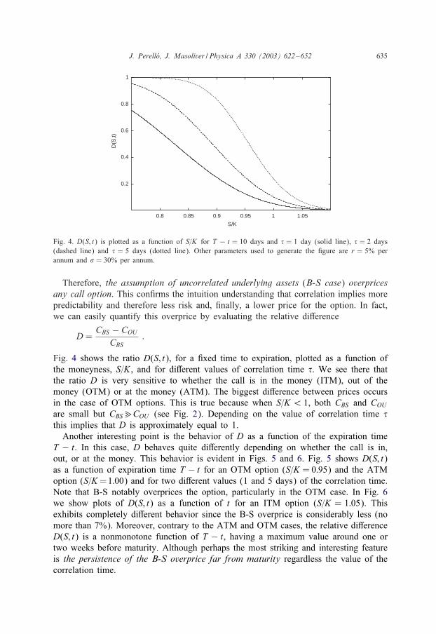
Fig. 4. D(S; t) is plotted as a function of S=K for T − t = 10 days and � = 1 day (solid line), � = 2 days(dashed line) and � = 5 days (dotted line). Other parameters used to generate the /gure are r = 5% perannum and � = 30% per annum.

Therefore, the assumption of uncorrelated underlying assets (B-S case) overpricesany call option. This con/rms the intuition understanding that correlation implies morepredictability and therefore less risk and, /nally, a lower price for the option. In fact,we can easily quantify this overprice by evaluating the relative di4erence

D =CBS − COU

CBS:

Fig. 4 shows the ratio D(S; t), for a /xed time to expiration, plotted as a function ofthe moneyness, S=K , and for di4erent values of correlation time �. We see there thatthe ratio D is very sensitive to whether the call is in the money (ITM), out of themoney (OTM) or at the money (ATM). The biggest di4erence between prices occursin the case of OTM options. This is true because when S=K ¡ 1, both CBS and COU

are small but CBS�COU (see Fig. 2). Depending on the value of correlation time �this implies that D is approximately equal to 1.

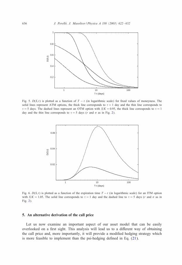
Another interesting point is the behavior of D as a function of the expiration timeT − t. In this case, D behaves quite di4erently depending on whether the call is in,out, or at the money. This behavior is evident in Figs. 5 and 6. Fig. 5 shows D(S; t)as a function of expiration time T − t for an OTM option (S=K = 0:95) and the ATMoption (S=K =1:00) and for two di4erent values (1 and 5 days) of the correlation time.Note that B-S notably overprices the option, particularly in the OTM case. In Fig. 6we show plots of D(S; t) as a function of t for an ITM option (S=K = 1:05). Thisexhibits completely di4erent behavior since the B-S overprice is considerably less (nomore than 7%). Moreover, contrary to the ATM and OTM cases, the relative di4erenceD(S; t) is a nonmonotone function of T − t, having a maximum value around one ortwo weeks before maturity. Although perhaps the most striking and interesting featureis the persistence of the B-S overprice far from maturity regardless the value of thecorrelation time.


0.2

0.4

0.6

0.8

1

1 10 100

D(S

,t)

T-t (days)

Fig. 5. D(S; t) is plotted as a function of T − t (in logarithmic scale) for /xed values of moneyness. Thesolid lines represent ATM options, the thick line corresponds to � = 1 day and the thin line corresponds to� = 5 days. The dashed lines represent an OTM option with S=K = 0:95, the thick line corresponds to � = 1day and the thin line corresponds to � = 5 days (r and � as in Fig. 2).

0.02

0.04

0.06

1 10 100

D(S

,t)

T-t (days)

Fig. 6. D(S; t) is plotted as a function of the expiration time T − t (in logarithmic scale) for an ITM optionwith S=K = 1:05. The solid line corresponds to � = 1 day and the dashed line to � = 5 days (r and � as inFig. 2).

5. An alternative derivation of the call price

Let us now examine an important aspect of our asset model that can be easilyoverlooked on a /rst sight. This analysis will lead us to a di4erent way of obtainingthe call price and, more importantly, it will provide a modi/ed hedging strategy whichis more feasible to implement than the psi-hedging de/ned in Eq. (21).


We start by noting that one might argue that the O-U process (2)–(3) is an inade-quate asset model since the share price S(t) given by Eq. (2) is a continuous randomprocess with bounded variations. As Harrison et al. [29] showed, continuous processeswith bounded variations allow arbitrage opportunities and this is an undesirable fea-ture for obtaining a fair price. Thus, for instance, arbitrage would be possible withina portfolio containing bonds and stock whose strategy at time t is buying (or selling)stock shares when � + V (t) is greater (or lower) than the risk-free bond rate [29].

In our case, however, the problem is that in the practice the return velocity V (t) isnontradable and its evolution is ignored. In other words, in real markets the observedasset dynamics does not show any trace of the velocity variable. Indeed, knowing V (t)would imply knowing the value of the return R(t) at two di4erent times, since

V (t) = lim+→0+

R(t) − R(t − +)+

− � :

Obviously, this operation is not performed by traders who only manage portfolios attime t based on prices at t and not at any earlier time.

This feature allows us to perform a projection of the two-dimensional di4usion pro-cess (S(t); V (t)) onto a one-dimensional equivalent process VS(t) independent of thevelocity V :

(S(t); V (t)) → VS(t) :

We will show next that the projected process VS(t) is equal to the actual price S(t) inmean square sense and that VS(t) obeys the following one-dimensional SDE

d VS(t)VS(t)

= [� + �(T − t)=2] dt +√

�(T − t) dW (t) ; (42)

where �(t) is given by Eq. (10), and the dot denotes time derivative. Therefore, theprice given by Eq. (42) is driven by a noise of unbounded variation, the Wienerprocess, and the Harrison et al. [29] results do not apply. In consequence, the O-Uprojected process is still a suitable starting point for option pricing since it does notpermit arbitrage.

5.1. The projected process

We /rst note that the dynamics of the return R(t) = ln[S(t)=S0] is given by thesecond-order SDE (6) which includes the stochastic evolution of the velocity V (t):

�d2R(t)

dt2+

dR(t)dt

= � + �dW (t)

dt:

Let us now obtain a /rst-order SDE describing the price dynamics when velocity V (t)has been eliminated (see Eq. (50) below).

The starting point of our derivation is the marginal conditional density of the returnp(R; t|R0; t0;V0). This density is given by Eq. (A.14) of Appendix A and when t0 �= 0it reads

p(R; t|R0; t0;V0) =1√

2�K11(t − t0)exp

{− [R− R0 − m(t − t0; V0)]2

2K11(t − t0)

}; (43)


where m(t; V0) and K11(t) are given by Eqs. (7) and (8). Note that the conditionaldensity p(R; t|R0; t0;V0) is the solution of the following partial di4erential equation

9p9t0

= −[� + V0e−(t−t0)=�]9p9R0

− �2

2[1 − e−(t−t0)=�]2

92p9R2

0; (44)

with the /nal condition p(R; t|R0; t;V0) = �(R − R0). Observe that the Eq. (44) is abackward Fokker-Planck equation whose drift, �+V0 exp[−(t−t0)=�], and di4usion co-e*cient, 1

2�2[1−exp[−(t−t0)=�]]2, are both functions of t−t0. As is well-known, there

exists a direct relation between the Fokker-Planck equation and the SDE governing theprocess [19]. In our case, the corresponding SDE is

dR(t0) = [� + V0e−(t−t0)=�] dt0 + �[1 − e−(t−t0)=�] dW (t0) ; (45)

and its formal solution is

R(t) = R(t0) + �(t − t0) + V0�[1 − e−(t−t0)=�] + �∫ t

t0[1 − e−(t−t1)=�] dW (t1) :

(46)

To avoid confusion, let VR(t) be the solution of the /rst-order SDE (45), i.e., VR(t) is theprojected process given by Eq. (46). And let R(t) be the solution of the second-orderSDE (6) where the dynamics of the velocity is still taken into account. Thus, R(t) isexplicitly given by Eq. (A.1) of Appendix A.

We will now prove that VR(t) and R(t) are equal in mean square sense. That is:

〈(R(t) − VR(t))2〉 = 0; for any time t : (47)

In e4ect, from Eq. (46) and assuming, without loss of generality, that t0 = 0 andVR(t0) = 0 we have

VR(t) = �t + V0�(1 − e−t=�) +∫ t

0[1 − e−(t−t1)=�]�(t1) dt1 ; (48)

where �(t1) = dW (t1)=dt1 is the Gaussian white noise. On the other hand, fromEq. (A.1) we write

R(t) = �t + V0�(1 − e−t=�) +��

∫ t

0dt′

∫ t′

0e−(t′−t′′)=��(t′′) dt′′ : (49)

Therefore,

〈(R(t) − VR(t))2〉= 2K11(t) − 2�2

�

∫ t

0dt′

∫ t′

0dt′′e−(t′−t′′)=�

×∫ t

0dt1[1 − e−(t−t1)=�]〈�(t1)�(t′′)〉 ;

where K11(t) is given by Eq. (8). Taking into account that

〈�(t1)�(t′′)〉 = �(t1 − t′′) ;


we have

〈(R(t) − VR(t))2〉 = 2K11(t) − 2�2

�

∫ t

0dt′

∫ t′

0dt′′e−(t′−t′′)=�[1 − e−(t−t′′)=�] :

However, (see Eq. (8))

�2

�

∫ t

0dt′

∫ t′

0dt′′e−(t′−t′′)=�[1 − e−(t−t′′)=�] = K11(t) :

Hence,

〈(R(t) − VR(t))2〉 = 0 ;

and R(t) is equal to VR(t) in mean square sense.As we have mentioned, we are mainly interested in representing the asset dynamics

when the initial velocity V0 is random and distributed according to the stationarypdf (9). In such a case, the SDE for R(t) reads 4

dR(t) = � dt +√

�(T − t) dW (t) ; (50)

where �(t) is given by Eq. (10) and the dot denotes time derivative, that is

�(t) = �2(1 − e−t=�) : (51)

We /nally obtain the corresponding SDE for the stock price de/ned as S = S0eR. Wesubstitute Eq. (50) in the Taylor expansion

dS(R) = SR dR +12SRR dR2 + · · · ;

neglecting orders higher than dt and taking into account that dR2 = �(T − t) dt (inmean square sense), we get

dS(t)S(t)

= [� + �(T − t)=2] dt +√

�(T − t) dW (t) ; (52)

which is Eq. (42). In this way, we have projected the two-dimensional O-U process(S; V ) onto a one-dimensional price process which is a Wiener process with timevarying drift and volatility. We also note that we need to specify the /nal conditionof the process because the volatility

√� is a function of the time to maturity T − t,

and this implies that the projected asset model depends on each particular contract.

5.2. The projected process and the B-S portfolio

Assuming that the e4ective one-dimensional price dynamics is given by Eq. (52),it is quite straightforward to derive the European call option price within the originalB-S method and using the standard portfolio containing shares, bonds and calls. Indeed,proceeding in the same way as in Section 3.1 we get[

Ct +12�(T − t)S2CSS + r�S − rC

]dt = [�− CS ] dS :

4 Since R(t) and VR(t) are equal in mean square sense we will drop the bar on VR as long as there is noconfusion. Thus, we will use R for the projected process as well.


Now the B-S delta hedging, � = CS , removes any random uncertainty in the optionprice. The partial di4erential equation for C(S; t) then reads

Ct = rC − rSCS − 12�(T − t)S2CSS : (53)

We note that the delta hedging is able to remove risk because we have projectedthe two-dimensional SDE (2)–(3) onto the one-dimensional process. In this way, wedirectly relate the di4erential of the stock dS(t) to the random @uctuations of theWiener process dW (t) (see Eq. (42)). Recall that, without this projection, the B-Shedging is useless since, as explained in Section 3.1, the random @uctuations persistin the B-S portfolio.

For the European call, Eq. (53) has to be solved with the “/nal condition” at maturitytime which is C(S; T )=max[S(T )−K; 0]. The solution to Eq. (53) subject to Eq. (26)is a type of solution perfectly known in the literature [27]. The /nal price is

COU (S; t) = SN (dOU1 ) − Ke−r(T−t)N (dOU

2 ) ;

where N (z) is the probability integral, and

dOU1 =

ln (S=K) + r(T − t) + �(T − t)=2√�(T − t)

;

dOU2 = dOU

1 −√

�(T − t) ;

with �(t) given by Eq. (10). Thus the B-S method applied to the projected processresults in the same price as the one derived from the modi/ed (see Eq. (35)). Therefore,the two approaches are consistent.

5.3. The projected process and the modi7ed portfolio

Suppose we start from the modi/ed portfolio having bonds, calls and secondary calls(cf. Eq. (18)) but now assuming that the share price is given by the projected process(52) instead of the two-dimensional O-U process (2)–(3). In this case, one can obtainthe same option price as before (cf. Eq. (35)) but with a modi/ed hedging strategygiven by the following function

(S; t) =CS

C′S: (54)

Let us prove this. We start from Eq. (19):

dC = � dB + dC′ ;

Now, instead of Eq. (20) we have (see Ito lemma given by Eq. (B.4) of Appendix B)[(Ct +

12�(T − t)CSS − rC

)−

(C′

t +12�(T − t)C′

SS − rC′)]

dt

=( C′S − CS) dS ; (55)


and removal of risk implies Eq. (54). The psi hedging given by Eq. (54) is evidentlyrelated to the psi hedging de/ned in Eq. (21) although now it is represented in termsof the /nal price COU (S; t) instead of the intermediate price C(S; V; t). Clearly psihedging in terms of C(S; V; t) requires the knowledge of the return velocity V . Inpractice, this is impossible since, as we have mentioned above, velocity is nontradableand its evolution is ignored. Therefore, in order to implement psi hedging based onC(S; V; t) we should eliminate the velocity of Eq. (21) by means of some averagingprocedure. In consequence psi hedging in terms of COU (S; t) is easier to implement inpractice than the psi hedging based on C(S; V; t).

Substituting Eq. (54) into Eq. (55) and reasoning along the same line as above (seeEqs. (22) and (23)) we obtain

Ct +12�(T − t)S2CSS − rC = !CS ; (56)

where !=!(S; t) is the “risk premium” for the e4ective process which is now obviouslyindependent of the velocity V .

We next apply the Ito lemma, as expressed by Eq. (B.4) of Appendix B, to C(S; t)with the result

dC(S; t) = CS dS + Ct dt +12�(T − t)S2CSS dt ;

which, after using Eqs. (42) and (56), reads

dC(S; t) ={rC +

[!S

+ � +12�(T − t)

]SCS

}dt +

√�(T − t)SCS dW (t) :

(57)

Hence, the conditional expected value of dC is

〈dC|C〉 ={rC +

[!S

+ � +12�(T − t)

]SCS

}dt ; (58)

but the statistical absence of arbitrage implies that 〈dC|C〉 = rC dt. Therefore, weconclude that

! = −S[� +

12�(T − t)

]; (59)

and Eq. (56) reads

Ct +12�(T − t)S2CSS − rC +

[� +

12�(T − t)

]SCS = 0 ;

Finally, again, the absence of arbitrage opportunities requires the replacement (seeEq. (30))

� + �(T − t)=2 → r :

Thus, the option price equation is

Ct = rC − rSCS − 12�(T − t)S2CSS ; (60)


which agrees with Eq. (53). Note that both procedures, the original B-S method pre-sented in previous section and our method, result in the same partial di4erential equa-tion for the call price. However, each method uses a di4erent hedging strategy becausethey start from a di4erent portfolio. In the following section we deeper analyze thesedi4erent hedging strategies.

6. Greeks and hedging

We brie@y derive the Greeks for the O-U case. Since the O-U call price has thesame functional form as the B-S price but replaces �2(T − t) by �(T − t), the O-UGreeks will have the same functional form as B-S Greeks with the same replacementexcept for Vega, V=9C=9�, and , = 9C=9t. Thus, for � = 9C=9S, - = 92C=9S2, and. = 9C=9r, we have [27]

�OU = N (dOU1 ) ; -OU =

e−(dOU1 )2=2

S√

2��(T − t); .OU = K(T − t)e−r(T−t)N (dOU

2 ) :

(61)

Since dOU1;2 ¿dBS

1;2 for all S and t and N (z) is a monotone increasing function, we seethat �OU ¿ �BS and .OU ¿ .BS . Hence, the O-U call price is more sensitive to changesin stock price and interest rate than the B-S price.

On the other hand, from Eq. (35) and taking into account the identity

SN ′(d1) − Ke−r(T−t)N ′(d2) = 0 ; (62)

we have

VOU = (S=�)[�(T − t)=2�]1=2e−(dOU1 )2=2 ; (63)

and

,OU = −Ke−r(T−t)

[rN (dOU

2 ) +�2(1 − e−(T−t)=�)

2√

2��(T − t)e−(dOU

2 )2=2

]: (64)

Since dOU1 ¿dBS

1 , one can easily see that VOU 6VBS for all values of S=K , T − tand �. Thus our correlated call price is less sensitive to any change of underlyingvolatility � than is the B-S price.

We conclude with the psi hedging. For the two-dimensional O-U case the hedgingstrategy is given by the function (S; V; t) specifying the number of secondary callsto be hold. However, the hedging given by Eq. (21) depends on the velocity V andis not expressed in terms of the /nal call price COU = C(S; t). As we have shownin Section 5.3, psi hedging in terms of COU can only be derived from the e4ectiveone-dimensional process (42). In this case, the removal of the randomness comingfrom dS implies that hedging is given by Eq. (54). Since CS = �OU , we see from


0.2

0.4

0.6

0.8

0.7 0.8 0.9 1 1.1 1.2

hedg

ing

moneyness

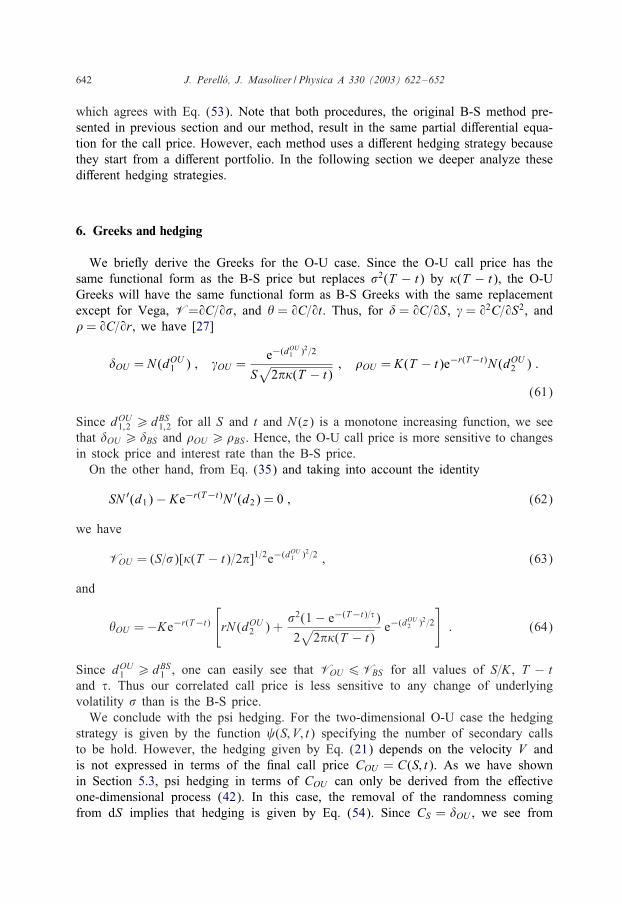
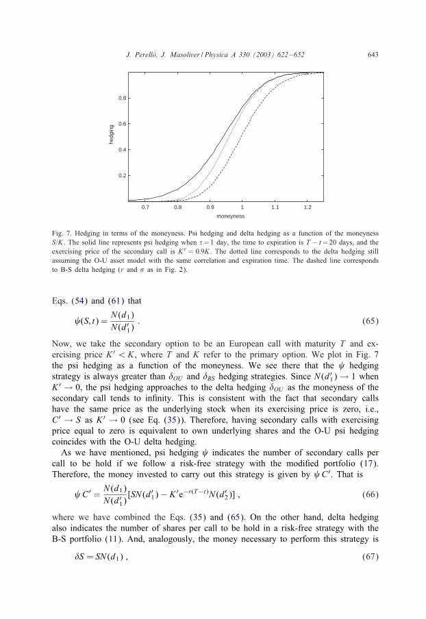
Fig. 7. Hedging in terms of the moneyness. Psi hedging and delta hedging as a function of the moneynessS=K . The solid line represents psi hedging when �=1 day, the time to expiration is T − t =20 days, and theexercising price of the secondary call is K ′ = 0:9K . The dotted line corresponds to the delta hedging stillassuming the O-U asset model with the same correlation and expiration time. The dashed line correspondsto B-S delta hedging (r and � as in Fig. 2).

Eqs. (54) and (61) that

(S; t) =N (d1)N (d′

1): (65)

Now, we take the secondary option to be an European call with maturity T and ex-ercising price K ′ ¡K , where T and K refer to the primary option. We plot in Fig. 7the psi hedging as a function of the moneyness. We see there that the hedgingstrategy is always greater than �OU and �BS hedging strategies. Since N (d′

1) → 1 whenK ′ → 0, the psi hedging approaches to the delta hedging �OU as the moneyness of thesecondary call tends to in/nity. This is consistent with the fact that secondary callshave the same price as the underlying stock when its exercising price is zero, i.e.,C′ → S as K ′ → 0 (see Eq. (35)). Therefore, having secondary calls with exercisingprice equal to zero is equivalent to own underlying shares and the O-U psi hedgingcoincides with the O-U delta hedging.

As we have mentioned, psi hedging indicates the number of secondary calls percall to be hold if we follow a risk-free strategy with the modi/ed portfolio (17).Therefore, the money invested to carry out this strategy is given by C′. That is

C′ =N (d1)N (d′

1)[SN (d′

1) − K ′e−r(T−t)N (d′2)] ; (66)

where we have combined the Eqs. (35) and (65). On the other hand, delta hedgingalso indicates the number of shares per call to be hold in a risk-free strategy with theB-S portfolio (11). And, analogously, the money necessary to perform this strategy is

�S = SN (d1) ; (67)


0.4

0.8

1.2

0.8 1 1.2 1.4

rela

tive

hedg

ing

cost

moneyness

Fig. 8. Relative hedging costs C′=K and �S=K as a function of the moneyness S=K . The solid line representpsi hedging cost when � = 1 day, the time to expiration is T − t = 20 days, and the exercising price of thesecondary call is K ′ =0:9K . The dotted line corresponds to the delta hedging with �=1 day and T − t =20days (r and � as in Fig. 2).

where � is given by Eq. (61). We compare these quantities in order to know whichhedging is cheaper for the investor. From Eqs. (66) and (67), we see

C′

�S= 1 − K ′e−r(T−t)N (d′

2)SN (d′

1);

but 5

06K ′e−r(T−t)N (d′

2)SN (d′

1)6 1 :

Therefore, C′ ¡�S and psi hedging is always less expensive than delta hedging. Notethat when K ′ → 0 both strategies have the same cost. In Fig. 8 we plot, as a functionof moneyness, the relative psi hedging cost, C′=K , along with the relative deltahedging cost, �S=K . We see there that psi hedging is considerably less expensive thandelta hedging and this di4erence increases with moneyness. Indeed, for an ATM call(S=K=1:00) and with parameter values as that of Fig. 8, delta hedging is approximately800% more expensive than psi hedging.

Combining Eqs. (38), (54) and (62) one can easily show that when � = 0 the O-Upsi hedging is BS = N (dBS

1 )=N (dBS′1 ), 6 where the prime refers to the secondary call.

Since � = CS = N (d1), we have

BS =�BS

�′BS:

5 This is straightforward to prove from Eq. (66) since C′¿ 0.6 We use the subscript BS in BS to indicate that this hedging refers to an uncorrelated stock (� = 0), as

in the B-S world.


Finally, for the secondary call, whose exercising price goes to zero, �′BS → 1 and,again, B-S psi hedging and B-S delta hedging coincide.

7. Conclusions

We have developed option pricing with perfect hedging in an ine*cient marketmodel. The ine*ciency of the market is related to the fact that the underlying pricevariations are autocorrelated over an arbitrary time period �. In order to take thesecorrelations into account we have modelled the underlying price S(t) as a singulardi4usion process in two dimensions (O-U process) instead of the standard assumptionthat S(t) is a one-dimensional di4usion given by the geometric Brownian motion withconstant volatility.

The option pricing method has been developed by keeping perfect hedging with ariskless strategy which /nally results in a closed and exact expression for the Europeancall. Our pricing formula has the same functional form as the B-S price but replacesthe variance of the Wiener process by the variance of the O-U process. The O-Uvariance, �(t), is smaller than the B-S variance, �2t, which implies that the equivalentvolatility in the O-U case is lower than B-S volatility. 7 But less volatility implies alower option price. We have indeed proved that the B-S call price is always greaterthan the O-U price. In other words, the assumption of uncorrelated assets overpricesthe European call. This agrees with the fact that correlation, which can be regarded asa form of predictability, implies less risk and therefore a lower price for the option.We have quanti/ed this overprice and showed that B-S formula notably overpricesoptions and, more strikingly, that the overprice persists for a long time regardless ofthe strength of correlations. We have also analyzed the sensitivity of the O-U price toseveral conditions. Thus we have proved that while COU is more sensitive to changesin the interest rate and stock price than CBS , it is also less sensitive to any change ofthe volatility. The practical consequences of this are nontrivial.

The option price and the hedging strategy have been obtained using two di4erentapproaches. A straightforward way of getting the call price is by means of a projectiononto a one-dimensional process with a time-varying volatility and then using the stan-dard B-S procedure. Another way of obtaining the option price starts with the completetwo-dimensional O-U process (2)–(3). This is a longer procedure but opens the door toa new hedging strategy: the psi hedging. We have therefore two ways of achieving theperfect hedging: the usual one consisting in holding underlying assets (delta hedging),and the second one which uses secondary calls 8 instead of assets (psi hedging). Wehave shown that this last strategy can be considerable less expensive than the deltahedging and can avoid a possible lack of liquidity of underlying shares. Finally, the

7 Since the volatility � is the square root of the variance per unit time, one can de/ne, in the O-U case,an equivalent volatility by �OU =

√�(t), where the dot denotes time derivative. From Eq. (10) we see that

�OU =� =√

1 − e−t=�6 1.8 The construction of the portfolio with secondary calls is one simple way of proceeding. Obviously, any

other secondary derivative on the same asset would serve.


proportion of secondary calls to be held, i.e., the psi hedging, converges towards O-Udelta hedging when the exercising price of the secondary call tends to zero.

In practice our method of valuation requires the estimate of one more parameter, thecorrelation time, than in the B-S Wiener case. Assuming that the underlying asset isdriven by O-U noise one can /nd an estimate for the correlation time � by evaluatingthe variance �(t) of the asset return. Once one has an estimate of this variance thecorrelation time is given in Eq. (10).

Before ending this paper, we consider two possible extensions. There is an interestingwork by Bouchaud et al. [30] that also deals with correlation e4ects in option pricing.Their paper is focussed on colored and not necessarily Gaussian random noises but ina discontinuous time setting. In such a case, they use di4erent formalism than that ofthe Black-Scholes method [10]. This is an interesting approach in case one wants togo beyond the Gaussianity in the market modelisation while keeping the presence ofcorrelations. Finally, another interesting extension of the valuation method presented isto the American option. Although this case is more involved, one is probably able toobtain, at least an approximate or a numerical result using /rst passage times. In anycase we believe that the e4ects of autocorrelations on the valuation of an Americanoption will be even more critical than for the European call. This case is under presentinvestigation.

Acknowledgements

The authors acknowledge helpful comments and discussions with Alan McKane,Miquel Montero, Josep M. PorrYa and Jaume Puig. We are particularly grateful toSantiago Carrillo and George H. Weiss for their many suggestions to improve themanuscript. This work has been supported in part by Direcci#on General de Proyectosde Investigaci#on under contract No. BFM2000-0795, and by Generalitat de Catalunyaunder contract No. 2000 SGR-00023.

Appendix A. Mathematical properties of the model

We present some of the most important properties of the model given by the pairof stochastic equations in Eqs. (4) and (5). Their formal solutions are

V (t) = V0e−(t−t0)=� +��

∫ t

t0e−(t−t′)=� dW (t′) ;

and

R(t) = �(t − t0) + V0�(1 − e−(t−t0)=�) +��

∫ t

t0dt′

∫ t′

t0e−(t′−t′′)=� dW (t′′) ;

(A.1)

where we have assumed that the process begun at time t0 with initial velocity V0 andreturn R0 = 0. The return R(t) has the following conditional mean value

〈R(t)|V0〉 = �(t − t0) + �(1 − e−(t−t0)=�)V0 ;


and variance

Var[R(t)|V0] = �2[(t − t0) − 2�(1 − e−(t−t0)=�) +

�2(1 − e−2(t−t0)=�)

]:

Since (R(t); V (t)) is a di4usion process in two dimensions, its joint density p(R; V; t)satis/es the following Fokker-Planck equation [19]

pt = −(� + V )pR +V�

pV +�2

2�2 pVV : (A.2)

This is to be solved subject to the initial conditions R(t0) = 0 and V (t0) = V0, that is

p(R; V; t0|V0; t0) = �(R)�(V − V0) : (A.3)

A /rst step towards solving the problem (A.2) and (A.3) is the de/nition of the jointFourier transform

p((; "; t) =∫ ∞

−∞dRei(R

∫ ∞

−∞dV ei"Vp(R; V; t) :

Then problem (A.2) and (A.3) becomes

9t p = i(�p + ((− "=�)(9"p− (�2=2�2)"2p ; (A.4)

p((; "; t = 0) = ei"V0 : (A.5)

We look for a solution of the form

p((; "; t)=exp{i[(m1(t)+"m2(t)]}exp{−[K11(t)(2 +K12(t)("+K22(t)"2]=2} ;(A.6)

where mi(t) and Kij(t) are functions to be determined. We substitute Eq. (A.6) into(A.4) and identify term by term. We have

m1 = � + m2; m2 = −m2=� ;

K22 + (2=�)K22 = �2�2; K12 + (1=�)K12 = 2K22(t); K11 = 2K12 ;

with initial conditions, according to Eqs. (A.5) and (A.6), given by

m2(0) = V0; m1(0) = Kij(0) = 0 (i; j = 1; 2) :

The solution reads

m1(t) = �t + V0�(1 − e−t=�); m2(t) = V0e−t=� ;

and Kij(t) are given by

K11(t) = �2[t − 2�(1 − e−t=�) +

�2(1 − e−2t=�)

]; (A.7)

K12(t) =�2

2(1 − e−t=�)2; K22(t) =

�2

2�(1 − e−2t=�) : (A.8)


The inverse Fourier transform of Eq. (A.6) yields the Gaussian density

p(R; V; t|V0; t0)

=1

2�√

det[K (t − t0)]exp

{− (V − V0e−(t−t0)=�)2

2K22(t − t0)

− [K22(t − t0)(R− m(t − t0; V0)) − K11(t − t0)(V − V0e−(t−t0)=�)]2

2K22(t − t0) det[K (t − t0)]

};

(A.9)

where

det[K (t)] ≡ K11(t)K22(t) − K212(t) : (A.10)

and

m(t; V0) = �t + V0�(1 − e−t=�) : (A.11)

Notice that the joint density (A.9) is a function of the time di4erences t − t0 where t0is the initial observation time, so that the two-dimensional di4usion (S(t); V (t)) is atime homogeneous process and, without loss of generality, we may assume that t0 =0.

The marginal pdf of the velocity V (t),

p(V; t|V0) =∫ ∞

−∞p(R; V; t|V0) dR ;

is

p(V; t|V0) =1√

2�K22(t)exp

[− (V − V0e−t=�)2

2K22(t)

]: (A.12)

In the stationary regime (t → ∞) we /nd a normal density independent of the initialvelocity:

pst(V ) =1√

�(�2=�)e−�V 2=�2

: (A.13)

Analogously, the marginal density of the return R(t),

p(R; t|V0) =∫ ∞

−∞p(R; V; t|V0) dV ;

is

p(R; t|V0) =1√

2�K11(t)exp

{− [R− m(t; V0)]2

2K11(t)

}: (A.14)

If we assume that the initial velocity V0=V (0) is a random variable distributed accord-ing to the pdf in Eq. (A.13). We can therefore average the above densities to obtaina pdf independent of V0. That is,

p(R; V; t) =∫ ∞

−∞p(R; V; t|V0)pst(V0) dV0 ;


and similarly for the marginal pdf’s p(R; t) and p(V; t). Since we are mainly interestedon the marginal distribution of the return we will give its explicit expression. Thus,from Eqs. (A.13) and (A.14) we have

p(R; t) =1√

2��(t)exp

[− (R− �t)2

2�(t)

]; (A.15)

where �(t) is given by Eq. (10).

Appendix B. The Ito formula for processes driven by O-U noise

In this Appendix we generalize the Ito formula for processes driven by Ornstein-Uhlenbeck noise. This is applied to the share price S(t) which is governed by the pairof stochastic equations (2) and (3)

dS(t) = S(� + V ) dt; dV (t) = −V�

dt +��

dW : (B.1)

Consider a generic function f(S; V; t) which depends on all of the variables that char-acterize the underlying asset. The di4erential of f(S; V; t) is de/ned by

df(S; V; t) ≡ f(S(t + dt); V (t + dt); t + dt) − f(S(t); V (t); t) : (B.2)

But the Taylor expansion of (B.2) yields

df(S; V; t)=fS dS+fV dV +ft dt+ 12 fSS dS2 + 1

2 fVV dV 2 +fSVdSdV + · · · ;(B.3)

where the expansion also involves higher order di4erentials such as (dt)2, (dS)3, (dV )3,etc. However, the di4erential of the Wiener process, dW , satis/es the well-knownproperty, in the mean-square sense, dW (t)2 =dt [19]. And from the pair of Eqs. (B.1)we then see that dS2 is of order dt2 while dV 2 is of order dt and dS dV is of orderdt3=2. Therefore, up to order dt, Eq. (B.3) reads

df(S; V; t) = fS dS + fV dV + ft dt +�2

2�2 fVV dt ;

which is the Ito formula for our singular two-dimensional process (2) and (3).Moreover, we can also give the di4erential of a generic function f(S; t) when un-

derlying obeys SDE

dS(t)S(t)

= [� + �(T − t)=2] dt +√

�(T − t) dW (t) ;

which is Eq. (42). In this case, we have

df(S; t) = fS dS + ft dt +12�(T − t)S2fSS dt ; (B.4)

where again we have neglected higher order contributions than dt.


Appendix C. A derivation of the risk premium

We proceed to /nd a closed expression for the arbitrary function !(S; V; t) thatappears in Eq. (23). The call price C is a function of S; V , and t. We now considerthis function taking into account that S = S(t) and V = V (t) follow Eqs. (2) and (3),respectively. This therefore allows us to evaluate the random di4erential dC using theIto lemma, as a result we /nd that

dC =[Ct + (� + V )SCS +

�2

2�CVV

]dt + CV dV :

After using Eqs. (23) and (3), we have

dC =[rC +

(!− V

�

)CV

]dt +

��CV dW : (C.1)

The expected value of dC, on the assumption that C(t) = C is known, reads

〈dC|C〉 =[rC +

(!− V

�

)CV

]dt : (C.2)

We claim that this average must grow at the same rate as the risk-free bond:

〈dC|C〉 = rC dt ; (C.3)

This assumption says that the asset grows in average as the risk-free bond [27] andwe thus assert that the asset has no statistical arbitrage opportunities.

The substitution of Eq. (C.3) into Eq. (C.2) yields the following expression for therisk premium !(S; V; t):

! =V�

: (C.4)

Appendix D. Solution to the problem in Eqs. (25) and (26)

We will solve Eq. (25) subject to the /nal condition in Eq. (26). De/ne a newindependent variable Z

S = eZ ;

where the domain of Z is unrestricted. The problem posed in Eqs. (25) and (26) nowreads

Ct = rC − (� + V )CZ +V�CV − �2

2�CVV ;

C(Z; V; T ) = max[eZ − K; 0] :

The solution to this problem can be written in the form

C(Z; V; t) =∫ ∞

−∞dZ ′

∫ ∞

−∞dV ′max[eZ

′ − K]G(Z; V; t|Z ′; V ′; T ) ; (D.1)


where G(Z; V; t|Z ′; V ′; T ) is the Green function for the problem [28], i.e., G(Z; V; t|Z ′;V ′; T ) is the solution to

Gt = rG − (� + V )GZ +V�

GV − �2

2�GVV ; (D.2)

with the /nal condition

G(Z; V; T |Z ′; V ′; T ) = �(Z − Z ′)�(V − V ′) ; (D.3)

where �(X − X ′) is the Dirac delta function. De/ne VG = e−rtG, then the /nal-valueproblem in Eqs. (D.2) and (D.3) reads

VGt = −(� + V ) VGZ +V�

VGV − �2

2�VGVV ; (D.4)

VG(Z; V; T |Z ′; V ′; T ) = e−rT �(Z − Z ′)�(V − V ′) : (D.5)

Note that Eq. (D.4) is the backward equation corresponding to Eq. (A.2). Therefore,Eq. (A.9) permits us to write the solution to the problem posed in Eqs. (D.4) and(D.5) [19]. This solution implies that G is

G(Z; V; t|Z ′; V ′; T )

=1

2�√

det[K (T − t)]exp

{−r(T − t) − [V ′ − V e−(T−t)=�]2

2K22(T − t)

− [K22(T − t)(Z ′ − Z + m(T − t; V )) − K11(T − t)(V ′ − V e−(T−t)=�)]2

2K22(T − t)det[K (T − t)]

};

(D.6)

where det[K (t)], Kij(t), and m(t; V ) are de/ned in Eqs. (A.10) and (A.11).Substituting Eq. (D.6) into Eq. (D.1) and /nally reverting to the original variables

we obtain Eq. (27) with

z1 =ln(S=K) + m(T − t; V ) + K11(T − t)√

K11(T − t); z2 = z1 −

√K11(T − t) : (D.7)

Finally it can be shown, after some lengthy but simple manipulations, that the functionsVz1;2 = Vz1;2(S; T − t) appearing in the averaged price VC(S; t), Eq. (29), are given by

Vz1 =ln(S=K) + �(T − t) + �(T − t)√

�(T − t); Vz2 = Vz1 −

√�(T − t) ; (D.8)

where �(t) is given in Eq. (10).

References

[1] F. Black, M. Scholes, J. Pol. Econ. 81 (1973) 637–659.[2] R.C. Merton, Bell J. Econ. Manage. Sci. 4 (1973) 141–183.[3] W.F. Sharpe, J. Fin. 19 (1964) 425–442.


[4] J.C. Cox, S.A. Ross, J. Financial Econ. 3 (1976) 145–166.[5] E.F. Fama, J. Bus. 38 (1965) 34–105.[6] H. Markowitz, J. Finance 7 (1952) 77–91.[7] R.C. Merton, J. Financial Econ. 3 (1976) 125–144.[8] E.F. Fama, J. Finance 46 (1976) 1575–1617;

S.J. Grossman, J.E. Stiglitz, Am. Econom. Rev. 70 (1980) 222–227.[9] S. Figlewski, J. Finance 64 (1989) 1289–1311;

E. Aurell, R. Baviera, O. Hammarlid, M. Serva, A. Vulpiani, Int. J. Theo. Appl. Finance 3 (2000)1–24.

[10] J.-P. Bouchaud, M. Potters, Theory of Financial Risks, Cambridge University Press, Cambridge, UK,2000.

[11] G.E. Uhlenbeck, L.S. Ornstein, Phys. Rev. 31 (1930) 823–841.[12] J.L. Doob, Ann. Math. 43 (1942) 351–369.[13] E.M. Stein, J.C. Stein, Rev. Financial Stud. 4 (1991) 727–752.[14] J. Masoliver, J. Perell#o, Int. J. Theo. Appl. Fin. 5 (2002) 541;

J. Perell#o, J. Masoliver, Phys. Rev. E 67 (2003) 037102 (4 pages).[15] W. Breen, R. Jagannathan, J. Finance 44 (1989) 1177–1189;

J. Campbell, Y. Hamao, J. Finance 47 (1992) 43–70.[16] A.W. Lo, J. Wang, J. Finance 50 (1995) 87–129.[17] J. Perell#o, J. Masoliver, Physica A 308 (2002) 420–442;

J. Perell#o, J. Masoliver, Physica A 314 (2002) 736–742.[18] Y.Z. Bergman, B.D. Grundy, Z. Wiener, J. Finance 42 (1987) 281–300.[19] C.W. Gardiner, Handbook of Stochastic Methods, Springer, New York, 1985.[20] M.J. Lighthill, An Introduction to Fourier Analysis and Generalized Functions, Cambridge University

Press, Cambridge, UK, 1958.[21] J.A. Goldstein, Nagoya Mathematical Journal 36 (1969) 27–63;

I.I. Gihman, A.V. Skorohod, Stochastic Di4erential Equations, Springer, New York, 1972.[22] L. Arnold, Stochastic Di4erential Equations: Theory and Applications, Wiley, New York, 1974.[23] R.L. Stratonovich, Topics in the Theory of Random Noise, Gordon and Breach, New York, 1963.[24] R.C. Merton, cited in: P. Samuelson, SIAM Rev. 1 (1973) 34–38.[25] J. Perell#o, J.M. PorrYa, M. Montero, J. Masoliver, Physica A 278 (2000) 260–274.[26] L.O. Scott, J. Financial Quant. Anal. 22 (1987) 419–438.[27] P. Wilmott, Derivatives, Wiley, New York, 1998.[28] T. Mynt-U, Partial Di4erential Equations for Scientists and Engineers, North-Holland, Amsterdam, 1987.[29] J.M. Harrison, R. Pitbladdo, S.M. Schaefer, J. Bus. 57 (1984) 353–365.[30] L. Cornalba, J.-P. Bouchaud, M. Potters, Int. J. Theo. Appl. Fin. 5 (2002) 307–320.

Documents

Option pricing and perfect hedging on correlated stocks