Embed Size (px)
Citation preview

Opting out of the great inflation:German monetary policy afterthe breakdown of Bretton Woods
Andreas Beyer(European Central Bank)
Vitor Gaspar(Banco de Portugal)
Christina Gerberding(Deutsche Bundesbank)
Otmar Issing(Centre for Financial Studies)
Discussion PaperSeries 1: Economic StudiesNo 12/2009Discussion Papers represent the authors’ personal opinions and do not necessarily reflect the views of theDeutsche Bundesbank or its staff.

Editorial Board: Heinz Herrmann Thilo Liebig Karl-Heinz Tödter Deutsche Bundesbank, Wilhelm-Epstein-Strasse 14, 60431 Frankfurt am Main, Postfach 10 06 02, 60006 Frankfurt am Main Tel +49 69 9566-0 Telex within Germany 41227, telex from abroad 414431 Please address all orders in writing to: Deutsche Bundesbank, Press and Public Relations Division, at the above address or via fax +49 69 9566-3077
Internet http://www.bundesbank.de
Reproduction permitted only if source is stated.
ISBN 978-3–86558–518–9 (Printversion) ISBN 978-3–86558–519–6 (Internetversion)

Abstract:
During the turbulent 1970s and 1980s the Bundesbank established an outstanding reputation in the world of central banking. Germany achieved a high degree of domestic stability and provided safe haven for investors in times of turmoil in the international financial system. Eventually the Bundesbank provided the role model for the European Central Bank. Hence, we examine an episode of lasting importance in European monetary history. The purpose of this paper is to highlight how the Bundesbank monetary policy strategy contributed to this success. We analyze the strategy as it was conceived, communicated and refined by the Bundesbank itself. We propose a theoretical framework (following Söderström, 2005) where monetary targeting is interpreted, first and foremost, as a commitment device. In our setting, a monetary target helps anchoring inflation and inflation expectations. We derive an interest rate rule and show empirically that it approximates the way the Bundesbank conducted monetary policy over the period 1975-1998. We compare the Bundesbank's monetary policy rule with those of the FED and of the Bank of England. We find that the Bundesbank's policy reaction function was characterized by strong persistence of policy rates as well as a strong response to deviations of inflation from target and to the activity growth gap. In contrast, the response to the level of the output gap was not significant. In our empirical analysis we use real-time data, as available to policy-makers at the time.
Keywords: E31, E32, E41, E52, E58
JEL-Classification: Inflation, Price Stability, Monetary Policy, Monetary Targeting, Policy Rules

Non technical summary
In the second half of the twentieth century, the German Bundesbank established its
reputation as one of the most successful central banks in the world. Along with the
Swiss National Bank, the Bundesbank was the first central bank to announce and pursue
a strategy based on monetary targets after the breakdown of Bretton Woods. In this
paper, we relate the Bundesbank success in maintaining price stability and in anchoring
inflation expectations to its strategy. We examine the strategy as it was presented,
refined and communicated by the Bundesbank itself. Our goal is to provide a historical
account of the conduct of monetary policy, focusing especially on the first ten years of
monetary targeting, from 1975 until the middle of the 1980s, when price stability was
virtually reached in Germany.
According to the Bundesbank Act, the objective of monetary policy is to safeguard the
currency. The Bundesbank has always interpreted its mandate as giving precedence to
(domestic) price stability. It is, therefore, clear that monetary targets were intermediate
targets. Moreover, the Bundesbank’s operational framework for monetary policy
implementation implied that the first step in the transmission mechanism was the
control over a money market interest rate. Thus, in this paper, we characterize the
Bundesbank’s monetary policy strategy through an interest rate rule in the tradition of
Taylor (1993, 1999), modified to take account of the implications of monetary targeting
for the Bundesbank’s interest rate decisions.
Building on the modified loss function approach (pioneered by Rogoff, 1985), we show
how focusing on money growth helps to bring the conduct of monetary policy closer to
optimal policy under commitment (thereby improving on the outcome under discretion).
It does so by inducing a persistent, history-dependent response of policy rates to
deviations of inflation and output from target. We find that the interest rate rule implied
by our model captures key features of the Bundesbank’s monetary policy actions. In the
modified loss function framework, monetary growth targeting is permanently relevant
and imposes structure on the monetary policy reaction function. Nevertheless, given that
monetary deviations from target have to be traded off against other arguments in the
loss function, frequent deviations from target cannot be excluded. Hence, the operation

of monetary growth targeting as a commitment device is compatible with target misses,
even repeatedly. In practice, the Bundesbank had to account for the determinants of
observed deviations and explain how, in the end, it would deliver on the final goal of
price level stability.
Using real-time data, our main empirical finding is that the Bundesbank response to the
output growth gap was highly significant. Such response is a characteristic of the
conduct of monetary policy under commitment. It is also robust policy against problems
in the measurement of the level of potential output in real time. A similar response to
the growth gap was not present in the reaction function of the Federal Reserve System
during the Burns-Miller period. It does become significant, for the US, in the later
Volcker-Greenspan period. We are able to characterize systematic monetary policy for
Germany and the US. Our empirical findings suggest a much less stable approach in the
UK.

Nicht technische Zusammenfassung
In der zweiten Hälfte des 20. Jahrhunderts begründete die Deutsche Bundesbank ihren
Ruf als eine der erfolgreichsten Zentralbanken weltweit. Neben der Schweizerischen
Nationalbank war die Bundesbank die erste Zentralbank, die nach dem Zusammenbruch
des Bretton-Woods-Systems eine Strategie der Geldmengensteuerung bekannt gab und
verfolgte. In der vorliegenden Arbeit setzen wir den Erfolg der Bundesbank bei der
Gewährleistung der Preisstabilität und der Verankerung der Inflationserwartungen in
Beziehung zu ihrer Strategie. Wir untersuchen diese Strategie in der Form, wie sie von
der Bundesbank formuliert, weiterentwickelt und kommuniziert wurde. Unser Ziel ist
eine historisch akkurate Darstellung der geldpolitischen Entscheidungsfindung, mit
einem besonderen Schwerpunkt auf den ersten zehn Jahren der Geldmengensteuerung,
von 1975 bis Mitte der Achtzigerjahre. Im Laufe dieser Phase wurde in Deutschland
nahezu Preisstabilität erreicht.
Gemäß dem Gesetz über die Deutsche Bundesbank ist die Aufgabe der Geldpolitik die
Währungssicherung. Die Bundesbank hat ihren Auftrag immer dahingehend ausgelegt,
dass sie der (inländischen) Preisstabilität Vorrang gab. Demzufolge ist klar, dass die
Geldmengenziele Zwischenzielgrößen darstellten. Überdies implizierte der
geldpolitische Handlungsrahmen der Bundesbank, dass der erste Schritt im
Transmissionsmechanismus die Kontrolle eines kurzfristigen Zinssatzes am Geldmarkt
war. Deshalb beschreiben wir in dieser Arbeit die Geldpolitik der Bundesbank mithilfe
einer Zinsregel in der Tradition Taylors (1993, 1999), die so angepasst wurde, dass sie
die Bedeutung der Geldmengensteuerung für die Zinsbeschlüsse der Bundesbank
berücksichtigt.
Im theoretischen Teil des Papiers zeigen wir mit Hilfe eines einfachen makro-
ökonomischen Modells, wie eine Berücksichtigung des Geldmengenwachstums in der
Verlustfunktion dazu beiträgt, die geldpolitische Reaktionsfunktion in Richtung einer
optimalen regelgebundenen Geldpolitik zu lenken (und damit die Resultate einer
diskretionären Politik zu verbessern). Dies geschieht, indem eine persistente und
vergangenheitsabhängige Reaktion der Leitzinsen auf Abweichungen der Inflation und
der Produktion von ihren Zielgrößen erzeugt wird. Wir stellen fest, dass die aus
unserem Modell resultierende Zinsregel wesentliche Merkmale der geldpolitischen
Maßnahmen der Bundesbank erfasst. Bei der modifizierten Verlustfunktion ist die
Steuerung der Geldmenge dauerhaft relevant und gibt der geldpolitischen Reaktions-
funktion eine Struktur vor. Dennoch können in Anbetracht der Tatsache, dass Ab-
weichungen der Geldmenge vom Zielwert gegen andere Argumente in der Verlust-
funktion abgewogen werden müssen, häufige Abweichungen von der Zielgröße nicht
ausgeschlossen werden. Daher ist die Durchführung der Geldmengensteuerung als
einem Instrument der Regelbindung mit – sogar mehrfachen – Verfehlungen der Ziel-
werte vereinbar. In der Praxis musste die Bundesbank über die Bestimmungsfaktoren
der beobachteten Abweichungen Rechenschaft ablegen und erklären, wie sie schluss-
endlich das eigentliche Ziel der Preisstabilität erreichen würde.
Das wichtigste Ergebnis unserer empirischen Untersuchung – unter der Verwendung
von Echtzeitdaten – ist, dass die Reaktion der Bundesbank auf eine Abweichung des
BIP-Wachstums von Wachstum des Produktionspotentials hoch signifikant war. Eine
solche Reaktion ist charakteristisch für die Durchführung einer regelgebundenen Geld-
politik. Sie stellt zudem eine robuste Politik im Hinblick auf Probleme bei der Messung
des Produktionspotenzials in Echtzeit dar. Eine vergleichbare Reaktion auf die
Wachstumslücke war in der Reaktionsfunktion des Federal Reserve System in der Zeit
von Burns und Miller nicht nachzuweisen. Sie wird für die Vereinigten Staaten erst im
späteren Verlauf der Amtszeit von Volcker und unter Greenspan signifikant. Wir sind in
der Lage, für Deutschland und die USA eine systematische Geldpolitik zu beschreiben;
unsere empirischen Befunde deuten auf einen deutlich weniger stabilen Ansatz im
Vereinigten Königreich hin.


Contents
1 Introduction 1
2 Brief overview of inflation developments in selected industrial
countries in the period 1959-1998
3
2.1 Rise and fall of the Bretton Woods regime 4
2.2 The stylized facts 5
2.3 Explanations of the Great Inflation 6
3 Sound money and price stability in Germany 8
3.1 The legacy of the Bundesbank and stability-oriented monetary
policy
8
3.2 The conduct of policy under monetary targeting 13
4 Monetary targeting as a commitment device 20
5 The Conduct of Monetary Policy and Monetary Policy Rules 29
5.1 Brief reference to the literature 30
5.2 A comparison of empirically estimated policy rules 30
5.3 The role of money demand shocks 37
5.4 Summary 38
6 Conclusion 38
References 40-46

Lists of Tables and Figures
Table 2.1 Selected Macroeconomic Indicators for G7 &
Switzerland
47
Table 3.1 Numerical inputs for the derivation of the money growth
targets
50
Table 3.2 Monetary targets and their implementation 51
Table 5.1 Estimates of the extended reaction function, inflation
forward-looking (from t to t+4), change in output gap
from t-4 to t, real-time data
56
Table 5.2a The US. Estimates of the extended reaction function,
inflation forward-looking y-o-y (from t-3 to t+1) using
real-time inflation forecast
57
Table 5.2b The US. Estimates of the extended reaction function,
inflation forward-looking y-o-y (from t-3 to t+1)
58
Table 5.3 The UK. Estimates of the extended reaction function,
inflation forward-looking y-o-y (from t-3 to t+1)
59
Figure 2.1 Inflation in G7 countries and Switzerland 48
Figure 2.2 Average nominal interest rates in the 1970s 49
Figure 2.3 Average inflation and real growth rates in the 1970s 49
Figure 3.1 Money Growth Targets 1975-1998 52
Figure 5.1 Inflation in Germany and the US (consumer prices,
quarterly data)
53
Figure 5.2a Interest Rates and Inflation in Germany 54
Figure 5.2b Interest Rates and Inflation in the US 55

1
Opting out of the Great Inflation: German Monetary Policy after the breakdown of Bretton Woods*
1 Introduction
In the second half of the twentieth century, the German Bundesbank established its
reputation as one of the most successful central banks in the world. Along with the
Swiss National Bank, the Bundesbank was the first central bank to announce and pursue
a strategy based on monetary targets after the breakdown of Bretton Woods. In this
paper, we relate the Bundesbank success in maintaining price stability and in anchoring
inflation expectations to its strategy. We examine the strategy as it was presented,
refined and communicated by the Bundesbank itself. Our goal is to provide a historical
account of the conduct of monetary policy, focusing especially on the first ten years of
monetary targeting, from 1975 until the middle of the 1980s, when price stability was
virtually reached in Germany.
According to the Bundesbank Act the objective of monetary policy is to safeguard the
currency. The Bundesbank has always interpreted its mandate as giving precedence to
(domestic) price stability. It is, therefore, clear that monetary targets were intermediate
targets. They were instrumental to achieving price stability. Helmut Schlesinger (1988)
– as quoted in von Hagen (1995) - made the point crystal clear:
"… the Bundesbank has never, since 1975, conducted a rigid policy geared at the
money supply alone; all available information about financial markets and the
development of the economy must be analyzed regularly … Furthermore, the
Bundesbank had to check the consistency of her original monetary targets with the
ultimate policy goals."
* Paper prepared for the National Bureau of Economic Research, The Great Inflation Conference, Woodstock,
Vermont, September 25-27, 2008. The views expressed in this paper do not necessarily reflect those of the ECB or the Eurosystem. We thank Edward Nelson and Athanasios Orphanides for sharing their real-time output gap data with us. Furthermore, we thank our discussant Benjamin Friedman for his challenging and though-provoking comments. We are also grateful to Michael Bordo, Vítor Constancio, Gabriel Fagan, Dieter Gerdesmeier, Alfred Guender, Lars Jonung, Athanasios Orphanides, Werner Roeger, Franz Seitz, Ulf Söderström, Lars Svensson, Guntram Wolff, Andreas Worms and Charles Wyplosz for insightful discussions and their valuable suggestions. We also wish to thank participants of a seminar held by the Eurosystem’s MPC and participants of the NBER conference at Woodstock for their comments that helped improving an earlier draft of this paper. Last but not least we would like to express our gratitude to Aurelie Therace for her efficient help in preparing the final manuscript.

2
Moreover, the Bundesbank’s operational framework for monetary policy
implementation implied that the first step in the transmission mechanism was the
control over a money market interest rate. Thus, in this paper, we characterize the
Bundesbank’s monetary policy strategy through an interest rate rule in the tradition of
Taylor (1993, 1999), modified to take account of the implications of monetary targeting
for the Bundesbank’s interest rate decisions. The issue has already been repeatedly
considered in the literature (e.g. Clarida et al., 1998, Gerberding et al., 2005).
The central role of monetary policy in anchoring inflation and inflation expectations
was recognized as crucial by the Bundesbank early on. Such concern is transparent in
the mechanics of the derivation of the monetary target. From this viewpoint, central
banking practice progressed ahead of theory's emphasis on credibility and reputation (as
developed later in the work of Kydland and Prescott, 1977; Barro and Gordon 1983a,
1983b).
In the last fifteen years, the new neoclassical synthesis and new Keynesian models
became the workhorse for the theory of monetary policy-making (see Woodford, 2003,
and Galí, 2008, for authoritative, book length, surveys).1 These models rely on a Real
Business Cycle core. They add on price setting by monopolistic competitive firms
subject to some constraint or cost on price changes, leading to nominal stickiness.
Another key feature is that economic agents form expectations in a forward-looking
way, taking into account what they know about the central bank’s reaction function.
Hence, despite their well-known limitations, these models provide a natural
environment to discuss commitment, credibility and reputation (see, for example,
Gaspar and Kashyap, 2007).
Building on the modified loss function approach (pioneered by Rogoff, 1985), we will
show in this paper how focusing on money growth helps to bring the conduct of
monetary policy closer to optimal policy under commitment (thereby improving on the
outcome under discretion). It does so by inducing a persistent, history-dependent
response of policy rates to deviations of inflation and output from target. Therefore, it
1 These models have also been actively used in policy-making institutions. Prominent examples are the ECB,
the Board of Governors and the IMF. Relevant references are Smets and Wouters (2003, 2007), Coenen et al. (2008), Christiano et al. (2008) Erceg et al. (2006), Edge, et al. (2007) and Bayoumi et al. (2004).

3
allows us to rationalize monetary targeting as a commitment device (here we follow the
lead of Söderström, 2005).
Inevitably, such stylized story does not do full justice to monetary targeting as practiced
by the Bundesbank. Nevertheless, it does, in our view, help to interpret the historical
evidence. Specifically, our stylized story suggests one mechanism through which
monetary targeting provided a means to anchor inflation and inflation expectations. We
derive an interest rate rule corresponding to this set-up and confront it with real-time
data. We find that the interest rate rule implied by our model of monetary targeting
captures the Bundesbank’s monetary policy actions well. We compare the policy
pursued in Germany with those conducted by the FED and the Bank of England.
The paper is organized as follows. In section 2 we provide an overview of the relative
performance of German monetary policy as compared with other industrialized
countries. In section 3 we briefly describe institutions and history of monetary policy in
Germany in the relevant period. We elucidate the concept of "pragmatic monetarism"
and clarify the crucial role of the explicit derivation of the monetary target. In section 4
we introduce a simple macroeconomic framework based on the standard new Keynesian
model. We derive a role for monetary targeting as a commitment devise. We obtain the
instrument rule implied by our framework. In section 5 we estimate an interest rate rule,
inspired by our theoretical analysis, using real time German data and compare the
results with estimates for the US and the UK. In section 6 we conclude.
2 Brief overview of inflation developments in selected industrial countries in the period 1959-1998
In the second half of the twentieth century, the German Bundesbank acquired a strong
reputation for maintaining lower inflation rates than many other countries could. In this
section we will look at the relevant stylized facts and put them into historical context, in
particular from a monetary policy perspective. From a global view, the second half of
the 20th century was marked by three periods: by the system of Bretton Woods which
lasted until 1973, to be followed by the period of the “Great Inflation” until the end of
the 1970s and subsequently by the period of “Great Moderation” from the early to mid
1980s onwards.

4
2.1 Rise and fall of the Bretton Woods regime
The first part of the post-world war II period was marked by the Bretton Woods
International Monetary Regime. The beginning of this stage is characterized by the
transition to a regime of convertibility, for current account transactions, by most
Western European Countries, in December 1958. It involved the fixing of a par value
for each currency in terms of gold. The framers of the system intended to reconcile the
positive aspects of the classical gold standard (for example exchange rate stability,
intense international trade) with autonomous national macroeconomic policies. The idea
was that currency convertibility would be expected only for current account transactions
(capital controls were accepted) and that exchange rates would be fixed but adjustable
(in the face of fundamental disequilibria). According to Garber (1993): "The collapse of
the Bretton Woods system of fixed exchange rates was one of the most accurately and
generally predicted of major economic events." The intuition is that there are intrinsic
elements of internal tension in any gold exchange standard. Bordo (1993) categorizes
the problems under the heading adjustment, liquidity and confidence. One aspect is
known as the Triffin (1960) dilemma. The system relied on the convertibility of the US
dollar into gold. On the other hand it required the availability of US dollars as liquidity.
The latter required US balance of payment deficits, thereby undermining (the former)
convertibility of the US dollar. The most symbolic moment was, perhaps, the
suspension of the convertibility of the dollar into gold, in August 1971. The system then
collapsed completely into a system of generalized floating in 1973. With the collapse of
the last operational link to gold, the age of a commodity standard was over.
According to a very well-known folk theorem of international monetary economics,
fixed exchange rates, freedom of movement of financial capital and autonomous
monetary policy constitute an impossible trinity. As mentioned above, the Bretton
Woods regime allowed for capital controls. Nevertheless, over time, in the context of
full convertibility for current account transactions, the effectiveness of capital controls
was gradually diminishing. The Bundesbank was vividly aware of the constraint that
participation in the Bretton Woods systems imposed on its ability to pursue domestic

5
price stability. During the period 1959-1973 the DM was re-valued three times against
the US dollar (1961, 1969 and 1971)2.
2.2 The stylized facts
In the period 1960-1998, German inflation, measured in accordance with the Consumer
Price Index, was, on average, 3.1 per cent per year (with a standard deviation of 1.8
percentage points). During this period German inflation was the lowest and most stable,
as recorded internationally (see Table 2.1, which reports the average numbers of key
macroeconomic variables for the G7 countries and Switzerland over that period). Only
Switzerland came close with an average inflation rate of 3.3 per cent (and a standard
deviation of 2.3 percentage points). These results compare with the US that recorded an
inflation rate of 4.4 per cent, on average per year, with a standard deviation of 2.9
percentage points. Across the G7 countries inflation was highest and most volatile in
Italy with, respectively, 7.4 per cent and 5.4 percentage points for annual inflation and
for its standard deviation. After the full period the Deutsche Mark (DM) had retained
about 30 per cent of its original value, compared with less than 20 per cent for the US
dollar, the Canadian dollar and the Japanese Yen, about 13 per cent for the French
Franc, about 8.5 per cent for the Pound Sterling and only about 6 per cent for the Italian
Lira.
It is interesting (and instructive) to recall that during the 1960s, in the context of the
Bretton Woods system, inflation was actually slightly higher in Germany than in the
US. Specifically, the ten-year average was 2.4 per cent in Germany, while it was 2.3 per
cent in the US (Canada was very close with an inflation rate of 2.5 per cent).
Nevertheless, in the UK, France, Italy inflation was on average above 3 per cent and in
Japan above 5 per cent. However, using an average for the sixties can be misleading. In
the last years of the sixties, the rise in consumer prices was accelerating in the US with
inflation at 2.8 per cent in 1967, 4.2 per cent in 1968, 5.4 per cent in 1969 and 5.9 per
cent in 1970. The corresponding numbers for Germany were 1.6, 1.6, 1.9 and 3.4 per
cent.
2 There were also short episodes of floating.

6
The differences between the inflation rates in Germany and the other G7 countries were
most marked at the start of the period of floating exchange rates. In fact, in the period
1974-1982 prices increased by 46 per cent in Germany (with an average annual rate of
4.8 per cent). In the same period of eight years, prices almost doubled in the US (with
an annual average inflation rate of 9 per cent). The differences persisted in the
subsequent disinflation. In the longer period 1974-1989 (the year of the fall of the
Berlin Wall), prices increased by 72 per cent in Germany (with an average annual rate
of 3.5 per cent) and by 181 per cent in the US (corresponding to an annual average rate
of 6.7 per cent). It is also worth noting that only in Germany and Switzerland did
inflation peak at single-digit levels in the 1970s and the 1980s. Italy and the UK
recorded two-digit ten-year averages in the 1970s. Italy did so in the 1980s as well (see
Fig. 2.1). Table 2.1 shows that the same comparison also applies to the volatility of
inflation3.
Germany’s favorable performance applies also to the behavior of nominal interest rates.
In Figure 2.2 we show the averages of short-term (3 months) and long-term (10 years)
interest rates during the 1970s. Evidently, German interest rates were then at the lower
end of the interest-rate spectrum.
Regarding the behavior of real variables, however, it is worth noting that they did not
diverge significantly among industrialized countries during the same period. Figure 2.3
shows that in the 1970s, there was no obvious trade-off between real GDP growth rates
and inflation across countries.
2.3 Explanations of the Great Inflation
To avoid the accusation of omitting important facts, let us refer briefly to the most
widespread explanation of the Great Inflation. According to Bruno and Sachs (1985),
the key factor behind the acceleration of prices were the oil price shocks4. Bruno and
Sachs (1985) state (page 7): "A clear and central villain of the piece is the historically
unprecedented rise in commodity prices (mainly food and oil) in 1973-74 and again in
1979-80 that not coincidentally accompanied the two great bursts of stagflation." The
traditional explanation emphasizes supply shocks and the subsequent demand response.
3 With some qualification for the case of Canada. 4 Other related references would be Samuelson (1974), Gordon (1975), Blinder (1979), Darby (1982) and
Hamilton (1983).

7
Supply shocks play the role of the initial exogenous impulse followed by endogenous
adjustment of the private sector and policy authorities. Barsky and Kilian (2002, 2004)
offer an alternative reading of the facts. According to their account, oil prices, and other
commodity prices, should be seen as responding to global supply and demand factors.
Specifically, the authors account for the increase in oil prices in 1973 as a delayed
adjustment to consistent demand pressure persisting since the late 1960s. The
adjustment was delayed because during the 1960s oil prices were regulated through
long term contracts between oil producers and oil companies. In a situation of clear
excess demand at the going price, conditions were ripe for OPEC to renege on its
contractual agreements with oil companies leading to much higher oil prices. From such
a viewpoint, it seems plausible that broad upward trends in commodity prices, the
collapse of Bretton Woods and the collapse of the oil market regime were all driven by
excess demand growth in the late 1960s and the early 1970s. This would be compatible,
following Barsky and Kilian, with a broad monetary account of the Great Inflation.
Despite our obvious sympathy for such an account, investigating it is beyond the scope
of this paper.
Still, the fact that inflation in the US and other member countries of the Bretton Woods
System accelerated well before the first hike in oil prices supports the hypothesis that
demand shocks (among them, increases in government spending) in conjunction with
accommodative monetary policy prepared the ground for the inflationary surges of the
1970s. Furthermore, Figure 2.1 suggests that it was the response to the oil price shocks
of the 1970s that made most of the difference. The Bundesbank did not manage to avoid
price acceleration completely (CPI inflation averaged 4.8 per cent during the 1970s) but
performed much better than most of all other industrialized countries.5 The remainder of
the paper is thus devoted to the question: how did Germany manage to opt out of the
Great Inflation?
5 The differences would be even more striking if one would consider a wider sample of industrialized countries (see, for example, Frenkel and Goldstein, 1999, who consider 23 countries).

8
3 Sound money and price stability in Germany
3.1 The legacy of the Bundesbank and stability-oriented monetary policy
On 31 December 1998, together with all national central banks joining European
Monetary Union, the Deutsche Bundesbank ended its life as a central bank responsible
for conducting monetary policy for its currency. Combining this period with the term of
its predecessor, the Bank deutscher Länder, the overall period coincides with the
existence of the D-Mark.6
The D-Mark developed − together with the Swiss Franc − into the most stable currency
in the world after 1945, and the Bundesbank achieved a reputation as a model of a solid,
successful central bank. This left a legacy reaching beyond its existence as a central
bank responsible for a national currency. The statute of the European Central Bank,
enshrined in the Maastricht Treaty, reflects this fact very well. But it is also fair to say
that, in addition, the Bundesbank's track record influenced the world of central banking
on a global scale.
This world-wide attention was heavily influenced by the fact that Germany (again
together with Switzerland) avoided the “Great Inflation” of the 1970s. What explains
such a superior ability to approach price stability? In this sub-section, we will examine
the historical, cultural and institutional background. In the next sub-section, we will
develop a theoretical model which formalizes the Bundesbank’s strategy and in section
5, we will characterize quantitatively the conduct of monetary policy by the
Bundesbank.
To explain Germany’s post Second World War monetary history one has to go back to
1948 and even beyond. The institutional foundation was laid in 1948 by law of the allies
– (West) Germany did not yet exist as a state - which gave the Bank deutscher Länder
independence from any political authorities.7 When a few months later the D-Mark was
introduced, this institution was entrusted preserving the stability of the new currency.
6 To be precise: The Bank deutscher Länder was established on 1 March 1948. The D-Mark became the
currency of (then) West Germany on 21 June 1948. The Bundesbank replaced its predecessor on 26 July 1957.
7 De jure the Allied Bank Commission could interfere, but never made any use of this prerogative. See Buchheim (1999).

9
The currency reform in cooperation with the simultaneous economic reforms of Ludwig
Ehrhard laid the foundations of (West) Germany’s economic success, the so-called
“Wirtschaftswunder” (economic miracle).
As a consequence, most Germans for the first time in their life enjoyed a stable
currency. This experience had a deep impact on the mind of the German people. The
Mark, initially (1873) created as a currency based on gold had ended its existence in the
hyperinflation of 1923 which destroyed Germany’s civil society.8 The successor of the
Mark, the Reichsmark, created in 1924 ended its short life with the currency reform of
1948. People had again lost most of their wealth invested in nominal assets. No wonder
that a strong aversion against inflation and a desire for monetary stability became
deeply entrenched in the mind of the German people!9 It became so entrenched in
Germans' expectations, habits and customs that it deserved the special expression
"stability culture". It is interesting to stress the virtuous interaction between Germany's
stability culture and the independence of the Bundesbank.
A particular historical episode illustrates it emphatically. The German Constitution of
1949 required the Government to prepare the Deutsche Bundesbank law. It was no
secret that then chancellor Konrad Adenauer was not a friend of an independent central
bank. However, his clash with the central bank in May 1956 when he criticised in public
the increase of the discount rate (from 4.5 to 5.5 percent) – “…the guillotine will hit
ordinary citizens…” had already demonstrated to what extend the media and the public,
at large, were behind the independence from political interference of the central bank.
As a consequence, he lost the battle against the minister of the economy Ludwig Erhard.
In the end, the Bundesbank law of 1957 in section 12 stated explicitly that: “In
exercising the powers conferred on it by this Act, [the Bundesbank] is independent of
instructions from the Federal Government.” Together with the mandate in section 3 of
8 Stefan Zweig (1970), a writer, claims in his memoirs of that time that the experience of this total loss of the
value of the currency more than anything else made Germans "ripe for Hitler". 9 It was interesting to see that in the days before the Berlin Wall fell demonstrators in the streets of Leipzig
carried posters saying: “If the D-Mark is not coming to us we will come to the D-Mark”. So this desire for stability had also affected the mind of East Germans.

10
“safeguarding the currency” the Bundesbank Act established the institutional fundament
for a stability oriented monetary policy. 10
Notwithstanding the fact that this law could have been changed at any time by a simple
majority of the legislative and insofar seemed to be based on shaky legal ground, the
reputation of the Bundesbank became such that there was never any serious initiative to
change the law. The status of the Bundesbank and the support for its stability oriented
monetary policy was firmly grounded on (and, in turn, reinforced) the “stability culture”
(see Issing 1993).
At the time of the ratification of the Bundesbank Act there were not only hardly any
independent central banks in the world, it is even difficult to find any serious discussion
in the literature on the issue of an appropriate institutional arrangement for a central
bank. Interest in this topic was mainly triggered by the experience of the “Great
Inflation” in the 1970s and the more and more obvious failures of monetary policy in
many countries. First publications discussed credibility issues (Barro and Gordon) and
the time inconsistency problem (Kydland and Prescott). The outcome of monetary
policy depending on the statute − here the degree of independence of the central bank −
commanded broader attention only in the 1990s, with a paper by Alesina and
Summers.11
Since, the number of publications on central bank independence has exploded,
discussing all aspects from defining independence, measuring its degree to designing
optimal contracts for central bankers. Is it wrong to say that the good performance of the
Bundesbank not least in the 1970s has contributed to, if not triggered, this branch of
research?
This interest in the topic and the result by more and more research papers has also
supported the claim to give independence to the new central bank which still had to be
founded, the European Central Bank. One should not forget that some of the countries
signing the Maastricht Treaty at that time (1992) still had not given independence to
10 It is interesting to note that "safeguarding the currency" initially referred to the "domestic" as well as the
"external" value (i.e. the exchange rate) of the currency. Over time the Bundesbank succeeded in obtaining general acceptance of its interpretation of safeguarding the purchasing power of the currency.
11 See Alesina and Summers (1990). An early paper by Bade and Parkin (1980) was widely ignored and not even published.

11
their own national central banks. Since then “independence” of the central bank has
become a model also on a global scale.
In a nutshell the message stemming from experience and theory is: Institutions matter!
The outcome of monetary policy is heavily dependent on the institutional design of the
central bank.
Another aspect of great importance pertained the exchange rate regime (see previous
section for a brief reference to the Bretton Woods system and some selected references
to the relevant literature). For many years, the Bundesbank was in favour of a fixed
exchange rate of the D-Mark against the US-Dollar. It even argued against the
appreciation of the D-Mark in 1961. The law of the “uneasy triangle” had been more or
less forgotten (Issing 2006). However, towards the end of the 1960s, it became
increasingly apparent that the fixed exchange rate was a constraint for conducting a
monetary policy geared towards a domestic goal, namely price stability. (Richter 1999;
von Hagen 1999). In a regime of a fixed exchange rate and free capital flows, money
growth becomes endogenous and any attempt to withstand the import of inflation is
finally self-defeating.
The Bundesbank experienced a period of excessive money growth driven by
interventions buying US-Dollars. In the late 1960s and early 1970s, the external
component of money creation was sometimes even higher than the growth of the
monetary base, implying that the internal contribution of money creation was negative.
The consequences of this constellation for the institutional design of monetary policy
were far-reaching: The Bundesbank, notwithstanding its independence from political
interference, equipped with all the necessary instruments, was powerless with respect to
pursuing a domestic goal since the exchange rate was fixed and capital flowed freely
across borders. This fundamentally changed when in March 1973 Germany let its
currency float against the US-Dollar. The Bundesbank being relieved from its
obligation to intervene in the exchange market could now consider conducting a
monetary policy to safeguard the internal stability of its money, i.e. maintaining price
stability.

12
The Bundesbank declared the fight against inflation to be the principal goal of its
monetary policy12 and, in line with this, had already started to slow down inflation
(which had peaked at almost 8 per cent in mid-1973) when in October 1973, the first oil
crisis broke out. The rise in oil prices thwarted the efforts of the Bundesbank while real
output started to decline at the same time. Being confronted with such a situation, the
Bundesbank attempted to keep monetary expansion within strict limits in order to avoid
possible spill-over effects into the wage and price-setting. In doing so, it did, however,
not commit itself to any clear strategy and quantification.13 Instead, the Bundesbank
mainly tried to influence the behaviour of market participants by means of “moral
suasion”. However, the social partners more or less ignored the signals given by the
Bundesbank and agreed on high increases in nominal wages in 1974 trying to
compensate for the loss in real disposable income. As a consequence unemployment
increased and inflation went up.
Against this experience, the idea of adopting a formal quantitative target for money
growth which would provide a nominal anchor for inflation and inflation expectations
rapidly gained ground. As it happened this period coincided with the “monetarist
counterrevolution.” The leading monetarists Milton Friedman, Karl Brunner and Alan
Meltzer claimed that central banks should abstain from any attempt to fine-tune the
economy and should instead follow a strategy of monetary targeting. (A floating
exchange rate was a necessary condition for controlling the money supply.) These ideas
in principle found positive reactions in Germany (Richter 1999; von Hagen 1999). The
Bundesbank discussed this approach internally and with leading proponents. Helmut
Schlesinger, member of the Executive Board and chief economist, had an intensive
exchange of views not least when participating in the intellectually influential Konstanz
Seminar founded by Karl Brunner in 1970.14 The rejection of fine-tuning and the
medium-term orientation of monetary policy implied by monetary targeting was
strongly supported also by the German Sachverständigenrat (1974).
12 See Deutsche Bundesbank (1974), Annual Report, p. 45. 13 In fact, the Bundesbank tried to ensure that “monetary expansion was not too great but not to small either”.
See Deutsche Bundesbank (1974), Annual Report, especially p. 17. 14 See Fratianni and von Hagen (2001). The authors give a comprehensive survey on subjects discussed and
persons attending. The seminar still continues and was chaired for many years by the leading German monetarist Manfred Neumann.

13
However, in spite of the Bundesbank being the first central bank in the world to adopt a
monetary target (for the year 1975), the honeymoon with leading monetarists came soon
to an end. This process started already when the Bundesbank declared its move to the
new strategy “an experiment”, stressed that it would not (and, in the short run, could
not) control the monetary base, and over many years missed its monetary target.
The Bundesbank interpreted its approach as a kind of “pragmatic monetarism” and kept
to this strategy until 1998 (see Baltensperger 1999, Issing 2005, and also Neumann,
1997, 1999). Not surprisingly, this attitude was heavily criticised especially by Karl
Brunner (1983). However, in its monetary policy practice, the strategy served the
Bundesbank well in defending the stability of its currency - if not in absolute terms it
did at least (together with the Swiss National Bank) substantially better than most other
central banks.
3.2 The conduct of policy under monetary targeting15
(a) Derivation of the money growth target
The choice of a monetary target in 1974 undoubtedly signalled a fundamental regime
shift. Not only was it a clear break with the past but also a decision to discard
alternative approaches to monetary policy.16 There were two main arguments in favour
of providing a quantified guidepost for the future rate of monetary expansion. First and
foremost was the intention of controlling inflation through the control of monetary
expansion. Second, the Bundesbank tried to provide guidance to agents' (especially
wage bargainers') expectations through the announcement of a quantified objective for
monetary growth.17 Therefore, with its new strategy, the Bundesbank clearly signalled
its responsibility for the control of inflation. At the same time, the Bundesbank
expressed its view, that while monetary policy by maintaining price stability in the
longer run would exert a positive impact on economic growth, the fostering of the
economy’s growth potential should be considered a task of fiscal and structural policies,
15 Parts of the following section are taken from Issing (2005). 16 It must be recognized that the start of monetary targeting was characterized by a high degree of uncertainty.
After all, Germany had just come out of the Bretton Woods “adjustable peg” system in which many topics were seen as irrelevant.
17 See Schlesinger (1983) on this issue.
14
while employment was a responsibility of the social partners conducting wage
negotiations.
Although the formulation of the new strategy was heavily influenced by the ideas of the
leading monetarists, the implementation of monetary targeting in Germany deviated
from the theoretical blueprint in a number of ways. One important difference was that
Bundesbank did not formulate its targets in terms of the monetary base, but in terms of
a broadly defined monetary aggregate, the central bank money stock (defined as
currency in circulation plus the required minimum reserves on domestic deposits
calculated at constant reserve ratios with base January 1974).18 Secondly, the
Bundesbank did not attempt to control the money stock directly, but followed an
indirect approach of influencing money demand by varying key money market rates
and bank reserves (two-stage implementation procedure). Thirdly, the Bundesbank
made it clear from the beginning that it could not and would not promise to reach the
monetary target with any degree of precision. Accordingly, in this period, the new
regime of monetary targeting was in many respects an experiment.
From the outset, the Bundesbank recognized the importance of adopting a simple,
transparent and at the same time comprehensible method for the derivation of the annual
monetary targets.19 The analytical background for the derivation formula was provided
by the quantity theory of money. Starting from the quantity identity, one gets that
average money growth, mΔ , and average inflation, pΔ , will fulfil the identity:
tttt ypvm Δ+Δ≡Δ+Δ (3.1)
where p, m, y and v are the (logs of the) price level, the money stock, real income and
the income velocity of money, respectively, and the bars denote long-run average
values. Taking the velocity trend and the long-run average rate of real output growth to
be exogenous, it follows from (3.1) that trend inflation can be pinned down by
controlling the trend rate of money growth:
tttt vymp Δ+Δ−Δ=Δ (3.2)
18 The ratios were 16.6% for sight deposits, 12.4% for time deposits and 8.1% for savings deposits. After the
mid-eighties, the heavy weight on currency increasingly proved to be a disadvantage, and when setting the target for 1988, the Bundesbank switched to the money stock M3. See Deutsche Bundesbank (1995), p. 81f.
19 See also Issing (1997) for the following considerations.

15
Based on this reasoning, the Bundesbank derived the target for average money growth
in year t, *tmΔ , from the sum of the (maximum) rise in prices it was willing to tolerate,
*tpΔ , the predicted growth in potential output, *
1 tt yE Δ− , and the expected trend rate of
change in velocity, *1 tt vE Δ− :
)()( *1
*1
**tttttt vEyEpm Δ−Δ+Δ=Δ −− (3.3)
where the deltas now represent year-on-year changes, and Et-1 denotes expectations at
the end of year t-1. The target rate for average (year-on-year) money growth was then
translated into a target rate for money growth in the course of the year (see Table 3.2
and Neumann, 1997, 180ff).
The approach reflected the insight that monetary growth consistent with this derivation
would create the appropriate conditions for real growth in line with price stability.
While these basic relationships were uncontested over medium to longer-term horizons,
the Bundesbank was fully aware of the fact that they might not strictly apply over the
shorter term. On a month-to-month or quarter-to-quarter basis and even beyond, the
basic relationship between the money stock and the overall domestic price level was
often obscured by a variety of other factors. Any attempt to strictly tie money growth to
its desired path in the short-term might have led to disturbing volatility in interest and
exchange rates, thus imposing unnecessary adjustment costs on the economy.
Accordingly, the Bundesbank repeatedly pointed to the medium-term nature of its
strategy and explained that it was prepared to tolerate short-term deviations from the
target path if that seemed advisable or acceptable in terms of the overriding goal of
price stability.
(b) From 1975 to 1978 – the learning phase
First experiences with monetary targets were not particularly encouraging. Between
1975 and 1978, the quantitative targets were clearly (and in 1978 considerably) overshot
(see Table 3.2). The sharp increase in interest rates which had taken placed immediately
after the end of the Bretton Woods System was almost completely reversed in 1974/75
and real short-term interest rates were kept rather low until the beginning of 1979 (see
Figure 4.2a). Clarida and Gertler (1997) interpret this as evidence “that the
Bundesbank’s commitment to fight inflation waned somewhat during the period

16
between the two major oil shocks”. Von Hagen (1999) argues that following the first oil
price shock, short-term employment-related goals gained prominence. In the
Bundesbank’s own reading, the loosening was mainly motivated by two considerations
which, in hindsight, turned out to be partly based on misjudgments. First, policymakers
apparently overestimated the extent to which the currency appreciation would dampen
real activity and inflation. The second misjudgment concerned the depth of the 1975
recession, which in hindsight, turned out to have been greatly overestimated (see
Gerberding et al., 2004).20
Nevertheless, the Bundesbank was able to slow down inflation from the high levels
before to 2.7% in 1978. During this period the Bundesbank gained valuable insights into
the new regime and introduced a number of technical modifications (see Table 3.2).
These experiences helped the Bundesbank to enhance the monetary targeting concept
from its experimental stage into a fully-fledged strategy. As a consequence, at the end of
1978, the potential-oriented monetary targeting strategy had been established and had
proven its value. Therefore, the Bundesbank was well prepared when the German
economy entered especially troubled waters.
(c) From 1979 to 1985 – the strategy bears fruit
The economic situation in 1978 was broadly seen as rather comfortable. German real
GDP had grown by around 3 per cent, accompanied by high levels of employment
growth and falling unemployment. The situation was, however, less positive in terms of
monetary growth and inflation. Monetary growth had overshot its target and there were
signs of acceleration in the rate of inflation, which in 1978 stood, on average, at 2.7%.
Furthermore, in 1979, the sharp increase in oil prices associated with the second oil
price shock hit the German economy. The resulting massive increase in import prices,
especially energy prices, augmented by a weakening of the exchange rate, brought about
a turnaround in Germany’s current account position, leading to a current account deficit
in 1979 for the first time in many years.
At the same time, government fiscal policy was clearly expansionary. Thus, fiscal
policy rendered the central bank’s task even more difficult. Moreover, the European
Monetary System (EMS), an exchange rate regime defining the exchange rates of
20 See Bundesbank, AR 1975 and 1976.

17
participating currencies in terms of central rates against the ECU, had begun rather
quietly in March 1979, but subsequently faced tensions and the need to adjust parities
from as early as September 1979.
It was obvious from the beginning that the direct effect of the oil price shock on
consumer prices could not be prevented by monetary policy. At the same time, the
Bundesbank had carefully analysed the lessons of the first oil price shock. Against this
experience, in 1979 the Governing Council of the Bundesbank was well aware of the
threat that the oil price increase could translate again into sustained increases in
inflation brought about by second-round effects in wage and price-setting.21 In
responding to these challenges, the Bundesbank took decisive action. The discount rate
was increased in steps from 3 per cent at the start of 1979 to reach 7.5 per cent in May
1980. In parallel, the Lombard rate was increased from its initial level of 3.5 per cent to
9.5 per cent in May 1980, and in February 1981 - as a special Lombard – to as much as
12 per cent, the normal Lombard window being closed.22 By subsequently reducing the
monetary targets from 1979 onwards, the Bundesbank sent out a clear signal for
restoring price stability.
Not until the second half of 1981 did the growth rates for the monetary base begin to
come down. Towards the end of 1981, there were increasingly clear signs of an easing
of price and wage pressures. The D-Mark regained confidence in the foreign exchange
markets and strengthened again, not only within the EMS but also in relation to the US-
Dollar. The external adjustment process was promoted through a slowdown in domestic
demand and the current account position improved noticeably. Furthermore, through the
“monetary warning”, the government became aware of the unsustainability of its deficit
policy. From then on, budget consolidation was increasingly recognized as being an
urgent task.
The subsequent years 1982-85 can be regarded as a phase of monetary relaxation and
normalisation. The Bundesbank’s monetary policy was focused on bringing down
inflation and restoring the stability of the currency, and it proved able to realise this aim
throughout the period. The benchmark figure for the tolerated rate of inflation (which,
21 See Schlesinger (1980) on this point.

18
until 1984, was termed the “unavoidable” rate of price increase) was gradually reduced
from 3 ½ % in 1982 to 2% in 1985. At the same time, actual inflation fell steadily from
an annual average rate of 5.2% in 1982 to 2.0 % in 1985. When price stability was
virtually reached in the middle of the 1980s, the Bundesbank changed over from the
concept of an “unavoidable” rate of inflation to a medium-term price norm or price
assumption of no more than 2% (see Table 3.1).
(d) The last test – German reunification
Given the stability-oriented monetary policy strategy and the developments described
above it is far from surprising that, at the end of the eighties, the Bundesbank was one
of the most respected central banks in the world. At the beginning of the 1990s, it was
about to face an important historical test, in the form of German re-unification.
The D-Mark was introduced in the eastern Länder on 1 June 1990. Curiously the
introduction of the currency preceded political unification (3 October 1990). The
extension of the territorial scope of monetary policy clearly led to a significant increase
in uncertainty. Specifically, the operation entailed an increase in money supply of the
order of 15% of West German money stock. This number compared with about 10%,
which would have been appropriate on the basis of estimates of the relative size of the
former GDR's GDP at market prices. Moreover, there were additional factors
challenging the conduct of the Bundesbank's stability-oriented policy. In fact, German
re-unification led to a massive expansion of aggregate expenditure in Germany,
including sizeable general government deficits. As a consequence inflation rose quickly,
with price increases (in West Germany) exceeding 4% in the second half of 1991.
How could the Bundesbank under these circumstances maintain price stability over the
medium term? How could it preserve credibility?
The Bundesbank decided to stick to its tried and tested framework, including the
normative rate of 2% for inflation. This option implied that the Bundesbank was, for a
short time, prepared to accept monetary expansion above the announced target. Again,
the money growth targets proved to be highly beneficial in terms of anchoring inflation
expectations, even though it was not easy to derive an adequate money growth target for
22 See Baltensperger (1999) for a more detailed description of this period, the monetary targets and their
realisations.

19
reunited Germany (see Issing et al., 2005, p. 3f). The Bundesbank abided by its well-
proven strategy right up to the beginning of EMU in January 1999. While some
technical features of the strategy (e.g. the exact definition of the target variable) were
changed over time, its major elements – the explicit derivation of the annual money
growth targets from medium-term macro-economic benchmark figures, the flexible
implementation which included temporary departures from the medium-term rule, and
the two-stage implementation procedure- - stayed intact. In this respect, the
Bundesbank’s approach certainly stands out by reason of its consistency and remarkable
continuity.
(e) Lessons
What are the lessons that can be drawn? Why was Germany better able to counter the
inflationary shocks of the 1970s than most other countries? Several key aspects emerge
from this brief review of German monetary policy after the end of the Bretton Woods
System. To begin with, the Bundesbank was the first central bank to announce a
monetary target and thus to undertake a strategy of commitment, transparently
communicated to the public.23 Moreover, when announcing the money growth targets,
the Bundesbank disclosed the most important guiding principles behind its decisions,
such as the maximum rise in prices that would be tolerated by the central bank and its
estimate of potential output growth. By doing so, the Bundesbank fostered transparency
and provided an anchor for medium-term inflation expectations. In retrospect, against
the background of the more recent debate about the merits of an intensive
communication policy, these elements of the Bundesbank’s strategy appear very
modern indeed.
After the initial years of experimentation, the strategy had proven its value in the
baptism of fire of 1979 and the early 1980s. In doing so, it had managed to establish
credibility which, in turn, had started to set in motion a virtuous circle. Still, one may
well ask – and indeed, it has often been asked – how the Bundesbank was able to get
away with its practice of deviating time and again from the announced targets while at
the same time preserving its reputation as a bulwark of monetary stability.24 After all,
23 See Issing, 1992, p. 291. 24 See Neumann, 2006, p. 14.

20
even if one excludes the years 1975-78, the targets were missed seven out of 20 times
(see Figure 3.1).
As explained by Issing (1997, p. 71f), the target misses were rarely of a completely
involuntary nature, but mostly constituted deliberate monetary policy decisions. Yet, it
was exactly in those situations that the monetary targets had an especially valuable
disciplining effect because once a target was missed the decision makers were put under
pressure to justify the outcome in terms of the ultimate aim of safeguarding the
currency. Similarly, Schlesinger (2002) argues that the targets imposed discipline on the
decision makers by forcing them to explain their decisions and to persuade the public
that failures to meet the intermediate target did not jeopardise the final goal of policy.
Finally, according to Neumann (2006, p. 14), “the Bundesbank was the first central
bank that provided the public (or at least, an elite audience), with an intelligible
numerical framework that facilitated the evaluation of its policy course from the
outside”. Viewed from this perspective, the money growth targets represented a
movement away from purely discretionary policy towards a more rule-based behaviour.
The Bundesbank itself has sometimes designated its strategy as constrained or
disciplined discretion, Neumann (1997) talks of “rule-based discretion”.
4 Monetary targeting as a commitment device
As explained in the previous section, the Bundesbank did not attempt to control the
money stock directly, but followed an indirect management procedure which worked
via influencing conditions in the money market. Hence, on a basic level, the
Bundesbank’s approach may be described as setting the short-tem interest rate so as to
achieve the rate of money growth that was viewed as consistent with the attainment of
the final goal, price stability. In this section, we present a model which formalises this
approach and enables us to compare the implied interest rate rule with other interest rate
rules proposed in the academic literature (such as the Taylor rule and its many variants).
Taylor (1999) and more recently, Orphanides (2003) and Kilponen and Leitemo (2008)
have discussed the implications of targeting money growth for a central bank which sets
the short-term interest rate. Although we know from the previous section that the
Bundesbank’s practice of monetary targeting differed from the monetarist blueprint in a

21
number of ways, it is still instructive to consider the simple case of a “pure” or “strict”
money growth rule first. Under strict money growth targeting, the central bank is
required to find the short-term interest rate, it, which sets the growth rate of money
equal to the pre-specified target:
*tt mm Δ=Δ (4.1)
subject to a money demand relation that relates real money holdings to output and the
interest rate:25
( ) mdt t y t i t tm p y iη η ε− = ⋅ − ⋅ + (4.2)
where mdtε captures short-run dynamics and shocks to money demand. Taking first
differences, the growth rate of money is related to the inflation rate, the change in the
nominal interest rate and the growth rate of output through
Δmt = πt + ηy Δyt - ηi Δit + Δ mdtε . (4.2a)
Given the money demand relation (4.2), equilibrium velocity can be written as
( )* * *
* * * * *
* * * *
( ) , where
( ) ( 1)
(1 )
t t t t
vt t t y t i t t
vt y t i t t
v m p y
m p y y i
v y i
η η ε
η η ε
= − − −
− − = − + ⋅ +
=> = − − ⋅ −
(4.3)
and equilibrium changes in velocity
* * * *(1 ) vt y t i t tv y iη η εΔ = − Δ − ⋅ Δ −Δ (4.3a)
are represented by a function of potential output growth and of changes in the steady-
steady level of the nominal interest rate (if there are any). We define the velocity shock *v
tε as a shock to equilibrium money demand. We interpret *vtε as a portfolio shock that
can be observed by the central bank due to its institutional knowledge.
As discussed in the previous section, a central bank with the objective of controlling
long-run average inflation will set the money growth target equal to the “acceptable”
25 Such a money demand equation can be derived from the optimization problem of a household who values
money holdings in its utility function that is separable in real balances and consumption goods, see Woodford (2003).

22
rate of inflation, πt*, adjusted for the predicted growth rate of potential output and the
expected trend rate of change in velocity (which is exactly what the Bundesbank did):
Δm t*
= πt* + EtΔyt
* - EtΔv t* (4.4)
Note that in contrast to Eq (3.3), we now assume that the money growth targets are
based on current-period expectations of *tyΔ and *
tvΔ , which presupposes that the
money growth targets are regularly updated to take account of revisions in the estimates
of potential output growth and the trend change in velocity.26 From (4.3a) the formula
for the money growth target can be reformulated as:
* * * *.vt t y t t tm E yπ η εΔ = + Δ +Δ (4.4a)
where we abstract from changes in the nominal equilibrium interest rate (as the
Bundesbank did).27
Combining (4.2a) and (4.4a), the deviation of money growth from target can now be
expressed as:
{ }* * * *( ) .md vt t t t y t t t i t t tm m y E y iπ π η η ε εΔ − Δ = − + Δ − Δ − Δ + Δ − Δ (4.5)
Using the equality of actual money growth with target (equation (4.1)) entails:
{ }* * *( ) 0md vt t y t t t i t t ty E y iπ π η η ε ε− + Δ − Δ − Δ + Δ − Δ = (4.6)
Solving for the nominal interest rate, (4.6) can be transformed into an instrument rule of
the form:
{ }* * *1
1 1( ) ( ) md vYt t t t t t t t t
i i i
i i y E yηπ π ε εη η η−= + − + Δ − Δ + Δ − Δ (4.7)
According to (4.7), money growth targeting implies an interest rate reaction to the
lagged interest rate, to the deviation of inflation from target, to the deviation of actual
output growth from (the central bank’s estimate of) potential output growth (which is
equivalent to the change in the output gap), and to the difference between the “true”
26 As regards the Bundesbank, the fact that the targets were usually formulated as a corridor of 2 or 3
percentage points (see Table 3.2) provided flexibility for adjustments to changes in the underlying estimates. In addition, there was a regular mid-year review of the targets.
27 See Gerberding et al. (2007), p. 5f.

23
money demand shock mdtεΔ , and the portfolio shock observed by the central bank,
*vtεΔ . As pointed out by Orphanides (2003), the interest rate rule implied by (strict)
money growth targeting thus belongs to the class of “natural-growth targeting rules”,
which do not rely on estimates of the natural rate of interest and output and thus “stay
clear of the pitfalls known to plague the natural-rate-gap-based policy approach” (p.
990). Notice, however, that in order to be a meaningful specification, which would be
suitable for characterizing the practical implementation of monetary policy, the money
demand shocks in (4.7) should have reasonable properties. We will discuss this issue in
more detail in Section 5 where we present our empirical results.
However, as discussed in the previous section, the Bundesbank did not adhere to a strict
version of the Friedman rule, but instead pursued a strategy of “pragmatic monetarism”.
Most importantly, the assumption that the central bank hits the money growth target
each period which underlies Equation (4.1) is at odds with the Bundesbank’s acclaimed
medium-term orientation and the fact that it tolerated short-term deviations from target.
According to Issing, one of the fundamental functions of a monetary policy strategy is
to confer credibility to the achievement of the final goal of price stability (see, for
example, Issing et al. 2005). In order to incorporate the key issues of credibility,
commitment and reputation in our analysis, we choose a framework which allows us to
interpret a monetary target as a commitment device. Specifically, we assume that the
Bundesbank council re-optimized the setting of the policy instrument(s) every period,
that is, it acted under discretion. However, in our reading, policymakers were aware of
the problems associated with discretionary policy and used monetary targeting as a
device to get closer to the optimal (but time-inconsistent) commitment solution. In
particular, we assume that when setting interest rates, the objective of the Bundesbank
council was to minimize deviations of inflation and money growth from target, while
also seeking to stabilize output and the interest rate around their respective target
values:28
28 In the loss function (4.8), we have abstracted from the complications arising from a gap between the efficient
and the natural level of output, but one should keep in mind that with a positive value of x*, the optimal discretionary policy suffers from an average inflation bias as well as a stabilisation bias; see Woodford, 2003, p. 469ff.

24
[ ]∑∞
=
Δ−Δ+−++−0
2*2*22*0 )(ˆ)(ˆˆ)(
tttmttitxtt
t mmiixßE λλλππ (4.8)
where ß is the discount factor, xt is the output gap defined as the gap between actual
output, yt, and potential output, yt*, and xλ̂ , iλ̂ and mλ̂ are the relative weights attached
to the output, interest rate and money growth terms.
The use of a modified loss function to attenuate the pitfalls associated with discretionary
monetary policy was pioneered by Rogoff (1985). More recently, several authors have
analysed the properties of monetary policy strategies based on modified loss functions
in the context of forward-looking new Keynesian-type models. There are many variants
of modified loss functions including, price level targeting (Svensson, 1999, Vestin,
2006, Røisland, 2006 and Gaspar et al., 2007), average inflation targeting (Nessén and
Vestin, 2005), interest rate smoothing (Woodford, 1999), nominal income growth
targeting (Jensen, 2002) and speed limit targeting (Walsh, 2003).
For our purposes, the most closely related contribution in the literature is Söderström
(2005) who analyses the implications of delegating a loss function to the central bank
which deviates from society’s true loss function by an additional money growth target.
As shown by Söderström, this modification can be beneficial for a central bank acting
under discretion since the money growth target introduces interest rate inertia and
history dependence into interest rate decisions, both of which are features of the optimal
commitment policy. In Söderström’s baseline simulations, a money growth target closes
about 80% of the gap between discretionary policy and the optimal policy under pre-
commitment. This result is the more remarkable given the fact that it is obtained in the
context of a standard New Keynesian model where money growth is neither useful as
an indicator of future inflation nor of output growth, and where money plays no direct
role in the transmission mechanism of monetary policy.
Nevertheless, our objective differs from Söderström’s. Specifically, we want to derive
the interest rate rule characterizing optimal discretionary policy under the modified loss
function (4.8). In our reading, this loss function captures some relevant dimensions of
the Bundesbank's approach of pragmatic monetarism. Most importantly, it accounts for
misses of the monetary target in the context of a strategy where monetary growth is
always important for monetary policy-making. Hence, we expect the interest rate rule

25
implied by this loss function to provide a useful starting point for the empirical analysis
undertaken in Section 5.
In order to derive the interest rate rule implied by the modified loss function (4.8), we
need a model of the underlying structural relationships between the target variables. To
keep the analysis as simple as possible, we assume that these relationships are
adequately captured by the standard New Keynesian model which, despite its well-
known limitations, is the workhorse in the theory of monetary policy-making.
Specifically, we use the baseline version of the model which consists of an aggregate
supply and an aggregate demand equation, augmented by the simple money demand
relation (4.2): 29
* *1 1( )t t t t t t tß E x uππ π π π κ+ +− = − + + (4.9)
)( 11n
ttttttt rEixEx −−−= ++ πϕ (4.10)
( ) mdt t y t i t tm p y iη η ε− = ⋅ − ⋅ + (4.2)
where πtu is a cost-push shock and π
tr is a natural-rate shock. For simplicity’s sake, we
assume that both are i.i.d. Combining Eq (4.2) with the definition of the money growth
target from Eq (4.4a) yields:
{ }ttitytt
vt
mdttittytttt
ix
iyymm
εηηππ
εεηηππ
Δ+Δ−Δ+−=
Δ−Δ+Δ−Δ−Δ+−=Δ−Δ*
**** )( (4.11)
where *vt
mdtt εεε −= and we have again assumed that the money growth target is
regularly updated to take account of observed portfolio shifts and of revisions in the
central bank’s estimates of potential output growth. Alternatively, the shock variable in
(4.11) would have to be modified to include shocks to potential output growth.30
Clearly, the model misses some important elements for understanding monetary policy
making, such as the role of financial factors in the transmission mechanism.
Nevertheless, it does provide a simple and workable framework to discuss the key
29 For details on the model, see Woodford, 2007, p. 6f. 30 Loss function (4.8) assumes that output is targeted at the natural rate, which is a time-varying variable. If
output-gap targeting is feasible, the value of the natural rate must be known (or, in real-life terms, a good

26
issues of commitment, credibility and reputation (see, for example, Gaspar and
Kashyap, 2007).
We are now in a position to derive the interest rate rule implied by the modified period
loss function (4.8) subject to the underlying model composed of Eq. (4.9), (4.10) and
(4.11a). Formally, the solution can be found by minimising the Lagrangian expression:
(4.12)
⎥⎥⎥⎥⎥⎥⎥⎥⎥⎥⎥⎥⎥
⎦
⎤
⎢⎢⎢⎢⎢⎢⎢⎢⎢⎢⎢⎢⎢
⎣
⎡
+Δ−Δ−Δ+Δ−Δ+−+
−−−−+
−−++−+
Δ−Δ−Δ+Δ−Δ+−+
−−−−+
−−++−+
+Δ−Δ+−++−+
Δ−Δ+−++−
=
++++++++
++++++++
++++++++
++
++
+++++++
...))((
))((
))()((
))((
))((
))()((
...)(ˆ)(ˆˆ)(
)(ˆ)(ˆˆ)(
*11111
*111,3
11211211,2
*1111
*2211,1
**,3
11,2
**11,1
22*11
2*11
21
2*11
2*2*22*
ttttityttt
tn
ttttttt
tttttttt
ttttityttt
tn
ttttttt
tttttttt
ttmttitxtt
ttmttitxtt
tt
mmixß
xrEixEß
uxEßß
mmix
xrEixE
uxEß
ßmmßiißxßß
mmiix
EL
εηηππφ
πϕφ
ππκππφ
εηηππφ
πϕφ
ππκππφλλλππ
λλλππ
π
π
with respect to the paths of each of the four endogenous variables, πt, xt, Δmt and it. The
derivation is complicated by the fact that the money growth target introduces lagged
values of the endogenous variables into the state vector. In any stationary equilibrium
therefore, the expected values of the endogenous variables will depend on their own
lagged values.31 In general, analytical solutions to this kind of problem are not
available, but Söderlind (1999) and Dennis (2007) have developed algorithms which
provide numerical solutions. While we do not want to take that route here, it is possible
to gain important insights into the nature of the policy problem by considering the
analytical solution to the much simpler static version of the problem.32 Hence, in what
follows we assume that when taking interest rate decisions, the Bundesbank Council
was concerned only with minimizing the current period loss function, taking private
sector expectations as given. In this case, (4.12) reduces to:
estimate is available). Therefore, yt
n can, in principle, also serve as an input for the (time-varying) money growth target. See Jensen, 2002, p. 948.
31 See Clarida et al.(1999), p. 1692, FN 74, or Walsh (2003). 32 For a similar approach, see Guender and Oh (2006).

27
⎥⎥⎥⎥⎥
⎦
⎤
⎢⎢⎢⎢⎢
⎣
⎡
Δ−Δ−Δ+Δ−Δ+−+
−−−−+
−−++−+
Δ−Δ+−++−
=++
++
))((
))((
))()((
)(ˆ)(ˆˆ)(
**,3
11,2
**11,1
2*2*22*
ttttityttt
tn
ttttttt
tttttttt
ttmttitxtt
tt
mmix
xrEixE
uxEß
mmiix
EL
εηηππφ
πϕφ
ππκππφλλλππ
π
(4.12a)
and the first-order conditions are:
0)(2)( ,3,1
** =+−−=
−∂∂
tttttt
L φφππππ
for all t (4.13a)
0ˆ2 ,3,2,1 =+−+=∂∂
yttttxt
xxL ηφφκφλ for all t (4.13b)
0)(ˆ2 ,3,2* =−−−=
∂∂
ittttit
iiiL ηφϕφλ for all t (4.13c)
0)(ˆ2)( ,3
** =−Δ−Δ=
Δ−Δ∂∂
tttmtt
mmmm
L φλ for all t (4.13d)
Solving for the Lagrangian multipliers and inserting the solutions into (4.13c) yields:
0)(ˆ)()(ˆ)(ˆ *** =Δ−Δ++−−−−− ttmiytttxtti mmxii ληϕηϕκππϕκλϕλ (4.14)
which can be transformed into an (implicit) instrument rule of the form:
))(()( ***tty
i
i
mtt
it
i
xtt mmxii Δ−Δ+++−++= η
ϕηκ
λϕλππ
λκϕ
λϕλ (4.15)
Eq (4.15) reproduces the well-known result that the implicit interest rule under
discretion takes the form of a standard Taylor rule. However, the inclusion of a money
growth term in the loss function implies an additional interest rate response to
deviations of money growth from target. Interestingly, the Euler equations (“targeting
rules”) derived by Dennis (2007) for the case of fully optimal discretionary policy take
essentially the same form as Eq (4.15). This suggests that the functional form of the
policy rule (4.15) is not specific to the simple one-period optimization problem
considered here, but carries over to the much more complex intertemporal optimization
problem.33 Note, however, that in order to apply the Dennis algorithm to the problem
described by Eq (4.12), the model has to be extended to include the first difference of

28
the interest rate in the vector of endogenous variables.34 As a consequence, under fully
optimal discretionary policy, the current interest rate will be a function of the first
difference of the interest rate as well as of all the variables included in Eq (4.15).
In order to test whether the Bundesbank attached any weight to its money growth
targets (relative to other potential targets), we could stop the analysis here and estimate
Eq (4.15) directly. This is the route taken by most empirical studies, such as Clarida et
al.(1998). However, in order to make the policy rule implied by the modified loss
function (4.8) more directly comparable with other types of simple interest rate rules,
we do not follow this approach here, but instead repeat the above exercise and eliminate
the money growth term from Equation (4.15). The process of elimination of money
growth deviations from the policy rule mimics the steps we have taken above for the
case of pure money growth targeting. To simplify the procedure, we first re-write Eq
(4.15) as:
)()( *
1
4*
1
3
1
2*ttttttt mmxii Δ−Δ
ΓΓ+−
ΓΓ+
ΓΓ+= ππ (4.16)
with iλ̂1 =Γ , ϕλxˆ
2 =Γ , ϕκ=Γ3 , )(ˆ4 yim ϕηηϕκλ ++=Γ
and then use Eq (4.11) to substitute out the money growth term:
( )ttityttttttt ixxii εηηππππ Δ+Δ−Δ+−ΓΓ+−
ΓΓ+
ΓΓ+= *
1
4*
1
3
1
2* )( (4.17)
Finally, solving for it , we get:
( ) ( )
( )( ) ( )
( ) ( ) 141
4
41
4
41
4*
41
43
41
2*
41
1 )(
−Γ+ΓΓ+Δ
Γ+ΓΓ+
ΔΓ+Γ
Γ+−
Γ+ΓΓ+Γ+
Γ+ΓΓ+
Γ+ΓΓ=
ti
it
i
ti
ytt
it
it
it
i
xxii
ηηε
η
ηη
ππηηη
(4.18)
According to (4.18), the interest rate rule of a central bank that targets money growth
differs from a standard Taylor rule in that it implies a response to the deviation of actual
output growth from potential output growth (which is equivalent to targeting the change
33 See Dennis (2007), Eq (25). 34 The model is closed by including the definition of the additional variable, 1−−=Δ ttt iii , among the model equations. See Dennis (2007), Technical Appendix.

29
in the output gap) as well as a response to the lagged interest rate and to the difference
between the “true” money demand shock and the portfolio shock observed by the
central bank. As shown by Giannoni and Woodford (2003), responding to the lagged
interest rate (interest rate inertia) and to the change rather than the level of the output
gap (history dependence) are both features of the optimal commitment policy. (4.18)
therefore nicely illustrates the argument put forth by Söderström (2005) that money
growth targeting may play a useful role in overcoming the stabilisation bias of
discretionary policy. The response to money demand shocks implied by Eq (4.18) is
usually viewed as a major drawback of monetary targeting. However, it cannot be
established a priori how serious this problem is when the central bank takes into
account portfolio shifts when implementing monetary targeting (as routinely practiced
by the Bundesbank ). In section 5 we attempt to look at the relevant empirical evidence.
Equation (4.18) is the basis for the interest rate rule that we will estimate in the next
section.35 As before, the intuition presented is predicated on some restrictions on the
behavior of the error term in the money demand equation. We will further discuss the
issue in section 5 below.
5 The Conduct of Monetary Policy and Monetary Policy Rules
In this section, our goal is to provide a systematic comparison of policy rules followed
in Germany, the US and the UK. To allow for a fair comparison, our aim was to use
model specifications for each of the three countries that are as similar as possible
regarding the dynamic structure and the corresponding variables. In order to provide a
more precise characterization of systematic differences in the conduct of monetary
policy, we estimate and compare interest rate reaction functions. The specification of
the estimated reaction functions is based on the interest rate rule derived in the previous
section, which includes the elements of a standard Taylor rule as well as the features
implied by including a money growth target in the loss function.
35 In the simple model above we do not consider lags in monetary transmission. In the empirical results we will
see that forecast inflation performs better than current inflation. Transmission lags can rationalize such result (see comments in section 5).

30
5.1 Brief reference to the literature
There is a voluminous literature about monetary policy reaction functions, especially as
regards the US. According to the established view, there was a regime shift around
October 1979 (the start of the Volcker disinflation)36. The broad strand of the empirical
literature sees the main difference between the pre-Volcker period and the Volcker-
Greenspan period as pertaining to the interest response to an increase in inflation (or
expected inflation). Specifically, the claim is that the coefficient, measuring the interest
rate response to inflation was significantly below unity during the pre-Volcker period
and significantly above unity in the later period. An inflation coefficient below unity
corresponds to accommodative monetary policy as real interest rates decline in response
to an inflation increase (see, for example, Clarida et al., 1998, 2000 or Lubik and
Schorfheide, 2004). In other words, before 1979 US monetary policy does not comply
with the Taylor principle. Characterization of monetary policy in the interim period,
between 1979 and 1982, is difficult as it seems dominated by transition dynamics
induced by the Fed's monetary experiment. Moreover, the Fed's policy response to
economic slack also seems difficult to pin down. Orphanides (2003, 2004) goes as far as
to argue that the key distinction does not involve the response to expected inflation, but
rather the response to policymakers’ real-time perceptions of real activity (excess
demand). Using real-time data to re-estimate the Fed’s policy rule, he finds that, prior to
Volcker’s appointment, policy was too responsive to perceived output gaps.
Specifically, loose monetary policy was a consequence of responding strongly to
overestimations of economic slack. More recent papers (Boivin, 2006, Kim and Nelson,
2006, Partouche, 2007), using a time-varying coefficients framework, find important,
but gradual changes in the Fed’s response to both inflation and real activity, not
properly accounted for by the typical split-sample approach.
5.2 A comparison of empirically estimated policy rules
As a starting point for a comparative analysis of German and US monetary policy
reaction functions during the Great Inflation, it is useful to take another look at the
relative inflation performance of the two countries from the mid-1960s to the early
1980s. According to Figure 5.1, the upsurge of inflation in Germany in the early 1970s

31
was stopped by quick disinflation which preceded the Volcker disinflation by about six
years. Still, the dating of the regime shift is not as straightforward for Germany as it is
for the US, where the appointment of Paul Volcker as Chairman provides an obvious
date for a structural break. Two potential candidates are the breakdown of the Bretton
Woods System in March 1973 and/or the official start of the monetary targeting regime
in 1975Q1.37 However, most studies on the Bundesbank’s reaction function, including
Clarida et al. (1998) and Gerberding, Seitz and Worms (2005, 2007), choose an even
later date, namely 1979Q1, as the starting point of their analysis. The reason for doing
so can best be understood by comparing the behaviour of real interest rates and inflation
during the period in question.
As shown in Figure 5.2, pre-1979 the US real rate steadily declines as inflation rises,
becoming persistently negative during most of the seventies. In late 1979, the real rate
rose sharply, leading to a subsequent decline in inflation. This observation provides the
rationale for the analysis in Beyer and Farmer (2007). They argue that the source of the
inflation build- up in the 1970s was a downward drift in the real interest rate that was
translated into a simultaneous increase in unemployment and inflation by passive Fed
policy. For Germany, the picture is different. Real interest rates rose sharply after the
break-down of the Bretton Woods System in March 1973. Moreover, real interest rates
were (almost) always significantly positive throughout the period. Nevertheless, the
early increase in real interest rates was almost completely reversed in 1974/75 and the
real rate was kept rather low until the beginning of 1979 (data: inflation measured by
CPI inflation against previous quarter, real rates calculated by subtracting period t+1
inflation from three-month money market rates, three-quarter centered moving
averages). Overall, however, the visual comparison between the conduct of monetary
policy in Germany and the US in the 1970s suggests loose monetary policy in the latter
country, but not in Germany.
In the remainder of this section, our aim is to characterize differences in monetary
policy in terms of differences in the estimated monetary policy reaction functions. In
order to be better able to capture empirical regularities, we extend the interest rate rule
36 See Beyer and Farmer (2007) for an econometric investigation and Gaspar et al. (2006) for an analytical
narrative drawing on the documentary evidence provided in Lindsey et al.(2005). 37 The Bundesbank had already established an internal monetary target for its own orientation for the year 1974
(see Dudler, 1980, p. 299), so 1974Q1 may be considered another potential breakpoint.

32
derived in the previous section - Eq (4.18) - in two directions. First, the theoretical
model of Section 4 was silent on the frequency of the data, but it is usually taken to
describe regularities observed in quarterly data and in quarterly rates of change.
However, when applying the model to the Bundesbank’s monetary policy, we have to
take account of the fact that the Bundesbank’s money growth targets were annual
targets which referred to money growth over the previous four quarters. Hence, in the
empirical application of Eq (4.18), we extend the time horizon of the inflation and
output growth variables to annual (four-quarter) rates of change. Secondly, we allow for
forward-looking behaviour on part of the policymakers, that is, we allow them to focus
on expected rather than current inflation. This modification of Eq (4.18) can be
rationalised by lags in the transmission of monetary policy impulses which are not
accounted for in the baseline New Keynesian model.38 Thirdly, in order to capture
interest rate dynamics not accounted for by the first lag of the interest rate, we also
included the second lag of the interest rate among the endogenous variables. Hence, we
start from a specification of the following form:
* *1
1 2 1 1 2 2* *22 4 4 4
(( ) ) (( ) )(1 )
( ( ) ) ( )
at n t t t t
t t t tmd vt t t t t
y
ßE E y yi i i u
E y y
α π π γρ ρ ρ ργγ ε ε
η
+
− −
⎛ ⎞+ − Ω + − Ω⎜ ⎟= − − + + +⎜ ⎟+ Δ − Ω + Δ − Δ⎜ ⎟⎝ ⎠
(5.1)
where )( ta
ntE Ω+π is policymakers’ inflation forecast for period t+n formed in t on the
basis of the information available at time t, πa denotes annual inflation, ))(( *ttt yyE Ω−
is policymakers’ estimate of the current output gap, again formed on the basis of
information available at the time, tu is an error term and Δ4 denotes changes over the
previous four quarters. An important issue is the method used to generate the forecasts
of inflation, the output gap and the output growth gap. Unfortunately, as regards the
Bundesbank, real-time forecasts of these variables over the relevant time horizons and
at the appropriate frequency do not exist. Therefore, we follow the method first
proposed by McCallum (1976) and proxy the unobserved forecasts by the
38 Strictly speaking, this argument is valid only for the part of the interest rate response to inflation which
derives directly from the inflation stabilization objective in the loss function (4.8). Therefore, we also estimated specifications of the interest rate reaction function which allow for a response to current as well as expected future inflation. However, not surprisingly, in these exercises one of the two terms usually drops out.

33
corresponding realizations (see Clarida et al., 1998). Hence, the error term ut is a linear
combination of the forecast errors and the exogenous disturbance term. In order to keep
the forecast errors as small as possible, we use the initial (unrevised) figures on inflation
and output as well as the first available estimates of the output gap.39 To avoid
endogeneity problems, these variables are instrumented by a vector of variables It which
were part of policymakers’ real-time information sets and which are orthogonal to the
error term tu (for details on the instrument sets, see Table 5.1-5.3).
Finally, for empirical tractability, the model requires a sufficiently stable empirical
money demand function. Reviewing the empirical literature on money demand we are
confident that this condition is fulfilled as there is broad evidence for the existence of
sufficiently stable cointegrated money demand models. In conventional cointegrated
money demand models money is usually explained by output (e.g. GDP, serving as a
scale variable), and one or more suitable interest rate variables that represent own rates
and opportunity costs for holding money. Derivations of actual money from the long-
run money demand relationship *( )m m− are then interpreted as stationary (i.e.
transitory) money demand shocks, corresponding to the level of tε in (4.18). For
example, Beyer (1998) finds a stable cointegrated long run money demand function for
German M3 over the sample period 1975 – 1994 with stationary money demand shocks.
The standard deviation of their first differences is 4.6%, compared with a standard
deviation of 3.5% for the year-on-year growth rate of money. Similarly, Baba et
al.(1992) find a stable long-run money demand function for US M1 for the sample
period 1960 – 1988 and likewise see Hendry and Ericsson (1991a) for UK M1 over the
sample 1963-1989.40 Hence we believe that the empirical model (5.1) is a valid
approximation for empirically estimating our modified theoretical Taylor rule (4.18).
We first report our findings for Germany which are summarized in Table 5.1. The
estimates are based on the real-time data set described in Gerberding et al. (2004). In
order to compare the conduct of monetary policy in Germany before and after the
collapse of Bretton Woods, the data set was extended backwards to 1965 so that it now
39 See Gerberding et al. (2005), p. 279f.. 40 Using annual data Hendry and Ericsson (1991b) find a stable long-run money demand function for US M1
over the sample period 1878-1970.

34
covers the sample period 1965–1998.41 As formal tests for structural break do not yield
unambiguous results, we present estimates for three different break points, with the
Bretton Woods/Pre-Monetary Targeting samples ending in 1973Q1, 1974Q4 and
1978Q4, respectively. In Table 5.1, we only report results for a forward-looking
specification of the reaction function where the horizon of the inflation forecast variable
has been set to four quarters. However, in order to check the robustness of the results to
changes in the horizon of the inflation variable, we conducted the exercise for different
horizons of the inflation forecast, reaching from n=0 to n=4, and found that the results
were qualitatively the same.42 Our estimations also established that the term *
4 4( )md vt tε εΔ − Δ does not play a major econometric role. In theory, this term is
unobservable. Point estimates and standard errors of regressors in model (5.1) remain
virtually unaffected whether an empirical proxy of that term is included or not.
However, as part of a money demand shock this error variable has interesting policy
implications which we will discuss further below (see 5.3).
The analysis yields a number of interesting results. First, we find that the coefficient ß,
which captures the interest rate response to inflation, is significantly below one before
the introduction of monetary targeting (that is, for the sample periods 65Q1-73Q1 and
65Q1-74Q4, respectively), but significantly above one afterwards (that is, for the
samples starting in 75Q1 and later). Note, however, that the standard error of the
inflation coefficient and of the equation is lowest for the (arguably more stable) 1979-
1998 period. From this, we conclude that the Bundesbank respected the Taylor principle
(responded to a rise in (expected) inflation in a stabilizing way) right from the
beginning of the monetary targeting regime. This contrasts with empirical estimates of
standard Taylor rules for the US over the 1970s. Second, the response to the perceived
output gap, γ1, is significantly positive with point estimates about 0.5 in the Bretton
Woods/pre-Monetary Targeting sub-samples. By contrast, it is close to zero and
insignificant under monetary targeting. If one follows Orphanides (2003), the lack of
41 The first vintage of Bundesbank estimates of potential output that we were able to reconstruct dates from
April 1972 (Bundesbank, AR 1971). In order to go back beyond this date, we proxied the unavailable “true” real-time data by the estimates dating from April 1972. We think this justifiable since there are no indications of major revisions during the time span 1965-1972. For instance, the estimates of the German output gap in the 1960s published by the OECD in April 1970 (see OECD, 1970) are very similar to the estimates that we reconstructed from the April 1972 vintages of Bundesbank data on actual and potential output.
42 Results available from authors on request.
35
response to real-time estimates of the output gap, which at the time were heavily biased
downwards in most countries, may also have been an important reason for Germany’s
superior inflation performance after the regime shift. Thirdly, the coefficient on the
output growth gap, which is insignificant before the introduction of monetary targeting,
becomes highly significant afterwards. According to our theoretical model, this is an
important feature which distinguishes the Bundesbank’s policy under monetary
targeting from a purely discretionary approach. Hence, we interpret this result as
evidence that the money growth targets did bring the Bundesbank policy closer to the
(otherwise not feasible) optimal commitment solution. Fourthly, we find a significant
degree of interest rate inertia, captured by ρ, in all sub-sample periods, with point
estimates about 0.6 before and about 0.8 after the regime change. The high degree of
inertia after the regime shift is in accordance with the predictions of the theoretical
model as well as with the Bundesbank´s often professed preference for conducting
policy with a steady hand (“Politik der ruhigen Hand”).43
Tables 5.2a and b present the results for a very similar formulation for the US. We use
the three months T-Bill rate as a short term interest rate. Regarding the explanatory
variables, inflation is again measured by year-on-year changes in CPI. For the output
gap, )( *tt yy − , we use the real-time perceptions of the US output gap reconstructed by
Orphanides (2003). We report results for annual changes in the output gap as well as for
its quarterly changes. Notice, that for the US we normalize the inflation target *π at
zero. For the forward-looking element, we use inflation expectations one period ahead
that are formed at period t. In Table 5.2a, we use real-time inflation forecasts based on
Greenbook data (as in Orphanides 2003, 2004), whereas in Table 5.2b, we use the lead
of revised inflation data. For interest rate smoothing we restricted ourselves to reporting
the case of one lag only44.
For analyzing the US we follow the strategy that is common in the empirical literature
and estimate over samples that correspond to the chairmanships of Burns - Miller and
Volcker - Greenspan. Using quarterly data we consider the period 1970Q1 – 1979Q2
(“the Burns-Miller period”) and the period 1983Q1 - 1998Q4 (“the Volcker-Greenspan
43 In Gerberding et al. (2007), we show that for the sample period 1979Q1 to 1998Q4, this result is robust to
the inclusion of an AR(1)-model for the error term.

36
period”). The omitted interim period is characterized by transitional dynamics and does
not yield useful estimates.
We are able to reproduce a number of well known findings. First, for real time inflation
forecast data (see Tab. 5.2a) we can replicate Orphanides’ (2003) findings with a Taylor
coefficient greater than unity also in the Burns-Miller period whereas for revised
inflation data (Tab. 5.2b) the Taylor coefficient on inflation is significantly below unity
in the Burns-Miller period and significantly above one in the Volcker-Greenspan
period. Second, the coefficient on the lagged interest rate is much larger in the latter
period (becoming close to one). Third, and focusing on formulation with the annual
measure of the change in the output gap, the coefficient on the output gap is always
significant, at the 5% level, except for the Volcker – Greenspan period in case of
quarterly changes of the output gap (see Tab. 5.2b, 3rd row). Regarding the history
dependence of monetary policy we find significant differences between the US and
Germany. For the US the coefficients for both, quarterly or annual changes in the output
gap is insignificant during the 1970s. Conversely, it is highly significant during the
1980s and 1990s whereas for Germany it is significant throughout the entire post-
Bretton Woods sample period. The comparison of the models for Germany and the US
between Table 5.1 and Table 5.2a,b therefore suggests that the conduct of monetary
policy in the US and Germany differed during the 1970s but after 1983, US monetary
policy approached the practice that the Bundesbank followed since 1975.
Turning to the case of UK, already from eyeballing Figures 2.1-3 one would expect,
with respect to Germany but to a lesser extent also to the US, very different empirical
results for any estimated Taylor rule. Compared to US and Germany inflation in UK
peaked highest, interest rates during the 1970s were at a much higher level whereas
growth performance was comparatively much weaker than in US or Germany. In order
to explain the UK three-month T-bill rate, we use the real-time perceptions of the UK
output gap reconstructed by Nelson and Nikolov (2003). For future inflation we use
revised data, analogue to Table 5.2b for the US. The results in Table 5.3 confirm our
priors. Interest rates in the 1970s appear to follow a near-unit root process. Neither
output nor inflation gap are remotely significant. This changes only later in the 1980s
44 We also estimated the models with two lags and got very similar quantitative and the same qualitative results
compared to the one lag only specification.

37
and 1990s, when the output gap remains insignificant but the Taylor coefficient on
inflation is estimated rather tightly at 1.5.
5.3 The role of money demand shocks
As pointed out in the previous subsection, dealing with the term )( *44
vt
mdt εε Δ−Δ has
interesting policy implications. The term represents those (exogenous) changes in
money demand that are not identified and accounted for by the central bank. Ignoring
this term in the empirical model implies an assumption that the central bank – in our
case the Bundesbank - did not make systematic mistakes in identifying shocks to money
demand. Under this assumption, the variable )( *44
vt
mdt εε Δ−Δ will be a white noise (or at
least stationary) process which can be subsumed as, say, tu% , into the error term of Eq
(5.1). However, we are aware that our framework also has testable implications for the
Bundesbank’s response to unidentified disturbances to money demand.45 Specifically,
we would expect to find that policy was tightened in response to an increase in this
variable and vice versa. Unfortunately, since we do not have reliable information on the
magnitude of the portfolio shocks observed by the Bundesbank, in real time, *vtε , we
cannot test this hypothesis directly. However, as a robustness check, we conducted an
alternative test which is based on the assumption that the Bundesbank was able to
identify a fraction δ of the “true” money demand shock so that mdt
vt δεε =* holds. Under
this assumption, we can rewrite Eq (5.1) as:
* *1
1 2 1 1 2 2* 22 4 4
(( ) ) (( ) )(1 )
( ( ) ) (1 )
at n t t t t
t t t tmdt t t t
y
ßE E y yi i i u
E y y
α π π γρ ρ ρ ργγ δ ε
η
+
− −
⎛ ⎞+ − Ω + − Ω⎜ ⎟= − − + + +⎜ ⎟+ Δ − Ω + − Δ⎜ ⎟⎝ ⎠
(5.1a)
where δ denotes the fraction of the “true” money demand shock that the Bundesbank
was able to identify. In the special case when 1δ = the Bundesbank could identify all
shocks as portfolio shocks, whereas if 0δ = the shock to money demand remained
unreduced. Using the residuals from the money demand model of Beyer (1998) to
estimate Eq (5.1a), we find that the coefficient δ is highly significant, with a point
estimate of 0.77.46 On the other hand, the fact that our estimate of δ is also significantly
45 We thank our discussant Benjamin Friedman bringing this important point to our attention. . 46 Results available from Andreas Beyer on request.

38
different from one suggests that the Bundesbank did react to shocks to money demand
which it was unable to identify in real time. Specifically, when money growth increased
as a consequence of a non-identified disturbance to money demand, the Bundesbank
would tighten policy, in contrast with what would be the case under perfect information.
This empirical finding is in line with the testable implication from the theoretical model
presented in the previous section. Nevertheless, the relatively high value of δ suggests
that the Bundesbank was able to identify most money demand disturbances in real time.
Hence, it responded to such shocks in a much muted way, thereby limiting the volatility
of policy rates.
5.4 Summary
To sum up, the empirical results for Germany, US, and UK suggest that monetary
policy in the three countries was conducted very differently in the 1970s. For Germany
and US estimating a Taylor rule for that period produces reasonable results but reveals
different policy strategies. Money as a commitment device has worked well for
Germany and is reflected by a significant coefficient in changes of the output gap
variable. For the US we do not find any similar history dependence in the data for the
1970s but we do find it for the Volcker-Greenspan period in the 1980s and 1990s. By
sharp contrast, monetary policy in the UK has been very different both with respect to
US and Germany. Our empirical findings do not allow for any Taylor-type
characterization of UK monetary policy in the 1970s and only very vaguely for the
1980s and 1990s.
6 Conclusion
In this paper we examine an important episode in European monetary history. We
investigate the conduct of monetary policy in Germany in the 1970s and the 1980s. It
was during this period that the Bundesbank acquired its credibility and reputation as a
bulwark against inflation. Our goal was to illustrate how the monetary growth targeting
strategy, followed by the Bundesbank since 1975, contributed to this success. We
wanted, as much as possible, to examine the strategy as conceived, communicated and
refined by the Bundesbank itself. Naturally we are not able to do full justice to the

39
Bundesbank's approach. We can only present a simplified (stylized) view of the conduct
of monetary policy in that period.
Nevertheless, we think that by focusing on anchoring inflation and inflation
expectations, we capture a fundamental aspect of the interaction between monetary
policy and the behavior of economic agents. Using a standard new Keynesian model
and a modified loss function (incorporating money growth deviations) we are able to
explain the role of money growth targeting as a commitment device. Under some mild
conditions regarding the existence of a stable money demand function which are
fulfilled at least for Germany for the time period under consideration, we are able to
derive a role for money as a commitment device, succeeds even in the context of the
new Keynesian model (in which money plays no active role).
The operation of monetary growth targeting as a commitment device is compatible with
target misses, even repeatedly. In the modified loss function framework monetary
growth targeting is permanently relevant and imposes structure on the monetary policy
reaction function. Nevertheless, given that monetary deviations from target have to be
traded off against other arguments in the loss function frequent deviations from target
cannot be excluded. In practice, the Bundesbank had to account for the determinants of
observed deviations and explain how, in the end, it would deliver on the final goal of
price level stability.
A standard objection to monetary targeting is that it induces unwarranted volatility in
policy rates in response to unidentified disturbances to money demand. In the context of
our theoretical model, it is the case that the central bank will tighten in response to non-
observed positive shocks to money demand. Empirically, we find this holds true for the
Bundesbank. Nevertheless, empirical evidence shows that money demand was stable in
Germany during the period. Moreover, the Bundesbank appears to have been able to
take into account most special factors in real time. Hence, the response of policy to
money demand disturbances was much attenuated, limiting the relevance of this concern
for the historical performance of the Bundesbank.
Issing in his Stone Lecture (Issing et al., 2005) affirms: "The Bundesbank missed its
target roughly half of the time … This does not mean, however, that the Bundesbank
did not take monetary targets seriously. On the contrary, money growth targets were

40
regarded as constituting the basis for a rules-oriented approach to monetary policy.
Announcing a monetary target implied a commitment by the Bundesbank towards the
public. Deviations of money growth from the target had always to be justified. Even if it
is true that the reputation of the Bundesbank ultimately was achieved by its success in
fulfilling its mandate to safeguard the stability of its currency, its final goal, current
policy continuously had to be justified in the context of its pre-announced strategy. In
this sense, the strategy contributed to the transparency, the accountability and the
credibility of Bundesbank's policy."
From our theoretical framework we derive an interest rate rule. Using real-time data, we
find that it closely approximates the monetary policy, as it was conducted by the
Bundesbank, in the period of 1975 to 1998. The main finding is that the Bundesbank
response to the output growth gap was highly significant. Such response is a
characteristic of the conduct of monetary policy under commitment. It is also robust
policy against problems in the measurement of the level of potential output in real time.
A similar response to the growth gap was not present in the reaction function of the
Federal Reserve System during the Burns-Miller period. It does become significant, for
the US, in the later Volcker-Greenspan period. We were able to characterize systematic
monetary policy for Germany and the US. Our empirical findings suggest a much less
stable approach in the UK.
References Alesina, A. and Summers, L. (1990), Central bank independence and macroeconomic
performance, discussion paper, Harvard University.
Baba, Y., D. F. Hendry, and R. M. Starr (1992), The Demand for M1 in the U.S.A., 1960—1988, Review of Economic Studies, 59, 1, 25—61.
Bade, R. and Parkin, M (1980), Central bank laws and monetary policy, discussion paper, University of Ontario.
Baltensperger, E. (1999), Monetary policy under conditions of increasing integration (1979-96), in: Deutsche Bundesbank (ed.), Fifty years of the deutsche Mark − Central Bank and the currency in Germany since 1948, Oxford University Press, pp. 419-523.
Barro, R. J. and D. B. Gordon (1983a), A Positive Theory of Monetary Policy in a Natural Rate Model, Journal of Political Economy 91, 589-610.
Barro, R. J. and D. B. Gordon (1983b), Rules, Discretion and Reputation in a Model of Monetary Policy, Journal of Monetary Economics 12, 101-121.

41
Barsky, R. B. and L. Kilian (2002), Do We Really Know that Oil Caused the Great Stagflation? A Monetary Alternative, NBER Macroeconomic Annual 2001, Cambridge: MIT Press pp. 137-183.
Barsky, R. B. and L. Kilian (2004), Oil and the Macroeconomy since the 1970s, Journal of Economic Perspectives, vol. 18(4), pages 115-134, Fall.
Bayoumi, T, H Faruqee, B. Hunt, D. Laxton, J. Lee, A. Rebucci, I. Tchakarov and P.D. Karam (2004), GEM: A New International Macroeconomic Model, IMF Occasional Papers 239, International Monetary Fund.
Beyer, A. (1998), Modelling Money Demand in Germany, Journal of Applied Econometrics, Vol. 13 (1), 57-76.
Beyer, A. and R. Farmer (2007), Natural Rate Doubts, Journal of Economic Dynamics and Control, 31 (2007) 797–825
Blinder, A. (1979), Economic Policy and the Great Stagflation, New York: Academic Press.
Bordo, M. (1993), The Bretton Woods International Monetary System: A Historical Overview, in M. Bordo and B. Eichengreen (eds.), A Retrospective on the Bretton Woods System, Chicago: University of Chicago Press.
Boivin, J. (2006), Evidence from Drifting Coefficients and Real-Time Data, Journal of Money, Credit and Banking, 38(5), August 2006.
Brunner, K. (1983), Has monetarism failed?, Cato Journal Vol. 3, No. 1, pp. 23-62.
Bruno, M and J. Sachs (1985), Economics of Worldwide Stagflation, Cambridge: Harvard University Press
Buchheim, C. (1999), The Establishment of the Bank deutscher Länder and the West German Currency Reform, in: Deutsche Bundesbank (ed.), Fifty Years of the deutsche Mark − Central Bank and the currency in Germany since 1948, Oxford University Press, pp. 55-100.
Christiano, L., R. Motto and M. Rostagno (2008), Two Reasons Why Money and Credit May be Useful in Monetary Policy, in A. Beyer and L. Reichlin (eds.), The role of money: money and monetary policy in the 21st century, ECB, Frankfurt.
Clarida, R. and M. Gertler (1997), How the Bundesbank Conducts Monetary Policy, in C. Romer and D. Romer (eds.), Reducing Inflation: Motivation and Strategy, Chicago, 363–412.
Clarida, R., J. Galí, and M. Gertler (1998), Monetary Policy Rules in Practice: Some International Evidence, European Economic Review 42, 1033-1067.
Clarida, R., Galí, J., Gertler, M. (1999), The science of monetary policy, Journal of Economic Literature 37, 1661–1707.
Clarida, R., J. Galí and M. Gertler (2000), Monetary Policy Rules and Macroeconomic Stability: Evidence and Some Theory, Quarterly Journal of Economics 115, 147-180.

42
Coenen, C., K. Christoffel and A. Warne (2008), The new area wide model of the Euro area: a micro founded open economy model for forcasting and policy analyses, ECB Working Paper Series, N° 944, October.
Darby, M.R. (1982), The Price of Oil and World Inflation and Recession, American Economic Review, 72(4), September, p.
Dennis, R. (2007), Optimal Policy In Rational Expectations Models: New Solution Algorithms, Macroeconomic Dynamics. 11(01), 31-55.
Dudler, H.-J. (1980), Examination of Witnesses: Hermann-Josef Dudler, Testimony, November 10, 1980, in Treasury and Civil Service Committee, Monetary Policy Volume II: Minutes of Evidence, 297–307. London: HMSO, 1981.
Deutsche Bundesbank, Annual Report, Various years.
Edge, R.M, M.T. Kiley and J-P. Laforte (2007), Documentation of the Research and Statistics Divisions Estimated DSGE Model of the U.S. Economy: 2006 Version, FED Reserve Board Discussion Paper 2007-53.
Erceg, C L. Guerrieri, and C. Gust (2006), SIGMA: A New Open Economy Model for Policy Analysis, International Journal of Central Banking, vol. 2(1), March., 1-50.
Fratianni, M. and J. von Hagen (2001), The Konstanz Seminar on monetary theory and policy, European Journal of Political Economy, Vol. 17, 641-664.
Frenkel, J. and M. Goldstein (1999), The International Role of the Deutsche Mark, in Deutsche Bundesbank (ed.) Fifty Years of the Deutsche Mark: Central Bank and Currency in Germany since 1948, Oxford: Oxford University Press.
Galí, J. (2008), Monetary Policy, Inflation and the Business Cycle: An Introduction to the New Keynesian Framework, Princeton: Princeton University Press.
Garber, P. (1993), The Collapse of the Bretton Woods Fixed Exchange Rate System, in M. Bordo and B. Eichengreen (eds.), A Retrospective on the Bretton Woods System, Chicago: University of Chicago Press.
Gaspar, V. and A. Kashyap (2007), Stability First: Reflections Inspired by the ECB's Success as the ECB's Chief Economist, in Monetary Policy: A Journey from Theory to Practice, Frankfurt, ECB
Gaspar, V., F. Smets and D. Vestin (2006), Monetary Policy over Time, Macroeconomic Dynamics, 10 (02), 207-229.
Gaspar, V., F. Smets, and D. Vestin (2007), Is Time Ripe for Price Level Path Stability? ECB Working Paper Series, No. 818.
Gerberding, C., F. Seitz and A. Worms (2004), How the Bundesbank really conducted monetary policy: An analysis based on real-time data, Deutsche Bundesbank Discussion Paper Series1, No 25/2004.
Gerberding, C., F. Seitz and A. Worms (2005), How the Bundesbank Really Conducted Monetary Policy, North American Journal of Economics and Finance 16, 277-292.
43
Gerberding, C., F. Seitz and A. Worms (2007), Money-Based Interest Rules, Lessons from German Data, Deutsche Bundesbank Discussion Paper Series 1, No. 06/2007.
Giannoni, M. P. and M. Woodford (2003), How Forward-Looking is Optimal Monetary Policy?, Journal of Money, Credit and Banking 35 (6, Part 2), 1425–69.
Gordon, R. (1975), Alternative Responses to External Supply Shocks, Brookings Papers on Economic Activity, 1: 183-206.
Guender, A. V. and D. Y. Oh (2006), Price stability through price-level targeting or inflation targeting? A tale of two experiments, Journal of Economics and Business, 58(5-6), 373-391.
von Hagen, J. (1995), Inflation and Monetary Targeting in Germany, in Leonard Leidermann and Lars Svensson (eds.), Inflation Targets, CEPR.
von Hagen, J. (1999), A New Approach to Monetary Policy (1971-78), in Deutsche Bundesbank (ed.) Fifty Years of the Deutsche Mark: Central Bank and Currency in Germany since 1948, Oxford: Oxford University Press.
Hamilton, J. (1983), Oil and the Macroeconomy since World War II, Journal of Political Economy, 91 (2), 228-248.
Hendry, D. F. and N. R. Ericsson (1991a), Modelling the demand for narrow money in the United Kingdom and the United States, European Economic Review, 35(4), 33-86.
Hendry, D. F. and N. R. Ericsson (1991b), An econometric analysis of UK money demand in monetary trends in the United States and the United Kingdom by Milton Friedman and Anna J. Schwartz, American Economic Review, 81(1), 8-38.
Issing, O. (1992): Theoretical and Empirical Foundations of the Deutsche Bundesbank’s Monetary Targeting, Intereconomics 27, 289-300.
Issing, O. (1993), Central Bank Independence and Monetary Stability, The Institute of Economic affairs, Occasional Paper 89, London.
Issing, O. (1997), Monetary Targeting in Germany: The Stability of Monetary Policy and of the Monetary System, Journal of Monetary Economics, June 1997, 39(1), pp. 67-79.
Issing, O. (2005), Why did the Great Inflation not happen in Germany?, Federal Reserve Bank of St. Louis Review, March/April, 329-336.
Issing, O. (2006), Europe’s hard fix: the Euro area, International Economics and Economic Policy, Vol. 3, No 3-4, pp. 181-196.
Issing, O., V.Gaspar, O. Tristani and D. Vestin (2005), Imperfect knowledge and monetary policy, The Stone Lectures in Economics, Cambridge University Press.
Jensen, H., (2002), Targeting nominal income growth or inflation?, American Economic Review 92, 928–956.
Kilponen, J. and K. Leitemo (2008), Model Uncertainty and Delegation: A Case for Friedman's k-percent Money Growth Rule?, Journal of Money, Credit, and Banking, forthcoming.

44
Kim, C. and C. Nelson (2006), Estimation of a Forward-Looking Monetary Policy Rule: A Time-Varying Parameter Model using Ex-Post Data,” Journal of Monetary Economics 53 (Nov.), 1949-66.
Kydland, F. and E. Prescott (1977), Rules Rather than Discretion: The Inconsistency of Optimal Plans, Journal of Political Economy 85, 473-491.
Lindsey, D., A. Orphanides and R. Rasche (2005), The Reform of October 1979: How it Happened and Why, Finance and Economics Discussion Paper, Federal Reserve Board.
Lubik, T. A. and F. Schorfheide (2004), Testing for indeterminacy: An application to U.S. monetary policy, American Economic Review, 94(1), 190-217.
McCallum, B. (1976): Rational Expectations and the Estimation of Econometric Models: an Alternative Procedure, International Economic Review, 17, 484-90.
Nelson, E. and K. Nikolov (2003), UK Inflation in the 1970s and 1980s: The Role of Output Gap Mismeasurement, Journal of Economics and Business, July/August 2003, 55(4), pp. 353-70.
Nelson, E. (2007), The Great Inflation and Early Disinflation in Japan and Germany International Journal of Central Banking, December 2007, 3(4), 23-76.
Nessén, M. and D. Vestin (2005), Average Inflation Targeting, Journal of Money, Credit and Banking 37, 837-863.
Neumann, M. J. M. (1997), Monetary Targeting in Germany, in: I. Kuroda (ed.), Towards more effective monetary policy, Hampshire, pp. 176-198.
Neumann, M. J. M. (1999), Monetary Stability: Threat and Proven Response, in Deutsche Bundesbank (ed.) Fifty Years of the Deutsche Mark: Central Bank and Currency in Germany since 1948, Oxford: Oxford University Press.
Neumann, M. J. M. (2006), Pre-commitment and Guidance - Lessons from the Bundesbank’s History, in: European Central Bank (ed.), Monetary Policy - A Journey from Theory to Practice, Frankfurt 2006, 5-13 (forthcoming).
OECD (1970), Economic Survey of Germany, April 1970.
Orphanides, A. (2003), Historical Monetary Policy Analysis and the Taylor Rule, Journal of Monetary Economics 50, 983-1022.
Orphanides, A. (2004), Monetary Policy Rules, Macroeconomic Stability and Inflation: A View from the Trenches, Journal of Money, Credit and Banking, 36, 151-157.
Partouche, H. (2007), Time-Varying Coefficients in a GMM Framework: Estimation of a Forward Looking Taylor Rule for the Federal Reserve, Banque de France Working Paper No. 177, September 2007.
Richter, R. (1999), German monetary policy as reflected in the academic debate, in: Deutsche Bundesbank (ed.), Fifty years of the deutsche Mark − Central Bank and the currency in Germany since 1948, Oxford University Press, pp. 525-571.
Rogoff, K. (1985), The optimal degree of commitment to an intermediate monetary target, Quarterly Journal of Economics, 100 (4), 1169-89.

45
Røisland, Øistein (2006), Inflation Inertia and the Optimal Hybrid Inflation / Price Level Target, in Journal of Money Credit and Banking
Sachverständigenrat zur Begutachtung der gesamtwirtschaftlichen Entwicklung (1974), Vollbeschäftigung für Morgen, Stuttgart.
Samuelson, P. (1974), Worldwide Stagflation, in Nagatani and Crowley (eds.), Collected Scientific Papers vol. 4, Cambridge MIT Press, 1977.
Schlesinger, H. (1980), Notenbankpolitik: weiter am kurzen Zügel, Wirtschafts Woche, 1980, Jg. 34, Heft 5, pp. 77-80.
Schlesinger, H. (1983), The Setting of Monetary Objectives in Germany, in P. Meek (ed.), Central Bank Views of Monetary Targeting. New York: Federal Reserve Bank of New York, 1983, pp. 6-17.
Schlesinger, H. (1988), Das Konzept der Deutschen Bundesbank, in W. Ehrlicher und D. B. Simmert (eds.), Wandlungen des geldpolitischen Instrumentariums der Deutschen Bundesbank, Kredit und Kapital Supplement 10, Berlin, pp. 3-20.
Schlesinger, H. (2002), Die Bundesbank und ihre Geldpolitik, in B. Scheffold (ed.), Exogenität und Endogenität – Die Geldmenge in der Geschichte des ökonomischen Denkens und in der modernen Politik, Marburg, pp. 137-159.
Smets, F. and R. Wouters (2003), An estimated stochastic dynamic general equilibrium model of the euro area, Journal of European Economic Association, Vol 1 (5), 1123-1175.
Smets, F. and R. Wouters (2007), Shocks and frictions in US business cycles: a Bayesian DSGE approach, American Economic Review, 97(3), 586-607.
Söderlind, P. (1999), Solution and estimation of RE macromodels with optimal policy, European Economic Review Papers and Proceedings, 43, 813–23.
Söderström, U. (2005), Targeting Inflation with a Role for Money, Economica 72, 577–596.
Svensson, L.E.O., (1999), Price level targeting vs. inflation targeting: a free lunch?, Journal of Money, Credit and Banking 31, 277–295.
Taylor, J. (1993), Discretion versus Policy Rules in Practice, Carnegie-Rochester Conference Series on Public Policy 39:195-214
Taylor, J. (1999), A Historical Analysis of Monetary Policy Rules, in John. B. Taylor (ed.), Monetary Policy Rules, Chicago: University of Chicago Press
Triffin, R. (1960), Gold and the Dollar Crisis, New Haven: Yale University Press.
Vestin, David (2006), Price-level versus inflation targeting, Journal of Monetary Economics 53, 1361-1376.
Walsh, Carl E. (2003), Speed Limit Policies: The Output Gap and Optimal Monetary Policy, American Economic Review, 93(1): 265-278.
Woodford, M. (1999), Optimal monetary policy inertia. Working Paper no. 7261, National Bureau of Economic Research.

46
Woodford, M. (2003), Interest and Prices: Foundations of a Theory of Monetary Policy, Princeton University Press.
Woodford, M. (2007), How Important is Money in the Conduct of Monetary Policy?, paper prepared for the Conference in Honor of Ernst Baltensperger, Bern, June 8, 2007.
Zweig, S. (1970), Die Welt von Gestern- Erinnerungen eines Europäers, Frankfurt, p. 359.

Tabl
e 2.
1: S
elec
ted
Mac
roec
onom
ic In
dica
tors
for G
7 &
Sw
itzer
land
CA
C
H
DE
FR
IT
JP
UK
U
S
60-9
8 60
-98
60-9
8 60
-98
60-9
8 60
-98
60-9
8 60
-98
m
e an
s.d.
mea n
s.d
mea n
s.d.
mea n
s.d
mea n
s.d
mea n
s.d
mea n
s.d
mea n
s.d.
CPI
%
p.a.
4.
5 3.
1 3.
3 2.
3 3.
1 1.
8 5.
3 3.
6 7.
4 5.
4 4.
4 4.
0 6.
5 4.
8 4.
4 2.
9
real
GD
P %
p.a.
3.
6 2.
1 2.
3 2.
6 2.
7 2.
0 3.
3 1.
9 3.
4 2.
9 4.
5 4.
0 2.
4 1.
9 3.
4 2.
0
real
Con
s %
p.a.
3.
2 2.
4 2.
6 2.
4 3.
3 2.
8 3.
0 2.
1 3.
7 2.
6 4.
4 3.
7 2.
1 2.
6 2.
9 2.
3
Empl
%
p.a.
2.
2 1.
6 0.
7 1.
9 0.
2 1.
2 0.
6 0.
8 0.
1 1.
2 1.
0 0.
8 0.
3 1.
4 1.
8 1.
3
Une
mp
%p.
a 7.
7 2.
4
5.
4 3.
6 6.
5 3.
9 8.
2 2.
7 2.
2 0.
9 6.
3 3.
4 6.
0 1.
5
RL
8.5
2.6
4.6
1.1
7.1
1.5
8.3
2.9
10.4
4.
2 6.
0 2.
3 9.
4 2.
9 7.
4 2.
5
RS
7.2
3.5
5.3
2.3
7.7
3.4
11.7
4.
4 6.
0 3.
0 8.
3 3.
2 6.
0 2.
7
47

48
FIGURE 2.1. Inflation in G7 countries and Switzerland
1960 1965 1970 1975 1980 1985 1990 1995 2000
0.000
0.025
0.050
0.075
0.100
0.125
0.150
0.175
0.200
0.225
UK
US
Germany
CH
D4LP_CA D4LP_DE D4LP_IT D4LP_UK
D4LP_CHD4LP_FRD4LP_JP D4LP_US

49
Figure 2.2: Average nominal interest rates in the 1970s
Long term and short term interest rates: 1970-1980
CAFR
IT
DE
JP
UK
US
2
4
6
8
10
12
14
4 6 8 10 12
Short term rates (3 month)
Long
term
rat
es (1
0 y
Gov
. Bon
ds)
CADEFRITJPUKUS
Figure 2.3: Average inflation and real growth rates in the 1970s
Trade-off between inflation and GDP growth: 1970-1980
DE
FR
CA
CH
IT
JP
UK
US
0
0.5
1
1.5
2
2.5
3
3.5
4
4.5
5
0 2 4 6 8 10 12 14
Inflation rate
GD
P gr
owth
rate
CACHDEFRITJPUKUS

50
Table 3.1: Numerical inputs for the derivation of the money growth targets
Average annual changes in %
Expected change in Period Medium-term price assumption*
Expected growth of potential output
Capacity utilisation
Trend velocity (-)
Envisaged increase in money stock
Target**
Sources
1975 no explicit derivation by single factors + 8 MR Dec. 74
1976 + 4/+5 + 2 + 2 ½ - 1 + 8 AR 76, MR Jan. 76
1977 + 3 ½1)/+ 42) + 3 + 2 - 1 + 8 (6-7) AR 76, MR Jan. 77
1978 + 3/+ 3 ½ + 3 + + 8 (5-7) AR 77, MR Jan. 78
1979 + + 3 + + 6-9 MR Jan. 79
1980 + 4 + 3 - 1 (+ 6) 5-8 AR 79, MR Dec. 79
1981 + 3 ½ /+ 4 + 2 ½ - 1 +5/+5 ½ 4-7 AR 80, MR Dec. 80
1982 + 3 ½ 1) + 1 ½ /+2 0 (+ 4 ¾) 4-7 AR 81, MR Dec. 81
1983 + 3 ½ + 1 ½ /+2 4-7 MR Dec. 82
1984 + 3 + 2 + 5 4-6 AR 83, MR Dec. 83
1985 + 2 Over 2 + + 4 ½ 3-5 MR Dec. 84
1986 + 21) + 2 ½ + 4 ½ 3 ½ - 5 ½ MR Jan. 86
1987 + 2 + 2 ½ 3-6 MR Jan. 87
1988 + 2 + 2 + ½ 3-6 MR Feb. 88
1989 + 2 + 2/+ 2 ½ + ½ 5 about 5 MR Dec. 88
1990 + 2 + 2 ½ + ½ about 5 4-6 MR Dec. 89
19913) + 2 + 2 ½ (+ 2 ¼)3)
+ ½ 4-6 (3-5)3) AR 90, MR July 91
1992 + 2 + 2 ¾ + ½ 3 ½ -5 ½ MR Dec. 91
1993 + 2 + 3 + 1 + 6 4 ½ -6 ½ MR Dec. 92
1994 + 2 + 2 ½ + 1 + 5 ½ 4-6 MR Jan. 94
1995 + 2 + 2 ¾ + 1 + 5 ¾ 4-6 MR Jan. 95
1996 + 2 + 2 ½ + 1 + 5 ½ 4-7 MR Jan. 96
1997 + 1 ½ /+ 2 + 2 ¼ + 1 + 5 3 ½ -6 ½ MR Jan. 97
1998 + 1 ½ /+ 2 + 2 + 1 + 5 3-6 MR Jan. 98 *Before 1985: unavoidable increase in prices. **Targets referred to central bank money stock (defined as currency in circulation plus required minimum reserves on domestic deposits calculated at constant reserve ratios with base January 1974) until 1987 and the broad money stock M3 thereafter. 1) Explicit reference to GDP deflator; 2) Explicit reference to consumer price index. 3) Downward correction of target range in midyear review.

51
Table 3.2: Monetary targets and their implementation
in %
Target: Growth of central bank money stock (1975-1987) or money stock M3 (from 1988)
Actual money growth
Year in the course of the year1
annual average
midyear review
in the course of the year
annual average
Target achieved
Inflation rate (CPI)4
1975 8 10.1 (9.5) 7.8 no 5.9
1976 8 (9.0) 9.2 no 4.2
1977 (6-7)2 8 (9.5) 9.0 no 3.8
1978 (5-7)2 8 (12.1) 11.4 no 2.7
1979 6-9 lower limit 6.3 9.1 yes 4.1
1980 5-8 (6) lower half 4.9 4.8 yes 5.4
1981 4-7 (5-5 ½) lower half 3.5 4.4 yes 6.3
1982 4-7 (4 ¾) Upper half 6.0 4.9 yes 5.3
1983 4-7 Upper half 7.0 7.3 yes 3.4
1984 4-6 (5) 4.6 4.8 yes 2.3
1985 3-5 (4 ½) 4.5 4.6 yes 2.2
1986 3 ½ - 5 ½ (4 ½) 7.7 6.4 no -0.2
1987 3-6 8.1 8.1 no 0.3
1988 3-6 6.7 6.3 no 1.2
1989 about 5 (just under 5) 4.7 5.7 yes 2.8
1990 4-6 (about 5) 5.6 4.3 yes 2.7
1991 4-6 (5/5 ¼) 3-5 5.2 4.6 yes 3.6
1992 3 ½- 5 ½ (5-5 ¼) 9.4 8.1 no 4.0
1993 4 ½ - 6 ½ (6) 7.4 7.8 no 3.6
1994 4-6 (5 ½) 5.7 9.0 yes 2.7
1995 4-6 (5 ¾) 2.1 0.6 no 1.8
1996 4-7 (5 ½) 8.1 7.5 no 1.4
19973 3 ½- 6 ½ 4.7 6.2 yes 1.9
19983 3-6 5.5 4.4 yes 1.0
Mean 6.6 6.5 3.0
1 Between the fourth quarter of the previous year and the fourth quarter of the current year; 1975: Dec. 1974 to Dec. 1975. – 2 According to Annual Reports for 1977 and 1978. – 3 Embedded in a two-year orientation for 1997/1998 of about 5% per year. – 4 From 1995, all-German figures.

52
Figure 3.1: Money Growth Targets 1975-1998
0
2
4
6
8
10
12
75 76 77 78 79 80 81 82 83 84 85 86 87 88
Central bank money stock (quarterly averages)Annual average target4th quarter to 4th quarter target corridor
1975-1987: Targets for the central bank money stock
Change againstprevious year in %
1) Point target for Dec. 1974 to Dec. 1975.
1)
0
2
4
6
8
10
12
88 89 90 91 92 93 94 95 96 97 98
Money stock M3 (quarterly averages)4th quarter to 4th quarter target corridor
1988-1998: Targets for the money stock M3

53
Figure 5.1: Inflation in Germany and the US (consumer prices, quarterly data)
-4
0
4
8
12
16
1960 1965 1970 1975 1980 1985 1990 1995
Germany US
Change against previous year in %

54
Figure 5.2a: Interest Rates and Inflation in Germany
0
4
8
12
16
Inflation (CPI, 3QCMA)3month money market rate (3QCMA)
-8
-4
0
4
8
1960 1965 1970 1975 1980 1985 1990 1995
Real rate (ex post, 3QCMA)

55
Figure 5.2b: Interest Rates and Inflation in the US
0
4
8
12
16
Inflation (CPI, 3QCMA)3month money market rate (3QCMA)
-8
-4
0
4
8
1960 1965 1970 1975 1980 1985 1990 1995
Real rate (ex post, 3QCMA)

56
Table 5.1: Estimates of the extended reaction function, inflation forward-looking
(from t to t+4), change in output gap from t-4 to t, real-time data
Estimation equation:
tttttt
ttttat
t uiiyyE
yyEßEi +++⎟
⎟⎠
⎞⎜⎜⎝
⎛
Ω−Δ+
Ω−+Ω+−−= −−
+2211*
42
*14
21 ))((
))(()()1( ρρ
γ
γπαρρ
ß γ1
γ2 ρ1 ρ2 2R SEE J-stat (p-values)
Germany’s “Great” Inflation
1965Q1-73Q1
0.52*** (0.09)
0.44*** (0.08)
-
0.72*** (0.07)
-0.12* (0.06)
0.71 1.09 0.64
1965Q1-74Q4
0.69*** (0.15)
0.51*** (0.13)
-
0.72*** (0.12)
-0.17* (0.09)
0.76 1.41 0.55
1965Q1-78Q4
1.05*** (0.24)
0.52*** (0.07)
-
0.62*** (0.14)
-0.04 (0.11)
0.81 1.21 0.79
Post-Bretton Woods/Monetary Targeting
1973Q2-98Q4
0.82*** (0.30)
0.58** (0.25)
1.39** (0.66)
1.02*** (0.05)
-0.09 (0.06)
0.92 0.81 0.63
1975Q1-98Q4
1.70*** (0.22)
0.06 (0.13)
0.75*** (0.23)
1.05*** (0.06)
-0.21*** (0.05)
0.92 0.69 0.59
1979Q1-98Q4
1.89*** (0.19)
0.05 (0.10)
0.74*** (0.24)
0.98*** (0.07)
-0.17*** (0.05)
0.94 0.64 0.89
***(**/*) denotes significance at the 1% (5%/10%) level; estimation method: GMM; HAC-robust standard errors in parentheses. R²: adjusted coefficient of determination; SEE: standard error of the regression; J-stat: p-value of the J-statistic on the validity of overidentifying restrictions. Variables: left-hand-side variable: 3-month money market rate (end-of-quarter); right-hand-side variables: inflation gap according to CPI; output gap with Bundesbank's own estimates of production potential. For further details on the data see Gerberding et al. (2004). The instrument set includes contemporary values of the inflation variable (CPI over previous year in %) and a commodity price variable (change of HWWA index of commodity prices in D-Mark over previous quarter in %) as well as up to three lags of each explanatory variable, the commodity price variable and a money growth variable (change in the Bundesbank’s respective monetary target variable over previous year in %). Pretesting suggests that this instrument structure is sufficient.
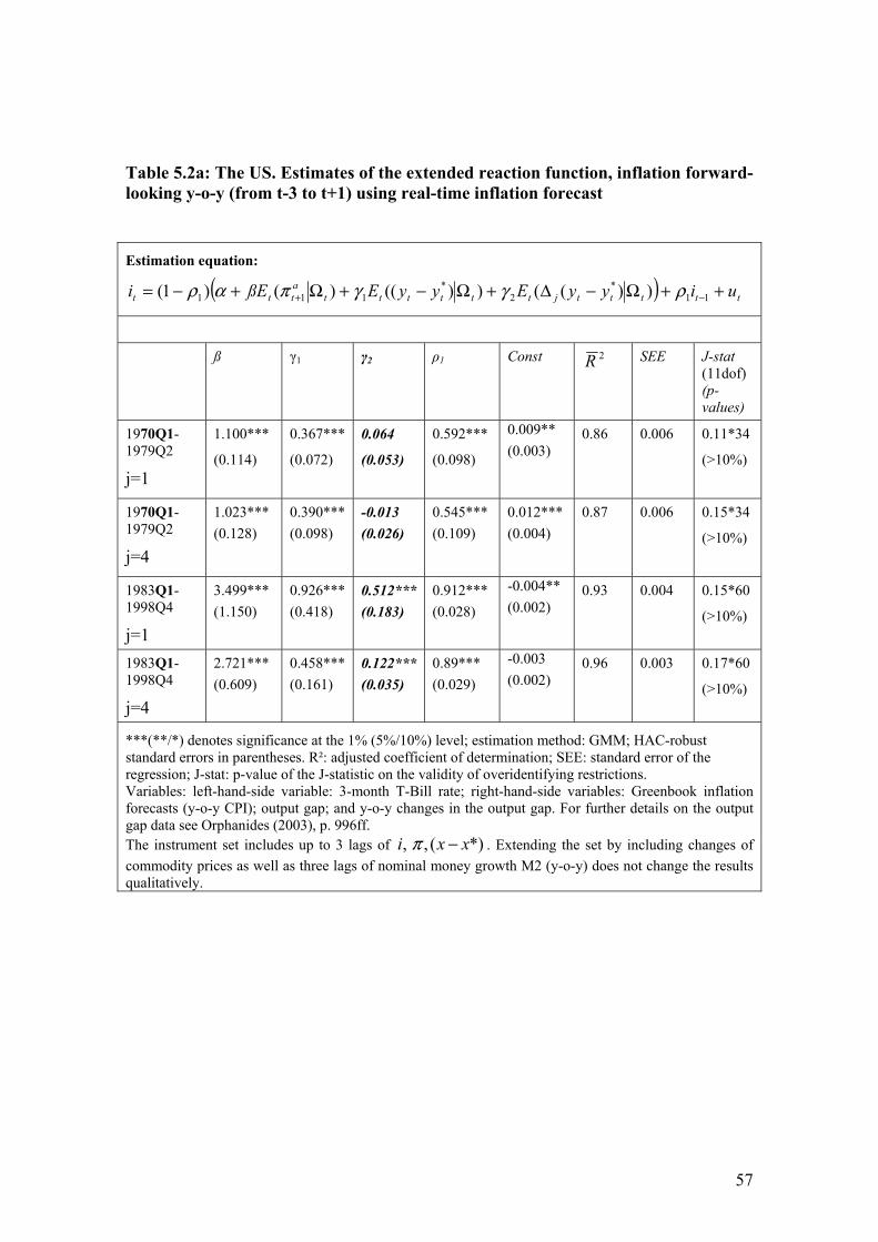
57
Table 5.2a: The US. Estimates of the extended reaction function, inflation forward-looking y-o-y (from t-3 to t+1) using real-time inflation forecast
Estimation equation:
( ) tttttjttttttattt uiyyEyyEßEi ++Ω−Δ+Ω−+Ω+−= −+ 11
*2
*111 ))(())(()()1( ργγπαρ
ß γ1
γ2 ρ1 Const 2R SEE J-stat (11dof) (p-values)
1970Q1-1979Q2
j=1
1.100***
(0.114)
0.367***
(0.072)
0.064
(0.053)
0.592***
(0.098)
0.009** (0.003)
0.86 0.006 0.11*34
(>10%)
1970Q1-1979Q2
j=4
1.023*** (0.128)
0.390*** (0.098)
-0.013 (0.026)
0.545*** (0.109)
0.012*** (0.004)
0.87 0.006 0.15*34
(>10%)
1983Q1-1998Q4
j=1
3.499*** (1.150)
0.926*** (0.418)
0.512*** (0.183)
0.912*** (0.028)
-0.004** (0.002)
0.93 0.004 0.15*60
(>10%)
1983Q1-1998Q4
j=4
2.721*** (0.609)
0.458*** (0.161)
0.122*** (0.035)
0.89*** (0.029)
-0.003 (0.002)
0.96 0.003 0.17*60
(>10%)
***(**/*) denotes significance at the 1% (5%/10%) level; estimation method: GMM; HAC-robust standard errors in parentheses. R²: adjusted coefficient of determination; SEE: standard error of the regression; J-stat: p-value of the J-statistic on the validity of overidentifying restrictions. Variables: left-hand-side variable: 3-month T-Bill rate; right-hand-side variables: Greenbook inflation forecasts (y-o-y CPI); output gap; and y-o-y changes in the output gap. For further details on the output gap data see Orphanides (2003), p. 996ff. The instrument set includes up to 3 lags of , , ( *)i x xπ − . Extending the set by including changes of commodity prices as well as three lags of nominal money growth M2 (y-o-y) does not change the results qualitatively.
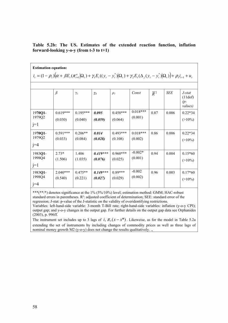
58
Table 5.2b: The US. Estimates of the extended reaction function, inflation forward-looking y-o-y (from t-3 to t+1)
Estimation equation:
( ) tttttjttttttattt uiyyEyyEßEi ++Ω−Δ+Ω−+Ω+−= −+ 11
*2
*111 ))(())(()()1( ργγπαρ
ß γ1
γ2 ρ1 Const 2R SEE J-stat (11dof) (p-values)
1970Q1-1979Q2
j=1
0.619***
(0.030)
0.195***
(0.040)
0.095
(0.059)
0.458***
(0.064)
0.018*** (0.001)
0.87 0.006 0.22*34
(>10%)
1970Q1-1979Q2
j=4
0.591*** (0.033)
0.206** (0.084)
0.014 (0.028)
0.493*** (0.108)
0.018*** (0.002)
0.86 0.006 0.22*34
(>10%)
1983Q1-1998Q4
j=1
2.73* (1.506)
1.406 (1.035)
0.419*** (0.076)
0.960*** (0.025)
-0.002* (0.001)
0.94 0.004 0.15*60
(>10%)
1983Q1-1998Q4
j=4
2.040*** (0.540)
0.475** (0.221)
0.149*** (0.027)
0.89*** (0.029)
-0.002 (0.002)
0.96 0.003 0.17*60
(>10%)
***(**/*) denotes significance at the 1% (5%/10%) level; estimation method: GMM; HAC-robust standard errors in parentheses. R²: adjusted coefficient of determination; SEE: standard error of the regression; J-stat: p-value of the J-statistic on the validity of overidentifying restrictions. Variables: left-hand-side variable: 3-month T-Bill rate; right-hand-side variables: inflation (y-o-y CPI); output gap; and y-o-y changes in the output gap. For further details on the output gap data see Orphanides (2003), p. 996ff. The instrument set includes up to 3 lags of , , ( *)i x xπ − . Likeweise, as for the model in Table 5.2a extending the set of instruments by including changes of commodity prices as well as three lags of nominal money growth M2 (y-o-y) does not change the results qualitatively. .,

59
Table 5.3: The UK. Estimates of the extended reaction function, inflation forward-looking y-o-y (from t-3 to t+1)
Estimation equation:
( ) tttttjttttttattt uiyyEyyEßEi ++Ω−Δ+Ω−+Ω+−= −+ 11
*2
*111 ))(())(()()1( ργγπαρ
ß γ1
γ2 ρ1 Const 2R SEE J-stat (11dof) (p-values)
1970Q1-1979Q2
j=1
-0.10
(0.463)
0.007
(0.34)
0.02
(0.05)
0.869***
(0.10)
0.015*** (0.005)
0.73 0.015 0.24*35
(>10%)
1970Q1-1979Q2
j=4
0.058 (0.33)
-0.02 (0.37)
0.07 (0.083)
0.827*** (0.081)
0.016** (0.006)
0.74 0.014 0.23*35
(>10%)
1983Q1-1996Q1
j=1
1.531*** (0.14)
-0.32 (0.28)
-0.09 (0.095)
0.70*** (0.071)
0.002 (0.002)
0.92 0.0078 0.16*53
(>10%)
1983Q1-1996Q1
j=4
1.526*** (0.156)
-0.20 (0.299)
-0.02 (0.081)
0.72*** (0.069)
0.004 (0.003)
0.92 0.0079 0.16*53
(>10%)
***(**/*) denotes significance at the 1% (5%/10%) level; estimation method: GMM; HAC-robust standard errors in parentheses. R²: adjusted coefficient of determination; SEE: standard error of the regression; J-stat: p-value of the J-statistic on the validity of overidentifying restrictions. Variables: left-hand-side variable: 3-month T-Bill rate; right-hand-side variables: inflation (y-o-y CPI); output gap; and y-o-y changes in the output gap. For further details on the output gap data see Nelson and Nikolov (2003). The instrument set includes up to 3 lags of , , ( *)i x xπ − , and changes of commodity prices as well as three lags of nominal money growth “money + quasi-money” (y-o-y).

60
The following Discussion Papers have been published since 2008:
Series 1: Economic Studies
01 2008 Can capacity constraints explain asymmetries of the business cycle? Malte Knüppel 02 2008 Communication, decision-making and the optimal degree of transparency of monetary policy committees Anke Weber 03 2008 The impact of thin-capitalization rules on Buettner, Overesch multinationals’ financing and investment decisions Schreiber, Wamser 04 2008 Comparing the DSGE model with the factor model: an out-of-sample forecasting experiment Mu-Chun Wang 05 2008 Financial markets and the current account – Sabine Herrmann emerging Europe versus emerging Asia Adalbert Winkler 06 2008 The German sub-national government bond Alexander Schulz market: evolution, yields and liquidity Guntram B. Wolff 07 2008 Integration of financial markets and national Mathias Hoffmann price levels: the role of exchange rate volatility Peter Tillmann 08 2008 Business cycle evidence on firm entry Vivien Lewis 09 2008 Panel estimation of state dependent adjustment when the target is unobserved Ulf von Kalckreuth 10 2008 Nonlinear oil price dynamics – Stefan Reitz a tale of heterogeneous speculators? Ulf Slopek 11 2008 Financing constraints, firm level adjustment of capital and aggregate implications Ulf von Kalckreuth

61
12 2008 Sovereign bond market integration: Alexander Schulz the euro, trading platforms and globalization Guntram B. Wolff 13 2008 Great moderation at the firm level? Claudia M. Buch Unconditional versus conditional output Jörg Döpke volatility Kerstin Stahn 14 2008 How informative are macroeconomic risk forecasts? An examination of the Malte Knüppel Bank of England’s inflation forecasts Guido Schultefrankenfeld 15 2008 Foreign (in)direct investment and corporate taxation Georg Wamser 16 2008 The global dimension of inflation – evidence Sandra Eickmeier from factor-augmented Phillips curves Katharina Moll 17 2008 Global business cycles: M. Ayhan Kose convergence or decoupling? Christopher Otrok, Ewar Prasad 18 2008 Restrictive immigration policy Gabriel Felbermayr in Germany: pains and gains Wido Geis foregone? Wilhelm Kohler 19 2008 International portfolios, capital Nicolas Coeurdacier accumulation and foreign assets Robert Kollmann dynamics Philippe Martin 20 2008 Financial globalization and Michael B. Devereux monetary policy Alan Sutherland 21 2008 Banking globalization, monetary Nicola Cetorelli transmission and the lending channel Linda S. Goldberg 22 2008 Financial exchange rates and international Philip R. Lane currency exposures Jay C. Shambaugh

62
23 2008 Financial integration, specialization F. Fecht, H. P. Grüner and systemic risk P. Hartmann 24 2008 Sectoral differences in wage freezes and Daniel Radowski wage cuts: evidence from a new firm survey Holger Bonin 25 2008 Liquidity and the dynamic pattern of Ansgar Belke price adjustment: a global view Walter Orth, Ralph Setzer 26 2008 Employment protection and Florian Baumann temporary work agencies Mario Mechtel, Nikolai Stähler 27 2008 International financial markets’ influence on the welfare performance of alternative exchange rate regimes Mathias Hoffmann 28 2008 Does regional redistribution spur growth? M. Koetter, M. Wedow 29 2008 International financial competitiveness and incentives to foreign direct investment Axel Jochem 30 2008 The price of liquidity: bank characteristics Falko Fecht and market conditions Kjell G. Nyborg, Jörg Rocholl 01 2009 Spillover effects of minimum wages Christoph Moser in a two-sector search model Nikolai Stähler 02 2009 Who is afraid of political risk? Multinational Iris Kesternich firms and their choice of capital structure Monika Schnitzer 03 2009 Pooling versus model selection for Vladimir Kuzin nowcasting with many predictors: Massimiliano Marcellino an application to German GDP Christian Schumacher

63
04 2009 Fiscal sustainability and Balassone, Cunha, Langenus policy implications for the euro area Manzke, Pavot, Prammer Tommasino 05 2009 Testing for structural breaks Jörg Breitung in dynamic factor models Sandra Eickmeier 06 2009 Price convergence in the EMU? Evidence from micro data Christoph Fischer 07 2009 MIDAS versus mixed-frequency VAR: V. Kuzin, M. Marcellino nowcasting GDP in the euro area C. Schumacher 08 2009 Time-dependent pricing and New Keynesian Phillips curve Fang Yao 09 2009 Knowledge sourcing: Tobias Schmidt legitimacy deficits for MNC subsidiaries? Wolfgang Sofka 10 2009 Factor forecasting using international targeted predictors: the case of German GDP Christian Schumacher 11 2009 Forecasting national activity using lots of international predictors: an application to Sandra Eickmeier New Zealand Tim Ng 12 2009 Opting out of the great inflation: Andreas Beyer, Vitor Gaspar German monetary policy after the Christina Gerberding breakdown of Bretton Woods Otmar Issing

64
Series 2: Banking and Financial Studies 01 2008 Analyzing the interest rate risk of banks using time series of accounting-based data: O. Entrop, C. Memmel evidence from Germany M. Wilkens, A. Zeisler 02 2008 Bank mergers and the dynamics of Ben R. Craig deposit interest rates Valeriya Dinger 03 2008 Monetary policy and bank distress: F. de Graeve an integrated micro-macro approach T. Kick, M. Koetter 04 2008 Estimating asset correlations from stock prices K. Düllmann or default rates – which method is superior? J. Küll, M. Kunisch 05 2008 Rollover risk in commercial paper markets and firms’ debt maturity choice Felix Thierfelder 06 2008 The success of bank mergers revisited – Andreas Behr an assessment based on a matching strategy Frank Heid 07 2008 Which interest rate scenario is the worst one for a bank? Evidence from a tracking bank approach for German savings and cooperative banks Christoph Memmel 08 2008 Market conditions, default risk and Dragon Yongjun Tang credit spreads Hong Yan 09 2008 The pricing of correlated default risk: Nikola Tarashev evidence from the credit derivatives market Haibin Zhu 10 2008 Determinants of European banks’ Christina E. Bannier engagement in loan securitization Dennis N. Hänsel 11 2008 Interaction of market and credit risk: an analysis Klaus Böcker of inter-risk correlation and risk aggregation Martin Hillebrand

65
12 2008 A value at risk analysis of credit default swaps B. Raunig, M. Scheicher 13 2008 Systemic bank risk in Brazil: an assessment of correlated market, credit, sovereign and inter- bank risk in an environment with stochastic Theodore M. Barnhill, Jr. volatilities and correlations Marcos Rietti Souto 14 2008 Regulatory capital for market and credit risk inter- T. Breuer, M. Jandačka action: is current regulation always conservative? K. Rheinberger, M. Summer 15 2008 The implications of latent technology regimes Michael Koetter for competition and efficiency in banking Tigran Poghosyan 16 2008 The impact of downward rating momentum André Güttler on credit portfolio risk Peter Raupach 17 2008 Stress testing of real credit portfolios F. Mager, C. Schmieder 18 2008 Real estate markets and bank distress M. Koetter, T. Poghosyan 19 2008 Stochastic frontier analysis by means of maxi- Andreas Behr mum likelihood and the method of moments Sebastian Tente 20 2008 Sturm und Drang in money market funds: Stehpan Jank when money market funds cease to be narrow Michael Wedow 01 2009 Dominating estimators for the global Gabriel Frahm minimum variance portfolio Christoph Memmel 02 2009 Stress testing German banks in a Klaus Düllmann downturn in the automobile industry Martin Erdelmeier 03 2009 The effects of privatization and consolidation E. Fiorentino on bank productivity: comparative evidence A. De Vincenzo, F. Heid from Italy and Germany A. Karmann, M. Koetter

66
04 2009 Shocks at large banks and banking sector Sven Blank, Claudia M. Buch distress: the Banking Granular Residual Katja Neugebauer 05 2009 Why do savings banks transform sight deposits into illiquid assets less intensively Dorothee Holl than the regulation allows? Andrea Schertler 06 2009 Does banks’ size distort market prices? Manja Völz Evidence for too-big-to-fail in the CDS market Michael Wedow

67
Visiting researcher at the Deutsche Bundesbank
The Deutsche Bundesbank in Frankfurt is looking for a visiting researcher. Among others under certain conditions visiting researchers have access to a wide range of data in the Bundesbank. They include micro data on firms and banks not available in the public. Visitors should prepare a research project during their stay at the Bundesbank. Candidates must hold a PhD and be engaged in the field of either macroeconomics and monetary economics, financial markets or international economics. Proposed research projects should be from these fields. The visiting term will be from 3 to 6 months. Salary is commensurate with experience. Applicants are requested to send a CV, copies of recent papers, letters of reference and a proposal for a research project to: Deutsche Bundesbank Personalabteilung Wilhelm-Epstein-Str. 14 60431 Frankfurt GERMANY