Optimum Setting and Performance Evaluation of the … · Optimum Setting and Performance Evaluation of the Three Mode Controller Using Bio Inspired Soft Computing Algorithms

Optimum Setting and Performance Evaluation of the Three Mode Controller Using Bio Inspired Soft Computing Algorithms

D. M. Mary Synthia Regis Prabha1 G. Glan Devadhas2 S. Pushpa Kumar3 1Associate Professor, EEE Department, Noorul Islam Centre for Higher Education, Kumaracoil, Tamilnadu, India, Pin 629180, email: [email protected], mobile no: +91-9940877270 (Corresponding Author) 2Associate Professor, EIE Department, Noorul Islam Centre for Higher Education, Kumaracoil, India, [email protected] 3Principal,Muthoot Institute of Technology and Science,Varikoli.P.O,Ernakulam, kerala,Puthencruz-682308, [email protected]

Abstract: The best possible and desirable solution of the engineering problems can be found using optimization algorithms. The most widely used dc-dc converters are highly non-linear dynamical systems. Designing a control technique has been a most promising control area. One of the robust non-linear sliding mode controllers has been proved by researchers to be having large signal stability and providing good dynamic response. But the complicated design of the controller as well as the problems encountered during practical implementation gives rise to the necessity to design a controller which gives better performance than the former case and simple in structure and design. The traditional linear three mode PID (Proportional Integral Derivative) controllers which are the most common control algorithm in industries can be properly tuned so that they overcome the performance of the former case. The Bacterial Foraging Optimization Algorithm and Artificial Bee Colony Algorithm have been used for tuning purpose. The best optimization algorithm has been identified and the effectiveness of the PID controller tuned using the best optimization algorithm over the sliding mode controller has been proved. Key words: PID controller, Bacterial Foraging Optimization Algorithm (BFOA), Artificial Bee Colony Algorithm (ABCA), DC-DC Buck Converter, PID Controller, Sliding Mode Controller

1 Introduction

The most commonly encountered mathematical problem in almost all the engineering disciplines is the optimization problem. The best possible and desirable solution of the engineering problems can be found using optimization algorithms. There are a wide range of optimization problems which are yet to be solved which makes this to be an active research area. Naturally, optimization algorithms are seen to be either deterministic or stochastic. Enormous computational efforts are to be put forward to solve optimization problems using the deterministic methods adopted. These methods tend to fail as the problem size increases. The nature inspired optimization algorithms are identified to be computationally efficient alternatives to deterministic methods. The sole inspiration of these algorithms is that derived from nature which reveals their real beauty. These algorithms require little or even no knowledge of the search space which starts from very simple initial conditions and rules for describing and resolving

complex problems. Proper representation of the problem, choosing a correct fitness function for evaluating the quality of problem and creating new solution sets by suitably defining operators are the main steps involved in the design of a bio-inspired algorithm. Switching mode dc-dc converters are widely used today in a variety of applications including power supplies for personal computers, mission critical space applications, laptop computers, dc motor drives, medical electronics as well as high power transmission [1]. The dc-dc converters have high power packing density and high efficiency. So, they are widely used in dc regulation problems. These converters are non-linear dynamical systems. The non-linearities arise primarily due to switching, power switching devices and passive components such as inductors and capacitors. A most promising control area is to design a control technique which is suitable for dc-dc converters to cope up with their intrinsic non-linearities and wide input voltage and load variations ensuring stability in any operating condition while providing fast transient response [2]. PID control which is one of the best known industrial processes is a traditional linear control. It

WSEAS TRANSACTIONS on SYSTEMS and CONTROLD. M. Mary Synthia Regis Prabha,

G. Glan Devadhas, S. Pushpa Kumar

E-ISSN: 2224-2856 163 Volume 11, 2016

mailto:[email protected]

can be easily implemented by engineers using current technologies which make it more popular than other controllers. Linear PID controllers for dc-dc converters are usually designed by classical frequency response techniques applied to the small signal models of converters [3]. Various approaches are available in the literature to determine the PID controller parameters which include Ziegler-Nichols method [4], Cohen-Coon method [5], Internal Model Control based method [6] and Gain-Phase Margin method [7]. In Gain-Phase Margin method the bode-plot of the converter is adjusted in the design to obtain the desired loop gain, cross-over frequency and phase margin. The Sliding Mode Control (SMC) is a type of non-linear control. The SMC has been well known for its large signal stability, robustness and good dynamic response. Moreover the design of an SMC does not require an accurate model of the system. But Sliding Mode Controller even though proved to be more robust in the literatures [8-13] suffers from the drawback of its complicated design procedure. So, it becomes necessary to design a controller which is robust, stable as well as simple in design. So, necessity arises to upgrade the PID controller, which plays an eminent role in industries, to compete with that of the PID based Sliding Mode Controller. It is a well known fact that the PID controller’s performance is decided by the proper selection of the control parameters. So, in order to improve the performance of the controller, and making it superior than that of the sliding mode controller, it becomes necessary to tune the parameters of the PID controller using an algorithm which is efficient in solving hard and complex optimization problems with much less computational time. The various steps involved for finding the optimal controller parameters is called tuning. A best optimization algorithm is one which takes care of the local minima, requires less number of computations and settles in minimum time. The social behaviour of a group of living organisms has attracted the interest of various researchers. In the recent decades, people have developed many population-based optimization algorithms which come under the bio-inspired algorithms for solving complicated engineering problems, imitating the collective foraging behaviour and life system of a group of social insects like ants, bees, termites and wasps or other animal societies. These algorithms are becoming more attractive owing to their immense parallelism, simple computation and its

ability in finding near-optimal solutions to difficult optimization problems. Some of the popular population-based algorithms are the Bacterial Foraging Optimization Algorithm (BFOA) and the Artificial Bee Colony Algorithm (ABCA). The ABCA simulates the behaviour of real bees while finding food sources. BFOA is developed inspired by the social foraging behaviour of Escherichia coli. These optimization algorithms which are finding increasing applications in engineering field are chosen in this paper for optimizing the PID controller parameters because of their capability in handling complex optimization problems, thus rejecting the local minima and finding out the global minima in a wide search space. The basic versions of BFOA and ABCA are utilized in this paper for optimizing the PID controller parameters of a dc-dc Buck converter. In order to make the controllers produce better results, various optimization techniques have been proposed for properly tuning the controller parameters. In 2012, Rajinikanth and Latha [14] proposed an enhanced bacteria foraging optimization algorithm based PID controller tuning for a non-linear chemical process. In 2011, OzdenErcin et.al. [15] studied the performance of the Artificial Bee Colony and the Bees algorithms for proportional-integral-derivative (PID) controller tuning. In 2010, Altinozet. al. [16] applied PSO for achieving improved performance of PID controllers on a Buck converter. In 2010, H. Vahedi [17] compared the BFO algorithm with the Particle Swarm Optimization (PSO) technique for optimizing the parameters of a PID controller. In 2010, Jalilvand [18] illustrated the technique of optimally tuning a PID controlled dc-dc converter using BFOA. In 2010, Abachizadehet. al. [19] studied the performance of Artificial Bee Colony Algorithm optimized PID controller designed for benchmark plants of different orders and time delays and tuned it using Artificial Bee Colony Algorithm. In the literature provided, it can be observed that optimization techniques are applied for tuning of a PID controller designed for various systems. In [18], a dc-dc converter system has been considered for analysis, but it does not provide much information regarding the robustness of the system. This paper gives a detailed procedure for tuning a dc-dc Buck converter using BFOA and ABCA also proves the robustness of the system during line and load disturbances. In this paper, the problem formulation has been explained in section 2. A PID controller has



E-ISSN: 2224-2856 164 Volume 11, 2016

been designed for a dc-dc Buck converter operating in Continuous Conduction Mode which is explained in section 3. Section 4 explains the procedure for optimizing the PID controller parameters using BFOA technique and a detailed performance analysis is made which is also presented in the same section. Section 5 explains the optimization of the controller parameters using ABCA and its performance analysis is also made. Section 6 gives the experimental results. Section 7 presents the results and discussions on the results obtained. It is revealed that the ABCA tuned Buck converter produces better results than that of the BFOA optimized Buck converter. The former case is also compared with Sliding Mode Controlled (SMC) Buck Converter which proves its superiority over the SMC. An experimental study is also made on the ABCA tuned PID controlled Buck Converter which proves its oneness with the simulation results.

2 Problem Formulation 2.1 Control Principle

The PID controller has several parameters that can be adjusted to make the control loop perform better. The controller’s performance deteriorates if the control parameters are not chosen properly. The procedure for finding the controller parameters is called tuning [20]. The PID algorithm can be described as

𝑢𝑢(𝑡𝑡) = 𝐾𝐾𝑒𝑒(𝑡𝑡) +1𝑇𝑇𝑖𝑖𝑒𝑒(𝜏𝜏)𝑡𝑡

0

𝑑𝑑𝜏𝜏 + 𝑇𝑇𝑑𝑑𝑑𝑑𝑒𝑒(𝑡𝑡)𝑑𝑑𝑡𝑡

(1)

𝑢𝑢(𝑡𝑡) = 𝐾𝐾𝑝𝑝𝑒𝑒(𝑡𝑡) + 𝐾𝐾𝑖𝑖 𝑒𝑒(𝜏𝜏)𝑡𝑡

0𝑑𝑑𝜏𝜏 + 𝐾𝐾𝑑𝑑

𝑑𝑑𝑒𝑒(𝑡𝑡)𝑑𝑑𝑡𝑡

(2)

Where u is the control variable and 𝑒𝑒 is the control error. The control variable is thus a sum of three terms: the P term (which is proportional to error), the I-term (which is proportional to the integral of the error), and the D-term (which is proportional to the derivative of the error). While the integral action takes care of the steady state error under steady state condition making it zero, the derivative action improves the closed-loop stability. Proper selection of the controller parameters 𝐾𝐾𝑝𝑝 ,𝐾𝐾𝑖𝑖 and 𝐾𝐾𝑑𝑑 makes the controller perform optimally. This paper is aimed at optimizing the PID controller parameters kp, ki and kd. Some of the figures of merit which are used for evaluating the performance of the control system are Integral of Square Error (ISE), Integral of Absolute Error (IAE) and Integral of Time-Weighted Absolute Error (ITAE). The Integral of the Square of the Error with respect to time (ISE) is often used to evaluate the

response of the control system which is defined as,

𝐼𝐼𝐼𝐼𝐼𝐼 = 𝑉𝑉𝑟𝑟𝑒𝑒𝑟𝑟 − 𝑉𝑉𝑜𝑜𝑢𝑢𝑡𝑡 2(𝑡𝑡) 𝑑𝑑𝑡𝑡

∞

0 (3)

where𝑉𝑉𝑟𝑟𝑒𝑒𝑟𝑟 is the ‘reference voltage’ and 𝑉𝑉𝑜𝑜𝑢𝑢𝑡𝑡 is the ‘actual output voltage’. For a perfectly designed system, with zero offset, this ISE is a single real value. Proper selection of the parameter to produce a minimum ISE value is the main objective in this optimization design problem. Thus the objective of this optimization function can be expressed as

𝜆𝜆 = 𝑉𝑉𝑟𝑟𝑒𝑒𝑟𝑟 − 𝑉𝑉𝑜𝑜𝑢𝑢𝑡𝑡 2(𝑡𝑡) 𝑑𝑑𝑡𝑡 (4)

∞

0

The ISE value will be more for responses having large errors which persist for a long time. It provides a compromise between the reduction of rise time, thus limiting the effect of a large initial error, reduction of the peak overshoot and settling time. The other criteria used in the control process are as follows. Integral of Absolute Value of Error

𝐼𝐼𝐼𝐼𝐼𝐼 = 𝑉𝑉𝑟𝑟𝑒𝑒𝑟𝑟 − 𝑉𝑉𝑜𝑜𝑢𝑢𝑡𝑡 𝑑𝑑𝑡𝑡∞

0 (5)

Integral of Time-Weighted Absolute Error

𝐼𝐼𝑇𝑇𝐼𝐼𝐼𝐼 = 𝑡𝑡𝑉𝑉𝑟𝑟𝑒𝑒𝑟𝑟 − 𝑉𝑉𝑜𝑜𝑢𝑢𝑡𝑡 𝑑𝑑𝑡𝑡∞

0 (6)

ISE strongly suppresses large errors and IAE suppresses small errors more effectively. ITAE works more effectively on errors that persist for a long time. So ISE is used for penalizing the response that has large errors, which is usually the case, in the dynamic portion of the response and ITAE is used for penalizing a response which occurs during the steady state condition. The figure of merit, namely the ISE is often used in optimal control theory because it can be used more easily in mathematical operations than the errors which use the absolute value of error.

2.2 Specification Of Buck Converter The range of input voltage is selected to be from 13V to 30V. The desired output voltage is 12V. The range of load current is selected to be from 0.5A to 4A. The variation of load resistance is from 3Ω to 24Ω. The acceptable output voltage ripple ∆𝑉𝑉𝐶𝐶 is chosen to be 50mV. The peak-to-peak ripple current ∆𝐼𝐼𝐿𝐿of the inductor is normally 25% of the maximum load current which is calculated to be 1A. The time ∆𝑡𝑡 at which the change in the inductor current occurs is given by ∆𝑇𝑇 = 𝐷𝐷

𝑟𝑟= 2.5𝜇𝜇𝜇𝜇.

The peak-to-peak ripple voltage of the capacitor is



E-ISSN: 2224-2856 165 Volume 11, 2016

∆𝑉𝑉𝐶𝐶 = ∆𝐼𝐼𝐿𝐿 𝐼𝐼𝐼𝐼𝐸𝐸 + ∆𝑇𝑇𝐶𝐶. The ESR value of an

electrolytic capacitor used is chosen as 0.03Ω as specified by the manufacturer and the ESR value of the inductor is chosen as 0.12Ω. Hence, the capacitance value is calculated to be 125μF. The capacitor value is selected as 150μF which is normally chosen to be greater than the calculated value. The critical value for inductance is calculated using the formula 𝐿𝐿𝑐𝑐𝑟𝑟𝑖𝑖𝑡𝑡 = (1−𝐷𝐷)𝐸𝐸𝑚𝑚𝑚𝑚𝑚𝑚

2𝑟𝑟= 30𝜇𝜇𝜇𝜇 (7)

3. Design of a PID Controller in Continuous Conduction Mode The open loop transfer function G(s) H(s) is given as, 𝑉𝑉0(𝜇𝜇)𝑑𝑑(𝜇𝜇)

=

𝑉𝑉𝑜𝑜𝐷𝐷 1+𝜇𝜇𝐸𝐸𝐶𝐶𝐶𝐶

1+𝜇𝜇𝐸𝐸𝐶𝐶𝐶𝐶+ 𝐸𝐸𝐿𝐿𝐸𝐸𝑜𝑜𝐸𝐸𝐿𝐿+𝐸𝐸𝑜𝑜

𝐶𝐶+ 𝐿𝐿𝐸𝐸𝐿𝐿+𝐸𝐸𝑜𝑜

+𝜇𝜇2𝐿𝐿𝐶𝐶𝐸𝐸𝑜𝑜+𝐸𝐸𝐶𝐶𝐸𝐸𝑜𝑜+𝐸𝐸𝐿𝐿

(8)

The prototype Buck converter is made to operate with the given nominal operating point. Input Voltage, Vin =24V, Desired Output Voltage, Vod = 12 V, Duty ratio D = 0.5. The switch is made to operate at a frequency of 200 kHz. The converter is designed for a variation in load resistance ranging from 3Ω to 24Ω. For a load resistance of Ro=6 Ω, Filter Inductance, L =35 μH, which is greater than 𝐿𝐿𝑐𝑐𝑟𝑟𝑖𝑖𝑡𝑡 , the value required to make it to operate in CCM, Filter Capacitance, C =150 μF, ESR of Inductor, RL=0.12 Ω and ESR of Capacitor, RC=0.03 Ω, the transfer function becomes,

𝑉𝑉𝑜𝑜(𝜇𝜇)𝑑𝑑(𝜇𝜇)

= 24+10.8𝑒𝑒−4𝜇𝜇1+5.817𝑒𝑒−4𝜇𝜇+4.243𝑒𝑒−9𝜇𝜇2 (9)

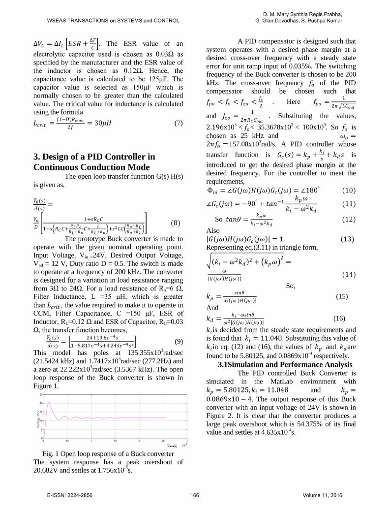
This model has poles at 135.355x103rad/sec (21.5424 kHz) and 1.7417x103rad/sec (277.2Hz) and a zero at 22.222x103rad/sec (3.5367 kHz). The open loop response of the Buck converter is shown in Figure 1.

Fig. 1 Open loop response of a Buck converter

The system response has a peak overshoot of 20.682V and settles at 1.756x10-3s.

A PID compensator is designed such that system operates with a desired phase margin at a desired cross-over frequency with a steady state error for unit ramp input of 0.035%. The switching frequency of the Buck converter is chosen to be 200 kHz. The cross-over frequency 𝑟𝑟𝑜𝑜 of the PID compensator should be chosen such that 𝑟𝑟𝑝𝑝𝑜𝑜 < 𝑟𝑟𝑜𝑜 < 𝑟𝑟𝑧𝑧𝑜𝑜 < 𝑟𝑟𝜇𝜇

2. Here 𝑟𝑟𝑝𝑝𝑜𝑜 = 1

2𝜋𝜋𝐿𝐿𝐶𝐶𝑜𝑜𝑢𝑢𝑡𝑡

and 𝑟𝑟𝑧𝑧𝑜𝑜 = 12𝜋𝜋𝐸𝐸𝐶𝐶𝐶𝐶𝑜𝑜𝑢𝑢𝑡𝑡

. Substituting the values, 2.196x103 < 𝑟𝑟𝑜𝑜< 35.3678x103 < 100x103. So 𝑟𝑟𝑜𝑜 is chosen as 25 kHz and 𝜔𝜔𝑜𝑜 =2𝜋𝜋𝑟𝑟𝑜𝑜 =157.08x103rad/s. A PID controller whose transfer function is 𝐺𝐺𝑐𝑐(𝜇𝜇) = 𝑘𝑘𝑝𝑝 + 𝑘𝑘𝑖𝑖

𝜇𝜇+ 𝑘𝑘𝑑𝑑𝜇𝜇 is

introduced to get the desired phase margin at the desired frequency. For the controller to meet the requirements, Ф𝑚𝑚 = ∠𝐺𝐺(𝑗𝑗𝜔𝜔)𝜇𝜇(𝑗𝑗𝜔𝜔)𝐺𝐺𝑐𝑐(𝑗𝑗𝜔𝜔) = ∠180° (10)

∠𝐺𝐺𝑐𝑐(𝑗𝑗𝜔𝜔) = −90° + 𝑡𝑡𝑚𝑚𝑡𝑡−1 𝑘𝑘𝑝𝑝𝜔𝜔𝑘𝑘𝑖𝑖 − 𝜔𝜔2𝑘𝑘𝑑𝑑

(11)

So 𝑡𝑡𝑚𝑚𝑡𝑡𝑡𝑡 = 𝑘𝑘𝑝𝑝𝜔𝜔𝑘𝑘𝑖𝑖−𝜔𝜔2𝑘𝑘𝑑𝑑

(12) Also |𝐺𝐺(𝑗𝑗𝜔𝜔)𝜇𝜇(𝑗𝑗𝜔𝜔)𝐺𝐺𝑐𝑐(𝑗𝑗𝜔𝜔)| = 1 (13) Representing eq.(3.11) in triangle form,

(𝑘𝑘𝑖𝑖 − 𝜔𝜔2𝑘𝑘𝑑𝑑)2 + 𝑘𝑘𝑝𝑝𝜔𝜔2 =

𝜔𝜔|𝐺𝐺(𝑗𝑗𝜔𝜔 )𝜇𝜇(𝑗𝑗𝜔𝜔 )| (14) So, 𝑘𝑘𝑝𝑝 = 𝜇𝜇𝑖𝑖𝑡𝑡𝑡𝑡

|𝐺𝐺(𝑗𝑗𝜔𝜔 )𝜇𝜇(𝑗𝑗𝜔𝜔 )| (15) And 𝑘𝑘𝑑𝑑 = 𝑘𝑘𝑖𝑖−𝜔𝜔𝜇𝜇𝑖𝑖𝑡𝑡𝑡𝑡

𝜔𝜔2|𝐺𝐺(𝑗𝑗𝜔𝜔 )𝜇𝜇(𝑗𝑗𝜔𝜔 )| (16) 𝑘𝑘𝑖𝑖 is decided from the steady state requirements and is found that 𝑘𝑘𝑖𝑖 = 11.048. Substituting this value of 𝑘𝑘𝑖𝑖 in eq. (12) and (16), the values of 𝑘𝑘𝑝𝑝 and 𝑘𝑘𝑑𝑑are found to be 5.80125, and 0.0869x10-4 respectively.

3.1Simulation and Performance Analysis The PID controlled Buck Converter is simulated in the MatLab environment with 𝑘𝑘𝑝𝑝 = 5.80125,𝑘𝑘𝑖𝑖 = 11.048 and 𝑘𝑘𝑝𝑝 =0.0869x10− 4. The output response of this Buck converter with an input voltage of 24V is shown in Figure 2. It is clear that the converter produces a large peak overshoot which is 54.375% of its final value and settles at 4.635x10-4s.



E-ISSN: 2224-2856 166 Volume 11, 2016

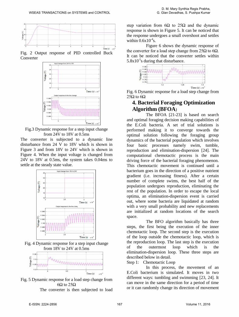
Fig. 2 Output response of PID controlled Buck Converter

Fig.3 Dynamic response for a step input change

from 24V to 18V at 0.5ms The converter is subjected to a dynamic line disturbance from 24 V to 18V which is shown in Figure 3 and from 18V to 24V which is shown in Figure 4. When the input voltage is changed from 24V to 18V at 0.5ms, the system takes 0.04ms to settle at the steady state value.

Fig. 4 Dynamic response for a step input change

from 18V to 24V at 0.5ms

Fig. 5 Dynamic response for a load step change from

6Ω to 25Ω The converter is then subjected to load

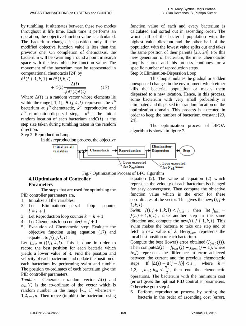
step variation from 6Ω to 25Ω and the dynamic response is shown in Figure 5. It can be noticed that the response undergoes a small overshoot and settles within 0.6x10-4s. Figure 6 shows the dynamic response of the converter for a load step change from 25Ω to 6Ω. It can be noticed that the converter settles within 5.8x10-5s during that disturbance.

Fig. 6 Dynamic response for a load step change from 25Ω to 6Ω

4. Bacterial Foraging Optimization Algorithm (BFOA)

The BFOA [21-23] is based on search and optimal foraging decision making capabilities of the E.Coli bacteria. A set of trial solutions is performed making it to converge towards the optimal solution following the foraging group dynamics of the bacterial population which involves four basic processes namely swim, tumble, reproduction and elimination-dispersion [24]. The computational chemotactic process is the main driving force of the bacterial foraging phenomenon. This chemotactic movement is continued until a bacterium goes in the direction of a positive nutrient gradient (i.e. increasing fitness). After a certain number of complete swims, the best half of the population undergoes reproduction, eliminating the rest of the population. In order to escape the local optima, an elimination-dispersion event is carried out, where some bacteria are liquidated at random with a very small probability and new replacements are initialized at random locations of the search space. The BFO algorithm basically has three steps, the first being the execution of the inner chemotactic loop. The second step is the execution of the loop outside the chemotactic loop, which is the reproduction loop. The last step is the execution of the outermost loop which is the elimination-dispersion loop. These three steps are described below in detail. Step 1: Chemotactic Loop In this process, the movement of an E.Coli bacterium is simulated. It moves in two different ways: tumbling and swimming [23, 24]. It can move in the same direction for a period of time or it can randomly change its direction of movement



E-ISSN: 2224-2856 167 Volume 11, 2016

by tumbling. It alternates between these two modes throughout it life time. Each time it performs an operation, the objective function value is calculated. The bacterium changes its position only if the modified objective function value is less than the previous one. On completion of chemotaxis, the bacterium will be swarming around a point in search space with the least objective function value. The movement of the bacterium may be represented in computational chemotaxis [24] by 𝑡𝑡𝑖𝑖(𝑗𝑗 + 1,𝑘𝑘, 1) = 𝑡𝑡𝑖𝑖(𝑗𝑗,𝑘𝑘, 𝑙𝑙)

+ 𝐶𝐶(𝑖𝑖)∆(𝑖𝑖)

∆𝜏𝜏(𝑖𝑖)∆(𝑖𝑖) (17)

Where ∆(𝑖𝑖) is a random vector whose elements lie within the range [-1, 1], 𝑡𝑡𝑖𝑖(𝑗𝑗,𝑘𝑘, 𝑙𝑙) represents the 𝑖𝑖th

bacterium at 𝑗𝑗th chemotactic, 𝑘𝑘 th reproductive and 𝑙𝑙 th elimination-dispersal step, 𝑡𝑡𝑖𝑖 is the initial random location of each bacterium and𝐶𝐶(𝑖𝑖) is the step size taken during tumbling taken in the random direction. Step 2: Reproduction Loop In this reproduction process, the objective

function value of each and every bacterium is calculated and sorted out in ascending order. The worst half of the bacterial population with the highest value dies out and the other half of the population with the lowest value splits out and takes the same position of their parents [23, 24]. For this new generation of bacterium, the inner chemotactic loop is started and this process continues for a specific number of reproduction steps. Step 3: Elimination-Dispersion Loop This loop simulates the gradual or sudden unexpected changes in the environment which either kills the bacterial population or makes them dispersed to a new location. Hence, in this process, some bacterium with very small probability is eliminated and dispersed to a random location on the optimization domain. This process is executed in order to keep the number of bacterium constant [23, 24]. The optimization process of BFOA algorithm is shown in figure 7.

Fig.7 Optimization Process of BFO algorithm

4.1Optimization of Controller Parameters

The steps that are used for optimizing the PID controller parameters are, 1. Initialize all the variables. 2. Let Elimination/dispersal loop counter

𝑙𝑙 = 𝑙𝑙 + 1 3. Let Reproduction loop counter 𝑘𝑘 = 𝑘𝑘 + 1 4. Let Chemotaxis loop counter𝑗𝑗 = 𝑗𝑗 + 1 5. Execution of Chemotactic step: Evaluate the

objective function using equation (17) and equate it to 𝐽𝐽(𝑖𝑖, 𝑗𝑗,𝑘𝑘, 𝑙𝑙).

Let 𝐽𝐽𝑙𝑙𝑚𝑚𝜇𝜇𝑡𝑡 = 𝐽𝐽(𝑖𝑖, 𝑗𝑗,𝑘𝑘, 𝑙𝑙). This is done in order to record the best position for each bacteria which yields a lower value of 𝜆𝜆. Find the position and velocity of each bacterium and update the position of each bacterium by performing swim and tumble. The position co-ordinates of each bacterium give the PID controller parameters. Tumble: Generate a random vector 𝛥𝛥(𝑖𝑖) and 𝛥𝛥𝑚𝑚 (𝑖𝑖) is the co-ordinate of the vector which is random number in the range [-1, 1] where 𝑚𝑚 =1,2, … ,𝑝𝑝. Then move (tumble) the bacterium using

equation (2). The value of equation (2) which represents the velocity of each bacterium is changed for easy convergence. Then compute the objective function value which is the error for these co-ordinates of the vector. This gives the new𝐽𝐽(𝑖𝑖, 𝑗𝑗 +1,𝑘𝑘, 𝑙𝑙). Swim: 𝐽𝐽(𝑖𝑖, 𝑗𝑗 + 1,𝑘𝑘, 𝑙𝑙) < 𝐽𝐽𝑙𝑙𝑚𝑚𝜇𝜇𝑡𝑡 , then let 𝐽𝐽𝑙𝑙𝑚𝑚𝜇𝜇𝑡𝑡 =𝐽𝐽(𝑖𝑖, 𝑗𝑗 + 1,𝑘𝑘, 𝑙𝑙) , take another step in the same direction and compute the new𝐽𝐽(𝑖𝑖, 𝑗𝑗 + 1,𝑘𝑘, 𝑙𝑙). This swim makes the bacteria to take one step and to fetch a new value of 𝜆𝜆. Here𝐽𝐽𝑙𝑙𝑚𝑚𝜇𝜇𝑡𝑡 represents the local best position of each bacterium. Compute the best (lower) error obtained (𝐽𝐽𝑏𝑏𝑒𝑒𝜇𝜇𝑡𝑡 (𝑗𝑗)). Then compute∆(𝑗𝑗) = 𝐽𝐽𝑏𝑏𝑒𝑒𝜇𝜇𝑡𝑡 (𝑗𝑗) − 𝐽𝐽𝑏𝑏𝑒𝑒𝜇𝜇𝑡𝑡 (𝑗𝑗 − 1), where ∆(𝑗𝑗) represents the difference in error achieved between the current and the previous chemotactic steps. If |∆(𝑗𝑗)− ∆(𝑗𝑗 − ℎ)| < 𝜀𝜀 , where ℎ =1,2, … ,ℎ𝑚𝑚 ; ℎ𝑚𝑚 < 𝑁𝑁𝑐𝑐𝜇𝜇

2, then end the chemotactic

operations. The bacterium with the minimum cost (error) gives the optimal PID controller parameters. Otherwise goto step 4. 6. Perform reproduction process by sorting the

bacteria in the order of ascending cost (error),



E-ISSN: 2224-2856 168 Volume 11, 2016

killing half of the population with highest cost and splitting up the other half population. If 𝑘𝑘 < 𝑁𝑁𝑟𝑟𝑒𝑒𝑝𝑝 , then goto step 3.

7. Perform Elimination/Dispersal process by randomly eliminating the bacteria with probability 𝑃𝑃𝑒𝑒𝑑𝑑 and dispersing each bacterium in a new location for maintaining the number of bacteria constant. This process helps the dispersed bacterium to take entirely new parameter values. If 𝑙𝑙 < 𝑁𝑁𝑒𝑒𝑑𝑑 , then goto step 2.

4.2 Simulation And Performance Analysis The PID controller parameters are being optimized using the BFOA algorithm. The variables used in BFOA are assigned the values given below. It is then simulated in MatLab environment.

i. Dimension of search space D=3 ii. The number of bacteria NB =10

iii. Number of chemotactic steps Ncs =10 iv. Limits the length of a swim Nsl =4 v. The number of reproduction steps Nrep=4

vi. The number of elimination-dispersal events Nede=1

vii. The number of bacteria reproductions (splits) per generation Sr=s/2

viii. The probability that each bacteria will be eliminated/dispersed Ped=0.25

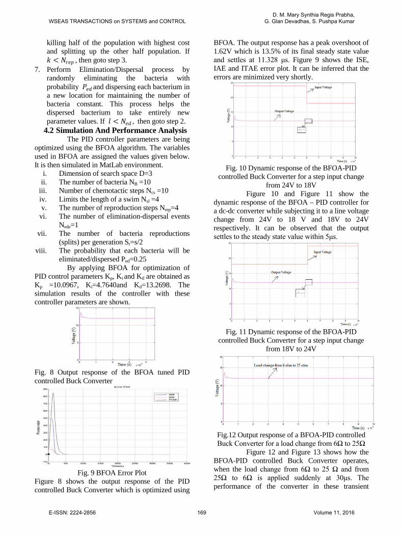
By applying BFOA for optimization of PID control parameters Kp, Ki and Kd are obtained as Kp =10.0967, Ki=4.7640and Kd=13.2698. The simulation results of the controller with these controller parameters are shown.

Fig. 8 Output response of the BFOA tuned PID controlled Buck Converter

Fig. 9 BFOA Error Plot Figure 8 shows the output response of the PID controlled Buck Converter which is optimized using

BFOA. The output response has a peak overshoot of 1.62V which is 13.5% of its final steady state value and settles at 11.328 μs. Figure 9 shows the ISE, IAE and ITAE error plot. It can be inferred that the errors are minimized very shortly.

Fig. 10 Dynamic response of the BFOA-PID

controlled Buck Converter for a step input change from 24V to 18V

Figure 10 and Figure 11 show the dynamic response of the BFOA – PID controller for a dc-dc converter while subjecting it to a line voltage change from 24V to 18 V and 18V to 24V respectively. It can be observed that the output settles to the steady state value within 5μs.

Fig. 11 Dynamic response of the BFOA-PID

controlled Buck Converter for a step input change from 18V to 24V

Fig.12 Output response of a BFOA-PID controlled Buck Converter for a load change from 6Ω to 25Ω

Figure 12 and Figure 13 shows how the BFOA-PID controlled Buck Converter operates, when the load change from 6Ω to 25 Ω and from 25Ω to 6Ω is applied suddenly at 30μs. The performance of the converter in these transient



E-ISSN: 2224-2856 169 Volume 11, 2016

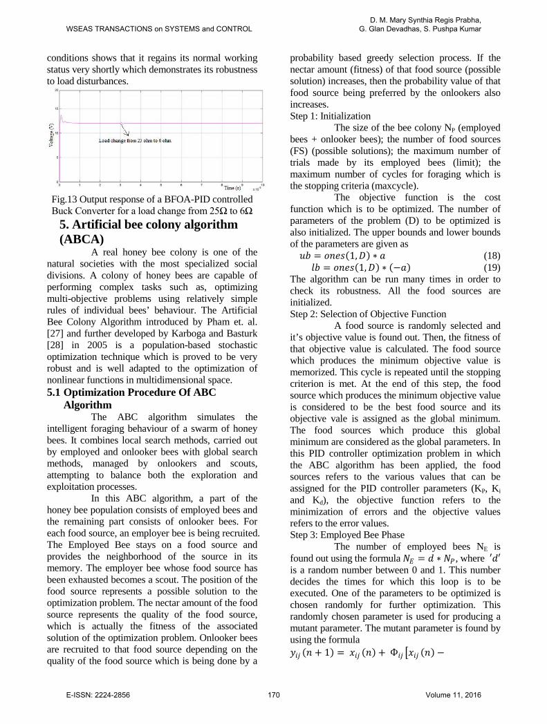
conditions shows that it regains its normal working status very shortly which demonstrates its robustness to load disturbances.

Fig.13 Output response of a BFOA-PID controlled Buck Converter for a load change from 25Ω to 6Ω

5. Artificial bee colony algorithm (ABCA)

A real honey bee colony is one of the natural societies with the most specialized social divisions. A colony of honey bees are capable of performing complex tasks such as, optimizing multi-objective problems using relatively simple rules of individual bees’ behaviour. The Artificial Bee Colony Algorithm introduced by Pham et. al. [27] and further developed by Karboga and Basturk [28] in 2005 is a population-based stochastic optimization technique which is proved to be very robust and is well adapted to the optimization of nonlinear functions in multidimensional space. 5.1 Optimization Procedure Of ABC

Algorithm The ABC algorithm simulates the intelligent foraging behaviour of a swarm of honey bees. It combines local search methods, carried out by employed and onlooker bees with global search methods, managed by onlookers and scouts, attempting to balance both the exploration and exploitation processes. In this ABC algorithm, a part of the honey bee population consists of employed bees and the remaining part consists of onlooker bees. For each food source, an employer bee is being recruited. The Employed Bee stays on a food source and provides the neighborhood of the source in its memory. The employer bee whose food source has been exhausted becomes a scout. The position of the food source represents a possible solution to the optimization problem. The nectar amount of the food source represents the quality of the food source, which is actually the fitness of the associated solution of the optimization problem. Onlooker bees are recruited to that food source depending on the quality of the food source which is being done by a

probability based greedy selection process. If the nectar amount (fitness) of that food source (possible solution) increases, then the probability value of that food source being preferred by the onlookers also increases. Step 1: Initialization The size of the bee colony NP (employed bees + onlooker bees); the number of food sources (FS) (possible solutions); the maximum number of trials made by its employed bees (limit); the maximum number of cycles for foraging which is the stopping criteria (maxcycle). The objective function is the cost function which is to be optimized. The number of parameters of the problem (D) to be optimized is also initialized. The upper bounds and lower bounds of the parameters are given as 𝑢𝑢𝑏𝑏 = 𝑜𝑜𝑡𝑡𝑒𝑒𝜇𝜇(1,𝐷𝐷) ∗ 𝑚𝑚 (18) 𝑙𝑙𝑏𝑏 = 𝑜𝑜𝑡𝑡𝑒𝑒𝜇𝜇(1,𝐷𝐷) ∗ (−𝑚𝑚) (19)

The algorithm can be run many times in order to check its robustness. All the food sources are initialized. Step 2: Selection of Objective Function A food source is randomly selected and it’s objective value is found out. Then, the fitness of that objective value is calculated. The food source which produces the minimum objective value is memorized. This cycle is repeated until the stopping criterion is met. At the end of this step, the food source which produces the minimum objective value is considered to be the best food source and its objective vale is assigned as the global minimum. The food sources which produce this global minimum are considered as the global parameters. In this PID controller optimization problem in which the ABC algorithm has been applied, the food sources refers to the various values that can be assigned for the PID controller parameters (KP, Ki and Kd), the objective function refers to the minimization of errors and the objective values refers to the error values. Step 3: Employed Bee Phase The number of employed bees NE is found out using the formula 𝑁𝑁𝐼𝐼 = 𝑑𝑑 ∗ 𝑁𝑁𝑃𝑃 , where ′𝑑𝑑′ is a random number between 0 and 1. This number decides the times for which this loop is to be executed. One of the parameters to be optimized is chosen randomly for further optimization. This randomly chosen parameter is used for producing a mutant parameter. The mutant parameter is found by using the formula 𝑦𝑦𝑖𝑖𝑗𝑗 (𝑡𝑡 + 1) = 𝑚𝑚𝑖𝑖𝑗𝑗 (𝑡𝑡) + Ф𝑖𝑖𝑗𝑗 𝑚𝑚𝑖𝑖𝑗𝑗 (𝑡𝑡)−



E-ISSN: 2224-2856 170 Volume 11, 2016

𝑚𝑚𝑘𝑘𝑗𝑗 (𝑡𝑡) (20) Where 𝑖𝑖 = 1,2, … ,𝐹𝐹𝐼𝐼,𝑘𝑘 = 1,2, … ,𝐹𝐹𝐼𝐼 and𝑗𝑗 = 1,2, … ,𝐷𝐷, 𝑦𝑦𝑖𝑖𝑗𝑗 (𝑡𝑡 + 1)represents the new mutant parameter value that the employed bee finds at the search step (n +1), 𝑚𝑚𝑖𝑖𝑗𝑗 (𝑡𝑡) represents the optimum value of the parameter that the employed bee in the same food source finds at the search step(𝑡𝑡), 𝑚𝑚𝑘𝑘𝑗𝑗 (𝑡𝑡) is the value of the parameter which is selected randomly, ‘D’ is the number of parameters to be optimized and ′𝐹𝐹𝐼𝐼′ is the number of food sources. Thus, the employed bees in every food source exploit the neighbourhood of their own food sources. If the newly generated parameter value is out of boundaries, it is shifted onto the boundaries. The fitness value of that new mutant parameter is then calculated. A greedy selection is applied between the current randomly chosen parameter and it’s new mutant parameter. If the fitness value of the new mutant parameter (fitnesssol) is better than that of current parameter (fitness(i)), then replace the current randomly chosen parameter value with that of the new parameter value. If the fitness value has not improved, then repeat the same steps and go for a next trial. This trial is made for NE times. Step 4: Calculate Probabilities A food source is chosen with a probability which is proportional to its quality. Probability values can be calculated by using the fitness values and normalizing it by dividing with the maximum fitness value.

𝑃𝑃(𝑖𝑖) = 𝑏𝑏∗𝑟𝑟𝑖𝑖𝑡𝑡𝑡𝑡𝑒𝑒𝜇𝜇𝜇𝜇 (𝑖𝑖)𝑚𝑚𝑚𝑚𝑚𝑚 (𝑟𝑟𝑖𝑖𝑡𝑡𝑡𝑡𝑒𝑒𝜇𝜇𝜇𝜇 ) + 𝑐𝑐 (21)

Step 4: Onlooker Bee Phase Onlookers are assigned to every food source in order to exploit the neighbourhood of the food sources according to the probability calculated in equation (5.4). Hence, the number of onlookers(𝑁𝑁𝑂𝑂𝑁𝑁) in every food source is expressed as 𝑁𝑁𝑂𝑂𝑁𝑁 = 𝑁𝑁𝑃𝑃 ∗ 𝑒𝑒 (22) Where 𝑒𝑒 = 1 − 𝑑𝑑 , which is a random number varying between 0 and 1. These onlooker bees also exploit the neighbourhood of their own food source as given by equation (20). They follow the same greedy selection procedure as that followed by the employed bees and the trial is made for 𝑁𝑁𝑂𝑂𝑁𝑁 times with the condition that the randomly chosen procedure is less the probability 𝑃𝑃(𝑖𝑖), 𝑖𝑖. 𝑒𝑒. , 𝑟𝑟𝑚𝑚𝑡𝑡𝑑𝑑 < 𝑝𝑝𝑟𝑟𝑜𝑜𝑏𝑏(𝑖𝑖). At the end of this phase, the best parameter value which produces the minimum objective value is memorized. Once again, this objective value is compared with the global minimum obtained step 1, to check if this

memorized objective value is less than that of the global minimum, i.e., if 𝑂𝑂𝑏𝑏𝑗𝑗𝑉𝑉𝑚𝑚𝑙𝑙(𝑖𝑖) < 𝐺𝐺𝑙𝑙𝑜𝑜𝑏𝑏𝑚𝑚𝑙𝑙𝐺𝐺𝑖𝑖𝑡𝑡, then 𝐺𝐺𝑙𝑙𝑜𝑜𝑏𝑏𝑚𝑚𝑙𝑙𝐺𝐺𝑖𝑖𝑡𝑡 = 𝑂𝑂𝑏𝑏𝑗𝑗𝑉𝑉𝑚𝑚𝑙𝑙(𝑖𝑖) . The parameters yielding this 𝐺𝐺𝑙𝑙𝑜𝑜𝑏𝑏𝑚𝑚𝑙𝑙𝐺𝐺𝑖𝑖𝑡𝑡 are considered as the Global Parameters (𝐺𝐺𝑙𝑙𝑜𝑜𝑏𝑏𝑚𝑚𝑙𝑙𝑃𝑃𝑚𝑚𝑟𝑟𝑚𝑚𝑚𝑚𝜇𝜇). Step 5: Scout Bee Phase For some food sources, the employed bees and the onlooker bees may not be able to find out the optimum position, even though the trial counter exceeds the ‘limit’ value. In such case, those bees become scout bees and enter into the Scout Bee Phase. In this phase, one scout is allowed to occur in one cycle. The Scout bee carries out an exploration step to discover new parameter values with a new optimized objective value. This exploration is carried out based on the equation (23).

𝑦𝑦𝑖𝑖𝑗𝑗 = 𝑟𝑟𝑚𝑚𝑡𝑡𝑑𝑑 (1,𝐷𝐷) ∗ (𝑢𝑢𝑏𝑏 − 𝑙𝑙𝑏𝑏) + 𝑙𝑙𝑏𝑏 (23)

Where 𝑢𝑢𝑏𝑏 = upper bound of the parameters, 𝑙𝑙𝑏𝑏 = lower bound of the parameters, 𝐷𝐷 = number of parameters in the search space, 𝑦𝑦𝑖𝑖𝑗𝑗 = new value of the parameter. The steps (2) to (6) are repeated until the stopping criterion is met. 5.2 Simulation And Performance Analysis The ABC algorithm is used for optimizing the controller parameters of the PID controller of a Buck Converter. The values assigned for the control parameters of the ABC algorithm are:

• Colony Size NP = 20 • Number of food sources FS = 10 • Number of Employer Bees NE =10 • Number on onlooker bees = NON = 10 • Limit = 100 • Maximum Cycle = 25 • Number of parameters to be optimized = D

= 3 By applying ABCA, the PID control parameters are optimized and the control parameters Kp, Ki and Kd are obtained as Kp=79.2547, Ki=1.7399 and Kd=35.8917. The MatLab simulation results of the controller with these controller parameters are shown.

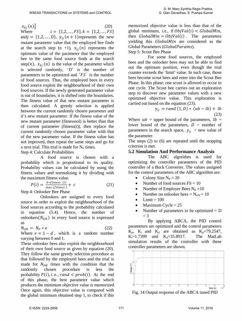
Fig. 14 Output response of the ABCA tuned PID



E-ISSN: 2224-2856 171 Volume 11, 2016

controlled Buck Converter The output voltage settles in 1.9x10 -6s with negligible overshoot. This is clear from Figure 14.

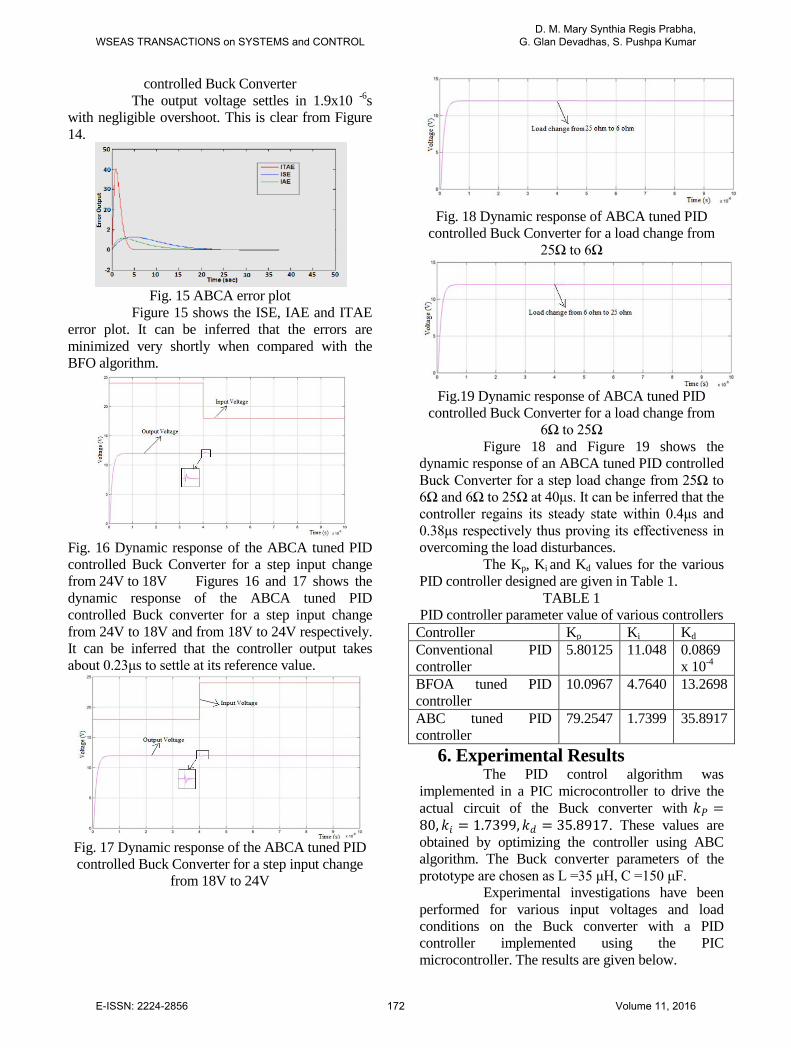
Fig. 15 ABCA error plot

Figure 15 shows the ISE, IAE and ITAE error plot. It can be inferred that the errors are minimized very shortly when compared with the BFO algorithm.

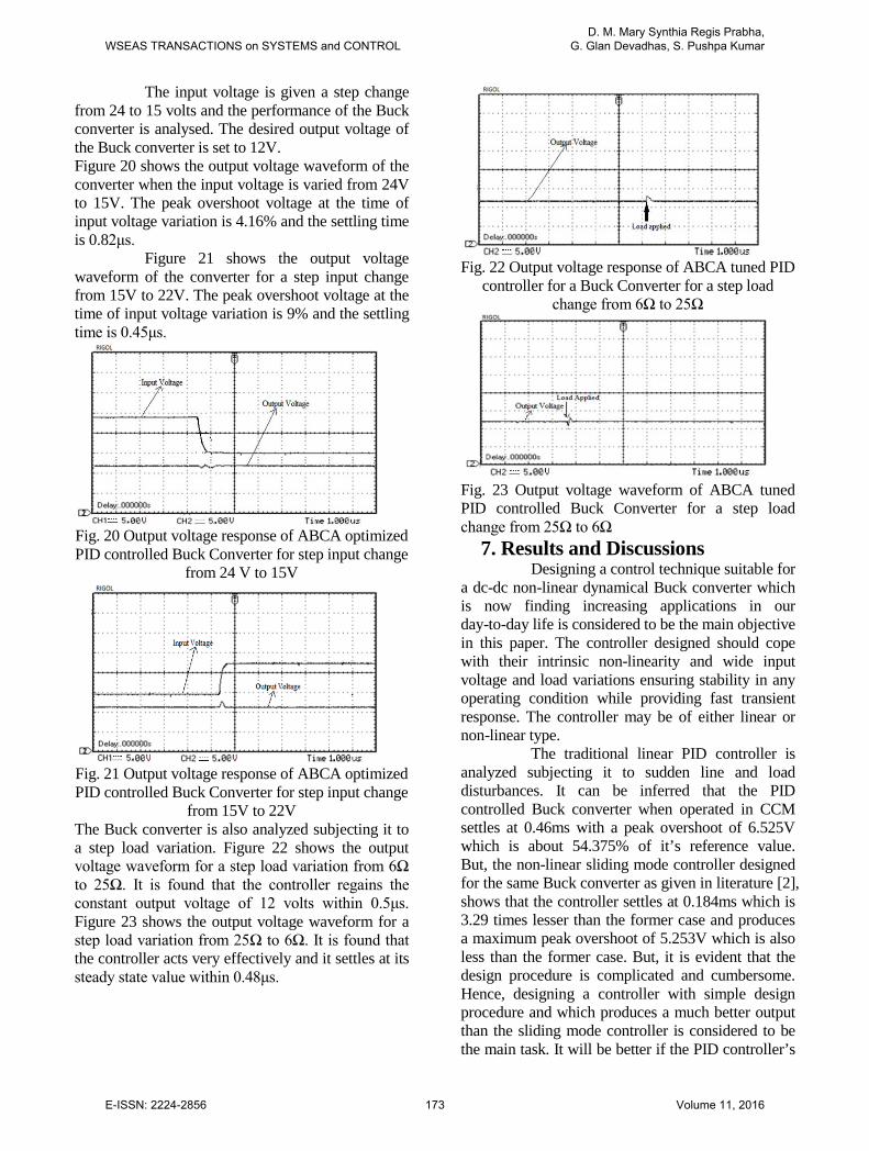
Fig. 16 Dynamic response of the ABCA tuned PID controlled Buck Converter for a step input change from 24V to 18V Figures 16 and 17 shows the dynamic response of the ABCA tuned PID controlled Buck converter for a step input change from 24V to 18V and from 18V to 24V respectively. It can be inferred that the controller output takes about 0.23μs to settle at its reference value.

Fig. 17 Dynamic response of the ABCA tuned PID controlled Buck Converter for a step input change

from 18V to 24V

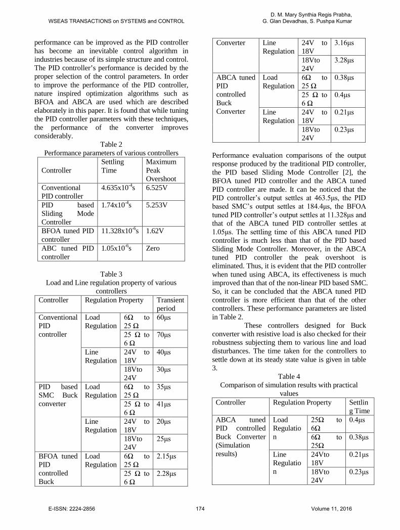
Fig. 18 Dynamic response of ABCA tuned PID

controlled Buck Converter for a load change from 25Ω to 6Ω

Fig.19 Dynamic response of ABCA tuned PID controlled Buck Converter for a load change from

6Ω to 25Ω Figure 18 and Figure 19 shows the dynamic response of an ABCA tuned PID controlled Buck Converter for a step load change from 25Ω to 6Ω and 6Ω to 25Ω at 40μs. It can be inferred that the controller regains its steady state within 0.4μs and 0.38μs respectively thus proving its effectiveness in overcoming the load disturbances. The Kp, Ki and Kd values for the various PID controller designed are given in Table 1.

TABLE 1 PID controller parameter value of various controllers

Controller Kp Ki Kd Conventional PID controller

5.80125 11.048 0.0869 x 10-4

BFOA tuned PID controller

10.0967 4.7640 13.2698

ABC tuned PID controller

79.2547 1.7399 35.8917

6. Experimental Results The PID control algorithm was implemented in a PIC microcontroller to drive the actual circuit of the Buck converter with 𝑘𝑘𝑃𝑃 =80,𝑘𝑘𝑖𝑖 = 1.7399,𝑘𝑘𝑑𝑑 = 35.8917. These values are obtained by optimizing the controller using ABC algorithm. The Buck converter parameters of the prototype are chosen as L =35 μH, C =150 μF. Experimental investigations have been performed for various input voltages and load conditions on the Buck converter with a PID controller implemented using the PIC microcontroller. The results are given below.



E-ISSN: 2224-2856 172 Volume 11, 2016

The input voltage is given a step change from 24 to 15 volts and the performance of the Buck converter is analysed. The desired output voltage of the Buck converter is set to 12V. Figure 20 shows the output voltage waveform of the converter when the input voltage is varied from 24V to 15V. The peak overshoot voltage at the time of input voltage variation is 4.16% and the settling time is 0.82μs. Figure 21 shows the output voltage waveform of the converter for a step input change from 15V to 22V. The peak overshoot voltage at the time of input voltage variation is 9% and the settling time is 0.45μs.

Fig. 20 Output voltage response of ABCA optimized PID controlled Buck Converter for step input change

from 24 V to 15V

Fig. 21 Output voltage response of ABCA optimized PID controlled Buck Converter for step input change

from 15V to 22V The Buck converter is also analyzed subjecting it to a step load variation. Figure 22 shows the output voltage waveform for a step load variation from 6Ω to 25Ω. It is found that the controller regains the constant output voltage of 12 volts within 0.5μs. Figure 23 shows the output voltage waveform for a step load variation from 25Ω to 6Ω. It is found that the controller acts very effectively and it settles at its steady state value within 0.48μs.

Fig. 22 Output voltage response of ABCA tuned PID

controller for a Buck Converter for a step load change from 6Ω to 25Ω

Fig. 23 Output voltage waveform of ABCA tuned PID controlled Buck Converter for a step load change from 25Ω to 6Ω

7. Results and Discussions Designing a control technique suitable for a dc-dc non-linear dynamical Buck converter which is now finding increasing applications in our day-to-day life is considered to be the main objective in this paper. The controller designed should cope with their intrinsic non-linearity and wide input voltage and load variations ensuring stability in any operating condition while providing fast transient response. The controller may be of either linear or non-linear type. The traditional linear PID controller is analyzed subjecting it to sudden line and load disturbances. It can be inferred that the PID controlled Buck converter when operated in CCM settles at 0.46ms with a peak overshoot of 6.525V which is about 54.375% of it’s reference value. But, the non-linear sliding mode controller designed for the same Buck converter as given in literature [2], shows that the controller settles at 0.184ms which is 3.29 times lesser than the former case and produces a maximum peak overshoot of 5.253V which is also less than the former case. But, it is evident that the design procedure is complicated and cumbersome. Hence, designing a controller with simple design procedure and which produces a much better output than the sliding mode controller is considered to be the main task. It will be better if the PID controller’s



E-ISSN: 2224-2856 173 Volume 11, 2016

performance can be improved as the PID controller has become an inevitable control algorithm in industries because of its simple structure and control. The PID controller’s performance is decided by the proper selection of the control parameters. In order to improve the performance of the PID controller, nature inspired optimization algorithms such as BFOA and ABCA are used which are described elaborately in this paper. It is found that while tuning the PID controller parameters with these techniques, the performance of the converter improves considerably.

Table 2 Performance parameters of various controllers

Controller

Settling Time

Maximum Peak Overshoot

Conventional PID controller

4.635x10-4s 6.525V

PID based Sliding Mode Controller

1.74x10-4s 5.253V

BFOA tuned PID controller

11.328x10-6s 1.62V

ABC tuned PID controller

1.05x10-6s Zero

Table 3

Load and Line regulation property of various controllers

Controller Regulation Property Transient period

Conventional PID controller

Load Regulation

6Ω to 25 Ω

60μs

25 Ω to 6 Ω

70μs

Line Regulation

24V to 18V

40μs

18Vto 24V

30μs

PID based SMC Buck converter

Load Regulation

6Ω to 25 Ω

35μs

25 Ω to 6 Ω

41μs

Line Regulation

24V to 18V

20μs

18Vto 24V

25μs

BFOA tuned PID controlled Buck

Load Regulation

6Ω to 25 Ω

2.15μs

25 Ω to 6 Ω

2.28μs

Converter Line Regulation

24V to 18V

3.16μs

18Vto 24V

3.28μs

ABCA tuned PID controlled Buck Converter

Load Regulation

6Ω to 25 Ω

0.38μs

25 Ω to 6 Ω

0.4μs

Line Regulation

24V to 18V

0.21μs

18Vto 24V

0.23μs

Performance evaluation comparisons of the output response produced by the traditional PID controller, the PID based Sliding Mode Controller [2], the BFOA tuned PID controller and the ABCA tuned PID controller are made. It can be noticed that the PID controller’s output settles at 463.5μs, the PID based SMC’s output settles at 184.4μs, the BFOA tuned PID controller’s output settles at 11.328μs and that of the ABCA tuned PID controller settles at 1.05μs. The settling time of this ABCA tuned PID controller is much less than that of the PID based Sliding Mode Controller. Moreover, in the ABCA tuned PID controller the peak overshoot is eliminated. Thus, it is evident that the PID controller when tuned using ABCA, its effectiveness is much improved than that of the non-linear PID based SMC. So, it can be concluded that the ABCA tuned PID controller is more efficient than that of the other controllers. These performance parameters are listed in Table 2. These controllers designed for Buck converter with resistive load is also checked for their robustness subjecting them to various line and load disturbances. The time taken for the controllers to settle down at its steady state value is given in table 3.

Table 4 Comparison of simulation results with practical

values Controller Regulation Property Settlin

g Time ABCA tuned PID controlled Buck Converter (Simulation results)

Load Regulation

25Ω to 6Ω

0.4μs

6Ω to 25Ω

0.38μs

Line Regulation

24Vto 18V

0.21μs

18Vto 24V

0.23μs



E-ISSN: 2224-2856 174 Volume 11, 2016

ABCA tuned PID controlled Buck Converter (Practical Results)

Load Regulation

25Ω to 6Ω

0.48μs

6Ω to 25Ω

0.5μs

Line Regulation

24Vto 15V

0.82μs

15Vto 22V

0.45μs

The simulation results of the ABCA tuned PID controlled Buck converter is compared with the practical results and is tabulated which is given in Table 4. This tabulation proves that the prototype works well and produces nearly the same results as that produced by simulation.

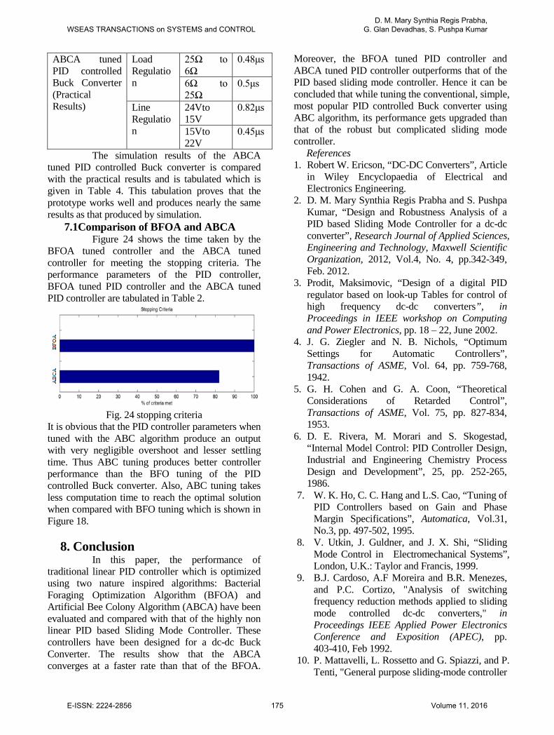
7.1Comparison of BFOA and ABCA Figure 24 shows the time taken by the BFOA tuned controller and the ABCA tuned controller for meeting the stopping criteria. The performance parameters of the PID controller, BFOA tuned PID controller and the ABCA tuned PID controller are tabulated in Table 2.

Fig. 24 stopping criteria

It is obvious that the PID controller parameters when tuned with the ABC algorithm produce an output with very negligible overshoot and lesser settling time. Thus ABC tuning produces better controller performance than the BFO tuning of the PID controlled Buck converter. Also, ABC tuning takes less computation time to reach the optimal solution when compared with BFO tuning which is shown in Figure 18.

8. Conclusion In this paper, the performance of traditional linear PID controller which is optimized using two nature inspired algorithms: Bacterial Foraging Optimization Algorithm (BFOA) and Artificial Bee Colony Algorithm (ABCA) have been evaluated and compared with that of the highly non linear PID based Sliding Mode Controller. These controllers have been designed for a dc-dc Buck Converter. The results show that the ABCA converges at a faster rate than that of the BFOA.

Moreover, the BFOA tuned PID controller and ABCA tuned PID controller outperforms that of the PID based sliding mode controller. Hence it can be concluded that while tuning the conventional, simple, most popular PID controlled Buck converter using ABC algorithm, its performance gets upgraded than that of the robust but complicated sliding mode controller.

References 1. Robert W. Ericson, “DC-DC Converters”, Article

in Wiley Encyclopaedia of Electrical and Electronics Engineering.

2. D. M. Mary Synthia Regis Prabha and S. Pushpa Kumar, “Design and Robustness Analysis of a PID based Sliding Mode Controller for a dc-dc converter”, Research Journal of Applied Sciences, Engineering and Technology, Maxwell Scientific Organization, 2012, Vol.4, No. 4, pp.342-349, Feb. 2012.

3. Prodit, Maksimovic, “Design of a digital PID regulator based on look-up Tables for control of high frequency dc-dc converters”, in Proceedings in IEEE workshop on Computing and Power Electronics, pp. 18 – 22, June 2002.

4. J. G. Ziegler and N. B. Nichols, “Optimum Settings for Automatic Controllers”, Transactions of ASME, Vol. 64, pp. 759-768, 1942.

5. G. H. Cohen and G. A. Coon, “Theoretical Considerations of Retarded Control”, Transactions of ASME, Vol. 75, pp. 827-834, 1953.

6. D. E. Rivera, M. Morari and S. Skogestad, “Internal Model Control: PID Controller Design, Industrial and Engineering Chemistry Process Design and Development”, 25, pp. 252-265, 1986.

7. W. K. Ho, C. C. Hang and L.S. Cao, “Tuning of PID Controllers based on Gain and Phase Margin Specifications”, Automatica, Vol.31, No.3, pp. 497-502, 1995.

8. V. Utkin, J. Guldner, and J. X. Shi, “Sliding Mode Control in Electromechanical Systems”, London, U.K.: Taylor and Francis, 1999.

9. B.J. Cardoso, A.F Moreira and B.R. Menezes, and P.C. Cortizo, "Analysis of switching frequency reduction methods applied to sliding mode controlled dc-dc converters," in Proceedings IEEE Applied Power Electronics Conference and Exposition (APEC), pp. 403-410, Feb 1992.

10. P. Mattavelli, L. Rossetto and G. Spiazzi, and P. Tenti, "General purpose sliding-mode controller



E-ISSN: 2224-2856 175 Volume 11, 2016

for dc/dc converter applications," in IEEE Power Electronics Specialists Conference Record (PESC), pp. 609--615, June 1993.

11. V. M. Nguyen and C.Q. Lee, "Indirect implementations of sliding-mode control law in buck-type converters”, in Proceedings, IEEE Applied Power Electronics Conference and Exposition (APEC), vol. 1, pp. 111-115, March 1996.

12. S.C. Tan, Y.M. Lai, C. K. Tse, and M.K.H. Cheung, "'A pulse-width-modulation based sliding mode controller for buck converters", in IEEE Power Electronics Specialists Conference Record (PESC 2004), pp. 3647-3653, June 2004.

13. Siew-Chong Tan, Y. M. Lai, and Chi K. Tse, “A Unified Approach to the Design of PWM-Based Sliding-Mode Voltage Controllers for Basic DC-DC Converters in Continuous Conduction Mode”, IEEE transactions on circuits and systems-I, Vol. 53, No. 8, pp. 1816-1827, Aug. 2006.

14. V. Rajinikanth and K. Latha, “Controller Parameter Optimization for Nonlinear Systems Using Enhanced Bacteria Foraging Algorithm”, Applied Computational Intelligence and Soft Computing, Vol. 2012, pp. 1-12, 2012.

15. OzdenErcin and RamazanCoban, “Comparison of the Artificial Bee Colony and the Bees Algorithm for PID Controller Tuning”, International Symposium on Innovation in Intelligent Systems and Applications, 2011, pp. 595-598.

16. O. T. Altinoz and H. Erdem, “Evaluation Function Comparison of Particle Swarm Optimization for Buck Converter”, International Symposium on Power Electronics, Electrical Drives, Automation and Motion, 2010, pp. 798-802.

17. H. Vahedi, S. H. Hosseini and R. Noroozian, “Bacterial Foraging Algorithm for security constrained optimal power flow”, 7th International Conference on the European Energy Market, 2010, pp. 1-6

18. A. Jalilvand, H. Vahedi and A. Bayat, “Optimal Tuning of the PID Controller for a Buck Converter using Bacterial Foraging Algorithm”, Intelligent and Advanced Systems (ICIAS), 2010, pp. 1-5

19. M. Abachizadeh, M.R.H. Yazdi and A. Yousefi-Koma, “Optimal tuning of PID controllers using Artificial Bee Colony algorithm”, IEEE International Conference on

Advanced Intelligent Mechatronics (AIM), 2010.

20. Karl J. Astrom, Tore Hagglund, “PID Controllers”, second edition, Instrument Society of India, pp.164,1995.

21. Passino, K. M., “Biomimicry of Bacterial Foraging for Distributed Optimization and Control”, IEEE Control Systems Magazine, 52-67, June 2002.

22. Liu Yanfei and Passino, K. M., “Biomimicry of Social Foraging Bacteria for Distributed Optimization: Models, Principles, and Emergent Behaviors”, Journal of Optimization Theory And Applications, Vol. 115, No. 3, pp. 603–628, Dec. 2002.

23. Passino, K.M., "Bacterial Foraging Optimization," Int. J. Swarm Intelligence Research, Vol. 1, No. 1, pp. 1-16, Jan.-March, 2010.

24. Swagatam Das, ArijitBiswas, SambartaDasgupta, and Ajith Abraham, “The Bacterial Foraging Optimization – Algorithm, Analysis, and Applications, Foundations on Computational Intelligence”, Aboul-Ella Hassanien and Ajith Abraham Eds., Studies in Computational Intelligence, Springer Verlag, Germany, 2008.

25. Das Swagatam, DasguptaSambarta, BiswasArijit, Abraham Ajith and KonarAmit, “On stability of the chemotactic dynamics in bacterial-foraging optimization algorithm”, IEEE Trans Syst Man Cyber – Part A: Syst Humans, Vol. 39, No.3, 2009.

26. D. M. Mary Synthia Regis Prabha, G. GlanDevadhas, “An Optimum Setting of Controller for a dc-dc converter Using Bacterial Intelligence Technique”, Innovative soft grid technologies-India (ISGT-India), IEEE 2011, PES, pp. 204-210, 2011.

27. D.T. Pham, A. Ghanbarzadeh, E. Koc, S. Otri, S. Rahim and M. Zaidi, “The bees algorithm”, Technical Report, Manufacturing Engineering Centre, Cardiff University, UK, 2005.

28. D. Karaboga, “An idea based on honey bee swarm for numerical optimization”, Technical Report TR06, Erciyes University, Engineering Faculty, Computer Engineering Department, 2005.



E-ISSN: 2224-2856 176 Volume 11, 2016

http://www.researchgate.net/researcher/74644808_M_Abachizadeh/

http://www.researchgate.net/researcher/74862556_MRH_Yazdi/

http://www.researchgate.net/researcher/75118910_A_Yousefi-Koma/



Documents

Optimum Setting and Performance Evaluation of the … · Optimum Setting and Performance Evaluation of the Three Mode Controller Using Bio Inspired Soft Computing Algorithms