Optimizing Pattern Recognition Systems

Professor Mike Manry

University of Texas at Arlington

Introduction Feature SelectionComplexity MinimizationRecent Classification Technologies

Neural NetsSupport Vector MachinesBoosting

A Maximal Margin ClassifierGrowing and PruningSoftwareExamplesConclusions

Outline

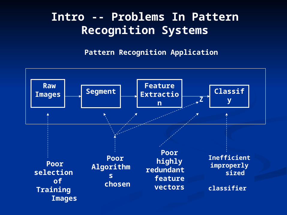
Intro -- Problems In Pattern Recognition Systems

Segment Raw

ImagesFeature

Extraction Classify

Poor selection of Training

Images

Pattern Recognition Application

Inefficientimproperly

sized classifier

PoorAlgorithms chosen

Poor highly

redundant feature vectors

Z

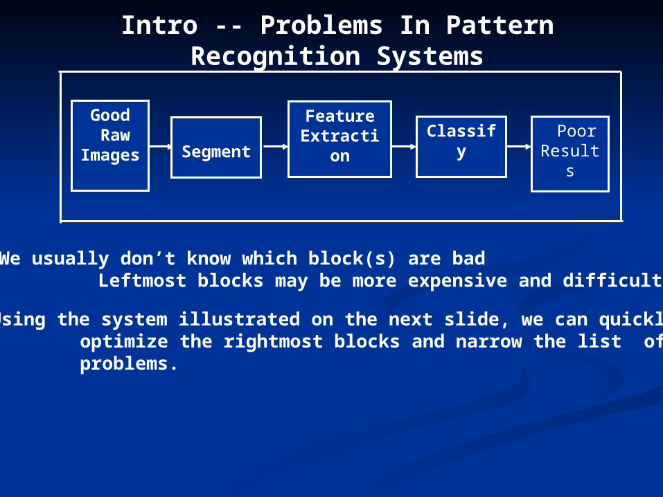
Intro -- Problems In Pattern Recognition Systems

Problems: We usually don’t know which block(s) are bad Leftmost blocks may be more expensive and difficult to change

Good Raw

Images

FeatureExtraction Classify Poor

ResultsSegment

Solution: Using the system illustrated on the next slide, we can quickly optimize the rightmost blocks and narrow the list of potential problems.

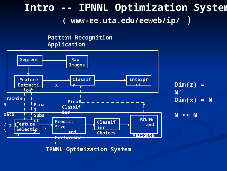
Intro -- IPNNL Optimization System( www-ee.uta.edu/eeweb/ip/ )

Segment RawImages

FeatureExtraction

Classify Interpret

FeatureSelection

Predict Size and Performance

ClassifierChoices

Training Data { z,ic }

FinalSubset x

x

x

Prune and Validate

FinalClassifier

Pattern Recognition Application

IPNNL Optimization System

Dim(z) = N’ Dim(x) = N N << N’

Intro -- Presentation Goals

Examine blocks in the Optimization System:

• Feature Selection• Recent Classification Technologies• Growing and Pruning of Neural Net Classifiers

Demonstrate the Optimization System on:

• Data from Bell Helicopter Textron• Data from UTA Bioengineering• Data from UTA Civil Engineering

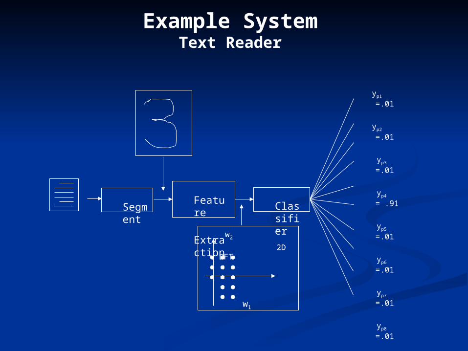
Feature

Extraction Segment

w2

2D DFT

w1

Classifier

yp1 =.01

yp2 =.01

yp3 =.01

yp4 = .91

yp5 =.01

yp6 =.01

yp7 =.01

yp8 =.01

yp9 =.01

yp10 =.01

Example SystemText Reader

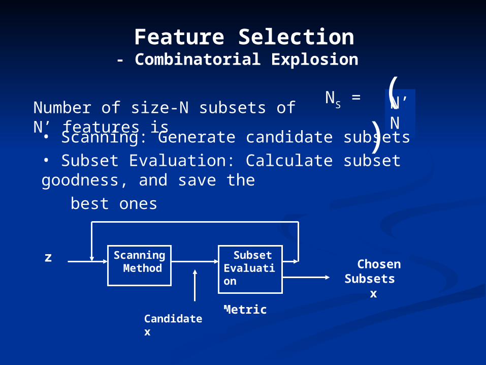
Feature Selection- Combinatorial Explosion

Number of size-N subsets of N’ features isN’NNS = ( )

Scanning Method

z Subset Evaluation Metric

Candidate x

Chosen Subsets x

• Scanning: Generate candidate subsets

• Subset Evaluation: Calculate subset goodness, and save the

best ones

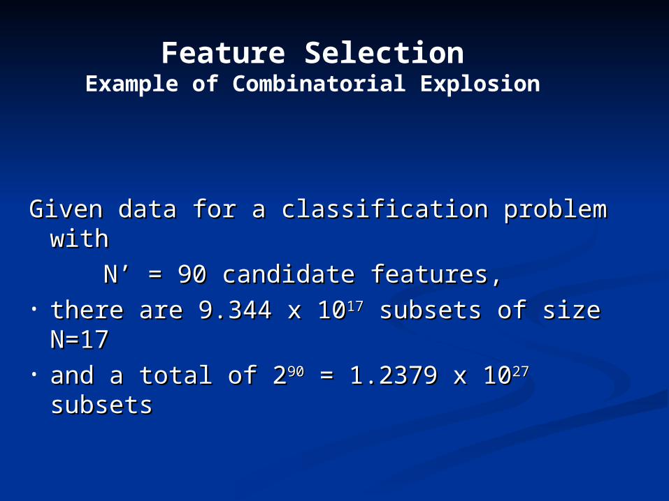
Given data for a classification problem with Given data for a classification problem with

N’ = 90 candidate features,N’ = 90 candidate features,• there are 9.344 x 10there are 9.344 x 101717 subsets of size N=17 subsets of size N=17 • and a total of 2and a total of 29090 = 1.2379 x 10 = 1.2379 x 102727 subsets subsets

Feature SelectionExample of Combinatorial Explosion

Feature Selection- Scanning Methods

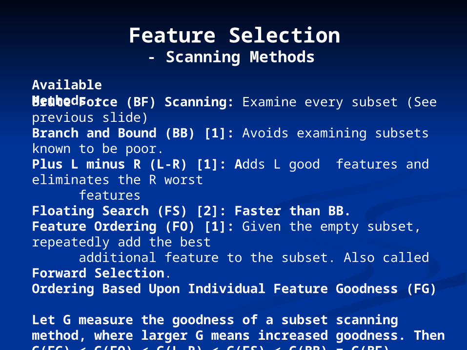
Available Methods :

Brute Force (BF) Scanning: Examine every subset (See previous slide)Branch and Bound (BB) [1]: Avoids examining subsets known to be poor.Plus L minus R (L-R) [1]: Adds L good features and eliminates the R worst featuresFloating Search (FS) [2]: Faster than BB. Feature Ordering (FO) [1]: Given the empty subset, repeatedly add the best additional feature to the subset. Also called Forward Selection. Ordering Based Upon Individual Feature Goodness (FG)

Let G measure the goodness of a subset scanning method, where larger G means increased goodness. ThenG(FG) < G(FO) < G(L-R) < G(FS) < G(BB) = G(BF)

Feature Selection Scanning Methods: Feature Goodness vs. Brute Force

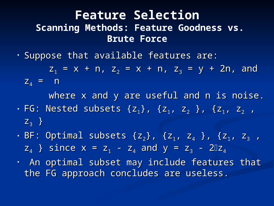
• Suppose that available features are:Suppose that available features are:

zz11 = x + n, z = x + n, z22 = x + n, z = x + n, z33 = y + 2n, and z = y + 2n, and z44 = n = n

where x and y are useful and n is noise.where x and y are useful and n is noise.• FG: Nested subsets {zFG: Nested subsets {z11}, {z}, {z11, z, z22 }, {z }, {z11, z, z22 , z , z33 } }

• BF: Optimal subsets {zBF: Optimal subsets {z22}, {z}, {z11, z, z44 }, {z }, {z11, z, z33 , z , z44 } }

since x = zsince x = z11 - z - z44 and y = z and y = z33 - 2 - 2zz44

• An optimal subset may include features that the An optimal subset may include features that the FG approach concludes are useless. FG approach concludes are useless.

Feature Selection- Subset Evaluation Metrics (SEMs)

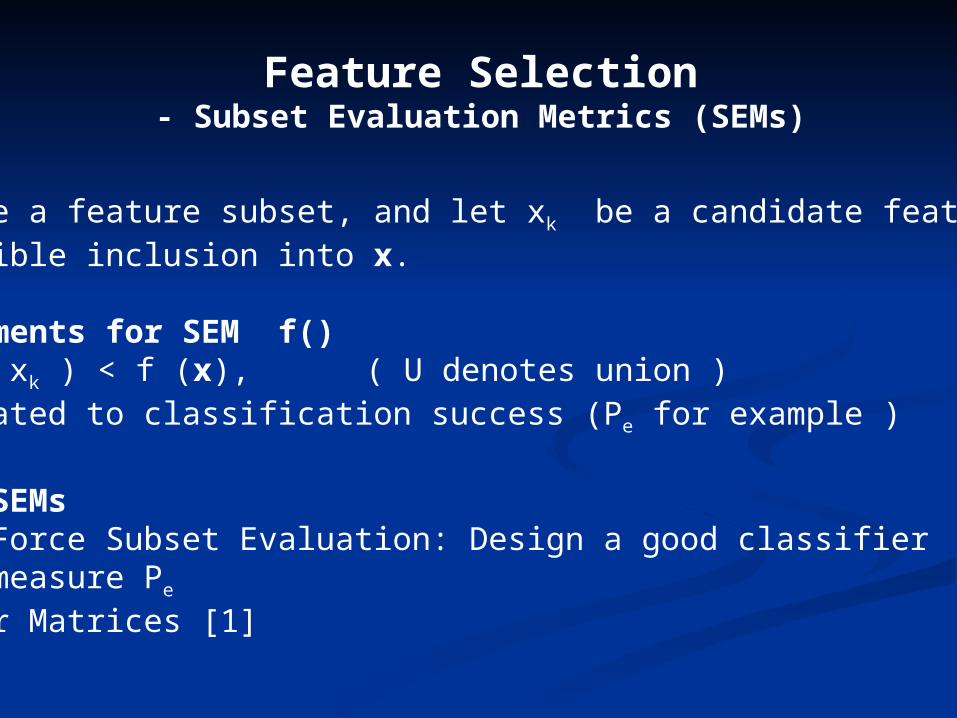
Let x be a feature subset, and let xk be a candidate feature for possible inclusion into x.

Requirements for SEM f()•f ( x U xk ) < f (x), ( U denotes union )•f() related to classification success (Pe for example )

Example SEMs • Brute Force Subset Evaluation: Design a good classifier and measure Pe

• Scatter Matrices [1]

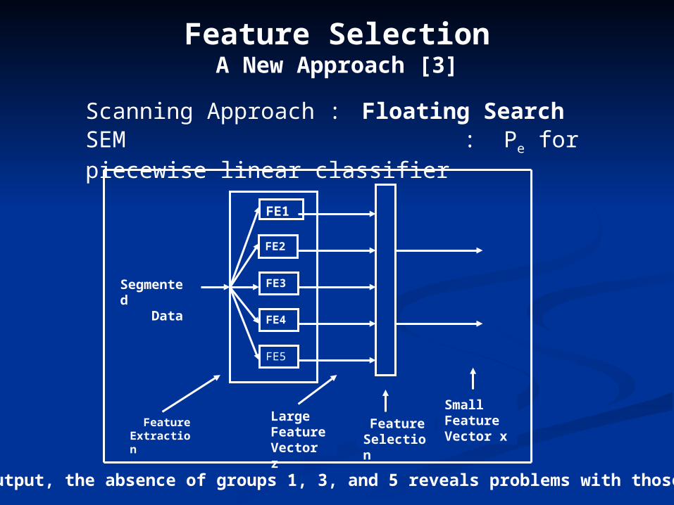
Feature SelectionA New Approach [3]

Scanning Approach : Floating Search SEM : Pe for piecewise linear classifier

Segmented Data

Feature Extraction

FE5

FE1

FE4

FE3

FE2

Feature Selection

LargeFeature Vector z

SmallFeatureVector x

At the output, the absence of groups 1, 3, and 5 reveals problems with those groups

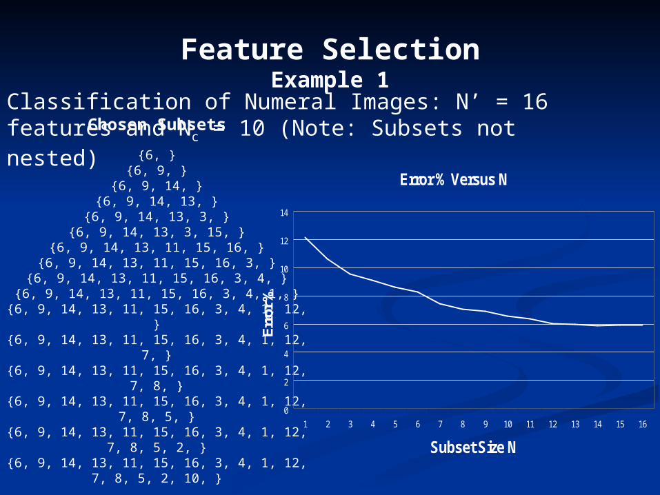
Feature SelectionExample 1

Classification of Numeral Images: N’ = 16 features and Nc = 10 (Note: Subsets not nested)

Chosen Subsets

{6, }{6, 9, }

{6, 9, 14, }{6, 9, 14, 13, }

{6, 9, 14, 13, 3, }{6, 9, 14, 13, 3, 15, }

{6, 9, 14, 13, 11, 15, 16, }{6, 9, 14, 13, 11, 15, 16, 3, }

{6, 9, 14, 13, 11, 15, 16, 3, 4, }{6, 9, 14, 13, 11, 15, 16, 3, 4, 1, }

{6, 9, 14, 13, 11, 15, 16, 3, 4, 1, 12, }{6, 9, 14, 13, 11, 15, 16, 3, 4, 1, 12, 7, }

{6, 9, 14, 13, 11, 15, 16, 3, 4, 1, 12, 7, 8, }{6, 9, 14, 13, 11, 15, 16, 3, 4, 1, 12, 7, 8, 5, }

{6, 9, 14, 13, 11, 15, 16, 3, 4, 1, 12, 7, 8, 5, 2, }{6, 9, 14, 13, 11, 15, 16, 3, 4, 1, 12, 7, 8, 5, 2, 10, }

Error % Versus N

0

2

4

6

8

10

12

14

1 2 3 4 5 6 7 8 9 10 11 12 13 14 15 16

Subset Size N

Erro

r %

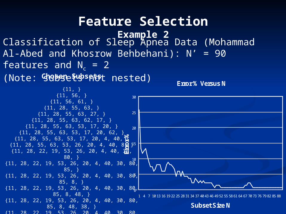
Feature SelectionExample 2

Error % Versus N

0

5

10

15

20

25

30

1 4 7 10 13 16 19 22 25 28 31 34 37 40 43 46 49 52 55 58 61 64 67 70 73 76 79 82 85 88

Subset Size N

Err

or

%

Classification of Sleep Apnea Data (Mohammad Al-Abed and Khosrow Behbehani): N’ = 90 features and Nc = 2(Note: subsets not nested)

Chosen Subsets

{11, }{11, 56, }

{11, 56, 61, }{11, 28, 55, 63, }

{11, 28, 55, 63, 27, }{11, 28, 55, 63, 62, 17, }

{11, 28, 55, 63, 53, 17, 20, }{11, 28, 55, 63, 53, 17, 20, 62, }

{11, 28, 55, 63, 53, 17, 20, 4, 40, }{11, 28, 55, 63, 53, 26, 20, 4, 40, 8, }

{11, 28, 22, 19, 53, 26, 20, 4, 40, 30, 80, }{11, 28, 22, 19, 53, 26, 20, 4, 40, 30, 80, 85, }

{11, 28, 22, 19, 53, 26, 20, 4, 40, 30, 80, 85, 8, }{11, 28, 22, 19, 53, 26, 20, 4, 40, 30, 80, 85, 8, 48, }

{11, 28, 22, 19, 53, 26, 20, 4, 40, 30, 80, 85, 8, 48, 38, }{11, 28, 22, 19, 53, 26, 20, 4, 40, 30, 80, 85, 8, 48, 45, 87, }

{11, 28, 13, 19, 53, 26, 65, 4, 40, 30, 80, 85, 8, 48, 75, 87, 18, }

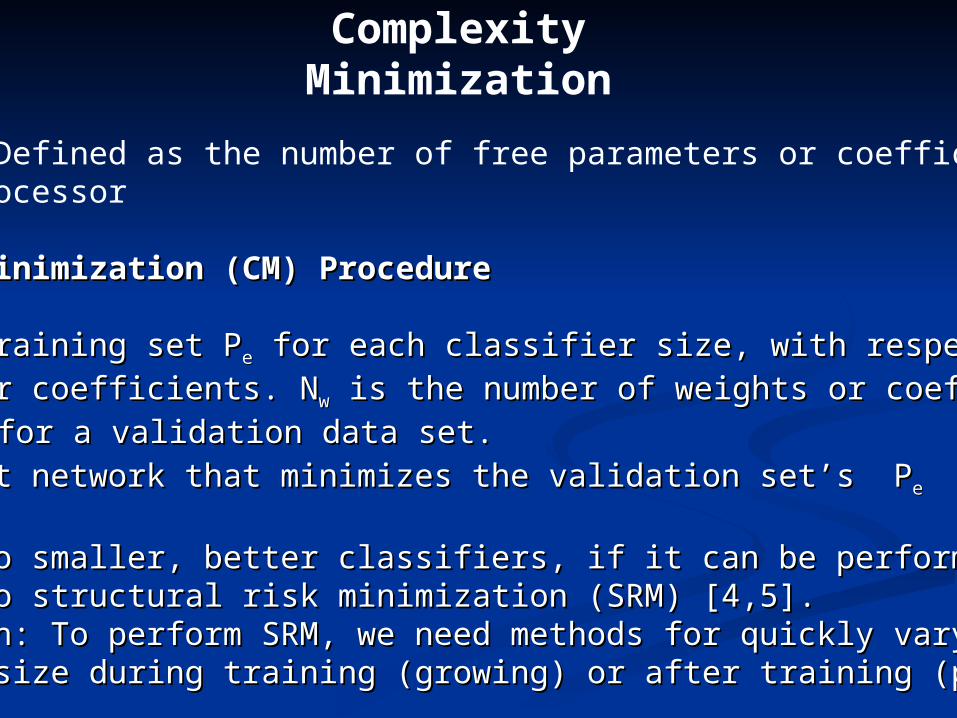
Complexity Minimization

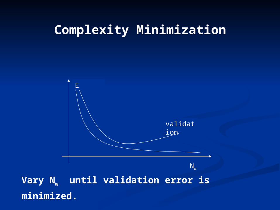
Complexity: Defined as the number of free parameters or coefficients in a processor

Complexity Minimization (CM) ProcedureComplexity Minimization (CM) Procedure

• Minimize training set PMinimize training set Pee for each classifier size, with respect to all for each classifier size, with respect to all

weights or coefficients. Nweights or coefficients. Nww is the number of weights or coefficients. is the number of weights or coefficients. • Measure PMeasure Pe e for a validation data set.for a validation data set.• Choose that network that minimizes the validation set’s PChoose that network that minimizes the validation set’s Pee

• CM leads to smaller, better classifiers, if it can be performed. It is CM leads to smaller, better classifiers, if it can be performed. It is related to structural risk minimization (SRM) [4,5].related to structural risk minimization (SRM) [4,5].• Implication: To perform SRM, we need methods for quickly varying Implication: To perform SRM, we need methods for quickly varying network size during training (growing) or after training (pruning)network size during training (growing) or after training (pruning)

Complexity Minimization

E

Nw

validation

Vary Nw until validation error is minimized.

Recent Classification TechnologiesNeural Nets

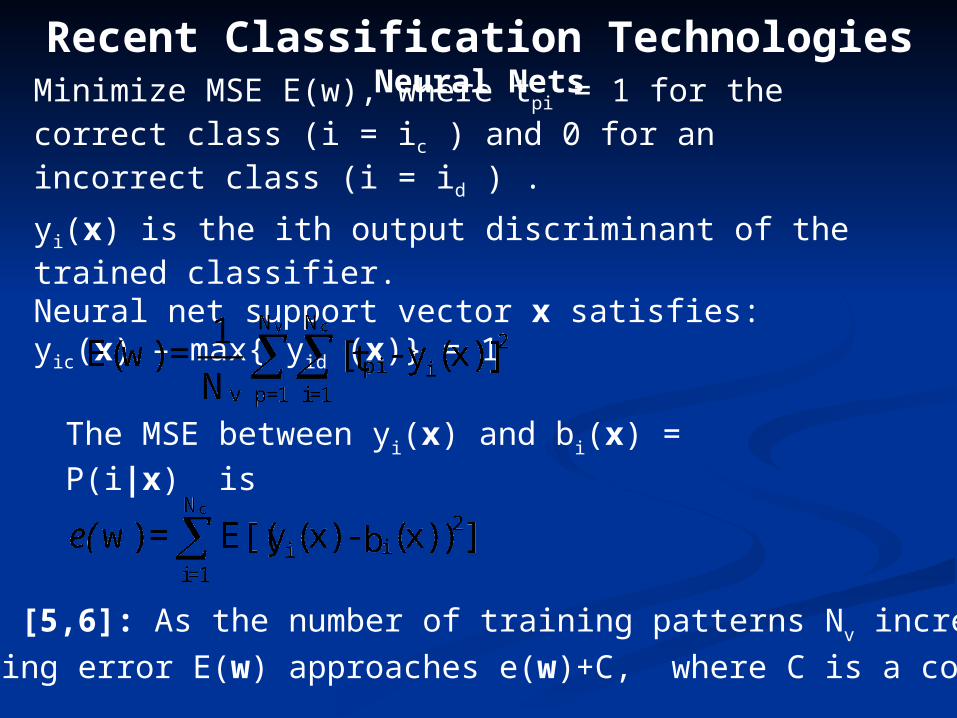
Minimize MSE E(w), where tpi = 1 for the correct class (i = ic ) and 0 for an incorrect class (i = id ) .

yi(x) is the ith output discriminant of the trained classifier. Neural net support vector x satisfies: yic(x) – max{ yid (x)} = 1

The MSE between yi(x) and bi(x) = P(i|x) is

Theorem 1 [5,6]: As the number of training patterns Nv increases,

the training error E(w) approaches e(w)+C, where C is a constant.

Recent Classification TechnologiesNeural Nets

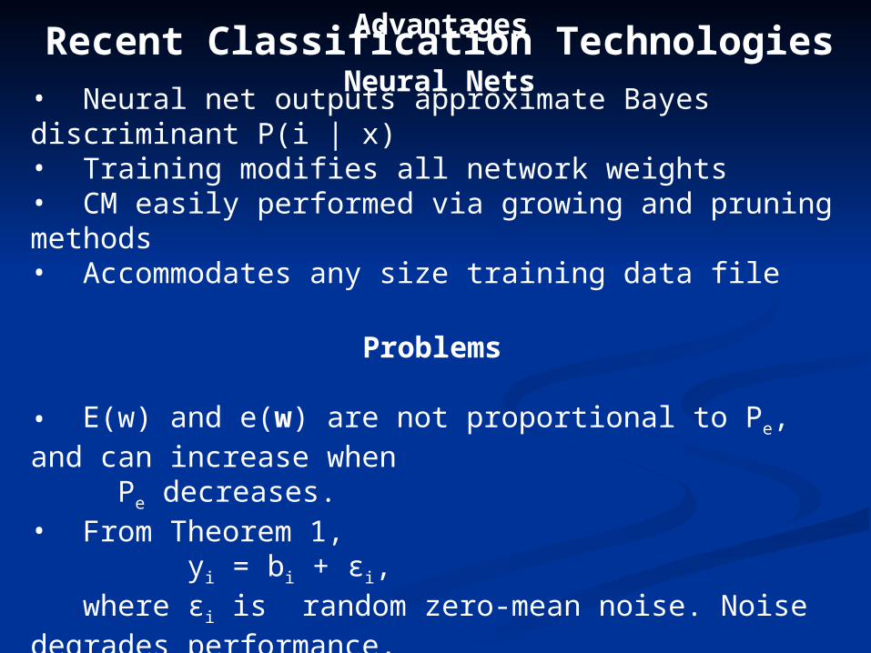
Advantages

• Neural net outputs approximate Bayes discriminant P(i | x)• Training modifies all network weights• CM easily performed via growing and pruning methods• Accommodates any size training data file

Problems

• E(w) and e(w) are not proportional to Pe, and can increase when Pe decreases.• From Theorem 1, yi = bi + εi, where εi is random zero-mean noise. Noise degrades performance, leaving room for improvement via SVM training and boosting.

Recent Classification Technologies Support Vector Machines [4,5]

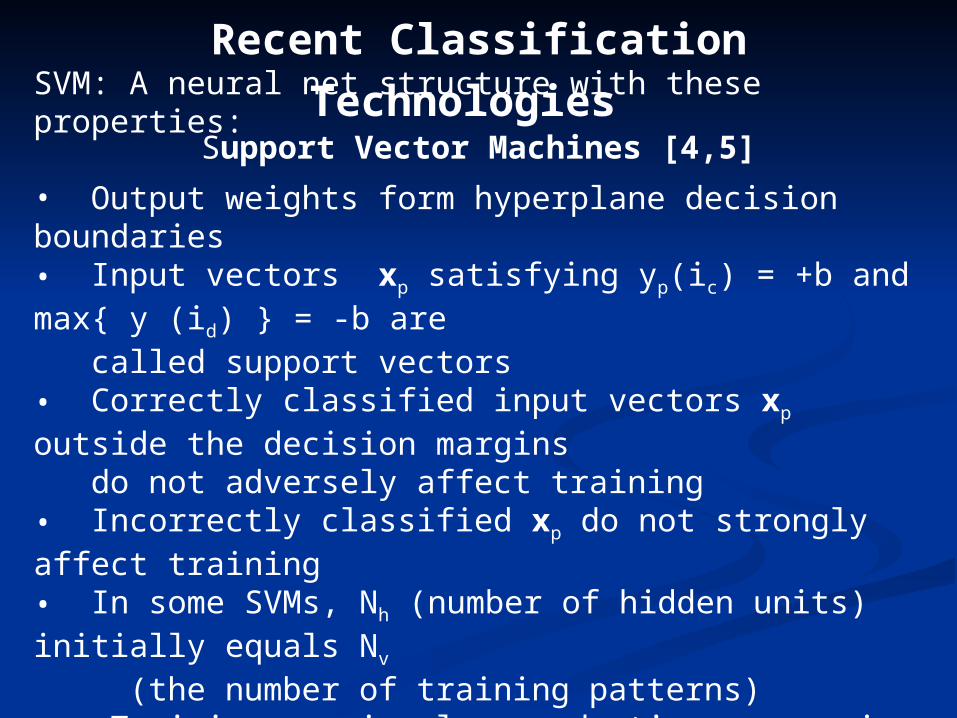
SVM: A neural net structure with these properties:

• Output weights form hyperplane decision boundaries• Input vectors xp satisfying yp(ic) = +b and max{ y (id) } = -b are called support vectors • Correctly classified input vectors xp outside the decision margins do not adversely affect training• Incorrectly classified xp do not strongly affect training• In some SVMs, Nh (number of hidden units) initially equals Nv

(the number of training patterns) • Training may involve quadratic programming

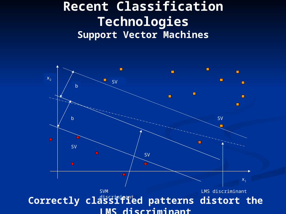
b

b

SVM discriminant LMS discriminant

x2

x1

SV

SV

SV

SV

Correctly classified patterns distort the LMS discriminant

Recent Classification TechnologiesSupport Vector Machines

Recent Classification TechnologiesSupport Vector Machines

Advantage: Good classifiers from small data sets

Problems

• SVM design methods are practical only for small data sets• Training difficult when there are many classes• Kernel parameter found by hit or miss • Fails to minimize complexity (far too many hidden units required, input weights don’t adapt) [7] Current Work

• Modelling SVMs with much smaller neural nets. • Developing Regression-based maximal margin classifiers

Recent Classification TechnologiesBoosting [5]

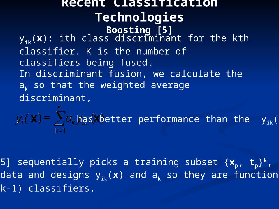
yik(x): ith class discriminant for the kth classifier. K is the

number of classifiers being fused.In discriminant fusion, we calculate the ak so that the

weighted average discriminant,

Adaboost [5] sequentially picks a training subset {xp, tp}k, from the available data and designs yik(x) and ak so they are functions of the

previous (k-1) classifiers.

has better performance than the yik(x)

Recent Classification TechnologiesBoosting

Advantage

• Final classifier can be used to process video signals in real time when step function activations are used

Problems• Works best for the two-class case, uses huge data files.• Final classifier is a large, highly redundant neural net.• Training can take days, CM not performed.

Future Work

• Pruning and modelling should be tried to reduce redundancy.• Feature selection should be tried to speed up training

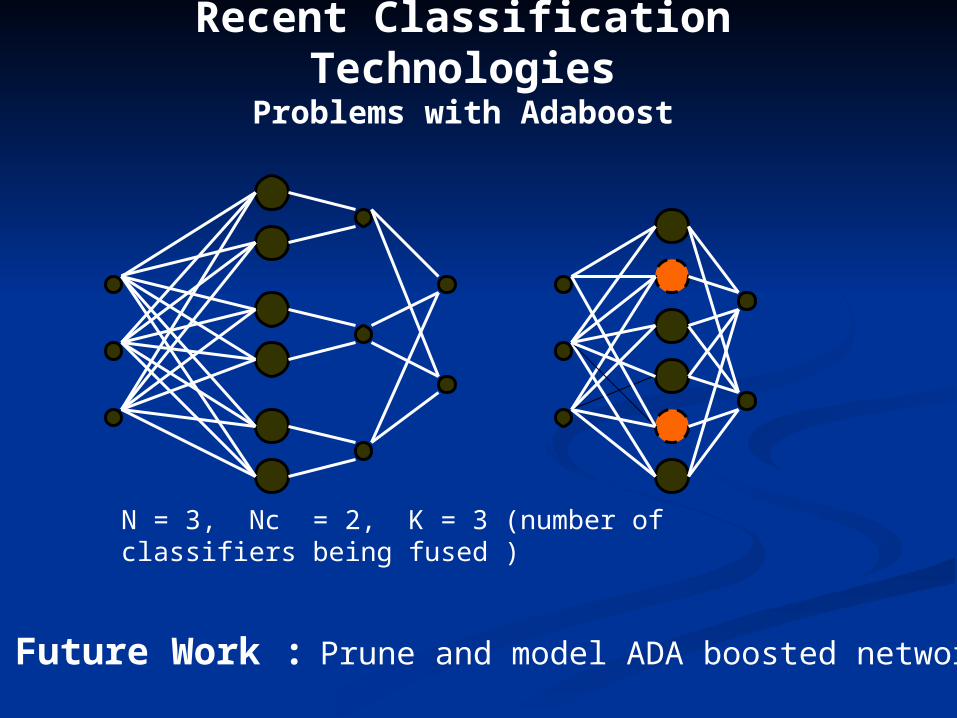
Recent Classification TechnologiesProblems with Adaboost

Future Work : Prune and model ADA boosted networks

N = 3, Nc = 2, K = 3 (number of classifiers being fused )

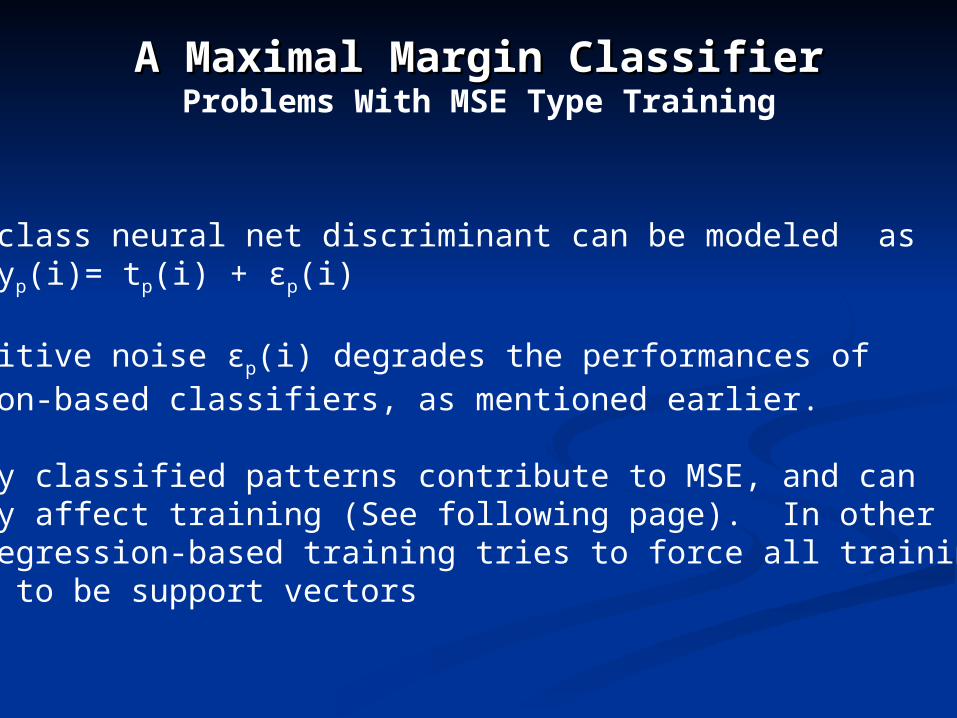
A Maximal Margin ClassifierA Maximal Margin ClassifierProblems With MSE Type Training

The ith class neural net discriminant can be modeled as yp(i)= tp(i) + εp(i)

This additive noise εp(i) degrades the performances of regression-based classifiers, as mentioned earlier.

Correctly classified patterns contribute to MSE, and can adversely affect training (See following page). In other words, regression-based training tries to force all training patterns to be support vectors

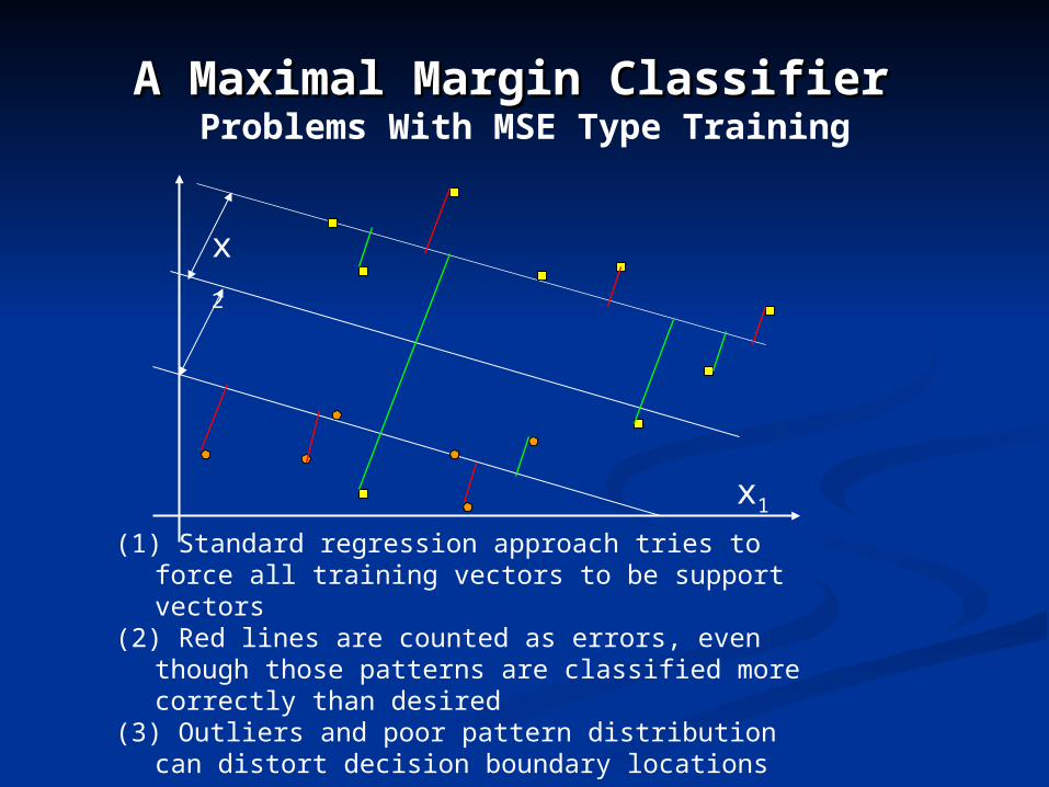
A Maximal Margin Classifier A Maximal Margin Classifier Problems With MSE Type Training

(1) Standard regression approach tries to force all training vectors to be support vectors

(2) Red lines are counted as errors, even though those patterns are classified more correctly than desired

(3) Outliers and poor pattern distribution can distort decision boundary locations

x1

x2

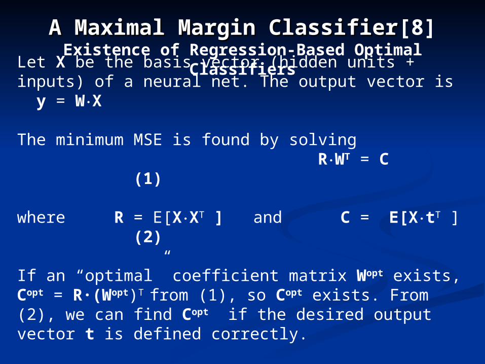
A Maximal Margin ClassifierA Maximal Margin Classifier[8]Existence of Regression-Based Optimal Classifiers

Let X be the basis vector (hidden units + inputs) of a neural net. The output vector is y = W·X

The minimum MSE is found by solving R·WT = C (1)

where R = E[X·XT ] and C = E[X·tT ] (2)

If an “optimal” coefficient matrix Wopt exists, Copt = R·(Wopt)T from (1), so Copt exists. From (2), we can find Copt if the desired output vector t is defined correctly.

Regression-based training can mimic other approaches.

A Maximal Margin ClassifierA Maximal Margin Classifier Regression Based Classifier Design [8]

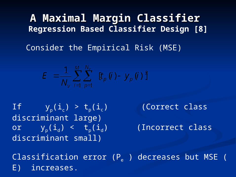
Consider the Empirical Risk (MSE)

If yp(ic) > tp(ic) (Correct class discriminant large)

or yp(id) < tp(id) (Incorrect class discriminant small)

Classification error (Pe ) decreases but MSE ( E) increases.

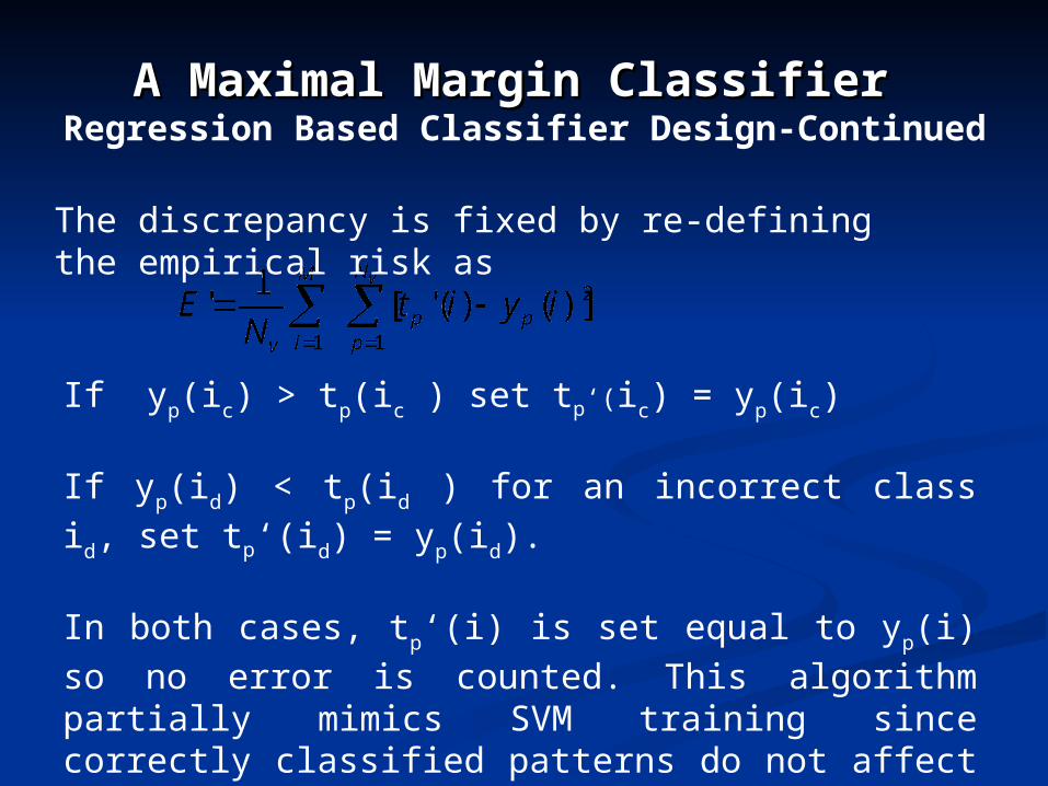
If yp(ic) > tp(ic ) set tp‘(ic) = yp(ic)

If yp(id) < tp(id ) for an incorrect class id, set tp‘(id) = yp(id).

In both cases, tp‘(i) is set equal to yp(i) so no error is counted.

This algorithm partially mimics SVM training since correctly classified patterns do not affect the MSE too much.( Related to Ho-Kashyap procedures, [5] pp.249-256 )

The discrepancy is fixed by re-defining the empirical risk as 

A Maximal Margin ClassifierA Maximal Margin Classifier Regression Based Classifier Design-Continued

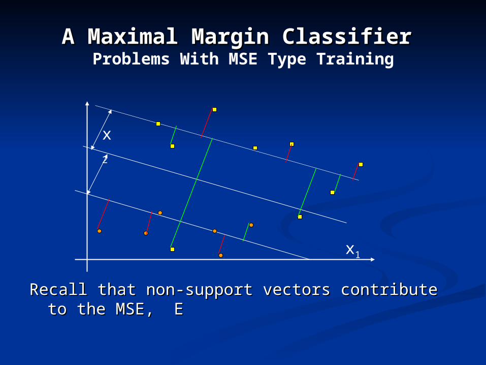
A Maximal Margin Classifier A Maximal Margin Classifier Problems With MSE Type Training

x1

x2

Recall that non-support vectors contribute to the MSE, ERecall that non-support vectors contribute to the MSE, E

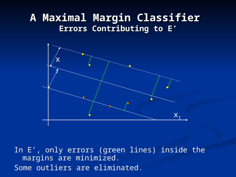
A Maximal Margin ClassifierA Maximal Margin Classifier Errors Contributing to E’Errors Contributing to E’

In E’, only errors (green lines) inside the margins are minimized. Some outliers are eliminated.

x1

x2

A Maximal Margin ClassifierA Maximal Margin Classifier CommentsComments

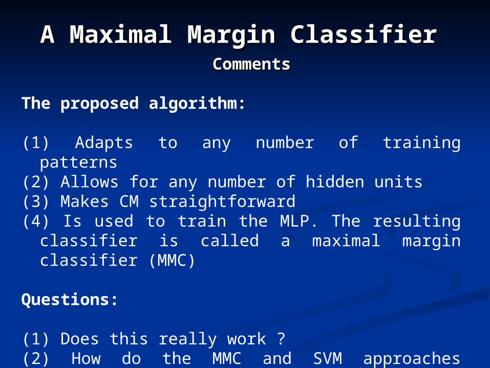
The proposed algorithm: (1) Adapts to any number of training patterns(2) Allows for any number of hidden units(3) Makes CM straightforward(4) Is used to train the MLP. The resulting classifier is called a

maximal margin classifier (MMC)

Questions:

(1) Does this really work ?(2) How do the MMC and SVM approaches compare ?

A Maximal Margin ClassifierA Maximal Margin Classifier Two-Class Example

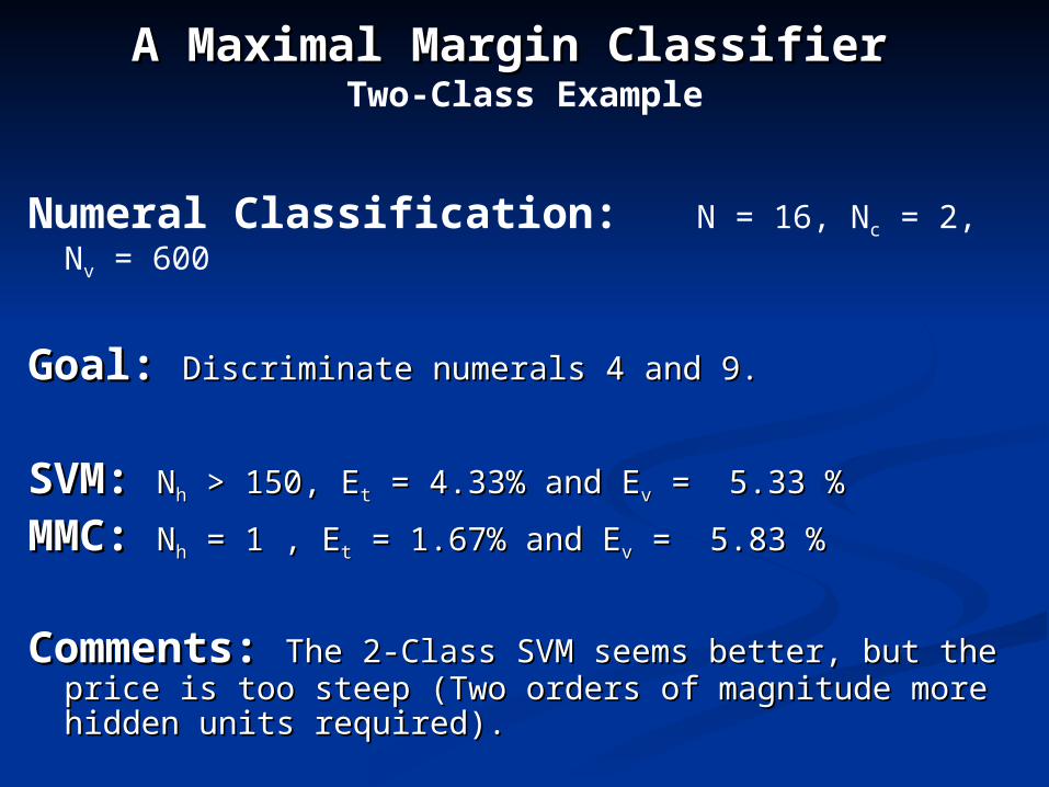
Numeral Classification: N = 16, Nc = 2, Nv = 600

Goal:Goal: Discriminate numerals 4 and 9.Discriminate numerals 4 and 9.

SVM:SVM: NNhh > 150, E > 150, Ett = 4.33% and E = 4.33% and Evv = 5.33 % = 5.33 %

MMC:MMC: NNhh = 1 , E = 1 , Ett = 1.67% and E = 1.67% and Evv = 5.83 % = 5.83 %

Comments:Comments: The 2-Class SVM seems better, but the price is too The 2-Class SVM seems better, but the price is too steep (Two orders of magnitude more hidden units required).steep (Two orders of magnitude more hidden units required).

A Maximal Margin ClassifierA Maximal Margin Classifier Multi-Class Examples

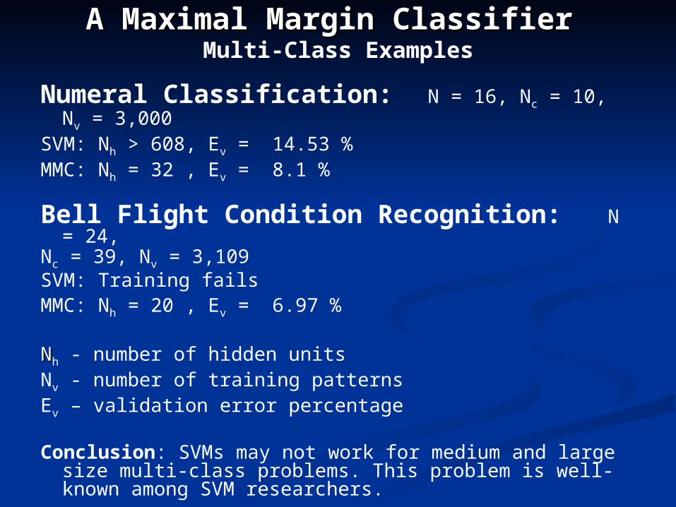
Numeral Classification: N = 16, Nc = 10, Nv = 3,000

SVM: Nh > 608, Ev = 14.53 % MMC: Nh = 32 , Ev = 8.1 %

Bell Flight Condition Recognition: N = 24, Nc = 39, Nv = 3,109SVM: Training failsMMC: Nh = 20 , Ev = 6.97 %

NNh - number of hidden unitsNv - number of training patternsEv – validation error percentage

Conclusion: SVMs may not work for medium and large size multi-class problems. This problem is well-known among SVM researchers.

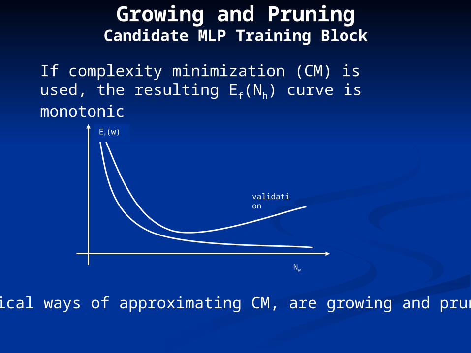
Growing and PruningCandidate MLP Training Block

If complexity minimization (CM) is used, the resulting Ef(Nh) curve is monotonic

Ef(w)

Nw

validation

Practical ways of approximating CM, are growing and pruning.

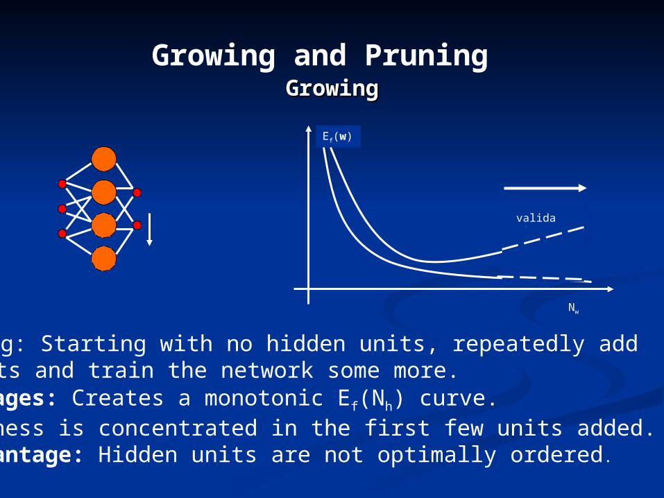
Growing and Pruning GrowingGrowing

Ef(w)

Nw

validation

Growing: Starting with no hidden units, repeatedly add Na units and train the network some more. Advantages: Creates a monotonic Ef(Nh) curve. Usefulness is concentrated in the first few units added.Disadvantage: Hidden units are not optimally ordered.

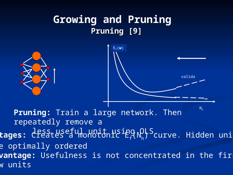
Growing and Pruning Pruning [9]Pruning [9]

Ef(w)

Nw

validation

Pruning: Train a large network. Then repeatedly remove a less useful unit using OLS. Advantages: Creates a monotonic Ef(Nh) curve. Hidden units

are optimally orderedDisadvantage: Usefulness is not concentrated in the first few units

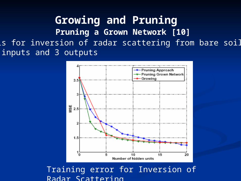
Growing and Pruning Pruning a Grown Network [10]

Training error for Inversion of Radar Scattering

Data set is for inversion of radar scattering from bare soil surfaces. It has 20 inputs and 3 outputs

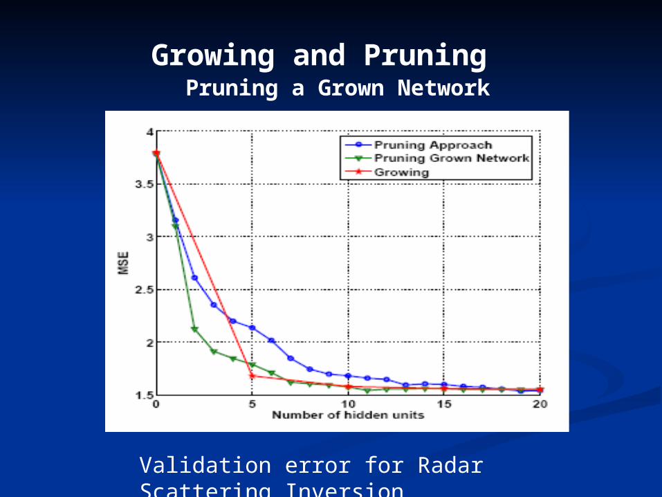
Growing and Pruning Pruning a Grown Network

Validation error for Radar Scattering Inversion

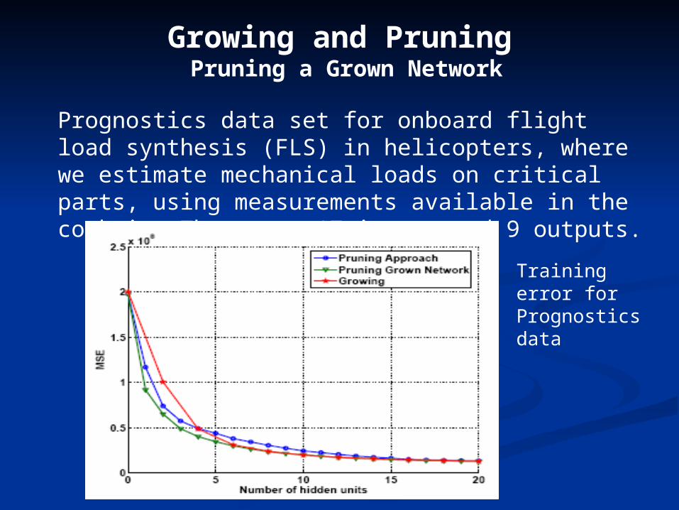
Growing and Pruning Pruning a Grown Network

Prognostics data set for onboard flight load synthesis (FLS) in helicopters, where we estimate mechanical loads on critical parts, using measurements available in the cockpit. There are 17 inputs and 9 outputs.

Training error for Prognostics data

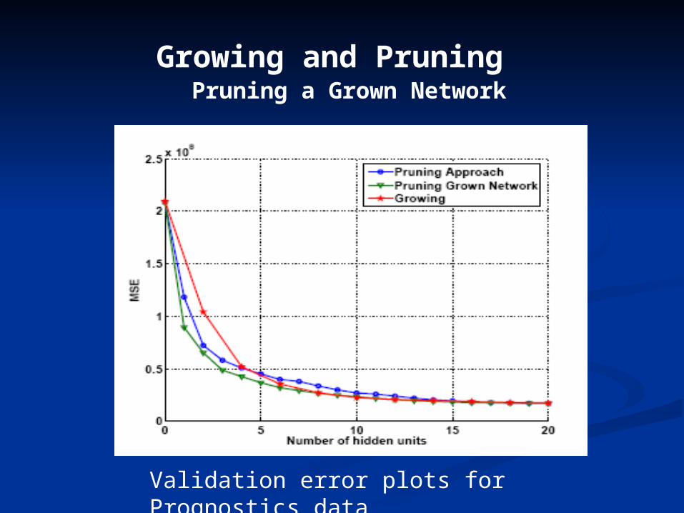
Growing and Pruning Pruning a Grown Network

Validation error plots for Prognostics data

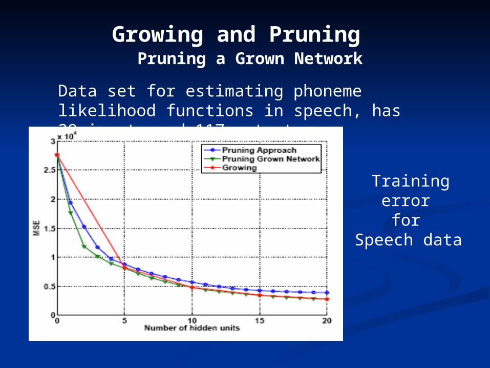
Growing and Pruning Pruning a Grown Network

Data set for estimating phoneme likelihood functions in speech, has 39 inputs and 117 outputs

Training error for

Speech data

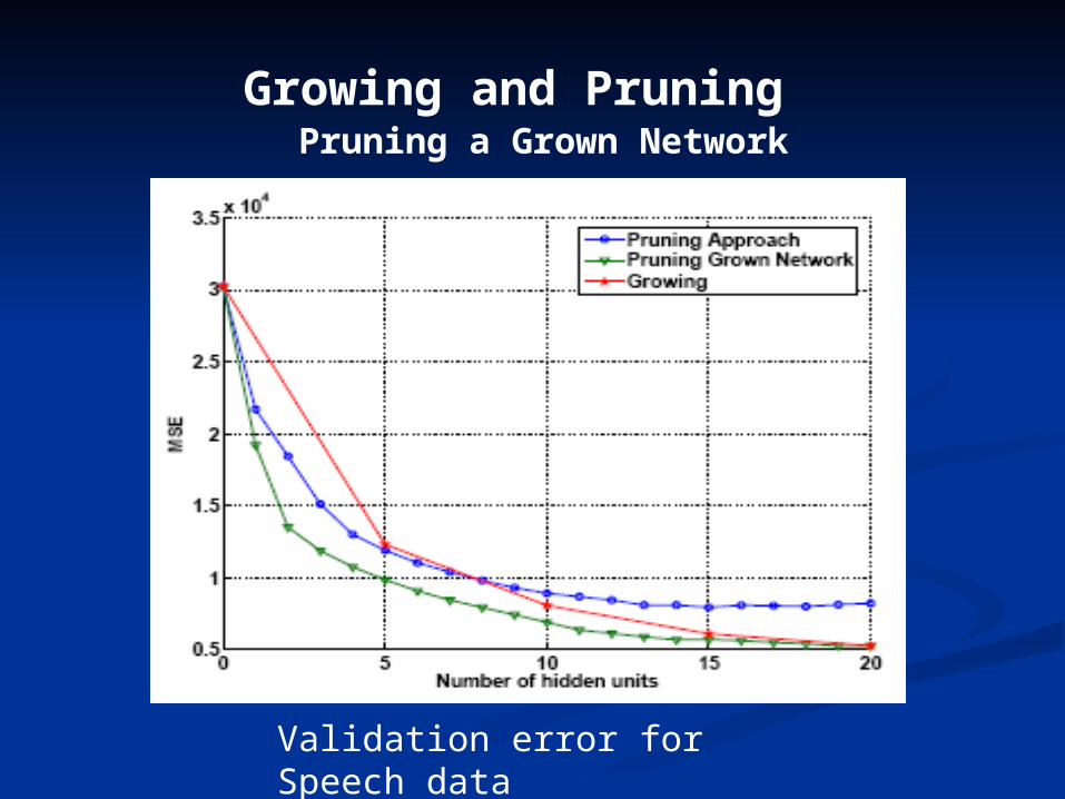
Growing and Pruning Pruning a Grown Network

Validation error for Speech data

• Remaining Work: Insert into the Remaining Work: Insert into the IPNNL Optimization System

Growing and Pruning

IPNNL SoftwareMotivation

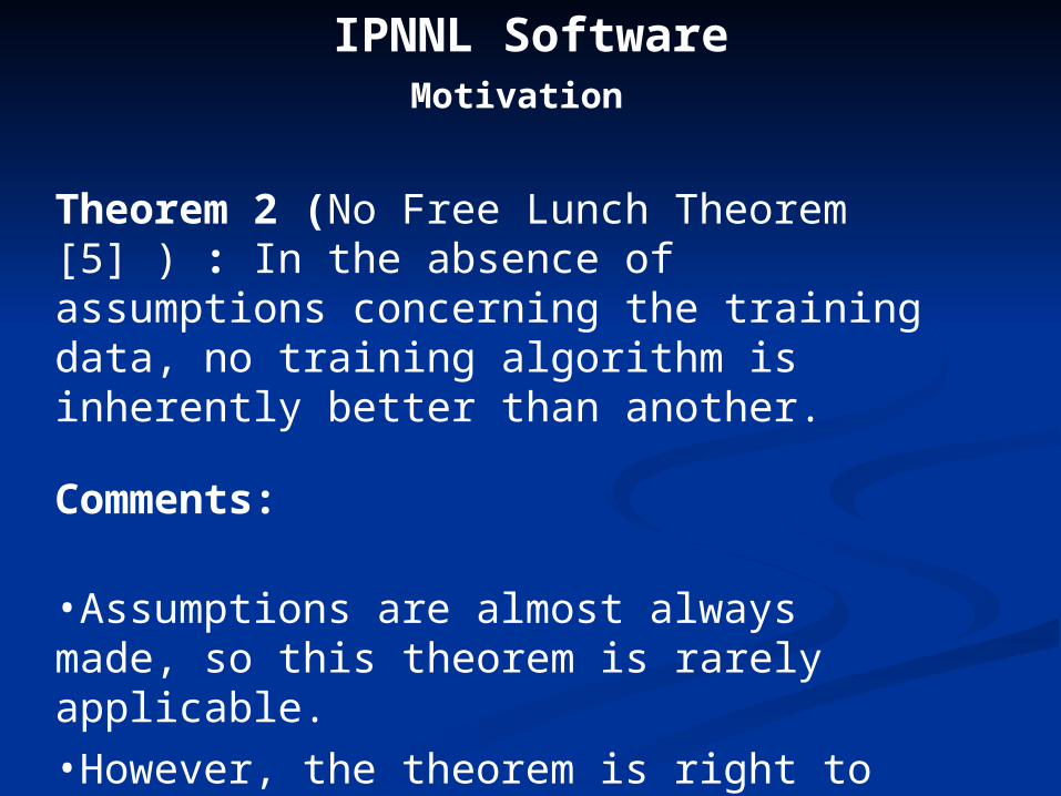
Theorem 2 (No Free Lunch Theorem [5] ) : In the absence of assumptions concerning the training data, no training algorithm is inherently better than another.

Comments:

•Assumptions are almost always made, so this theorem is rarely applicable.

•However, the theorem is right to the extent that given training data, several classifiers should be tried after feature selection.

IPNNL Software Block DiagramBlock Diagram

Size TrainPrune & Validate

Feature Selection

MLP

PLN

FLN

LVQ

SOM

SVM

RBFData

FinalNetwork

Analyze Your Data

SelectNetwork Type

Produce Final Network

IPNNL SoftwareExamples

The IPNNL Optimization system is demonstrated on:The IPNNL Optimization system is demonstrated on:

• Flight condition recognition data from Bell Helicopter Textron (Prognostics Problem)

• Sleep apnea data from UTA Bioengineering (Prof. Khosrow Behbehani and Mohammad Al-Abed)

• Traveler characteristics d data from UTA Civil Engineering (Prof. Steve Mattingly and Isaradatta Rasmidatta)

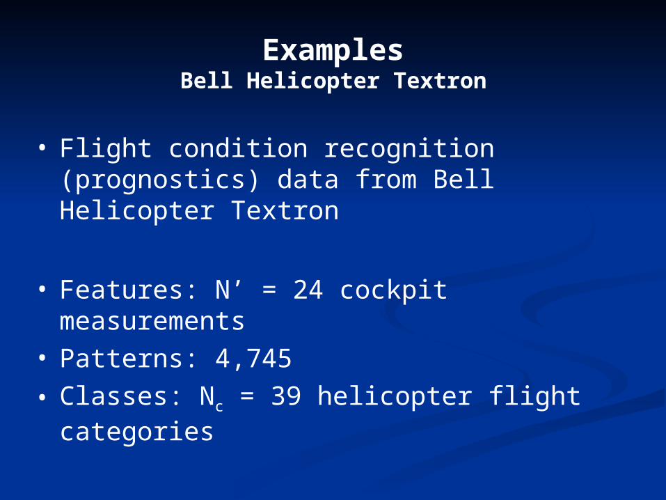
ExamplesBell Helicopter Textron

• Flight condition recognition (prognostics) data from Bell Helicopter Textron

• Features: N’ = 24 cockpit measurements• Patterns: 4,745

• Classes: Nc = 39 helicopter flight categories

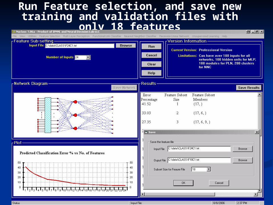
Run Feature selection, and save new training and validation files with only 18 features

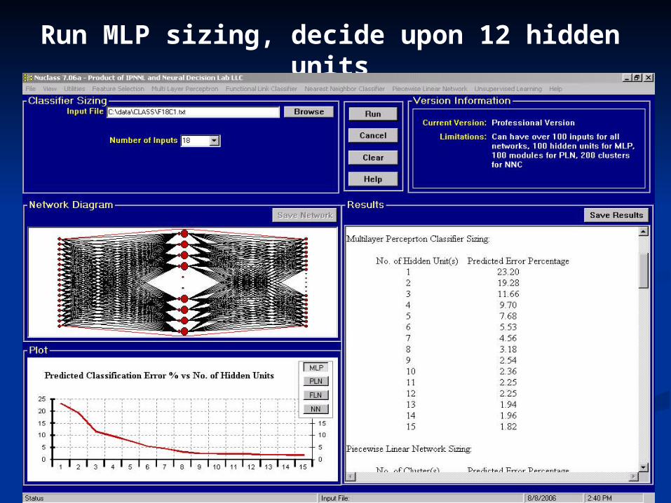
Run MLP sizing, decide upon 12 hidden units

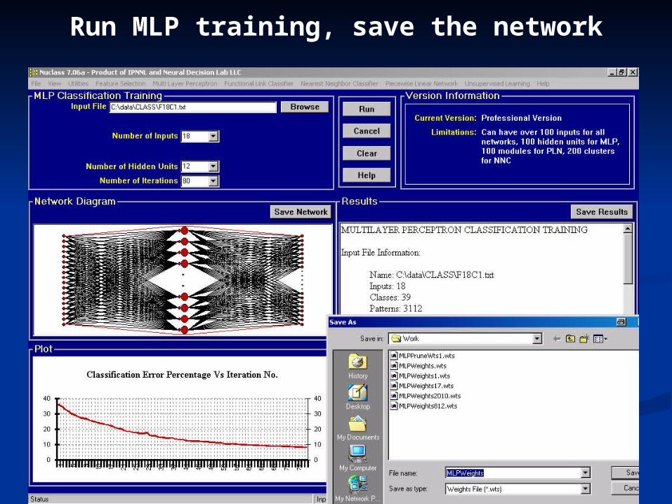
Run MLP training, save the network

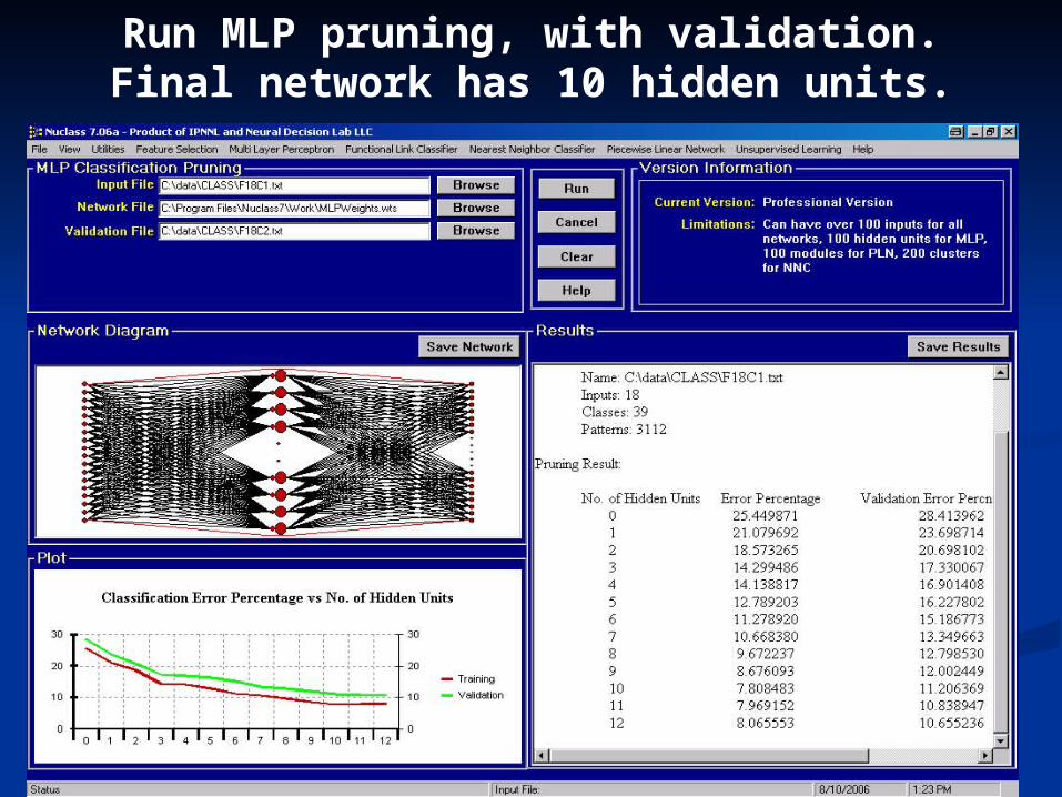
Run MLP pruning, with validation. Final network has 10 hidden units.

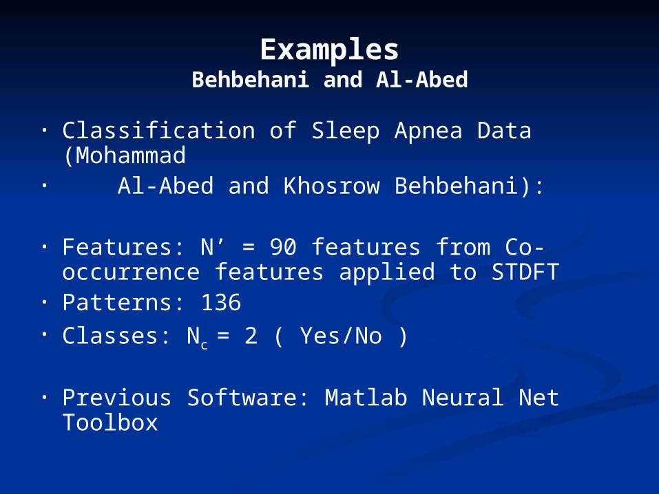
• Classification of Sleep Apnea Data (Mohammad • Al-Abed and Khosrow Behbehani):

• Features: N’ = 90 features from Co-occurrence features applied to STDFT

• Patterns: 136• Classes: Nc = 2 ( Yes/No )

• Previous Software: Matlab Neural Net Toolbox

ExamplesBehbehani and Al-Abed

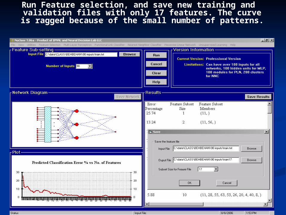
Run Feature selection, and save new training and validation files with only 17 features. The curve is ragged because of the

small number of patterns.

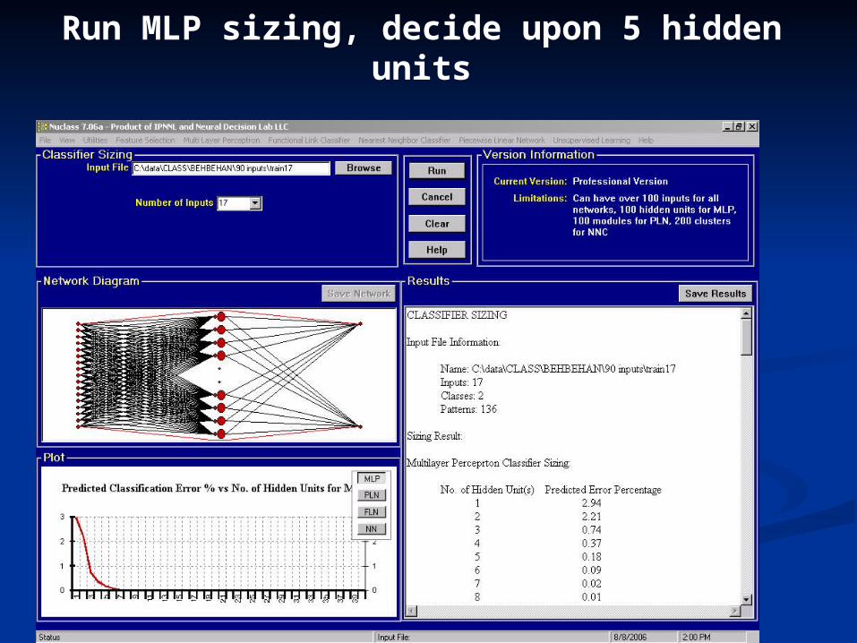
Run MLP sizing, decide upon 5 hidden units

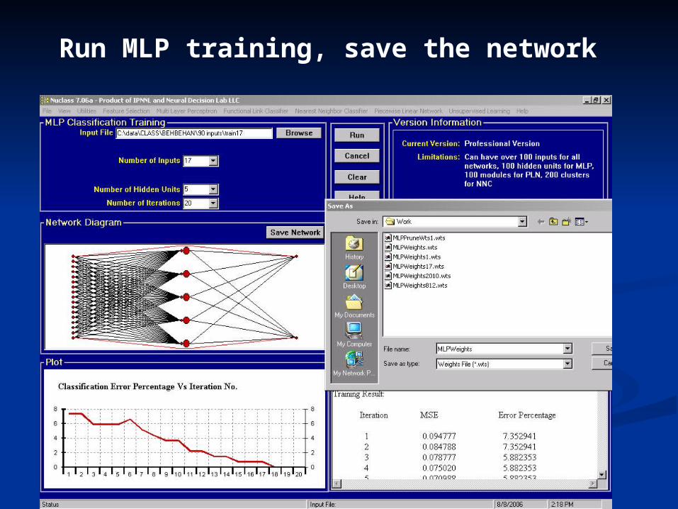
Run MLP training, save the network

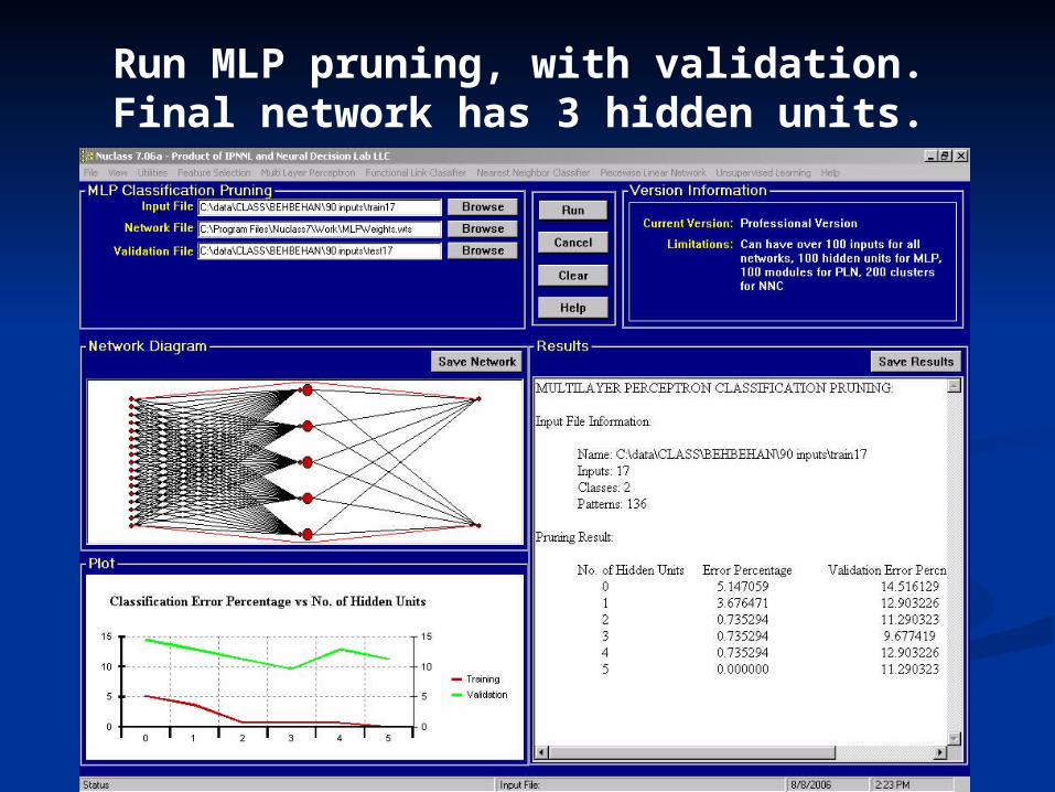
Run MLP pruning, with validation. Final network has 3 hidden units.

Examples- Mattingly and Rasmidatta

• Classification of traveler characteristics d data (Isaradatta Rasmidatta and Steve Mattingly):

• Features: N’ = 22 features• Patterns: 7,325• Classes: Nc = 3 (car, air, bus/train )

• Previous Software: NeuroSolutions by NeuroDimension

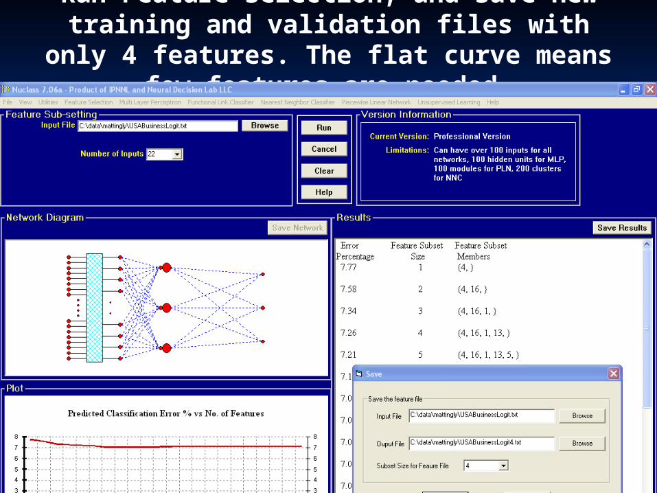
Run Feature selection, and save new training and validation files with only 4 features. The flat curve

means few features are needed.

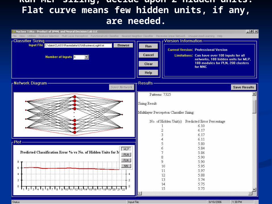
Run MLP sizing, decide upon 2 hidden units. Flat curve means few hidden units, if any, are needed.

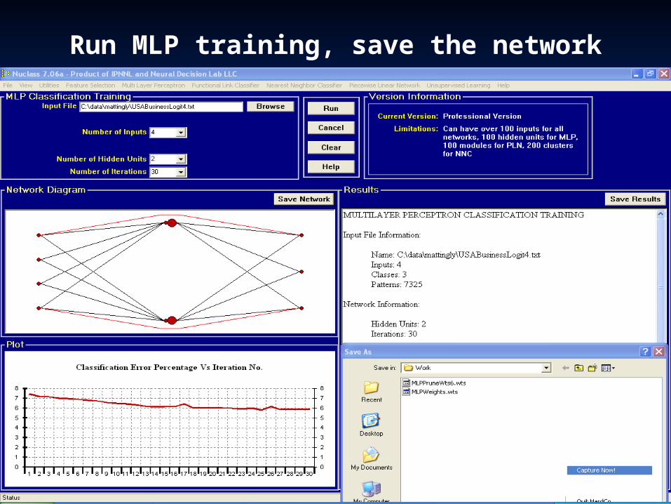
Run MLP training, save the network

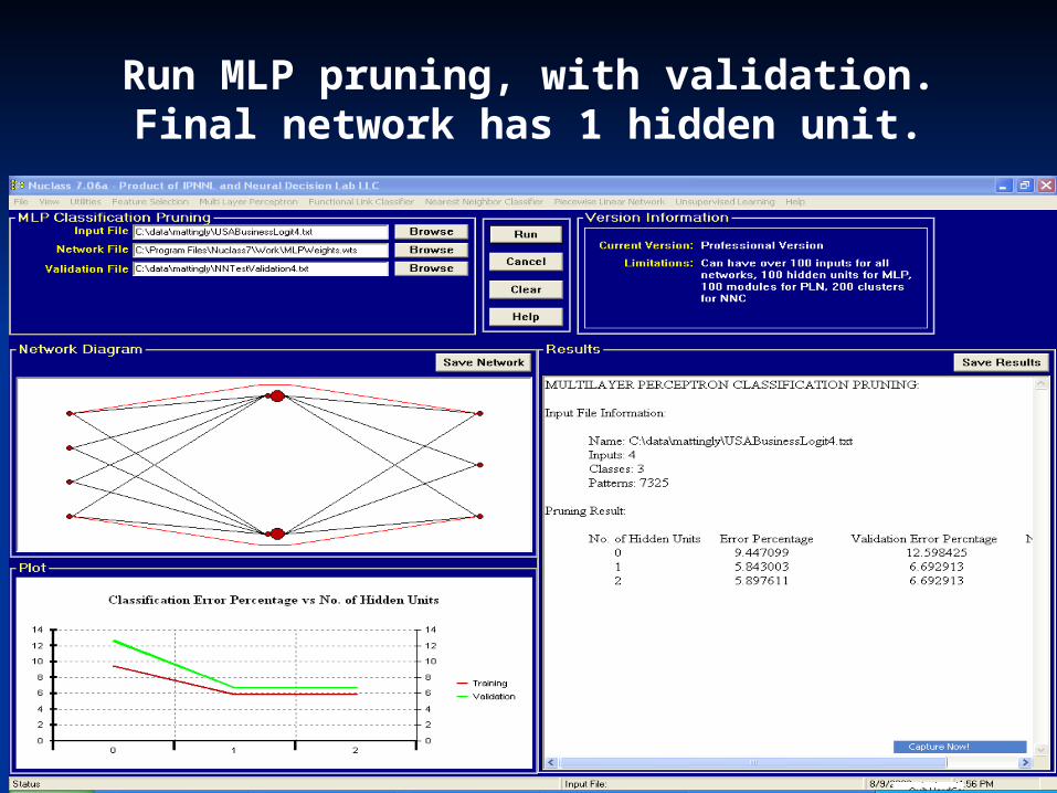
Run MLP pruning, with validation. Final network has 1 hidden unit.

Conclusions • An effective feature selection algorithm has been developed

• Regression-based networks are compatible with CM

• Regression-based training can extend maximal margin concepts to many nonlinear networks

• Several existing and potential blocks in the IPNNL Optimization System have been discussed

• The system has been demonstrated on three pattern recognition applications

• A similar Optimization System is available for approximation/regression applications

ReferencesReferences

[1] K. Fukunaga, Introduction to Statistical Pattern Recognition, 2nd edition, Academic Press, 1990.[2] P. Pudil, J. Novovicova, J. Kittler, " Floating Search Methods in Feature Selection " Pattern Recognition

Letters, vol 15 , pp 1119-1125, 1994 [3] Jiang Li, Michael T. Manry, Pramod Narasimha, and Changhua Yu, “Feature Selection Using a Piecewise

Linear Network”, IEEE Trans. on Neural Networks, Vol. 17, no. 5, September 2006, pp. 1101-1115 [4] Vladimir N. Vapnik, Statistical Learning Theory, John Wiley & Sons, 1998. [5] Duda, Hart and Stork, Pattern Classification, 2nd edition, John Wiley and Sons, 2001.[6] Dennis W. Ruck et al., "The Mulitlayer Perceptron as an Approximation to a Bayes Optimal Discriminant

Function," IEEE Trans. on Neural Networks, Vol. 1, No. 4, 1990.[7] Simon Haykin, "Neural Networks: A Comprehensive Foundation“, 2nd edition. [8] R.G. Gore, Jiang Li, Michael T. Manry, Li-Min Liu, Changhua Yu, and John Wei, "Iterative Design of

Neural Network Classifiers through Regression". International Journal on Artificial Intelligence Tools, Vol. 14, Nos. 1&2 (2005) pp. 281-301.

[9] F. J. Maldonado and M.T. Manry, "Optimal Pruning of Feed Forward Neural Networks Using the Schmidt Procedure", Conference Record of the Thirty Sixth Annual Asilomar Conference on Signals, Systems, and Computers., November 2002, pp. 1024-1028.

[10] P. L. Narasimha, W.H. Delashmit, M.T. Manry, Jiang Li, and F. Maldonado, “An Integrated Growing-Pruning Method for Feedforward Network Training,” NeuroComputing, vol. 71, Spring 2008, pp. 2831-2847.