UCRL-CONF-215410

Optimizing LaboratoryExperiments for DynamicAstrophysical Phenomena

D.D. Ryutov, B.A. Remington

September 15, 2005

6th International Conference on Superstrong Fields in PlasmasVarenna, ItalySeptember 19, 2005 through September 23, 2005

Disclaimer

This document was prepared as an account of work sponsored by an agency of the United States Government. Neither the United States Government nor the University of California nor any of their employees, makes any warranty, express or implied, or assumes any legal liability or responsibility for the accuracy, completeness, or usefulness of any information, apparatus, product, or process disclosed, or represents that its use would not infringe privately owned rights. Reference herein to any specific commercial product, process, or service by trade name, trademark, manufacturer, or otherwise, does not necessarily constitute or imply its endorsement, recommendation, or favoring by the United States Government or the University of California. The views and opinions of authors expressed herein do not necessarily state or reflect those of the United States Government or the University of California, and shall not be used for advertising or product endorsement purposes.

1

Optimizing Laboratory Experiments for Dynamic Astrophysical Phenomena

D.D. Ryutov, B.A. Remington

Lawrence Livermore National Laboratory, Livermore, CA 94551, USA

Abstract. To make a laboratory experiment an efficient tool for the studying the dynamical astrophysical phenomena, it is desirable to perform them in such a way as to observe the scaling invariance with respect to the astrophysical system under study. Several examples are presented of such scalings in the area of magnetohydrodynamic phenomena, where a number of scaled experiments have been performed. A difficult issue of the effect of fine-scale dissipative structures on the global scale dissipation-free flow is discussed. The second part of the paper is concerned with much less developed area of the scalings relevant to the interaction of an ultra-intense laser pulse with a pre-formed plasma. The use of the symmetry arguments in such experiments is also considered.

1. INTRODUCTION

In laboratory experiments with intense lasers, images are sometimes produced

that are strikingly similar to those published in the astrophysical literature. One can compare, for example, “elephant trunks” of photoevaporated molecular clouds [1] and their laboratory analog obtained in the studies of the ablation front instabilities [2]; deeply non-linear bubble-and-spike structures obtained in numerical simulations of the exploding supernova [3] and the laboratory images of such structures [4]; irregular shape of the supernova-driven blast waves [5] and shadowgrams of the laser-driven, irregular blast waves in the laboratory [6]; curved jets generated by young stellar objects (e.g., [7]) and similar jets generated with miniature Z-pinches [8]. Numerous other examples can be found in review papers [9-11].

However impressive, this “likeness” does not necessarily mean that the structures produced in the laboratory can help in unfolding the mysteries of their astrophysical counterparts. In order to make a more meaningful connection, it is desirable to demonstrate that there is a scaling invariance of the basic equations describing the astrophysical system and its laboratory counterpart. This is a difficult task and only in a few cases, mostly in the realm of ideal magnetohydrodynamics (MHD), have such transformations been found (and successfully used).

After a brief general outline of the issues of MHD similarity relevant to astrophysics (Sec. 2.1), we discuss a problem associated with possible role of small-scale dissipative vortices in the systems which are robustly “ideal” on the global scale (Sec. 2.2). In Sec. 2.3, we consider the possibility of solving this problem by means of an experiment based on a so-called “perfect similarity” [12]. If properly designed, such an experiment can considerably advance our understanding of strongly turbulent flows, both in the laboratory and astrophysics. In Sec. 3, we switch to the issues associated with the interaction of ultra-intense laser radiation with a plasma. We find some symmetry properties that determine the structure of the quasi-static magnetic field that is often generated in such setting (Sec. 3.1), and discuss several scalings for the case of a collisionless plasma (secs. 3.2-3.4). Finally, Sec. 4 contains a brief summary.

2

2. SIMILARITIES IN THE IDEAL MHD

2.1 The Euler similarity Because of very large spatial scales of the astrophysical objects, the dimensionless parameters that determine the role of dissipation (the Reynolds number, the Peclet number, and the magnetic Reynolds number) are very large, signifying that the dissipation (viscous, thermal, and Ohmic, respectively) is negligible at the global scale. We also assume that the matter is polytropic, i.e., the internal energy is proportional to the pressure. Under such circumstances, one can describe the medium by the Euler equations:

!

"#

"t+$ % #v = 0 , (1)

!

"#v

#t+ v $ %v

&

' (

)

* + = ,%p +

(% - B) - B

4., (2)

!

"p

"t+ #p$ % v = 0, (3)

!

"B

"t=# $ [v $ B], (4)

where we use CGS system of units and the notation is standard. If the evolution of the system leads to formation of shocks, they can be naturally folded into the Euler description by introducing familiar shock boundary conditions (e.g., [13]).

In the laboratory experiment, the experimental package made of several layers of different materials is driven by the ablation pressure applied at one side of the package. The shock is generated, propagates into the package, and sets the medium in the motion that is supposed to imitate the motion of a real object. Typically, solid materials (metals, plastics) are used to make a package. At the solid-state density, mean free path in a plasma formed after passage of the shock, is very small compared to the thickness of every layer of the package, and ideal hydrodynamics holds to a large margin. Therefore, there is a good reason to believe that both systems can indeed be described by the Euler equations.

It is desirable that the medium used in the laboratory experiment had equations of state deviating not too strongly from that for the polytropic gas; however, even if some deviations are present, one should not expect the appearance of any dramatic differences, because the Euler equations are structurally stable with respect to the moderate variations of the equation of state.

Equations (1-4) possess the following similarity (which was called “Euler similarity” in Refs. [14, 15]): Assume that the initial distributions of density, pressure, velocity, and magnetic field in two systems are geometrically similar, i.e., they can be described by the functions ρ|t=0= ρ*f(r/L*), p|t=0=p*g(r/L*), v|t=0=v*h(r/L*), B|t=0 =B*k(r/L*), with the functions f, g, h, k being the same between the two systems. Parameters marked by the asterisk are scaling factors which can be different between the two systems. It was shown in Refs.[14, 15] that the two systems evolve in the identical way (up to the corresponding scaling factors, i.e., the choice of the particular values of L*, ρ*, p*, v*, and B*) if two number,

3

!

Eu " v * #* / p* (5) (which was called the Euler number in Ref. [14]) and

!

" #8$p*

B*2

(6)

are the same for the two systems. This is a very broad similarity, because it imposes only two constraints on five scaling factors characterizing the initial state. Importantly, the Euler similarity covers the possible presence of shocks. It can also be generalized to the case of ideal magnetohydrodynamics [15].

In the laboratory experiment, by changing the shape of the laser pulse, the experimentalist has certain degree of control over the time dependence of the ablation pressure. By changing it, he/she can change the temporal evolution of the shock wave strength and the density and pressure distribution in the package. One can also vary the materials constituting the package and thickness of the layers. This allows creating a broad range of dynamical settings suitable for modeling various astrophysical problems.

2.2. Possible role of viscosity at large Reynolds numbers

To be specific, we discuss these effects in conjunction with a particular problem, that of developing deeply non-linear structures in the Rayleigh-Taylor instability. At the early stage of the instability, the ideal hydrodynamics certainly works (provided the Reynolds number for the global scale is large enough, as it usually is). The problem arises if the shear-flow turbulence develops and generates small-scale vortices reaching the dissipative scale Δdiss<<<L*. These vortices, of course, do not appear instantaneously: it takes several turn-over times at the global scale (several L*/v*) for them to appear. In other words, the Euler similarity (with dissipative terms neglected) will correctly describe an early stage of the instability, until small-scale vortices are formed. [We are referring to smooth transitions between various materials, with the transition scale-length of order L*; if one deals with a sharp (zero-scale) transition, small-scale perturbations may appear early in the pulse]. During this early stage there is no need to make any assumptions about the turbulent viscosity, introduce Reynolds stresses, and other approximate ways of description: the Euler equations correctly describe this stage, including formation of smaller-scale vortices. In a number of cases, including the SN explosion and its laboratory simulation, this means that essentially the whole physical process is correctly described by Euler equations, with viscosity neglected: within the time ~ several L*/v* the system already reaches a very different state of a strong mix. It is interesting however to assess an issue of what would happen later in time, were there a need to study this later evolution. The question is to what extent will behavior of the two systems be similar at the larger scales if Reynolds numbers, though very large, are different in the two systems (meaning that relative values of the dissipative scales are different). One can argue that the differences on the global scale will be not very large; they will probably appear in the terms of order of lnRe, or in terms that depend on Re even weaker. The reason for this hypothesis is that in a number of relevant problems exhaustively studied experimentally the situation is just this. Examples include the turbulent pipe flow (e.g., [13], and a turbulent flow past an isolated body at high Reynolds number.

4

A possible approach to answering this question might be studying the evolution of two systems which are scalable to each other in the ideal hydrodynamics but would have different Reynolds numbers. Then, the differences in their behavior (other than associated with the scaling transformations) would be a measure of the dissipative effects. However, applying the Euler scaling for isolating subtle dissipative effects is difficult, because the equations of state (EOS) in the regimes typical for high-energy density (HED) hydrodynamic experiments are usually known relatively poorly. Also poorly known are dissipative coefficients, like kinematic viscosity and thermal diffusivity. Therefore, a difference in the behavior of the two systems, if present, could be attributed also to the uncertainties caused by a poor knowledge of EOS and dissipative coefficients, and the main question would remain unanswered.

It has recently been pointed out [12] that there is a very simple similarity, called “perfect similarity” in [12], that can in principle be used for answering this intriguing question. In our present paper, after a brief description of the “perfect similarity” we consider energy requirements for HED experiments where this scaling could be used, and possible impact of such factors as heat loss, irreproducibility of experimental data, and molecular mix

2.3. Perfect similarity

Consider a non-dissipative MHD, without making any assumptions with regard to the equation of state, and allowing for a possibility of spatial variation of the chemical composition. In such a case, instead of Eq.(3), one has to use a general energy conservation law for a dissipation-free medium:

!

"#

"t+ v $ %# = & # + p( )% $ v (7)

where ε =ε (p,ρ, C) is the internal energy per unit volume. For a polytropic gas, with ε=const⋅p, one recovers Eq. (3), with γ =1+1/const. The parameter C in Eq. (7) is used to characterize a fluid with a varying composition. If one deals with a more than a 2-component fluid, one can introduce several such parameters. As, in the framework of the ideal hydrodynamics, the mutual diffusion of various materials is negligible, one has:

!

"C

"t+ v # $C = 0 . (8)

The similarity simply consists of transforming r and t to

!

" r = Ar; " t = At , (9) where A is a constant scaling factor, and leaving v*, B*, p*, and ρ∗ unchanged. One can easily check that the set of equations (1), (2), (4), (7), and (8) remains invariant under such a transformation. The same can be easily checked for the other equations thereby proving similarity. One can check that the shock boundary conditions are also invariant.

No approximations with regard to equation of state are involved, whence the suggested term “perfect similarity” (PS). The perfect similarity holds for an arbitrary equation of state; for an arbitrary varying composition; and in the presence of shocks. So, all the differences in the behavior of two systems related to each other by this similarity would be a direct measure of the role of non-ideal effects.

5

To be specific, we will refer to a small scale system as an “unprimed” system, and to a large-scale system as a “primed” one. Obviously, the energy required for driving a “primed” experiment is (Cf. Ref. [16]):

!

" W = A3W , (10)

An important merit of the perfect similarity is that it does not change transport coefficients (e.g., shear kinematic viscosity ν) which remain equal at the corresponding points of the initial and primed systems (this is because the viscosity ν is a function of p, ρ, and C, which are equal in the corresponding points of the two systems). Accordingly, the Reynolds number,

!

Re = Lv /" , scales as

!

R " e = ARe . The same is true for the Peclet number,

!

Pe = Lv /" , the Peclet mass number,

!

Pem

= Lv /D,and the magnetic Reynolds number,

!

ReM

= Lv /DM

(where χ, D, and DM are thermal diffusivity, inter-spieces diffusion coefficient, and magnetic diffusivity):

!

R " e = ARe; P " e = APe; P " e m

= APem; R " e

m= ARe

m (11)

As we are dealing with the systems which are non-steady-state and non-uniform, the aforementioned dimensionless parameters are introduced in some “characteristic” point both in space and time. The allowance for the spatial variation of transport coefficients (including sharp jumps at interfaces, if the interfaces are present) is a strong point of the “perfect similarity” approach. One can be certain that in two systems related to each other by the PS transformation the transport coefficients in the corresponding points will be identical, and any difference in the global evolution would be related only to the effect of small-scale motions.

As an illustration, we discuss the possibility of applying the perfect similarity approach to an experiment on the development of the Richtmyer-Meshkov (RM) and Rayleygh-Taylor (RT) instability of the bump on the interface of two different materials, as shown on Fig. 1.

A deeply nonlinear evolution of pre-imposed perturbation on the interface between the plastic and CH foam was studied in the experiments [17, 18]. These experiments were carried out with the Omega laser, with the use of ten beams and the total laser energy delivered to the target ~ 5 kJ. The characteristic diameter of the package d was ~ 800 µm. It was enclosed in a tube (in most cases, Beryllium) to delay the propagation of a shock around the sides of the target. The characteristic wavelength λ of perturbations was ~ 50-70 µm. An accuracy of measuring geometrical dimensions of the Rayleigh-Taylor structures was in the range of 5% -10%. As reduction of the drive energy is of much importance for the perfect similarity approach (see Eq. (10)), it is beneficial to study the evolution of a single axisymmetric bump (dimple), as shown on Fig. 1, not a multi-wave perturbation as in Refs. [17, 18]. Taking the radius of the dimple r0 to be 70 µm, and leaving a 70 µm gap between the edge of the dimple and the beryllium tube, one finds that the inner diameter of the tube can be made equal to d~280 µm. This reduction of the tube diameter from ~ 800 mm, would allow one to reduce the required drive energy by a factor of ~ 8, i.e., to approximately 0.6 kJ. The Reynolds number Re in experiments [17, 18] was of order of 105. It will be approximately the same in the experiment with the axisymmetric dimple mentioned above. For sometimes assumed logarithmic dependence of the global scale motion on the Reynolds number (e.g., [13]), changing the latter from 105 to 2⋅105 (i.e., changing the energy form 0.6 to 5 kJ) would mean a change of order of ~5% in the global- scale

6

motion. This may already be distinguishable. A power-law dependence of the global-scale dynamics on the Reynolds number would be much easier to find.

In the systems of the type shown on Fig. 1, the shear-flow turbulence is driven by an “external” (in this case, the RT) instability. Such systems are inherently non-steady-state, and the turbulence has to respond to the changing external conditions. Without getting into any details of this complex problem, which is still an area of active research (e.g., [14, 15] ), we just mention that, if the dissipative-scale vortices have not been formed yet, both systems should evolve according to equations of the ideal hydrodynamics. In this case, there will be no difference between the primed and unprimed systems, aside from the difference in scales (see a caveat regarding possible probabilistic effects later in this section). The time required for the vortices at the dissipation scale to develop depends on the Reynolds number. Therefore, if the difference between the outcomes of the two experiments is present, this may mean that one of them has reached the state of developed turbulence, whereas the other has not.

The development of small-scale vortices may depend on whether the transition between two materials is smooth, with a gradual variation of density, or sharp, with a step-wise density variation (see Ref. [3] for more detail). In the latter case, the small-scale perturbations are driven at an early stage directly by the RT instability, whereas at the former case they are not. In astrophysical systems the transition between various layers is typically relatively smooth.

It was tacitly assumed in our analysis that the large-scale motion is perfectly reproducible in both the initial and primed systems, up to possible inaccuracies in the manufacturing the targets. On the other hand, it may happen that the turbulence would have a “bursty” behavior at the relatively large scales, still resolvable in the images of the global flow and covered by the ideal hydrodynamics. As the bursts may have a statistical character, they would lead to shot-to-shot irreproducibility of the images and make a direct comparison between the primed and unprimed systems impossible.

The presence of bursts can be checked in the experiments with the unprimed (small-scale) system. Taking several shots with the identical initial conditions and comparing the images of the flow at the same instants of time, one would be able to detect the bursty behavior. If these bursts are present and appear in a statistical fashion (which may or may not be the case), one would have to resort to a statistical approach, by making a several “identical” shots in both primed and unprimed systems, averaging the images, and comparing the results for the averaged images. This would, of course, be more costly than in the case where the global flow is deterministic.

5. SYMMETRIES AND SIMILARITIES FOR ULTRA-INTENSE

LASERS

5.1 Discrete symmetries

The development of ultra-intense lasers started with the pioneering paper [19] has opened up new possibilitites in studying astrophysics-relevant phenomena in the laboratory (see, e.g., Refs. [20] and [21]). Generally speaking, effects involved require a kinetic description of the plasma particles, and one cannot use the hydrodynamic scalings discussed in the previous sections. We are not aware of any experiments where a scaled

7

imitation of a particular astrophysical dynamic event would have been studied with ultra-intense lasers. So, we discuss here just some general symmetries and scaling relations which may later be applied for such a purpose. These relations are of some value of their own, without any astrophysical connections, as they provide additional tools for the analysis of experimental results.

In this section we consider the pulses with a duration of at least several wave periods (Fig. 2). It turns out that, in such a case, some general conclusions regarding the distribution of quasistatic currents (and magnetic fields) generated by the pulse (e.g., [22]) can be made based on the symmetry arguments. We do not make any assumptions regarding the quiver energy which can be both non-relativistic and relativistic. We use a Cartesian coordinate system with the axis z in the direction normal to the plasma surface; we assume that the incident radiation is directed along z, and the initial plasma parameters do not depend on x and y.

Consider first the structure of quasi-static currents in the case where the incident wave is linearly polarized, with the electric field vector oriented along the x axis. We assume also that the intensity distribution is symmetric with respect to the xz plane, and with respect to the yz-plane (e.g., the focal spot is circular, Fig. 3). We first discuss the symmetries of the x and y components of the current. As the system has two symmetry planes (xz and xy), the current normal to these planes must vanish (there is no preferential direction). Accordingly, the current pattern will look as shown in Fig. 3a. The shape of the streamlines is identical in all four quadrants, whereas mutual directions of the currents are shown by arrows. In principle, finer structures (but possessing the same symmetry) can be also present.

The direction of the z component of the magnetic field generated by these currents is also shown in this figure. These predictions are up to the change of the sign of the currents (and the magnetic field), in all four quadrants simultaneously: to predict the direction, the symmetry arguments alone are insufficient, one has to analyze the details of the laser-plasma interaction (which is not the subject of this paper).

Allowed by the symmetries, is also the z component of the quasi-static current. This current, of course, flows in the positive direction of z in some areas and in the negative direction of z in other areas, with the closure provided by the xy components. Thereby, the presence of the magnetic field of the type shown in Fig. 3b is allowed. The sign of this field, again, cannot be predicted based solely on the symmetry arguments. A very different pattern of the currents would emerge in the case where the incident radiation is circularly polarized, with the focal spot being circular, as before. In this case, the symmetry of the system does not allow a formation of the pattern shown in Fig.3a. The magnetic field now must be axisymmetric. Therefore, the toroidal (azimuthal) component of the magnetic field does not depend on the azimuth. The poloial component is also allowed, generated by the azimuthal current. The field directions cannot be predicted based solely on the symmetry arguments. Note that the condition that the pulse contains many periods of the light wave is important in our discussion. If the pulse is, say, only 1 period long, then the memory of the direction of the fields during the first half-cycle would remain, making the “up” and “down” (as well as “left” and “right”) directions not identical. The circular polarization for a very short pulse also becomes an ill-defined quantity.

8

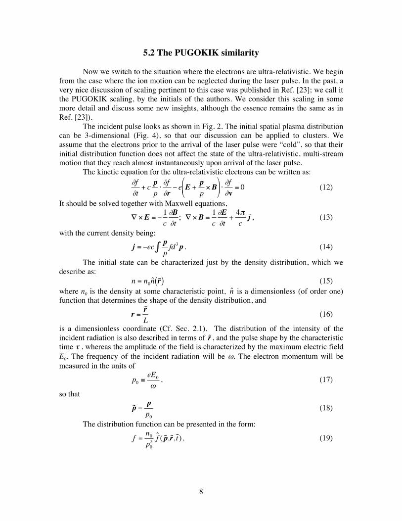
5.2 The PUGOKIK similarity Now we switch to the situation where the electrons are ultra-relativistic. We begin from the case where the ion motion can be neglected during the laser pulse. In the past, a very nice discussion of scaling pertinent to this case was published in Ref. [23]; we call it the PUGOKIK scaling, by the initials of the authors. We consider this scaling in some more detail and discuss some new insights, although the essence remains the same as in Ref. [23]). The incident pulse looks as shown in Fig. 2. The initial spatial plasma distribution can be 3-dimensional (Fig. 4), so that our discussion can be applied to clusters. We assume that the electrons prior to the arrival of the laser pulse were “cold”, so that their initial distribution function does not affect the state of the ultra-relativistic, multi-stream motion that they reach almost instantaneously upon arrival of the laser pulse.

The kinetic equation for the ultra-relativistic electrons can be written as:

!

"f

"t+ cp

p#"f

"r$ e E +

p

p% B

&

' (

)

* + #"f

"v= 0 (12)

It should be solved together with Maxwell equations,

!

" # E = $1

c

%B

%t; " # B =

1

c

%E

%t+4&

cj , (13)

with the current density being:

!

j = "ecp

p# fd

3p . (14)

The initial state can be characterized just by the density distribution, which we describe as:

!

n = n0ˆ n ˜ r ( ) (15)

where n0 is the density at some characteristic point,

!

ˆ n is a dimensionless (of order one) function that determines the shape of the density distribution, and

!

r =˜ r

L (16)

is a dimensionless coordinate (Cf. Sec. 2.1). The distribution of the intensity of the incident radiation is also described in terms of

!

˜ r , and the pulse shape by the characteristic time τ , whereas the amplitude of the field is characterized by the maximum electric field E0. The frequency of the incident radiation will be ω. The electron momentum will be measured in the units of

!

p0"eE

0

#, (17)

so that

!

˜ p =p

p0

(18)

The distribution function can be presented in the form:

!

f =n

0

p0

3

ˆ f ( ˜ p , ˜ r , ˜ t ), (19)

9

where F is some dimensionless function of its arguments. Note that in this formulation the electron rest mass m does not enter the problem. It enters only the applicability condition which reads: p0>>mc (20) The electric and magnetic field will be normalized to E0:

!

E = E0

ˆ E ( ˜ r ,t);B = E0

ˆ B (˜ r ,t) (21) If we are going to compare two system where the frequency of the incident light

is different, say, ω and ω’, then, obviously, in order to have a similarity in the behavior of the two systems we have to change the temporal scale of the pulse, and the spatial scale in such a way that the following two dimensionless parameters remain constant:

!

T "#$ = const,R "#L /c = const (22) With these observations made, one can write equations (12), (13) in the

dimensionless form:

!

1

T

"ˆ f

"˜ t +

1

R

˜ p

˜ p #"ˆ f

"r$ e E +

˜ p

˜ p % ˆ B

&

' (

)

* + #"ˆ f

"˜ p = 0 (23)

!

˜ " # ˆ E = $R

T

% ˆ B

%˜ t ; ˜ " # ˆ B =

R

T

% ˆ E

%˜ t $ SR

˜ p

˜ p & Fd

3 ˜ p (24)

where S is one more dimensionless parameter, identical to the one introduced in the PUGOKIK scaling,

!

S =4"ecn

0

#E0

=4"e2cn

0

# 2p0

(25)

It is the ratio of the plasma density to a relativistically-corrected critical density. In order dimensionless equations (23), (24) to be identical in two systems, the following three constraints have to be satisfied:

T=const; R=const; S=const. (26) There are three constraints on five dimensional parameters, ω, L, τ, E0, and n0 thereby allowing for a significant freedom in choosing the parameters of a scaled experiment (two parameters can be chosen arbitrarily). Consider as an example a scaled experiment where the intensity would be 4 times less than in the initial experiment (i.e,, E0 would be 2 times lower), and the frequency would be 2 times higher. Then, the spatial scale would have to be 2 times smaller (including the transverse size of the incident beam), the pulse-width τ would also have to be reduced by a factor of 2, and the density would have to remain unchanged. Other “derived” parameters of the scaled experiment would change as follows: the total energy of the laser pulse (Joules) will be 32 times lower (!), the quasi-static magnetic field would be 2 times lower, the average electron energy would decrease by a factor of 2, and the reflectivity would remain unchanged.

3.3. Very short pulse. For the case where the duration of the electromagnetic pulse τ becomes comparable to the wave period, the pulse can be adequately characterized just by a single parameter of the dimension of time, τ. There is no need to introduce separately the frequency ω. The definition of p0 can now be changed to

!

p0

= eE0" , and the definition of

R to

!

R = L /c" . The parameter S is changed to

!

S = 4"ec#n0/E

0. There are now four

10

parameters characterizing the system, L, τ, E0, and n0. It is easy to see that in this case the similarity holds if the following two constraints are satisfied: R=const and S=const.

3.4 The ion motion

We now include into consideration the ion motion. We assume that the ions are non-relativistic, whereas the electrons are strongly relativistic, so that Eq. (12) remains valid. The incident pulse compises many periods (Fig.2). The ion mass is M, and the ion charge is Ze. The ion continuity and momentum equations read:

!

dvi

dt=Ze

ME +

1

cvi" B

#

$ %

&

' ( , (27)

!

"ni

"t+# $ (n

ivi) = 0. (28)

In the ion momentum equation we retain the magnetic force to account for the possible effect of a quasistatic magnetic field (the effect of the wave magnetic field on the non-relativistic ions is small). The expression for the current density is:

!

j = "ecp

p# fd

3p + Zenivi . (29)

The ion momentum equation suggests that we presented the ion velocity in the form:

!

vi=

ZeE0"

M

ˆ v i(˜ r , ˜ t ) (30)

with

!

ˆ v i being dimensionless. Then, Eq. (16) becomes:

!

"ˆ v i

"˜ t + Q

T

Rˆ v

i# ˜ $ ̂ v

i= ˆ E + Qˆ v

i% ˆ B (31)

where Q is the following dimensionless parameter:

!

Q =ZeE

0"

Mc= T

ZeE0

Mc# (32)

Normalizing the ion density to n0, one obtains from the continuity equation:

!

" ˜ n i

"˜ t +

QT

R˜ # $ ( ˜ n

i

r ˜ v i) = 0. (33)

Finally, the Bio-Savart equation yields:

!

˜ " # ˆ B =R

T

$ ˆ E

$˜ t % SR

˜ p

˜ p & Fd

3˜ p + ZSRQ ˆ n i ˆ v i (34)

One sees that the invariance of the dimensionless equations is maintained if two additional (to Eq. (26)) conditions are satisfied: the ion charge Z does not change between the two systems, and the parameter Q is held constant:

Z=const, Q=const. (35) Therefore, we see that, adding two more input parameters, the ion charge Z and mass M, leads to the emergence of two more constraints. The system, therefore, still remains quite flexible and amenable to scaled modifications.

Consider the following example: the intensity decreased by a factor of 4, whereas the frequency did not change; we see that the ion mass M has to be decreased by a factor of 2 (e.g., one has to switch from deuterium to hydrogen). The density has to be

11

decreased by a factor of 2, and the length-scale should remain constant. The ion energy remains unchanged.

Consider now an example where the ion species remains unchanged, i.e., not only Z but also M are kept constant between the two experiments. Decreasing the frequency by a factor of 2, one has to reduce the intensity by a factor of 4, and increase the length-scale and the pulse-length by a factor of 2. The density and the ion energy stay constant.

6. SUMMARY

A properly designed laboratory experiment can provide a scalable analog to various astrophysical phenomena, especially those that can be described by the ideal MHD equations. Some difficulty may arise if small-scale dissipative vortices have enough time to develop within the global evolution time. It is at present not quite clear what effect such small-scale vortices would have on a global motion (although there are reasons to believe that the effect will be small). Scaled experiments may provide the opportunity to assess this issue directly, by comparing the results of two experiments related to each other by so-called “perfect similarity.” In the area of interaction of ultra-intense laser pulses with matter, the analysis of possible symmetries and scaled transformations is still at an early stage. However, some inherent symmetries and scalings have been already identified. Scaled experiments may play an important role in identifying possible deviations from the model assumptions and reaching a better understanding of the processes involved in generation of relativistic electrons, fast ions, and generation of quasi-static magnetic fields.

ACKNOWLEDGMENT

This work was performed under the auspices of the U.S. Department of Energy by University of California Lawrence Livermore National Laboratory under contract No. W-7405-Eng-48.

REFERENCES 1. J.J. Hester, P.A. Scowen, R. Sankrit, T.R. Lauer, E.A. Ajhar, W.A. Baum, A. Code, D.G. Currie, G.E. Danielson, S.P. Ewald, S.M. Faber, C.J. Grillmair, E.J. Groth, J.A. Holtzman, D.A. Hunter, J. Kristian, R.M. Light, C.R. Lynds, D.G. Monet, E.J. Oneil, E.J. Shaya, K.P. Seidelman, J.A. Westphal, Astronomical Journ. 111 2349 (1996). 2. B.A. Remington, S.V. Weber, S.W. Haan, J.D. Kilkenny, S.G. Glendinning, R.J. Wallace, W.H. Goldstein, B.G. Wilson, J.K. Nash, Phys. Fluids B5 2588 (1993). 3. E.Muller, B. Fryxell, D. Arnett. Astron. Astrophys., 251, 505 (1991).; K. Kifonidis, T. Plewa, H-Th. Janka, E. Müller. Astrophys. J Letters, 531, 123 (2000). 4. A.R. Miles, et al. Phys. Plasmas, 11, 3631 (2004). 5. http://wave.xray.mpe.mpg.de/rosat/calendar/1997/jul 6. J. Grun, J. Stamper, C. Manka, J. Resnick, R. Burris, J. Crawford, B.H. Ripin. Phys. Rev. Lett., 66, 2738 (1991). 7. B. Reipurth, J. Bally. ARA&A, v. 39, p. 403 (2001). 8. S.V. Lebedev, D. Ampleford, A. Ciardi, S.N. Bland, J.P. Chittenden, M.G. haines, A. Frank, E.G. Blackman, A. Cunningham. ApJ, 616, 988 (2004). 9. B.A. Remington, R.P. Drake, H. Takabe, D. Arnett. Science, 284, 1488 (1999). 10. B.A. Remington, R.P. Drake, H. Takabe, D. Arnett. Phys. Plasmas, 7, 1641 (2000). 11. Remington BA. Plasma Physics & Controlled Fusion, 47, A191 (2005).

12

12. D.D. Ryutov, B.A. Remington. Physics of Plasmas, 10, 2629, 2003; Proc. IFSA-2003, ANS Publications, 2004, pp.945-949. 13. L.D. Landau, E.M. Lifshitz. “Fluid Mechanics,” Pergamon, 1987. 14. D.D. Ryutov, R. P. Drake, J. Kane, E. Liang, B. A. Remington, and W.M. Wood-Vasey. Astrophys. J, 518, 821 (1999); D.D. Ryutov, R.P. Drake and B.A. Remington. Astrophys. J. - Supplement, 127, 465 (2000). 15. D.D. Ryutov, B.A. Remington, H.F. Robey, R.P. Drake, Phys. Plasmas, 8, 1804 (2001). 16. M. Murakami, S. Iida. Phys. Plasmas, 9, 2745 (2002). 17. H.F. Robey, J.O. Kane, B.A. Remington, R.P. Drake RP, O.A. Hurricane, H. Louis, R.J. Wallace, J. Knauer, P. Keiter, D. Arnett, D.D. Ryutov, Phys. Plasmas, 8, 2446, (2001); H.F. Robey, Y. Zhou, A.C. Buckingham, P. Keiter, B.A. Remington, R.P.Drake, Phys Plasmas, 10, 614 (2003). 18. A.R. Miles, M.J. Edwards, J.A. Greenough. Physics of Plasmas, 11, 5278 (2004). 19. D. Strickland and G. Morou. Opt. Commun., 56, 219 (1985). 20. E. Liang, K. Nishimura, Li Hui, S.P. Gary. Phys. Rev. Lett., 90, 085001 (2003). 21. S.J. Moon, S.C. Wilks, R.I. Klein, B.A. Remington, D.D. Ryutov, A.J. Mackinnon, P.K. Patel, A.A. Spitkovsky, Astrophys. Space Sci. 298, 293-298 (2005). 22. P.A. Norreys, K.M. Krushelnick, M. Zepf. Plasma Phys. Contr. Fusion, 46, B13 (2005). 23. A. Pukhov, S. Gordienko, S. Kiselev, I. Kostyukov. “The bubble regime of laser-plasma acceleration: monoenergetic electrons and the scalability,” Plasma Phys. Contr. Fus., 46, B179 (2004).

13

t

Ex, A.U.

τ

2π/ω

Fig. 2 The shape of the incident laser pulse with a duration τ substantially exceeding the wave period 2π/ω

Fig. 1. Possible experiment on the study of the effect of the Reynolds number on the Rayleigh-Taylor instability: a) General experimental setup, with the experimental package accelerated by the ablation pressure (shown in short arrows); the lightly hatched material is denser then the heavily hatched; initial perturbation shown as a bump in the denser material, will evolve into familiar “mushroom” on the nonlinear stage. The difference between two experiments would be the geometric dimensions and the pulse duration; b) Rough sketch of strongly non-linear Rayleigh-Taylor “bubble” originating from the initial bump in a small-scale experiment (1), in a “perfectly similar” larger-scale experiment in the case of weak Reynolds number effects (2), and in the case of substantial Reynolds number effects (3); the structure (2) is geometrically similar to the structure (1), whereas the structure (3) is expected to be longer in the same instance of time as structure (2). We do not show small-scale vortices excited in the interface zone which can be smeared by them.

14

x

y

j⊥

Bz

x

y

B⊥

a b

Fig. 3 Generation of a quasi-steady magnetic field by a pulse with a linear polarization. The intensity distribution shown by the shades of yellow is axisymmetric. The panel (a) depicts a symmetry of the transverse current pattern; this current generates the magnetic field that can be loosely called “poloidal”. In panel (b) the “toroidal” magnetic field is shown (the streamlines are made deliberately non-axisymmetric, to emphasize that there is no axial symmetry in the vectorial characteristics of the laser light, although the intensity distribution is axisymmetric). The axial current that generates toroidal magnetic field is directed away from the viewer near the origin and towards the viewer at the periphery, so that the net quasistatic axial current is zero.

L

Fig. 4 Interaction of a laser beam with an arbitrary oriented non-spherically-symmetric cluster of a characteristic size L.