Embed Size (px)
Citation preview

Optimizing Graph Algorithms for Improved Cache
Performance
Aya Mire & Amir Nahir
Based on: Optimizing Graph Algorithms for Improved Cache Performance – Joon-Sang Park,
Michael Penner, Viktor K Prasanna
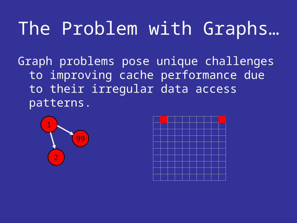
The Problem with Graphs…
Graph problems pose unique challenges to improving cache performance due to their irregular data access patterns.
1
2
99

Agenda
• A recursive implementation of the Floyd-Warshall Algorithm.
• A tiled implementation of the Floyd-Warshall Algorithm.
• Efficient data structures for general graph problem.
• Optimizations for the maximum matching algorithm.
Analysis model
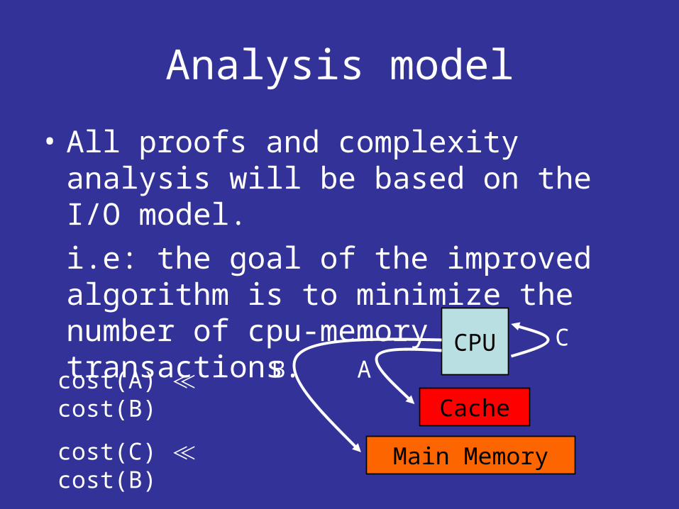
• All proofs and complexity analysis will be based on the I/O model.i.e: the goal of the improved algorithm is to minimize the number of cpu-memory transactions.
CPU
Cache
Main Memory
ABC
cost(A) ≪ cost(B)
cost(C) ≪ cost(B)
Analysis model
All proofs will assume total control of the cache. i.e if the cache is big enough to hold two data blocks, than the two can be held in the cache without running over each other (no conflict misses)

The Floyd Warshall Algorithm
• An ‘all pairs shortest path’ algorithm.• Works by iteratively calculating Dk,
where Dk is the matrix of all pair shortest paths going through vertices 1, 2, …k.
• Each iteration depends on the result of the previous one.
• Time complexity: Θ(|V|3).
The Floyd Warshall Algorithm
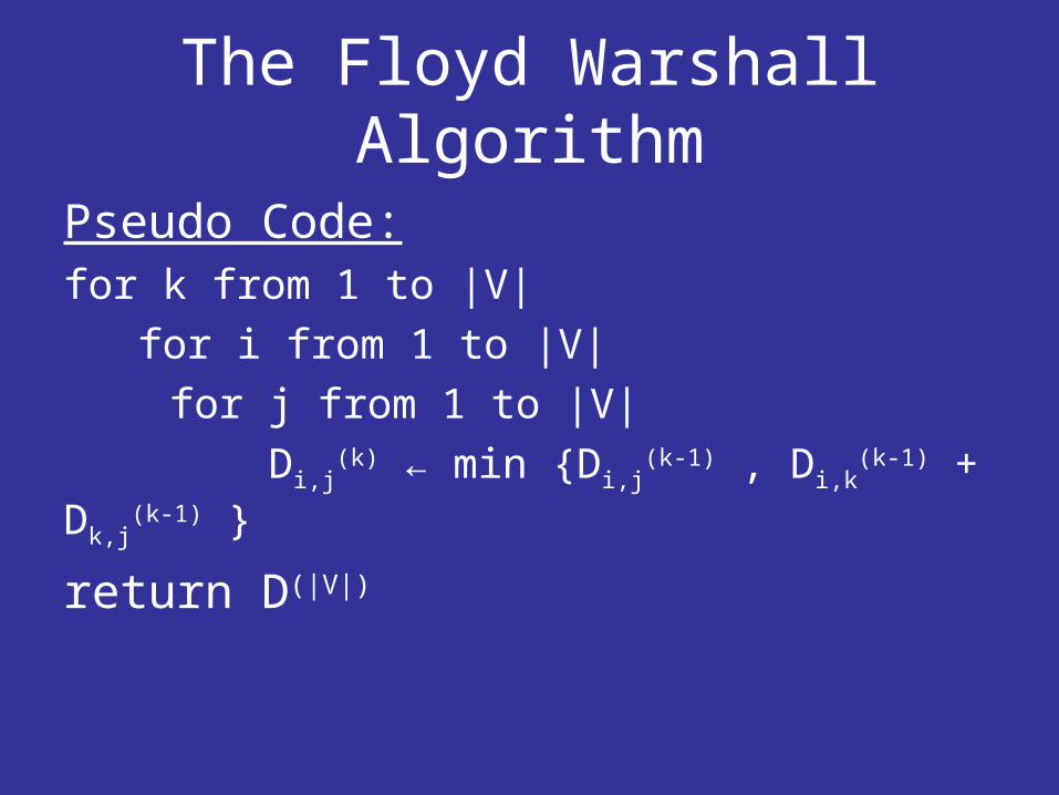
Pseudo Code:for k from 1 to |V| for i from 1 to |V|
for j from 1 to |V| Di,j
(k) ← min Di,j(k-1) , Di,k
(k-1) + Dk,j(k-1)
return D(|V|)

The Floyd Warshall Algorithm
The algorithm accesses the entire matrix in each iteration.
The dependency of the kth iteration on the results of the (k-1)th iteration eliminate the ability to perform data reuse.
Lemma 1
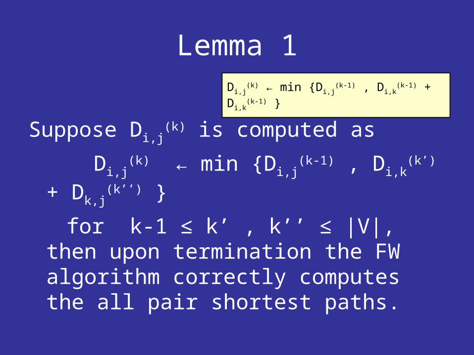
Suppose Di,j(k) is computed as
Di,j(k) ← min Di,j
(k-1) , Di,k(k’) +
Dk,j(k’’)
for k-1 ≤ k’ , k’’ ≤ |V|, then upon termination the FW algorithm correctly computes the all pair shortest paths.
Di,j(k) ← min Di,j
(k-1) , Di,k(k-1) + Di,k
(k-1)
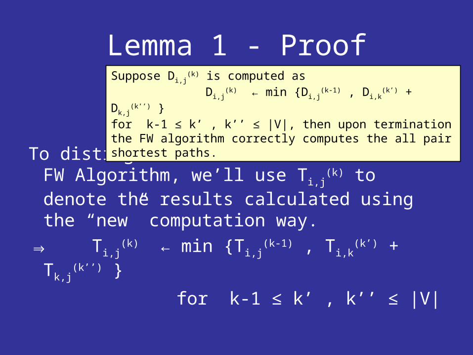
Lemma 1 - Proof
To distinguish between the traditional FW Algorithm, we’ll use Ti,j
(k) to denote the results calculated using the “new” computation way.
⇒ Ti,j(k) ← min Ti,j
(k-1) , Ti,k(k’) + Tk,j
(k’’)
for k-1 ≤ k’ , k’’ ≤ |V|
Suppose Di,j(k) is computed as
Di,j(k) ← min Di,j
(k-1) , Di,k(k’) + Dk,j
(k’’) for k-1 ≤ k’ , k’’ ≤ |V|, then upon termination the FW algorithm correctly computes the all pair shortest paths.

Lemma 1 - Proof
First, we’ll show that for 1 ≤ k ≤ |V| the following inequality holds:
Ti,j(k) ≤ Di,j
(k)
We Prove this by induction.
Base case: by definition we haveTi,j
(0) = Di,j(0)
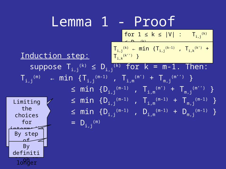
Lemma 1 - Proof
Induction step: suppose Ti,j
(k) ≤ Di,j(k) for k = m-1. Then:
Ti,j(m) ← min Ti,j
(m-1) , Ti,m(m’) + Tm,j
(m’’)
≤ min Di,j(m-1) , Ti,m
(m’) + Tm,j(m’’)
≤ min Di,j(m-1) , Ti,m
(m-1) + Tm,j(m-1)
≤ min Di,j(m-1) , Di,m
(m-1) + Dm,j(m-1)
= Di,j(m)
for 1 ≤ k ≤ |V| : Ti,j(k) ≤ Di,j
(k)
Ti,j(k) ← min Ti,j
(k-1) , Ti,k(k’) + Ti,k
(k’’)
By step of induction
Limiting the choices for
intermediate vertices
makes path same or longer
By step of induction
By definition

Lemma 1 - Proof
On the other hand, since the traditional algorithm computes the shortest paths at termination, and since Ti,j
(|V|) is the length of some path, we have:
Di,j(|V|) ≤ Ti,j
(|V|)
⇒ Di,j(|V|) = Ti,j
(|V|)
for 1 ≤ k ≤ |V| : Ti,j(k) ≤ Di,j
(k)
Suppose Di,j(k) is computed as
Di,j(k) ← min Di,j
(k-1) , Di,k(k’) + Dk,j
(k’’) for k-1 ≤ k’ , k’’ ≤ |V|, then upon termination the FW algorithm correctly computes the all pair shortest paths.
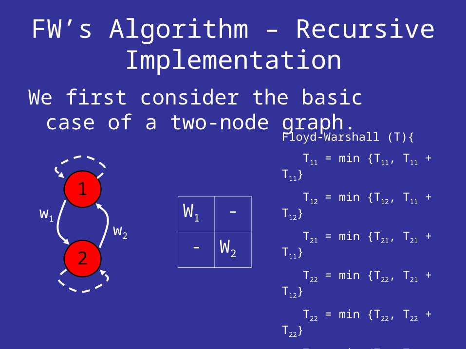
FW’s Algorithm – Recursive Implementation
We first consider the basic case of a two-node graph.
w1
w2
1
2
-W1
W2-
Floyd-Warshall (T)
T11 = min T11, T11 + T11
T12 = min T12, T11 + T12
T21 = min T21, T21 + T11
T22 = min T22, T21 + T12
T22 = min T22, T22 + T22
T21 = min T21, T22 + T21
T12 = min T12, T12 + T22
T11 = min T11, T12 + T21

FW’s Algorithm – Recursive Implementation
The general case
I II
III IV
Floyd-Warshall (T)If (not base case) TI = min TI , TI , TI TII = min TII , TI , TII TIII = min TIII , TIII , TI TIV= min TIV , TIII , TII TIV = min TIV , TIV , TIV TIII = min TIII , TIV , TIII TII = min TII , TII , TIV TI = min TI , TII , TIII else …
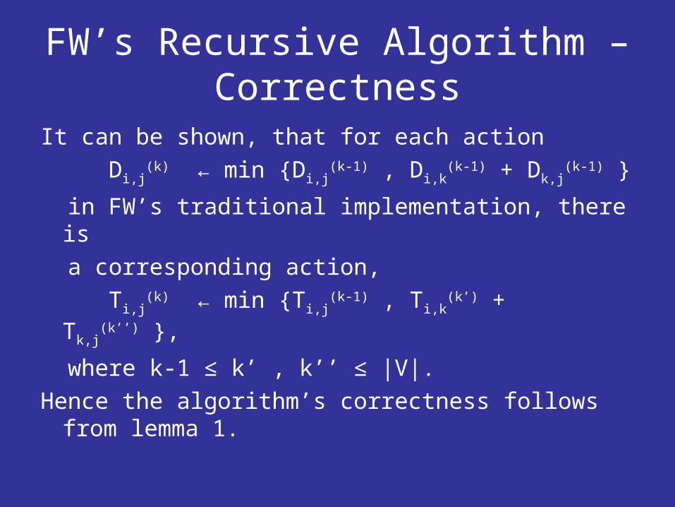
FW’s Recursive Algorithm –Correctness
It can be shown, that for each action Di,j
(k) ← min Di,j(k-1) , Di,k
(k-1) + Dk,j(k-1)
in FW’s traditional implementation, there is a corresponding action, Ti,j
(k) ← min Ti,j(k-1) , Ti,k
(k’) + Tk,j(k’’) ,
where k-1 ≤ k’ , k’’ ≤ |V|.Hence the algorithm’s correctness follows
from lemma 1.
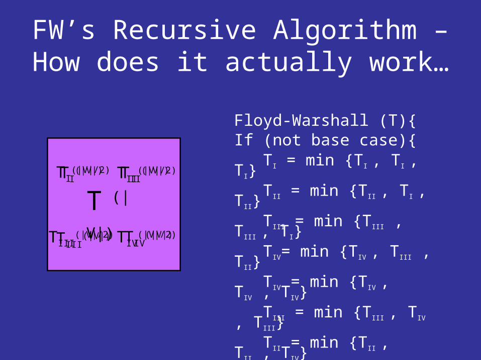
FW’s Recursive Algorithm – How does it actually work…
TI(0) TII
(0)
TIV(0)TIII
(0)
Floyd-Warshall (T)If (not base case) TI = min TI , TI , TI TII = min TII , TI , TII TIII = min TIII , TIII , TI TIV= min TIV , TIII , TII TIV = min TIV , TIV , TIV TIII = min TIII , TIV , TIII TII = min TII , TII , TIV TI = min TI , TII , TIII else …
T (0)T (|V|)
TI(|V|/2) TII
(|V|/2)
TIII(|V|/2) TIV
(|V|/2)TIV(|V|)TIII
(|V|)
TII(|V|)TI
(|V|)
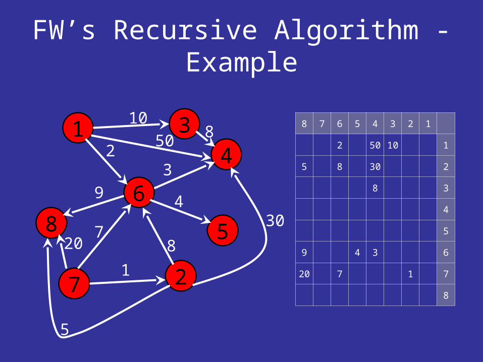
FW’s Recursive Algorithm - Example
1
2
3
68
4
5
7
10
2
30
8
5
8
3
49
1
720
12345678
110502
23085
38
4
5
6349
71720
8
50

FW’s Recursive Algorithm – Example
12345678
1102
23085
38
4
5
6349
717
8
Floyd-Warshall (T)
T11 = min T11, T11 + T11
T12 = min T12, T11 + T12
T21 = min T21, T21 + T11
T22 = min T22, T21 + T12
T22 = min T22, T22 + T22
T21 = min T21, T22 + T21
T12 = min T12, T12 + T22
T11 = min T11, T12 + T21
1850
2016
1-3-4
7-6-8

FW’s Recursive Algorithm – Example
12345678
1102
285
38
4
5
6349
717
8
Floyd-Warshall (T)
T11 = min T11, T11 + T11
T12 = min T12, T11 + T12
T21 = min T21, T21 + T11
T22 = min T22, T21 + T12
T22 = min T22, T22 + T22
T21 = min T21, T22 + T21
T12 = min T12, T12 + T22
T11 = min T11, T12 + T21
18
166
12
6 11
3011
31
7-2-47-6-5
11
7-2-87-6-4
10
1-6-81-6-52-6-51-6-4 52-6-4
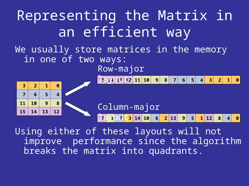
Representing the Matrix in an efficient way
We usually store matrices in the memory in one of two ways:
Using either of these layouts will not improve performance since the algorithm breaks the matrix into quadrants.
0123
4567
891011
12131415
0123456789101112131415
048121591326101437815
Column-major layout:
Row-major layout:

Representing the Matrix in an efficient way
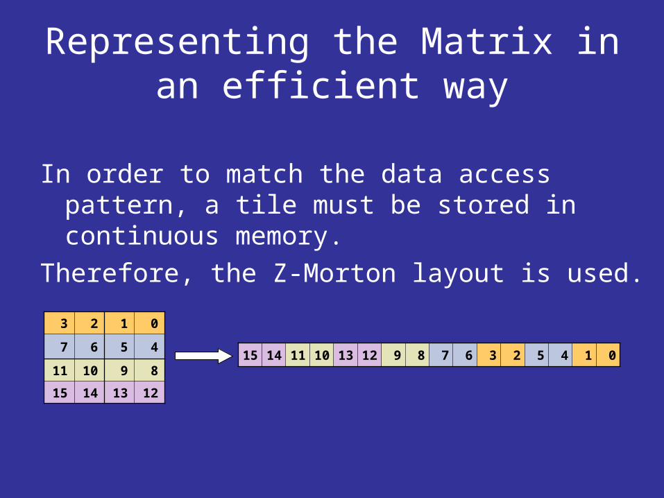
The Z-Morton layout:perform the following operations recursively until the quadrant size is of a single data unit:
divide the matrix into four quadrants.store quadrant I, II, III, IV in the memory.
For example:
0123
4567
891011
12131415
0145236789121310111415

Complexity Analysis
The running time ofthe algorithm is givenby T(|V|) = 8·T(|V|/2) = Θ(|V|3)
Without considering Cache the number of cpu-memory transactionsis exactly as the running time
Floyd-Warshall (T)If (not base case) TI = min TI , TI , TI TII = min TII , TI , TII TIII = min TIII , TIII , TI TIV= min TIV , TIII , TII TIV = min TIV , TIV , TIV TIII = min TIII , TIV , TIII TII = min TII , TII , TIV TI = min TI , TII , TIII else …

Complexity Analysis - Theorem
There exists some B, where B = O(|cache|1/2), such that,
when using the FW-Recursive implementation, with the matrix stored in the Z-Morton layout, the number of cpu-memory transactions will be reduced by a factor of B.
⇒ there will be O(|V|3/B) cpu-memory transactions.

Complexity Analysis
After k recursive calls, the size of a quadrant’s dimension is |V|/2k.
There exists some k, such that B ≜ |V|/2k and3 · B2 ≤ |cache|
Once the above condition is fulfilled, 3 matrices of size B2 can be placed in the cache, and no further cpu-memory transactions are required.
⇒B = O(|cache|1/2)
Floyd-Warshall (T)If (not base case) TI = min TI , TI , TI TII = min TII , TI , TII TIII = min TIII , TIII , TI TIV= min TIV , TIII , TII TIV = min TIV , TIV , TIV TIII = min TIII , TIV , TIII TII = min TII , TII , TIV TI = min TI , TII , TIII else …
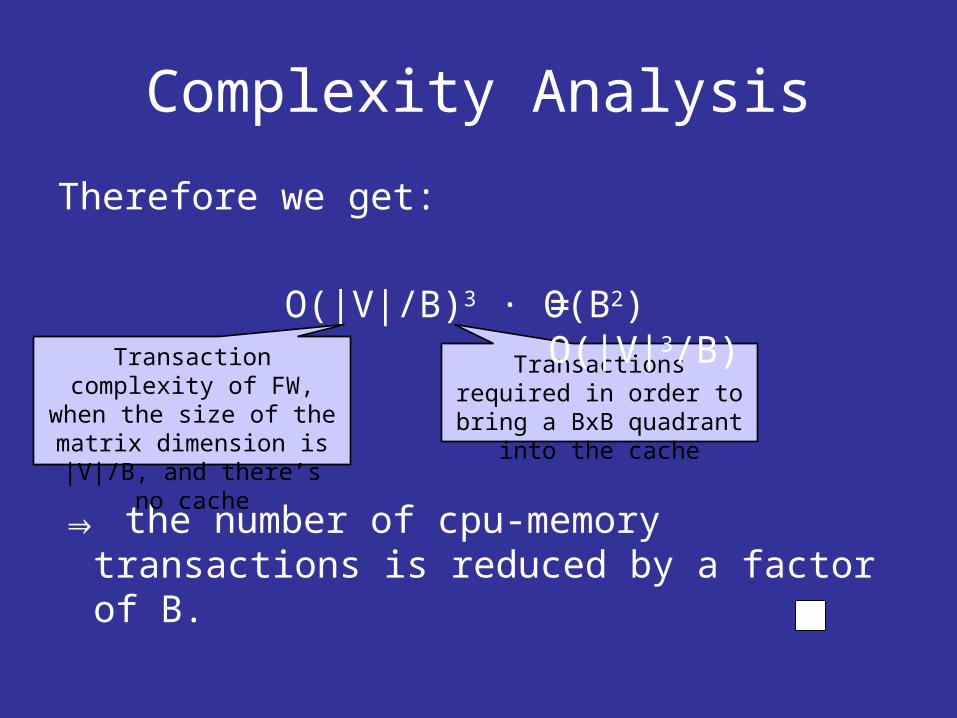
Complexity Analysis
Therefore we get:
O(|V|/B)3 · O(B2)
⇒ the number of cpu-memory transactions is reduced by a factor of B.
Transaction complexity of FW, when the size of the matrix dimension is
|V|/B, and there’s no cache
Transactions required in order to bring a BxB
quadrant into the cache
= O(|V|3/B)
Complexity Analysis – lower bound
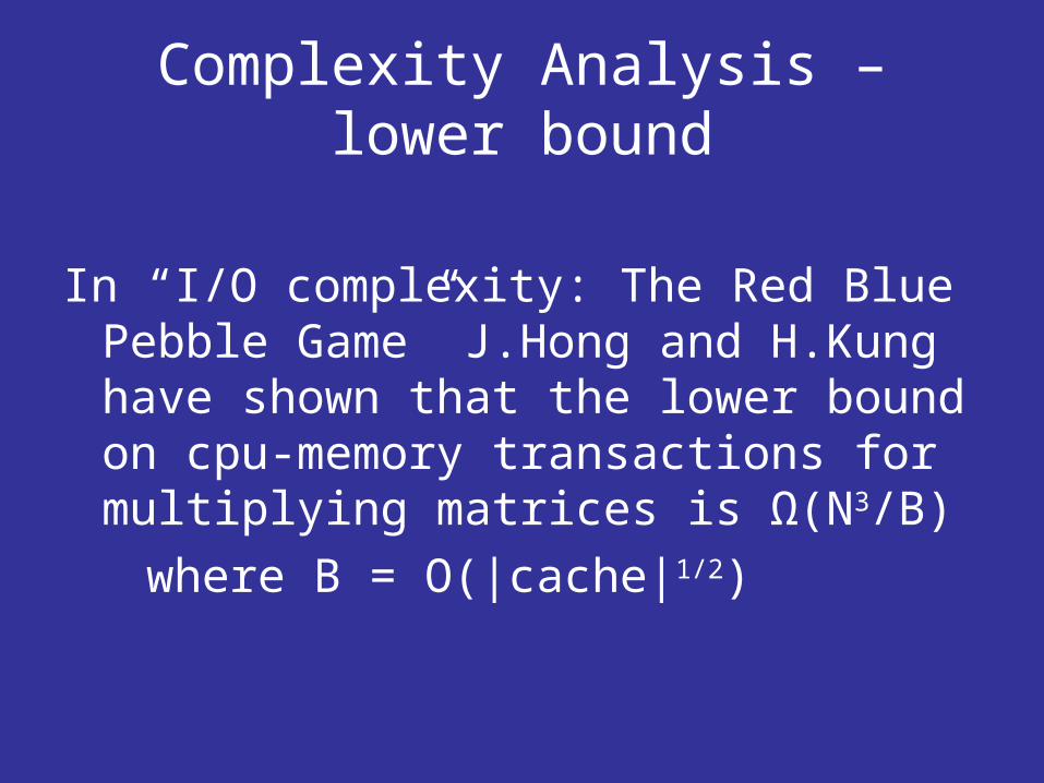
In “I/O complexity: The Red Blue Pebble Game” J.Hong and H.Kung have shown that the lower bound on cpu-memory transactions for multiplying matrices is Ω(N3/B)
where B = O(|cache|1/2)
Complexity Analysis – lower bound – Theorem
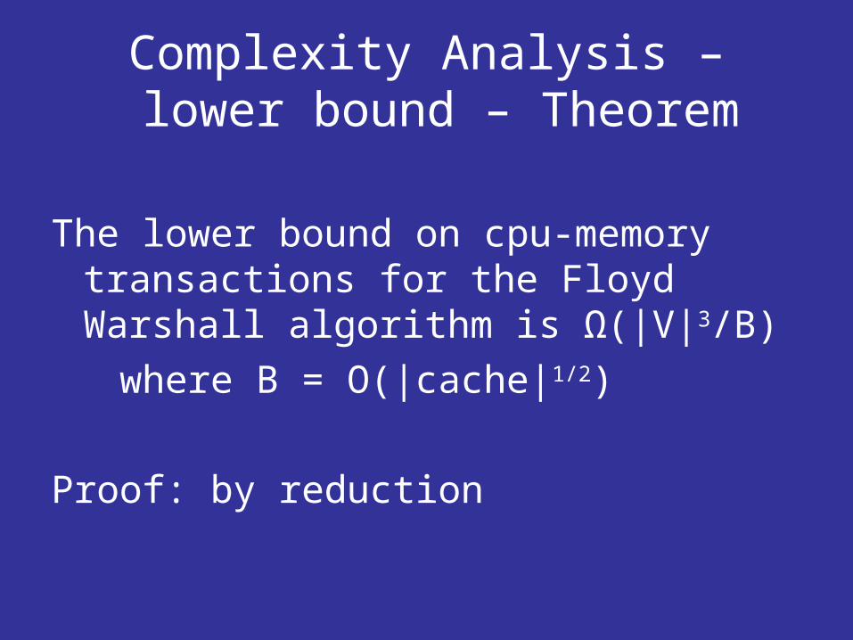
The lower bound on cpu-memory transactions for the Floyd Warshall algorithm is Ω(|V|3/B)
where B = O(|cache|1/2)
Proof: by reduction
Complexity Analysis – lower bound theorem - Proof
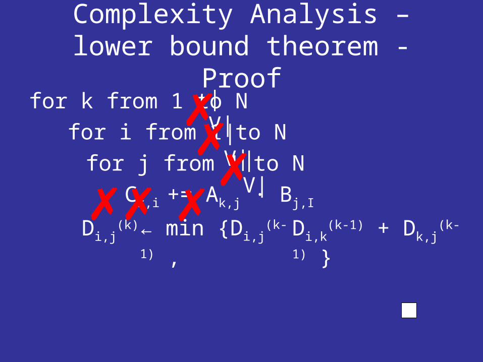
for k from 1 to N for i from 1 to N
for j from 1 to N Ck,i += Ak,j · Bj,I
|V|
|V||V|
Di,j
(k) ← min Di,j(k-
1) ,Di,k
(k-1) + Dk,j(k-1)
Complexity Analysis - Conclusion
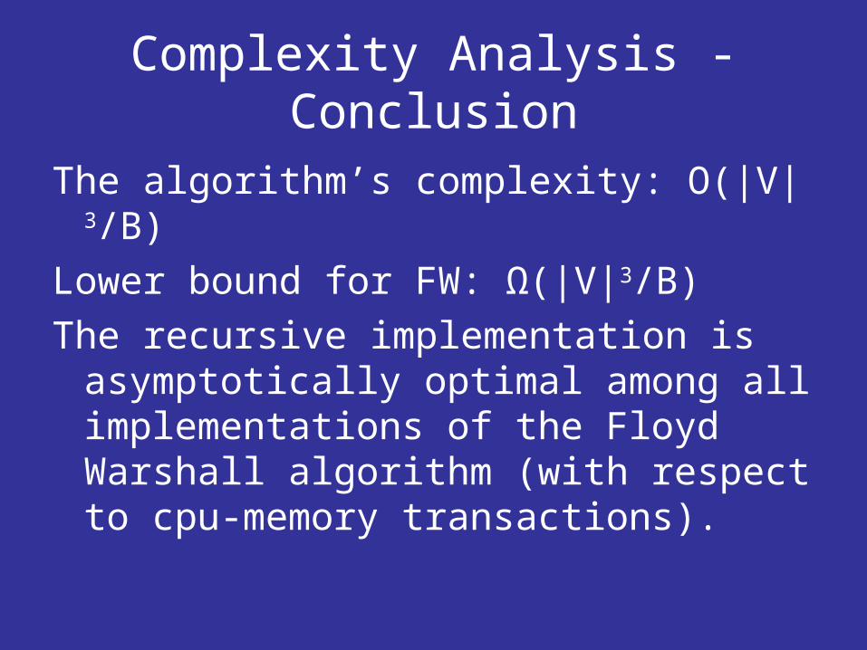
The algorithm’s complexity: O(|V|3/B)Lower bound for FW: Ω(|V|3/B) The recursive implementation is
asymptotically optimal among all implementations of the Floyd Warshall algorithm (with respect to cpu-memory transactions).
FW’s Algorithm – Recursive Implementation - Comments
Note, that the size of the cache is not part of the algorithm’s parameters, neither it is needed in order to store the matrix in the Z-Morton layout.
Therefore:the algorithm is cache- oblivious
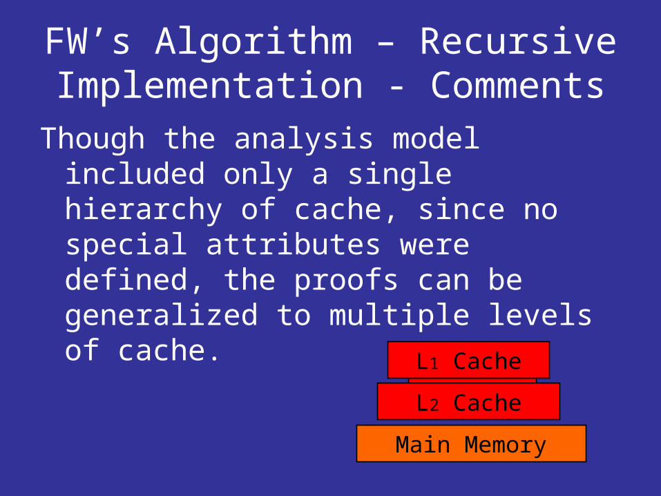
FW’s Algorithm – Recursive Implementation - Comments
Though the analysis model included only a single hierarchy of cache, since no special attributes were defined, the proofs can be generalized to multiple levels of cache.
L0 Cache
Main Memory
L1 Cache
L2 Cache
FW’s Algorithm – Recursive Implementation - Comments
Since cache parameters have been disregarded, the best (and simplest) way to find the optimal size B is by experiment.

FW’s Algorithm – Recursive Implementation - ImprovementThe algorithm can be further improved
by making it cache conscious: performing the recursive calls until the problem size is reduced to B, and solving the B-size problem in the traditional way (saves recursive calls’ overhead)
This modification showed up to 2x improvement of running time on some of the machines.

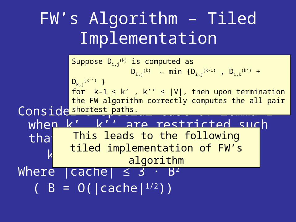
FW’s Algorithm – Tiled Implementation
Consider a special case of lemma 1 when k’, k’’ are restricted such that
k - 1 ≤ k’, k’’ ≤ k - 1 + BWhere |cache| ≤ 3 · B2
( B = O(|cache|1/2))
Suppose Di,j(k) is computed as
Di,j(k) ← min Di,j
(k-1) , Di,k(k’) + Dk,j
(k’’) for k-1 ≤ k’ , k’’ ≤ |V|, then upon termination the FW algorithm correctly computes the all pair shortest paths.
This leads to the following tiled implementation of FW’s algorithm
FW’s Algorithm – Tiled Implementation
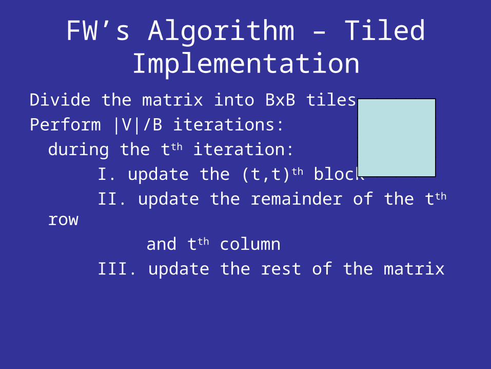
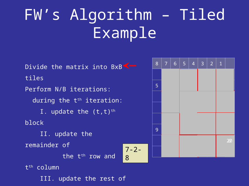
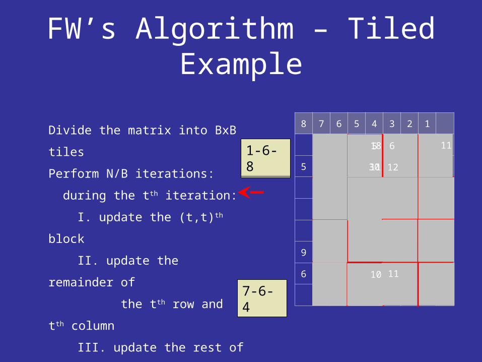
Divide the matrix into BxB tilesPerform |V|/B iterations:
during the tth iteration:I. update the (t,t)th blockII. update the remainder of the tth row
and tth columnIII. update the rest of the matrix

FW’s Algorithm – Tiled Implementation
Each iterationconsists of threephases:
Phase I:performing FW’s algorithms on the (t,t)th tile
(which is self-dependent).
Divide the matrix into BxB tilesPerform N/B iterations: during the tth iteration: I. update the (t,t)th block II. update the remainder of the tth row and tth column III. update the rest of the matrix
FW’s Algorithm – Tiled Implementation
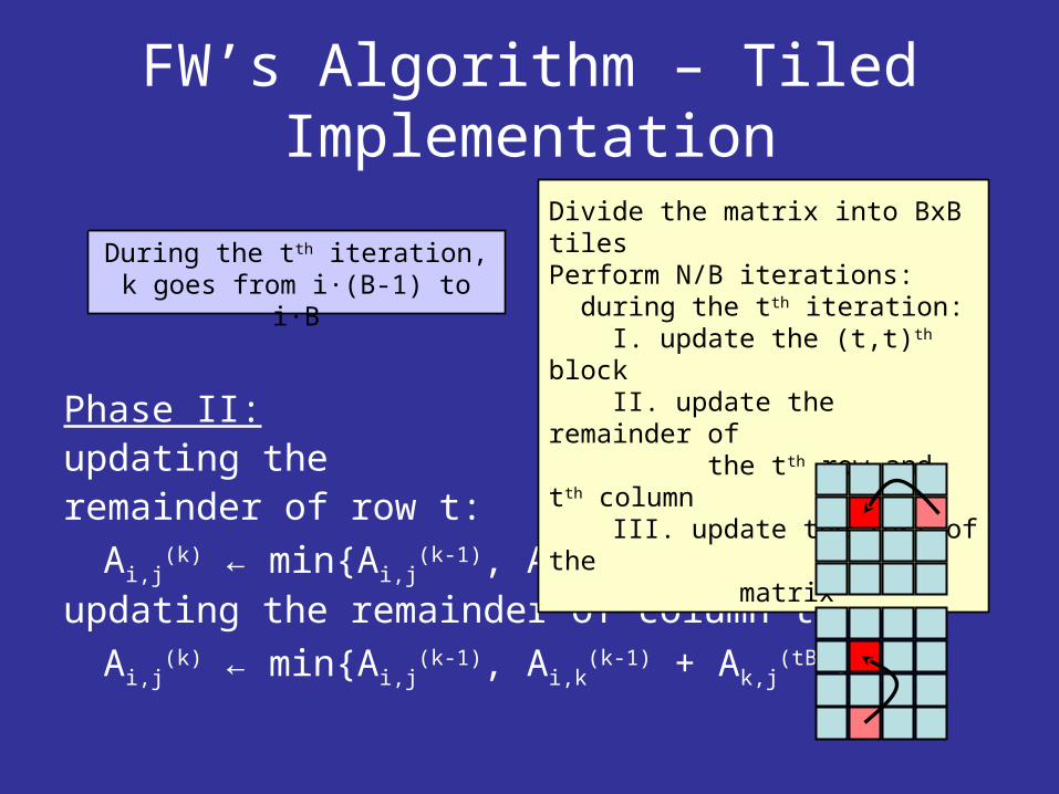
Phase II:updating theremainder of row t:
Ai,j(k) ← minAi,j
(k-1), Ai,k(tB) + Ak,j
(k-1)updating the remainder of column t:
Ai,j(k) ← minAi,j
(k-1), Ai,k(k-1) + Ak,j
(tB)
Divide the matrix into BxB tilesPerform N/B iterations: during the tth iteration: I. update the (t,t)th block II. update the remainder of the tth row and tth column III. update the rest of the matrix
During the tth iteration, k goes from i·(B-1) to i·B
FW’s Algorithm – Tiled Implementation
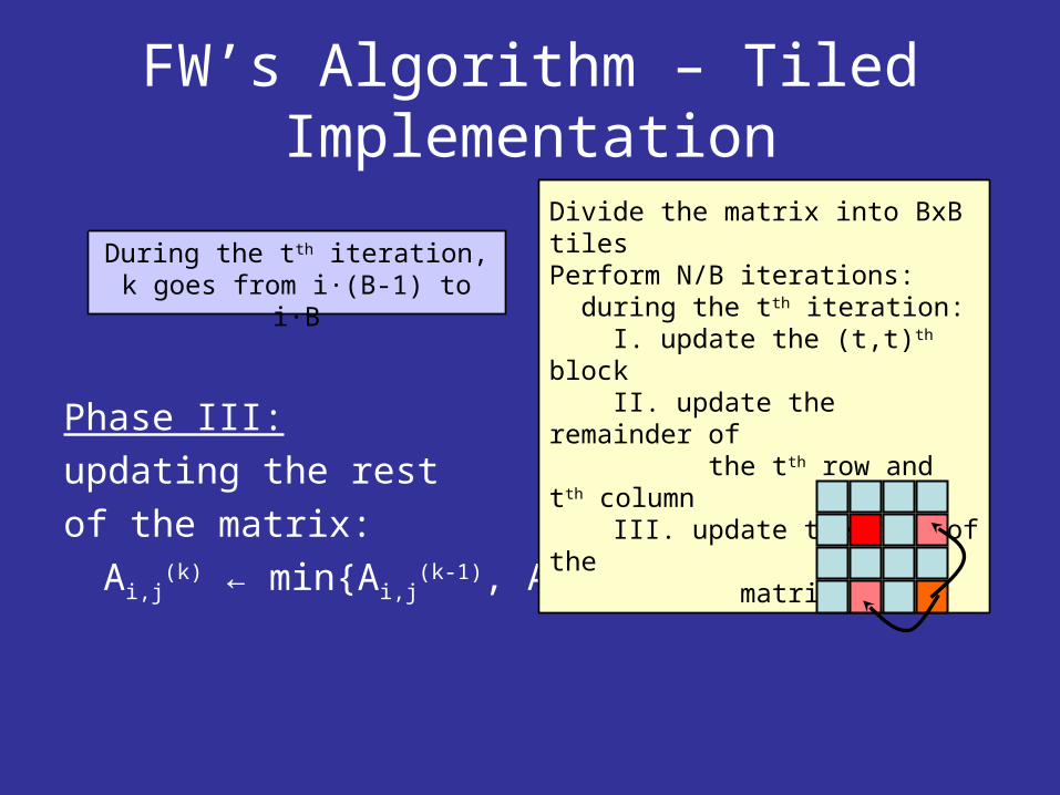
Phase III:updating the rest of the matrix:
Ai,j(k) ← minAi,j
(k-1), Ai,k(tB) + Ak,j
(tB)
Divide the matrix into BxB tilesPerform N/B iterations: during the tth iteration: I. update the (t,t)th block II. update the remainder of the tth row and tth column III. update the rest of the matrix
During the tth iteration, k goes from i·(B-1) to i·B
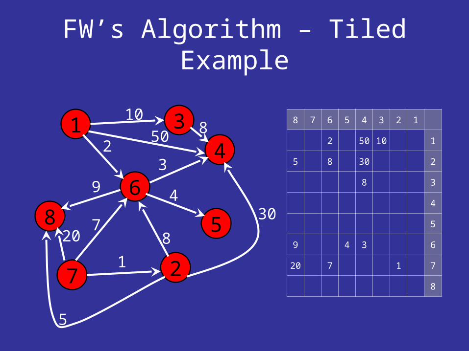
FW’s Algorithm – Tiled Example
1
2
3
68
4
5
7
10
2
30
8
5
8
3
49
1
720
12345678
110502
23085
38
4
5
6349
71720
8
50
FW’s Algorithm – Tiled Example
12345678
110502
23085
38
4
5
6349
717
8
Divide the matrix into BxB tiles
Perform N/B iterations:
during the tth iteration:
I. update the (t,t)th block
II. update the remainder of
the tth row and tth column
III. update the rest of the
matrix206
7-2-8

FW’s Algorithm – Tiled Example
12345678
1102
23085
38
4
5
6349
7176
8
Divide the matrix into BxB tiles
Perform N/B iterations:
during the tth iteration:
I. update the (t,t)th block
II. update the remainder of
the tth row and tth column
III. update the rest of the
matrix
50181-3-4
FW’s Algorithm – Tiled Example
12345678
1102
285
38
4
5
6349
7176
8
Divide the matrix into BxB tiles
Perform N/B iterations:
during the tth iteration:
I. update the (t,t)th block
II. update the remainder of
the tth row and tth column
III. update the rest of the
matrix
6
12
11
1-6-52-6-5
7-6-5
1-6-4 5182-6-43011
111-6-8
7-6-410

FW’s Algorithm – Tiled Example
12345678
11052
21185
38
4
5
6349
7176
8
Divide the matrix into BxB tiles
Perform N/B iterations:
during the tth iteration:
I. update the (t,t)th block
II. update the remainder of
the tth row and tth column
III. update the rest of the
matrix
6
12
11
11
10
Representing the Matrix in an efficient way
In order to match the data access pattern, a tile must be stored in continuous memory.
Therefore, the Z-Morton layout is used.
0123
4567
891011
12131415
0145236789121310111415
FW’s Tiled Algorithm –correctness
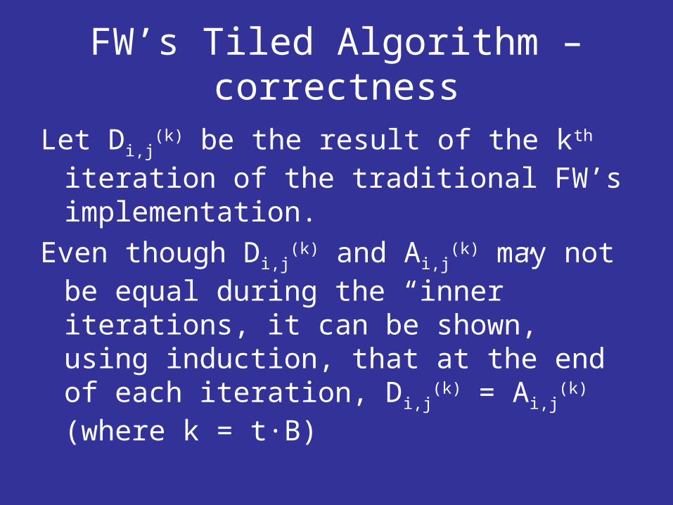
Let Di,j(k) be the result of the kth
iteration of the traditional FW’s implementation.
Even though Di,j(k) and Ai,j
(k) may not be equal during the “inner” iterations, it can be shown, using induction, that at the end of each iteration, Di,j
(k) = Ai,j
(k) (where k = t·B)
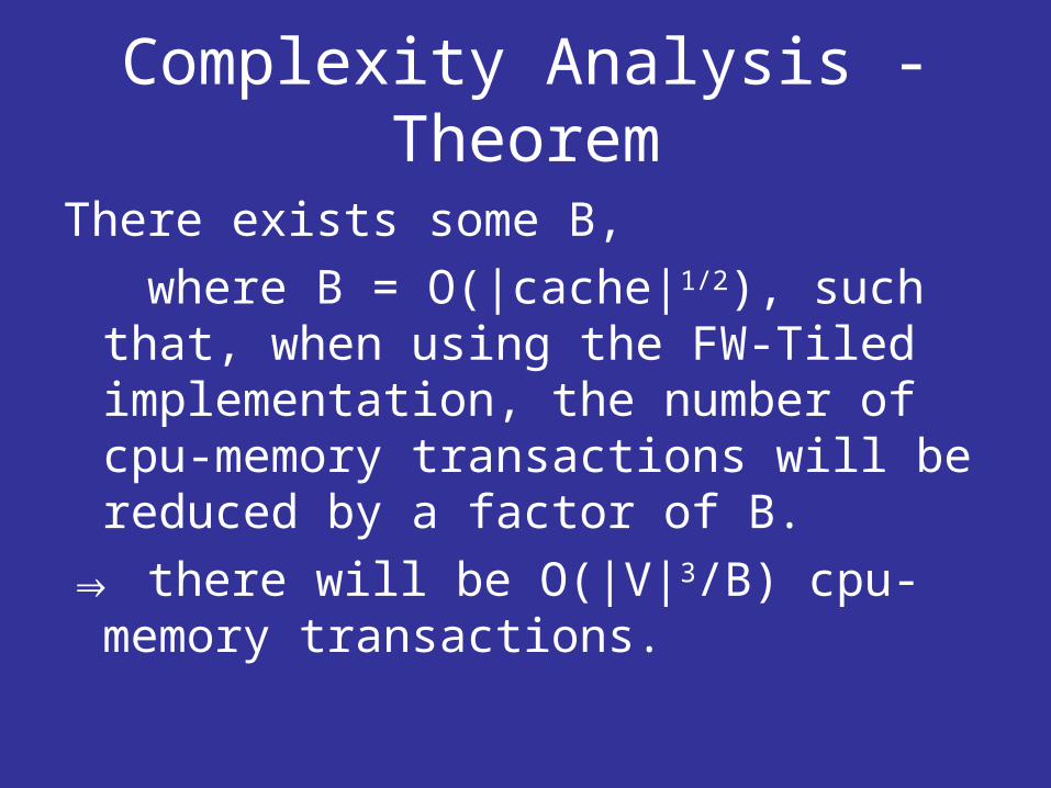
Complexity Analysis - Theorem
There exists some B, where B = O(|cache|1/2), such that,
when using the FW-Tiled implementation, the number of cpu-memory transactions will be reduced by a factor of B.
⇒ there will be O(|V|3/B) cpu-memory transactions.

Complexity Analysis
There are |V|/B x |V|/B tiles in the matrix.
There are |V|/B iterations in the algorithm, in each iteration, all tiles are accessed.
Updating a tile requires holding at most 3 tiles in the cache. ⇒ 3 · B2 ≤ |cache|
Divide the matrix into BxB tilesPerform N/B iterations: during the tth iteration: I. update the (t,t)th block II. update the remainder of the tth row and tth column III. update the rest of the matrix
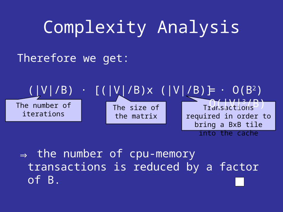
Complexity Analysis
Therefore we get:
(|V|/B) · [(|V|/B)x (|V|/B)] · O(B2)
⇒ the number of cpu-memory transactions is reduced by a factor of B.
The number of iterations
Transactions required in order to bring a BxB tile
into the cache
= O(|V|3/B)
The size of the matrix

Complexity Analysis - Conclusion
The algorithm’s complexity: O(|V|3/B)Lower bound for FW: Ω(|V|3/B) The tiled implementation is
asymptotically optimal among all implementations of the Floyd Warshall algorithm (with respect to cpu-memory transactions).

FW’s Algorithm – Tiled Implementation - Comments
Note, that when using the tiling method, the size of the cache is one of the algorithm’s parameters
Therefore:the tiled algorithm is cache - conscious
FW’s Algorithm – Tiled Implementation - Comments
Since cache parameters have been disregarded, the best (and simplest) way to find the optimal size B is by experiment.
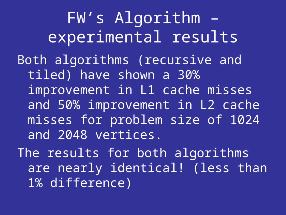
FW’s Algorithm – experimental results
Both algorithms (recursive and tiled) have shown a 30% improvement in L1 cache misses and 50% improvement in L2 cache misses for problem size of 1024 and 2048 vertices.
The results for both algorithms are nearly identical! (less than 1% difference)

Dijkstra’s algorithm for Single Source Shortest Paths & Prim’s Algorithm for
Minimum Spanning Tree
Dijkstra’s Algorithm:S ← ∅Q ← VWhile Q ≠ ∅ u ← extract-min (Q) S ← S ∪ u for each v ∊ adj(u) update d[v]Return S
Prim’s Algorithm:Q ← Vfor each u ∊ Q do key(u) ← ∞key (root) ← 0While Q ≠ ∅ u ← extract-min (Q) for each v ∊ adj(u) if v ∊ Q and weight(u,v) < key(v) than key(v) ← weight(u,v)
Both Algorithms have the same data access pattern
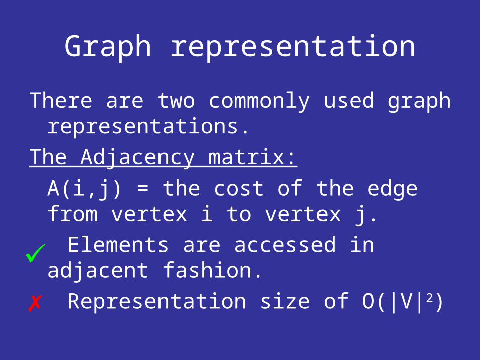
Graph representation
There are two commonly used graph representations.
The Adjacency matrix:A(i,j) = the cost of the edge from vertex i to vertex j.
Elements are accessed in adjacent fashion.
Representation size of O(|V|2)
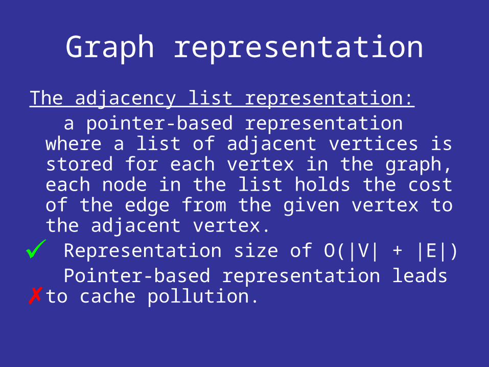
Graph representation
The adjacency list representation: a pointer-based representation where
a list of adjacent vertices is stored for each vertex in the graph, each node in the list holds the cost of the edge from the given vertex to the adjacent vertex.
Representation size of O(|V| + |E|) Pointer-based representation leads to
cache pollution.
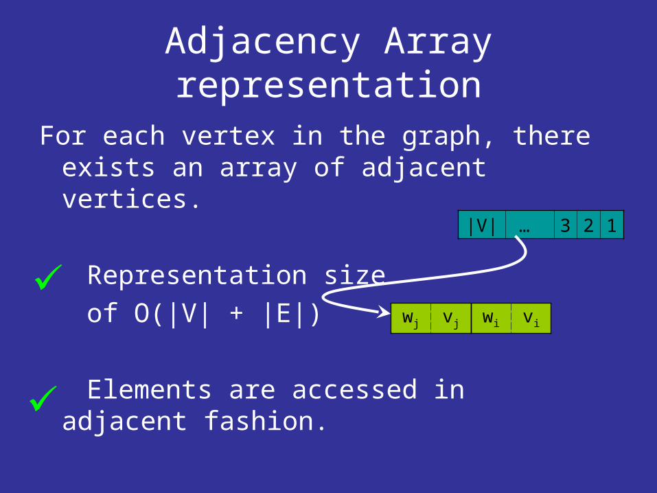
Adjacency Array representation
For each vertex in the graph, there exists an array of adjacent vertices.
Representation size of O(|V| + |E|)
Elements are accessed in adjacent fashion.
123… |V|
viwivjwj
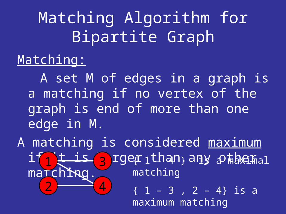
Matching Algorithm for Bipartite Graph
Matching: A set M of edges in a graph is a
matching if no vertex of the graph is end of more than one edge in M.
A matching is considered maximum if it is larger than any other matching.
1
2
3
4
1 – 4 is a maximal matching
1 – 3 , 2 – 4 is a maximum matching
Matching Algorithm for Bipartite Graph
Let M be a matching.All edges in the graph are divided into
two groups: matching-edges and non-matching-edges.
A vertex is called free if it is not an end of any matching edge.

Matching Algorithm for Bipartite Graph
A path P = u0, e1, u1, … , ek, uk is called an augmenting path (with respect to M) if:
- u0 and uk are free.
- the even numbered edges e2, e4, …,
ek-1 are matching edges.
The set of edges M\e2,e4, …,ek-1 ∪ e1,e3, …,ek
is also a matching; it has one edge more than Mhas.So, if we find an augmenting path, we can construct
a larger matching.

Finding Augmenting paths in a Bipartite Graph
In bipartite graphs, each augmenting path has one end in A and one end in B. following such augmenting path starting from its end in A, we traverse non-matching edges from A to B and matching edges from B to A.
By turning the graph into a directed graph (all matching edges are directed vB → vA, all the rest vA → vB), we turn the problem into a simple path finding problem in a directed graph.
Matching Algorithm for Bipartite Graph
The Algorithm:while (there exists an augmenting path)
increase |M| by one using the augmenting path
return MAlgorithm’s complexity: O(|V|·|E|)
Matching Algorithm for Bipartite Graph – first
optimizationIn order to find augmenting paths, we
use the BFS algorithm, which has similar data access pattern to that of Dijsktra/Prim.
Therefore, using the adjacency array instead of the adjacency list / matrix improves running time.

Matching Algorithm for Bipartite Graph – second
optimizationWe try to reduce the size of the
working set as in tiling:I. Partition G into g[1], g[2], … g[p].II. Find the maximum matching in g[i]
for each i ∊ 1,2,.. P using the basic algorithm.
III. Unite all sub-matches into M.IV. Find maximum matching in G using
basic algorithm (starting with M).
Matching Algorithm for Bipartite Graph – second
optimizationIf the sizes of sub-graphs are chosen
appropriately, each of which fits into the cache, it generates minimal cpu-memory transactions of O(|V| + |E|) during phase II, because a single loading of each data element into the cache is necessary.
Finding the best size for a sub-graph is by experiment.
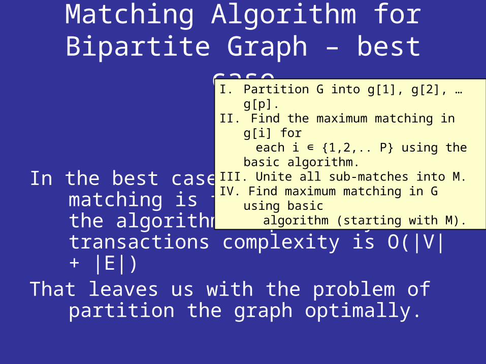
Matching Algorithm for Bipartite Graph – best case
In the best case, the maximum matching is found in phase II, the algorithm’s cpu-memory transactions complexity is O(|V| + |E|)
That leaves us with the problem of partition the graph optimally.
I. Partition G into g[1], g[2], … g[p].II. Find the maximum matching in g[i]
for each i ∊ 1,2,.. P using the basic
algorithm.III. Unite all sub-matches into M.IV. Find maximum matching in G using
basic algorithm (starting with M).
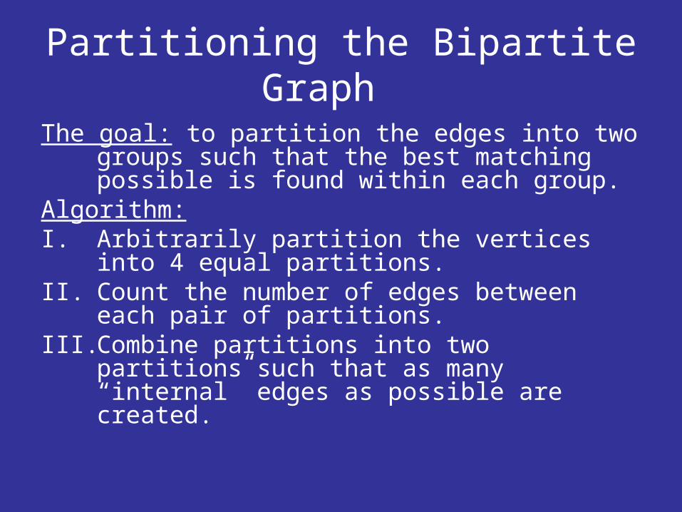
Partitioning the Bipartite Graph
The goal: to partition the edges into two groups such that the best matching possible is found within each group.
Algorithm:I. Arbitrarily partition the vertices into 4
equal partitions.II. Count the number of edges between
each pair of partitions.III. Combine partitions into two partitions
such that as many “internal” edges as possible are created.
Conclusions
Using efficient data representation methods can highly improve algorithms’ running time.
Further improvement can be achieved by methods as tiling and recursion.
Other graph algorithms, such as Bellman-Ford, BFS & DFS can be improved by the above, because of their data access pattern.