Optimizing Energy Efﬁciency for Minimum Latency … Energy...57 Optimizing Energy Efﬁciency for Minimum Latency Broadcast in Low-Duty-Cycle Sensor Networks LIJIE XU, Nanjing University

57

Optimizing Energy Efficiency for Minimum Latency Broadcastin Low-Duty-Cycle Sensor Networks

LIJIE XU, Nanjing University of Posts and TelecommunicationsGUIHAI CHEN, Nanjing UniversityJIANNONG CAO, The Hong Kong Polytechnic UniversitySHAN LIN, Stony Brook UniversityHAIPENG DAI and XIAOBING WU, Nanjing UniversityFAN WU, Shanghai Jiao Tong University

Multihop broadcasting in low-duty-cycle Wireless Sensor Networks (WSNs) is a very challenging problem,since every node has its own working schedule. Existing solutions usually use unicast instead of broadcastto forward packets from a node to its neighbors according to their working schedules, which is, however, notenergy efficient. In this article, we propose to exploit the broadcast nature of wireless media to further saveenergy for low-duty-cycle networks, by adopting a novel broadcasting communication model. The key ideais to let some early wake-up nodes postpone their wake-up slots to overhear broadcasting messages from itsneighbors. This model utilizes the spatiotemporal locality of broadcast to reduce the total energy consump-tion, which can be essentially characterized by the total number of broadcasting message transmissions.Based on such model, we aim at minimizing the total number of broadcasting message transmissions of abroadcast for low-duty-cycle WSNs, subject to the constraint that the broadcasting latency is optimal. Weprove that it is NP-hard to find the optimal solution, and design an approximation algorithm that can achievea polylogarithmic approximation ratio. Extensive simulation results show that our algorithm outperformsthe traditional solutions in terms of energy efficiency.

Categories and Subject Descriptors: C.2.2 [Computer-Communication Networks]: Network Protocols

General Terms: Algorithms, Design

A preliminary version of this article was presented in Proceedings of the 10th IEEE International Conferenceon Mobile Ad-hoc and Sensor Systems (IEEE MASS 2013) [Xu et al. 2013].This work was partly supported by the State Key Development Program for Basic Research of China (973Program) (Grant No. 2012CB316201), National Natural Science Foundation of China (Grants No. 61472252,No. 61321491, No. 61133006, No. 61373130, and No. 61422208), NUPTSF (Grant No. NY214169), NSF ofJiangsu Province (Grant No. BK20141319), EU FP7 CROWN project under Grant No. PIRSES-GA-2013-610524, Funding for Central Institutions of China (No. 20620140515), CCF-Tencent Open Fund, ANR/RGCJoint Research Scheme (RGC No. A-PolyU505/12), NSF CNS-1239108, CNS-1218718, and IIS-1231680.Authors’ addresses: L. Xu, School of Computer Science and Technology, Nanjing University of Posts andTelecommunications, 9 Wenyuan Road, Qixia District, Nanjing 210023, China; email: [email protected]; G.Chen (corresponding author), State Key Laboratory for Novel Software Technology, Nanjing University, 163Xianlin Avenue, Qixia District, Nanjing 210023, China, he is also with Shanghai Key Laboratory of ScalableComputing and Systems, Shanghai Jiao Tong University, 800 Dongchuan Road, Minhang District, Shanghai200240, China; email: [email protected]; J. Cao, Internet and Mobile Computing Lab, The Hong Kong Poly-technic University, Hung Hom, Kowloon, Hong Kong; email: [email protected]; S. Lin, Departmentof Electrical and Computer Engineering, Stony Brook University, Stony Brook, NY 11794-2350, USA; email:[email protected]; H. Dai and X. Wu, State Key Laboratory for Novel Software Technology, Nan-jing University, 163 Xianlin Avenue, Qixia District, Nanjing 210023, China; emails: [email protected],[email protected]; F. Wu, Shanghai Key Laboratory of Scalable Computing and Systems, Shanghai Jiao TongUniversity, 800 Dongchuan Road, Minhang District, Shanghai 200240, China; email: [email protected] to make digital or hard copies of part or all of this work for personal or classroom use is grantedwithout fee provided that copies are not made or distributed for profit or commercial advantage and thatcopies show this notice on the first page or initial screen of a display along with the full citation. Copyrights forcomponents of this work owned by others than ACM must be honored. Abstracting with credit is permitted.To copy otherwise, to republish, to post on servers, to redistribute to lists, or to use any component of thiswork in other works requires prior specific permission and/or a fee. Permissions may be requested fromPublications Dept., ACM, Inc., 2 Penn Plaza, Suite 701, New York, NY 10121-0701 USA, fax +1 (212)869-0481, or [email protected]© 2015 ACM 1550-4859/2015/07-ART57 $15.00

DOI: http://dx.doi.org/10.1145/2753763

ACM Transactions on Sensor Networks, Vol. 11, No. 4, Article 57, Publication date: July 2015.

http://dx.doi.org/10.1145/2753763

57:2 L. Xu et al.

Additional Key Words and Phrases: Wireless sensor networks, low duty cycle, multihop broadcast, energyefficient, minimum broadcasting latency

ACM Reference Format:Lijie Xu, Guihai Chen, Jiannong Cao, Shan Lin, Haipeng Dai, Xiaobing Wu, and Fan Wu. 2015. Optimizingenergy efficiency for minimum latency broadcast in low-duty-cycle sensor networks. ACM Trans. SensorNetw. 11, 4, Article 57 (July 2015), 31 pages.DOI: http://dx.doi.org/10.1145/2753763

1. INTRODUCTION

Wireless Sensor Networks (WSNs) have been widely used for various applications,such as environmental monitoring [Liu et al. 2013a, 2013b; Li and Liu 2009], scientificexploration [Li et al. 2013], and navigation systems [Wang et al. 2013]. Many of theseapplications require broadcasting to frequently disseminate system configurations andcode updates to the whole network. The total energy consumption and the broadcastinglatency are the main performance metrics for evaluation of broadcasting algorithms.

It is important and very challenging to minimize the energy consumption of broad-casting for low-duty-cycle WSNs, in which every sensor node has its own workingschedule to wake up periodically to perform sensing and communication tasks. Ex-isting solutions for broadcasting in low-duty-cycle WSNs (such as Guo et al. [2009],Hong et al. [2010], Wang and Liu [2009], Sun et al. [2009], Niu et al. [2013], Su et al.[2009], Jiao et al. [2010], and Li et al. [2011]) usually implement one-hop broadcastwith multiple unicasts, which is energy inefficient especially for applications of largemessage broadcasting, such as code update. Actually, the broadcast nature of wire-less media offers opportunities to reduce the total number of broadcasting messagetransmissions, even for duty-cycled networks where every node has its own schedule.To improve the energy efficiency of broadcasting, nodes should adjust their workingschedules to maximize the number of receivers for each forwarding message.

Compared with always-awake networks, low-duty-cycle sensor networks usuallyyield a notable increase on communication latency due to periodic sleeping [Gu and He2007], and thus latency is always taken as the first consideration for such networks. Inthis article, we mainly focus on the problem of how to achieve energy-efficient broadcastwith minimum latency for low-duty-cycle WSNs. To achieve optimal latency and highenergy efficiency of broadcasting, we come up with a novel broadcasting communica-tion model, which fully exploits the spatiotemporal locality of broadcasting to reducethe total number of broadcasting message transmissions. The basic idea is to allownodes to adjust their wake-up schedules to overhear forwarding messages sent by theirneighbors. Some nodes may postpone their wake-up slots to receive the broadcastingmessage, increasing their latency. But these nodes can be carefully selected so thatthey are not on latency-critical paths, which indicates their schedule changes do not af-fect the minimum broadcasting latency. Based on such a broadcasting communicationmodel, we find that the total energy consumption for broadcasting can be essentiallycharacterized by the total number of broadcasting message transmissions, and thus ourobjective is to design a broadcast with minimum total number of broadcasting messagetransmissions for low-duty-cycle WSNs, subject to the constraint that the broadcast-ing latency is optimal, which we call the Latency-optimal Minimum Energy BroadcastProblem (LMEB).

The main contributions of this work are as follows:

—To the best of our knowledge, this is the first work that both utilizes the spatiotem-poral locality of broadcasting and proposes a solution with a provable approximation


http://dx.doi.org/10.1145/2753763

Optimizing Energy Efficiency for Minimum Latency Broadcast 57:3

ratio, for energy-efficient broadcast problem with minimum latency constraint inlow-duty-cycle WSNs.

—We prove that the LMEB problem is NP-hard. Then, we model the LMEB problemas the Directed Latency-optimal Group Steiner Tree Problem (DLGST) by capturingthe spatiotemporal characteristic of multihop broadcasting, and propose an efficientsolution for this problem.

—Based on the solution to the DLGST problem, we further devise a novel BroadcastingSchedule Construction Algorithm to derive the solution to the LMEB problem, whichessentially avoids the redundant transmissions and reduces the collision probabilityas much as possible.

—We show that the approximation ratio of our solution is O(log N · log dmax), whereN and dmax denote the number of sensor nodes and the maximum node degree,respectively.

—Extensive simulation results show that our solution makes a significant improve-ment over the traditional solutions in terms of energy efficiency.

The rest of the article is organized as follows: Section 2 summarizes the relatedwork. Section 3 illustrates the network model and formally states the problem. ADetailed descriptions of our proposed scheme and performance analysis are presentedin Section 4, followed by the simulation results and the discussions about practicalissues in Sections 6 and 5, respectively. We conclude the article in Section 7.

2. RELATED WORK

The broadcast problem in low-duty-cycle WSNs has received a lot of attention from theresearch community in the past few years [Guo et al. 2009; Hong et al. 2010; Wang andLiu 2009; Sun et al. 2009; Niu et al. 2013; Su et al. 2009; Jiao et al. 2010; Li et al. 2011;Zhu et al. 2010; Guo et al. 2011; Lai and Ravindran 2010b; Han et al. 2013a, 2013b,2013c; Cheng et al. 2013; Xu and Chen 2013; Kyasanur et al. 2006].

Guo et al. [2009] proposed Opportunistic Flooding to make probabilistic forwardingdecisions at the sender based on the delay distribution of next-hop nodes. Hong et al.[2010] studied the Minimum-Transmission Broadcast Problem in uncoordinated duty-cycled networks and proved its NP-hardness. They proposed a centralized approxima-tion algorithm with a logarithmic approximation ratio and a distributed approximationalgorithm with a constant approximation ratio for this problem. Wang and Liu [2009]proposed a broadcasting scheme to achieve the controllable tradeoff between energyand latency by using a dynamic-programming approach. Another solution ADB [Sunet al. 2009], which is designed to be integrated with the receiver-initiated MAC proto-col [Sun et al. 2008], was proposed to reduce both redundant transmissions and deliverylatency of broadcasting by avoiding collisions and transmissions over poor links. In Niuet al. [2013], the authors investigated the energy-efficient broadcast problem with min-imum latency constraint in low-duty-cycle WSNs with unreliable links, and proposed adistributed heuristic solution to tackle this problem. In Han et al. [2013a], the authorsstudied the duty-cycle-aware Minimum-Energy Multicasting problem in WSNs bothfor one-to-many multicasting and for all-to-all multicasting. Han et al. [2013c] studiedthe problem of minimizing the expected total transmission power for reliable datadissemination in duty-cycled WSNs. Due to the NP-hardness of the problem, theydesigned efficient approximation algorithms with provable performance bounds forit. Cheng et al. [2013] proposed a novel Dynamic Switching-based Reliable Flooding(DSRF) framework, which is designed as an enhancement layer to provide efficientand reliable delivery for a variety of existing flooding tree structures in low duty-cycleWSNs. However, all of these works inefficiently implement one-hop broadcast withmultiple unicasts, which do not fully utilize the spatiotemporal locality of broadcasting.


57:4 L. Xu et al.

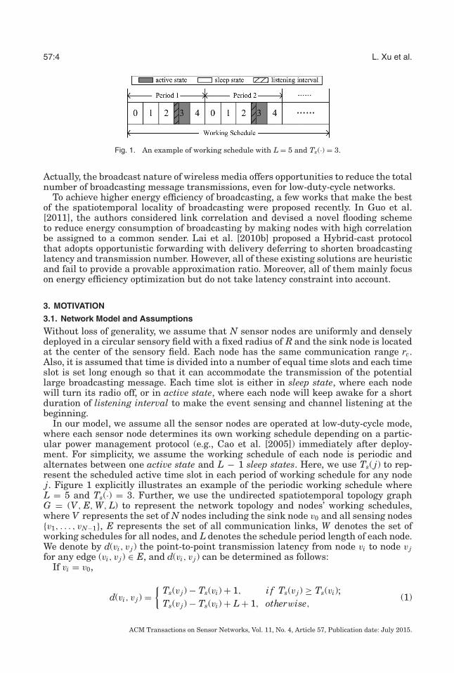
Fig. 1. An example of working schedule with L = 5 and Ts(·) = 3.

Actually, the broadcast nature of wireless media offers opportunities to reduce the totalnumber of broadcasting message transmissions, even for low-duty-cycle networks.

To achieve higher energy efficiency of broadcasting, a few works that make the bestof the spatiotemporal locality of broadcasting were proposed recently. In Guo et al.[2011], the authors considered link correlation and devised a novel flooding schemeto reduce energy consumption of broadcasting by making nodes with high correlationbe assigned to a common sender. Lai et al. [2010b] proposed a Hybrid-cast protocolthat adopts opportunistic forwarding with delivery deferring to shorten broadcastinglatency and transmission number. However, all of these existing solutions are heuristicand fail to provide a provable approximation ratio. Moreover, all of them mainly focuson energy efficiency optimization but do not take latency constraint into account.

3. MOTIVATION

3.1. Network Model and Assumptions

Without loss of generality, we assume that N sensor nodes are uniformly and denselydeployed in a circular sensory field with a fixed radius of R and the sink node is locatedat the center of the sensory field. Each node has the same communication range rc.Also, it is assumed that time is divided into a number of equal time slots and each timeslot is set long enough so that it can accommodate the transmission of the potentiallarge broadcasting message. Each time slot is either in sleep state, where each nodewill turn its radio off, or in active state, where each node will keep awake for a shortduration of listening interval to make the event sensing and channel listening at thebeginning.

In our model, we assume all the sensor nodes are operated at low-duty-cycle mode,where each sensor node determines its own working schedule depending on a partic-ular power management protocol (e.g., Cao et al. [2005]) immediately after deploy-ment. For simplicity, we assume the working schedule of each node is periodic andalternates between one active state and L − 1 sleep states. Here, we use Ts( j) to rep-resent the scheduled active time slot in each period of working schedule for any nodej. Figure 1 explicitly illustrates an example of the periodic working schedule whereL = 5 and Ts(·) = 3. Further, we use the undirected spatiotemporal topology graphG = (V, E, W, L) to represent the network topology and nodes’ working schedules,where V represents the set of N nodes including the sink node v0 and all sensing nodes{v1, . . . , vN−1}, E represents the set of all communication links, W denotes the set ofworking schedules for all nodes, and L denotes the schedule period length of each node.We denote by d(vi, v j) the point-to-point transmission latency from node vi to node v jfor any edge (vi, v j) ∈ E, and d(vi, v j) can be determined as follows:

If vi = v0,

d(vi, v j) ={

Ts(v j) − Ts(vi) + 1, i f Ts(v j) ≥ Ts(vi);Ts(v j) − Ts(vi) + L + 1, otherwise,

(1)



and if vi �= v0,

d(vi, v j) ={

Ts(v j) − Ts(vi), i f Ts(v j) > Ts(vi);Ts(v j) − Ts(vi) + L, otherwise.

(2)

The same as with most literature for low-duty-cycle WSNs (e.g., Guo et al. [2009],Hong et al. [2010], Wang and Liu [2009], Niu et al. [2013], Su et al. [2009], Jiao et al.[2010], Li et al. [2011], Gu and He [2007], Zhu et al. [2010], Guo et al. [2011], Hanet al. [2013a], and Cheng et al. [2013]), we assume time synchronization is achieved,and each node can transmit its packets at any time, while it can only receive the pack-ets from its neighbors in active states. Specifically, each node vi will wake up at thebeginning of the active state and keep listening for a period of listening interval; ifany broadcasting packet in which the target receiver ID is vi is received, it will keepreceiving until all packets of the broadcasting message are received and then go tosleep immediately; otherwise, it will go to sleep immediately. If any sender wants tosend the broadcasting message to its receiver, it will set a timer to wake up itself at thebeginning of the receiver’s next active state to finish the transmission, and then go tosleep.

Besides this, we also have the following basic assumptions:

(1) Each node cannot do sending and receiving simultaneously.(2) Each node is aware of the working schedules of all its neighboring nodes within

two hops; this can be realized via local information exchange between neighboringnodes initially after the network is deployed.

(3) For simplicity, we do not consider the packet collision problem due to the fact thatthe low-duty-cycle operation inherently reduces the probability of collision to agreat extent, which has been experimentally verified in Wang and Liu [2009].

(4) The working schedules of any node and its neighbors are different from each other.It is usually true for low-duty-cycle WSNs, since we usually improve the networkperformance (e.g., to minimize average detection delay) by carefully designing theworking schedules of all nodes (e.g., Cao et al. [2005]) to make the neighboringnodes rotate the sensory coverage. Further, this assumption will be relaxed inSection 4.5.

3.2. Problem Statement

In traditional solutions for broadcasting, all nodes will receive the broadcasting mes-sage at their scheduled wake-up time slots, which could lead to the minimum broad-casting latency but, however, draw much more energy consumption since any one-hopbroadcast is actually realized by a number of unicasts. To achieve higher energy effi-ciency of broadcasting, we come up with a novel broadcasting communication modelthat is based on the spatiotemporal locality of broadcasting. This model defines twokinds of receivers, that is, DelayedReceivers and InstantReceivers, for any sender. Thesender will send the broadcasting message to each InstantReceiver, and also it willsend a short beacon packet that only contains the ID of some InstantReceiver v j , sayBeacon(v j), to each DelayedReceiver. Upon receiving the Beacon(v j) from the sender,any DelayedReceiver will go to sleep immediately and defer its message receiving timeby setting a timer to wake up itself at the next active state of the InstantReceiver v j .Note that, the DelayedReceiver can be aware of the working schedule of the InstantRe-ceiver v j due to the assumption that each node is aware of the working schedules of allits neighboring nodes within two hops.

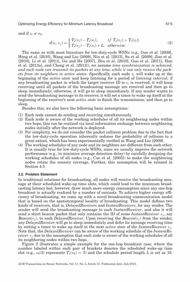
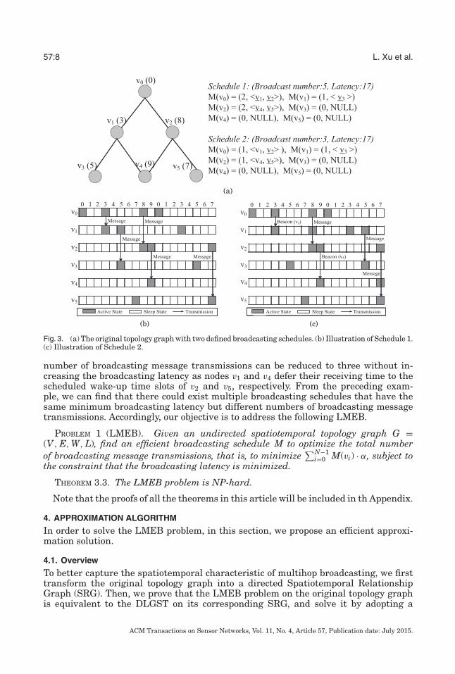
Figure 2 illustrates a simple example for the one-hop broadcast case, where thenumber labeled within each pair of brackets denotes the scheduled wake-up timeslot (e.g., v0(3) represents Ts(v0) = 3) and the schedule period length L is set as 10.


57:6 L. Xu et al.

Fig. 2. (a) Broadcast without deferring. (b) Broadcast with one DelayedReceiver. (c) Broadcast with twoDelayedReceivers. (d) The optimal broadcast.

Figure 2(a) shows a traditional solution, in which the sink node v0 delivers the messageto its neighbors one by one to realize the broadcasting (i.e., to set nodes v1, v2, v3, v4as the InstantReceivers). It requires total energy consumption of Etotal = 4 × k × ed

s +4 × k × ed

r , where k denotes the number of data packets contained in a broadcastingmessage, and ed

s and edr denote the energy consumption when sending and receiving a

data packet, respectively. As shown in Figure 2(b), if the sink node v0 delivers the beaconpacket Beacon(v2) to the DelayedReceiver v1 and delivers the broadcasting message tothe InstantReceivers {v2, v3, v4}, node v1 will defer its message receiving time by settinga timer to wake up itself at the next scheduled active time slot of the InstantReceiverv2 (i.e., time slot 5) and the total energy consumption for broadcasting will be E′

total =eb

s + 3 × k × eds + eb

r + 4 × k × edr , where eb

s and ebr denote the energy consumption when

sending and receiving a beacon packet, respectively. As shown in Wang et al. [2006],it is usual that a data packet has a length of 133 bytes and a beacon packet has onlya length of 19 bytes, which indicates that eb

s + ebr is far less than ed

s in practice. Thus,total energy benefit of deferring the message receiving time of any receiver, that is,� = Etotal − E′

total = k × eds − (eb

s + ebr ), must be greater than zero. For applications

with a large broadcasting message that contains a large number of data packets (i.e.,code update), especially, this benefit will be significant as k � 1. Moreover, we caneasily find that based on such a broadcasting communication model, the total energybenefit will increase as the number of InstantReceivers decreases, which implies thattotal energy consumption for broadcasting can be essentially characterized by totalnumber of broadcasting message transmissions under this model. Figure 2(c) showsan example of broadcast with two DelayedReceivers, that is, the sink node v0 deliversthe beacon packet Beacon(v2) to the DelayedReceiver v1, delivers the beacon packetBeacon(v4) to the DelayedReceiver v3, and delivers the broadcasting message to theInstantReceivers {v2, v4}. According to the previous conclusion, we can find that it musthave a higher energy efficiency than the case in Figure 2(b). Obviously, the schedule inFigure 2(d) must be the optimal solution, where the sink node v0 delivers the beaconpacket Beacon(v4) to the DelayedReceivers {v1, v2, v3} and delivers the broadcastingmessage to the InstantReceiver v4.



According to the previous example, we can find that total energy consumption forbroadcasting will benefit from receive deferring. Based on such a broadcasting commu-nication model, we present the definitions of Forwarding Sequence and BroadcastingSchedule in low-duty-cycle WSNs as follows.

Definition 3.1 (Forwarding Sequence). For any forwarder vi of the broadcastingmessage, its Forwarding Sequence Sf (vi) is defined as a sequence of its receivers sortedbased on the scheduled wake-up time, namely,

Sf (vi) = <[r11 , . . . , rk1

1 ], r1, . . . , [r1j , . . . , rkj

j ], rj>, (3)

where rkj (k = 1, . . . , kj) and the underlined rj , respectively, denote the DelayedReceivers

and InstantReceivers of node vi. Specifically, the forwarder vi will send the short controlpacket Beacon(rj) to each DelayedReceiver rk

j and send the broadcasting message to eachInstantReceiver rj . Here, [ ] denotes an optional item.

Definition 3.2 (Broadcasting Schedule). Given a spatiotemporal topology graph G =(V, E, W, L), the schedule strategy of any node vi ∈ V , say M(vi), can be defined asfollows:

M(vi) = (α, β), (4)

where

α ∈ {0, . . . , N − 1}, β ={

Sf (vi), α > 0;NULL, α = 0.

In Equation (4), the variable α denotes node vi ’s total forwarding number of the broad-casting message, and if vi is the forwarder (i.e., M(vi)·α > 0), β will denote the Forward-ing Sequence Sf (vi), which represents that once receiving the broadcasting message,node vi will send the short beacon packet or the broadcasting message to each node inSf (vi) in sequence. Obviously, M(vi) ·α must be equal to the number of InstantReceiversin Sf (vi). Here, NULL denotes the omitted item and it is obvious that M(vi) ·β = NULLfor any node vi with M(vi) · α = 0. Specifically, it must have M(v0) · α > 0 for the sinknode v0.

Here, a broadcasting schedule M in the network can be defined as the set of all nodes’schedule strategies:

M = {M(vi)|vi ∈ V }, (5)

such that Iα = {vi|vi ∈ V and M(vi) · α > 0} subjects to

(1) connectivity, that is, there must exist a subtree T = (Iα, ET ), where ET ⊆ E andfor any edge (vi, v j) ∈ ET , it must have v j ∈ M(vi) · β if vi is the parent of v j ;

(2) coverage, that is,⋃

vi∈Iα M(vi) · β = V − {v0};(3) nonredundancy, that is, M(vi) · β

⋂M(v j) · β = ∅ for any vi, v j ∈ Iα (i �= j).

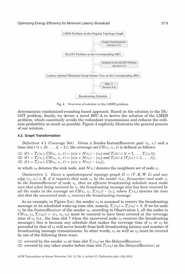
In the preceding definition, note that, we assume each node cannot send the beaconpackets until the broadcasting message is received in order to avoid potential simul-taneous sending and receiving, as well as to simplify the problem. As stated before,we will utilize total number of broadcasting message transmissions to characterizetotal energy consumption for broadcasting. Here, we take two broadcasting schedulesshown in Figure 3 as an example to illustrate our problem. There is no deferring foreach node (i.e., no DelayedReceiver but only InstantReceivers exist in the network)when adopting Schedule 1, which achieves the minimum broadcasting latency 17 butthe maximum number of broadcasting message transmissions 5. For Schedule 2, the


57:8 L. Xu et al.

Fig. 3. (a) The original topology graph with two defined broadcasting schedules. (b) Illustration of Schedule 1.(c) Illustration of Schedule 2.

number of broadcasting message transmissions can be reduced to three without in-creasing the broadcasting latency as nodes v1 and v4 defer their receiving time to thescheduled wake-up time slots of v2 and v5, respectively. From the preceding exam-ple, we can find that there could exist multiple broadcasting schedules that have thesame minimum broadcasting latency but different numbers of broadcasting messagetransmissions. Accordingly, our objective is to address the following LMEB.

PROBLEM 1 (LMEB). Given an undirected spatiotemporal topology graph G =(V, E, W, L), find an efficient broadcasting schedule M to optimize the total numberof broadcasting message transmissions, that is, to minimize

∑N−1i=0 M(vi) · α, subject to

the constraint that the broadcasting latency is minimized.

THEOREM 3.3. The LMEB problem is NP-hard.

Note that the proofs of all the theorems in this article will be included in th Appendix.

4. APPROXIMATION ALGORITHM

In order to solve the LMEB problem, in this section, we propose an efficient approxi-mation solution.

4.1. Overview

To better capture the spatiotemporal characteristic of multihop broadcasting, we firsttransform the original topology graph into a directed Spatiotemporal RelationshipGraph (SRG). Then, we prove that the LMEB problem on the original topology graphis equivalent to the DLGST on its corresponding SRG, and solve it by adopting a



Fig. 4. Overview of solution to the LMEB problem.

deterministic randomized-rounding based approach. Based on the solution to the DL-GST problem, finally, we devise a novel BSC-A to derive the solution of the LMEBproblem, which essentially avoids the redundant transmissions and reduces the colli-sion probability as much as possible. Figure 4 explicitly illustrates the general processof our solution.

4.2. Graph Transformation

Definition 4.1 (Coverage Set). Given a Sender-InstantReceiver pair (vs, vr) and atime slot t (t ∈ {0, . . . , L − 1}), the coverage set CS(vs, vr, t) is defined as follows:

(1) if t < Ts(vr), CS(vs, vr, t) = {x|x ∈ N(vs) − {v0} and Ts(x) ∈ {t + 1, . . . , Ts(vr)}},(2) if t > Ts(vr), CS(vs, vr, t) = {x|x ∈ N(vs) − {v0} and Ts(x) /∈ {Ts(vr) + 1, . . . , t}},(3) if t = Ts(vr), CS(vs, vr, t) = {x|x ∈ N(vs) − {v0}},in which v0 denotes the sink node, and N(vi) denotes the neighbors set of node vi.

OBSERVATION 1. Given a spatiotemporal topology graph G = (V, E, W, L) and anyedge (vs, vr) ∈ E, if it requires that node vs be the sender (i.e., forwarder) and node vrbe the InstantReceiver of node vs, then an efficient broadcasting schedule must makesure that when being received by vr, the broadcasting message also has been received byall the nodes in the coverage set CS(vs, vr, Tc(vs)) − {vr}, where Tc(vs) denotes the timeslot that the uncovered node vs receives the broadcasting message.

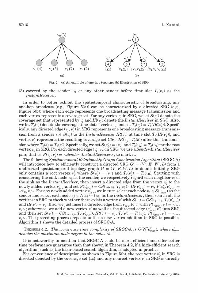
As an example, in Figure 5(a), the sender v0 is assumed to receive the broadcastingmessage at its scheduled wake-up time slot, namely, Tc(v0) = Ts(v0) = 3. If we let nodev3 be the InstantReceiver of the sender v0, according to Observation 1, all the nodes inCS(v0, v3, Tc(v0)) = {v1, v2, v3} must be ensured to have been covered at the coveragetime of v3 (i.e., the time slot 7 when the uncovered node v3 receives the broadcastingmessage); this is because any schedule that makes the coverage time of v1 or v2 bepreceded by that of v3 will never benefit from both broadcasting latency and number ofbroadcasting message transmissions. In other words, v1 as well as v2 must be coveredby one of the following three ways:

(1) covered by the sender v0 at time slot Ts(v3) as the DelayedReceiver;(2) covered by any other sender before time slot Ts(v3) as the DelayedReceiver; or


57:10 L. Xu et al.

Fig. 5. (a) An example of one-hop topology. (b) Illustration of SRG.

(3) covered by the sender v0 or any other sender before time slot Ts(v3) as theInstantReceiver.

In order to better exhibit the spatiotemporal characteristic of broadcasting, anyone-hop broadcast (e.g., Figure 5(a)) can be characterized by a directed SRG (e.g.,Figure 5(b)) where each edge represents one broadcasting message transmission andeach vertex represents a coverage set. For any vertex v′

i in SRG, we let S(v′i) denote the

coverage set that represented by v′i and IR(v′

i) denote the InstantReceiver in S(v′i). Also,

we let Ts(v′i) denote the coverage time slot of vertex v′

i and set Ts(v′i) = Ts(IR(v′

i)). Specif-ically, any directed edge (v′

i, v′j) in SRG represents one broadcasting message transmis-

sion from a sender s ∈ S(v′i) to the InstantReceiver IR(v′

j) at time slot Ts(IR(v′j)), and

vertex v′j represents the resulting coverage set CS(s, IR(v′

j), Tc(s)) after this transmis-sion where Tc(s) = Ts(v′

i). Specifically, we set S(v′0) = {v0} and Ts(v′

0) = Ts(v0) for the rootvertex v′

0 in SRG. For each directed edge (v′i, v

′j) in SRG, we use a Sender-InstantReceiver

pair, that is, P(v′i, v

′j) = <Sender, InstantReceiver>, to mark it.

The following Spatiotemporal Relationship Graph Construction Algorithm (SRGC-A)will introduce how to efficiently construct a directed SRG G′ = (V ′, E′, W ′, L) from aundirected spatiotemporal topology graph G = (V, E, W, L) in detail: Initially, SRGonly contains a root vertex v′

0 where S(v′0) = {v0} and Ts(v′

0) = Ts(v0). Starting withconsidering the sink node v0 as the sender, we respectively regard each neighbor vi ofthe sink as the InstantReceiver, then insert a directed edge from the vertex v′

0 to thenewly added vertex v′

new and set S(v′new) = CS(v0, vi, Ts(v0)), IR(v′

new) = vi, P(v′0, v

′new) =

<v0, vi>. For any newly added vertex v′new, we in turn select each node vi ∈ S(v′

new) as thesender and select each node v j ∈ N(vi)−{v0} as the InstantReceiver, then search all thevertices in SRG to check whether there exists a vertex v′ with S(v′) = CS(vi, v j, Ts(v′

new))and IR(v′) = v j . If so, we just insert a directed edge from v′

new to v′ with P(v′new, v′) = <vi,

v j>; otherwise, we add a new vertex v′ as well as the directed edge (v′new, v′) into SRG

and then set S(v′) = CS(vi, v j, Ts(v′new)), IR(v′) = v j , Ts(v′) = Ts(v j), P(v′

new, v′) = <vi,v j>. The preceding process repeats until no new vertex addition to SRG is possible.Algorithm 1 shows the detailed process of SRGC-A.

THEOREM 4.2. The worst-case time complexity of SRGC-A is O(N2d6max), where dmax

denotes the maximum node degree in the network.

It is noteworthy to mention that SRGC-A could be more efficient and offer bettertime performance guarantee than that shown in Theorem 4.2, if a high-efficient searchalgorithm, such as the hash-based search algorithm, is adopted in practice.

For convenience of description, as shown in Figure 5(b), the root vertex v′0 in SRG is

directed denoted by the coverage set {v0} and any nonroot vertex v′i in SRG is directly



ALGORITHM 1: Spatiotemporal Relationship Graph ConstructionInput: The undirected spatiotemporal topology graph G = (V, E, W, L).Output: The directed spatiotemporal relationship graph G′ = (V ′, E′, W ′, L).V ′ = {v′

0};S(v′

0) = {v0}; Ts(v′0) = Ts(v0); f lag(v′

0) = 1; //v0 ∈ V is the sink nodewhile {v′|v′ ∈ V ′ and f lag(v′) == 1} �= ∅ do

select any vertex v′new ∈ {v′|v′ ∈ V ′ and f lag(v′) == 1};

for each node vi ∈ S(v′new) do

for each node v j ∈ N(vi) − {v0} doisf ound = 0;for each vertex v′ ∈ V ′ do

if S(v′) == CS(vi, v j, Ts(v′new)) and IR(v′) == v j then

add a directed edge (v′new, v′) into E′;

P(v′new, v′) =<vi , v j>;

isf ound = 1; break;end

endif isf ound == 0 then

add a new vertex v′ into V ′;add a directed edge (v′

new, v′) into E′;S(v′) = CS(vi, v j, Ts(v′

new)); IR(v′) = v j ;Ts(v′) = Ts(v j);f lag(v′) = 1;P(v′

new, v′) =<vi , v j>;end

endendf lag(v′

new) = 0;end

denoted by the coverage set S(v′i), in which the underlined node denotes the InstantRe-

ceiver IR(v′i), and the number labeled within any vertex v′

i represents its coverage timeslot Ts(v′

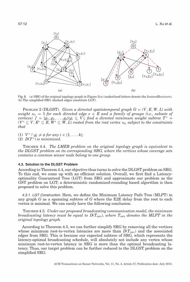
i). We can find that SRG well captures the spatiotemporal characteristic ofbroadcasting and one broadcasting schedule can be implicitly represented by a subtreeof SRG that is rooted from the vertex {v0} and consists of vertices that collectively coverall the nodes in the original topology graph. As an example of multihop broadcasting,Figure 6(a) shows the resulting SRG by performing SRGC-A on the original topologygraph in Figure 3(a).

Next, we first define the DLGST and then show that our target problem can betransformed into the DLGST problem. Essentially, the DLGST problem is a variantof the classic Group Steiner Tree Problem (GST) [Reich and Widmayer 1990]. Givena weighted graph G = (V, E), a root r ∈ V , and a set of groups where each groupis defined as a subset S ⊆ V , the classic GST problem is to find a minimum weightr-rooted subtree containing at least one vertex from each group.

Definition 4.3 (Latency of Tree). Given a spatiotemporal tree T = (V, E, W, L), thelatency of T , say D(T ), can be defined as follows:

D(T ) = maxv∈V −{v0}

{DT (v0, v)}, (6)

where v0 denotes the root of the tree, and DT (i, j) denotes the End-to-End (E2E) latencyfrom vertex i to vertex j on T .


57:12 L. Xu et al.

Fig. 6. (a) SRG of the original topology graph in Figure 3(a) (underlined letters denote the InstantReceivers).(b) The simplified SRG (dashed edges constitute LGT).

PROBLEM 2 (DLGST). Given a directed spatiotemporal graph G = (V, E, W, L) withweight we = 1 for each directed edge e ∈ E and a family of groups (i.e., subsets ofvertices) f = {g1, g2, . . . , gk}(gi ⊆ V ), find a directed minimum weight subtree T ∗ =(V ∗ ⊆ V, E∗ ⊆ E, W∗ ⊆ W, L) rooted from the root vertex v0, subject to the constraintsthat

(1) V ∗ ∩ gi �= φ for any i ∈ {1, . . . , k};(2) D(T ∗) is minimized.

THEOREM 4.4. The LMEB problem on the original topology graph is equivalent tothe DLGST problem on its corresponding SRG, where the vertices whose coverage setscontains a common sensor node belong to one group.

4.3. Solution to the DLGST Problem

According to Theorem 4.4, our objective thus turns to solve the DLGST problem on SRG.To this end, we come up with an efficient solution. Overall, we first find a Latency-optimality Guaranteed Tree (LGT) from SRG and approximate our problem as theGST problem on LGT; a deterministic randomized-rounding based algorithm is thenproposed to solve this problem.

4.3.1. LGT Construction. Here, we define the Minimum Latency Path Tree (MLPT) inany graph G as a spanning subtree of G where the E2E delay from the root to eachvertex is minimal. We can easily have the following conclusion.

THEOREM 4.5. Under our proposed broadcasting communication model, the minimumbroadcasting latency must be equal to D(Tmin), where Tmin denotes the MLPT in theoriginal topology graph.

According to Theorem 4.5, we can further simplify SRG by removing all the verticeswhose minimum root-to-vertex latencies are more than D(Tmin) and the associatededges from SRG. This is because our expected subtree of SRG, which represents thelatency-optimal broadcasting schedule, will absolutely not include any vertex whoseminimum root-to-vertex latency in SRG is more than the optimal broadcasting la-tency. Thus, our target problem can be further reduced to the DLGST problem on thesimplified SRG.



We use OPTGST (T ) and OPTDLGST (G) to denote the cost of the optimal solution forthe GST on any tree T and that for the DLGST problem on any directed graph G,respectively, and the following conclusion holds.

THEOREM 4.6. Given a simplified SRG G′ where the vertices whose coverage setscontains a common sensor node belongs to a group, we must have

OPTGST (T ′) ≤ h(T ′) · OPTDLGST (G′), (7)

where T ′ denotes any latency-optimal spanning subtree of G′ and h(T ′) denotes theheight of tree T ′. Suppose that the parameters R, L, and rc are fixed, then h(T ′) must bebounded by a constant.

For any latency-optimal spanning subtree of the simplified SRG, we call it the LGT.According to Theorem 4.6, obviously, we are expected to find a LGT with lower height toachieve a better performance guarantee. Here, we adopt the following approach, whichis similar to the Bellman-Ford Algorithm, to construct the LGT.

—Initialization: Given a simplified SRG G′, we let Dmin(v′0, v

′i) and hopcount(v′

0, v′i)

denote the minimum E2E latency and the hop count from root v′0 to vertex v′

i, re-spectively. Initially, we set Dmin(v′

0, v′0) = hopcount(v′

0, v′0) = 0, and set Dmin(v′

0, v′i) =

hopcount(v′0, v

′i) = ∞ and p(v′

i) = null for any v′i �= v′

0, where p(v) denotes the parentof vertex v.

—Iteration: For each edge (v′i, v

′j) in G′, if Dmin(v′

0, v′i) + d(v′

i, v′j) < Dmin(v′

0, v′j), we

will update Dmin(v′0, v

′j) = Dmin(v′

0, v′i) + d(v′

i, v′j), hopcount(v′

0, v′j) = hopcount(v′

0, v′i) +

1 and set p(v′j) = v′

i. If Dmin(v′0, v

′i) + d(v′

i, v′j) = Dmin(v′

0, v′j), we will check

whether hopcount(v′0, v

′i) + 1 < hopcount(v′

0, v′j); if so, we update hopcount(v′

0, v′j) =

hopcount(v′0, v

′i) + 1 and set p(v′

j) = v′i. The preceding process is repeated until there

is no update in G′.

For the original topology graph with D(Tmin) = 17 (i.e., Figure 3(a)), we can de-rive the LGT (i.e., Figure 6(b)) by adopting the preceding approach on its SRG (i.e.,Figure 6(a)).

4.3.2. Edge Selection on LGT. As seen previously, accordingly, we can approximate ourproblem as the GST problem on LGT, which has guaranteed the optimality of broad-casting latency. In Garg et al. [1998], the authors proposed an efficient method toaddress the GST Problem on tree. However, Garg et al. [1998] required that the inputtree should be a binary one where each group is a subset of its leaves and groups arepairwise disjoint, and also it only gives a probabilistic solution. Based on the solutionin Garg et al. [1998], we devise a deterministic method, which consists of three steps:

(1) Tree TransformationGiven a LGT T ′ = {V ′, E′, W ′, L}, we first convert T ′ into a binary tree in which

each group is a subset of its leaves and groups are pairwise disjoint via the followingoperations:

—For each internal (i.e., nonroot and nonleaf) vertex v′i in LGT, we insert an edge from

vertex v′i to a newly added vertex v′

new sharing the same S(·) and IR(·) with v′i (i.e.,

S(v′new) = S(v′

i) and IR(v′new) = IR(v′

i)).—For each leaf vertex v′

i in LGT, if |S(v′i)| > 1, we insert |S(v′

i)| edges from v′i to |S(v′

i)|newly added vertices sharing the same S(·) and IR(·) with v′

i.—For each nonleaf vertex v′

i with more than two children, we first add a new vertexv′

new sharing the same S(·) and IR(·) with v′i into LGT; specifically, if v′

i is not the root,we replace v′

i with v′new to be the child of p(v′

i). Then, we delete an edge from v′i to any


57:14 L. Xu et al.

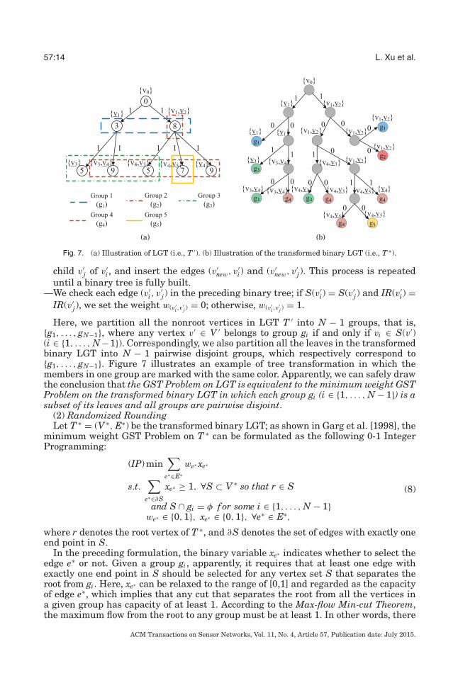
Fig. 7. (a) Illustration of LGT (i.e., T ′). (b) Illustration of the transformed binary LGT (i.e., T ∗).

child v′j of v′

i, and insert the edges (v′new, v′

i) and (v′new, v′

j). This process is repeateduntil a binary tree is fully built.

—We check each edge (v′i, v

′j) in the preceding binary tree; if S(v′

i) = S(v′j) and IR(v′

i) =IR(v′

j), we set the weight w(v′i ,v

′j ) = 0; otherwise, w(v′

i ,v′j ) = 1.

Here, we partition all the nonroot vertices in LGT T ′ into N − 1 groups, that is,{g1, . . . , gN−1}, where any vertex v′ ∈ V ′ belongs to group gi if and only if vi ∈ S(v′)(i ∈ {1, . . . , N−1}). Correspondingly, we also partition all the leaves in the transformedbinary LGT into N − 1 pairwise disjoint groups, which respectively correspond to{g1, . . . , gN−1}. Figure 7 illustrates an example of tree transformation in which themembers in one group are marked with the same color. Apparently, we can safely drawthe conclusion that the GST Problem on LGT is equivalent to the minimum weight GSTProblem on the transformed binary LGT in which each group gi (i ∈ {1, . . . , N − 1}) is asubset of its leaves and all groups are pairwise disjoint.

(2) Randomized RoundingLet T ∗ = (V ∗, E∗) be the transformed binary LGT; as shown in Garg et al. [1998], the

minimum weight GST Problem on T ∗ can be formulated as the following 0-1 IntegerProgramming:

(IP) min∑

e∗∈E∗we∗ xe∗

s.t.∑

e∗∈∂S

xe∗ ≥ 1, ∀S ⊂ V ∗ so that r ∈ S

and S ∩ gi = φ f or some i ∈ {1, . . . , N − 1}we∗ ∈ {0, 1}, xe∗ ∈ {0, 1}, ∀e∗ ∈ E∗,

(8)

where r denotes the root vertex of T ∗, and ∂S denotes the set of edges with exactly oneend point in S.

In the preceding formulation, the binary variable xe∗ indicates whether to select theedge e∗ or not. Given a group gi, apparently, it requires that at least one edge withexactly one end point in S should be selected for any vertex set S that separates theroot from gi. Here, xe∗ can be relaxed to the range of [0,1] and regarded as the capacityof edge e∗, which implies that any cut that separates the root from all the vertices ina given group has capacity of at least 1. According to the Max-flow Min-cut Theorem,the maximum flow from the root to any group must be at least 1. In other words, there



must exist a flow whose value is exactly 1 from the root to any group. Thus, we canrelax the preceding Integer Programming to the following Linear Programming.

(LP) min∑

(u,v)∈E∗w(u,v)x(u,v)

s.t.∑u∈g

∑v∈Vg

fg(v, u) = 1∑(u,v)∈Eg

fg(u, v) =∑

(v,w)∈Eg

fg(v,w), ∀v ∈ Vg − g − {r}

0 ≤ fg(u, v) ≤ x(u,v) ≤ 1, ∀(u, v) ∈ Egw(u,v) ∈ {0, 1}, ∀(u, v) ∈ Eg∀g ∈ {g1, . . . , gN−1},

(9)

where fg denotes the flow from the root to group g and Tg = (Vg, Eg) denotes the subtreeof T ∗, which consists of the paths from the root r to each leaf vertex in group g.

Similar to Garg et al. [1998], we adopt the following approach, which is called theRandomized-rounding based Edge Selection Algorithm (RES-A), to make the edgeselection.

—We define a Selected Edge Set, which is initially set as empty.—We make the following random selection operation: Each edge e∗ in T ∗ is marked with

probability of xe∗xp(e∗ )

, in which xe∗ can be figured out from Equation (9) and p(e∗) denotesthe parent edge of e∗. For any edge e∗ with one end point is the root; specifically, itis marked with probability of xe∗ . An edge is added into the Selected Edge Set if andonly if the edges including itself and all its ancestors are marked.

—We check whether the GST is generated by combining all the edges in the SelectedEdge Set and the zero-weight edges in T ∗; if yes, the edge selection process is ter-minated; otherwise, we repeat the preceding random selection operation until theedge selection is terminated or the random selection operation has been repeated for�η · log(N − 1) · log max1≤i≤N−1 |gi|� rounds, where η is a constant.

The following lemma, which has been proven in Garg et al. [1998], explicitly showsthe performance of the aforementioned randomized-rounding based approach.

LEMMA 4.7 [GARG ET AL. 1998]. For a binary tree in which each group is a subsetof its leaves and groups are pairwise disjoint, the probability that its root fails toreach any group g after one round random selection operation is at most about1 − 1

64 log max1≤i≤N−1 |gi | .

(3) Edge Compensation and ReductionDifferent from Garg et al. [1998], which only gives a probabilistic solution, we will

make sure our solution is deterministic by edge compensation. If the root is not con-nected to some group g after executing RES-A, specifically, we will establish the min-imum weight path from the root to group g and then add the edges on this path thathave not been selected by RES-A into the Selected Edge Set. Finally, we further reducethe solution on the transformed binary LGT to that on the original LGT by removingall the zero-weight edges from the Selected Edge Set.

4.4. Broadcasting Schedule Construction

By adopting the previously mentioned solution, we can approximately obtain the min-imum Group Steiner Tree on LGT that consists of the edges in Selected Edge Set,called T G = (V G, EG, WG, L), which implicitly represents a latency-optimal broad-casting schedule that the total number of broadcasting message transmissions is atmost |EG|. We can easily find that the broadcasting schedule represented by T G must


57:16 L. Xu et al.

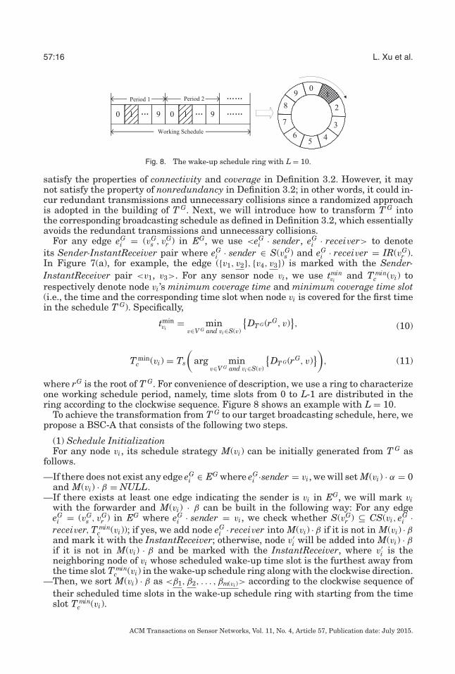
Fig. 8. The wake-up schedule ring with L = 10.

satisfy the properties of connectivity and coverage in Definition 3.2. However, it maynot satisfy the property of nonredundancy in Definition 3.2; in other words, it could in-cur redundant transmissions and unnecessary collisions since a randomized approachis adopted in the building of T G. Next, we will introduce how to transform T G intothe corresponding broadcasting schedule as defined in Definition 3.2, which essentiallyavoids the redundant transmissions and unnecessary collisions.

For any edge eGi = (vG

s , vGr ) in EG, we use <eG

i · sender, eGi · receiver> to denote

its Sender-InstantReceiver pair where eGi · sender ∈ S(vG

s ) and eGi · receiver = IR(vG

r ).In Figure 7(a), for example, the edge ({v1, v2}, {v4, v3}) is marked with the Sender-InstantReceiver pair <v1, v3>. For any sensor node vi, we use tmin

viand T min

c (vi) torespectively denote node vi ’s minimum coverage time and minimum coverage time slot(i.e., the time and the corresponding time slot when node vi is covered for the first timein the schedule T G). Specifically,

tminvi

= minv∈V G and vi∈S(v)

{DT G(rG, v)

}, (10)

T minc (vi) = Ts

(arg min

v∈V G and vi∈S(v)

{DT G(rG, v)

}), (11)

where rG is the root of T G. For convenience of description, we use a ring to characterizeone working schedule period, namely, time slots from 0 to L-1 are distributed in thering according to the clockwise sequence. Figure 8 shows an example with L = 10.

To achieve the transformation from T G to our target broadcasting schedule, here, wepropose a BSC-A that consists of the following two steps.

(1) Schedule InitializationFor any node vi, its schedule strategy M(vi) can be initially generated from T G as

follows.

—If there does not exist any edge eGi ∈ EG where eG

i ·sender = vi, we will set M(vi) · α = 0and M(vi) · β = NULL.

—If there exists at least one edge indicating the sender is vi in EG, we will mark viwith the forwarder and M(vi) · β can be built in the following way: For any edgeeG

i = (vGs , vG

r ) in EG where eGi · sender = vi, we check whether S(vG

r ) ⊆ CS(vi, eGi ·

receiver, T minc (vi)); if yes, we add node eG

i · receiver into M(vi) · β if it is not in M(vi) · βand mark it with the InstantReceiver; otherwise, node v′

i will be added into M(vi) · βif it is not in M(vi) · β and be marked with the InstantReceiver, where v′

i is theneighboring node of vi whose scheduled wake-up time slot is the furthest away fromthe time slot T min

c (vi) in the wake-up schedule ring along with the clockwise direction.—Then, we sort M(vi) · β as <β1, β2, . . . , βm(vi )> according to the clockwise sequence of

their scheduled time slots in the wake-up schedule ring with starting from the timeslot T min

c (vi).



—Finally, we add all the nodes in set CS(vi, βm(vi ), T minc (vi)) − M(vi) · β into M(vi) · β and

mark them with the DelayedReceivers, and then we reorder M(vi) ·β according to theclockwise sequence of their scheduled time slots in the wake-up schedule ring withstarting from the time slot T min

c (vi).

(2) Schedule AdjustmentAfter the previous step, we can get the initial Forwarding Sequence of each forwarder.

However, the broadcasting schedule based on these initial Forwarding Sequences couldincur redundant transmissions and unnecessary collisions, since a randomized ap-proach is adopted in the building of T G. Suppose that we have any three forwarders vi,v j , and vk, of which initial Forwarding Sequences can be represented as follows:

M(vi) · β = <v3, v5, v6, v7, v8, v10, v9>,

M(v j) · β = <v2, v4, v6, v7, v12, v8>,

M(vk) · β = <v5, v1, v6, v11, v8, v9>.(12)

We find that if node v5 receives the broadcasting message from vi no later than thatfrom vk, the transmission from vk to v5 will be redundant and thus v5 can be removedfrom M(vk) ·β. In addition to the redundant transmissions, unnecessary collisions couldalso be inevitable for our derived schedule. For example, the collision would happenwhen the time v6 takes to receive the broadcasting message from v j is the same asthat from vk. If v6 receives the broadcasting message from v j no later than that fromvk, actually, we can get an equivalent Forwarding Sequence by letting v1 in M(vk) · β bethe InstantReceiver and removing v6 from M(vk) · β.

Definition 4.8 (Remove Back). Given any Forwarding Sequence M(vi) · β that containsnode v j , the operation Remove Back v j in M(vi) · β is defined as follows: (1) If v j is theDelayedReceiver, remove v j from M(vi) · β; (2) If v j is the InstantReceiver, replace v jwith the previous node of v j in M(vi) ·β by the InstantReceiver and then remove v j fromit; particularly, if the previous node of v j is also the InstantReceiver or v j is the firstnode in M(vi) · β, just remove v j from M(vi) · β.

In order to satisfy the property of nonredundancy in Definition 3.2, in this step, wepropose the following approach to further adjust M(vi) · α and M(vi) · β values for eachnode vi.

—For each nonsink node vi, we first find the edge eGi = (vG

s , vGr ) in EG such that

vi ∈ S(vGr ) and DT G(rG, vG

r ) = tminvi

, and node eGi · sender is thus selected to be the

candidate sender for vi.—Then, we check the Forwarding Sequence of each forwarder v j where v j �= eG

i · sender;if vi ∈ M(v j) · β, Remove Back vi in M(v j) · β.

—After the previous process, if the new resulting Forwarding Sequence of any forwarderv j is empty, we will set M(v j) · α = 0 and M(v j) · β = NULL.

—For each forwarder v j , finally, we will set M(v j) · α as the number of InstantReceiversin M(v j) · β.

Obviously, the aforementioned approach can ensure each sensing node appears inexactly one forwarder’s Forwarding Sequence, which implies the property of nonredun-dancy in Definition 3.2 must be satisfied. Theorem 4.11 explicitly shows the perfor-mance of our solution.

LEMMA 4.9. Let M∗ denote the resulting broadcasting schedule by performing BSC-Aon T G; we can have that


57:18 L. Xu et al.

(1) M∗ must be latency optimal;

(2)N−1∑i=0

M∗(vi) · α ≤ |EG|.

LEMMA 4.10. log max1≤i≤N−1 |gi| ≤ O(log dmax).

THEOREM 4.11. When η ≥ 64, the approximation ratio of our solution is O(log N ·log dmax).

A straightforward observation from Theorem 4.11 is that we can set the parameterη as 64 in our solution to guarantee a polylogarithmic approximation ratio.

4.5. Extension

Note that we assumed the working schedules of neighboring nodes are different fromeach other, which is commonly seen in low-duty-cycle WSNs. Nevertheless, our solutioncan also be extended to the generalized case where a few of the neighboring nodes couldhave the identical wake-up schedule, by simply regarding the set of neighbors havingidentical wake-up time slot as one virtual node. For example, the initial ForwardingSequence of forwarder vi can be represented as follows.

M(vi) · β = <{v3, v5}, v6, v7, {v8, v10, v9}>, (13)

where {v3, v5} and {v8, v10, v9} denote two virtual nodes, that is, Ts(v3) = Ts(v5) andTs(v8) = Ts(v10) = Ts(v9). Here, a virtual node is called the DelayedReceiver (InstantRe-ceiver) if and only if all sensor nodes in this virtual node are the DelayedReceivers(InstantReceivers), and any InstantReceiver virtual node in M(vi) · β represents onebroadcasting message transmission.

In BSC-A, a virtual node is Removed Back in the Forwarding Sequence of any for-warder vi if and only if node vi is not the candidate sender for each node in this virtualnode. Otherwise, we only need to remove the sensor nodes whose candidate sendersare not vi from the virtual node.

5. PRACTICAL ISSUES

In this section, we will discuss the practical issues faced when implementing ourproposed solution.

Note that, we make the same assumptions as most of the existing works aboutbroadcast scheduling for low-duty-cycle WSNs; that is, the assumptions made in ourarticle are all commonly used in the existing related works and our solution does NOTbring any additional overhead compared with the existing related works. Actually,these commonly used assumptions will cost much less overhead in practice. For exam-ple, we only need to realize a local synchronization between neighboring nodes in ourarticle. In real WSNs, local synchronization can be achieved by using an existing high-efficient MAC-layer time stamping technique, Flooding Time Synchronization Protocol(FTSP) [Maroti et al. 2004], which achieves an accuracy of 2.24us with the cost ofexchanging only a few bytes of packets among neighboring nodes every 15 minutes.Since the length of each time slot is usually long enough (at least tens of milliseconds)in practice, the accuracy of 2.24us is sufficient. Also, the assumption that each nodeis aware of the working schedules of all its neighboring nodes within two hops canbe realized by just exchanging the schedules between neighboring nodes twice in theinitialization phase of the network. Specifically, each node will initially keep awake anddetermine its own working schedule according to a particular power management pro-tocol immediately after the deployment, and then exchange the working schedule withits neighbors. Once getting the information about all its neighbors’ working schedules,each node will deliver it to each of its neighbors again. In our solution, we will use a



binary string to represent the working schedule, for example, to use the binary string<0010> to represent the periodic working schedule with Ts(·) = 2 and L = 4. In thisway, we can find that the exchange cost of the working schedules between neighboringnodes is quite low especially when an efficient string compression scheme is adopted.More importantly, this exchange is only a one-time task during the implementation ofour solution. Therefore, this assumption will bring much less overhead in practice.

Upon getting the information about the working schedules of all the neighbors, eachnode will deliver it to the sink immediately. The sink will derive the spatiotemporalnetwork topology graph based on the collected information from all nodes, then executeour centralized algorithm to obtain the broadcasting schedule and distribute it to eachnode in the network. This will be done during the initialization phase of the networkand is a one-time task. Actually, this is also the commonly used implementation formost of the existing centralized algorithms. Once getting the transmission strategy,each node will put itself into the low-duty-cycle mode according to its own workingschedule. Upon receiving a packet, any node v will check its header to see whetherit is a broadcast packet; if yes, node v will forward this packet according to its owntransmission strategy.

In this article, we assume that our target applications will not experience a notablechange on the link qualities, which implies that the topology changes mainly come fromthe energy depletion of sensing nodes. In practice, some emerging technologies (e.g.,Wireless Charging Technology [Dai et al. 2014] and Mobile Robot Technology [Fletcheret al. 2010]) can help us deal with such kind of topology changes. For example, we canset an energy threshold for each node, and any node will transmit an alarm packetto the sink once its residual energy is below this threshold. Upon receiving the alarmpacket, the sink will send a mobile charger to the target node and wirelessly rechargeit, or send a mobile robot there to replace the target node with a new one that hasthe same code and configuration as the target node. In this case, we do not need toconsider the topology change and the network initialization phase is just a one-timetask, which implies the control traffic in the network initialization phase will bringmuch less overhead compared with the long-term run of the broadcasting applicationsso that its cost can be approximately neglected.

6. PERFORMANCE EVALUATION

In this section, we evaluate the performance of our solution via simulations.In our setting, we assume sensor nodes are uniformly distributed in a circular sensory

field with a radius of R = 50m and the sink node is located at the center of the sensoryfield. For simplicity, we assume that one period of any node’s working schedule containsonly one active state time slot and we let each sensing node independently and randomlydetermine its own working schedule. For the sink node v0, specifically, we set Ts(v0) = 0.Further, we adopt the following classic energy consumption model that is commonlyused in much of the existing literature such as Heinzelman et al. [2000]:

es(l) = l · Eelec + l · εampr2c , er(l) = l · Eelec, (14)

where Eelec = 50nJ/bit, εamp = 100pJ/bit/m2, l denotes the packet length, and es(l)and er(l) denote the energy consumed by sending a packet and receiving a packet,respectively. The same as with literature [Wang et al. 2006], we define that each datapacket and each beacon packet have a length of 133 bytes and 19 bytes, respectively.Unless otherwise stated, we set N = 300, L = 100, rc = 10m, and all the results areobtained by averaging over 10 experiments.

Here, we take the following two approaches as the baselines to evaluate the perfor-mance of our solution.


57:20 L. Xu et al.

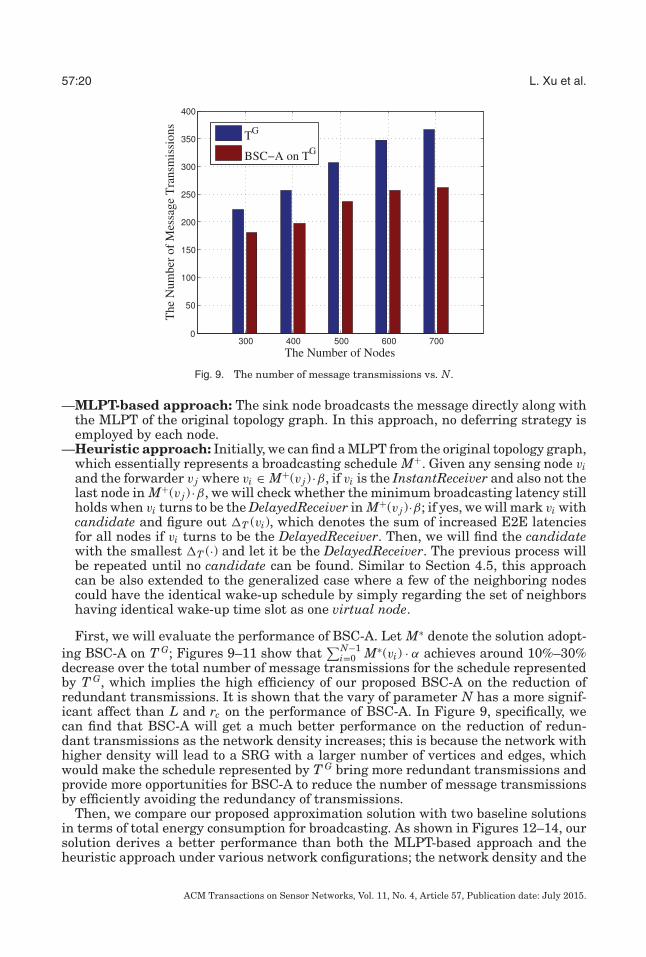
Fig. 9. The number of message transmissions vs. N.

—MLPT-based approach: The sink node broadcasts the message directly along withthe MLPT of the original topology graph. In this approach, no deferring strategy isemployed by each node.

—Heuristic approach: Initially, we can find a MLPT from the original topology graph,which essentially represents a broadcasting schedule M+. Given any sensing node viand the forwarder v j where vi ∈ M+(v j) ·β, if vi is the InstantReceiver and also not thelast node in M+(v j) ·β, we will check whether the minimum broadcasting latency stillholds when vi turns to be the DelayedReceiver in M+(v j)·β; if yes, we will mark vi withcandidate and figure out �T (vi), which denotes the sum of increased E2E latenciesfor all nodes if vi turns to be the DelayedReceiver. Then, we will find the candidatewith the smallest �T (·) and let it be the DelayedReceiver. The previous process willbe repeated until no candidate can be found. Similar to Section 4.5, this approachcan be also extended to the generalized case where a few of the neighboring nodescould have the identical wake-up schedule by simply regarding the set of neighborshaving identical wake-up time slot as one virtual node.

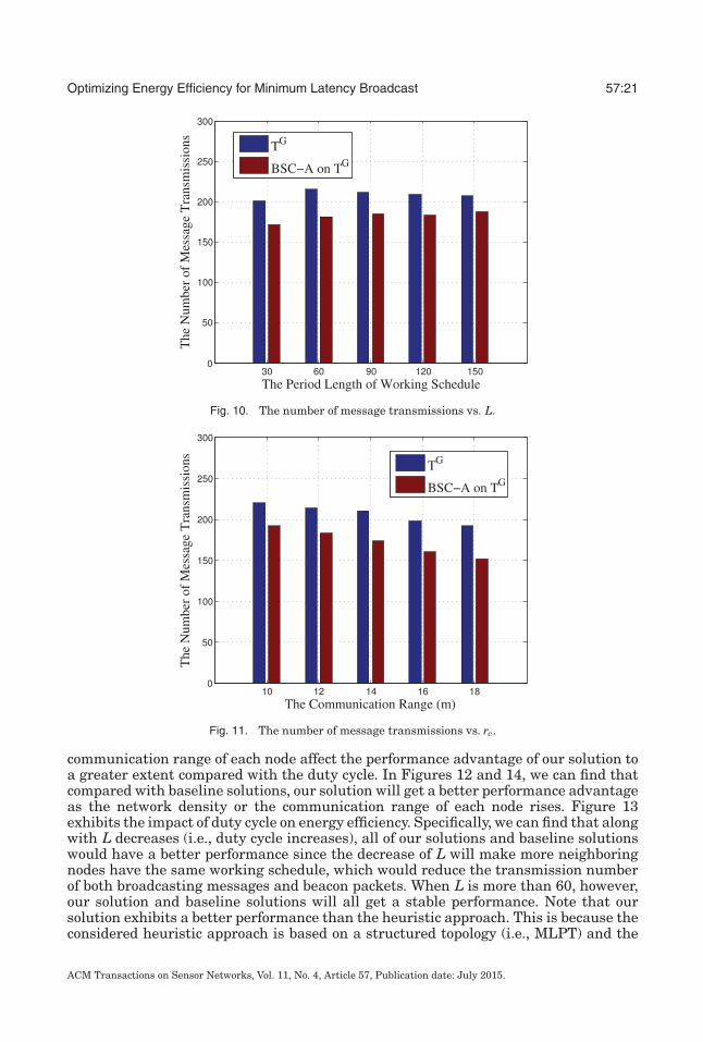
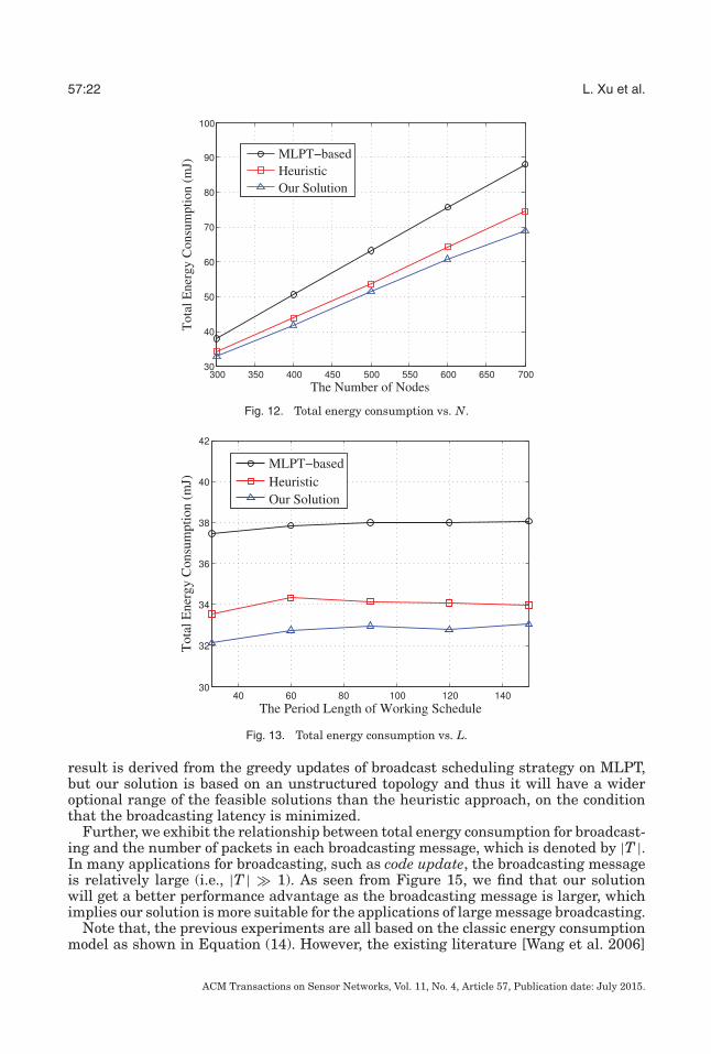
First, we will evaluate the performance of BSC-A. Let M∗ denote the solution adopt-ing BSC-A on T G; Figures 9–11 show that

∑N−1i=0 M∗(vi) · α achieves around 10%–30%

decrease over the total number of message transmissions for the schedule representedby T G, which implies the high efficiency of our proposed BSC-A on the reduction ofredundant transmissions. It is shown that the vary of parameter N has a more signif-icant affect than L and rc on the performance of BSC-A. In Figure 9, specifically, wecan find that BSC-A will get a much better performance on the reduction of redun-dant transmissions as the network density increases; this is because the network withhigher density will lead to a SRG with a larger number of vertices and edges, whichwould make the schedule represented by T G bring more redundant transmissions andprovide more opportunities for BSC-A to reduce the number of message transmissionsby efficiently avoiding the redundancy of transmissions.

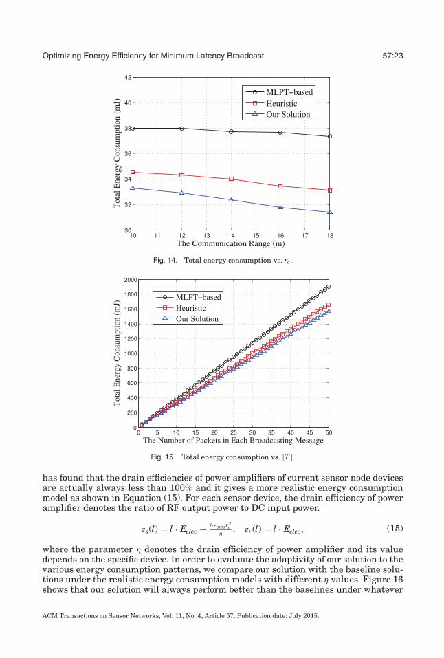
Then, we compare our proposed approximation solution with two baseline solutionsin terms of total energy consumption for broadcasting. As shown in Figures 12–14, oursolution derives a better performance than both the MLPT-based approach and theheuristic approach under various network configurations; the network density and the



Fig. 10. The number of message transmissions vs. L.

Fig. 11. The number of message transmissions vs. rc.

communication range of each node affect the performance advantage of our solution toa greater extent compared with the duty cycle. In Figures 12 and 14, we can find thatcompared with baseline solutions, our solution will get a better performance advantageas the network density or the communication range of each node rises. Figure 13exhibits the impact of duty cycle on energy efficiency. Specifically, we can find that alongwith L decreases (i.e., duty cycle increases), all of our solutions and baseline solutionswould have a better performance since the decrease of L will make more neighboringnodes have the same working schedule, which would reduce the transmission numberof both broadcasting messages and beacon packets. When L is more than 60, however,our solution and baseline solutions will all get a stable performance. Note that oursolution exhibits a better performance than the heuristic approach. This is because theconsidered heuristic approach is based on a structured topology (i.e., MLPT) and the


57:22 L. Xu et al.

Fig. 12. Total energy consumption vs. N.

Fig. 13. Total energy consumption vs. L.

result is derived from the greedy updates of broadcast scheduling strategy on MLPT,but our solution is based on an unstructured topology and thus it will have a wideroptional range of the feasible solutions than the heuristic approach, on the conditionthat the broadcasting latency is minimized.

Further, we exhibit the relationship between total energy consumption for broadcast-ing and the number of packets in each broadcasting message, which is denoted by |T |.In many applications for broadcasting, such as code update, the broadcasting messageis relatively large (i.e., |T | � 1). As seen from Figure 15, we find that our solutionwill get a better performance advantage as the broadcasting message is larger, whichimplies our solution is more suitable for the applications of large message broadcasting.

Note that, the previous experiments are all based on the classic energy consumptionmodel as shown in Equation (14). However, the existing literature [Wang et al. 2006]



Fig. 14. Total energy consumption vs. rc.

Fig. 15. Total energy consumption vs. |T |.

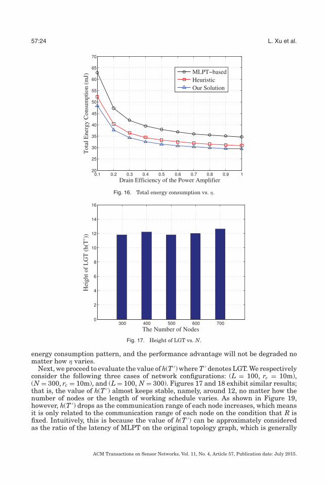
has found that the drain efficiencies of power amplifiers of current sensor node devicesare actually always less than 100% and it gives a more realistic energy consumptionmodel as shown in Equation (15). For each sensor device, the drain efficiency of poweramplifier denotes the ratio of RF output power to DC input power.

es(l) = l · Eelec + l·εampr2c

η, er(l) = l · Eelec, (15)

where the parameter η denotes the drain efficiency of power amplifier and its valuedepends on the specific device. In order to evaluate the adaptivity of our solution to thevarious energy consumption patterns, we compare our solution with the baseline solu-tions under the realistic energy consumption models with different η values. Figure 16shows that our solution will always perform better than the baselines under whatever


57:24 L. Xu et al.

Fig. 16. Total energy consumption vs. η.

Fig. 17. Height of LGT vs. N.

energy consumption pattern, and the performance advantage will not be degraded nomatter how η varies.

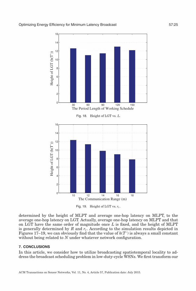
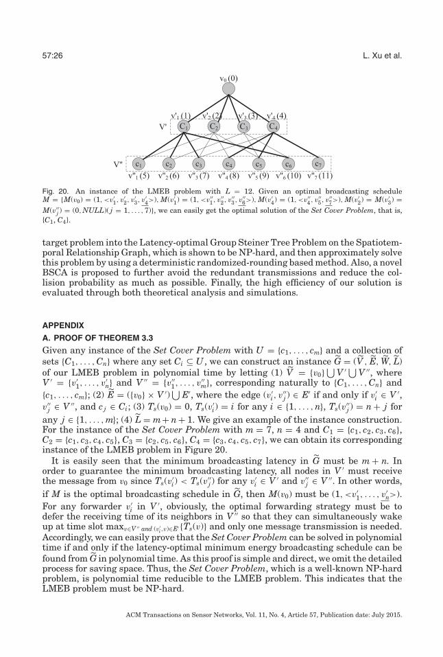
Next, we proceed to evaluate the value of h(T ′) where T ′ denotes LGT. We respectivelyconsider the following three cases of network configurations: (L = 100, rc = 10m),(N = 300, rc = 10m), and (L = 100, N = 300). Figures 17 and 18 exhibit similar results;that is, the value of h(T ′) almost keeps stable, namely, around 12, no matter how thenumber of nodes or the length of working schedule varies. As shown in Figure 19,however, h(T ′) drops as the communication range of each node increases, which meansit is only related to the communication range of each node on the condition that R isfixed. Intuitively, this is because the value of h(T ′) can be approximately consideredas the ratio of the latency of MLPT on the original topology graph, which is generally



Fig. 18. Height of LGT vs. L.

Fig. 19. Height of LGT vs. rc.

determined by the height of MLPT and average one-hop latency on MLPT, to theaverage one-hop latency on LGT. Actually, average one-hop latency on MLPT and thaton LGT have the same order of magnitude once L is fixed, and the height of MLPTis generally determined by R and rc. According to the simulation results depicted inFigures 17–19, we can obviously find that the value of h(T ′) is always a small constantwithout being related to N under whatever network configuration.

7. CONCLUSIONS

In this article, we consider how to utilize broadcasting spatiotemporal locality to ad-dress the broadcast scheduling problem in low-duty-cycle WSNs. We first transform our


57:26 L. Xu et al.

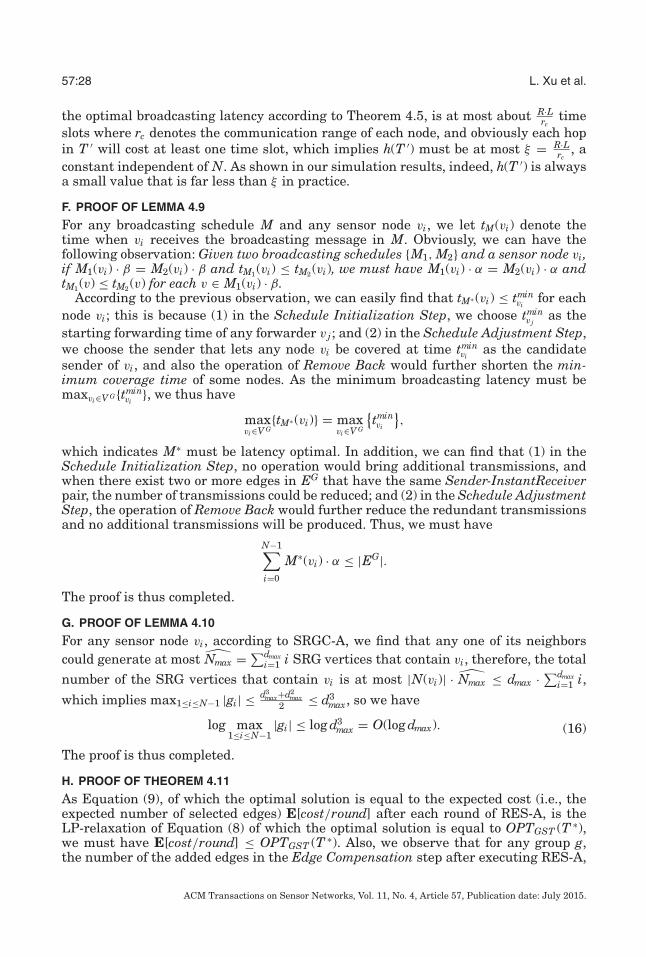
Fig. 20. An instance of the LMEB problem with L = 12. Given an optimal broadcasting scheduleM = {M(v0) = (1, <v′

1, v′2, v′

3, v′4>), M(v′

1) = (1, <v′′1, v′′

2, v′′3, v′′

6>), M(v′4) = (1, <v′′

4, v′′5, v′′

7>), M(v′2) = M(v′

3) =M(v′′

j ) = (0, NULL)( j = 1, . . . , 7)}, we can easily get the optimal solution of the Set Cover Problem, that is,{C1, C4}.

target problem into the Latency-optimal Group Steiner Tree Problem on the Spatiotem-poral Relationship Graph, which is shown to be NP-hard, and then approximately solvethis problem by using a deterministic randomized-rounding based method. Also, a novelBSCA is proposed to further avoid the redundant transmissions and reduce the col-lision probability as much as possible. Finally, the high efficiency of our solution isevaluated through both theoretical analysis and simulations.

APPENDIX

A. PROOF OF THEOREM 3.3

Given any instance of the Set Cover Problem with U = {c1, . . . , cm} and a collection ofsets {C1, . . . , Cn} where any set Ci ⊆ U , we can construct an instance G = (V , E, W, L)of our LMEB problem in polynomial time by letting (1) V = {v0}

⋃V ′ ⋃ V ′′, where

V ′ = {v′1, . . . , v

′n} and V ′′ = {v′′

1, . . . , v′′m}, corresponding naturally to {C1, . . . , Cn} and

{c1, . . . , cm}; (2) E = ({v0} × V ′)⋃

E′, where the edge (v′i, v

′′j ) ∈ E′ if and only if v′

i ∈ V ′,v′′

j ∈ V ′′, and c j ∈ Ci; (3) Ts(v0) = 0, Ts(v′i) = i for any i ∈ {1, . . . , n}, Ts(v′′

j ) = n + j forany j ∈ {1, . . . , m}; (4) L = m+ n + 1. We give an example of the instance construction.For the instance of the Set Cover Problem with m = 7, n = 4 and C1 = {c1, c2, c3, c6},C2 = {c1, c3, c4, c5}, C3 = {c2, c5, c6}, C4 = {c3, c4, c5, c7}, we can obtain its correspondinginstance of the LMEB problem in Figure 20.

It is easily seen that the minimum broadcasting latency in G must be m + n. Inorder to guarantee the minimum broadcasting latency, all nodes in V ′ must receivethe message from v0 since Ts(v′

i) < Ts(v′′j ) for any v′

i ∈ V ′ and v′′j ∈ V ′′. In other words,

if M is the optimal broadcasting schedule in G, then M(v0) must be (1,<v′1, . . . , v

′n>).

For any forwarder v′i in V ′, obviously, the optimal forwarding strategy must be to

defer the receiving time of its neighbors in V ′′ so that they can simultaneously wakeup at time slot maxv∈V ′′ and (v′

i ,v)∈E′ {Ts(v)} and only one message transmission is needed.Accordingly, we can easily prove that the Set Cover Problem can be solved in polynomialtime if and only if the latency-optimal minimum energy broadcasting schedule can befound from G in polynomial time. As this proof is simple and direct, we omit the detailedprocess for saving space. Thus, the Set Cover Problem, which is a well-known NP-hardproblem, is polynomial time reducible to the LMEB problem. This indicates that theLMEB problem must be NP-hard.



B. PROOF OF THEOREM 4.2

Seeing from SRGC-A, we find that the vertex search operation actually dominatesthe whole construction procedure of SRG. In SRGC-A, it results in at most d2

max SRGvertices for any node in G where dmax denotes the maximum node degree in G, thus,there are in total at most N · d2

max vertices in SRG. We assume there are ultimately xvertices in SRG after executing SRGC-A (x ≤ N · d2

max). As we know, the size of anyvertex’s coverage set is at most dmax, which means any vertex will result in at most d2

maxedges and the total number of edges in SRG is thus at most x · d2

max. Actually, we candivide all the edges in SRG into two categories: (1) x − 1 edges, which are connected tothe new added vertices after the search operation; and (2) x · d2

max − x + 1 edges, whichare connected to the existing vertices after the search operation. The total search timefor the first category is at most

∑x−2m=0 m = (x−2)(x−1)

2 , and that for the second category isat most (x − 1)(x · d2

max − x + 1).Due to the fact that x ≤ N ·d2

max, the total search time of SRGC-A is therefore at most(x−2)(x−1)

2 + (x − 1)(x · d2max − x + 1) = O(x2d2

max) ≤ O(N2d6max).

C. PROOF OF THEOREM 4.4

In SRG, we can partition all the nonroot vertices into N − 1 groups according to thecommon members involved in their coverage sets. Here, we let G denote the originaltopology graph and G′ denote its corresponding SRG. For any node vi in G, specifically,any vertex v′ in G′ belongs to group gi if and only if vi ∈ S(v′), where i ∈ {1, . . . , N − 1}.Consequently, one broadcasting schedule can be implicitly represented by a subtreeof SRG that is rooted from the vertex {v0} and connects at least one vertex in eachgroup of SRG. We can easily find that for any latency-optimal broadcast scheduling Min G, it can be characterized by a corresponding Latency-optimal Group Steiner TreeT = (VT , ET ) in G′, where

∑N−1i=0 M(vi) · α = |ET |. Also, it is easily seen that for any

Latency-optimal Group Steiner Tree T = (VT , ET ) in G′, it can be transformed into alatency-optimal broadcast scheduling M, where

∑N−1i=0 M(vi) · α ≤ |ET |. This indicates

the cost of the optimal solution for the LMEB problem on G must be equal to that forthe DLGST problem on G′. Thus, the proof is completed.

D. PROOF OF THEOREM 4.5

Actually, Tmin can be regarded as a broadcasting schedule without waiting. Assumethat node vb is the leaf on Tmin of which sink-to-node latency DT (v0, vb) is the maximumoverall. Obviously, we cannot find a broadcasting schedule whose latency is less thanDT (v0, vb), given that the schedule guarantees vb is covered. This is because the E2Elatency will not benefit from waiting in duty-cycled WSNs, which has been shown in Laiand Ravindran [2010a]. Thus, the optimal broadcasting latency must be DT (v0, vb). AsDT (v0, vb) = D(Tmin), the proof is completed.

E. PROOF OF THEOREM 4.6

We denote by Topt = (VT , ET ) the optimal solution of our target problem. Given anylatency-optimal spanning subtree T ′, it is easy to see that the subtree of T ′ containingall the vertices in VT −{r} (r denotes the root vertex), say T = (V , E), must be a feasiblesolution. For the worst case in which all the vertices in VT − {r} are just the leaves ofT ′, we have OPTGST (T ′) ≤ |E| ≤ ∑

i∈VT −{r} |Path(r, i)| ≤ h(T ′) · |VT −{r}| = h(T ′) · |ET | =h(T ′) ·OPTDLGST (G′), where |Path(r, i)| denotes the hop count of the path from root r tovertex i. As all nodes are assumed to be uniformly and densely deployed in the sensoryfield, we can easily find that the latency of MLPT in the original topology graph, that is,


57:28 L. Xu et al.

the optimal broadcasting latency according to Theorem 4.5, is at most about R·Lrc

timeslots where rc denotes the communication range of each node, and obviously each hopin T ′ will cost at least one time slot, which implies h(T ′) must be at most ξ = R·L

rc, a

constant independent of N. As shown in our simulation results, indeed, h(T ′) is alwaysa small value that is far less than ξ in practice.

F. PROOF OF LEMMA 4.9

For any broadcasting schedule M and any sensor node vi, we let tM(vi) denote thetime when vi receives the broadcasting message in M. Obviously, we can have thefollowing observation: Given two broadcasting schedules {M1, M2} and a sensor node vi ,if M1(vi) · β = M2(vi) · β and tM1 (vi) ≤ tM2 (vi), we must have M1(vi) · α = M2(vi) · α andtM1 (v) ≤ tM2 (v) for each v ∈ M1(vi) · β.

According to the previous observation, we can easily find that tM∗ (vi) ≤ tminvi

for eachnode vi; this is because (1) in the Schedule Initialization Step, we choose tmin

v jas the

starting forwarding time of any forwarder v j ; and (2) in the Schedule Adjustment Step,we choose the sender that lets any node vi be covered at time tmin

vias the candidate

sender of vi, and also the operation of Remove Back would further shorten the min-imum coverage time of some nodes. As the minimum broadcasting latency must bemaxvi∈V G{tmin

vi}, we thus have

maxvi∈V G

{tM∗(vi)} = maxvi∈V G

{tminvi

},

which indicates M∗ must be latency optimal. In addition, we can find that (1) in theSchedule Initialization Step, no operation would bring additional transmissions, andwhen there exist two or more edges in EG that have the same Sender-InstantReceiverpair, the number of transmissions could be reduced; and (2) in the Schedule AdjustmentStep, the operation of Remove Back would further reduce the redundant transmissionsand no additional transmissions will be produced. Thus, we must have

N−1∑i=0

M∗(vi) · α ≤ |EG|.

The proof is thus completed.

G. PROOF OF LEMMA 4.10

For any sensor node vi, according to SRGC-A, we find that any one of its neighborscould generate at most Nmax = ∑dmax

i=1 i SRG vertices that contain vi, therefore, the totalnumber of the SRG vertices that contain vi is at most |N(vi)| · Nmax ≤ dmax · ∑dmax

i=1 i,

which implies max1≤i≤N−1 |gi| ≤ d3max+d2

max2 ≤ d3

max, so we have

log max1≤i≤N−1

|gi| ≤ log d3max = O(log dmax). (16)


H. PROOF OF THEOREM 4.11

As Equation (9), of which the optimal solution is equal to the expected cost (i.e., theexpected number of selected edges) E[cost/round] after each round of RES-A, is theLP-relaxation of Equation (8) of which the optimal solution is equal to OPTGST (T ∗),we must have E[cost/round] ≤ OPTGST (T ∗). Also, we observe that for any group g,the number of the added edges in the Edge Compensation step after executing RES-A,



called Ng, will not exceed OPTGST (T ∗) since the minimum weight path from the root togroup g in the Edge Compensation step must be no longer than the path from the rootto g that belongs to the optimal GST on T ∗. Further, we use A to denote the event thatthe root fails to reach any group g after executing RES-A. According to Lemma 4.7, wehave

Pr[A] ≤(

1 − 164 log max

1≤i≤N−1|gi |

)�η·log(N−1)·log max1≤i≤N−1 |gi |�

≈(

1 − 164 log max

1≤i≤N−1|gi |

)(64 log max1≤i≤N−1 |gi |)· η·log(N−1)64

.

(17)

Due to the fact that limx→∞ (1 − 1x )x = e−1 and log max1≤i≤N−1 |gi| ≥ 1, we can find

that if η ≥ 64, then

Pr[A] ≤ e− η·log(N−1)64 ≤ e− log(N−1) ≤ elog 1

N−1 ≤ 1N − 1

. (18)

Let N denote the number of groups that fail to reach the root after executing RES-A,thus, we have E[N] = (N − 1)Pr[A] ≤ 1 since the N − 1 groups in T ∗ are disjoint andindependent. Let � = �η · log(N − 1) · log max1≤i≤N−1 |gi|�; due to Theorem 4.6 and thefact that OPTGST (T ∗) = OPTGST (T ′), the expected cost of the solution T G, namely,E[|EG|], is thus at most

� · E[cost/round] + E[N] · Ng≤ (� + 1) · OPTGST (T ∗)= (� + 1) · OPTGST (T ′)≤ h(T ′) · (� + 1) · OPTDLGST (G′)≤ ξ · (� + 1) · OPTDLGST (G′).

(19)

For the final solution M∗ resulted from BSC-A, according to Lemma 4.9 andLemma 4.10, we have

E

[N−1∑i=0

M∗(vi) · α

]≤ E[|EG|] ≤ O(log N · log dmax) · OPTDLGST (G′). (20)


REFERENCES

Qing Cao, Tarek Abdelzaher, Tian He, and John Stankovic. 2005. Towards optimal sleep scheduling in sensornetworks for rare-event detection. In Proceedings of the 4th International Symposium on InformationProcessing in Sensor Networks (IPSN). IEEE, 20–27.

Long Cheng, Yu Gu, Tian He, and Jianwei Niu. 2013. Dynamic switching-based reliable flooding in low-duty-cycle wireless sensor networks. In INFOCOM, 2013 Proceedings IEEE. IEEE, 1393–1401.

Haipeng Dai, Xiaobing Wu, Guihai Chen, Lijie Xu, and Shan Lin. 2014. Minimizing the number of mobilechargers for large-scale wireless rechargeable sensor networks. Computer Communications 46 (2014),54–65.

Greg Fletcher, Xu Li, Amiya Nayak, and Ivan Stojmenovic. 2010. Randomized robot-assisted relocationof sensors for coverage repair in wireless sensor networks. In 2010 IEEE 72nd Vehicular TechnologyConference Fall (VTC 2010-Fall). IEEE, 1–5.

Naveen Garg, Goran Konjevod, and R. Ravi. 1998. A polylogarithmic approximation algorithm for the groupSteiner tree problem. In Proceedings of the 9th Annual ACM-SIAM Symposium on Discrete Algorithms(SODA). Society for Industrial and Applied Mathematics, 253–259.

Yu Gu and Tian He. 2007. Data forwarding in extremely low duty-cycle sensor networks with unreliablecommunication links. In Proceedings of the 5th International Conference on Embedded Networked SensorSystems (SenSys). ACM, 321–334.


57:30 L. Xu et al.

Shuo Guo, Yu Gu, Bo Jiang, and Tian He. 2009. Opportunistic flooding in low-duty-cycle wireless sensornetworks with unreliable links. In Proceedings of the 15th Annual International Conference on MobileComputing and Networking (Mobicom). ACM, 133–144.

Shuo Guo, Song Min Kim, Ting Zhu, Yu Gu, and Tian He. 2011. Correlated flooding in low-duty-cycle wirelesssensor networks. In Proceedings of the 19th IEEE International Conference on Network Protocols (ICNP).IEEE, 383–392.

Kai Han, Yang Liu, and Jun Luo. 2013a. Duty-cycle-aware minimum-energy multicasting in wireless sensornetworks. IEEE/ACM Transactions on Networking (TON) 21, 3 (2013), 910–923.

Kai Han, Jun Luo, Yang Liu, and Athanasios V. Vasilakos. 2013b. Algorithm design for data communicationsin duty-cycled wireless sensor networks: A survey. IEEE Communications Magazine 51, 7 (2013).

Kai Han, Liu Xiang, Jun Luo, Mingjun Xiao, and Liusheng Huang. 2013c. Energy-efficient reliable datadissemination in duty-cycled wireless sensor networks. In Proceedings of the 14th ACM InternationalSymposium on Mobile Ad Hoc Networking andComputing. ACM, 287–292.

Wendi Rabiner Heinzelman, Anantha Chandrakasan, and Hari Balakrishnan. 2000. Energy-efficient com-munication protocol for wireless microsensor networks. In Proceedings of the 33rd Annual HawaiiInternational Conference on System Sciences (HICSS). IEEE, 1–10.

Jue Hong, Jiannong Cao, Wenzhong Li, Sanglu Lu, and Daoxu Chen. 2010. Minimum-transmission broadcastin uncoordinated duty-cycled wireless ad hoc networks. IEEE Transactions on Vehicular Technology(TVT) 59, 1 (2010), 307–318.

Xianlong Jiao, Wei Lou, Junchao Ma, Jiannong Cao, Xiaodong Wang, and Xingming Zhou. 2010. Duty-cycle-aware minimum latency broadcast scheduling in multi-hop wireless networks. In Proceedings of the30th International Conference on Distributed Computing Systems (ICDCS). IEEE, 754–763.

Pradeep Kyasanur, Romit Roy Choudhury, and Indranil Gupta. 2006. Smart gossip: An adaptive gossip-based broadcasting service for sensor networks. In 2006 IEEE International Conference on Mobile AdHoc and Sensor Systems (MASS). IEEE, 91–100.

Shouwen Lai and Binoy Ravindran. 2010a. On distributed time-dependent shortest paths over duty-cycledwireless sensor networks. In Proceedings of INFOCOM. IEEE, 1–9.

Shouwen Lai and Binoy Ravindran. 2010b. On multihop broadcast over adaptively duty-cycled wirelesssensor networks. In Proceedings of the International Conference on Distributed Computing in SensorSystems (DCOSS). Springer, 158–171.

Mo Li and Yunhao Liu. 2009. Underground coal mine monitoring with wireless sensor networks. ACMTransactions on Sensor Networks (TOSN) 5, 2 (2009), 10:1–10:29.

Mo Li, Zheng Yang, and Yunhao Liu. 2013. Sea depth measurement with restricted floating sensors. ACMTransactions on Embedded Computing Systems (TECS) 13, 1 (2013), 1:1–1:21.

Zhenjiang Li, Junliang Liu, and Shaojie Tang. 2011. Understanding the flooding in low-duty-cycle wirelesssensor networks. In Proceedings of the International Conference on Parallel Processing (ICPP). IEEE,673–682.

Yunhao Liu, Yuan He, Mo Li, Jiliang Wang, Kebin Liu, and Xiangyang Li. 2013a. Does wireless sensornetwork scale? A measurement study on GreenOrbs. IEEE Transactions on Parallel and DistributedSystems (TPDS) 24, 10 (2013), 1983–1993.

Yunhao Liu, Xufei Mao, Yuan He, Kebin Liu, Wei Gong, and Jiliang Wang. 2013b. CitySee: Not only a wirelesssensor network. IEEE Network (2013), 42–47.

Miklos Maroti, Branislav Kusy, Gyula Simon, and Akos Ledeczi. 2004. The flooding time synchronizationprotocol. In Proceedings of the 2nd International Conference on Embedded Networked Sensor Systems.ACM, 39–49.

Jianwei Niu, Long Cheng, Yu Gu, Junghyun Jun, and Qingquan Zhang. 2013. Minimum-delay and energy-efficient flooding tree in asynchronous low-duty-cycle wireless sensor networks. In Proceedings of IEEEWireless Communications and Networking Conference (WCNC). IEEE, 1261–1266.

Gabriele Reich and Peter Widmayer. 1990. Beyond Steiner’s problem: A VLSI oriented generalization. InGraph-Theoretic Concepts in Computer Science. Springer, 196–210.

Lu Su, Bolin Ding, Yong Yang, Tarek F. Abdelzaher, Guohong Cao, and Jennifer C. Hou. 2009. Ocast: Optimalmulticast routing protocol for wireless sensor networks. In Proceedings of the 17th IEEE InternationalConference on Network Protocols (ICNP). IEEE, 151–160.

Yanjun Sun, Omer Gurewitz, Shu Du, Lei Tang, and David B. Johnson. 2009. ADB: An efficient multihopbroadcast protocol based on asynchronous duty-cycling in wireless sensor networks. In Proceedings ofthe 7th ACM Conference on Embedded Networked Sensor Systems (SenSys). ACM, 43–56.

Yanjun Sun, Omer Gurewitz, and David B. Johnson. 2008. RI-MAC: A receiver-initiated asynchronous dutycycle MAC protocol for dynamic traffic loads in wireless sensor networks. In Proceedings of the 6th ACMConference on Embedded Network Sensor Systems (SenSys). ACM, 1–14.



Feng Wang and Jiangchuan Liu. 2009. Duty-cycle-aware broadcast in wireless sensor networks. In Proceed-ings of INFOCOM. IEEE, 468–476.

Jiliang Wang, Zhenjiang Li, Mo Li, Yunhao Liu, and Zheng Yang. 2013. Sensor network navigation withoutlocations. IEEE Transactions on Parallel and Distributed Systems (TPDS) 24, 7 (2013), 1436–1446.

Qin Wang, Mark Hempstead, and Woodward Yang. 2006. A realistic power consumption model for wirelesssensor network devices. In Proceedings of the 3rd Annual IEEE Communications Society on Sensor andAd Hoc Communications and Networks (SECON), Vol. 1. IEEE, 286–295.

Lijie Xu, Jiannong Cao, Shan Lin, Haipeng Dai, Xiaobing Wu, and Guihai Chen. 2013. Energy-efficientbroadcast scheduling with minimum latency for low-duty-cycle wireless sensor networks. In 2013 IEEE10th International Conference on Mobile Ad-Hoc and Sensor Systems (MASS). IEEE, 163–167.

Lijie Xu and Guihai Chen. 2013. LBcast: Load-balanced broadcast scheduling for low-duty-cycle wirelesssensor networks. In 2013 IEEE Global Communications Conference (GLOBECOM). IEEE, 7–12.

Ting Zhu, Ziguo Zhong, Tian He, and Zhi-Li Zhang. 2010. Exploring link correlation for efficient flooding inwireless sensor networks. In Proceedings of NSDI. USENIX, 49–64.

Received May 2014; revised January 2015; accepted March 2015


Documents

Optimizing Energy Efﬁciency for Minimum Latency … Energy...57 Optimizing Energy Efﬁciency for Minimum Latency Broadcast in Low-Duty-Cycle Sensor Networks LIJIE XU, Nanjing University