Embed Size (px)
Citation preview
E n e r g y R e s e a r c h a n d D e v e l o p m e n t D i v i s i o n F I N A L P R O J E C T R E P O R T
OPTIMIZING CONCENTRATING SOLAR POWER WITH THERMAL ENERGY STORAGE SYSTEMS IN CALIFORNIA Final Report
DECE MBER 2014 CE C-500-2015-078
Prepared for: California Energy Commission Prepared by: DNV GL
PREPARED BY: Primary Authors: Alicia Abrams Farnaz Farzan Sudipta Lahiri Ralph Masiello DNV GL 4377 County Line Road Chalfont, PA 18914-1825 Phone: 215-997-4500 | Fax: 215-997-3818 http://www.dnvgl.com Contract Number: 500-10-064 Prepared for: California Energy Commission Prab Sethi Contract Manager Aleecia Gutierrez Office Manager Energy Generation Research Office Laurie ten Hope Deputy Director ENERGY RESEARCH AND DEVELOPMENT DIVISION Robert P. Oglesby Executive Director
DISCLAIMER This report was prepared as the result of work sponsored by the California Energy Commission. It does not necessarily represent the views of the Energy Commission, its employees or the State of California. The Energy Commission, the State of California, its employees, contractors and subcontractors make no warranty, express or implied, and assume no legal liability for the information in this report; nor does any party represent that the uses of this information will not infringe upon privately owned rights. This report has not been approved or disapproved by the California Energy Commission nor has the California Energy Commission passed upon the accuracy or adequacy of the information in this report.
ACKNOWLEDGEMENTS
DNV GL would like to thank the following individuals who took the time to review the results and provide feedback on the models, methodology and assumptions:
• Paul Denholm, National Renewable Energy Laboratory
• Richard B. Evans, Terrafore, Inc.
• Adam Green, Solar Reserve
• Udi Helman, Helman Analytics
• Shucheng Liu, California ISO
• Anoop Mathur, Terrafore, Inc.
• Alexander Mitsos, Massachusetts Institute of Technology and RWTH Aachen
• Jordan Smith, Southern California Edison
• Robert Welch, Redhorse Corporation
• Frank Wilkins, CSP Alliance
In 2013, DNV and GL merged to form DNV GL. DNV GL unites the strengths of DNV, KEMA, PWR Solutions, Garrad Hassan, and GL Renewables Certification. The legal entity is KEMA Inc. Learn more at www.dnvgl.com/energy.
i
PREFACE
The California Energy Commission Energy Research and Development Division supports public interest energy research and development that will help improve the quality of life in California by bringing environmentally safe, affordable, and reliable energy services and products to the marketplace.
The Energy Research and Development Division conducts public interest research, development, and demonstration (RD&D) projects to benefit California.
The Energy Research and Development Division strives to conduct the most promising public interest energy research by partnering with RD&D entities, including individuals, businesses, utilities, and public or private research institutions.
Energy Research and Development Division funding efforts are focused on the following RD&D program areas:
• Buildings End-Use Energy Efficiency
• Energy Innovations Small Grants
• Energy-Related Environmental Research
• Energy Systems Integration
• Environmentally Preferred Advanced Generation
• Industrial/Agricultural/Water End-Use Energy Efficiency
• Renewable Energy Technologies
• Transportation
System-Level Modeling of Concentrating Solar Power with Thermal Energy Storage and Benefits to the California Grid and Market is the final report for the Optimizing Concentrating Solar Power with Thermal Energy Storage Systems project (contract number 500-10-064) conducted by DNV GL (KEMA, Inc.). The information from this project contributes to Energy Research and Development Division’s Energy Generation Research Program.
For more information about the Energy Research and Development Division, please visit the Energy Commission’s website at www.energy.ca.gov/research/ or contact the Energy Commission at 916-327-1551.
ii
ABSTRACT
Thermal energy storage is a potential solution for improving the performance, flexibility and system-level impacts of concentrated solar power plants - an intermittent resource with no firm dispatch capability. This report provides a better understanding of the potential for concentrated solar power technologies to enhance system performance and lower production costs when coupled with thermal energy storage technologies. It also highlights the economic benefit and incentive to the CSP plant operator to participate in ancillary markets and discusses the optimal sizing of thermal energy storage, the turbine and solar field to maximize this benefit.
An integrated economics and system operations model was developed to assess the benefits to California’s power grid using a production cost model (PLEXOS) and a system dynamics model (KERMIT). Dispatch and operations of concentrated solar power plants coupled with thermal energy storage are optimized for highest revenue in the day-ahead energy and ancillary markets. A range of plant configurations was tested across several markets, with varying amounts of energy storage and turbine capacity, as well as plants with or without gas co-firing capability, to determine the optimal configuration and dispatch strategy in each market or combination of markets.
The study shows that significant benefits can be accrued, both to the California grid and energy markets in production cost savings and improved grid performance, and revenue savings to the plant operator when concentrating solar power plants participate in day-ahead ancillary markets in addition to delivering energy.
Keywords: concentrating solar power; thermal energy storage; production cost; dynamic simulation; regulation; ancillary services; revenue; optimization; benefits;
Please use the following citation for this report:
Abrams, Alicia; Farzan, Farnaz; Lahiri, Sudipta; Masiello, Ralph. (DNV GL). 2014. Optimizing Concentrating Solar Power with Thermal Energy Storage Systems in California. California Energy Commission. Publication number: CEC-500-2015-078.
iii
TABLE OF CONTENTS Acknowledgements ................................................................................................................................... i
PREFACE ................................................................................................................................................... ii
ABSTRACT .............................................................................................................................................. iii
LIST OF FIGURES ................................................................................................................................. vii
LIST OF TABLES ..................................................................................................................................... xi
EXECUTIVE SUMMARY ........................................................................................................................ 1
Introduction ........................................................................................................................................ 1
Project Purpose and Process ............................................................................................................. 1
Project Results ..................................................................................................................................... 1
Project Benefits ................................................................................................................................... 2
CHAPTER 1: Introduction and Project Overview .............................................................................. 4
1.1 System-Level versus Plant-Level Analysis of CSP-TES ........................................................ 5
Grid Economics and Electricity Market Context ........................................................... 5 1.1.1
System-Level Modeling of CSP-TES and Benefits to California .................................. 5 1.1.2
Plant-Level Design & Revenue Optimization ................................................................ 5 1.1.3
Evaluation of CSP and TES Technologies....................................................................... 6 1.1.4
CHAPTER 2: California Market and Operational Context ............................................................... 7
2.1 Renewable Integration and Future Scenarios ........................................................................ 7
2.2 Challenges in Grid Operation and Control ............................................................................ 9
2.2.1 Grid Operations with High Levels of Solar Production ............................................. 10
2.3 Payments for CSP-TES in the California Market ................................................................. 12
2.3.1 Contract with Utility ........................................................................................................ 12
2.3.2 Energy Markets – Day-Ahead and Real-Time ............................................................. 13
2.3.3 Ancillary Service Markets ............................................................................................... 15
2.4 Price Trends in a Future Generation Portfolio ..................................................................... 20
2.5 System Modeling Requirements ............................................................................................ 22
2.5.1 Modeling and Optimization Criteria ............................................................................. 23
iv
2.5.2 Optimizing Plant Design and Revenue......................................................................... 24
CHAPTER 3: System-Level Modeling and Benefits to the California Grid and Market .......... 26
3.1 Value Proposition of CSP and TES ........................................................................................ 26
3.1.1 Quantifying System-Level Benefits of CSP-TES .......................................................... 27
3.2 Methodology ............................................................................................................................. 28
3.2.1 Integrated Economics and Operations System Modeling .......................................... 28
3.2.2 PLEXOS: Production Cost Model and DA Scheduling .............................................. 29
3.2.3 KERMIT: Intra-Hour Dynamic System Modeling ....................................................... 31
3.2.4 Renewable Generation Modeling .................................................................................. 33
3.3 CSP-TES Applications ............................................................................................................. 34
3.3.1 Base Case: No Storage ..................................................................................................... 34
3.3.2 Following a DA Schedule ............................................................................................... 35
3.3.3 Regulation and Load-Following .................................................................................... 35
3.3.4 Renewable Capacity Firming ......................................................................................... 35
CHAPTER 4: Results: System-Level Modeling and Benefits to the California Grid and Market ....................................................................................................................................................... 37
4.1 Base Case: No Storage ............................................................................................................. 37
4.2 Production Cost Results .......................................................................................................... 39
4.3 Emission Results....................................................................................................................... 44
4.4 System Performance Results .................................................................................................. 47
4.5 Reduced Variability and Regulation Capacity Needs ........................................................ 52
4.6 CSP-TES Performance Results ................................................................................................ 54
4.6.1 Regulation ......................................................................................................................... 54
4.6.2 Renewable Capacity Firming ......................................................................................... 58
4.7 Summary of Results from System-Level Analysis .............................................................. 62
CHAPTER 5: Thermodynamic Plant Model Simulations ............................................................... 67
5.1 CSP and TES Technologies ..................................................................................................... 67
5.1.1 TES technologies .............................................................................................................. 69
5.1.2 CSP technologies .............................................................................................................. 70
v
5.1.3 Technological Limits of CSP-TES ................................................................................... 71
5.2 Economic and Viability Screening of TES ............................................................................ 72
5.3 Plant-Level Model Development ........................................................................................... 73
5.4 Summary of Results from Thermodynamic Plant Model Simulations ............................ 75
CHAPTER 6: Plant Revenue and Configuration Optimization ..................................................... 78
6.1 CSP-TES Components and Relative Sizing .......................................................................... 78
6.1.1 Solar Multiple, Storage Duration, and Turbine Capacity ........................................... 79
6.2 Optimal Market Participation to Maximize Revenue ......................................................... 80
6.2.1 Methodology ..................................................................................................................... 80
6.2.2 Market Participation ........................................................................................................ 80
6.2.3 Hourly Price and Production Input Data ..................................................................... 84
6.2.4 Viability of Market Participation Schedules ................................................................. 85
6.3 Cost-Benefit Analysis and Optimal Configuration ............................................................. 86
6.3.1 Methodology ..................................................................................................................... 86
6.3.2 Input Data ......................................................................................................................... 86
CHAPTER 7: Results: Plant Revenue and Configuration Optimization ...................................... 91
7.1 CSP-TES Systems with No Gas Co-Firing Capability ......................................................... 91
7.1.1 Day-Ahead Energy Market Only ................................................................................... 91
7.1.2 Day-Ahead Energy and Regulation Market ................................................................. 94
7.1.3 Day-Ahead Energy, Regulation, and Spinning Reserve Markets ........................... 100
7.2 CSP-TES Systems with Gas Co-Firing Capability ............................................................. 104
7.2.1 Natural Gas in CSP Operations .................................................................................... 105
7.2.2 Day-Ahead Energy, Regulation, and Spinning Reserve Markets ........................... 105
7.2.3 Low Efficiency Case: Day-Ahead Energy Market Only ........................................... 106
7.2.4 Low Efficiency Case: DAE, Regulation, and Spinning Reserve Markets ............... 111
7.2.5 High Efficiency Case: Day-Ahead Energy Market Only .......................................... 118
7.2.6 High Efficiency Case: DAE, Regulation, and Spinning Reserve Markets .............. 122
7.2.7 Total Natural Gas Fuel Consumption ......................................................................... 125
vi
7.3 Summary of Results from Plant-Level Analysis ................................................................ 128
7.3.1 Optimizing CSP-TES Plant Design without Gas Co-Firing ..................................... 128
7.3.2 Optimizing CSP-TES Plant Design with Gas Co-Firing ........................................... 130
CHAPTER 8: Conclusions ................................................................................................................... 132
8.1 Summary of Results ............................................................................................................... 132
8.1.1 System-Level Analysis of California Grid and Market Operations ........................ 132
8.1.2 Plant Dynamics and Performance ............................................................................... 133
8.1.3 Plant-Level Revenue and Design Optimization ........................................................ 134
CHAPTER 9: Technology Transfer Activities ................................................................................. 135
GLOSSARY ............................................................................................................................................ 136
REFERENCES ........................................................................................................................................ 139
Appendix A: KERMIT Model ...................................................................................................................
Appendix B: Production Cost Modeling ................................................................................................
Appendix C: Renewable Generation Modeling ....................................................................................
Appendix D: Thermodynamic Plant Models .........................................................................................
Appendix E: Detailed Results from Thermodynamic Plant Model Simulations ...........................
Appendix F: MGO – Operational Optimization Model ......................................................................
Appendix G: Input Data for MGO 2020 Simulations ..........................................................................
LIST OF FIGURES Figure 1: Renewable Capacity Added in California, 2003-2014 .......................................................... 7
Figure 2: Renewable Portfolio Capacity (MW) ...................................................................................... 9
Figure 3: Forecast for Flexible and Variable Capacity in California to 2020 .................................... 10
Figure 4: Ramping and Variability in PV and CSP Output ............................................................... 11
Figure 5: Average Day-Ahead Energy Prices, January – September 2011 ....................................... 13
Figure 6: CAISO Average Day-Ahead Regulation Prices, February 2013 – January 2014............. 16
Figure 7: CAISO Average Day-Ahead Hourly Regulation Prices, February 2013 – January 2014 .................................................................................................................................................................... 17
vii
Figure 8: CAISO Average Day-Ahead Regulation Up Mileage Price June 2013 – February 201 . 17
Figure 9: CAISO Average Day-Ahead Regulation Down Mileage Price, June 2013 – February 2014 ............................................................................................................................................................ 18
Figure 10: Spinning and Non-Spinning Reserves Prices by Month, February 2013 – January 2014 .................................................................................................................................................................... 19
Figure 11: Spinning Reserves Prices by Hour by Hour, February 2013 – January 2014 ................ 19
Figure 12: Non-Spinning Reserves Prices by Hour, February 2013 – January 2014 ....................... 20
Figure 13: Integrated System Modeling Overview ............................................................................. 29
Figure 14: KERMIT Schematic Overview ............................................................................................. 31
Figure 15: Schematic of CSP-TES Modeled in KERMIT ..................................................................... 33
Figure 16: Production Cost Break-Down, January 2020 Base Case ................................................... 39
Figure 17: Dispatch of CSP-TES in PLEXOS on a January Day ......................................................... 40
Figure 18: CSP-TES Dispatch, October and April ............................................................................... 41
Figure 19: CSP-TES Dispatch with Regulation and Load-Following in July ................................... 41
Figure 20: Annual Production Cost Savings ........................................................................................ 42
Figure 21: System-level Savings with added Market Applications for CSP-TES .......................... 44
Figure 22: Emissions – Percent Change from Base Case .................................................................... 45
Figure 23: Conventional Generation Dispatch, for Six-Hour TES cases .......................................... 46
Figure 24: Emissions from Conventional Generation, for Six-Hour TES Cases .............................. 46
Figure 25: Load, Imports, and Generation for March Day, KERMIT ............................................... 47
Figure 26: CSP Dispatch for March Day, KERMIT .............................................................................. 48
Figure 27: ACE for March Day, KERMIT ............................................................................................. 49
Figure 28: Max ACE across Year, Base versus Six Hours on DA Schedule ..................................... 50
Figure 29: ACE Max with Forecast Error, Base versus Six Hours on DA Schedule ....................... 50
Figure 30: CPS1 across Year, Base versus Storage on DA Schedule ................................................. 51
Figure 31: CPS2 across Year, Base versus Storage, DA ....................................................................... 51
Figure 32: Reduced Regulation Capacity Effect on ACE Average .................................................... 52
Figure 33: Annual Savings from Reduced Regulation Capacity, with Six Hours TES .................. 53
Figure 34: Value of TES in Reducing Regulation Capacity ................................................................ 54
viii
Figure 35: Regulation Signal Sent to CSP Plant ................................................................................... 55
Figure 36: DA Energy Signal Sent to CSP Plant ................................................................................... 55
Figure 37: CSP Providing Regulation, Set-Point versus Output ....................................................... 56
Figure 38: Comparing ACE with CSP Providing Regulation ............................................................ 57
Figure 39: PV and CSP without TES, December Day.......................................................................... 59
Figure 40: PV and CSP-TES without PV Firming ................................................................................ 60
Figure 41: PV and CSP-TES Output with PV Firming ........................................................................ 61
Figure 42: CSP with Six Hour TES for PV Firming ............................................................................. 62
Figure 43: Components of Solar Power Generation and Thermal Energy Storage System .......... 68
Figure 44: Overview of CSP-TES Plant Model in Simulink ............................................................... 75
Figure 45: CSP Configuration Schematic Showing Permissible Energy Flows ............................... 78
Figure 46: Energy Transactions Related to Regulation Commitment .............................................. 82
Figure 47: Generator Capacity Constraints for DAE and Regulation Commitment ...................... 83
Figure 48: Hourly Energy Market Prices on a July Day ..................................................................... 84
Figure 49: Solar Field Output on Peak Summer Day .......................................................................... 85
Figure 50: Cost of Simple Cycle Gas Turbine as a Function of Capacity ......................................... 88
Figure 51: Total Cost per Unit of the Power Block as a Function of Capacity................................. 89
Figure 52: Optimal Dispatch for Selected Configurations, No Gas Co-Firing, DAE Market Only .................................................................................................................................................................... 92
Figure 53: Total Annual Revenue from DAE Market for All Configurations ................................. 93
Figure 54: Benefit-to-Cost Ratio for All Configurations, No Gas Co-Firing, DAE Market Only .. 94
Figure 55: Optimal Dispatch for SM=1, TES=6h, on a May Day in DAE & Reg. Markets ............. 96
Figure 56: Optimal Dispatch for SM=0.5, TES=2h, on May Day in DAE & Reg. Markets ............. 97
Figure 57: Optimal dispatch for SM=0.5, TES=2h, July vs. Oct, for DAE & Reg. Markets ............. 98
Figure 58: Total Annual Revenue for All Configurations, No Gas Co-Firing, DAE & Reg. Markets ...................................................................................................................................................... 99
Figure 59: Benefit-to-Cost Ratio for All Configurations, DAE & Reg. Markets ............................ 100
Figure 60: Optimal dispatch for SM=0.5, TES=2h, July vs. Oct, in DAE, Reg. & SR Markets ...... 101
Figure 61: Total Annual Revenue from DAE, Regulation, and SR Markets .................................. 102
ix
Figure 62: Benefit-to-Cost ratio, DAE, Regulation & SR Markets: 12% WACC ............................ 103
Figure 63: Cost-to-Benefit ratio, DAE, Regulation & SR Markets: 6% WACC .............................. 103
Figure 64: California Natural Gas-Fired Power Plants Heat Rates for 2010 .................................. 106
Figure 65: Optimal Dispatch on July Day in DAE Market: Low Efficiency, No Storage ............. 107
Figure 66: Optimal Dispatch on November Day in DAE Market: Low Efficiency, No Storage . 108
Figure 67: Optimal Dispatch on July Day in DAE Market: Low Efficiency, Large Turbine ....... 109
Figure 68: Optimal Dispatch on November Day in DAE Market: Low Efficiency, Large Turbine .................................................................................................................................................................. 109
Figure 69: Additional Revenue from Gas Co-Firing at Low Efficiency in DAE Market .............. 110
Figure 70: Optimal Configuration, Gas Co-Firing at Low Efficiency, DAE Market Only ........... 111
Figure 71: Optimal Dispatch on November Day in DAE, Reg., & SR Markets: Low Efficiency, No Storage ..................................................................................................................................................... 112
Figure 72: Market Participation on November Day in DAE, Reg., & SR Markets: Low Efficiency, No Storage ............................................................................................................................................... 112
Figure 73: Optimal Dispatch on November Day in DAE, Reg. & SR Markets: Low Efficiency, 2h TES ........................................................................................................................................................... 113
Figure 74: Market Participation on November Day in DAE, Reg., & SR Markets: Low Efficiency, 2h TES ...................................................................................................................................................... 114
Figure 75: Optimal Dispatch on November Day in DAE, Reg., & SR Markets: Low Efficiency, Large Turbine ......................................................................................................................................... 115
Figure 76: Market Participation on November Day in DAE, Reg., & SR Markets: Low Efficiency, Large Turbine ......................................................................................................................................... 115
Figure 77: Additional Revenue from Gas Co-Firing at Low Efficiency in DAE, Reg., & SR Markets .................................................................................................................................................... 116
Figure 78: Total Revenue with Gas Co-Firing at Low Efficiency in DAE, Reg., & SR Markets .. 117
Figure 79: Optimal Configuration, Gas Co-Firing at Low Efficiency, in DAE, Reg., & SR Markets .................................................................................................................................................................. 118
Figure 80: Optimal Dispatch on July Day in DAE Market: High Efficiency, No Storage ............ 119
Figure 81: Optimal Dispatch on July Day in DAE Market: High Efficiency, with Storage ......... 119
Figure 82: Optimal Dispatch on July Day in DAE Market: High Efficiency, Large Turbine ...... 120
Figure 83: Additional Revenue from Gas Co-Firing at High Efficiency in DAE Market............. 121
x
Figure 84: Optimal Configuration, Gas Co-Firing at High Efficiency, in DAE Market ............... 121
Figure 85: Market Participation in DAE, Reg., and SR Market: High Efficiency Gas Co-Firing 122
Figure 86: Optimal Dispatch in DAE, Reg., and SR Market: High Efficiency Gas Co-Firing ..... 123
Figure 87: Total Revenue from Gas Co-Firing at High Efficiency in DAE, Reg., and SR Markets .................................................................................................................................................................. 124
Figure 88: Optimal Configuration for CSP-TES with High Efficiency Gas Co-Firing in DAE, Reg., and SR Markets ............................................................................................................................. 124
Figure 89: Fuel Consumption in Trajectory Scenario when 24 GWh of TES is Added ................ 126
Figure 90: Fuel Consumption by CSP-TES Fleet, Low Efficiency ................................................... 127
Figure 91: Fuel Consumption by CSP-TES Fleet, High Efficiency .................................................. 127
LIST OF TABLES
Table 1: Scenarios Studied in CPUC 2010 Long-Term Procurement Proceeding ............................. 8
Table 2: Potential Benefits of Coupling CSP with TES ....................................................................... 27
Table 3: System-Level Benefits of CSP-TES Addressed in Current Study ....................................... 28
Table 4: CSP Capacity across Regions in 2020 Trajectory Scenario .................................................. 30
Table 5: CSP-TES Base Case and Storage Scenarios ............................................................................ 30
Table 6: Production Cost for Base Case, Comparison ......................................................................... 38
Table 7: Regulation Performance by CSP, CC, and CT ....................................................................... 57
Table 8: System Performance when CSP-TES Provides Regulation ................................................. 58
Table 9: System Parameters Quantified in the Study .......................................................................... 63
Table 10: Summary of Results – Production Cost Savings ................................................................. 65
Table 11: Summary of Results – System and Plant Performance ...................................................... 66
Table 12: CSP-TES Technologies and System Configurations ........................................................... 70
Table 13: Thermal Energy Storage Scoring and Screening Matrix .................................................... 73
Table 14: CSP-TES Technologies Modeled at Plant Level .................................................................. 74
Table 15: CSP-TES Plant Specifications ................................................................................................. 74
Table 16: Summary of Results – Viability of DA Schedules for Different CSP-TES Technologies .................................................................................................................................................................... 77
xi
Table 17: CSP-TES Configurations Evaluated for Revenue Potential .............................................. 80
Table 18: Capital Costs and Key Characteristics of Parabolic Trough Solar – Plant ...................... 87
Table 19: Cost Input Parameters and Values ....................................................................................... 90
Table 20: Optimal Configurations with No Gas Co-Firing .............................................................. 104
Table 21: Optimal Configurations with Gas Co-Firing ..................................................................... 125
Table 22: Summary of Revenue Potential for CSP-TES without Gas Co-Firing............................ 129
Table 23: Optimal Configuration for CSP-TES without Gas Co-Firing .......................................... 130
Table 24: Optimal Configuration for CSP-TES with Gas Co-Firing ................................................ 131
xii
EXECUTIVE SUMMARY
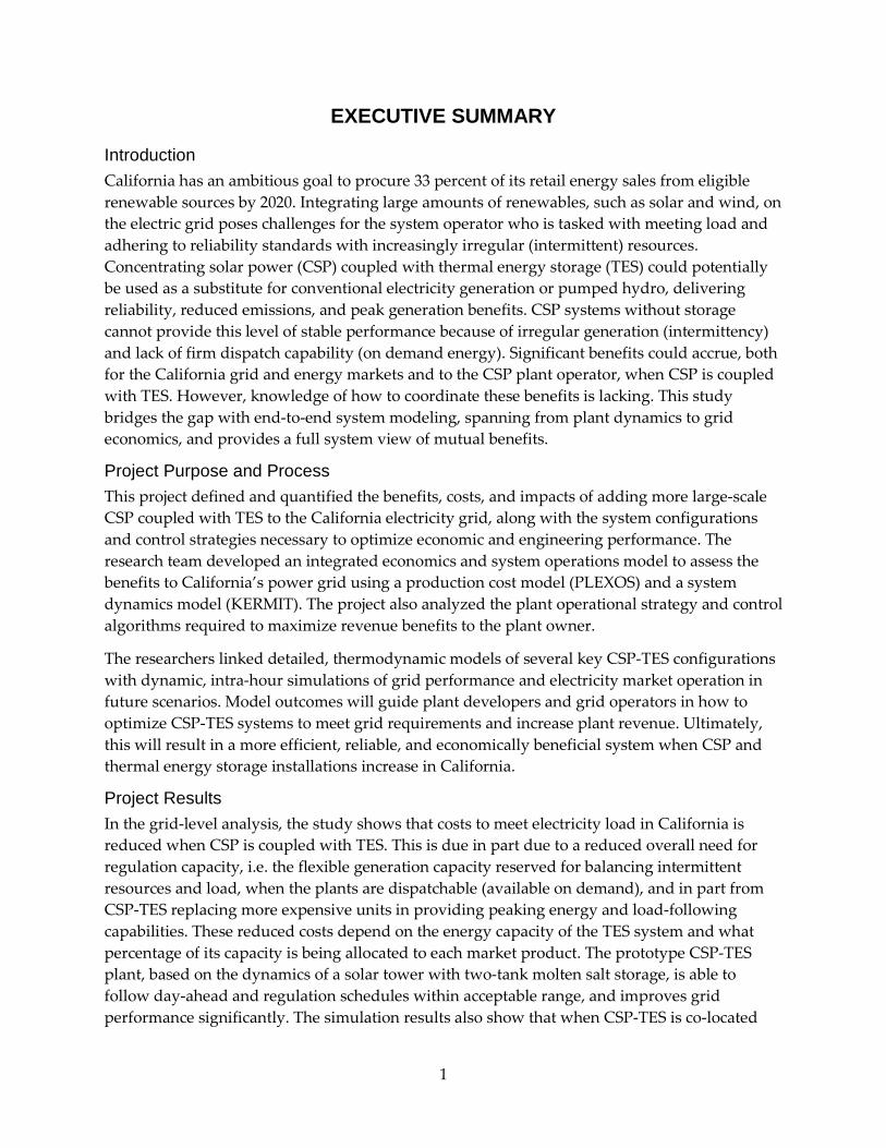
Introduction California has an ambitious goal to procure 33 percent of its retail energy sales from eligible renewable sources by 2020. Integrating large amounts of renewables, such as solar and wind, on the electric grid poses challenges for the system operator who is tasked with meeting load and adhering to reliability standards with increasingly irregular (intermittent) resources. Concentrating solar power (CSP) coupled with thermal energy storage (TES) could potentially be used as a substitute for conventional electricity generation or pumped hydro, delivering reliability, reduced emissions, and peak generation benefits. CSP systems without storage cannot provide this level of stable performance because of irregular generation (intermittency) and lack of firm dispatch capability (on demand energy). Significant benefits could accrue, both for the California grid and energy markets and to the CSP plant operator, when CSP is coupled with TES. However, knowledge of how to coordinate these benefits is lacking. This study bridges the gap with end-to-end system modeling, spanning from plant dynamics to grid economics, and provides a full system view of mutual benefits.
Project Purpose and Process This project defined and quantified the benefits, costs, and impacts of adding more large-scale CSP coupled with TES to the California electricity grid, along with the system configurations and control strategies necessary to optimize economic and engineering performance. The research team developed an integrated economics and system operations model to assess the benefits to California’s power grid using a production cost model (PLEXOS) and a system dynamics model (KERMIT). The project also analyzed the plant operational strategy and control algorithms required to maximize revenue benefits to the plant owner.
The researchers linked detailed, thermodynamic models of several key CSP-TES configurations with dynamic, intra-hour simulations of grid performance and electricity market operation in future scenarios. Model outcomes will guide plant developers and grid operators in how to optimize CSP-TES systems to meet grid requirements and increase plant revenue. Ultimately, this will result in a more efficient, reliable, and economically beneficial system when CSP and thermal energy storage installations increase in California.
Project Results In the grid-level analysis, the study shows that costs to meet electricity load in California is reduced when CSP is coupled with TES. This is due in part due to a reduced overall need for regulation capacity, i.e. the flexible generation capacity reserved for balancing intermittent resources and load, when the plants are dispatchable (available on demand), and in part from CSP-TES replacing more expensive units in providing peaking energy and load-following capabilities. These reduced costs depend on the energy capacity of the TES system and what percentage of its capacity is being allocated to each market product. The prototype CSP-TES plant, based on the dynamics of a solar tower with two-tank molten salt storage, is able to follow day-ahead and regulation schedules within acceptable range, and improves grid performance significantly. The simulation results also show that when CSP-TES is co-located
1
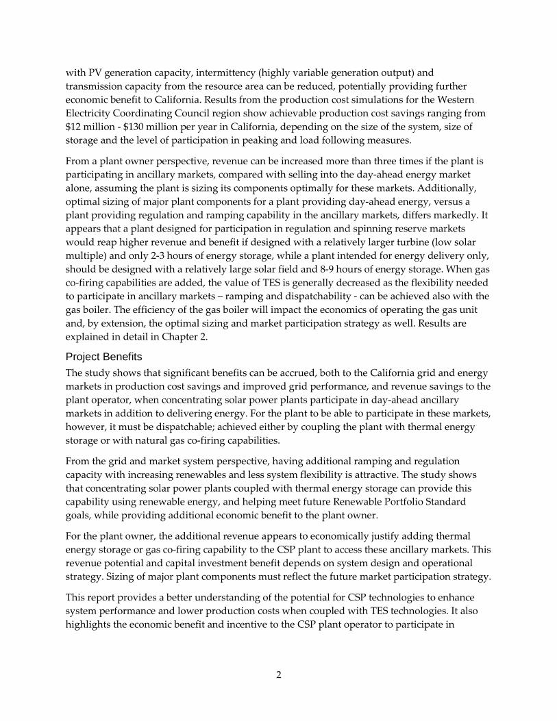
with PV generation capacity, intermittency (highly variable generation output) and transmission capacity from the resource area can be reduced, potentially providing further economic benefit to California. Results from the production cost simulations for the Western Electricity Coordinating Council region show achievable production cost savings ranging from $12 million - $130 million per year in California, depending on the size of the system, size of storage and the level of participation in peaking and load following measures.
From a plant owner perspective, revenue can be increased more than three times if the plant is participating in ancillary markets, compared with selling into the day-ahead energy market alone, assuming the plant is sizing its components optimally for these markets. Additionally, optimal sizing of major plant components for a plant providing day-ahead energy, versus a plant providing regulation and ramping capability in the ancillary markets, differs markedly. It appears that a plant designed for participation in regulation and spinning reserve markets would reap higher revenue and benefit if designed with a relatively larger turbine (low solar multiple) and only 2-3 hours of energy storage, while a plant intended for energy delivery only, should be designed with a relatively large solar field and 8-9 hours of energy storage. When gas co-firing capabilities are added, the value of TES is generally decreased as the flexibility needed to participate in ancillary markets – ramping and dispatchability - can be achieved also with the gas boiler. The efficiency of the gas boiler will impact the economics of operating the gas unit and, by extension, the optimal sizing and market participation strategy as well. Results are explained in detail in Chapter 2.
Project Benefits The study shows that significant benefits can be accrued, both to the California grid and energy markets in production cost savings and improved grid performance, and revenue savings to the plant operator, when concentrating solar power plants participate in day-ahead ancillary markets in addition to delivering energy. For the plant to be able to participate in these markets, however, it must be dispatchable; achieved either by coupling the plant with thermal energy storage or with natural gas co-firing capabilities.
From the grid and market system perspective, having additional ramping and regulation capacity with increasing renewables and less system flexibility is attractive. The study shows that concentrating solar power plants coupled with thermal energy storage can provide this capability using renewable energy, and helping meet future Renewable Portfolio Standard goals, while providing additional economic benefit to the plant owner.
For the plant owner, the additional revenue appears to economically justify adding thermal energy storage or gas co-firing capability to the CSP plant to access these ancillary markets. This revenue potential and capital investment benefit depends on system design and operational strategy. Sizing of major plant components must reflect the future market participation strategy.
This report provides a better understanding of the potential for CSP technologies to enhance system performance and lower production costs when coupled with TES technologies. It also highlights the economic benefit and incentive to the CSP plant operator to participate in
2
ancillary markets and discusses the optimal sizing of TES, the turbine and solar field to maximize this benefit.
3
CHAPTER 1: Introduction and Project Overview California has an ambitious goal to procure 33 percent of its retail energy sales from eligible renewable sources by 2020, as outlined in the state Renewable Portfolio Standard (RPS). Integrating large amounts of renewables, such as solar and wind, on the electric grid could potentially pose challenges for the system operator who is tasked with meeting load and adhering to reliability standards with increasingly intermittent resources. Concentrating Solar Power (CSP) coupled with Thermal Energy Storage (TES) (CSP-TES) may have a unique opportunity in this market context: a renewable resource that can provide firm, dispatchable energy as well as ancillary services (AS) to mitigate ramping and intermittency issues caused by other renewable generation, as well as lower the burden on conventional generation to provide ramping and reserves.
Today, only a small portion of the California energy mix is provided by CSP and impact and benefits to the grid from coupling future capacity with thermal storage are understood mainly on a qualitative level. In addition, dynamic performance of these plants, meaning, how well they are able to respond to control signals and operate in day-ahead markets for energy and ancillaries, and in extension how their performance will impact grid control, is not well understood. Further, the revenue-optimal operation and design of these future plants will depend on this performance and ability to participate in ancillary markets.
In an increasingly complex energy market and grid operations environment, quantifying the economic and operational benefits to the electricity grid, as well as identifying the design implications and revenue potential for the plant owner, are complex tasks involving dynamic performance modeling at an intra-hour timeframe for the entire grid system as well as for the detailed plant model, and includes modeling of market operations, energy, and fuel prices in future scenarios. For renewable production, annual forecasts are needed as well as the impact of forecast error. However, understanding the true value, capability, and impact of the technology is paramount for making long-term investment decisions on the one hand, and plan for future generation portfolio management on the other hand. This study is intended to bridge the gap with end-to-end system modeling, spanning from plant dynamics to grid economics.
To that end, the overarching goal of this project is to define the benefits, costs, and impacts of increasing penetration of coupled CSP-TES to the California electricity grid, along with the system configurations and control strategies needed to optimize economic and engineering performance. This goal will be achieved by linking detailed, thermodynamic models of several key CSP-TES configurations with dynamic, intra-hour simulations of grid performance and electricity market operation in future scenarios. Model outcomes will give plant developers guidance on how to optimize their systems to meet the needs of the grid and increase revenue, while simultaneously giving grid operators and regulators guidance on how to integrate CSP-TES into their systems. Ultimately, this will result in a more efficient, more reliable, and economically beneficial system when CSP and storage penetration increases in California.
4
1.1 System-Level versus Plant-Level Analysis of CSP-TES At a high level, the work conducted in this study examines optimal operation of the CSP-TES plant from 1) a system-level perspective, meaning the electricity grid operator, and 2) a plant-level perspective, meaning, the plant operator or investor. In both cases, economic modeling is performed for a full year with hourly granularity, reflecting a future scenario with high penetration of CSP-TES, in order to determine the optimal dispatch for reducing production cost in California on the one hand, and for maximizing plant revenue on the other hand. Linked with the economic dispatch optimization, a dynamic simulation on the intra-hour time scale is performed, in order to assess impact on grid operations and control as well as to verify the capability of CSP-TES plants to follow the optimized schedules and control signals in the regulation market.
This section summarizes the technical work performed in this study.
Grid Economics and Electricity Market Context 1.1.1The purpose of this task is to define the economic and operational context for the system modeling and define viable optimization criteria that incorporate economic behavior of the California market and multiple operational scenarios. This involves defining future scenarios, including load and generation portfolio, energy and fuel prices and renewable generation portfolio and production, as well as identifying markets and revenue streams available to the CSP-TES plant and the rules for participating in these markets. The context and requirements identified will inform the subsequent modeling tasks and is described Chapter 2.
System-Level Modeling of CSP-TES and Benefits to California 1.1.2The first phase of the project analyzes system-level benefits to California from high penetration of CSP coupled with TES. Benefits in reduced production cost when CSP-TES participates in day-ahead markets for energy, regulation and load-following is quantified, as well as operational benefits such as reduced ACE and reduced need for regulation capacity. The impact of forecast error and the ability of thermal storage to hedge against this uncertainty are also analyzed.
A prototype model of CSP-TES representing a solar tower with 2-tank molten salt thermal storage is leveraged for the analysis. This choice represents a compromise between evaluating mature older designs and new designs in the research phase. The 2-tank molten salt storage system is field-proven and appears to be state of the art in efficiency and capability. While there are arguments in favor of tower versus trough and vice versa, the technical performance of the storage system will not be different between the two. System-level analysis is done using the PLEXOS production cost modeling tool, linked with the dynamic grid simulation tool KERMIT. The methodology and results from this analysis are described in Chapter 40.
Plant-Level Design & Revenue Optimization 1.1.3The second phase of the study takes a plant-level perspective rather than a system-level view. Here, the objective is to maximize revenue for the plant-owner by participating in various electricity markets, and choosing the revenue-optimal design for these markets. A cost-benefit
5
analysis (see Chapter 6) discusses the trade-offs of various high-level design components and how this impacts the revenue potential and overall financial success of the project.
Evaluation of CSP and TES Technologies 1.1.4In conjunction with the system-level modeling and revenue optimization, the performance of specific CSP and TES technologies is analyzed. Detailed thermodynamic models are developed for selected technologies and performance is evaluated for a CSP-TES plant following set-points corresponding to the optimized dispatch schedules. The purposes of this task are to:
• Validate the system-level impact derived using the prototype model
• Validate the feasibility of schedules optimized for revenue and system-level benefit, respectively
• Uncover any performance limitations or differences between specific technologies.
6
CHAPTER 2: California Market and Operational Context System-level benefits, as well as plant-level revenue and optimal design, are highly dependent on the market and operational context. This section describes operational challenges in California associated with a future generation portfolio with high penetration of renewable generation. In addition, the markets available to CSP-TES in California are described and the potential needs in a future market are discussed.
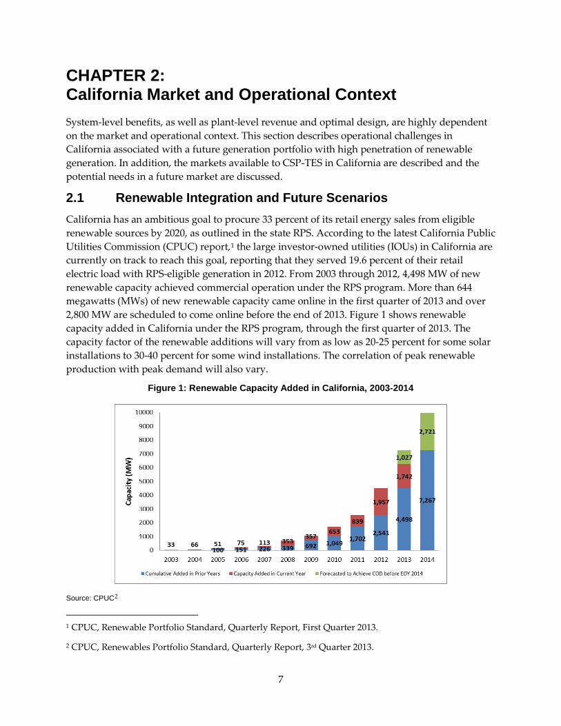
2.1 Renewable Integration and Future Scenarios California has an ambitious goal to procure 33 percent of its retail energy sales from eligible renewable sources by 2020, as outlined in the state RPS. According to the latest California Public Utilities Commission (CPUC) report,1 the large investor-owned utilities (IOUs) in California are currently on track to reach this goal, reporting that they served 19.6 percent of their retail electric load with RPS-eligible generation in 2012. From 2003 through 2012, 4,498 MW of new renewable capacity achieved commercial operation under the RPS program. More than 644 megawatts (MWs) of new renewable capacity came online in the first quarter of 2013 and over 2,800 MW are scheduled to come online before the end of 2013. Figure 1 shows renewable capacity added in California under the RPS program, through the first quarter of 2013. The capacity factor of the renewable additions will vary from as low as 20-25 percent for some solar installations to 30-40 percent for some wind installations. The correlation of peak renewable production with peak demand will also vary.
Figure 1: Renewable Capacity Added in California, 2003-2014
Source: CPUC2
1 CPUC, Renewable Portfolio Standard, Quarterly Report, First Quarter 2013.
2 CPUC, Renewables Portfolio Standard, Quarterly Report, 3rd Quarter 2013.
7
In the long-term planning process for increased renewable penetration in California, the CPUC has outlined four different RPS scenarios to be studied by the IOUs,3 each scenario achieving the 33 percent RPS goal by 2020. In addition, a 20 percent RPS reference scenario and two sensitivities around the 33 percent trajectory scenario with high and low load were required. The resulting scenarios are listed in Table 1.
Table 1: Scenarios Studied in CPUC 2010 Long-Term Procurement Proceeding
# Scenario Name Description
1 33 percent trajectory baseload Intended to model a future similar to the IOU’s current contracting and procurement activities.
2 33 percent environmentally constrained
High solar and distributed generation
3 33 percent cost constrained Focuses on resources that are lowest cost
4 33 percent time constrained Focuses on resources that can come online quickly
5 20 percent trajectory Intended to use for comparison
6 33 percent trajectory high load Reflective of future uncertainties in load growth and/or program performance
7 33 percent trajectory low load Reflective of future load uncertainties
Source: CAISO, 2011
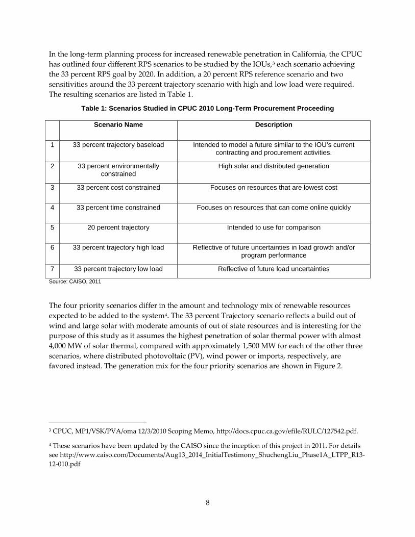
The four priority scenarios differ in the amount and technology mix of renewable resources expected to be added to the system4. The 33 percent Trajectory scenario reflects a build out of wind and large solar with moderate amounts of out of state resources and is interesting for the purpose of this study as it assumes the highest penetration of solar thermal power with almost 4,000 MW of solar thermal, compared with approximately 1,500 MW for each of the other three scenarios, where distributed photovoltaic (PV), wind power or imports, respectively, are favored instead. The generation mix for the four priority scenarios are shown in Figure 2.
3 CPUC, MP1/VSK/PVA/oma 12/3/2010 Scoping Memo, http://docs.cpuc.ca.gov/efile/RULC/127542.pdf.
4 These scenarios have been updated by the CAISO since the inception of this project in 2011. For details see http://www.caiso.com/Documents/Aug13_2014_InitialTestimony_ShuchengLiu_Phase1A_LTPP_R13-12-010.pdf
8
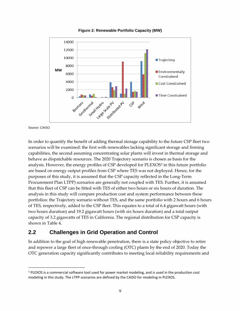
Figure 2: Renewable Portfolio Capacity (MW)
Source: CAISO
In order to quantify the benefit of adding thermal storage capability to the future CSP fleet two scenarios will be examined: the first with renewables lacking significant storage and firming capabilities, the second assuming concentrating solar plants will invest in thermal storage and behave as dispatchable resources. The 2020 Trajectory scenario is chosen as basis for the analysis. However, the energy profiles of CSP developed for PLEXOS5 in this future portfolio are based on energy output profiles from CSP where TES was not deployed. Hence, for the purposes of this study, it is assumed that the CSP capacity reflected in the Long-Term Procurement Plan LTPP) scenarios are generally not coupled with TES. Further, it is assumed that this fleet of CSP can be fitted with TES of either two hours or six hours of duration. The analysis in this study will compare production cost and system performance between these portfolios: the Trajectory scenario without TES, and the same portfolio with 2 hours and 6 hours of TES, respectively, added to the CSP fleet. This equates to a total of 6.4 gigawatt hours (with two hours duration) and 19.2 gigawatt hours (with six hours duration) and a total output capacity of 3.2 gigawatts of TES in California. The regional distribution for CSP capacity is shown in Table 4.
2.2 Challenges in Grid Operation and Control In addition to the goal of high renewable penetration, there is a state policy objective to retire and repower a large fleet of once-through cooling (OTC) plants by the end of 2020. Today the OTC generation capacity significantly contributes to meeting local reliability requirements and
5 PLEXOS is a commercial software tool used for power market modeling, and is used in the production cost modeling in this study. The LTPP scenarios are defined by the CAISO for modeling in PLEXOS.
9
at times provides as much as 80 percent of operating reserves. Figure 3 relates planned future renewable capacity additions with the OTC capacity scheduled to be retired.
Figure 3: Forecast for Flexible and Variable Capacity in California to 2020
Source: CAISO6
These two paradigm shifts happening in parallel – adding intermittent, renewable resources and replacing a large part of the load-following capacity – creates challenges for the independent system operator (ISO).
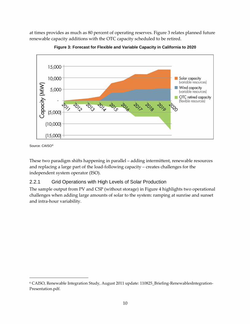
2.2.1 Grid Operations with High Levels of Solar Production The sample output from PV and CSP (without storage) in Figure 4 highlights two operational challenges when adding large amounts of solar to the system: ramping at sunrise and sunset and intra-hour variability.
6 CAISO, Renewable Integration Study, August 2011 update: 110825_Briefing-RenewablesIntegration-Presentation.pdf.
10
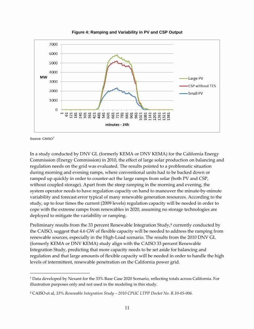
Figure 4: Ramping and Variability in PV and CSP Output
Source: CAISO7
In a study conducted by DNV GL (formerly KEMA or DNV KEMA) for the California Energy Commission (Energy Commission) in 2010, the effect of large solar production on balancing and regulation needs on the grid was evaluated. The results pointed to a problematic situation during morning and evening ramps, where conventional units had to be backed down or ramped up quickly in order to counter-act the large ramps from solar (both PV and CSP, without coupled storage). Apart from the steep ramping in the morning and evening, the system operator needs to have regulation capacity on hand to maneuver the minute-by-minute variability and forecast error typical of many renewable generation resources. According to the study, up to four times the current (2009 levels) regulation capacity will be needed in order to cope with the extreme ramps from renewables in 2020, assuming no storage technologies are deployed to mitigate the variability or ramping.
Preliminary results from the 33 percent Renewable Integration Study,8 currently conducted by the CAISO, suggest that 4.6 GW of flexible capacity will be needed to address the ramping from renewable sources, especially in the High-Load scenario. The results from the 2010 DNV GL (formerly KEMA or DNV KEMA) study align with the CAISO 33 percent Renewable Integration Study, predicting that more capacity needs to be set aside for balancing and regulation and that large amounts of flexible capacity will be needed in order to handle the high levels of intermittent, renewable penetration on the California power grid.
7 Data developed by Nexant for the 33% Base Case 2020 Scenario, reflecting totals across California. For illustration purposes only and not used in the modeling in this study.
8 CAISO et al, 33% Renewable Integration Study – 2010 CPUC LTPP Docket No. R.10-05-006.
11
2.3 Payments for CSP-TES in the California Market CSP-TES operators can sell some or all of its energy through bilateral contracts with utility or directly through CAISO’s energy markets and ancillary services market. In California, a CSP-TES typically has a Power PPA with a local utility to sell a portion or all of its energy production for a set price and a set period of time. For the remaining energy, the CSP-TES can bid into the energy or ancillary services market at the CAISO. The next few sections describe the potential revenue streams for CSP-TES in the market today as well as emerging new markets.
The system-level benefits discussed in Chapter 4 quantify benefits to California from CSP-TES participating in the Day-Ahead Energy market, Load - Following and Regulation Up and Down markets.
The design optimization analysis in Chapter 7, looking to maximize plant revenue, evaluates the CSP-TES plant participating in Day-Ahead Energy, Regulation Up and Down and Spinning Reserve Markets.
2.3.1 Contract with Utility California utilities are mandated to procure renewable energy to meet its 33 percent RPS by 2020. CSP can contract with a utility under a PPA agreement to contribute to the utility’s RPS. The average price of RPS solicitations have been below $100/MWh and expected to continue to fall. In the past few years, renewables PPAs have been dominated by PV and wind projects because of their low pricing. However, going forward, CSP-TES will have a unique value proposition to utilities due to California’s new storage procurement targets.
In October 2013, in pursuant of Assembly Bill 2514 (AB2514), the CPUC established a procurement target of 1,325 MW for the IOUs by 20209. The CPUC storage framework allocates the targets into three grid domains: transmission-connected, distributed connected and customer-side applications. Utilities must procure about half of its targets from the transmission-connected domain where CSP-TES resides. AB 2514 clearly outlines the potential impacts/benefits for energy storage in California:
"Energy storage has the potential to transform how the California electric system is conceived, designed, and operated. In so doing, energy storage has the potential to offer services needed as California seeks to maximize the value of its generation and transmission investments: optimizing the grid to avoid or defer investments in new fossil-power plants, integrating renewable power, and minimizing greenhouse emissions."
9 The research effort for this report was planned and approved to utilize the 2020 Trajectory scenario, before energy storage targets were established via Rulemaking R.10-12-007. Therefore, the analysis provided within this document does not include the incremental storage which was mandated by this bill. Additional research is recommended to assess how this additional storage might affect grid dynamics as well as pricing for ancillary services.
12
This new requirement will potentially increase the demand and price for bi-lateral contracts with CSP-TES.
2.3.2 Energy Markets – Day-Ahead and Real-Time In addition to signing a PPA with utilities, CSP-TES has the opportunity to set aside a portion or all of its capacity to participate directly in the CAISO market. In California, the CAISO operates a Day-Ahead Market and a Real-Time Market for energy. In theory, a flexible CSP-TES unit can participate in both, and in later sections the CSP-TES fleet will be modeled as participating in both Day-Ahead and Real-Time Energy market (also referred to as 5-minute dispatch or load-following) to evaluate system-level benefits.
2.3.2.1 Day-Ahead Energy Market The energy prices in the Day-Ahead Market are typically in the $20 to $40 per megawatt-hour (MWh) range. A CSP-TES plant would typically be on-line between 7 am and 8 pm so its energy price would vary between $25 and $44 per MWh (see Figure 5).
Figure 5: Average Day-Ahead Energy Prices, January – September 2011
Source: CAISO
The prices shown in Figure 5 are average locational marginal prices (LMP) in January to September 2011. The actual day to day hourly prices can vary considerably from these averages with the minimum price of -$14 to a maximum price of $121 per megawatt (MW) during this 9-month period. It is unusual to see a negative energy price in the Day-Ahead market as this means a generator is actually paying to stay on-line and generate electricity. The negative prices in this period occurred on Sunday morning on May 29 from 1 a.m. (HE2) to 8 a.m. (HE9) with the -$14 price at 6 a.m. (HE7). The assumption is that this was a very low load period, and an excess of hydro, wind, nuclear, and/or thermal generation was forced to stay on-line in spite of the negative prices in order to meet grid reliability requirements. Since a CSP-TES plant would
13
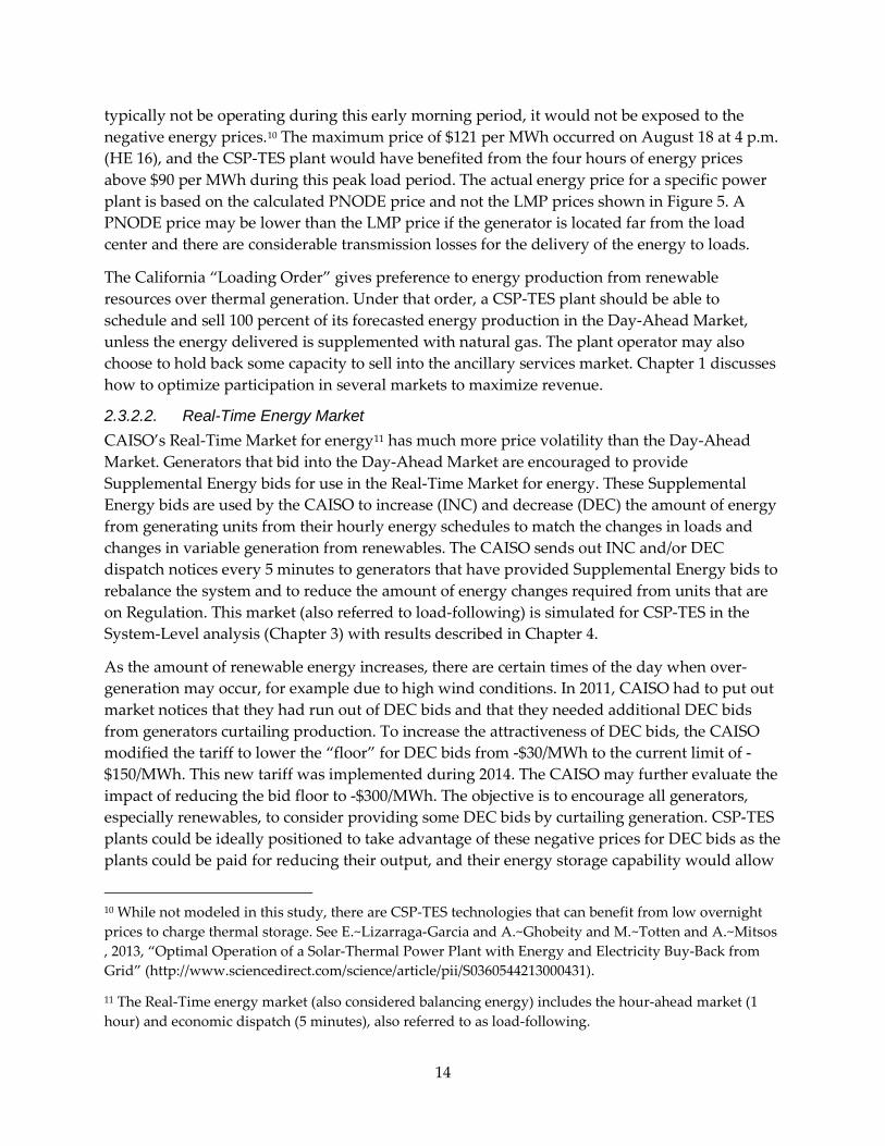
typically not be operating during this early morning period, it would not be exposed to the negative energy prices.10 The maximum price of $121 per MWh occurred on August 18 at 4 p.m. (HE 16), and the CSP-TES plant would have benefited from the four hours of energy prices above $90 per MWh during this peak load period. The actual energy price for a specific power plant is based on the calculated PNODE price and not the LMP prices shown in Figure 5. A PNODE price may be lower than the LMP price if the generator is located far from the load center and there are considerable transmission losses for the delivery of the energy to loads.
The California “Loading Order” gives preference to energy production from renewable resources over thermal generation. Under that order, a CSP-TES plant should be able to schedule and sell 100 percent of its forecasted energy production in the Day-Ahead Market, unless the energy delivered is supplemented with natural gas. The plant operator may also choose to hold back some capacity to sell into the ancillary services market. Chapter 1 discusses how to optimize participation in several markets to maximize revenue.
2.3.2.2. Real-Time Energy Market CAISO’s Real-Time Market for energy11 has much more price volatility than the Day-Ahead Market. Generators that bid into the Day-Ahead Market are encouraged to provide Supplemental Energy bids for use in the Real-Time Market for energy. These Supplemental Energy bids are used by the CAISO to increase (INC) and decrease (DEC) the amount of energy from generating units from their hourly energy schedules to match the changes in loads and changes in variable generation from renewables. The CAISO sends out INC and/or DEC dispatch notices every 5 minutes to generators that have provided Supplemental Energy bids to rebalance the system and to reduce the amount of energy changes required from units that are on Regulation. This market (also referred to load-following) is simulated for CSP-TES in the System-Level analysis (Chapter 3) with results described in Chapter 4.
As the amount of renewable energy increases, there are certain times of the day when over-generation may occur, for example due to high wind conditions. In 2011, CAISO had to put out market notices that they had run out of DEC bids and that they needed additional DEC bids from generators curtailing production. To increase the attractiveness of DEC bids, the CAISO modified the tariff to lower the “floor” for DEC bids from -$30/MWh to the current limit of -$150/MWh. This new tariff was implemented during 2014. The CAISO may further evaluate the impact of reducing the bid floor to -$300/MWh. The objective is to encourage all generators, especially renewables, to consider providing some DEC bids by curtailing generation. CSP-TES plants could be ideally positioned to take advantage of these negative prices for DEC bids as the plants could be paid for reducing their output, and their energy storage capability would allow
10 While not modeled in this study, there are CSP-TES technologies that can benefit from low overnight prices to charge thermal storage. See E.~Lizarraga-Garcia and A.~Ghobeity and M.~Totten and A.~Mitsos , 2013, “Optimal Operation of a Solar-Thermal Power Plant with Energy and Electricity Buy-Back from Grid” (http://www.sciencedirect.com/science/article/pii/S0360544213000431).
11 The Real-Time energy market (also considered balancing energy) includes the hour-ahead market (1 hour) and economic dispatch (5 minutes), also referred to as load-following.
14
them to store the reduced energy output for delivery at a later time period. The strategy would be to ensure they can bid the stored energy back into the Real-Time Markets when the energy prices are positive.
2.3.3 Ancillary Service Markets 2.3.3.1 Regulation Regulation (also called Automatic Generation Control [AGC]) consists of power output increases and decreases in response to up and down control signals. These signals are sent from a central system that senses the frequency in the grid and any variations in power flowing into and out of the control area on transmission lines (tie lines), and adjusts generator set-points to match load and restore the frequency. Currently, there is not a separate frequency regulation signal and a separate interchange error signal. The frequency error and the interchange error (actual tie-line flows – scheduled tie-line flows) are combined into an Area Control Error (ACE). The CAISO is required to keep its ACE within a tolerance band that is described in North American Electric Reliability Corporation (NERC) standards. The CAISO uses regulation and supplemental energy dispatches to control their ACE and meet the required performance standards.
The regulation market is designed to select and compensate the resources needed to provide regulation service. The CAISO typically procures 100 percent of the regulation capacity it needs in the Day-Ahead Market for each operating hour of the next day. During the real-time operating hour, the CAISO sends MW set-point commands to the units on regulation to move them up or down to new operating points to rebalance the system. The units are paid for their regulation operating range (capacity payment) and for the increase or decrease energy they provide from their hourly energy schedule. The units providing regulation do not set the real-time 5 minute energy prices but are considered price takers for the delta energy they provide.
Currently in CAISO, regulation can be scheduled and sold in each hour of the Day-Ahead Market. The regulation payment is capacity-based ($ per MW); regulating resources also receive a payment (or charge) for the net energy injected or withdrawn as a result of providing regulation service in the CAISO markets. The energy payment for regulation is based on the 5 minute Real-Time energy price.
On October 20, 2011, FERC Order 755 Frequency Regulation Compensation in the Organized Wholesale Power Markets ruled that RTOs and ISOs are required “to compensate frequency regulation resources based on the actual service provided, including a capacity payment that includes the marginal unit’s opportunity costs and a payment for performance that reflects the quantity of frequency regulation service provided by a resource when the resource is accurately following the dispatch signal.” As a result, CAISO started to implement Pay for Performance regulation in June 2013. This new payment rewards regulation resources for mileage movement between 4 second intervals as well as accuracy compared to actual telemetry.
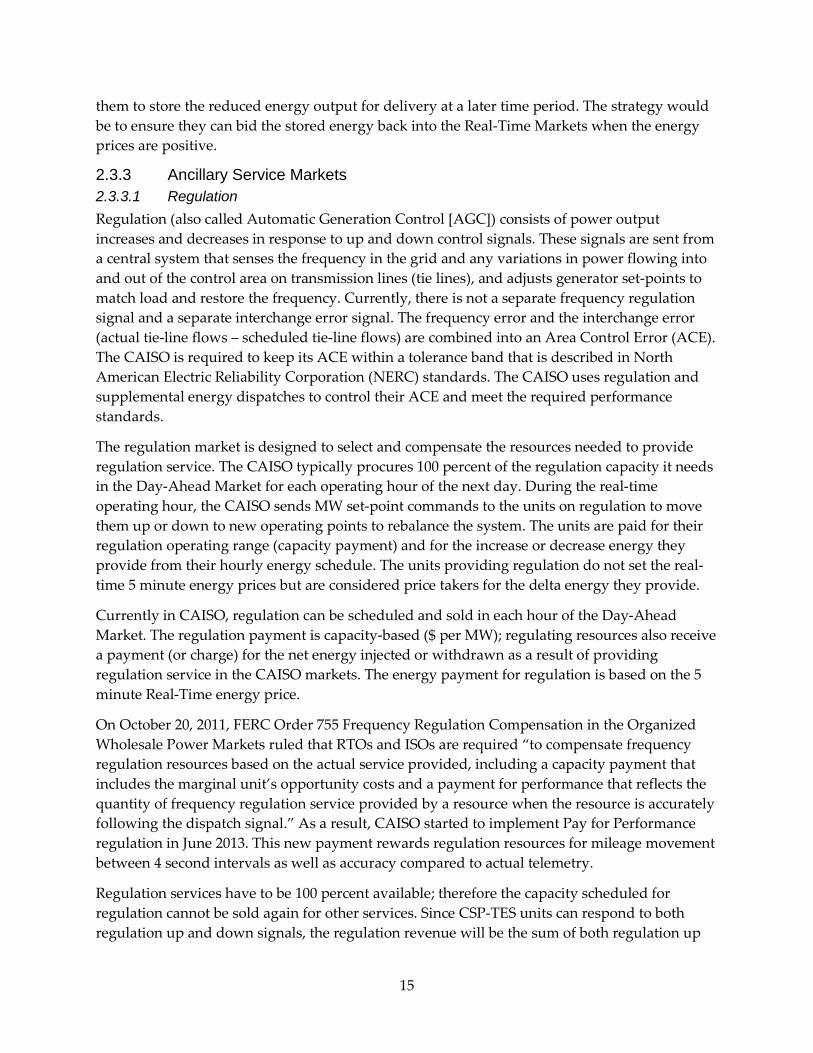
Regulation services have to be 100 percent available; therefore the capacity scheduled for regulation cannot be sold again for other services. Since CSP-TES units can respond to both regulation up and down signals, the regulation revenue will be the sum of both regulation up
15
and regulation down prices. Figure 6 shows the average regulation prices for February of 2013 to January of 2014. In these twelve months, the average regulation price ranges from $5.08 to $9.47.
Figure 6: CAISO Average Day-Ahead Regulation Prices, February 2013 – January 2014
Source: CAISO
$-
$1.00
$2.00
$3.00
$4.00
$5.00
$6.00
$7.00
$8.00
$9.00
$10.00
Feb Mar Apr May Jun Jul Aug Sep Oct Nov Dec Jan
2013 2014
RegDown
RegUp
16
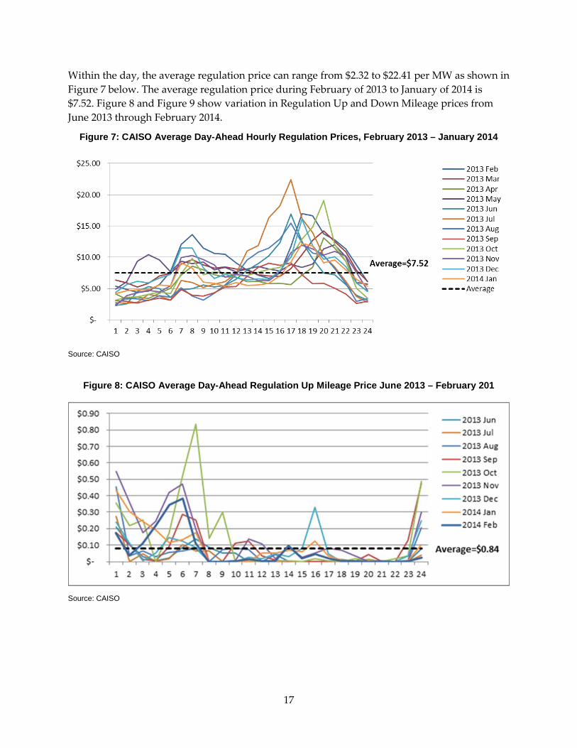
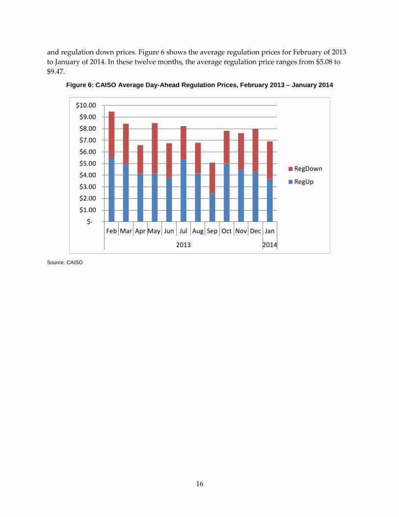
Within the day, the average regulation price can range from $2.32 to $22.41 per MW as shown in Figure 7 below. The average regulation price during February of 2013 to January of 2014 is $7.52. Figure 8 and Figure 9 show variation in Regulation Up and Down Mileage prices from June 2013 through February 2014.
Figure 7: CAISO Average Day-Ahead Hourly Regulation Prices, February 2013 – January 2014
Source: CAISO
Figure 8: CAISO Average Day-Ahead Regulation Up Mileage Price June 2013 – February 201
Source: CAISO
17
Figure 9: CAISO Average Day-Ahead Regulation Down Mileage Price, June 2013 – February 2014
Source: CAISO
2.3.3.2 Spinning and Non-Spinning Reserve Another form of ancillary services is to provide operating reserve: spinning or non-spinning. This is excess generating capacity available to a system operator to meet demand in case there is a disruption in supply. A resource providing spinning reserves is already synchronized with the grid frequency, while non-spinning reserves do not need to be synchronized but could be started up and synchronized to the grid within the allowed ramping period. In CAISO, a generator can offer unsold capacity into the day-ahead ancillary services operating reserves market and (if the offer clears the market) receive a capacity payment.
Although operating reserves are rarely called upon (typically a few times per year), when they are, they would also receive an energy payment at the market clearing price for the energy. Since the capacity payment for regulation is usually higher than that for either spinning reserves or non-spinning reserves, it is more advantageous for a CSP generator with excess capacity to bid into the regulation market (provided they have the necessary communications equipment installed and have been certified to provide this service). Figure 10 through Figure 12 show prices in the CAISO wholesale market in February 2013 through January 2014, by month and by hour, for spinning and non-spinning reserves.
18
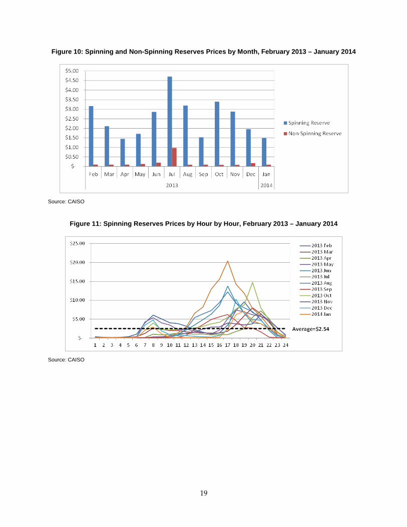
Figure 10: Spinning and Non-Spinning Reserves Prices by Month, February 2013 – January 2014
Source: CAISO
Figure 11: Spinning Reserves Prices by Hour by Hour, February 2013 – January 2014
Source: CAISO
19
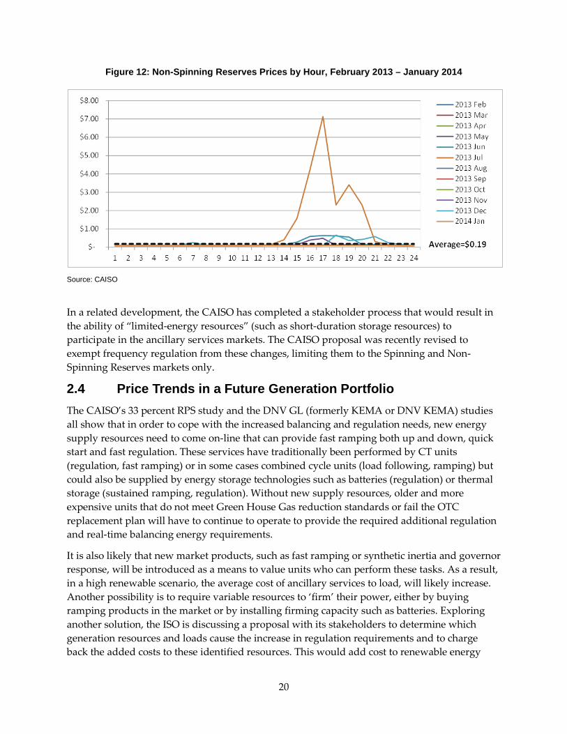
Figure 12: Non-Spinning Reserves Prices by Hour, February 2013 – January 2014
Source: CAISO
In a related development, the CAISO has completed a stakeholder process that would result in the ability of “limited-energy resources” (such as short-duration storage resources) to participate in the ancillary services markets. The CAISO proposal was recently revised to exempt frequency regulation from these changes, limiting them to the Spinning and Non-Spinning Reserves markets only.
2.4 Price Trends in a Future Generation Portfolio The CAISO’s 33 percent RPS study and the DNV GL (formerly KEMA or DNV KEMA) studies all show that in order to cope with the increased balancing and regulation needs, new energy supply resources need to come on-line that can provide fast ramping both up and down, quick start and fast regulation. These services have traditionally been performed by CT units (regulation, fast ramping) or in some cases combined cycle units (load following, ramping) but could also be supplied by energy storage technologies such as batteries (regulation) or thermal storage (sustained ramping, regulation). Without new supply resources, older and more expensive units that do not meet Green House Gas reduction standards or fail the OTC replacement plan will have to continue to operate to provide the required additional regulation and real-time balancing energy requirements.
It is also likely that new market products, such as fast ramping or synthetic inertia and governor response, will be introduced as a means to value units who can perform these tasks. As a result, in a high renewable scenario, the average cost of ancillary services to load, will likely increase. Another possibility is to require variable resources to ‘firm’ their power, either by buying ramping products in the market or by installing firming capacity such as batteries. Exploring another solution, the ISO is discussing a proposal with its stakeholders to determine which generation resources and loads cause the increase in regulation requirements and to charge back the added costs to these identified resources. This would add cost to renewable energy
20
production and, if they remain at the top of the ‘must-run’ stack, will increase the price of electricity. In extension, the following price trends can be expected:
1. Regulation: Increase in the amount of regulation required will result in an increase in regulation capacity price, especially for upward regulation. One mitigating factor for this trend may well be the development of fast and/or distributed regulation resources such as batteries, EV charging controls, electric hot water heater controls, and the like.
2. Pay for performance regulation: This new payment is mandated by FERC and will increase the total payment for regulation service.
3. Spinning reserve: Requirements for Spinning Reserve should stay the same or may actually decrease due to the increase in the amount of Regulation Up capacity that will be available in some hours as Regulation Up is also counted as Spinning Reserve. Spinning Reserve is usually only dispatched when required to cover the loss of a major generation resource or an energy import on a transmission line. If the supply of on-line dispatchable generation decreases due to the large amount of renewables on-line, then the price of Spinning Reserves and Regulation Up will both increase.
4. Non-spinning reserve: Requirements for generation that can fast start and be on-line within 10 minutes will increase as more conventional generators are forced off-line by the increase in renewable resources. Demand for non-spinning reserves may increase due to forecast errors and supply decrease because this service cannot be provided by an intermittent resource. This will likely lead to price increases.
5. Real-time (balancing) energy: The amount of real-time balancing energy required is expected to substantially increase in the future to mitigate the variability of energy supply from wind and solar renewables. Real-time price volatility and price spreads are expected to increase. Downward balancing energy is uneconomical for most renewable plants if their only option is to curtail output. It means losing the renewable tax credit for that hour and the loss of energy sale is larger than the payment for DEC bids. Consequently, the CAISO will consider lowering price floors for downward energy further, from -$150 to -$300/MWh, meaning a resource could get paid $300/MWh for reducing energy production and an energy storage and a demand response resource would be paid for consuming energy.
6. Synthetic governor response: In order to compensate conventional units, who are required to perform this governor response service, and to put a price on the cost of variability, this new market product may be introduced. However, CSP (with or without TES) would be able to provide regular governor action and system inertia.
7. Voltage support: Reactive power and voltage support is required from all conventional generators as a part of the interconnection agreements. Inverter based resources such as wind and PV solar generators are typically operated at unity power factor and do not provide voltage support. The interconnection rules and control design of these inverter based resources may have to change to insure reliable operation of the system or the
21
T&D companies will have to add substantial automatic voltage control equipment to meet voltage regulation standards.
8. Renewable energy firming requirement: Currently renewable resources can sell their power ‘as-is’ but to level the burden of variability, they may be required to compensate. This would add (explicit) cost to renewable production.
9. Flexible ramping products: Currently, the CAISO has a stakeholder initiative to design a flexible ramping product for renewable energy integration. It is an ancillary service product that aims at improving real-time market dispatch flexibility. If implemented, this will provide CSP-TES another revenue opportunity in the CAISO market. CAISO developed several draft proposals for this policy initiative in 2012 and they have scheduled to reconvene the stakeholder group in 2014.
In addition, AB2514 and Rulemaking R.10-12-007 will require the state’s 3 major utilities to implement 1.3 GW of energy storage by 2020. The legislation authorizes thermal as well as battery storage and will quickly create a market for these technologies. This will have both positive and negative impacts for TES. It could help accelerate some planned projects, but battery systems can clearly be implemented more quickly than CSP-TES. Therefore, this may present a competitive threat, and could depress regulation market pricing (in certain sectors). An alternative scenario is also possible; if large increases in solar PV installations are combined with the retirement of flexible resources, such as the once- through cooling units mentioned in Chapter 2, then the mandated supply of storage could be inadequate to accommodate the grid’s fast ramping needs. Additional analysis should be undertaken to insure these new dynamics are well understood and that the optimal regulatory resources can be provided.
For the modeling of market participation in future scenarios in this study (described in Chapter 6), hourly 2020 data for Day-Ahead Energy, Regulation Up and Down, and Spinning Reserve prices are derived from a production costing simulation of the CAISO system in PLEXOS. The simulation is based on CPUC 2010 Long Term Procurement Plan, with the 2020 Trajectory scenario assuming 4 GW of CSP-TES and with the assumption of 6 hours of thermal storage for this CSP capacity installed in the CAISO system. Average prices used are presented in Chapter 6.
2.5 System Modeling Requirements In order to optimize CSP-TES performance in a future market, a set of market rules and prices needs to be established. Market performance variables such as ramp rates, total capacity, and control logic also need to be determined. For a CSP-TES plant, a slew of operational parameters will decide which behavior is optimal in a specific market environment, including turbine capacity, captured solar heat transfer rate (area of heliostat field), power and duration of the storage facility, weather and price forecasts among other things.
From the perspective of the system operator, it is important to understand how close to the dispatch signal the plant output comes, which AGC control logic needs to be employed, and which combination of grid balancing strategies is most effective at restoring ACE and
22
frequency. Different generation portfolios will handle stresses on the grid differently, and may need to be treated differently.
2.5.1 Modeling and Optimization Criteria For a model to capture the detail in market behavior, energy balancing, plant outputs and decision making, a range of data needs to be collected that describe these behaviors, such as:
• Generation profiles for renewable resources or equivalent weather data for modeling plant output
• Regional load data, generation and imports/exports
• Market rules and pricing signals
• Transmission constraints
• Power plant dynamics and operational requirements such as capacity, ramp rates and scheduling limits
Since a lot of the grid system dynamic happens in the minute or even intra-minute time frame, second-by-second data is needed to capture this dynamic. Further, weather and load patterns change according to the season and hence data for a full year, or chosen representative days for all seasons, is required. For example, Southern California has a period known as the “June Gloom” where there is a blanket of fog or overcast sky for approximately 6 weeks which would effectively shut down all the solar PV energy production in the LA & San Diego area during many hours each day. Similarly the Sacramento valley area has 6 week heavy fog period in December and January which would shut down PV energy production in that area for an extended period. Weather patterns are a very significant variable that must be included in these models. Fortunately the weather data for areas where CSP plants will likely be installed probably does not have the same amount of variability.
When setting up a model, first one needs to establish what the model is optimizing for; it could be to maximize revenue for a specific plant, or design the best plant for taking advantage of a particular market scenario, or design the best generation portfolio to provide reliable power in all seasons or any other optimal solution to a specific question.
Second, the most significant driving factors for the subject of analysis need to be identified. Driving factors for revenue for a CSP-TES plant will include:
• Energy prices
• Operating costs (including construction)
• Plant specifications such as storage capacity and size of solar capture field
• Estimated transmission losses
• Tax credits available
• Forecast error
23
• Market rules and products available
• Level of commitment – depends on other generation available
Further, the optimized solution relates to the scenario in which it was tested. Therefore, a set of describers and variables are set to define the different scenarios, such as gas price or penetration levels of certain renewable resources. Ideally, these scenarios isolate a particular driving factor for the analysis so as to assess the impact of, say, low gas price on revenue. Scenarios that may be studied to analyze economics for a CSP-TES plant in California include:
• High and Low penetration of CSP-TES
• High and Low Energy Prices
• Tax Credits extended or terminated
• Regulation Capacity Scarce or Readily Available
2.5.2 Optimizing Plant Design and Revenue Optimizing plant design and market performance for a CSP-TES plant involves a large number of variables. A CSP-TES operating in the market would try to optimize revenue between the different services it could provide. In a study by Sioshansi and Denholm,12 the revenue of a CSP-TES in the CAISO market is optimized for different amounts of storage (0-12h), different collector field sizes, and different sets of services provided. The results show that adding energy storage to a CSP plant will increase revenue, mainly by allowing for more energy to be collected and sold and by time-shifting energy sales to peak periods. For example, a 110MW CSP plant with 6h of storage and a collector field of 2 SM13 will be able to sell energy at an average price of $67.9/MWh compared with $58.5/MWh for a plant without storage. They also show that a plant will increase its revenue with up to 11 percent if bidding up to 50 percent of its capacity into the spinning reserve market. Interestingly, the study assumes that a CSP-TES plant will not be eligible to provide regulation or non-spinning reserves due to limitations in the rate at which the power block and TES can be started and ramped. Assuming technological advancements are made, these markets should likely prove profitable to the CSP-TES plant. To compare, the present study assumes participation in the regulation and spinning reserves markets, as well as the day-ahead energy market, but not the non-spinning reserves market. These market applications and related modeling assumptions are described in Section 00.
The Sioshansi and Denholm study investigated at sensitivities around price and weather forecasting, as well as planning horizon. They found that a 24h forecast, allowing for energy to be stored overnight in order to take advantage of morning peak prices, was favorable but that a
12 IEEE, TRANSACTIONS ON SUSTAINABLE ENERGY, VOL. 1, NO. 3, OCTOBER 2010, ‘The Value of Concentrating Solar Power and Thermal Energy Storage’.
13 SM is a measurement for the size of the solar field. A solar field with an SM of one is sized to provide sufficient energy to operate the power block at its rated capacity under reference conditions. A field with an SM of two will cover twice the area of a field with an SM of one.
24
week-long planning horizon, which in theory would shift energy from weekends to weekdays, did not justify the extra storage needed. Further, the relative sizing of collector field, storage capacity and power block, will result in different market participation as the different combinations favor different behavior. As noted, ramp rates, which are tied to storage variables, storage control algorithms, heat transfer rates and choices of technology in general, will affect the capabilities and in extension the performance and optimal economic behavior for a CSP-TES unit.
As mentioned in the first section of this report, the CSP-TES plants have a unique advantage over solar PV and wind generation plants as their energy production can probably be more accurately forecasted, bid into the day-ahead energy market and include decremental bids. This would allow them to get additional payments for reducing their output when the real-time energy prices are very low or negative, yet the reduced amount of energy is not lost but simply added into the thermal storage facility, and then bid back into the real-time energy market when the price is higher. Therefore, an economic model for CSP-TES plants that takes advantage of both the energy markets and ancillary services market has greater complexity and opportunities than typical solar PV and wind generation facilities.
25
CHAPTER 3: System-Level Modeling and Benefits to the California Grid and Market The objective for this section is to quantify system-level benefits to the California electricity grid, such as production cost reductions, emissions and grid performance, due to increasing penetration of CSP coupled with TES. Based on the future scenario assumptions and markets available to CSP-TES, as described in Chapter 2, applications for CSP-TES are identified and evaluated from the perspective of the grid operator. This section describes the methodology and assumptions for modeling of CSP-TES in PLEXOS and KERMIT, aimed at quantifying these benefits. Results from this analysis are presented.
3.1 Value Proposition of CSP and TES A concentrating solar plant without thermal storage has the same advantages and challenges from the perspective of the system operator as many other renewable resources: It would count towards the RPS goal, provide a hedge against increased fuel price or fuel price volatility, but also contribute to increased forecast error and variability, hence require increased load-following and balancing capacity, as well as potentially be subject to curtailment. CSP coupled with TES, on the other hand, has the ability to provide firm energy and ancillary services and follow a day-ahead (DA) schedule, hence behave like a flexible and dispatchable, yet renewable, resource. Furthermore, while adding energy storage to other renewable sources is a possibility today, typically in the form of a battery, thermal storage is much more cost-effective for 2 hours to 12 hours of storage needed to take advantage of peak prices and act as a dispatchable resource. As such, CSP plants coupled with TES, or CSP-TES, may provide unique opportunities and benefits to the California grid compared to other intermittent resources or CSP without TES.
26
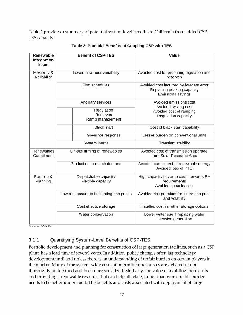
Table 2 provides a summary of potential system-level benefits to California from added CSP-TES capacity.
Table 2: Potential Benefits of Coupling CSP with TES
Renewable Integration
Issue
Benefit of CSP-TES Value
Flexibility & Reliability
Lower intra-hour variability Avoided cost for procuring regulation and reserves
Firm schedules Avoided cost incurred by forecast error Replacing peaking capacity
Emissions savings
Ancillary services Avoided emissions cost Avoided cycling cost
Avoided cost of ramping Regulation capacity
Regulation Reserves
Ramp management
Black start Cost of black start capability
Governor response Lesser burden on conventional units
System inertia Transient stability
Renewables Curtailment
On-site firming of renewables Avoided cost of transmission upgrade from Solar Resource Area
Production to match demand Avoided curtailment of renewable energy Avoided loss of PTC
Portfolio & Planning
Dispatchable capacity Flexible capacity
High capacity factor to count towards RA requirements
Avoided capacity cost
Lower exposure to fluctuating gas prices Avoided risk premium for future gas price and volatility
Cost effective storage Installed cost vs. other storage options
Water conservation Lower water use if replacing water intensive generation
Source: DNV GL
3.1.1 Quantifying System-Level Benefits of CSP-TES Portfolio development and planning for construction of large generation facilities, such as a CSP plant, has a lead time of several years. In addition, policy changes often lag technology development until and unless there is an understanding of unfair burden on certain players in the market. Many of the system-wide costs of intermittent resources are debated or not thoroughly understood and in essence socialized. Similarly, the value of avoiding these costs and providing a renewable resource that can help alleviate, rather than worsen, this burden needs to be better understood. The benefits and costs associated with deployment of large
27
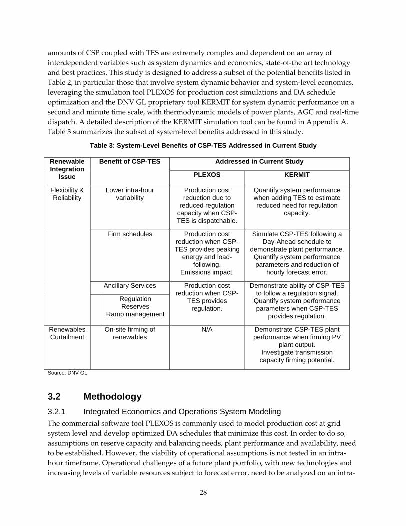
amounts of CSP coupled with TES are extremely complex and dependent on an array of interdependent variables such as system dynamics and economics, state-of-the art technology and best practices. This study is designed to address a subset of the potential benefits listed in Table 2, in particular those that involve system dynamic behavior and system-level economics, leveraging the simulation tool PLEXOS for production cost simulations and DA schedule optimization and the DNV GL proprietary tool KERMIT for system dynamic performance on a second and minute time scale, with thermodynamic models of power plants, AGC and real-time dispatch. A detailed description of the KERMIT simulation tool can be found in Appendix A. Table 3 summarizes the subset of system-level benefits addressed in this study.
Table 3: System-Level Benefits of CSP-TES Addressed in Current Study
Renewable Integration
Issue
Benefit of CSP-TES Addressed in Current Study
PLEXOS KERMIT
Flexibility & Reliability
Lower intra-hour variability
Production cost reduction due to
reduced regulation capacity when CSP-TES is dispatchable.
Quantify system performance when adding TES to estimate reduced need for regulation
capacity.
Firm schedules Production cost reduction when CSP-TES provides peaking
energy and load-following.
Emissions impact.
Simulate CSP-TES following a Day-Ahead schedule to
demonstrate plant performance. Quantify system performance parameters and reduction of
hourly forecast error.
Ancillary Services Production cost reduction when CSP-
TES provides regulation.
Demonstrate ability of CSP-TES to follow a regulation signal.
Quantify system performance parameters when CSP-TES
provides regulation.
Regulation Reserves
Ramp management
Renewables Curtailment
On-site firming of renewables
N/A Demonstrate CSP-TES plant performance when firming PV
plant output. Investigate transmission capacity firming potential.
Source: DNV GL
3.2 Methodology 3.2.1 Integrated Economics and Operations System Modeling The commercial software tool PLEXOS is commonly used to model production cost at grid system level and develop optimized DA schedules that minimize this cost. In order to do so, assumptions on reserve capacity and balancing needs, plant performance and availability, need to be established. However, the viability of operational assumptions is not tested in an intra-hour timeframe. Operational challenges of a future plant portfolio, with new technologies and increasing levels of variable resources subject to forecast error, need to be analyzed on an intra-
28
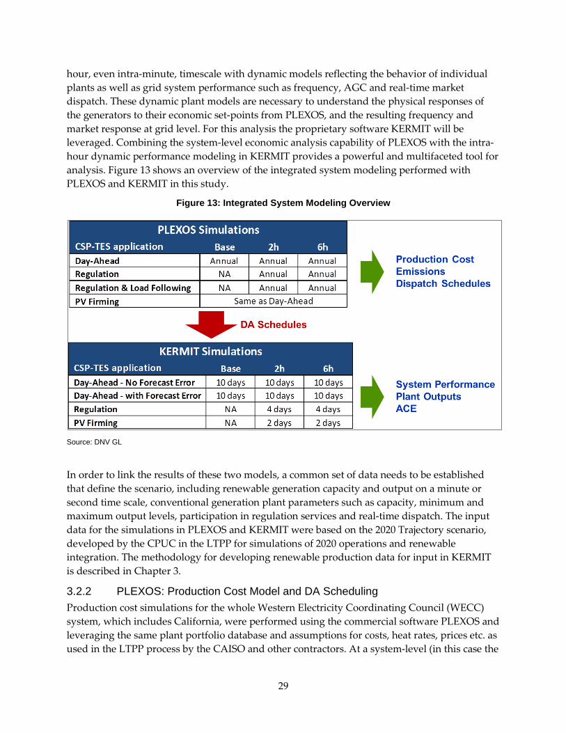
hour, even intra-minute, timescale with dynamic models reflecting the behavior of individual plants as well as grid system performance such as frequency, AGC and real-time market dispatch. These dynamic plant models are necessary to understand the physical responses of the generators to their economic set-points from PLEXOS, and the resulting frequency and market response at grid level. For this analysis the proprietary software KERMIT will be leveraged. Combining the system-level economic analysis capability of PLEXOS with the intra-hour dynamic performance modeling in KERMIT provides a powerful and multifaceted tool for analysis. Figure 13 shows an overview of the integrated system modeling performed with PLEXOS and KERMIT in this study.
Figure 13: Integrated System Modeling Overview
Source: DNV GL
In order to link the results of these two models, a common set of data needs to be established that define the scenario, including renewable generation capacity and output on a minute or second time scale, conventional generation plant parameters such as capacity, minimum and maximum output levels, participation in regulation services and real-time dispatch. The input data for the simulations in PLEXOS and KERMIT were based on the 2020 Trajectory scenario, developed by the CPUC in the LTPP for simulations of 2020 operations and renewable integration. The methodology for developing renewable production data for input in KERMIT is described in Chapter 3.
3.2.2 PLEXOS: Production Cost Model and DA Scheduling Production cost simulations for the whole Western Electricity Coordinating Council (WECC) system, which includes California, were performed using the commercial software PLEXOS and leveraging the same plant portfolio database and assumptions for costs, heat rates, prices etc. as used in the LTPP process by the CAISO and other contractors. At a system-level (in this case the
29
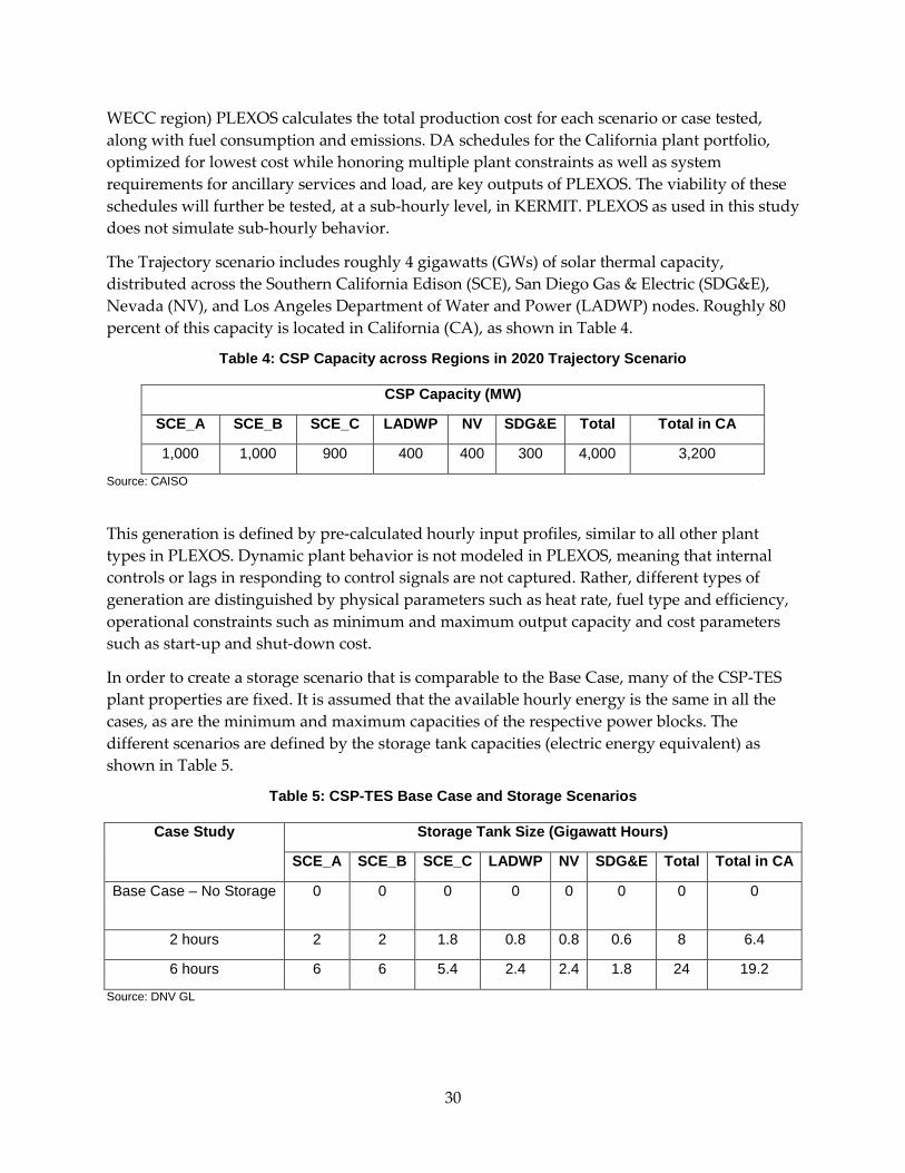
WECC region) PLEXOS calculates the total production cost for each scenario or case tested, along with fuel consumption and emissions. DA schedules for the California plant portfolio, optimized for lowest cost while honoring multiple plant constraints as well as system requirements for ancillary services and load, are key outputs of PLEXOS. The viability of these schedules will further be tested, at a sub-hourly level, in KERMIT. PLEXOS as used in this study does not simulate sub-hourly behavior.
The Trajectory scenario includes roughly 4 gigawatts (GWs) of solar thermal capacity, distributed across the Southern California Edison (SCE), San Diego Gas & Electric (SDG&E), Nevada (NV), and Los Angeles Department of Water and Power (LADWP) nodes. Roughly 80 percent of this capacity is located in California (CA), as shown in Table 4.
Table 4: CSP Capacity across Regions in 2020 Trajectory Scenario
CSP Capacity (MW)
SCE_A SCE_B SCE_C LADWP NV SDG&E Total Total in CA
1,000 1,000 900 400 400 300 4,000 3,200
Source: CAISO
This generation is defined by pre-calculated hourly input profiles, similar to all other plant types in PLEXOS. Dynamic plant behavior is not modeled in PLEXOS, meaning that internal controls or lags in responding to control signals are not captured. Rather, different types of generation are distinguished by physical parameters such as heat rate, fuel type and efficiency, operational constraints such as minimum and maximum output capacity and cost parameters such as start-up and shut-down cost.
In order to create a storage scenario that is comparable to the Base Case, many of the CSP-TES plant properties are fixed. It is assumed that the available hourly energy is the same in all the cases, as are the minimum and maximum capacities of the respective power blocks. The different scenarios are defined by the storage tank capacities (electric energy equivalent) as shown in Table 5.
Table 5: CSP-TES Base Case and Storage Scenarios
Case Study Storage Tank Size (Gigawatt Hours)
SCE_A SCE_B SCE_C LADWP NV SDG&E Total Total in CA
Base Case – No Storage 0 0 0 0 0 0 0 0
2 hours 2 2 1.8 0.8 0.8 0.6 8 6.4
6 hours 6 6 5.4 2.4 2.4 1.8 24 19.2
Source: DNV GL
30
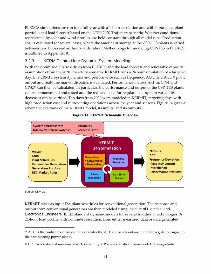
PLEXOS simulations are run for a full year with a 1-hour resolution and with input data, plant portfolio and load forecast based on the LTPP 2020 Trajectory scenario. Weather conditions, represented by solar and wind profiles, are held constant through all model runs. Production cost is calculated for several cases, where the amount of storage at the CSP-TES plants is varied between zero hours and six hours of duration. Methodology for modeling CSP-TES in PLEXOS is outlined in Appendix B.
3.2.3 KERMIT: Intra-Hour Dynamic System Modeling With the optimized DA schedules from PLEXOS and the load forecast and renewable capacity assumptions from the 2020 Trajectory scenario, KERMIT runs a 24 hour simulation of a targeted day. In KERMIT, system dynamics and performance such as frequency, AGC, and ACE,14 plant output and real-time market dispatch, is evaluated. Performance metrics such as CPS1 and CPS215 can then be calculated. In particular, the performance and output of the CSP-TES plants can be demonstrated and tested and the reduced need for regulation as system variability decreases can be verified. Ten days from 2020 were modeled in KERMIT, targeting days with high production cost and representing operations across the year and seasons. Figure 14 gives a schematic overview of the KERMIT model, its inputs, and its outputs.
Figure 14: KERMIT Schematic Overview
Source: DNV GL
KERMIT takes as input DA plant schedules for conventional generation. The response and output from conventional generators are then modeled using Institute of Electrical and Electronics Engineers (IEEE) standard dynamic models for several traditional technologies. A 24-hour load profile with 1-minute resolution, from either measured data or data generated
14 AGC is the control mechanism that calculates the ACE and sends out an automatic regulation signal to the participating power plants.
15 CPS1 is a statistical measure of ACE variability. CPS2 is a statistical measure of ACE magnitude.
31
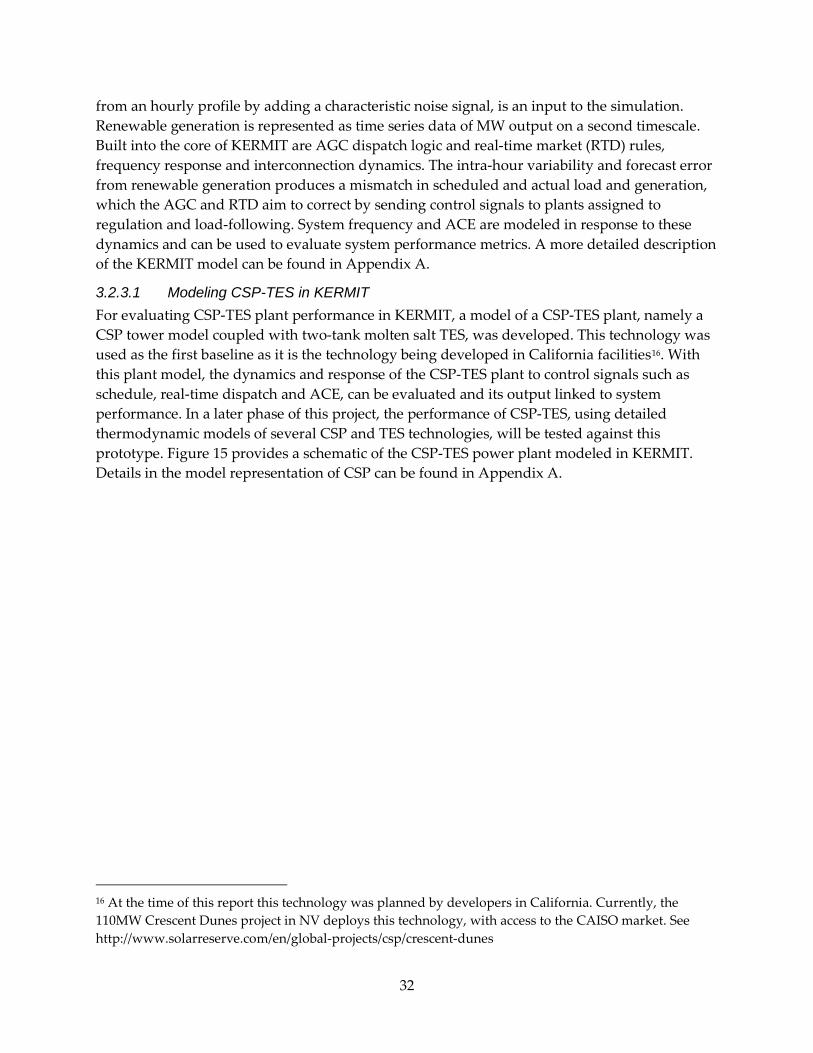
from an hourly profile by adding a characteristic noise signal, is an input to the simulation. Renewable generation is represented as time series data of MW output on a second timescale. Built into the core of KERMIT are AGC dispatch logic and real-time market (RTD) rules, frequency response and interconnection dynamics. The intra-hour variability and forecast error from renewable generation produces a mismatch in scheduled and actual load and generation, which the AGC and RTD aim to correct by sending control signals to plants assigned to regulation and load-following. System frequency and ACE are modeled in response to these dynamics and can be used to evaluate system performance metrics. A more detailed description of the KERMIT model can be found in Appendix A.
3.2.3.1 Modeling CSP-TES in KERMIT For evaluating CSP-TES plant performance in KERMIT, a model of a CSP-TES plant, namely a CSP tower model coupled with two-tank molten salt TES, was developed. This technology was used as the first baseline as it is the technology being developed in California facilities16. With this plant model, the dynamics and response of the CSP-TES plant to control signals such as schedule, real-time dispatch and ACE, can be evaluated and its output linked to system performance. In a later phase of this project, the performance of CSP-TES, using detailed thermodynamic models of several CSP and TES technologies, will be tested against this prototype. Figure 15 provides a schematic of the CSP-TES power plant modeled in KERMIT. Details in the model representation of CSP can be found in Appendix A.
16 At the time of this report this technology was planned by developers in California. Currently, the 110MW Crescent Dunes project in NV deploys this technology, with access to the CAISO market. See http://www.solarreserve.com/en/global-projects/csp/crescent-dunes
32
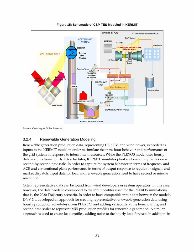
Figure 15: Schematic of CSP-TES Modeled in KERMIT
Source: Courtesy of Solar Reserve
3.2.4 Renewable Generation Modeling Renewable generation production data, representing CSP, PV, and wind power, is needed as inputs to the KERMIT model in order to simulate the intra-hour behavior and performance of the grid system in response to intermittent resources. While the PLEXOS model uses hourly data and produces hourly DA schedules, KERMIT simulates plant and system dynamics on a second-by-second timescale. In order to capture the system behavior in terms of frequency and ACE and conventional plant performance in terms of output response to regulation signals and market dispatch, input data for load and renewable generation need to have second or minute resolution.
Often, representative data can be found from wind developers or system operators. In this case however, the data needs to correspond to the input profiles used for the PLEXOS simulations, that is, the 2020 Trajectory scenario. In order to have compatible input data between the models, DNV GL developed an approach for creating representative renewable generation data using hourly production schedules (from PLEXOS) and adding variability at the hour, minute, and second time scales to represent MW production profiles for renewable generation. A similar approach is used to create load profiles, adding noise to the hourly load forecast. In addition, in
33
order to simulate the dynamics of the CSP-TES17 plant, from insolation to receiver to storage tank, heat exchanger and eventually power output, as depicted in Figure 15, the solar irradiation equivalent to the MW output represented by the Trajectory scenario was needed.
While the PLEXOS model simulates a full year with 1-hour resolution, the KERMIT model simulates 24 hours with time steps of 1 second or less. Simulation run time and data processing limitations make running more than a handful of days in KERMIT impractical. The typical approach for annualizing results from KERMIT is to simulate 6-10 selected days, chosen to represent system challenges and seasonal variation, for an understanding of how the results would translate to the full year.
A detailed description of the methodology used to create these renewable production and solar irradiation profiles, as well as the set of renewable generation and solar irradiation time series data created for the selected days, are detailed in Appendix C.
3.3 CSP-TES Applications A future CSP-TES18 fleet in California has the potential to participate in several market products and applications. The following section describes the applications, or market functions, for CSP-TES that are evaluated in this report, via simulations in PLEXOS and KERMIT. The analysis in this report aims to quantify the system-level benefits, such as enhanced grid performance and lower overall production cost to serve load in California for the applications described in this section. The analysis will also address the ability of a CSP-TES plant to perform these applications, for example, whether a CSP-TES plant is able to follow a regulation signal. This is based on the prototype CSP-TES plant implemented in KERMIT, as described in Chapter 4.
3.3.1 Base Case: No Storage In the Base Case, the CSP plants do not have coupled storage and are therefore not dispatchable. In other words, they will provide energy only when the sun is shining. Intra-hour variability is present that needs to be counter-balanced with regulation and load-following from dispatchable plants. Similarly, forecast error will be mitigated at a system-level via load-following and regulation from the dispatchable (conventional) power plant fleet. This case is the baseline for comparing cost reductions and performance metrics when adding TES to the CSP fleet and corresponds to the 2020 Trajectory scenario.
In PLEXOS, the CSP plants are modeled as firm, hourly schedules. Intra-hour variability and forecast error are not addressed. The total production cost, emissions, regulation, and load-following requirements for the system equate to the 2020 Trajectory scenario.
In KERMIT, the CSP fleet will be modeled with both intra-hour variability and forecast error with 1-second resolution, for an understanding of the impact on ACE and system performance. The CSP fleet is modeled as fixed MW output profiles, in the same fashion as other intermittent,
17 Concentrating Solar Power (CSP) coupled with Thermal Energy Storage (TES).
18 Concentrating Solar Power (CSP) coupled with Thermal Energy Storage (TES).
34
renewable generation is modeled in KERMIT, that is, without plant dynamics or ability to respond to control signals. In KERMIT, MW output profiles are typically used to model renewables since renewable plant dynamics require weather data. Weather data is typically harder to find than MW profiles based on real output data. Note that this representation of CSP, as a MW production profile, is for this stage only and intended to assess the impact of CSP on system operations without TES. For later simulations including TES, the solar radiation input to the CSP tower that would produce the baseline profile is calculated and the CSP plant dynamics are simulated including TES. The conventional generation fleet will be dispatched according to the DA schedules produced by PLEXOS and provide regulation and load-following via AGC and the real-time dispatch modeled in KERMIT, in order to balance the intermittent resources.
3.3.2 Following a DA Schedule In this application, the TES coupled with the CSP units will be used to follow a DA schedule that has been co-optimized with the conventional generation fleet. When the CSP-TES plants are able to provide dispatchable energy, it is assumed production will be shifted to evening peak hours, replacing more expensive peaking units. In addition, the TES will smooth the energy output and reduce overall system variability. This in turn will reduce the regulation capacity needed and lower costs.
In PLEXOS, the charging and discharging of the TES capacity and output of the steam turbine will be optimized for lowest cost, with the hourly energy inflow kept constant from Base Case. The simulations are run for two sizes of TES, at two hours and six hours of duration and production cost for the two cases are compared with the Base Case.
In KERMIT, the full dynamic CSP-TES plant model is leveraged and will use the DA schedules from PLEXOS for the two hour and six hour case of TES respectively. Insolation to the plant model is equivalent to the energy inflow in the Base Case. System performance is compared to the Base Case and CSP-TES plant output and ability to follow the DA schedule is evaluated.
3.3.3 Regulation and Load-Following Assuming the CSP-TES units have the response dynamics needed to follow a regulation signal, the CSP-TES unit can, in addition to following a DA schedule, provide regulation. Similarly, the CSP-TES units can participate in the Real-Time Dispatch (RTD) to provide load-following. When the CSP-TES capacity is made available for regulation and load-following, it is assumed to replace more expensive units and hence reduce production cost at a system level.
PLEXOS will allocate regulation and load-following capacity to the CSP-TES fleet, co-optimized with the DA schedules.
KERMIT will send a regulation signal to the CSP-TES plants and system and plant performance is compared with the Base Case.
3.3.4 Renewable Capacity Firming In the case where a CSP-TES plant is co-located with a PV farm, it may be capable of firming capacity and smoothing variability from the PV farm, smoothing the overall energy-delivery from the resource area. This capability is tested in KERMIT only, by adding the variability and
35
forecast error for the PV farm to the control signal (set-point) for the CSP-TES unit. The potential for reducing the variability and forecast error in the combined output of the co-located CSP-TES and PV farms can then be assessed
36
CHAPTER 4: Results: System-Level Modeling and Benefits to the California Grid and Market This section presents the results from simulations in PLEXOS and KERMIT for the applications listed in Chapter 3. The production cost and emissions results are derived from the WECC grid system modeling in PLEXOS. These simulations optimize the cost to meet load with an existing fleet, in this case the fleet outlined in the CAISO LTPP Trajectory scenario, and do not optimize for plant capital cost or individual plant revenue. The PLEXOS optimization honors plant operating constraints, such as ramps rates and minimum operating levels, while also meeting the system requirements for ancillary services and reserves, in a least-cost fashion. Reductions in production cost when CSP is coupled with TES will be compared with the Base Case (no TES) for the set of applications tested.
The results from the KERMIT simulations will quantify grid system performance on the intra-hour time-scale, given the hourly dispatch schedules produced by PLEXOS. Potential issues with intermittency, system flexibility, and ramping that are not visible in the PLEXOS simulations will be discussed, and improvements when TES is added are quantified.
Lastly, the KERMIT simulations, with the detailed, dynamic CSP-TES plant model, will allow for analysis of plant performance and ability to follow the control signals for each application tested.
4.1 Base Case: No Storage For the Base Case, production cost calculated by PLEXOS was compared with similar studies for benchmarking. Note that production cost calculations do not include capital costs of power plants, rather it calculates the cost to meet load, given a plant portfolio with capacities, heat rates, start- and stop- costs, fuel prices, and other parameters defined, along with system requirements such as total load, ancillary services, and reserve capacity. Table 6 compares the Base Case production cost in the current DNV GL (formerly KEMA or DNV KEMA) study, with other recent studies in California and WECC.
37
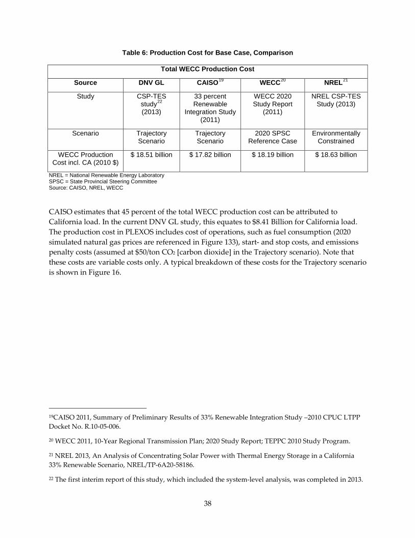
Table 6: Production Cost for Base Case, Comparison
Total WECC Production Cost
Source DNV GL CAISO19 WECC20 NREL21
Study CSP-TES study22 (2013)
33 percent Renewable
Integration Study (2011)
WECC 2020 Study Report
(2011)
NREL CSP-TES Study (2013)
Scenario Trajectory Scenario
Trajectory Scenario
2020 SPSC Reference Case
Environmentally Constrained
WECC Production Cost incl. CA (2010 $)
$ 18.51 billion $ 17.82 billion $ 18.19 billion $ 18.63 billion
NREL = National Renewable Energy Laboratory SPSC = State Provincial Steering Committee Source: CAISO, NREL, WECC
CAISO estimates that 45 percent of the total WECC production cost can be attributed to California load. In the current DNV GL study, this equates to $8.41 Billion for California load. The production cost in PLEXOS includes cost of operations, such as fuel consumption (2020 simulated natural gas prices are referenced in Figure 133), start- and stop costs, and emissions penalty costs (assumed at $50/ton CO2 [carbon dioxide] in the Trajectory scenario). Note that these costs are variable costs only. A typical breakdown of these costs for the Trajectory scenario is shown in Figure 16.
19CAISO 2011, Summary of Preliminary Results of 33% Renewable Integration Study –2010 CPUC LTPP Docket No. R.10-05-006.
20 WECC 2011, 10-Year Regional Transmission Plan; 2020 Study Report; TEPPC 2010 Study Program.
21 NREL 2013, An Analysis of Concentrating Solar Power with Thermal Energy Storage in a California 33% Renewable Scenario, NREL/TP-6A20-58186.
22 The first interim report of this study, which included the system-level analysis, was completed in 2013.
38
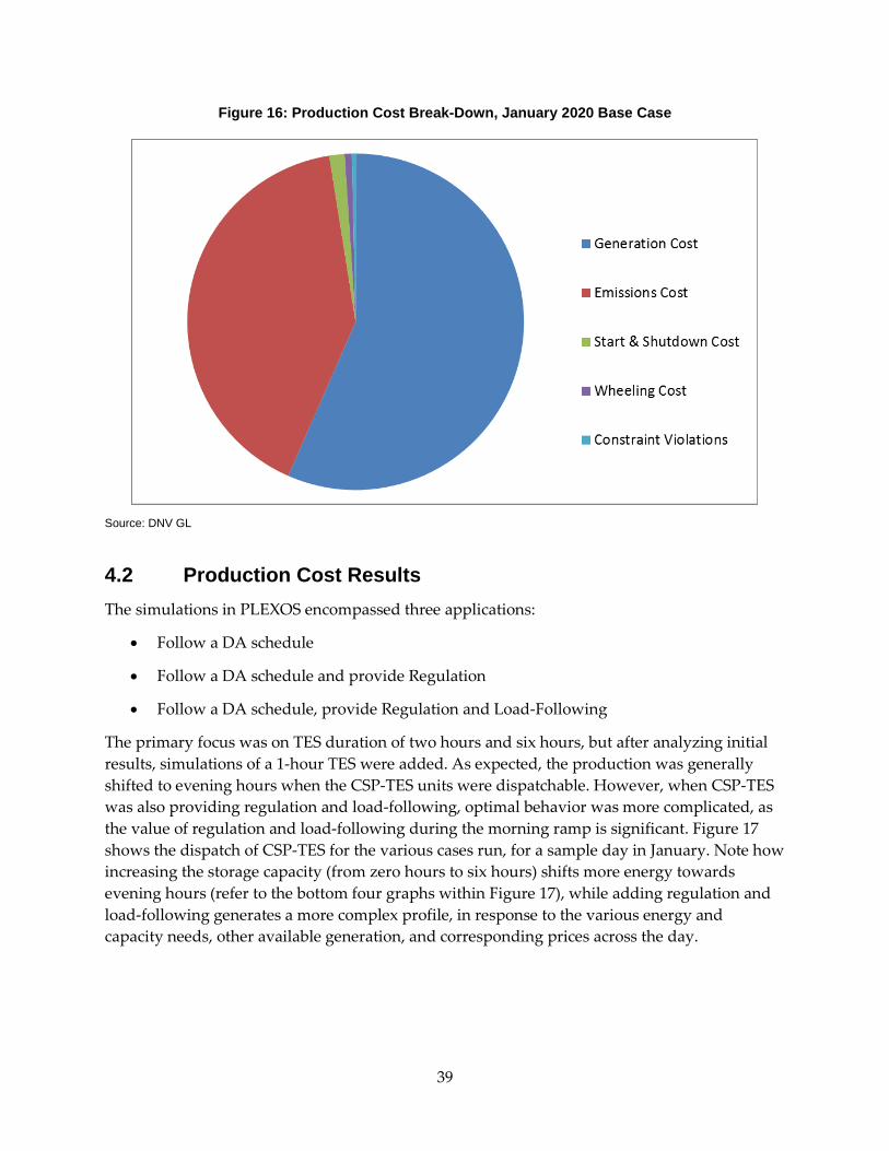
Figure 16: Production Cost Break-Down, January 2020 Base Case
Source: DNV GL
4.2 Production Cost Results The simulations in PLEXOS encompassed three applications:
• Follow a DA schedule
• Follow a DA schedule and provide Regulation
• Follow a DA schedule, provide Regulation and Load-Following
The primary focus was on TES duration of two hours and six hours, but after analyzing initial results, simulations of a 1-hour TES were added. As expected, the production was generally shifted to evening hours when the CSP-TES units were dispatchable. However, when CSP-TES was also providing regulation and load-following, optimal behavior was more complicated, as the value of regulation and load-following during the morning ramp is significant. Figure 17 shows the dispatch of CSP-TES for the various cases run, for a sample day in January. Note how increasing the storage capacity (from zero hours to six hours) shifts more energy towards evening hours (refer to the bottom four graphs within Figure 17), while adding regulation and load-following generates a more complex profile, in response to the various energy and capacity needs, other available generation, and corresponding prices across the day.
39
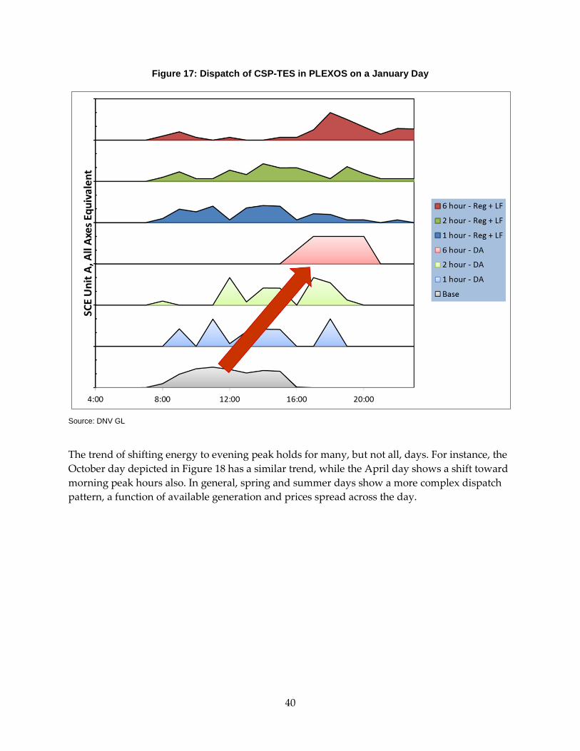
Figure 17: Dispatch of CSP-TES in PLEXOS on a January Day
Source: DNV GL
The trend of shifting energy to evening peak holds for many, but not all, days. For instance, the October day depicted in Figure 18 has a similar trend, while the April day shows a shift toward morning peak hours also. In general, spring and summer days show a more complex dispatch pattern, a function of available generation and prices spread across the day.
40
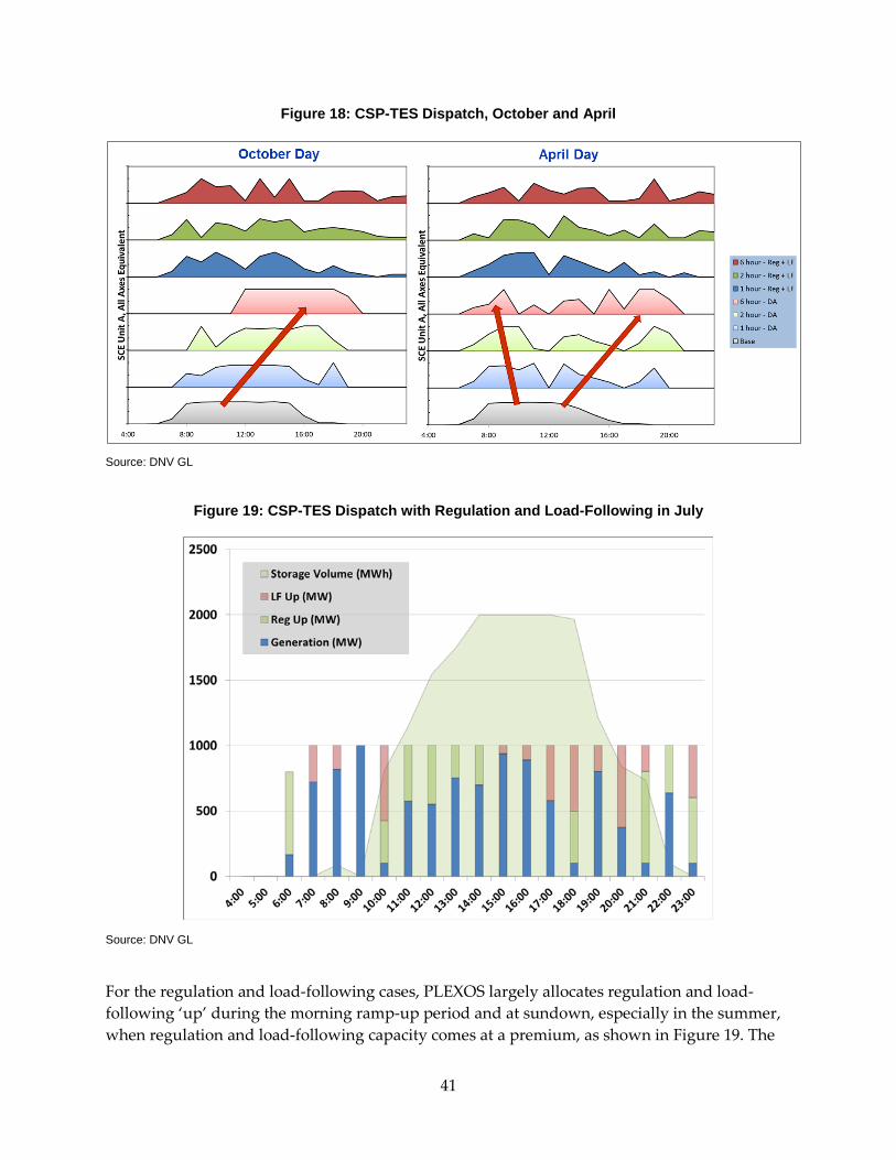
Figure 18: CSP-TES Dispatch, October and April
Source: DNV GL
Figure 19: CSP-TES Dispatch with Regulation and Load-Following in July
Source: DNV GL
For the regulation and load-following cases, PLEXOS largely allocates regulation and load-following ‘up’ during the morning ramp-up period and at sundown, especially in the summer, when regulation and load-following capacity comes at a premium, as shown in Figure 19. The
41
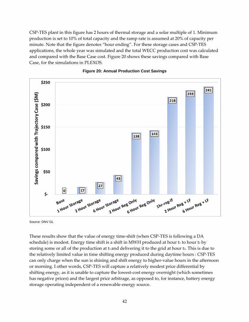
CSP-TES plant in this figure has 2 hours of thermal storage and a solar multiple of 1. Minimum production is set to 10% of total capacity and the ramp rate is assumed at 20% of capacity per minute. Note that the figure denotes “hour ending”. For these storage cases and CSP-TES applications, the whole year was simulated and the total WECC production cost was calculated and compared with the Base Case cost. Figure 20 shows these savings compared with Base Case, for the simulations in PLEXOS.
Figure 20: Annual Production Cost Savings
Source: DNV GL
These results show that the value of energy time-shift (when CSP-TES is following a DA schedule) is modest. Energy time shift is a shift in MWH produced at hour t1 to hour t2 by storing some or all of the production at t1 and delivering it to the grid at hour t2. This is due to the relatively limited value in time shifting energy produced during daytime hours : CSP-TES can only charge when the sun is shining and shift energy to higher-value hours in the afternoon or morning. I other words, CSP-TES will capture a relatively modest price differential by shifting energy, as it is unable to capture the lowest-cost energy overnight (which sometimes has negative prices) and the largest price arbitrage, as opposed to, for instance, battery energy storage operating independent of a renewable energy source.
42
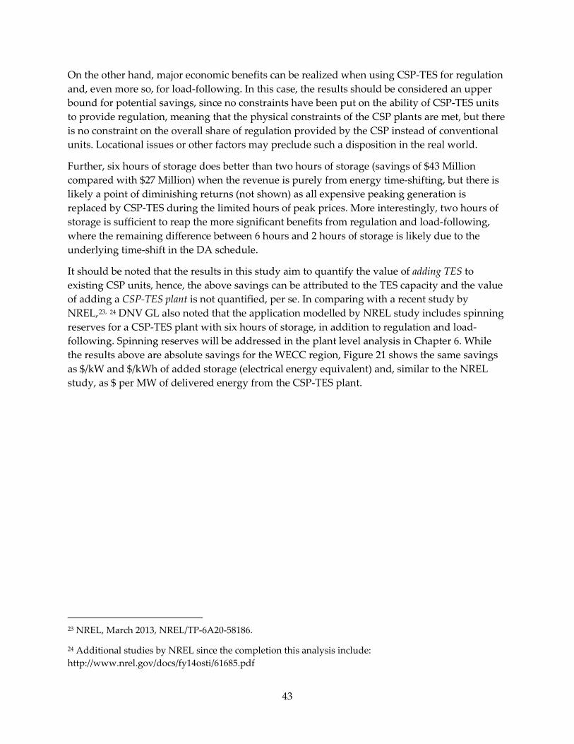
On the other hand, major economic benefits can be realized when using CSP-TES for regulation and, even more so, for load-following. In this case, the results should be considered an upper bound for potential savings, since no constraints have been put on the ability of CSP-TES units to provide regulation, meaning that the physical constraints of the CSP plants are met, but there is no constraint on the overall share of regulation provided by the CSP instead of conventional units. Locational issues or other factors may preclude such a disposition in the real world.
Further, six hours of storage does better than two hours of storage (savings of $43 Million compared with $27 Million) when the revenue is purely from energy time-shifting, but there is likely a point of diminishing returns (not shown) as all expensive peaking generation is replaced by CSP-TES during the limited hours of peak prices. More interestingly, two hours of storage is sufficient to reap the more significant benefits from regulation and load-following, where the remaining difference between 6 hours and 2 hours of storage is likely due to the underlying time-shift in the DA schedule.
It should be noted that the results in this study aim to quantify the value of adding TES to existing CSP units, hence, the above savings can be attributed to the TES capacity and the value of adding a CSP-TES plant is not quantified, per se. In comparing with a recent study by NREL,23, 24 DNV GL also noted that the application modelled by NREL study includes spinning reserves for a CSP-TES plant with six hours of storage, in addition to regulation and load-following. Spinning reserves will be addressed in the plant level analysis in Chapter 6. While the results above are absolute savings for the WECC region, Figure 21 shows the same savings as $/kW and $/kWh of added storage (electrical energy equivalent) and, similar to the NREL study, as $ per MW of delivered energy from the CSP-TES plant.
23 NREL, March 2013, NREL/TP-6A20-58186.
24 Additional studies by NREL since the completion this analysis include: http://www.nrel.gov/docs/fy14osti/61685.pdf
43
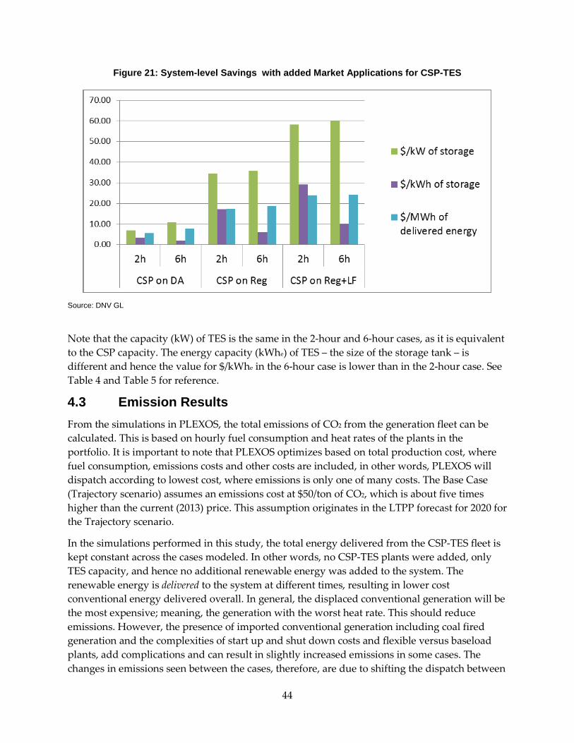
Figure 21: System-level Savings with added Market Applications for CSP-TES
Source: DNV GL
Note that the capacity (kW) of TES is the same in the 2-hour and 6-hour cases, as it is equivalent to the CSP capacity. The energy capacity (kWhe) of TES – the size of the storage tank – is different and hence the value for $/kWhe in the 6-hour case is lower than in the 2-hour case. See Table 4 and Table 5 for reference.
4.3 Emission Results From the simulations in PLEXOS, the total emissions of CO2 from the generation fleet can be calculated. This is based on hourly fuel consumption and heat rates of the plants in the portfolio. It is important to note that PLEXOS optimizes based on total production cost, where fuel consumption, emissions costs and other costs are included, in other words, PLEXOS will dispatch according to lowest cost, where emissions is only one of many costs. The Base Case (Trajectory scenario) assumes an emissions cost at $50/ton of CO2, which is about five times higher than the current (2013) price. This assumption originates in the LTPP forecast for 2020 for the Trajectory scenario.
In the simulations performed in this study, the total energy delivered from the CSP-TES fleet is kept constant across the cases modeled. In other words, no CSP-TES plants were added, only TES capacity, and hence no additional renewable energy was added to the system. The renewable energy is delivered to the system at different times, resulting in lower cost conventional energy delivered overall. In general, the displaced conventional generation will be the most expensive; meaning, the generation with the worst heat rate. This should reduce emissions. However, the presence of imported conventional generation including coal fired generation and the complexities of start up and shut down costs and flexible versus baseload plants, add complications and can result in slightly increased emissions in some cases. The changes in emissions seen between the cases, therefore, are due to shifting the dispatch between
44
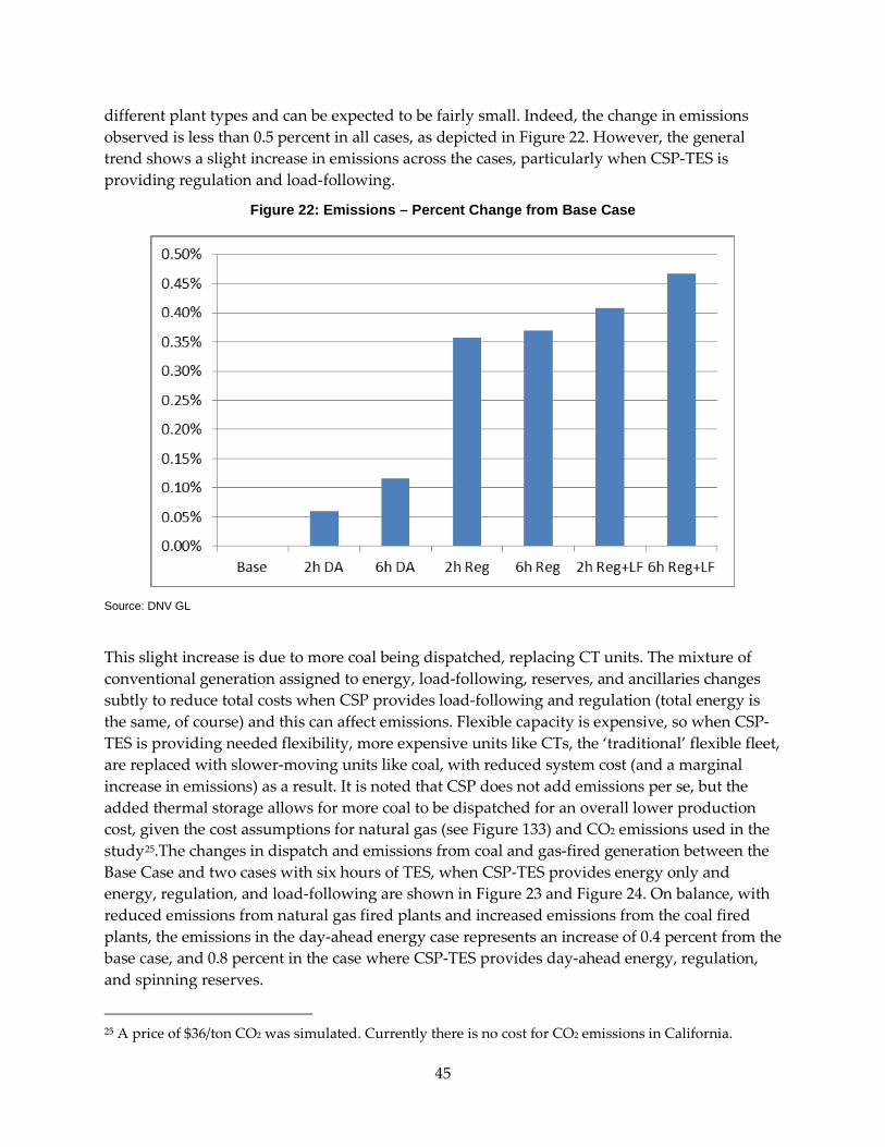
different plant types and can be expected to be fairly small. Indeed, the change in emissions observed is less than 0.5 percent in all cases, as depicted in Figure 22. However, the general trend shows a slight increase in emissions across the cases, particularly when CSP-TES is providing regulation and load-following.
Figure 22: Emissions – Percent Change from Base Case
Source: DNV GL
This slight increase is due to more coal being dispatched, replacing CT units. The mixture of conventional generation assigned to energy, load-following, reserves, and ancillaries changes subtly to reduce total costs when CSP provides load-following and regulation (total energy is the same, of course) and this can affect emissions. Flexible capacity is expensive, so when CSP-TES is providing needed flexibility, more expensive units like CTs, the ‘traditional’ flexible fleet, are replaced with slower-moving units like coal, with reduced system cost (and a marginal increase in emissions) as a result. It is noted that CSP does not add emissions per se, but the added thermal storage allows for more coal to be dispatched for an overall lower production cost, given the cost assumptions for natural gas (see Figure 133) and CO2 emissions used in the study25.The changes in dispatch and emissions from coal and gas-fired generation between the Base Case and two cases with six hours of TES, when CSP-TES provides energy only and energy, regulation, and load-following are shown in Figure 23 and Figure 24. On balance, with reduced emissions from natural gas fired plants and increased emissions from the coal fired plants, the emissions in the day-ahead energy case represents an increase of 0.4 percent from the base case, and 0.8 percent in the case where CSP-TES provides day-ahead energy, regulation, and spinning reserves.
25 A price of $36/ton CO2 was simulated. Currently there is no cost for CO2 emissions in California.
45
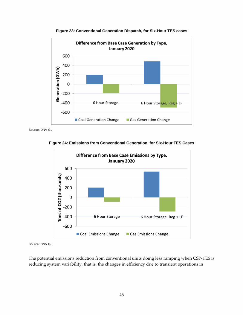
Figure 23: Conventional Generation Dispatch, for Six-Hour TES cases
Source: DNV GL
Figure 24: Emissions from Conventional Generation, for Six-Hour TES Cases
Source: DNV GL
The potential emissions reduction from conventional units doing less ramping when CSP-TES is reducing system variability, that is, the changes in efficiency due to transient operations in
46
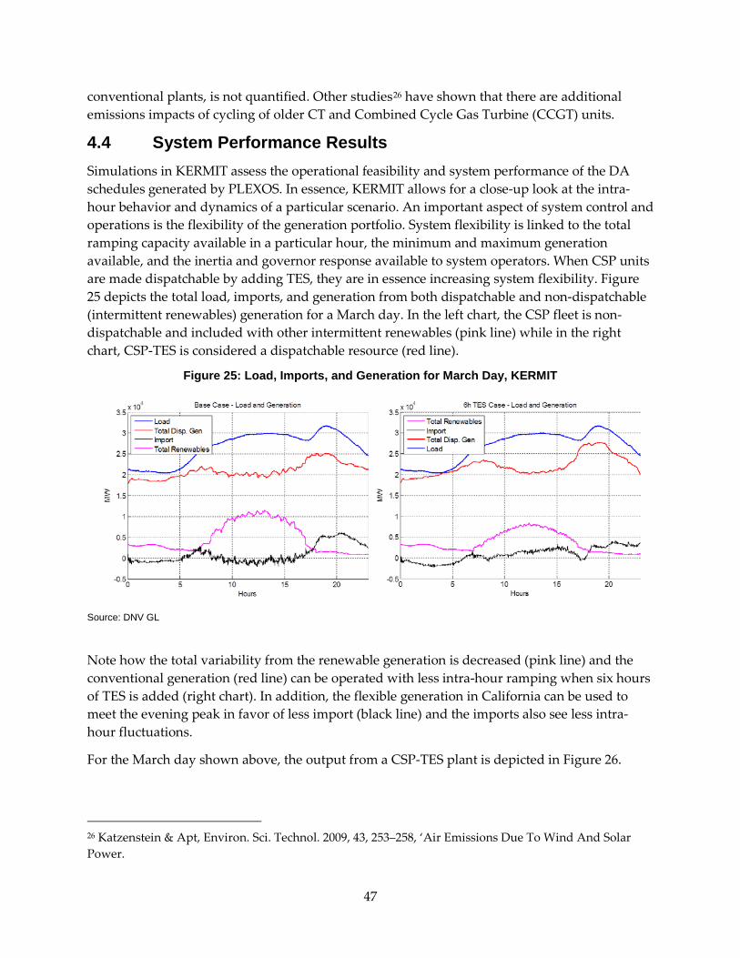
conventional plants, is not quantified. Other studies26 have shown that there are additional emissions impacts of cycling of older CT and Combined Cycle Gas Turbine (CCGT) units.
4.4 System Performance Results Simulations in KERMIT assess the operational feasibility and system performance of the DA schedules generated by PLEXOS. In essence, KERMIT allows for a close-up look at the intra-hour behavior and dynamics of a particular scenario. An important aspect of system control and operations is the flexibility of the generation portfolio. System flexibility is linked to the total ramping capacity available in a particular hour, the minimum and maximum generation available, and the inertia and governor response available to system operators. When CSP units are made dispatchable by adding TES, they are in essence increasing system flexibility. Figure 25 depicts the total load, imports, and generation from both dispatchable and non-dispatchable (intermittent renewables) generation for a March day. In the left chart, the CSP fleet is non-dispatchable and included with other intermittent renewables (pink line) while in the right chart, CSP-TES is considered a dispatchable resource (red line).
Figure 25: Load, Imports, and Generation for March Day, KERMIT
Source: DNV GL
Note how the total variability from the renewable generation is decreased (pink line) and the conventional generation (red line) can be operated with less intra-hour ramping when six hours of TES is added (right chart). In addition, the flexible generation in California can be used to meet the evening peak in favor of less import (black line) and the imports also see less intra-hour fluctuations.
For the March day shown above, the output from a CSP-TES plant is depicted in Figure 26.
26 Katzenstein & Apt, Environ. Sci. Technol. 2009, 43, 253–258, ‘Air Emissions Due To Wind And Solar Power.
47
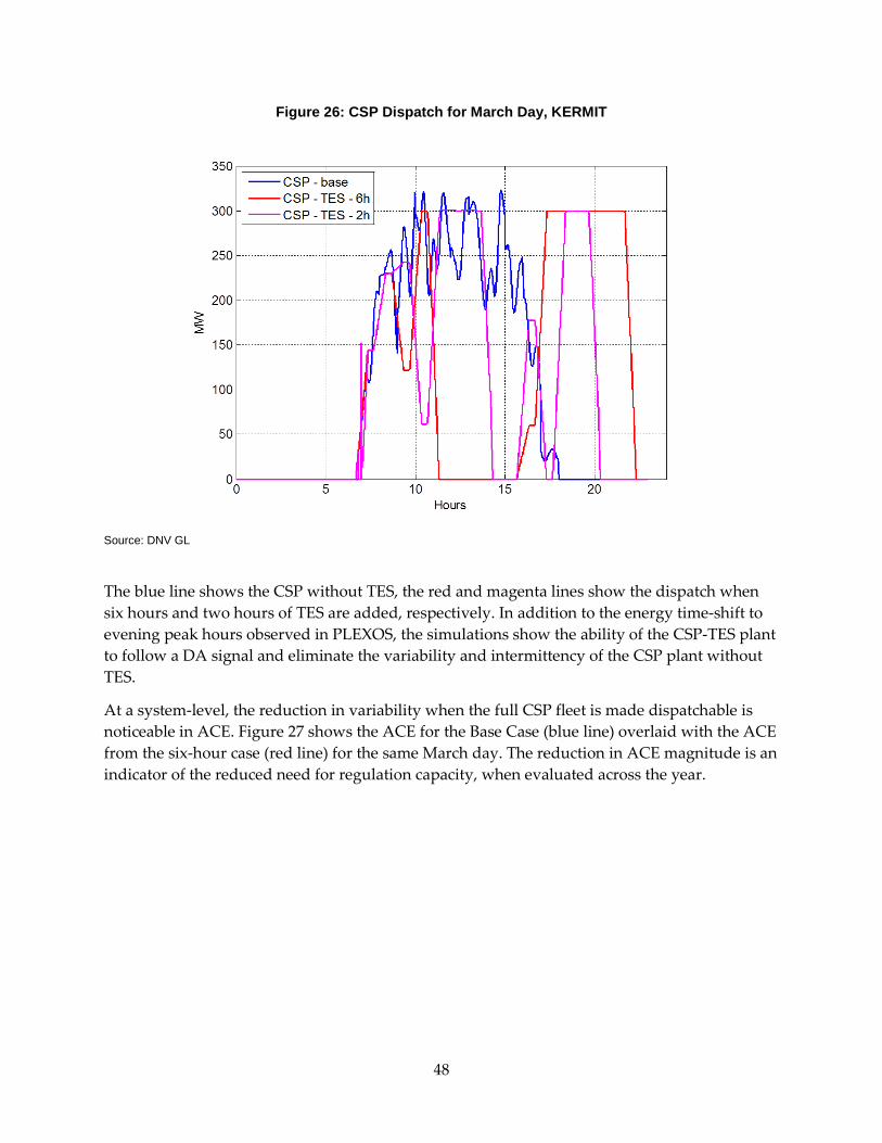
Figure 26: CSP Dispatch for March Day, KERMIT
Source: DNV GL
The blue line shows the CSP without TES, the red and magenta lines show the dispatch when six hours and two hours of TES are added, respectively. In addition to the energy time-shift to evening peak hours observed in PLEXOS, the simulations show the ability of the CSP-TES plant to follow a DA signal and eliminate the variability and intermittency of the CSP plant without TES.
At a system-level, the reduction in variability when the full CSP fleet is made dispatchable is noticeable in ACE. Figure 27 shows the ACE for the Base Case (blue line) overlaid with the ACE from the six-hour case (red line) for the same March day. The reduction in ACE magnitude is an indicator of the reduced need for regulation capacity, when evaluated across the year.
48
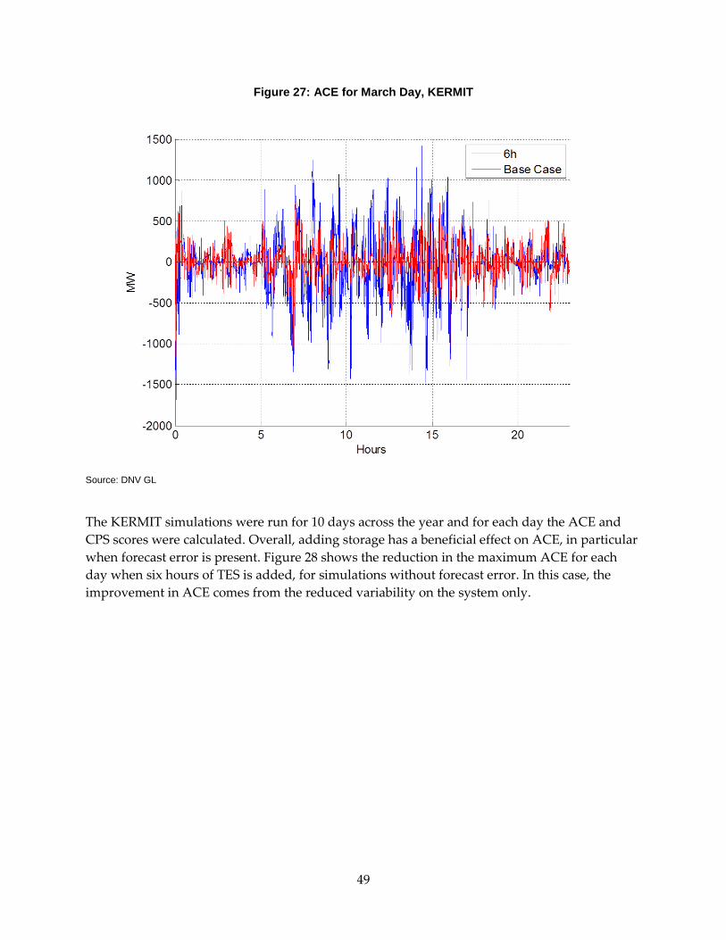
Figure 27: ACE for March Day, KERMIT
Source: DNV GL
The KERMIT simulations were run for 10 days across the year and for each day the ACE and CPS scores were calculated. Overall, adding storage has a beneficial effect on ACE, in particular when forecast error is present. Figure 28 shows the reduction in the maximum ACE for each day when six hours of TES is added, for simulations without forecast error. In this case, the improvement in ACE comes from the reduced variability on the system only.
49
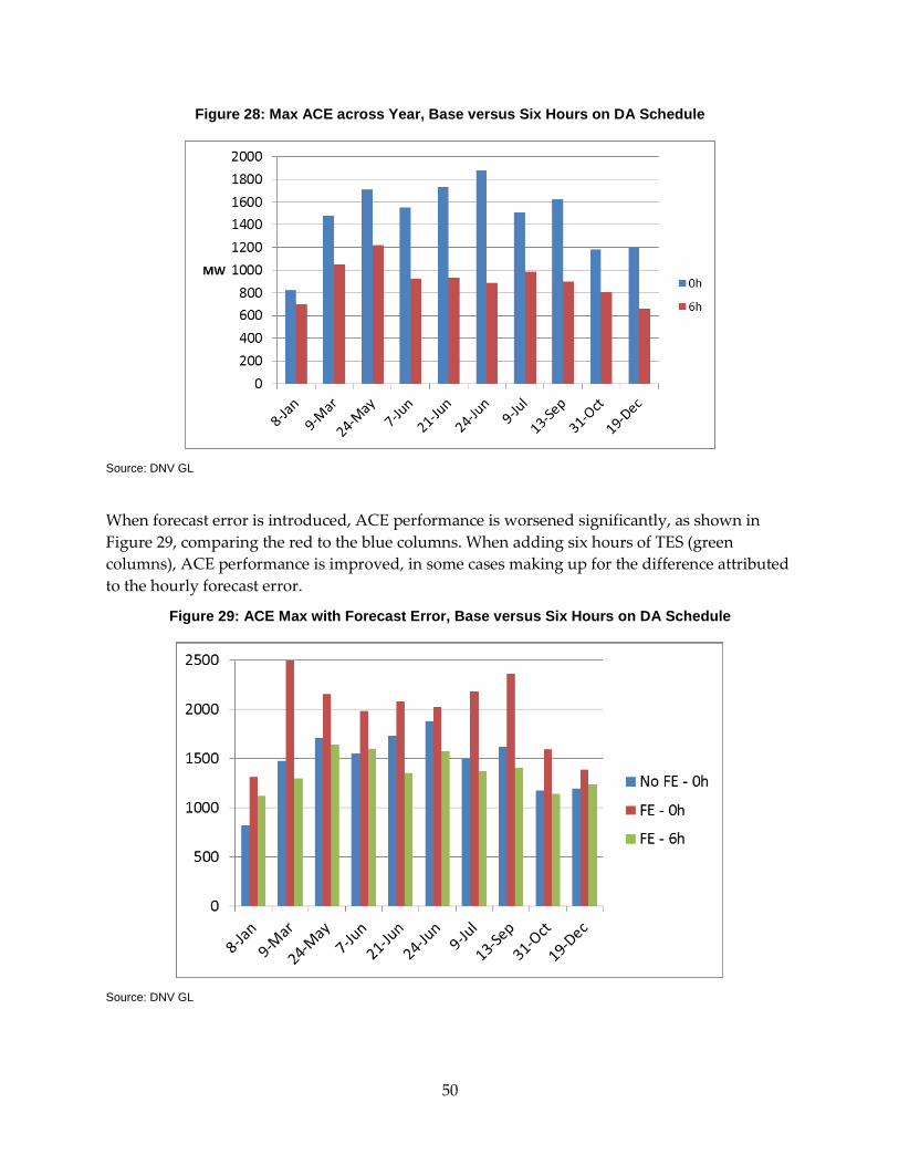
Figure 28: Max ACE across Year, Base versus Six Hours on DA Schedule
Source: DNV GL
When forecast error is introduced, ACE performance is worsened significantly, as shown in Figure 29, comparing the red to the blue columns. When adding six hours of TES (green columns), ACE performance is improved, in some cases making up for the difference attributed to the hourly forecast error.
Figure 29: ACE Max with Forecast Error, Base versus Six Hours on DA Schedule
Source: DNV GL
50
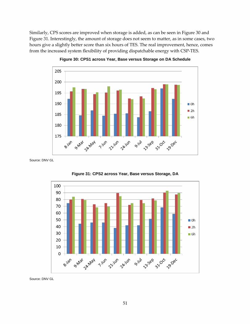
Similarly, CPS scores are improved when storage is added, as can be seen in Figure 30 and Figure 31. Interestingly, the amount of storage does not seem to matter, as in some cases, two hours give a slightly better score than six hours of TES. The real improvement, hence, comes from the increased system flexibility of providing dispatchable energy with CSP-TES.
Figure 30: CPS1 across Year, Base versus Storage on DA Schedule
Source: DNV GL
Figure 31: CPS2 across Year, Base versus Storage, DA
Source: DNV GL
51
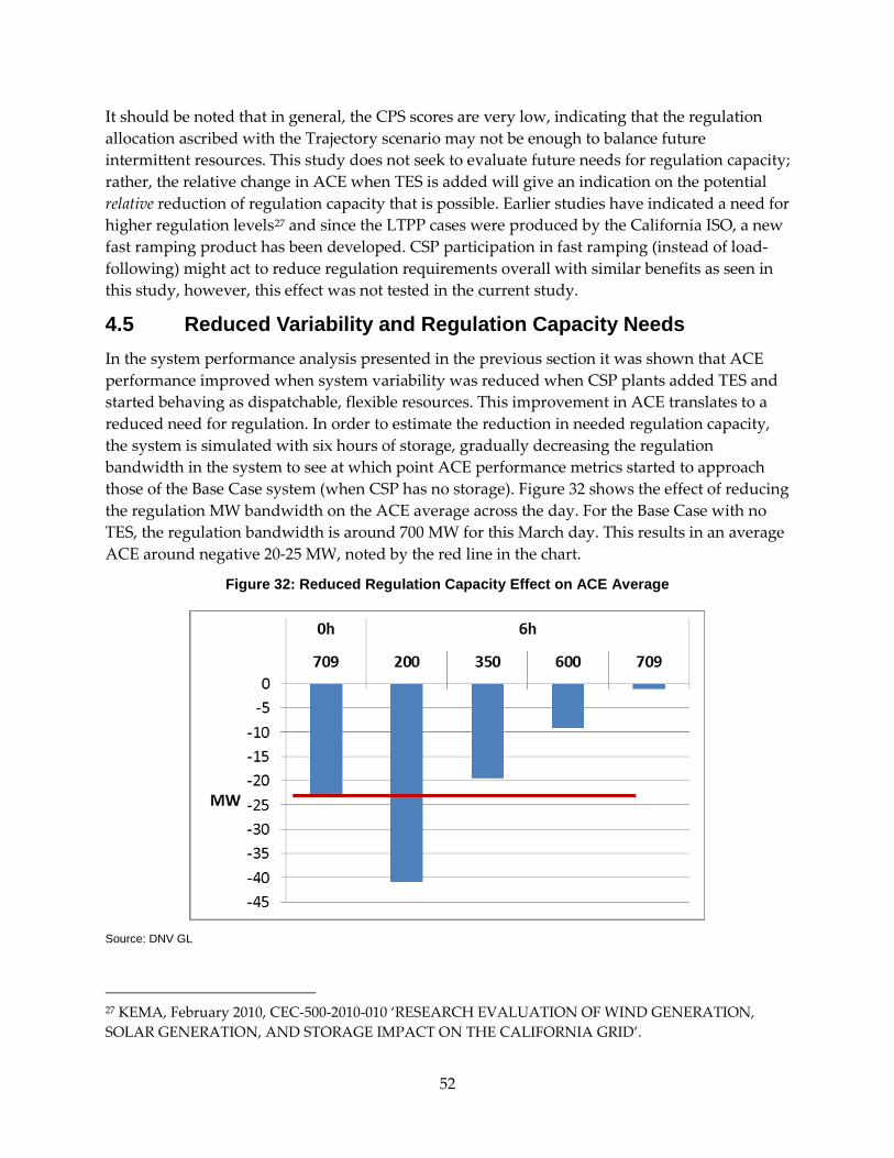
It should be noted that in general, the CPS scores are very low, indicating that the regulation allocation ascribed with the Trajectory scenario may not be enough to balance future intermittent resources. This study does not seek to evaluate future needs for regulation capacity; rather, the relative change in ACE when TES is added will give an indication on the potential relative reduction of regulation capacity that is possible. Earlier studies have indicated a need for higher regulation levels27 and since the LTPP cases were produced by the California ISO, a new fast ramping product has been developed. CSP participation in fast ramping (instead of load-following) might act to reduce regulation requirements overall with similar benefits as seen in this study, however, this effect was not tested in the current study.
4.5 Reduced Variability and Regulation Capacity Needs In the system performance analysis presented in the previous section it was shown that ACE performance improved when system variability was reduced when CSP plants added TES and started behaving as dispatchable, flexible resources. This improvement in ACE translates to a reduced need for regulation. In order to estimate the reduction in needed regulation capacity, the system is simulated with six hours of storage, gradually decreasing the regulation bandwidth in the system to see at which point ACE performance metrics started to approach those of the Base Case system (when CSP has no storage). Figure 32 shows the effect of reducing the regulation MW bandwidth on the ACE average across the day. For the Base Case with no TES, the regulation bandwidth is around 700 MW for this March day. This results in an average ACE around negative 20-25 MW, noted by the red line in the chart.
Figure 32: Reduced Regulation Capacity Effect on ACE Average
Source: DNV GL
27 KEMA, February 2010, CEC-500-2010-010 ‘RESEARCH EVALUATION OF WIND GENERATION, SOLAR GENERATION, AND STORAGE IMPACT ON THE CALIFORNIA GRID’.
52
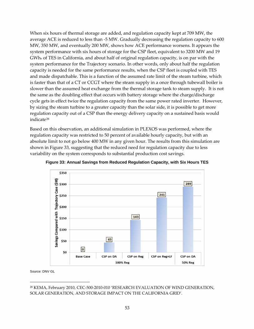
When six hours of thermal storage are added, and regulation capacity kept at 709 MW, the average ACE is reduced to less than -5 MW. Gradually decreasing the regulation capacity to 600 MW, 350 MW, and eventually 200 MW, shows how ACE performance worsens. It appears the system performance with six hours of storage for the CSP fleet, equivalent to 3200 MW and 19 GWhe of TES in California, and about half of original regulation capacity, is on par with the system performance for the Trajectory scenario. In other words, only about half the regulation capacity is needed for the same performance results, when the CSP fleet is coupled with TES and made dispatchable. This is a function of the assumed rate limit of the steam turbine, which is faster than that of a CT or CCGT where the steam supply in a once through tubewall boiler is slower than the assumed heat exchange from the thermal storage tank to steam supply. It is not the same as the doubling effect that occurs with battery storage where the charge/discharge cycle gets in effect twice the regulation capacity from the same power rated inverter. However, by sizing the steam turbine to a greater capacity than the solar side, it is possible to get more regulation capacity out of a CSP than the energy delivery capacity on a sustained basis would indicate28
Based on this observation, an additional simulation in PLEXOS was performed, where the regulation capacity was restricted to 50 percent of available hourly capacity, but with an absolute limit to not go below 400 MW in any given hour. The results from this simulation are shown in Figure 33, suggesting that the reduced need for regulation capacity due to less variability on the system corresponds to substantial production cost savings.
Figure 33: Annual Savings from Reduced Regulation Capacity, with Six Hours TES
Source: DNV GL
28 KEMA, February 2010, CEC-500-2010-010 ‘RESEARCH EVALUATION OF WIND GENERATION, SOLAR GENERATION, AND STORAGE IMPACT ON THE CALIFORNIA GRID’.
53
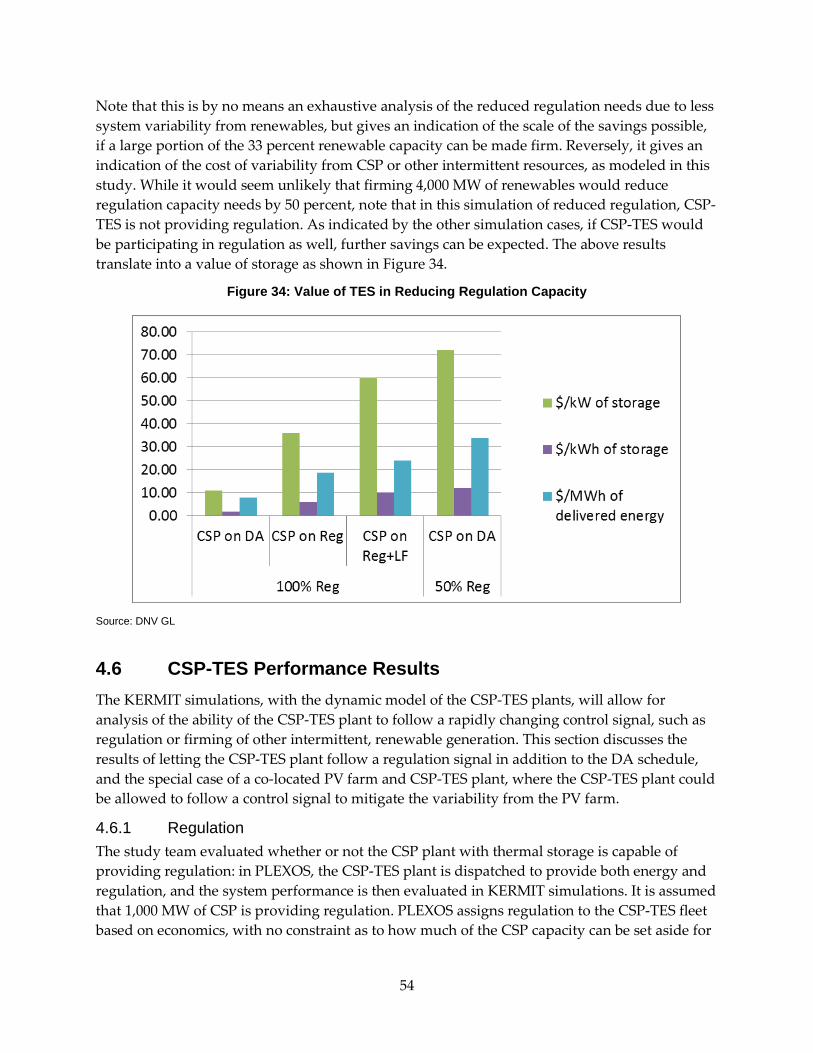
Note that this is by no means an exhaustive analysis of the reduced regulation needs due to less system variability from renewables, but gives an indication of the scale of the savings possible, if a large portion of the 33 percent renewable capacity can be made firm. Reversely, it gives an indication of the cost of variability from CSP or other intermittent resources, as modeled in this study. While it would seem unlikely that firming 4,000 MW of renewables would reduce regulation capacity needs by 50 percent, note that in this simulation of reduced regulation, CSP-TES is not providing regulation. As indicated by the other simulation cases, if CSP-TES would be participating in regulation as well, further savings can be expected. The above results translate into a value of storage as shown in Figure 34.
Figure 34: Value of TES in Reducing Regulation Capacity
Source: DNV GL
4.6 CSP-TES Performance Results The KERMIT simulations, with the dynamic model of the CSP-TES plants, will allow for analysis of the ability of the CSP-TES plant to follow a rapidly changing control signal, such as regulation or firming of other intermittent, renewable generation. This section discusses the results of letting the CSP-TES plant follow a regulation signal in addition to the DA schedule, and the special case of a co-located PV farm and CSP-TES plant, where the CSP-TES plant could be allowed to follow a control signal to mitigate the variability from the PV farm.
4.6.1 Regulation The study team evaluated whether or not the CSP plant with thermal storage is capable of providing regulation: in PLEXOS, the CSP-TES plant is dispatched to provide both energy and regulation, and the system performance is then evaluated in KERMIT simulations. It is assumed that 1,000 MW of CSP is providing regulation. PLEXOS assigns regulation to the CSP-TES fleet based on economics, with no constraint as to how much of the CSP capacity can be set aside for
54
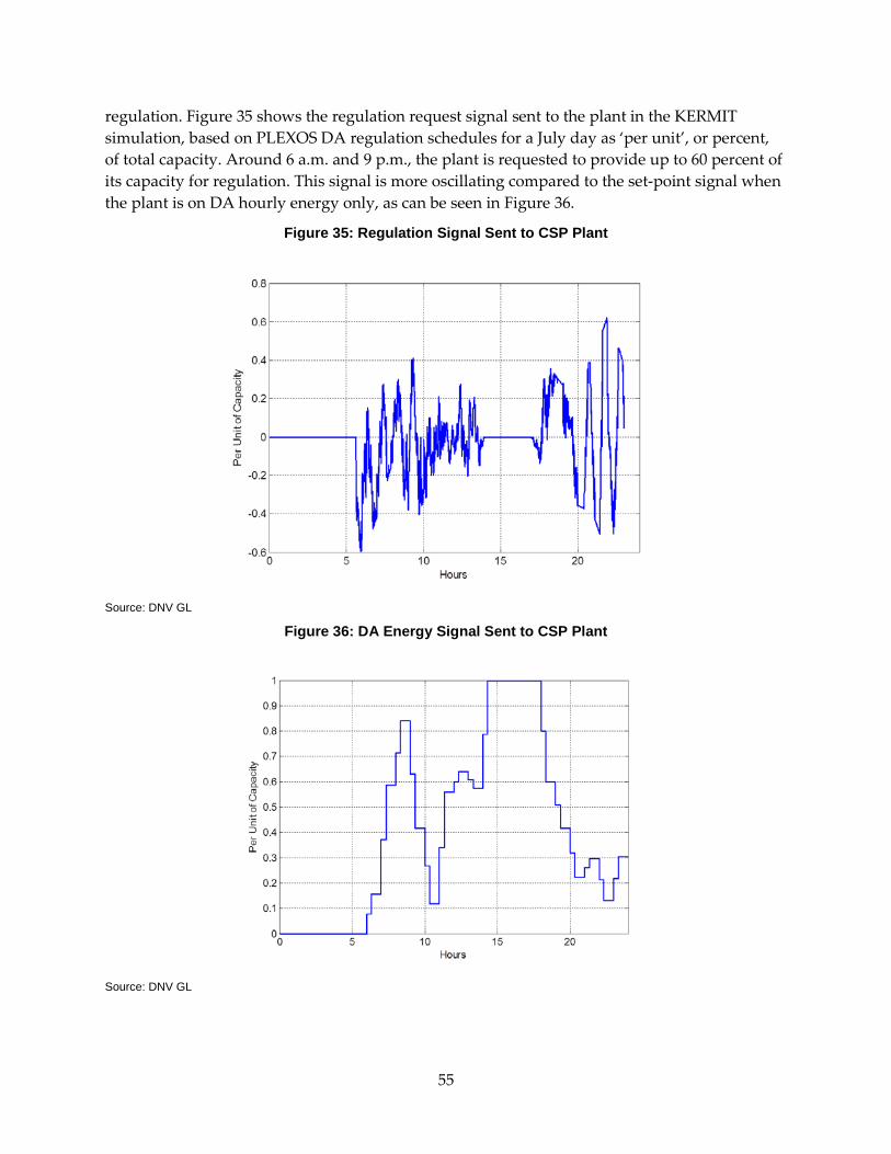
regulation. Figure 35 shows the regulation request signal sent to the plant in the KERMIT simulation, based on PLEXOS DA regulation schedules for a July day as ‘per unit’, or percent, of total capacity. Around 6 a.m. and 9 p.m., the plant is requested to provide up to 60 percent of its capacity for regulation. This signal is more oscillating compared to the set-point signal when the plant is on DA hourly energy only, as can be seen in Figure 36.
Figure 35: Regulation Signal Sent to CSP Plant
Source: DNV GL
Figure 36: DA Energy Signal Sent to CSP Plant
Source: DNV GL
55
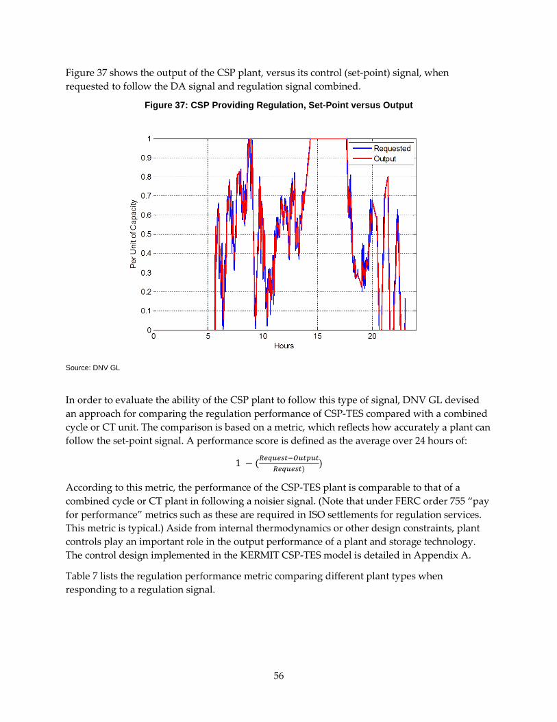
Figure 37 shows the output of the CSP plant, versus its control (set-point) signal, when requested to follow the DA signal and regulation signal combined.
Figure 37: CSP Providing Regulation, Set-Point versus Output
Source: DNV GL
In order to evaluate the ability of the CSP plant to follow this type of signal, DNV GL devised an approach for comparing the regulation performance of CSP-TES compared with a combined cycle or CT unit. The comparison is based on a metric, which reflects how accurately a plant can follow the set-point signal. A performance score is defined as the average over 24 hours of:
1 − (𝑅𝑒𝑞𝑢𝑒𝑠𝑡−𝑂𝑢𝑡𝑝𝑢𝑡𝑅𝑒𝑞𝑢𝑒𝑠𝑡)
)
According to this metric, the performance of the CSP-TES plant is comparable to that of a combined cycle or CT plant in following a noisier signal. (Note that under FERC order 755 “pay for performance” metrics such as these are required in ISO settlements for regulation services. This metric is typical.) Aside from internal thermodynamics or other design constraints, plant controls play an important role in the output performance of a plant and storage technology. The control design implemented in the KERMIT CSP-TES model is detailed in Appendix A.
Table 7 lists the regulation performance metric comparing different plant types when responding to a regulation signal.
56
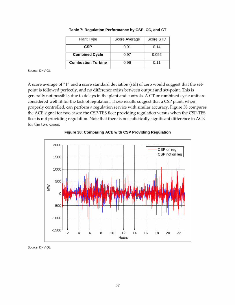
Table 7: Regulation Performance by CSP, CC, and CT
Plant Type Score Average Score STD
CSP 0.91 0.14
Combined Cycle 0.97 0.092
Combustion Turbine 0.96 0.11
Source: DNV GL
A score average of “1” and a score standard deviation (std) of zero would suggest that the set-point is followed perfectly, and no difference exists between output and set-point. This is generally not possible, due to delays in the plant and controls. A CT or combined cycle unit are considered well fit for the task of regulation. These results suggest that a CSP plant, when properly controlled, can perform a regulation service with similar accuracy. Figure 38 compares the ACE signal for two cases: the CSP-TES fleet providing regulation versus when the CSP-TES fleet is not providing regulation. Note that there is no statistically significant difference in ACE for the two cases.
Figure 38: Comparing ACE with CSP Providing Regulation
Source: DNV GL
2 4 6 8 10 12 14 16 18 20 22-1500
-1000
-500
0
500
1000
1500
2000
Hours
MW
CSP on regCSP not on reg
57
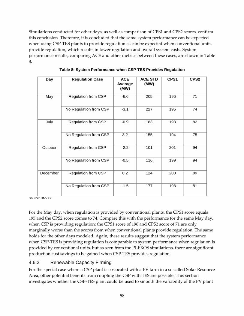
Simulations conducted for other days, as well as comparison of CPS1 and CPS2 scores, confirm this conclusion. Therefore, it is concluded that the same system performance can be expected when using CSP-TES plants to provide regulation as can be expected when conventional units provide regulation, which results in lower regulation and overall system costs. System performance results, comparing ACE and other metrics between these cases, are shown in Table 8.
Table 8: System Performance when CSP-TES Provides Regulation
Day Regulation Case ACE Average
(MW)
ACE STD (MW)
CPS1 CPS2
May Regulation from CSP -6.6 205 196 71
No Regulation from CSP -3.1 227 195 74
July Regulation from CSP -0.9 183 193 82
No Regulation from CSP 3.2 155 194 75
October Regulation from CSP -2.2 101 201 94
No Regulation from CSP -0.5 116 199 94
December Regulation from CSP 0.2 124 200 89
No Regulation from CSP -1.5 177 198 81
Source: DNV GL
For the May day, when regulation is provided by conventional plants, the CPS1 score equals 195 and the CPS2 score comes to 74. Compare this with the performance for the same May day, when CSP is providing regulation: the CPS1 score of 196 and CPS2 score of 71 are only marginally worse than the scores from when conventional plants provide regulation. The same holds for the other days modeled. Again, these results suggest that the system performance when CSP-TES is providing regulation is comparable to system performance when regulation is provided by conventional units, but as seen from the PLEXOS simulations, there are significant production cost savings to be gained when CSP-TES provides regulation.
4.6.2 Renewable Capacity Firming For the special case where a CSP plant is co-located with a PV farm in a so called Solar Resource Area, other potential benefits from coupling the CSP with TES are possible. This section investigates whether the CSP-TES plant could be used to smooth the variability of the PV plant
58
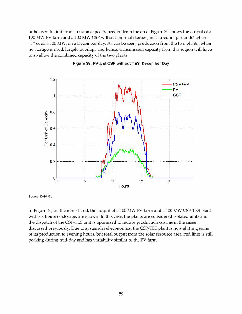
or be used to limit transmission capacity needed from the area. Figure 39 shows the output of a 100 MW PV farm and a 100 MW CSP without thermal storage, measured in ‘per units’ where “1” equals 100 MW, on a December day. As can be seen, production from the two plants, when no storage is used, largely overlaps and hence, transmission capacity from this region will have to swallow the combined capacity of the two plants.
Figure 39: PV and CSP without TES, December Day
Source: DNV GL
In Figure 40, on the other hand, the output of a 100 MW PV farm and a 100 MW CSP-TES plant with six hours of storage, are shown. In this case, the plants are considered isolated units and the dispatch of the CSP-TES unit is optimized to reduce production cost, as in the cases discussed previously. Due to system-level economics, the CSP-TES plant is now shifting some of its production to evening hours, but total output from the solar resource area (red line) is still peaking during mid-day and has variability similar to the PV farm.
59
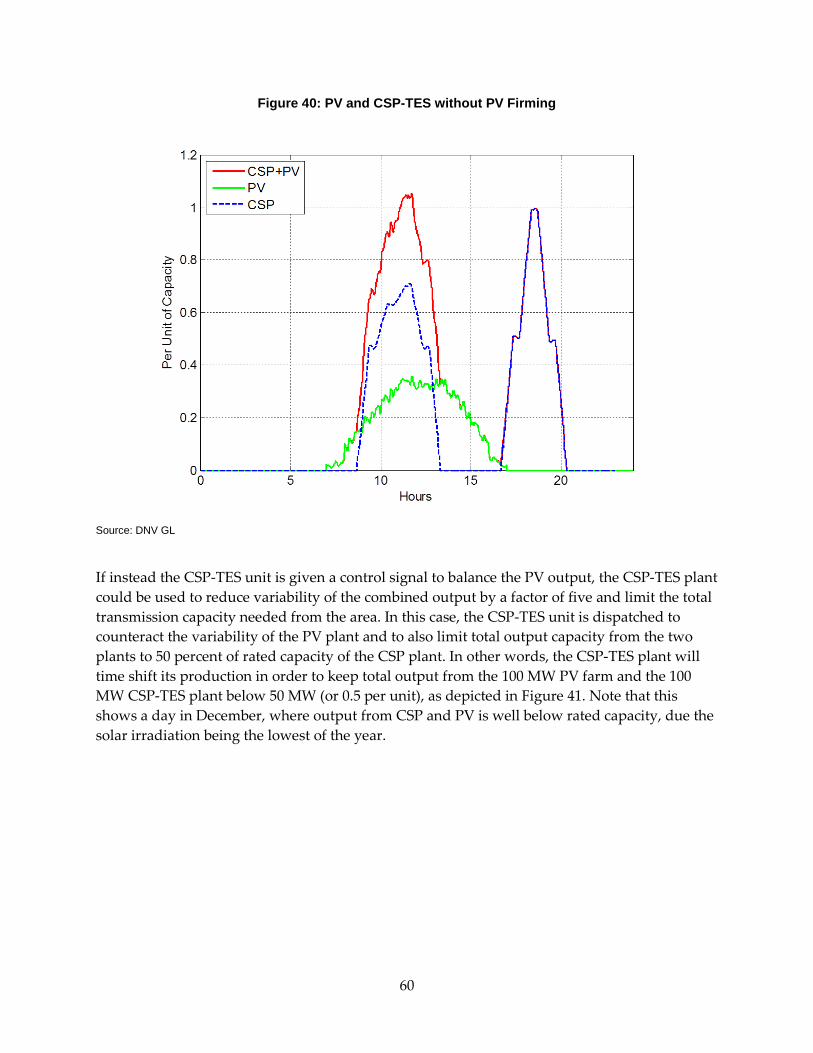
Figure 40: PV and CSP-TES without PV Firming
Source: DNV GL
If instead the CSP-TES unit is given a control signal to balance the PV output, the CSP-TES plant could be used to reduce variability of the combined output by a factor of five and limit the total transmission capacity needed from the area. In this case, the CSP-TES unit is dispatched to counteract the variability of the PV plant and to also limit total output capacity from the two plants to 50 percent of rated capacity of the CSP plant. In other words, the CSP-TES plant will time shift its production in order to keep total output from the 100 MW PV farm and the 100 MW CSP-TES plant below 50 MW (or 0.5 per unit), as depicted in Figure 41. Note that this shows a day in December, where output from CSP and PV is well below rated capacity, due the solar irradiation being the lowest of the year.
60
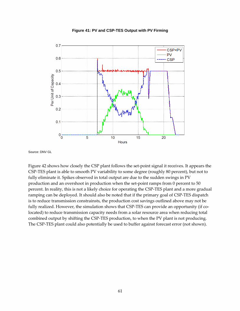
Figure 41: PV and CSP-TES Output with PV Firming
Source: DNV GL
Figure 42 shows how closely the CSP plant follows the set-point signal it receives. It appears the CSP-TES plant is able to smooth PV variability to some degree (roughly 80 percent), but not to fully eliminate it. Spikes observed in total output are due to the sudden swings in PV production and an overshoot in production when the set-point ramps from 0 percent to 50 percent. In reality, this is not a likely choice for operating the CSP-TES plant and a more gradual ramping can be deployed. It should also be noted that if the primary goal of CSP-TES dispatch is to reduce transmission constrainsts, the production cost savings outlined above may not be fully realized. However, the simulation shows that CSP-TES can provide an opportunity (if co-located) to reduce transmission capacity needs from a solar resource area when reducing total combined output by shifting the CSP-TES production, to when the PV plant is not producing. The CSP-TES plant could also potentially be used to buffer against forecast error (not shown).
61

Figure 42: CSP with Six Hour TES for PV Firming
Source: DNV GL
4.7 Summary of Results from System-Level Analysis The study methodology assumed that the CSP fleet would add TES of either two hours or six hours of duration, meaning that the storage capacity (measured in megawatt hours [MWh]) would allow the plant to produce at full capacity for the specified duration. By adding the storage capability, these renewable plants were assumed to behave like dispatchable units, capable of following a day-ahead schedule or a regulation signal. The simulations in KERMIT tested the capability of the CSP-TES plants in following the corresponding control signals, and calculated the resulting system performance metrics. Simulations in PLEXOS quantified the production cost savings for these CSP-TES applications. In addition, a situation with co-located29 PV and CSP was evaluated in order to determine the possibilities for co-optimizing the output from the two resources. The parameters quantified in the system-level analysis are listed in Table 9.
29 The case considers a situation when the two resources share a transmission line and can be co-optimized fo the transmission capacity. They do not need to connect to the same node necessarily.
62
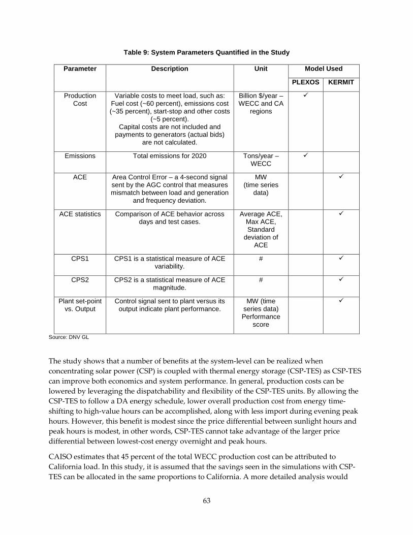
Table 9: System Parameters Quantified in the Study
Parameter Description Unit Model Used
PLEXOS KERMIT
Production Cost
Variable costs to meet load, such as: Fuel cost (~60 percent), emissions cost (~35 percent), start-stop and other costs
(~5 percent). Capital costs are not included and
payments to generators (actual bids) are not calculated.
Billion $/year – WECC and CA
regions
Emissions Total emissions for 2020 Tons/year – WECC
ACE Area Control Error – a 4-second signal sent by the AGC control that measures mismatch between load and generation
and frequency deviation.
MW (time series
data)
ACE statistics Comparison of ACE behavior across days and test cases.
Average ACE, Max ACE, Standard
deviation of ACE
CPS1 CPS1 is a statistical measure of ACE variability.
#
CPS2 CPS2 is a statistical measure of ACE magnitude.
#
Plant set-point vs. Output
Control signal sent to plant versus its output indicate plant performance.
MW (time series data) Performance
score
Source: DNV GL
The study shows that a number of benefits at the system-level can be realized when concentrating solar power (CSP) is coupled with thermal energy storage (CSP-TES) as CSP-TES can improve both economics and system performance. In general, production costs can be lowered by leveraging the dispatchability and flexibility of the CSP-TES units. By allowing the CSP-TES to follow a DA energy schedule, lower overall production cost from energy time-shifting to high-value hours can be accomplished, along with less import during evening peak hours. However, this benefit is modest since the price differential between sunlight hours and peak hours is modest, in other words, CSP-TES cannot take advantage of the larger price differential between lowest-cost energy overnight and peak hours.
CAISO estimates that 45 percent of the total WECC production cost can be attributed to California load. In this study, it is assumed that the savings seen in the simulations with CSP-TES can be allocated in the same proportions to California. A more detailed analysis would
63
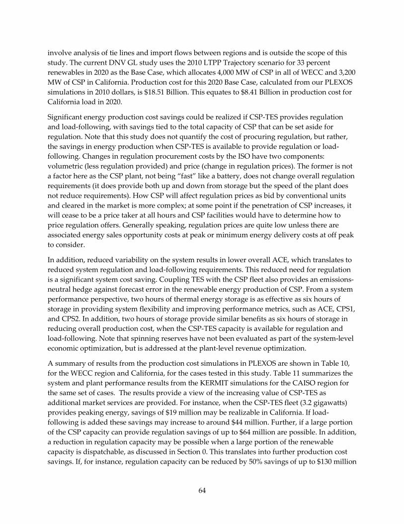
involve analysis of tie lines and import flows between regions and is outside the scope of this study. The current DNV GL study uses the 2010 LTPP Trajectory scenario for 33 percent renewables in 2020 as the Base Case, which allocates 4,000 MW of CSP in all of WECC and 3,200 MW of CSP in California. Production cost for this 2020 Base Case, calculated from our PLEXOS simulations in 2010 dollars, is $18.51 Billion. This equates to $8.41 Billion in production cost for California load in 2020.
Significant energy production cost savings could be realized if CSP-TES provides regulation and load-following, with savings tied to the total capacity of CSP that can be set aside for regulation. Note that this study does not quantify the cost of procuring regulation, but rather, the savings in energy production when CSP-TES is available to provide regulation or load-following. Changes in regulation procurement costs by the ISO have two components: volumetric (less regulation provided) and price (change in regulation prices). The former is not a factor here as the CSP plant, not being “fast” like a battery, does not change overall regulation requirements (it does provide both up and down from storage but the speed of the plant does not reduce requirements). How CSP will affect regulation prices as bid by conventional units and cleared in the market is more complex; at some point if the penetration of CSP increases, it will cease to be a price taker at all hours and CSP facilities would have to determine how to price regulation offers. Generally speaking, regulation prices are quite low unless there are associated energy sales opportunity costs at peak or minimum energy delivery costs at off peak to consider.
In addition, reduced variability on the system results in lower overall ACE, which translates to reduced system regulation and load-following requirements. This reduced need for regulation is a significant system cost saving. Coupling TES with the CSP fleet also provides an emissions-neutral hedge against forecast error in the renewable energy production of CSP. From a system performance perspective, two hours of thermal energy storage is as effective as six hours of storage in providing system flexibility and improving performance metrics, such as ACE, CPS1, and CPS2. In addition, two hours of storage provide similar benefits as six hours of storage in reducing overall production cost, when the CSP-TES capacity is available for regulation and load-following. Note that spinning reserves have not been evaluated as part of the system-level economic optimization, but is addressed at the plant-level revenue optimization.
A summary of results from the production cost simulations in PLEXOS are shown in Table 10, for the WECC region and California, for the cases tested in this study. Table 11 summarizes the system and plant performance results from the KERMIT simulations for the CAISO region for the same set of cases. The results provide a view of the increasing value of CSP-TES as additional market services are provided. For instance, when the CSP-TES fleet (3.2 gigawatts) provides peaking energy, savings of $19 million may be realizable in California. If load-following is added these savings may increase to around $44 million. Further, if a large portion of the CSP capacity can provide regulation savings of up to $64 million are possible. In addition, a reduction in regulation capacity may be possible when a large portion of the renewable capacity is dispatchable, as discussed in Section 0. This translates into further production cost savings. If, for instance, regulation capacity can be reduced by 50% savings of up to $130 million
64
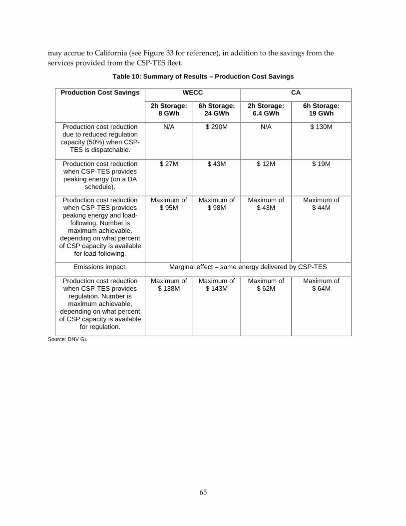
may accrue to California (see Figure 33 for reference), in addition to the savings from the services provided from the CSP-TES fleet.
Table 10: Summary of Results – Production Cost Savings
Production Cost Savings WECC CA
2h Storage: 8 GWh
6h Storage: 24 GWh
2h Storage: 6.4 GWh
6h Storage: 19 GWh
Production cost reduction due to reduced regulation
capacity (50%) when CSP-TES is dispatchable.
N/A $ 290M N/A $ 130M
Production cost reduction when CSP-TES provides peaking energy (on a DA
schedule).
$ 27M $ 43M $ 12M $ 19M
Production cost reduction when CSP-TES provides peaking energy and load-
following. Number is maximum achievable,
depending on what percent of CSP capacity is available
for load-following.
Maximum of $ 95M
Maximum of $ 98M
Maximum of $ 43M
Maximum of $ 44M
Emissions impact. Marginal effect – same energy delivered by CSP-TES
Production cost reduction when CSP-TES provides
regulation. Number is maximum achievable,
depending on what percent of CSP capacity is available
for regulation.
Maximum of $ 138M
Maximum of $ 143M
Maximum of $ 62M
Maximum of $ 64M
Source: DNV GL
65
Table 11: Summary of Results – System and Plant Performance
Plant and System Performance Simulation Results
System performance when adding TES to estimate reduced need for regulation capacity.
Up to 50 percent reduction in regulation results in similar ACE performance as Base Case.
Plant performance when CSP-TES is following a day-ahead schedule.
CSP-TES can follow a day-ahead schedule.
System performance parameters when CSP-TES is following a day-ahead schedule.
15-50 percent reduction in max ACE.
40-90 percent reduction in average ACE.
Reduction of hourly forecast error. TES restores max ACE due to hourly forecast error in 8 out of 10 days.
Ability of CSP-TES to follow a regulation signal. System performance parameters when CSP-TES
provides regulation.
CSP-TES ability to follow regulation signal similar to CC or CT plant.
System performance comparable when regulation is provided by CSP-TES.
CSP-TES plant performance when firming PV plant output.
Transmission capacity firming ability.
CSP-TES capable of reducing PV variability up to 80 percent.
CSP-TES can be dispatched to minimize transmission capacity from a solar resource
area.
Source: DNV GL
66
CHAPTER 5: Thermodynamic Plant Model Simulations This section describes the three CSP technologies and ten TES technologies analyzed in the project and the method used for screening them; a subset of these technologies are then selected for further evaluation and dynamic model development. This subset is intended to encompass technologies that will be economically viable in the near term and that show promise for use in market applications analyzed in subsequent tasks.
Detailed thermodynamic equations and dynamic models are developed for the selected subset of technologies. These models begin with spatially distributed partial differential equations representing the thermodynamics and then are converted to lumped models with sufficient granularity to preserve fidelity. These stand-alone plant models, based on Simulink code, will be used to test the performance of the technologies in response to control signals for various market applications, including regulation and day-ahead energy schedules. These tests are intended to verify whether the technology is suitable for market participation and identify any operational limitations or differences in operational strategy between technologies. By extension, this will also verify whether the system-level results obtained in the system-level (grid) analysis of the project are valid. The plant-level optimization analysis used lower granularity lumped models to represent the thermodynamics and the fidelity of these models for the time ranges of interest was validated by comparison with the more granular models. Data in these models is “generic” and not representative of any manufacturer’s proprietary technology. However, the manufacturers on the advisory committee did agree that the parameters in the generic model were representative and useable for this project.
5.1 CSP and TES Technologies This project analyzes three CSP technologies and ten TES technologies that show promise of success in the near term. Some of the TES technologies are new and there is little understanding of how they perform when coupled with CSP and turbine.
The three CSP technologies refer to the technology used for collecting the solar heat, namely the mirrors and collectors, and the corresponding choice of heat transfer fluid (HTF):
• Central Receiver (Tower): A central tower collects light from the surrounding mirror field. This technology shows promise in that it can deploy high-temperature fluids such as molten salts and has been used in several recent projects globally.
• Linear Receiver (Trough or Fresnel Reflector): Trough reflectors is the most widely used technology today and consists of rows of semi-tubular mirrors (troughs) with HTF pumped along these troughs, typically the HTF used is oil but recently more high-heat HTF have been used.
The thermal storage technologies cover various types of energy storage mediums and tank configurations, namely
67
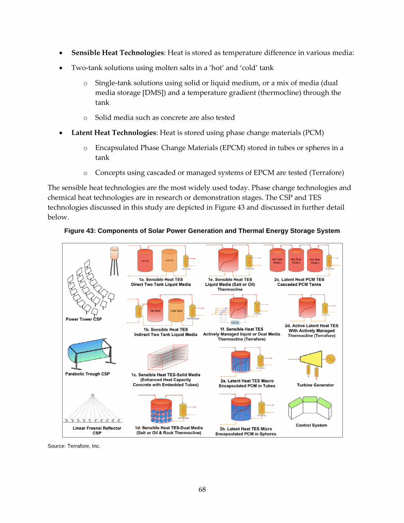
• Sensible Heat Technologies: Heat is stored as temperature difference in various media:
• Two-tank solutions using molten salts in a ‘hot’ and ‘cold’ tank
o Single-tank solutions using solid or liquid medium, or a mix of media (dual media storage [DMS]) and a temperature gradient (thermocline) through the tank
o Solid media such as concrete are also tested
• Latent Heat Technologies: Heat is stored using phase change materials (PCM)
o Encapsulated Phase Change Materials (EPCM) stored in tubes or spheres in a tank
o Concepts using cascaded or managed systems of EPCM are tested (Terrafore)
The sensible heat technologies are the most widely used today. Phase change technologies and chemical heat technologies are in research or demonstration stages. The CSP and TES technologies discussed in this study are depicted in Figure 43 and discussed in further detail below.
Figure 43: Components of Solar Power Generation and Thermal Energy Storage System
Source: Terrafore, Inc.
68
5.1.1 TES technologies The state-of-the-art for TES is a two-tank sensible-heat system, typically with molten salt mixtures as the medium. In this method, the “cold” fluid from a cold tank is pumped through the solar absorber/ receiver and the resulting hot fluid is stored in a hot tank. “Sensible heat” refers to storing thermal energy as a difference in temperature between the two tanks, without any phase change. When heat is required, the hot fluid is pumped from the hot tank to the heat exchanger to produce steam and the colder fluid is then returned to the cold tank. While this TES technology, currently in use at several locations, is easy to operate, it is relatively expensive compared to the SunShot30 cost goal set by US Department of Energy. This is because it requires a large amount of fluid and two large tanks with associated heat tracing and tank maintenance31. The US Department of Energy (DoE) is funding research into thermal storage technologies with the goal to reduce the cost of thermal storage.32
The amount of storage material required and the cost of the TES system can be decreased by increasing the energy density. The energy density can be increased by using “latent heat”, that is, the energy required for phase transition from solid to liquid of inorganic salts in addition to sensible heat. Research funded by the DoE has looked at several approaches to increasing the energy density, either by using phase change materials, by increasing the specific heat of the storage medium (salt mixtures or concrete), or by improving the heat properties of the HTF. Two PCM technologies that showed promise used PCM contained inside small capsules made of shell material, which is compatible with the nitrate molten salt HTF. The encapsulated PCM (EPCM) using small capsules is used in this study.
Yet another approach to reducing the cost is to use a single tank and the principle of thermal stratification to separate the hot and cold layers in the same tank. A major advantage of this thermally stratified sensible heat storage system is that the storage material cost can be significantly reduced by replacing expensive liquid by low cost solid such as rock or granite and by allowing the HTF to flow through the tank. The fluid fills the void between the granite particles. This is called the dual-media thermocline thermal energy storage system. The cost is low because the cost of the storage medium is low and only one tank is required. This technology has been successfully tested in the laboratory but has not been used commercially because of the thermal stratification or thermocline degrades with every charge and discharge cycle requiring a specific operation to restore the thermocline. Therefore, this technology is not modeled in detail in this study.
Another method is to use “thermo-chemical heat”, that is, the enthalpy of reaction of a reversible chemical reaction, which typically is much higher per unit mass converted compared
30 http://www1.eere.energy.gov/solar/pdfs/47927_chapter5.pdf.
31 The following paper proposed a virtual two-tank, eliminating the need for a second physical tank: A.H.Slocum, A.Mitsos et.al, Solar Energy 2011, “Concentrated Solar Power on Demand”, http://www.sciencedirect.com/science/article/pii/S0038092X11001307
32 http://www1.eere.energy.gov/solar/sunshot/csp_storage_awards.html.
69
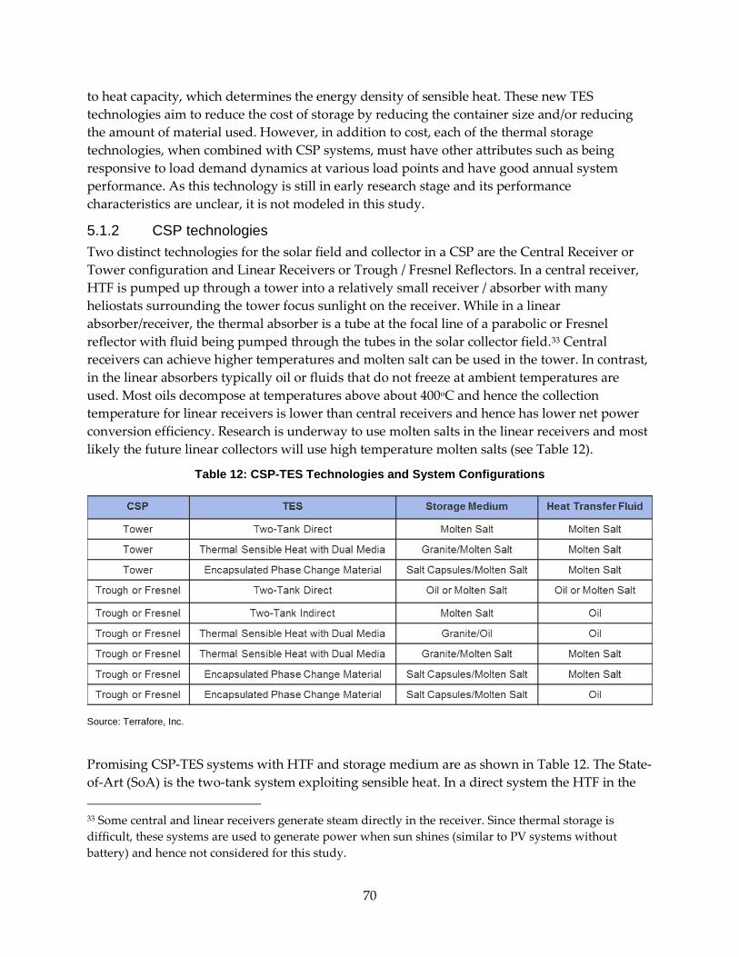
to heat capacity, which determines the energy density of sensible heat. These new TES technologies aim to reduce the cost of storage by reducing the container size and/or reducing the amount of material used. However, in addition to cost, each of the thermal storage technologies, when combined with CSP systems, must have other attributes such as being responsive to load demand dynamics at various load points and have good annual system performance. As this technology is still in early research stage and its performance characteristics are unclear, it is not modeled in this study.
5.1.2 CSP technologies Two distinct technologies for the solar field and collector in a CSP are the Central Receiver or Tower configuration and Linear Receivers or Trough / Fresnel Reflectors. In a central receiver, HTF is pumped up through a tower into a relatively small receiver / absorber with many heliostats surrounding the tower focus sunlight on the receiver. While in a linear absorber/receiver, the thermal absorber is a tube at the focal line of a parabolic or Fresnel reflector with fluid being pumped through the tubes in the solar collector field.33 Central receivers can achieve higher temperatures and molten salt can be used in the tower. In contrast, in the linear absorbers typically oil or fluids that do not freeze at ambient temperatures are used. Most oils decompose at temperatures above about 400oC and hence the collection temperature for linear receivers is lower than central receivers and hence has lower net power conversion efficiency. Research is underway to use molten salts in the linear receivers and most likely the future linear collectors will use high temperature molten salts (see Table 12).
Table 12: CSP-TES Technologies and System Configurations
Source: Terrafore, Inc.
Promising CSP-TES systems with HTF and storage medium are as shown in Table 12. The State-of-Art (SoA) is the two-tank system exploiting sensible heat. In a direct system the HTF in the
33 Some central and linear receivers generate steam directly in the receiver. Since thermal storage is difficult, these systems are used to generate power when sun shines (similar to PV systems without battery) and hence not considered for this study.
70
collectors and the storage system is the same. Most central receiver systems use direct TES with molten salt as HTF and storage medium. As mentioned, currently, linear collector systems (trough and Fresnel CSP) use VP-1 oil as heat transfer medium and store energy in the same fluid as the HTF (direct method) or transfer energy from the oil to molten salt and store energy in a molten salt mixture (indirect method).The conversion efficiency from stored to electrical power is lower (by about 7 percent) due to drop in storage temperature. Both direct and indirect methods are currently used for TES. For the purposes of this analysis, dynamic mathematical models for trough and central receiver technologies are developed. The dynamics of the linear Fresnel collectors is assumed to be similar to the trough technology.
5.1.3 Technological Limits of CSP-TES While the report focuses on technologies that are relatively technologically mature and uses design and operation schemes that are relevant for the next few years in California, this section highlights concepts that have not been proven in practice and challenge limits on operation.
Most CSP-TES technologies have essentially separate solar collector/receiver and storage systems and most commercial systems use surface receivers. Surface receivers are limited in the energy transfer rate per unit area, and consequently in concentration factor. This limitation has led to the development of volumetric receivers, including the DLR concept.34 A concept developed at MIT35 is the CSPonD which is based on direct radiation of the concentrated light into the hot tank, thus also integrating receiver and storage. Moreover, CSPonD uses a single tank with a divider, aiming to incur the capital costs of a single tank but have the thermodynamic advantage of a two-tank system. A proposal from Cyprus Institute36 is the so-called IStore concept which is based on a black-body cavity design.
The report considers the effect of design choices on economic performance. In particular, the relative sizing of power block, solar collector area, and thermal energy storage are considered via two design variables (solar multiple and hours of thermal storage). With conventional operating policies, these two design variables are not entirely independent. For instance, imposing that on design day, the storage must be able to be charged from zero to full charge, implying that the storage hours of the TES cannot be more than the hours of sunshine on the design day. However, in principle, the two design variables are independent of each other and simultaneous techno-economic optimization of design and year-long operation is necessary to determine the optimal technology and configuration for a given market. A technological idea that goes beyond the state of the art is the idea of so-called seasonal thermal energy storage37,38 meaning that multiple days or weeks of storage capacity can be charged in one season and used
34 http://elib.dlr.de/77652/1/Materials.pdf.
35 http://dx.doi.org/10.1016/j.solener.2011.04.010.
36 http://www.cyi.ac.cy/system/files/istore.pdf.
37 https://pangea.stanford.edu/ERE/pdf/IGAstandard/SGW/2012/Forsberg.pdf.
38 http://www.arpa-e.energy.gov/sites/default/files/documents/files/Forsberg.pdf.
71
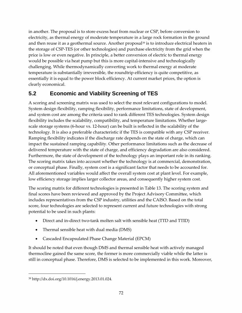
in another. The proposal is to store excess heat from nuclear or CSP, before conversion to electricity, as thermal energy of moderate temperature in a large rock formation in the ground and then reuse it as a geothermal source. Another proposal39 is to introduce electrical heaters in the storage of CSP-TES (or other technologies) and purchase electricity from the grid when the price is low or even negative. In principle, a better conversion of electric to thermal energy would be possible via heat pump but this is more capital-intensive and technologically challenging. While thermodynamically converting work to thermal energy at moderate temperature is substantially irreversible, the roundtrip efficiency is quite competitive, as essentially it is equal to the power block efficiency. At current market prices, the option is clearly economical.
5.2 Economic and Viability Screening of TES A scoring and screening matrix was used to select the most relevant configurations to model. System design flexibility, ramping flexibility, performance limitations, state of development, and system cost are among the criteria used to rank different TES technologies. System design flexibility includes the scalability, compatibility, and temperature limitations. Whether large-scale storage systems (6-hour vs. 12-hour) can be built is reflected in the scalability of the technology. It is also a preferable characteristic if the TES is compatible with any CSP receiver. Ramping flexibility indicates if the discharge rate depends on the state of charge, which can impact the sustained ramping capability. Other performance limitations such as the decrease of delivered temperature with the state of charge, and efficiency degradation are also considered. Furthermore, the state of development of the technology plays an important role in its ranking. The scoring matrix takes into account whether the technology is at commercial, demonstration, or conceptual phase. Finally, system cost is a significant factor that needs to be accounted for. All aforementioned variables would affect the overall system cost at plant level. For example, low efficiency storage implies larger collector areas, and consequently higher system cost.
The scoring matrix for different technologies is presented in Table 13. The scoring system and final scores have been reviewed and approved by the Project Advisory Committee, which includes representatives from the CSP industry, utilities and the CAISO. Based on the total score, four technologies are selected to represent current and future technologies with strong potential to be used in such plants:
• Direct and in-direct two-tank molten salt with sensible heat (TTD and TTID)
• Thermal sensible heat with dual media (DMS)
• Cascaded Encapsulated Phase Change Material (EPCM)
It should be noted that even though DMS and thermal sensible heat with actively managed thermocline gained the same score, the former is more commercially viable while the latter is still in conceptual phase. Therefore, DMS is selected to be implemented in this work. Moreover,
39 http://dx.doi.org/10.1016/j.energy.2013.01.024.
72
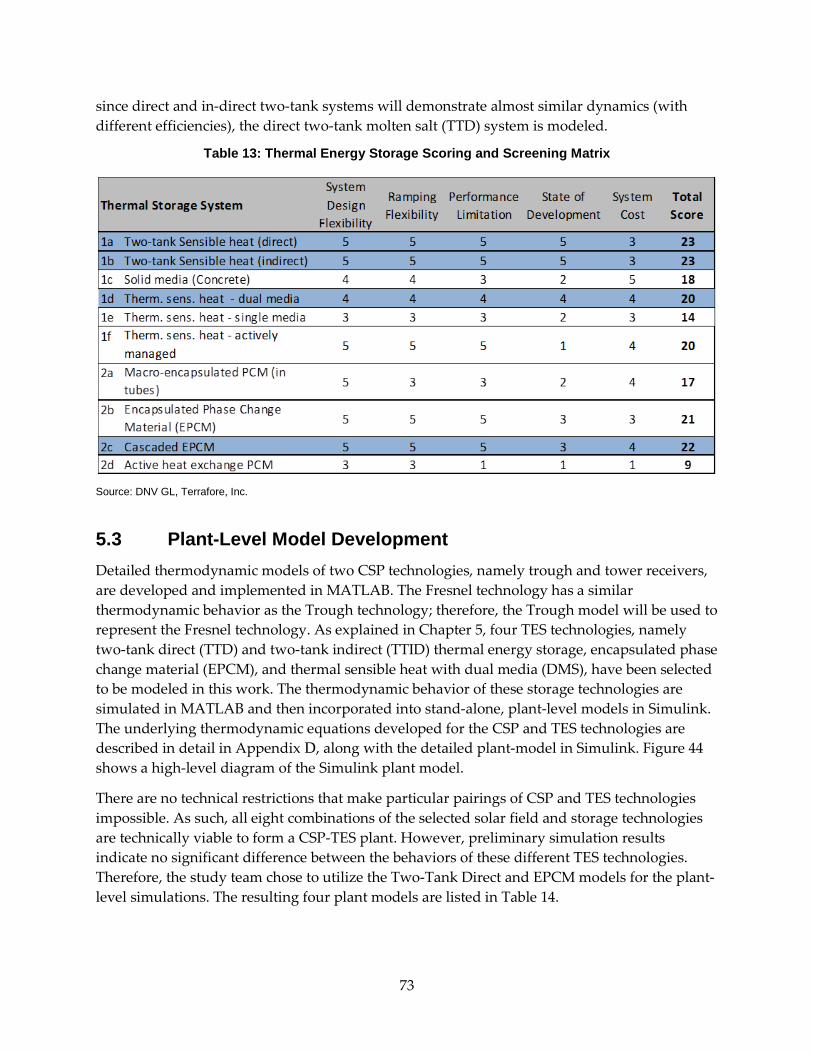
since direct and in-direct two-tank systems will demonstrate almost similar dynamics (with different efficiencies), the direct two-tank molten salt (TTD) system is modeled.
Table 13: Thermal Energy Storage Scoring and Screening Matrix
Source: DNV GL, Terrafore, Inc.
5.3 Plant-Level Model Development Detailed thermodynamic models of two CSP technologies, namely trough and tower receivers, are developed and implemented in MATLAB. The Fresnel technology has a similar thermodynamic behavior as the Trough technology; therefore, the Trough model will be used to represent the Fresnel technology. As explained in Chapter 5, four TES technologies, namely two-tank direct (TTD) and two-tank indirect (TTID) thermal energy storage, encapsulated phase change material (EPCM), and thermal sensible heat with dual media (DMS), have been selected to be modeled in this work. The thermodynamic behavior of these storage technologies are simulated in MATLAB and then incorporated into stand-alone, plant-level models in Simulink. The underlying thermodynamic equations developed for the CSP and TES technologies are described in detail in Appendix D, along with the detailed plant-model in Simulink. Figure 44 shows a high-level diagram of the Simulink plant model.
There are no technical restrictions that make particular pairings of CSP and TES technologies impossible. As such, all eight combinations of the selected solar field and storage technologies are technically viable to form a CSP-TES plant. However, preliminary simulation results indicate no significant difference between the behaviors of these different TES technologies. Therefore, the study team chose to utilize the Two-Tank Direct and EPCM models for the plant-level simulations. The resulting four plant models are listed in Table 14.
73
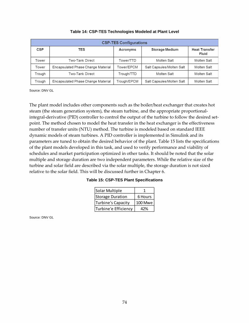
Table 14: CSP-TES Technologies Modeled at Plant Level
Source: DNV GL
The plant model includes other components such as the boiler/heat exchanger that creates hot steam (the steam generation system), the steam turbine, and the appropriate proportional-integral-derivative (PID) controller to control the output of the turbine to follow the desired set-point. The method chosen to model the heat transfer in the heat exchanger is the effectiveness number of transfer units (NTU) method. The turbine is modeled based on standard IEEE dynamic models of steam turbines. A PID controller is implemented in Simulink and its parameters are tuned to obtain the desired behavior of the plant. Table 15 lists the specifications of the plant models developed in this task, and used to verify performance and viability of schedules and market participation optimized in other tasks. It should be noted that the solar multiple and storage duration are two independent parameters. While the relative size of the turbine and solar field are described via the solar multiple, the storage duration is not sized relative to the solar field. This will be discussed further in Chapter 6.
Table 15: CSP-TES Plant Specifications
Source: DNV GL
Solar Multiple 1Storage Duration 6 HoursTurbine's Capacity 100 MweTurbine'e Efficiency 42%
74
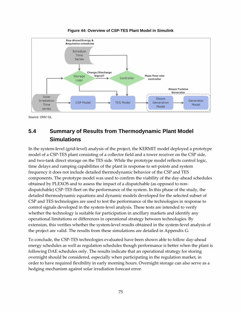
Figure 44: Overview of CSP-TES Plant Model in Simulink
Source: DNV GL
5.4 Summary of Results from Thermodynamic Plant Model Simulations
In the system-level (grid-level) analysis of the project, the KERMIT model deployed a prototype model of a CSP-TES plant consisting of a collector field and a tower receiver on the CSP side, and two-tank direct storage on the TES side. While the prototype model reflects control logic, time delays and ramping capabilities of the plant in response to set-points and system frequency it does not include detailed thermodynamic behavior of the CSP and TES components. The prototype model was used to confirm the viability of the day-ahead schedules obtained by PLEXOS and to assess the impact of a dispatchable (as opposed to non-dispatchable) CSP-TES fleet on the performance of the system. In this phase of the study, the detailed thermodynamic equations and dynamic models developed for the selected subset of CSP and TES technologies are used to test the performance of the technologies in response to control signals developed in the system-level analysis. These tests are intended to verify whether the technology is suitable for participation in ancillary markets and identify any operational limitations or differences in operational strategy between technologies. By extension, this verifies whether the system-level results obtained in the system-level analysis of the project are valid. The results from these simulations are detailed in Appendix G.
To conclude, the CSP-TES technologies evaluated have been shown able to follow day-ahead energy schedules as well as regulation schedules though performance is better when the plant is following DAE schedules only. The results indicate that an operational strategy for storing overnight should be considered, especially when participating in the regulation market, in order to have required flexibility in early morning hours. Overnight storage can also serve as a hedging mechanism against solar irradiation forecast error.
75
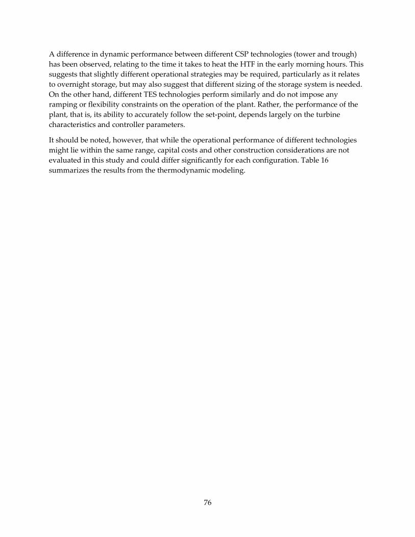
A difference in dynamic performance between different CSP technologies (tower and trough) has been observed, relating to the time it takes to heat the HTF in the early morning hours. This suggests that slightly different operational strategies may be required, particularly as it relates to overnight storage, but may also suggest that different sizing of the storage system is needed. On the other hand, different TES technologies perform similarly and do not impose any ramping or flexibility constraints on the operation of the plant. Rather, the performance of the plant, that is, its ability to accurately follow the set-point, depends largely on the turbine characteristics and controller parameters.
It should be noted, however, that while the operational performance of different technologies might lie within the same range, capital costs and other construction considerations are not evaluated in this study and could differ significantly for each configuration. Table 16 summarizes the results from the thermodynamic modeling.
76
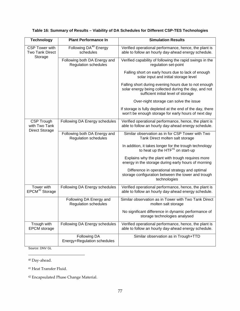
Table 16: Summary of Results – Viability of DA Schedules for Different CSP-TES Technologies
Technology Plant Performance In Simulation Results
CSP Tower with Two Tank Direct
Storage
Following DA40 Energy schedules
Verified operational performance, hence, the plant is able to follow an hourly day-ahead energy schedule.
Following both DA Energy and Regulation schedules
Verified capability of following the rapid swings in the regulation set-point
Falling short on early hours due to lack of enough solar input and initial storage level
Falling short during evening hours due to not enough solar energy being collected during the day, and not
sufficient initial level of storage
Over-night storage can solve the issue
If storage is fully depleted at the end of the day, there won’t be enough storage for early hours of next day
CSP Trough with Two Tank Direct Storage
Following DA Energy schedules Verified operational performance, hence, the plant is able to follow an hourly day-ahead energy schedule.
Following both DA Energy and Regulation schedules
Similar observation as in for CSP Tower with Two Tank Direct molten salt storage
In addition, it takes longer for the trough technology to heat up the HTF41 on start-up
Explains why the plant with trough requires more energy in the storage during early hours of morning
Difference in operational strategy and optimal storage configuration between the tower and trough
technologies
Tower with EPCM42 Storage
Following DA Energy schedules Verified operational performance, hence, the plant is able to follow an hourly day-ahead energy schedule.
Following DA Energy and Regulation schedules
Similar observation as in Tower with Two Tank Direct molten salt storage
No significant difference in dynamic performance of storage technologies analysed
Trough with EPCM storage
Following DA Energy schedules Verified operational performance, hence, the plant is able to follow an hourly day-ahead energy schedule.
Following DA Energy+Regulation schedules
Similar observation as in Trough+TTD
Source: DNV GL
40 Day-ahead.
41 Heat Transfer Fluid.
42 Encapsulated Phase Change Material.
77
CHAPTER 6: Plant Revenue and Configuration Optimization This section discusses the methodology for optimizing participation in Day-Ahead Energy, Regulation, and Spinning Reserve markets for a range of CSP-TES design configurations. Design considerations include the size of the solar field, thermal storage duration and steam power block (steam generator, turbine, and condenser with associated pumps and controls) capacity, along with gas co-firing capabilities. The turbine generator determines the instantaneous capacity of the electrical generation and the steam generator and condensers are sized as dictated by the turbine generator set. We use the term “turbine” in this report to denote the capacity of the steam power block. Dispatch is optimized to maximize plant revenue across markets for a given CSP-TES design. The results are presented in Chapter 7. Further, a cost-benefit analysis highlights the trade-offs between revenue and capital cost in sizing components and choosing the optimal design for CSP-TES in the California market.
6.1 CSP-TES Components and Relative Sizing The overall design of the CSP-TES plant will affect its ability to participate in various markets and maximize its revenue. At a high level, the primary components of a CSP-TES plant are the solar field (collector and receiver), the thermal energy storage system, and the steam turbine, as shown in Figure 45. In addition, a gas boiler may be present to supplement the solar energy when solar output is insufficient to operate the turbine generator. This section identifies the optimal, relative sizing of these components in order to maximize revenue for the plant when participating in energy and ancillary services markets in California. We are making the assumption that CSP-TES plants will be designed and built such that economies/diseconomies of scale have been considered, and have performed the optimization of configurations without regard to scale limitations. The results obtained do not lead to huge variations in configuration size (as in hypothetical five days of TES capacity or 20 minutes, which would create scale issues).
Figure 45: CSP Configuration Schematic Showing Permissible Energy Flows
G
+Solar field
Thermal storage
Gas burner
Turbine generator
Energy output to grid
Source: DNV GL
78
The relative sizing of these basic components - solar field, thermal storage, turbine, and gas co-firing capability - is captured via a few simple metrics, described in detail in the next section.
6.1.1 Solar Multiple, Storage Duration, and Turbine Capacity The solar multiple (SM) is a measure of the size of the solar field relative to the turbine-generator capacity. A value of one for SM suggests that the solar field is sized to nominally match the turbine. Consider the case when the solar output is directly converted to steam and is passed to the turbine generator for electric energy production. An SM of one implies that on the design day, the steam production is just sufficient to operate the turbine generator at rated electric capacity. Consequently, SM > 1 implies that in some hours, energy is collected by the solar field at a higher rate than can be output by the steam generator, hence a thermal energy storage system is needed or else energy is wasted. By contrast, for SM < 1 the solar field cannot produce enough energy even at peak production to supply the full turbine capacity. In this case, the turbine would have spare capacity unless thermal storage is used to collect energy during a longer time period for dispatch in a shorter time interval.
For this analysis, the size of the solar field is assumed constant and, hence, the collected solar energy is the same for all configurations. This will allow an easy comparison between CSP-TES configurations, as annual revenue is tied to a fixed solar energy input. In addition, the solar field is the largest capital expenditure of the plant. Chapter 6 will provide an analysis of the trade-off between capital cost for these components, and revenue accrued by various configurations. For our analysis, therefore, variation in solar multiple implies changing the size of the turbine generator, relative to the solar field. In other words, SM > 1 implies that the turbine generator is nominally undersized for the solar field, and that some energy output of the solar field will need to be stored and output shifted to times when the turbine has available capacity. Without thermal storage in this case, for some times in the year, solar energy is wasted. Conversely, SM < 1 implies that the turbine generator is nominally oversized relative to the solar field, and there will be spare turbine capacity even at hours of peak solar production. For example, if SM = 2, the turbine is sized such that half the solar energy output on the peak solar production hour of the year can be used directly to produce electric energy. If SM= 0.5, the turbine is sized such that twice the solar energy output on the peak solar production hour of the year can be used directly to produce electric energy.
The thermal power capacity (that is, maximum heat transfer rate) of the TES system is assumed to match the capacity of the turbine generator. In other words, the TES system can produce enough steam to operate the turbine generator at rated maximum capacity, even in hours when there is no solar field output. This parameter can be translated into the thermal power capacity of the TES. This assumption implies that the steam generation from the TES is sized to the full power rating of the steam power block; and that the power block could operate without parallel energy supplied directly from the solar field that did not first go into storage. The energy capacity of the TES system is described by the duration (hours) it can supply the turbine at maximum rated capacity. For example, if the combined efficiency of the thermal storage to electric energy system is 40 percent, and the turbine generator capacity is 100 MWe, the power capacity of the TES system is 100/0.4 = 250 MWt. With a two-hour duration, the TES system will
79
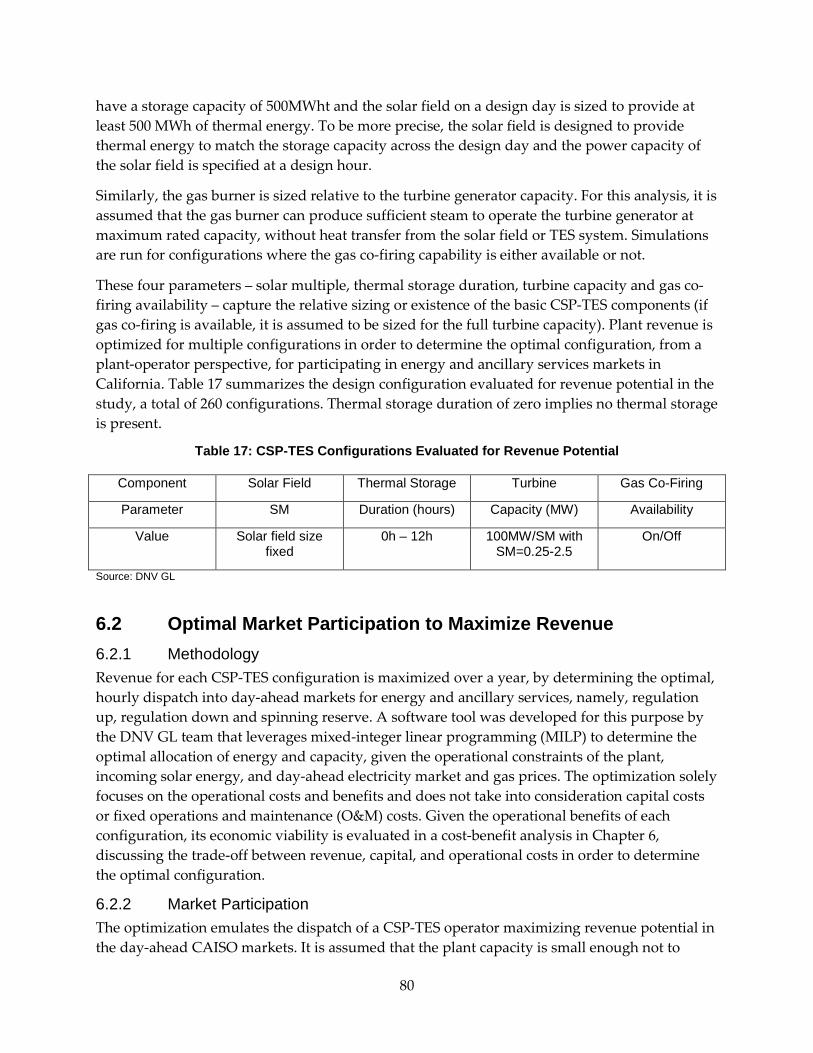
have a storage capacity of 500MWht and the solar field on a design day is sized to provide at least 500 MWh of thermal energy. To be more precise, the solar field is designed to provide thermal energy to match the storage capacity across the design day and the power capacity of the solar field is specified at a design hour.
Similarly, the gas burner is sized relative to the turbine generator capacity. For this analysis, it is assumed that the gas burner can produce sufficient steam to operate the turbine generator at maximum rated capacity, without heat transfer from the solar field or TES system. Simulations are run for configurations where the gas co-firing capability is either available or not.
These four parameters – solar multiple, thermal storage duration, turbine capacity and gas co-firing availability – capture the relative sizing or existence of the basic CSP-TES components (if gas co-firing is available, it is assumed to be sized for the full turbine capacity). Plant revenue is optimized for multiple configurations in order to determine the optimal configuration, from a plant-operator perspective, for participating in energy and ancillary services markets in California. Table 17 summarizes the design configuration evaluated for revenue potential in the study, a total of 260 configurations. Thermal storage duration of zero implies no thermal storage is present.
Table 17: CSP-TES Configurations Evaluated for Revenue Potential
Component Solar Field Thermal Storage Turbine Gas Co-Firing
Parameter SM Duration (hours) Capacity (MW) Availability
Value Solar field size fixed
0h – 12h 100MW/SM with SM=0.25-2.5
On/Off
Source: DNV GL
6.2 Optimal Market Participation to Maximize Revenue 6.2.1 Methodology Revenue for each CSP-TES configuration is maximized over a year, by determining the optimal, hourly dispatch into day-ahead markets for energy and ancillary services, namely, regulation up, regulation down and spinning reserve. A software tool was developed for this purpose by the DNV GL team that leverages mixed-integer linear programming (MILP) to determine the optimal allocation of energy and capacity, given the operational constraints of the plant, incoming solar energy, and day-ahead electricity market and gas prices. The optimization solely focuses on the operational costs and benefits and does not take into consideration capital costs or fixed operations and maintenance (O&M) costs. Given the operational benefits of each configuration, its economic viability is evaluated in a cost-benefit analysis in Chapter 6, discussing the trade-off between revenue, capital, and operational costs in order to determine the optimal configuration.
6.2.2 Market Participation The optimization emulates the dispatch of a CSP-TES operator maximizing revenue potential in the day-ahead CAISO markets. It is assumed that the plant capacity is small enough not to
80
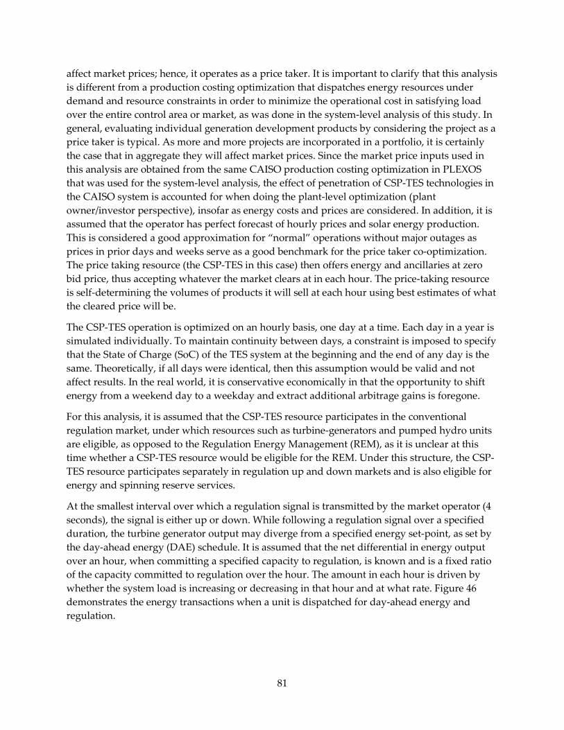
affect market prices; hence, it operates as a price taker. It is important to clarify that this analysis is different from a production costing optimization that dispatches energy resources under demand and resource constraints in order to minimize the operational cost in satisfying load over the entire control area or market, as was done in the system-level analysis of this study. In general, evaluating individual generation development products by considering the project as a price taker is typical. As more and more projects are incorporated in a portfolio, it is certainly the case that in aggregate they will affect market prices. Since the market price inputs used in this analysis are obtained from the same CAISO production costing optimization in PLEXOS that was used for the system-level analysis, the effect of penetration of CSP-TES technologies in the CAISO system is accounted for when doing the plant-level optimization (plant owner/investor perspective), insofar as energy costs and prices are considered. In addition, it is assumed that the operator has perfect forecast of hourly prices and solar energy production. This is considered a good approximation for “normal” operations without major outages as prices in prior days and weeks serve as a good benchmark for the price taker co-optimization. The price taking resource (the CSP-TES in this case) then offers energy and ancillaries at zero bid price, thus accepting whatever the market clears at in each hour. The price-taking resource is self-determining the volumes of products it will sell at each hour using best estimates of what the cleared price will be.
The CSP-TES operation is optimized on an hourly basis, one day at a time. Each day in a year is simulated individually. To maintain continuity between days, a constraint is imposed to specify that the State of Charge (SoC) of the TES system at the beginning and the end of any day is the same. Theoretically, if all days were identical, then this assumption would be valid and not affect results. In the real world, it is conservative economically in that the opportunity to shift energy from a weekend day to a weekday and extract additional arbitrage gains is foregone.
For this analysis, it is assumed that the CSP-TES resource participates in the conventional regulation market, under which resources such as turbine-generators and pumped hydro units are eligible, as opposed to the Regulation Energy Management (REM), as it is unclear at this time whether a CSP-TES resource would be eligible for the REM. Under this structure, the CSP-TES resource participates separately in regulation up and down markets and is also eligible for energy and spinning reserve services.
At the smallest interval over which a regulation signal is transmitted by the market operator (4 seconds), the signal is either up or down. While following a regulation signal over a specified duration, the turbine generator output may diverge from a specified energy set-point, as set by the day-ahead energy (DAE) schedule. It is assumed that the net differential in energy output over an hour, when committing a specified capacity to regulation, is known and is a fixed ratio of the capacity committed to regulation over the hour. The amount in each hour is driven by whether the system load is increasing or decreasing in that hour and at what rate. Figure 46 demonstrates the energy transactions when a unit is dispatched for day-ahead energy and regulation.
81
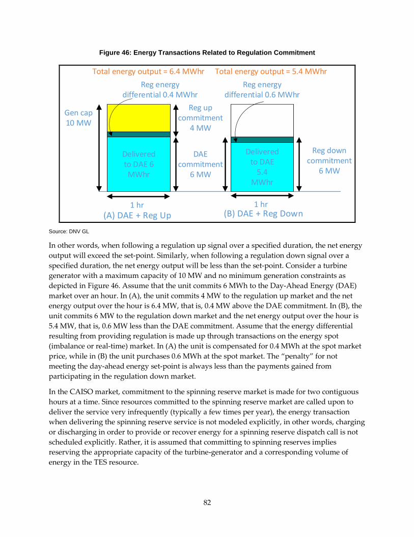
Figure 46: Energy Transactions Related to Regulation Commitment
Gen cap 10 MW
DAE commitment
6 MW
Reg up commitment
4 MW
Delivered to DAE 6 MWhr
Reg energy differential 0.4 MWhr
1 hr
Reg down commitment
6 MW
Delivered to DAE
5.4 MWhr
Reg energy differential 0.6 MWhr
Total energy output = 5.4 MWhrTotal energy output = 6.4 MWhr
1 hr(A) DAE + Reg Up (B) DAE + Reg Down
Source: DNV GL
In other words, when following a regulation up signal over a specified duration, the net energy output will exceed the set-point. Similarly, when following a regulation down signal over a specified duration, the net energy output will be less than the set-point. Consider a turbine generator with a maximum capacity of 10 MW and no minimum generation constraints as depicted in Figure 46. Assume that the unit commits 6 MWh to the Day-Ahead Energy (DAE) market over an hour. In (A), the unit commits 4 MW to the regulation up market and the net energy output over the hour is 6.4 MW, that is, 0.4 MW above the DAE commitment. In (B), the unit commits 6 MW to the regulation down market and the net energy output over the hour is 5.4 MW, that is, 0.6 MW less than the DAE commitment. Assume that the energy differential resulting from providing regulation is made up through transactions on the energy spot (imbalance or real-time) market. In (A) the unit is compensated for 0.4 MWh at the spot market price, while in (B) the unit purchases 0.6 MWh at the spot market. The “penalty” for not meeting the day-ahead energy set-point is always less than the payments gained from participating in the regulation down market.
In the CAISO market, commitment to the spinning reserve market is made for two contiguous hours at a time. Since resources committed to the spinning reserve market are called upon to deliver the service very infrequently (typically a few times per year), the energy transaction when delivering the spinning reserve service is not modeled explicitly, in other words, charging or discharging in order to provide or recover energy for a spinning reserve dispatch call is not scheduled explicitly. Rather, it is assumed that committing to spinning reserves implies reserving the appropriate capacity of the turbine-generator and a corresponding volume of energy in the TES resource.
82
The operational constraints of the optimization problem are set up according to the operational characteristics of the various components, including the following:
• Energy flows are formulated according to Figure 45.
• The TES unit can charge and discharge over the same time interval.
• The state of charge of the TES unit at the beginning of a day is specified to half of rated capacity. At the end of the day, the state of charge is at half or higher.
• The turbine has a minimum output level of 10 percent of rated capacity
• It is assumed that there is capacity for steam storage that permits the generator to ramp faster than conventional units without steam storage.
• The start-up energy costs and shut-down energy losses associated with the on-off transitions of the turbine generator and gas co-firing unit are assumed to be zero.
• The efficiencies of the turbine generator and gas co-firing unit are assumed to be constant with respect to loading level.
The exact mathematical formulation of the optimization problem is presented in Appendix F. Generator capacity constraints for commitment to day-ahead energy and regulation are shown in Figure 47. The capacity of the generator in excess of its day-ahead energy commitment is available for regulation up. The capacity of the generator in between the minimum capacity and the day-ahead energy commitment is available for regulation down. The generator has to be ‘ON’ meaning that it is operating at at-least the minimum level to commit to any market – DAE, regulation or spinning reserve.
The results of the optimization are presented in Chapter 7.
Figure 47: Generator Capacity Constraints for DAE and Regulation Commitment
(A) DAE commitment > Min generation level
DAE commit
ment
Gen min level
Reg up
Reg down
(B) DAE commitment = Min generation level
Gen min level =
DAE commit
ment
Reg up
Available generator capacities for reg up and reg down
Source: DNV GL
83
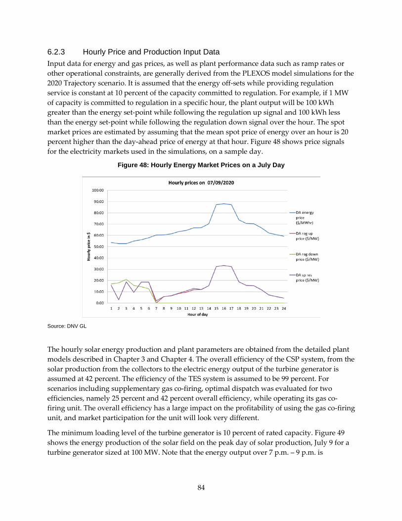
6.2.3 Hourly Price and Production Input Data Input data for energy and gas prices, as well as plant performance data such as ramp rates or other operational constraints, are generally derived from the PLEXOS model simulations for the 2020 Trajectory scenario. It is assumed that the energy off-sets while providing regulation service is constant at 10 percent of the capacity committed to regulation. For example, if 1 MW of capacity is committed to regulation in a specific hour, the plant output will be 100 kWh greater than the energy set-point while following the regulation up signal and 100 kWh less than the energy set-point while following the regulation down signal over the hour. The spot market prices are estimated by assuming that the mean spot price of energy over an hour is 20 percent higher than the day-ahead price of energy at that hour. Figure 48 shows price signals for the electricity markets used in the simulations, on a sample day.
Figure 48: Hourly Energy Market Prices on a July Day
Source: DNV GL
The hourly solar energy production and plant parameters are obtained from the detailed plant models described in Chapter 3 and Chapter 4. The overall efficiency of the CSP system, from the solar production from the collectors to the electric energy output of the turbine generator is assumed at 42 percent. The efficiency of the TES system is assumed to be 99 percent. For scenarios including supplementary gas co-firing, optimal dispatch was evaluated for two efficiencies, namely 25 percent and 42 percent overall efficiency, while operating its gas co-firing unit. The overall efficiency has a large impact on the profitability of using the gas co-firing unit, and market participation for the unit will look very different.
The minimum loading level of the turbine generator is 10 percent of rated capacity. Figure 49 shows the energy production of the solar field on the peak day of solar production, July 9 for a turbine generator sized at 100 MW. Note that the energy output over 7 p.m. – 9 p.m. is
84
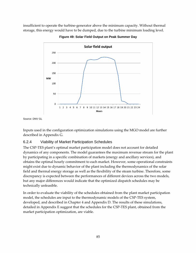
insufficient to operate the turbine-generator above the minimum capacity. Without thermal storage, this energy would have to be dumped, due to the turbine minimum loading level.
Figure 49: Solar Field Output on Peak Summer Day
Source: DNV GL
Inputs used in the configuration optimization simulations using the MGO model are further described in Appendix G.
6.2.4 Viability of Market Participation Schedules The CSP-TES plant’s optimal market participation model does not account for detailed dynamics of any components. The model guarantees the maximum revenue stream for the plant by participating in a specific combination of markets (energy and ancillary services), and obtains the optimal hourly commitment to each market. However, some operational constraints might exist due to dynamic behavior of the plant including the thermodynamics of the solar field and thermal energy storage as well as the flexibility of the steam turbine. Therefore, some discrepancy is expected between the performances of different devices across the two models, but any major differences would indicate that the optimized dispatch schedules may be technically unfeasible.
In order to evaluate the viability of the schedules obtained from the plant market participation model, the schedules are input to the thermodynamic models of the CSP-TES system, developed, and described in Chapter 4 and Appendix D. The results of these simulations, detailed in Appendix E suggest that the schedules for the CSP-TES plant, obtained from the market participation optimization, are viable.
85
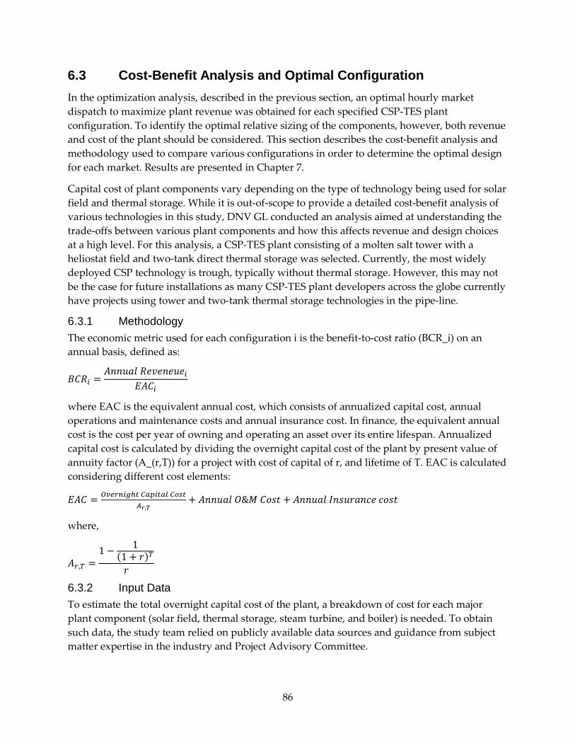
6.3 Cost-Benefit Analysis and Optimal Configuration In the optimization analysis, described in the previous section, an optimal hourly market dispatch to maximize plant revenue was obtained for each specified CSP-TES plant configuration. To identify the optimal relative sizing of the components, however, both revenue and cost of the plant should be considered. This section describes the cost-benefit analysis and methodology used to compare various configurations in order to determine the optimal design for each market. Results are presented in Chapter 7.
Capital cost of plant components vary depending on the type of technology being used for solar field and thermal storage. While it is out-of-scope to provide a detailed cost-benefit analysis of various technologies in this study, DNV GL conducted an analysis aimed at understanding the trade-offs between various plant components and how this affects revenue and design choices at a high level. For this analysis, a CSP-TES plant consisting of a molten salt tower with a heliostat field and two-tank direct thermal storage was selected. Currently, the most widely deployed CSP technology is trough, typically without thermal storage. However, this may not be the case for future installations as many CSP-TES plant developers across the globe currently have projects using tower and two-tank thermal storage technologies in the pipe-line.
6.3.1 Methodology The economic metric used for each configuration i is the benefit-to-cost ratio (BCR_i) on an annual basis, defined as:
𝐵𝐶𝑅𝑖 =𝐴𝑛𝑛𝑢𝑎𝑙 𝑅𝑒𝑣𝑒𝑛𝑒𝑢𝑒𝑖
𝐸𝐴𝐶𝑖
where EAC is the equivalent annual cost, which consists of annualized capital cost, annual operations and maintenance costs and annual insurance cost. In finance, the equivalent annual cost is the cost per year of owning and operating an asset over its entire lifespan. Annualized capital cost is calculated by dividing the overnight capital cost of the plant by present value of annuity factor (A_(r,T)) for a project with cost of capital of r, and lifetime of T. EAC is calculated considering different cost elements:
𝐸𝐴𝐶 = 𝑂𝑣𝑒𝑟𝑛𝑖𝑔ℎ𝑡 𝐶𝑎𝑝𝑖𝑡𝑎𝑙 𝐶𝑜𝑠𝑡𝐴𝑟,𝑇
+ 𝐴𝑛𝑛𝑢𝑎𝑙 𝑂&𝑀 𝐶𝑜𝑠𝑡 + 𝐴𝑛𝑛𝑢𝑎𝑙 𝐼𝑛𝑠𝑢𝑟𝑎𝑛𝑐𝑒 𝑐𝑜𝑠𝑡
where,
𝐴𝑟,𝑇 =1 − 1
(1 + 𝑟)𝑇𝑟
6.3.2 Input Data To estimate the total overnight capital cost of the plant, a breakdown of cost for each major plant component (solar field, thermal storage, steam turbine, and boiler) is needed. To obtain such data, the study team relied on publicly available data sources and guidance from subject matter expertise in the industry and Project Advisory Committee.
86
The current CSP market is dominated by parabolic trough technologies, which are used in more than 80 percent of CSP power plants in operation or under construction. As a consequence, most of the available cost information refers to parabolic trough systems. The cost data for parabolic trough systems are also the most reliable, albeit still uncertain, because it is the most mature CSP technology. However, the project costs available from recently completed projects or projects under construction span a wide range as several factors, such as contractual and financing conditions, impact the overall cost significantly. Table 18 lists the cost of several parabolic trough systems available in literature.43
Table 18: Capital Costs and Key Characteristics of Parabolic Trough Solar – Plant
Source: DNV GL
The total cost of the heliostat solar field and tower technology was estimated at $174M, with a 20 percent cost reduction by 2020 assumed. This value is taken from the SAM model44 for a plant installed in southern California. Since the solar field is kept constant across all configurations and all possible market participations, this cost element is common among all cases.45
Cost estimates of TES systems include storage materials and ancillary equipment for charging and discharging. Sensible heat storage, including a tank for the storage medium and the equipment for charge/discharge, is less expensive than other technologies. Storage media (e.g., water, soil, rocks, concrete or molten salts) are usually inexpensive materials relative to other components of the TES system. However, sensible heat storage requires large volume due to their low energy density. Moreover, they need a proper design to maintain a constant temperature for energy discharge. Finally, the container needs to have an effective thermal
43 Renewable Power Generation Cost in 2012: An Overview, IRENA Report, 2013.
44 https://sam.nrel.gov/
45 It should be noted that Department of Energy’s (DOE) SunShot Initiative goal is to have installed solar field costs of $75 per square meter by 2020.
87
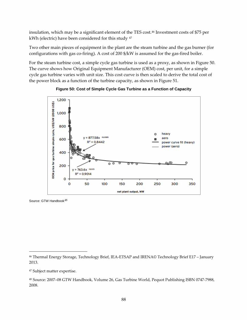
insulation, which may be a significant element of the TES cost.46 Investment costs of $75 per kWh (electric) have been considered for this study 47
Two other main pieces of equipment in the plant are the steam turbine and the gas burner (for configurations with gas co-firing). A cost of 200 $/kW is assumed for the gas-fired boiler.
For the steam turbine cost, a simple cycle gas turbine is used as a proxy, as shown in Figure 50. The curve shows how Original Equipment Manufacturer (OEM) cost, per unit, for a simple cycle gas turbine varies with unit size. This cost curve is then scaled to derive the total cost of the power block as a function of the turbine capacity, as shown in Figure 51.
Figure 50: Cost of Simple Cycle Gas Turbine as a Function of Capacity
Source: GTW Handbook48
46 Thermal Energy Storage, Technology Brief, IEA-ETSAP and IRENA© Technology Brief E17 – January 2013.
47 Subject matter expertise.
48 Source: 2007–08 GTW Handbook, Volume 26, Gas Turbine World, Pequot Publishing ISBN 0747-7988, 2008.
88
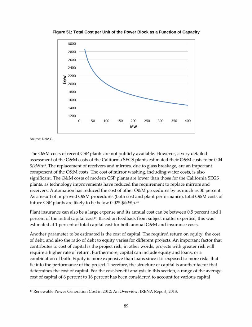
Figure 51: Total Cost per Unit of the Power Block as a Function of Capacity
Source: DNV GL
The O&M costs of recent CSP plants are not publicly available. However, a very detailed assessment of the O&M costs of the California SEGS plants estimated their O&M costs to be 0.04 $/kWh49. The replacement of receivers and mirrors, due to glass breakage, are an important component of the O&M costs. The cost of mirror washing, including water costs, is also significant. The O&M costs of modern CSP plants are lower than those for the California SEGS plants, as technology improvements have reduced the requirement to replace mirrors and receivers. Automation has reduced the cost of other O&M procedures by as much as 30 percent. As a result of improved O&M procedures (both cost and plant performance), total O&M costs of future CSP plants are likely to be below 0.025 $/kWh.49
Plant insurance can also be a large expense and its annual cost can be between 0.5 percent and 1 percent of the initial capital cost49. Based on feedback from subject matter expertise, this was estimated at 1 percent of total capital cost for both annual O&M and insurance costs.
Another parameter to be estimated is the cost of capital. The required return on equity, the cost of debt, and also the ratio of debt to equity varies for different projects. An important factor that contributes to cost of capital is the project risk, in other words, projects with greater risk will require a higher rate of return. Furthermore, capital can include equity and loans, or a combination of both. Equity is more expensive than loans since it is exposed to more risks that tie into the performance of the project. Therefore, the structure of capital is another factor that determines the cost of capital. For the cost-benefit analysis in this section, a range of the average cost of capital of 6 percent to 16 percent has been considered to account for various capital
49 Renewable Power Generation Cost in 2012: An Overview, IRENA Report, 2013.
89
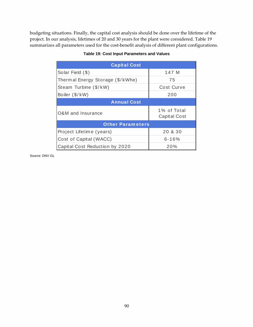
budgeting situations. Finally, the capital cost analysis should be done over the lifetime of the project. In our analysis, lifetimes of 20 and 30 years for the plant were considered. Table 19 summarizes all parameters used for the cost-benefit analysis of different plant configurations.
Table 19: Cost Input Parameters and Values
Source: DNV GL
Solar Field ($) 147 MThermal Energy Storage ($/kWhe) 75Steam Turbine ($/kW) Cost CurveBoiler ($/kW) 200
O&M and Insurance 1% of Total Capital Cost
Project Lifetime (years) 20 & 30Cost of Capital (WACC) 6-16%Capital Cost Reduction by 2020 20%
Capital Cost
Annual Cost
Other Parameters
90
CHAPTER 7: Results: Plant Revenue and Configuration Optimization This section presents the modeling results from the optimization analysis, where CSP-TES participation across markets is optimized to maximize revenue, and the cost-benefit analysis, which will guide the selection of the optimal design for each market. The optimization and cost-benefit analysis are performed across a range of plant configurations, as outlined in Table 17, and according to the methodology described in Chapter 6, in order to assess the impact of the relative sizing of the major design components: Solar field, thermal storage, turbine, and gas co-firing capability.
7.1 CSP-TES Systems with No Gas Co-Firing Capability The following sub-sections present the results from the market optimization for CSP-TES plants without gas co-firing capability, for three market participation schemes: 1) Day-Ahead Energy (DAE) only, 2) DAE and Regulation markets, and 3) DAE, Regulation and Spinning Reserves markets. The CSP-TES configurations with the highest revenue potential and the highest benefit-to-cost ratio in each market scheme are identified
7.1.1 Day-Ahead Energy Market Only In a first step, participation in the day-ahead market is evaluated, and revenue is optimized for various configurations over the course of a year. Figure 52 shows the resulting hourly dispatch for a set of configurations for a sample day. Multiple values for solar multiple (SM) and storage duration are shown in the plot, representing four different CSP-TES plant designs. For all configurations, the solar field is sized for a 100 MW turbine and since the only energy input to the plant is from the sun all plants receive the same energy input. This allows for an apples-to-apples comparison of the revenue captured between the different plants. The solar energy input to the plant is shown in the chart, along with day-ahead energy price modelled for the sample day. The figure highlights how different plant designs will result in highly different market behavior when the goal is to capture the highest possible revenue, driven in part by energy and capacity constraints as implied by design and in part by market prices.
91
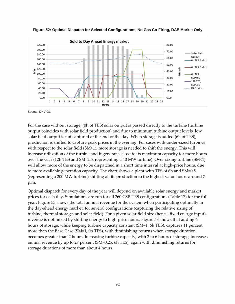
Figure 52: Optimal Dispatch for Selected Configurations, No Gas Co-Firing, DAE Market Only
Source: DNV GL
For the case without storage, (0h of TES) solar output is passed directly to the turbine (turbine output coincides with solar field production) and due to minimum turbine output levels, low solar field output is not captured at the end of the day. When storage is added (6h of TES), production is shifted to capture peak prices in the evening. For cases with under-sized turbines with respect to the solar field (SM>1), more storage is needed to shift the energy. This will increase utilization of the turbine and it generates close to its maximum capacity for more hours over the year (12h TES and SM=2.5, representing a 40 MW turbine). Over-sizing turbine (SM<1) will allow more of the energy to be dispatched in a short time interval at high-price hours, due to more available generation capacity. The chart shows a plant with TES of 6h and SM=0.5 (representing a 200 MW turbine) shifting all its production to the highest-value hours around 7 p.m.
Optimal dispatch for every day of the year will depend on available solar energy and market prices for each day. Simulations are run for all 260 CSP-TES configurations (Table 17) for the full year. Figure 53 shows the total annual revenue for the system when participating optimally in the day-ahead energy market, for several configurations (capturing the relative sizing of turbine, thermal storage, and solar field). For a given solar field size (hence, fixed energy input), revenue is optimized by shifting energy to high-price hours. Figure 53 shows that adding 6 hours of storage, while keeping turbine capacity constant (SM=1, 6h TES), captures 11 percent more than the Base Case (SM=1, 0h TES), with diminishing returns when storage duration becomes greater than 2 hours. Increasing turbine capacity, with 2 to 6 hours of storage, increases annual revenue by up to 27 percent (SM=0.25, 6h TES), again with diminishing returns for storage durations of more than about 4 hours.
92
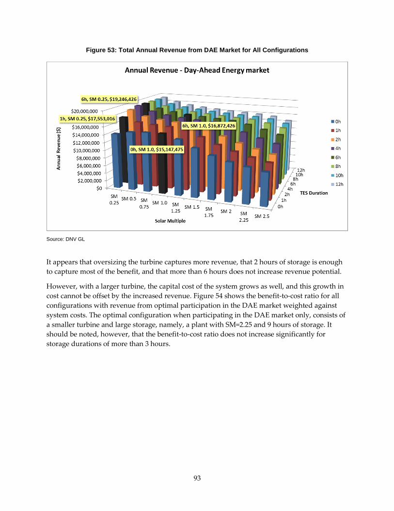
Figure 53: Total Annual Revenue from DAE Market for All Configurations
Source: DNV GL
It appears that oversizing the turbine captures more revenue, that 2 hours of storage is enough to capture most of the benefit, and that more than 6 hours does not increase revenue potential.
However, with a larger turbine, the capital cost of the system grows as well, and this growth in cost cannot be offset by the increased revenue. Figure 54 shows the benefit-to-cost ratio for all configurations with revenue from optimal participation in the DAE market weighted against system costs. The optimal configuration when participating in the DAE market only, consists of a smaller turbine and large storage, namely, a plant with SM=2.25 and 9 hours of storage. It should be noted, however, that the benefit-to-cost ratio does not increase significantly for storage durations of more than 3 hours.
93
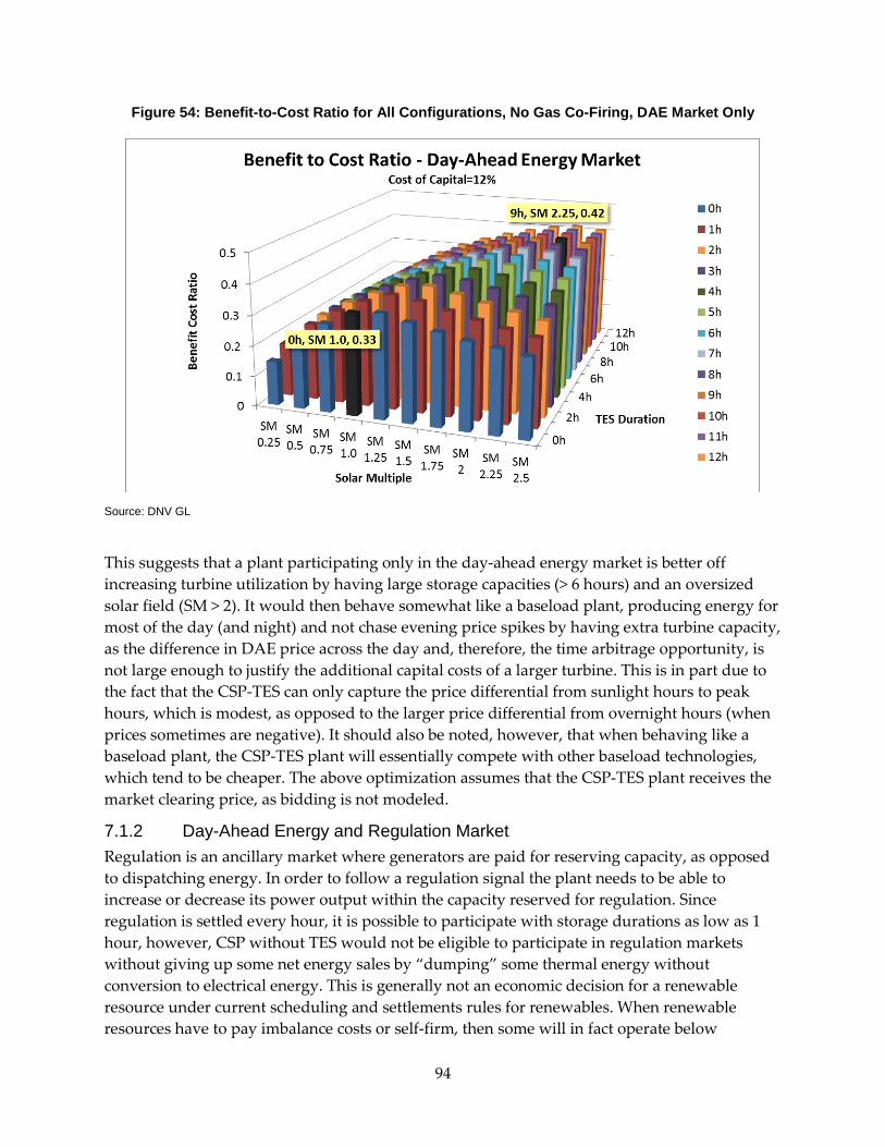
Figure 54: Benefit-to-Cost Ratio for All Configurations, No Gas Co-Firing, DAE Market Only
Source: DNV GL
This suggests that a plant participating only in the day-ahead energy market is better off increasing turbine utilization by having large storage capacities (> 6 hours) and an oversized solar field (SM > 2). It would then behave somewhat like a baseload plant, producing energy for most of the day (and night) and not chase evening price spikes by having extra turbine capacity, as the difference in DAE price across the day and, therefore, the time arbitrage opportunity, is not large enough to justify the additional capital costs of a larger turbine. This is in part due to the fact that the CSP-TES can only capture the price differential from sunlight hours to peak hours, which is modest, as opposed to the larger price differential from overnight hours (when prices sometimes are negative). It should also be noted, however, that when behaving like a baseload plant, the CSP-TES plant will essentially compete with other baseload technologies, which tend to be cheaper. The above optimization assumes that the CSP-TES plant receives the market clearing price, as bidding is not modeled.
7.1.2 Day-Ahead Energy and Regulation Market Regulation is an ancillary market where generators are paid for reserving capacity, as opposed to dispatching energy. In order to follow a regulation signal the plant needs to be able to increase or decrease its power output within the capacity reserved for regulation. Since regulation is settled every hour, it is possible to participate with storage durations as low as 1 hour, however, CSP without TES would not be eligible to participate in regulation markets without giving up some net energy sales by “dumping” some thermal energy without conversion to electrical energy. This is generally not an economic decision for a renewable resource under current scheduling and settlements rules for renewables. When renewable resources have to pay imbalance costs or self-firm, then some will in fact operate below
94
instantaneous capacity so as to minimize imbalance charges. Due to the high value of regulation during certain hours (peak and morning ramp for instance), and the way in which it is paid, the optimal dispatch for a CSP-TES plant, and by extension the optimal design, will look very different from the case where only the DAE market is considered. For instance, increasing turbine capacity relative to the solar field, with small amounts of storage, will maximize participation in regulation markets as opposed to energy markets because the plant can be paid for the same capacity without having to spend as much energy. This is particularly valuable for a plant with limited energy input (solar only).
Figure 55 depicts the operation of a 100 MW turbine with a solar multiple of 1 and 6 hours of thermal storage on a May day in the day-ahead energy and regulation up/down markets. The optimal strategy is to store energy overnight in order to provide regulation down in the early morning and later regulation up during morning and evening ramps, when prices in these markets are the highest. The thermal storage operation is depicted in the bottom chart. The TES reaches minimum state-of-charge (SOC) in the early morning. Energy is no longer dispatched during high-peak, day-ahead energy price hours (as was the case with only day-ahead energy market participation) but, rather, saved for hours with high regulation down prices in order to make participating in this market possible. In hours with high regulation up prices, a minimum generator output level is dispatched in the DAE market in order to maximize participation in the regulation up market. Note that the plant can produce energy either by discharging from energy storage, or by using the sunlight directly. In other words, the plant can produce electricity without discharging from storage during sunlight hours. Also, charging and discharing rate for the TES, as well as the relative size of the solar field, accounts for overall efficiency (42%) of the steam cycle. In order to produce a 100MW turbine output, the solar field and TES capacity is set to 100MW/0.42=238MWe reflecting, in this case, a solar multiple of 1.
95
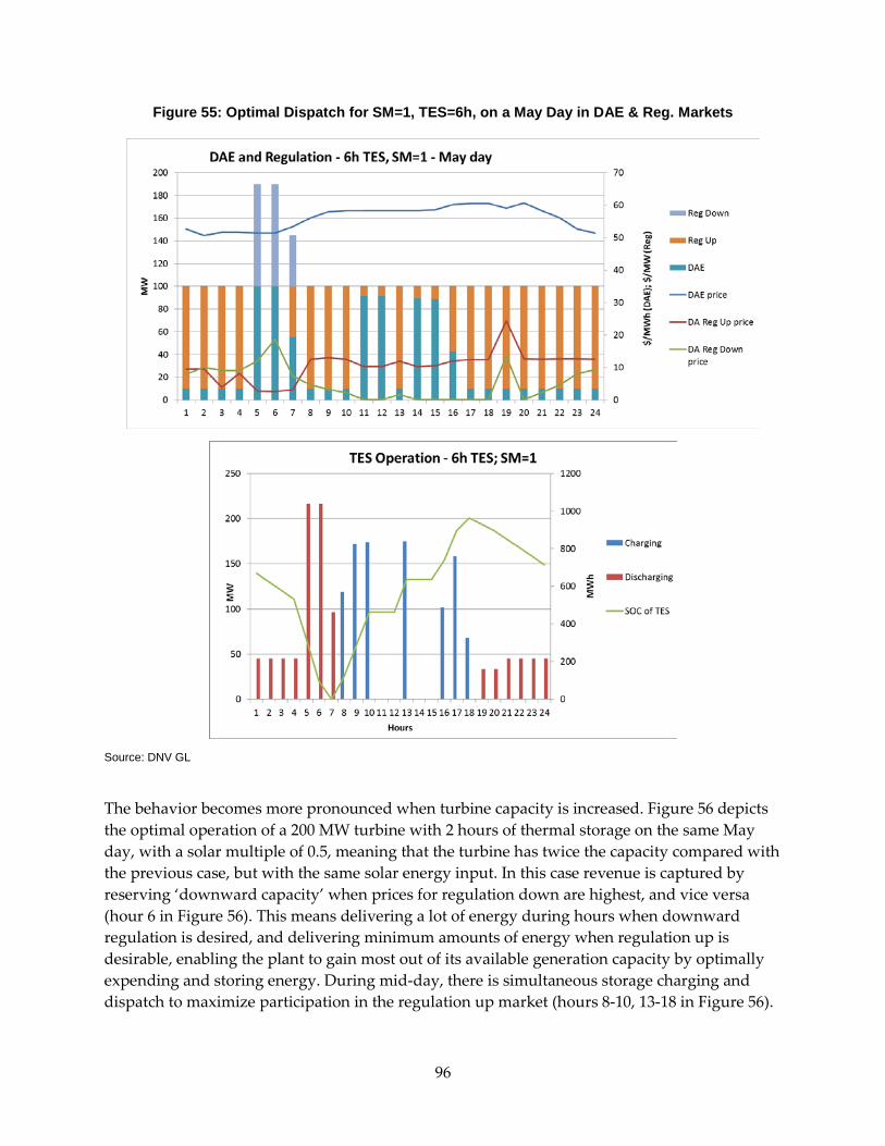
Figure 55: Optimal Dispatch for SM=1, TES=6h, on a May Day in DAE & Reg. Markets
Source: DNV GL
The behavior becomes more pronounced when turbine capacity is increased. Figure 56 depicts the optimal operation of a 200 MW turbine with 2 hours of thermal storage on the same May day, with a solar multiple of 0.5, meaning that the turbine has twice the capacity compared with the previous case, but with the same solar energy input. In this case revenue is captured by reserving ‘downward capacity’ when prices for regulation down are highest, and vice versa (hour 6 in Figure 56). This means delivering a lot of energy during hours when downward regulation is desired, and delivering minimum amounts of energy when regulation up is desirable, enabling the plant to gain most out of its available generation capacity by optimally expending and storing energy. During mid-day, there is simultaneous storage charging and dispatch to maximize participation in the regulation up market (hours 8-10, 13-18 in Figure 56).
96
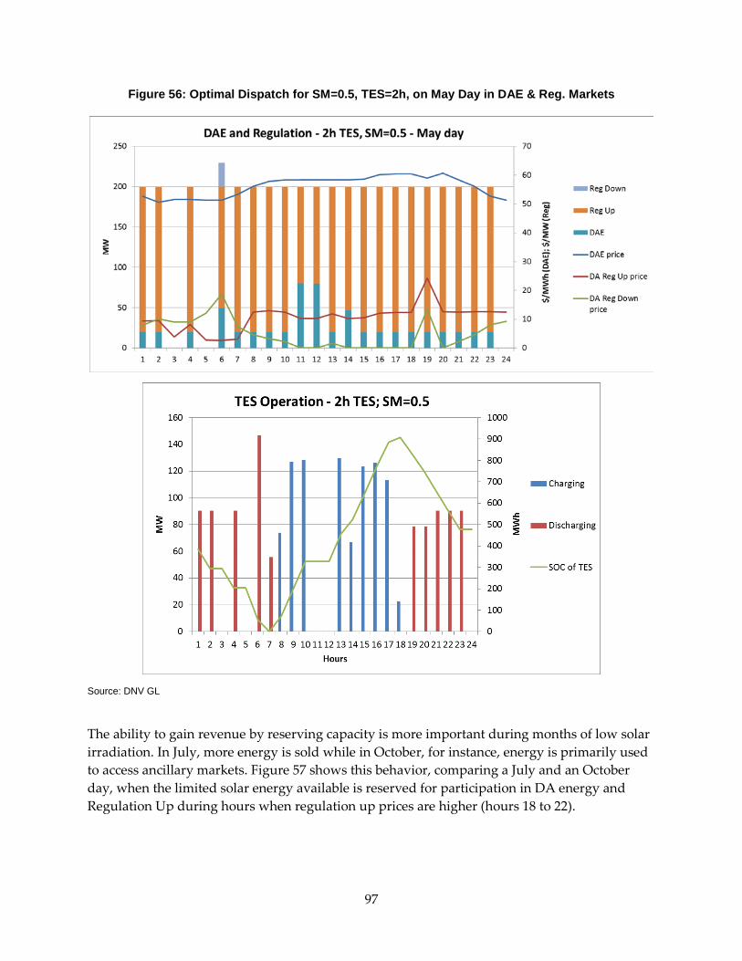
Figure 56: Optimal Dispatch for SM=0.5, TES=2h, on May Day in DAE & Reg. Markets
Source: DNV GL
The ability to gain revenue by reserving capacity is more important during months of low solar irradiation. In July, more energy is sold while in October, for instance, energy is primarily used to access ancillary markets. Figure 57 shows this behavior, comparing a July and an October day, when the limited solar energy available is reserved for participation in DA energy and Regulation Up during hours when regulation up prices are higher (hours 18 to 22).
97
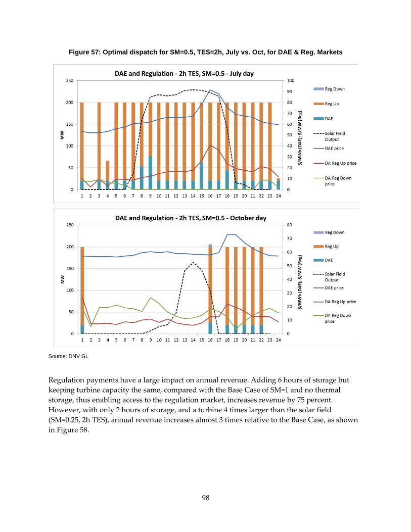
Figure 57: Optimal dispatch for SM=0.5, TES=2h, July vs. Oct, for DAE & Reg. Markets
Source: DNV GL
Regulation payments have a large impact on annual revenue. Adding 6 hours of storage but keeping turbine capacity the same, compared with the Base Case of SM=1 and no thermal storage, thus enabling access to the regulation market, increases revenue by 75 percent. However, with only 2 hours of storage, and a turbine 4 times larger than the solar field (SM=0.25, 2h TES), annual revenue increases almost 3 times relative to the Base Case, as shown in Figure 58.
98
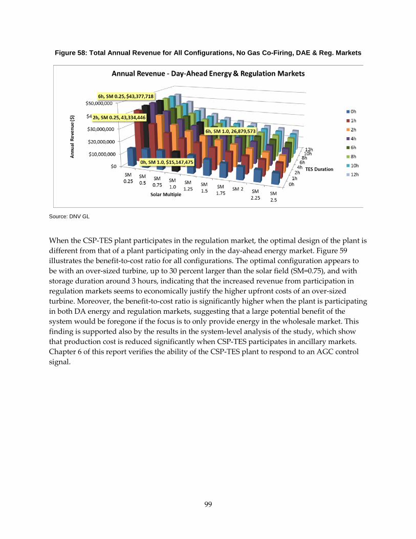
Figure 58: Total Annual Revenue for All Configurations, No Gas Co-Firing, DAE & Reg. Markets
Source: DNV GL
When the CSP-TES plant participates in the regulation market, the optimal design of the plant is different from that of a plant participating only in the day-ahead energy market. Figure 59 illustrates the benefit-to-cost ratio for all configurations. The optimal configuration appears to be with an over-sized turbine, up to 30 percent larger than the solar field (SM=0.75), and with storage duration around 3 hours, indicating that the increased revenue from participation in regulation markets seems to economically justify the higher upfront costs of an over-sized turbine. Moreover, the benefit-to-cost ratio is significantly higher when the plant is participating in both DA energy and regulation markets, suggesting that a large potential benefit of the system would be foregone if the focus is to only provide energy in the wholesale market. This finding is supported also by the results in the system-level analysis of the study, which show that production cost is reduced significantly when CSP-TES participates in ancillary markets. Chapter 6 of this report verifies the ability of the CSP-TES plant to respond to an AGC control signal.
99
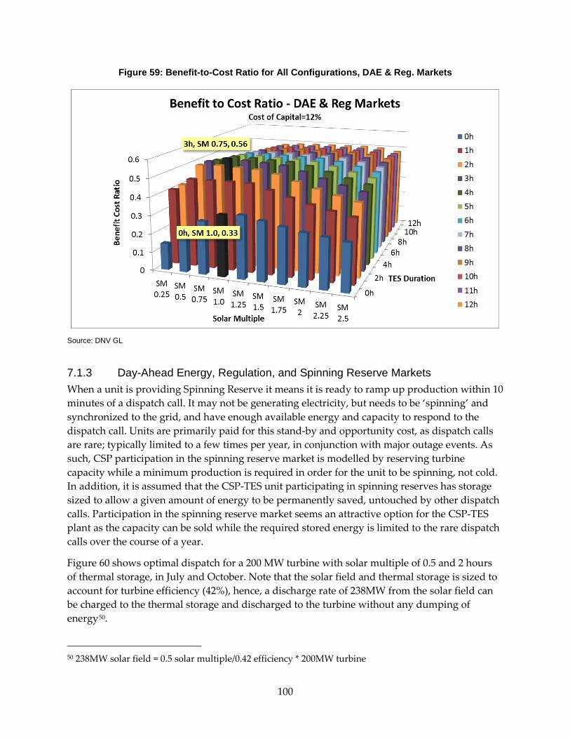
Figure 59: Benefit-to-Cost Ratio for All Configurations, DAE & Reg. Markets
Source: DNV GL
7.1.3 Day-Ahead Energy, Regulation, and Spinning Reserve Markets When a unit is providing Spinning Reserve it means it is ready to ramp up production within 10 minutes of a dispatch call. It may not be generating electricity, but needs to be ‘spinning’ and synchronized to the grid, and have enough available energy and capacity to respond to the dispatch call. Units are primarily paid for this stand-by and opportunity cost, as dispatch calls are rare; typically limited to a few times per year, in conjunction with major outage events. As such, CSP participation in the spinning reserve market is modelled by reserving turbine capacity while a minimum production is required in order for the unit to be spinning, not cold. In addition, it is assumed that the CSP-TES unit participating in spinning reserves has storage sized to allow a given amount of energy to be permanently saved, untouched by other dispatch calls. Participation in the spinning reserve market seems an attractive option for the CSP-TES plant as the capacity can be sold while the required stored energy is limited to the rare dispatch calls over the course of a year.
Figure 60 shows optimal dispatch for a 200 MW turbine with solar multiple of 0.5 and 2 hours of thermal storage, in July and October. Note that the solar field and thermal storage is sized to account for turbine efficiency (42%), hence, a discharge rate of 238MW from the solar field can be charged to the thermal storage and discharged to the turbine without any dumping of energy50.
50 238MW solar field = 0.5 solar multiple/0.42 efficiency * 200MW turbine
100
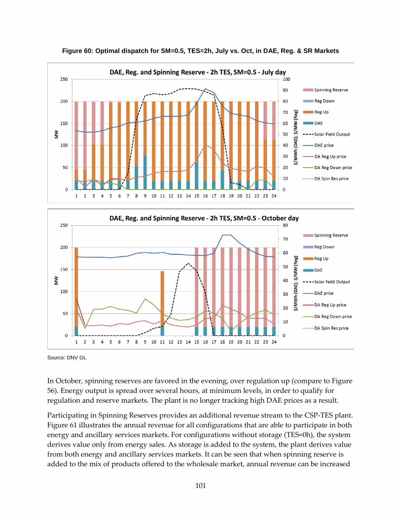
Figure 60: Optimal dispatch for SM=0.5, TES=2h, July vs. Oct, in DAE, Reg. & SR Markets
Source: DNV GL
In October, spinning reserves are favored in the evening, over regulation up (compare to Figure 56). Energy output is spread over several hours, at minimum levels, in order to qualify for regulation and reserve markets. The plant is no longer tracking high DAE prices as a result.
Participating in Spinning Reserves provides an additional revenue stream to the CSP-TES plant. Figure 61 illustrates the annual revenue for all configurations that are able to participate in both energy and ancillary services markets. For configurations without storage (TES=0h), the system derives value only from energy sales. As storage is added to the system, the plant derives value from both energy and ancillary services markets. It can be seen that when spinning reserve is added to the mix of products offered to the wholesale market, annual revenue can be increased
101
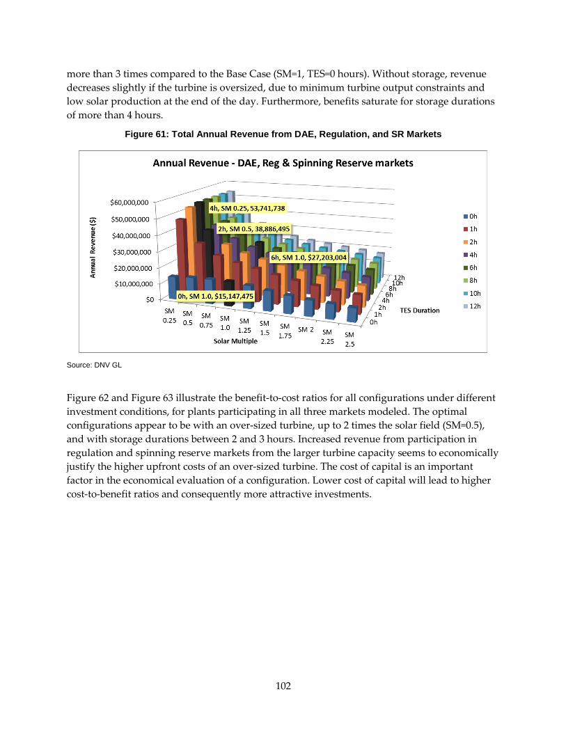
more than 3 times compared to the Base Case (SM=1, TES=0 hours). Without storage, revenue decreases slightly if the turbine is oversized, due to minimum turbine output constraints and low solar production at the end of the day. Furthermore, benefits saturate for storage durations of more than 4 hours.
Figure 61: Total Annual Revenue from DAE, Regulation, and SR Markets
Source: DNV GL
Figure 62 and Figure 63 illustrate the benefit-to-cost ratios for all configurations under different investment conditions, for plants participating in all three markets modeled. The optimal configurations appear to be with an over-sized turbine, up to 2 times the solar field (SM=0.5), and with storage durations between 2 and 3 hours. Increased revenue from participation in regulation and spinning reserve markets from the larger turbine capacity seems to economically justify the higher upfront costs of an over-sized turbine. The cost of capital is an important factor in the economical evaluation of a configuration. Lower cost of capital will lead to higher cost-to-benefit ratios and consequently more attractive investments.
102
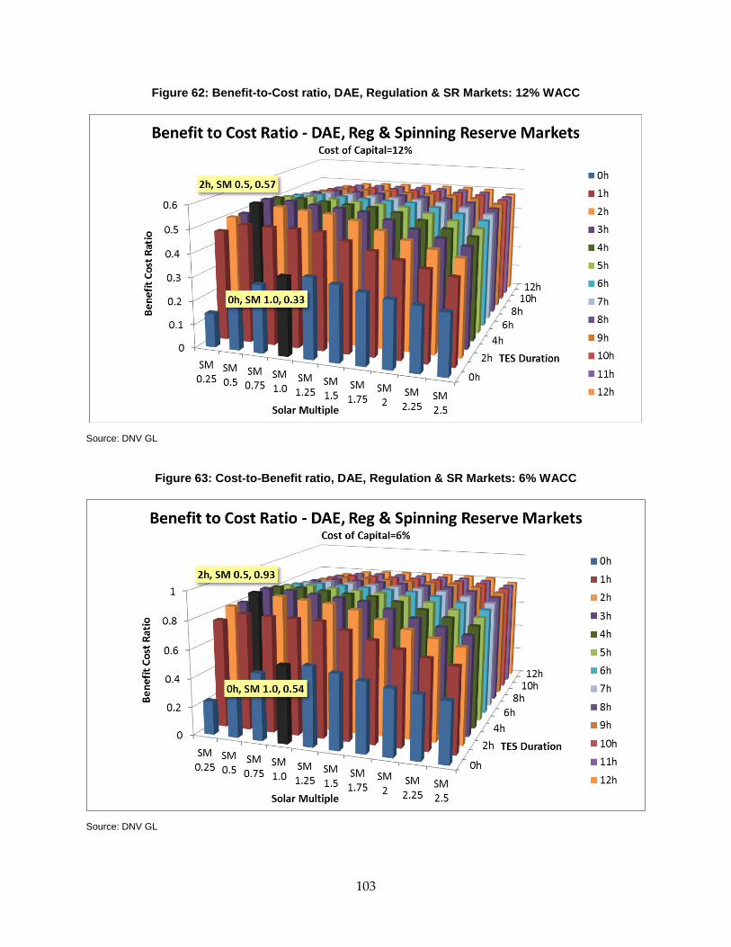
Figure 62: Benefit-to-Cost ratio, DAE, Regulation & SR Markets: 12% WACC
Source: DNV GL
Figure 63: Cost-to-Benefit ratio, DAE, Regulation & SR Markets: 6% WACC
Source: DNV GL
103
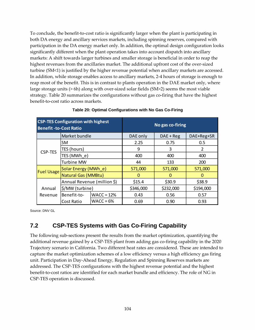
To conclude, the benefit-to-cost ratio is significantly larger when the plant is participating in both DA energy and ancillary services markets, including spinning reserves, compared with participation in the DA energy market only. In addition, the optimal design configuration looks significantly different when the plant operation takes into account dispatch into ancillary markets: A shift towards larger turbines and smaller storage is beneficial in order to reap the highest revenues from the ancillaries market. The additional upfront cost of the over-sized turbine (SM<1) is justified by the higher revenue potential when ancillary markets are accessed. In addition, while storage enables access to ancillary markets, 2-4 hours of storage is enough to reap most of the benefit. This is in contrast to plants operation in the DAE market only, where large storage units (> 6h) along with over-sized solar fields (SM>2) seems the most viable strategy. Table 20 summarizes the configurations without gas co-firing that have the highest benefit-to-cost ratio across markets.
Table 20: Optimal Configurations with No Gas Co-Firing
Source: DNV GL
7.2 CSP-TES Systems with Gas Co-Firing Capability The following sub-sections present the results from the market optimization, quantifying the additional revenue gained by a CSP-TES plant from adding gas co-firing capability in the 2020 Trajectory scenario in California. Two different heat rates are considered. These are intended to capture the market optimization schemes of a low efficiency versus a high efficiency gas firing unit. Participation in Day-Ahead Energy, Regulation and Spinning Reserves markets are addressed. The CSP-TES configurations with the highest revenue potential and the highest benefit-to-cost ratios are identified for each market bundle and efficiency. The role of NG in CSP-TES operation is discussed.
Market bundle DAE only DAE + Reg DAE+Reg+SR2.25 0.75 0.5
9 3 2400 400 40044 133 200
571,000 571,000 571,0000 0 0
$15.4 $30.9 $38.9$346,000 $232,000 $194,000
WACC = 12% 0.43 0.56 0.57WACC = 6% 0.69 0.90 0.93
CSP-TES Configuration with highest Benefit -to-Cost Ratio
No gas co-firing
CSP-TES
SMTES (hours)TES (MWh_e)Turbine MW
Fuel Usage Solar Energy (MWh_e)Natural Gas (MMBtu)
Annual Revenue
Annual Revenue (million $)$/MW (turbine)Benefit-to-Cost Ratio
104
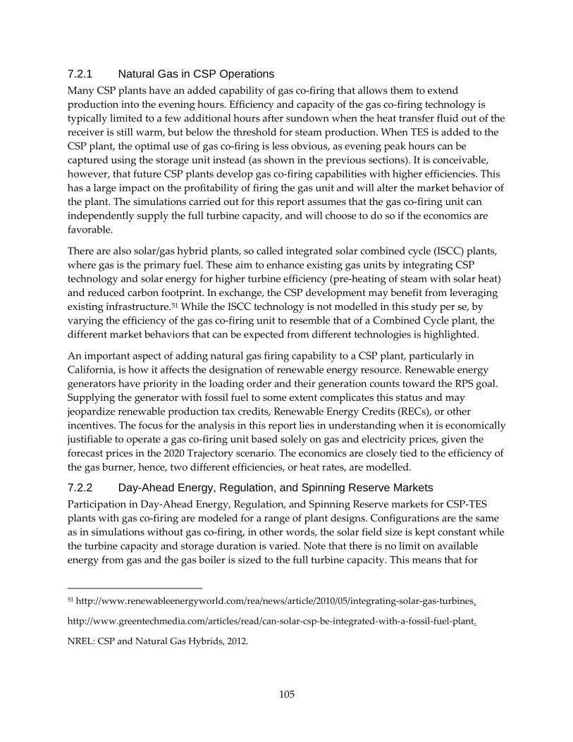
7.2.1 Natural Gas in CSP Operations Many CSP plants have an added capability of gas co-firing that allows them to extend production into the evening hours. Efficiency and capacity of the gas co-firing technology is typically limited to a few additional hours after sundown when the heat transfer fluid out of the receiver is still warm, but below the threshold for steam production. When TES is added to the CSP plant, the optimal use of gas co-firing is less obvious, as evening peak hours can be captured using the storage unit instead (as shown in the previous sections). It is conceivable, however, that future CSP plants develop gas co-firing capabilities with higher efficiencies. This has a large impact on the profitability of firing the gas unit and will alter the market behavior of the plant. The simulations carried out for this report assumes that the gas co-firing unit can independently supply the full turbine capacity, and will choose to do so if the economics are favorable.
There are also solar/gas hybrid plants, so called integrated solar combined cycle (ISCC) plants, where gas is the primary fuel. These aim to enhance existing gas units by integrating CSP technology and solar energy for higher turbine efficiency (pre-heating of steam with solar heat) and reduced carbon footprint. In exchange, the CSP development may benefit from leveraging existing infrastructure.51 While the ISCC technology is not modelled in this study per se, by varying the efficiency of the gas co-firing unit to resemble that of a Combined Cycle plant, the different market behaviors that can be expected from different technologies is highlighted.
An important aspect of adding natural gas firing capability to a CSP plant, particularly in California, is how it affects the designation of renewable energy resource. Renewable energy generators have priority in the loading order and their generation counts toward the RPS goal. Supplying the generator with fossil fuel to some extent complicates this status and may jeopardize renewable production tax credits, Renewable Energy Credits (RECs), or other incentives. The focus for the analysis in this report lies in understanding when it is economically justifiable to operate a gas co-firing unit based solely on gas and electricity prices, given the forecast prices in the 2020 Trajectory scenario. The economics are closely tied to the efficiency of the gas burner, hence, two different efficiencies, or heat rates, are modelled.
7.2.2 Day-Ahead Energy, Regulation, and Spinning Reserve Markets Participation in Day-Ahead Energy, Regulation, and Spinning Reserve markets for CSP-TES plants with gas co-firing are modeled for a range of plant designs. Configurations are the same as in simulations without gas co-firing, in other words, the solar field size is kept constant while the turbine capacity and storage duration is varied. Note that there is no limit on available energy from gas and the gas boiler is sized to the full turbine capacity. This means that for
51 http://www.renewableenergyworld.com/rea/news/article/2010/05/integrating-solar-gas-turbines.
http://www.greentechmedia.com/articles/read/can-solar-csp-be-integrated-with-a-fossil-fuel-plant.
NREL: CSP and Natural Gas Hybrids, 2012.
105
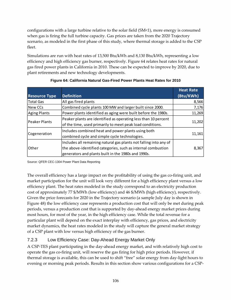
configurations with a large turbine relative to the solar field (SM<1), more energy is consumed when gas is firing the full turbine capacity. Gas prices are taken from the 2020 Trajectory scenario, as modeled in the first phase of this study, where thermal storage is added to the CSP fleet.
Simulations are run with heat rates of 13,500 Btu/kWh and 8,130 Btu/kWh, representing a low efficiency and high efficiency gas burner, respectively. Figure 64 relates heat rates for natural gas fired power plants in California in 2010. These can be expected to improve by 2020, due to plant retirements and new technology developments.
Figure 64: California Natural Gas-Fired Power Plants Heat Rates for 2010
Source: QFER CEC-1304 Power Plant Data Reporting
The overall efficiency has a large impact on the profitability of using the gas co-firing unit, and market participation for the unit will look very different for a high efficiency plant versus a low efficiency plant. The heat rates modeled in the study correspond to an electricity production cost of approximately 77 $/MWh (low efficiency) and 46 $/MWh (high efficiency), respectively. Given the price forecasts for 2020 in the Trajectory scenario (a sample July day is shown in Figure 48) the low efficiency case represents a production cost that will only be met during peak periods, versus a production cost that is supported by day-ahead energy market prices during most hours, for most of the year, in the high efficiency case. While the total revenue for a particular plant will depend on the exact interplay with efficiency, gas prices, and electricity market dynamics, the heat rates modeled in the study will capture the general market strategy of a CSP plant with low versus high efficiency of the gas burner.
7.2.3 Low Efficiency Case: Day-Ahead Energy Market Only A CSP-TES plant participating in the day-ahead energy market, and with relatively high cost to operate the gas co-firing unit, will reserve the gas firing for high price periods. However, if thermal storage is available, this can be used to shift “free” solar energy from day-light hours to evening or morning peak periods. Results in this section show various configurations for a CSP-
Resource Type DefinitionHeat Rate
(Btu/KWh)Total Gas All gas fired plants 8,566New CCs Combined cycle plants 100 MW and larger built since 2000. 7,176Aging Plants Power plants identified as aging were built before the 1980s. 11,269
Peaker PlantsPeaker plants are identified as operating less than 10 percent of the time, used primarily to meet peak load conditions.
11,202
CogenerationIncludes combined heat and power plants using both combined cycle and simple cycle technologies.
11,161
OtherIncludes all remaining natural gas plants not falling into any of the above-identified categories, such as internal combustion generators and plants built in the 1980s and 1990s.
8,367
106
TES plant with a heat rate of 13,500 Btu/kWh, equivalent to a production cost for gas of approximately 77 $/MWh,
7.2.3.1 Optimal Dispatch without Storage Figure 65 and Figure 66 show the optimal dispatch, meaning the market participation that gives the highest revenue, for a CSP plant without storage, and with low gas burning efficiency. The production cost for gas (approximately 77 $/MWh) is also marked in the figures along with the DAE price curve for a July and a November day, respectively. In addition, the figures show which portion of the turbine output comes from the solar field versus the gas burner.
In summer (Figure 65), gas is used sparingly as the turbine capacity (even without storage) is committed almost fully with solar energy. Note that in hours 19-20 on this July day, gas is used to reach turbine minimum output levels (10 percent of total capacity for these simulations), despite a DAE price below the cost of production. Without gas co-firing, this solar energy would be wasted, as the heat input is not enough to drive the turbine and no storage is available to capture the energy. With the solar and gas combined, the plant still benefits from producing at this price.
In winter months (Figure 66) with low solar input, gas is used to take advantage of peak prices. Note again in hour 9 how gas is used to reach minimum turbine output levels.
Figure 65: Optimal Dispatch on July Day in DAE Market: Low Efficiency, No Storage
Source: DNV GL
107
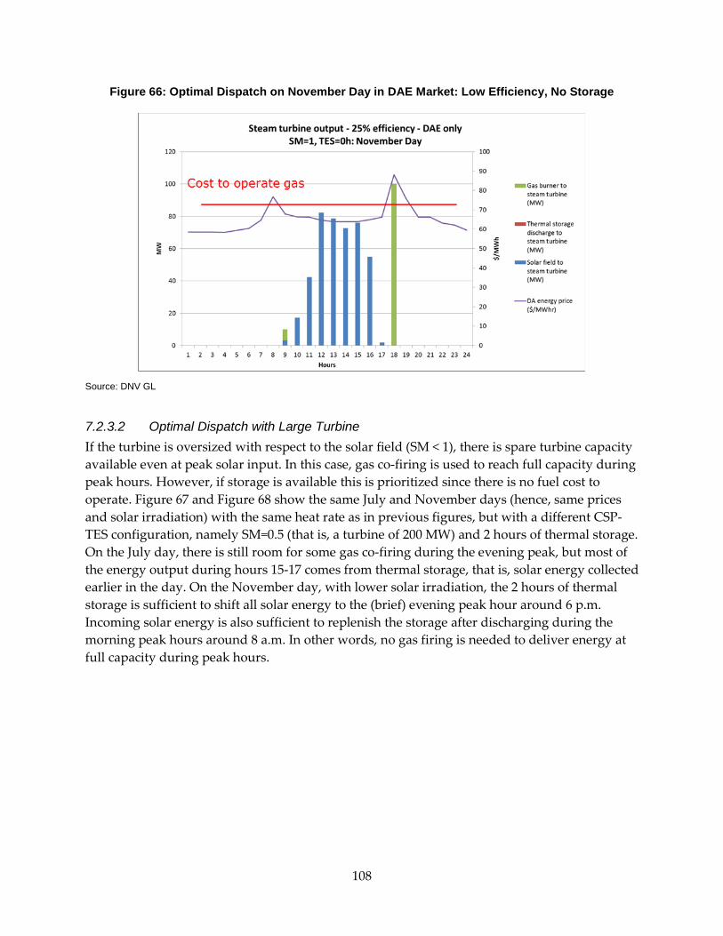
Figure 66: Optimal Dispatch on November Day in DAE Market: Low Efficiency, No Storage
Source: DNV GL
7.2.3.2 Optimal Dispatch with Large Turbine If the turbine is oversized with respect to the solar field (SM < 1), there is spare turbine capacity available even at peak solar input. In this case, gas co-firing is used to reach full capacity during peak hours. However, if storage is available this is prioritized since there is no fuel cost to operate. Figure 67 and Figure 68 show the same July and November days (hence, same prices and solar irradiation) with the same heat rate as in previous figures, but with a different CSP-TES configuration, namely SM=0.5 (that is, a turbine of 200 MW) and 2 hours of thermal storage. On the July day, there is still room for some gas co-firing during the evening peak, but most of the energy output during hours 15-17 comes from thermal storage, that is, solar energy collected earlier in the day. On the November day, with lower solar irradiation, the 2 hours of thermal storage is sufficient to shift all solar energy to the (brief) evening peak hour around 6 p.m. Incoming solar energy is also sufficient to replenish the storage after discharging during the morning peak hours around 8 a.m. In other words, no gas firing is needed to deliver energy at full capacity during peak hours.
108
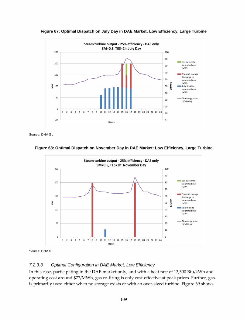
Figure 67: Optimal Dispatch on July Day in DAE Market: Low Efficiency, Large Turbine
Source: DNV GL
Figure 68: Optimal Dispatch on November Day in DAE Market: Low Efficiency, Large Turbine
Source: DNV GL
7.2.3.3 Optimal Configuration in DAE Market, Low Efficiency In this case, participating in the DAE market only, and with a heat rate of 13,500 Btu/kWh and operating cost around $77/MWh, gas co-firing is only cost-effective at peak prices. Further, gas is primarily used either when no storage exists or with an over-sized turbine. Figure 69 shows
109
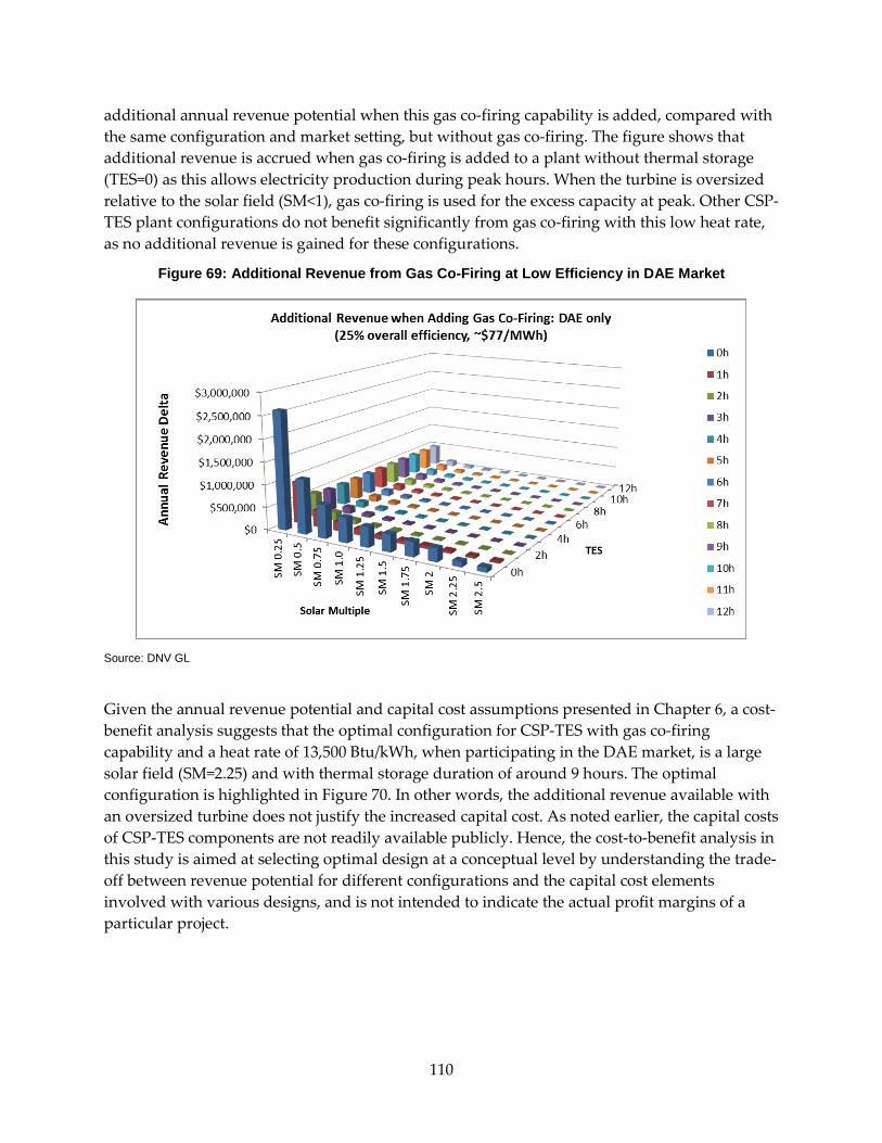
additional annual revenue potential when this gas co-firing capability is added, compared with the same configuration and market setting, but without gas co-firing. The figure shows that additional revenue is accrued when gas co-firing is added to a plant without thermal storage (TES=0) as this allows electricity production during peak hours. When the turbine is oversized relative to the solar field (SM<1), gas co-firing is used for the excess capacity at peak. Other CSP-TES plant configurations do not benefit significantly from gas co-firing with this low heat rate, as no additional revenue is gained for these configurations.
Figure 69: Additional Revenue from Gas Co-Firing at Low Efficiency in DAE Market
Source: DNV GL
Given the annual revenue potential and capital cost assumptions presented in Chapter 6, a cost-benefit analysis suggests that the optimal configuration for CSP-TES with gas co-firing capability and a heat rate of 13,500 Btu/kWh, when participating in the DAE market, is a large solar field (SM=2.25) and with thermal storage duration of around 9 hours. The optimal configuration is highlighted in Figure 70. In other words, the additional revenue available with an oversized turbine does not justify the increased capital cost. As noted earlier, the capital costs of CSP-TES components are not readily available publicly. Hence, the cost-to-benefit analysis in this study is aimed at selecting optimal design at a conceptual level by understanding the trade-off between revenue potential for different configurations and the capital cost elements involved with various designs, and is not intended to indicate the actual profit margins of a particular project.
110
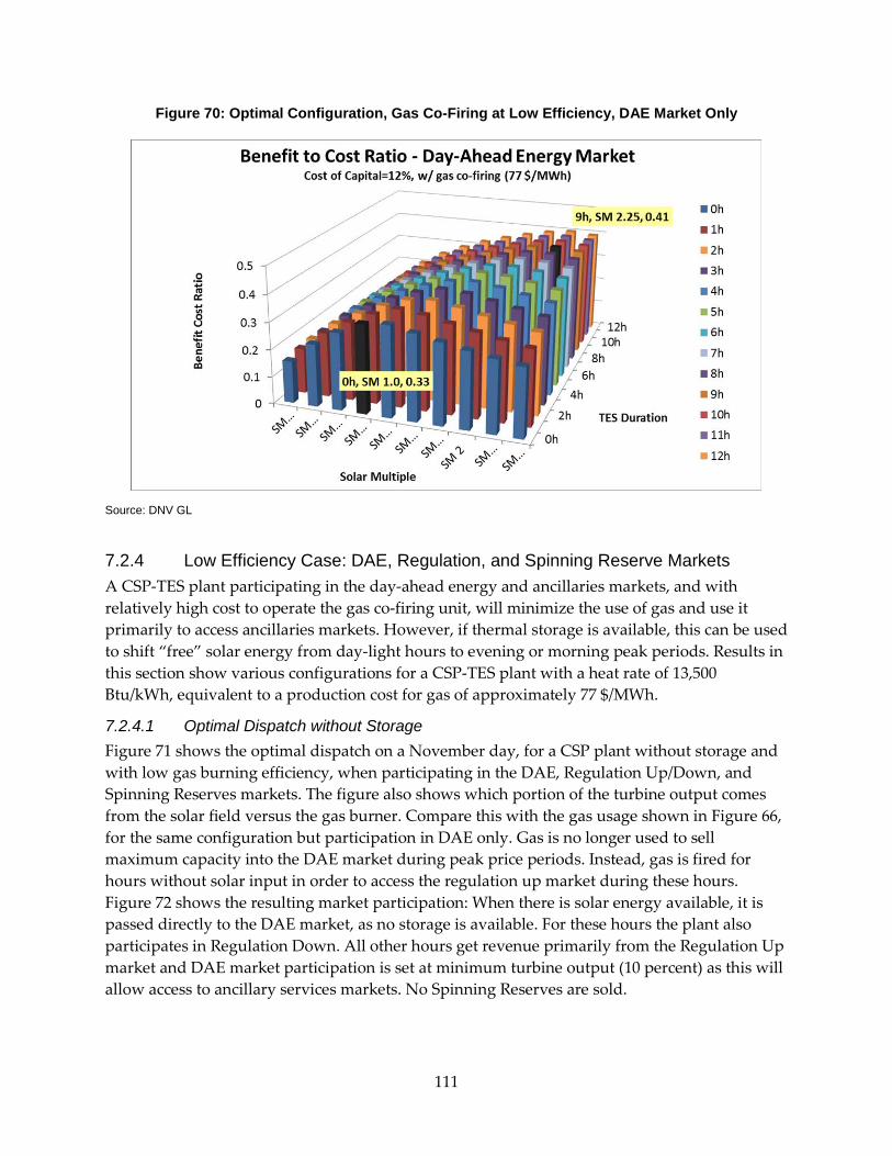
Figure 70: Optimal Configuration, Gas Co-Firing at Low Efficiency, DAE Market Only
Source: DNV GL
7.2.4 Low Efficiency Case: DAE, Regulation, and Spinning Reserve Markets A CSP-TES plant participating in the day-ahead energy and ancillaries markets, and with relatively high cost to operate the gas co-firing unit, will minimize the use of gas and use it primarily to access ancillaries markets. However, if thermal storage is available, this can be used to shift “free” solar energy from day-light hours to evening or morning peak periods. Results in this section show various configurations for a CSP-TES plant with a heat rate of 13,500 Btu/kWh, equivalent to a production cost for gas of approximately 77 $/MWh.
7.2.4.1 Optimal Dispatch without Storage Figure 71 shows the optimal dispatch on a November day, for a CSP plant without storage and with low gas burning efficiency, when participating in the DAE, Regulation Up/Down, and Spinning Reserves markets. The figure also shows which portion of the turbine output comes from the solar field versus the gas burner. Compare this with the gas usage shown in Figure 66, for the same configuration but participation in DAE only. Gas is no longer used to sell maximum capacity into the DAE market during peak price periods. Instead, gas is fired for hours without solar input in order to access the regulation up market during these hours. Figure 72 shows the resulting market participation: When there is solar energy available, it is passed directly to the DAE market, as no storage is available. For these hours the plant also participates in Regulation Down. All other hours get revenue primarily from the Regulation Up market and DAE market participation is set at minimum turbine output (10 percent) as this will allow access to ancillary services markets. No Spinning Reserves are sold.
111
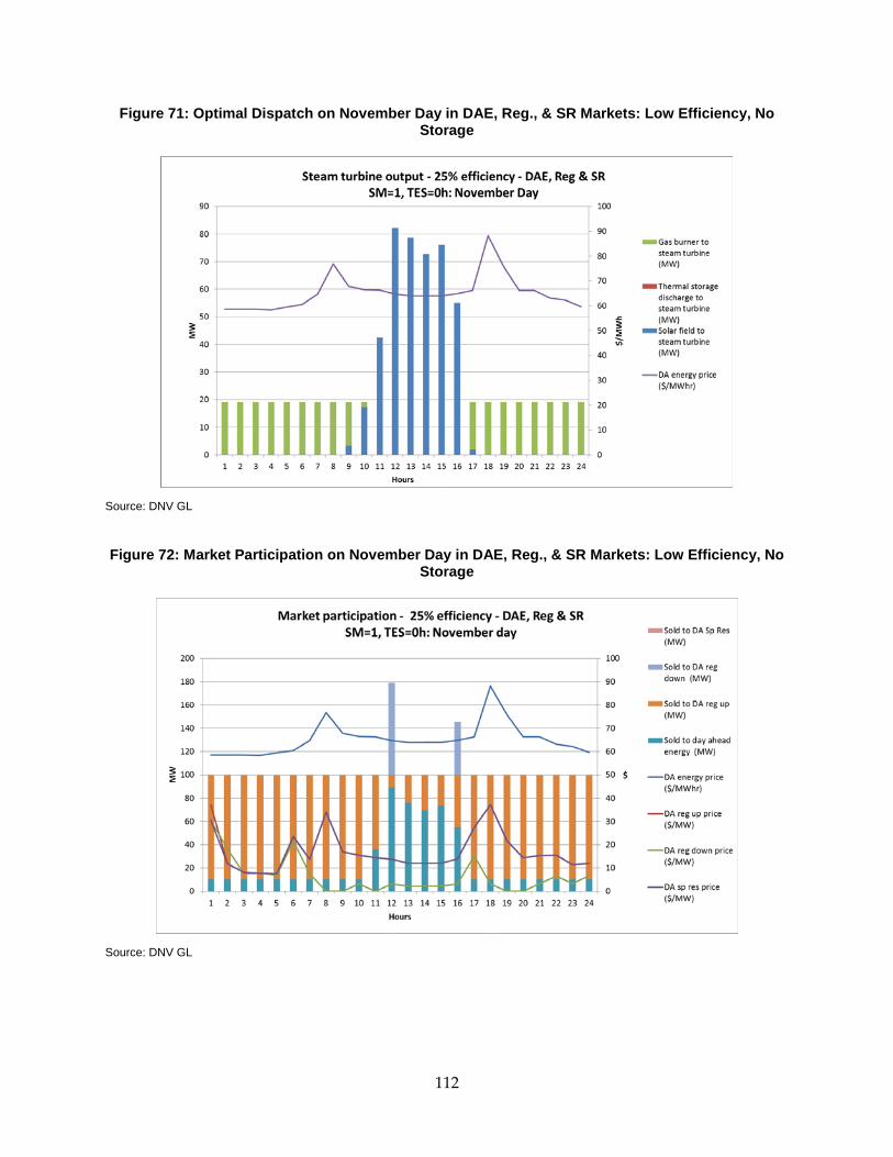
Figure 71: Optimal Dispatch on November Day in DAE, Reg., & SR Markets: Low Efficiency, No Storage
Source: DNV GL
Figure 72: Market Participation on November Day in DAE, Reg., & SR Markets: Low Efficiency, No Storage
Source: DNV GL
112
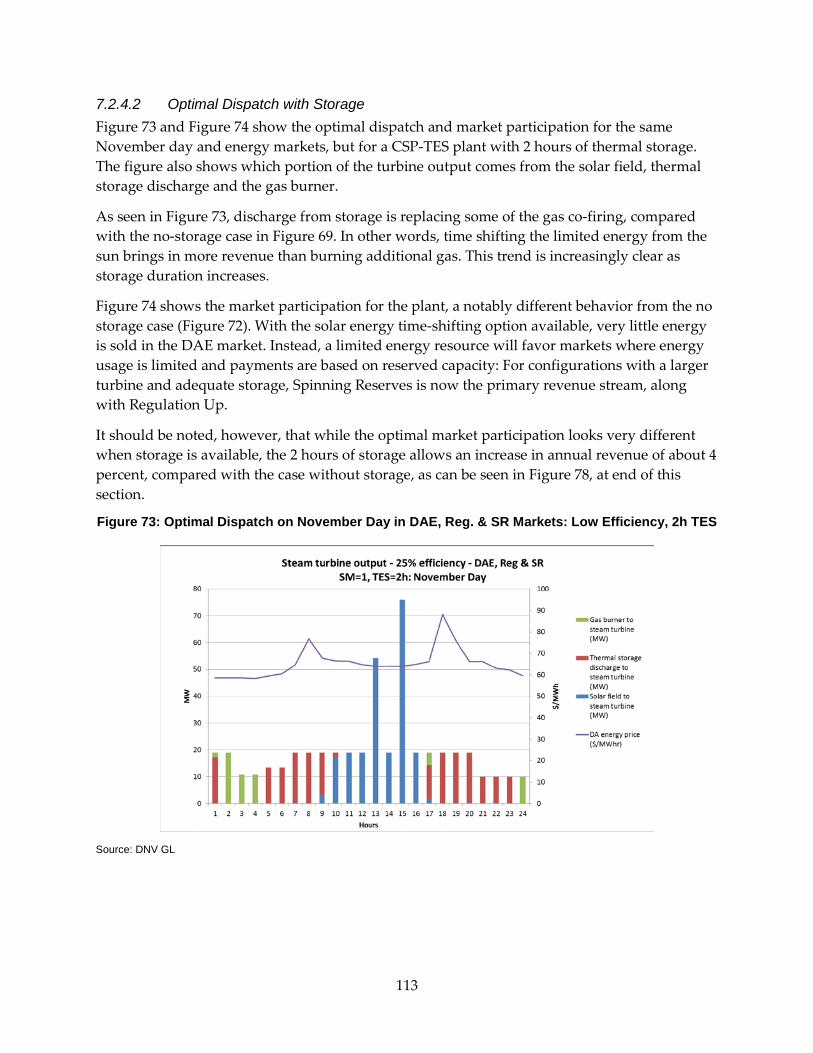
7.2.4.2 Optimal Dispatch with Storage Figure 73 and Figure 74 show the optimal dispatch and market participation for the same November day and energy markets, but for a CSP-TES plant with 2 hours of thermal storage. The figure also shows which portion of the turbine output comes from the solar field, thermal storage discharge and the gas burner.
As seen in Figure 73, discharge from storage is replacing some of the gas co-firing, compared with the no-storage case in Figure 69. In other words, time shifting the limited energy from the sun brings in more revenue than burning additional gas. This trend is increasingly clear as storage duration increases.
Figure 74 shows the market participation for the plant, a notably different behavior from the no storage case (Figure 72). With the solar energy time-shifting option available, very little energy is sold in the DAE market. Instead, a limited energy resource will favor markets where energy usage is limited and payments are based on reserved capacity: For configurations with a larger turbine and adequate storage, Spinning Reserves is now the primary revenue stream, along with Regulation Up.
It should be noted, however, that while the optimal market participation looks very different when storage is available, the 2 hours of storage allows an increase in annual revenue of about 4 percent, compared with the case without storage, as can be seen in Figure 78, at end of this section.
Figure 73: Optimal Dispatch on November Day in DAE, Reg. & SR Markets: Low Efficiency, 2h TES
Source: DNV GL
113
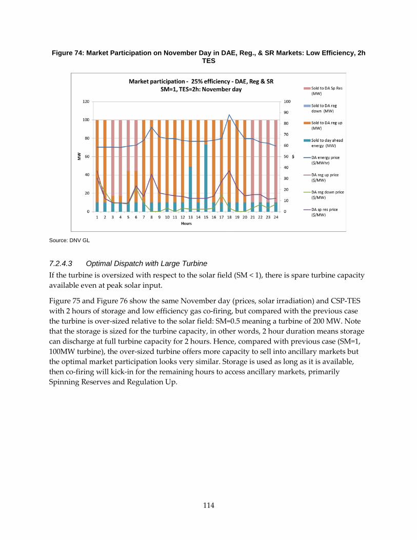
Figure 74: Market Participation on November Day in DAE, Reg., & SR Markets: Low Efficiency, 2h TES
Source: DNV GL
7.2.4.3 Optimal Dispatch with Large Turbine If the turbine is oversized with respect to the solar field (SM < 1), there is spare turbine capacity available even at peak solar input.
Figure 75 and Figure 76 show the same November day (prices, solar irradiation) and CSP-TES with 2 hours of storage and low efficiency gas co-firing, but compared with the previous case the turbine is over-sized relative to the solar field: SM=0.5 meaning a turbine of 200 MW. Note that the storage is sized for the turbine capacity, in other words, 2 hour duration means storage can discharge at full turbine capacity for 2 hours. Hence, compared with previous case (SM=1, 100MW turbine), the over-sized turbine offers more capacity to sell into ancillary markets but the optimal market participation looks very similar. Storage is used as long as it is available, then co-firing will kick-in for the remaining hours to access ancillary markets, primarily Spinning Reserves and Regulation Up.
114
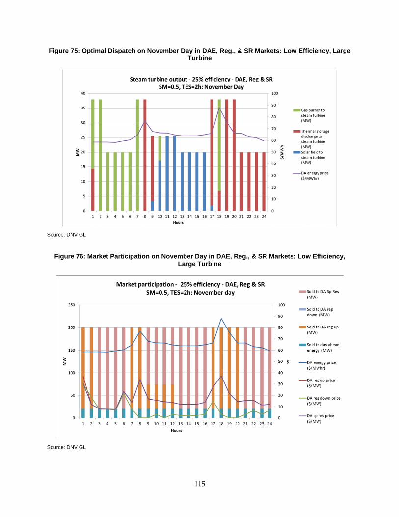
Figure 75: Optimal Dispatch on November Day in DAE, Reg., & SR Markets: Low Efficiency, Large Turbine
Source: DNV GL
Figure 76: Market Participation on November Day in DAE, Reg., & SR Markets: Low Efficiency, Large Turbine
Source: DNV GL
115
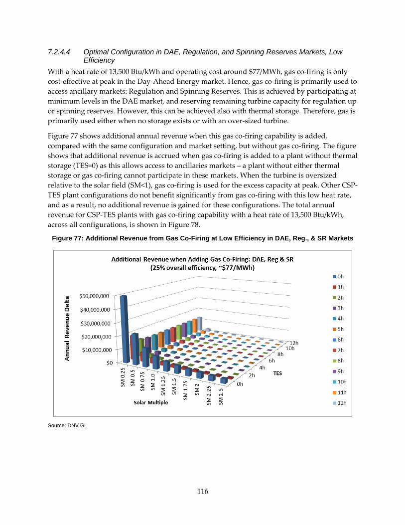
7.2.4.4 Optimal Configuration in DAE, Regulation, and Spinning Reserves Markets, Low Efficiency
With a heat rate of 13,500 Btu/kWh and operating cost around $77/MWh, gas co-firing is only cost-effective at peak in the Day-Ahead Energy market. Hence, gas co-firing is primarily used to access ancillary markets: Regulation and Spinning Reserves. This is achieved by participating at minimum levels in the DAE market, and reserving remaining turbine capacity for regulation up or spinning reserves. However, this can be achieved also with thermal storage. Therefore, gas is primarily used either when no storage exists or with an over-sized turbine.
Figure 77 shows additional annual revenue when this gas co-firing capability is added, compared with the same configuration and market setting, but without gas co-firing. The figure shows that additional revenue is accrued when gas co-firing is added to a plant without thermal storage (TES=0) as this allows access to ancillaries markets – a plant without either thermal storage or gas co-firing cannot participate in these markets. When the turbine is oversized relative to the solar field (SM<1), gas co-firing is used for the excess capacity at peak. Other CSP-TES plant configurations do not benefit significantly from gas co-firing with this low heat rate, and as a result, no additional revenue is gained for these configurations. The total annual revenue for CSP-TES plants with gas co-firing capability with a heat rate of 13,500 Btu/kWh, across all configurations, is shown in Figure 78.
Figure 77: Additional Revenue from Gas Co-Firing at Low Efficiency in DAE, Reg., & SR Markets
Source: DNV GL
116
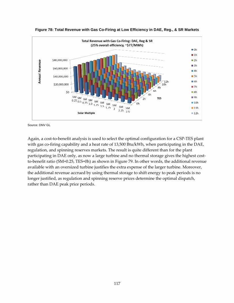
Figure 78: Total Revenue with Gas Co-Firing at Low Efficiency in DAE, Reg., & SR Markets
Source: DNV GL
Again, a cost-to-benefit analysis is used to select the optimal configuration for a CSP-TES plant with gas co-firing capability and a heat rate of 13,500 Btu/kWh, when participating in the DAE, regulation, and spinning reserves markets. The result is quite different than for the plant participating in DAE only, as now a large turbine and no thermal storage gives the highest cost-to-benefit ratio (SM=0.25, TES=0h) as shown in Figure 79. In other words, the additional revenue available with an oversized turbine justifies the extra expense of the larger turbine. Moreover, the additional revenue accrued by using thermal storage to shift energy to peak periods is no longer justified, as regulation and spinning reserve prices determine the optimal dispatch, rather than DAE peak price periods.
117
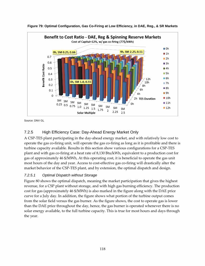
Figure 79: Optimal Configuration, Gas Co-Firing at Low Efficiency, in DAE, Reg., & SR Markets
Source: DNV GL
7.2.5 High Efficiency Case: Day-Ahead Energy Market Only A CSP-TES plant participating in the day-ahead energy market, and with relatively low cost to operate the gas co-firing unit, will operate the gas co-firing as long as it is profitable and there is turbine capacity available. Results in this section show various configurations for a CSP-TES plant and with gas co-firing at a heat rate of 8,130 Btu/kWh, equivalent to a production cost for gas of approximately 46 $/MWh, At this operating cost, it is beneficial to operate the gas unit most hours of the day and year. Access to cost-effective gas co-firing will drastically alter the market behavior of the CSP-TES plant, and by extension, the optimal dispatch and design.
7.2.5.1 Optimal Dispatch without Storage Figure 80 shows the optimal dispatch, meaning the market participation that gives the highest revenue, for a CSP plant without storage, and with high gas burning efficiency. The production cost for gas (approximately 46 $/MWh) is also marked in the figure along with the DAE price curve for a July day. In addition, the figure shows what portion of the turbine output comes from the solar field versus the gas burner. As the figure shows, the cost to operate gas is lower than the DAE price throughout the day, hence, the gas burner is operated whenever there is no solar energy available, to the full turbine capacity. This is true for most hours and days through the year.
118
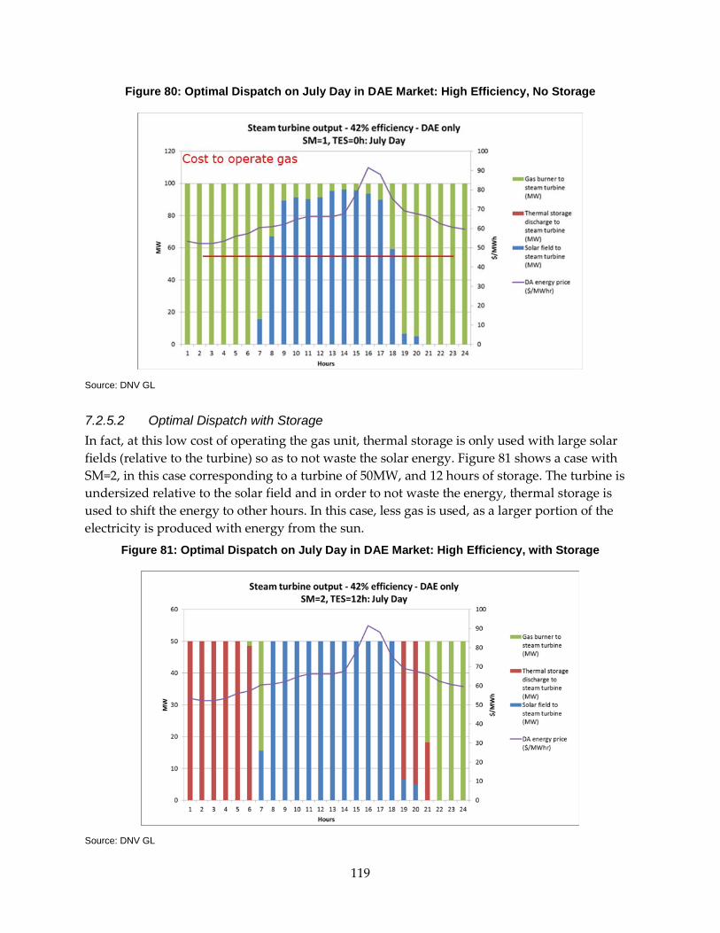
Figure 80: Optimal Dispatch on July Day in DAE Market: High Efficiency, No Storage
Source: DNV GL
7.2.5.2 Optimal Dispatch with Storage In fact, at this low cost of operating the gas unit, thermal storage is only used with large solar fields (relative to the turbine) so as to not waste the solar energy. Figure 81 shows a case with SM=2, in this case corresponding to a turbine of 50MW, and 12 hours of storage. The turbine is undersized relative to the solar field and in order to not waste the energy, thermal storage is used to shift the energy to other hours. In this case, less gas is used, as a larger portion of the electricity is produced with energy from the sun.
Figure 81: Optimal Dispatch on July Day in DAE Market: High Efficiency, with Storage
Source: DNV GL
119
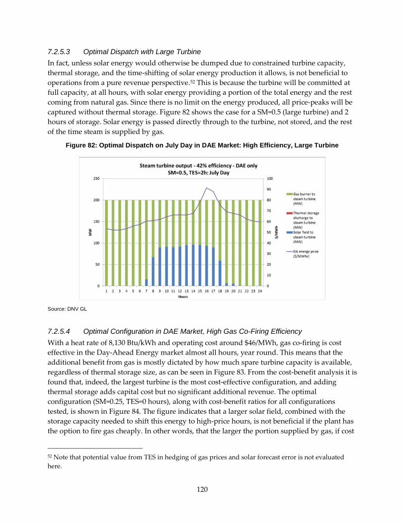
7.2.5.3 Optimal Dispatch with Large Turbine In fact, unless solar energy would otherwise be dumped due to constrained turbine capacity, thermal storage, and the time-shifting of solar energy production it allows, is not beneficial to operations from a pure revenue perspective.52 This is because the turbine will be committed at full capacity, at all hours, with solar energy providing a portion of the total energy and the rest coming from natural gas. Since there is no limit on the energy produced, all price-peaks will be captured without thermal storage. Figure 82 shows the case for a SM=0.5 (large turbine) and 2 hours of storage. Solar energy is passed directly through to the turbine, not stored, and the rest of the time steam is supplied by gas.
Figure 82: Optimal Dispatch on July Day in DAE Market: High Efficiency, Large Turbine
Source: DNV GL
7.2.5.4 Optimal Configuration in DAE Market, High Gas Co-Firing Efficiency With a heat rate of 8,130 Btu/kWh and operating cost around $46/MWh, gas co-firing is cost effective in the Day-Ahead Energy market almost all hours, year round. This means that the additional benefit from gas is mostly dictated by how much spare turbine capacity is available, regardless of thermal storage size, as can be seen in Figure 83. From the cost-benefit analysis it is found that, indeed, the largest turbine is the most cost-effective configuration, and adding thermal storage adds capital cost but no significant additional revenue. The optimal configuration (SM=0.25, TES=0 hours), along with cost-benefit ratios for all configurations tested, is shown in Figure 84. The figure indicates that a larger solar field, combined with the storage capacity needed to shift this energy to high-price hours, is not beneficial if the plant has the option to fire gas cheaply. In other words, that the larger the portion supplied by gas, if cost
52 Note that potential value from TES in hedging of gas prices and solar forecast error is not evaluated here.
120
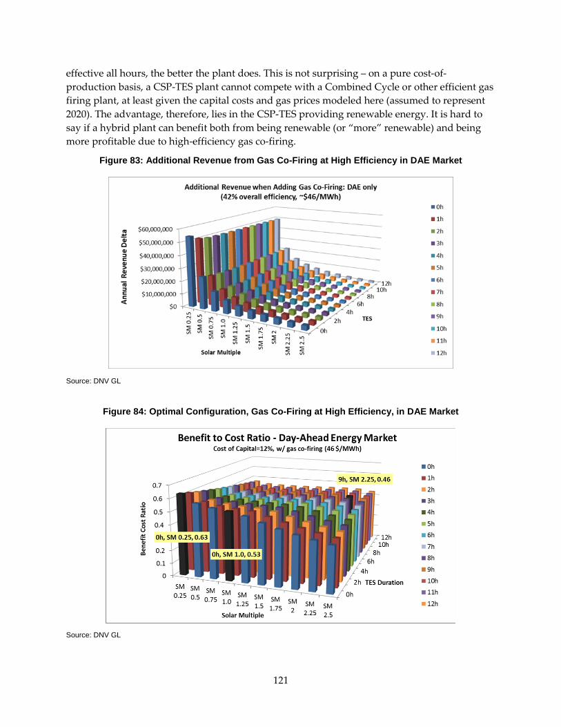
effective all hours, the better the plant does. This is not surprising – on a pure cost-of-production basis, a CSP-TES plant cannot compete with a Combined Cycle or other efficient gas firing plant, at least given the capital costs and gas prices modeled here (assumed to represent 2020). The advantage, therefore, lies in the CSP-TES providing renewable energy. It is hard to say if a hybrid plant can benefit both from being renewable (or “more” renewable) and being more profitable due to high-efficiency gas co-firing.
Figure 83: Additional Revenue from Gas Co-Firing at High Efficiency in DAE Market
Source: DNV GL
Figure 84: Optimal Configuration, Gas Co-Firing at High Efficiency, in DAE Market
Source: DNV GL
121
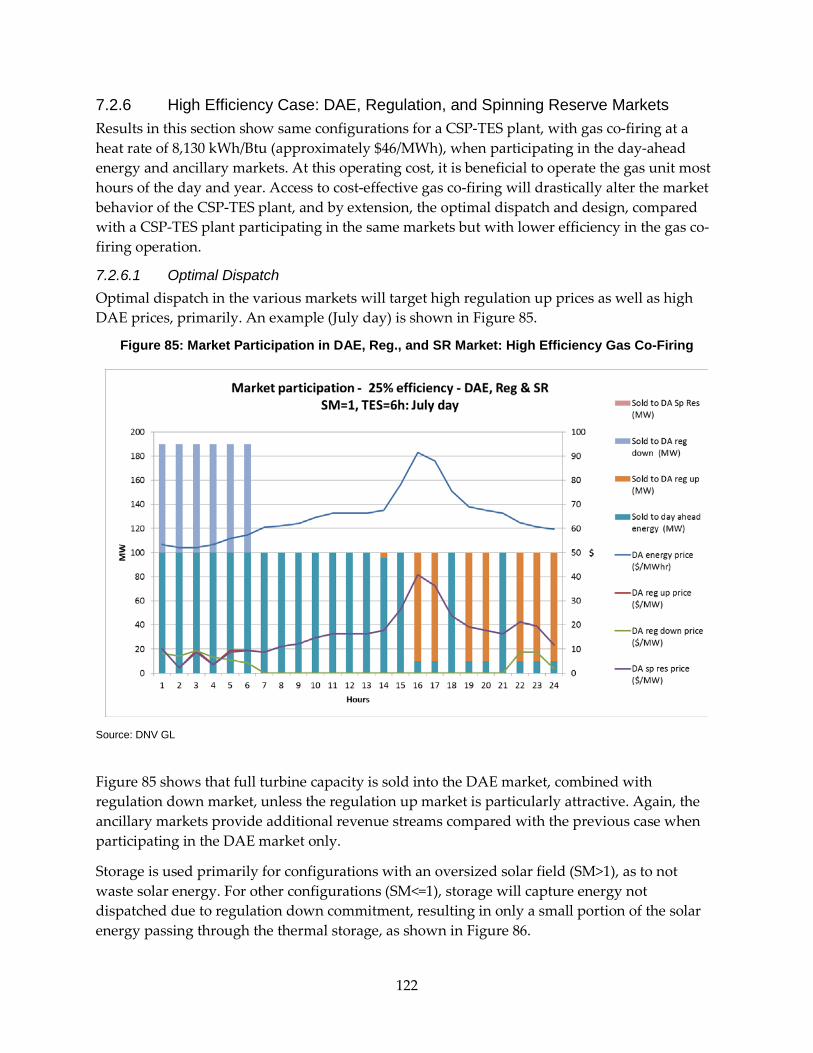
7.2.6 High Efficiency Case: DAE, Regulation, and Spinning Reserve Markets Results in this section show same configurations for a CSP-TES plant, with gas co-firing at a heat rate of 8,130 kWh/Btu (approximately $46/MWh), when participating in the day-ahead energy and ancillary markets. At this operating cost, it is beneficial to operate the gas unit most hours of the day and year. Access to cost-effective gas co-firing will drastically alter the market behavior of the CSP-TES plant, and by extension, the optimal dispatch and design, compared with a CSP-TES plant participating in the same markets but with lower efficiency in the gas co-firing operation.
7.2.6.1 Optimal Dispatch Optimal dispatch in the various markets will target high regulation up prices as well as high DAE prices, primarily. An example (July day) is shown in Figure 85.
Figure 85: Market Participation in DAE, Reg., and SR Market: High Efficiency Gas Co-Firing
Source: DNV GL
Figure 85 shows that full turbine capacity is sold into the DAE market, combined with regulation down market, unless the regulation up market is particularly attractive. Again, the ancillary markets provide additional revenue streams compared with the previous case when participating in the DAE market only.
Storage is used primarily for configurations with an oversized solar field (SM>1), as to not waste solar energy. For other configurations (SM<=1), storage will capture energy not dispatched due to regulation down commitment, resulting in only a small portion of the solar energy passing through the thermal storage, as shown in Figure 86.
122
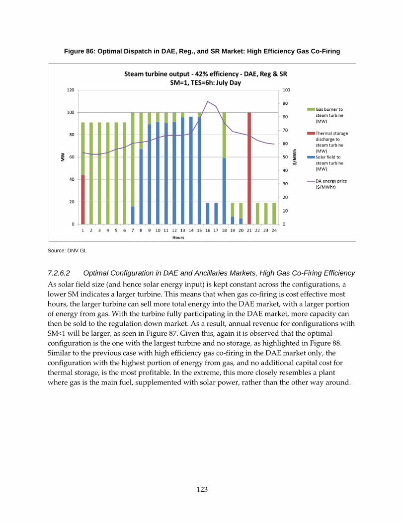
Figure 86: Optimal Dispatch in DAE, Reg., and SR Market: High Efficiency Gas Co-Firing
Source: DNV GL
7.2.6.2 Optimal Configuration in DAE and Ancillaries Markets, High Gas Co-Firing Efficiency As solar field size (and hence solar energy input) is kept constant across the configurations, a lower SM indicates a larger turbine. This means that when gas co-firing is cost effective most hours, the larger turbine can sell more total energy into the DAE market, with a larger portion of energy from gas. With the turbine fully participating in the DAE market, more capacity can then be sold to the regulation down market. As a result, annual revenue for configurations with SM<1 will be larger, as seen in Figure 87. Given this, again it is observed that the optimal configuration is the one with the largest turbine and no storage, as highlighted in Figure 88. Similar to the previous case with high efficiency gas co-firing in the DAE market only, the configuration with the highest portion of energy from gas, and no additional capital cost for thermal storage, is the most profitable. In the extreme, this more closely resembles a plant where gas is the main fuel, supplemented with solar power, rather than the other way around.
123
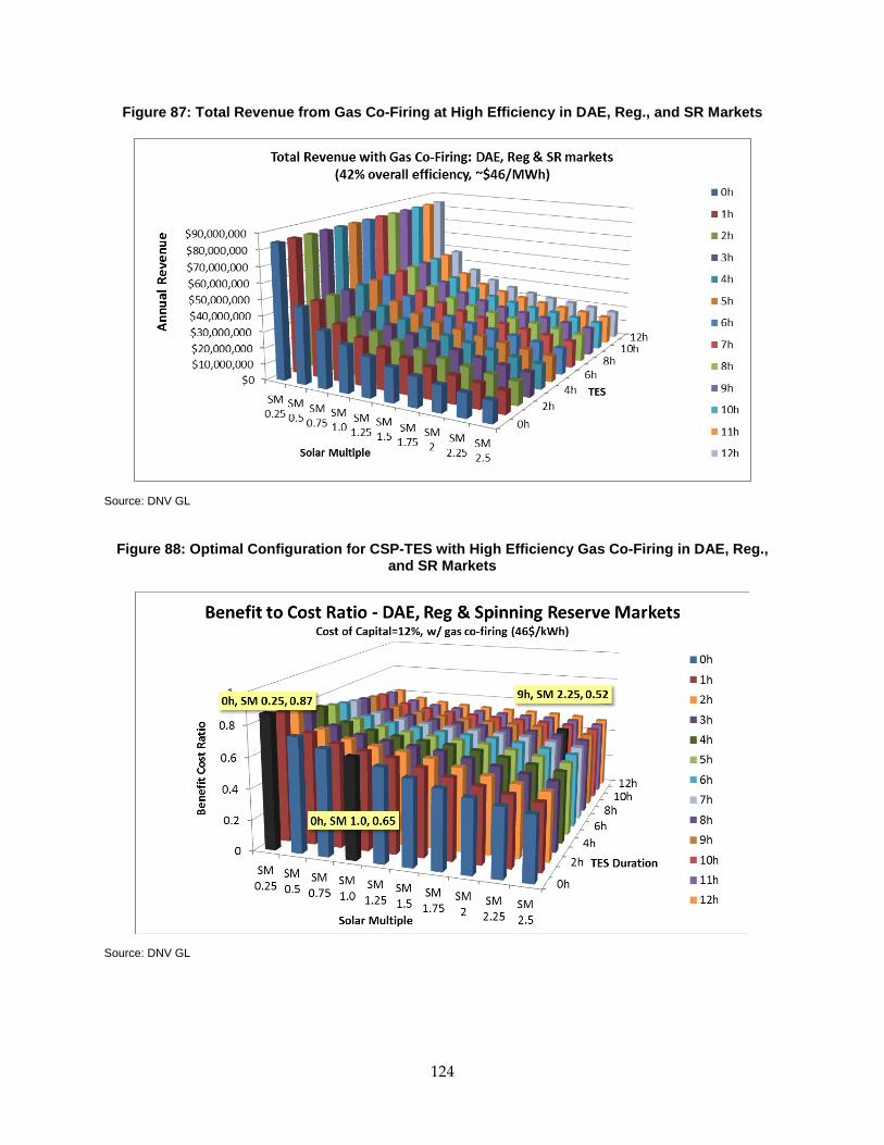
Figure 87: Total Revenue from Gas Co-Firing at High Efficiency in DAE, Reg., and SR Markets
Source: DNV GL
Figure 88: Optimal Configuration for CSP-TES with High Efficiency Gas Co-Firing in DAE, Reg., and SR Markets
Source: DNV GL
124
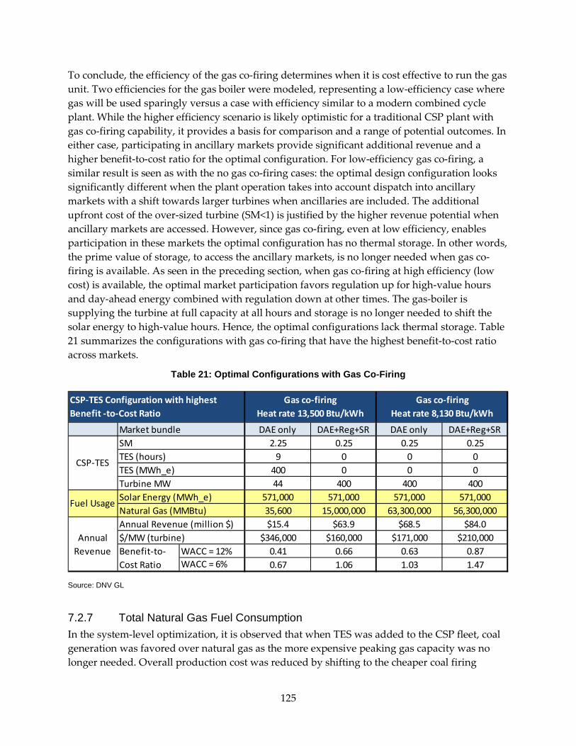
To conclude, the efficiency of the gas co-firing determines when it is cost effective to run the gas unit. Two efficiencies for the gas boiler were modeled, representing a low-efficiency case where gas will be used sparingly versus a case with efficiency similar to a modern combined cycle plant. While the higher efficiency scenario is likely optimistic for a traditional CSP plant with gas co-firing capability, it provides a basis for comparison and a range of potential outcomes. In either case, participating in ancillary markets provide significant additional revenue and a higher benefit-to-cost ratio for the optimal configuration. For low-efficiency gas co-firing, a similar result is seen as with the no gas co-firing cases: the optimal design configuration looks significantly different when the plant operation takes into account dispatch into ancillary markets with a shift towards larger turbines when ancillaries are included. The additional upfront cost of the over-sized turbine (SM<1) is justified by the higher revenue potential when ancillary markets are accessed. However, since gas co-firing, even at low efficiency, enables participation in these markets the optimal configuration has no thermal storage. In other words, the prime value of storage, to access the ancillary markets, is no longer needed when gas co-firing is available. As seen in the preceding section, when gas co-firing at high efficiency (low cost) is available, the optimal market participation favors regulation up for high-value hours and day-ahead energy combined with regulation down at other times. The gas-boiler is supplying the turbine at full capacity at all hours and storage is no longer needed to shift the solar energy to high-value hours. Hence, the optimal configurations lack thermal storage. Table 21 summarizes the configurations with gas co-firing that have the highest benefit-to-cost ratio across markets.
Table 21: Optimal Configurations with Gas Co-Firing
Source: DNV GL
7.2.7 Total Natural Gas Fuel Consumption In the system-level optimization, it is observed that when TES was added to the CSP fleet, coal generation was favored over natural gas as the more expensive peaking gas capacity was no longer needed. Overall production cost was reduced by shifting to the cheaper coal firing
Market bundle DAE only DAE+Reg+SR DAE only DAE+Reg+SR2.25 0.25 0.25 0.25
9 0 0 0400 0 0 044 400 400 400
571,000 571,000 571,000 571,00035,600 15,000,000 63,300,000 56,300,000$15.4 $63.9 $68.5 $84.0
$346,000 $160,000 $171,000 $210,000WACC = 12% 0.41 0.66 0.63 0.87WACC = 6% 0.67 1.06 1.03 1.47
Fuel Usage Solar Energy (MWh_e)Natural Gas (MMBtu)
Annual Revenue
Annual Revenue (million $)$/MW (turbine)Benefit-to-Cost Ratio
CSP-TES Configuration with highest Benefit -to-Cost Ratio
Gas co-firing Heat rate 13,500 Btu/kWh
Gas co-firing Heat rate 8,130 Btu/kWh
CSP-TES
SMTES (hours)TES (MWh_e)Turbine MW
125
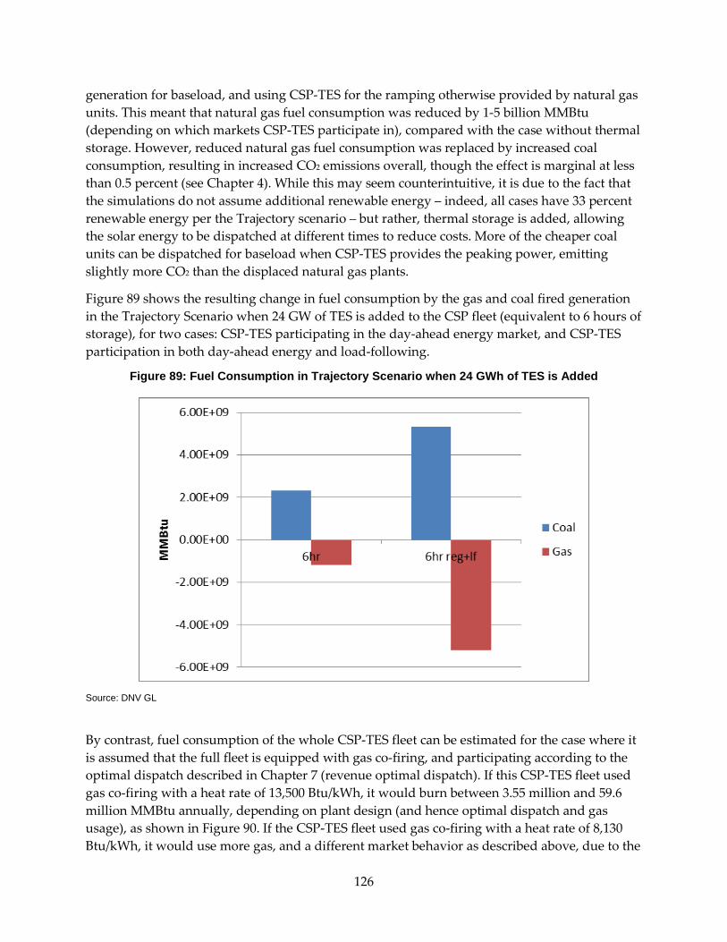
generation for baseload, and using CSP-TES for the ramping otherwise provided by natural gas units. This meant that natural gas fuel consumption was reduced by 1-5 billion MMBtu (depending on which markets CSP-TES participate in), compared with the case without thermal storage. However, reduced natural gas fuel consumption was replaced by increased coal consumption, resulting in increased CO2 emissions overall, though the effect is marginal at less than 0.5 percent (see Chapter 4). While this may seem counterintuitive, it is due to the fact that the simulations do not assume additional renewable energy – indeed, all cases have 33 percent renewable energy per the Trajectory scenario – but rather, thermal storage is added, allowing the solar energy to be dispatched at different times to reduce costs. More of the cheaper coal units can be dispatched for baseload when CSP-TES provides the peaking power, emitting slightly more CO2 than the displaced natural gas plants.
Figure 89 shows the resulting change in fuel consumption by the gas and coal fired generation in the Trajectory Scenario when 24 GW of TES is added to the CSP fleet (equivalent to 6 hours of storage), for two cases: CSP-TES participating in the day-ahead energy market, and CSP-TES participation in both day-ahead energy and load-following.
Figure 89: Fuel Consumption in Trajectory Scenario when 24 GWh of TES is Added
Source: DNV GL
By contrast, fuel consumption of the whole CSP-TES fleet can be estimated for the case where it is assumed that the full fleet is equipped with gas co-firing, and participating according to the optimal dispatch described in Chapter 7 (revenue optimal dispatch). If this CSP-TES fleet used gas co-firing with a heat rate of 13,500 Btu/kWh, it would burn between 3.55 million and 59.6 million MMBtu annually, depending on plant design (and hence optimal dispatch and gas usage), as shown in Figure 90. If the CSP-TES fleet used gas co-firing with a heat rate of 8,130 Btu/kWh, it would use more gas, and a different market behavior as described above, due to the
126
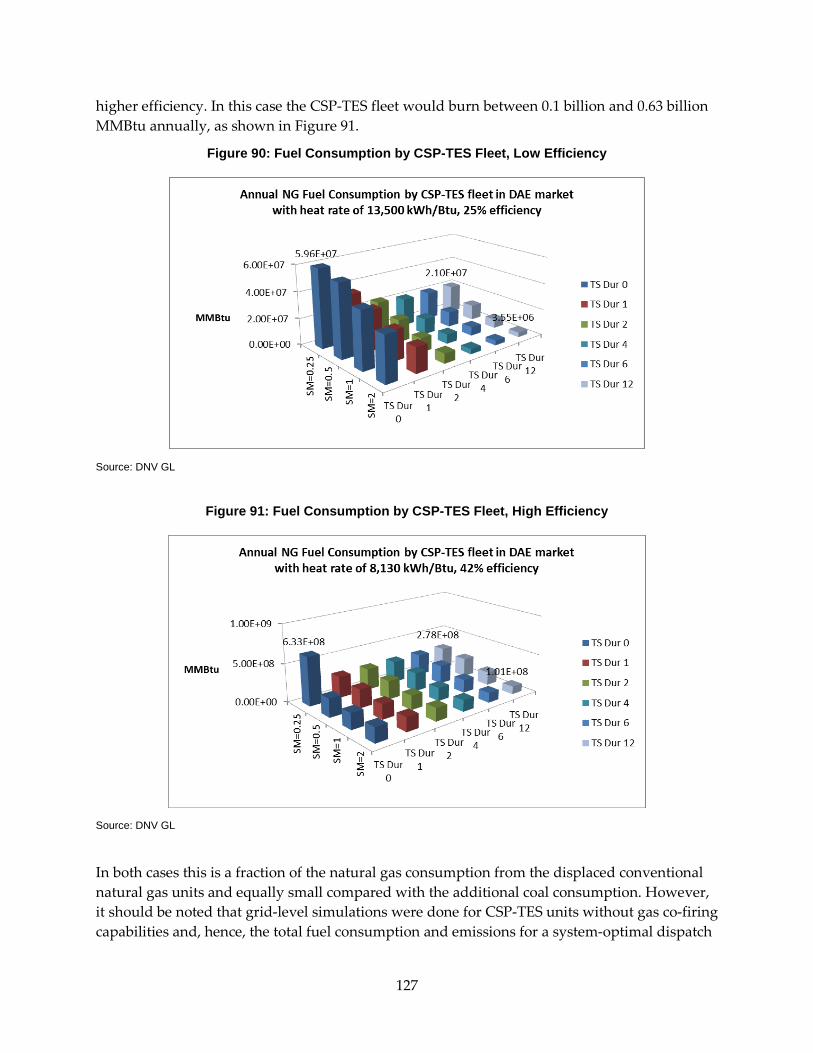
higher efficiency. In this case the CSP-TES fleet would burn between 0.1 billion and 0.63 billion MMBtu annually, as shown in Figure 91.
Figure 90: Fuel Consumption by CSP-TES Fleet, Low Efficiency
Source: DNV GL
Figure 91: Fuel Consumption by CSP-TES Fleet, High Efficiency
Source: DNV GL
In both cases this is a fraction of the natural gas consumption from the displaced conventional natural gas units and equally small compared with the additional coal consumption. However, it should be noted that grid-level simulations were done for CSP-TES units without gas co-firing capabilities and, hence, the total fuel consumption and emissions for a system-optimal dispatch
127
of a CSP-TES fleet with gas co-firing is not directly known. In other words, in order to determine the trade-off between coal and natural gas consumption and resulting total emissions at a system level when the CSP-TES fleet is equipped with gas co-firing capabilities, a system-level simulation with CSP-TES plants using natural gas would need to be performed. This is outside the scope of the current study.
7.3 Summary of Results from Plant-Level Analysis The economic performance for CSP systems is evaluated over variations in the solar multiple and duration of the storage device. Solar Multiple (SM) is a ratio indicating the size of the solar field relative to the size of the turbine generator. The size of the solar field is held constant, in order to have the same energy input to all plant confugurations, while the size of the turbine is varied in order to change the Solar Multiple (SM). In other words, SM less than one (SM < 1) means an over-sized turbine relative to the solar field and vice versa. It is also assumed that the solar field is the largest capital expense for the project. For any system configuration, an 8760-hour operational simulation is carried out to evaluate the cash-flows of the CSP-TES system over one year. The market participation model optimizes potential revenue through participation in day-ahead wholesale market services such as energy, regulation and spinning reserve markets. The optimization is carried out for one day at a time with 1-hour granularity. The operational optimization indicates the most profitable revenue streams and market services for each CSP-TES configuration. Given capital costs and other annual costs, different configurations can be compared through a benefit-to-cost analysis. It should be noted that the benefit-to-cost ratio should not be regarded in absolute terms, rather, it should be seen as a metric that provides uniform basis for comparison of different configurations. While our operations model is accurate under given wholesale prices, the cost assessment is based on assumptions and inputs from publicly available data, and feed-back from the Project Advisory Committee. In reality, while CSP-TES plants operating in CAISO would be exposed to similar wholesale market scenarios, each individual project would face different investment and cost conditions. The cost-benefit analysis tends to demonstrate the trade-off between gaining more revenue and the increase in upfront and operational costs.
The detailed thermodynamic models of selected technologies, namely, tower and trough collectors, two-tank direct, and EPCM thermal storage are developed and the results of the system-level analysis are verified against these simulations. The market participation model is run for various configurations including solar multiples of 0.25-2.5 coupled with 0-12 hours of storage, with and without an additional gas co-firing system. Gas co-firing is tested for two efficiencies of the gas burner. Both energy and ancillary service market prices are obtained from the CAISO production cost model in PLEXOS, which was used for the system level analysis.
7.3.1 Optimizing CSP-TES Plant Design without Gas Co-Firing In the absence of gas co-firing, thermal energy storage provides significant additional value to the plant operator. In particular, thermal storage enables participation in Ancillary Markets, providing significant additional revenue.
128
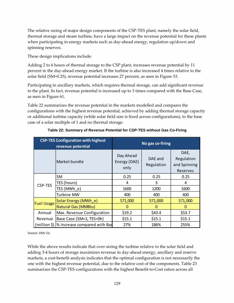
The relative sizing of major design components of the CSP-TES plant, namely the solar field, thermal storage and steam turbine, have a large impact on the revenue potential for these plants when participating in energy markets such as day-ahead energy, regulation up/down and spinning reserves.
These design implications include:
Adding 2 to 6 hours of thermal storage to the CSP plant, increases revenue potential by 11 percent in the day-ahead energy market. If the turbine is also increased 4 times relative to the solar field (SM=0.25), revenue potential increases 27 percent, as seen in Figure 53.
Participating in ancillary markets, which requires thermal storage, can add significant revenue to the plant. In fact, revenue potential is increased up to 3 times compared with the Base Case, as seen in Figure 61.
Table 22 summarizes the revenue potential in the markets modelled and compares the configurations with the highest revenue potential, achieved by adding thermal storage capacity or additional turbine capacity (while solar field size is fixed across configurations), to the base case of a solar multiple of 1 and no thermal storage.
Table 22: Summary of Revenue Potential for CSP-TES without Gas Co-Firing
Source: DNV GL
While the above results indicate that over-sizing the turbine relative to the solar field and adding 3-4 hours of storage maximizes revenue in day-ahead energy, ancillary and reserve markets, a cost-benefit analysis indicates that the optimal configuration is not necessarily the one with the highest revenue potential, due to the relative cost of the components. Table 23 summarizes the CSP-TES configurations with the highest Benefit-to-Cost ratios across all
Market bundleDay Ahead
Energy (DAE) only
DAE and Regulation
DAE, Regulation
and Spinning Reserves
0.25 0.25 0.254 3 4
1600 1200 1600400 400 400
571,000 571,000 571,0000 0 0
$19.2 $43.4 $53.7Base Case (SM=1, TES=0h) $15.1 $15.1 $15.1% Increase compared with Bas 27% 186% 255%
CSP-TES Configuration with highest revenue potential
No gas co-firing
CSP-TES
SMTES (hours)TES (MWh_e)Turbine MW
Fuel Usage Solar Energy (MWh_e)Natural Gas (MMBtu)
Annual Revenue
(million $)
Max. Revenue Configuration
129
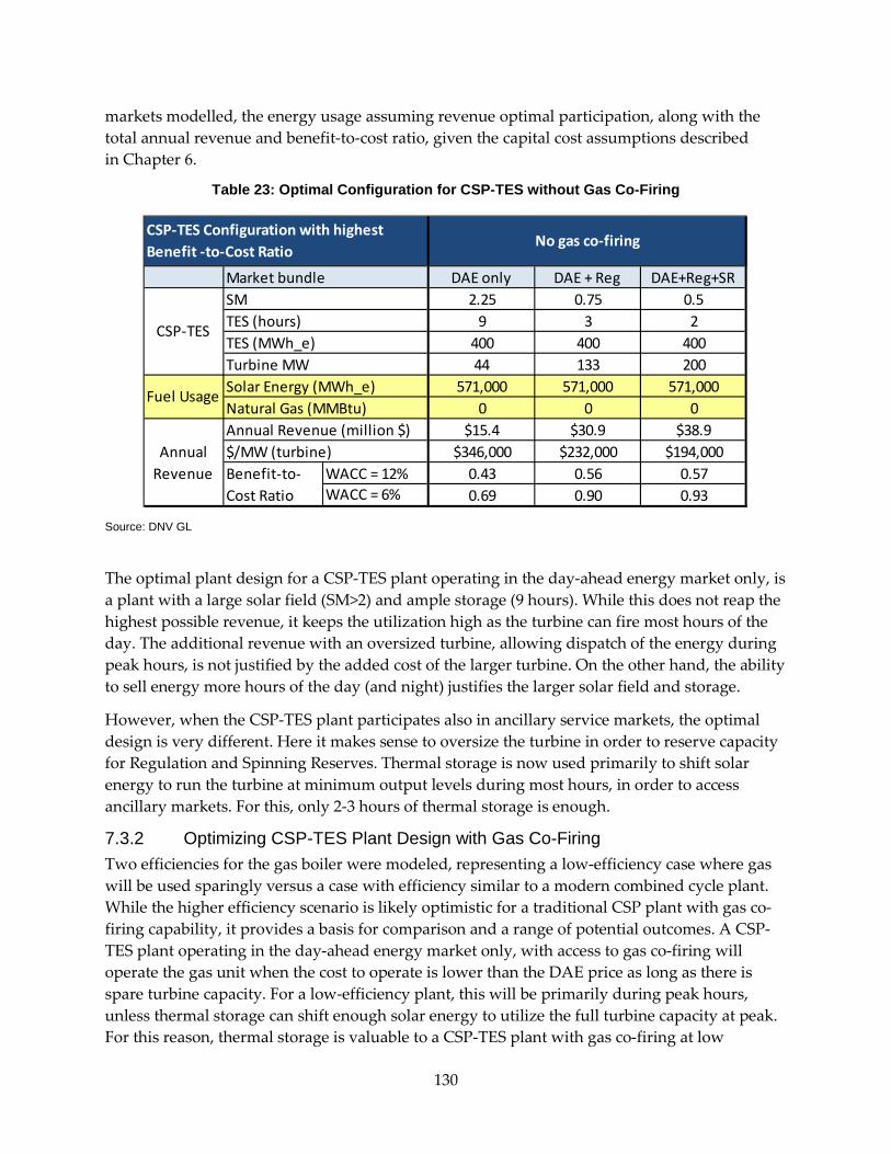
markets modelled, the energy usage assuming revenue optimal participation, along with the total annual revenue and benefit-to-cost ratio, given the capital cost assumptions described in Chapter 6.
Table 23: Optimal Configuration for CSP-TES without Gas Co-Firing
Source: DNV GL
The optimal plant design for a CSP-TES plant operating in the day-ahead energy market only, is a plant with a large solar field (SM>2) and ample storage (9 hours). While this does not reap the highest possible revenue, it keeps the utilization high as the turbine can fire most hours of the day. The additional revenue with an oversized turbine, allowing dispatch of the energy during peak hours, is not justified by the added cost of the larger turbine. On the other hand, the ability to sell energy more hours of the day (and night) justifies the larger solar field and storage.
However, when the CSP-TES plant participates also in ancillary service markets, the optimal design is very different. Here it makes sense to oversize the turbine in order to reserve capacity for Regulation and Spinning Reserves. Thermal storage is now used primarily to shift solar energy to run the turbine at minimum output levels during most hours, in order to access ancillary markets. For this, only 2-3 hours of thermal storage is enough.
7.3.2 Optimizing CSP-TES Plant Design with Gas Co-Firing Two efficiencies for the gas boiler were modeled, representing a low-efficiency case where gas will be used sparingly versus a case with efficiency similar to a modern combined cycle plant. While the higher efficiency scenario is likely optimistic for a traditional CSP plant with gas co-firing capability, it provides a basis for comparison and a range of potential outcomes. A CSP-TES plant operating in the day-ahead energy market only, with access to gas co-firing will operate the gas unit when the cost to operate is lower than the DAE price as long as there is spare turbine capacity. For a low-efficiency plant, this will be primarily during peak hours, unless thermal storage can shift enough solar energy to utilize the full turbine capacity at peak. For this reason, thermal storage is valuable to a CSP-TES plant with gas co-firing at low
Market bundle DAE only DAE + Reg DAE+Reg+SR2.25 0.75 0.5
9 3 2400 400 40044 133 200
571,000 571,000 571,0000 0 0
$15.4 $30.9 $38.9$346,000 $232,000 $194,000
WACC = 12% 0.43 0.56 0.57WACC = 6% 0.69 0.90 0.93
CSP-TES Configuration with highest Benefit -to-Cost Ratio
No gas co-firing
CSP-TES
SMTES (hours)TES (MWh_e)Turbine MW
Fuel Usage Solar Energy (MWh_e)Natural Gas (MMBtu)
Annual Revenue
Annual Revenue (million $)$/MW (turbine)Benefit-to-Cost Ratio
130
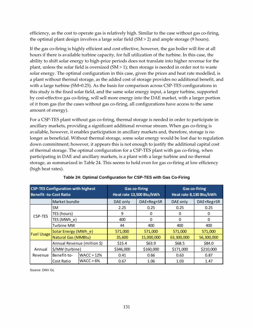
efficiency, as the cost to operate gas is relatively high. Similar to the case without gas co-firing, the optimal plant design involves a large solar field (SM > 2) and ample storage (9 hours).
If the gas co-firing is highly efficient and cost effective, however, the gas boiler will fire at all hours if there is available turbine capacity, for full utilization of the turbine. In this case, the ability to shift solar energy to high-price periods does not translate into higher revenue for the plant, unless the solar field is oversized (SM > 1); then storage is needed in order not to waste solar energy. The optimal configuration in this case, given the prices and heat rate modelled, is a plant without thermal storage, as the added cost of storage provides no additional benefit, and with a large turbine (SM=0.25). As the basis for comparison across CSP-TES configurations in this study is the fixed solar field, and the same solar energy input, a larger turbine, supported by cost-effective gas co-firing, will sell more energy into the DAE market, with a larger portion of it from gas (for the cases without gas co-firing, all configurations have access to the same amount of energy).
For a CSP-TES plant without gas co-firing, thermal storage is needed in order to participate in ancillary markets, providing a significant additional revenue stream. When gas co-firing is available, however, it enables participation in ancillary markets and, therefore, storage is no longer as beneficial. Without thermal storage, some solar energy would be lost due to regulation down commitment; however, it appears this is not enough to justify the additional capital cost of thermal storage. The optimal configuration for a CSP-TES plant with gas co-firing, when participating in DAE and ancillary markets, is a plant with a large turbine and no thermal storage, as summarized in Table 24. This seems to hold even for gas co-firing at low efficiency (high heat rates).
Table 24: Optimal Configuration for CSP-TES with Gas Co-Firing
Source: DNV GL
Market bundle DAE only DAE+Reg+SR DAE only DAE+Reg+SR2.25 0.25 0.25 0.25
9 0 0 0400 0 0 044 400 400 400
571,000 571,000 571,000 571,00035,600 15,000,000 63,300,000 56,300,000$15.4 $63.9 $68.5 $84.0
$346,000 $160,000 $171,000 $210,000WACC = 12% 0.41 0.66 0.63 0.87WACC = 6% 0.67 1.06 1.03 1.47
Fuel Usage Solar Energy (MWh_e)Natural Gas (MMBtu)
Annual Revenue
Annual Revenue (million $)$/MW (turbine)Benefit-to-Cost Ratio
CSP-TES Configuration with highest Benefit -to-Cost Ratio
Gas co-firing Heat rate 13,500 Btu/kWh
Gas co-firing Heat rate 8,130 Btu/kWh
CSP-TES
SMTES (hours)TES (MWh_e)Turbine MW
131
CHAPTER 8: Conclusions The study shows that significant benefits can be accrued, both to the California grid and energy markets in terms of production cost savings and improved grid performance, and to the plant operator in terms of revenue, when concentrating solar power plants participate in day-ahead ancillary markets in addition to delivering energy. For the plant to be able to participate in these markets, however, it needs to be dispatchable. This can be achieved either by coupling the plant with thermal energy storage or with natural gas co-firing capabilities.
From the grid and market system perspective, having additional ramping and regulation capacity in the context of increasing renewables and less system flexibility is attractive. The study shows that concentrating solar power plants coupled with thermal energy storage can provide this capability using renewable energy, and hence help meet future RPS goals, while providing additional economic benefit to the plant owner.
For the plant owner, the additional revenue appears to economically justify adding thermal energy storage or gas co-firing capability to the CSP plant in order to access these ancillary markets. However, the revenue potential and benefit of capital investments is highly dependent on system design and operational strategy. In other words, the sizing of major plant components should reflect the future market participation strategy. It appears that a plant designed for participation in regulation and spinning reserve markets would reap higher revenue and benefit if designed with a relatively larger turbine and only 2-3 hours of energy storage, while a plant intended for energy delivery only should be designed with a relatively large solar field and 8-9 hours of energy storage. When gas co-firing capabilities are added, the value of TES is generally decreased as the flexibility needed to participate in ancillary markets – ramping and dispatchability - can be achieved also with the gas boiler. The efficiency of the gas boiler will impact the economics of operating the gas unit and, by extension, the optimal sizing and market participation strategy as well.
Overall, benefits are maximized for both the grid system and the plant owner when the CSP-TES plant is designed for flexibility, particularly if the CSP-TES plant can participate in the regulation market. Flexibility for a 100% renewable plant can be achieved by adding thermal storage and 2-3 hours of storage appears adequate for this. Another alternative is to add gas co-firing capability, especially if the plant can operate at a high overall efficiency.
8.1 Summary of Results 8.1.1 System-Level Analysis of California Grid and Market Operations A number of benefits at the system-level can be realized when CSP is coupled with TES (CSP-TES) as CSP-TES can improve both economics and system performance. In general, production costs can be lowered by leveraging the dispatchability and flexibility of the CSP-TES units. By allowing the CSP-TES to follow a day-ahead energy schedule, lower overall production cost from energy time-shifting to high-value hours can be accomplished, along with less import during evening peak hours. However, CSP-TES cannot capture lowest-cost energy overnight as
132
the TES can only charge during daylight hours, hence this benefit is modest.As a result, savings of up to $19 million may be realizable in California when the CSP-TES fleet (3.2 gigawatts) provides peaking energy.
Significant energy production cost savings for the system overall could be realized if CSP-TES provides regulation and load-following, with savings tied to the total capacity of CSP that can be set aside for regulation, as compared with CSP without TES and without the ability to provide regulation and load-following. If load-following is provided, in addition to day-ahead energy, savings may increase to around $44 million. Further, if a large portion of the CSP capacity can provide regulation savings of up to $64 million are possible. Note that this study does not quantify the cost of procuring regulation, but rather, the savings in energy production when CSP-TES is available to provide regulation or load-following. How CSP will affect regulation prices as bid by conventional units and cleared in the market is more complex; at some point if the penetration of CSP increases, it will cease to be a price taker at all hours and CSP facilities would have to determine how to price regulation offers. Generally speaking, regulation prices are quite low unless there are associated energy sales opportunity costs at peak or minimum energy delivery costs at off peak to consider.
In addition, reduced variability on the system results in lower overall ACE, which translates to reduced system regulation and load-following requirements. This reduced need for regulation is a significant system cost saving. If, for instance, regulation capacity can be reduced by 50% savings of up to $130 million may accrue to California (see Section 0 for reference), in addition to the savings from the services provided from the CSP-TES fleet. Lastly, coupling TES with the CSP fleet provides an emissions-neutral hedge against forecast error in the renewable energy production of CSP. From a system performance perspective, two hours of TES is as effective as six hours of storage in providing system flexibility and improving performance metrics, such as ACE, CPS1, and CPS2. In addition, two hours of storage provide similar benefits as six hours of storage in reducing overall production cost, when the CSP-TES capacity is available for regulation and load-following. Note that spinning reserves have not been evaluated as part of the system-level economic optimization, but is addressed at the plant level revenue optimization. Further discussion of these results can be found in Chapter 4.
8.1.2 Plant Dynamics and Performance Detailed thermodynamic modelling suggests that existing CSP technologies, such as solar tower, trough and Fresnel reflector, coupled with existing and emerging TES technologies evaluated in this study, such as two-tank molten salt and single tank technologies with phase change materials, can be operated in a way that allows participation in ancillary markets. In other words, they have the flexibility and ramping capacity, if operated correctly, to follow a regulation signal.
While there is some difference in performance between CSP technologies Tower and Trough, these can be addressed at the design stage (storage sizing) or operationally, by adjusting over-night storage levels to account for the time it takes to heat the heat-transfer fluids in the early morning.
133
8.1.3 Plant-Level Revenue and Design Optimization Overall, the results show that participation in both day-ahead energy and ancillary markets provide higher revenue, as well a better return on investment, than participation in the day-ahead energy market only. In addition, the optimal plant configuration is highly dependent on the market participation scheme:
In the Day-Ahead Energy market a large solar field and correspondingly large thermal storage is beneficial, for plants without gas co-firing or with gas co-firing at low efficiency. The optimal configuration in this case is a plant with 9 hours of storage and a solar multiple of 2.25.
When participating in ancillary markets, a larger turbine is beneficial in order to reserve more capacity. In this case, shorter duration storage, or gas co-firing, is enough to support this participation. The optimal configuration for a plant without gas co-firing is with 2-3 hours of storage and a solar multiple of 0.5 to 0.75. The optimal configuration for a plant with gas co-firing is simply a plant with no storage and lots of turbine capacity (solar multiple of 0.25 was the largest modeled in this study).
It is noted that while the benefits of thermal storage are somewhat diminished in the presence of gas co-firing (depending upon the gas price and boiler efficiency used), this analysis does not take into account the impact of forecast error in either gas prices or solar irradiation, and the presence of both thermal storage and gas co-firing may provide a hedge against these uncertainties. Further analysis and modeling is needed to reveal the value of thermal storage as a hedge against these uncertainties. It should also be noted that a CSP-TES plant with gas co-firing capabilities may not be eligible to count towards RSP goals or other renewables incentives or may have restrictions on the mount of gas it is allowed to use. The results from the plant-level revenue and design optimization are discussed in further detail in Chapter 7.
134
CHAPTER 9: Technology Transfer Activities The following activities are completed in order to bring the outcomes of the project to the market:
• Summary article in IEEE paper on the outcomes of the grid and market level analysis of the study
• Article on the DNV GL Utility of the Future blog on the results from the plant-level analysis of the study
• A podium presentation and panel discussion at the Solar Power International 2014 conference in Las Vegas on October 22, 2014.
• A workshop at the CEC on May 1st 2015, where DNV GL presented the results of the Final Report as well as overall conclusions.
135
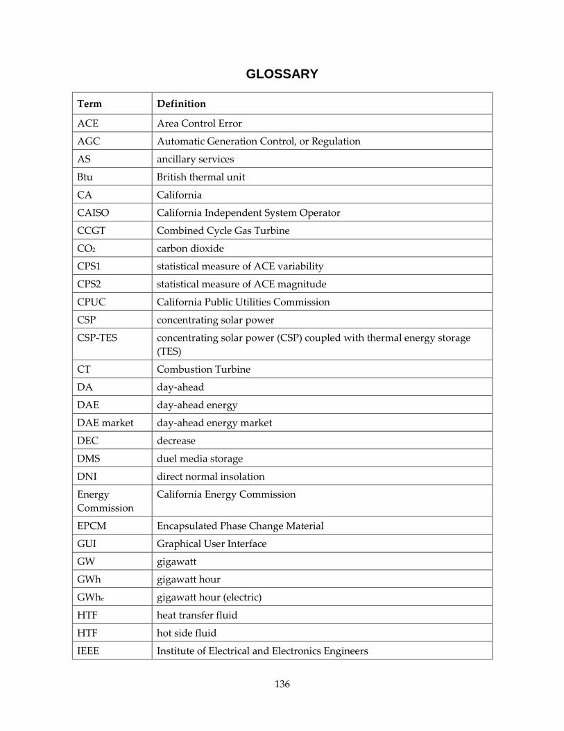
GLOSSARY
Term Definition
ACE Area Control Error
AGC Automatic Generation Control, or Regulation
AS ancillary services
Btu British thermal unit
CA California
CAISO California Independent System Operator
CCGT Combined Cycle Gas Turbine
CO2 carbon dioxide
CPS1 statistical measure of ACE variability
CPS2 statistical measure of ACE magnitude
CPUC California Public Utilities Commission
CSP concentrating solar power
CSP-TES concentrating solar power (CSP) coupled with thermal energy storage (TES)
CT Combustion Turbine
DA day-ahead
DAE day-ahead energy
DAE market day-ahead energy market
DEC decrease
DMS duel media storage
DNI direct normal insolation
Energy Commission
California Energy Commission
EPCM Encapsulated Phase Change Material
GUI Graphical User Interface
GW gigawatt
GWh gigawatt hour
GWhe gigawatt hour (electric)
HTF heat transfer fluid
HTF hot side fluid
IEEE Institute of Electrical and Electronics Engineers
136
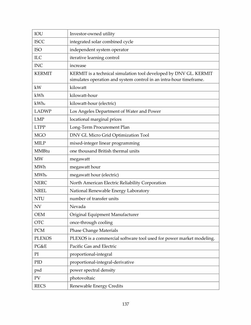
IOU Investor-owned utility
ISCC integrated solar combined cycle
ISO independent system operator
ILC iterative learning control
INC increase
KERMIT KERMIT is a technical simulation tool developed by DNV GL. KERMIT simulates operation and system control in an intra-hour timeframe.
kW kilowatt
kWh kilowatt-hour
kWhe kilowatt-hour (electric)
LADWP Los Angeles Department of Water and Power
LMP locational marginal prices
LTPP Long-Term Procurement Plan
MGO DNV GL Micro Grid Optimization Tool
MILP mixed-integer linear programming
MMBtu one thousand British thermal units
MW megawatt
MWh megawatt hour
MWhe megawatt hour (electric)
NERC North American Electric Reliability Corporation
NREL National Renewable Energy Laboratory
NTU number of transfer units
NV Nevada
OEM Original Equipment Manufacturer
OTC once-through cooling
PCM Phase Change Materials
PLEXOS PLEXOS is a commercial software tool used for power market modeling.
PG&E Pacific Gas and Electric
PI proportional-integral
PID proportional-integral-derivative
psd power spectral density
PV photovoltaic
RECS Renewable Energy Credits
137
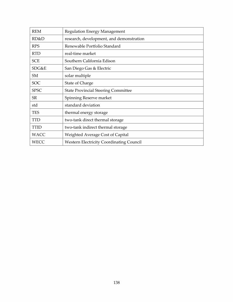
REM Regulation Energy Management
RD&D research, development, and demonstration
RPS Renewable Portfolio Standard
RTD real-time market
SCE Southern California Edison
SDG&E San Diego Gas & Electric
SM solar multiple
SOC State of Charge
SPSC State Provincial Steering Committee
SR Spinning Reserve market
std standard deviation
TES thermal energy storage
TTD two-tank direct thermal storage
TTID two-tank indirect thermal storage
WACC Weighted Average Cost of Capital
WECC Western Electricity Coordinating Council
138
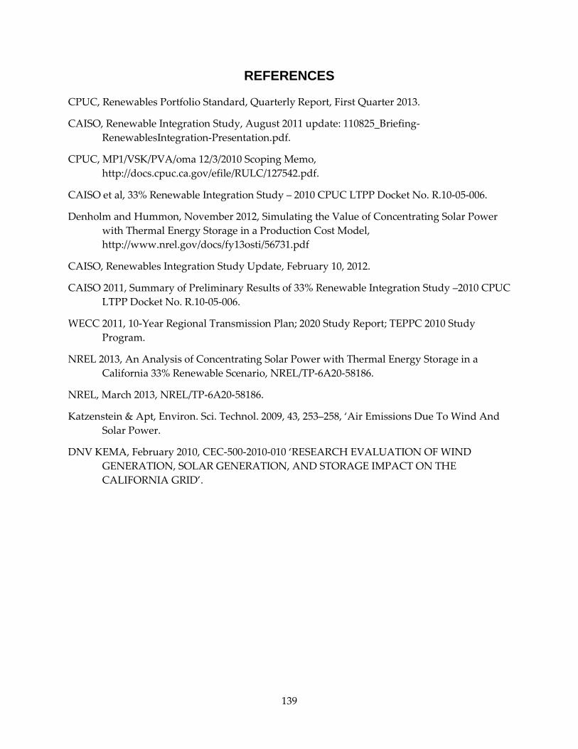
REFERENCES
CPUC, Renewables Portfolio Standard, Quarterly Report, First Quarter 2013.
CAISO, Renewable Integration Study, August 2011 update: 110825_Briefing-RenewablesIntegration-Presentation.pdf.
CPUC, MP1/VSK/PVA/oma 12/3/2010 Scoping Memo, http://docs.cpuc.ca.gov/efile/RULC/127542.pdf.
CAISO et al, 33% Renewable Integration Study – 2010 CPUC LTPP Docket No. R.10-05-006.
Denholm and Hummon, November 2012, Simulating the Value of Concentrating Solar Power with Thermal Energy Storage in a Production Cost Model, http://www.nrel.gov/docs/fy13osti/56731.pdf
CAISO, Renewables Integration Study Update, February 10, 2012.
CAISO 2011, Summary of Preliminary Results of 33% Renewable Integration Study –2010 CPUC LTPP Docket No. R.10-05-006.
WECC 2011, 10-Year Regional Transmission Plan; 2020 Study Report; TEPPC 2010 Study Program.
NREL 2013, An Analysis of Concentrating Solar Power with Thermal Energy Storage in a California 33% Renewable Scenario, NREL/TP-6A20-58186.
NREL, March 2013, NREL/TP-6A20-58186.
Katzenstein & Apt, Environ. Sci. Technol. 2009, 43, 253–258, ‘Air Emissions Due To Wind And Solar Power.
DNV KEMA, February 2010, CEC-500-2010-010 ‘RESEARCH EVALUATION OF WIND GENERATION, SOLAR GENERATION, AND STORAGE IMPACT ON THE CALIFORNIA GRID’.
139
APPENDICES Appendix A: KERMIT Model
Appendix B: Production Cost Modeling
Appendix C: Renewable Generation Modeling
Appendix D: Thermodynamic Plant Models
Appendix E: Detailed Results from Thermodynamic Plant Model Simulations
Appendix F: MGO – Operational Optimization Model
Appendix G: Input Data for MGO 2020 Simulations
These appendices are available as a separate volume, publication number CEC-500-2015-078-AP.